Chap5: Markov Chain

Markov Property

A sequence of random variables {Xn} is called a Markov chain if it has the Markovproperty:

P{Xk = i|Xk−1 = j,Xk−2, · · · , X1} = P{Xk = i|Xk−1 = j}

States are usually labelled {(0, )1, 2, · · · }, and state space can be finite or infinite.

• First order Markov assumption (memoryless):

P (qt = i | qt−1 = j, qt−2 = k, · · · ) = P (qt = i | qt−1 = j)

• Stationarity:P (qt = i | qt−1 = j) = P (qt+l = i | qt+l−1 = j)

1

Homogeneity:

Chap5: Markov Chain

1-D Random Walk

• Time is slotted.

• The walker flips a coin every time slot to decide which way to go:

X(t + 1) =

⎧⎨⎩

X(t) + 1 w.p.p

X(t) − 1 w.p.(1 − p)

Figure 1: 1-D Random walk.

2

State No.

with probability pwith probability (1-p)

Chap5: Markov Chain

Homogeneous Markov chain

Definition: an homogeneous Markov Chain has Pn,n+1

ij = Pij for all n. The one-steptransition probabilities do not depend on time n.

Definition: the transition probability matrix is given by

P = [Pij ] =

⎡⎢⎢⎢⎢⎢⎢⎣

P00 P01 P02 · · ·P10 P11 P12 · · ·P20 P21 P22 · · ·

......

.... . .

⎤⎥⎥⎥⎥⎥⎥⎦

wherePij ≥ 0 and

∑j

Pij = 1

The n-step transition probability Pnij is the probability that a person in state i will be in state j

in n steps, that isPn

ij = Prob(Xn+m = j |Xm = i)

5

process

afterP

3

Chap5: Markov Chain

Illustrative example

The No-Claim Discount system in car insurance is a system where the premium chargeddepends on the policyholder’s claim record. This is usually modelled using a Markov chair.In an NCD scheme a policyholder’s premium will depend on whether or not they had a claim.

NCD level Discount %

0 0

1 25

2 50

If a policyholder has no claims in a year then they move to the next higher level of discount(unless they are already on the highest level, in which case they stay there). If a policyholderhas one or more claims in a year then they move to the next lower level of discount (unlessthey are already on the lowest level, in which case they stay there). The probability of noclaims in a year is assumed to be 0.9.

The state space of the Markov chain is 0,1,2 where state i corresponds to NCD level i.

64

Chap5: Markov Chain

The transition matrix is

P =

⎡⎢⎢⎣

0.1 0.9 0

0.1 0 0.9

0 0.1 0.9

⎤⎥⎥⎦

Example 1: (Forecasting the weather): suppose that the chance of rain tomorrow depends

on previous weather conditions only through whether or not it is raining today and not onpast weather conditions. Suppose also that if it rains today, then it will rain tomorrow withprobability α; and if it does not rain today, then it will rain tomorrow with probability β.

If we say that the process is in state 0 when it rains and state 1 when it does not rain, then theabove is a two-state markov chain whose transition probabilities are given by

P =

⎡⎣ α 1 − α

β 1 − β

⎤⎦

75

Chap5: Markov Chain

Classification of States

Some definition:

• A state i is said to be an absorbing state if Pii = 1 or, equivalently, Pij = 0 for anyj �= i.

• State j is accessible from state i if Pnij > 0 for some n ≥ 0. This is written as i → j, i

leads to j or j is accessible from i. Note that if i → j and j → k then i → k.

• State i and j communicate if i → j and j → i. This is written as i ↔ j. Note that i ↔ i

for all i, if i ↔ j then j ↔ i, and if i ↔ j and j ↔ k then i ↔ k.

• The class of states that communicate with state i is C(i) = {j ∈ S, i ↔ j}. Two statesthat communicate are in the same class. Note that for any two states i, j ∈ S eitherC(i) = C(j) or C(i) ∩ C(j) = Φ. Also if j ∈ C(i), then C(i) = C(j).

• A Markov chain is said to be irreducible if there is only one class. All states thereforecommunicate with each other.

11

s:

9

Chap5: Markov Chain

Example 3: Consider the Markov chain consisting of the three states 0,1,2 and having

transition probability matrix

P =

⎡⎢⎢⎣

12

12 0

12

14

14

0 13

23

⎤⎥⎥⎦

It is easy to verify that this Markov chain is irreducible. For example, it is possible to go fromstate 0 to state 2, since

0 → 1 → 2

That is, one way of getting from state 0 to state 2 is to go from state 0 to state 1 (withprobability 1/2) and then go from state 1 to state 2 (with probability 1/4).

12

It is also possible to go from state 2 to state 0, since 2 1 0

10

Chap5: Markov Chain

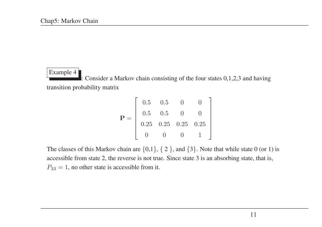
Example 4: Consider a Markov chain consisting of the four states 0,1,2,3 and having

transition probability matrix

P =

⎡⎢⎢⎢⎢⎢⎣

0.5 0.5 0 0

0.5 0.5 0 0

0.25 0.25 0.25 0.25

0 0 0 1

⎤⎥⎥⎥⎥⎥⎦

The classes of this Markov chain are {0,1}, { 2 }, and {3}. Note that while state 0 (or 1) isaccessible from state 2, the reverse is not true. Since state 3 is an absorbing state, that is,P33 = 1, no other state is accessible from it.

1311

Chap5: Markov Chain

Classification of States

Denote by fi the probability that the process starting in state i will at some future time returnto state i.

• State i is said to be recurrent if fi = 1. State i is said to be transient if fi < 1.

• If state i is recurrent then, starting in state i, the process will enter state i infinitely often.

• Starting in state i, if state i is transient, then the probability that the process will be instate i for exactly n ≥ 1 time periods is given by a Geometric distribution fn−1

i (1 − fi).The expected number of time periods that the process is in state i is 1/(1 − fi).

• A transient state will only be visited a finite number of times.

• In a finite state Markov chain, at least one state must be recurrent or that not all statescan be transient. For otherwise, after a finite number of times, no states will be visitedwhich is impossible.

• If state i is recurrent and state i communicates with state j(i ↔ j), then state j isrecurrent.

• If state i is transient and state i communicates with state j(i ↔ j), then state j istransient.

14

Definition: Recurrent and Transient StatesIn a Markov chain, a state i is transient if there exists a state j such that i j butj i; otherwise, if no such state j exists, then state i is recurrent.

Theorems:

12

Chap5: Markov Chain

• All states in a finite irreducible Markov chain are recurrent.

• A class of states is recurrent if all states in the class are Recurrent. A class of states istransient if all states in the class are transient

Example 5: consider a Markov chain with state space 0, 1, 2, 3, 4 and transition matrix

P =

⎡⎢⎢⎢⎢⎢⎢⎢⎢⎣

0.5 0.5 0 0 0

0.5 0.5 0 0 0

0 0 0.5 0.5 0

0 0 0.5 0.5 0

0.25 0.25 0 0 0.5

⎤⎥⎥⎥⎥⎥⎥⎥⎥⎦

Determine which states are recurrent and which states are transient.

1513

Chap5: Markov Chain

Example 6: consider a Markov chain with state space 0, 1, 2, 3, 4, 5 and transition matrix

P =

⎡⎢⎢⎢⎢⎢⎢⎢⎢⎢⎢⎢⎣

1 0 0 0 0 014

12

14 0 0 0

0 15

25

15 0 1

5

0 0 0 16

13

12

0 0 0 12 0 1

2

0 0 0 14 0 3

4

⎤⎥⎥⎥⎥⎥⎥⎥⎥⎥⎥⎥⎦

Determine which states are recurrent and which states are transient.

1614

Chap5: Markov Chain

Example 7consider earlier example in which the weather is considered as a two-state

Markov chain. If α = 0.7 and β = 0.4, then calculate the probability that it will rain fourdays from today given that it is raining today.

Solution: The one-step transition probability matrix is given by

P =

⎡⎣ 0.7 0.3

0.4 0.6

⎤⎦

Hence

P(2) = P2 =

⎡⎣ 0.7 0.3

0.4 0.6

⎤⎦ ·

⎡⎣ 0.7 0.3

0.4 0.6

⎤⎦ =

⎡⎣ 0.61 0.39

0.52 0.48

⎤⎦

P(4) = (P2)2 =

⎡⎣ 0.61 0.39

0.52 0.48

⎤⎦ ·

⎡⎣ 0.61 0.39

0.52 0.48

⎤⎦ =

⎡⎣ 0.5749 0.4251

0.5668 0.4332

⎤⎦

and the desired probability P 400 equals 0.5749.

17

(4)

15

Chap5: Markov Chain

Chapman-Kolmogorov Equation

Define n-step transition probabilities

Pnij = P{Xn+k = j|Xk = i}, n ≥ 0, i, j ≥ 0

CK equation states that

Pn+mij =

∞∑k=0

Pnik Pm

kj , for all n,m ≥ 0, all i, j

Matrix notation:P(n+m) = P(n) P(m)

18

K

( )

( )

16

Chap5: Markov Chain

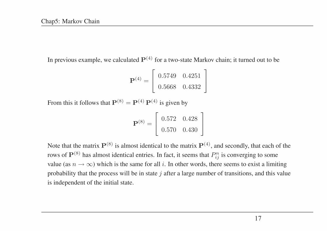
In previous example, we calculated P(4) for a two-state Markov chain; it turned out to be

P(4) =

⎡⎣ 0.5749 0.4251

0.5668 0.4332

⎤⎦

From this it follows that P(8) = P(4) P(4) is given by

P(8) =

⎡⎣ 0.572 0.428

0.570 0.430

⎤⎦

Note that the matrix P(8) is almost identical to the matrix P(4), and secondly, that each of therows of P(8) has almost identical entries. In fact, it seems that Pn

ij is converging to somevalue (as n → ∞) which is the same for all i. In other words, there seems to exist a limitingprobability that the process will be in state j after a large number of transitions, and this valueis independent of the initial state.

1917

Chap5: Markov Chain

Steady-state matrix

• The steady-state probabilities are average probabilities that the system will be in acertain state after a large number of transition periods.

• The convergence of the steady-state matrix is independent of the initial distribution.

• Long-term probabilities of being on certain states

limn→∞P(n) = π

2018

Chap 5: Markov Chain

�0P00 +��1P10 +��2P20 +�…�+�KPK0 =��0�0P01 +��1P11 +��2P21 +�…�+�KPK1 =��10 01 1 11 2 21 K K1 1

�0P0K +��1P1K +��2P2K +�…�+�KPKK =��K

19

�0 +��1 +��2 +�…�+�K =�1

Chap5: Markov Chain

• The limiting probability πj that the process will be in state j at time n also equals thelong-run proportion of time that the process will be in state j.

• Consider the probability that the process will be in state j at time n + 1

P (Xn+1 = j) =∞∑

i=0

P (Xn+1 = j|Xn = i)P (Xn = i) =∞∑

i=0

Pij P (Xn = i)

Now, if we let n → ∞, the result of the theorem follows.

• If the Markov chain is irreducible, then πj is interpreted as the long run proportion oftime the Markov chain is in state j.

2220

Chap5: Markov Chain

Illustrative example

Example 8: Consider Example 1, in which we assume that if it rains today, then it will rain

tomorrow with probability α; and if it does not rain today, then it will rain tomorrow withprobability β. If we say that the state is 0 when it rains and 1 when it does not rain, then thelimiting probability π0 and π1 are given by

π0 = απ0 + βπ1

π1 = (1 − α)π0 + (1 − β)π1

π0 + π1 = 1

which yields that

π0 =β

1 + β − απ1 =

1 − α

1 + β − α

For example, if α = 0.7 and β = 0.4, then the limiting probability of rain is π0 = 47 = 0.571.

2321