Markov-switching dynamic factor models in real time�

Maximo Camacho

Universidad de Murcia

mcamacho@um.es

Gabriel Perez-Quiros

Banco de España and CEPR

gabriel.perez@bde.es

Pilar Poncela

European Commission, Joint Research Centre and Universidad Autónoma de Madrid

pilar.poncela@ec.europa.eu

Abstract

We extend the Markov-switching dynamic factor model to account for some of the

speci�cities of the day-to-day monitoring of economic developments from macroeco-

nomic indicators, such as mixed-sampling frequency and ragged-edge data. First, we

evaluate the theoretical gains of using promptly available data to compute probabili-

ties of recession in real time. Second, we show how to estimate the model that deals

with unbalanced panels of data and mixed frequencies and examine the bene�ts of this

extension through several Monte Carlo simulations. Finally, we assess its empirical

reliability to compute real-time inferences of the US business cycle and compare it

with the alternative method of forecasting the probabilities of recession from balanced

panels.

Keywords: Business Cycles, Output Growth, Time Series.

JEL Classi�cation: E32, C22, E27

�We are indebted to Marcelle Chauvet for k ind ly sharing part of the real-tim e data vintages used in the empirica l app lication . We

thank the ed itor, the asso ciate ed itor and two anonymous rev iewers for their comments. Part of th is pap er was w ritten while the th ird

author was visiting the Bank of Spain . F inancia l support from the Spanish governm ent, contract grants ECO2015-70331-C2-1-R and

ECO2016-76178-P (M INECO/FEDER), and 19884/GERM/15 (G roups of Excellence, Fundación Séneca, and Science and Technology

Agency), is gratefu lly acknow ledged . Any errors are our resp onsib ility. The view s in th is pap er are those of the authors and do not

represent the view s of the Europ ean Comm ission , the Bank of Spain or the Eurosystem . Codes and data that rep licate the resu lts

can b e downloaded from the authors� websites.

1

1 Introduction

The 2008-2009 was the most sustained economic slump that the United States has weath-

ered since World War II. One of the lessons that this Great Recession left for economists

was that policymakers and business people, who had become accustomed to the serene con-

ditions of the Great Moderation, have dramatically increased their interest in determining

as quickly as possible whether the economy has su¤ered from a business cycle phase shift.

In this context, time-series models, which are able to automate the increasing complexity

of the signal extraction problem in economics, help the economic agents to perform and

update their real-time views of the developments in economic activity. These models deal

with economic indicators that share the two properties of the business cycle documented

early by Burns and Mitchell (1946): their signals about economic developments are spread

over the di¤erent aggregates and they exhibit business cycle asymmetries.

Diebold and Rudebusch (1996) were the �rst to suggest a uni�ed model that captures

these two business cycle features from a set of economic indicators. They argued that

comovements among the individual economic indicators can be modelled by using the

linear coincident indicator approach described in Stock and Watson (1991), while the

existence of two separate business cycle regimes can be modelled by using the Markov-

switching speci�cation advocated by Hamilton (1989). Integrating these approaches, Kim

and Yoo (1995), Chauvet (1998) and Kim and Nelson (1998) combined the dynamic-factor

and Markov-switching frameworks to propose di¤erent versions of statistical models which

simultaneously capture both comovements and regime shifts. Camacho, Perez-Quiros and

Poncela (2015) �nd that the fully non-linear multivariate speci�cation outperforms the

�shortcut�of using a linear factor model to obtain a coincident indicator which is then used

to compute the Markov-switching probabilities. Recently, Chauvet and Hamilton (2006),

Chauvet and Piger (2008), and Hamilton (2011) have examined the empirical reliability

of these models in computing real-time inferences of the US business cycle states.

An important limitation of these Markov-switching dynamic factor models (MS-DFM)

is that they were originally designed to deal with balanced panels of business cycle indi-

cators. This crucial assumption means MS-DFM exhibit two drawbacks when applied to

2

the (timely) day-to-day monitoring of economic activity in real time. The �rst drawback

is that the typical lack of synchronicity in the �ow of macroeconomic information implies

that some indicators are published with a time delay, which requires dealing with unbal-

anced panels of data. Not accounting for this publication pattern would imply that the

users of traditional MS-DFM who develop early assessments of economic developments

from balanced panels of data will unavoidably incur one of the two following substantial

costs. The �rst cost appears when the forecasts are made from the latest available balanced

panel. In this case, the forecasts lose the latest and most valuable information contained

in the promptly issued indicators at the time of the assessments. The second cost is that of

being late when the analysts decide to wait until all the business cycle indicators become

available and the inferences, which are then actually referred to the past. A signi�cant

example of this limitation is the two-month lag in the reporting real-time recession prob-

ability chart released by the St Louis Fed, which uses the MS-DFM originally developed

in Chauvet (1998).

The second drawback of standard MS-DFM is that they relate variables sampled at

the same frequency. In practice, although some of the macroeconomic indicators that

are observed to infer business cycle states are sampled quarterly, some others, potentially

useful in real-time inferences, are often sampled at a higher frequency. For example,

the National Bureau of Economic Research (NBER) Dating Committee acknowledges

that recessions are de�ned as signi�cant declines in economic activity normally visible

in real Gross Domestic Product (GDP), which is available quarterly, and real income,

employment, industrial production, and wholesale-retail sales, which are available monthly.

In this paper, we examine the extent to which the incoming information provided

by new releases of promptly published economic indicators, which potentially sampled at

di¤erent frequencies, could help to improve the real-time inference about the business cycle.

Using a theoretical MS-DFM, we show the extent to which inferences about the state of the

economy can be improved upon by including early available indicators. Interestingly, we

�nd that the improvements in performance depend on the factor loadings, the idiosyncratic

variances, the dynamics of the common factor, and the di¤erence between the means in

the business cycle states.

3

Then, we extend the MS-DFM to allow economic agents that track business cycle

developments in real time to use whatever business cycle economic indicator, regardless of

their publication delays, and regardless of whether they are sampled monthly or quarterly.

Based on a Markov-switching extension of the linear dynamic factor model proposed by

Mariano and Murasawa (2003), our procedure deals with missing observations by using

a time-varying nonlinear Kalman �lter. Whenever the data is not observed, the missing

observations are replaced by random draws from a variable whose distribution cannot

depend on the parameter space that characterizes the Kalman �lter. The corresponding

row is then skipped in the Kalman recursion and the measurement equation for the missing

observation is set to the random choice.

By means of several Monte Carlo experiments, we measure the magnitude of the gains

of using our extension to compute business cycle inferences. We show that our proposal

outperforms MS-DFM that requires balanced panels, especially when the forecasting hori-

zon increases, when the two states are well separated, and when the variance and the

inertia of the idiosyncratic components are low. Finally, we use a real-time data set to

show that our extension of the MS-DFM leads to signi�cant improvements in computing

real-time business cycle inferences compared with forecasting from balanced and/or lagged

panels of indicators using the four constituent monthly series of the Stock-Watson coin-

cident index. Notably, we show that adding GDP does not seem to produce signi�cant

improvements in this setting.

The structure of this paper is organized as follows. Section 2 assesses the real-time

features of the data�ow within a factor model framework. Section 3 examines the relative

performance gains of dealing with ragged-edge data through a Monte Carlo experiment.

Section 4 illustrates these results for US real-time data. Section 5 concludes.

2 The model

2.1 Model features

Our framework is the single-index Markov-switching dynamic factor model proposed in

the mid-nineties by Kim and Yoo (1995), Chauvet (1998), and Kim and Nelson (1998),

4

which incorporates both comovements and business-cycle shifts into a statistical model.

The model postulates that a vector of N economic indicators, yt = (y1;t; :::; yN;t)0, which

are hypothesized to move contemporaneously with the overall economic conditions, can be

decomposed as the sum of two components. The �rst component is a linear combination

of r unobserved factors, f t = (f1;t; :::; fr;t)0, that accounts for the common comovements.

The second component is the N �1 time series vector ut, that represents the idiosyncratic

movements in the series. This suggests the formulation:

yt = � f t + ut; (1)

where� is the N�r factor loading matrix and ut is the vector of idiosyncratic components.

To account for the business cycle asymmetries, it is assumed that the dynamic behavior

of the common factors is governed by an unobserved regime-switching state variable, st.

Within this framework, one can label st = 0 and st = 1 as the expansion and recession

states at time t. In addition, it is standard to assume that the state variable evolves

according to an irreducible 2-state Markov chain whose transition probabilities are de�ned

by

p(st = jjst�1 = i; st�2 = h; :::; It�1) = p(st = jjst�1 = i) = pij ; (2)

where i; j = 0; 1, and It is the information set up to period t, i.e., fy1; :::;ytg. We

assume that the vector of common factor follows an autoregressive process with switching

intercept,

f t = �st + �1f t�1 + :::+ �pf t�p + at; (3)

where at is white-noise with variance �a, which is independent of st. The main identifying

assumption in the model expresses the core notion that the comovements of the multiple

time series arise from the common component. This is achieved by assuming that ut and

f t are mutually uncorrelated at all leads and lags.1

Each element ui;t of the idiosyncratic error ut = (u1;t; :::; uN;t)0 is assume to follow an

autoregressive process of order pi

ui;t = i;1ui;t�1 + :::+ i;piui;t�pi + �i;t; (4)

1Additional identifying restrictions, which are required to estimate the model, are not discussed in this

theoretical section.

5

being f�i;tg a white noise process with variance �2i;st . In matrix form, the dynamics of the

idiosyncratic component is

ut = 1ut + :::+Put�P + �t; (5)

where j = diag( 1;j ; :::; N;j), P = max(p1; :::; pN ), and var(�t) = diag(�21;st ; :::; �2N;st

).2

2.2 Theoretical gains of using promptly available data

To facilitate the theoretical analysis, in this section we consider several simplifying as-

sumptions. The �rst one is that we rely on publication lags of only one month. Therefore,

we focus on considering the gains of using new partial information arriving at t+ 1. The

second simplifying assumption is that the vector of idiosyncratic components, ut, is a

multivariate white noise with variance-covariance matrix �u;st . However, we do maintain

the assumption that this variance-covariance matrix can depend on the state. Third, the

maximum lag length for the autoregressive model of the factors is p = 1.3

Then, we focus on computing inferences about the business cycle regime at t+1, that

is, computing prob(st+1 = j) conditional on di¤erent information sets. Let us assume that

all the indicators are collected up to time t, yt. However, we assume that only a subset of

promptly published indicators, collected in the subvector yk;t+1, with k < N , is available

at t + 1. If we are restricted to using balanced panels, as in traditional MS-DFM, this

forced us to use only the information It, obtained before the �rst arrival of new information

at t+ 1. Therefore, our guess of the probability of being in a certain state at t+ 1 is the

one step ahead forecast of the �ltered probability prob(st = jjIt):

prob(st+1 = jjIt) =1Xi=0

prob(st = ijIt)pij : (6)

However, the extension of MS-DFM proposed in this paper allows for incorporating

the information provided by yk;t+1 as it arrives. In this case, the inference of being in a

2Assuming that the idiosyncratic components are uncorrelated in cross-section is a necessary condition

to identify the common factors in small scale factor models (Barhoumi et al., 2014). In large scale models

(N !1), the assumption is that idiosyncratic errors are only weakly correlated.3The extensions to larger reporting lags, serially correlated idiosyncratic components, and further lags

in the autoregressive model of the common factor are conceptually easy, although they would complicate

computations considerably.

6

certain state at t+ 1 can be obtained as

prob(st+1 = jjIt;yk;t+1) =f(yk;t+1jst+1 = j; It)

f(yk;t+1jIt)prob(st+1 = jjIt): (7)

Using the new information will be useful if it raises the ability to increase the true signals.

This implies that it should increase the probability of a given state when the economy

is actually in that state. For instance, let us assume that the economy is in recession

at t + 1, i.e., st+1 = 1,4 and that 0 < prob(st+1 = jjIt) < 1:5 Hence, from (7), the

partial information provided by yk;t+1 is helpful to reduce false signals when prob(st+1 =

1jIt;yk;t+1) > prob(st+1 = 1jIt), which occurs whenever

f(yk;t+1jst+1 = 1; It) > f(yk;t+1jIt): (8)

Using the total law of probabilities, if st+1 = 1 the condition in (8) would be

f(yk;t+1jst+1 = 1; It) > f(yk;t+1jst+1 = 1; It)prob(st+1 = 1jIt)+f(yk;t+1jst+1 = 0; It)prob(st+1 = 0jIt);

(9)

which, rearranging terms, leads to

f(yk;t+1jst+1 = 1; It) > f(yk;t+1jst+1 = 0; It): (10)

In practice, these two density functions may overlap and the condition does not hold

for all possible values of yk;t+1. In these cases, even when the true state is st+1 = 1,

it might happen that for some (relatively high) values of yk;t+1; f(yk;t+1jst+1 = 1; It) <

f(yk;t+1jst+1 = 0; It). This might lead to a false signal detection since the probability

for st+1 = 1 decreases when yk;t+1 is observed. Accordingly, the usefulness of yk;t+1

to compute business cycle inferences should be evaluated on average. Taking natural

logarithms, the condition in (10) implies that using the incoming information helps in

inferring recession probabilities in actual recessions when

ln f(yk;t+1jst+1 = 1; It)� ln f(yk;t+1jst+1 = 0; It) > 0: (11)

4 If we assumed that the true state is st+1 = 0, we would obtain symmetric results for the probability

of expansion.5 It is straightforward to check that if prob(st+1 = jjIt) = 1, then prob(st+1 = jjIt;yk;t+1) = 1; j = 0; 1.

7

Now, taking into account all possible outcomes of yk;t+1 for the true state st+1 = 1, the

expected value of the di¤erence between the two conditional densities under conditional

Gaussianity is given by the Kullback-Leibler divergenceZlnf(yk;t+1jst+1 = 1; It)f(yk;t+1jst+1 = 0; It)

f(yk;t+1jst = 1; It)dyk;t+1; (12)

where we use the notation in Cover and Thomas (2006) for the multiple integral. The

next proposition, which is based on the concept of conditional entropy, quanti�es the

potential advantage of adding the advanced business cycle signals provided by the promptly

published indicators yk;t+1.

Proposition 1 Assume the factor model given by (1), (2) and (3), where the vector of

idiosyncratic components, ut is multivariate white noise, and the lag length of the factors

dynamics is p = 1, with autoregressive matrix �. Under conditional Gaussianity, the gain

in t+ 1 from observing the subvector of k variables yk;t+1is given by the Kullback-Leibler

divergence of f(yk;t+1jst+1 = 1; It) with respect to f(yk;t+1jst+1 = 0; It)

KL =1

2ln(2�)k (j�0j � j�1j)+

1

2tr��1�

�10

�� k2+1

2(f1 � f0)0 �0k��10 �k (f1 � f0) ; (13)

where f i = E�f t+1jst+1 = i; It

�, �i = E

�(yk;t+1 � �kf i)(yk;t+1 � �kf i)0jst+1 = i; It

�,

i = 0; 1 and �k is the k � r submatrix of factor loadings associated to yk;t+1.

Proof: The proof is given in the Appendix.

This expression suggests that using the �rst arrival of new information collected in

yk;t+1 is expected to raise the ability to increase the true business cycle signals when the

di¤erence in the expected value of the common factors and the between the within-state

covariance matrices of the early available indicators are large.

As, for example, in Chauvet and Hamilton (2006), Chauvet and Piger (2008), and

Hamilton (2011), empirical applications of MS-DFM typically rely on the assumptions

that there is only one common factor and that the variances are state-independent. The

next corollary focuses in this case.

Corollary 2 For the one-factor model with state-independent variances, �u = diag��21; �

22; :::; �

2N

�and � = (�1; :::; �N )

0, the Kullback-Leibler divergence of f(yk;t+1jst+1 = 1; It) with respect

8

to f(yk;t+1jst+1 = 0; It) simpli�es to

KL =(�0 � �1)2

2

0@ 1Pki=1

�2i�2i

+ �2Ptjt + �2a

1A�1

; (14)

where Ptjt = E�ft � ftjtjIt

�2:

Proof: The proof is given in the Appendix.

This expression implies that if there are separate business cycles regimes in the sense

that �1 6= �0 and �2a <1, and the common factor is not weak (as in Lam, Yao and Bathia,

2011) with respect to the early published indicators, that is �k 6= 0k�1, the divergence is

strictly positive. This implies that the incoming information provided by a new release of

k economic indicators is always expected to be useful to improve upon the inference about

the business cycle at time t+ 1 with respect to using only the information up to t.

In addition, the expression quanti�es the magnitude of the change in the conditional

entropy and reveals that the averaged gains of using the business cycle information content

of yk;t+1 will depend on several parameters. First, the information content of yk;t+1 in-

creases with the di¤erence between the within-state means, �0��1, because the states are

more easy to identify from the information provided by the new data. Second, the expres-

sion shows that the greater the signal signal-to-noise ratios, �2i

�2i, the larger the expected

gains to infer the business cycle regimes from observing yk;t+1. Third, the divergence

diminishes with the variance of the common factor, �2a.

Finally, the conditional entropy decreases as j�j increases because �2Ptjt is always pos-

itive. Therefore, the serial dynamics in the common factor make harder the identi�cation

of the business cycle phases because this makes the common factor more variable relative

to the di¤erence in means across regimes. Also, Ptjt is increasing in � (see, Poncela and

Ruiz, 2015) and, therefore, the more persistent the common factor is (in the sense that

� ! 1), more di¢ cult it is to separate expansions from recessions. Then, for a better

identi�cation of the business cycle phases, from now on we will assume that p = 0 in (3).

In the case of idiosyncratic errors with serial correlation, the integral in (12) does not

have a closed form solution since it involves computing the Kullback-Leibler divergence

of mixtures of Gaussians (see, for instance, Michalowicz, Nichols and Bucholtz, 2008, or

9

Cui, 2016, among many others). We will illustrate the value of new information through

several simulations and an empirical application in the following sections.

3 Extending the single-index MS-DFM

3.1 State space representation

In what follows, we will focus in the case of interest in our empirical application, the model

with just one common factor representing the aggregate economic activity. If we assume

that all indicators were always observed with no reporting lags and that the quarterly in-

dicators were sampled each month, the model can be cast into a state space representation

yt = Hht + �t; (15)

ht = Mst + Fht�1 + �t; (16)

with �t � N(0;R) and �t � N(0;Q).

Without loss of generalization, consider that only the �rst indicator is sampled quar-

terly. If it refers to stocks, it can easily be converted into monthly observations since they

simply refer to quantities which are measured at a particular time. If it refers to �ow

variables, Mariano and Murasawa (2003) propose a time aggregation which is based on

the notion that its quarterly growth rates, y1;t, are weighted averages of its (assumed to

be known) monthly past growth rates, xt:

y1;t =1

3xt +

2

3xt�1 + xt�2 +

2

3xt�3 +

1

3xt�4: (17)

For example, if the idiosyncratic components are autoregressive processes of order pi =

1, and if we assume p = 0 in (3), the matrices in the measurement equation (15) are yt =

(y1;t; y2;t; � � � ; yN;t)0, �t = 0N�1,R = 0N�N , ht = (ft; :::; ft�5; u1;t; :::; u1;t�5; u2;t; � � � ; uN;t)0,

and

H =

0BBBBBB@

�13

2�13 �1

2�13

�13

13

23 1 2

313 0 0 � � � 0 0

�2 0 0 0 0 0 0 0 0 0 1 0 � � � 0 0...

......

......

............

.......... . .

......

�N 0 0 0 0 0 0 0 0 0 0 0 � � � 0 1

1CCCCCCA : (18)

10

In this example, the matrices in the transition equation (16) are Mst = (�st ;00(N+9)�1)

0,

F =

0BBB@F11 05�5 05�N�1

05�5 F22 05�N�1

0N�1�5 0N�1�5 F33

1CCCA ; (19)

where

F11 =

0@ 01�4 0

I4 04�1

1A ; (20)

F22 =

0@ ( 1; 0; 0; 0) 0

I4 04�1

1A ; (21)

F33 = diag ( 2; :::; N ), and Q = diag��2a; :::; 0; �

21; 0; :::; 0; �

22; :::; �

2N

�.

The model can be estimated by maximum likelihood as follows. Let h(i;j;k;l;m)tjt�1 be the

one-period-ahead forecast of ht based on information up to period t � 1, given the path

(st�4 = i; st�3 = j; st�2 = k; st�1 = l; st = m) and let P(i;j;k;l;m)tjt�1 be its covariance matrix.

The prediction equations become

h(i;j;k;l;m)tjt�1 = Mst + Fh

(i;j;k;l)t�1jt�1

; (22)

P(i;j;k;l;m)tjt�1 = FP(i;j;k;l)

t�1jt�1F0 +Q; (23)

where h(i;j;k;l)t�1jt�1

is the estimation of ht�1 at time t � 1 with information up to time t � 1

if (st�4 = i; st�3 = j; st�2 = k; st�1 = l) and P(i;j;k;l)t�1jt�1

its covariance matrix, that will be

given in (27) and (28), respectively. The conditional one-step-ahead forecast errors are

u(i;j;k;l;m)tjt�1 = yt �Hh(i;j;k;l)tjt�1 and �(i;j;k;l;m)tjt�1 = HP

(i;j;k;l)tjt�1 H0+R is its conditional variance.

Hence, the log likelihood given (st�4 = i; st�3 = j; st�2 = k; st�1 = l; st = m) can be

computed at each t as

l(i;j;k;l;m)t = �1

2ln�2�����(i;j;k;l;m)tjt�1

����� 12u(i;j;k;l;m)0tjt�1

��(i;j;k;l;m)tjt�1

��1u(i;j;k;l;m)tjt�1 : (24)

The updating equations become

h(i;j;k;l;m)tjt = h

(i;j;k;l;m)tjt�1 +K

(i;j;k;l;m)t u

(i;j;k;l;m)tjt�1 ; (25)

P(i;j;k;l;m)tjt = P

(i;j;k;l;m)tjt�1 �K(i;j;k;l;m)

t HP(i;j;k;l;m)tjt�1 ; (26)

11

where the Kalman gain, K(i;j;k;l;m)t , is de�ned asK(i;j;k;l;m)

t = P(i;j;k;l;m)tjt�1 H0

��(i;j;k;l;m)tjt�1

��1.

In addition, maximizing the exact log likelihood function of the associated nonlinear

Kalman �lter is computational burdensome since at each iteration, the �lter produces a

2-fold increase in the number of cases to consider. The solution adopted in this paper is

based on collapsing some terms of the former �lter as proposed by Kim (1994) and used

by Kim and Yoo (1995) and Chauvet (1998):

h(j;k;l;m)tjt

=

1Xi=0

p (st�4 = i; st�3 = j; st�2 = k; st�1 = l; st = mjIt)h(i;j;k;l;m)tjt

p (st�3 = j; st�2 = k; st�1 = l; st = mjIt); (27)

P(j;k;l;m)tjt

=

1Xi=0

p (st�4 = i; st�3 = j; st�2 = k; st�1 = l; st = mjIt)�(i;j;k;l;m)tjt

p (st�3 = j; st�2 = k; st�1 = l; st = mjIt); (28)

where �(i;j;k;l;m)tjt = P

(i;j;k;l;m)tjt +

�h(j;k;l;m)tjt

� h(i;j;k;l;m)tjt

��h(j;k;l;m)tjt

� h(i;j;k;l;m)tjt

�0.

3.2 Missing data

In practice, imposing that all variables are always observed is quite unrealistic. Performing

real-time inferences on the business cycle typically requires exploitation of the information

of early available indicators, which could be sampled at di¤erent frequencies, mainly quar-

terly and monthly. The presence of ragged-edge data generate missing data at the end of

the sample while the missing data appear in quarterly indicators because their �gures are

only available once every three monthly outcomes.

In linear contexts, Mariano and Murasawa (2003) show that the system of state-space

equations remains valid with missing data after a subtle transformation. These authors,

�ll in the missing observations with random numbers that are extracted from a random

variable whose distribution is independent of the model parameters. Then, the measure-

ment equation is modi�ed to get that the Kalman �lter skips the random numbers. From

a computational point of view, the parameters that maximize the likelihood and the in-

ferences about the business cycle states are achieved as if all the variables were observed.

The procedure can be adapted to Markov-switching models easily. Without loss of

generalization, let us focus on dealing with missing data only in the t-th observation of

12

one monthly indicator, yN;t, which is the last component of the vector of time series yt.

Let � be the vector that includes all the unknown model parameters. Let us de�ne the

variable

y+i;t :=

8<: yi;t for i = 1; :::; N � 1

zt for i = N; (29)

where zt is a random variable whose distribution is independent of � and st; for instance,

zt � N(0; �2z). Let f(zt;�) be the density function of zt, which depends on a vector of

parameters �.

Accordingly, no modi�cations of the nonlinear algorithm used to estimate MS-DFM

are required, apart from considering a time varying Kalman �lter to zero out the missing

observations. Let Rii be the variance of the i-th element of yt, let Hi be the i-th row of

the matrixH which has & columns, and let 01& be a row vector of & zeroes. In our example,

the measurement equation can be replaced by the following expressions

H+it :=

8<: Hi for i = 1; :::; N � 1

01& for i = N; (30)

�+it :=

8<: 0 for i = 1; :::; N � 1

zt for i = N; (31)

R+iit :=

8<: 0 for i = 1; :::; N � 1

�2z for i = N: (32)

This trick leads to a time-varying state space model with no missing observations so the

nonlinear �lter can be directly applied to y+, H+, �+t , and R+.

4 Monte Carlo simulations

We generate a total ofM = 1000 sets of N idiosyncratic components umt of length T , where

T = 600, which is about the lag length of the monthly indicators used in our empirical

application. Without loss of generality, the time series are generated with equal variances

�2i = �2 across time series. However, to examine the e¤ect of the quality of the indicators in

the forecasting accuracy, the series are generated with the same but increasing idiosyncratic

variance �2 of 0:5, 1:5, and 4:5. The dynamics of these idiosyncratic components follow

13

autoregressive processes of order one with autoregressive parameters equal to i;1 = =

0:3 for all time series. To evaluate the e¤ect of the persistence on the inferences, we also

perform simulations with = 0:6.

In addition, we generate M = 1000 dummy variables bmt of zeroes and ones of length

T which are used to simulate di¤erent sequences of expansions (bmt = 0) and recessions

(bmt = 1). To ensure that the dummies share the US business cycle properties, bmt follows

Markov chains with p00 = 0:98 and p11 = 0:9.6 Then, we generate M = 1000 common

factors, fmt , that follow Markov-switching processes given by (3) with p = 0 . In this case,

the business cycle sequences bmt to classify the business cycle states and the within state

means are set to �0 = 1 and �1 = �1. Then, to examine how the di¤erence between the

within-state means a¤ects the results, �0 is increased to 2. Finally, setting �2a = 1 and

using factor loadings equal to one for all the series, we add the idiosyncratic components

to the switching mean factors to generate M = 1000 sets of N time series fymt gTt=1.

To examine the e¤ects of dealing with ragged-edge data in computing the real-time

business cycle inferences, we assume that an analyst faces the forecasting problem with one

publication lag in four out of the set of N indicators used in the analysis. For completeness,

the simulations are also computed when these four indicators exhibit two publication lags

and the role of N is addressed by using a total number of indicators of 5 and 7.

We consider that the analyst wants to infer the probability of recession at T from

the set of N indicators under two di¤erent scenarios. The �rst scenario consists of using

traditional MS-DFM to infer recession probabilities at T with the (as large as possible)

amount of information disposable at T . In this case, the forecasts are computed from

the latest available balanced panel of N indicators. Hence, she has to compute one-

step-ahead forecasts to obtain prob(sT = 1jIT�1) and two-step-ahead forecasts to obtain

prob(sT = 1jIT�2) from the set of N indicators when there are one and two periods of

publication lags, respectively.

The second scenario consists of using our extension of MS-DFM that is able to deal

6According to the NBER Business Cycle Dating Committee, these transition probabilities coincide

with the percentage of months classi�ed as expansions that are followed by expansions and the percentage

of quarters classi�ed as recessions that are followed by recessions in the period used in the empirical

application 1967:02-2017:03.

14

with ragged-edge data. In this case, the inferences can be computed from the set of N

indicators even when four of them are not available at T , i.e., the analyst can compute

prob(sT = 1jI+T ), where I+T refers to the information provided by the set of N�4 promptly

published indicators up to T and the 4 delayed indicators up to T �h, with h = 1; 2, when

the publication lag is of one and two months, respectively. In this case, the variance of

the N � 4 indicators that are published timely is 1:5, and the variance of the 4 delayed

indicators is allowed to change from 0:5 to 1:5, and 4:5

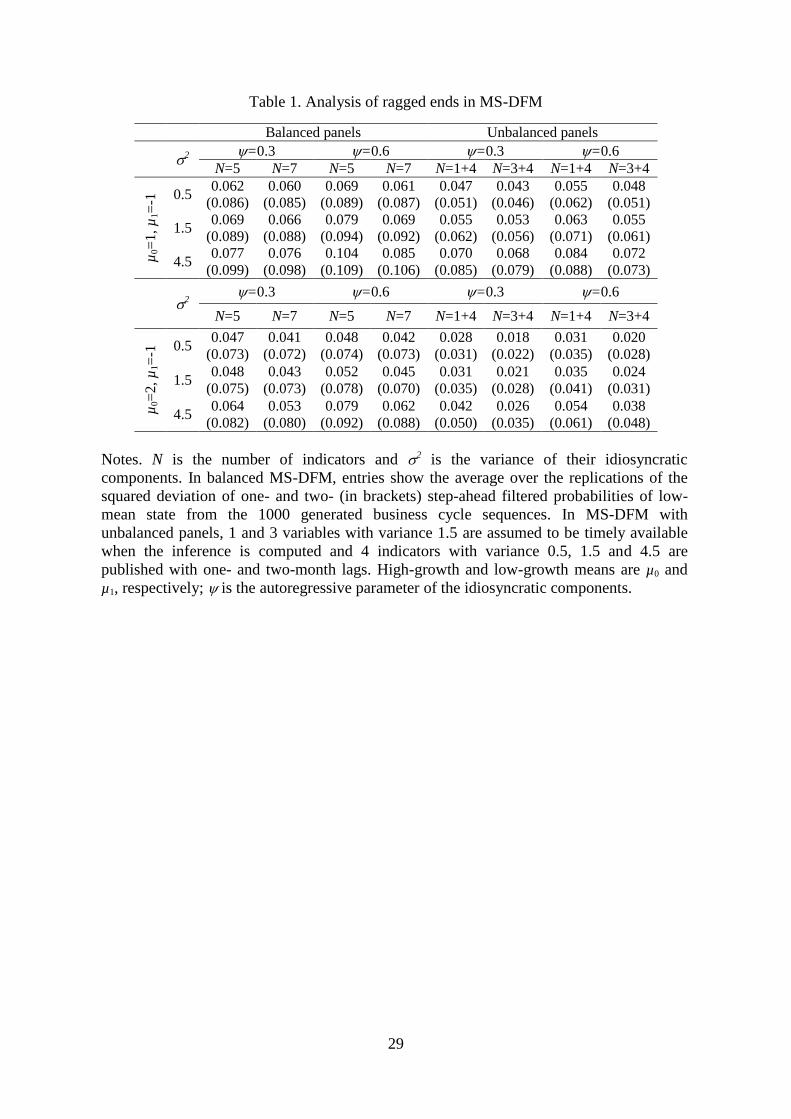
For each m-th replica, we quantify the ability of these procedures to detect the actual

state of the business by computing the Forecasting Quadratic Probability Score (FQPS):

FQPSi =1

M

MXm=1

(pmT;i � bmT )2: (33)

In this expression, i = I in the case of traditional MS-DFM that forecast from the latest

available balanced panel, and pmT;i = prob(sT = 1jIT�1) or pmT;i = prob(sT = 1jIT�2)

in the cases of one-step-ahead or two-step-ahead forecasts. By contrast, i = II in the

case of our extension of MS-DFM, which is able to deal with missing observations, and

pmT;i = prob(sT = 1jI+T ). Hence, the measure is the average over the M replications of the

squared deviation of the di¤erent types of inferences from the generated business cycles.

Table 1 displays the FQPS statistics when four indicators exhibit one and two (in

brackets) publication lags. Notably, the table shows that using the incoming information

as it is available always helps to increase the accuracy of the models. For example, let

us focus on the case of computing inferences from N = 5 indicators when four of them

exhibit a one-period publication delay in the case �2 = 1:5. When the one-step ahead

probability forecasts are computed from the balanced set of �ve indicators with one lag of

publication delay, the inferences computed from the traditional MS-DFM exhibit FQPSI

of 0:069. However, the the MS-DFM that allows ragged-edge data uses one timely available

indicator and four indicators with one publication lag to substantially improve the business

cycle inferences, reaching a fall in the FQPSII to 0:055. In addition, the accuracy gains

of accounting for ragged-edge data increase when the publication delay is two months

(FQPSI of 0:089 vs FQPSII of 0:062, in brackets).

Notably, the sharp increases in the forecasting accuracy detected below are achieved

15

by using only one timely published indicator. When the number of promptly available

indicators increases, the inferences computed from the model that accounts for ragged-edge

data also outperform those computed from the model that computes probability forecasts

from the balanced sets of indicators (FQPSI of 0:064 vs FQPSII of 0:053), especially

when the indicators exhibit larger publication delays (FQPSI of 0:088 vs FQPSII of

0:056).

The entries displayed in Table 1 show that the ability to compute business cycle in-

ferences from unbalanced panels crucially depends on the signal-to-noise ratio of the early

available indicators. Regardless of the forecasting scenario, FQPS rises when the variance

of the idiosyncratic component increases from 0:5 to 1:5 and 4:5, and the relative gains of

using unbalanced panels diminish as the signal-to-noise ratio increases. In addition, the

table shows that higher di¤erences of within-state means, from �0 = 1 to �0 = 2 for a �xed

�1 = �1, improve the performance of the models to compute business cycle inferences.

Interestingly, the improvements are signi�cantly higher for the model that uses timely

available indicators. Finally, the table also shows that the persistence of the idiosyncratic

component of the time series tends to diminish the performance of the models.

5 Empirical application

The purpose of this section is to examine the relative empirical performance of our modi�ed

MS-DFM, which is able to deal with ragged-edge data and mixed frequencies, with respect

to traditional MS-DFM, which are restricted to use balanced panels of data.

5.1 In-sample analysis

The four monthly indicators used in the empirical analysis are industrial production index,

nonfarm payroll employment, personal income less transfer payments and real manufac-

turing and trade sales. Although the latest available data set was downloaded on June,

15th 2017, the balanced panel of four monthly indicators only includes data from 1967:01

to 2017:03, because income is only available up to April 2017 and sales is only available

up to March 2017.

16

Since the seminal proposal of Diebold and Rudebusch (1996), the behavior of these

series is assumed to follow the comovements and asymmetries that Burns and Mitchell

(1946) designated as the key business cycle features. Following their lines, we �t a MS-

DFM to the balanced panel of one hundred times the change in the natural logarithm of

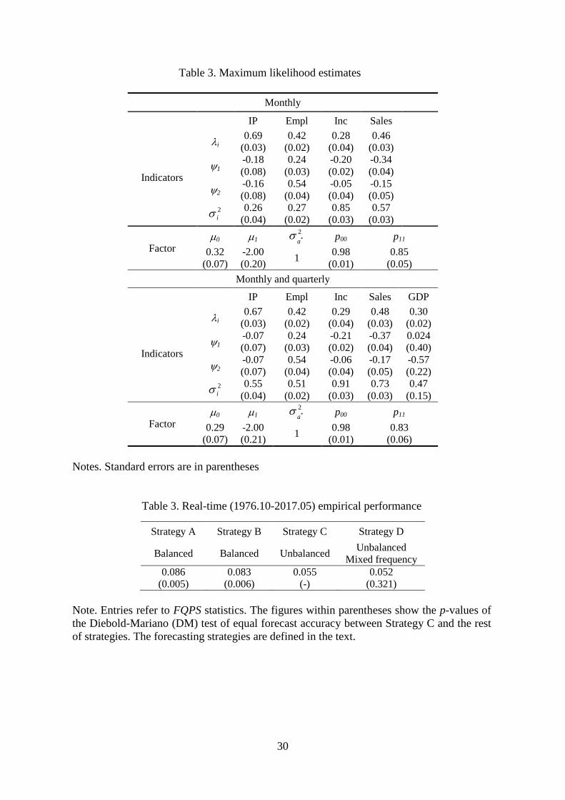
these four macroeconomic variables.7 The maximum likelihood estimates of this monthly

model, which are displayed in the top panel of Table 2, show that the estimates of the

signal-to-noise ratios agree with the magnitudes used in the simulation experiments. In

particular, the highest values of the signal-to-noise ratios are achieved by industrial pro-

duction, the medium values by employment, and the lowest values by sales and income. In

addition, the estimates show that the factor loadings are positive and statistically signi�-

cant. Hence, the indicators are positively correlated with the estimated common factor.

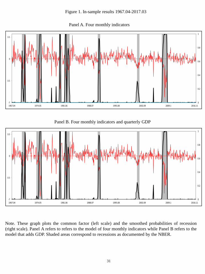
In line with this statement, Figure 1 shows that the coincident index describes a

behavior that closely agrees with the NBER-designated US business cycles.8 In terms of

ROC classi�cation, the common factor capture the state of the US business cycle with

AUROC values fairly close to the near-perfect classi�cation ability value of one, with

AUROC of 0:94. The magnitude of the AUROC is comparable to that obtained by Berje

and Jorda (2011) for two well-known indices of the US business conditions: the Chicago

Fed National Activity Index (CFNAI) and the Aruoba, Diebold, and Scotti (2009) Business

Conditions Index maintained by the Federal Reserve Bank of Philadelphia.9

Notably, the maximum likelihood estimates reported in the top panel of Table 2 also

show that the transition probabilities are very persistent (p00 = 0:98; p11 = 0:85) and that

the within-state means are separated from each other (�0 = 0:32; �1 = �2:00). Panel

A of Figure 1, which plots the probabilities that the coincident indicator is in recession

based on currently available information along with shaded areas that represent periods

7 In line with Stock and Watson (1991), all the linear autoregressive processes are estimated with two

lags. Folloing Camacho and Perez Quiros (2007), the nonlinear factor is estimated with no lags.8 In the empirical analysis, we take it as given that the NBER correctly identi�es the dates of business

cycle turning points.9The common factor of a linear DFM has AUROC=0:94. Although MS-DFM exhibits similar perfor-

mance in terms of ROC classi�cation, it has the advantage of computing the probability that the common

factor is in recession.

17

dated as recessions by the NBER, shows that the smoothed probabilities are in striking

agreement with the professional consensus as to the history of US business cycles.

Our extension of MS-DFM allows us to obtain nonlinear estimates and business cycle

inferences from a data set that contains business cycle indicators with monthly and quar-

terly frequencies. In addition to the four monthly indices, we include the growth rate of

U.S. quarterly real GDP from 1967:1 to 2017:1. The bottom panel of Table 2 shows that

the maximum likelihood estimates that refer to the monthly series and the common factor

are similar to the estimates obtained when GDP was not included in the model. The

dynamics of the common factor, which is plotted in Panel B of Figure 1, is also in close

agreement with the dynamics of the estimated common factor obtained from the model

that excludes GDP. An interesting result is that its AUROC is also 0:94, which reveals

that quarterly GDP does not seem to improve the in-sample classi�cation ability of the

four monthly indicators.

5.2 Real-time analysis

The previous in-sample analysis has been conducted with data of the most recent vintage.

However, the real-time data could be less helpful in monitoring the real activity than the

in-sample evaluations developed in the previous section using �nally revised data sets. On

the one hand, it has been argued in the related literature (see, for example, Diebold and

Rudebusch, 1991) that the good performance of the end-of-sample vintages in examining

the empirical performance of econometric models may be spurious, in the sense that the

data actually available in real time include economic time series that are subject to revision

and that the economic relationships may change over time. In our case, the measures

of production, employment and sales are typically subject to substantial revisions that

sometimes occur years after the o¢ cial �gures are �rstly released. On the other hand, the

in-sample analysis does not allow the researchers to evaluate the e¤ects of managing the

lack of synchronicity that characterizes the daily �ow of macroeconomic information in

the early assessments of the economic developments.

To perform a more realistic assessment of the actual empirical reliability of the MS-

DFM, we evaluate their real-time performance at tracking the US business cycles in real

18

time through a data set that consists of real-time vintages obtained from January 15, 1976

to June 15, 2017. That is, the inferences are computed at each month t over the past four

decades that covers the period December, 1976 to May, 2011 by using only the data that

would have been available at the middle of the month that follows the particular month

in which the inference is computed.10 Hence, the real-time analysis does not include the

data revisions that were not available at the time the model would have been used and

has to manage with incomplete data sets at the time of each inference.

To clarify understanding, let us describe the stylized publication calendar of the eco-

nomic indicators used in the real-time analysis. At the end of month t, Industrial Pro-

duction is published on the 15th of the month t+ 1; Non-farm Employees is published on

the 8th of the month t + 1, Real Personal Income is published on the 27th of the month

t+1, and Real Manufacturing, Trade Sales is published on the 27th of the month t+2.11

In addition, GDP is published on the 15th of t+2, whenever t is March, June, September

or December. To simplify the real-time analysis, we consider that the real-time inferences

are computed on the 15th of each month, where employment and industrial production

are available for the previous month. On this day, of month t+1, we infer the probabilities

of being in a recession at t, with industrial production and employment up to t, personal

income up to t� 1, and real sales up to t� 2.

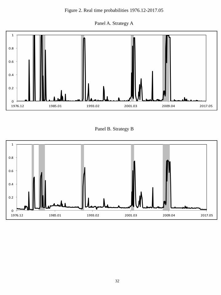
According to our theoretical and Monte Carlo results, the business cycle probabilities

are inferred from di¤erent alternative strategies. The �rst two strategies consist of com-

puting inferences from traditional MS-DFM which can only account for balanced data sets.

This implies that the model cannot use either quarterly series or the information provided

by the early published indicators since the data set must be constrained to �nish at t� 2.

Within this strategy, called strategy A, the inferences computed at t � 2 are considered

as the prevailing business cycle conditions for period t, i.e., the probabilities of being in

a recession at t are approximated by [prob(st�2 = 1jIt�2)]t. In the second strategy, called

strategy B, the probabilities at t are computed by projecting the estimated probabilities

10We use the real-time dataset archived at the Federal Reserve Bank of Philadelphia, which includes the

history of all the indicators that would actually have been available to a researcher at any given point in

time.11The nominal indicator is published on the 14th of t+ 2.

19

for period t � 2 to the current state by multiplying latest inferences by the transition

matrix, prob(st = 1jIt�2).

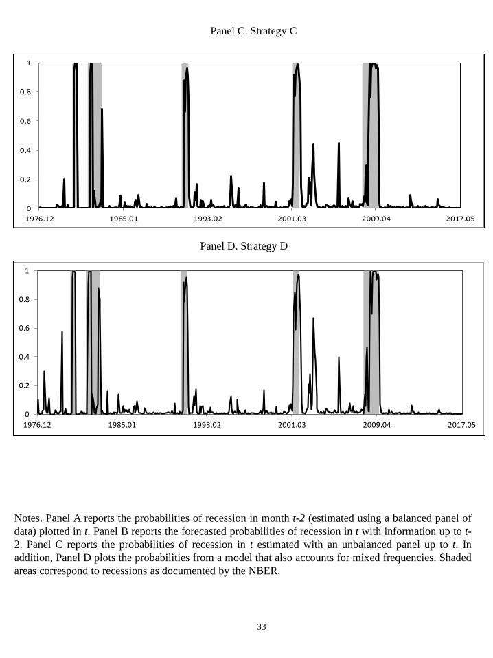
Strategies A and B clearly miss the extremely valuable information about the current

business cycle that is provided by the early published indicators. In particular, these infer-

ences miss the data of personal income at t�1, and industrial production and employment

at t � 1 and t. To overcome this drawback, the business cycle inferences are computed

in strategy C by using the extension of MS-DFM proposed in this paper to deal with

ragged-edge data. Finally, the inferences are also computed in strategy D by enlarging

this model with GDP, which requires dealing with mixed frequencies described in Section

2.

Figure 2, which plots the real-time �ltered probabilities estimated from strategies A

(panel A), B (panel B), C (panel C), and D (panel D), respectively, helps us to assess

the empirical performance of the di¤erent strategies in real time. As expected, when the

analysis is developed in real time the �gures show a signi�cant deterioration in the mod-

els�performance with respect to the in-sample results. Although the in-sample �ltered

probabilities plotted in Figure 1, which are computed from �nally revised data, provide

unequivocal jumps in probabilities that marked the start and the end of the US busi-

ness cycle phases, the real-time probabilities plotted in Figure 2 produce noisier and less

accurate signals of the business cycle.

The �gures also show that there is a signi�cant improvement in business cycle fore-

casting accuracy when the MS-DFM is allowed to deal with ragged-edge data. To evaluate

these forecasting improvements, Table 3 displays the results of the real-time FQPS for the

four di¤erent strategies. According to our theoretical and Monte Carlo results, strategy

C provides much better forecasting accuracy than strategies A and B, with a reduction in

FQPS of more than 35%. To analyze whether empirical loss di¤erences across the com-

peting models and Strategy C are statistically signi�cant, the last row of the table shows in

brackets the p-values of the pairwise test introduced by Diebold and Mariano (DM, 1995),

which is the most in�uential test in the literature of equal forecasting accuracy. According

to the p-values of the DM test, the reductions in FQPS achieved with the model that

manage ragged-ends data are statistically signi�cant at standard signi�cance levels.

20

Notably, the MS-DFM that additionally accounts for mixed frequencies does not seem

to exhibit signi�cant reductions in FQPS to that achieved by the MS-DFM that uses the

unbalanced panel of only four monthly indicators (FQPS of 0.055 and 0.052, respectively).

In addition, the equal predictive accuracy tests show that the di¤erences in forecasting

accuracy between Strategy C and Strategy D are not statistically signi�cant. Therefore,

our empirical application shows that, although using early available information from the

set of four monthly indicators substantially improves the US business cycle inferences

in real time, adding the information provided by quarterly GDP does not appear to be

relevant.

6 Concluding remarks

Real-time data usually display the feature of ragged ends, which means that end-of-sample

observations of time series are missing and only released with a time-lag. The asynchro-

nous publication releases limit the empirical bene�ts of Markov-switching dynamic factor

models in monitoring the day-to-day economic developments because these models are

restricted to dealing with balanced data vintages and cannot manage all the relevant new

releases as they arrive. In practice, the business cycle inferences computed from these

models are either available only with a delay of several months or they are computed as

forecasts of past inferences.

From the point of view of monitoring business cycle conditions, we show in the paper

that there is no reason to be late or to disregard the relevant information provided by the

latest �gures of promptly issued indicators. We theoretically show that, when the economic

indicators are carefully selected to have large signal-to-noise ratios in the Kalman �lter

used to compute business cycle inferences, the increase in the accuracy of business cycle

identi�cation becomes substantial.

The extension of dynamic factor models with regime switches proposed in this paper is

the missing piece of this puzzle. Following the linear proposal of Mariano and Murasawa

(2003), the method is based on a nonlinear Kalman �lter to �ll in the gaps of the non-

synchronous �ow of data releases in an e¢ cient manner. By means of several Monte Carlo

21

experiments, we quantify the magnitude of the accuracy improvements provided by our

proposal over traditional methods, which substantially depends on the signal-to-noise ratio

of the early available indicators.

In addition, traditional Markov-switching dynamic factor models cannot deal with

business cycle indicators of di¤erent -typically monthly and quarterly- frequencies. In this

paper, we also show how to mix monthly and quarterly indicators to infer the business cy-

cle phases. The method treat quarterly data as monthly data that exhibit missing monthly

observations within each quarter. Accordingly, the nonlinear state-space framework pro-

posed to deal with ragged-edge data can also be used to combine business cycle indicators

of di¤erent frequencies.

In the empirical application considered in this paper, we �nd that our theoretical �nd-

ings are borne out. We use a real-time collection of data vintages which are updated

monthly using only the information that would have been available at each month over

the last four decades. The vintages use the four constituent monthly series of the Stock-

Watson coincident index. Our extension produces real-time business cycle probabilities

that track the business cycle accurately, with pronounced drops corresponding to the

NBER-designated recessions. Notably, we obtain substantial improvements in our exten-

sion of Markov-switching dynamic factor models with respect to forecasting the probabili-

ties from balanced panels of indicators. However, we failed to �nd signi�cant improvements

when GDP is used as an additional indicator.

One potential limitation of the model is that it does not take into account revisions to

the indicator initial releases, which are known to be sometimes quite large. The inaccu-

racy of initial data complicates decision making by policymakers and other agents whose

optimal choices depend on the state of the economy. We consider that this extension is

important enough to leave it for further research.

22

AppendixProof of Proposition 1: To evaluate the information content of yk;t+1jt , note that

f(yk;t+1jtjst+1 = i; It) =1�p

2��k ����(i)k;t+1jt���1=2 exp(�

1

2(yk;t+1��kf (i)t+1jt)

0��(i)k;t+1jt

��1(yk;t+1��kf (i)t+1jt))

(A1)

for i = 0; 1where�(i)k;t+1jt is the variance of yk;tjst+1 = i; It, which for brevity we will denote

�i and f(i)t+1jt = E(f t+1jst+1 = i; It) denoted more brie�y as f i: Using the notation in

Cover and Thomas (2006) for the multiple integral, then

KL =

Zlnf(yk;t+1jst+1 = 1; It)f(yk;t+1jst+1 = 0; It)

f(yk;t+1jst = 1; It)dyk;t+1

=

Z� ln(f(yk;t+1jst+1 = 0; It))f(yk;t+1jst = 1; It)dyk;t+1

�Z� ln(f(yk;t+1jst+1 = 1; It))f(yk;t+1jst = 1; It)dyk;t+1

= K0 �K1;

where Ki is the entropy of f(yk;t+1jst+1 = i; It), i = 0; 1 with respect to the conditional

density f(yk;t+1jst = 1; It). The entropy of a Gaussian distribution is given by (see, for

instance, Cover and Thomas, 2006)

K1 =1

2ln(2�)k j�1j+

k

2:

The �rst part of the integral K0 is given by

K0 =

Z� ln(f(yk;t+1jst+1 = 0; It))f(yk;t+1jst = 1; It)dyk;t+1

=1

2

Z(yk;t+1 ��kf0)0��10 (yk;t+1 ��kf0)f(yk;t+1jst = 1; It)dyk;t+1

+1

2

Zln(2�)k j�0j f(yk;t+1jst = 1; It)dyk;t+1

Summing and subtracting �kf1 so the expectation in the previous expression does not

23

change, the previous integral can be written as

K0 =

Z� ln(f(yk;t+1jst+1 = 0; It))f(yk;t+1jst = 1; It)dyk;t+1

=1

2

Z(yk;t+1 ��kf1 ��kf0 +�kf1)0��10 (yk;t+1 ��kf1 ��kf0 +�kf1)f(yk;t+1jst = 1; It)dyk;t+1

+1

2ln(2�)k j�0j

=1

2

Z(yk;t+1 ��kf1)0��10 (yk;t+1 ��kf1)f(yk;t+1jst = 1; It)dyk;t+1

+1

2

Z(f1 � f0)0�0k��10 �k(f1 � f0)f(yk;t+1jst = 1; It)dyk;t+1

�Z(yk;t+1 ��kf1)0��10 �k(f1 � f0)f(yk;t+1jst = 1; It)dyk;t+1

+1

2ln(2�)k j�0j

=1

2�1�

�10 + (f1 � f0)0�0k��10 �k(f1 � f0) +

1

2ln(2�)k j�0j

where to obtain the result we have taken into account that E(yk;t+1jst+1 = 1; It) = �kf1.

Then, The Kullback Leibler divergence is given by

KL = K0 �K1

=1

2�1�

�10 + (f1 � f0)0�0k��10 �k(f1 � f0) +

1

2ln(2�)k(j�0j � j�1j)�

k

2;

which is the desired expression.

24

Proof of Corollary: In this case

f(yk;t+1jtjst+1 = i; It) =1�p

2��k ���k;t+1jt��1=2 exp(�

1

2(yk;t+1��kf (i)t+1jt)

0��1k;t+1jt(yk;t+1��kf(i)t+1jt))

(A1)

for i = 0; 1where �k;t+1jt is the variance of yk;tjst+1 = i; It, which we have assumed to

be the same in both states and f (i)t+1jt = E(ft+1jst+1 = i; It): Then, the Kullback-Leibler

divergence is now given by (??) for the case r = 1;

KL =1

2

�f(0)t+1jt � f

(1)t+1jt

�2�0k�

�1k;t+1jt�k

=1

2(�0 � �1)2�0k��1k;t+1jt�k: (A2)

Let �k;u = didag(�21; :::; �2k) be the idiosyncratic variance of the k promptly issued indica-

tors yk;t+1. Taking into account the expression for the inverse of the sum of two matrices

(see, for instance, Rao, 1973)

��1k;t+1jt = ��1k;u ��

�1k;u�k

�P�1t+1jt +�

0k�

�1k;u�k

��1�0k�

�1k;u: (A3)

where Pt+1jt = E�ft+1 � ft+1jtjIt

�2 is given byPt+1jt = �2Ptjt + �

2a: (A4)

Plugging (A3) and (A4) into (A2)

KL =1

2(�0 � �1)2

0B@ kXi=1

�2i�2i�

�Pki=1

�2i�2i

�2Pki=1

�2i�2i+ 1

�2Ptjt+�2a

1CA=

1

2(�0 � �1)2

1�2Ptjt+�2a

Pki=1

�2i�2iPk

i=1�2i�2i+ 1

�2Ptjt+�2a

=1

2(�0 � �1)2

0@ 1Pki=1

�2i�2i

+ �2Ptjt + �2a

1A�1

(A5)

which is the desired expression.

25

References

[1] Aruoba, B., Diebold, F., and Scotti, C. 2009. Real-time measurement of business

conditions. Journal of Business and Economic Statistics 27: 417-427.

[2] Barhoumi, K, Darne O. and Ferrara, L. Dynamic Factor Models: A review of the

literature. 2014. Journal of Business Cycle Measurement and Analysis, Number 8,

Issue 2

[3] Berje, T, and Jorda, O. 2011. The classi�cation of economic activity into expansions

and recessions. American Economic Journal: Macroeconomics 3: 246-277

[4] Burns, A., and Mitchell, W. 1946. Measuring business cycles. National Bureau of

Economic Research, New York.

[5] Camacho, M., and Perez Quiros, G., and Poncela, P. 2015. Extracting nonlinear

signals from several economic indicators. Journal of Applied Econometrics 30: 1073-

1089.

[6] Camacho, M., and Perez Quiros, G. 2007. Jump-and-rest e¤ect of U.S. business cycles.

Studies in Nonlinear Dynamics and Econometrics 11(4): article 3.

[7] Chauvet, M. 1998. An econometric characterization of business cycle dynamics with

factor structure and regime switches. International Economic Review 39: 969-96.

[8] Chauvet, M., and Hamilton, J. 2006. Dating business cycle turning points in real time.

In Nonlinear Time Series Analysis of Business Cycles, eds. C. Milas, P. Rothman,

and D. Van Dijk. Amsterdam: Elsevier Science, pp. 1-54.

[9] Chauvet, M., and Piger, J. 2008. A comparison of the real-time performance of busi-

ness cycle dating methods. Journal of Business and Economic Statistics 26: 42-49.

[10] Cover, T. and Thomas, J. 2006. Elements of information theory.Wiley, New Jersey.

[11] Cui, S. 2016. Comparison of approximation methods to Kullback-Leibler divergence

between Gaussian mixture models for satellite image retrieval. Remote Sensing Letters

7(7): 651-660.

26

[12] Diebold, F., and Rudebusch, G. 1991. Forecasting output with the composite leading

index: A real-time analysis. Journal of the American Statistical Association 86: 603-

610.

[13] Diebold, F., and Rudebusch, G. 1996. Measuring business cycles: A modern perspec-

tive. Review of Economics and Statistics 78: 67-77.

[14] Evans M. 2005. Where are we now? Real time estimates of the macroeconomy. In-

ternational Journal of Central Banking 1: 127-175.

[15] Hamilton, J. 1989. A new approach to the economic analysis of nonstationary time

series and the business cycles. Econometrica 57: 357-384.

[16] Hamilton, J. 2011. Calling recessions in real time. International Journal of Forecasting

27: 1006-1026.

[17] Kim, C. 1994. Dynamic linear models with Markov-switching. Journal of Economet-

rics 60: 1-22.

[18] Kim, C., and Nelson, C. 1998. Business cycle turning points, a new coincident in-

dex, and tests of duration dependence based on a dynamic factor model with regime

switching. Review of Economics and Statistics 80: 188-201.

[19] Kim, C., and Yoo, J.S. 1995. New index of coincident indicators: A multivariate

Markov switching factor model approach. Journal of Monetary Economics 36: 607-

630.

[20] Lam, C., Yao, Q., and Bathia, N. 2011. Estimation of latent factors using high-

dimensional time series. Biometrika, 98(4):901-918.

[21] Mariano, R., and Murasawa, Y. 2003. A new coincident index os business cycles based

on monthly and quarterly series. Journal of Applied Econometrics 18: 427-443.

[22] Michalowicz, J.V., Nichols, J.M. and Bucholtz, F. 2008. Calculation of di¤erential

entropy for a mixed Gaussian distribution. Entropy 10: 200-206.

27

[23] Poncela, P. and Ruiz, E. 2015. More is not always better: back to the Kalman �lter in

Dynamic Factor Models in Unobserved Components and Time Series Econometrics

(Koopman and Shephard, Eds), chapter 11. Oxford University Press.

[24] Proietti, T. and Moauro, F. 2006. Dynamic factor analysis with non-linear temporal

aggregation constraints. Appl. Statist. 55: 281-300.

[25] Rao, C. R. 1973. Linear Statistical Inference and Its Applications. New York: J.

Wiley.

[26] Stock, J., and Watson, M. 1991. A probability model of the coincident economic in-

dicators. In Leading Economic Indicators: New Approaches and Forecasting Records,

edited by K. Lahiri and G. Moore, Cambridge University Press.

28

29

Table 1. Analysis of ragged ends in MS-DFM

Balanced panels Unbalanced panels

2

=0.3 =0.6 =0.3 =0.6

N=5 N=7 N=5 N=7 N=1+4 N=3+4 N=1+4 N=3+4

µ0=

1,

µ1=

-1 0.5

0.062

(0.086)

0.060

(0.085)

0.069

(0.089)

0.061

(0.087)

0.047

(0.051)

0.043

(0.046)

0.055

(0.062)

0.048

(0.051)

1.5 0.069

(0.089)

0.066

(0.088)

0.079

(0.094)

0.069

(0.092)

0.055

(0.062)

0.053

(0.056)

0.063

(0.071)

0.055

(0.061)

4.5 0.077

(0.099)

0.076

(0.098)

0.104

(0.109)

0.085

(0.106)

0.070

(0.085)

0.068

(0.079)

0.084

(0.088)

0.072

(0.073)

2

=0.3 =0.6 =0.3 =0.6

N=5 N=7 N=5 N=7 N=1+4 N=3+4 N=1+4 N=3+4

µ0=

2,

µ1=

-1 0.5

0.047

(0.073)

0.041

(0.072)

0.048

(0.074)

0.042

(0.073)

0.028

(0.031)

0.018

(0.022)

0.031

(0.035)

0.020

(0.028)

1.5 0.048

(0.075)

0.043

(0.073)

0.052

(0.078)

0.045

(0.070)

0.031

(0.035)

0.021

(0.028)

0.035

(0.041)

0.024

(0.031)

4.5 0.064

(0.082)

0.053

(0.080)

0.079

(0.092)

0.062

(0.088)

0.042

(0.050)

0.026

(0.035)

0.054

(0.061)

0.038

(0.048)

Notes. N is the number of indicators and 2 is the variance of their idiosyncratic

components. In balanced MS-DFM, entries show the average over the replications of the

squared deviation of one- and two- (in brackets) step-ahead filtered probabilities of low-

mean state from the 1000 generated business cycle sequences. In MS-DFM with

unbalanced panels, 1 and 3 variables with variance 1.5 are assumed to be timely available

when the inference is computed and 4 indicators with variance 0.5, 1.5 and 4.5 are

published with one- and two-month lags. High-growth and low-growth means are µ0 and

µ1, respectively; is the autoregressive parameter of the idiosyncratic components.

30

Table 3. Maximum likelihood estimates

Monthly

IP Empl Inc Sales

Indicators

i

0.69

(0.03)

0.42

(0.02)

0.28

(0.04)

0.46

(0.03)

1

-0.18

(0.08)

0.24

(0.03)

-0.20

(0.02)

-0.34

(0.04)

2 -0.16

(0.08)

0.54

(0.04)

-0.05

(0.04)

-0.15

(0.05)

2

i 0.26

(0.04)

0.27

(0.02)

0.85

(0.03)

0.57

(0.03)

Factor 0 1

2*a

p00 p11

0.32

(0.07)

-2.00

(0.20) 1

0.98

(0.01)

0.85

(0.05)

Monthly and quarterly

IP Empl Inc Sales GDP

Indicators

i

0.67

(0.03)

0.42

(0.02)

0.29

(0.04)

0.48

(0.03)

0.30

(0.02)

1

-0.07

(0.07)

0.24

(0.03)

-0.21

(0.02)

-0.37

(0.04)

0.024

(0.40)

2 -0.07

(0.07)

0.54

(0.04)

-0.06

(0.04)

-0.17

(0.05)

-0.57

(0.22)

2

i 0.55

(0.04)

0.51

(0.02)

0.91

(0.03)

0.73

(0.03)

0.47

(0.15)

Factor 0 1

2*a

p00 p11

0.29

(0.07)

-2.00

(0.21) 1

0.98

(0.01)

0.83

(0.06)

Notes. Standard errors are in parentheses

Table 3. Real-time (1976.10-2017.05) empirical performance

Strategy A Strategy B Strategy C Strategy D

Balanced Balanced Unbalanced Unbalanced

Mixed frequency

0.086

(0.005)

0.083

(0.006)

0.055

(-)

0.052

(0.321)

Note. Entries refer to FQPS statistics. The figures within parentheses show the p-values of

the Diebold-Mariano (DM) test of equal forecast accuracy between Strategy C and the rest

of strategies. The forecasting strategies are defined in the text.

31

Note. These graph plots the common factor (left scale) and the smoothed probabilities of recession

(right scale). Panel A refers to refers to the model of four monthly indicators while Panel B refers to the

model that adds GDP. Shaded areas correspond to recessions as documented by the NBER.

Figure 1. In-sample results 1967.04-2017.03

0

0.2

0.4

0.6

0.8

1

-7

-3.5

0

3.5

1967.04 1974.05 1981.06 1988.07 1995.08 2002.09 2009.1 2016.11

0

0.2

0.4

0.6

0.8

1

-7

-3.5

0

3.5

1967.04 1974.05 1981.06 1988.07 1995.08 2002.09 2009.1 2016.11

Panel A. Four monthly indicators

Panel B. Four monthly indicators and quarterly GDP

32

Figure 2. Real time probabilities 1976.12-2017.05

0

0.2

0.4

0.6

0.8

1

1976.12 1985.01 1993.02 2001.03 2009.04 2017.05

Panel A. Strategy A

Panel B. Strategy B

0

0.2

0.4

0.6

0.8

1

1976.12 1985.01 1993.02 2001.03 2009.04 2017.05

33

Notes. Panel A reports the probabilities of recession in month t-2 (estimated using a balanced panel of

data) plotted in t. Panel B reports the forecasted probabilities of recession in t with information up to t-

2. Panel C reports the probabilities of recession in t estimated with an unbalanced panel up to t. In

addition, Panel D plots the probabilities from a model that also accounts for mixed frequencies. Shaded

areas correspond to recessions as documented by the NBER.

0

0.2

0.4

0.6

0.8

1

1976.12 1985.01 1993.02 2001.03 2009.04 2017.05

Panel C. Strategy C

Panel D. Strategy D

0

0.2

0.4

0.6

0.8

1

1976.12 1985.01 1993.02 2001.03 2009.04 2017.05