1162 IEEE TRANSACTIONS ON INTELLIGENT TRANSPORTATION SYSTEMS, VOL. 16, NO. 3, JUNE 2015
Fully Automatic Roadside Camera Calibrationfor Traffic Surveillance
Markéta Dubská, Adam Herout, Roman Juránek, and Jakub Sochor
Abstract—This paper deals with automatic calibration of road-side surveillance cameras. We focus on parameters necessary formeasurements in traffic-surveillance applications. Contrary to theexisting solutions, our approach requires no a priori knowledge,and it works with a very wide variety of road settings (numberof lanes, occlusion, quality of ground marking), as well as withpractically unlimited viewing angles. The main contribution isthat our solution works fully automatically—without any per-camera or per-video manual settings or input whatsoever—andit is computationally inexpensive. Our approach uses tracking oflocal feature points and analyzes the trajectories in a mannerbased on cascaded Hough transform and parallel coordinates. Animportant assumption for the vehicle movement is that at least apart of the vehicle motion is approximately straight—we discussthe impact of this assumption on the applicability of our approachand show experimentally that this assumption does not limit theusability of our approach severely. We efficiently and robustlydetect vanishing points, which define the ground plane and vehiclemovement, except for the scene scale. Our algorithm also computesparameters for radial distortion compensation. Experiments showthat the obtained camera parameters allow for measurements ofrelative lengths (and potentially speed) with ∼2% mean accuracy.The processing is performed easily in real time, and typically, a2-min-long video is sufficient for stable calibration.
Index Terms—Camera calibration, camera distortion correc-tion, camera surveillance, diamond space, ground plane esti-mation, Hough transform, orthogonal vanishing points, PClines,speed estimation, vanishing points (VPs).
I. INTRODUCTION
THE number of Internet-connected cameras is quickly in-creasing, and a notable amount of them are used in traffic
monitoring. At the moment, many of these are used primarilyfor simply transferring the image to a human operator, and theylack automatic processing. This is mainly because machine-vision-based data mining algorithms require manual configura-tion and maintenance, involving a considerable effort of skilledpersonnel and, in many cases, measurements and actions takenin the actual real-life scene [1]–[6]. The goal of our research isto provide fully automatic (no manual input whatsoever) traffic
Manuscript received January 28, 2014; revised June 11, 2014; acceptedAugust 19, 2014. Date of publication September 24, 2014; date of current versionMay 29, 2015. This work was supported by TACR project V3C, TE01020415,and by the IT4Innovations Centre of Excellence, ED1.1.00/02.0070. The Asso-ciate Editor for this paper was K. Wang.
M. Dubská, R. Juránek, and J. Sochor are with the Graph@FIT, BrnoUniversity of Technology, 612 66 Brno, Czech Republic.
A. Herout is with the Graph@FIT, Brno University of Technology, 612 66Brno, Czech Republic, and also with Angelcam, Inc., Minden, NV 89423-8607USA.
Color versions of one or more of the figures in this paper are available onlineat http://ieeexplore.ieee.org.
Digital Object Identifier 10.1109/TITS.2014.2352854
processing algorithms—leading toward vehicle classificationand counting, speed measurement, congestion detection, etc.Different applications can be fostered by compensation of localprojection [7].
In this paper, we are dealing with the problem of fullyautomatic camera calibration in a common traffic-monitoringscenario. We automatically determine radial distortion compen-sation parameters and solve the calibration of internal cameraparameters and external parameters (camera orientation andposition up to scale with respect to the dominant motion of thevehicles). The solution is fully automatic in the sense that thereare no inputs or configuration parameters specific to a particulartraffic setting, camera type, etc. In addition, we are not assum-ing any appearance model of the vehicles, which would differfor different countries, time periods, and the kind of traffic onthe particular road. Moreover, we assume no a priori knowl-edge about the road itself (number of lanes, appearance of themarking, presence of specific features, etc.). The only assump-tion is approximately straight shape of the road. Experimentsshow that normal curves on highways are still “straight enough”to meet our assumption. Sharp corners cannot be directly han-dled by our approach and will be subject of further study.
Because of the lack of information that can be obtained fromroad data, the majority of methods assume the principal pointto be at the center of the image [8], [9]. A popular assumptionalso is a horizontal horizon line, i.e., zero roll of the camera[8], [10], [11]—which turns out to be severely limiting, becauseit is difficult to find an actual roadside camera meeting thisassumption accurately enough.
Some works require user input in the form of annotation ofthe lane marking with known lane width [2], [6] or markingdimensions [3], camera position [2], [12], and average vehiclesize [13] or average vehicle speed [8]. A common feature ofvirtually all methods is detection of the vanishing point (VP)corresponding to the direction of moving vehicles. A popularapproach to obtaining this VP is to use road lines [5], [9], [14]or lanes [9], [11], more or less automatically extracted from theimage. These approaches typically require a high number oftraffic lanes and a consistent and well-visible lane marking.
Another class of methods disregards the line marking onthe road (because of its instability and impossible automaticdetection) and observes the motion of the vehicles, assumingstraight and parallel trajectories in a dominant part of the view.Schoepflin and Dailey [8] constructed an activity map of theroad with multiple lanes and segmented out individual lanes.Again, this approach relies on observing a high number of traf-fic lanes—high-capacity motorways and similar settings. Otherresearchers detect vehicles by a boosted detector and observe
DUBSKÁ et al.: FULLY AUTOMATIC ROADSIDE CAMERA CALIBRATION FOR TRAFFIC SURVEILLANCE 1163
their movement [15] or analyze edges present on the vehicles[16]. Beymer et al. [4] accumulated tracked feature points,but also required the user to provide defined lines by manualinput. Kanhere and Birchfield [17] took a specific approach forcameras placed low above the street level. Once the calibrationand scene scale is available, the road plane can be rectified, andvarious applications such as speed measurement can be done ina straightforward manner [3], [6], [10], [12], [18].
We assume that the shape of the road is (approximately)straight, and therefore, the majority of vehicles move in straightmutually parallel trajectories. Our experiments verify that ourapproach is tolerant to a high rate of outliers from this assump-tion. We are using a variant of the Hough transform, which isvery tolerant to random outliers, and these do not affect thefound global maximum. Due to this, vehicles changing lanes,passing one another, or avoiding a small obstacle do not harmthe algorithm, and our method is easily and reliably applicableon a vast majority of real traffic-surveillance videos (of approx-imately straight roads). The calibration of internal and externalparameters of the camera is achieved by first computing threeorthogonal VPs [19]–[21], which define the vehicle motion.
Our calibration is provided up to scale, which is generallyimpossible to determine (from just an image, one can nevertell a matchbox model from real vehicles). The scale can beprovided manually [2], [12] or recognized by detecting knownobjects [13].
We harness our finite and linear parameterization of the realprojective plane published recently [22]. In this previous work,we streamlined the cascaded Hough Transform by stacking twostages and skipping one intermediate accumulation step. Thisapproach allows for detection of VPs (and triplets of orthogonalVPs) from noisy linelet data. These input data can be com-ing online and be accumulated to a fixed-size accumulationspace—which is suitable in online video processing. Insteadof using road marking or lane border edges [3], [5], [8], weaccumulate fractions of trajectories of detected feature pointson moving objects and relevant edges.
Contrary to previous works, our approach provides the cam-era calibration fully automatically for very versatile cameraviews and road contexts (coming and going vehicles, fromthe side, from the top, small roads and highways, close-upand fisheye lenses, and so on). The method can be appliedon virtually any roadside camera without any user input—theexperiments presented in this paper were done without any per-camera or per-video settings.
We collected a set of video recordings of traffic on roadsof different scales, with various cameras, in different weatherconditions. The MATLAB source codes and the video data setare publicly available for comparison and future work.1
II. AUTOMATIC ROADSIDE CAMERA CALIBRATION
Let us consider a road scene with a single principal directionof the vehicle movement. The position of the ground plane andthe direction of the vehicle movement relative to the camera canbe defined and described by three VPs [19], [20].
1http://medusa.fit.vutbr.cz/pclines
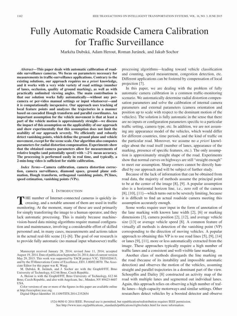
Fig. 1. We propose a fully automatic approach to camera calibration byrecognizing the three dominant VPs, which characterize the vehicles and theirmotion. (Top) Three recognized VPs. (Bottom) Various scenes in which thealgorithm automatically calibrates the camera.
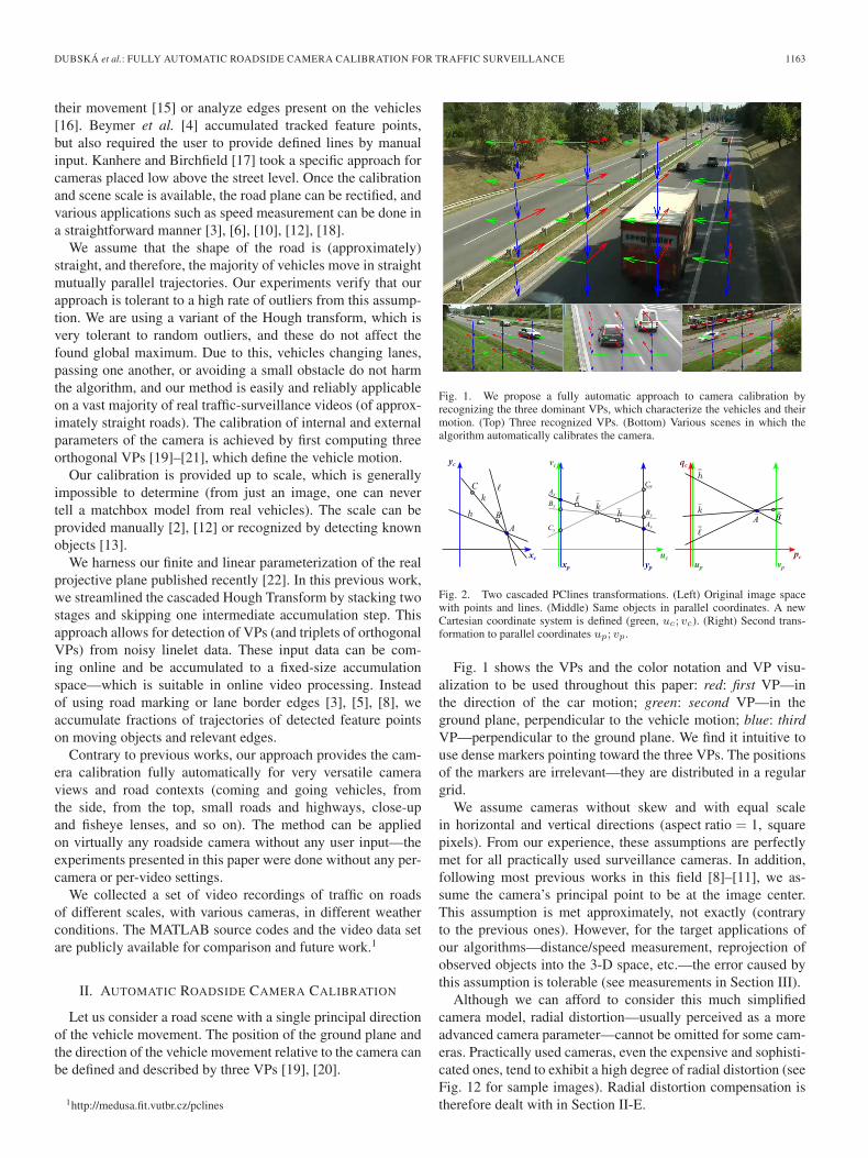
Fig. 2. Two cascaded PClines transformations. (Left) Original image spacewith points and lines. (Middle) Same objects in parallel coordinates. A newCartesian coordinate system is defined (green, uc; vc). (Right) Second trans-formation to parallel coordinates up; vp.
Fig. 1 shows the VPs and the color notation and VP visu-alization to be used throughout this paper: red: first VP—inthe direction of the car motion; green: second VP—in theground plane, perpendicular to the vehicle motion; blue: thirdVP—perpendicular to the ground plane. We find it intuitive touse dense markers pointing toward the three VPs. The positionsof the markers are irrelevant—they are distributed in a regulargrid.
We assume cameras without skew and with equal scalein horizontal and vertical directions (aspect ratio = 1, squarepixels). From our experience, these assumptions are perfectlymet for all practically used surveillance cameras. In addition,following most previous works in this field [8]–[11], we as-sume the camera’s principal point to be at the image center.This assumption is met approximately, not exactly (contraryto the previous ones). However, for the target applications ofour algorithms—distance/speed measurement, reprojection ofobserved objects into the 3-D space, etc.—the error caused bythis assumption is tolerable (see measurements in Section III).
Although we can afford to consider this much simplifiedcamera model, radial distortion—usually perceived as a moreadvanced camera parameter—cannot be omitted for some cam-eras. Practically used cameras, even the expensive and sophisti-cated ones, tend to exhibit a high degree of radial distortion (seeFig. 12 for sample images). Radial distortion compensation istherefore dealt with in Section II-E.
1164 IEEE TRANSACTIONS ON INTELLIGENT TRANSPORTATION SYSTEMS, VOL. 16, NO. 3, JUNE 2015
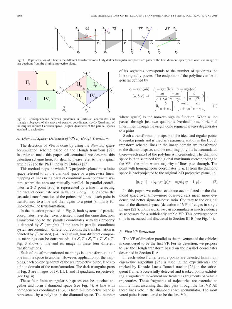
Fig. 3. Representation of a line in the different transformations. Only darker triangular subspaces are parts of the final diamond space; each one is an image ofone quadrant from the original projective plane.
Fig. 4. Correspondence between quadrants in Cartesian coordinates andtriangle subspaces of the space of parallel coordinates. (Left) Quadrants ofthe original infinite Cartesian space. (Right) Quadrants of the parallel spacesattached to each other.
A. Diamond Space: Detection of VPs by Hough Transform
The detection of VPs is done by using the diamond spaceaccumulation scheme based on the Hough transform [22].In order to make this paper self-contained, we describe thisdetection scheme here; for details, please refer to the originalarticle [22] or the Ph.D. thesis by Dubská [23].
This method maps the whole 2-D projective plane into a finitespace referred to as the diamond space by a piecewise linearmapping of lines using parallel coordinates—a coordinate sys-tem, where the axes are mutually parallel. In parallel coordi-nates, a 2-D point [x, y] is represented by a line intersectingthe parallel coordinate axis in values x or y. Fig. 2 shows thecascaded transformation of the points and lines—each point istransformed to a line and then again to a point (similarly forline–point–line transformation).
In the situation presented in Fig. 2, both systems of parallelcoordinates have their axes oriented toward the same direction.Transformation to the parallel coordinates with this propertyis denoted by S (straight). If the axes in parallel coordinatesystem are oriented in different directions, the transformation isdenoted by T (twisted) [24]. As a result, four different compos-ite mappings can be constructed: S ◦ S, T ◦ S, T ◦ T ,S ◦ T .Fig. 3 shows a line and its image in these four differenttransformations.
Each of the aforementioned mappings is a transformation ofone infinite space to another. However, application of the map-pings, each on one quadrant of the real projective plane, leads toa finite domain of the transformation. The dark triangular partsin Fig. 3 are images of IV, III, I, and II quadrant, respectively(see Fig. 4).
These four finite triangular subspaces can be attached to-gether and form a diamond space (see Fig. 4). A line withhomogeneous coordinates (a, b, c) from 2-D projective plane isrepresented by a polyline in the diamond space. The number
of its segments corresponds to the number of quadrants theline originally passes. The endpoints of the polyline can be ingeneral defined by
α = sgn(ab) β = sgn(bc) γ = sgn(ac)
(a, b, c) →[
αa
c+ γa,
−αc
c+ γa
],
[b
c+ βb, 0
],[
0,b
a+ αb
],
[−αa
c+ γa,
αc
c+ γa
](1)
where sgn(x) is the nonzero signum function. When a linepasses through just two quadrants (vertical lines, horizontallines, lines through the origin), one segment always degeneratesto a point.
Such a transformation maps both the ideal and regular pointsto regular points and is used as a parameterization in the Houghtransform scheme: lines in the image domain are transformedto the diamond space, and the resulting polyline is accumulatedthere—each pixel of the polyline is incremented. The diamondspace is then searched for a global maximum corresponding tothe VP—the point where majority of lines pass through. Thepoint with homogeneous coordinates [p, q, 1] from the diamondspace is backprojected to the original 2-D projective plane, i.e.,
[p, q, 1] → [q, sgn(p)p+ sgn(q)q − 1, p] . (2)
In this paper, we collect evidence accumulated to the dia-mond space over time—more observed cars mean more evi-dence and better signal-to-noise ratio. Contrary to the originaluse of the diamond space (detection of VPs of edges in singleimages [22]), in this work, we can accumulate as much evidenceas necessary for a sufficiently stable VP. This convergence intime is measured and discussed in Section III-B (see Fig. 14).
B. First VP Extraction
The VP of direction parallel to the movement of the vehiclesis considered to be the first VP. For its detection, we proposeto use the Hough transform based on the parallel coordinatesdescribed in Section II-A.
In each video frame, feature points are detected (minimumeigenvalue algorithm [25] is used in the experiments) andtracked by Kanade–Lucas–Tomasi tracker [26] in the subse-quent frame. Successfully detected and tracked points exhibit-ing a significant movement are treated as fragments of vehicletrajectories. These fragments of trajectories are extended toinfinite lines, assuming that they pass through the first VP. Allthese lines vote in the diamond space accumulator. The mostvoted point is considered to be the first VP.
DUBSKÁ et al.: FULLY AUTOMATIC ROADSIDE CAMERA CALIBRATION FOR TRAFFIC SURVEILLANCE 1165
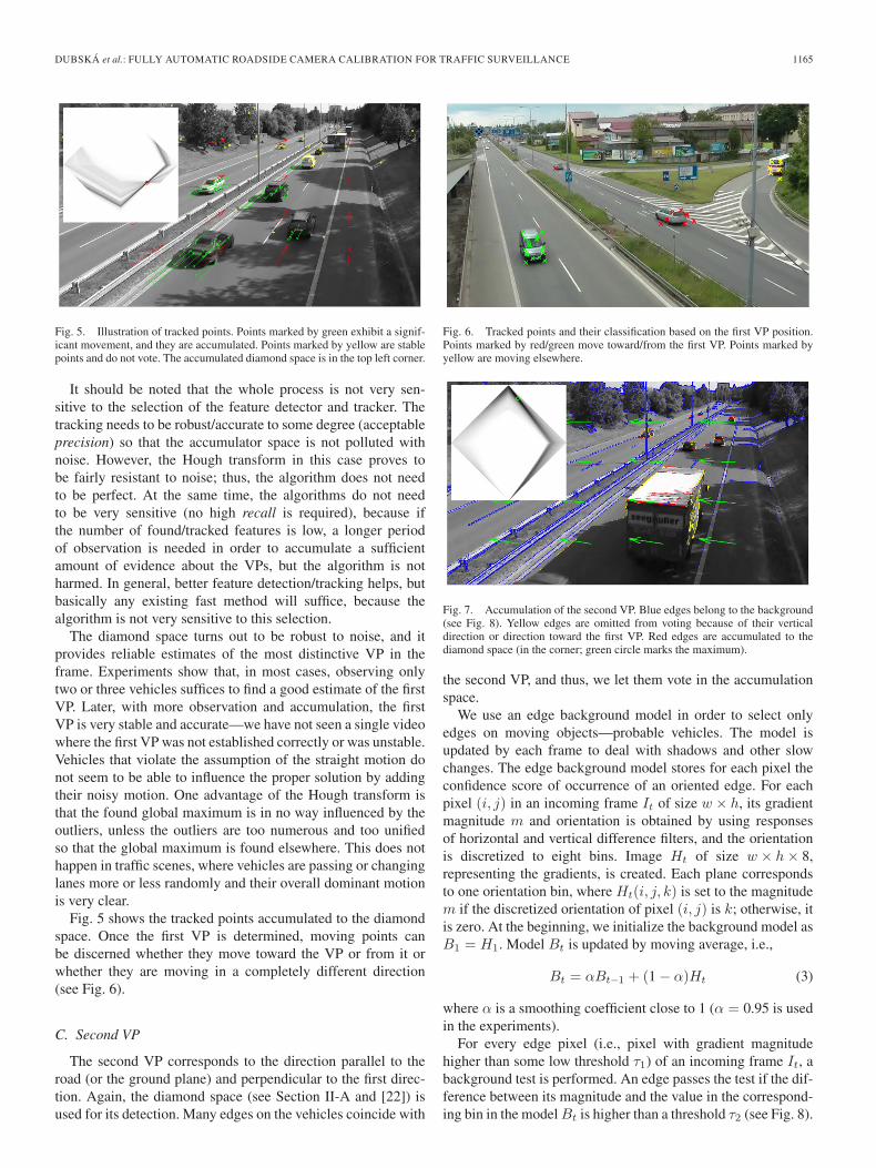
Fig. 5. Illustration of tracked points. Points marked by green exhibit a signif-icant movement, and they are accumulated. Points marked by yellow are stablepoints and do not vote. The accumulated diamond space is in the top left corner.
It should be noted that the whole process is not very sen-sitive to the selection of the feature detector and tracker. Thetracking needs to be robust/accurate to some degree (acceptableprecision) so that the accumulator space is not polluted withnoise. However, the Hough transform in this case proves tobe fairly resistant to noise; thus, the algorithm does not needto be perfect. At the same time, the algorithms do not needto be very sensitive (no high recall is required), because ifthe number of found/tracked features is low, a longer periodof observation is needed in order to accumulate a sufficientamount of evidence about the VPs, but the algorithm is notharmed. In general, better feature detection/tracking helps, butbasically any existing fast method will suffice, because thealgorithm is not very sensitive to this selection.
The diamond space turns out to be robust to noise, and itprovides reliable estimates of the most distinctive VP in theframe. Experiments show that, in most cases, observing onlytwo or three vehicles suffices to find a good estimate of the firstVP. Later, with more observation and accumulation, the firstVP is very stable and accurate—we have not seen a single videowhere the first VP was not established correctly or was unstable.Vehicles that violate the assumption of the straight motion donot seem to be able to influence the proper solution by addingtheir noisy motion. One advantage of the Hough transform isthat the found global maximum is in no way influenced by theoutliers, unless the outliers are too numerous and too unifiedso that the global maximum is found elsewhere. This does nothappen in traffic scenes, where vehicles are passing or changinglanes more or less randomly and their overall dominant motionis very clear.
Fig. 5 shows the tracked points accumulated to the diamondspace. Once the first VP is determined, moving points canbe discerned whether they move toward the VP or from it orwhether they are moving in a completely different direction(see Fig. 6).
C. Second VP
The second VP corresponds to the direction parallel to theroad (or the ground plane) and perpendicular to the first direc-tion. Again, the diamond space (see Section II-A and [22]) isused for its detection. Many edges on the vehicles coincide with
Fig. 6. Tracked points and their classification based on the first VP position.Points marked by red/green move toward/from the first VP. Points marked byyellow are moving elsewhere.
Fig. 7. Accumulation of the second VP. Blue edges belong to the background(see Fig. 8). Yellow edges are omitted from voting because of their verticaldirection or direction toward the first VP. Red edges are accumulated to thediamond space (in the corner; green circle marks the maximum).
the second VP, and thus, we let them vote in the accumulationspace.
We use an edge background model in order to select onlyedges on moving objects—probable vehicles. The model isupdated by each frame to deal with shadows and other slowchanges. The edge background model stores for each pixel theconfidence score of occurrence of an oriented edge. For eachpixel (i, j) in an incoming frame It of size w × h, its gradientmagnitude m and orientation is obtained by using responsesof horizontal and vertical difference filters, and the orientationis discretized to eight bins. Image Ht of size w × h× 8,representing the gradients, is created. Each plane correspondsto one orientation bin, where Ht(i, j, k) is set to the magnitudem if the discretized orientation of pixel (i, j) is k; otherwise, itis zero. At the beginning, we initialize the background model asB1 = H1. Model Bt is updated by moving average, i.e.,
Bt = αBt−1 + (1 − α)Ht (3)
where α is a smoothing coefficient close to 1 (α = 0.95 is usedin the experiments).
For every edge pixel (i.e., pixel with gradient magnitudehigher than some low threshold τ1) of an incoming frame It, abackground test is performed. An edge passes the test if the dif-ference between its magnitude and the value in the correspond-ing bin in the model Bt is higher than a threshold τ2 (see Fig. 8).
1166 IEEE TRANSACTIONS ON INTELLIGENT TRANSPORTATION SYSTEMS, VOL. 16, NO. 3, JUNE 2015
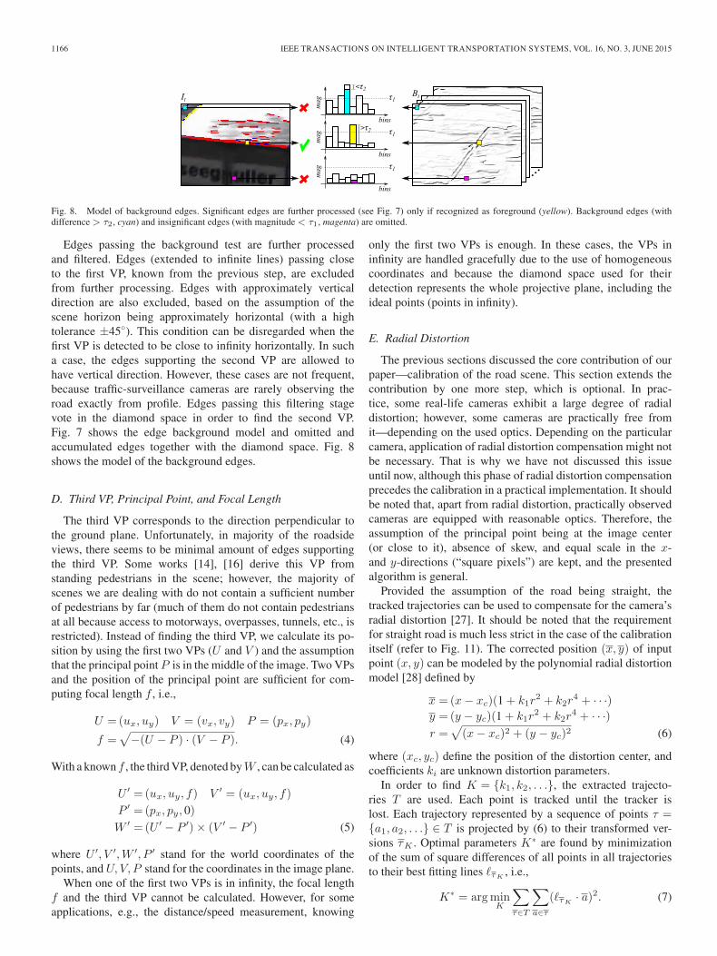
Fig. 8. Model of background edges. Significant edges are further processed (see Fig. 7) only if recognized as foreground (yellow). Background edges (withdifference > τ2, cyan) and insignificant edges (with magnitude < τ1, magenta) are omitted.
Edges passing the background test are further processedand filtered. Edges (extended to infinite lines) passing closeto the first VP, known from the previous step, are excludedfrom further processing. Edges with approximately verticaldirection are also excluded, based on the assumption of thescene horizon being approximately horizontal (with a hightolerance ±45◦). This condition can be disregarded when thefirst VP is detected to be close to infinity horizontally. In sucha case, the edges supporting the second VP are allowed tohave vertical direction. However, these cases are not frequent,because traffic-surveillance cameras are rarely observing theroad exactly from profile. Edges passing this filtering stagevote in the diamond space in order to find the second VP.Fig. 7 shows the edge background model and omitted andaccumulated edges together with the diamond space. Fig. 8shows the model of the background edges.
D. Third VP, Principal Point, and Focal Length
The third VP corresponds to the direction perpendicular tothe ground plane. Unfortunately, in majority of the roadsideviews, there seems to be minimal amount of edges supportingthe third VP. Some works [14], [16] derive this VP fromstanding pedestrians in the scene; however, the majority ofscenes we are dealing with do not contain a sufficient numberof pedestrians by far (much of them do not contain pedestriansat all because access to motorways, overpasses, tunnels, etc., isrestricted). Instead of finding the third VP, we calculate its po-sition by using the first two VPs (U and V ) and the assumptionthat the principal point P is in the middle of the image. Two VPsand the position of the principal point are sufficient for com-puting focal length f , i.e.,
U =(ux, uy) V = (vx, vy) P = (px, py)
f =√−(U − P ) · (V − P ). (4)
With a known f , the third VP, denoted byW , can be calculated as
U ′ =(ux, uy, f) V ′ = (ux, uy, f)
P ′ =(px, py, 0)
W ′ =(U ′ − P ′)× (V ′ − P ′) (5)
where U ′, V ′,W ′, P ′ stand for the world coordinates of thepoints, and U, V, P stand for the coordinates in the image plane.
When one of the first two VPs is in infinity, the focal lengthf and the third VP cannot be calculated. However, for someapplications, e.g., the distance/speed measurement, knowing
only the first two VPs is enough. In these cases, the VPs ininfinity are handled gracefully due to the use of homogeneouscoordinates and because the diamond space used for theirdetection represents the whole projective plane, including theideal points (points in infinity).
E. Radial Distortion
The previous sections discussed the core contribution of ourpaper—calibration of the road scene. This section extends thecontribution by one more step, which is optional. In prac-tice, some real-life cameras exhibit a large degree of radialdistortion; however, some cameras are practically free fromit—depending on the used optics. Depending on the particularcamera, application of radial distortion compensation might notbe necessary. That is why we have not discussed this issueuntil now, although this phase of radial distortion compensationprecedes the calibration in a practical implementation. It shouldbe noted that, apart from radial distortion, practically observedcameras are equipped with reasonable optics. Therefore, theassumption of the principal point being at the image center(or close to it), absence of skew, and equal scale in the x-and y-directions (“square pixels”) are kept, and the presentedalgorithm is general.
Provided the assumption of the road being straight, thetracked trajectories can be used to compensate for the camera’sradial distortion [27]. It should be noted that the requirementfor straight road is much less strict in the case of the calibrationitself (refer to Fig. 11). The corrected position (x, y) of inputpoint (x, y) can be modeled by the polynomial radial distortionmodel [28] defined by
x =(x− xc)(1 + k1r2 + k2r
4 + · · ·)y =(y − yc)(1 + k1r
2 + k2r4 + · · ·)
r =√
(x− xc)2 + (y − yc)2 (6)
where (xc, yc) define the position of the distortion center, andcoefficients ki are unknown distortion parameters.
In order to find K = {k1, k2, . . .}, the extracted trajecto-ries T are used. Each point is tracked until the tracker islost. Each trajectory represented by a sequence of points τ ={a1, a2, . . .} ∈ T is projected by (6) to their transformed ver-sions τK . Optimal parameters K∗ are found by minimizationof the sum of square differences of all points in all trajectoriesto their best fitting lines �τK
, i.e.,
K∗ = argminK
∑τ∈T
∑a∈τ
(�τK· a)2. (7)
DUBSKÁ et al.: FULLY AUTOMATIC ROADSIDE CAMERA CALIBRATION FOR TRAFFIC SURVEILLANCE 1167
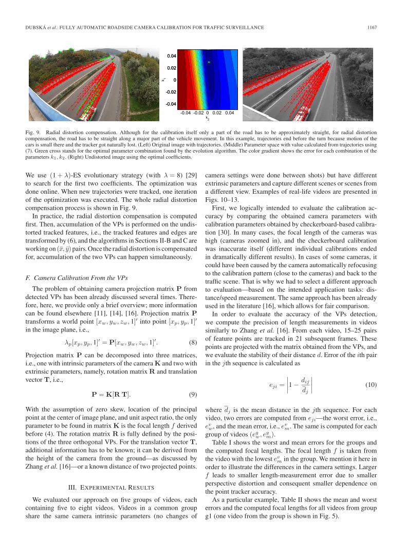
Fig. 9. Radial distortion compensation. Although for the calibration itself only a part of the road has to be approximately straight, for radial distortioncompensation, the road has to be straight along a major part of the vehicle movement. In this example, trajectories end before the turn because motion of thecars is small there and the tracker got naturally lost. (Left) Original image with trajectories. (Middle) Parameter space with value calculated from trajectories using(7). Green cross stands for the optimal parameter combination found by the evolution algorithm. The color gradient shows the error for each combination of theparameters k1, k2. (Right) Undistorted image using the optimal coefficients.
We use (1 + λ)-ES evolutionary strategy (with λ = 8) [29]to search for the first two coefficients. The optimization wasdone online. When new trajectories were tracked, one iterationof the optimization was executed. The whole radial distortioncompensation process is shown in Fig. 9.
In practice, the radial distortion compensation is computedfirst. Then, accumulation of the VPs is performed on the undis-torted tracked features, i.e., the tracked features and edges aretransformed by (6), and the algorithms in Sections II-B and C areworking on (x, y)pairs. Once the radial distortion is compensatedfor, accumulation of the two VPs can happen simultaneously.
F. Camera Calibration From the VPs
The problem of obtaining camera projection matrix P fromdetected VPs has been already discussed several times. There-fore, here, we provide only a brief overview; more informationcan be found elsewhere [11], [14], [16]. Projection matrix Ptransforms a world point [xw, yw, zw, 1]′ into point [xp, yp, 1]′
in the image plane, i.e.,
λp[xp, yp, 1]′ = P[xw, yw, zw, 1]′. (8)
Projection matrix P can be decomposed into three matrices,i.e., one with intrinsic parameters of the camera K and two withextrinsic parameters, namely, rotation matrix R and translationvector T, i.e.,
P = K[R T]. (9)
With the assumption of zero skew, location of the principalpoint at the center of image plane, and unit aspect ratio, the onlyparameter to be found in matrix K is the focal length f derivedbefore (4). The rotation matrix R is fully defined by the posi-tions of the three orthogonal VPs. For the translation vector T,additional information has to be known; it can be derived fromthe height of the camera from the ground—as discussed byZhang et al. [16]—or a known distance of two projected points.
III. EXPERIMENTAL RESULTS
We evaluated our approach on five groups of videos, eachcontaining five to eight videos. Videos in a common groupshare the same camera intrinsic parameters (no changes of
camera settings were done between shots) but have differentextrinsic parameters and capture different scenes or scenes froma different view. Examples of real-life videos are presented inFigs. 10–13.
First, we logically intended to evaluate the calibration ac-curacy by comparing the obtained camera parameters withcalibration parameters obtained by checkerboard-based calibra-tion [30]. In many cases, the focal length of the cameras washigh (cameras zoomed in), and the checkerboard calibrationwas inaccurate itself (different individual calibrations endedin dramatically different results). In cases of some cameras, itcould have been caused by the camera automatically refocusingto the calibration pattern (close to the cameras) and back to thetraffic scene. That is why we had to select a different approachto evaluation—based on the intended application tasks: dis-tance/speed measurement. The same approach has been alreadyused in the literature [16], which allows for fair comparison.
In order to evaluate the accuracy of the VPs detection,we compute the precision of length measurements in videossimilarly to Zhang et al. [16]. From each video, 15–25 pairsof feature points are tracked in 21 subsequent frames. Thesepoints are projected with the matrix obtained from the VPs, andwe evaluate the stability of their distance d. Error of the ith pairin the jth sequence is calculated as
eji =
∣∣∣∣1 − dij
dj
∣∣∣∣ (10)
where dj is the mean distance in the jth sequence. For eachvideo, two errors are computed from eji—the worst error, i.e.,evw, and the mean error, i.e., evm. The same is computed for eachgroup of videos (egw, e
gm).
Table I shows the worst and mean errors for the groups andthe computed focal lengths. The focal length f is taken fromthe video with the lowest evm in the group. We mention it here inorder to illustrate the differences in the camera settings. Largerf leads to smaller length-measurement error due to smallerperspective distortion and consequent smaller dependence onthe point tracker accuracy.
As a particular example, Table II shows the mean and worsterrors and the computed focal lengths for all videos from groupg1 (one video from the group is shown in Fig. 5).
1168 IEEE TRANSACTIONS ON INTELLIGENT TRANSPORTATION SYSTEMS, VOL. 16, NO. 3, JUNE 2015
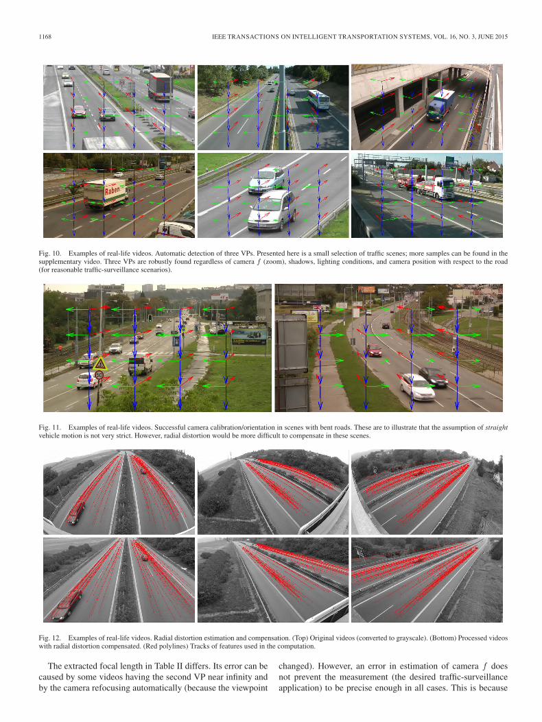
Fig. 10. Examples of real-life videos. Automatic detection of three VPs. Presented here is a small selection of traffic scenes; more samples can be found in thesupplementary video. Three VPs are robustly found regardless of camera f (zoom), shadows, lighting conditions, and camera position with respect to the road(for reasonable traffic-surveillance scenarios).
Fig. 11. Examples of real-life videos. Successful camera calibration/orientation in scenes with bent roads. These are to illustrate that the assumption of straightvehicle motion is not very strict. However, radial distortion would be more difficult to compensate in these scenes.
Fig. 12. Examples of real-life videos. Radial distortion estimation and compensation. (Top) Original videos (converted to grayscale). (Bottom) Processed videoswith radial distortion compensated. (Red polylines) Tracks of features used in the computation.
The extracted focal length in Table II differs. Its error can becaused by some videos having the second VP near infinity andby the camera refocusing automatically (because the viewpoint
changed). However, an error in estimation of camera f doesnot prevent the measurement (the desired traffic-surveillanceapplication) to be precise enough in all cases. This is because
DUBSKÁ et al.: FULLY AUTOMATIC ROADSIDE CAMERA CALIBRATION FOR TRAFFIC SURVEILLANCE 1169
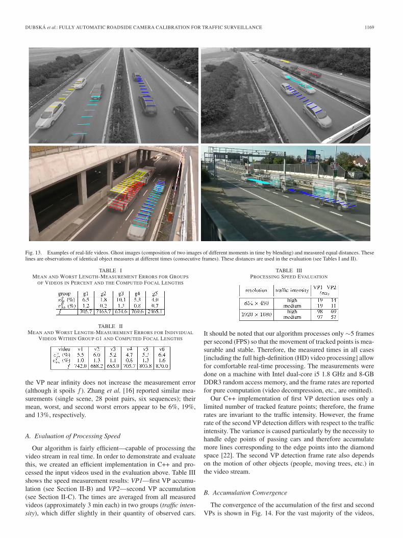
Fig. 13. Examples of real-life videos. Ghost images (composition of two images of different moments in time by blending) and measured equal distances. Theselines are observations of identical object measures at different times (consecutive frames). These distances are used in the evaluation (see Tables I and II).
TABLE IMEAN AND WORST LENGTH-MEASUREMENT ERRORS FOR GROUPS
OF VIDEOS IN PERCENT AND THE COMPUTED FOCAL LENGTHS
TABLE IIMEAN AND WORST LENGTH-MEASUREMENT ERRORS FOR INDIVIDUAL
VIDEOS WITHIN GROUP G1 AND COMPUTED FOCAL LENGTHS
the VP near infinity does not increase the measurement error(although it spoils f ). Zhang et al. [16] reported similar mea-surements (single scene, 28 point pairs, six sequences); theirmean, worst, and second worst errors appear to be 6%, 19%,and 13%, respectively.
A. Evaluation of Processing Speed
Our algorithm is fairly efficient—capable of processing thevideo stream in real time. In order to demonstrate and evaluatethis, we created an efficient implementation in C++ and pro-cessed the input videos used in the evaluation above. Table IIIshows the speed measurement results: VP1—first VP accumu-lation (see Section II-B) and VP2—second VP accumulation(see Section II-C). The times are averaged from all measuredvideos (approximately 3 min each) in two groups (traffic inten-sity), which differ slightly in their quantity of observed cars.
TABLE IIIPROCESSING SPEED EVALUATION
It should be noted that our algorithm processes only ∼5 framesper second (FPS) so that the movement of tracked points is mea-surable and stable. Therefore, the measured times in all cases[including the full high-definition (HD) video processing] allowfor comfortable real-time processing. The measurements weredone on a machine with Intel dual-core i5 1.8 GHz and 8-GBDDR3 random access memory, and the frame rates are reportedfor pure computation (video decompression, etc., are omitted).
Our C++ implementation of first VP detection uses only alimited number of tracked feature points; therefore, the framerates are invariant to the traffic intensity. However, the framerate of the second VP detection differs with respect to the trafficintensity. The variance is caused particularly by the necessity tohandle edge points of passing cars and therefore accumulatemore lines corresponding to the edge points into the diamondspace [22]. The second VP detection frame rate also dependson the motion of other objects (people, moving trees, etc.) inthe video stream.
B. Accumulation Convergence
The convergence of the accumulation of the first and secondVPs is shown in Fig. 14. For the vast majority of the videos,
1170 IEEE TRANSACTIONS ON INTELLIGENT TRANSPORTATION SYSTEMS, VOL. 16, NO. 3, JUNE 2015
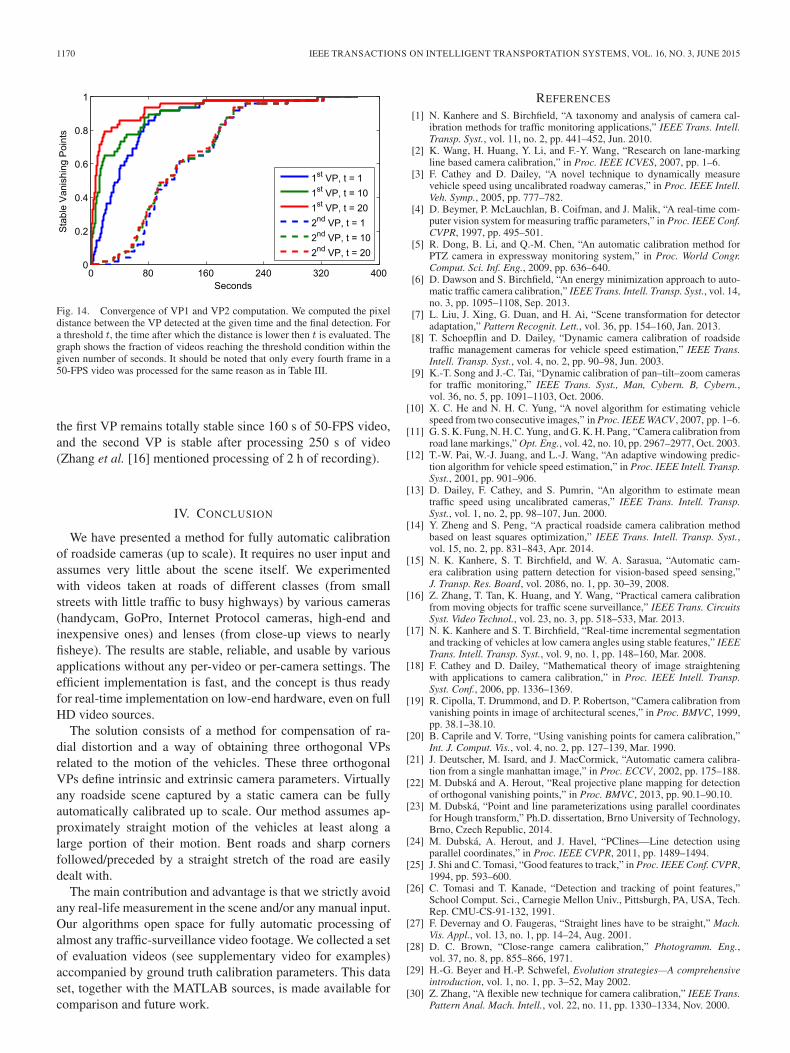
Fig. 14. Convergence of VP1 and VP2 computation. We computed the pixeldistance between the VP detected at the given time and the final detection. Fora threshold t, the time after which the distance is lower then t is evaluated. Thegraph shows the fraction of videos reaching the threshold condition within thegiven number of seconds. It should be noted that only every fourth frame in a50-FPS video was processed for the same reason as in Table III.
the first VP remains totally stable since 160 s of 50-FPS video,and the second VP is stable after processing 250 s of video(Zhang et al. [16] mentioned processing of 2 h of recording).
IV. CONCLUSION
We have presented a method for fully automatic calibrationof roadside cameras (up to scale). It requires no user input andassumes very little about the scene itself. We experimentedwith videos taken at roads of different classes (from smallstreets with little traffic to busy highways) by various cameras(handycam, GoPro, Internet Protocol cameras, high-end andinexpensive ones) and lenses (from close-up views to nearlyfisheye). The results are stable, reliable, and usable by variousapplications without any per-video or per-camera settings. Theefficient implementation is fast, and the concept is thus readyfor real-time implementation on low-end hardware, even on fullHD video sources.
The solution consists of a method for compensation of ra-dial distortion and a way of obtaining three orthogonal VPsrelated to the motion of the vehicles. These three orthogonalVPs define intrinsic and extrinsic camera parameters. Virtuallyany roadside scene captured by a static camera can be fullyautomatically calibrated up to scale. Our method assumes ap-proximately straight motion of the vehicles at least along alarge portion of their motion. Bent roads and sharp cornersfollowed/preceded by a straight stretch of the road are easilydealt with.
The main contribution and advantage is that we strictly avoidany real-life measurement in the scene and/or any manual input.Our algorithms open space for fully automatic processing ofalmost any traffic-surveillance video footage. We collected a setof evaluation videos (see supplementary video for examples)accompanied by ground truth calibration parameters. This dataset, together with the MATLAB sources, is made available forcomparison and future work.
REFERENCES
[1] N. Kanhere and S. Birchfield, “A taxonomy and analysis of camera cal-ibration methods for traffic monitoring applications,” IEEE Trans. Intell.Transp. Syst., vol. 11, no. 2, pp. 441–452, Jun. 2010.
[2] K. Wang, H. Huang, Y. Li, and F.-Y. Wang, “Research on lane-markingline based camera calibration,” in Proc. IEEE ICVES, 2007, pp. 1–6.
[3] F. Cathey and D. Dailey, “A novel technique to dynamically measurevehicle speed using uncalibrated roadway cameras,” in Proc. IEEE Intell.Veh. Symp., 2005, pp. 777–782.
[4] D. Beymer, P. McLauchlan, B. Coifman, and J. Malik, “A real-time com-puter vision system for measuring traffic parameters,” in Proc. IEEE Conf.CVPR, 1997, pp. 495–501.
[5] R. Dong, B. Li, and Q.-M. Chen, “An automatic calibration method forPTZ camera in expressway monitoring system,” in Proc. World Congr.Comput. Sci. Inf. Eng., 2009, pp. 636–640.
[6] D. Dawson and S. Birchfield, “An energy minimization approach to auto-matic traffic camera calibration,” IEEE Trans. Intell. Transp. Syst., vol. 14,no. 3, pp. 1095–1108, Sep. 2013.
[7] L. Liu, J. Xing, G. Duan, and H. Ai, “Scene transformation for detectoradaptation,” Pattern Recognit. Lett., vol. 36, pp. 154–160, Jan. 2013.
[8] T. Schoepflin and D. Dailey, “Dynamic camera calibration of roadsidetraffic management cameras for vehicle speed estimation,” IEEE Trans.Intell. Transp. Syst., vol. 4, no. 2, pp. 90–98, Jun. 2003.
[9] K.-T. Song and J.-C. Tai, “Dynamic calibration of pan–tilt–zoom camerasfor traffic monitoring,” IEEE Trans. Syst., Man, Cybern. B, Cybern.,vol. 36, no. 5, pp. 1091–1103, Oct. 2006.
[10] X. C. He and N. H. C. Yung, “A novel algorithm for estimating vehiclespeed from two consecutive images,” in Proc. IEEE WACV , 2007, pp. 1–6.
[11] G. S. K. Fung, N. H. C. Yung, and G. K. H. Pang, “Camera calibration fromroad lane markings,” Opt. Eng., vol. 42, no. 10, pp. 2967–2977, Oct. 2003.
[12] T.-W. Pai, W.-J. Juang, and L.-J. Wang, “An adaptive windowing predic-tion algorithm for vehicle speed estimation,” in Proc. IEEE Intell. Transp.Syst., 2001, pp. 901–906.
[13] D. Dailey, F. Cathey, and S. Pumrin, “An algorithm to estimate meantraffic speed using uncalibrated cameras,” IEEE Trans. Intell. Transp.Syst., vol. 1, no. 2, pp. 98–107, Jun. 2000.
[14] Y. Zheng and S. Peng, “A practical roadside camera calibration methodbased on least squares optimization,” IEEE Trans. Intell. Transp. Syst.,vol. 15, no. 2, pp. 831–843, Apr. 2014.
[15] N. K. Kanhere, S. T. Birchfield, and W. A. Sarasua, “Automatic cam-era calibration using pattern detection for vision-based speed sensing,”J. Transp. Res. Board, vol. 2086, no. 1, pp. 30–39, 2008.
[16] Z. Zhang, T. Tan, K. Huang, and Y. Wang, “Practical camera calibrationfrom moving objects for traffic scene surveillance,” IEEE Trans. CircuitsSyst. Video Technol., vol. 23, no. 3, pp. 518–533, Mar. 2013.
[17] N. K. Kanhere and S. T. Birchfield, “Real-time incremental segmentationand tracking of vehicles at low camera angles using stable features,” IEEETrans. Intell. Transp. Syst., vol. 9, no. 1, pp. 148–160, Mar. 2008.
[18] F. Cathey and D. Dailey, “Mathematical theory of image straighteningwith applications to camera calibration,” in Proc. IEEE Intell. Transp.Syst. Conf., 2006, pp. 1336–1369.
[19] R. Cipolla, T. Drummond, and D. P. Robertson, “Camera calibration fromvanishing points in image of architectural scenes,” in Proc. BMVC, 1999,pp. 38.1–38.10.
[20] B. Caprile and V. Torre, “Using vanishing points for camera calibration,”Int. J. Comput. Vis., vol. 4, no. 2, pp. 127–139, Mar. 1990.
[21] J. Deutscher, M. Isard, and J. MacCormick, “Automatic camera calibra-tion from a single manhattan image,” in Proc. ECCV , 2002, pp. 175–188.
[22] M. Dubská and A. Herout, “Real projective plane mapping for detectionof orthogonal vanishing points,” in Proc. BMVC, 2013, pp. 90.1–90.10.
[23] M. Dubská, “Point and line parameterizations using parallel coordinatesfor Hough transform,” Ph.D. dissertation, Brno University of Technology,Brno, Czech Republic, 2014.
[24] M. Dubská, A. Herout, and J. Havel, “PClines—Line detection usingparallel coordinates,” in Proc. IEEE CVPR, 2011, pp. 1489–1494.
[25] J. Shi and C. Tomasi, “Good features to track,” in Proc. IEEE Conf. CVPR,1994, pp. 593–600.
[26] C. Tomasi and T. Kanade, “Detection and tracking of point features,”School Comput. Sci., Carnegie Mellon Univ., Pittsburgh, PA, USA, Tech.Rep. CMU-CS-91-132, 1991.
[27] F. Devernay and O. Faugeras, “Straight lines have to be straight,” Mach.Vis. Appl., vol. 13, no. 1, pp. 14–24, Aug. 2001.
[28] D. C. Brown, “Close-range camera calibration,” Photogramm. Eng.,vol. 37, no. 8, pp. 855–866, 1971.
[29] H.-G. Beyer and H.-P. Schwefel, Evolution strategies—A comprehensiveintroduction, vol. 1, no. 1, pp. 3–52, May 2002.
[30] Z. Zhang, “A flexible new technique for camera calibration,” IEEE Trans.Pattern Anal. Mach. Intell., vol. 22, no. 11, pp. 1330–1334, Nov. 2000.
DUBSKÁ et al.: FULLY AUTOMATIC ROADSIDE CAMERA CALIBRATION FOR TRAFFIC SURVEILLANCE 1171
Markéta Dubská received the Ph.D. degree fromBrno University of Technology (BUT), Brno, CzechRepublic, in 2014.
She is a Postdoctoral Fellow with the Departmentof Computer Graphics and Multimedia, Faculty ofInformation Technology, BUT. Her research interestsinclude computer vision, geometry, and computationusing parallel coordinates.
Adam Herout received the Ph.D. degree fromBrno University of Technology (BUT), Brno, CzechRepublic.
He is an Associate Professor with BUT, wherehe also leads the Graph@FIT Research Group. Hisresearch interests include fast algorithms and hard-ware acceleration in computer vision. He is also aCofounder of angelcam.com, which provides webstreaming from network cameras and real-time com-puter vision in the cloud.
Roman Juránek received the Ph.D. degree fromBrno University of Technology (BUT), Brno, CzechRepublic, in 2012.
He is currently a Postdoctoral Fellow with theGraph@FIT Research Group, Department of Com-puter Graphics and Multimedia, Faculty of Infor-mation Technology, BUT. His professional interestsinclude computer vision, machine learning, and pat-tern recognition.
Jakub Sochor received the M.S. degree fromBrno University of Technology (BUT), Brno, CzechRepublic. He is currently working toward the Ph.D.degree in the Department of Computer Graph-ics and Multimedia, Faculty of Information Tech-nology, BUT.
His research focuses on computer vision, particu-larly traffic surveillance.