Markups as a Hedge for Input Price Uncertainty: Evidence ...

Research Institute of Industrial Economics

P.O. Box 55665

SE-102 15 Stockholm, Sweden

[email protected]

www.ifn.se

IFN Working Paper No. 1418, 2021

Markups as a Hedge for Input Price Uncertainty: Evidence from Sweden Sneha Agrawal, Abhishek Gaurav and Melinda Suveg

Markups as a Hedge for Input Price Uncertainty:

Evidence from Sweden

Sneha Agrawal*, Abhishek Gaurav�, Melinda Suveg�§

November 5, 2021

In this paper, we study a new channel to explain firms’ price setting behavior. We propose

that uncertainty about factor prices has a positive effect on markups. We show theoreti-

cally that firms with higher shares of inputs with volatile prices set higher markups. We

use the Bartik shift-share approach to empirically test whether firms which use more oil

relative to other inputs set higher markups when oil prices are more volatile. Our esti-

mates imply that a one standard deviation increase in oil price volatility leads to a 0.38

percent increase in the markup of firms with average oil exposure.

JEL classification: D21, D22, D24, D42, D80, E31, E32, L11, L60.

Keywords: price setting, markups, input price volatility, precautionary pricing.

*International Monetary Fund, [email protected]�Princeton University, [email protected]�Contact: [email protected], Research Institute of Industrial Economics (IFN), P.O. Box 55665,

SE-102 15 Stockholm, Sweden.§Acknowledgments: We would like to thank Nils Gottfries, Simon Gilchrist, Stefan Pitschner, Mikael

Carlsson and Plamen T. Nenov for their helpful comments and guidance. We would like to thankthe seminar participants at Uppsala University for their comments and suggestions. Melinda Suvegacknowledges funding from the Marianne and Marcus Wallenberg Foundation (2020.0049) and wouldalso like to thank the Department of Economics at Uppsala University and Jan Wallanders och TomHedelius stiftelse for the financial support.

1

1 Introduction

Markups are at the center of attention for their connection to rising profits, the decline

in the labor share, and the increase in inequality between capital owners and workers. In

this paper, we propose a new channel to explain firms’ price setting behavior. We argue

that uncertainty about factor prices has a positive effect on markups. By examining this

new channel, our paper contributes to understanding the way in which firms set markups

and the reasons why markups differ across firms.

First, we build a model to formalize the argument that uncertainty about factor prices

leads to higher markups. We augment a simple version of the Dixit and Stiglitz (1977)

model of competition with a stochastic marginal cost of production. The new mechanism

we include in our model posits that firms set higher markups to hedge against negative

profits that could result if firms’ variable costs turn out to be high. In our model, firms

are averse to negative profits because they are required to pay an additional penalty

that is proportional to the amount by which dividends fall short of a threshold value.

This threshold value can be interpreted as the cost of raising equity to finance negative

values of dividends (Gilchrist, Schoenle, Sim and Zakrajsek, 2017) or the high cost of

debt issuance via borrowing covenants (Lian and Ma, 2020). Our model shows that the

exposure of firms to the price volatility of major inputs matters for the determination of

firm-level markups. In particular, we find that firms with higher shares of inputs with

volatile prices in their total variable costs set higher markups.

Then, we test the implications of our model empirically. Our hypothesis is that firm-

level markups increase with the volatility of input prices faced by firms. We use a Bartik

shift-share approach for our empirical strategy. Specifically, we measure the exposure of

firms to oil price volatility and we test whether firms with higher exposures set higher

markups when oil prices are more volatile.

We construct markups using current methods developed by De Loecker and Warzynski

(2012) and Ackerberg, Caves and Frazer (2015). We measure firms’ exposure to input

price volatility by their industry’s cost for oil relative to their industry’s variable cost.

To measure uncertainty in oil prices, we construct a forward-looking measure of expected

volatility using firms’ available information set at the time when they make their pricing

decisions. We consider a simple GARCH model to construct an annual measure of the

2

expected standard deviation of monthly Brent oil price changes.1

For identification with the Bartik shift-share approach, we follow Goldsmith-Pinkham,

Sorkin and Swift (2020) and argue for the exogeneity of the oil shares. The crucial

identifying assumption we make is that changes in demand that correlate with oil price

volatility do not differentially affect firms in industries with higher oil shares, given the

control variables. By having the markup rather than the price as the dependent variable,

we eliminate the direct effect of cost shocks on prices and we isolate the effect of input

price volatility on markups.

We find that a one standard deviation increase in volatility leads to a 0.38 percent

increase in the markup of firms with average oil exposure. The effect is stronger for firms

with high oil exposure. A one standard deviation increase in volatility leads to a 1.98

percent increase of the markup of firms with industry oil exposure in the 95th percentile

versus only 0.05 percent for firms with industry oil exposure in the 5th percentile. A

number of robustness checks also yield coefficients around 0.4 percent. The average

within-industry change in markups is about 4 percent, suggesting that our proposed

channel explains one tenth of the average markup variation.

Our paper is most related to the literature that studies the relation between input

costs, markups and prices. De Loecker, Goldberg, Khandelwal and Pavcnik (2016) ana-

lyze how an increase in input costs affects markups. Born and Pfeifer (2021) show that

an increase in uncertainty about the aggregate price level induces a rise in markups. In

terms of price dispersion, Klepacz (2020) shows that higher oil price volatility leads to

higher industry-level price dispersion. The novelty of our paper is that we look at the

effect of input price volatility on levels of markups.

Our analysis intersects with three strands of literature. Much recent research has

focused on the impact of uncertainty on firms’ choices of quantities of inputs, output

and investment. This research goes back to papers on uncertainty and investment by Oi

(1961), Abel (1983), Hartman (1972) and more recently by Bloom (2009) and Bai, Kehoe

and Arellano (2011). We depart from this strand of papers since we look at the impact

of uncertainty on markups and prices, not the quantity choice.

Another strand of research has studied markups, often finding large and rising markups

(De Loecker, Eeckhout and Unger, 2020) and a decline in the labor share (Karabarbou-

1We use uncertainty and volatility about input prices interchangeably when referring to the mecha-nism. In the data, volatility is measured by the expected standard deviation.

3

nis and Neiman, 2014). This literature has focused on the measurement of markups and

their economic interpretations (De Loecker and Warzynski, 2012; Nakamura and Zerom,

2010; Gutierrez and Philippon, 2017; Karabarbounis and Neiman, 2018; De Loecker et

al., 2020). Similarly to these papers, we construct markups from data, but we aim to

investigate the impact of input price volatility on markups.

We also intersect with the literature on precautionary behavior and relate to the

papers on borrowing covenants by Lian and Ma (2020) and Gilchrist et al. (2017) who

consider implicit costs of external financing for firms. Our model includes a reduced form

version of costly external financing which can be rationalized using the arguments in Lian

and Ma (2020) and Gilchrist et al. (2017).

This paper is structured as follows. Section 2 describes the theoretical framework.

Section 3 explains the method and data used for our empirical analysis. Section 4 explains

the main results and section 5 presents the robustness checks. Section 6 concludes the

paper.

2 Theory

To develop the argument for increasing markups from higher volatility of major inputs,

we consider a simple version of the Dixit and Stiglitz (1977) model of competition with a

stochastic marginal cost of production. The economy consists of a representative house-

hold and representative firms in j industries.

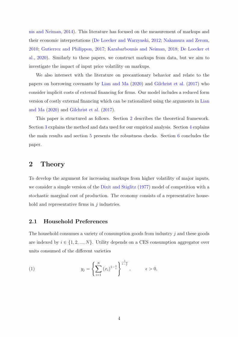
2.1 Household Preferences

The household consumes a variety of consumption goods from industry j and these goods

are indexed by i ∈ {1, 2, ..., N}. Utility depends on a CES consumption aggregator over

units consumed of the different varieties

(1) yj =

{N∑i=1

(xi)1− 1

ϵ

} 1

1− 1ϵ

, ϵ > 0,

4

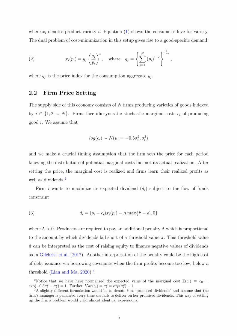
where xi denotes product variety i. Equation (1) shows the consumer’s love for variety.

The dual problem of cost-minimization in this setup gives rise to a good-specific demand,

(2) xi(pi) = yj

(qjpi

)ϵ

, where qj =

{N∑i=1

(pi)1−ϵ

} 11−ϵ

,

where qj is the price index for the consumption aggregate yj.

2.2 Firm Price Setting

The supply side of this economy consists of N firms producing varieties of goods indexed

by i ∈ {1, 2, ..., N}. Firms face idiosyncratic stochastic marginal costs ci of producing

good i. We assume that

log(ci) ∼ N(µi = −0.5σ2i , σ

2i )

and we make a crucial timing assumption that the firm sets the price for each period

knowing the distribution of potential marginal costs but not its actual realization. After

setting the price, the marginal cost is realized and firms learn their realized profits as

well as dividends.2

Firm i wants to maximize its expected dividend (di) subject to the flow of funds

constraint

(3) di = (pi − ci)xi(pi)− Λmax{π − di, 0}

where Λ > 0. Producers are required to pay an additional penalty Λ which is proportional

to the amount by which dividends fall short of a threshold value π. This threshold value

π can be interpreted as the cost of raising equity to finance negative values of dividends

as in Gilchrist et al. (2017). Another interpretation of the penalty could be the high cost

of debt issuance via borrowing covenants when the firm profits become too low, below a

threshold (Lian and Ma, 2020).3

2Notice that we have have normalized the expected value of the marginal cost E(ci) ≡ c0 =exp(−0.5σ2

i + σ2i ) = 1. Further, V ar(ci) = σ2

i = exp(σ2i )− 1

3A slightly different formulation would be to denote π as ’promised dividends’ and assume that thefirm’s manager is penalized every time she fails to deliver on her promised dividends. This way of settingup the firm’s problem would yield almost identical expressions.

5

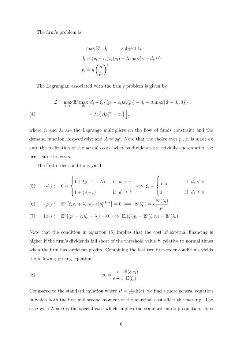
The firm’s problem is

maxEc [di] subject to

di = (pi − ci)xi(pi)− Λmax{π − di, 0}

xi = y

(q

pi

)ϵ

The Lagrangian associated with the firm’s problem is given by

L = maxpi,xi

Ecmaxdi

[di + ξi

{(pi − ci)xi(pi)− di − Λmax{π − di, 0}

}+ λi

{Ap−ϵ

i − xi

} ],(4)

where ξi and λi are the Lagrange multipliers on the flow of funds constraint and the

demand function, respectively; and A ≡ yqϵ. Note that the choice over pi, xi is made ex

ante the realization of the actual costs, whereas dividends are trivially chosen after the

firm learns its costs.

The first-order conditions yield

{di} : 0 =

1 + ξi(−1 + Λ) if di < π

1 + ξi(−1) if di ≥ π

=⇒ ξi =

1

1−Λif di < π

1 if di ≥ π

(5)

{pi} : Ec[ξixi + λiA(−ϵ)p−1−ϵ

i

]= 0 =⇒ Ec(ξi) = ϵ

Ec(λi)

pi(6)

{xi} : Ec [(pi − ci)ξi − λi] = 0 =⇒ Et(ξi)pi − Ec(ξici) = Ec(λi)(7)

Note that the condition in equation (5) implies that the cost of external financing is

higher if the firm’s dividends fall short of the threshold value π, relative to normal times

when the firm has sufficient profits. Combining the last two first-order conditions yields

the following pricing equation

pi =ϵ

ϵ− 1

E(ξici)E(ξi)

.(8)

Compared to the standard equation where P = ϵϵ−1

E(c), we find a more general equation

in which both the first and second moment of the marginal cost affect the markup. The

case with Λ = 0 is the special case which implies the standard markup equation. It is

6

easier to understand the underlying workings of this model in the (p, c) plane instead of

the (π, p) plane. Hence, we shall reformulate the problem in order to solve it analytically

in a more tractable manner.

Let c be the idiosyncratic cost level such that, at c, the firm’s flow of funds constraint

is binding with dividends equal to π. Then,

ci(pi) = pi −π

xi(pi)

Then, we get the equivalence that cit ≶ ci(pi) ⇐⇒ di(pi) ≶ π, so we can simplify

the expressions in the price equation above to get that

E(ξi) =c(pi)∫0

dF (ci) +

∞∫ci(pi)

1

1− ΛdF (ci)

= 1 +Λ

1− Λ(1− Φ(z(pi)) ,

where z(pi) ≡ (log c(pi) − µi)1σi

and Φ is the cumulative distribution function for the

normally distributed variable z(pi). Then, it is possible to re-write Ec(ξici) as

Ec(ξici) =

c(pi)∫0

cidF (ci) +

∞∫ci(pi)

1

1− ΛcidF (ci)

= c0 +Λ

1− ΛE (ci|ci ≥ c(pi)) (1− Φ(z(pi)) ,(9)

where the second term on the right-hand side is the probability of having a cost realization

larger than the threshold cost c times the expected cost. Given a positive penalty Λ > 0,

the firm puts extra weight on the high-cost states. Together, this implies the following

7

pricing equation

(10) pi =ϵ

ϵ− 1

c0 +Λ

1−ΛE (ci|ci ≥ c(pi)) (1− Φ(z(pi))

1 + Λ1−Λ

(1− Φ(z(pi)).

The solution to this fixed point problem yields the optimal price p∗i charged by the firm

as

(11) p∗i =ϵ

ϵ− 1

c0 +Λ

1−ΛE (ci|ci ≥ c(p∗it)) (1− Φ(z(p∗i ))

1 + Λ1−Λ

(1− Φ(z(p∗i )).

Next, we can use the formula for conditional expectation of a log normally distributed

variable4

Ec{ci|ci ≥ c(pi)} = exp

(µ+

σ2

2

) Φ(

µ+σ2−log(c(pi))σ

)1− Φ

(log c(pi)−µ

σ

)=

Φ(−z(pi) + σ)

1− Φ(z(pi))=

1− Φ(z(pi)− σ)

1− Φ(z(pi)),(12)

where σ is the standard deviation of the log normally distributed variable ci and µ is its

mean. We substitute (12) in equation (11) to find that the denominator in (12) cancels

out with the RHS term of the numerator in (11) and obtain that

(13) p∗i =ϵ

ϵ− 1

1 + Λ1−Λ

(1− Φ (z(p∗it)− σ))

1 + Λ1−Λ

(1− Φ (z(p∗it)))c0.

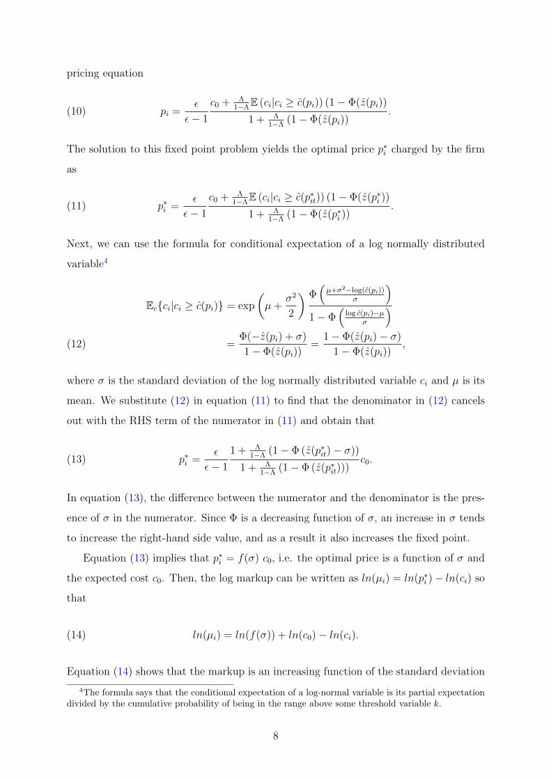
In equation (13), the difference between the numerator and the denominator is the pres-

ence of σ in the numerator. Since Φ is a decreasing function of σ, an increase in σ tends

to increase the right-hand side value, and as a result it also increases the fixed point.

Equation (13) implies that p∗i = f(σ) c0, i.e. the optimal price is a function of σ and

the expected cost c0. Then, the log markup can be written as ln(µi) = ln(p∗i )− ln(ci) so

that

(14) ln(µi) = ln(f(σ)) + ln(c0)− ln(ci).

Equation (14) shows that the markup is an increasing function of the standard deviation

4The formula says that the conditional expectation of a log-normal variable is its partial expectationdivided by the cumulative probability of being in the range above some threshold variable k.

8

of the volatile input.

2.3 Micro-founding marginal costs and volatility

We assume that the firm produces using Cobb-Douglas technology with oil mo and an-

other variable input mw. We also assume that firms within industry j use the same oil

input mix in their production so that if firm i belongs to industry j, then good xi is

produced according to

xi = zmαjo m1−αj

w ,

where z denotes the firm’s productivity and αj is the share of oil in the firm’s production

that only differs across industries. The firm minimizes its costs subject to its technology.

(15) minmo,mwV mo +Wmw + ηj(xi − zmαjo m1−αj

w )

where ηj is the Lagrange multiplier on the production function, the price of oil is V and

the price of the other variable input is W . The first-order conditions are

(16) V = αjηjxi

mo

, and W = (1− αj)ηjx

mw

.

Using these first-order conditions, we find that the total cost is the product of the marginal

cost ηj and the quantity produced

(17) V mo +Wmw = ηjxi

Raising each first-order condition to the respective share and multiplying yields the

marginal cost

(18) ηj =1

z

(V

αj

)αj(

W

1− αj

)1−αj

.

This implies that the standard deviation of the log marginal cost caused by variations in

oil prices is

(19) ση = αj σv,

9

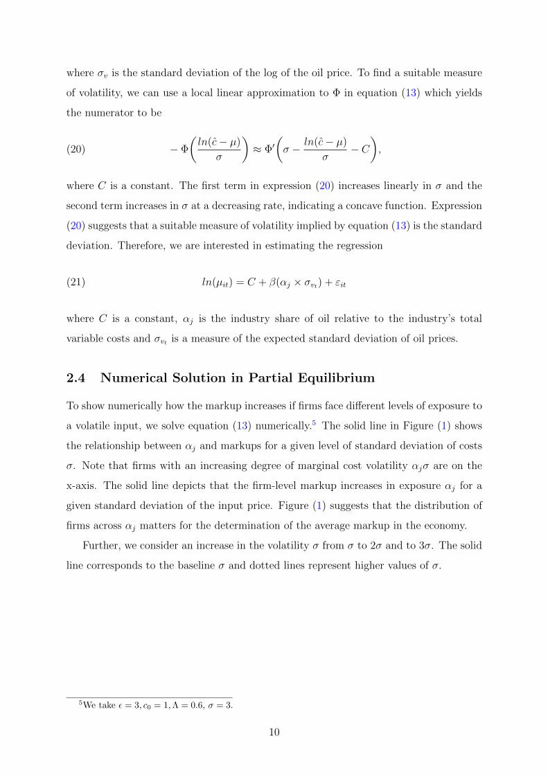
where σv is the standard deviation of the log of the oil price. To find a suitable measure

of volatility, we can use a local linear approximation to Φ in equation (13) which yields

the numerator to be

(20) − Φ

(ln(c− µ)

σ

)≈ Φ′

(σ − ln(c− µ)

σ− C

),

where C is a constant. The first term in expression (20) increases linearly in σ and the

second term increases in σ at a decreasing rate, indicating a concave function. Expression

(20) suggests that a suitable measure of volatility implied by equation (13) is the standard

deviation. Therefore, we are interested in estimating the regression

(21) ln(µit) = C + β(αj × σvt) + εit

where C is a constant, αj is the industry share of oil relative to the industry’s total

variable costs and σvt is a measure of the expected standard deviation of oil prices.

2.4 Numerical Solution in Partial Equilibrium

To show numerically how the markup increases if firms face different levels of exposure to

a volatile input, we solve equation (13) numerically.5 The solid line in Figure (1) shows

the relationship between αj and markups for a given level of standard deviation of costs

σ. Note that firms with an increasing degree of marginal cost volatility αjσ are on the

x-axis. The solid line depicts that the firm-level markup increases in exposure αj for a

given standard deviation of the input price. Figure (1) suggests that the distribution of

firms across αj matters for the determination of the average markup in the economy.

Further, we consider an increase in the volatility σ from σ to 2σ and to 3σ. The solid

line corresponds to the baseline σ and dotted lines represent higher values of σ.

5We take ϵ = 3, c0 = 1,Λ = 0.6, σ = 3.

10

Figure 1: Markups as a function of oil shares αj and input cost volatility σ.

The increase in the dashed lines relative to the solid line in Figure 1 shows that firms

with extremely low or high exposure respond less to increases in volatility than firms with

moderate exposure. In addition, firms with the lowest exposures are affected the most

when their exposure increases as compared to firms at the highest end. This effect is due

to the concavity of markups in exposure.

3 Method and Data

3.1 Empirical Regression

Our main regression specification is

(22) ln(µi,t) = β

(OiljTV Cj

× E[SDt]

)+ δj + γt + εi,t,

whereOiljTV Cj

is a two-digit manufacturing industry j’s nominal oil consumption over the

industry’s nominal variable cost. In the baseline estimation, we use the industry’s oil

consumption to variable cost ratio in 2008, i.e. in the first year of the sample. As a

robustness check, we use the industry time-average variable defined as 1T

∑T=2016t=2008

Oilj,tTV Cj,t

as a measure of exposure in an alternative specification.

E[SDt] is the annual expected volatility of monthly Brent oil price changes derived

11

from a GARCH model. A detailed description of these variables follows below.

In (22), industry fixed effects δj control for time-invariant industry-specific unobserved

confounding variables and year fixed effects γt take care of variation in general economic

conditions over time.

3.2 Firm population and industries

In the Swedish business registry, some firms may be inactive or serve purely legal purposes,

for example companies that manage savings and investments of individuals. In order to

focus on economically active firms and eliminate companies that do not participate in

production, we consider firms with more than ten employees and positive sales. As

a robustness check, we include firms with more than two employees. We focus on an

unbalanced panel of firms in the manufacturing industry between 2008-2016.

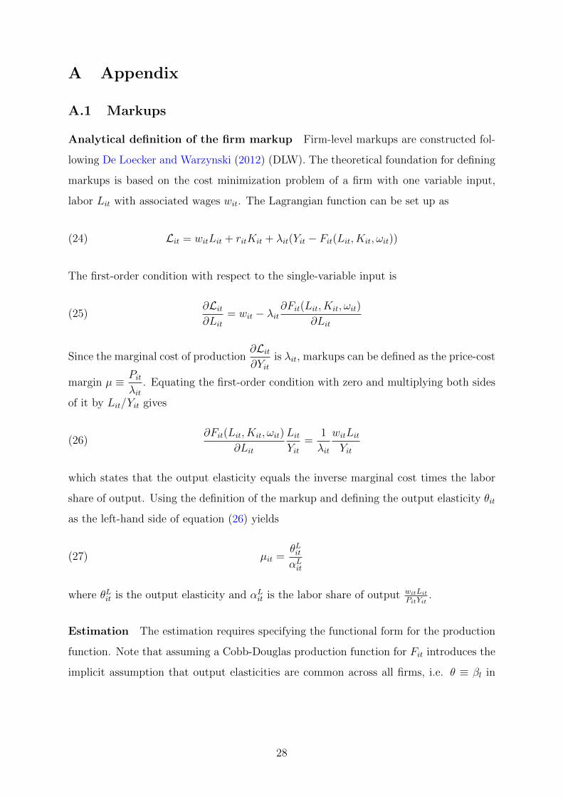
3.3 Markups

Firm-level markups are constructed following De Loecker and Warzynski (2012) based on

estimating a value added production function as in Ackerberg, Caves and Frazer (2015).

The theoretical foundation for defining markups is the cost minimization problem of

the firm. We closely follow the steps described by De Loecker and Warzynski (2012)

and Ackerberg et al. (2015) to construct markups and we include a description of our

procedures in Appendix A.1.

In the regression, we consider two sets of markups that we construct using (i) the

Cobb-Douglas and (ii) the translog production functions.6 Table 1 presents the summary

statistics for firm-level markups. While the average markup is similar across the Cobb-

Douglas and the translog specifications, the range of estimated markups is much wider

when the markups are based on the translog production function.

6Note that constructing markups as the labor share over sales would not be appropriate for theregressions since sales are price times quantity where prices vary endogenously with costs.

12

Table 1: Summary statistics: markups

Mean SD p5 p50 p95

Markup of firms with > 2 employeesmarkupCD 1.63 0.32 1.29 1.58 2.17markupTL 1.83 1.16 0.68 1.31 3.98Markup of firms with > 10 employeesmarkupCD 1.66 0.34 1.29 1.61 2.25markupTL 1.92 1.26 0.58 1.37 4.25

It is important to note that the markups based on the Cobb-Douglas production

function are only slightly different from the firm’s labor share relative to the firm’s value

added output by an industry-specific constant θj, i.e. the industry-specific output elas-

ticity. This feature of the Cobb-Douglas markups implies that the variation used in

estimating (22) is simply the variation in the firm-level labor share relative to the firm’s

value added output over time and differences across industries due to the elasticity of

output to inputs are soaked up by the industry fixed effects.

On the other hand, translog markups have a time-firm specific elasticity of output

component,7 which is why regression (22) with translog markups can utilize further vari-

ation in the dependent variable that is not soaked up by the industry fixed effects.

3.4 Volatility of oil prices

The annual volatility of oil prices is measured by the expected standard deviation of

monthly Brent oil price changes from a GARCH model. We use the data on monthly

crude oil spot prices for Brent in Europe because it is used as a reference for pricing a

number of oil products used by the Swedish firms as input. We collect the monthly price

series for dollars per barrel from FRED data. It can be argued that changes in Brent oil

price volatility are plausibly exogenous to Swedish firms. The oil price series are deflated

using finished goods US PPI to get the real oil prices

P oil =Brent Spot pricet

PPIt.

We want to consider the volatility in input prices that the firms expect when making

7The output elasticity based on the translog production function takes the form of expression (30) inappendix A.1.

13

output pricing decisions. Therefore, it is important to consider a forward-looking measure

of expected volatility using the information set available to firms at the time when they

make their pricing decisions. To model expected volatility in oil prices, we use a simple

GARCH model on oil price returns.

Let us define the monthly return on the Brent oil spot price for time period t as

roilt = logP oilt − logP oil

t−1.

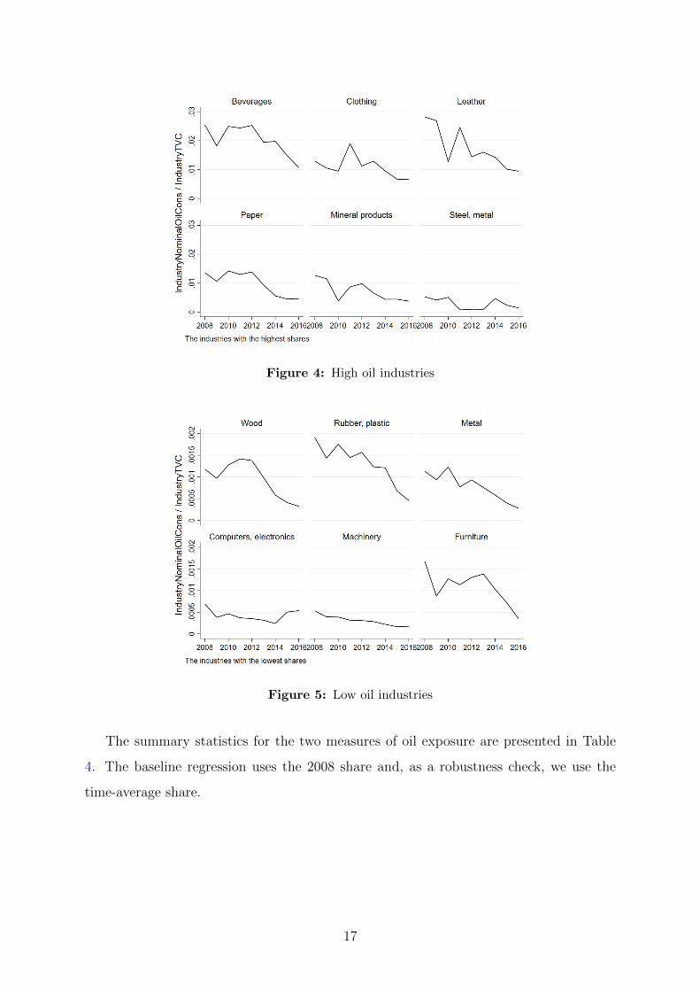
Figure 2 depicts the monthly Brent oil spot prices and returns.

Figure 2: Monthly Brent oil spot prices and returns

We consider a GARCH model of oil price volatility, assuming a stationary oil price

return series. The estimated GARCH(1,1) process is

roilt = µ+ ρroilt−1 + ϵt, where ϵt = σtzt, zt ∼ N(0, 1)

σ2t = ω + αϵ2t−1 + βσ2

t−1.

The conditional heteroskedasticity of oil prices in the estimated GARCH(1,1) model

of oil prices has both significant autoregressive and moving average components. The

GARCH(1,1) model can then be used to form expectations of the input price variance

over the next 12 month horizon for each time period.

14

The expected volatility is calculated as the expected standard deviation

(23) E[SDt] =

√√√√ 12∑i=1

Etσ2t+i,

which is the square root of the sum of the time t expectation of the Brent price variance

over the next 12 months.

By using an annual measure for the expected standard deviation, we implicitly assume

that firms set prices every year; and when they do, they consider volatility for the coming

year during which they will be stuck with the price they set. The annual expected

standard deviation is depicted in Figure 3.

Figure 3: Annual expected standard deviation

The summary statistics for the annual expected standard deviation is presented in

Table 2. The mean of expected volatility is 0.3 and its standard deviation is 0.02.

Table 2: Summary statistic: volatility

Mean SD p5 p50 p95

E[SDt] 0.31 0.02 0.30 0.30 0.36

15

3.5 Bartik shift-shares

The firm’s exposure to oil price volatility is measured by its industry’s nominal oil con-

sumption as a share of its industry’s total nominal variable costs. The regressions use the

variation in these industry-level variables. In particular, we compare the markup of firms

that are in industries with low oil exposures to the markup of firms that are in industries

with high oil exposure. The 24 manufacturing industries with their 2-digit industry codes

corresponding to the NACE (in Swedish SNI) classification are listed in Table 3. Table 3

includes statistics about the number of firms operating in the industry and the industries’

oil shares.

Table 3: List of 2-digit industries, number of firms and their oil shares

NACE Industry name Firms Ind2008Oil/TVC IndAvgOil/TVC

10 food products 823 0.0032 0.002211 beverages 27 0.0255 0.020313 textiles 116 0.0044 0.002714 wearing apparel 40 0.0129 0.011015 leather and related products 21 0.0282 0.017416 wood and of products of wood and cork, except furniture 644 0.0012 0.000917 paper and paper products 204 0.0136 0.009918 printing and reproduction of recorded media 395 0.0002 0.000119 coke and refined petroleum products 9 0.0022 0.001120 chemicals and chemical products 217 0.0026 0.002721 basic pharmaceutical products and pharmaceutical preparations 41 0.0056 0.005122 rubber and plastic products 430 0.0019 0.001323 other non-metallic mineral products 229 0.0127 0.007324 basic metals 208 0.0053 0.002925 fabricated metal products, except machinery and equipment 2029 0.0011 0.000826 computer, electronic and optical products 343 0.0007 0.000427 electrical equipment 269 0.0032 0.002128 machinery and equipment n.e.c. 903 0.0005 0.000329 motor vehicles, trailers and semi-trailers 101 0.0003 0.000230 other transport equipment 105 0.0025 0.001431 furniture 321 0.0017 0.001132 other manufacturing 199 0.0018 0.001133 repair and installation of machinery and equipment 442 0.0015 0.0011

Total number of firms 8116

Figure 4 shows the variation over time in the oil shares for industries with the highest

oil shares relative to the industry’s total variable cost. Figure 4 depicts the oil shares of

the industries with the lowest ratios.

16

Figure 4: High oil industries

Figure 5: Low oil industries

The summary statistics for the two measures of oil exposure are presented in Table

4. The baseline regression uses the 2008 share and, as a robustness check, we use the

time-average share.

17

Table 4: Summary statistics: exposures

Mean SD p5 p50 p95

Ind2008(Oil/TVC) 0.0025 0.0035 0.0003 0.0012 0.0127IndAvg(Oil/TVC) 0.0017 0.0024 0.0002 0.0009 0.0073

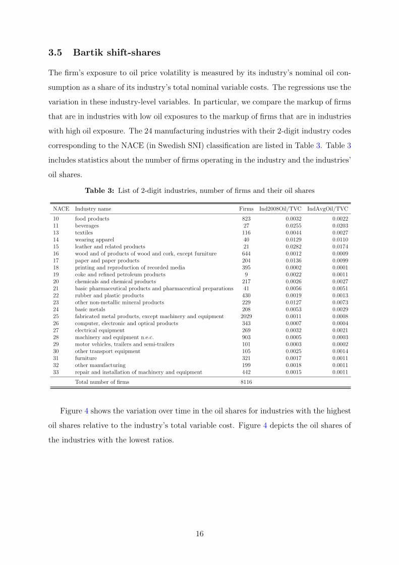
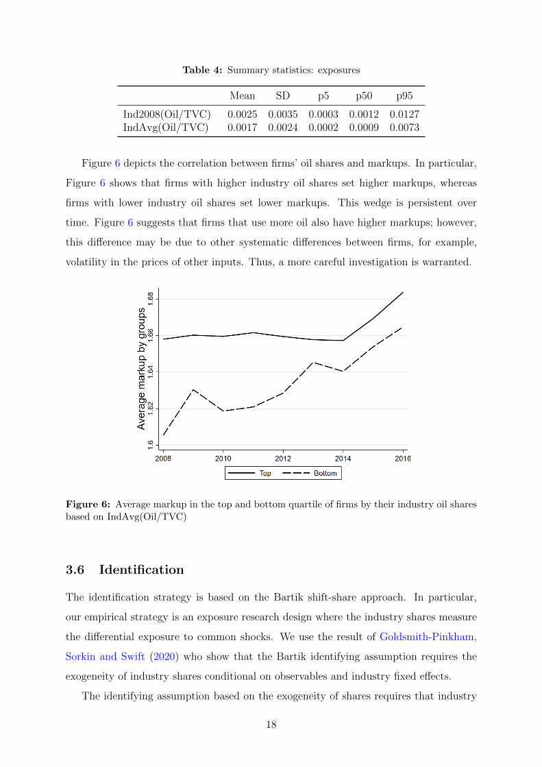
Figure 6 depicts the correlation between firms’ oil shares and markups. In particular,

Figure 6 shows that firms with higher industry oil shares set higher markups, whereas

firms with lower industry oil shares set lower markups. This wedge is persistent over

time. Figure 6 suggests that firms that use more oil also have higher markups; however,

this difference may be due to other systematic differences between firms, for example,

volatility in the prices of other inputs. Thus, a more careful investigation is warranted.

Figure 6: Average markup in the top and bottom quartile of firms by their industry oil sharesbased on IndAvg(Oil/TVC)

3.6 Identification

The identification strategy is based on the Bartik shift-share approach. In particular,

our empirical strategy is an exposure research design where the industry shares measure

the differential exposure to common shocks. We use the result of Goldsmith-Pinkham,

Sorkin and Swift (2020) who show that the Bartik identifying assumption requires the

exogeneity of industry shares conditional on observables and industry fixed effects.

The identifying assumption based on the exogeneity of shares requires that industry

18

oil shares are not correlated with confounding variables which may affect markups. The

exogeneity of shares assumption implies that a higher oil exposure of one industry as

compared to another is associated with a higher level of markup only because oil prices

are volatile and not because the shares are correlated with unobservables. The central

identification concern under the shares assumption is that the industry’s exposure to oil

may be correlated with demand or some other factor that affects the markup. In order

to address concerns about a plausible permanent relation between demand, markups and

oil shares, we include industry fixed effects as controls.

In addition, we fix industries’ oil share at their first year value in 2008. Using

time-invariant shares eliminates the possibility that industry-specific variation in demand

causes variation in markups through variation in industry oil shares. A remaining threat

to identification may be if the initial oil shares in 2008 are correlated with the variation

in demand and the variation in markups overtime. It is difficult to construct a plausible

scenario where this would occur because it would require a stochastic trend in industry

demand that is correlated with the industry oil shares in 2008.

We include year fixed effects in our estimation to control for unobserved confounding

variables that are correlated with the general business cycle. Year fixed effects account for

the average annual effect of the business cycle on markups. In particular, year fixed effects

eliminate the concern that oil price volatility and levels of oil prices may be correlated

with levels of demand and therefore affect markups.

In summary, our identifying assumption is that changes in demand that correlate with

oil price volatility do not differentially affect firms in industries with higher oil shares given

controls and the use of initial industry oil shares as exposure.

4 Results

Table 5 presents the main results. To interpret the coefficient in the first column in Table

5, we can multiply one standard deviation in volatility (0.02) with the average 2008

Oil/TVC ratio (0.0025) and the coefficient of 76.17. This estimate implies that a one

standard deviation increase in volatility leads to a 0.38 percent increase in the markup

of firms with average oil exposure. For example, a volatility increase from the average

0.31 to 0.33 leads to an increase in the average markup from 1.63 to 1.636. The effect is

19

stronger for firms with high oil exposure. A one standard deviation increase in volatility

leads to a 1.98 percent increase in the markup of firms with industry oil exposure in the

95th percentile versus only 0.05 percent for firms with industry oil exposure in the 5th

percentile.

Table 5: Main regression

(1) (2)lnmarkupCD lnmarkupTL

Ind2008(Oil/TVC) × E[SDt] 76.17∗∗∗ 81.87∗∗∗

(20.06) (22.60)Year FE X XIndustry FE X XObservations 46122 46122Adjusted R2 0.612 0.749

Notes: Standard errors are two-way clustered at the industry × yearlevel. Regressions are sales-weighted. Ind2008(Oil/TVC) is the two-digit industry’s oil to TVC ratio in 2008 and E[SDt] is expectedvolatility in year t given by equation (23). Stars +10% *5% **1%and ***0.1%.

Table 6 shows that the within-industry average percentage change in markups is about

4 percent, thus implying that about one tenth of the average within-industry variation

in markups is explained by this channel.

Table 6: Within industry summary statistics of markup changes

Mean SD p5 p50 p95|∆MarkupCDt| .0395846 .0325462 .0206375 .0306612 .0835094|∆MarkupCDt+1| .0502538 .029709 .0270304 .0404458 .112743|∆MarkupTLt| .0395846 .0325462 .0206375 .0306612 .0835094|∆MarkupTLt+1| .0502538 .029709 .0270304 .0404458 .112743

5 Robustness

5.1 Time-average industry exposure

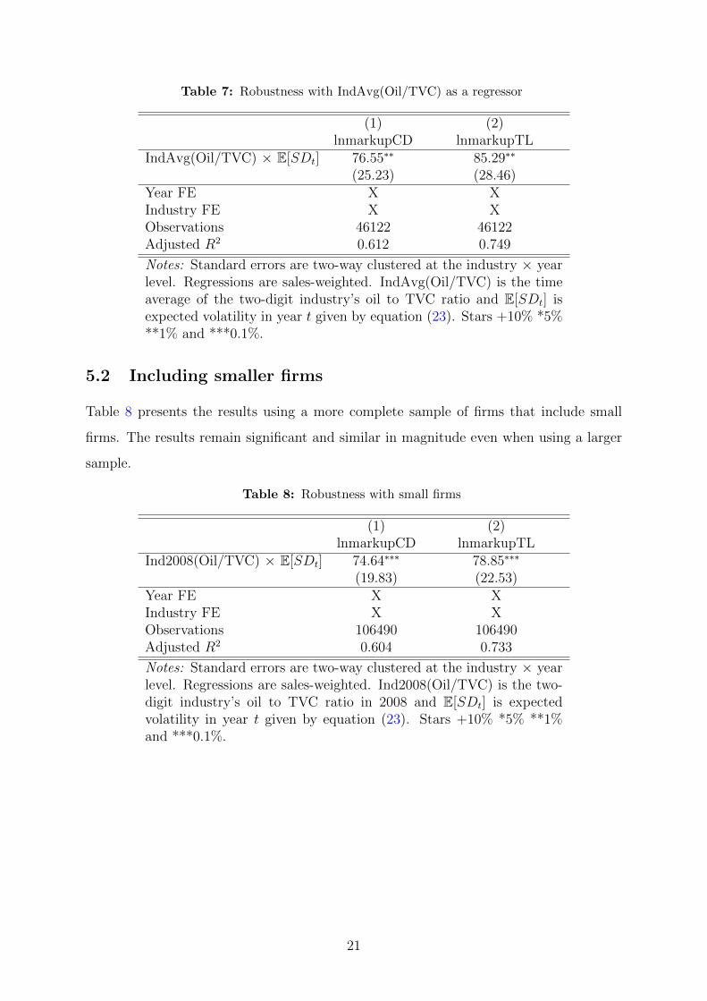
Table 7 presents the results using the time-average industry oil to TVC variable as ex-

posure. The results remain positive, significant and they are similar in magnitude.

20

Table 7: Robustness with IndAvg(Oil/TVC) as a regressor


IndAvg(Oil/TVC) × E[SDt] 76.55∗∗ 85.29∗∗


Notes: Standard errors are two-way clustered at the industry × yearlevel. Regressions are sales-weighted. IndAvg(Oil/TVC) is the timeaverage of the two-digit industry’s oil to TVC ratio and E[SDt] isexpected volatility in year t given by equation (23). Stars +10% *5%**1% and ***0.1%.

5.2 Including smaller firms

Table 8 presents the results using a more complete sample of firms that include small

firms. The results remain significant and similar in magnitude even when using a larger

sample.

Table 8: Robustness with small firms


Ind2008(Oil/TVC) × E[SDt] 74.64∗∗∗ 78.85∗∗∗



21

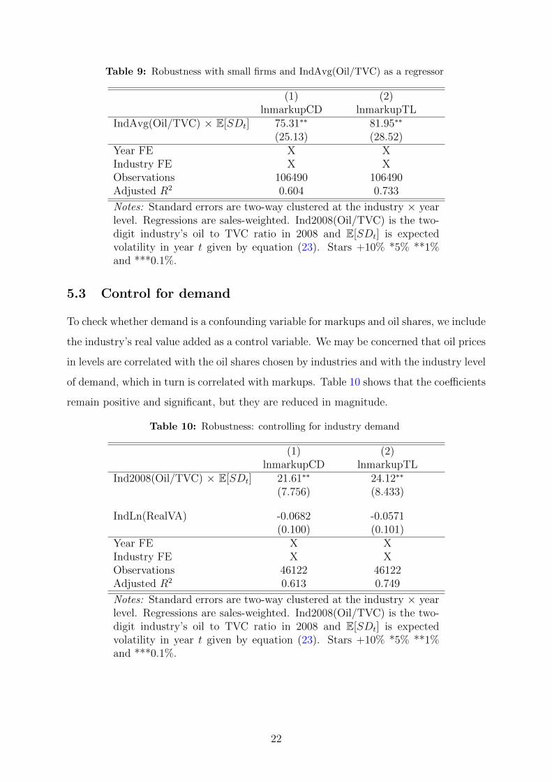
Table 9: Robustness with small firms and IndAvg(Oil/TVC) as a regressor


IndAvg(Oil/TVC) × E[SDt] 75.31∗∗ 81.95∗∗



5.3 Control for demand

To check whether demand is a confounding variable for markups and oil shares, we include

the industry’s real value added as a control variable. We may be concerned that oil prices

in levels are correlated with the oil shares chosen by industries and with the industry level

of demand, which in turn is correlated with markups. Table 10 shows that the coefficients

remain positive and significant, but they are reduced in magnitude.

Table 10: Robustness: controlling for industry demand


Ind2008(Oil/TVC) × E[SDt] 21.61∗∗ 24.12∗∗

(7.756) (8.433)

IndLn(RealVA) -0.0682 -0.0571(0.100) (0.101)

Year FE X XIndustry FE X XObservations 46122 46122Adjusted R2 0.613 0.749


22

5.4 Changes on changes regression

We try an additional estimation method using first differences in markups and volatility.

Table 11 depicts the coefficient estimates. The results confirm a positive relationship

but the magnitude is smaller. A standard deviation increase in volatility (0.02) increases

the markups by 0.04 percent for the firm with average oil exposure (0.002). Since the

within-industry average percentage change in markups is about 4 percent, this coefficient

estimate implies that only about one percent of the average variation in markups is

explained by this channel8

Table 11: First-difference regressions with Ind2008(Oil/TVC) as exposure

(1) (2) (3) (4)∆MarkupCDt ∆MarkupTLt ∆MarkupCDt+1 ∆MarkupTLt+1

Ind2008(Oil/TVC) × ∆E[SDt] 12.52∗∗∗ 12.22∗∗∗ -38.45 -42.23(3.499) (3.613) (24.06) (27.48)

Ind2008(Oil/TVC) × ∆P oilt 10.98 13.77 -119.2+ -123.3

(9.779) (10.50) (67.27) (76.79)

∆MarkupCDt−1,t−2 0.128 0.122+

(0.0863) (0.0733)

∆MarkupCDt−2,t−3 -0.111∗∗∗ -0.0916∗∗

(0.0318) (0.0304)

∆MarkupCDt,t−2 0.372∗∗∗ 0.427∗∗∗

(0.0499) (0.0600)

∆MarkupCDt−1,t−3 -0.183∗∗∗ -0.201∗∗∗

(0.0287) (0.0600)Observations 24140 24098 19060 18996Adjusted R2 0.112 0.074 0.249 0.251

Notes: Standard errors are two-way clustered at the industry × year level. Regressions aresales-weighted. All regressions control for year and industry fixed effects, as well as twolags of the dependent variable. Ind2008(Oil/TVC) is the two-digit industry’s oil to TVCratio in 2008 and ∆E[SDt] is the log change in the expected volatility from year t− 1 to t.∆MarkupCDt (∆MarkupCDt+1) is the log change in the markup between t (t+1) and t−1.Stars +10% *5% **1% and ***0.1%.

The summary statistics of markups, oil price and volatility changes are listed in Table

12. The averages refer to the means of variables in the full sample across firms and

industries.

8A potential reason for a small coefficient estimate may be due to the Nickel bias since the timeseries is relatively short and the first-difference regressions include lags as control variables to removethe potential serial correlation in the error term.

23

Table 12: Log changes in markups, oil prices and oil price volatility

mean sd p5 p50 p95∆MarkupCDt .0001531 .0633437 -.0627881 -.000414 .0671749∆MarkupCDt+1 .0024141 .0780057 -.078599 .0002822 .0910864∆MarkupTLt .0017258 .1426662 -.0814184 .0007474 .083904∆MarkupTLt+1 .0038752 .1741313 -.1067537 .0021562 .1144941∆E[SDt] .0021748 .0693593 -.1048869 -.0001293 .161683∆P oil

t .0756004 .0222737 .0304227 .084684 .0977478

6 Conclusion

In this paper, we study how uncertainty about factor prices leads to higher markups. Our

model predicts that the exposure of firms to the price volatility of major inputs matters

for the determination of firm-level markups. In particular, we find that firms with higher

shares of inputs with volatile prices in their total variable costs set higher markups.

We empirically test the implications of our model using the Bartik shift-share ap-

proach. We construct markups following the production function approach developed by

De Loecker and Warzynski (2012) and Ackerberg, Caves and Frazer (2015). We mea-

sure uncertainty in input prices by estimating the annual expected standard deviation of

monthly oil price changes within a simple GARCH model. The identifying assumption we

make in our estimation is that changes in demand that correlate with oil price volatility

do not differentially affect firms in industries with higher oil shares.

We show that a one standard deviation increase in volatility leads to a 0.38 percent

increase in the markup of firms with average oil exposure. The effect is stronger for firms

with high oil exposure. A one standard deviation increase in volatility leads to a 1.98

percent increase in the markup of firms with industry oil exposure in the 95th percentile

versus only 0.05 percent for firms with industry oil exposure in the 5th percentile.

The average within-industry change in markups is about 4 percent, suggesting that

our proposed channel explains one tenth of the average within-industry markup variation.

The effect is statistically and economically significant and thus, our findings help us

understand the variation in markups across firms and over time.

In terms of the economic significance, Gamber (2020) estimates large effects of markups

on revenue, ranging from 21.7% to 64.4%. His findings suggest that the business cycle

implications of even small changes in markups could be substantial. Future research may

24

find it interesting to explore the output and labor implications of variation in markups

due to input price volatility.

Our results also support the notion that firms are financially constrained and they

want to avoid situations with low profits. This is consistent with Gilchrist, Schoenle,

Sim and Zakrajsek (2017) and Lian and Ma (2020) who assume that firms are financially

constrained because they face an added cost when raising equity or issuing debt.

25

References

Abel, Andrew B., “Optimal Investment Under Uncertainty,” American Economic Re-

view, 1983, 73 (1), 228–233.

Ackerberg, Daniel A., Kevin Caves, and Garth Frazer, “Identification Properties

of Recent Production Function Estimators,” Econometrica, 2015, 83 (6), 2411–2451.

Bai, Yan, Patrick Kehoe, and Cristina Arellano, “Financial Markets and Fluc-

tuations in Uncertainty,” Meeting Papers 896, Society for Economic Dynamics, 2011,

(896).

Bloom, Nicholas, “The Impact of Uncertainty Shocks,” Econometrica, 2009, 77 (3),

623–685.

Born, Benjamin and Johannes Pfeifer, “Uncertainty-driven business cycles: Assess-

ing the markup channel,” Quantitative economics, 2021, 12 (2), 587–623.

Dixit, Avinash K. and Joseph E. Stiglitz, “Monopolistic Competition and Optimum

Product Diversity,” American Economic Review, 1977, 67 (3), 297–308.

Gamber, W., “Entry, Concentration, and Employment over the Business Cycle,” Work-

ing Paper, 2020.

Gilchrist, Simon, Raphael Schoenle, Jae Sim, and Egon Zakrajsek, “Inflation

Dynamics during the Financial Crisis,” American Economic Review, March 2017, 107

(3), 785–823.

Goldsmith-Pinkham, Paul, Isaac Sorkin, and Henry Swift, “Bartik Instruments:

What, When, Why, and How,” American Economic Review, 2020, 110 (8), 2586–2624.

Gutierrez, German and Thomas Philippon, “Declining Competition and Invest-

ment in the U.S.,” NBER Working Paper Seri, July 2017.

Hartman, Richard, “The effects of price and cost uncertainty on investment,” Journal

of Economic Theory, 1972, 5 (2), 258–266.

Karabarbounis, Loukas and Brent Neiman, “The global decline in the labor share,”

Quarterly Journal of Economics, 2014, 129 (1), 61–104.

26

and , “Accounting for Factorless Income,” NBER Working Paper Series, March

2018.

Klepacz, Matthew, “Price Setting and Volatility: Evidence from Oil Price Volatility

Shocks,” Working Paper, November 2020.

Levinsohn, James and Amil Petrin, “Estimating Production Functions Using Inputs

to Control for Unobservables,” The Review of Economic Studies, 2003, 70 (2), 317–341.

Lian, Chen and Yueran Ma, “Anatomy of Corporate Borrowing Constraints,” Quar-

terly Journal of Economics, 09 2020, 136 (1), 229–291.

Loecker, Jan D. De and Frederic Warzynski, “Markups and Firm-Level Export

Status,” American Economic Review, 2012, 102 (6), 2437–2471.

Loecker, Jan De, Jan Eeckhout, and Gabriel Unger, “The Rise of Market Power

and the Macroeconomic Implications,” Quarterly Journal of Economics, 01 2020, 135

(2), 561–644.

, Pinelopi K. Goldberg, Amit K. Khandelwal, and Nina Pavcnik, “Prices,

Markups, And Trade Reform,” Econometrica, 2016, 84 (2), 445–510.

Nakamura, Emi and Dawit Zerom, “Accounting for Incomplete Pass-Through,” The

Review of Economic Studies, 07 2010, 77 (3), 1192–1230.

Oi, Walter Y., “The Desirability of Price Instability Under Perfect Competition,”

Econometrica, 1961, 29 (1), 58–64.

Olley, G. S. and Ariel Pakes, “The Dynamics of Productivity in the Telecommunica-

tions Equipment Industry,” Econometrica, 1996, 64 (6), 1263–1297.

Rovigatti, Gabriele, “Markup estimation using Stata: Micro and Macro approaches

with markupest,” Working Paper, 2020.

and Vincenzo Mollisi, “Theory and Practice of Total-Factor Productivity Estima-

tion: The Control Function Approach using Stata,” The Stata Journal, 2018, 18 (3),

618–662.

SCB, “FEK Quality declaration 2017,” Statistics Sweden Documents, 2017.

27

A Appendix

A.1 Markups

Analytical definition of the firm markup Firm-level markups are constructed fol-

lowing De Loecker and Warzynski (2012) (DLW). The theoretical foundation for defining

markups is based on the cost minimization problem of a firm with one variable input,

labor Lit with associated wages wit. The Lagrangian function can be set up as

(24) Lit = witLit + ritKit + λit(Yit − Fit(Lit, Kit, ωit))

The first-order condition with respect to the single-variable input is

(25)∂Lit

∂Lit

= wit − λit∂Fit(Lit, Kit, ωit)

∂Lit

Since the marginal cost of production∂Lit

∂Yit

is λit, markups can be defined as the price-cost

margin µ ≡ Pit

λit

. Equating the first-order condition with zero and multiplying both sides

of it by Lit/Yit gives

(26)∂Fit(Lit, Kit, ωit)

∂Lit

Lit

Yit

=1

λit

witLit

Yit

which states that the output elasticity equals the inverse marginal cost times the labor

share of output. Using the definition of the markup and defining the output elasticity θit

as the left-hand side of equation (26) yields

(27) µit =θLitαLit

where θLit is the output elasticity and αLit is the labor share of output witLit

PitYit.

Estimation The estimation requires specifying the functional form for the production

function. Note that assuming a Cobb-Douglas production function for Fit introduces the

implicit assumption that output elasticities are common across all firms, i.e. θ ≡ βl in

28

the linear regression of

(28) yit = βllit + βkkit + ωit + ϵit

DLW uses the value-added translog production function as their baseline specification

which takes the form

(29) yit = βllit + βkkit + βlll2it + βkkk

2it + βlklitkit + ωit + ϵit.

The translog production function does not require the restrictive assumption of smooth

substitution between production factors and it is parsimonious in terms of the data re-

quirement. Assuming a translog production function yields firm-specific output elastici-

ties

(30) θLit = βl + 2βlllit + βlkkit

which can be computed directly using the estimated betas (β = βl, βk, βkl, βll, βkk).

To proxy for the unobserved productivity ωit, we use the control function method

proposed by Levinsohn and Petrin (2003) (LP). Specifically, we assume that changes in

material inputs (mit = ft(kit, lit, ωit)) are perfectly correlated with productivity shocks.

In practice, this assumption requires that firms adjust the level of intermediate inputs

immediately after the technical efficiency shock is realized. The LP control function

is corrected for functional dependence following Ackerberg et al. (2015) (ACF). ACF

prescribes a two-step procedure for estimating the production function. The first step

is to invert the intermediate input demand and express the unobserved productivity

ωit = f−1t (kit, lit,mit) as in LP and substitute it into the production function such that

the first stage (Cobb-Dougles production) becomes

(31) yit = β0 + βllit + βkkit + f−1t (kit, lit,mit) + εit = Φt(kit, lit,mit) + εit.

In the first stage, f−1t is estimated non-parametrically so that β = β0, βl, βk are not

identified separately but are estimated within the function Φt(kit, lit,mit) = β0 + βllit +

29

βkkit + ωit. The resulting first-stage moment condition is

(32) E[εit] = E[yit − Φt(kit, lit,mit)] = 0.

In this way, the correction of the functional dependence is achieved by conditioning on

labor within the estimation of the first stage. Since ACF cannot estimate βl in the first

stage (unline LP), βl is estimated along with the other production function parameters

in the second stage. To illustrate the exact moment conditions used in the second stage,

we use ACF’s example and define the functional form of the productivity process as an

AR(1) ωit = ρωit−1 + ξit. With this simple functional form assumption, the following

second-stage moment conditions are used for the estimation

(33) E

[(ωit(β)− ρωit−1(β))⊗

1

lit−1

kit

Φt−1(kit−1, lit−1,mit−1)

]= 0

which is equivalent to

(34)

E

[(yit−β0−βllit−βkkit−ρ(Φt−1−β0−βllit−1−βkkit−1))⊗

1

lit−1

kit


]= 0

or simply

(35) E

[ξit ⊗

1

lit−1

kit


]= 0

Since the second stage requires estimating an additional parameter βl as compared to

LP, an additional unconditional moment is required relative to LP. A natural set of four

second-stage moment conditions to estimate the three production function parameters in

β and ρ include the lagged value lit−1 in order to avoid that labor is chosen after time t-1

30

and is therefore correlated with the error term ξit.

Note that the actual estimation retains the OP/LP/ACF assumption of a general func-

tional form for the productivity process which evolves according to a first-order Markov

process according to

(36) ωit = E(ωit|ωit−1) + uit = g(ωit−1) + uit

where g(ωit−1) is left unspecified and approximated by an nth order polynomial. We use

a 4th order polynomial.

In addition, the estimation accounts for Olley and Pakes’ (1996) observation of the

inherent selection problem generated by the relationship between the unobserved pro-

ductivity variable and the exit decision of firms. Specifically, less productive firms find

it optimal to shut down, thus yielding selection into production. To be able to use an

unbalanced panel, we address attrition in the data by estimating g(ωit−1, χit) where χit

is an indicator function for the attrition in the market. The practical implementation of

the estimation follows Rovigatti and Mollisi (2018).

The final step in the markup estimation procedure is to use the first-stage residuals

in (31) to correct the labor share αlit. Since the observed output yit includes the error,

y∗it = yitexp(εit), it is possible to use the fitted residuals in (31) to obtain the corrected

markups as

(37) αl∗it =

witlitpit

yitexp(εit)

=witlitpity∗it

.

This completes the markup estimation procedure.

Implicit assumptions The assumption of common factor prices is the main assump-

tion underlying the DLW markup estimation based on OP/LP/ACF production func-

tions. Since the intermediate input demand equation mit = ft(kit, lit, ωit) is not indexed

by other factors, e.g. factor prices, it is assumed that these input prices are common

across firms. For this assumption to be reasonable, the production function - and the

elasticity of output derived from it - is estimated industry by industry in line with ACF

and DLW.

To estimate a real production function, which is a function that maps real inputs to

31

real output, all variables are deflated prior to the estimation. For the production function

estimation, log values are used in all variables and thus, negative and zero values are

eliminated in the process. All variables are annual. An itemized variable description

follows.

Capital The balance sheet value of the firm’s capital stock is defined as the firm’s

buildings, land, machines and intangible capital. The individual capital items are first

deflated using the appropriate 2-digit industry deflators, namely a deflator for buildings,

machines and intangible capital. Then, the deflated capital values are added together to

get the firm-level capital measure.

Labor Labor costs, including social contributions, are defined as the total wages in the

income statement of the firm. This variable is deflated by the wage index specific to the

industry where the firm operates.

Value Added Value added is the firm’s value added item calculated by the Swedish

Statistics agency for each firm. Value added is a measure of the total value added pro-

duced by the enterprise (that is, its contribution to the gross domestic product) and it

is defined in the Structural Business Statistics as the production value minus the cost of

purchased goods and services used as inputs in the production. This does not include

wages, social security contributions and the purchase cost of goods sold without process-

ing (SCB, 2017). This variable is deflated by the value added price index specific to the

industry where the firm operates.

Material Inputs Material inputs are the firm’s raw material inputs and the intermedi-

ate inputs in the firm’s income statement. The material inputs are calculated as the sum

of the two items and deflated by the 2-digit industry-specific intermediate input deflator.

Caveats of estimating translog markups with GMM Rovigatti (2020) uses simu-

lations to show that the Cobb-Douglas markups overlap with the baseline markups even

in the presence of measurement error, whereas translog markups are much less reliable to

deliver the baseline distribution when measurement error is present. In particular, mod-

erate and high measurement errors generate a bimodal distribution for translog markups,

32

with a noisy hump shaped tail on the right-end. The degenerate tail implies that the

estimated larger translog markups are more likely to be farther from their true value.

In addition, Rovigatti and Mollisi (2018) show that the ACF methodology has lim-

itations in empirical applications with translog markups due to the use of the GMM

optimizer. Rovigatti and Mollisi (2018) report the bias and MSE estimates with dif-

ferent starting points for the GMM optimization routine.9 Specifically, they show that

the coefficient estimates for the production elasticity are significantly different when the

optimizer’s starting points are fixed at the true values as compared to when the start-

ing points depart from the true values. The estimation error is increasingly worse for

extreme values of the starting point departures. Rovigatti and Mollisi (2018) note that

lower starting points lead to very noisy but not very biased results, while for larger val-

ues the bias increases and is statistically significant. This problem related to the starting

points is particularly pronounced for the translog production function since it requires a

selection of five starting points whereas the Cobb-Douglas production function requires

only two. This difficulty implies that translog markups within the tails of the translog

markup distribution are likely to be estimated with larger errors.

9Rovigatti and Mollisi (2018) use an optimization routine with the Newton–Raphson (NR) optimizeralgorithm that they deem to perform best across different optimizers.

33

Date post:	02-Jan-2022
Category:	Documents
Upload:	others
View:	3 times
Download:	0 times