MARKUPS, GAPS, AND THE WELFARE COSTS OF BUSINESSFLUCTUATIONS
Jordi Galı, Mark Gertler, and J. David Lopez-Salido*
Abstract—We present a simple theory-based measure of the variations inaggregate economic efficiency: the gap between the marginal product oflabor and the household’s consumption leisure tradeoff. We show that thisindicator corresponds to the reciprocal of the markup of price over socialmarginal cost, and give some evidence in support of this interpretation. Wethen show that, with some auxiliary assumptions, our gap variable may beused to measure the efficiency costs of business fluctuations. We find thatthe latter costs are modest on average. However, to the extent that theflexible price equilibrium is distorted, the gross efficiency losses fromrecessions and gains from booms may be large. Indeed, we find that themajor recessions involved large efficiency losses. These results hold forreasonable parameterizations of the Frisch elasticity of labor supply, therelative risk aversion, and steady-state distortions.
I. Introduction
TO the extent that there exist price and wage rigidities, orpossibly other types of market frictions, the business
cycle is likely to involve inefficient fluctuations in theallocation of resources. Specifically, the economy may os-cillate between expansionary periods when the volume ofeconomic activity is close to the social optimum, andrecessions that feature a significant drop in productionrelative to the first best. In this paper we explore thishypothesis by developing a simple measure of aggregateinefficiency and examining its cyclical properties. The mea-sure we propose—which we call the inefficiency gap, or thegap, for short—is based on the size of the wedge betweenthe marginal product of labor and the marginal rate ofsubstitution between consumption and leisure. Deviationsof this gap from 0 reflect an inefficient allocation of em-ployment. By constructing a time series measure of theinefficiency gap, we are able to obtain some insight intoboth the nature and the welfare costs of business cycles.
From a somewhat different perspective, we show that theinefficiency gap corresponds to the reciprocal of the markupof price over social marginal cost. Procyclical movements inthe inefficiency gap accordingly mirror countercyclicalmovements in this markup. Our approach, however, differsfrom much of the recent literature on business cycles andmarkups by using the household’s marginal rate of substi-tution between consumption and leisure to measure the
price of labor, as opposed to wages.1 As a matter of theory,of course, the household’s consumption leisure tradeoff isthe appropriate measure of the true social cost of labor.Wage data are not appropriate if either wages are notallocative or labor market frictions are present that drive awedge between market wages and the labor supply curve.As we demonstrate, our markup construct is highly coun-tercyclical. In addition, it also leads directly to a measure ofaggregate efficiency costs at each point in time.
Our approach builds on a stimulating paper by Hall(1997) that analyzes the cyclical behavior of the neoclassi-cal labor market equilibrium. Specifically, Hall first demon-strates that the business cycle is associated with highlyprocyclical movements in the difference between the ob-servable component of the household’s marginal rate ofsubstitution and the marginal product of labor. He thenpresents some evidence to suggest that this difference is ofcentral importance to employment fluctuations. Also rele-vant is Mulligan (2002), who examines essentially the samemeasure of the labor market wedge, though focusing on itslow-frequency movements. Specifically, he constructs anannual series of this variable, using data spanning more thana century. He finds that marginal tax rates correlate well atlow frequencies with this labor market wedge. Finally,Chari, Kehoe, and McGrattan (2004) find that the labormarket wedge plays a critical role in accounting for the dropin employment during the Great Depression.
As with Hall, we focus on the behavior of the labormarket wedge at the business cycle frequency. We differ inseveral important ways, however. First, his framework treatsthis wedge simply as an exogenous driving force, interpret-able, for example, as reflecting shifts in preferences.2 Weinstead stress countercyclical markup variations as the keyfactor accounting for the cyclical fluctuations in this vari-able and present evidence in support of this general hypoth-esis. Second, given our markup interpretation, we are ableto use the Hall residual as the basis for a measure of theefficiency costs of business cycles.
In particular, with some auxiliary assumptions, it is pos-sible to derive a measure of the lost surplus in the labormarket at each point in time, based directly on movements
Received for publication October 29, 2003. Revision accepted forpublication November 1, 2005.
* CREI and Universitat Pompeu Fabra, New York University, andFederal Reserve Board and CEPR, respectively.
We thank Jeff Amato, Susanto Basu, Bob Hall, Andy Levin, CaseyMulligan, Jonathan Parker, Julio Rotemberg, and several anonymousreferees for helpful comments, as well as participants in seminars at LSE,Bocconi, IIES, UPF, Bank of Spain, Bank of England, NBER SummerInstitute, CERGE, EUI, CEU, UAB, and the ECB Workshop on DSGEModels. Galı is thankful to CREA-Barcelona Economics, the Bank ofSpain, the MCYT, and DURSI for financial support. Gertler acknowledgesthe support of the NSF and the C. V. Starr Center. The opinions expressedhere are solely those of the authors and do not necessarily reflect the viewsof the Board of Governors of the Federal Reserve System or of anyoneelse associated with the Federal Reserve System.
1 See Rotemberg and Woodford (1999) for a survey of the literature onbusiness cycles and countercyclical markups.
2 To organize his approach, Hall (1997) modeled the labor marketresidual as an unobserved preference shock, though he did not take thishypothesis literally, but rather as a starting point for subsequent analysis.There has been a tendency in subsequent literature, however, (for exam-ple, Holland & Scott, 1998; Francis & Ramey, 2001; Uhlig, 2002) tointerpret this residual as an exogenous preference shock. Earlier literatureas well offered a similar interpretation (for example, Baxter & King,1991). Our analysis will suggest that this residual cannot simply reflectexogenous preference shifts.
in our gap variable. Fluctuations generate efficiency costson average because, as we show, the surplus lost from adecline in employment below its natural level exceeds thegain from a symmetric rise above its natural level. In thisrespect, our approach differs significantly from that ofLucas (1987, 2003), who examines the welfare costs ofconsumption variability associated with the cycle. Whereasthe Lucas measure does not really take account of thesources of fluctuations, our measure instead isolates thecosts associated with the inefficient component of fluctua-tions. Accordingly, our metric may give a better sense of thepotential gains from improved stabilization policy.
A significant additional feature is that our approach per-mits not only a measure of the costs of fluctuations onaverage, but also an assessment of the costs of particularepisodes. We find, for example, that although the efficiencycosts of fluctuations are not large when averaged acrossbooms and recessions, the gross gains from booms andlosses from recessions can indeed be quite large. Indeed, aswe show, our methodology suggests that the U.S. economyexperienced large efficiency costs during both the 1974–1975 and the 1980–1982 recession. This consideration ishighly relevant because it may be that the main benefit fromgood stabilization policies may be to avoid severe reces-sions. To the extent that central banks have had either goodskill or good luck in keeping to a minimum the number ofsevere downturns, it may be that on average the costs offluctuations are not large. This kind of unconditional calcu-lation, however, masks the kind of losses that can emerge ifluck and/or skill suddenly turn bad. For this reason, anexamination of episodes where matters clearly did seem togo awry can shed light on the importance of good policymanagement.
In section II we develop a framework for measuring theinefficiency gap in terms of observables, conditional onsome reasonably conventional assumptions about prefer-ences and technology. We also show that it is possible todecompose the gap into price and wage markup compo-nents. In section 3 we present empirical measures of thisvariable for the postwar U.S. economy. The inefficiency gapexhibits large procyclical swings. In addition, under theassumption that wages are allocational, most of its variationis associated with countercyclical movements in the wagemarkup.3 The price markup shows, at best, a weak contem-poraneous correlation. Under some alternatives to our base-line case, the price markup does move countercyclically.However, movements in the wage markup still dominate theoverall movements in the gap.
In section IV we consider the possibility that purelyexogenous factors (such as unobserved preference shifts)
underlie the variation in our gap measures. Specifically, wepresent evidence that suggests that our gap variable isendogenous and thus cannot simply reflect exogenous vari-ation in preferences. The evidence is instead consistent withour maintained hypothesis that endogenous variation inmarkups is largely responsible for the movement in theinefficiency gap. In section 5 we then use this link toexamine both the unconditional efficiency costs of reces-sions and the conditional costs associated with the majorboom-bust episodes. Concluding remarks are in section VI.
II. The Gap and Its Components: Theory
Let the inefficiency gap (henceforth, the gap) be definedas follows:
gapt � mrst � mpnt, (1)
where mrst and mpnt denote, respectively, the (log) marginalproduct of labor and the (log) marginal rate of substitutionbetween consumption and leisure.
As illustrated by figure 1, our gap variable can be repre-sented graphically as the vertical distance between theperfectly competitive labor supply and labor demand curves,evaluated at the current level of employment (or hours). Inmuch of what follows we assume that our gap variablefollows a stationary process with a (possibly nonzero)constant mean, denoted by gap (without any time subscript).The latter represents the steady-state deviation between mrst
and mpnt. Notice that these assumptions are consistent withboth mrst and mpnt being nonstationary, as is likely to be thecase in practice as well as in the equilibrium representationof a large class of dynamic business cycle models.
We next relate the gap to the markups in the goods andlabor markets. Under the assumption of wage-taking firms,and in the absence of labor adjustment costs, the nominalmarginal cost is given by wt � mpnt, where wt is (log)compensation per additional unit of labor input (includingnonwage costs). Accordingly, we define the aggregate pricemarkup as follows:
�tp � pt � �wt � mpnt� (2)
3 In this respect our results are consistent with recent evidence inSbordone (2000, 2002), Galı and Gertler (1999), Galı, Gertler and Lopez-Salido (2001), and Christiano, Eichenbaum, and Evans (1997, 1999, 2005)that in somewhat different contexts similarly points to an important rolefor wage rigidity.
FIGURE 1.—THE GAP: A DIAGRAMMATIC EXPOSITION
MARKUPS, GAPS, AND THE WELFARE COSTS OF BUSINESS FLUCTUATIONS 45
� mpnt � �wt � pt�. (3)
The aggregate wage markup is given by
�tw � �wt � pt� � mrst, (4)
that is, it corresponds to the difference between the wageand the marginal disutility of work, both expressed in termsof consumption. Notice that the wage markup should beunderstood in a broad sense, including the wedge created byefficiency wages, payroll taxes paid by the firm and laborincome taxes paid by the worker, search frictions, and so on.
A variety of frictions (perhaps most prominently, wageand price rigidities) may induce fluctuations in the markups:it is in this respect that these frictions are associated withinefficient cyclical fluctuations, or more precisely, withvariations in the aggregate level of (in)efficiency. In partic-ular, given that the marginal rate of substitution is likely tobe procyclical, rigidities in the real wage—resulting eitherfrom nominal or real rigidities—will give rise to counter-cyclical movements in the wage markup.4 Similar rigiditiesmay give rise, in turn, to a countercyclical price markup inresponse to demand shocks; for holding productivity con-stant, the marginal product of labor is countercyclical.5
Alternatively, procyclical movements in competitivenesscould induce a countercyclical price markup, as in Rotem-berg and Woodford (1996), for example.
To formalize the link between markup behavior and thegap, we first express equation (1) as
Combining equations (3), (4), and (5) then yields afundamental relation linking the gap to the wage and pricemarkups:
gapt � � ��tp � �t
w�. (6)
In the steady state, further,
gap � � ��p � �w� � 0, (7)
where variables without time subscripts denote steady-statevalues.
It is natural to assume that �tp � 0 and �t
w � 0 for all t,implying gapt � 0 for all t. In this case the level ofeconomic activity is inefficiently low (that is, the gap isalways negative), so that (small) increases in our gap mea-
sure will be associated with a smaller distortion (that is, anallocation closer to the perfectly competitive one). Noticealso that countercyclical movements in these markups implythat the gap is high in booms and low in recessions.
To the extent that we can measure the two markups (or, atleast their variation), we can characterize the behavior of thegap, as well as its composition. Constructing our gap vari-able requires some assumptions about technology and pref-erences. Below we consider a baseline case with reasonablyconventional assumptions. Decomposing the resulting gapvariable between wage and price markups requires an ad-ditional assumption, namely, that the observed wages usedin the construction of the markup reflect the shadow cost ofhiring an additional unit of labor. Because this assumption islikely to be more controversial, it is important to keep inmind that it is not necessary in order to measure the gap asa whole, but it is only used in computing its decompositionbetween the two markups.
Under the assumption of a technology with constantelasticity of output with respect to hours (say, ), we have(up to an additive constant):
mpnt � yt � nt, (8)
where yt is output per capita and nt is hours per capita.6
We assume that the (log) marginal rate of substitution fora representative consumer can be written (up to an additiveconstant) as
mrst � ct � �nt � �� t, (9)
where ct is consumption per capita and ��t is a low-frequencypreference shifter. The parameter rameter is related to thecoefficient of relative risk aversion, and � measures thecurvature of the disutility of labor.7 Following Hall (1997),we allow for the possibility of low-frequency shifts inpreferences over consumption versus leisure, as representedby movements in ��t. These preference shifts may be inter-preted broadly to include institutional or demographicchanges that affect the labor market, but which are unlikelyto be of relevance at business cycle frequencies. We differfrom Hall, though, by restricting these shifts to the lowfrequency. In section IV we provide evidence to justify thisassumption.
4 Models with countercyclical wage markups due to nominal rigiditiesinclude Blanchard and Kiyotaki (1987) and Erceg, Henderson, and Levin(2000). Alexopolous (2004) develops a model with a real rigidity due toefficiency wages that can generate a countercyclical wage markup. Alter-natively, Hall (1997) stresses the possible role of countercyclical searchfrictions to account for the behavior of the labor market residual.
5 With productivity shocks, the markup could be procyclical (becausethe marginal product of labor moves procyclically in that instance).
6 Under certain assumptions, that specification is compatible with vari-able labor utilization—particularly, if labor effort moves roughly propor-tionately with hours per worker, and the latter is highly positivelycorrelated with aggregate hours (per capita), as the evidence suggests. See,for example, Basu and Kimball (1997) for a detailed discussion.
7 The parameter � measures the curvature of the utility function underthe standard assumption that labor supply adjusts along the intensivemargin (that is, over hours). As we show in appendix A, however, undercertain assumptions our framework also allows for labor supply adjust-ment to occur instead over the extensive margin (that is, over participa-tion). Finally, this log linear representation of the mrs has been reconciledwith balanced growth in a model with household production (see Baxterand Jermann 1999), or in a generalized indivisible labor model (see Kingand Rebelo, 1999).
THE REVIEW OF ECONOMICS AND STATISTICS46
Under the above assumptions our gap variable is thusgiven by
gapt � � ct � � nt � �� t� � � yt � nt�. (10)
Furthermore, we can combine the above assumptions withthe definition of the price markup to obtain
�tp � � yt � nt� � �wt � pt� (11)
� � st. (12)
Hence the price markup can be measured (up to anadditive constant) as minus the (log) real unit labor costs,denoted by st. Similarly, the wage markup is given by
�tw � �wt � pt� � � ct � � nt� � �� t. (13)
III. The Gap and Its Components: Evidence
We now use the theoretical relations in the previoussection to construct measures of the gap and its two maincomponents: the price and wage markups. Our evidence isbased on quarterly postwar U.S. data over the sample period1960:I–2004:IV.8
A. Baseline Case
Identification of gap and wage markup variations requiresthat we make an assumption on the coefficient of relativerisk aversion and on �, a parameter that corresponds to theinverse of the (Frisch) wage elasticity of labor supply. A vastamount of evidence from microdata suggests a labor supplyelasticity mostly concentrated in the range of 0.05–0.5.9 Onthe other hand, the business cycle literature tends to usevalues of unity and higher, using balanced-growth consid-erations as a justification, as opposed to direct evidence(see, for example Cooley & Prescott, 1995). We use as abaseline value � 1, which we view as a reasonablecompromise between the values suggested in the micro andmacro literature. In addition, because it will turn out that thecosts of fluctuations vary inversely with the Frisch labor
supply elasticity, we are biasing our analysis against findinglarge welfare costs by choosing an elasticity that is abovemost of the direct estimates in the literature.
The efficiency costs are also increasing in the coefficientof relative risk aversion, because this parameter also affectsthe steepness of the labor supply curve. There is, however,a similar controversy over the value of this parameter,which equals the inverse intertemporal elasticity of substi-tution. Direct estimates of the latter tend to fall in the range0.1–0.3. This evidence suggests a value of that variesfrom 10 to 3.10 On the other hand, balanced-growth consid-erations lead the macro literature to a value of unity (again,see Cooley & Prescott, 1995). We will use unity as ourbaseline case, again opting to bias our parameterizationagainst finding large efficiency costs.
In addition, we need to make an assumption to identifythe low-frequency shifter ��t. Let �t
w�(wt � pt)�(ct�� nt)be the observable component of the wage markup (condi-tional on values for and �). It follows that
�tw � �t
w � �� t. (14)
From this perspective, the wage markup �tw is the “cyclical”
component of �tw, and ��t is (minus) the “trend” component.
We approximate the low-frequency movements of the wagemarkup by fitting a third-order polynomial of time to �t
w.11
Finally, before proceeding, we note that the relationshipsderived in the previous section hold only up to an additiveconstant. Accordingly, our framework allows us to identifythe variations over time in the markup and its components,but not their levels. Identification of the level requires thatwe calibrate the steady-state markup gap �(�p��w), anissue to which we turn below.
Our baseline results thus employ measures of the priceand wage markups and the gap constructed using, respec-tively, equations (6), (12), and (13), expressed in terms ofdeviations from their respective sample means.
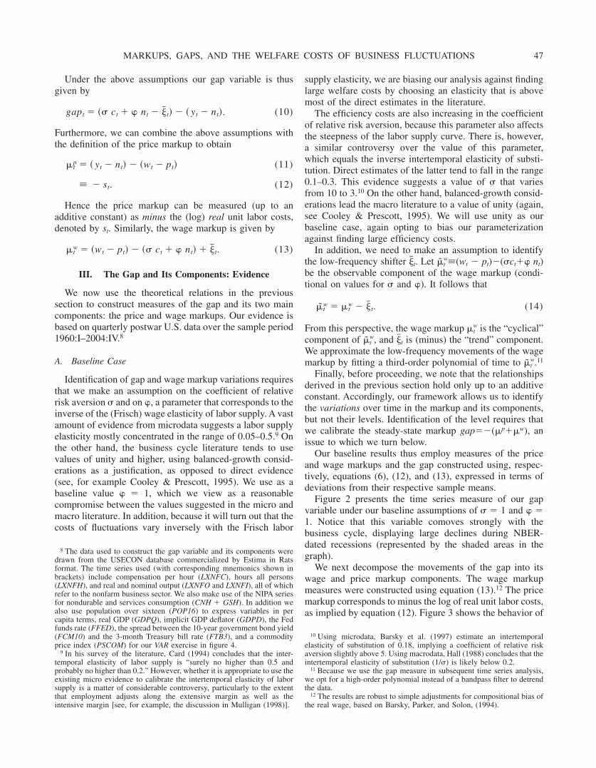
Figure 2 presents the time series measure of our gapvariable under our baseline assumptions of 1 and � 1. Notice that this variable comoves strongly with thebusiness cycle, displaying large declines during NBER-dated recessions (represented by the shaded areas in thegraph).
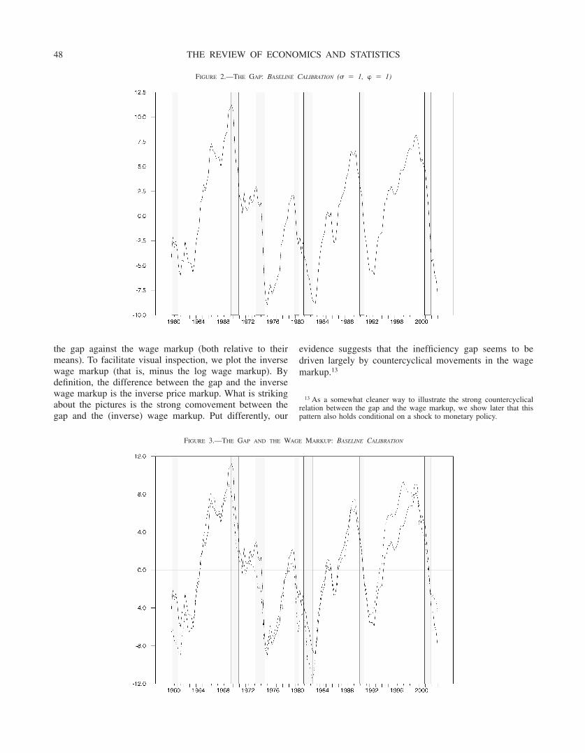
We next decompose the movements of the gap into itswage and price markup components. The wage markupmeasures were constructed using equation (13).12 The pricemarkup corresponds to minus the log of real unit labor costs,as implied by equation (12). Figure 3 shows the behavior of
8 The data used to construct the gap variable and its components weredrawn from the USECON database commercialized by Estima in Ratsformat. The time series used (with corresponding mnemonics shown inbrackets) include compensation per hour (LXNFC), hours all persons(LXNFH), and real and nominal output (LXNFO and LXNFI), all of whichrefer to the nonfarm business sector. We also make use of the NIPA seriesfor nondurable and services consumption (CNH � GSH). In addition wealso use population over sixteen (POP16) to express variables in percapita terms, real GDP (GDPQ), implicit GDP deflator (GDPD), the Fedfunds rate (FFED), the spread between the 10-year government bond yield(FCM10) and the 3-month Treasury bill rate (FTB3), and a commodityprice index (PSCOM) for our VAR exercise in figure 4.
9 In his survey of the literature, Card (1994) concludes that the inter-temporal elasticity of labor supply is “surely no higher than 0.5 andprobably no higher than 0.2.” However, whether it is appropriate to use theexisting micro evidence to calibrate the intertemporal elasticity of laborsupply is a matter of considerable controversy, particularly to the extentthat employment adjusts along the extensive margin as well as theintensive margin [see, for example, the discussion in Mulligan (1998)].
10 Using microdata, Barsky et al. (1997) estimate an intertemporalelasticity of substitution of 0.18, implying a coefficient of relative riskaversion slightly above 5. Using macrodata, Hall (1988) concludes that theintertemporal elasticity of substitution (1/) is likely below 0.2.
11 Because we use the gap measure in subsequent time series analysis,we opt for a high-order polynomial instead of a bandpass filter to detrendthe data.
12 The results are robust to simple adjustments for compositional bias ofthe real wage, based on Barsky, Parker, and Solon, (1994).
MARKUPS, GAPS, AND THE WELFARE COSTS OF BUSINESS FLUCTUATIONS 47
the gap against the wage markup (both relative to theirmeans). To facilitate visual inspection, we plot the inversewage markup (that is, minus the log wage markup). Bydefinition, the difference between the gap and the inversewage markup is the inverse price markup. What is strikingabout the pictures is the strong comovement between thegap and the (inverse) wage markup. Put differently, our
evidence suggests that the inefficiency gap seems to bedriven largely by countercyclical movements in the wagemarkup.13
13 As a somewhat cleaner way to illustrate the strong countercyclicalrelation between the gap and the wage markup, we show later that thispattern also holds conditional on a shock to monetary policy.
FIGURE 2.—THE GAP: BASELINE CALIBRATION ( 1, � 1)
FIGURE 3.—THE GAP AND THE WAGE MARKUP: BASELINE CALIBRATION
THE REVIEW OF ECONOMICS AND STATISTICS48
To be clear, our conclusion that countercyclical wagemarkup variation drives the variation in the gap rests on theassumption that wages are allocational and can thus be usedto construct a relevant cost measure.14 Though this assump-tion is standard in the literature on business cycles andmarkups (for example, Rotemberg & Woodford, 1999), it isnot without controversy. Notice, however, that even if ob-served wages are not allocational, our gap variable is stillappropriately measured, because its construction does notrequire the use of wage data. Thus our welfare analysis,which depends on the overall gap and not its decomposition,is not affected by this issue.
Table 1 reports some basic statistics that support thevisual evidence in figure 3. In particular, the table reports aset of second moments for the gap and its two components(the wage and price markups) and also for detrended (log)GDP, a common indicator of the business cycle. Note firstthat the percentage standard deviation of the gap is large(relative to detrended output) and that departures of the gapfrom steady state are highly persistent. In addition, the wagemarkup is nearly as volatile as the overall gap, and isstrongly negatively correlated with the latter, as well as withdetrended GDP. This confirms the visual evidence thatmovements in the gap are strongly associated with counter-cyclical movements in the wage markup. On the other hand,the price markup is less volatile than the wage markup anddoes not exhibit a strong contemporaneous correlation withthe gap.15
B. Robustness to Alternative Specifications of Technologyand Costs
We next investigate the robustness of our results to theuse of alternative specifications of technology and costs.Our baseline case assumes constant elasticity of output withrespect to hours and takes the observed average wage as therelevant cost of hiring additional labor. We consider fouralternatives to this baseline proposed by Rotemberg and
Woodford (1999) in their analysis of cyclical markup be-havior. The specific formulations and (subsequent calibra-tions) we use follow their analysis closely.
Each of the alternatives to the baseline enhances thecountercyclical movement in the price markup by makingmarginal cost more procyclical. The first alternative modelassumes a CES production function, thus relaxing the as-sumption of a constant elasticity of output with respect tolabor. The second model allows for overhead labor. Thethird model, which is based on Bils (1987), allows for themarginal wage to differ from the average wage due to anovertime premium. Finally, the fourth model allows forconvex costs of adjusting labor.
In appendix B we present a detailed exposition of howeach case affects the measure of the gap and its markupcomponents. We also discuss the calibration. As the appen-dix makes clear, the CES, overhead labor, and adjustmentcost models all alter the marginal product of labor. Theyaccordingly affect the measures of both the overall gap andthe price markup. However, they do not affect the measureof the wage markup. On the other hand, the marginal wagemodel alters only the composition of the gap between theprice and wage markups at each point in time, withoutinfluencing the gap variable itself (for it affects neither themarginal product of labor nor the household marginal rate ofsubstitution.)
The different panels of table 2 report basic statistics forthe alternative measures of the gap and its components,analogous to those reported in table 1 for the baseline case.Overall, the central results from our baseline case are robustto all the alternatives. Both the volatility and persistence ofthe gap are very similar across all cases. It also remains truein all cases that most of the variation in the gap is due to thevariation in the wage markup as opposed to the pricemarkup. The only significant difference is that the pricemarkup tends to display a stronger countercyclical move-ment than in the baseline case. In contrast to the baselinemodel, the price markup in the CES, overhead labor, andmarginal wage models is negatively correlated with theoutput gap. In all the alternative models, further, the nega-tive comovement of the price markup with our gap variableis larger than in the baseline case.
In panel A of figure 4 we show that the historical move-ment in the gap is robust to the alternative cases. We plotthe time series of the gap for the baseline case against all thealternatives except the marginal wage model (for which the
14 Some indirect evidence that wages are allocational is found bySbordone (2002) and Galı and Gertler (1999), who show that firms appearto adjust prices in response to measures of marginal cost based on wagedata. In turn, as shown in Galı (2001), they do not respond to marginal costmeasures that employ the household’s marginal rate of substitution inplace of the wage, as would be appropriate if wages were not allocational.
15 However, the relatively weak comovement of the price markup withdetrended output is useful for understanding the dynamics of inflation andthe recent evidence on the New Keynesian Phillips curve. See Sbordone(2002) and Galı and Gertler (1999).
Note: Column labeled GDP corresponds to the CBO output gap measure.
MARKUPS, GAPS, AND THE WELFARE COSTS OF BUSINESS FLUCTUATIONS 49
measure of the overall gap is the same as for the baseline).Clearly, the gap measures move very tightly together in allcases. Finally, though the gap measure in the marginalmodel is the same as in the baseline case, the division intoprice and wage markup movements differs. Accordingly, inpanel B of figure 4 we plot the wage markup for themarginal model (Bils adjustment) relative to the baselinecase. As the figure shows, the broad pattern in the move-ment of the wage markup is very similar across the twocases.
To summarize: the results thus far suggest that the busi-ness cycle is associated with large coincident movements inthe efficiency gap. Thus, under our framework, the evidencesuggests that countercyclical markup behavior is potentiallyan important feature of the business cycle. A decompositionof the gap further suggests that the countercyclical move-ment in the wage markup is by far the most importantsource of overall variations in the gap. Thus, to the extentthat wages are allocational, some form of wage rigidity,either real or nominal, may be central to business fluctua-tions.
IV. Labor Supply Shifts and the Gap
We have proceeded under the interpretation that ourmeasured gap between the marginal rate of substitution andthe marginal product of labor reflects countercyclicalmarkup behavior. In his baseline identification scheme,however, Hall modeled this gap as an unobserved prefer-ence shock, though he was clear to state that he did not takethis hypothesis literally. Subsequent literature, however (forexample, Holland & Scott, 1998; Francis & Ramey, 2001;Uhlig, 2002) has indeed interpreted this residual as reflect-ing either exogenous labor supply shifts or some otherunspecified exogenous driving force. In this section weshow that the high-frequency movements in the gap cannotbe simply due to exogenous preference shifts. Rather, theevidence is instead compatible with our countercyclicalmarkup interpretation.
Let us follow Hall (1997) in assuming that the marginalrate of substitution is now augmented with a preferenceshock �t that contains a cyclical component �t, as well as atrend component ��t:
mrst � ct � � nt � �t (15)
with
�t � �� t � �t,
where we maintain our baseline assumption that the coef-ficient of relative risk aversion, , is unity. Hall then definesthe residual xt as the difference between the “observable”component of the marginal rate of substitution, ct � � nt,and the marginal product of labor, yt�nt:
xt � �ct � � nt� � � yt � nt�. (16)
The issue then is how exactly to interpret the movementin Hall’s residual. Using the augmented specification (15) ofthe marginal rate of substitution allowing for preferenceshocks, together with equation (8) and the definition (1) ofthe inefficiency gap, it is possible to express xt as follows:
xt � �mrst � mpnt� � �t (17)
� � ��tp � �t
w� � �t. (18)
Hall’s assumption of perfect competition in both goodsand labor markets implies �t
p �tw 0. This allows him to
interpret the variable xt as a preference shock, for under thisassumption xt �t.16 Notice that under these circumstancesthe efficiency gap is 0, as there are no imperfections ineither goods or labor markets. On the other hand, if prefer-ences are not subject to shocks (�t 0, all t), and we allow
16 See also Baxter and King (1991). Holland and Scott (1998) constructsimilar measures for the United Kingdom.
TABLE 2.—BASIC STATISTICS: 1960–2004 — ROBUSTNESS: ALTERNATIVE MEASURES OF REAL MARGINAL COST
for departures from perfect competition, xt will purelyreflect movements in markups, that is, xt �(�t
p � �tw). In
the latter instance, xt corresponds exactly to our inefficiencygap, that is, xt gapt, for all t.
Note that if xt indeed reflects exogenous preferenceshocks, it should be invariant to any other type of distur-bance. In other words, the null hypothesis of preferenceshocks implies that xt should be exogenous. We next present
FIGURE 4.—(A) THE GAP: ALTERNATIVE MEASURES, BASELINE CALIBRATION ( 1, � 1), (B) WAGE MARKUP: BILS ADJUSTMENT
MARKUPS, GAPS, AND THE WELFARE COSTS OF BUSINESS FLUCTUATIONS 51
two tests that reject the null of exogeneity, thus rejecting thepreference shock hypothesis.
First, we test the hypothesis of no Granger causality froma number of variables to our gap measure. The variablesused are: detrended GDP, the nominal interest rate, and theyield spread. Both the nominal interest rate and the yieldspread may be thought of as rough measures of the stance ofmonetary policy, whereas detrended GDP is just a simplecyclical indicator. Table 3 displays the p-values for severalGranger-causality tests. These statistics correspond to biva-riate tests using alternative lag lengths. They indicate thatthe null of no Granger causality is rejected for all specifi-cations, at conventional significance levels. That finding isrobust to reasonable alternative calibrations of and �.Overall, the evidence of Granger causality is inconsistentwith the hypothesis that xt mainly reflects variations inpreferences.
As a second test, we estimate the dynamic response of ourgap variable to an identified exogenous monetary policyshock. The identification scheme is similar to the oneproposed by Christiano, Eichenbaum, and Evans (1999) andothers. It is based on a VAR that includes measures ofoutput, the price level, commodity prices, and the FederalReserve Funds rate, to which we add our gap measure (or,equivalently, Hall’s residual) and the price markup. Fromthe gap and the price markup response we can back out thebehavior of the wage markup, using equation (6). Weidentify the monetary policy shock as the orthogonalizedinnovation to the Federal Reserve Funds rate, under theassumption that this shock does not have a contemporane-ous effect on the other variables in the system.
Figure 5 shows the estimated responses to a contraction-ary monetary policy shock. The responses of the nominalrate, output, consumption, and prices are similar to thosefound in Christiano et al. (1999), Bernanke and Mihov(1998), and other papers in the literature. Most interestinglyfor our purposes, the inefficiency gap declines significantlyin response to the unanticipated monetary tightening. Itsoverall pattern of response closely mimics the response ofoutput. This endogenous reaction, of course, is inconsistentwith the preference shock hypothesis, but fully consistentwith our hypothesis that countercyclical markups may un-derlie the cyclical variation in the Hall residual. In thisconnection, note that the monetary shock induces a rise inthe wage markup that closely mirrors the decline in the gap,both in the shape and in the magnitude of the response. Thiscountercyclical movement in the wage markup is consistent
with evidence on unconditional comovements presented intable 1. The price markup also rises, though with a signif-icant lag. Apparently, the sluggish response of wages, whichgives rise to a strong countercyclical movement in the wagemarkup, delays the rise in the price markup.17 In any event,the decline in the inefficiency gap is clearly associated witha countercyclical rise in markups.
To be clear, because preference shocks are not observ-able, it is not possible to directly determine the overallimportance of these disturbances. Although our evidencerejects the hypothesis that exogenous preference variationdrives all the movement in our gap measure, it cannot ruleout the possibility that some of this movement is due topreference shocks. Yet, to the extent that preference shocksare mainly a low-frequency phenomenon, they are likely tobe captured by the trend component associated with ourlow-frequency filter (together with other institutional anddemographic factors which may lead to low-frequency vari-ations in markups). In this instance our filtered gap series,which isolates the high-frequency movement in this vari-able, is likely to be largely uncontaminated by exogenouspreference variations.
V. Welfare and the Gap
We next propose a simple way to measure the welfarecosts of fluctuations in the degree of inefficiency of aggre-gate resource allocations, as captured by our gap variable.We then apply this methodology to postwar U.S. data. Inaddition to obtaining a measure of the average cost of gapfluctuations, we also compute the welfare losses duringparticular episodes, including the major postwar recessions.
As we noted in the introduction, our approach differsfrom Lucas (1987) and others in focusing on the costsstemming from fluctuations in the degree of inefficiency ofthe aggregate resource allocation, as reflected by the move-ments in our gap variable.18 As in Ball and Romer (1987),the cycle generates losses on average within our framework
17 As Galı and Gertler (1999) and Sbordone (2002) observe, the sluggishbehavior of the price markup helps explain the inertial behavior ofinflation, manifested in this case by the delayed and weak response ofinflation to the monetary shock. Staggered pricing models relate inflationto an expected discounted stream of real marginal costs, which corre-sponds to the reciprocal of the price markup. The sluggish response to theprice markup translates into sluggish behavior of real marginal cost.
18 For other approaches to measuring the unconditional costs of fluctu-ations see, for example, Barlevy (2004) and Beaudry and Pages (2001).For a very early attempt to measure the welfare cost of inefficiently highunemployment, see Gordon (1973).
Note: The values reported are p-values for the null hypothesis of no Granger causality from each variable listed to Hall x (F-test). Filtered data using third-order polynomial in time.
THE REVIEW OF ECONOMICS AND STATISTICS52
because the welfare effects of employment fluctuationsabout the steady state are asymmetric. As figure 1 illustrates,given that the steady-state level of employment is inefficient(due to positive price and wage markups in the steady state),the efficiency costs of an employment contraction below thesteady state will exceed the benefits of a symmetric in-crease. In particular, note that the vertical distance betweenthe labor demand and supply curves rises as employmentfalls below the steady state, and falls as it rises above. Thequantitative effect of this nonlinearity on the welfare cost offluctuations ultimately depends on the slopes of the labordemand and supply curves, and on the steady-state distancerelative to the first-best, perfectly competitive steady state.
Underlying this measure of the average costs of fluctua-tions are the gross gains from booms and losses fromrecessions. As we elaborate, under our maintained hypoth-esis that the flexible price equilibrium is distorted (due toimperfect competition and taxes, and so on), there aresignificant first-order welfare losses from employment con-tractions below the steady state, as well as gains frommovements above. Below we present a time series measureof these gross efficiency costs and benefits, along with anoverall net measure.
A. A Welfare Measure
We now proceed to derive our welfare measure. Theeconomy is assumed to fluctuate around an underlying“frictionless” path characterized by a constant gap level:
GAP � MRSt
MPNt
� exp� � �� � 1 � � � 1,
where upper bars denote values along a constant gap path,and � is (minus) the steady-state value of our (log) gapvariable. A second-order approximation of the period utilityaround its level along the underlying constant-gap pathyields
�t � U�Ct,Nt� � U� �Ct, �Nt�
� �Uc,t �Ct� ct �1 �
2ct
2� � �Un,t �Nt� nt �1 � �
2nt
2� ,
where the tildes denote log deviations from the underlyingconstant-gap path, that is, xt � log�Xt/Xt�, and where � �� � �Unn,t
�Nt�/ �Un,t and � � �Ucc,t�Ct/ �Uc,t.
FIGURE 5.—DYNAMIC EFFECTS OF MONETARY POLICY SHOCKS: BASELINE CALIBRATION, SAMPLE PERIOD 1960–2004
Note: 95% confidence bands for impulse responses are based on 5000 Monte Carlo replications. Sample period: 1960:1–2004:3.
MARKUPS, GAPS, AND THE WELFARE COSTS OF BUSINESS FLUCTUATIONS 53
In order to maintain tractability, we make two additionalassumptions. First, we assume that all output is consumed,which in turn implies ct yt for all t. Secondly, we assumethat output is linearly related to hours in equilibrium, that is,yt at � nt, thus implying nt yt. The latter assumption isconsistent with the notion that variations in the stock ofcapital are negligible at business cycle frequencies, and thatthe rate of capital utilization is proportional to hours. Noticethat these two assumptions imply that
��Un,t �Nt
U�c,t �Ct
� 1 � �.
Hence, we can rewrite the second-order approximation as
�t � �Uc,t �Ct��yt �1
2�� � �� � �1 � ���1 � ���yt
2�.
(19)
Furthermore, under the previous assumptions, togetherwith the log linear specification for the marginal rate ofsubstitution in equation (9), it is easy to check that
gapt � � � ��yt,
where gapt�gapt�gap. Using the previous expression tosubstitute for yt in equation (19), we obtain
�t
U�c,tC� t
�1
� ���gapt � �gapt
2�(20)
� �� gapt�
where � � 12�1 �
�1 � ���1 � ��
� � �.
Notice that ��gapt� is the period efficiency loss or gainfrom the gap’s deviations from its steady-state value, ex-pressed as a percentage of the frictionless level of consump-tion C� t. The first term in the parentheses, the linear term,reflects the symmetric first-order costs and benefits from thegap moving below and above the steady state, due to thepositive steady-state markup � (implying � � 0). Thequadratic term captures the asymmetric, second-order ef-fects of gap fluctuations on welfare. For plausible values of�, , and � we have � � 0. In that case � is concave,implying that a reduction in the gap below its steady-statevalue results in an efficiency loss that exceeds the gainstemming from a commensurate increase in the gap aboveits steady state.
We can use equation (20) to calculate a time series of theefficiency gain or loss in each quarter t. To obtain a measureof the average welfare cost over time analogous to thosefound in the literature, we take the unconditional expecta-tion of equation (20) to obtain
E� �t
U�c,t �Ct� � �
�
� �var�gapt�, (21)
where var(gapt) is the variance of our gap measure. Noticethat, as a result of the concavity of �, the expected welfareeffects of fluctuations in the gap variable are negative, thatis, these fluctuations imply losses in expected welfare. Thisloss, further, is of second order, as it is linearly related to thevariance of the inefficiency gap. It is, however, potentiallylarge, depending in particular on the magnitude var(gapt).As section 3 suggests, var(gapt) is potentially large if thelabor supply is inelastic or the risk aversion is high.
To be clear, our approach provides a lower bound on themeasure of the total welfare costs of fluctuations. Thereason is simple: it does not include the welfare costs fromefficient fluctuations in consumption and employment. Sup-pose, for example, that the data were generated by a real-business-cycle model with frictionless, perfectly competi-tive markets. We should then expect to see no variation inour gap measure, as the resource allocation would always beefficient. Our metric would then indicate no welfare costs offluctuations, but some losses would still be implied by thevariability of consumption and leisure (under standard con-vexity assumptions on preferences). It is also important tostress that, to the extent that the steady-state value of the gapcorresponds also to the average value around which theeconomy fluctuates (as assumed above), average welfarelosses will only be of second order. On the other hand, ourefficiency cost measure suggests possible first-order effectsat any moment in time: As reflected in equation (20) andillustrated further below, deviations in the gap variable fromthat steady state may have nonnegligible first-order welfareeffects, with the gap declines associated with recessionsgenerating large welfare losses.
B. Some Numbers
Equation (20) provides a real-time measure of the effi-ciency costs of deviations of our gap variable from steadystate. Accordingly, we construct a quarterly time series of��gapt�, taking as input our measure of the gap. We considerthree different parameterizations: first, our baseline casewith 1 and � 1; second, a case where we raise therisk aversion with 5 and � 1; and third, a case wherewe reduce the labor supply elasticity with 1 and � 5(implying a Frisch labor supply elasticity of 0.2). For theparameter �, the sum of the steady-state wage and pricemarkups, we assume a value of 0.50. A value of 0.15 to 0.20is plausible for the steady-state price markup (see Rotem-berg and Woodford, 1999). Inasmuch as the steady-statewage markup depends on tax distortions as well as workers’market power, 0.30 to 0.35 seems a reasonable lower boundgiven the evidence on average labor tax rates. This range isalso roughly consistent with the evidence in Mulligan(2002).
THE REVIEW OF ECONOMICS AND STATISTICS54
Figure 6 plots the resulting time series over the sample1960:4–2004:4. The value at each period t can be inter-preted as the efficiency gain or loss in percentage units of
consumption associated with the deviation of the ineffi-ciency gap from its steady state. Our baseline parametriza-tion indicates substantial fluctuations in welfare resulting
FIGURE 6.—THE WELFARE EFFECTS OF POSTWAR U.S. FLUCTUATIONS
MARKUPS, GAPS, AND THE WELFARE COSTS OF BUSINESS FLUCTUATIONS 55
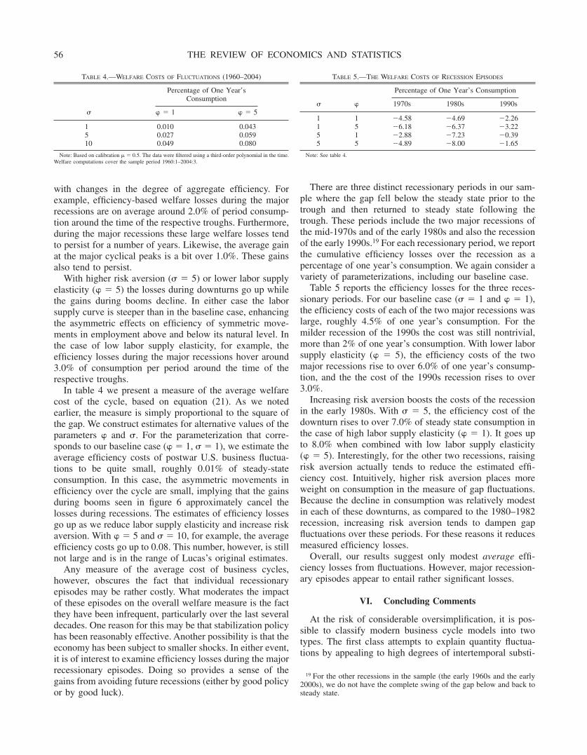
with changes in the degree of aggregate efficiency. Forexample, efficiency-based welfare losses during the majorrecessions are on average around 2.0% of period consump-tion around the time of the respective troughs. Furthermore,during the major recessions these large welfare losses tendto persist for a number of years. Likewise, the average gainat the major cyclical peaks is a bit over 1.0%. These gainsalso tend to persist.
With higher risk aversion ( 5) or lower labor supplyelasticity (� 5) the losses during downturns go up whilethe gains during booms decline. In either case the laborsupply curve is steeper than in the baseline case, enhancingthe asymmetric effects on efficiency of symmetric move-ments in employment above and below its natural level. Inthe case of low labor supply elasticity, for example, theefficiency losses during the major recessions hover around3.0% of consumption per period around the time of therespective troughs.
In table 4 we present a measure of the average welfarecost of the cycle, based on equation (21). As we notedearlier, the measure is simply proportional to the square ofthe gap. We construct estimates for alternative values of theparameters � and . For the parameterization that corre-sponds to our baseline case (� 1, 1), we estimate theaverage efficiency costs of postwar U.S. business fluctua-tions to be quite small, roughly 0.01% of steady-stateconsumption. In this case, the asymmetric movements inefficiency over the cycle are small, implying that the gainsduring booms seen in figure 6 approximately cancel thelosses during recessions. The estimates of efficiency lossesgo up as we reduce labor supply elasticity and increase riskaversion. With � 5 and 10, for example, the averageefficiency costs go up to 0.08. This number, however, is stillnot large and is in the range of Lucas’s original estimates.
Any measure of the average cost of business cycles,however, obscures the fact that individual recessionaryepisodes may be rather costly. What moderates the impactof these episodes on the overall welfare measure is the factthey have been infrequent, particularly over the last severaldecades. One reason for this may be that stabilization policyhas been reasonably effective. Another possibility is that theeconomy has been subject to smaller shocks. In either event,it is of interest to examine efficiency losses during the majorrecessionary episodes. Doing so provides a sense of thegains from avoiding future recessions (either by good policyor by good luck).
There are three distinct recessionary periods in our sam-ple where the gap fell below the steady state prior to thetrough and then returned to steady state following thetrough. These periods include the two major recessions ofthe mid-1970s and of the early 1980s and also the recessionof the early 1990s.19 For each recessionary period, we reportthe cumulative efficiency losses over the recession as apercentage of one year’s consumption. We again consider avariety of parameterizations, including our baseline case.
Table 5 reports the efficiency losses for the three reces-sionary periods. For our baseline case ( 1 and � 1),the efficiency costs of each of the two major recessions waslarge, roughly 4.5% of one year’s consumption. For themilder recession of the 1990s the cost was still nontrivial,more than 2% of one year’s consumption. With lower laborsupply elasticity (� 5), the efficiency costs of the twomajor recessions rise to over 6.0% of one year’s consump-tion, and the the cost of the 1990s recession rises to over3.0%.
Increasing risk aversion boosts the costs of the recessionin the early 1980s. With 5, the efficiency cost of thedownturn rises to over 7.0% of steady state consumption inthe case of high labor supply elasticity (� 1). It goes upto 8.0% when combined with low labor supply elasticity(� 5). Interestingly, for the other two recessions, raisingrisk aversion actually tends to reduce the estimated effi-ciency cost. Intuitively, higher risk aversion places moreweight on consumption in the measure of gap fluctuations.Because the decline in consumption was relatively modestin each of these downturns, as compared to the 1980–1982recession, increasing risk aversion tends to dampen gapfluctuations over these periods. For these reasons it reducesmeasured efficiency losses.
Overall, our results suggest only modest average effi-ciency losses from fluctuations. However, major recession-ary episodes appear to entail rather significant losses.
VI. Concluding Comments
At the risk of considerable oversimplification, it is pos-sible to classify modern business cycle models into twotypes. The first class attempts to explain quantity fluctua-tions by appealing to high degrees of intertemporal substi-
19 For the other recessions in the sample (the early 1960s and the early2000s), we do not have the complete swing of the gap below and back tosteady state.
TABLE 4.—WELFARE COSTS OF FLUCTUATIONS (1960–2004)
Percentage of One Year’sConsumption
� 1 � 5
1 0.010 0.0435 0.027 0.05910 0.049 0.080
Note: Based on calibration � 0.5. The data were filtered using a third-order polynomial in the time.Welfare computations cover the sample period 1960:1–2004:3.
tution in an environment of frictionless markets. The secondinstead appeals to countercyclical markups owing to partic-ular market frictions. In this regard, there has been aconsiderable debate as to whether the markup is indeedcountercyclical [see Rotemberg and Woodford (1999) for asummary]. Much of this debate has been centered aroundprice markup measures that use wage data to calculate thecost of labor. We show, however, that the markup is highlycountercyclical, using the household’s consumption leisuretradeoff as the shadow cost of labor, as theory wouldsuggest. Under this identification scheme, the markup cor-responds exactly to the labor market residual studied byHall (1997) and others. Whether the countercyclical markupvariation is driven primarily by product market or labormarket behavior is, however, an open question. To theextent that wages are allocative, we find that labor marketfrictions are the key factor. As we discussed, however, theexact form that these frictions may take (such as nominalwage rigidity, efficiency wages, or search frictions) is alsoan open question.
A second message of this paper is that to the extent thatour markup interpretation of the efficiency gap is correct,business cycles may involve significant efficiency costs. Tobe sure, our results suggest that these efficiency losses aremodest when averaged over time. This result occurs, how-ever, because—whether by good luck or good policy—significant recessions have not often occurred since WorldWar II. We find, however that when they do occur, theefficiency costs may indeed be quite large. These resultsobtain for reasonably standard assumptions on preferences(for example, a coefficient of relative risk aversion of 5 anda unit-elasticity Frisch labor supply). Thus, though the gainsfrom eliminating all fluctuations may not be large—assuggested by the existing literature—there nonetheless doappear to be significant efficiency benefits from avoidingsevere recessions.
Finally, we observe that our calculation ignores at leastseveral important considerations that might be leading us tounderstate the efficiency costs of recessions. First, withinour framework, a reduction in hours leads to increasedenjoyment of leisure, which partially offsets the impact ofthe output decline. In reality, workers who are laid offduring recessions do not simply get to enjoy the time off,but rather have to look for a new job. In addition, there isoften a loss of human capital that was specific to theprevious employer. Second, our calculation ignores thecosts of fluctuations in price and wage inflation associatedwith variations in markups resulting from nominal rigidities(see, for example, Woodford, 1999). For this reason, ourmetric may overstate the gains from booms (and understatethe losses from recessions). To the extent that the costs ofhigh inflation roughly offset the efficiency gains from theboom, our measure of the gross efficiency loss of therecession may provide a more accurate indicator of the costs
of these episodes. Taking these considerations into accountis on the agenda for future research.
REFERENCES
Alexopolous, Michelle, “Unemployment and the Business Cycle,” Jour-nal of Monetary Economics 51 (2004), 277–298.
Ball, Lawrence, and David Romer, “Are Prices Too Sticky?” QuarterlyJournal of Economics 104 (1987), 507–524.
Barlevy, Gadi, “The Cost of Business Cycles under Endogenous Growth,”American Economic Review 94:4 (2004), 964–990.
Barsky, Robert, Jonathon Parker, and Gary Solon, “Measuring the Cycli-cality of Real Wages: How Important is Composition Bias?”Quarterly Journal of Economics 109 (1994), 1–25.
Barsky, Robert, F. Thomas Juster, Miles S. Kimball, and Matthew D.Shapiro, “Preference Parameters and Behavioral Heterogeneity: AnExperimental Approach in the Health and Retirement Study,”Quarterly Journal of Economics 112 (1997), 537–579.
Basu, S., and M. Kimball, “Cyclical Productivity with Unobserved InputVariation,” NBER working paper no. 5915 (1997).
Baxter, M., and Robert King, “Productive Externalities and BusinessCycles,” Federal Reserve Bank of Minneapolis, Institute for Em-pirical Macroeconomics, discussion paper no. 53 (1991).
Baxter, M., and U. J. Jermann, “Household Production and the Excess ofSensitivity of Consumption to Current Income,” American Eco-nomic Review 89:4 (1999), 902–920.
Beaudry, Paul, and Carmen Pages, “The Cost of Business Cycles and theStabilization Value of Unemployment Insurance,” European Eco-nomic Review 45:8 (2001), 1545–1572.
Bernanke, Ben, and Ilyan Mihov, “Measuring Monetary Policy,” Quar-terly Journal of Economics 113 (1998), 869–902.
Blanchard Olivier, J., and Nobuhiro Kiyotaki, “Monopolistic Competitionand the Effects of Aggregate Demand,” American Economic Re-view 77 (1987), 647–666.
Card, David, “Intertemporal Labor Supply: An Assessment” (pp. 49–78),in Christopher Sims (Ed.), Advances in Econometrics: Sixth WorldCongress, Vol. II, (Cambridge University Press, 1994).
Chari, V. V., Kehoe, P., and Ellen R. McGrattan, “Business CyclesAccounting,” Federal Reserve Bank of Minneapolis staff report328 (2004).
Christiano, Lawrence, Martin Eichenbaum, and Charles Evans, “StickyPrices and Limited Participation Models: A Comparison,” Euro-pean Economic Review 41 (1997), 1201–1249.“Monetary Policy Shocks: What Have We Learned and to WhatEnd?” in J. Taylor and M. Woodford (Eds.), Handbook of Macro-economics, Vol. 1A (Amsterdam: North-Holland, 1999).“Nominal Rigidities and the Dynamic Effects of a Shock toMonetary Policy,” Journal of Political Economy 113:1 (2005),1–45.
Cooley, Thomas, and Edward Prescott, “Economic Growth and BusinessCycles,” in Thomas Cooley (Ed.), Frontiers of Business CycleResearch (Princeton University Press, 1995).
Eichenbaum, Martin, Lars Hansen, and Kenneth Singleton, “A TimeSeries Analysis of Representative Agent Models of Consumptionand Leisure Choice under Uncertainty,” Quarterly Journal ofEconomics 103:1 (1988), 51–78.
Erceg C., Dale Henderson, and Andrew Levin, “Optimal Monetary Policywith Staggered Wage and Price Contracts,” Journal of MonetaryEconomics 46:2 (2000), 281–313.
Francis, Neville, and Valerie Ramey, “Is the Technology-Driven Hypoth-esis Dead? Shocks and Aggregate Fluctuations Revisited,” UCSDmimeograph (2001).
Galı, Jordi, “The Case for Price Stability. A Comment,” in A. Garcia-Herrero, V. Gaspar, L. Hoogduin, J. Morgan, and B. Winkler (Eds.),Why Price Stability? (Frankfurt am Main, European Central Bank,2001).
Galı, J., and Mark Gertler, “Inflation Dynamics: A Structural EconometricAnalysis,” Journal of Monetary Economics 44 (1999), 195–222.
Galı, J., Mark Gertler, and J. David Lopez-Salido, “European InflationDynamics,” European Economic Review 45:7 (2001), 1121–1150.“Markups, Gaps, and the Welfare Costs of Business Fluctuations,”NBER working paper no. 8850 (2002).
Gordon, Robert J., “The Welfare Cost of Higher Unemployment,” Brook-ings Papers on Economic Activity 4:1 (1973), 133–195.
MARKUPS, GAPS, AND THE WELFARE COSTS OF BUSINESS FLUCTUATIONS 57
Hall, Robert E., “Intertemporal Substitution in Consumption,” Journal ofPolitical Economy 96:2 (1988), 339–357.“Macroeconomic Fluctuations and the Allocation of Time,” Jour-
nal of Labor Economics 15:1, pt. 2 (1997), S223–S250.Holland, A., and A. Scott, “Determinants of U.K. Business Cycles,”
Economic Journal 108 (1998), 1067–1092.King, Robert, and Sergio Rebelo, “Resuscitating Real Business Cycles,”
in J. Taylor and M. Woodford (Eds.), The Handbook of Macroeco-nomics, Vol. 1B (Amsterdam North-Holland, 1999).
Lucas, Robert E. Models of Business Cycles (Oxford University Press,1987).“Macroeconomic Priorities,” American Economic Review 93:1
(2003), 1–14.Mulligan, Casey B., “Substitution over Time: Another Look at Life-Cycle
Labor Supply,” in Ben Bernanke and Julio Rotemberg (Eds.),NBER Macroeconomics Annual, Vol. 13 (Cambridge, MA: MITPress, 1998).“A Century of Labor-Leisure Distortions,” NBER working paperno. 8774 (2002).
Pencavel, John, “The Market Work Behavior and Wages of Women,1975–94,” Journal of Human Resources 33 (1998), 771–804.
Rotemberg, Julio, and Michael Woodford, “The Cyclical Behavior ofPrices and Costs,” in J. Taylor and M. Woodford (Eds.), TheHandbook of Macroeconomics, Vol. 1B (Amsterdam: North-Holland, 1999).
Sbordone, Argia M. “An Optimizing Model of Wage and Price Dynam-ics,” Rutgers University mimeograph (2000).“Prices and Unit Labor Costs: Testing Models of Pricing Behav-ior,” Journal of Monetary Economics 45:2 (2002), 265–292.
Uhlig, Harald, “What Moves Real GNP?” presented at CEPR-ESSIMConference, May Tarragona, Spain (2002).
Woodford, M., “Inflation Stabilization and Welfare,” NBER workingpaper no. 5684 (1999).
APPENDIX A
The Household’s MRS
Here we illustrate that the expression we use for the household’smarginal rate of substitution between consumption and leisure, equation(9), may be motivated either by making the standard assumption that laborsupply adjusts along the intensive margin or, under certain assumptions,that the adjustment is along the extensive margin. Our argument is basedon Mulligan (1998).
Case I. Labor Supply Adjustment along the Intensive Margin: Let Ctand Nt denote consumption and hours worked, respectively. Assume arepresentative agent with preferences given by
1
1 � Ct
1 � �1
1 � �Nt
1 � �.
It follows that
MRSt � CtNt
�.
By taking the log of each side of this relation we obtain equation (9).
Case II. Labor Supply Adjustment along the Extensive Margin: Nowassume that individuals either do not work or work a fixed amount ofhours per week. Suppose there is a representative household with acontinuum of members represented by the unit interval, and who differaccording to their disutility of work. Specifically, let us assume that j� isthe disutility of work for member j. Under perfect consumption insurancewithin the household, and interpreting Nt as the fraction of workinghousehold members in period t, total household utility will be given by
1
1 � Ct
1 � � �0
Nt
j� dj.
Note that
�0
Nt
j� dj �1
1 � �Nt
1 � �
Accordingly, the utility function for the family in this case is isomor-phic to the case of adjustment along the intensive margin. It follows thatthe marginal rate of substitution has the same form as well.
APPENDIX B
Alternative Specifications
We now present the details that underlie the alternative measures of thegap and its components that we examined in the text. Our baseline caseassumes constant elasticity of output with respect to hours and takes theobserved average wage as the relevant cost of hiring additional labor. Thefour alternatives we consider are those proposed by Rotemberg andWoodford (1999) in their analysis of cyclical markup behavior. Asdiscussed in the text, deviations from the baseline include: CES produc-tion, overhead labor, marginal wage differing from the average wage dueto an overtime premium, and convex costs of adjusting labor.
As will become clear, the CES, overhead labor, and adjustment costmodels all alter the marginal product of labor. They accordingly affect themeasures of both the overall gap and the price markup, but not the wagemarkup. On the other hand, the marginal wage model alters only thecomposition of the gap between the price and wage markups at each pointin time, without influencing the gap variable itself.
1. Baseline Specification
Our baseline case assumes no adjustment costs and a productionfunction isoelastic in labor, that is, Yt F(Xt)Nt
. In this case we have thefollowing expressions for the (log) marginal product of labor and the pricemarkup (up to an additive constant):
mpnt � yt � nt,
�tp � pt � �wt � mpnt�
� � st,
where st is the log labor share. These two formulas are then used inconjunction with information on the households’ marginal rate of substi-tution to obtain measures of the gap and the wage markup.
2. CES Technology
Here we assume a CES production function: Yt � ��1 � �Kt1�1/�
� �ZtNt�1�1/�� �/���1�. The implied elasticity of output with respect to
labor input, �t � �Yt/�Nt/Nt/Yt, is given by
�t � 1 � �1 � �� Yt
Kt���1�1/��
.
Log-linearizing around a steady state yields (ignoring constants) log�t �(yt � kt), where � � (1 � ��1)(��1 � 1). Because MPNt
�tYt/Nt, we can write
mpnt � � yt � nt� � �� yt � kt�
and
�tp � pt�(wt�mpnt)
� � st � �� yt � kt�.
Calibration of � proceeds by first noticing that the gross price markup Mtp
equals MPNt/�Wt/pt�. This allows allows us to derive a simple expressionfor the steady state value of the elasticity of output with respect to laboras a function of the steady state price markup and the labor share, that is,
THE REVIEW OF ECONOMICS AND STATISTICS58
� SMp. Rotemberg and Woodford (1999) calibrate the coefficient �using approximate values for the average labor income share (S 0.7),the average gross price markup (close to unity), and an estimate forelasticity of substitution between capital and labor (� 0.5), all of whichcombined yield a value � �0.4.
3. Overhead Labor
For this case we assume a technology given by the production functionYt ZtKt
1 � (Nt �Nt*), where Nt* denotes the amount of overhead laborat each point in time. The elasticity of output with respect to (total) laborinput is now given by
�t � � Nt
Nt � Nt*� .
Log-linearizing around the steady state and ignoring constants yieldslog �t ��nt, where � � N*/N � N* is the steady-state ratio ofoverhead to variable labor, and nt denotes the log deviation of hours fromits long-run trend (around which the linearization is carried out). Using thefact that MPNt �tYt/Nt, it follows that
mpnt � yt � nt � �nt
and
�tp � pt � �wt � mpnt�
� � st � �nt.
Rotemberg and Woodford (1999) use a zero-profit condition in steadystate in order to calibrate �. In particular, it can be shown that the ratio ofaverage costs to marginal costs can be written as
ACt
MCt� 1 � � Nt*
Nt � Nt*� .
This implies the following steady-state relationship:
AC �1
M�
�
1 � �S.
Following Rotemberg and Woodford (1999), we assume S 0.7, M 1.25, and impose the zero-profit condition AC 1, thus implying � 0.4.We use the latter value to construct our overhead-labor measure of the gapand the price markup.
4. Marginal Wage Different from Average Wage
In the previous analysis we have assumed that firms are wage-taking,so that the marginal wage is equal to the average wage. As emphasized byBils (1987), this will not be the case if the wage rises as firms ask theiremployees to work more hours. The relevant wage needed to computeboth the price and wage markups is no longer the average wage but themarginal wage, Wm. Notice however, that the use of the marginal wagewill only alter the decomposition of our gap measure between the priceand the wage markup, but not the gap measure itself.
Let qt � wtm � wt denote the ratio of the marginal to the average wage
(expressed in logs). Then it follows that
�tp � pt � �wt
m � mpnt�
� pt � �wt � mpnt� � qt
� � st � qt.
Similarly,
�tw � �wt
m � pt� � mrst
� �wt � pt� � mrst � qt.
Bils (1987) and Rotemberg and Woodford (1999) propose a simplemodel of overtime pay that implies that the ratio Qt is an increasingfunction of hours per worker Ht. Log-linearization of that function arounda steady-state value for hours per worker allows us to rewrite the pricemarkup as
�tp � pt � �wt � mpnt� � �ht,
where � is the elasticity of the marginal-to-average wage ratio with respectto hours per worker.
Similarly, the wage markup will now be given by
�tw � �wt � pt� � mrst � �ht.
As discussed in Bils (1987), the assumption of a 50% overtimepremium (the statutory premium in the United States) implies � 1.4,which we use to construct our overtime measure of the price and wagemarkups.
5. Labor Adjustment Costs
Finally, we consider the implications of having a cost of adjustinglabor, which we assume take the form of output lost. Those cost are to betaken into account when computing firms’ marginal costs and hence pricemarkups. Following Rotemberg and Woodford (1999), we assume thatthose costs take the form UtNt�(Nt/Nt � 1), where Ut is the price of the inputrequired to make the adjustment. In this case, the (expected) total costassociated with hiring an additional worker for one period is given by
Wt�1 �Ut
Wt��� Nt
Nt � 1� �
Nt
Nt � 1��� Nt
Nt � 1�
� Et�Rt,t � 1
Ut � 1
Ut�Nt � 1
Nt� 2���Nt � 1
Nt���� � WtBt,
where Rt,t�1 is the usual stochastic discount factor for one-period-aheadincome.
Hence, the expression for the price markup is given by
�tp � pt � �wt � bt � mpnt�
� � st � bt.
Assuming that the ratio Ut/Wt is stationary, we can derive the followingexpression in terms of deviations from steady state as follows (ignoringconstants):
bt � ���nt � �Et��nt � 1��,
where � � (U/W)��(1) and � R u with u being the steady-state valuefor Ut�1/Ut. Hence, the expression for the price markup can now be writtenas
�tp � � st � ���nt � �Et��nt � 1��.
We construct our adjustment-cost measure of price markups under theassumption that � 0.99 and � 4, the values suggested by Rotembergand Woodford (1999).
MARKUPS, GAPS, AND THE WELFARE COSTS OF BUSINESS FLUCTUATIONS 59