Marriage and Money: The Impact of Marriage on Men’s and Women’s Earnings ** Belinda Hewitt*, Mark Western* and Janeen Baxter* Negotiating the Life Course Discussion Paper Series Discussion Paper DP- 007 July 2002 * Sociology, School of Social Science, The University of Queensland Email authors: [email protected]Paper prepared for the Australian Sociological Conference, Brisbane, 2002 ** This research was supported by funding from the Research School of Social Sciences (RSSS), The Australian National University. We would also like to thank members of the Negotiating the Lifecourse project for comments on an earlier version of this paper.
Transcript
Marriage and Money: The Impact of Marriage on Men’s and Women’s
Earnings **
Belinda Hewitt*, Mark Western* and Janeen Baxter*
Negotiating the Life Course Discussion Paper Series Discussion Paper DP- 007
July 2002
* Sociology, School of Social Science, The University of Queensland Email authors: [email protected] Paper prepared for the Australian Sociological Conference, Brisbane, 2002 ** This research was supported by funding from the Research School of Social Sciences (RSSS), The Australian National University. We would also like to thank members of the Negotiating the Lifecourse project for comments on an earlier version of this paper.
1991; Loh 1996; Schoeni 1995). There is, however, no consensus on whether role
specialisation or selection effects contribute to married men’s higher earnings.
Overall, marriage premium research finds support for both arguments, although on
balance there is stronger empirical support for the role specialisation productivity
thesis.
Korenman & Neumark (1991), using data from the National Longitudinal
Study of Young Men 1976 to 1980, and adjusting for comprehensive human capital
factors, found evidence that married men’s wages grew faster than single men’s, and
that this wage growth accounted for the majority of the marriage premium. They also
found that 80 per cent of the marriage premium remained after controlling for marital
selection. Korenman & Neumark (1991), conclude that their findings support the role
specialisation thesis because more of the premium appears to be attributable to factors
associated with the marriage institution rather than factors inherent in the men per se.
Ginther & Zavodny (2000) in their examination of the marriage premium used
shotgun weddings (defined as weddings that are followed by the birth of a child
within 7 months) as a natural experiment to control for selection into marriage, rather
than the more commonly used longitudinal fixed effects modelling. They argue that
shot gun weddings do not follow the same selection processes as other marriages and
therefore marital status and earnings ability may not be correlated in these marriages.
They examined data from the National Longitudinal Survey of Young Men and the
1980 Census 5% Public Use Microdata Sample, and found 90 per cent of the marriage
premium remained after controlling for selection into marriage (in addition to a range
of human capital characteristics).
In contrast, Loh (1996), using cross sectional data from the 1990 National
Longitudinal Survey of Youth Labor Market Experience examined the marriage
premium adjusting for effects of wives education and participation in the work force
on married men’s wages, in addition to controlling for human capital, job and family
characteristics. Loh found that the size of the premium did not change according to
the length of time (years) that married men’s wives had been in paid employment.
This finding throws doubt on the role specialisation theory since men with working
wives should benefit less from role specialisation within the household. Loh (1996)
concludes that it is unlikely that role specialisation productivity differences explain
the gap between married and unmarried men’s wages.
Interestingly it has been found in some studies that the marriage premium for
men is diminishing over time. Blackburn and Korenman (1994) describe a 10 per cent
decrease in the marriage premium over the 1970s. Similarly, Gray (1997), using 1976
to 1980 data from the National Longitudinal Survey and 1989 to 1993 data from the
National Longitudinal Survey of Youth, finds a decline of 40 per cent in the marriage
premium during the 1980s. In his study Gray used longitudinal data and independent
variables (ie respondents attitudes and values towards family and work) to control for
the selection of high earnings men into marriage, and included a control for the
number of hours worked by married men’s wives to test the specialisation hypotheses.
While he found selection and specialisation effects on men’s wages, he also
concluded that the decrease in the premium was primarily due to lower returns to
specialisation within marriage, because of the increasing participation of wives in the
labor force (Gray 1997: 500).
Implicit in both the role-specialisation and selection explanations for the
premium is the idea that the benefits from marriage are larger for men at the top of the
earnings distribution than those at the lower end. This is because men with high
earnings have either received greater gains from specialisation within marriage, or are
a more attractive spouse (Daniel 1995). In contrast to earlier research we do not
explicitly attempt to explain the existence of the premium, rather we use robust and
quantile regression models to achieve stable estimates of its size at different points on
the earnings distribution (the conditional mean and deciles). All previous research
focuses solely on the mean and thus it is not clear whether the impact of marriage is
constant or variable the further we move away from the mean.
Marriage and Women’s Earnings
Early research examining the determinants of women’s earnings found that marriage
had little or no association once adjustments were made for human capital (education,
work experience, tenure), job characteristics (hours worked, occupation, employment
conditions), and family status (the presence or number of children). For example, Hill
(1979) using data from the 1976 Panel Study of Income Dynamics found no
significant association between marriage and wages. Controlling for education, work
experience and number of children, her results show that married, white women earn
more than unmarried women, but less than divorced, separated or widowed women.
Dolton and Makepeace (1987) also found no association between marriage and wages
among female college graduates. Goldin and Polachek (1987), on the other hand,
using 1980 U.S. Census data found that single women had a wage advantage over
married women, but these differences were small once adjustments were made for
variability in expected levels of accumulated human capital.
More recent investigations have focused specifically on the wage penalty for
motherhood. Budig and England (2000) used the National Longitudinal Survey for
Youth, 1982-1993, and adjusting for a wide range of human capital, family, and job
characteristics, found a marriage premium for women of around 4 per cent. They also
found that being divorced, separated, and widowed had a larger effect on women’s
earnings than being married or never married. Their results also showed an interaction
effect between marriage and children, with the size of the marriage premium declining
as the number of children in the household increased so that by three children, there is
actually a wage penalty for motherhood (Budig & England 2000). Waldfogel (1997)
also found a marriage premium for women, but found that divorced, separated and
widowed women had higher earnings than both married and never married women.
Taken together this evidence suggests that the relationship between marriage
and women’s earnings appears to be changing. While earlier research found little, or
no, association between marriage and earnings, recent studies have found significant
positive associations. There are two possible explanations for this shift. First, there
have been major social changes for women since the 1970s, such as increased
participation in higher education and employment, which may have led to a shift in
the determinants of female earnings. On the other hand the observed change in the
relationship between marriage and wages for women could be attributable to
differences in statistical methods. Korenman and Neumark (1992) criticized the use of
cross-sectional techniques in examining the relationships between marriage,
motherhood and wages for women for underestimating the effects of these
determinants on wages. One consistent finding across all studies, however, is that
where there is a wage premium for marriage, women who are divorced, separated, and
widowed usually have higher wages than married women.
In summary, recent research finds a marriage premium for women, and
diminishing returns to marriage for married men. These findings possibly reflect long-
term effects of changes in women’s participation in higher education and the work
force, and changes in the nature of marriage. In this paper we examine the relationship
between marriage and earnings using cross-sectional data from a nationally
representative 1996/97 Australian study titled Negotiating the Life Course. First we
examine the nature and extent of the effects of marriage on earnings, emphasising
differences both between the sexes, and between individuals according to marital
status. Second we extend previous research by investigating the relationship between
marriage and earnings at different points on the conditional distribution, rather than
simply focusing on the mean. This latter issue has not been explored elsewhere in the
earnings literature.
Methods
Data
The data used in this paper come from a 1996/97 national Australian survey titled
“Negotiating the Life Course: Gender, Mobility and Career Trajectories” (NLC)
(McDonald et al 2000). The sample comprised 2,231 respondents between the ages of
18 and 54 randomly selected from listed telephone numbers in the electronic white
pages. Each respondent was randomly selected from all 18 to 54 year olds in the
household. The data were collected using computer assisted telephone interviewing
(CATI), with a response rate of 55%.
Sample
For the current analyses we restrict the sample to men and women who were
employed at the time of survey. Respondents who were on paid maternity or ‘other’
leave, such as sick or long service leave, are included. The self-employed are
excluded. There were 1299 respondents in the final sample.
Variables
The dependent and independent variables are described in Table 1. The dependent
variable is the natural log of gross (i.e. before tax) annual income. The primary
independent variable, marital status, consists of a series of dummy variables for never
married, previously married (divorced, separated, and widowed) and currently
married or cohabiting 1, with never married as the reference group. We follow
conventional practice for semi-logarithmic equations in interpreting the dummy
variable coefficients as indicating the percentage increment (premium) or decrement
(penalty) on earnings for the group coded 1 on the dummy variable in comparison to
the dummy variable reference category (see Wooldridge 2002: 43-47).
Table 1: Description of variables
Variables Definition of Variable Dependent: Annual Earnings (logged) Gross annual income, logged Primary Independent: Married Dummy variable for people in married or defacto relationships
(1=Married, defacto) Ever Married Dummy variable for people who were previously married
(1=Divorced, Separated or Widowed) Never Married Dummy for people who have never been married (Reference Category) Human Capital: Age Age of respondent Age#2 Age of respondent centred and squared to adjust for non-linear
relationship with wages Years of Education Continuous measure of years of education of respondent, incorporates
level of education measure and retrospective data from age of 15 years, retrospective component includes years of full-time and part-time study weighted by 0.5.
Degree or better Dummy for if respondent has bachelor degree or higher (1=Bachelor degree)
Years Work Experience Continuous measure of years of work experience, includes full-time years of work, and part-time years of work weighted by 0.5. Residualized with age so work experience is net of the influence of age.
Years Work Experience#2 Yrs Work Experience residualized, centred and squared. Family Status: Pre-school child Dummy for the presence of a preschool aged child in house
(1=preschool child present) No Children Dummy for No children in Household (Reference Group) One Child Dummy for One child in Household (1=1 Child) Two Children Dummy for Two children in Household (1=2 Children) Three, or more Children Dummy for Three or more children in Household
(1=3 or more Children) Job Characteristics: Government Sector Dummy for Government or Private sector (1=Government) Managerial Occupation (Reference group) Professional Occupation Dummy for professional occupation (1=Professional, associate
professional) White Collar Occupation Dummy for White collar employee (1=Sales, Service, Clerical) Blue Collar Occupation Dummy for Blue Collar employee (1=Trades, Labourer)
Human capital is measured by variables for age, education and work
experience. We use controls for age in years and age centred and squared (i.e. we
mean deviate age and then square this quantity). This captures the curvilinear effect of
age on earnings in cross-sectional data, but minimizes the correlation between linear
and quadratic age terms. We use two education measures, a continuous variable for
years of education constructed using retrospective education life history data from the
age of 15, and a level of education variable to estimate years of schooling before the
age of 15. Dummy variables for university bachelor degree or higher and missing
values for education were also included in some models. A measure for actual years
of work experience was constructed using retrospective life history data collected
from the age of 15, and incorporates years of part-time and full-time experience, with
year of part-time experience weighted to 0.5. Because age and experience are highly
correlated we orthogonalized them by using residualized experience from an OLS
regression of experience on age. This produces the same regression coefficients for
age and experience in our models as using the original variables would, but eliminates
collinearity between them. We also add a term for residualized experience centered
and squared to capture the nonlinear effect of work experience.
Two measures of family status are used in this study: a series of dummy
variables for number of children in the household including, no children, one child,
two children, and three or more children, with no children as the reference group; a
dummy variable for whether or not a pre-school child is present in the household is
also included in some models, because the presence of younger children in the
household has been found to influence women’s earnings (Harkness & Waldfogel
1999).
Finally measures of job characteristics were included in some models. We
include a measure for occupation based on major occupational categories 2 of the
Australian Standard Classification of Occupations (ASCO) (Australian Bureau of
Statistics 1997). This is the Australian official occupational classification. We
collapsed these into four categories: (1) managers and administrators, (2)
professionals, (3) white collar employees, (4) and blue collar workers. Managers and
administrators are the reference category. We also included a dummy variable for
missing responses on occupation, and a dummy variable for whether or not the
respondent was a government employee.
Analyses
To examine the marriage premium we fit five different analytic models to separate
samples of full-time male and female employees and part-time female employees. We
pursue separate analyses because earnings determination processes differ across the
three groups (Harkness & Waldfogel 1999; Waldfogel 1997). We use robust
regression based on iterative reweighted least squares to model the conditional mean
earnings in each group, and simultaneous bootstrapped quantile regressions of the
deciles (10th, 20th, 30th etc. to 90th percentiles) to model other points on the
distribution. The five analytic models include a baseline model incorporating marital
status only, a second model that adds the human capital variables (age, education and
experience), and a third model that adds job characteristics. Model 4 is the second
model plus family variables (numbers of children and the presence/absence of
preschool children), and model 5 includes all variables (marital status, human capital,
family, and job characteristics). The staged procedure allows us to examine how the
marriage premium changes as we introduce human capital and other variables that
previous research has found to be differentially related to the earnings of women and
men (Hill 1979).
We use a robust regression estimator for the mean, rather than conventional
OLS because preliminary analyses using OLS revealed the presence of numerous
influential data points and outliers3. The IRLS estimator starts with an OLS fit and
uses Cook’s distances to identify extreme observations. It then runs iterative
reweighted least squares, initially weighting observations using a Huber function and
then Tukey’s biweight until convergence (Hamilton 2002; Stata Corporation
2001:152-157). The bootstrapped quantile regression estimator minimizes a sum of
weighted absolute deviations based on the relevant quantile, while bootstrap
resampling (Davison & Hinkley 1997) is used to generate the estimated variance-
covariance matrix of parameter estimates (Stata Corporation 2001:11-27). The
analyses are based on 200 bootstrap resamples. The means and standard deviations of
all variables for the three groups are presented in Table 2.
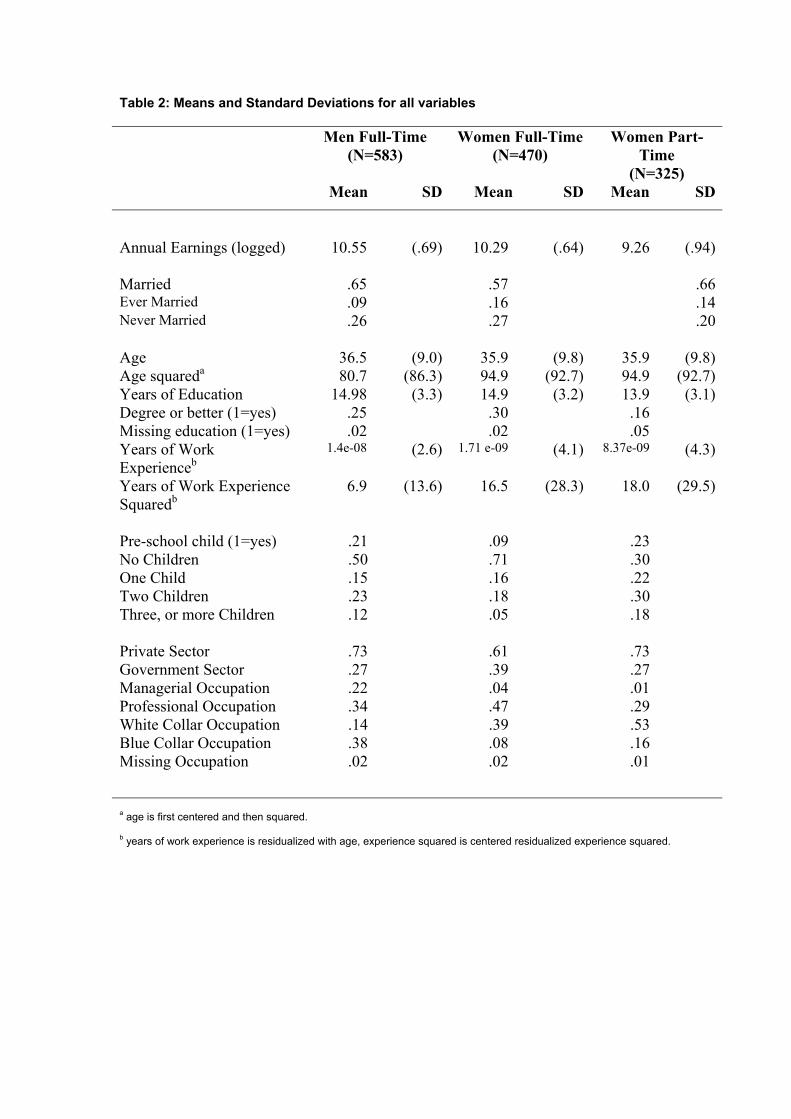
Table 2: Means and Standard Deviations for all variables
Men Full-Time (N=583)
Women Full-Time (N=470)
Women Part-Time
(N=325) Mean SD Mean SD Mean SD
Annual Earnings (logged) 10.55 (.69) 10.29 (.64) 9.26 (.94) Married .65 .57 .66 Ever Married .09 .16 .14 Never Married .26 .27 .20 Age 36.5 (9.0) 35.9 (9.8) 35.9 (9.8) Age squareda 80.7 (86.3) 94.9 (92.7) 94.9 (92.7) Years of Education 14.98 (3.3) 14.9 (3.2) 13.9 (3.1) Degree or better (1=yes) .25 .30 .16 Missing education (1=yes) .02 .02 .05 Years of Work Experienceb
1.4e-08 (2.6) 1.71 e-09 (4.1) 8.37e-09 (4.3)
Years of Work Experience Squaredb
6.9 (13.6) 16.5 (28.3) 18.0 (29.5)
Pre-school child (1=yes) .21 .09 .23 No Children .50 .71 .30 One Child .15 .16 .22 Two Children .23 .18 .30 Three, or more Children .12 .05 .18 Private Sector .73 .61 .73 Government Sector .27 .39 .27 Managerial Occupation .22 .04 .01 Professional Occupation .34 .47 .29 White Collar Occupation .14 .39 .53 Blue Collar Occupation .38 .08 .16 Missing Occupation .02 .02 .01
a age is first centered and then squared.
b years of work experience is residualized with age, experience squared is centered residualized experience squared.
Results
Table 3 presents results of the robust regression models. For ease of presentation we
only show coefficients for the marital status dummy variables. The baseline model
shows that full-time employed men have a significant marriage premium of
approximately 31 per cent of earnings, compared to never married men, and that men
who were previously married earn approximately 15 per cent more than never married
men. Adding human capital variables, as shown in Model 2, attenuates the return to
marriage for men by around half to 17 per cent. The association between previously
(ever) married men and wages becomes small and non-significant with the
introduction of human capital factors, and remains non-significant for all other
models. The R-squared also increases substantially (from 0.10 to 0.27) with the
introduction of human capital factors and increases marginally again with the
introduction of the job variables4. Adjusting for job characteristics (Model 3) and
family status (Model 4), in addition to human capital factors does not have a
significant effect on wages for married men. The final model includes human capital,
job characteristics and family status variables; after adjusting for all variables married
men earn around 14 per cent more than single men. We can thus account for about 55
per cent of the male full-time marriage premium with human capital, family and job
variables ((0.31-0.139) / 0.31 * 100).
In contrast to results for men, there is no significant association between
marriage and the wages of women employed full-time. This finding supports earlier
research using cross sectional data and ordinary least squares (OLS) regression
(Dolton & Makepeace 1987; Hill 1979; Korenman & Neumark 1992). There is a
small premium for previously (ever) married women that disappears once human
capital differences are controlled. For women employed part-time, however, the
baseline model (Model 1) shows a large significant association between marriage and
wages, with both currently and ever married women earning over thirty percent more
than never married women. Again, however, these differences can be fully accounted
for by human capital differences in married and single women. After controlling for
age, education and experience, there are no significant associations between marriage
and wages for part-time employed women in the remaining four models (Models 2-5).
Table 3: Marital status dummy coefficients for robust regression models
M1: Baseline Model
M2: Baseline & Human Capital
M3: Baseline, Human Capital &
Job Characteristics
M4: Baseline, Human Capital & Family Status
M5: All Variables
Full-time employed Men
Married .310** .174** .143** .189** .139** Ever Married .148* .053 .050 .054 .048 Never Married - - - - - Observations 583 583 583 583 583 R-squared .10 .27 .34 .27 .34 Full-time employed Women Married .080 .005 -.027 .018 -.011 Ever Married .120* .057 .034 .077 .059 Never Married - - - - - Observations 422 422 422 422 422 R-squared .01 .34 .40 .34 .41 Part-time employed Women Married .335** .100 -.017 .182 .084 Ever Married .381* .104 .089 .180 .178 Never Married - - - - - Observations 294 294 294 294 294 R-squared .03 .11 .16 .12 .18
*P<.05, **P<.01.
Consistent with earlier studies, our results thus show a significant positive
association between marriage and men’s average earnings. For women the
relationship between marriage and mean earnings tends to be small and non-
significant after adjusting for compositional differences in human capital. This is
again consistent with previous cross-sectional studies using OLS (Dolton &
Makepeace 1987; Hill 1979; Korenman & Neumark 1992). Studies examining the
determinants of women’s earnings more often find that motherhood, has a stronger
influence on women’s earnings than marriage, being associated with a substantial
wage penalty (Budig & England 2000; Waldfogel 1997). Models 4 and 5 included
dummy variables for the number of children, and presence of a pre-school child, but
our results (not shown) do not provide support for the wage penalty for motherhood
for either full-time or part-time women. As expected none of the family status
variables were significantly associated with men’s wages either.
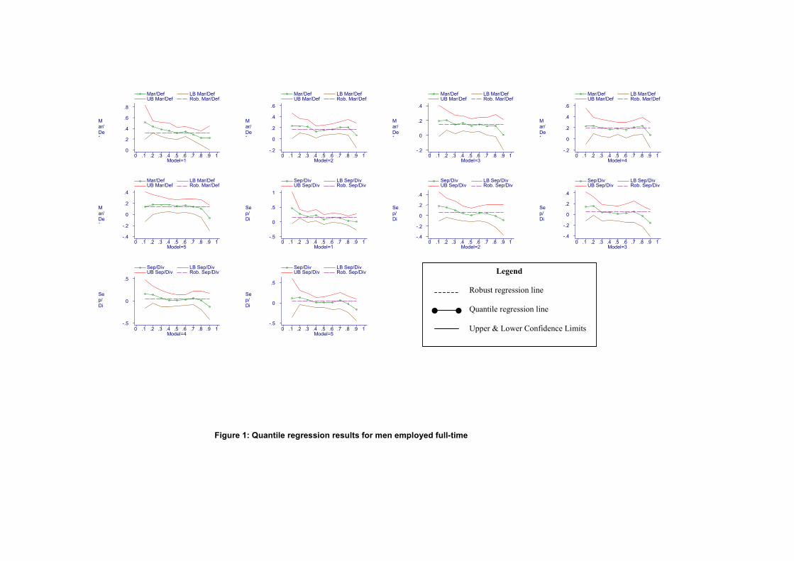
To further investigate the relationship between marriage and earnings and we
now turn to quantile regression models for the conditional deciles. Figures 1-3 present
graphs of the quantile regression coefficients for the five models separately for each
of the three subsamples. In each Figure, the first five graphs show the conditional
quantile regression coefficients for married respondents compared to never married
ones, while the next 5 graphs show the coefficients for those ‘ever previously
married’ (separated, divorced, widowed) compared to never married. For all graphs,
the dashed line represents the robust regression estimate (i.e. the relevant dummy
variable coefficient from the robust regression model), the dotted line is the
conditional quantile regression coefficient at each of the nine deciles, and the solid
lines are the upper and lower pointwise confidence limits for the quantile coefficients.
Where the confidence band incorporates zero the relationship between marriage and
earnings is not statistically significant. The figures also enable us to see how closely
the robust coefficient tracks the quantile coefficients along the earning distribution.
Figure 1 presents the results for men. For most models, the robust regression
coefficient tends to be within the quantile regression confidence band and to follow
the quantile estimates fairly closely. This suggests that the robust coefficients
generally estimate the marriage premium across the earnings distribution relatively
well. However, looking first at the marriage coefficients in figure 1 (first 5 panels) it
is also clear that the point estimates from the quantile regression tend to be larger than
the robust regression marriage premium in the lower deciles and smaller than it in the
higher deciles. In particular, men who are located at the top end of the wages
distribution tend to have smaller and non-significant returns to marriage, compared
with men in the middle of the wage distribution. This suggests that wage
determination processes vary somewhat across the male earnings distribution with
marriage mattering more at the bottom and middle and less at the top.
Figure 1: Quantile regression results for men employed full-time
Mar/Def
Model=1
Mar/Def LB Mar/Def UB Mar/Def Rob. Mar/Def
0 .1 .2 .3 .4 .5 .6 .7 .8 .9 1 0 .2 .4 .6 .8
Mar/Def
Model=2
Mar/Def LB Mar/Def UB Mar/Def Rob. Mar/Def
0 .1 .2 .3 .4 .5 .6 .7 .8 .9 1 -.2 0 .2 .4 .6
Mar/Def
Model=3
Mar/Def LB Mar/Def UB Mar/Def Rob. Mar/Def
0 .1 .2 .3 .4 .5 .6 .7 .8 .9 1 -.2
0
.2
.4
Mar/Def
Model=4
Mar/Def LB Mar/Def UB Mar/Def Rob. Mar/Def
0 .1 .2 .3 .4 .5 .6 .7 .8 .9 1 -.2 0 .2 .4 .6
Mar/Def
Model=5
Mar/Def LB Mar/Def UB Mar/Def Rob. Mar/Def
0 .1 .2 .3 .4 .5 .6 .7 .8 .9 1 -.4 -.2
0 .2 .4
Sep/Di
Model=1
Sep/Div LB Sep/Div UB Sep/Div Rob. Sep/Div
0 .1 .2 .3 .4 .5 .6 .7 .8 .9 1 -.5
0
.5
1
Sep/Di
Model=2
Sep/Div LB Sep/Div UB Sep/Div Rob. Sep/Div
0 .1 .2 .3 .4 .5 .6 .7 .8 .9 1 -.4 -.2
0 .2 .4
Sep/Di
Model=3
Sep/Div LB Sep/Div UB Sep/Div Rob. Sep/Div
0 .1 .2 .3 .4 .5 .6 .7 .8 .9 1 -.4 -.2
0 .2 .4
Sep/Di
Model=4
Sep/Div LB Sep/Div UB Sep/Div Rob. Sep/Div
0 .1 .2 .3 .4 .5 .6 .7 .8 .9 1 -.5
0
.5
Sep/Di
Model=5
Sep/Div LB Sep/Div UB Sep/Div Rob. Sep/Div
0 .1 .2 .3 .4 .5 .6 .7 .8 .9 1 -.5
0
.5 Legend
Robust regression line Quantile regression line Upper & Lower Confidence Limits
Figure 2 presents the corresponding graphs for full-time employed women.
They again show that the robust estimator models the relationship between marriage
and wages well at differing earnings levels. The patterning is similar to that for men,
where women at the top of the earnings distribution tend to have lower returns to
marriage than those in the middle, but overall the size of the coefficients are small.
The relationship between marriage and earnings tends to be non-significant across the
distribution and for all models, with one minor exception. Married women who are
situated in the 4th quantile have slightly higher returns to marriage than never married
women, which is significant for the first model. Women working full-time who were
previously married tend to have higher returns to earnings than never married women,
and the baseline model shows a significant relationship between being previously
married and earnings for women situated in the 6th, 7th and 8th quantiles.
Figure 2: Quantile regression results for women employed full-time
Mar/Def
Model=1
Mar/Def LB Mar/Def UB Mar/Def Rob. Mar/Def
0 .1 .2 .3 .4 .5 .6 .7 .8 .9 1 -.4 -.2
0 .2 .4
Mar/Def
Model=2
Mar/Def LB Mar/Def UB Mar/Def Rob. Mar/Def
0 .1 .2 .3 .4 .5 .6 .7 .8 .9 1 -.2
0
.2 Mar/Def
Model=3
Mar/Def LB Mar/Def UB Mar/Def Rob. Mar/Def
0 .1 .2 .3 .4 .5 .6 .7 .8 .9 1 -.4
-.2
0
.2
Mar/Def
Model=4
Mar/Def LB Mar/Def UB Mar/Def Rob. Mar/Def
0 .1 .2 .3 .4 .5 .6 .7 .8 .9 1 -.2
0
.2
Mar/Def
Model=5
Mar/Def LB Mar/Def UB Mar/Def Rob. Mar/Def
0 .1 .2 .3 .4 .5 .6 .7 .8 .9 1 -.4
-.2
0
.2
Sep/Di
Model=1
Sep/Div LB Sep/Div UB Sep/Div Rob. Sep/Div
0 .1 .2 .3 .4 .5 .6 .7 .8 .9 1 -.2 0 .2 .4 .6
Sep/Di
Model=2
Sep/Div LB Sep/Div UB Sep/Div Rob. Sep/Div
0 .1 .2 .3 .4 .5 .6 .7 .8 .9 1 -.2
0 .2
.4 Sep/Di
Model=3
Sep/Div LB Sep/Div UB Sep/Div Rob. Sep/Div
0 .1 .2 .3 .4 .5 .6 .7 .8 .9 1 -.2
0
.2
.4
Sep/Di
Model=4
Sep/Div LB Sep/Div UB Sep/Div Rob. Sep/Div
0 .1 .2 .3 .4 .5 .6 .7 .8 .9 1 -.2
0 .2 .4 .6
Sep/Di
Model=5
Sep/Div LB Sep/Div UB Sep/Div Rob. Sep/Div
0 .1 .2 .3 .4 .5 .6 .7 .8 .9 1 -.4 -.2
0 .2 .4
Legend
Robust regression line Qunatile regression line Upper & Lower confidence limits
Figure 3 presents results for women employed part-time. The robust
regression is also a good predictor of the relationship between marriage and earnings
for part-time employed women of different income levels. In Model 1, the
relationship between marriage and earnings is significant in the middle income
quantiles (3-7) for both married and previously married women. Further, part-time
women tend to have a larger earnings return to marriage than full-time women, but
generally the relationship is not significant. Overall, the quantile regressions tend to
support the findings of the robust regressions, showing virtually no association
between marriage and earnings for women irrespective of the amount they earn.
Figure 3: Quantile regression results for women employed part-time
Mar/Def
Model=1
Mar/Def LB Mar/Def UB Mar/Def Rob. Mar/Def
0 .1 .2 .3 .4 .5 .6 .7 .8 .9 1 -.5
0
.5
1
Mar/Def
Model=2
Mar/Def LB Mar/Def UB Mar/Def Rob. Mar/Def
0 .1 .2 .3 .4 .5 .6 .7 .8 .9 1 -.5
0
.5
1 Mar/Def
Model=3
Mar/Def LB Mar/Def UB Mar/Def Rob. Mar/Def
0 .1 .2 .3 .4 .5 .6 .7 .8 .9 1 -1 -.5
0 .5 1
Mar/Def
Model=4
Mar/Def LB Mar/Def UB Mar/Def Rob. Mar/Def
0 .1 .2 .3 .4 .5 .6 .7 .8 .9 1 -1
0
1
Mar/Def
Model=5
Mar/Def LB Mar/Def UB Mar/Def Rob. Mar/Def
0 .1 .2 .3 .4 .5 .6 .7 .8 .9 1 -1
0
1
2
Sep/Di
Model=1
Sep/Div LB Sep/Div UB Sep/Div Rob. Sep/Div
0 .1 .2 .3 .4 .5 .6 .7 .8 .9 1 -1
0
1 Sep/Di
Model=2
Sep/Div LB Sep/Div UB Sep/Div Rob. Sep/Div
0 .1 .2 .3 .4 .5 .6 .7 .8 .9 1 -1
0
1
2
Sep/Di
Model=3
Sep/Div LB Sep/Div UB Sep/Div Rob. Sep/Div
0 .1 .2 .3 .4 .5 .6 .7 .8 .9 1 -1
0
1
2
Sep/Di
Model=4
Sep/Div LB Sep/Div UB Sep/Div Rob. Sep/Div
0 .1 .2 .3 .4 .5 .6 .7 .8 .9 1 -1
0
1
2
Sep/Di
Model=5
Sep/Div LB Sep/Div UB Sep/Div Rob. Sep/Div
0 .1 .2 .3 .4 .5 .6 .7 .8 .9 1 -1
0
1
2 Legend
Robust regression line Quantile regression line Upper & lower confidence limits
Discussion
Our examination of the relationship between earnings and marriage shows a large and
significant marriage premium for men, but little or no association between marriage
and earnings for women. Adjusting for a range of human capital, job, and family
characteristics married men in our study earn 15 per cent more, on average, than
unmarried men. These findings support the findings of previous studies examining the
determinants of earnings for men, and other cross-sectional studies on the
determinants of women’s earnings (Blackburn & Korenman 1994; Dolton &