j ourna l homepage: www.e lsev ie r .com/ locate / rse
Marsh Dieback, loss, and recoverymappedwith satellite optical, airbornepolarimetric radar, and field data
Elijah Ramsey III a,⁎, Amina Rangoonwala b, Zhaohui Chi c, Cathleen E. Jones d, Terri Bannister c
a U.S. Geological Survey, National Wetlands Research Center, 700 Cajundome Blvd., Lafayette, LA 70506, USAb Five Rivers Services, LLC, 10807 New Allegiance Drive, Colorado Springs, CO 80918, USAc University of Louisiana-Lafayette CESU, 635 Cajundome Blvd, Lafayette, LA 70506, USAd Jet Propulsion Laboratory, California Institute of Technology, 4800 Oak Grove Dr., Pasadena, CA 91109, USA
Landsat ThematicMapper and Satellite Pour l'Observation de la Terre (SPOT) satellite based optical sensors, NASAUninhabited Aerial Vehicle synthetic aperture radar (UAVSAR) polarimetric SAR (PolSAR), and field data cap-tured the occurrence and the recovery of an undetected dieback that occurred between the summers of 2010,2011, and 2012 in the Spartina alterniflora marshes of coastal Louisiana. Field measurements recorded the dra-matic biomass decrease from 2010 to 2011 and a biomass recovery in 2012 dominated by a decrease of live bio-mass, and the loss of marsh as part of the dieback event. Based on an established relationship, the near-infrared/red vegetation index (VI) and site-specific measurements delineated a contiguous expanse of marsh diebackencompassing 6649.9 ha of 18,292.3 ha of S. alternifloramarsheswithin the study region. PolSAR datawere trans-formed to variables used in biophysical mapping, and of this variable suite, the cross-polarization HV (horizontalsend and vertical receive) backscatter was the best single indicator of marsh dieback and recovery. HV backscat-ter exhibited substantial and significant changes over the dieback and recovery period, tracked measuredbiomass changes, and significantly correlated with the live/dead biomass ratio. Within the context of regionaltrends, both HV and VI indicators started higher in pre-dieback marshes and exhibited substantially and statisti-cally higher variability from year to year than that exhibited in the non-diebackmarshes. That distinct differenceallowed the capturing of the S. alternifloramarsh dieback and recovery; however, these changeswere incorporat-ed in a regional trend exhibiting similar but more subtle biomass composition changes.
Saltmarshes are essential for terrestrial to ocean energy andnutrientexchanges, storm buffering, maintenance of water quality, and ashabitat and nursery for a myriad of wildlife and fish (Cullinan, LaBella,& Schott, 2004; Elmer et al., 2013; Zhang, Ustin, Reimankova, &Sanderson, 1997). Although they perform a critical dynamic role andhave intrinsic ecological importance, salt marshes face detrimentalpressures from natural and human-induced forces (Belluco et al.,2006; Cullinan et al., 2004; Elmer et al., 2013; Mendelssohn & McKee,1988; Zhang et al., 1997). Researchers have applied remote sensingmonitoring techniques to provide timely and synoptic status andtrend information that addresses the spatial heterogeneity and seasonalchanges of saltmarshes, (Belluco et al., 2006; Cullinan et al., 2004; Elmeret al., 2013; Mendelssohn &McKee, 1988; Wickland, 1991; Zhang et al.,
1997). Because biomass production is the primary indicator of saltmarsh health, remote sensing activities have focused on changes in bio-mass composition (e.g., Ramsey & Rangoonwala, 2005; 2006; 2010;Zhang et al., 1997). This paper describes remote sensing applied to thedetection and monitoring of Spartina alterniflora salt marsh biomasscomposition changes that revealed the occurrence and recovery of arecently observed phenomenon termed marsh dieback (Elmer et al.,2013; Ramsey & Rangoonwala, 2005; 2006; 2010).
Since the 1960s, S. alterniflora (smooth cordgrass) salt marshes thatdominate regularly flooded salt marshes of the Atlantic and Gulf coastsof the United States have been documented to experience scattered andirregularly timed periods of browning (chlorotic) leading in most casesto dead marsh and at times marsh loss (Bacon & Jacobs, 2013; Elmer,LaMondia, & Caruso, 2012; Kearney & Riter, 2011; McFarlin, 2012;McKee, Mendelssohn, & Materne, 2004; Mendelssohn & McKee, 1988;Ogburn & Alber, 2006). The driving factors shown to contribute to thedieback include water logging, drought, reduced flushing, herbivory,pathogens, and others (Bacon & Jacobs, 2013; Kearney & Riter, 2011;McFarlin, 2012;McKee et al., 2004;Mendelssohn&McKee, 1988); how-ever, the causes of dieback are likely varied and in most cases remainuncertain (Ogburn & Alber, 2006).
365E. Ramsey III et al. / Remote Sensing of Environment 152 (2014) 364–374
One of the largest (N100,000 ha) and intensely studied andreferenced marsh diebacks occurred in coastal Louisiana between2000 and 2001 and progressed for up to eight months after discovery(e.g., Bacon & Jacobs, 2013; McKee et al., 2004). Even though the2000–2001 Louisiana marsh dieback event was large and well-documented, satellite optical remote sensing detected and mapped amarsh dieback in 2008 that dwarfed that event (Ramsey, Werle,Suzuoki, Rangoonwala, & Lu, 2012). In the 2008 dieback, 111,000 ha offresh and 411,100 ha of salt marshes exhibited moderate to severemarsh dieback within three weeks of Hurricanes Gustav and Ike stormsurges impacting the Louisiana coastal region. Also in contrast to allother dieback occurrences, satellite radar remote sensing mappingshowed that the diebackwas the direct consequence of elevated salinityhurricane storm surges (Ramsey et al., 2012).
1.2. Optical and radar mapping of marsh dieback
The satellite remote sensing detection and mapping of the 2008dieback event were based on spectral methods developed as part ofthe 2000 Louisiana dieback study (Ramsey & Rangoonwala, 2005;2006; 2010). Chance observations leading to early detection of the2000 dieback provided the opportunity to apply remote sensing tech-niques to detect the occurrence of marsh dieback and to determinethe stage of dieback progression. Pigment concentrationswere analyzedat the plant-leaf scale along four transects covering the transition fromdead to healthy S. alterniflora to determine spectral changes indicativeof dieback onset and progression (Ramsey & Rangoonwala, 2005).Those plant-leaf transect results were then extrapolated to the plant-canopy scale in order to simulate aircraft and satellite spatial andspectral resolutions (Ramsey & Rangoonwala, 2006).
Our field studies confirmed the loss of the leaf chlorophyll pigmentwith marsh dieback noted by McKee et al. (2004) and related thepigment losses to leaf reflectance increases in visible reflectancemagni-tude, specifically in the blue (400–500 nm), green (500–600 nm) andred (600–700 nm) wavelength bands (Ramsey & Rangoonwala, 2005).The same study showed that although leaf water (spectral determina-tion after Peńuelas & Filella, 1998) and near-infrared (NIR, 700 to1300 nm) leaf reflectance magnitude decreased with dieback progres-sion, the relationships were weak and only clearly evident at a singlelate stage marsh dieback site (coefficient of determination, R2, of 0.35[leaf water] and 0.72 [NIR], p b 0.05) (Ramsey & Rangoonwala, 2005).In order to more fully account for site to site differences in diebackprogression, particularly the later stage exhibiting progressive NIRchanges, and provide a more reliable satellite remote sensing biophysi-cal measure, vegetation indexes (VI) calculated as the NIR/Green andNIR/Red ratios were applied (Ramsey & Rangoonwala, 2005; 2006). Inthis study we relied solely on the NIR/Red ratio as the marsh diebackindicator. Although the NIR/Green ratio performed slightly better inearlier stage diebacks, both NIR/Green and NIR/Red were good indica-tors of dieback progression, and NIR/Red performed better at laterstage diebacks at the plant-leaf scale (Ramsey & Rangoonwala, 2005).
The dieback progression explained 0.68 and 0.79 (R2, p b 0.10)and 0.82 and 0.85 (R2, p b 0.05) of the VI leaf-based reflectancevariance at the younger and later stage diebacks, respectively(Ramsey & Rangoonwala, 2005). A follow-on study extended theplant-leaf dieback results to the site-specific plant-canopy spectralchanges and found that aircraft and satellite remote sensing datacould distinguish (1) healthy marsh, (2) live marsh impacted bydieback, and (3) dead marsh, and provide some discrimination ofdieback progression (Ramsey & Rangoonwala, 2006). In addition,VI based on the NIR/Red band ratio reproduced hyperspectralplant-canopy indicators of marsh dieback at a 0.88 R2 (mean squareerror = 0.21) level (Ramsey & Rangoonwala, 2010). A final mappingof the 2000–2001 dieback event based on six Landsat ThematicMapper (TM) images collected before and after the dieback onsetaffirmed the necessity of atmospheric correction and conversion of
the remote sensing data to surface reflectance. Further, the TMdieback mapping emphasized that the most convincing evidence ofdieback impact or nonimpact is reflected in the temporal pattern ofthe vegetation index (Ramsey & Rangoonwala, 2010).
In remote sensing of vegetation, even if a pixel contains only a singleplant species (with similar leaf spectral properties), natural variabilityin the background (i.e., substrate, water) and canopy structure,(e.g., the plant orientation and density) along with leaf reflectance arecombined into the remote sensing reflectance (e.g., Huete & Jackson,1988; Jensen & Lorenzen, 1988; Peńuelas & Filella, 1998). The back-ground and structure contributions to the canopy reflectance, whichlikely have a varied relationship and importance to dieback occurrenceor progression, complicate linking of the leaf reflectance to canopyreflectance (Ramsey & Rangoonwala, 2006). Thus, in order to moredirectly link leaf optical indicators of dieback progression to canopy re-flectance, we need to determine indicators that account for or minimizecanopy structure and background influences in the canopy reflectancespectra.
While accounting for structure influences in the optical data ischallenging, synthetic aperture radar (SAR) mapping is largely directlyrelatable to the 3-dimensional distribution of water contained withinthe marsh leaves and stalks and underlying sediment (Dobson, Ulaby,& Pierce, 1995; Ramsey, 1998; Ramsey, 2005). SAR's sensitivity to the3-D water distribution as represented in the backscatter is illustratedin a mapping application closely related to the marsh dieback andrecovery. In that study, the near vertical stalk and leaf orientationsincreasingly exhibited in the early stages of marsh burn recoverybecame a denser and taller mix of horizontal and vertical orientations(relative to ground) as the recovery progressed (Ramsey et al., 1999).These changes in preferential orientation and increased density withincreasing time-since-burn were tracked with polarimetric SAR(PolSAR) L-band data collected from a P3 Orion aircraft operated bythe Naval Warfare Office (Ramsey et al., 1999). Initially, relativelyhigher VV (vertical send and receive) backscatter reflected thedominantly vertical regrowth. As growth progressed, VV backscatterdecreased relative to increased HH (horizontal send and receive)backscatter, and cross polarization, HV and VH, backscatterrepresenting the depolarized horizontal and vertical send radiation(Ramsey, Rangoonwala, Baarnes, & Spell, 2009a; Ramsey et al.,1999). Time-since-burn explained 73% (p b 0.01) of the VV/VHpower depolarization ratio representing nine marsh burn sites, andthe highest single polarization R2 of 0.83 (p b 0.01) was associatedwith VH backscatter (decibels) (Ramsey, Rangoonwala, Baarnes, &Spell, 2009a; Ramsey et al., 1999). VH was used as an indicator ofcanopy biomass variance.
Particularly relevant to this study, the single date PolSAR scenepredicted the time to complete marsh canopy recovery to be around1000 (±59) days (Ramsey, Rangoonwala, Baarnes, & Spell, 2009a;Ramsey et al., 1999). In contrast, a single date optical image estimatedonly 400 to 500 days until complete canopy recovery (Ramsey,Rangoonwala, Baarnes, & Spell, 2009a). It took temporal analyses ofnine TM images collected over five years to correctly predict marshcanopy recovery to be around 1000 (±88) days (Ramsey, Sapkota,Baarnes, & Nelson, 2002). A comparison of canopy reflectance andcanopy structural measurements collected over three years at one ofthesemarsh sites explains the advantage of SAR over opticalmonitoringin this case. While the canopy had recovered its stock of live biomass asrepresented by the optical reflectance spectra and lack of subsequentchange after one year of regrowth, the canopy structure differed sub-stantially from a fully mature canopy even after 1.5 years of regrowth(Ramsey, Rangoonwala, Baarnes, & Spell, 2009a). PolSAR's heightenedsensitivity to canopy structure as compared to optical imaging shouldprovide additional indicators of marsh dieback that enhance thedetection of dieback onset and monitoring of dieback progression,with the additional advantage of radar's all-weather and day-nightoperability.
366 E. Ramsey III et al. / Remote Sensing of Environment 152 (2014) 364–374
1.3. Data collections capturing the 2011 undetected dieback event
In support of yearly summer NASA Uninhabited Aerial Vehicle SAR(UAVSAR) flights over coastal Louisiana in response to the 2010Macondo-252 oil spill, non-impacted and impacted marsh sites locatedin the inland coastal zone were monitored nearly concurrently withUAVSAR flights in order to provide comparative baseline data. At twonon-oil-impacted S. alterniflora marshes, field measures collected aspart of this study showed an abrupt change in live to dead biomassfrom 2010 to 2011. At one site, a portion of the 2010 live marshremained while at the other site the healthy green marsh of 2010 wascompletely dead by the summer of 2011. The timing of the 2011diebackand juxtaposition of these sites with pre- and post-dieback PolSAR andfield data collections provided an excellent opportunity to test whetherPolSAR data could detect marsh dieback. Although only a limitedamount of satellite optical image data was available, this chance findingof marsh dieback also provided a challenging but ideal test of spectralmethods developed in the 2000–2001 coastal dieback to detect andmap the extent of this undetected dieback event. Together with thesetesting and validating opportunities is the near coincidental collectionpost-dieback of co-located PolSAR and field data, and, at one field site,concurrent, co-located optical image data.
1.4. Objectives
Near-coincident collections of field, satellite optical, and UAVSARPolSAR data during a 2010 to 2012 pre- to post-dieback period ofS. alterniflora marsh in coastal Louisiana formed the basis for thisstudy, for which the objectives were to (1) document site-specific
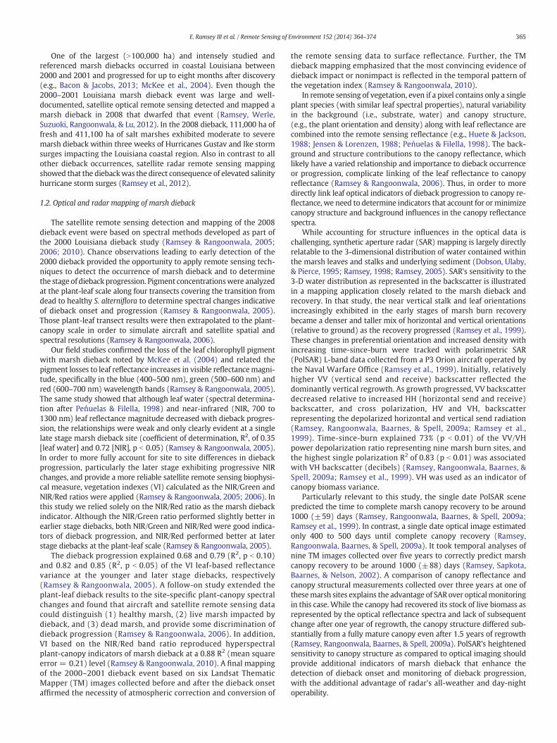
Fig. 1. Locationmapwith study area in Louisiana shown in the insets show a) the location of theGoogle Earth map.
changes in biomass associated with marsh dieback and recovery usingground based methods; (2) demonstrate the covariance betweenchanges in the optical VI based on the NIR/Red reflectance magnituderatio and marsh biomass composition; (3) extend the VI based site-specific relationship spatially and temporally with optical satellitedata; (4) determine the best single PolSAR based biophysical variableindicator of dieback and recovery based on site-specific biomassrelationships; and (5) relate regional changes of VI and the PolSARbased indicator within S. alterniflora dieback and non-dieback marshesover the 2010 to 2012 pre- to post-dieback period.
2. Study area
Located in the eastern deltaic plains of the north-central Gulf ofMexico, the study region encompasses estuarine wetlands (Sasser,Visser, Mouton, Linscombe, & Hartley, 2008) that include the44,447 ha area of interest (AOI) dominated by S. alterniflora marsh(Sasser, Visser, Mouton, Linscombe, & Hartley, 2014; Sasser et al.,2008) (Fig. 1). These marshes are scoured by hurricanes that can pushwater with elevated salinity into inland marshes, causing mortality(Neyland, 2007; Ramsey, Lu, Suzuoki, Rangoonwala, & Werle, 2011;Ramsey, Werle, Lu, Rangoonwala, & Suzuoki, 2009). Channels, levees,and impoundments constructed to provide transport conduits andwaterfowl sanctuaries impede overland flow and can lengthen marshexposure to elevated salinity surge water and, in the case of intenserainfall accompanying storm events, prolong inundation that promoteswater logging and subsequent marsh alteration and deterioration(Ramsey, Werle, Lu, Rangoonwala, & Suzuoki, 2009). The combination
study area with respect to the state and b) the location of the field sites inwhite dots on a
367E. Ramsey III et al. / Remote Sensing of Environment 152 (2014) 364–374
of low topographic relief, poorly drained soils, subsurface faulting, andflow hindrances creates a spatially complex hydrologic landscape.
3. Methods
3.1. Field measurements
Field data in 2010, 2011, and 2012 were collected within plots atsites 397 and 978 (see Fig. 1 inset b for site locations). Data collectionwithin the 30-m by 30-m plots followed a standard sampling strategythat provides reproducible measures within these structurally variablemarshes (for a detailed description see Ramsey, Nelson, Baarnes, &Spell, 2004). Vertical profiles (at a 20-cm increment from the bottomto the top of the canopy) of light attenuationwere obtained at a 3-m in-crement along the 30-m east–west and north–south transects. Biomasswas measured by clipping (a few centimeters above the surface) andgathering all standing marsh within a 1-m2 area chosen to representthe typical marsh at each site. Biomass samples were separated intolive and dead portions, dried, and weighed (for method details seeRamsey & Rangoonwala, 2005).
Due to the complete loss of marsh canopy by 2012 at site 978, fieldand image data collections were obtained at an alternate site 978Aclose to site 978 (located on Fig. 1). Although there was no expectationthat marsh at site 978A was exactly comparable to marsh at site 978 in2010 and 2011, regional visual reconnaissance suggested marsh at site978A provided a reasonable surrogate for marsh surrounding site 978experiencing regrowth in 2012.
At the times of the optical andPolSAR acquisitions,water levels at sites397 and 978 were obtained from hydrologic stations (within 356 mof sites 397 and 978) operated by the Coastwide Reference MonitoringSystemas described in the StrategicOnlineNatural Resources InformationSystem (SONRIS, 2009). Water levels were below the marsh ground sur-face at the times of all optical image collections but above the ground sur-face during the UAVSAR overflights. In order to adjust the biomass data toits above water value available for interactionwith the incident radar en-ergy, the site average leaf area index (LAI) profile was calculated. The cal-culation was based on an estimated site canopy vertical light extinctioncoefficient and the site average light attenuation profile (DecagonDevices, 2006). The site LAI profile was combined with the measuredabove ground water level to estimate the percent marsh canopy abovewater and the above water percent was used to adjust the biomassweights to above water biomass. Use of these adjusted biomass metricsofferedmore accurate depiction of PolSAR based variable and biomass re-lationships and improved interpretation of relationshipswhenportions ofthe marsh biomass were submerged.
3.2. Satellite optical image data
The results of the broadband canopy spectral analyses were imple-mented into the satellite detection and monitoring strategy (Ramsey& Rangoonwala, 2005; 2006). A search of optical satellite image data
Table 1NASA Uninhabited Aerial Vehicle SAR (UAVSAR), optical satellite images and field data collecti
Remote sensing
Sensor Date of collection Resolution (m)
UAVSAR 22 June 2010 5SPOT 30 July 2010 25UAVSAR 24 June 2011 5ETM+ 15 Aug 2011 25UAVSAR 1 July 2012 5ETM+b 29 May 2012 25
a Negative denotes below marsh surface.b Scattered clouds in the image.
that individually contained sites 397, 978 and 978A found eight LandsatEnhanced Thematic Mapper Plus (ETM+) (Global Visualization, 2012)and ten SPOT XS 4 and 5 (Earth Explorer, 2012) cloud-free or nearlycloud-free images available for the summer months from 2010 to2012. After excluding image dates and times where surface marshflooding and extensive cloud cover were present, two ETM+ imagesand one SPOT XS 4 image were identified to map the dieback event(Table 1). The Landsat ETM+ has a spatial resolution of 28.5 × 28.5-mand seven spectral bands; blue (0.45–0.52 μm), green (0.52–0.60 μm),red (0.63–0.69 μm), NIR (0.77–0.90 μm), two SWIR (1.55–1.75 μm and2.09–2.35 μm), and one thermal infrared (10.40–12.50 μm). SPOT XS 4has a spatial resolution of 20 × 20-m and four spectral bands; green(0.50–0.59 μm), red (0.61–0.68 μm), NIR (0.78–0.89 μm) and oneSWIR (1.58–1.75 μm). The ETM+ and SPOT NIR and Red bands wereused in the VI calculation.
3.2.1. Conversion to surface reflectanceData in the three selected images were converted to absolute units
(radiance) and a standard radiative transfer atmospheric correction(ATCOR) applied (Richter, 2010; Richter & Schläpfer, 2011). ATCOR re-quired the selection of the scattering phase function and an estimateof the horizontal visibility. The maritime scattering phase function waschosen to best reflect that summer atmospheric composition in sub-tropical latitudes. To provide an estimate of the horizontal visibility,we first calculated the total atmospheric optical depth as the sum ofoptical depth related to Mie or aerosol scattering obtained from Multi-sensor Aerosol Products Sampling System (MAPSS, 2013) and opticaldepth related to Rayleigh scattering estimated at standard atmosphericconditions (Elterman, 1970). The total optical depthwas transformed tohorizontal visibility estimates at 0.55 μ (Elterman, 1970; Ramsey &Nelson, 2005). With these inputs, the ATCOR radiative transfer modelapplied within the PCI image processing software package transformedthe at-sensor radiance measurements into marsh canopy reflectanceestimates providing fully comparable data across all three image dates(Richter, 2010; Richter & Schläpfer, 2011; PCI Geomatics, 2007).
Only one location provided a check of the performance of the atmo-spheric correction. The single location visually exhibited a relativelyhigh surface reflectance over the three image dates, and inspection onGoogle Earth indicated at least a portion of the surface remained non-vegetated. The pixels representing non-vegetated areas were extractedfrom the Red andNIR image bands for each of the three image dates andthe NIR/Red VI calculated for comparison (Table 2).
3.2.2. Image georectification and site-specific vegetation indexThe ETM+ and SPOT XS reflectance images were rectified to a
Universal Transform Mercator map projection. The image productsproduced by the rectification were resampled by using bilinear interpo-lation from the original 28.5 × 28.5-m (ETM+) and 20 × 20-m (SPOTXS) to a common 25 × 25-m pixel spatial resolution.
VI data from SPOTXS 2010 and ETM+2011 and 2012was extractedfor sites 397 and 978 using two pixels and four pixels respectively,
on dates covering Golden Meadows, Louisiana.
Ground-based observations
Above surface water depth (cm) Date of collection
Site 397 Site 978
15.5 11.3 397 8 June 2010−12.3a −10.4a 978 15 June 20106.4 21.0 397 2 June 2011−4.6a −4.4a 978 8 June 201132.3 31.7 397 21 June 2012N/A 0.0 978 21 June 2012
Table 2Surface reflectance and vegetation index (VI) data of a non-vegetated surface.
The location was chosen because it was non-vegetated and visually exhibited a fairly highsurface reflectance. Four pixels (25-m resolution)were used in the surface reflectance andVI average and standard deviation calculations for all three years using SPOT 4 for 2010and ETM + data for 2011 and 2012.
Table 4Biomass dryweightmeasurements andHVbackscatter extracted for the sites 397, 978 and978A (alternate site for 978 which converted to open water in 2012).
Site Year Live Dead Total Live/dead Remote sensing
368 E. Ramsey III et al. / Remote Sensing of Environment 152 (2014) 364–374
centered over the field collection areas. These VI data were compared toground biomass of each site as validation that the satellite image datacaptured the marsh dieback (Table 3).
3.3. PolSAR data collection and description
The PolSAR data for monitoring the marsh dieback and recoverywere made available through NASA's UAVSAR airborne strategic collec-tion in response to the Macondo-252 oil spill and in concern over itspossible long term detrimental effects on exposed coastal resources(Jones, Minchew, Holt, & Hensley, 2011; Ramsey, Rangoonwala,Suzuoki, & Jones, 2011). The day and night mapping capabilities offeredwith radar systems are further extended by the airborne platform offer-ing rapid response in emergencies and agility in tracking time-varyingfeatures. UAVSAR's precision repeat-track capability to within 5-m(Jones et al., 2011) enables direct comparison between revisit datacollections, and its high transmitted power results in a higher signal-to-noise ratio compared to satellite radars. The high signal-to-noiseratio, a quantity that indicates how much of the measured signalcomes from surface backscatter relative to what is generated by noisein the instrument electronics, is particularly important when using HVintensities, which are lower signal level than the HH or VV returns. Aprevious evaluation of the UAVSAR L-band data found that noise inten-sities remained below HV backscatter associated with marshes locatedin the near- to far-range with the possible exception of non-vegetatedland covers (Jones et al., 2011; Ramsey, Lu, Suzuoki, Rangoonwala, &Werle, 2011). The L-band 1217.5 to 1297.5 MHz (23.8 cm wavelength)frequency of the SAR system may provide more consistent subcanopyinformation as suggested in inundation flood mapping (Ramsey,Suzuoki, Rangoonwala, & Bannister, 2013; Ramsey et al., 2012), and itsfully polarized or quadrature polarized capability, recording intensitiesand phases of theHH, VV, and cross-polarization (HV and VH) backscat-ter, allow a more complete characterization of the scattering properties(McCandless & Jackson, 2004). Each of these unique UAVSAR capabili-ties can be critically important to monitoring subtle changes associatedwith marsh dieback in spatially complex land–water landscapes.
In this study, we used UAVSAR's ground range projected, calibrated,andmultilooked complex image data referred to as GRD (georeferenced)products (Zheng, Muellerschoen, Michel, Chapman, Hensley & Lou,2010). These image data reflect the amplitude and phase of the electro-magnetic wave measured by the PolSAR sensor representing the com-plex elements of the scattering matrix (Ramsey, Rangoonwala, Suzuoki,
Table 3Biomass dry weight measurements and optical data VI (NIR/Red) extracted for the sites397, 978 and 978A (alternate site for 978 which converted to mud flat in 2012).
Site specific: Biomass (g per m2) Remote sensing
Site Year Live Dead Total Live/dead Optical vegetation index (VI)
At site 978 (not shown) optical VI is 1.3 + 0.08 for the year 2012.
& Jones, 2011). The cross-polarized channels, HV and VH, are combinedinto a single channel based on the assumption that the HV and VH back-scatter is equal for natural surfaces (Van Zyl & Ulaby, 1990). Each GRDimage pixel represents ground resolutions of 5.338 m by 6.159 m inthe along track (azimuth) and cross track (range) directions, respective-ly, and an effective number of range and azimuth looks of 3 and 12, re-spectively. The GRD data were rectified to a UTMmap projection at a 5m by 5 m pixel resolution resulting in a higher spatial sampling of eachfield site than availablewith the optical image data. TheNASAGRDprod-uct provided a readily usable andhighfidelity polarimetric data source ofhigh spatial resolution and repeat targeting that enabled direct compar-ison and detection of subtle changes between the 2010, 2011, and 2012revisit data collections (Table 1), which was critical for the diebackmonitoring.
PolSAR data were extracted at each site by using a 5 by 5 (sites 397and 978A) and a 7 by 7 (site 978) pixel rectangle centered over the fieldcollection areas (Table 4). The 2010, 2011, and 2012 PolSAR data wereused to calculate mean HH, HV (combined HV and VH), and VV back-scatter intensities, HH/HV and VV/HV depolarization and HH/VV co-polarization ratios, and the HH–VV phase difference as a measure ofthe polarization properties of the marsh. In addition, we applied thestandard decomposition models (Cloude & Pottier, 1997; Freeman &Durden, 1997) to the complex polarimetric backscatter components ofthe GRD data in order to categorize the backscatter into distinct mecha-nisms (e.g., surface, volume, double bounce). Our application of PolSARdata was simplified to the identification of the best single variable,representing polarimetric intensity, intensity ratios, phase difference,or product of decomposition analysis, for determining changes in themarsh canopy associated with dieback and subsequent recovery.These measures should relate directly to the marsh structure and prop-erties, and thus, provide quantifiable measures of change (e.g., Ramsey,Rangoonwala, Suzuoki, & Jones, 2011).
3.4. Dieback extent and recovery
The extent of the dieback was determined by RGB color rendition ofpre- (2010) and post-dieback (2011) VI images; 2010 VI as red and2011 VI as the green and blue (Ramsey, Chappell, & Baldwin, 1997;Ramsey, Rangoonwala, Middleton, & Lu, 2009b). Abnormalities (highdifferences in reflectance) between the pre- (2010) and post-dieback(2011) VI images would exhibit the pre-dieback color defining the spa-tial extent of the abnormal VI decrease. Following previous studies, weexpected the 2010 color defining the dieback to include the two groundsites where diebackwas observed and extend beyond these two site lo-cations to identify the extent ofmarsh dieback. To transform the diebackcolor rendition into a quantifiable range of VImagnitudes,we calculatedthe 2010minus 2011 VI difference and defined all positive difference as
Site specific: Biomass(g per m2) corrected forwater depth at the timeof the UAVSAR collectiona
a Explanation is given in Section 3.1.b At site 978 (not shown), HV backscatter is 2.26E−04 indicating a total loss of canopy
by 2012. Recorded water level shows that site was under water at time of UAVSARcollection.
369E. Ramsey III et al. / Remote Sensing of Environment 152 (2014) 364–374
marsh dieback. The resultant dieback bitmap was converted to polygoncoverage for ease of comparability between the optical VI and PolSARHV images (PCI Geomatics, 2007). Similarly, S. alternifloramarsh withinthe study AOI but not in the dieback polygon was included in a non-dieback polygon. A minimummapping unit of 5 ha was used in the ras-ter to polygon conversions and upland areas andwater bodies were notincluded. The 2011minus 2012 VI differencewas used to portraymarshrecovery.
The 2010 to 2011 dieback marsh polygon was used to segment the2011 to 2012 VI map as well as the PolSAR images into dieback andnon-dieback areas for subsequent statistical analyses. These diebackand non-dieback analyses provided a perspective on the observedS. alternifloramarsh dieback within a regional and temporal context.
3.5. Documenting change and relationships
Paired two-tailed t-tests (SAS® Enterprise) were conducted to de-fine changes of site-specificfield and image-based biophysicalmeasuresused to describe changes related to the dieback and recovery. Each t-testfirst considered the equality of the population variance and then usedthe appropriate t-test based on the variance equality test and the de-grees of freedom (df) and p value reported. Scatter plots were used toshow the simple relationships between field biophysical measures andsite-specific optical and PolSAR site means in order to extend the fieldbiophysical changes supporting marsh dieback and recovery to theimage coverages. Optical site-specific imagemeans were plotted versusthe field biophysical measures, while PolSAR site-specific means wereplotted versus thefield biophysicalmeasures corrected forwater depthsat the time of the PolSAR collection. Statistical analyses based on themeans calculated for the two segments were conducted to test whether
Fig. 2. Site photos obtained in 2010, 2011, and 2012 showing Spartina alternifloramarsh at siteversion of site 978 to mud flat, site 978A (g) representing the same marsh and with generally
differences in the mean responses existed within and between diebackand non-dieback marshes and years for optical VI and PolSAR diebackindicators.
4. Results
4.1. Consistency of the surface reflectance estimates
VIs calculated from Red and NIR reflectance extracted from a singlenon-vegetated surface location were 0.96, 1.05, and 1.05 in 2010,2011, and 2012, respectively (Table 2). Even though the exact condi-tions of the non-vegetated surface are unknown, these results indicatethat the atmospheric correction and subsequent NIR/Red band ratio cal-culation provided a consistent VI representation of the surface conditionover the three optical image dates.
4.2. Field data analysis results and relationships to image data
4.2.1. Changes in total, live, and dead biomassSite photographs showed dramatic changes in canopy condition at
sites 397 and 978 from 2010 to 2011 accompanying the marsh dieback(Fig. 2). Biomassmeasures at both ground sites captured these dramaticchanges (Table 3). Total biomass nearly equal in 2010 at sites 397 and978 had decreased by a factor of three at both sites by 2011. Livebiomass had dramatically decreased by 2011 becoming nearly absentat site 978 and reduced to less than one-fourth its 2010 level at site397. At both sites in 2011, dead biomass was approximately half of its2010 level (Table 3).
Field measures showed a general recovery of the S. alternifloramarshes by 2012; however, marsh at site 978, which was nearly 100%
s 397 (a, c, e) and 978 (b, d, f). Green is live and brown is dead marsh. Because of the con-the same site conditions was substituted.
370 E. Ramsey III et al. / Remote Sensing of Environment 152 (2014) 364–374
dead in 2011, was converted to a mud flat with stubble (ca. b10 cm)that was submerged at high tide (Table 3, Fig. 2). In 2012, total biomassat site 397 and at site 978A, representing regrownmarsh in the vicinityof site 978, had recovered to two-thirds of their 2010 weights domi-nantly by an addition of live biomass. The substantially higher increasein live biomass relative to the much smaller addition of dead biomassresulted in the live to dead ratio increasing to above 2010 levels by2012, particularly at site 397 (Table 3).
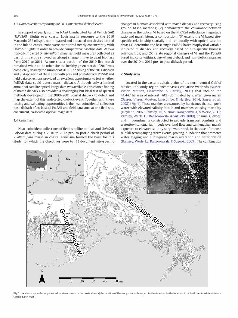
Fig. 4.The negative relationship betweenHVbackscatter and the canopy abovewater live/dead biomass composition at each field site over the three collection years provided thehighest explanatory relationship R2 = 0.84, n = 6, p b 0.01.
4.2.2. Site-specific optical data relationships to field dataVI variance over the three years exhibited high correlations to
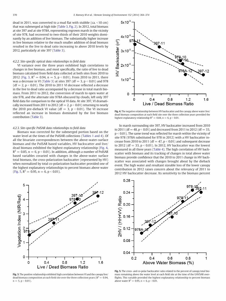
changes in live biomass, and most specifically, the ratio of live to deadbiomass calculated from field data collected at both sites from 2010 to2012 (Fig. 3, R2 = 0.94, n = 5, p b 0.01). From 2010 to 2011, therewas a decrease in VI (Table 3) at sites 397 (df = 3, p b 0.01) and 978(df = 2, p b 0.01). The 2010 to 2011 VI decrease reflected a decreasein the live to dead ratio accompanied by a decrease in total marsh bio-mass. From 2011 to 2012, the conversion of marsh to open water atsite 978, and the alternate site 978A obscured by clouds, left only 397field data for comparison to the optical VI data. At site 397, VI dramati-cally increased from 2011 to 2012 (df= 2, p b 0.01) returning to nearlythe 2010 pre-dieback VI value (df = 3, p b 0.01). The VI increasereflected an increase in biomass dominated by the live biomasscontribution (Table 3).
4.2.3. Site-specific PolSAR data relationships to field dataBiomass was corrected for the submerged portion based on the
water level at the times of the PolSAR collections (Tables 1 and 4). Ofall the bivariate correspondences between the above-water-surfacebiomass and the PolSAR based variables, HV backscatter and live/dead biomass exhibited the highest explanatory relationship (Fig. 4,R2 = 0.85, n = 6, p b 0.01). In addition, although a number of PolSARbased variables covaried with changes in the above-water surfacetotal biomass, the cross-polarization backscatter (represented by HV)when normalized by total co-polarization backscatter provided one ofthe highest explanatory relationships to percent biomass above water(Fig. 5, R2 = 0.95, n = 6, p b 0.01).
Fig. 3.The positive relationship exhibited high correlation betweenVI and the canopy live/deadbiomass composition at each field site over the three collection years (R2= 0.94,n = 5, p b 0.01).
In marsh surrounding site 397, HV backscatter increased from 2010to 2011 (df=48, p b 0.01) and decreased from 2011 to 2012 (df= 33,p b 0.01). The same trend was reflected for marsh within the vicinity ofsite 978 (978A substituted for 978 in 2012) with a HV backscatter in-crease from 2010 to 2011 (df = 47, p b 0.01) and subsequent decreaseto 2012 (df = 33, p b 0.01). In 2012, HV backscatter was the lowestmeasured in all three years (Table 4). The high correlation of HV back-scatter with biomass and its tracking of changes in total above waterbiomass provide confidence that the 2010 to 2011 change in HV back-scatter was associated with changes brought about by the diebackevent. The high water and resultant sizeable loss of the lower canopycontribution in 2012 raises concern about the relevancy of 2011 to2012 HV backscatter decrease. Its sensitivity to the biomass percent
Fig. 5. The cross- and co-polar backscatter ratio related to the percent of canopy total bio-mass remaining above the water level at each field site at the time of the UAVSAR over-flights. This variable provided the highest explanatory relationship to percent biomassabove water R2 = 0.95, n = 6, p b 0.01.
Fig. 7. a) RGB color rendition of pre- (2010) and post-dieback (2011) VI images, 2010 VIwas rendered as red and 2011 VI as the green and blue. The red tone illustrates the extentof marsh dieback and bluish tones the non-diebackmarshes. b) The 2012 VIwas rendered
371E. Ramsey III et al. / Remote Sensing of Environment 152 (2014) 364–374
remaining above water, however, indicates that at least part of the HVbackscatter was not a function of the changing portions of submergedbiomass and was instead associated with the marsh recovery.
4.2.4. Site-specific VI and HV relationshipThe final appraisal of HV backscatter as an indicator of marsh
dieback, and particularly, as an indicator of marsh dieback recoverywas conducted by comparison of the correlation of HV backscatter andVI changes reflecting the 2010 to 2011 dieback and 2011 to 2012recovery (Fig. 6, R2 = 0.89, n = 5, p b 0.01).
4.3. VI changes in dieback and non-dieback marshes
The AOI area was segmented into S. alterniflora dieback (6649.9 ha)and the non-dieback (11,642.4 ha) marsh polygons discussed inSection 3.4. The 2010 to 2011 VI decrease in S. alterniflora and a subse-quent recovery of those marshes from 2011 to 2012 were also shownby running t-tests (Fig. 7a and b). The mean VI of pixels containedwithin the dieback polygon decreased from 2.67 in 2010 to 1.73 in2011 (df = 1.23 × 10⁵, p b 0.01) and subsequently increased to 2.87 by2012 (df= 1.09 × 10⁵, p b 0.01). Non-diebackmarsh VI meansincreasedslightly from 2.19 in 2010 to 2.24 in 2011 (df= 4.34 × 10⁵, p b 0.01) andexhibited amore substantial increase to 2.78 in 2012 (df= 3.15 × 10⁵,p b 0.01). Differences calculated from 2010 to 2011 and 2012 to 2011were 0.971 and 1.01 for dieback VIs (df = 1.89 × 10⁵, p b 0.01), respec-tively, and 0.001 and 0.514 for non-dieback VIs (df = 3.82 × 10⁵,p b 0.01), respectively.
4.4. HV changes in dieback and non-dieback marshes
Marsh dieback was calculated as the 2010–2011 difference (Fig. 8a),and marsh recovery as the 2011–2012 difference in the HV backscatter(Fig. 8b) (Table 4). The mean HV backscatter of pixels containedwithin the dieback polygon increased from 3.06 × 10⁻³ in 2010 to4.21 × 10−3 in 2011 (df = 3.73 × 10⁶, p b 0.01) and subsequentlydecreased to 1.91 × 10−3 by 2012 (df = 3.73 × 10⁶, p b 0.01). Non-dieback marsh pixels increased moderately from 2.34 × 10⁻³ in 2010to 2.88 × 10⁻³ in 2011 (df = 6.59 × 10⁶, p b 0.01) and exhibiteda substantial decrease to 2.11 × 10⁻³ in 2012 (df = 6.23 × 10⁶,p b 0.01). Differences calculated from 2010 to 2011 and 2012
Fig. 6. The negative correspondence between HV backscatter and VI at the two field sitesover the three study years. This depiction proved HV as an indicator of marsh dieback re-covery which could be used as a VI equivalent proxy (R2 = 0.89, n = 5, p b 0.01).
as red and 2011 VI as the green and blue. The red tone illustrates the extent of marsh re-covery. Even though of lower contrast, the pattern of red hues represents the 2011 to 2012VI increase indicating a marsh recovery. Water (in black), upland and clouds (in 2012ETM+ image) (in white) were excluded from all VI analyses. The inset locates the fieldsites. The white box outlines the AOI.
to 2011 were−1.18 × 10⁻³ and−2.37 × 10⁻³ for dieback HVs(df = 3.67 × 10⁶, p b 0.01), respectively, and−0.55 × 10⁻³
and−0.811 × 10⁻³ for non-dieback HVs (df = 6.47 × 10⁶, p b 0.01),respectively.
5. Discussion
Field and satellite optical data conclusively revealed and mapped adieback that occurred between the summers of 2010 and 2011 andthe following 2012 recovery in the S. alterniflora marshes of coastalLouisiana. Although previous studies established marsh dieback bio-physical indicators amenable to remote sensing, a shortcoming in map-ping the2000–2001 and 2008 dieback eventswas the lack of concurrentfield and image data collections before and after each event (Ramsey &Rangoonwala, 2005; 2006; Ramsey et al., 2012). In this study, biomasschanges were directly measured before and one year after the diebackevent. These field measures captured the dramatic decrease in biomassand live to dead biomass composition accompanying the 2010 to 2011dieback, the reversal of biomass composition signifying a recovery pro-gression by 2012 (Table 3), and a dramatic conversion of healthymarsh
Fig. 8. UAVSAR HV backscatter a) 2010 and 2011 difference image and b) 2012 and 2011difference image overlain with the VI dieback polygon vector (in white). The lighter graytone depicts the extent of marsh dieback (and subsequent recovery) and dark gray non-dieback marshes. Water (in black) and upland (in white) were excluded from all HVanalyses. The insets show field site locations. The white box outlines the AOI.
372 E. Ramsey III et al. / Remote Sensing of Environment 152 (2014) 364–374
in 2010 to mud flat by 2012 (Fig. 2, Table 3). The documentation of bio-physical changes accompanying the dieback and recovery progressionand dramatic marsh loss provides unique insight into the mechanismofmarsh dieback and loss, and establishes what biophysical changes re-mote sensing methods could reliably monitor to detect and map thedieback progression.
Results of this study reinforced the utility of optical VI based on theNIR/Red ratio to map marsh diebacks (Ramsey, Lu, Suzuoki,Rangoonwala, & Werle, 2011; Ramsey & Rangoonwala, 2005; Ramsey& Rangoonwala, 2006). Those previous studies applied transect strate-gies and direct mapping of elevated salinity surge waters to link VIchanges to dieback onset and progression. In this study, near-concurrent collection of biophysical and satellite data in concert withthe marsh transition from healthy to dieback to recovery provided thecapability for direct covariance analyses. As indicated in the previousVI dieback mapping and substantiated in numerous remote sensingstudies that mapped biomass with a variety of near-infrared and visibleband ratios (He, Guo, & Wilmshurst, 2007; Huete, Justice, & Leeuwen,1999; Vogelmann, Rock, & Moss, 1993), we found that the live biomasscomponent dominantly influences the VI variance (Fig. 3, Table 3).These results provide conclusive evidence that the remote sensing VIis a direct indicator of marsh biophysical changes defining dieback andrecovery.
Site-specific biophysical and VI relationships extended regionally byusing three consecutive years of satellite optical image data showed thatbiomass composition as represented byoptical-basedVImagnitude var-ied spatially but the yearly pattern of change was not spatially consis-tent throughout the S. alterniflora marshes. The two field sites wereencompassedwithin a nearly contiguous 6649.9 ha ofmarsh that exhib-ited the dieback and recovery pattern of VI decrease and subsequent in-crease. Outside this dieback marsh region, however, 11,642.4 ha ofsurrounding non-dieback marsh did not exhibit the dieback VI pattern;this was also supported by the statistical results.
Regional analyses found that from 2010 to 2011 dieback marsheshad a substantial average VI decrease compared to practically no changein non-dieback marshes. By 2012, VI increased in dieback marshes tonearly pre-dieback VI magnitudes and non-dieback marshes had a VIincrease about half that. Basically, the 2010 to 2011 dieback and non-dieback marsh difference in VI decrease was the single factor thatidentified the dieback. That decrease difference, however, began fromdifferent starting points. On average, VI was nearly 0.5 units higherin pre-dieback marsh than in non-dieback marsh in 2010. The nearly2-fold higher VI increase in 2012 in dieback marshes compared tonon-dieback marshes brought the VI levels, and by extension, the livebiomass composition levels into near alignment. To determinewhetherthe initial VI difference was a precursor to the dieback onset, however,was not part of this study. What was determined was that VI mappingcaptured a dieback event including eventual marsh loss that differen-tially occurred in S. alterniflora marshes exhibiting higher pre-diebackVIs than non-dieback marshes.
Assessment of the PolSAR based single variable and biomass mea-sures adjusted for above-surface-water levels found that HVbackscatterprovided the best single variable indicator of biomass changes accom-panying marsh dieback and recovery. HV backscatter as an indicator ofdepolarization of the co-polarized data (HH and VV) originates mainlyfrommultiple scattering within the canopy and has reported sensitivityto forest and agriculture biomass (Brakke, Kanemasu, & Steiner, 1981;Ferrazzoli et al., 1997; Ghasemi, Sahebi, & Mohammadzadeh, 2011;Westman & Paris, 1987). L-band backscatter is sensitive to grasslandbiomass (Dobson, Pierce, & Ulaby, 1996), and studies have demonstrat-ed direct correspondence between L-band polarimetric radar HV back-scatter and grassland biomass measures. Dabrowska-Zielinska et al.(2014) found strong per-class linear relationships between the canopyLeaf Area Index, a proxy of biomass, and HV backscatter. Herold,Schmullius, and Hajnsek (2001) found that of the three polarizationsHV backscatter provides the highest sensitivity to grassland canopyfeatures and the highest explanation of plant water content (an indica-tor of live biomass). Results of those studies concur with resultsreported here that indicate the potential of HV backscatter to providegrassland biomass information. However, the nature of its relationshipto changes in herbaceous (grasses) land cover remains less clear thanfor the more fully studied forest and agriculture landcovers.
Another factor is the influence of decreased above-water biomass.As seen in Table 4, HV backscatter from surface water covering marshstubble (site 978 in 2012)was over six times lower thanHV backscatterfrom site 978Awith only 28% of its total biomassweight of nearly 1.1 kgexposed. Even with a majority of the marsh canopy submerged,above water biomass produced an appreciable increase in thecross-polarized HV backscatter. Further, HV backscatter magnitudewas similar at site 397 in 2012, and in 2011, both sites 397 and 978exhibited dramatically higher HV backscatter with comparabletotal biomass quantities. It is likely that some portion of the 2011to 2012 decrease in HV backscatter was related to the change inlive biomass composition representing marsh recovery.
HV backscatter extracted from sites 397 and 978 (978A) changedsignificantly from year to year (Table 4). Somewhat counterintuitivelybecause of its expected positive relationship with canopy density, HVbackscatter increased with the decrease in marsh biomass 2010 to2011 and decreased with regrowth from 2011 to 2012. Following
373E. Ramsey III et al. / Remote Sensing of Environment 152 (2014) 364–374
this negative relationship with canopy dieback and regrowth, HV back-scatter exhibited a significant negative correlation with live biomasscomposition (Fig. 6). Ongoing analyses are pursuing specific detailsconcerning the nature of HV backscatter correspondence with biophys-ical changes accompanying themarsh dieback. However, even if not yetfully explained, site-specific evidence of substantial changes in accor-dance with the dieback and recovery pattern and its correspondencewith changes in live biomass is strong even though inferential.
Average HV backscatter within the dieback marshes showed a sub-stantial increase from 2010 to 2011 and a dramatic reversal from 2010to 2011. HV backscatter also increased in non-dieback marshes from2010 to 2011 but by less than half the amount of dieback marshes.The HV backscatter decrease in non-dieback marshes was moresubstantial from 2011 to 2012 but still only a third of the change in die-backmarshes. HV backscatter started out higher in the diebackmarshesin 2010 but the dieback and non-dieback marshes ended in 2012 withsimilar average HV backscatter magnitudes. The overall pattern ofchange, although negatively correlated, tracked theVI pattern. Althougha small change from 2010 to 2011 and even a more substantial from2011 to 2012 occurred, the change in non-dieback marshes is stillsmall in comparison to those in dieback marshes.
Both VI and HV backscatter show different starting points in the twomarshes in 2010 and more dramatic changes of their values from 2010to 2011 and again from 2011 to 2012 in dieback as compared to non-dieback marshes. Individually, VI and HV ended nearly equal in thetwo marshes by 2012. Changes in VI are substantiated to track changesin marsh live biomass composition as a direct indicator of dieback.While not all changes in live biomass composition define a diebackevent, the dramatic biomass changes shown to be in accordance withVI site-specific changes proved that VI mapping based on satelliteSPOT XS and Landsat ETM+ image data captured an undetected andextensive region of S. alterniflora dieback. HV backscatter tracked livebiomass composition and VI site-specific changes and closely emulatedVI dieback and non-dieback marsh regional patterns. The highervariability of VI and HV backscatter within the defined dieback marshesas compared to the non-dieback marshes may provide the pattern thatidentifies these events.
6. Conclusion
VI changes based on satellite SPOT and ETM+ image data trans-formed to surface reflectance and validated by site-specific measure-ments detected and mapped a sizeable (6649.4 ha) and undetectedS. alterniflora marsh dieback event in coastal Louisiana between 2010and 2012. The VI changes were shown to directly co-vary with field-measured changes in the live biomass composition, and the live biomasscomposition to represent changes in the marsh canopy related to die-back and its recovery.While not all changes in live biomass compositiondefine a dieback event, dramatic biomass changes accepted asindicators of dieback were confirmed to be in accordance with VI site-specific changes. These results reinforce the established utility of opticalVI to mapmarsh diebacks. The detection and mapping of a sizeable andundetected sudden marsh dieback event establish the capability ofmoderate spatial resolution satellite optical data to provide criticalcoastal resource status and trend information that is not always obtain-able by field observations or intermittent aerial photographic surveys.
The juxtaposition of the NASA UAVSAR PolSAR data collections forthe three summers that encompassed the dieback was used to demon-strate the correlation among the field, optical, and PolSAR data sourcesand their relationship to the marsh dieback and recovery. We foundthat the single best PolSAR based indicator of marsh dieback and recov-ery was the cross-polarized (HV) backscatter. HV backscatter exhibitedsubstantial and significant changes over the dieback and recovery peri-od tracking changes in biomass, represented as changes in the live bio-mass composition. As in VI, HV backscatter significantly correlated,although negatively, to changes in live and dead biomass ratio.
VI and HV backscatter exhibited similar initial and change patternswithin and between S. alterniflora dieback and non-dieback marshes.Initial starting points for each were higher in the dieback marshes andVI as well as HV backscatter means calculated for the 2012 diebackand non-dieback marshes were similar. Overall, the dieback marsheswere associated with and detected by substantially higher changes ascompared to themuchmore subtle but largely similar pattern of chang-es occurring in non-dieback marshes. The possibility that dramatic bio-physical changes accompanying dieback events can be encased withinspatially extensive regional trends similar in pattern but much moresubtle is a critical result of this study. Along with the capture of anextensive and undetected dieback with satellite optical data, anothercritical result of this study is that radar based image data may providedirect mapping of marsh dieback.
Work is ongoing particularly in specifying the HV backscatter rela-tionship to canopy composition and influences of flooding; however, re-sults of this study demonstrate a high potential for nearly all-weatherand day and night operable SAR systems like the targeted, high fidelity,high signal to noise and high spatial resolution UAVSAR PolSAR systemto identify canopy structure changes that may portend damaging die-back events. Targeted PolSAR and optical imaging could advance boththe canopy biophysical detail and mapping consistency necessary forcapturing heightened changes within a pattern of regional changes.
Acknowledgement
We thank Francis Fields Jr. of the Apache Louisiana Minerals LLC, asubsidiary of Apache Corporation, for access to their properties. Wealso thank Ryan Longhenry, Data Management Specialist, U.S. Geologi-cal Survey (USGS), Earth Resources Observation and Science (EROS)Center and CarolynGacke, contractor Science Applications InternationalCorporation at USGS EROS Center for the help and support in providingthe SPOT satellite data. We appreciate the help by Sijan Sapkota of theU.S. Geological Survey for his assistance in developing statisticalmodels.We appreciate the review of the manuscript by John Iiames, ResearchBiologist at U.S. Environmental Protection Agency, and Dirk Werle ofAERDE Environmental Research, Canada. We also thank the two anony-mous reviewers for their exhaustive, judicious and perceptive reviews.Research was supported in part by National Aeronautics SpaceAdministration (NASA) grant #11-TE11-104 and was carried out incollaboration with the Jet Propulsion Laboratory, California Institute ofTechnology, under a contract with NASA. Any use of trade, firm, orproduct names is for descriptive purposes only and does not implyendorsement by the U.S. Government.
References
Bacon, C., & Jacobs, A. (2013). Sudden wetland dieback in Delaware's inland bays. (URL).http://deestuaryarchive.mobiusnm.com/scienceandresearch/Science_Conf/Conference_Presentations/DESC07_No16_Bason.pdf (accessed: 18 March 2013).
Belluco, E., Camuffo, M., Ferrari, S., Modenese, L., Silvestri, S., Marani, A., et al. (2006).Mapping salt-marsh vegetation by multispectral and hyperspectral remote sensinga. Remote Sensing of Environment, 105, 54–67.
Brakke, T., Kanemasu, E., & Steiner, J. (1981). Microwave radar response to canopy mois-ture, leaf-area index, and dry weight of wheat, corn and sorghum. Remote Sensing ofEnvironment, 11, 207–220.
Cloude, S., & Pottier, E. (1997). An entropy based classification scheme for land applica-tions of polarimetric SAR. IEEE Transactions on Geoscience and Remote Sensing, 35,68–78.
Cullinan, M., LaBella, N., & Schott, M. (2004). Salt marshes — A valuable ecosystem. TheTraprock, 3, 20–23.
Dabrowska-Zielinska, K., Budzynska, M., Tomaszewska, M., Bartold, M., Gatkowska, M.,Malek, I., et al. (2014). Monitoring wetlands ecosystems using ALOS PALSAR(L-Band, HV) supplemented by optical data: A case study of Biebrza wetlandsin northeast Poland. Remote Sensing, 6(2), 1605–1633.
Devices, Decagon (2006). Operators manual; AccuPAR model LP-80 PAR/LAI ceptometer.Pullman, WA: Decagon Devices, Inc.
Dobson, C., Pierce, L., & Ulaby, F. (1996). Knowledge-based land-cover classification usingERS-1/JERS-1 SAR composites. IEEE Transactions on Geoscience Remote Sensing, 34(1),83–99.
374 E. Ramsey III et al. / Remote Sensing of Environment 152 (2014) 364–374
Dobson, C., Ulaby, F., & Pierce, L. (1995). Land-cover classification and estimation ofterrain attributes using synthetic aperture radar. Remote Sensing of Environment, 51,199–214.
Elmer, W., LaMondia, J., & Caruso, F. (2012). Association between Fusarium spp. onSpartina alterniflora and dieback sites in Connecticut and Massachusetts. Estuariesand Coasts, 35, 436–444.
Elmer, W., Useman, S., Schneider, R., Marra, R., LaMondia, J., Mendelssohn, I., et al. (2013).Sudden vegetation dieback in Atlantic and gulf coast salt marshes. Plant Disease,97(4), 436–445.
Elterman, L. (1970). Vertical-attenuationmodel with eight surface meteorological ranges 2 to13 kilometers. Air Force Cambridge Research Laboratories (AFCRL-70-0200, 56p).
Earth Explorer (2012). U.S. Geological Survey. (URL) http://earthexplorer.usgs.gov(accessed 11 November 2012).
Ferrazzoli, P., Paloscia, S., Pampaloni, P., Schiavon, G., Sigismondi, S., & Solimini, D. (1997).The potential of multifrequency polarimetric SAR in assessing agricultural and arbo-reous biomass. IEEE Transactions on Geoscience and Remote Sensing, 35(1), 5–17.
Freeman, A., & Durden, S. (1997). A three component scattering model for polarimetricSAR data. IEEE Transactions on Geoscience and Remote Sensing, 36, 963–973.
Ghasemi, N., Sahebi, M., & Mohammadzadeh, A. (2011). A review on biomass estimationmethods using synthetic aperture radar data. International Journal of Geomatics andGeosciences, 1(4), 776–788.
Global Visualization (2012). U.S. Geological Survey. (URL) http://glovis.usgs.gov(accessed: 10 October 2012).
He, Y., Guo, X., &Wilmshurst, J. F. (2007). Comparison of different methods for measuringleaf area index in a mixed grassland. Canada Journal of Plant Science, 87, 803–813.
Herold, M., Schmullius, C., & Hajnsek, I. (2001). Multifrequency and polarimetric radarremote sensing of grassland — Biophysical and landcover parameter retrieval withE-SAR data. In M. F. Buchoithner (Ed.), A decade of trans-European remote sensingcooperation (pp. 95–101). CRC Press.
Huete, A.R., & Jackson, R. (1988). Soil and atmosphere influence on the spectra of partialcanopies. Remote Sensing of Environment, 25, 89–105.
Huete, A.R., Justice, C., & Leeuwen, W. (1999). MODIS vegetation index (MOD 13) algo-rithm theoretical basis document version 3. (URL) http://modis.gsfc.nasa.gov/data/atbd/atbd_mod13.pdf (accessed: 18 June 2013).
Jensen, A., & Lorenzen, B. (1988). Reflectance of blue, green, red and near infrared radia-tion from wetland vegetation used in a model discriminating live and dead aboveground biomass. New Phytologist, 108, 345–355.
Jones, C. E., Minchew, B., Holt, B., & Hensley, S. (2011). Studies of the deepwater horizonoil spill with the UAVSAR radar, monitoring and modeling of the deepwater horizonoil spill. In Y. Liu, A. Macfadyen, Z. -G. Ji, & R. H. Weisberg (Eds.), A record-breakingenterprise, American Geophysical Monograph Series (pp. 33–50). Washington, DC:American Geophysical Union.
Kearney, M. S., & Riter, J. C. A. (2011). Inter-annual variability in Delaware Bay brackishmarsh vegetation, USA. Wetlands Ecology and Management, 19, 373–388.
McCandless, S., Jr., & Jackson, C. (2004). Principals of synthetic aperture radar. InChristopher Jackson, & John Apel (Eds.), Synthetic aperture radar marine user's manual(pp. 1–24). U.S. Department of Commerce.
McFarlin, C. R. (2012). Salt marsh dieback 2012: The response of Spartina alterniflora todisturbances and the consequences of marsh invertebrates. (PhD dissertation). Athens,Georgia: University of Georgia (238 pp.).
McKee, K. L., Mendelssohn, I. A., & Materne, M.D. (2004). Acute salt marsh dieback in theMississippi River deltaic plain: A drought-induced phenomenon? Global Ecology andBiogeography, 13, 65–73.
Mendelssohn, I. A., &McKee, K. L. (1988). Spartina alterniflora die-back in Louisiana: Time-course investigation of soil waterlogging effects. Journal of Ecology, 76, 509–521.
Neyland, R. (2007). The effects of hurricane Rita on the aquatic vascular flora in a largefresh-water marsh in Cameron Parish, Louisiana. Castanea, 72, 1–7.
Ogburn, M., & Alber, M. (2006). An investigation of salt marsh dieback in Georgia usingfield transplants. Estuaries and Coasts, 29, 54–62.
Peńuelas, J., & Filella, L. (1998). Visible and near-infrared reflectance techniques for diag-nosing plant physiological status. Trends in Plant Science, 3(4), 151–156.
PCI Geomatics (2007). Geomatica SPW 10.1 user guide (SAR Polarimetry Workstation). ON,Canada: PCI Geomatics Enterprises, Inc, Richmond Hill 179 p.
Ramsey, E., III (1998). Radar remote sensing of wetlands. In R. Lunetta, & C. Elvidge (Eds.),Remote Sensing Change Detection: Environmental Monitoring Methods and Applications(pp. 211–243). Ann Arbor Press, Inc: Michigan.
Ramsey, E., III (2005). Remote sensing of coastal environments. In M. L. Schwartz (Ed.),Encyclopedia of coastal science, encyclopedia of earth sciences series (pp. 797–803).The Netherlands: Kluwer Academic Publishers.
Ramsey, E., III, Chappell, D., & Baldwin, D. (1997). AVHRR imagery used to identify hurri-cane Andrew damage in a forested wetland of Louisiana. PhotogrammetricEngineering and Remote Sensing, 63, 293–297.
Ramsey, E., III, Lu, Z., Suzuoki, Y., Rangoonwala, A., & Werle, D. (2011). Monitoring dura-tion and extent of storm surge flooding along the Louisiana coast with Envisat ASAR
data. IEEE Journal of Selected Topics in Earth Observations and Remote Sensing, 4,387–399.
Ramsey, E., III, & Nelson, G. (2005). A whole image approach for transforming EO1Hyperion hyperspectral data into highly accurate reflectance data with site-specificmeasurements. International Journal of Remote Sensing, 26, 1589–1610.
Ramsey, E., III, Nelson, G., Baarnes, F., & Spell, R. (2004). Light attenuation profiling as anindicator of structural changes in coastal marshes. In R. Lunetta, & J. Lyon (Eds.),Remote sensing and GIS accuracy assessment (pp. 59–73). New York: CRC Press.
Ramsey, E., III, Nelson, G., Sapkota, S., Laine, S., Verdi, J., & Krasznay, S. (1999). Usingmultiple polarization L band radar to monitor marsh burn recovery. IEEETransactions on Geoscience and Remote Sensing, 37, 635–639.
Ramsey, E., III, & Rangoonwala, A. (2005). Leaf optical property changes associated withthe occurrence of Spartina alterniflora dieback in coastal Louisiana related to remotesensing mapping. Photogrammetry Engineering and Remote Sensing, 71, 299–311.
Ramsey, E., III, & Rangoonwala, A. (2006). Site-specific canopy reflectance related tomarsh dieback onset and progression in coastal Louisiana. PhotogrammetryEngineering and Remote Sensing, 72, 641–652.
Ramsey, E., III, & Rangoonwala, A. (2010). Mapping the onset and progression of marshdieback. In Y. Wang (Ed.), Remote sensing of coastal environments (pp. 123–149).New York: CRC Press, Taylor & Francis.
Ramsey, E., III, Rangoonwala, A., Baarnes, F., & Spell, R. (2009a). Mapping fire scars andmarsh recovery with remote sensing image data. In X. Yang (Ed.), Remote sensingand geospatial technologies for coastal ecosystem assessment and management, lecturenotes in geoinformation and cartography (pp. 415–438). Springer-Verlag BerlinHeidelberg.
Ramsey, E., III, Rangoonwala, A., Middleton, B., & Lu, Z. (2009b). Satellite optical and radarimage data of forested wetland impact on and short-term recovery from hurricaneKatrina in the lower Pearl River flood plain of Louisiana, USA. Wetlands, 29, 66–79.
Ramsey, E., III, Rangoonwala, A., Suzuoki, Y., & Jones, C. (2011). Oil detection in a coastalmarsh with polarimetric SAR. Remote Sensing, 3, 2630–2662.
Ramsey, E., III, Sapkota, S., Baarnes, F., & Nelson, G. (2002). Monitoring the recovery ofmarsh burns with the normalized difference vegetation index and Landsat ThematicMapper data. Wetlands Ecology and Management, 10(1), 85–96.
Ramsey, E., III, Suzuoki, Y., Rangoonwala, A., & Bannister, T. (2013). Coastal inundationmonitoring with C-band and L-band satellite data. JAWRA Journal of the AmericanWater Resources Association, 49(6), 1239–1260.
Ramsey, E., III, Werle, D., Lu, Z., Rangoonwala, A., & Suzuoki, Y. (2009). A case of timelysatellite image acquisitions in support of coastal emergency environmental responsemanagement. Journal of Coastal Research, 25, 1168–1172.
Ramsey, E., III, Werle, D., Suzuoki, Y., Rangoonwala, A., & Lu, Z. (2012). Limitations and po-tential of optical and radar satellite imagery to monitor environmental response tocoastal emergencies in Louisiana, USA. Journal of Coastal Research, 28(2), 457–476.
Richter, R. (2010). Atmospheric/topographic correction for satellite imagery (ATCOR-2/3 userguide, version 7.1). D-82234Wessling, Germany: DLR-German Aerospace Center, 165(DLR-IB 565-01/10).
Richter, R., & Schläpfer, D. (2011). Atmospheric/topographic correction for satelliteimagery. DLR report DLR-IB 565-02/11, Wessling, Germany (pp. 202).
Sasser, C., Visser, J., Mouton, E., Linscombe, J., & Hartley, S. (2008). Vegetationtypes in coastal Louisiana in 2007. U.S. Geological Survey open-file report 2008-1224(URL: http://pubs.usgs.gov/of/2008/1224, accessed 20 October 2012).
Sasser, C., Visser, J., Mouton, E., Linscombe, J., & Hartley, S. (2014). Vegetation types incoastal Louisiana in 2013: U.S. Geological Survey Scientific Investigations Map 3290.(http://pubs.usgs.gov/sim/3290/, accessed 27 March 2014).
Strategic Online Natural Resources Information System (2009). SONRIS integratedapplications. Baton Rouge, LA: Louisiana Department of Natural Resources (http://sonris-www.dnr.state.la.us/www_root/sonris_portal_1.htm, accessed 24 September2013).
Van Zyl, J., & Ulaby, F. (1990). Scattering matrix representation for simple targets. In F. T.Ulaby, & C. Elachi (Eds.), Radar polarimetry for geoscience applications (pp. 17–52).Norwood, MA: Artech House, Inc.
Vogelmann, J., Rock, B., & Moss, D. (1993). Red edge spectral measurements from sugarmaple leaves14(8). (pp. 1563–1575), 1563–1575.
Westman, W., & Paris, J. (1987). Detecting forest structure and biomass with C-bandmultipolarization radar: Physical model and field tests. Remote Sensing ofEnvironment, 22, 249–269.
Wickland, D. (1991). Mission to planet earth: The ecological perspective. Ecology, 72,1923–1933.
Zhang, M., Ustin, S., Reimankova, E., & Sanderson, E. (1997). Monitoring pacific coast saltmarshes using remote sensing. Ecological Applications, 7(3), 1039–1053.
Zheng, Y., Muellerschoen, R., Michel, T., Chapman, B., Hensley, S., & Lou, Y. (2010).Geocoding of UAVSAR data products. IEEE Geoscience and Remote Sensing Symposium(IGARSS), 25–30 July, 2010, Honolulu, Hawaii.