Marshallian Externalities, Comparative Advantage, andInternational Trade�

Gary Lyny Andrés Rodríguez-Clarez

Pennsylvania State University University of California Berkeley

19th November 2011

Abstract

There is strong evidence for the existence of external economies of scale that are limited in theirindustrial and geographical scope. What are the implications of these Marshallian externalities for thepatterns of international trade, the welfare gains from trade, and industrial policy? The standard modelin the literature assumes that �rms engage in perfect competition and ignore the e¤ect of their actions onindustry output and productivity. This has the unfortunate implication that any assignment of industriesacross countries is consistent with equilibrium. To avoid this predicament, we follow Grossman and Rossi-Hansberg (2010) and assume that �rms in each industry engage in Bertrand competition and understandthe implications of their decisions on industry output and productivity. We develop three main results.First, we show that the indeterminacy of international trade patterns still persists for some industrieswhen trade costs are low. Second, we apply these results in a full general equilibrium analysis andreexamine the implications of Marshallian externalities for industrial policy. Our results indicate thatthe additional welfare gains from moving to the Pareto-superior equilibrium depend positively on thestrength of Marshallian externalities and negatively on the strength of comparative advantage, and �using reasonable parameter estimates �are at most about 2%. Finally, our framework allows us to askwhether Marshallian externalities lead to additional gains from trade. Our quantitative analysis indicatesthat this is indeed the case, and that Marshallian externalities increase overall gains from trade by around50%.

�Special thanks to Jonathan Eaton and Stephen Yeaple for many helpful suggestions and comments. We also thank GeneGrossman and Esteban Rossi-Hansberg for helpful comments on our partial equilibrium analysis. Finally, we thank KalyanChatterjee, Vijay Krishna, Konstantin Kucheryavyy, Alex Monge-Naranjo, Adam Slawski, and Venky Venkateswaran for valu-able discussions. All errors are our own.

yEmail: gary.lyn@psu.eduzEmail: andres@econ.berkeley.edu

1

1 Introduction

There is strong evidence for the existence of external economies of scale that are limited in their industrial andgeographical scope.1 Such external economies of scale are commonly known as Marshallian or agglomerationexternalities. The central idea is that the concentration of production in a particular location generatesexternal bene�ts for �rms in that location through knowledge spillovers, labor pooling, and close proximity ofspecialized suppliers. Classic examples include Silicon Valley software industry, Detroit car manufacturing,and Dalton carpets. More recent examples point to the potential signi�cance of these externalities forinternational trade. For instance, Qiaotou, Wenzhou and Yanbu are all relatively small regions in Chinathat account for 60% of world button production, 95% of world cigarette lighter production, and dominateglobal underwear production, respectively.2

What are the implications of these Marshallian externalities for the patterns of international trade, thewelfare gains from trade, and industrial policy? The standard model in the literature assumes that �rmsengage in perfect competition and ignore the e¤ect of their actions on industry output and productivity.This has the unfortunate implication that any assignment of industries across countries is consistent withequilibrium. To avoid this predicament, we follow Grossman and Rossi-Hansberg (2010) and assume that�rms in each industry engage in Bertrand competition and understand the implications of their decisions onindustry output and productivity. We develop three main results. First, we show that the indeterminacyof international trade patterns still persists for some industries when trade costs are low, and points toa potential role for industrial policy.3 Second, we follow up by applying these results in a full generalequilibrium analysis, and reexamine the implications of Marshallian externalities for industrial policy. Toassess the welfare importance of industrial policy, we construct a quantitative general equilibrium Ricardiantrade model with Marshallian externalities. Our results indicate that the additional welfare gains frommoving to the Pareto-superior equilibrium depend positively on the strength of Marshallian externalitiesand negatively on the strength of comparative advantage, and � using reasonable parameter estimates �are at most about 2%. Finally, our framework allows us to ask whether Marshallian externalities leadto additional gains from trade. Our quantitative analysis indicates that this is indeed the case, and thatMarshallian externalities increase overall gains from trade by around 50%.The standard approach to incorporate Marshallian externalities in an international trade model has been

to assume that perfectly competitive �rms take productivity as given, even though it depends positively onaggregate industry output (see Chipman, 1969). Typical results are the existence of multiple Pareto-rankableequilibria, the possibility that trade patterns may run counter to "natural" comparative advantage,4 andthe possibility that some countries may lose from trade.5 An important implication was that Marshallianexternalities provided a theoretical basis for infant-industry protection. For instance, Ethier (1982, henceforthEthier) using a standard two country, two sector (one with constant returns to scale and the other withincreasing returns to scale) Ricardian model formally con�rmed the infant-industry argument.GRH refer to the results that trade patterns can be inconsistent with "natural" comparative advantage

and that a country can potentially lose from trade as "pathologies". To avoid such "pathologies", GRHpropose an alternative equilibrium analysis in a Ricardian model of trade with Marshallian externalities. Inparticular, they follow Dornbush, Fischer and Samuelson (1977) and assume that there is a continuum ofindustries (instead of the two industries of the standard trade model), and they abandon perfect competitionand assume instead that �rms engage in Bertrand competition. Consistent with Bertrand competition, GRHassume that �rms recognize the e¤ect that they have on the scale of production and, through external eco-nomies of scale, the e¤ect on their own productivity. They show that under frictionless trade the multiplicityof equilibria disappears, and the unique equilibrium entails specialization according to "natural" comparativeadvantage, as would have occurred in a standard constant returns to scale framework. Moreover, they argue

1See for example Caballero and Lyons (1989, 1990, 1992); Chan, Chen and Cheung (1995); Segoura (1996); Henriksen, andSteen and Ulltveit-Moe (2001)).

2See Krugman (2009) for a nice discussion of this.3Note that the indeterminacy arises because of multiple equilibria. As such, we think of industrial policy as a policy in which

a country attempts to select an equilibrium that leads to higher national welfare.4 In a Ricardian context, this means that the pattern of specialization can run counter to the ranking of relative (exogenous)

productivities when measured at a common scale of production.5See early work by Graham (1923), Ohlin (1933), Matthews (1949-50), Kemp (1964), Melvin (1969), and Markusen and

Melvin (1982).

2

that if trade costs are low, the equilibrium is unique and entails complete specialization. For intermediatetrade costs GRH show that there is no equilibrium in pure strategies, and they propose a mixed strategyequilibrium in which there is a probability that one country supplies the global market or sell only in thedomestic market. As expected, for large enough trade costs a good becomes non-traded. In essence, GRHargues that, even with trade costs, the pattern of trade is consistent with "natural" comparative advantage,and there are always gains from trade. An important implication is that external economies of scale nolonger seem to provide a theoretical foundation for industrial policy, calling into question the robustness ofthe argument for protection.Consistent with GRH, we �nd that there are always gains from trade, but our results di¤er in that we

�nd that trade patterns can indeed be "pathological" when trade costs are low. In Section 2 we providean analysis of the equilibrium con�gurations under di¤erent trade costs for a single industry that exhibitsMarshallian externalities using a simpli�ed version of GRH. We �nd that GRH�s uniqueness result for thecase of low trade costs relies on an implicit assumption of industry speci�c trade costs which are inverselyrelated to the strength of comparative advantage, with basically zero trade costs for the "no comparative"advantage industry. Once we allow for more general "low" trade costs, multiple complete specializationequilibria arises for a set of industries with "weak" comparative advantage implying that trade patternsneed not be consistent with "natural" comparative advantage. More importantly, the multiplicity hints at apotential role for industrial policy, by which we mean a policy where a country tries to select an equilibriumassociated with a higher real income for itself.As in GRH, the equilibrium under intermediate trade costs has �rms in the country with a comparative

advantage mixing over a local and global-pricing strategy, so there may or may not be trade. However, theequilibrium mixed strategy is not the one proposed by GRH. In fact, we illustrate that there is a pro�tabledeviation from the mixed strategy proposed by GRH and then propose an alternative mixed strategy andestablish that it is indeed an equilibrium. Interestingly, unlike the multiple mixed strategy equlibriuminitially proposed by GRH, we �nd that the common mixing probabilities are unique suggesting a uniquemixed strategy equilibrium among the particular class of equilibria we consider. An important caveat is thatthis mixed strategy only applies to industries for which a particular country has a "strong" comparativeadvantage (de�ned below). At this point, we have not characterized the equilibrium for the case of a "weak"comparative advantage industry. Of course, as in GRH, for large enough trade cost there is no trade.In section 3 we we apply the results under partial equilibrium to examine the welfare implications of

Marshallian externalities in general equilibrium. We characterize a set of complete specialization equilibriafor the case of symmetric countries and low trade costs which are common across industries.6 In particular,we characterize a set of "disputed" industries for which each country has a relatively "weak" comparativeadvantage. Importantly, note that an equilibrium in which a country produces a larger set of these industriesis associated with a higher national welfare. Also, note that the trade cost at which this set is the largest isalso the one for which the potential welfare gains from industrial policy is the biggest. We show that the setof "disputed" industries �rst monotonically increases with trade costs, and then shrinks as we approach themaximum trade cost under which there is complete specialization equilibrium. In that regard, our analysishighlights the trade cost for which the largest set of disputed industries occurs. This is the focus of ourquantitative analyses exploring both the potential scope for industrial policy, as well as a �rst look at thequantitative importance of Marshallian externalities for the gains from trade.To assess the importance of industrial policy, we move to a more general setting with potentially asym-

metric countries, and focus on the trade cost associated with the largest set of disputed industries. We do soin order to get a sense of the maximum possible scope for industrial policy. We build a quantitative generalequilibrium Ricardian trade model with Marshallian externalities using a probabilistic framework similarto that in Eaton and Kortum (2002, henceforth EK) and quantify the welfare implications of two extremeequilibria: one in which a country is arbitrarily assigned the production of all the disputed industries andone in which all those industries are assigned to the other country. In particular, we compute real wagesfor each equilibria which we then use to calculate the additional welfare gains from producing the entire setof disputed industries. We use three independent estimates for the two key parameters of our model whichgovern the strength of Marshallian externalities and that of comparative advantage. Our results indicate

6The assumption of trade costs which are constant across industries is a useful simpli�cation for quantitative exercises and iscommonly used in the trade literature. See, for instance, Dornbush, Fischer and Samuelson (1977), Eaton and Kortum (2002),and Alvarez and Lucas (2007).

3

that the additional welfare gains from moving to the Pareto-superior equilibrium depend positively on thestrength of Marshallian externalities and negatively on the strength of comparative advantage, and �usingreasonable parameter estimates �are at most about 2%.By highlighting a theoretical basis for industrial policy, our analysis is broadly consistent with that of

Ethier and the standard textbook approach to modelling static externalities in international trade. However,its implications are distinct in �ve main ways. First, unlike in Ethier, trade is always welfare improving.In that sense, the potential scope for industrial policy does not arise because of an attempt to avoid abad equilibrium where a country loses from trade. Instead, in our framework, the incentive is to move toan equilibrium that entails additional welfare gains from trade. Second, Ethier argues that the case forprotection applies to the smaller of two relatively similar sized economies, and is "less likely the greaterthe degree of increasing returns". In our analysis, a potential scope for industrial policy applies equallyto the case of two similar sized countries as it does to the case of a relatively small country and a largeone. Moreover, the scope for industrial policy increases with the degree of increasing returns by raising themaximum trade cost for which multiple complete specialization equilibria applies, and thereby expandingthe set of disputed industries for which industrial policy potentially applies. Third, in Ethier, a potential rolefor industrial policy arises in a world with frictionless trade. This is, however, not the case in our framework.In a world with frictionless trade there is no potential role for industrial policy. A potential role arises whentrade costs between both countries are positive but not too high. Finally, we move beyond theory and embedour model in a quantitative framework to get a sense of the potential importance of industrial policy.We go further by also investigating the potential importance of Marshallian externalities for the gains from

trade. In particular, our framework allows us to ask and provide insights to new questions: do Marshallianexternalities imply additional gains from trade? If so, how important are these externalities for the overallgains from trade? Insights from the case of low trade costs with two symmetric countries suggests thatMarshallian externalities do, in fact, imply larger gains from trade over and above those predicted by atraditional constant returns to scale framework. More importantly, a decomposition of these gains suggeststhe contribution can be substantial. The median parameter estimates indicate Marshallian externalities canaccount for approximately 35% of the overall gains from trade.By highlighting Marshallian externalities as a potentially important channel of gains from trade, our

work is also related to the international trade literature that focuses on quantifying the contribution of aparticular margin to the overall gains from trade; see for instance recent work by Broda and Weinstein(2006), and Feenstra and Kee (2008), Goldberg et al (2009), and Feenstra and Weinstein (2009). Whilethis literature has made signi�cant progress in highlighting new margins of gains, the implications for thesize of the total gains from trade has not changed (see Arkolakis et. al., 2010). In contrast, our analysisindicates that Marshallian externalities may not only be a signi�cant margin of gains, but also one which hasimportant implications for measuring the overall gains from trade. In this regard, our preliminary resultsseem to provide some support for the widespread perception among trade economists that the gains fromtrade are larger than those predicted by traditional quantitative trade models.7

Finally, we demonstrate that in the absence of trade costs the model readily extends to a multicountrysetting, and yields a simple intuitive expression for the gains from trade. In particular, the welfare gains fromtrade depend only on the expenditure share on domestically produced goods and the two key parametersgoverning the strength of both comparative advantage and Marshallian externalities.

2 The Model

Our model is a simpli�ed version of GRH. In particular, we assume Cobb-Douglas preferences (as was donein the earlier literature) instead of the more general constant elasticity of substitution (CES) preferencesused in GRH. Also, for expositional simplicity, we assume a particular functional form for the channelthrough which Marshallian externalities operate. We start �rst by outlining the general environment. Nextwe proceed with a partial equilibrium analysis in which we focus on a particular industry and characterizeequilibria for di¤erent levels of trade costs. Finally, in a full general equilibrium analysis, we characterizea set of complete specialization equilibria for the case of low trade costs in order to gain insights for ourquantitative analysis in the following section.

7See Arkolakis et al (2008) for a discussion about this.

4

2.1 The General Environment

There are two countries, Home (H) and Foreign (F ), and a continuum of industries/goods indexed v 2 [0; 1].Preferences in each country i = H;F are identical and uniform Cobb-Douglas with associated industrydemand xi (p (v)) = Di=pi (v) where Di is the aggregate expenditure in country i, and pi (v) is the price incountry i and industry v.Labor is the only factor of production and is inelastically supplied. Labor can move freely across industries

within a country, but is immobile across countries. We denote by Li and wi the labor supply and wage incountry i. The production technology has constant or increasing returns to scale due to external economiesat the local industry level. In country i it takes ai (v) = (Xi (v))

� units of labor to produce a unit of output,where ai (v) > 0 is an exogenous productivity parameter, XH (v) is the total production of the good incountry i, and � is the parameter which governs the strength of Marshallian externalities. In each industryand in each country there are two producers in Home and Foreign, mH (v) = mF (v) = 2.8 Markets aresegmented, so that �rms can set arbitrarily di¤erent prices across the two markets.9 Firms in each industryengage in Bertrand (price) competition in each market: setting a price above the minimum price leads to nosales; setting a price below all other prices allows the �rm to capture the entire market; and setting a priceequal to the minimum price implies that the market is shared among all those �rms that set this same price.Trade costs are of the "iceberg" type, so that delivering a unit of the good from one country to the other

requires shipping � (v) � 1 units.We make the following restriction on the the parameter which governs the strength of Marshallian ex-

ternalities:

Assumption 1: 0 � � < 1=2.

Note that if � = 0 then the technology exhibits constant returns to scale, and the standard resultsobtain. In particular, the equilibrium entails complete specialization in Home for wHaH (v) � (v) � wFaF (v),complete specialization in Foreign for wHaH (v) � wFaF (v) � (v), and the equilibrium entails no tradeotherwise.Also, for reasons explained below in the subsection on partial equilibrium, we also restrict the range of

trade costs as follows:

Assumption 2: Trade costs � (v) are bounded above by 1=� for every v.

2.2 Partial Equilibrium

In this subsection we focus on a particular industry, and treat wages as exogenous and �xed at wH and wF .For simplicity we restrict the analysis to the case in which demand is symmetric in the two countries, namelyDH = DF . Formally,

Assumption 3: Demand is symmetric in the two countries: DH = DF . Without loss of generality weset DH and DF to one.

2.2.1 Autarky

Consider the autarky equilibrium in Home. Market equilibrium under autarky requires that productionbe equal to demand XH = xH(pH), while Betrand competition leads to average cost pricing, pH =

wHaH= (XH)�. These two equations imply

pAH = wHaH=(xH(pAH))

�: (1)

A su¢ cient condition for existence is that the demand curve be steeper than the supply curve, that is,

� < 1: (2)

8As in GRH, we can accomodate a �nite number of �rms in each industry and country. However, doing so complicates theintermediate trade costs analysis without adding any interesting insights. Hence, we simply assume two �rms from the onset.

9 In principle, one could also consider the case of integrated markets. However, we follow GRH and assume the simplier caseof segmented markets.

5

This condition is guaranteed by Assumption 1. In principle, there could be an additional equilibrium atpAH = 0 if (XH)

� is not bounded above. In what follows we ignore this possibility.Consider the allocation with pAH as determined by (1) and imagine that a �rm deviates by charging a

price pH slightly lower than pAH . The deviant would capture the whole market and make pro�ts of

�(pH) � pH �

wHaH

(xH(pH))�

!xH(pH):

But since pAH = wHaH=�xH(p

AH)��, then it is easy to show that (2) implies �(pH) < 0 for all pH < pAH . We

henceforth use pAH to denote the solution to (1). Under assumption 3 this is simply pAH = (wHaH)1=(1��).

2.2.2 Frictionless Trade

GRH show that Bertrand competition gives rise to a unique equilibrium in which the pattern of trade isgoverned by Ricardian comparative advantage. In particular, Home will export the good if wHaH < wFaF ,and the opposite will occur if wHaH > wFaF :Without loss of generality, we henceforth assume that wHaH <wFaF , so that Home has a comparative advantage in the good under consideration. In equilibrium, Home�rms will sell at average cost in both the Home and Foreign markets, so the equilibrium price in both marketsis determined by:

pFTH =wHaH

(xH(pFTH ) + xF (pFTH ))�:

Firms make zero pro�ts, and no �rm can pro�tably deviate � in particular, the assumption that � < 1implies that any �rm in Home or Foreign would make losses by charging a price lower than pFTH . Moreover,the assumption that � < 1 also implies that the equilibrium is unique.Can there be an equilibrium in which Foreign �rms dominate the industry, selling in both markets? The

answer is no. To see this, note that such an equilibrium would have a price pFTF in both markets givenimplicitly by

pFTF =wFaF

(xH(pFTF ) + xF (pFTF ))�:

A Home �rm could shave this price, capture both markets, achieve economies of scale that lead to productivity(xH(p

FTF ) + xF (p

FTF ))�=aH , and achieve cost

wHaH(xH(pFTF ) + xF (pFTF ))�

:

This is lower than pFTF by the starting assumption that wHaH < wFaF , so the deviation is pro�table.

2.2.3 Costly Trade

We study three types of equilibria: complete specialization (i.e., �rms from one country supply both markets);mixed strategy equilibria (i.e., �rms from one country randomize over which markets to serve and the priceto charge, while �rms from the other country o¤er to serve their own market at the autarky price); no trade(i.e., �rms from each country serve only their own market). We start by considering the possibility of anequilibrium with complete specialization.

Complete specialization equilibrium If Home serves both markets, the equilibrium entails prices pHand pF = �pH , with pH determined by

pH =wHaH

(xH(pH) + xF (�pH))�: (3)

To establish that this is an equilibrium, we need to consider the possible deviations by Home and Foreign�rms.A preliminary result is that the best that any �rm can do is to shave prices pH and pF , i.e., it is never

optimal to charge strictly lower prices than pH and pF . Recall that in autarky and under frictionless trade

6

this is guaranteed by � < 1. But in the presence of trade costs, we need a more stringent condition. Thisis because there is an additional gain to a �rm in lowering the domestic price, because now the economiesof scale lead to lower costs that can also be exploited in exports. We can show that � < 1 and � < 1=�(guaranteed by Assumptions 1 and 2, respectively) imply that the best possible deviation for a Home orForeign �rm entails shaving prices pH and pF (see the Appendix for a formal statement and proof of thisresult).Consider now a deviation by a Home �rm. Since prices pH and pF with pH given by (3) imply that Home

�rms make zero pro�ts in both markets, then a Home �rm cannot make positive pro�ts with any alternativeset of prices. So this establishes that there is no pro�table deviation for a Home �rm.Turning to Foreign �rms, we need to study two possible deviations: �rst, no �rm from Foreign should

�nd it optimal to take over the world market by undercutting Home �rms in both markets, and second, no�rm from Foreign should �nd it optimal to displace Home �rms from the Foreign market. Writing xH andxF as shorthand for xH(pH) and xF (�pH), with pH implicitly de�ned by (3) ; a su¢ cient condition for it tobe unpro�table for Foreign �rms to take over both markets is given by"

wHaH

(xH + xF )�� wFaF �

(xH + xF )�

#xH +

"wHaH�

(xH + xF )�� wFaF

(xH + xF )�

#xF � 0:

This is equivalent toaHaF

� wFwH

�xH + xFxH + �xF

: (4)

In turn, a su¢ cient condition for it to be unpro�table for Foreign �rms to displace Home �rms from theForeign market (only) is "

wHaH�

(xH + xF )�� wFaF(xF )

�

#xF � 0: (5)

This is equivalent toaHaF

� wFwH

(xH + xF )�= (xF )

�

�: (6)

The second term on the RHS of (6), (xH+xF )�=(xF )

�

� , captures the trade cost-scale e¤ect trade-o¤: the largerthe bene�ts of economies of scale from capturing both markets, the larger the trade cost needs to be toe¤ectively protect Foreign �rms in their domestic market.The previous arguments establish that if conditions (4) and (6) are satis�ed for pH given by the solution

of (3), then there is an equilibrium with complete specialization in which Home �rms serve both markets.Similarly, an equilibrium with complete specialization where Foreign serves both markets would have pricespH and pF , where pH = �pF and pF is implicitly de�ned by

pF =wFaF

(xH(�pF ) + xF (pF ))�: (7)

This is an equilibrium if the following two conditions are satis�ed:

aHaF

� wFwH

�xH(�pF ) + xF (pF )

xH(�pF ) + �xF (pF ); (8)

aHaF

� wFwH

�

(xH(�pF ) + xF (pF ))�= (xH(�pF ))

�: (9)

If trade costs are low, i.e., if � close to 1, condition (4) implies condition (6) and condition (8) implies(9). In other words, a deviation to serve the domestic market only is never pro�table when trade costs arelow, since such a deviation implies high costs due to small scale but small bene�ts from being able to saveon trade costs.Let ! = wH=wF and � = aH=aF . Our assumption above that aHwH < aFwF (so that Home has a

comparative advantage) implies that �! < 1. Using Assumption 3, so that xH(pH) = 1=pH and xF (pF ) =1=pF , then conditions (4) and (6) with pF = �pH , can be written as

�! � �xH(pH) + xF (�pH)

xH(pH) + �xF (�pH)=� + 1=�

2� gH(�) (10)

7

and

�! � (xH(pH) + xF (�pH))�= (xF (�pH))

�

�= ��1 (1 + �)

� � hH(�): (11)

Similarly, conditions (8) and (9) with pH = �pF can be written as

�! � 2

1=� + �� gF (�) (12)

and�! � � (1 + �)�� � hF (�): (13)

Note that gF (�) = 1=gH(�) and hF (�) = 1=hH(�). For future reference we refer to this as symmetry.Moreover, note that gF (1) = 1 and gF (�) < 1 for � > 1.To proceed, we need some additional notation. Let �MAX = 1=�. Let e� be implicitly de�ned by

gF (�) = hF (�), let �CSH (�!) and �CSF (�!) be implicitly de�ned by �! = hH(�) and �! = hF (�), respectively,and let �0F (�!) be implicitly de�ned by �! = gF (�). We need to consider two cases: strong and weakcomparative advantage. We say that Home has a strong comparative if �! < gF (e�), as in Figure 1a. Wesay that Home has a weak comparative advantage if gF (e�) � �! < 1, as in Figure 1b.Proposition 1 Assume that �! < 1. There are two cases. Case a: Home has a strong comparativeadvantage, i.e., �! < gF (e�). Then for � 2 [1;min��CSH (�!); �MAX

] there is a unique equilibrium with

complete specialization, and this equilibrium has Home serving both markets. Case b: Home has a weakcomparative advantage, i.e., gF (e�) � �! < 1. Then for � 2 [1; �0F (�!)] [ [�CSF (�!); �CSH (�!)] there isa unique equilibrium with complete specialization, and this equilibrium has Home serving both markets,whereas for � 2 [�0F (�!); �CSF (�!)] there are two complete specialization equilibria, one with Home servingboth markets, and another with Foreign serving both markets.

hH(τ)

hF (τ)

gH(τ)

gF (τ)

βω

τ̃ τCS

H(βω)

1

1

Trade costs, τ

Ricardiancomparativead

vantage,βω

(a) Strong comparative advantage

hH(τ)

hF (τ)

gH(τ)

gF (τ)βω

τ 0F (βω)τCSF (βω)τCS

H(βω)

1

1

Trade costs, τ

Ricardiancomparativead

vantage,βω

(b) Weak comparative advantage

Figure 1: Complete specialization equilibria with low trade costs, � = 0:3

Equilibrium with no trade Let�s now consider the conditions for there to be an equilibrium with no trade.This equilibrium would have the Home price pAH determined as in (1), while pAF is determined analogously,i.e., pAF =

wF aF(xF (pAF ))

� . The condition necessary for this to be an equilibrium is that neither Home nor Foreign�rms �nd it pro�table to sell in both markets. As explained above, Assumption 2 implies that the bestdeviation would be to charge the highest possible price while serving both markets. Thus, writing xAH and

8

xAF as shorthand for xH(pAH) and xF (p

AF ), respectively, the condition that Home �rms do not make pro�ts

from this deviation is "wHaH�xAH�� � wHaH�

xAH + xAF

��#xAH +

"wFaF�xAF�� � wHaH��

xAH + xAF

��#xAF � 0: (14)

The �rst term on the LHS of (14) is the pro�t that a Home �rm selling in both markets could attain byundercutting slightly the local price in a potential equilibrium with no trade, while the second term representsthe loss the �rm incurrs by selling in the foreign country in spite of the high trade cost. If (14) is satis�ed, anequilibrium with no trade would be immune to a deviation by a Home �rm targeting both markets. UsingAssumption 3 this can be rewritten as

� �2�1 + (�!)

1=(1��)��� 1

(�!)1=(1��) � �NTH (�!):

Similarly, the condition necessary for Foreign �rms not to make pro�ts from a deviation to sell in bothmarkets is given by

� �2�1 + (�!)

�1=(1��)��� 1

(�!)�1=(1��) � �NTF (�!).

It is easy to show that �! < 1 implies �NTH (�!) > �NTF (�!), and hence both conditions for non-tradabilityare satis�ed if and only if � � �NTH (�!): This establishes the following result:

lH (τ)

lF(τ)

βω

τNT

F

(βω)

τNT

H

(βω)

1

1

Trade costs, τ

Ricardiancomparativead

vantage,βω

Figure 2: Equilibrium with no trade, � = 0:3

Proposition 2 Assume that �! < 1. An equilibrium with no trade exists if and only if

� � �NTH (�!): (15)

9

If � = 0, so that production exhibits constant returns to scale, then �NTH (�!) = 1=�!, implying thatthere is no trade if and only if � > 1=�! or equivalently wHaH� > wFaF , which is the standard result inthe Ricardian model of trade. As � increases from zero, it can be veri�ed that �NTH (�!) increases, implyingthat a higher trade cost is needed for no trade to be an equilibrium. It is easier to see this for the case of nocomparative advantage, i.e., �! = 1. In this case, with � = 0 there would be no trade as long as � > 1. Incontrast, with � > 0, a no-trade equilibrium requires a non-negligible trade cost �in particular, it requires� > �NTH (1) = 21+� � 1. Note that Assumption 1 implies that 21+� � 1 > 1.Since �NTH (:) and �NTF (:) are monotonic, their inverse is well de�ned. Letting lH(�) �

��NTH (�)

��1and

lF (�) ���NTF (�)

��1, the conditions � � �NTH (�!) and � � �NTF (�!) are equivalent to �! � lH(�) and

�! � lF (�). Figure 2 illustrates.

Equilibrium with mixed strategies GRH argue that for intermediate trade costs there is no equilibriumin pure strategies. Our analysis con�rms that this is indeed the case. The curve lH(�) is decreasing andintersects the horizontal line with �! = 1 at point �NTH (1). It is readily veri�ed that �CSH (1) < �NTH (1).Moreover, as shown in the Appendix, the curve hH(�) is always below the curve lH(�), so �CSH (�!) <�NTH (�!). This implies that, given �! � 1, there is no pure strategy equilibrium for � 2]�CSH (�!); �NTH (�!) [.In other words, condition (4) is satis�ed but conditions (6) and (14) are not �the violation of (6) impliesthat complete specialization in Home is not an equilibrium because Foreign �rms would deviate to displaceHome �rms from their local market, and the violation of (14) implies that no trade is not an equilibriumbecause Home �rms would deviate and seize both markets.GRH argue that for intermediate trade costs there exists an equilibrium in which Home �rms randomize

between a strategy that leads to only sales in Home (the local strategy) and a strategy that ensures sales inboth markets (the global strategy). The challenge in constructing such an equilibrium is that Home salesentail a pro�t while sales in Foreign entail a loss, so Home �rms would be tempted to shave the Home priceand charge a high price in Foreign, in that way capturing all the pro�ts associated with local sales andavoiding the losses in the Foreign market. In fact, the equilibrium proposed by GRH can be shown to allowfor a pro�table deviation where a Home �rm slightly shaves the Home price in the global strategy therebyappropriating all the pro�ts in Home and making positive expected pro�ts (see the Appendix for the formalargument).We now propose an alternative mixed strategy equilibrium that holds when Home has a "superior com-

parative advantage," where we use "superior" rather than "strong" (used before) because the two conceptsare di¤erent. We say that Home has a superior comparative advantage if �! < lF (�̂), where �̂ is de�nedimplicitly by hH(�̂) = lF (�̂) (see Figure 3).Assume again that (4) is satis�ed, whereas (6) and (14) are both violated. Let �H(p) and �F (p) be the

pro�ts made in Home and in Foreign by a Home �rm that captures both markets selling at prices pH inHome and pAF in Foreign, i.e.,

�H(pH) �"pH �

wHaH�xH(pH) + xF (pAF

�)�

#xH(pH)

and

�F (pH) �"pAF �

wHaH��xH(pH) + xF (pAF )

��#xF (p

AF ):

For this case, we propose the following equilibrium. Foreign �rms price so as to compete only for theirdomestic market �in particular, they set a prohibitively high price for exports and a local price of pAF . Home�rms pursue a mixed strategy: with probability q they charge a prohibitively high price for sales in Foreignand a local price of pAH and with probability 1� q, they contest both markets by shaving price pAF to capturethe Foreign market, while setting a domestic price pH that is drawn from the distribution

F (pH) =1

M(pH)

pHZs

�(y)M(y)dy

, pAHZs

�(y)M(y)dy +M(pH)� 1M(pH)

; (16)

10

with support pH 2 [s; pAH ], where

�(y) � �0H(y) + �0F (y)

�H(y);

and

M(y) � exp

0@ yZs

�0H(t) + �0F (t)=2

�H(t)dt

1A :

It is easy to verify that F (s) = 0, F (pAH) = 1 and F0(pH) > 0. The mixing probability q is given by,

qH =

0B@1 + pAHZs

�(y)M(y)dy

1CA�1

: (17)

Finally, s is determined implicitly by (17) and

�H(s) +

�qH +

1� qH2

��F (s) = 0 (18)

hH (τ)

hF(τ)

lH (τ)

lF(τ)

βω

τ̂

τCS

H

(βω)

τNT

F

(βω)

τNT

H

(βω)

1

1

Trade costs, τ

Ricardiancomparativead

vantage,βω

Figure 3: Equilibrium with mixed stategies, � = 0:3

Formally,

Proposition 3 Assume that Home has a superior comparative advantage, i.e., �! < lF (�̂), where �̂ isde�ned implicitly by hH(�̂) = lF (�̂). For � 2]�CSH (�!); �NTH (�!)[ the equilibrium entails Foreign �rmscharging pAF in Foreign and making no sales in Home, and Home �rms following a mixed strategy where withprobability qH they follow the "local strategy" according to which they charge pAH in Home and make no salesin Foreign and with probability 1� qH they follow the "global strategy" according to which they shave pAF inForeign and charge a price pH 2 [s; pAH ] in Home according to the distribution F (pH) in (16), with qH ands satisfying (17) and (18).

11

Proof. We begin by deriving F (pH). Home �rms earn zero pro�ts when they pursue their local strategyin all states of nature. Thus, a Home �rm pursuing the global strategy should also expect zero pro�ts.Moreover, for a Home �rm to be willing to set prices pH according to F (pH), the expected pro�ts for anypH 2

�s; pAH

�should also be zero. To derive this expected pro�t given pH in the global strategy, suppose �rst

that the other Home �rm pursues its local strategy. The pro�ts are then �H(pH) + �F (pH). If the other�rm pursues its global strategy, expected pro�ts associated with a Home price of pH are�

�H(pH) +�F (pH)

2

�(1� F (pH)) +

pHZs

�F (y)

2dF (y):

Thus, expected pro�ts for a Home �rm setting prices pH and pAH when the other Home �rm pursues theproposed mixed strategy are

�(pH) � qH (�H(pH) + �F (pH))

+ (1� qH)

8<:��H(pH) +

�F (pH)

2

�(1� F (pH)) +

pHZs

�F (y)

2dF (y)

9=;Our mixed strategy requires �(pH) = 0 for all pH 2 [s; pAH ]. Di¤erentiating �(pH) with respect to pH ,setting �0(pH) = 0 and solving for F 0(pH) yields

(1� qH)F 0(pH) = qH�0H(pH) + �

0F (p)

�H(p)+ (1� qH)

��0H(pH) + �

0F (pH)=2

�H(pH)

�(1� F (pH)) :

The solution to this di¤erential equation is

F (pH) =qH

1� qH

pHZs

�(y)M(y)

M(pH)dy + 1� M(s)

M(pH): (19)

Noting that M(s) = 1, setting F (pAH) = 1 and solving for qH yields (17). Plugging this back into (19) yields(16). Finally, we also need that �(s) = 0. This implies that

�H(s) +

�qH +

1� qH2

��F (s) = 0:

This equation together with (17) can then be solved to yield the equilibrium value of s.We need to study all possible deviations by Home and Foreign �rms. A Foreign �rm could deviate by

going global, shaving prices pAH and pAF . If both Home �rms pursue their local strategy, which happens withprobability q2H , the Foreign �rm would capture both markets and make pro�ts of

� �"pAH �

wFaF ��xH(pAH) + xF (p

AF

�)�

#xH(p

AH) +

"pAF �

wFaF�xH(pAH) + xF (p

AF

�)�

#xF (p

AF ):

Otherwise, the Foreign �rm would simply sell in the local market and make zero pro�ts. So we need toestablish that � < 0. One can readily verify that there exists a unique �̂ such that for �! < lF (�̂), we have�NTF (�!) < �CSH (Figure 3 illustrates this). Since our mixed strategy applies for � 2]�CSH (�!); �NTH (�!)[,then we have � > �NTF (�!) implies � < 0.To describe the possible deviations by Home �rms, we use notation pF . pAF to mean a �rm shaves pAF

(since a Home �rm always makes losses in the Foreign market, �rms will never want to charge a price lowerthan they need to capture this market). There are four possible types of pricing strategies by Home �rms:(i) pH > pAH and pF > p

AF (no entry- yields zero pro�ts); (ii) pH � pAH and pF . pAF (competing for the global

market); (iii) pH > pAH and pF . pAF (competing for foreign market only); and (iv) pH � pAH and pF > pAF(competing for domestic market only). But pricing strategy (i) strictly dominates pricing strategy (iii) sinceHome �rms make losses on export sales. This implies that we can rule out strategy (iii). The conjectured

12

equilibium above essentially considers mixing across a version of (iv) with pH = pAH and pF > pAF , and (ii)as well as mixing within strategy (ii). Moreover, Home �rms are indi¤erent between strategy pH = pAH andpF > p

AF and (i) since in both strategies yield zero expected pro�ts. Hence, our �nal step entails explicitly

ruling out the version of strategy (iv) with pH < pAH and pF > pAF as a possible deviation.First, note that if pH < s, the expected pro�ts are

qH

"pH �

wHaH

(xH (pH))�

#xH (pH) + (1� qH)�H(pH):

We need this expression to be non-positive. But since this is increasing in pH (recall that pHxH(pH) = 1and that xH(pH)=(xH(pH))� is decreasing by the assumption that � < 1=2), it is enough to check that theexpected pro�ts of this type of deviation are non-positive for pH � s. For this case, the expected pro�ts aree�(pH) � qH�H(pH) + (1� qH) (1� F (pH))�H(pH);where �H(pH) �

hpH � wHaH

(xH(pH))�

ixH (pH). Since �H(p

AH) = 0 and F (p

AH) = 1 then e� �pAH� = 0. We now

show that e�0 (pH) � 0, implying that e�(pH) � 0 for all pH . First, �0 (pH) = 0 implies(1� qH) �H(pH)F 0(pH) = qH [�0H(pH) + �0F (pH)] + (1� qH) [�0H(pH) + �0F (pH)=2] (1� F (pH)) :

Second, e�0 (pH) = qH�0H(pH) + (1� qH) �0H(pH) (1� F (pH))� (1� qH)F 0(pH)�H(pH):Combining these two expressions yields

e�0 (pH) = qH [�0H(pH)� �0H(pH)� �0F (pH)]� (1� qH) (�0F (pH)=2) (1� F (pH)) :One can easily verify that �0H(pH) > 0, �0F (pH) < 0 and �0H(pH) > 0. Hence, a su¢ cient condition fore�0 (pH) � 0 is that

�0H(pH)� �0H(pH)� �0F (pH) � 0:

Simple di¤erentiation reveals that �0H(pH)� �0H(pH)� �0F (p) � 0 if and only if

(1� �)h�1 + pH=p

AF

�1+� � 1i � (1� ��) pH=pAF :But � > 1 and � < 1=� so 0 < � < �� < 1, hence the previous inequality is satis�ed under our assumptions.We conclude that e�(pH) � 0 for any pH :10We have not been able to �nd the equilibrium for the case with � 2]�CSH (�!); �NTH (�!)[ and in which Home

does not have a superior comparative advantage. The problem is that the strategies presented in Proposition3 are not an equilibrium because Foreign �rms would pro�t by a global deviation. Our conjecture is that forthis case, we require mixing by �rms within both countries. This is left for future research.

2.3 General Equilibrium

In this section, we consider the entire set of industries and characterize, formally, a set of complete special-ization equilibria for symmetric countries when trade costs are low. The results imply that the multiplicityapplies to a set of "disputed" industries (industries for which both countries have a relatively weak compar-ative advantage), and hints at a possible role for industrial policy. We now proceed to characterize the fullgeneral equilibrium. For any industry v, de�ne zi � 1=a�i where � � 1= (1� �) and zi is the productivity10What happens if the condition for the good to be non-traded is almost satis�ed, i.e., � . �NTH (�!) so that �H(pAH) +

�F (pAH) . 0? This implies that s and qH satisfy s . pAH and qH . 1. So the equilibrium transitions smoothly from the mixed

strategy equilibrium in Proposition 3 to the pure strategy equilibrium with no trade in Proposition 2. What happens if thecondition for complete specialization in Home to be an equilibrium is almost satis�ed, i.e., � & �CSH (�!) so that pAF = �p0Hwhere p0H solves �(p0H) = 0? Our conjecture is that s and q satisfy s & p0 and q & 0 because �(y) � 1 for y & p0.

13

of �rms in country i.11 Note that � � 1 (� � 0) with � = 1 (� = 0) resulting in the special case ofconstant returns to scale. For convenience we use � instead of � in what follows. Let Ti represent countryi�s state of technology. For expositional simplicity, we make the following additional assumptions which weuse throughout this section.

Assumption 3�: Countries are symmetric: TH = TF and LH = LF . Without loss of generality we setTH , TF , LH and LF to one.

Notice that symmetry here implies LH = LF , and is distinct from our assumption of symmetric demand,DH = DF , in our partial analysis. For our general equilibrium analysis, we essentially dispense withAssumption 3 (demand is symmetric) in favor of Assumption 3�. We do this, for the most part, becausein general equilibrium, we allow relative wages to be endogeneously determined. We also assume a countryspeci�c parametric distributional structure for industry productivity similar to that used in EK. In particular,

Assumption 5: In any country i, the productivity for each industry is independently drawn from acountry speci�c Frechet distribution

Fi (z) = e�Tiz�� : (20)

As in EK, Ti represents country i�s absolute advantage across the continuum of industries, whereas �determines comparative advantage within the continuum. While in principle one does not need a probabilisticframework for the theoretical analysis on two symmetric countries, we present it here for convenience sinceit becomes relevant to our quantitative exercises later on.

2.3.1 Complete Specialization Equilibria

De�ne � (v) � aH (v) =aF (v). Order industries such that � (v) is continuous and strictly increasing inv. Importantly, note that the analog of gH (:), gF (:), hH (:) and hF (:) from our partial analysis are:

gH (!; �) �h�+!�1=�1+!�1

i; gF (!; �) �

h1+!�1

1=�+!�1�

i; hH (!; �) � 1

�

h�+!�1

!�1

i�; and hF (!; �) � �

h1

1+!�1�

i�.

Note also that our partial equilibrium analysis focuses on a particular industry v. The di¤erence here isthat we consider the entire set of industries. Hence, our conditions for complete specialization by the Homeand Foreign country modi�ed by the appropriate gi (:) and hi (:) functions (along with the fact that � is afunction of v) still apply here, namely, (10) and (11) for the Home country, and (12) and (13) for the Foreignone.In Proposition 1, we showed that there is multiple complete specialization equilibria when trade costs

are low and comparative advantage is weak. Here we characterize the set of "disputed" industries forwhich multiple complete specialization equilibria applies. In order to give a rough sketch of the idea behindthe multiplicity of complete specialization equilibria when considering all industries, imagine for a momentrelative wages are �xed. Also, let vgH and v

gF solve (10) and (12) when it holds with equality. Importantly, we

argue that for trade costs low enough, (11) and (13) are also satis�ed for vgH and vgF respectively. Moreover,vgH > vgF along with the fact that � (v) increasing implies an overlapping range of industries for which the

11To see why we de�ne zi � 1=a�i , ai � 1=z1=�i , �rst recall there are ni � 2 producers/�rms in each industry and country.Firms (indexed by m) in a particular industry v and country, say Home, have access to identical production technology

XmH =

h(zH)

1=� (XH)(��1)=�

iLmH

where XH =PmXmH and LH =

PmLmH . Assuming �rms take wages as given, unit cost is given by

wH

(zH)1=� (XH)

(��1)=�

But aH � 1=z1=�H and � � (�� 1) =�, so we havewHaH

(XH)�:

In particular, production exhibits national increasing returns to scale at the local industry level, and is given by

XH = zHL�H :

14

conditions for complete specialization in each country are simultaneously satis�ed (we establish later thatthis is in fact the case). Before proceeding further, we �rst de�ne the concept of a complete specializationallocation.

De�nition 1 A complete specialization allocation (CSA), ev, is an allocation where all goods v � ev areproduced only by the Home country and all goods v > ev are produced by the Foreign country.As such, we consider an allocation ev 2 [vgF ; vgH ] such that goods v � ev production is concentrated in

the Home country, and goods v > ev production is concentrated in the Foreign one. In that regard, weconsider equlibria in which each country gets a share of the disputed industries (and in the extreme case allor none of the disputed industries) such that increasing ev entails expanding the partitioned set of industrieswhich the Home country produces and vice-versa.12 Hence, Home country�s domestic sales and export salesare evwHLH and evwFLF respectively (note that, in equilibrium, income and expenditure in the Home andForeign country are wHLH and wFLF respectively- we formally de�ne a complete specialization equilibriumin what follows). Full employment in Home requires

wHLH = evwHLH + evwFLF : (21)

Assumption 4, so that LH = LF = 1 implies

! = !(ev) � ev1� ev : (22)

Using assumption 4 (TH = TF = 1), assumption 5 (the productivity distribution is Fretchet), and bearingthe ordering of goods in mind, one can derive

� (v) =

�v

1� v

�1=��: (23)

Clearly � (:) is strictly increasing in v. We now de�ne formally a complete specialization equilibrium.

De�nition 2 A complete specialization equilibrium (CSE) is a CSA which satis�es the appropriately mod-i�ed versions of (10)-(13) for all goods i.e. a CSA in which �rms in neither country have an incentive todeviate and take over their home markets or both markets; and labor markets clear so that ! = !(ev).Let vgH(�) be the solution to

� (v)! (v) = gH (! (v) ; �) (24)

and vhH(�) be the solution to� (v)! (v) = hH (! (v) ; �) (25)

Similarly, let vgF (�) be the solution to

� (v)! (v) = gF (! (v) ; �) (26)

and vhF (�) be the solution to� (v)! (v) = hF (! (v) ; �) (27)

Importantly, note that symmetry implies vgH(�) = v(�) and vgF (�) = 1 � v(�), and vhH(�) = v(�) andvhF (�) = 1� v(�). We exploit this property throughout the proof of Proposition 4 in the appendix.

Proposition 4 There exists a unique e� that satis�es vgH (e�) = vhH (e�) (and also vgF (e�) = vhF (e�)) and thereexists a unique b� satisfying vhH (�) = vhF (�) = 1=2. For � � e� , any CSA ev 2 [vgF (�); vgH(�)] is a CSE, andfor � 2 (e� ;b� ], any CSA ev 2 �vhF (�) ; vhH (�)� is a CSE.12Since the industries are ordered with decreasing comparative advantage for Home country, any other non-partitioned assign-

ment is strictly dominated in terms of e¢ ciency. Hence, we con�ne ourselves to connected sets so that complete specializationequilibria can be characterized by a single ev.

15

vhH(τ)

vhF (τ)

vgH(τ)

vgF (τ)

τ̃ τ̂

1

2

Trade costs, τ

Industry,v

Figure 4: Set of complete specialization equilibria with low trade costs

A interesting implication of Proposition 4 is that as we initially increase trade costs, the set of disputedindustries for which multiple complete specialization equilibria applies expands. Beyond e� , the set shrinks.Figure 4 illustrates. More importantly, multiple equilibria with respect to this disputed set suggests apotential role for industrial policy. We explore this further in a more general setting in what follows, �xingour attention on complete specialization equilibria for � = e� . As illustrated in Figure 4, the largest possibleset of disputed industries occurs at e� , and since our objective is to guage the maximum possible role forindustrial policy, our quantitative exercise hones in on the case � = e� . Given this, it seems su¢ cient torestrict our analysis to the case � � e� in which the global-deviation conditions are the binding constraints.In the section on welfare that immediately follows we explore this potential for industrial policy by

considering the welfare implications of two extreme equilibria: one in which all the disputed industries areproduced by the Home country, and the other in which the converse occurs. More importantly, we alsoexplore quantitatively how important external economies of scale are for the overall gains from trade.

3 Welfare

Recall from the previous subsection that for � � e� , satisfying the global-deviation conditions for both Homeand Foreign implied the respective local-deviation conditions were also satis�ed. From Proposition 4 weknow that the set of equilibria is given by ev 2 [vgF (�); vgH(�)]. For the subsection on industrial policy werestrict the analysis to the two extreme equilibria in this set, namely ev = vgF (�) and ev = vgH(�). We referto the equilibrium with ev = vgi (�) as the i equilibrium. Here we relax the assumptions that the level oftechnology, Ti, and the size of the labor force, Li, are the same across countries. In our quantitative exercisewe check to verify that the local-deviation conditions are satis�ed.Let �HH and �FF be the the share of expenditure devoted to local production in Home and Foreign,

respectively. Our assumption on preferences implies �HH = ev and �FF = 1� ev. The following propositionoutlines key objects of our welfare analysis, namely, real wages in each country. Let Pi be the appropriateprice index in country i.

16

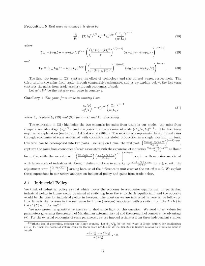
Proposition 5 Real wage in country i is given by

wiPi=�Ti=�

��1=�

L��1i ��1=�ii

��iwiLi

���1(28)

where

�H � (wHLH + wFLF =�)�HH

�(� (ev)! (ev))�

�

�1=(��1)(wHLH=� + wFLF )

!1��HH

(29)

and

�F � (wHLH=� + wFFLF )�FF �

1

� (� (ev)! (ev))��1=(��1)

(wHLH + wFLF =�)

!1��FF: (30)

The �rst two terms in (28) capture the e¤ect of technology and size on real wages, respectively. Thethird term is the gains from trade through comparative advantage, and as we explain below, the last termcaptures the gains from trade arising through economies of scale.Let wAi =P

Ai be the autarky real wage in country i.

Corollary 1 The gains from trade in country i are

wi=PiwAi =P

Ai

= ��1=�ii

��iwiLi

���1(31)

where �i is given by (29) and (30) for i = H and F , respectively.

The expression in (31) highlights the two channels for gains from trade in our model: the gains fromcomparative advantage (��1=�ii ), and the gains from economies of scale ((�i=wiLi)

��1). The �rst termrequires no explanation (see EK and Arkolakis et al (2010)). The second term represents the additional gainsthrough economies of scale associated with concentrating global production in a single location. In turn,

this term can be decomposed into two parts. Focusing on Home, the �rst part,�wHLH+wFLF =�

wHLH

�(��1)�HH

,

captures the gains from economies of scale associated with the expansion of industries wHLH+wFLF =�wHLHat Home

for v � ev, while the second part, �� (�(ev)!(ev))��

��wHLH=�+LF

wHLH

���1�1��HH

, captures those gains associated

with larger scale of industries at Foreign relative to Home in autarky by wHLH=�+wFLFwHLH

for v � ev, with theadjustment term

�(�(ev)!(ev))�

�

�arising because of the di¤erence in unit costs at the cut-o¤ v = ev. We exploit

these expressions in our welare analyses on industrial policy and gains from trade below.

3.1 Industrial Policy

We think of industrial policy as that which moves the economy to a superior equilibrium. In particular,industrial policy in Home would be aimed at switching from the F to the H equilibrium, and the oppositewould be the case for industrial policy in Foreign. The question we are interested in here is the following:How large is the increase in the real wage for Home (Foreign) associated with a switch from the F (H) tothe H (F ) equilibrium?13

We now present a quantitative exercise to shed some light on this question. We need to set values forparameters governing the strength of Marshallian externalities (�) and the strength of comparative advantage(�). For the external economies of scale parameter, we use implied estimates from three independent studies:

13Without loss of generality, consider the Home country. Let wiH=PiH be the real wage in Home country for equilibrium

i = H;F . Then the potential welfare gains for Home from producing all the disputed industries relative to producing none issimply

wHH=PHH � wFH=PFHwFH=P

FH

� 100:

17

Antweiler and Tre�er (2002) general equilibrium approach using data on 71 countries (� = 1:054); Fussand Gupta (1981) analysis using Canadian data (� � 1= (1� �) = 1:15); and Paul and Siegel (1999) partialequlibrium approach using industry level US manufacturing data (� � 1= (1� �) = 1:3). For the comparativeadvantage parameter we use three estimates for � coming from EK, namely 3:6, 8:28 and 12:86.The results are reported in the tables below. Not surprisingly, the set of disputed industries increases

with trade costs, and the trade cost associated with the largest set of disputed industries increases with thescale parameter (recall that we restrict our attention to � = e� , refer to Figure 4 ). In all cases, we computethe trade cost associated with the largest set of disputed industries, e� , and analyze the welfare implications ofthe two extreme equilibria. For symmetric countries, we need only examine the welfare implications of givingall the disputed industries to the Home country. In all other cases we use H and F to indicate whether wewe are considering the equilibrium in which all the disputed goods production go to either Home or Foreignrespectively. Importantly, note that a lower � implies greater variability of productvity across the entire setof industries, and thus stronger forces of comparative advantage. In contrast a higher � implies strongerexternal economies of scale.

Table 1 Gains from Disputed Industries (Symmetric Countries)� 1:05 1:15 1:30� 3:60 8:28 12:86 3:60 8:28 12:86 3:60 8:28 12:86e� 1:04 1:10 1:19Scope Indust. Pol. 0:06% 0:07% 0:07% 0:40% 0:45% 0:46% 1:46% 1:64% 1:69%

Table 1 indicates that there are additional gains from trade associated with producing the entire setof disputed industries and as a result gives us a measure of the potential scope for industrial policy. Themagnitudes of these additional gains range from a negligble 0:06% to at most about 2%, with the potentialimportance increasing strongly with the strength of Marshallian externalities (�), and decreasing weaklywith the strength of comparative advantage (1=�). Essentially, a higher � or a higher � increases the scopefor industrial policy by expanding the set of disputed industries. The former does so by expanding the rangeof low trade costs for which industrial policy applies and as a result raises the low trade cost associated withthe largest set of disputed industries (e�).

Table 2 Home has Superior Technology (TH = 2; TF = 1)� = 12:86; � = 1:30

H FGains from disputed industries 1:48% 1:55%Share of disputed industries 1:36% 1:36%

Might asymmetries alter the basic result above? In Table 2, we explore technology asymmetry by assum-ing the Home country has on average superior technology, and analyze the welfare implications using onlythe highest implied external economies of scale and comparative advantage parameter estimates so as tofocus on the maximum possible scope for industrial policy. The results indicate that the additional welfaregains for both countries do not diverge much from the case of symmetric countries, that is, additional welfaregains of 1:48% for the Home country and 1:55% for the Foreign one, with the disputed industries accountingfor 1:36% of all industries.

Table 3 Home has a Larger Labor Force (LH = 2; LF = 1))� = 12:86; � = 1:30

H FGains from disputed industries 0:70% 1:39%Share of disputed industries 0:66% 0:66%

18

In Table 3, we explore the possibility when one country has a larger labor force. The additional welfaregains from producing the set of disputed industries are approximately two times higher for the small country,1:39% versus 0:70% for the large one (here again we use only the highest Marshallian externalities andcomparative advantage parameter estimates). However, the maximum potential gains are still within therange implied by our benchmark case of symmetric countries.While, in principle, there appears to be a potential role for industrial policy that results from the inde-

terminancy of trade patterns for a set of weak comparative advantage industries in the presence of low tradecosts, quantitatively the scope for such a role appears to be modest.

3.2 The Gains from Trade

In this subsection, we ask: how do Marshallian externalities a¤ect the overall gains from trade? We do adecomposition of gains from trade implied by the expression (31) using the parameter estimates from theprevious section for the case of symmetric countries with low trade costs. Next, we show that the modelreadily extends to a multicountry setting when there are no barriers to trade, and yields interesting insightsregarding the gains from trade.

3.2.1 Decomposition of the Gains from Trade: A First Look

In the previous subsection, we identi�ed two sources of gains from trade: the gains from comparativeadvantage (��1=�ii ); and the gains from external economies of scale ((�i=wiLi)

��1). Also, note that, giventrade shares, accounting for Marshallian externalities imply larger gains from trade over and above thoseof a traditional constant returns framework, which captures only the gains from comparative advantage. Adecomposition of these gains for the case of symmetric countries is reported in Table 4 below. The third rowreports the overall gains from trade in percentage terms14 , whereas the last two rows report the contributionof comparative advantage and Marshallian externalities to the overall gains from trade for the case of lowtrade costs, � = e� .15 We focus on the "natural" equilibrium in which each country produces exactly one halfof the entire set disputed industries, that is, ev = 1=2.Table 4 Gains from Trade (Symmetric Countries with Low Trade Costs)� 1:05 1:15 1:30� 3:60 8:28 12:86 3:60 8:28 12:86 3:60 8:28 12:86e� 1:04 1:12 1:18Total 22:95% 10:27% 7:03% 26:13% 13:68% 10:52% 31:81% 19:29% 16:12%Comp. Adv. 93:19% 85:61% 79:29% 82:95% 65:30% 53:91% 69:72% 47:46% 36:06%Marsh. Ext. 6:81% 14:39% 20:71% 17:05% 34:70% 46:09% 30:28% 52:54% 63:94%

In Table 4 we see that the contribution of external economies of scale to the overall gains from traderanges from approximately 7% (strongest comparative advantage, weakest Marshallian externalities) to 64%(weakest comparative advantage, strongest Marshallian externalities). Interestingly, our middle range es-timates of the two key parameters (� = 8:28, � = 1:18), imply the contribution can be substantial, withMarshallian externalities accounting for roughly 35% of the overall gains from trade of 14%.

3.2.2 Gains from Marshallian Externalities: A Multicountry Framework

In our partial analysis, we have already established that in the absense of trade costs there exists a uniqueequilibrium in which the patterns of specialization are consistent with comparative advantage. In the Ap-pendix we demonstrate that the case of costless trade can be readily generalized to multiple countries in

14 In particular, we compute wi=Pi�wAi =PAi

wAi =PAi

� 100, where wi=Pi is the real wage in the equilibrium with trade and wAi =PAi is

the autarky real wage for country i.15We calculate the contribution of Marshalllian externalities to the overall gains from trade by computing

ln [�i=wiLi](��1)� = ln

�(wi=Pi) =

�wAi =P

Ai

��.

19

which the gains from trade for any country n can be calculated using a simple formula depending only onthe expenditure share on domestically produced goods and the two key parameters governing the strengthof comparative advantage and Marshallian externalities.16 Formally,

Proposition 6 Under frictionless trade, the gains from trade for any country n are

wn=PnwAn =P

An

= ��1=�nn ��(��1)nn : (32)

Here again the �rst term captures the gains from comparative advantage, while the second that fromMarshallian externalities. Equation (32) has an interesting implication. As is consistent with a the standardEK-type model with no economies of scale, the overall gains from trade depend primarily on a country�sexpenditure share on its own goods, and as such can vary across countries. However, a simple decompositionof the gains illustrate that, given trade shares, the contribution of each channel to the total gains from tradeis constant across countries. Formally,

Corollary 2 For any country n, comparative advantage and Marshallian externalities account for shares ofthe overall gains from trade 1

1+(��1)� and(��1)�1+(��1)� , respectively.

Table 5 Gains from Trade (Frictionless Trade)� 1:05 1:15 1:30� 3:60 8:28 12:86 3:60 8:28 12:86 3:60 8:28 12:86Comp. Adv. 84: 75% 70: 72% 60: 86% 64:94% 44:60% 34:14% 48:08% 28:70% 20:59%Marsh. Ext. 15:25% 29:28% 39:14% 35:06% 55:40% 65:86% 51:92% 71:30% 79:41%

Table 5 reports a decomposition of the gains from trade using corollary along with the parameter estimatesfrom the previous subsection. Here the results indicate that Marshallian externalities account for at leastabout 15% and at most approximately 79% of the total gains from trade. Interestingly, the median parameterestimates suggests a contribution of more than a half of the overall gains from trade.

4 Concluding Remarks

In this paper we provide insights to longstanding questions regarding external economies of scale and itsimplications for the patterns of international trade, the gains from trade, and a role for industrial policy.Our paper contributes to the literature by revisiting the implications of trade costs in a new game theoreticframework by GRH designed mainly to overturn the indeterminancy of trade patterns associated with theprevalence of multiple equilibria in the early literature.In the main, we make three points. First, as is consistent with the early literature, we show that

trade patterns are indeterminate for a set of "weak" comparative advantage industries in the presence ofMarshallian externalities and low trade costs. More importantly, we demonstrate that the multiple equilibriaassociated with this set of "disputed" industries implies trade patterns need not be consistent with "natural"comparative advantage. Second, we show that the multiple Pareto-rankable equilibria associated with theset of "disputed" industries also provides a motive for industrial policy. We follow up with a quantitativeexploration of its potential importance. The quantitative evidence suggests modest welfare gains of at mostabout 2%. Finally, our framework allows us to ask whether Marshallian externalities lead to additional gainsfrom trade. Our analysis indicates that this is indeed the case. In particular, using the median parameterestimates, our quantitative results imply that Marshallian externalities can account for approximately 35%of the overall gains from trade.

16One can verify that this case can also be readily extended to more general CES preferences and its associated demand withconstant price elasticity � > 1. The only additional restriction required in this case is � < 1 + ��, where � � � (1� �) + �.

20

A Appendix

A.1 Partial Equilibrium

Pro�ts are increasing in pricesWe have already established that � < 1 is su¢ cient to imply that pro�ts are increasing in the price for a

�rm that sells in a single market. Now consider the case of a �rm that sells in both markets. A Home �rmthat sells at prices pH and pF in Home and Foreign makes pro�ts of

�(pH ; pF ) ��pH �

wHaHA (xH(pH) + xF (pF ))

�xH(pH) +

�pF �

wHaH�

A (xH(pH) + xF (pF ))

�xF (pF ):

Simple di¤erentiation reveals that, �2(pH ; pF ) > 0 if � < 1, but �1(pH ; pF ) > 0 requires a more stringentcondition, namely � < � xH(pH)+xF (pF )

xH(pH)+�xF (pF ). A su¢ cient condition here is that � < 1=�, which is stated above

as Assumption 3.

Proof of Proposition 1. De�ne �MAX � 1=� and �MAX � 1=2 (recall Assumption 1 requires � � 1=2).To prove the existence of e� and �CSH we use two results: �rst, that gH(1) = 1 and gH(�) is increasingfor � > 1, and second that hH(1) > 1 and hH(�) is decreasing for � � 1 with hH(�MAX) < 1. Toprove the �rst result, note that 2g0H(�) = 1 � 1=�2 > 0 implies g0H(�) > 0. To prove the second result,note that @ lnhH(�)

@ ln � = � �1+� � 1. Since � < 1 (Assumption 1), then this is negative. Also, note that

hH(�MAX) = ��1MAX (1 + �MAX)�= � (1 + 1=�)

�. Since � (1 + 1=�)� is increasing in �, to prove thathH(�MAX) < 1 for any � 2 (0; �MAX ] it is su¢ cient to show that �MAX (1 + 1=�MAX)

�MAX < 1. But thisis clearly satis�ed. These two results along with the continuity of both gH(:) and hH(:) imply that thereexists a unique e� which is higher than 1, with gH(e�) > 1. Moreover, for any �! 2 [hH(�MAX); 1) there existsa unique �CSH . Symmetry implies that e� uniquely satis�es gF (�) = hF (�) and gF (e�) < 1. Symmetry alsoimplies that gF (1) = 1 and gF (�) is decreasing for � > 1, and second that hF (1) < 1 and hF (�) is increasingfor � � 1 with hF (�MAX) > 1. One can also verify that there exists a unique � such that hH (�) = hF (�) = 1and � > e� .We now need to establish that for every � the ranges for both cases a and b exist, i.e., hH(�MAX) <

gF (e�) < 1. We have already shown above that the second inequality holds. Hence, we need to show that forevery � we have hH(�MAX) < gF (e�). Recall that hH(�MAX) = �

�1MAX (1 + �MAX)

�= � (1 + 1=�)

� and e�is implicitly de�ned by gF (�) = hF (�) or equivalently 2

1=�+� = � (1 + �)��. So we need to show that for all

� 2 [(0; �MAX ] we have hH(�MAX) < gF (e�) or � (1 + 1=�)� < gF (e�). De�ne e�MAX as that which implicitlysolves 2

1=�+� = � (1 + �)��MAX . Note that � (1 + 1=�)� is increasing in �. Also, note that e� is increasing in

� implies gF (e�) is decreasing in �. Hence, it is su¢ cient to show �MAX (1 + 1=�MAX)�MAX < gF (e�MAX).

One can then readily verify that this is satis�ed. The result then follows, that is, for any � 2 [0; 1=2] thereexists a range for which both case (a), gF (e�) > �! � hH (�MAX), and (b), 1 > �! � gF (e�), apply.The results for cases a and b then follow

Intermediate Trade CostsWe now establish that for any good �! � 1 there exists a range of trade costs for which no pure strategy in

which production is either concentrated in a single country nor one in which there is domestic only productioncan be sustained as an equilibrium. Recall �rst that by Proposition 2 we know that an equilibrium with notrade exists if and only if �! � lH(�). As established above, lH(�) is decreasing and intersects the horizontalline with �! = 1 at point �NTH (1) = 21+� � 1. It is readily veri�ed that �CSH (1) < �NTH (1). To see this

recall that �CSH (1) is de�ned implicitly by 1 = hH(�) � (1+�)�

� . Since hH (:) is strictly decreasing, to show

that �NTH (1) > �CSH (1), it is su¢ cient to show that 1 > (1+�NTH (1))

�

�NTH (1)

() �NTH (1) >�1 + �NTH (1)

��, or

21+� � 1 >�21+�

��. But this is satis�ed for all � < 1=2, a restriction satis�ed by Assumption 1.

We now establish that the curve hH(�) is always below the curve lH(�), so that �CSH (�!) < �NTH (�!).This further implies that for any relevant �! � 1 there is no pure strategy equilibrium for � 2]�CSH (�!); �NTH (�!) [.As mentioned above our analysis is restricted to the range of � that satis�es Assumption 3, i.e., � < 1=�.

21

De�ne �MAX � 1=�. Assumption 2 implies our analysis is relevant for any � 2 [1; �MAX ]. We nowproceed to establish that lH (�) > hH (�) for all � 2

��NTH ; �MAX

�. We do this in three steps: �rst, we �rst

show that lH(�MAX) > hH(�MAX), second, we establish that l0H(�) � h0H(�) � 0 for all � 2 (1; �MAX), andthird, we establish the �nal result using steps one and two.Step 1: Since lH(:) is decreasing then lH(�MAX) > hH(�MAX) is equivalent to 1 < �lH (hH(1=�)), which

in turn is equivalent to

1 <

2

�1 +

�� (1 + 1=�)

��1=(1��)��

� 1�� (1 + 1=�)

��1=(1��)

=�

:

It can be veri�ed that this inequality is satis�ed for 0 � � � 1=2:Step 2: Now we proceed to show that l0H(�) � h0H(�) () jh0H (�)j � jl0H (�)j for all � 2 (1; �MAX).

Totally di¤erentiating2(1+y1=(1��))

��1y1=(1��)

= � , we have

l0H (�) = �(1� �) y�

� � ��1+�y1=(1��)

1+y1=(1��)

�� :Similary, we have h0H (�) = �

�1� �

�1+�

�y. Hence, jh0H (�)j � jl0H (�)j if

1

�� �

1 + �� 1� ��

� � ��1+�y1=(1��)

1+y1=(1��)

��A su¢ cient condition for this is

� � 1

�

which is clearly satis�ed for � = �MAX . The result then follows.Step 3: We now establish that lH (�) > hH (�) for all � 2

��NTH ; �MAX

�. From the analysis above

along with Step 1, we already know that lH(�NTH ) > hH(�NTH ) and lH(�MAX) > hH(�MAX). Suppose by

contradiction there exists � 0 2��NTH ; �MAX

�such that lH(� 0) = hH(� 0). Then l0H(�) � h0H(�) (by Step 2)

along with lH(�NTH ) > hH(�NTH ) implies l(�MAX) < h(�MAX). A contradiction. Hence, the result follows.

Mixed Strategy proposed by GRHGRH propose an equilibrium in which Foreign �rms do not export and charge a price pAF while Home

�rms mix between a local strategy (no export) with pAH and a global pricing strategy, where �rms chargeprice pAF in Foreign and a price p

GH in Home that satis�es �H(p

GH)+�F (p

GH) = 0, where �H(p

GH) and �F (p

GH)

are de�ned in the text. As a �rst step, we show that �F (pGH) < 0, implying that Home �rms make losses inForeign. To see this, let

�(pH ; pF ) ��pH �

wHaH(xH(pH) + xF (pF ))�

�xH(pH) +

"pF �

wHaH�

(xH(pH) + xF (pF ))�

#xF (pF );

and note that �H(pGH) + �F (pGH) = 0 can be written as �(pGH ; p

AF ) = 0. Let�s imagine for a second that

pGH = p0H , where p

0H is de�ned implicitly by

p0H =wHaH

(xH(p0H) + xF (�p0H))

�:

In this case we would have �(p0H ; �p0H) = 0 �if Home �rms charged prices p0H and �p0H then they would

indeed make zero pro�ts. But the violation of condition (5) implies that �p0H > pAF , so charging �p0H in

Foreign cannot be part of an equilibrium. Instead, the proposed strategy is to charge pGH in Home and pAFin Foreign �with pGH = p0H , this means prices p

GH in Home and pAF in Home, leading to pro�ts �(p

0H ; p

AF ).

Our result that pro�ts are increasing in prices (i.e., the best that a deviating �rm can do is to shavecurrent prices) implies that �2 > 0, so �(p0H ; �p

0H) = 0 implies that �(p0H ; p

AF ) < 0. It is easy to see that

22

�(p0H ; pAF ) = �H(p

0H) + �F (p

0H), hence we can conclude that �H(p

0H) + �F (p

0H) < 0. But p

AF < �p

0H implies

that

�(p0H) �"p0H �

wHaH�xH(p0H) + xF (p

AF

�)�

#xH(p

0H) >

�p0H �

wHaH(xH(p0H) + xF (�p

0H))

�

�xH(p

0H) = 0;

hence �H(p0H) > 0. Combined with �H(p0H) + �F (p

0H) < 0, we then conclude that �F (p

0H) < 0. Since p

GH

is de�ned by �(pGH ; pAF ) = 0 then the fact that �1 > 0 implies that p

GH > p0H . But since �

0F < 0, we �nally

conclude that �F (pGH) < 0.As a second step, we show that �F (pGF ) < 0 implies that there exists a pro�table deviation to the proposed

strategy. If the probability of choosing the local strategy is qH , the expected pro�ts made by a Home �rmunder the global strategy are

��H(p

GH) + �F (p

GH)� �qH +

1�qH2

�= 0. Now consider a deviation to a pure

strategy with price in Foreign equal to pAF and the local price just below pGH , say at p0H = pGH � "0. The

pro�ts under the deviation are qH [�H(p0H) + �F (p0H)] + (1� qH) [�H(p0H) + �F (p0H)=2]. Since p0H � pGH

then �H(p0H) + �F (p0H) � 0 and �F (p0H) � ��H(p0H), hence pro�ts under this deviation are close to

(1� qH) �H(p0H)=2, and this is positive. Intuitively, by charging a slightly lower price in the domesticmarket, a Home �rm secures all the pro�ts from Home sales while not incurring more losses in Foreign.

A.2 General Equilibrium

Lemma 1 The functions vgH(�) and vgF (�) exist (this entails existence and uniqueness of a solution in v

to (24) and (26) respectively), vgH(�) is increasing and vgF (�) is decreasing, and for any � > 1 we have

vgH(�) > 1=2 > vgF (�).

Proof of Lemma 1. Recall that vgH(�) and vgF (�) are implicitly de�ned by �(v)=!(v) = gH(!(v); �) and

� (v)! (v) = gF (! (v) ; �). Consider �rst vgH(�). We have gH(!(v); �) =

�+(1=v�1)=�1+1=v�1 = �v + (1� v) =� =

v(� � 1=�) + 1=� , hence �(v)!(v) = gH(!(v); �) is equivalent to

(1=v � 1)�1=� = v(� � 1=�) + 1=� ;

where � � ��= (1 + ��). Both the LHS and RHS are increasing in v (since � > 1=�). To show that thereexists a solution, note that for v = 1=2 we have the RHS > LHS, whereas for v = 1 the LHS is in�nitewhile the RHS is � , so LHS > RHS. This along with the continuity of the LHS and the RHS guaranteesexistence. For uniqueness, note that the derivative of the LHS is

1

�(1=v � 1)�1=��1 1

v2=1

�(1=v � 1)�1=� 1

v (1� v)

while the derivative of the RHS is � � 1=� . Then we require

1

�(1=v � 1)�1=� 1

v (1� v) > � � 1=�

Since both the LHS and the RHS are increasing in v, we know that any point of intersection occurs at v 2(1=2; 1). In fact, any intersection satis�es (1=v � 1)�1=� = v(� � 1=�) + 1=� . Evaluating the LHS derivativeat such an intersection yields

1

�[v(� � 1=�) + 1=� ] 1

v (1� v) =1

� (1� v) (� � 1=�) +1=�

v (1� v)

Clearly,1

� (1� v) (� � 1=�) +1=�

v (1� v) > � � 1=�

establishing uniqueness.Now we proceed to show that vgH(�) is increasing. Note that the RHS, v(� � 1=�) + 1=� , is increasing

in � . This is obvious because the derivative w.r.t. � is v ��1=�2

�(1� v), and since v > 1=2 and � > 1 then

this is positive. The result then follows from the implicit function theorem.

23

The fact that vgF (�) exists, is unique, and is strictly decreasing follows directly from symmetry. Inparticular, symmetry implies vgH (�) = 1� v

gF (�). The result then follows.

Finally, for a given � , it clearly follows that vgH (�) > 1=2 > vgF (�)

Let e� be de�ned implicitly by vgH (e�) = vhH (e�). Note that if vgH (e�) = vhH (e�) then by symmetry we havevgF (e�) = vhF (e�). Then it is easy to see that for � � e� any CSA ev 2 [vgF (�); vgH(�)] is also a CSE. Thisfollows because for � � e� we have vgH (�) < vhH (�) and vgF (�) > vhF (�), hence conditions (10) and (12) implyconditions (11) and (13). Before establishing this, we �rst establish the existence of vhH(�) and v

hF (�).

Lemma 2 The functions vhH(�) and vhH (�) exist (this entails existence and uniqueness of a solution in v to

(25) and (27)), vhH(�) is decreasing and vhF (�) is increasing in � .

Proof of Lemma 2. Consider �rst vhH(�). Since hH (! (v) ; �) � 1�

h�+(1=v�1)(1=v�1)

i(��1)=�= 1

�

h1 + �v

1�v

i�,

the fact that vhH(�) is implicitly de�ned by �(v)!(v) = hH(!(v); �) is equivalent to vhH(�) being implicitly

de�ned by

(1=v � 1)�1=� = 1

�

�1 +

�v

1� v

��or

v

(1� v)1���

!1=�=1

�[(� � 1) v + 1]�

Both the LHS and RHS are increasing in v (since � > 1 and �� < 1). To show that there exists a solution,note that for v = 0 we have the RHS > LHS, whereas for v = 1 the LHS is in�nite while the RHSis 1=�1��, so LHS > RHS. This along with the continuity of both the LHS and the RHS guaranteesexistence. For uniqueness, note that the derivative of the LHS is

1

�

v

(1� v)1���

!1=�1

v

1� ��v1� v

while the derivative of the RHS is

�1

�[(� � 1) v + 1]� � � 1

(� � 1) v + 1

Then we require

1

�

v

(1� v)1���

!1=�1

v

1� ��v1� v > �

1

�[(� � 1) v + 1]� � � 1

(� � 1) v + 1

Any intersection satis�es�

v(1�v)1���

�1=�= 1

� [(� � 1) v + 1]�. Evaluating the LHS derivative at such an

intersection implies we require

1

�

1

�[(� � 1) v + 1]� 1

v

1� ��v1� v > �

1

�[(� � 1) v + 1]� � � 1

(� � 1) v + 1

or1

�

1

�

1

v

1� ��v1� v > �

� � 1�

1

(� � 1) v + 1which is clearly satis�ed. Uniqueness then follows.Now we proceed to show that vhH(�) is decreasing. Note that the RHS,

1� [(� � 1) v + 1]

�, is decreasingin � . The result then follows from the implicit function theorem.The fact that vhF (�) exists, is unique, and is increasing follows directly from symmetry. In particular,

symmetry implies vhH (�) = 1� vhF (�). The result then follows

Proof of Proposition 4. Note that the implicit function vgH (�) and vgF (�) characterize the limiting goods

for which the global-deviation condition for both Home and Foreign are satis�ed respectively, while (25) and

24

(27) capture the limiting goods for which the local-deviation condition is also satis�ed. Consider �rst Homecountry. Recall that vhH (�) is the implicit function which solves

(1=v � 1)�1=� = 1

�

��v

1� v + 1��

where � = ��= (1 + ��) and � = (�� 1) =�.Also, recall that vgH (�) is the implicit function which solves

(1=v � 1)�1=� = �v + 1� v�

:

We proceed as follows. First, we establish the existence of a unique b� satisfying vhH (b�) = 1=2. Second,we show that �MAX > b� . Third, we show there exists a unique e� satisfying vgH (e�) = vhH (e�) and e� < b� .Finally, we establish that for the relevant range of trade costs, any CSA within the two extreme cases is alsoa CSE.Note that to show there exists a unique b� satisfying vhH (b�) = 1=2 is equivalent to establishing there exists

a unique b� satisfying � = [� + 1]�. But this follows from Assumption 1 (� � 1=2). To show that �MAX > b� ,it su¢ cient to show that �MAX > b�MAX where �MAX implicitly solves � = [� + 1]�MAX . But this is clearlysatis�ed. The fact that b� also satis�es vhH (b�) = vhF (b�) = 1=2 follows directly from symmetry. In particular,symmetry implies vgH (�) = 1� v

gF (�). The result then follows.

Evaluating the �rst and second equations above at � = 1 yields�vhH=

�1� vhH

��1=�=�vhH=

�1� vhH

�+ 1��

and (vgH= (1� vgH))

1=�= 1 respectively. Since

�vhH=

�1� vhH

�+ 1��> 1, we have vhH (1) > vgH (1) = 1=2.

Also, vgH (1) = 1=2 and vgH (:) strictly increasing (by lemma 1) imply vgH (b�) > 1=2. So we have vgH (b�) >

vhH (b�) = 1=2. Since, both vhH (:) and vgH (:) are continuous there exists e� and e� < b� . Uniqueness follows

from dvgH(�)

d� > 0 (by lemma 1) and dvhH(�)d� < 0 (by lemma 2). The fact that e� also satis�es vgF (e�) = vhF (e�)

and vhF (�) < vgF (�) for any � < e� follows directly from symmetry. In particular, symmetry implies vgH (�) =

1� vgF (�). The result then follows.We now proceed to show that for any � � e� , any allocation ev 2 [vgF (�) ; vgH (�)] with e! � !(ev) is a CSE,

i.e., it satis�es (10)-(13). In particular, ev satis�es � (ev) e! � gH (e!; �) ; � (ev) e! � hH (e!; �) ; � (ev) e! � gF (e!; �)and � (ev) e! � hF (e!; �). Consider the �rst of these conditions: � (ev) e! � gH (e!; �). In lemma 1, we showedthat at v = 1=2 we have RHS > LHS and there exists a unique intersection at v = vgH(�). So for v � v

gH(�)

we must have RHS � LHS, i.e., � (v)!(v) � gH (!(v); �) for any 1=2 � v � vgH(�). Moreover, the fact thatboth the LHS and RHS are strictly increasing and continuous on [0; 1) implies for any 0 � v � vg(�) itmust also be the case that � (v)!(v) � gH (!(v); �). Similarly, symmetry implies for any 1=2 � v � vgF (�)we have � (v)!(v) � gF (!(v); �) and by extension this is also the case for any 0 � v � vgF (�). Hence, forany ev 2 [vgF (�) ; vgH (�)], we have e!�1gF (e!; �) � � (ev) � e!�1gH (e!; �).Consider now, the �rst local-deviation condition: �(v)!(v) � hH(!(v); �). We know that vhH(�) is

implicitly de�ned by

(1=v � 1)�1=� = 1

�

�1 +

�v

1� v

��For v = 1=2 we have LHS is 1, while the RHS is 1� [1 + � ]

�. So for the relevant range of low trade costs alongwith the restriction � < 2, we have RHS > LHS. Moreover, from lemma 2 there exists a unique intersectionat v = vhH(�). Hence, for any v � vhH (�) we have RHS � LHS implies that �(v)!(v) � hH(!(v); �) for any1=2 � v � vhH(�). Similarly, symmetry implies for any 1=2 � v � vhF (�) we have � (v)!(v) � hF (!(v); �).Furthermore, for any � � e� , we have already established that vhH (�) � vgH (�) � 1=2 � vgF (�) � vhF (�). Thus,for any ev 2 �vhH (�) ; vgH (�)�, we have e!�1hF (e!; �) � e!_1gF (e!; �) � � (ev) � e!�1gH (e!; �) � e!�1hH (e!; �).So by de�nition 2, ev is a CSE.Finally, we have already established that there exists a unique solution to vhH (b�) = 1=2. Moreover, since

vgH(�) is increasing and vgH(1) = 1=2 then with e� de�ned by vgH(�) = vhH(�) we must have that b� > e� ,

and vgH (�) > vhH (�) for � 2 (e� ;b� ]. Symmetry implies the corresponding result, i.e., for any � 2 (e� ;b� ],vgF (�) < v

hF (�). Also note that we have already established above that for � � e� and vgH (�) � ev � vgF (�)

we have e!�1gF (e!; �) � � (ev) � e!�1gH (e!; �). By lemma 1, we see that this also applies for any � > 1.

25

Similarly, for any � � e� and vhH (�) � ev � vhF (�) we already know that e!�1hF (e!; �) � � (ev) � e!�1hH (e!; �).That this also applies for any � � b� follows from lemma 2 and the fact that for any � � b� we havevhH (�) � 1=2 � vhF (�). Moreover, for any � 2 (e� ;b� ], we have vgH (�) � vhH (�) � 1=2 � vhF (�) � vgF (�).Hence, for any � 2 (e� ;b� ] and ev 2 �vhF (�) ; vhH (�)�, we have vgH (�) � vhH (�) � ev � vhF (�) � v

gF (�) impliese!�1gF (e!; �) � e!�1hF (e!; �) � � (ev) � e!�1hH (e!; �) � e!�1gH (e!; �). The fact that ev is a CSE then follows

from de�nition 2

A.3 Welfare

A.3.1 Real Wages and the Gains from Trade

Proof of Proposition 5. Allowing for asymmetries in technology and labor force across countries, we canderive a more general version of the relative productivity function, i.e.

� (v) =

�TFTH

�1=�� �v

1� v

�1=��: (33)

Let l � LH=LF . Note also that the more general versions of the global-deviation conditions imply:

gH (!; �) � �+(!l)�1=�

1+(!l)�1; and gF (!; �) � 1+(!l)�1

1=�+(!l)�1�. Using (33), we can rewrite (24) and (26) so that

each is implicitly solved by vH and vF , respectively. Importantly, note that vH and vF are also the shareof goods that Home �rms produce in the extreme cases in which all the disputed industries are allocated tothe Home and Foreign country respectively. Mote that (33) implies

ev = TH

TH + TF���� : (34)

From Proposition 4 we know that the set of equilibria is given by ev 2 [vgF (�); vgH(�)]. In particular, theneccessary global-deviation conditions for complete specialization are satis�ed, that is, ! (ev)�1 gF (! (ev) ; �) �� (ev) � ! (ev)�1 gH (! (ev) ; �).17 Consider �rst the Home country. Then (34) along with �HH = ev implies

�HH =THw

���H

�H(35)

where �H =hTHw

���H + TFw

���F (� (ev)! (ev))���i.

Let pni (v) be the price of good v if i sells to n (i; n = H;F ). Note that since we consider only completespecialization, any country which sells the good supplies the world market. Hence, for any industry v wehave either price pairs18

pHH =wHaH

[xH (pHH) + xF (�pHH)]�and pFH = pHH�

orpFF =

wFaF

[xH (�pFF ) + xF (pFF )]�and pHF = pFF �

where xH(p) = wHLHp and xF (p) = wFLF

p .

17 In our quantitative exercise we also verify that no Home or Foreign �rms have an incentive to target their domestic marketonly, i.e. the local deviation conditions for complete specialization are also satis�ed. Both provide a su¢ cient condition for theexistence of a complete specialization equilibrium.18 In particular, the relevant prices are

pHH (v) =(wHaH (v))

�

(wHLH + wFLF =�)(��1) =

1

zH (v)

(wH)�

(wHLH + wFLF =�)(��1)

and

pFF (v) =(wF aF (v))

�

(wHLH=� + wFLF )(��1) =

1

zF (v)

(wF )�

(wHLH=� + wFLF )(��1) :

26

The associated price index for Home is then given by19

PH = � (�H)�(��1)

(�H)�1=� (36)

where � = e� =�, is Euler�s constant, and

�H � (wHLH + wFLF =�)�HH

�(� (ev)! (ev))�

�

�1=(��1)(wHLH=� + wFLF )

!1��HH

(36) implies �H = (PH=�)��(�H)

�(��1)�. Substituting into (35) yields real wages

wHPH

=�TH=�

��1=�

��1=�HH

��HwH

�(��1):

Analagously, we can derive real wages in Foreign

Proof of Corollary 1. In autarky,

wAHPAH

=�TH=�

��1=�

(LH)(��1)

:

Therefore, gains from trade arewH=PHwAH=P

AH

= ��1=�HH

��HwHLH

�(��1):

Similarly, we can also derive the gains from trade in Foreign

A.3.2 Multiple Countries and Frictionless Trade

We already know that with frictionless trade there exists a unique equilibrium in which the patterns oftrade are consistent with "natural" comparative advantage. The di¤erence here is that we consider K � 2countries. Here K can be large, but �nite. As noted in our general environment, preferences are uniformCobb-Douglas with its associated demand

xi(v) =Dipi (v)

(37)

where Di is aggregate expenditure by country i.The stability condition in (2) holds, namely�

�� 1�

�< 1

and �rms in each industry engage in Bertrand competition on the world market. Before proceeding to theproof we �rst formally restate the de�nition of an equilibrium.

De�nition 3 Given country size Li and country speci�c productivity distribution Fi (z), an equilibrium withfrictionless trade consists of prices pni (v), wi, and quantities xi (v) such that: (a) industry markets clear; (b)�rms in each industry engage price competition in all markets simultaneously; and (c) labor market clears.

19To see this note �rst that

PH = exp

8<:evZ0

ln pHH (v) dv +

1Zevln pHF (v) dv

9=; :Using

pHH (v) =(wHaH (v))

�

(wHLH + wFLF =�)(��1) =

1

zH (v)

(wH)�

(wHLH + wFLF =�)(��1)

and

pFF (v) =(wF aF (v))

�

(wHLH=� + wFLF )(��1) =

1

zF (v)

(wF )�

(wHLH=� + wFLF )(��1)

along with (20), we can derive the price index as noted in (36).

27

Proof of Proposition 6. Price competition amongst �rms in any domestic industry implies average costpricing, that is

pni (v) =wi

zi (v)1=�

Xi (v)(��1)=� (38)

Note that if country i supplies the world market, then Xi (v) =KPn=1

xn (pni (v)) =KPn=1

Dn

pni(v). Moreover, the

actual prices paid for good v is the lowest from all sources i

pn (v) = min fpni (v) ; i = 1; :::;Kg (39)

Complete specialization along with industry market clearing imply

pni (v) =w�i

zi (v)

�KPk=1

wkLkwi

���1 :Using the assumption that the productivity distrbution is Fretchet, we can derive the distribution of pricesthat i presents to20 n

Gni(p) = 1� e�Tiw���i

KPk=1

wkLk

!(��1)�

p�

: (40)

From (40) we can derive the price distribution for which country n actually buys some good j, that is, thelowest price of a good in country n will be less than p unless each source�s price is greater than p

Gn(p) = 1��Ki=1 [1�Gni(p)]

SoGn(p) = 1� e��np

�

where �n =KPi=1

Tiw���i

�KPk=1

wkLk

�(��1)�

.

Hence, the probability n buys from i is given by

�ni = Pr [pni � minfpns : s 6= ig]

=1R0

�s 6=i [1�Gns(p)] dGni(p)

So

�ni =

Tiw���i

�KPk=1

wkLk

�(��1)�

�n=

Tiw���i

KPi=1

Tiw���i

With costless trade �ni is the same for all n, and is also independent of v. Hence, �ni is also the share ofgoods that any country n buys from country i. Moreover, the price of a good country n actually buys fromi has the distribution Gn(p) so that �ni is also the share of expenditure by n on goods produced in i, that is

�ni =XniXn

=

Tiw���i

�KPk=1

wkLk

�(��1)�

�n=

Tiwi���P

k2�Tkwk���

(41)

20 In autarky the distribution of prices is given by Gn(p; fng) = 1� e�Tnwn���(wnLn)(��1)�p� . Hence, it depends not onlyon the state of country n�s technology discounted by its input cost as in EK, but also, because of external economies, on themarket size of n.

28

Also, the associated price index for isPn = ��

�1=�n (42)

where � = e� =� and is Euler�s constant.In equilibrium, labor market clearing/trade balance implies

wiLi =KPn=1

�niXn (43)

Equation (41) along with (43) yield an expression for relative wages

wiwn

=

�Ti=LiTn=Ln

�1=(1+��)(44)

Using (41) and (42) we can derive real wages

wnPn

=�Tn=�

��1=�

L��1n ��1=�nn

�KPk=1

wkLkwnLn

���1In autarky real wage is given by

!An �wAnPAn

=�Tn=�

��1=�

L��1n

Hence, gains from trade arewn=PnwAn =P

An

= ��1=�nn

�KPk=1

wkLkwnLn

���1:

Finally, both (41) and (44) imply

�nn =KPk=1

wnLnwkLk

:

The result then follows

Proof of Corollary 2. From (32) we can then simply derive the contribution of comparative advantage and

Marshallian externalities usingln(��1=�nn )

ln���1=�nn �

�(��1)nn

� and ln(��(��1)nn )ln���1=�nn �

�(��1)nn

� respectively. The result then follows

29

References

[1] Antweiler, Werner, and Daniel Tre�er, "Increasing Returns and All That: A View from Trade," Amer-ican Economic Review, 92 (2002), 93-119

[2] Arkolakis, Costas, Arnaud Costinot, and Andrés Rodríguez-Clare, "New Trade Models, Same OldGains?," forthcoming American Economic Review.

[3] Caballero, Ricardo J., and Richard K. Lyons, "The Role of External Economies in U.S. Manufacturing,"NBER Working Paper No. 3033, 1989.

[4] � , "Internal versus External Economies in European industry," European Economic Review, 34 (1990),805-826.

[5] � , "The Case for External Economies," in Political economy, growth, and Business cycles, A. Cukier-man, Z. Hercowitz, and L. Leiderman, eds. (Cambridge, MA: MIT Press, 1992).

[6] Chan, Vei-Lin, Been-Lon Chen, and Kee-Nam Cheung, "External Economies in Taiwan�s ManufacturingIndustries," Contemporary Economic Policy, 13 (1995), 118-130.

[7] Chipman, John S., "A Survey of the Theory of International Trade: Part 2, The Neo-Classical Theory,"Econometrica, 33 (1965), 685-760.

[8] � , "External Economies and Competitive Equilibrium," Quarterly Journal of Economics, 84 (1970),347-363.

[9] Dornbusch, Rudiger, Stanley Fischer, and Paul Samuelson, "Comparative Advantage, Trade, and Pay-ments in a Ricardian Model with a Continuum of Goods," American Economic Review, 67 (1977),823-839.

[10] Eaton, Jonathan, and Samuel Kortum, "Technology, Geography and Trade," Econometrica, 70 (2002),1741-1779.

[11] Ethier, Wilfred J., "Decreasing Costs in International Trade and Frank Graham�s Argument for Pro-tection," Econometrica, 50 (1982a), 1243-1268.

[12] � , "National and International Returns to Scale in the Modern theory of International Trade,"AmericanEconomic Review, 73 (1982b), 389-405.

[13] Fuss, Melvyn A., and Vinod K. Gupta, "A Cost Function Approach to the Estimation of MinimumE¢ cient Scale, Returns to Scale, and Suboptimal Capacity with an Application to Canadian Manufac-turing," European Economic Review, 15 (1981), 123-35.

[14] Graham, Frank D., "Some Aspects of Protection Further Considered," Quarterly Journal of Economics,37 (1923), 199-227.

[15] Grossman, Gene M., and Esteban Rossi-Hansberg, "External Economies and International Trade: Re-dux," Quarterly Journal of Economics, 125 (2010), 829-858.

[16] Helpman, Elhanan, and Paul R. Krugman, Market Structure and Foreign Trade: Increasing Returns,Imperfect Competition, and the International Economy (Cambridge, MA: MIT Press, 1985).

[17] Henriksen, Espen R., frode steen, and Karen-Helene Ulltveit-Moe, "Economies of Scale in EuropeanManufacturing revisited," Center for Economic Policy Research Discussion Paper No. 2896, 2001.

[18] Kemp, Murray C., The Pure Theory of International Trade and Investment (Englewoods Cli¤s, NJ:Prentice Hall, 1964).

[19] Krugman, Paul R., "Increasing Returns, Imperfect Competition, and the Positive Theory of Interna-tional Trade," in Handbook of International Economics, Vol. 3, G.M. Grossman and K. Rogo¤, eds.(Amsterdam: North-Holland, 1995).

30

[20] � , "Increasing Returns in a Comparative Advantage World," Princeton mimeo, Nov. 2009.

[21] Markusen, James R., and James R. Melvin, "Trade, Factor Prices, and the Gains from Trade withIncreasing Returns to Scale," Canadian Journal of Economics, 3 (1969), 389-402.

[22] Marshall, Alfred, Principles of Economics (London: Macmillan, 1890).

[23] Matsuyama, Kiminori, "Increasing Returns, Industrialization, and Indeterminacy of Equilibrium,"Quarterly Journal of Economics, 106 (1991), 617-650.

[24] Mathews, R.C.O., "Reciprocal Demand and Increasing Returns," Review of Economic Studies, 37 (1949-1950), 149-158.

[25] Melvin, James R., "Increasing Returns to Scale as a Determinant of Trade," Canandian Journal ofEconomics, 3 (1969), 389-402.

[26] Ohlin, Bertil, Interregional and International Trade (Cambridge, MA: Harvard University Press, 1933).

[27] Paul, Catherine J., and Donald S. Siegel, "Scale Economies and Industry Agglomeration Externalities:A Dynamic Cost Function Approach," American Economic Review, 89 (1999), 272-290.

[28] Segoura, Io, "Return to Scale and External Economies: Empirical Evidence from Greek Two-DigitManufacturing Industries," Applied Economic Letters, 5 (1998), 485-490.

[29] Venables, Anthony J., "Tari¤s and Subsidies with Price Competition and Integrated Markets: TheMixed-Strategy Equilibria," Oxford Economic Papers, 46 (1994), 30-44.

31