182
Martin Isenburg University of North Carolina at Chapel Hill Triangle Fixer: Edge-based Connectivity Compression
| Date post: | 20-Dec-2015 |
| Category: |
Documents |
| View: | 219 times |
| Download: | 0 times |

Martin Isenburg
University of North Carolina at Chapel Hill
Triangle Fixer:
Edge-based Connectivity Compression
Introduction
A new edge-based encoding schemefor polygon mesh connectivity.

Introduction
A new edge-based encoding scheme
for polygon mesh connectivity.
compact mesh representations

Introduction
A new edge-based encoding scheme
for polygon mesh connectivity.
compact mesh representations simple implementation
Introduction
A new edge-based encoding scheme
for polygon mesh connectivity.
compact mesh representations simple implementation fast decoding
Introduction
A new edge-based encoding scheme
for polygon mesh connectivity.
compact mesh representations simple implementation fast decoding
Introduction
A new edge-based encoding scheme
for polygon mesh connectivity.
compact mesh representations simple implementation fast decoding
extends to non-triangular meshes

Introduction
A new edge-based encoding scheme for polygon mesh connectivity.
compact mesh representations simple implementation fast decoding
extends to non-triangular meshes extends to meshes with group or triangle strip information
What are ‘Polygon Meshes’ . . . ?
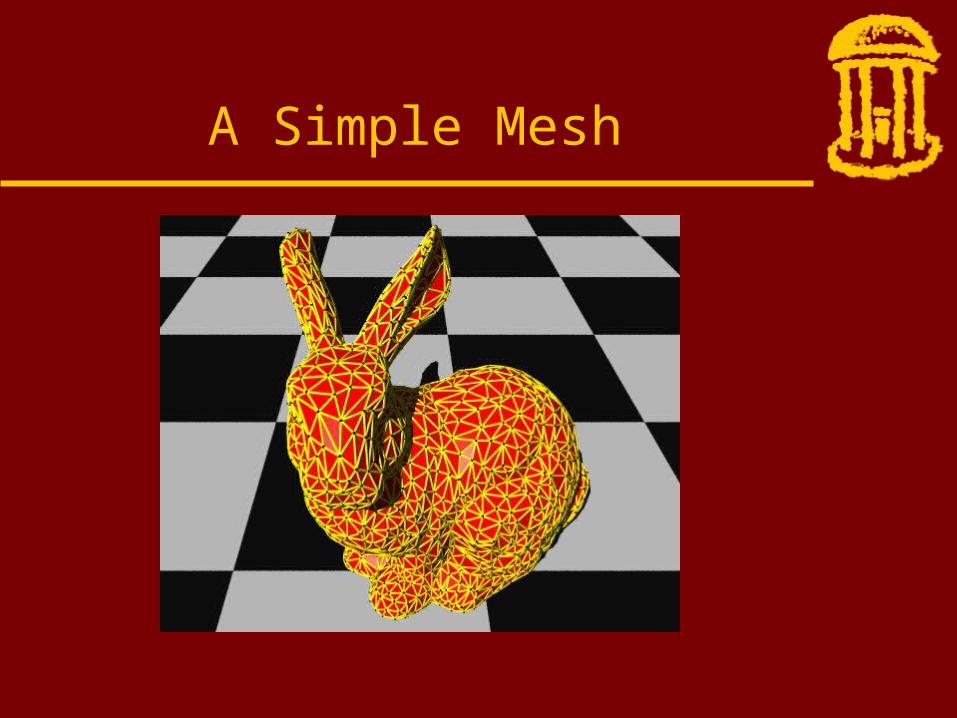
A Simple Mesh

Mesh with Holes
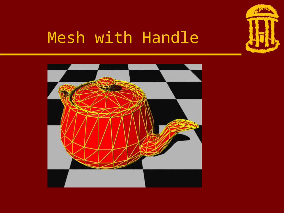
Mesh with Handle
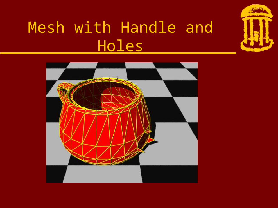
Mesh with Handle and Holes

How are Polygon Meshes stored . . . ?
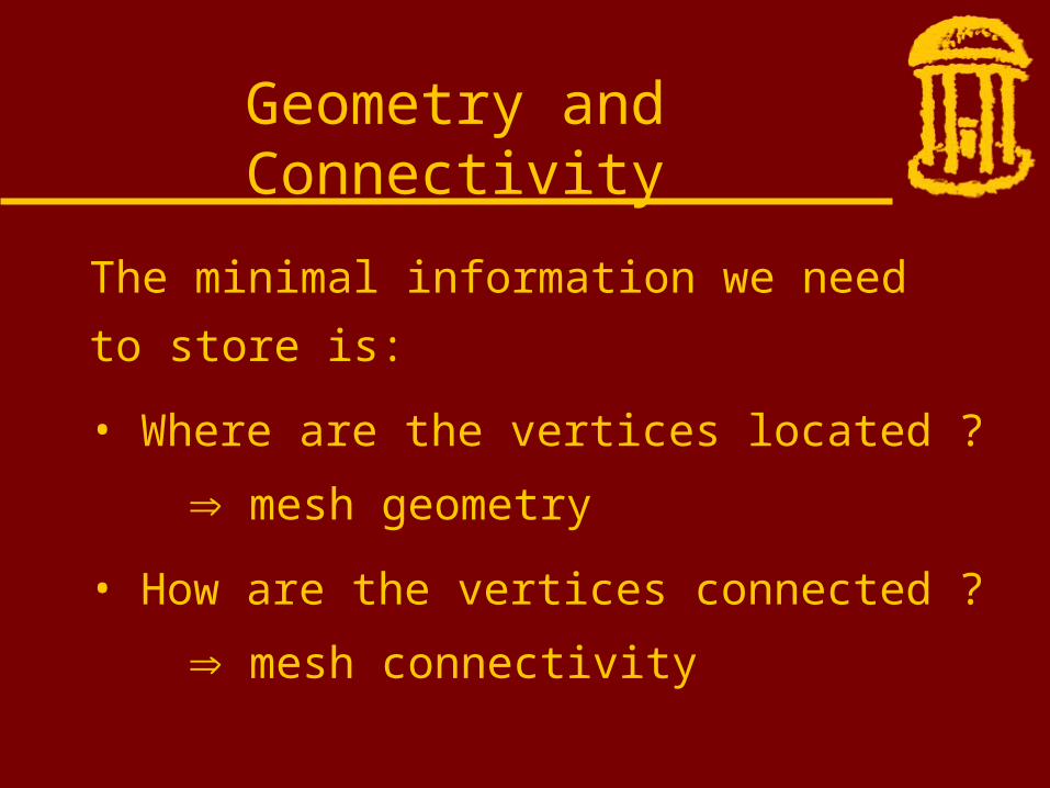
The minimal information we need to
store is:
• Where are the vertices located ?
mesh geometry
• How are the vertices connected ?
mesh connectivity
Geometry and Connectivity

list of vertices x0 y0 z0
x1 y1 z1
x2 y2 z2
x3 y3 z3
4 x4 y4 z4
6 4 . . . . .xn yn zn
Standard Representation

list of vertices list of faces x0 y0 z0 1 4 20
x1 y1 z1
x2 y2 z2
x3 y3 z3
4 x4 y4 z4
6 4 . . . . .xn yn zn
Standard Representation
list of vertices list of faces x0 y0 z0 1 4 20
x1 y1 z1
x2 y2 z2
x3 y3 z3
4 x4 y4 z4
6 4 . . . . .xn yn zn
Standard Representation

list of vertices list of faces x0 y0 z0 1 4 20
x1 y1 z1
x2 y2 z2
x3 y3 z3
4 x4 y4 z4
6 4 . . . . .xn yn zn
Standard Representation
list of vertices list of faces x0 y0 z0 1 4 20
x1 y1 z1
x2 y2 z2
x3 y3 z3
4 x4 y4 z4
6 4 . . . . .xn yn zn
Standard Representation

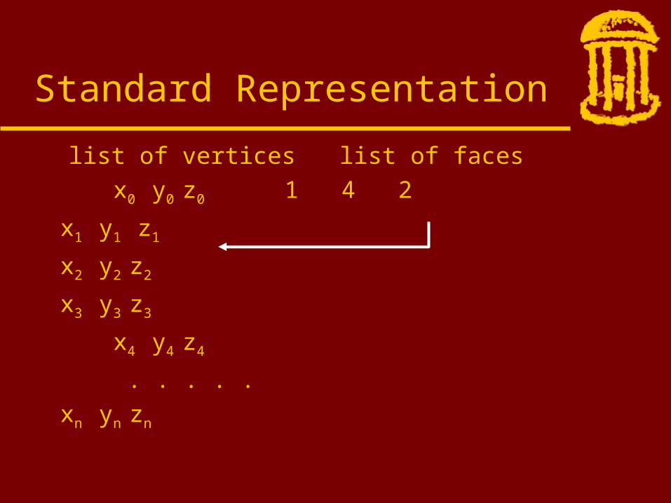
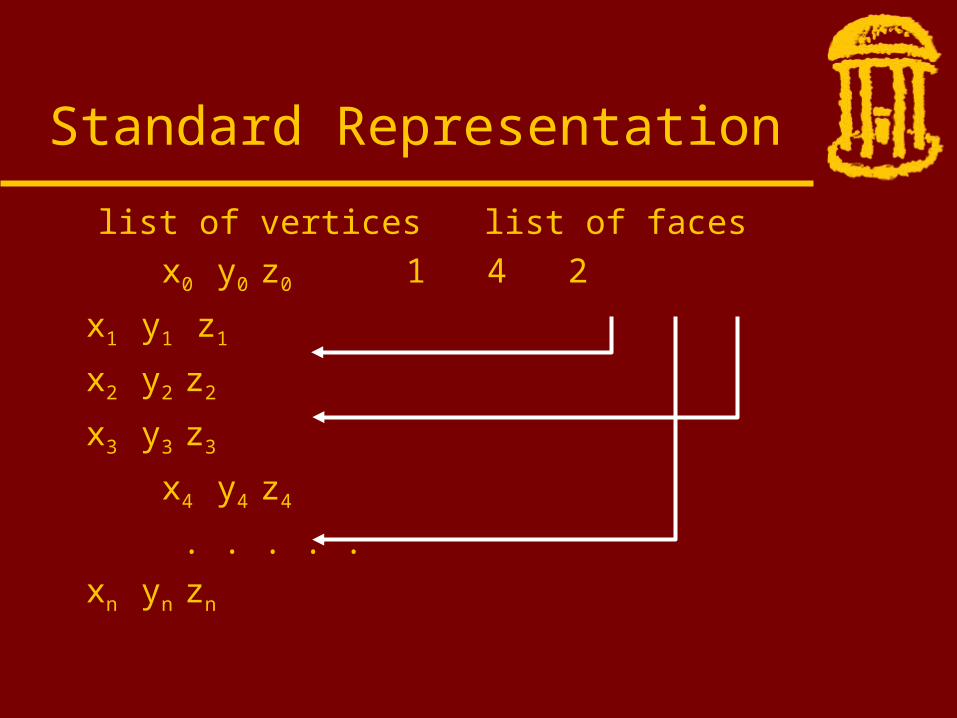
list of vertices list of faces x0 y0 z0 1 4 2
x1 y1 z1 2 3 0 3 4
x2 y2 z2 u2 v2 w2 4 0 5 3 4
x3 y3 z3 u3 v3 w3 3 4 5 3 6
4 x4 y4 z4 u4 v4 w4 5 0 2
. . . . .xn yn zn
. . . . .
. . . . .
. . . . .
Standard Representation
list of vertices list of faces x0 y0 z0 1 4 2
x1 y1 z1 2 3 0 3 4
x2 y2 z2 u2 v2 w2 4 0 5 3 4
x3 y3 z3 u3 v3 w3 3 4 5 3 6
4 x4 y4 z4 u4 v4 w4 5 0 2
. . . . .xn yn zn
. . . . .
. . . . .
. . . . .
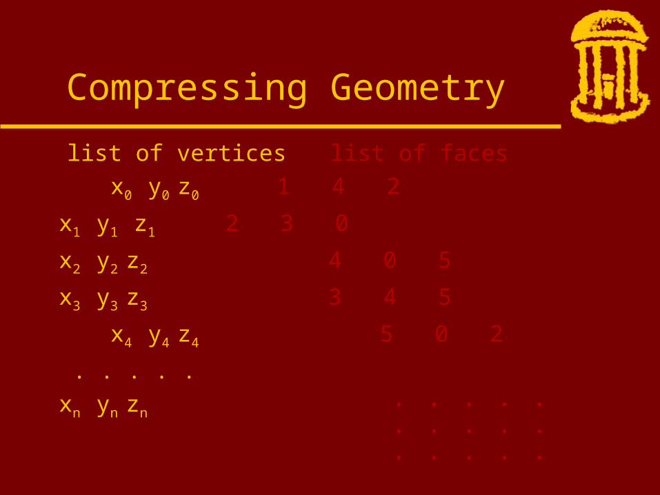
Compressing Geometry

list of vertices list of faces x0 y0 z0 1 4 2
x1 y1 z1 2 3 0 3 4
x2 y2 z2 u2 v2 w2 4 0 5 3 4
x3 y3 z3 u3 v3 w3 3 4 5 3 6
4 x4 y4 z4 u4 v4 w4 5 0 2
. . . . .xn yn zn
. . . . .
. . . . .
. . . . .
Compressing Connectivity

0
1
10
2
3
45
6
7
8
9
1112
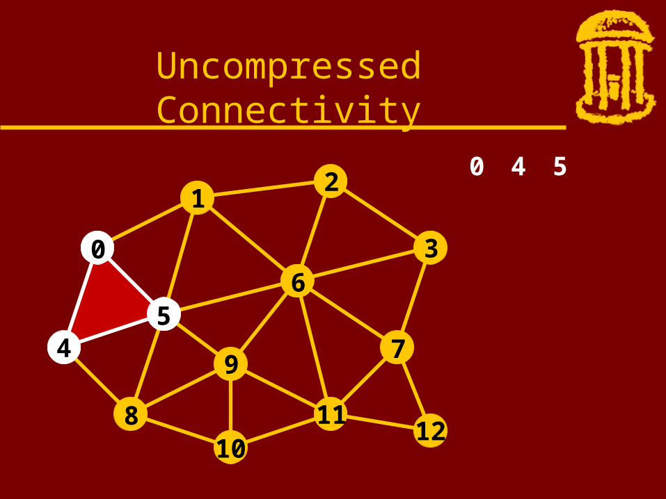
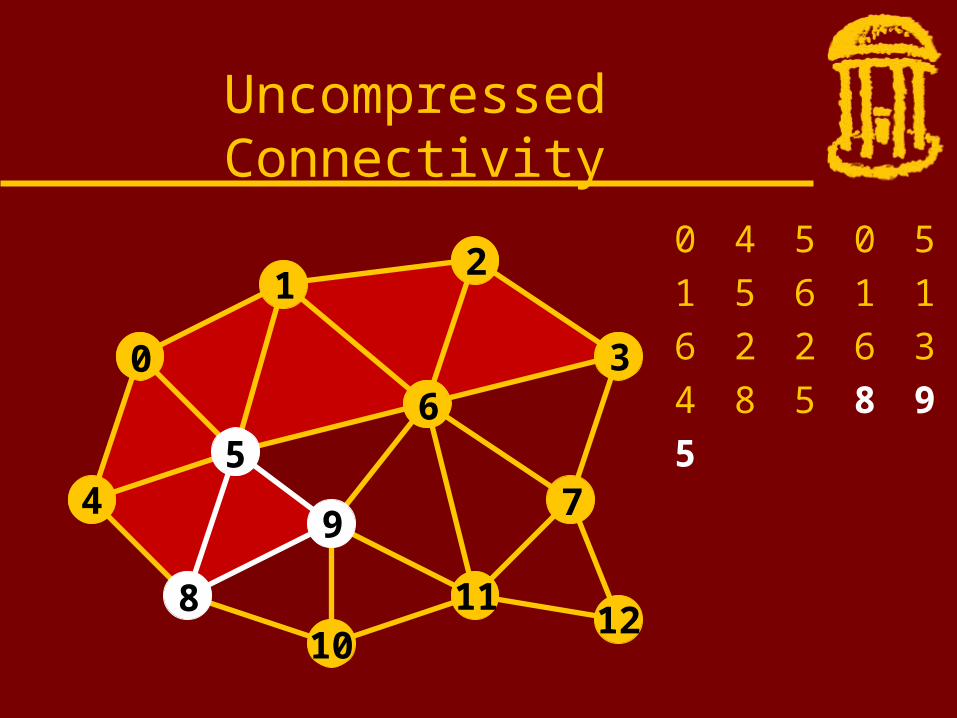
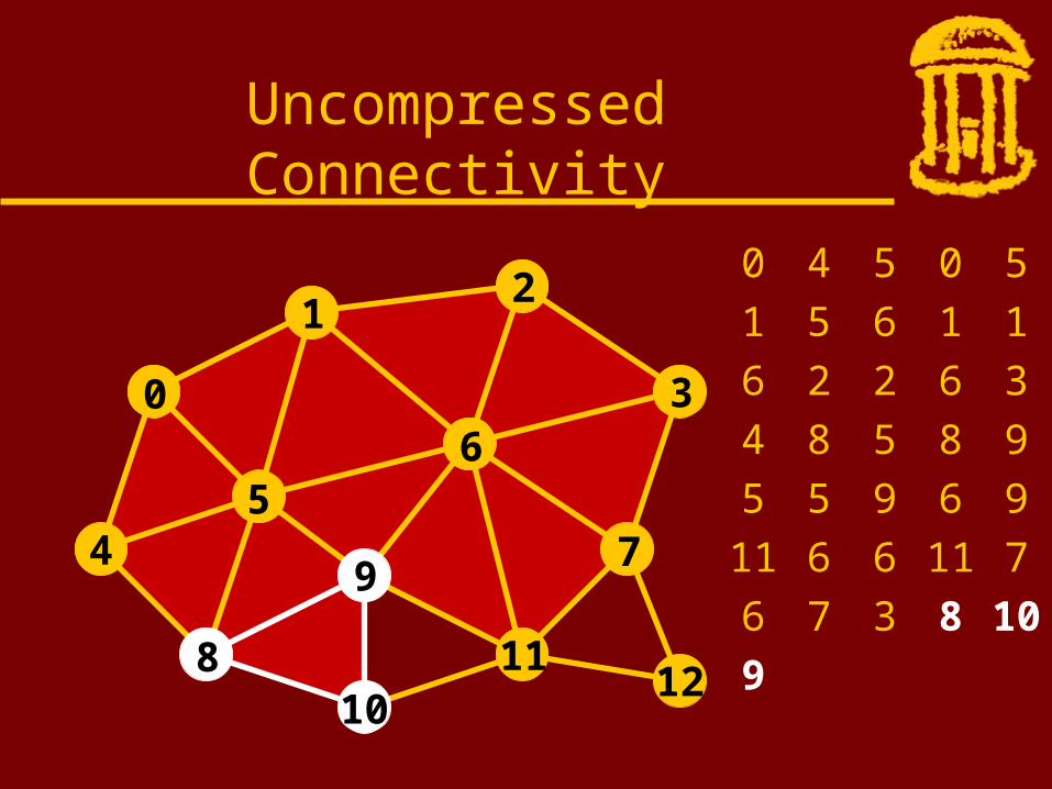
Uncompressed Connectivity
0
1
10
2
3
45
6
7
8
9
1112
0 4 5
Uncompressed Connectivity

0
1
10
2
3
45
6
7
8
9
1112
0 4 5 0 5
1
Uncompressed Connectivity
0
1
10
2
3
45
6
7
8
9
1112
0 4 5 0 5
1 5 6 1
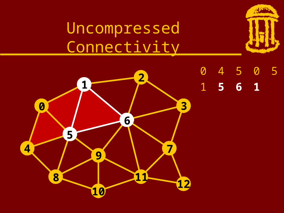
Uncompressed Connectivity
0
1
10
2
3
45
6
7
8
9
1112
0 4 5 0 5
1 5 6 1 1
6 2
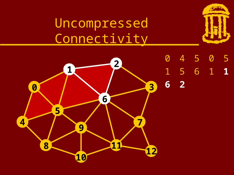
Uncompressed Connectivity
0
1
10
2
3
45
6
7
8
9
1112
0 4 5 0 5
1 5 6 1 1
6 2 2 6 3
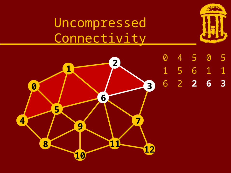
Uncompressed Connectivity

0
1
10
2
3
45
6
7
8
9
1112
0 4 5 0 5
1 5 6 1 1
6 2 2 6 3
4 8 5
Uncompressed Connectivity
0
1
10
2
3
45
6
7
8
9
1112
0 4 5 0 5
1 5 6 1 1
6 2 2 6 3
4 8 5 8 9
5
Uncompressed Connectivity

0
1
10
2
3
45
6
7
8
9
1112
0 4 5 0 5
1 5 6 1 1
6 2 2 6 3
4 8 5 8 9
5 5 9 6
Uncompressed Connectivity
0
1
10
2
3
45
6
7
8
9
1112
0 4 5 0 5
1 5 6 1 1
6 2 2 6 3
4 8 5 8 9
5 5 9 6 9
11 6
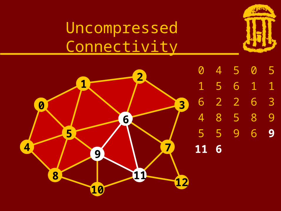
Uncompressed Connectivity
0
1
10
2
3
45
6
7
8
9
1112
0 4 5 0 5
1 5 6 1 1
6 2 2 6 3
4 8 5 8 9
5 5 9 6 9
11 6 6 11 7
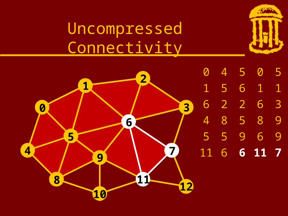
Uncompressed Connectivity
0
1
10
2
3
45
6
7
8
9
1112
0 4 5 0 5
1 5 6 1 1
6 2 2 6 3
4 8 5 8 9
5 5 9 6 9
11 6 6 11 7
6 7 3
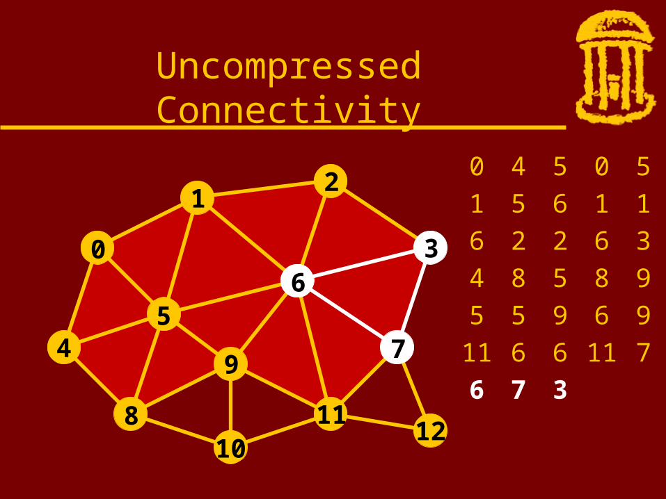
Uncompressed Connectivity
0
1
10
2
3
45
6
7
8
9
1112
0 4 5 0 5
1 5 6 1 1
6 2 2 6 3
4 8 5 8 9
5 5 9 6 9
11 6 6 11 7
6 7 3 8 10
9
Uncompressed Connectivity
0
1
10
2
3
45
6
7
8
9
1112
0 4 5 0 5
1 5 6 1 1
6 2 2 6 3
4 8 5 8 9
5 5 9 6 9
11 6 6 11 7
6 7 3 8 10
9 9 10 11
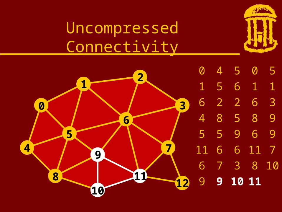
Uncompressed Connectivity
0
1
10
2
3
45
6
7
8
9
1112
0 4 5 0 5
1 5 6 1 1
6 2 2 6 3
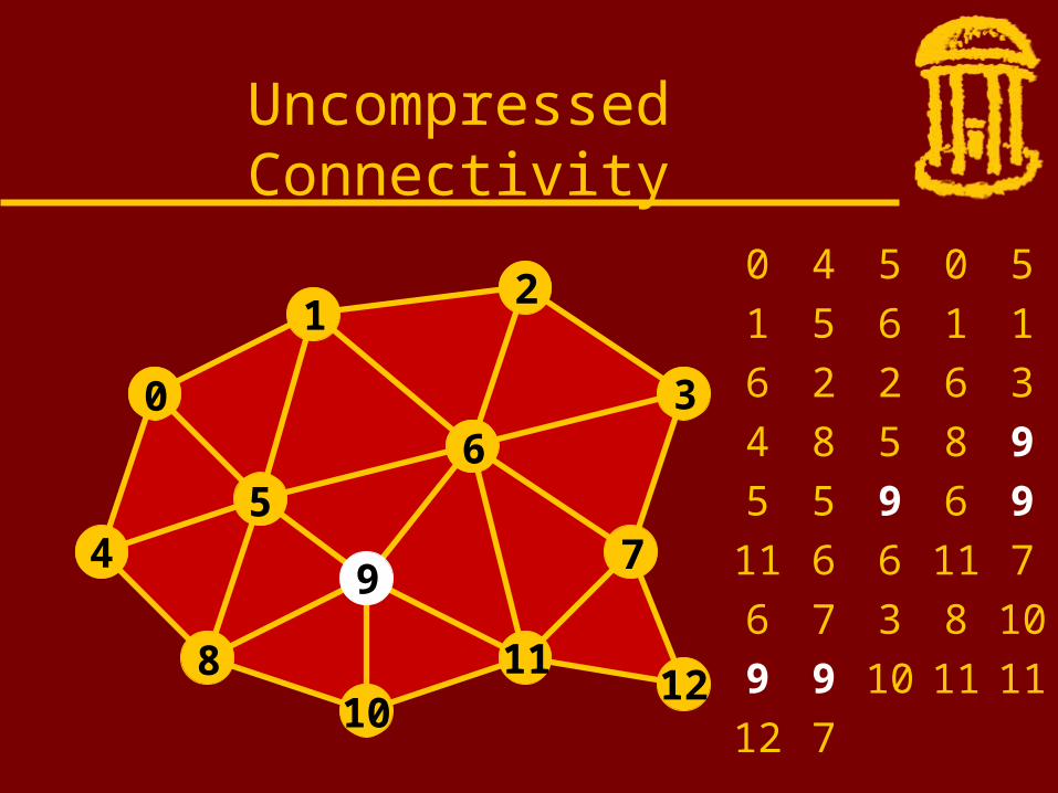
4 8 5 8 9
5 5 9 6 9
11 6 6 11 7
6 7 3 8 10
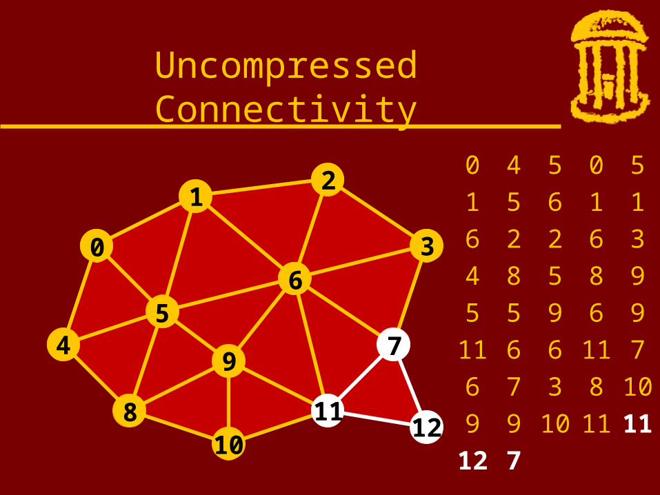
9 9 10 11 11
12 7
Uncompressed Connectivity

0
1
10
2
3
45
6
7
8
9
1112
0 4 5 0 5
1 5 6 1 1
6 2 2 6 3
4 8 5 8 9
5 5 9 6 9
11 6 6 11 7
6 7 3 8 10
9 9 10 11 11
12 7
Uncompressed Connectivity

0
1
10
2
3
45
6
7
8
9
1112
0 4 5 0 5
1 5 6 1 1
6 2 2 6 3
4 8 5 8 9
5 5 9 6 9
11 6 6 11 7
6 7 3 8 10
9 9 10 11 11
12 7
Uncompressed Connectivity
0
1
10
2
3
45
6
7
8
9
1112
0 4 5 0 5
1 5 6 1 1
6 2 2 6 3
4 8 5 8 9
5 5 9 6 9
11 6 6 11 7
6 7 3 8 10
9 9 10 11 11
12 7
Uncompressed Connectivity

0
1
10
2
3
45
6
7
8
9
1112
0 4 5 0 5
1 5 6 1 1
6 2 2 6 3
4 8 5 8 9
5 5 9 6 9
11 6 6 11 7
6 7 3 8 10
9 9 10 11 11
12 7
Uncompressed Connectivity

0
1
10
2
3
45
6
7
8
9
1112
0 4 5 0 5
1 5 6 1 1
6 2 2 6 3
4 8 5 8 9
5 5 9 6 9
11 6 6 11 7
6 7 3 8 10
9 9 10 11 11
12 7
Uncompressed Connectivity
6 log(n) bpv
Maximum Connectivity Compression for Triangle Meshes
Turan’s observation
• The fact that a planar graph can be decomposed into two spanning trees implies that it can be encoded in a constant number of bits.
• The fact that a planar graph can be decomposed into two spanning trees implies that it can be encoded in a constant number of bits.
• The two spanning trees are:– a vertex spanning tree– its dual triangle spanning tree
Turan’s observation
• The fact that a planar graph can be decomposed into two spanning trees implies that it can be encoded in a constant number of bits.
• The two spanning trees are:– a vertex spanning tree– its dual triangle spanning tree
• He gave an encoding that uses 12 bits per vertex (bpv).
Turan’s observation

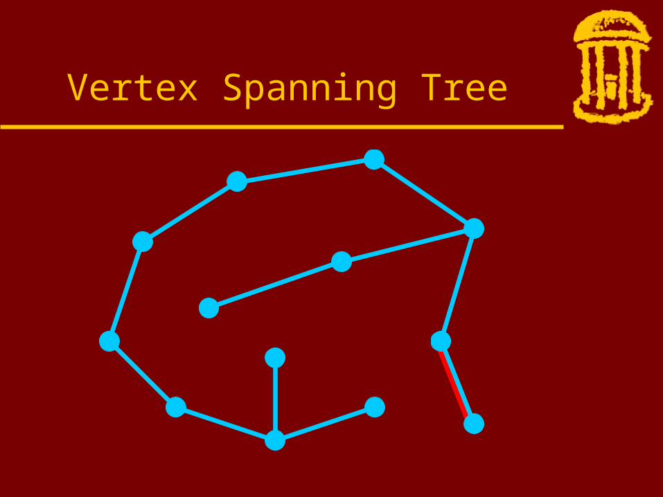
Vertex Spanning Tree

Vertex Spanning Tree
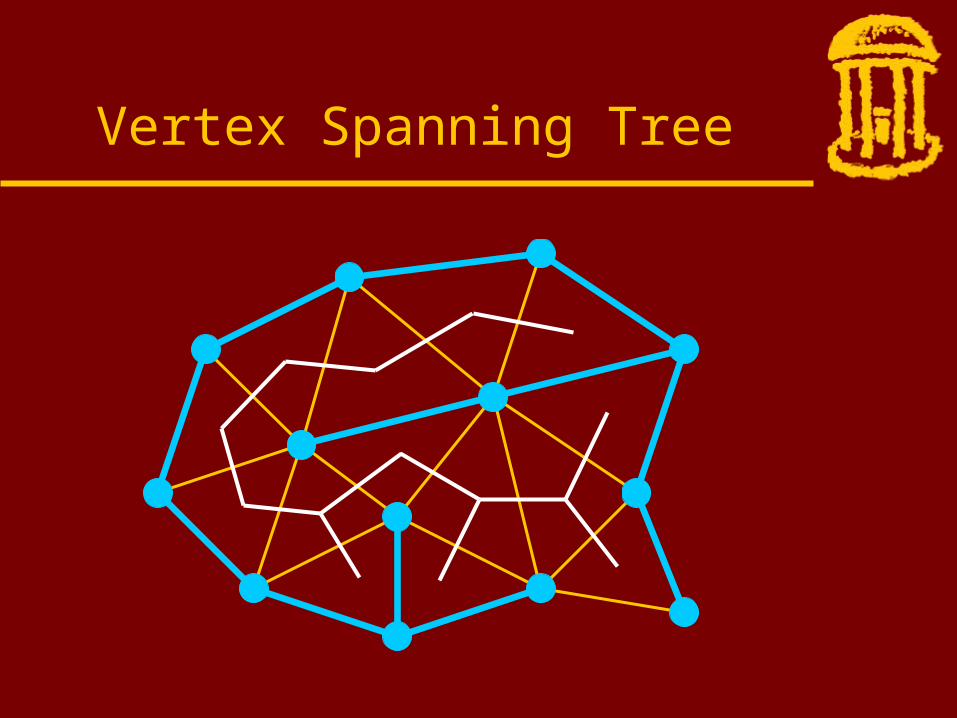
Vertex Spanning Tree

Triangle Spanning Tree
Vertex Spanning Tree

• Keeler Westbrook [95]
• Taubin Rossignac [96]
• Tauma Gotsman [98]
• Rossignac [98]
• DeFloriani et al [99]
• Isenburg Snoeyink [99]
Previous work

• Keeler Westbrook [95]
• Taubin Rossignac [96]
• Tauma Gotsman [98]
• Rossignac [98]
• DeFloriani et al [99]
• Isenburg Snoeyink [99]
Short Encodings of Planar Graphs and Maps
4.6 bpv (4.6)
Previous work

• Keeler Westbrook [95]
• Taubin Rossignac [96]
• Tauma Gotsman [98]
• Rossignac [98]
• DeFloriani et al [99]
• Isenburg Snoeyink [99]
Topological Surgery
2.4 ~ 7.0 bpv (--)
Previous work
• Keeler Westbrook [95]
• Taubin Rossignac [96]
• Tauma Gotsman [98]
• Rossignac [98]
• DeFloriani et al [99]
• Isenburg Snoeyink [99]
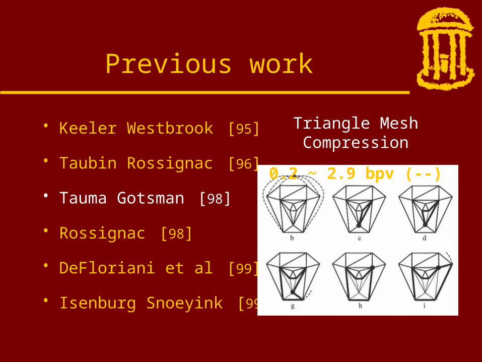
Triangle Mesh Compression
0.2 ~ 2.9 bpv (--)
Previous work

• Keeler Westbrook [95]
• Taubin Rossignac [96]
• Tauma Gotsman [98]
• Rossignac [98]
• DeFloriani et al [99]
• Isenburg Snoeyink [99]
Edgebreaker
3.2 ~ 4.0 bpv (4.0)
Previous work

• Keeler Westbrook [95]
• Taubin Rossignac [96]
• Tauma Gotsman [98]
• Rossignac [98]
• DeFloriani et al [99]
• Isenburg Snoeyink [99]
A Simple and EfficientEncoding for Triangle
Meshes4.2 ~ 5.4 bpv (6.0)
Previous work
• Keeler Westbrook [95]
• Taubin Rossignac [96]
• Tauma Gotsman [98]
• Rossignac [98]
• DeFloriani et al [99]
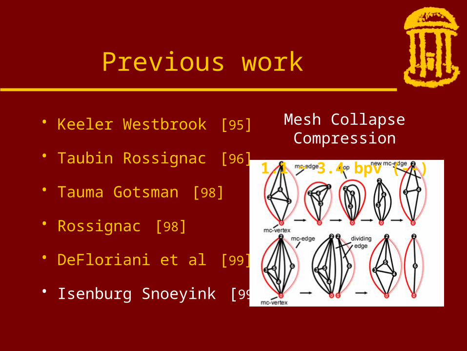
• Isenburg Snoeyink [99]
Mesh Collapse Compression
1.1 ~ 3.4 bpv (--)
Previous work
Triangle Fixer:
Edge-based Connectivity Compression
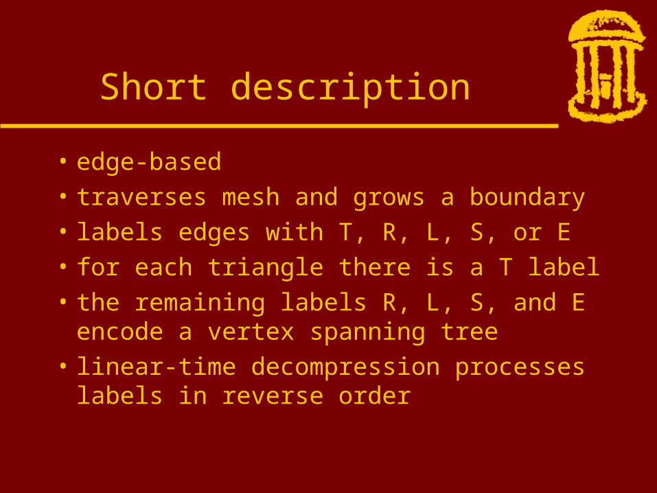
• edge-based• traverses mesh and grows a boundary• labels edges with T, R, L, S, or E• for each triangle there is a T label• the remaining labels R, L, S, and E
encode a vertex spanning tree• linear-time decompression processes
labels in reverse order
Short description

Encoding scheme
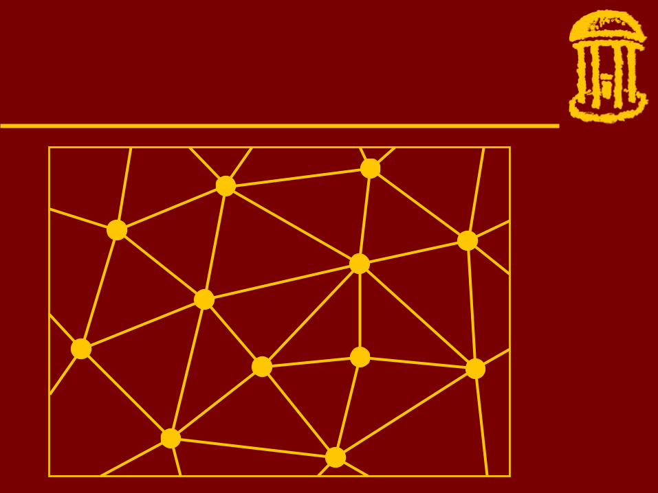
An initial active boundary is defined in cw order around an arbitrary edge of the
mesh.
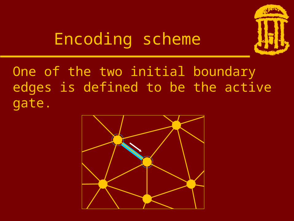
One of the two initial boundary edges is defined to be the active gate.
Encoding scheme
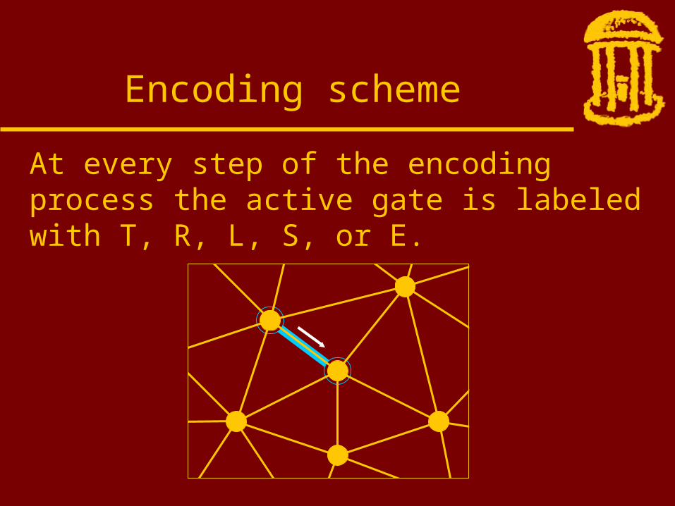
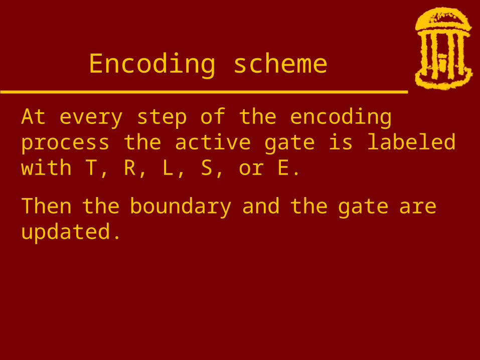
At every step of the encoding process the active gate is labeled with T, R, L, S, or E.
Encoding scheme
At every step of the encoding process the active gate is labeled with T, R, L, S, or E.
Then the boundary and the gate are
updated.
Encoding scheme
At every step of the encoding process the active gate is labeled with T, R, L, S, or E.
Then the boundary and the gate are
updated.
The boundary is expanded (T), is shrunk (R and L), is split (S), or is terminated (E).
Encoding scheme
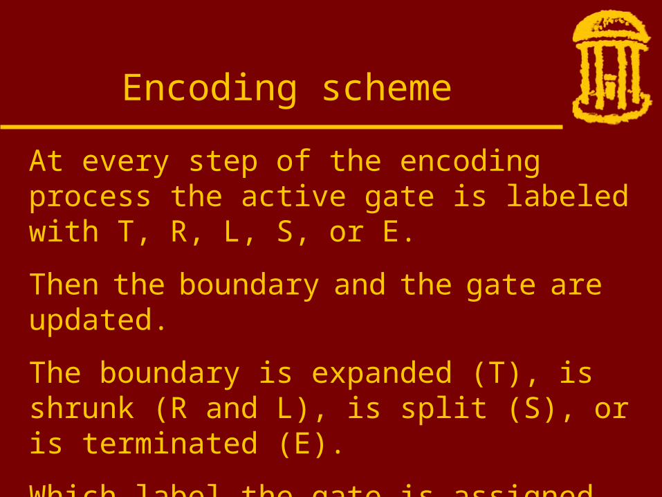
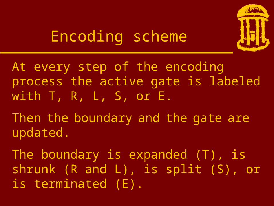
At every step of the encoding process the active gate is labeled with T, R, L, S, or E.
Then the boundary and the gate are
updated.
The boundary is expanded (T), is shrunk (R and L), is split (S), or is terminated (E).
Which label the gate is assigned depends on its adjacency relation with the boundary.
Encoding scheme

For each label T, R, L, S, and E we will now explain:
(1) for which active gate <-> boundary adjacency relation it applies
(2) how the boundary is updated
(3) how the active gate is updated
Encoding scheme
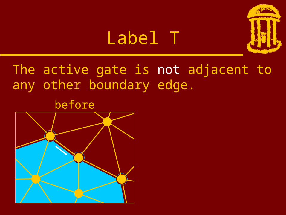
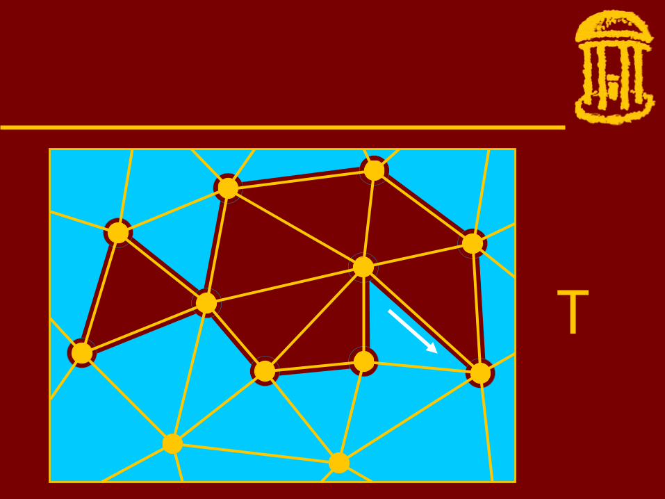
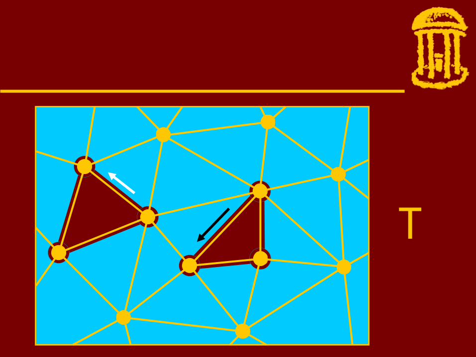
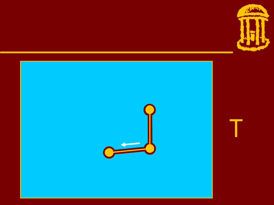
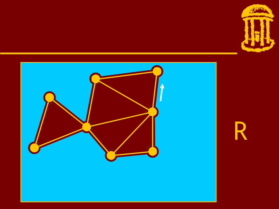
Label T
before
The active gate is not adjacent to any other boundary edge.
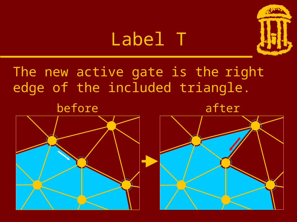
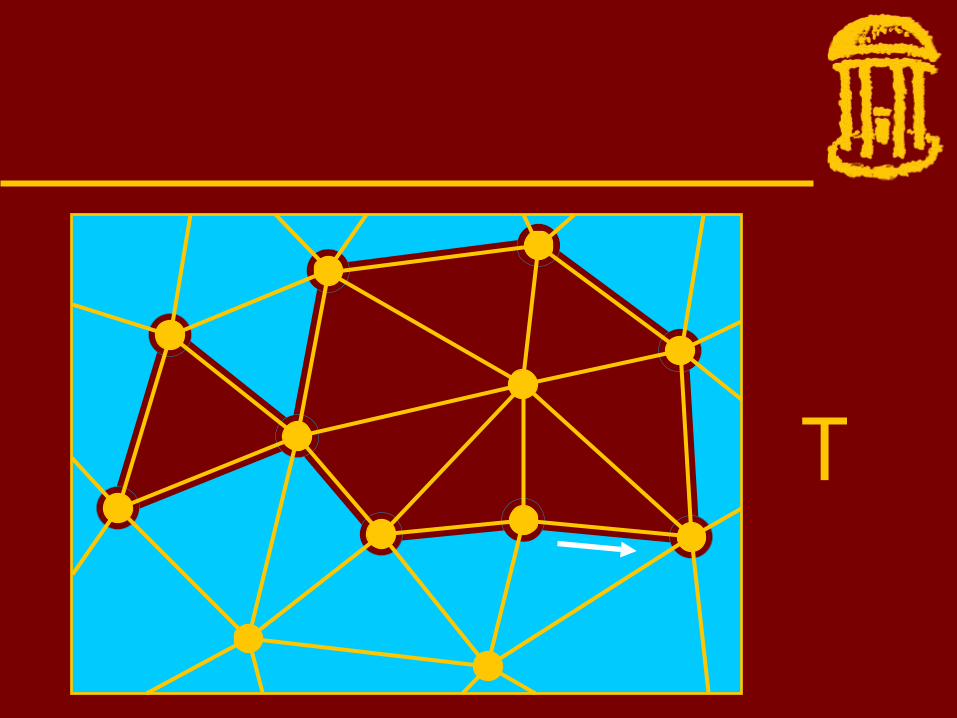
Label T
before after
The new active gate is the right edge of the included triangle.
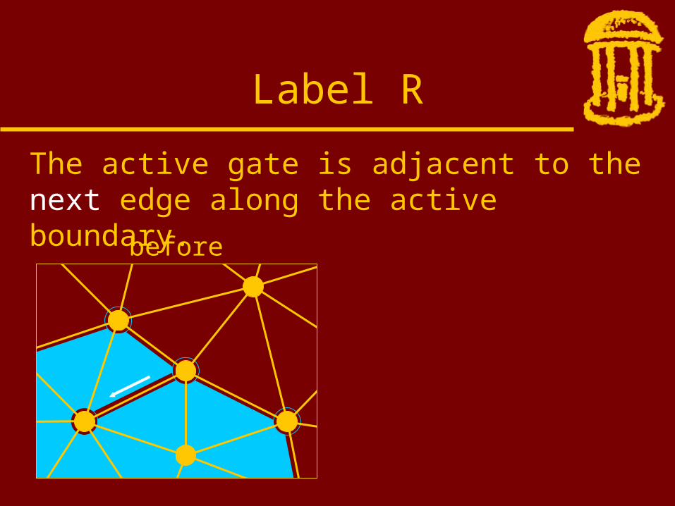
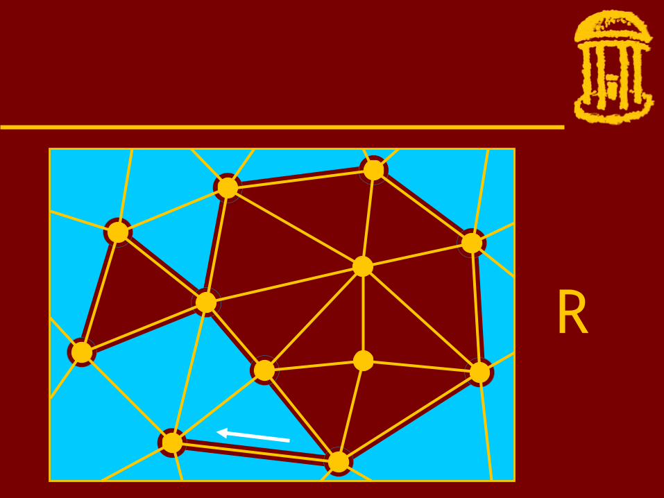
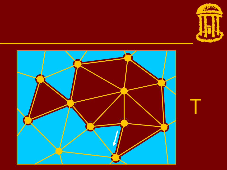
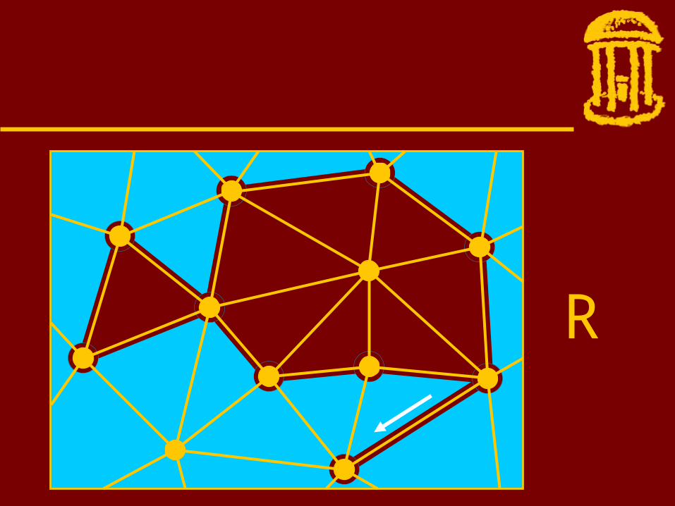
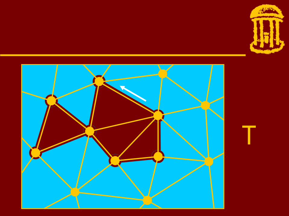
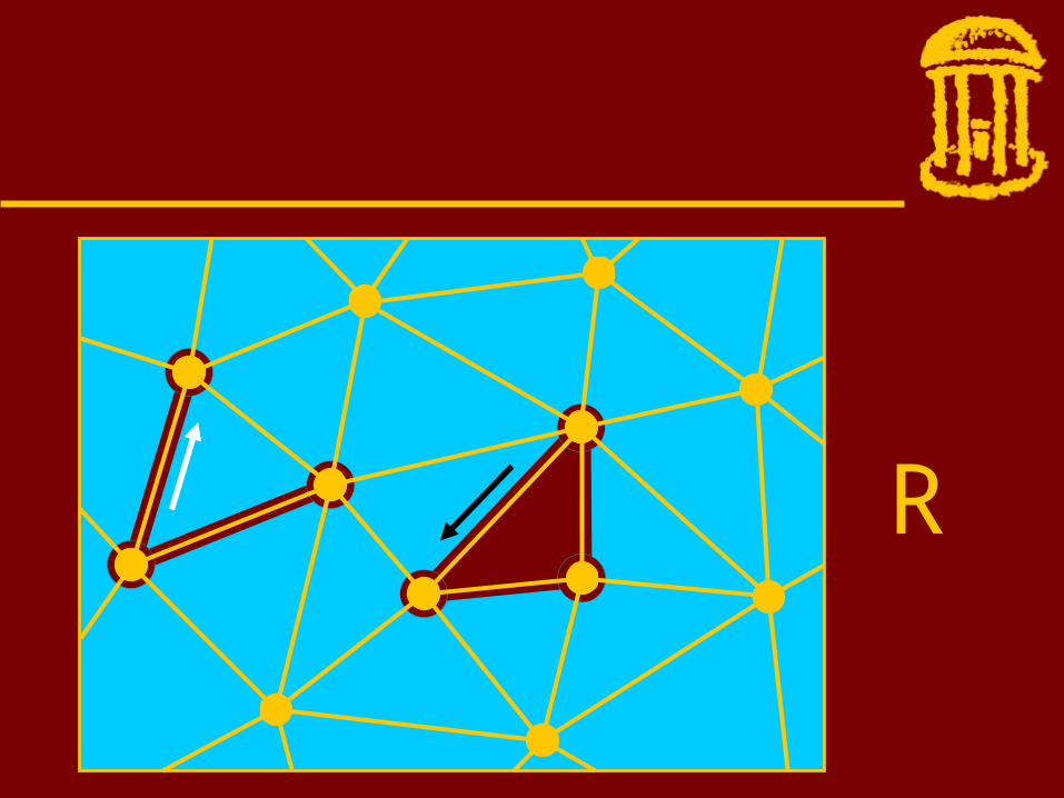
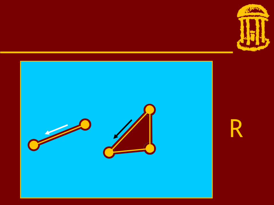
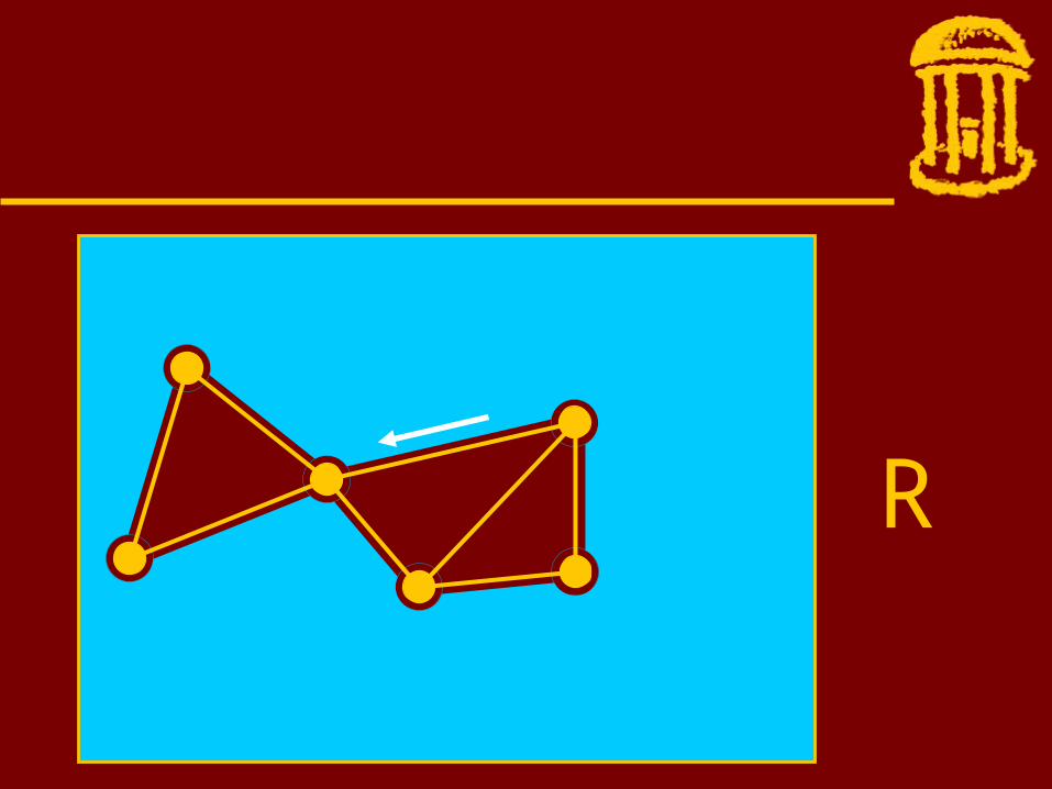
Label R
before
The active gate is adjacent to the next edge along the active boundary.
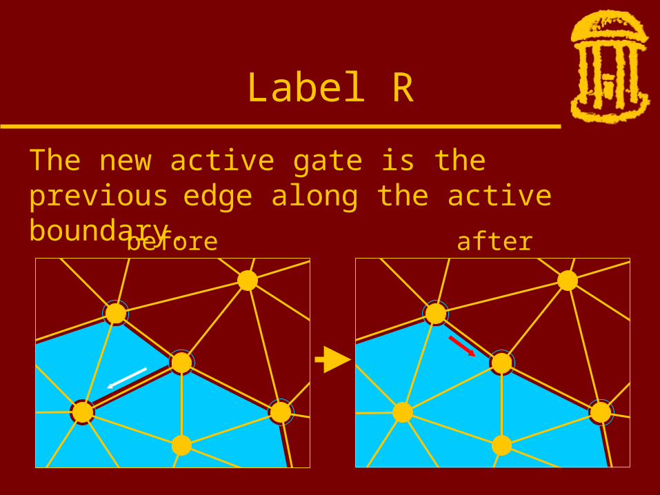
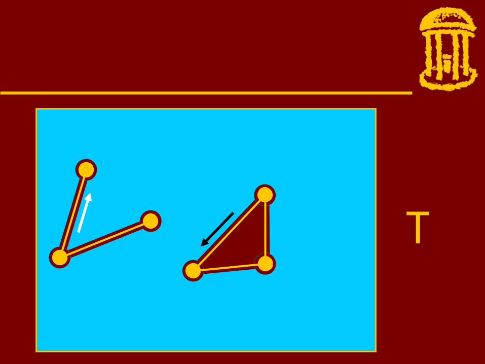
Label R
before after
The new active gate is the previous edge along the active boundary.
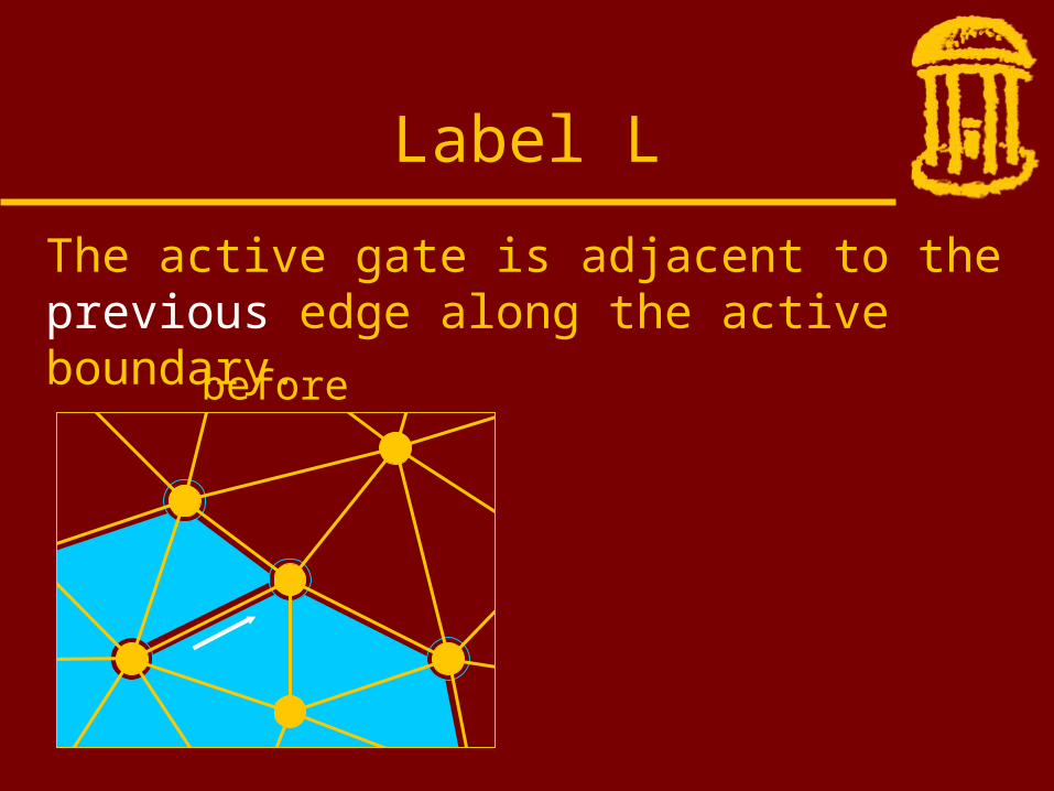
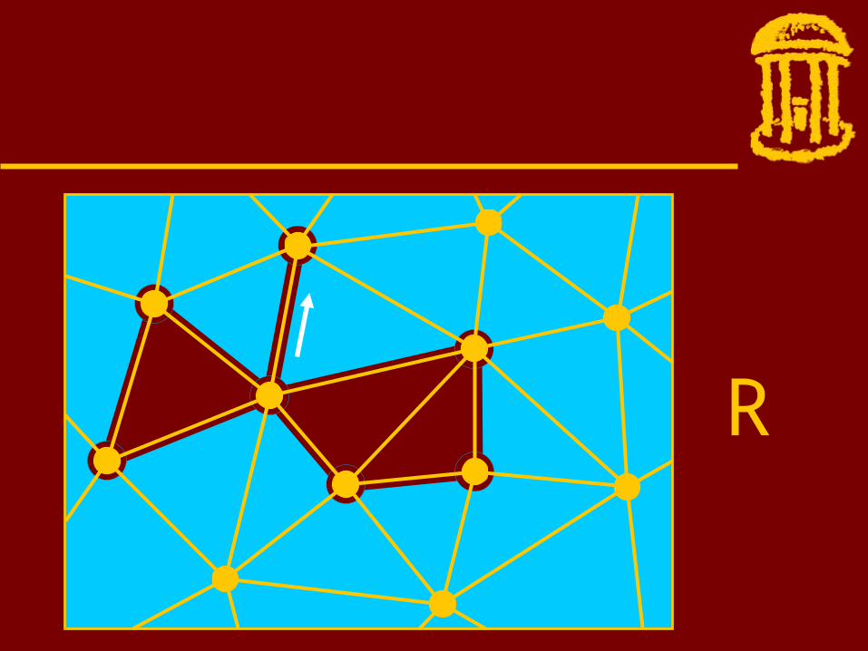
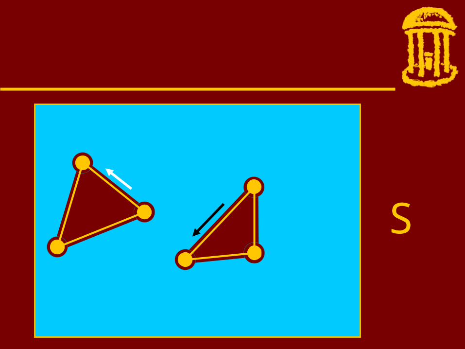
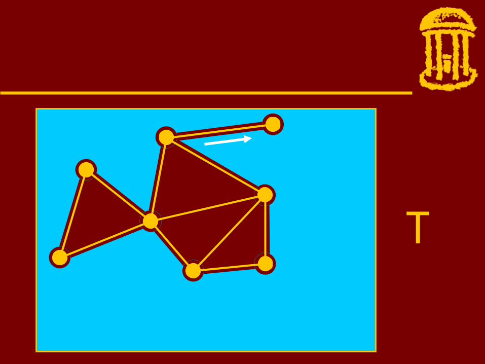
Label L
before
The active gate is adjacent to the previous edge along the active boundary.

Label L
before after
The new active gate is the next edge along the active boundary.
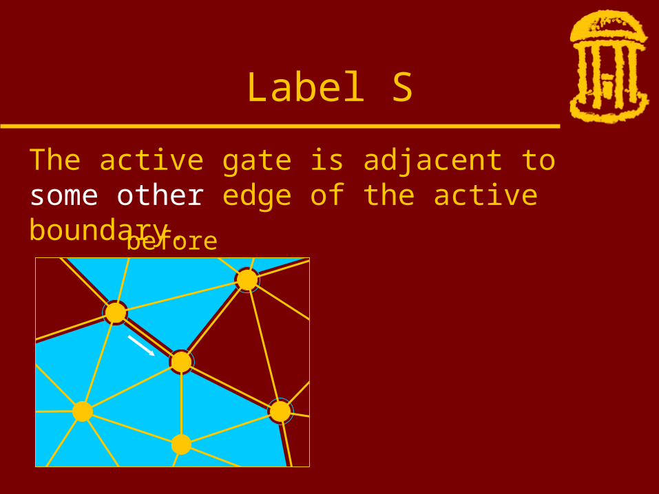
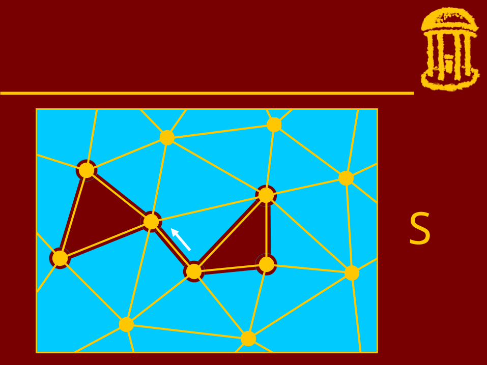
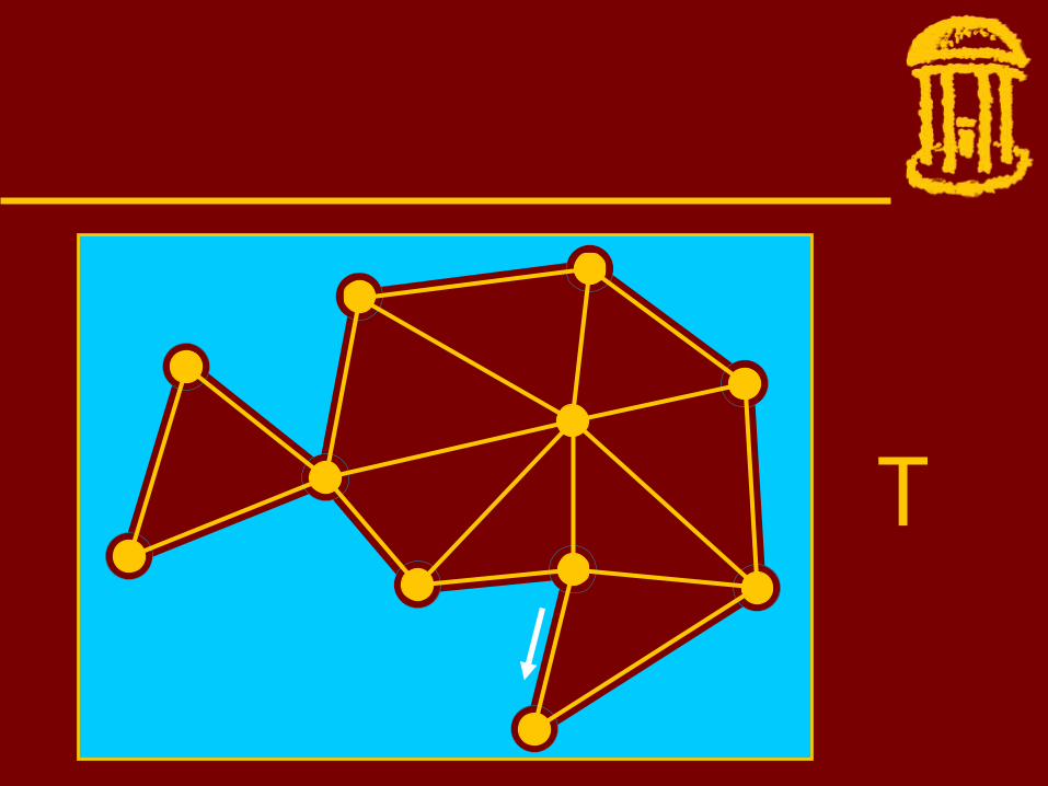
Label S
before
The active gate is adjacent to some other edge of the active boundary.

Label S
before after
The new active gate is the previous and the next edge along the active boundary.

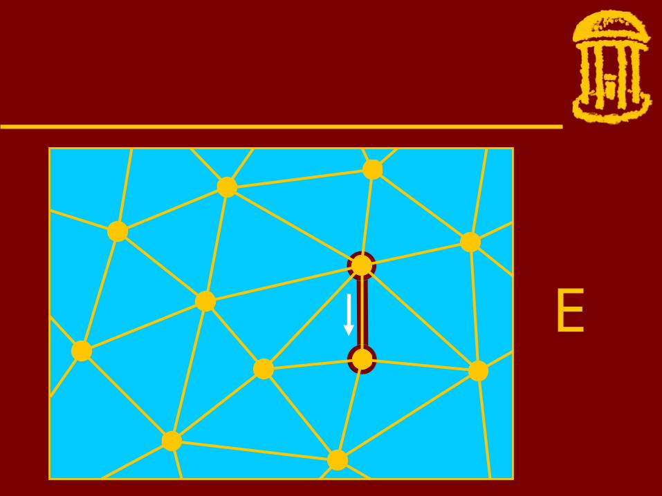
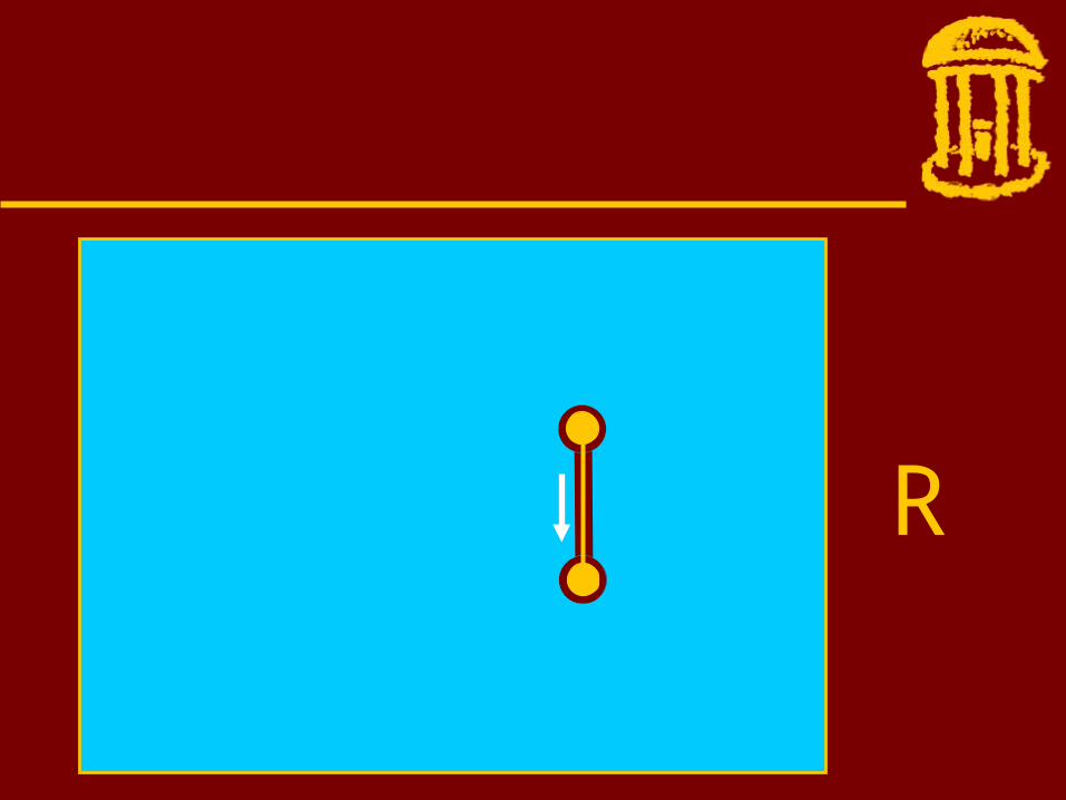
Label E
before
The active gate is adjacent to the previous and the next edge along the active boundary.

Label E
before after
The new active gate is popped from the stack. If the stack is empty we terminate.
Example Run - Encoding

T

T
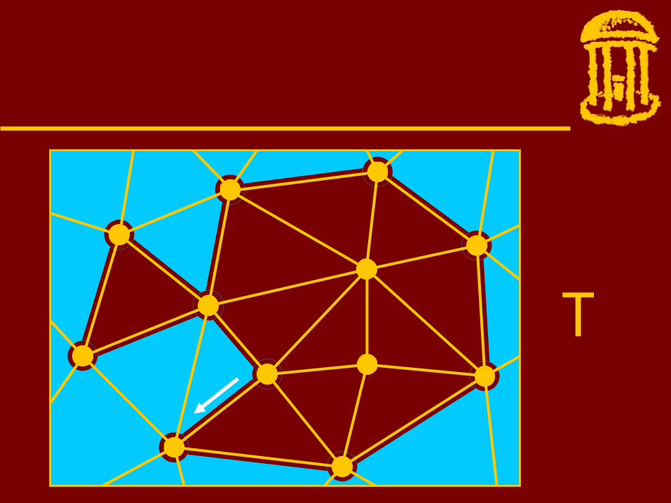
T
R

T
T
R
T
T

R

T

R

T

R
T
R

T
S
T
R

E

T

R
E


Example Run - Decoding

E
R
T

E
R
T
S

T
R

T

R
T
R

T

R

T

T

R

T
T

R

T

T

T


Holes and Handles

Encoding a hole
• use a new label H• associate an integer called size with
the label that specifies the number of edges/vertices around the hole
• there is one label Hsize per hole
• the total number of labels does not change, it is still equal to the number of edges in the mesh

Label Hsize
before
hole
The active gate is adjacent to a hole of size edges/vertices.
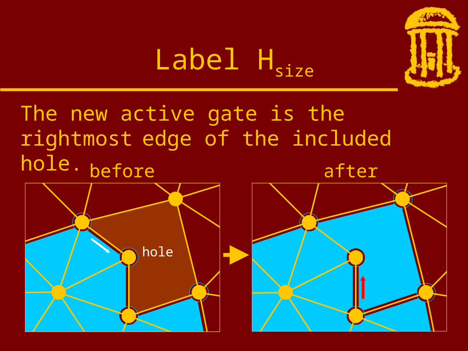
Label Hsize
before after
hole
The new active gate is the rightmost
edge of the included hole.
Encoding a handle
• use a new label M• associate three integers called index,
offset1, and offset2 with the label that
specify the current configuration
• there is one label Midx,off1,off2 per handle
• the total number of labels does not change, it is still equal to the number of edges in the mesh
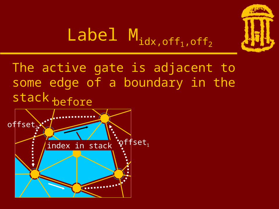
Label Midx,off1,off2
before
offset1
offset2
index in stack
The active gate is adjacent to some edge of a boundary in the stack.
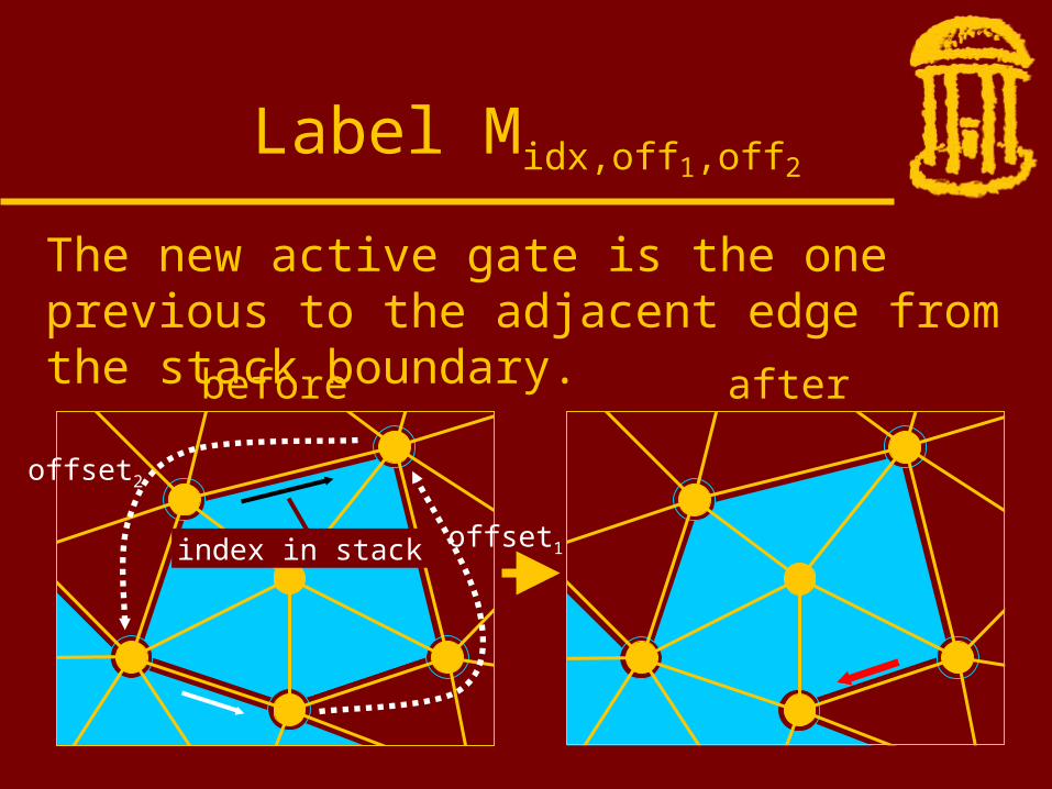
Label Midx,off1,off2
before after
offset1
The new active gate is the one previous to the adjacent edge from the stack boundary.
offset2
index in stack
Compressing the label sequence

label encoding
• The number of labels T, R, L, S, and E equals the number of edges in the mesh. A simple mesh with v vertices has 3v - 6 edges and 2v - 4 triangles.
• This means that 2v - 4 labels are of type T and the remaining v - 2 labels are of type R, L, S, and E.
• A 13333 label encoding guarantees to use exactly 5v - 10 bits.

label bits code
T 1 0R 3 100L 3 101S 3 110E 3 111
guarantees 5 bits per vertex
13333 label encoding
label bits code
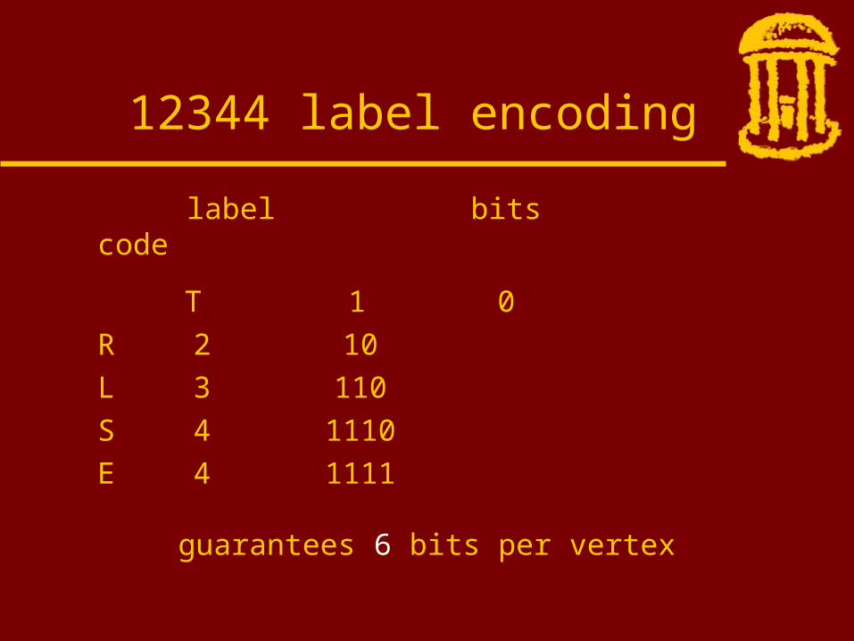
T 1 0R 2 10L 3 110S 4 1110E 4 1111
guarantees 6 bits per vertex
12344 label encoding

previous label current encoding
T 1 2 4 3 4R 1 2 4 3 4L 1 4 2 4 3S 1 4 2 4 3E 1 2 4 4 3
guarantees 6 bits per vertex
fixed bit encoding
• approaches the entropy of the label sequence
• adaptive version • three label memory• due to small number of different
symbols, probability tables require less than 8KB
• implemented with fast bit operations
arithmetic encoding

Example results
vertices fixedmesh
33204 4.05phone
34834 4.00bunny
10952 4.22skull
766 4.09eight
3897 4.16femur
3078 3.99cow
aac-3
2.70
1.73
2.96
1.43
3.05
2.36
2562 4.00shape
6475 4.01fandisk
0.77
1.67
holes
3
5
--
--
--
22
--
--
handles
--
--
51
2
2
--
--
--

Sneak Preview

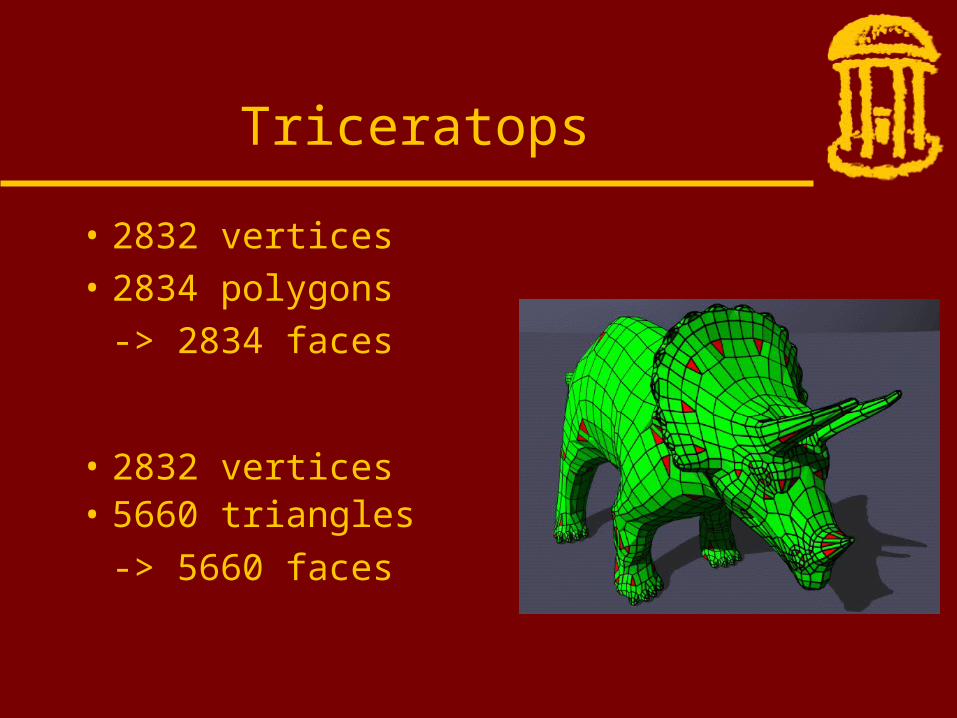
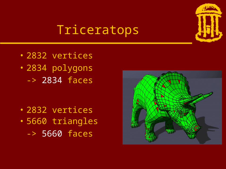
Triceratops
• 2832 vertices
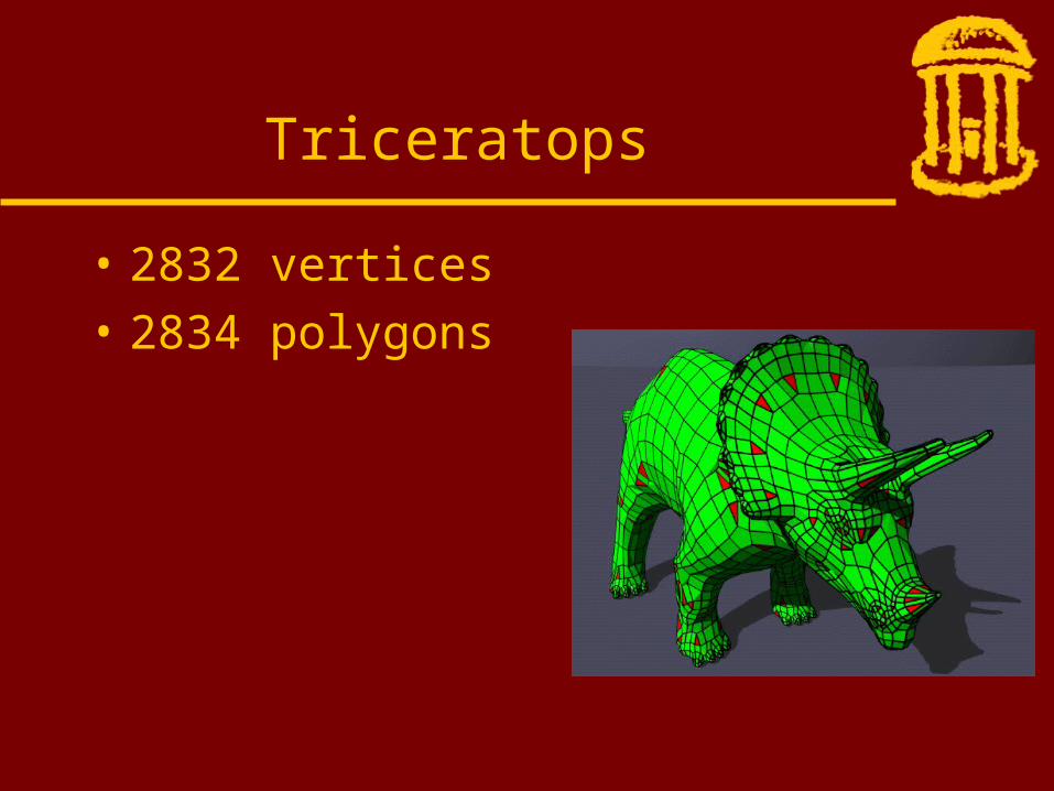
• 2832 vertices• 2834 polygons
Triceratops

• 2832 vertices• 2834 polygons
– 346 triangles
Triceratops

• 2832 vertices• 2834 polygons
– 346 triangles– 2266 quadrilaterals
Triceratops

• 2832 vertices• 2834 polygons
– 346 triangles– 2266 quadrilaterals– 140 pentagons
Triceratops
• 2832 vertices• 2834 polygons
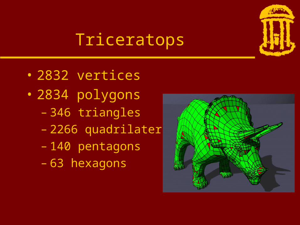
– 346 triangles– 2266 quadrilaterals– 140 pentagons– 63 hexagons
Triceratops

• 2832 vertices• 2834 polygons
– 346 triangles– 2266 quadrilaterals– 140 pentagons– 63 hexagons– 10 heptagons
Triceratops

• 2832 vertices• 2834 polygons
– 346 triangles– 2266 quadrilaterals– 140 pentagons– 63 hexagons– 10 heptagons – 7 octagons
Triceratops
• 2832 vertices• 2834 polygons
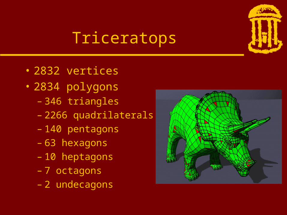
– 346 triangles– 2266 quadrilaterals– 140 pentagons– 63 hexagons– 10 heptagons – 7 octagons– 2 undecagons
Triceratops

• 2832 vertices• 2834 polygons
Triceratops
• 2832 vertices• 2834 polygons
-> 11328 corners
Triceratops
• 2832 vertices• 2834 polygons
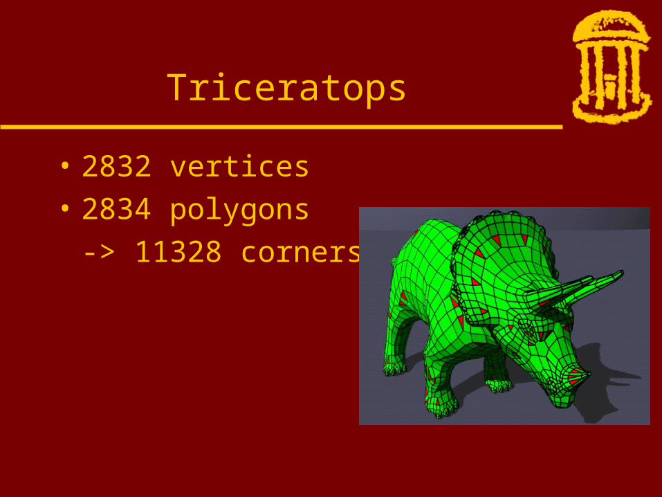
-> 11328 corners
• 2832 vertices• 5660 triangles
Triceratops

• 2832 vertices• 2834 polygons
-> 11328 corners
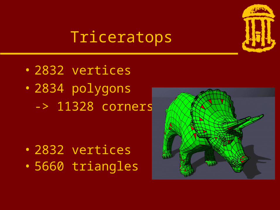
• 2832 vertices• 5660 triangles
-> 16980 corners
Triceratops

• 2832 vertices• 2834 polygons
-> 11328 corners
• 2832 vertices• 5660 triangles
-> 16980 corners
Triceratops

• 2832 vertices• 2834 polygons
Triceratops

• 2832 vertices• 2834 polygons
-> 2834 faces
Triceratops

• 2832 vertices• 2834 polygons
-> 2834 faces
• 2832 vertices• 5660 triangles
Triceratops
• 2832 vertices• 2834 polygons
-> 2834 faces
• 2832 vertices• 5660 triangles
-> 5660 faces
Triceratops
• 2832 vertices• 2834 polygons
-> 2834 faces
• 2832 vertices• 5660 triangles
-> 5660 faces
Triceratops

Beethoven
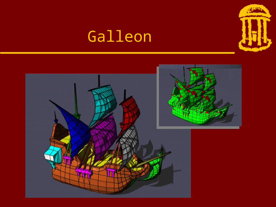
Galleon
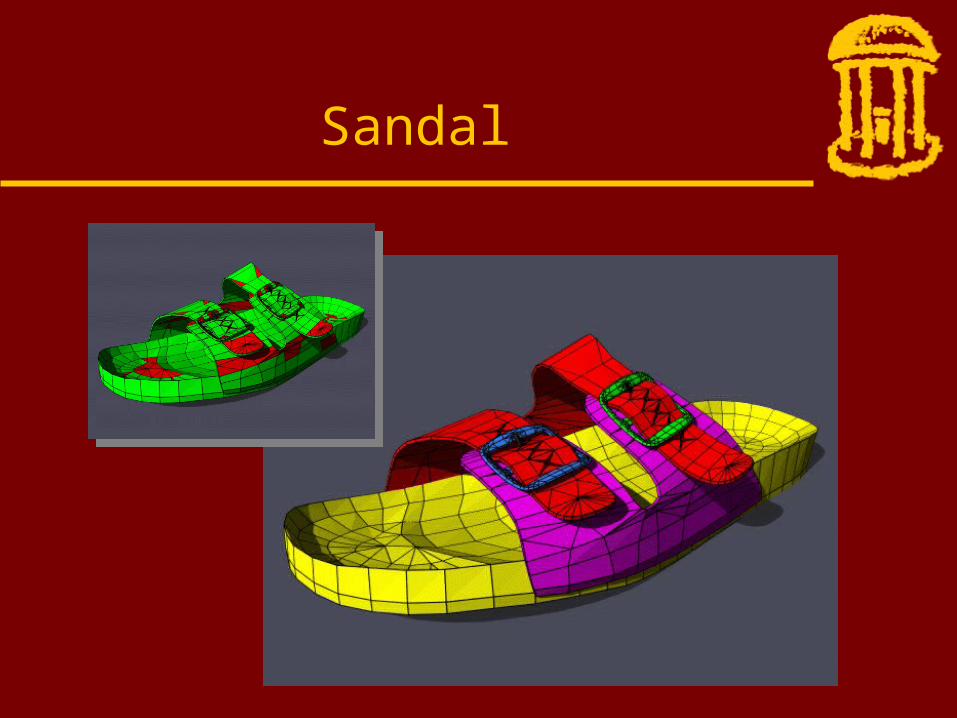
Sandal
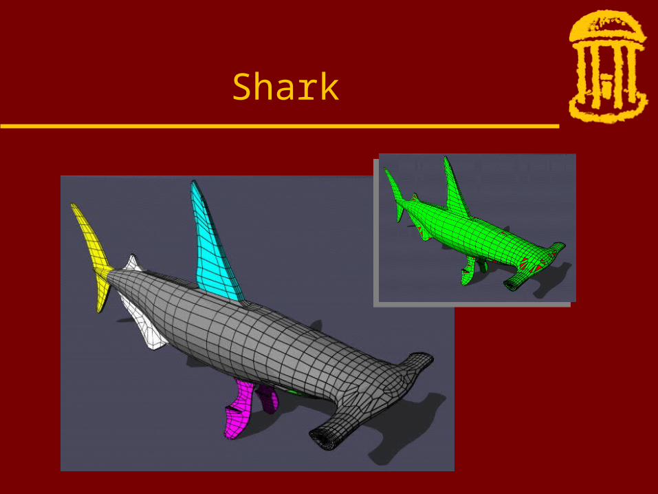
Shark

Cessna
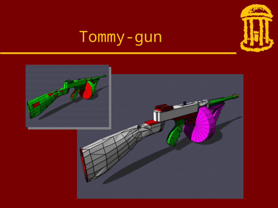
Tommy-gun

Short Example Run
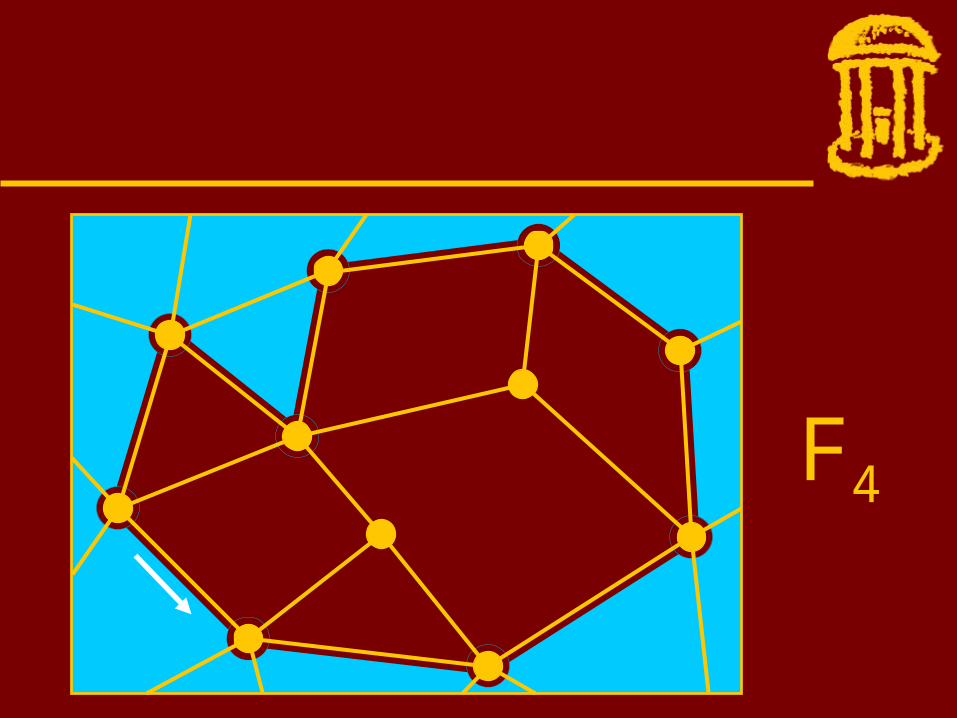
F4

F3
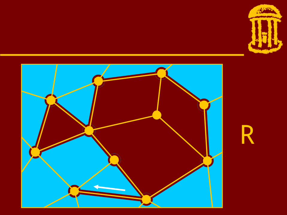
R

F5

R

F4
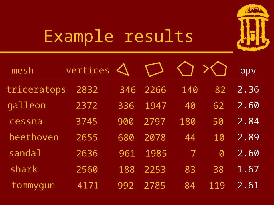
Example results
vertices bpvmesh
2832 2.36triceratops
2372 2.60galleon
3745 2.84cessna
2655 2.89beethoven
2636 2.60sandal
2560 1.67shark
4171tommygun 2.61
346
336
900
680
961
188
992
2266
1947
2797
2078
1985
2253
2785
140
40
180
44
7
83
84
82
62
50
10
0
38
119

Face Fixer:Compressing Polygon Meshes
with Properties
SIGGRAPH ’2000
http://www.cs.unc.edu/~isenburg/papers/is-ff-00.pdf

Current Work
• Patch Fixer– Find frequent patches in mesh and use
their repeating structure for encoding.
• Tetra Fixer– Compressing Tetrahedral Meshes
• Volume Fixer– Compressing Volume Data composed of
Tetrahedrons and Octahedrons with support for cell group structures.

Acknowledgements
• Paola Magillo for providing her set of example meshes
• Michael Maniscalco and Frederick Wheeler for technical insights on arithmetic coding
• Jarek Rossignac and Davis King for fruitful discussions
• my supervisor Jack Snoeyink for reviewing the paper


