113
Uniform Algebras Over Complete Valued Fields Jonathan W. Mason, MMath. Thesis submitted to The University of Nottingham for the degree of Doctor of Philosophy March 2012

Uniform Algebras Over Complete
Valued Fields
Jonathan W. Mason, MMath.
Thesis submitted to The University of Nottingham
for the degree of Doctor of Philosophy
March 2012

For OlesyaFollow the Romany patteran
West to the sinking sun,Till the junk-sails lift through the houseless drift.
And the east and west are one.1
1From Rudyard Kipling’s poem The Gipsy Trail.
i

Abstract
UNIFORM algebras have been extensively investigated because of their importance in
the theory of uniform approximation and as examples of complex Banach algebras. An
interesting question is whether analogous algebras exist when a complete valued field
other than the complex numbers is used as the underlying field of the algebra. In the
Archimedean setting, this generalisation is given by the theory of real function alge-
bras introduced by S. H. Kulkarni and B. V. Limaye in the 1980s. This thesis establishes
a broader theory accommodating any complete valued field as the underlying field by
involving Galois automorphisms and using non-Archimedean analysis. The approach
taken keeps close to the original definitions from the Archimedean setting.
Basic function algebras are defined and generalise real function algebras to all complete
valued fields whilst retaining the obligatory properties of uniform algebras.
Several examples are provided. A basic function algebra is constructed in the non-
Archimedean setting on a p-adic ball such that the only globally analytic elements of
the algebra are constants.
Each basic function algebra is shown to have a lattice of basic extensions related to the
field structure. In the non-Archimedean setting it is shown that certain basic function
algebras have residue algebras that are also basic function algebras.
A representation theorem is established. Commutative unital Banach F-algebras with
square preserving norm and finite basic dimension are shown to be isometrically F-
isomorphic to some subalgebra of a Basic function algebra. The condition of finite
basic dimension is always satisfied in the Archimedean setting by the Gel’fand-Mazur
Theorem. The spectrum of an element is considered.
The theory of non-commutative real function algebras was established by K. Jarosz in
2008. The possibility of their generalisation to the non-Archimedean setting is estab-
lished in this thesis and also appeared in a paper by J. W. Mason in 2011.
In the context of complex uniform algebras, a new proof is given using transfinite
induction of the Feinstein-Heath Swiss cheese “Classicalisation” theorem. This new
proof also appeared in a paper by J. W. Mason in 2010.
ii
Acknowledgements
I would particular like to thank my supervisor J. F. Feinstein for his guidance and en-
thusiasm over the last four years. Through his expert knowledge of Banach algebra
theory he has helped me to identify several productive lines of research whilst always
allowing me the freedom required to make the work my own.
In addition to my supervisor, I. B. Fesenko also positively influenced the direction of
my research. During my doctoral training I undertook a postgraduate training module
on the theory of local fields given by I. B. Fesenko. With extra reading, this enabled
me to work both in the Archimedean and non-Archimedean settings as implicitly sug-
gested by my thesis title.
It was a pleasure to know my friends in the algebra and analysis group at Nottingham
and I thank them for their interest in my work and hospitality.
I am grateful to the School of Mathematical sciences at the University of Nottingham
for providing funds in support of my conference participation and visits.
Similarly I appreciate the support given to me by the EPSRC through a Doctoral Train-
ing Grant.
This PhD thesis was examined by A. G. O’Farrell and J. Zacharias who I thank for their
time and interest in my work.
iii
Contents
1 Introduction 1
1.1 Background and Overview . . . . . . . . . . . . . . . . . . . . . . . . . . 1
1.2 Summary . . . . . . . . . . . . . . . . . . . . . . . . . . . . . . . . . . . . . 3
2 Complete valued fields 5
2.1 Introduction . . . . . . . . . . . . . . . . . . . . . . . . . . . . . . . . . . . 5
2.1.1 Series expansions of elements of valued fields . . . . . . . . . . . 7
2.1.2 Examples of complete valued fields . . . . . . . . . . . . . . . . . 9
2.1.3 Topological properties of complete valued fields . . . . . . . . . . 12
2.2 Extending complete valued fields . . . . . . . . . . . . . . . . . . . . . . . 14
2.2.1 Extensions . . . . . . . . . . . . . . . . . . . . . . . . . . . . . . . . 15
2.2.2 Galois theory . . . . . . . . . . . . . . . . . . . . . . . . . . . . . . 20
3 Functions and algebras 22
3.1 Functional analysis over complete valued fields . . . . . . . . . . . . . . 22
3.1.1 Analytic functions . . . . . . . . . . . . . . . . . . . . . . . . . . . 24
3.2 Banach F-algebras . . . . . . . . . . . . . . . . . . . . . . . . . . . . . . . . 28
3.2.1 Spectrum of an element . . . . . . . . . . . . . . . . . . . . . . . . 29
4 Uniform algebras 34
4.1 Complex uniform algebras . . . . . . . . . . . . . . . . . . . . . . . . . . . 34
4.1.1 Swiss cheese sets in the complex plane . . . . . . . . . . . . . . . 36
4.1.2 Classicalisation theorem . . . . . . . . . . . . . . . . . . . . . . . . 39
4.2 Non-complex analogs of uniform algebras . . . . . . . . . . . . . . . . . . 48
iv
CONTENTS
4.2.1 Real function algebras . . . . . . . . . . . . . . . . . . . . . . . . . 50
5 Commutative generalisation over complete valued fields 53
5.1 Main definitions . . . . . . . . . . . . . . . . . . . . . . . . . . . . . . . . . 53
5.2 Generalisation theorems . . . . . . . . . . . . . . . . . . . . . . . . . . . . 55
5.3 Examples . . . . . . . . . . . . . . . . . . . . . . . . . . . . . . . . . . . . . 59
5.4 Non-Archimedean new basic function algebras from old . . . . . . . . . 65
5.4.1 Basic extensions . . . . . . . . . . . . . . . . . . . . . . . . . . . . . 65
5.4.2 Residue algebras . . . . . . . . . . . . . . . . . . . . . . . . . . . . 67
6 Representation theory 79
6.1 Further Banach rings and Banach F-algebras . . . . . . . . . . . . . . . . 79
6.2 Representations . . . . . . . . . . . . . . . . . . . . . . . . . . . . . . . . . 88
6.2.1 Established theorems . . . . . . . . . . . . . . . . . . . . . . . . . . 88
6.2.2 Motivation . . . . . . . . . . . . . . . . . . . . . . . . . . . . . . . . 90
6.2.3 Representation under finite basic dimension . . . . . . . . . . . . 91
7 Non-commutative generalisation and open questions 98
7.1 Non-commutative generalisation . . . . . . . . . . . . . . . . . . . . . . . 98
7.1.1 Non-commutative real function algebras . . . . . . . . . . . . . . 98
7.1.2 Non-commutative non-Archimedean analogs . . . . . . . . . . . 100
7.2 Open questions . . . . . . . . . . . . . . . . . . . . . . . . . . . . . . . . . 101
References 105
v
CHAPTER 1
Introduction
This short chapter provides an informal overview of the material in this thesis. Justifi-
cation of the statements made in this chapter can therefore be found in the main body
of the thesis which starts at Chapter 2.
1.1 Background and Overview
Complex uniform algebras have been extensively investigated because of their impor-
tance in the theory of uniform approximation and as examples of complex Banach alge-
bras. Let CC(X) denote the complex Banach algebra of all continuous complex-valued
functions defined on a compact Hausdorff space X. A complex uniform algebra A is a
subalgebra of CC(X) that is complete with respect to the sup norm, contains the con-
stant functions making it a unital complex Banach algebra and separates the points of X
in the sense that for all x1, x2 ∈ X with x1 6= x2 there is f ∈ A satisfying f (x1) 6= f (x2).
Attempting to generalise this definition to other complete valued fields simply by re-
placing C with some other complete valued field L produces very limited results. This
is because the various versions of the Stone-Weierstrass theorem restricts our attention
to CL(X) in this case.
However the theory of real function algebras introduced by S. H. Kulkarni and B. V.
Limaye in the 1980s does provide an interesting generalisation of complex uniform
algebras. One important departure in the definition of these algebras from that of com-
plex uniform algebras is that they are real Banach algebras of continuous complex-
valued functions. Similarly the elements of the algebras introduced in this thesis are
also continuous functions that take values in some complete valued field or division
ring extending the field of scalars over which the algebra is a vector space.
A prominent aspect of the emerging theory is that it has a lot to do with representation.
As a very simple example the field of complex numbers itself is isometrically isomor-
phic to a real function algebra, all be it on a two point space.
1
CHAPTER 1: INTRODUCTION
When considering the generalisation of complex uniform algebras over all complete
valued fields I naturally wanted the complex uniform algebras and real function alge-
bras to appear directly as instances of the new theory. This resulted in the definition
of basic function algebras involving the use of a Galois automorphism and homeomor-
phic endofunction that interact in a useful way, see Definition 5.1.2. In retrospect these
particular algebras should more appropriately be referred to as cyclic basic function
algebras since the functions involved take values in some cyclic extension of the un-
derlying field of scalars of the algebra.
Necessarily this thesis starts by surveying complete valued fields and their properties.
The transition from the Archimedean setting to the non-Archimedean setting preserves
in places several of the nice properties that complete Archimedean fields have. How-
ever all complete non-Archimedean fields are totally disconnected, some of them are
not locally compact and there is no non-Archimedean analog of the Gel’fand-Mazur
Theorem.
On the other hand some complete non-Archimedean fields have interesting properties
that only appear in the non-Archimedean setting. Consider for example the closed unit
disc of the complex plane. It is closed under multiplication but not with respect to ad-
dition. In the non-Archimedean setting the closed unit ball OF, of a complete valued
field F, is a ring since in this case the valuation involved observes the strong version of
the triangle inequality, see Definition 2.1.1. The setMF = {a ∈ F : |a|F < 1} is a max-
imal ideal of OF from which the residue field F = OF/MF is obtained. The residue
field is of great importance in the study of such fields.
Similarly in the non-Archimedean setting we will see that certain basic function al-
gebras have residue algebras that are also basic function algebras. In the process of
proving this result an interesting fact is shown concerning a large class of complete
non-Archimedean fields. For such a field F and every finite extension L of F, extending
F as a valued field, it is shown that for each Galois automorphism g ∈ Gal(L/F) there
exists a set RL,g ⊆ OL of residue class representatives such that the restriction of g to
RL,g is an endofunction, i.e. a self map, onRL,g. This fact is probably known to certain
number theorists.
This thesis also includes several examples of basic function algebras and these are con-
sidered at depth. A new proof of an existing theorem in the setting of complex uniform
algebras is given and theory in the non-commutative setting is also considered.
With respect to commutative Banach algebra theory, Chapter 6 presents an interest-
ing new Gel’fand representation result extending those of the Archimedean setting. In
particular we have the following theorem where the condition of finite basic dimen-
sion is automatically satisfied in the Archimedean setting and compensates for the lack
of a Gel’fand-Mazur Theorem in the non-Archimedean setting. See Chapter 6 for full
2

CHAPTER 1: INTRODUCTION
details.
Theorem 1.1.1. Let F be a locally compact complete valued field with nontrivial valuation. Let
A be a commutative unital Banach F-algebra with ‖a2‖A = ‖a‖2A for all a ∈ A and finite basic
dimension. Then:
(i) if F is the field of complex numbers then A is isometrically F-isomorphic to a complex
uniform algebra on some compact Hausdorff space X;
(ii) if F is the field of real numbers then A is isometrically F-isomorphic to a real function
algebra on some compact Hausdorff space X;
(iii) if F is non-Archimedean then A is isometrically F-isomorphic to a non-Archimedean
analog of the real function algebras on some Stone space X where by a Stone space we
mean a totally disconnected compact Hausdorff space.
In particular A is isometrically F-isomorphic to some subalgebra A of a basic function algebra
and A separates the points of X.
Note that (i) and (ii) of Theorem 1.1.1 are the well known results from the Archimedean
setting. This brings us to the following summary.
1.2 Summary
Chapter 2: The relevant background concerning complete valued fields is provided. Several
examples are given and the topological properties of complete valued fields are
compared and discussed. A particularly useful and well known way of express-
ing the extension of a valuation is considered and the relevant Galois theory is
introduced.
Chapter 3: Some background concerning functional analysis over complete valued fields is
given. Analytic functions are discussed. Banach F-algebras are introduced and
the spectrum of an element is considered.
Chapter 4: Complex uniform algebras are introduced. In the context of complex uniform
algebras, a new proof is given using transfinite induction of the Feinstein-Heath
Swiss cheese “Classicalisation” theorem. This new proof also appeared in a paper
by J. W. Mason in 2010. This is followed by a preliminary discussion concerning
non-complex analogs of uniform algebras. Real function algebras are introduced.
Chapter 5: Basic function algebras are defined providing the required generalisation of real
function algebras to all complete valued fields. A generalisation theorem proves
3

CHAPTER 1: INTRODUCTION
that Basic function algebras have the obligatory properties of uniform algebras.
Several examples are provided. Complex uniform algebras and real function al-
gebras now appear as instances of the new theory. A basic function algebra is
constructed in the non-Archimedean setting on a p-adic ball such that the only
globally analytic elements of the algebra are constants.
Each basic function algebra is shown to have a lattice of basic extensions related
to the field structure. Further, in the non-Archimedean setting it is shown that
certain basic function algebras have residue algebras that are also basic function
algebras. To prove this each Galois automorphism, for certain field extensions, is
shown to restrict to an endofunction on some set of residue class representatives.
Chapter 6: A representation theorem is established in the context of locally compact com-
plete fields with nontrivial valuation. For such a field F, commutative unital
Banach F-algebras with square preserving norm and finite basic dimension are
shown to be isometrically F-isomorphic to some subalgebra of a Basic function
algebra. The condition of finite basic dimension is automatically satisfied in the
Archimedean setting by the Gel’fand-Mazur Theorem.
Chapter 7: The theory of non-commutative real function algebras was established by K.
Jarosz in 2008. The possibility of their generalisation to the non-Archimedean
setting is established in this thesis having been originally pointed out in a pa-
per by J. W. Mason in 2011. The thesis concludes with a list of open questions
highlighting the potential for further interesting developments of this theory.
4
CHAPTER 2
Complete valued fields
In this chapter we survey some of the basic facts and definitions concerning complete
valued fields. Whilst also providing a background, most of the material presented here
is required by later chapters and has been selected accordingly.
2.1 Introduction
We begin with some definitions.
Definition 2.1.1. We adopt the following terminology:
(i) Let F be a field. We will call a multiplicative norm | · |F : F → R a valuation on F
and F together with | · |F a valued field.
(ii) Let F be a valued field. If the valuation on F satisfies the strong triangle inequality,
|a− b|F ≤ max(|a|F, |b|F) for all a, b ∈ F,
then we call | · |F a non-Archimedean valuation and F a non-Archimedean field. Else
we call | · |F an Archimedean valuation and F an Archimedean field.
(iii) If a valued field is complete with respect to the metric obtained from its valuation
then we call it a complete valued field. Similarly we have complete valuation and
complete non-Archimedean field etc.
(iv) More generally, a metric space (X, d) is called an ultrametric space if the metric d
satisfies the strong triangle inequality,
d(x, z) ≤ max(d(x, y), d(y, z)) for all x, y, z ∈ X.
The following theorem is a characterisation of non-Archimedean fields, courtesy of
[Sch06, p18].
5
CHAPTER 2: COMPLETE VALUED FIELDS
Theorem 2.1.2. Let F be a valued field. Then F is a non-Archimedean field if and only if
|2|F ≤ 1.
Remark 2.1.3. Whilst it is clear from the definition of the strong triangle inequality
that an Archimedean field can’t be extended as a valued field to a non-Archimedean
field, Theorem 2.1.2 also shows that a non-Archimedean field can’t be extended to an
Archimedean field.
Theorem 2.1.4. Let F be a valued field. Let C, with pointwise operations, be the ring of Cauchy
sequences of elements of F and let N denote its ideal of null sequences. Then the completion
C/N of F with the function
|(an) +N|C/N := limn→∞|an|F,
for (an) +N ∈ C/N, is a complete valued field extending F as a valued field.
Proof. We will only highlight one important part of the proof since further details can
be found in [McC66, p80]. We first note that since the valuation | · |F is multiplicative
we have |a−1|F = |a|−1F for all units a ∈ F×. Let (an) be a Cauchy sequence taking
values in F but not a null sequence. Then there exists δ > 0 and N ∈N such that for all
n > N we have |an|F > δ. If (an) takes the value 0 then a null sequence can be added
to (an) such that the resulting sequence (bn) does not takes the value 0 and (bn) agrees
with (an) for all n > N. Hence for all m > N and n > N we have
|b−1m − b−1
n |F = |b−1m |F|b−1
n |F|bn − bm|F <1δ2 |bn − bm|F
and so the sequence (b−1n ) is also a Cauchy sequence. This shows that the ideal of null
sequences N is maximal and C/N is therefore a field opposed to merely a ring.
Definition 2.1.5. Let F be a valued field. We will call a function ν : F → R ∪ {∞} a
valuation logarithm if and only if for an appropriate fixed r > 1 we have |a|F = r−ν(a)
for all a ∈ F.
Remark 2.1.6. We have the following basic facts.
(i) With reference to Definition 2.1.1, a valuation logarithm ν on a non-Archimedean
field F has the following properties. For a, b ∈ F we have:
(1) ν(a + b) ≥ min(ν(a), ν(b));
(2) ν(ab) = ν(a) + ν(b);
(3) ν(1) = 0 and ν(a) = ∞ if and only if a = 0.
6

CHAPTER 2: COMPLETE VALUED FIELDS
(ii) Every valued field F has a valuation logarithm since we can take r = e, where
e := exp(1), and for a ∈ F define
ν(a) :=
{− log |a|F if a 6= 0
∞ if a = 0.
(iii) If ν is a valuation logarithm on a valued field F then so is cν for any c ∈ R
with c > 0. However there will sometimes be a preferred choice. For example a
valuation logarithm of rank 1 is such that ν(F×) = Z.
Lemma 2.1.7. Let F be a non-Archimedean field with valuation logarithm ν. If a, b ∈ F are
such that ν(a) < ν(b) then ν(a + b) = ν(a).
Proof. Given that ν(a) < ν(b) we have ν(a + b) ≥ min(ν(a), ν(b)) = ν(a). Moreover
0 = ν(1) = ν((−1)(−1)) = 2ν(−1) therefore giving ν(−b) = ν(−1) + ν(b) = ν(b).
Hence ν(a) ≥ min(ν(a + b), ν(−b)) = min(ν(a + b), ν(b)). But ν(a) < ν(b) and so
ν(a) ≥ ν(a + b) giving ν(a + b) = ν(a).
Before looking at specific examples of complete valued fields we first consider some of
the theory concerning series representations of elements.
2.1.1 Series expansions of elements of valued fields
Definition 2.1.8. Let F be a valued field. If 1 is an isolated point of |F×|F, equivalently
0 is an isolated point of ν(F×) for ν a valuation logarithm on F, then the valuation on F
is said to be discrete, else it is said to be dense.
Lemma 2.1.9. If a valued field F has a discrete valuation then ν(F×) is a discrete subset of R
for ν a valuation logarithm on F.
Proof. We show the contrapositive. Suppose there is a sequence (an) of elements of F×
such that ν(an) converges to a point of R with ν(an) 6= limm→∞ ν(am) for all n ∈ N.
We can take (an) to be such that ν(an) 6= ν(am) for n 6= m. Then setting bn := ana−1n+1
defines a sequence (bn) such that
ν(bn) = ν(ana−1n+1) = ν(an) + ν(a−1
n+1) = ν(an)− ν(an+1)
which converges to 0.
The following standard definitions are particularly important.
Definition 2.1.10. For F a non-Archimedean field with valuation logarithm ν, Define:
7
CHAPTER 2: COMPLETE VALUED FIELDS
(i) OF := {a ∈ F : ν(a) ≥ 0, equivalently |a|F ≤ 1} the ring of integers of F noting
that this is a ring by the strong triangle inequality;
(ii) O×F := {a ∈ F : ν(a) = 0, equivalently |a|F = 1} the units of OF;
(iii) MF := {a ∈ F : ν(a) > 0, equivalently |a|F < 1} the maximal ideal of OF of
elements without inverses in OF;
(iv) F := OF/MF the residue field of F of residue classes.
Definition 2.1.11. Let F be a field with a discrete valuation and valuation logarithm ν.
(i) If |F|F = {0, 1}, equivalently ν(F) = {0, ∞}, then the valuation is called trivial.
(ii) If | · |F is not trivial then an element π ∈ F× such that ν(π) = min ν(F×) ∩ (0, ∞)
is called a prime element since π 6= ab for all a, b ∈ OF\O×F given above.
Remark 2.1.12. For a field F, as in part (ii) of Definition 2.1.11, it follows easily from
Lemma 2.1.9 that F has a prime element π and from Remark 2.1.6 that ν(F×) = ν(π)Z
which we call the value group. Moreover for a ∈ F× we have
|a|F = r−ν(a) = eν(π) log(r)(−ν(a)/ν(π)) = elog(|π|−1F )(−ν(a)/ν(π)) =
(|π|−1
F
)−ν(a)/ν(π)
giving a rank 1 valuation logarithm 1ν(π)
ν noting that |π|−1F > 1 since r > 1.
Theorem 2.1.13. Let F be a valued field with a non-trivial, discrete valuation. Let π be a prime
element of F and letR ⊆ O×F ∪ {0} be a set of residue class representatives with 0 representing
0 =MF. Then every element a ∈ F× has a unique series expansion overR of the form
a =∞
∑i=n
aiπi for some n ∈ Z with an 6= 0.
Moreover if F is complete then every series overR of the above form defines an element of F×.
Remark 2.1.14. Concerning Theorem 2.1.13.
(i) A proof is given in [Sch06, p28], in fact a generalisation of Theorem 2.1.13 is also
given that can be applied to non-Archimedean fields with a dense valuation.
(ii) For a = ∑∞i=n aiπ
i as in Theorem 2.1.13 and using the rank 1 valuation logarithm
of Remark 2.1.12 we have, for each i ≥ n, ν(aiπi) = ν(ai) + iν(π) = i if aiπ
i 6= 0
and ν(aiπi) = ∞ otherwise. Further by Lemma 2.1.7 bm := ∑m
i=n aiπi defines a
Cauchy sequence in F, with respect to | · |F, and its limit is a. Hence, since for
each m > n we have |a|F − |bm|F ≤ |a− bm|F, |bm|F converges in R to |a|F. But
ν(bm) = n for all m > n by Lemma 2.1.7 and so ν(a) = n.
We will now look at some examples of complete valued fields and consider the avail-
ability of such structures in the Archimedean and non-Archimedean settings.
8

CHAPTER 2: COMPLETE VALUED FIELDS
2.1.2 Examples of complete valued fields
Example 2.1.15. Here are some non-Archimedean examples.
(i) Let F be any field. Then F with the trivial valuation is a non-Archimedean field.
It is complete noting that in this case each Cauchy sequences will be constant
after some finite number of initial values. The trivial valuation induces the triv-
ial topology on F where every subset of F is clopen i.e. both open and closed.
Furthermore F will coincide with its own residue field.
(ii) There are examples of complete non-Archimedean fields of non-zero character-
istic with non-trivial valuation. For each there is a prime p such that the field is
a transcendental extension of the finite field Fp of p elements. The reason why
such a field is not an algebraic extension of Fp follows easily from the fact that
the only valuation on a finite field is the trivial valuation. One example of this
sort is the valued field of formal Laurent series Fp{{T}} in one variable over Fp
with termwise addition,
∑n∈Z anTn + ∑n∈Z bnTn := ∑n∈Z(an + bn)Tn,
multiplication in the form of the Cauchy product,
(∑n∈Z anTn)(∑n∈Z bnTn) := ∑n∈Z(∑i∈Z aibn−i)Tn,
and valuation given at zero by |0|T := 0 and on the units Fp{{T}}× by,
|∑n∈Z anTn|T := r−min{n:an 6=0} for any fixed r > 1.
The valuation on Fp{{T}} is discrete and its residue field is isomorphic to Fp.
The above construction also gives a complete non-Archimedean field if we re-
place Fp with any other field F, see [Sch06, p288].
(iii) On the other hand complete valued fields of characteristic zero necessarily con-
tain one of the completions of the rational numbers Q. The Levi-Civita field R
is such a valued field, see [SB10]. Each element a ∈ R can be represented as a
formal power series of the form
a = ∑q∈Q aqTq with aq ∈ R for all q ∈ Q
such that for each q ∈ Q there are at most finitely many q′ < q with aq′ 6= 0.
Moreover addition, multiplication and the valuation for R can all be obtained
by analogy with example (ii) above. A total order can be put on the Levi-Civita
field such that the order topology agrees with the topology induced by the field’s
9
CHAPTER 2: COMPLETE VALUED FIELDS
valuation which is non-trivial. To verify this one shows that the order topology
sub-base of open rays topologically generates the valuation topology sub-base of
open balls and vice versa. This might be useful to those interested in generalising
the theory of C*-algebras to new fields where there is a need to define positive
elements. The completion of Q that the Levi-Civita field contains is in fact Q
itself since the valuation when restricted to Q is trivial.
We consider what examples of complete Archimedean fields there are. Since the only
valuation on a finite field is the trivial valuation, it follows from Remark 2.1.3 that
every Archimedean field is of characteristic zero. Moreover every non-trivial valuation
on the rational numbers is given by Ostrowski’s Theorem, see [FV02, p2][Sch06, p22].
Theorem 2.1.16. A non-trivial valuation on Q is either a power of the absolute valuation | · |c∞,
with 0 < c ≤ 1, or a power of the p-adic valuation | · |cp for some prime p ∈ N with positive
c ∈ R.
Remark 2.1.17. We will look at the p-adic valuations on Q and the p-adic numbers in
Example 2.1.18. We note that any two of the valuations mentioned in Theorem 2.1.16
that are not the same up to a positive power will also not be equivalent as norms. Fur-
ther, since all of the p-adic valuations are non-Archimedean, Theorem 2.1.16 implies
that every complete Archimedean field contains R, with a positive power of the ab-
solute valuation, as a valued sub-field. It turns out that almost all complete valued
fields are non-Archimedean with R and C being the only two Archimedean exceptions
up to isomorphism as topological fields, see [Sch06, p36]. This in part follows from
the Gel’fand-Mazur Theorem which depends on spectral analysis involving Liouville’s
Theorem and the Hahn-Banach Theorem in the complex setting. We will return to these
issues in the more general setting of Banach F-algebras.
Example 2.1.18. Let p ∈N be a prime. Then with reference to Remark 2.1.6, for n ∈ Z,
νp(n) :=
{max{i ∈N0 : pi|n} if n 6= 0
∞ if n = 0, N0 := N∪ {0},
extends uniquely to Q under the properties of a valuation logarithm. Indeed for n ∈N
we have
0 = νp(1) = νp(n/n) = νp(n) + νp(1/n)
giving νp(1/n) = −νp(n) etc. The standard p-adic valuation of a ∈ Q is then given
by |a|p := p−νp(a). This is a discrete valuation on Q with respect to which p is a prime
element in the sense of Definition 2.1.11. Moreover Rp := {0, 1, · · · , p − 1} is one
choice of a set of residue class representatives for Q. This is because for m, n ∈ N with
10

CHAPTER 2: COMPLETE VALUED FIELDS
p - m and p - n we have that m, using the Division algorithm, can be expressed as
m = a1 + pb1 and 1/n, using the extended Euclidean algorithm, can be expressed as
1/n = a2 + pb2/n with a1, a2 ∈ {1, · · · , p− 1} and b1, b2 ∈ Z. Hence, with reference to
Definition 2.1.10, m/n can be expressed as m/n = a3 + pb3/n with a3 ∈ {1, · · · , p− 1}and pb3/n ∈ Mp as required. With these details in place we can apply Theorem 2.1.13
so that every element a ∈ Q× has a unique series expansion overRp of the form
a =∞
∑i=n
ai pi for some n ∈ Z with an 6= 0.
The completion of Q with respect to | · |p is the field of p-adic numbers denoted Qp.
The elements of Q×p are all of the series of the above form when using the expansion
over Rp. Further, with reference to Remark 2.1.14, for such an element a = ∑∞i=n ai pi
with an 6= 0 we have νp(a) = n. As an example of such expansions for p = 5 we have,
12= 3 · 50 + 2 · 5 + 2 · 52 + 2 · 53 + 2 · 54 + · · · .
More generally the residue field of Qp is the finite field Fp of p elements. Each non-zero
element of Fp has a lift to a p− 1 root of unity in Qp, see [FV02, p37]. These roots of
unity together with 0 also constitute a set of residue class representatives for Qp. The
ring that they generate embeds as a ring into the complex numbers, e.g. see Figure 2.1.
Moreover as a field, rather than as a valued field, Qp has an embedding into C. The
Figure 2.1: Part of a ring in C. The points are labeled with the first coefficient of their
corresponding 5-adic expansion overR5 under a ring isomorphism.
p-adic valuation on Qp can then be extended to a complete valuation on the complex
numbers which in this case as a valued field we denote as Cp, see [Sch06, 46][Roq84].
11
CHAPTER 2: COMPLETE VALUED FIELDS
Finally it is interesting to note that the different standard valuations on Q, when re-
stricted to the units Q×, are related by the equation | · |0| · |2| · |3| · |5 · · · | · |∞ = 1 where
| · |0 denotes the trivial valuation and | · |∞ the absolute value function. See [FV02, p3].
2.1.3 Topological properties of complete valued fields
In this subsection we consider the connectedness and local compactness of complete
valued fields.
Definition 2.1.19. Let X be a topological space and Y ⊆ X.
(i) If Y cannot be expressed as the disjoint union of two non-empty clopen subsets
with respect to the relative topology then Y is said to be a connected subset of X.
(ii) If the only non-empty connected subsets of X are singletons then X is said to be
totally disconnected.
(iii) If for each pair of points x, y ∈ X there exists a continuous map f : I → X,
I := [0, 1] ⊆ R, such that f (0) = x and f (1) = y then X is path-connected.
(iv) A neighborhood base Bx at a point x ∈ X is a collection of neighborhoods of x such
that for every neighborhood U of x there is V ∈ Bx with V ⊆ U.
(v) We call X locally compact if and only if each point in X has a neighborhood base
consisting of compact sets.
The following lemma is well known however I have provided a proof for the reader’s
convenience.
Lemma 2.1.20. Let F be a non-Archimedean field. Then F is totally disconnected.
Proof. Let F be a non-Archimedean field and r ∈ R with r > 0. For a, b ∈ F, a ∼ b
if and only if |a− b|F < r defines an equivalence relation on F by the strong triangle
inequality noting that for transitivity if a ∼ b and b ∼ c then
|a− c|F ≤ max(|a− b|F, |b− c|F) < r.
Hence for a ∈ F the F-ball Br(a) is an equivalence class and so every element of Br(a) is
at its center because every element is an equivalence class representative. In particular
if b ∈ Br(a) then Br(b) = Br(a) but for b /∈ Br(a) we have Br(b) ∩ Br(a) = ∅, showing
that Br(a) is clopen. Since this holds for every r > 0, a has a neighborhood base of
clopen balls. Hence since F is Hausdorff, {a} is the only connected subset of F with a
as an element and so F is totally disconnected.
12
CHAPTER 2: COMPLETE VALUED FIELDS
Remark 2.1.21. We make the following observations.
(i) Every complete Archimedean field is path-connected whereas every complete
non-Archimedean field is totally disconnected.
(ii) In general a valued field being totally disconnected is not the same as it being
discrete. For example Q with the absolute valuation is a totally disconnected
Archimedean field but it is obviously neither discrete nor complete. Also it is
easy to show that a valued field admits a non-constant path if and only if it is
path-connected, see [Wil04, p197] for the standard definitions used here.
(iii) With reference to the proof of Lemma 2.1.20, a ∼ b if and only if |a − b|F ≤ r,
noting the change from the strict inequality, is again an equivalence relation on F.
Hence every ball of positive radius in a non-Archimedean field is clopen although
a ball Br(a) := {b ∈ F : |b− a|F ≤ r}may contain elements in addition to those in
Br(a) depending on whether r ∈ |F×|F. To clarify then, in the non-Archimedean
setting Br(a) does not denote the closure of Br(a) with respect to the valuation.
(iv) In section 4.1.1 concerning complex uniform algebras we will look at Swiss cheese
sets. For a non-Archimedean field F if a, b ∈ F and r1, r2 ∈ R with r1 ≥ r2 > 0
then either Br2(b) ⊆ Br1(a) or Br2(b) ∩ Br1(a) = ∅ since either Br1(b) = Br1(a) or
Br1(b) ∩ Br1(a) = ∅. Further if S is an F-ball or the complement of an F-ball then
the closure of S with respect to | · |F coincides with S since F-balls are clopen.
Hence a Swiss cheese set X ⊆ F will be classical exactly when there exists a
countable or finite collection D of F-balls, with finite radius sum, and an F-ball ∆
such that each element of D is a subset of ∆ and X = ∆\⋃D. It follows that such
a set X can be empty in the non-Archimedean setting.
Theorem 2.1.22. Let X be a Hausdorff space. Then X is locally compact if and only if each
point in X has a compact neighborhood.
Theorem 2.1.23. Let F be a complete non-Archimedean field that is not simultaneously both
infinite and with the trivial valuation. Then the following are equivalent:
(i) F is locally compact;
(ii) the residue field F is finite and the valuation on F is discrete;
(iii) each bounded sequence in F has a convergent subsequence;
(iv) each infinite bounded subset of F has an accumulation point in F;
(v) each closed and bounded subset of F is compact.
13
CHAPTER 2: COMPLETE VALUED FIELDS
Proofs of Theorem 2.1.22 and Theorem 2.1.23 can be found in [Wil04, p130] and [Sch06,
p29,p57] respectively.
Remark 2.1.24. Concerning Theorem 2.1.23.
(i) Let F be an infinite field with the trivial valuation. Then F is locally compact
since for a ∈ F it follows that {{a}} is a neighborhood base of compact sets for
a. However F does not have any of the other properties given in Theorem 2.1.23.
For example the residue field F is F and so it is not finite and F itself is closed and
bounded but not compact etc.
(ii) We will call a complete non-Archimedean field F that satisfies (ii) of Theorem
2.1.23 a local field. Some authors weaken the condition on the residue field when
defining local fields so that the residue field needs only to be of prime charac-
teristic for some prime p and perfect, that is the Frobenius endomorphism on F,
a→ ap, is an automorphism.
(iii) Since the only complete Archimedean fields are R and C all but property (ii) of
Theorem 2.1.23 hold for complete Archimedean fields by the Heine-Borel Theo-
rem and Bolzano-Weierstrass Theorem etc. In fact this provides one way to prove
Theorem 2.1.23 since if F is a local field then there is a homeomorphic embedding
of F into C as a closed unbounded subset.
(iv) By the details given in Example 2.1.18 it is immediate that for each prime p the
field of p-adic numbers Qp is a local field. However Cp is not a local field since
its valuation is dense and its residue field is infinite, see [Sch06, p45].
2.2 Extending complete valued fields
In this section and later chapters we will adopt the following notation.
Notation
If F is a field and L is a field extending F then we will denote the Galois group of
F-automorphisms on L, that is automorphisms on L that fix the elements of F, by
Gal(L/F). Further we will denote fixed fields by:
(i) Lg := {x ∈ L : g(x) = x}, for g ∈ Gal(L/F);
(ii) LG :=⋂
g∈G Lg, for a subgroup G 6 Gal(L/F).
14
CHAPTER 2: COMPLETE VALUED FIELDS
More generally if S is a set and G is a group of self maps g : S → S, with group law
composition, then we will denote:
(1) ord(g) := min{n ∈ N : g(n) = id}, the order of an element g ∈ G with finite
order;
(2) ord(g, s) := min{n ∈N : g(n)(s) = s}, the order at an element s ∈ S, when finite,
of an element g ∈ G;
(3) ord(g, S) := {ord(g, s) : s ∈ S}, the order set of an element g ∈ G with finite
order.
In the rest of this section we will look mainly at extensions of valued fields, including
their valuations, as well as some Galois theory used in later chapters.
2.2.1 Extensions
The first theorem below is rather general in scope.
Theorem 2.2.1. Let F be a complete non-Archimedean field. All non-Archimedean norms, that
is norms that observe the strong triangle inequality, on a finite dimensional F-vector space E
are equivalent. Further E is a Banach space, i.e. complete normed space, with respect to each
norm.
Theorem 2.2.1 also holds for complete Archimedean fields and in the Archimedean set-
ting proofs often make use of the underlying field being locally compact. However the
complete non-Archimedean field F in Theorem 2.2.1 is not assumed to be locally com-
pact and so a proof of the theorem from [Sch06] has been included below for interest.
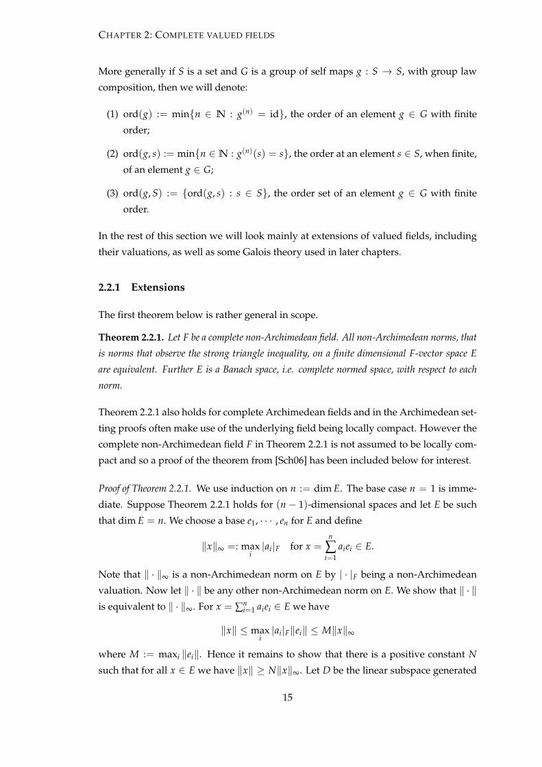
Proof of Theorem 2.2.1. We use induction on n := dim E. The base case n = 1 is imme-
diate. Suppose Theorem 2.2.1 holds for (n− 1)-dimensional spaces and let E be such
that dim E = n. We choose a base e1, · · · , en for E and define
‖x‖∞ =: maxi|ai|F for x =
n
∑i=1
aiei ∈ E.
Note that ‖ · ‖∞ is a non-Archimedean norm on E by | · |F being a non-Archimedean
valuation. Now let ‖ · ‖ be any other non-Archimedean norm on E. We show that ‖ · ‖is equivalent to ‖ · ‖∞. For x = ∑n
i=1 aiei ∈ E we have
‖x‖ ≤ maxi|ai|F‖ei‖ ≤ M‖x‖∞
where M := maxi ‖ei‖. Hence it remains to show that there is a positive constant N
such that for all x ∈ E we have ‖x‖ ≥ N‖x‖∞. Let D be the linear subspace generated
15

CHAPTER 2: COMPLETE VALUED FIELDS
by e1, · · · , en−1. By the inductive hypothesis there is c > 0 such that for all x ∈ D we
have ‖x‖ ≥ c‖x‖∞. Further D is complete and hence closed in E with respect to ‖ · ‖.Hence for
c′ := ‖en‖−1 inf{‖en − y‖ : y ∈ D}
we have 0 < c′ ≤ 1. Now set N := min(c′c, c′‖en‖) and let x ∈ E. Then x = y + anen
for some y ∈ D and an ∈ F. If an 6= 0 then ‖x‖ = |an|F‖en + a−1n y‖ ≥ |an|F‖en‖c′ =
c′‖anen‖. But then we also get
‖x‖ ≥ max(c′‖x‖, c′‖anen‖) ≥ c′‖x− anen‖ = c′‖y‖
and this inequality also holds for an = 0 since 0 < c′ ≤ 1. We get
‖x‖ ≥ c′max(‖y‖, ‖anen‖) ≥ c′max(c‖y‖∞, ‖en‖|an|F) ≥ N max(‖y‖∞, |an|F)
where N max(‖y‖∞, |an|F) = N‖x‖∞. Hence ‖ · ‖ and ‖ · ‖∞ are equivalent. Finally
we note that a sequence in E is a Cauchy sequence with respect to ‖ · ‖∞ if and only if
each of its coordinate sequences is a Cauchy sequence with respect to | · |F. Hence E is a
Banach space with respect to each norm by the equivalence of norms and completeness
of F.
Remark 2.2.2. Let L be a non-Archimedean field and let F be a complete subfield of L.
If L is a finite extension of F then L is also complete by Theorem 2.2.1. Now suppose L
is such a complete finite extension of F, then viewing L as a finite dimensional F-vector
space we note that convergence in L is coordinate-wise since | · |L is equivalent to ‖ · ‖∞
by Theorem 2.2.1. Hence each element g ∈ Gal(L/F) is continuous since being linear
over F. We will see later in this section that, for such complete finite extensions, each
element of Gal(L/F) is in fact an isometry. Finally in all cases if L is complete and g
is continuous then the fixed field Lg is also complete. To see this let (an) be a Cauchy
sequence in Lg and let a be its limit in L. For id the identity map on L, note that g− id
is also continuous on L and so Lg = (g− id)−1(0) is a closed subset of L. In particular
we have a ∈ Lg as required.
The following is Krull’s extension theorem, a proof can be found in [Sch06, p34].
Theorem 2.2.3. Let F be a subfield of a field L and let | · |F be a non-Archimedean valuation
on F. Then there exists a non-Archimedean valuation on L that extends | · |F.
The following corollary to Theorem 2.2.3, which also uses Theorem 2.1.4, contrasts with
the Archimedean setting.
Corollary 2.2.4. For every complete non-Archimedean field F there exists a proper extension
L of F for which the complete valuation on F extends to a complete valuation on L.
16
CHAPTER 2: COMPLETE VALUED FIELDS
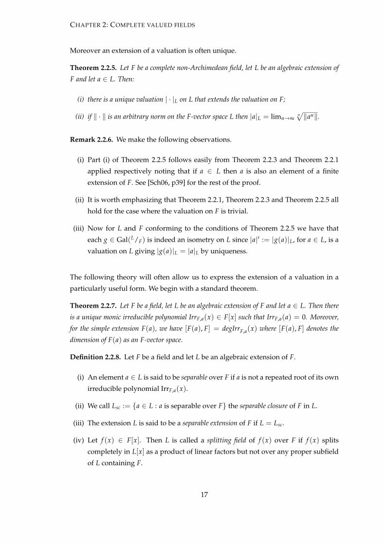
Moreover an extension of a valuation is often unique.
Theorem 2.2.5. Let F be a complete non-Archimedean field, let L be an algebraic extension of
F and let a ∈ L. Then:
(i) there is a unique valuation | · |L on L that extends the valuation on F;
(ii) if ‖ · ‖ is an arbitrary norm on the F-vector space L then |a|L = limn→∞n√‖an‖.
Remark 2.2.6. We make the following observations.
(i) Part (i) of Theorem 2.2.5 follows easily from Theorem 2.2.3 and Theorem 2.2.1
applied respectively noting that if a ∈ L then a is also an element of a finite
extension of F. See [Sch06, p39] for the rest of the proof.
(ii) It is worth emphasizing that Theorem 2.2.1, Theorem 2.2.3 and Theorem 2.2.5 all
hold for the case where the valuation on F is trivial.
(iii) Now for L and F conforming to the conditions of Theorem 2.2.5 we have that
each g ∈ Gal(L/F) is indeed an isometry on L since |a|′ := |g(a)|L, for a ∈ L, is a
valuation on L giving |g(a)|L = |a|L by uniqueness.
The following theory will often allow us to express the extension of a valuation in a
particularly useful form. We begin with a standard theorem.
Theorem 2.2.7. Let F be a field, let L be an algebraic extension of F and let a ∈ L. Then there
is a unique monic irreducible polynomial IrrF,a(x) ∈ F[x] such that IrrF,a(a) = 0. Moreover,
for the simple extension F(a), we have [F(a), F] = degIrrF,a(x) where [F(a), F] denotes the
dimension of F(a) as an F-vector space.
Definition 2.2.8. Let F be a field and let L be an algebraic extension of F.
(i) An element a ∈ L is said to be separable over F if a is not a repeated root of its own
irreducible polynomial IrrF,a(x).
(ii) We call Lsc := {a ∈ L : a is separable over F} the separable closure of F in L.
(iii) The extension L is said to be a separable extension of F if L = Lsc.
(iv) Let f (x) ∈ F[x]. Then L is called a splitting field of f (x) over F if f (x) splits
completely in L[x] as a product of linear factors but not over any proper subfield
of L containing F.
17

CHAPTER 2: COMPLETE VALUED FIELDS
(v) We will call L a normal extension of F if L is the splitting field over F of some
polynomial in F[x].
(vi) The field L is called a Galois extension of F if LG = F for G := Gal(L/F).
Remark 2.2.9. Following Definition 2.2.8 we note that the separable closure Lsc of F in
L is a field with F ⊆ Lsc ⊆ L. Moreover if F is of characteristic zero then L is a separable
extension of F.
For proofs of the following two theorems and Remark 2.2.9 see [McC66, p13-p19,p36].
Theorem 2.2.10. Let F be a field and let L be a finite extension of F. Then there is a normal
extension Lne of F which contains L and which is the smallest such extension in the sense that
if K is a normal extension of F which contains L then there is a L-monomorphism of Lne into K,
i.e. an embedding of Lne into K that fixes L.
Theorem 2.2.11. Let F be a field and let L be a finite extension of F. Then, with reference to
Theorem 2.2.10 and Definition 2.2.8, there are exactly [Lsc : F] distinct F-isomorphisms of L
onto subfields of Lne. Further if L = Lne then #Gal(L/F) = [Lsc : F]. Moreover L is a Galois
extension of F if and only if Lsc = L = Lne in which case #Gal(L/F) = [L : F].
Definition 2.2.12. Let F be a field, let L be a finite extension of F and let n0 := [Lsc : F].
By Theorem 2.2.11 there are exactly n0 distinct F-isomorphisms g1, · · · , gn0 of L onto
subfields of Lne. The norm map NL/F: L→ F is defined as
NL/F(a) :=
(n0
∏i=1
gi(a)
)[L:Lsc]
for a ∈ L.
A proof showing that the norm map only takes values in the ground field can be found
in [McC66, p23,p24]. Using the preceding theory we can now state and prove a theorem
that will often allow us to express the extension of a valuation in a particularly useful
form. The theorem is in the literature. However, having set out the preceding theory,
the proof presented here is more immediate than the sources I have seen.
Theorem 2.2.13. Let F be a complete non-Archimedean field with valuation |a|F = r−ν(a), for
a ∈ F, where ν is a valuation logarithm on F. Let L be a finite extension of F as a field. Then,
with reference to Theorem 2.2.5 and Theorem 2.2.1, the unique extension of | · |F to a complete
valuation | · |L on L is given by
|a|L = n√|NL/F
(a)|F = r−ω(a) for a ∈ L,
where n = [L : F] and ω := 1n ν ◦ NL/F
is the corresponding extension of ν to L. If in addition
the valuation | · |F is discrete then | · |L is also discrete. If further | · |F is non-trivial and ν is
the rank 1 valuation logarithm of remark 2.1.12 then eω(L×) = Z for some e ∈N.
18
CHAPTER 2: COMPLETE VALUED FIELDS
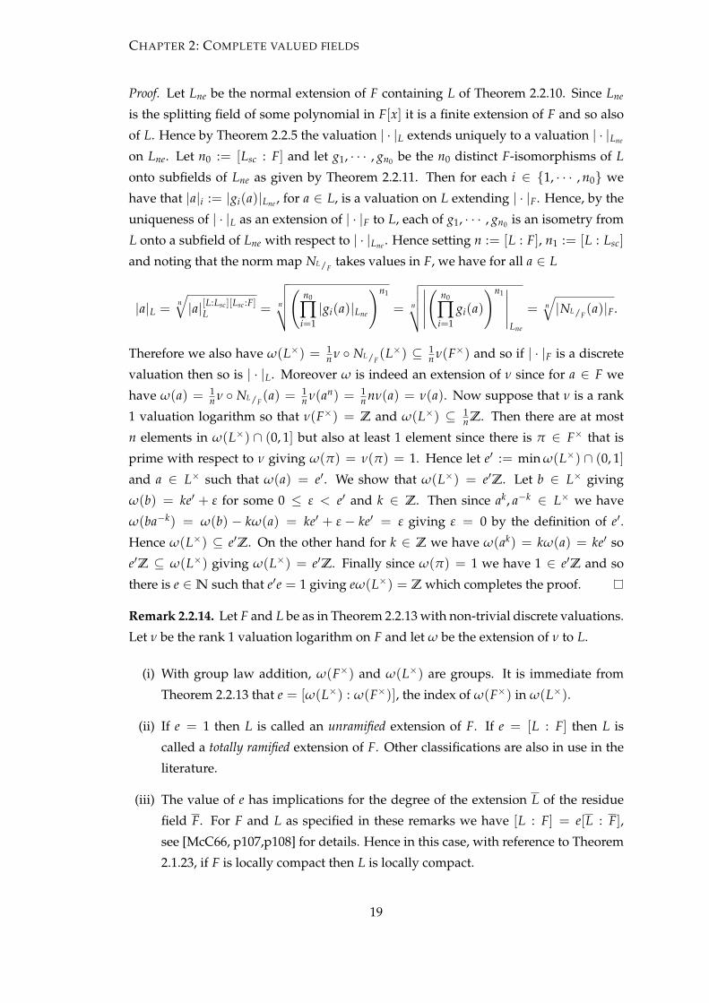
Proof. Let Lne be the normal extension of F containing L of Theorem 2.2.10. Since Lne
is the splitting field of some polynomial in F[x] it is a finite extension of F and so also
of L. Hence by Theorem 2.2.5 the valuation | · |L extends uniquely to a valuation | · |Lne
on Lne. Let n0 := [Lsc : F] and let g1, · · · , gn0 be the n0 distinct F-isomorphisms of L
onto subfields of Lne as given by Theorem 2.2.11. Then for each i ∈ {1, · · · , n0} we
have that |a|i := |gi(a)|Lne , for a ∈ L, is a valuation on L extending | · |F. Hence, by the
uniqueness of | · |L as an extension of | · |F to L, each of g1, · · · , gn0 is an isometry from
L onto a subfield of Lne with respect to | · |Lne . Hence setting n := [L : F], n1 := [L : Lsc]
and noting that the norm map NL/Ftakes values in F, we have for all a ∈ L
|a|L =n√|a|[L:Lsc][Lsc :F]
L = n
√√√√( n0
∏i=1|gi(a)|Lne
)n1
= n
√√√√∣∣∣∣∣(
n0
∏i=1
gi(a)
)n1∣∣∣∣∣
Lne
= n√|NL/F
(a)|F.
Therefore we also have ω(L×) = 1n ν ◦ NL/F
(L×) ⊆ 1n ν(F×) and so if | · |F is a discrete
valuation then so is | · |L. Moreover ω is indeed an extension of ν since for a ∈ F we
have ω(a) = 1n ν ◦ NL/F
(a) = 1n ν(an) = 1
n nν(a) = ν(a). Now suppose that ν is a rank
1 valuation logarithm so that ν(F×) = Z and ω(L×) ⊆ 1n Z. Then there are at most
n elements in ω(L×) ∩ (0, 1] but also at least 1 element since there is π ∈ F× that is
prime with respect to ν giving ω(π) = ν(π) = 1. Hence let e′ := min ω(L×) ∩ (0, 1]
and a ∈ L× such that ω(a) = e′. We show that ω(L×) = e′Z. Let b ∈ L× giving
ω(b) = ke′ + ε for some 0 ≤ ε < e′ and k ∈ Z. Then since ak, a−k ∈ L× we have
ω(ba−k) = ω(b) − kω(a) = ke′ + ε − ke′ = ε giving ε = 0 by the definition of e′.
Hence ω(L×) ⊆ e′Z. On the other hand for k ∈ Z we have ω(ak) = kω(a) = ke′ so
e′Z ⊆ ω(L×) giving ω(L×) = e′Z. Finally since ω(π) = 1 we have 1 ∈ e′Z and so
there is e ∈N such that e′e = 1 giving eω(L×) = Z which completes the proof.
Remark 2.2.14. Let F and L be as in Theorem 2.2.13 with non-trivial discrete valuations.
Let ν be the rank 1 valuation logarithm on F and let ω be the extension of ν to L.
(i) With group law addition, ω(F×) and ω(L×) are groups. It is immediate from
Theorem 2.2.13 that e = [ω(L×) : ω(F×)], the index of ω(F×) in ω(L×).
(ii) If e = 1 then L is called an unramified extension of F. If e = [L : F] then L is
called a totally ramified extension of F. Other classifications are also in use in the
literature.
(iii) The value of e has implications for the degree of the extension L of the residue
field F. For F and L as specified in these remarks we have [L : F] = e[L : F],
see [McC66, p107,p108] for details. Hence in this case, with reference to Theorem
2.1.23, if F is locally compact then L is locally compact.
19

CHAPTER 2: COMPLETE VALUED FIELDS
2.2.2 Galois theory
The following is the fundamental theorem of Galois theory, see [McC66, p36].
Theorem 2.2.15. Let F and E be fields such that E is a finite Galois extension of F, that is
EG = F for G := Gal(E/F). Then we have the following one-one correspondence
{G′ : G′ 6 G is a subgroup} ↔ {E′ : E′ is a field with F ⊆ E′ ⊆ E}
given by the inverse maps G′ 7→ EG′ and E′ 7→ Gal(E/E′).
Corollary 2.2.16. Let F and L be fields such that L is a finite extension of F and let G :=
Gal(L/F). Then L is a finite Galois extension of LG and so for L and LG Theorem 2.2.15 is
applicable.
Proof. We show that L is a Galois extension of LG. For g ∈ Gal(L/F) we have g(a) = a
for all a ∈ LG and so g ∈ Gal(L/LG). On the other hand for g ∈ Gal(L/LG) we have
g(a) = a for all a ∈ F since F ⊆ LG and so g ∈ Gal(L/F). Therefore Gal(L/F) =
Gal(L/LG) and so setting G′ := Gal(L/LG) gives LG′ = LG as required.
The following group theory result must be known. However we will provide a proof
in lieu of a reference.
Lemma 2.2.17. Let (G,+) be a group and g ∈ Aut(G) be a group automorphism on G. If
a, b ∈ G are such that gcd(ord(g, a), ord(g, b)) = 1 then ord(g, a + b) = ord(g, a)ord(g, b).
Proof. We assume the conditions of Lemma 2.2.17 and note that the result is imme-
diate if one or more of ord(g, a) and ord(g, b) is equal to 1. So assuming otherwise,
let pk11 pk2
2 · · · pkii and ql1
1 ql22 · · · q
ljj be the prime decompositions of ord(g, a) and ord(g, b)
respectively. For n := ord(g, a)ord(g, b) we have
g(n)(a + b) = g(n)(a) + g(n)(b) = a + b.
Therefore ord(g, a + b)|n. Suppose towards a contradiction that ord(g, a + b) < n.
Then ord(g, a + b)| nr for some r ∈ {p1, p2, · · · , pi, q1, q2, · · · , qj}. If r = pm for some
m ∈ {1, 2, · · · , i} then a + b = g(nr )(a + b) = g(
nr )(a) + g(
nr )(b) = g(
nr )(a) + b giving, by
right cancellation of b, g(nr )(a) = a. It then follows that
pk11 pk2
2 · · · pkmm · · · p
kii |p
k11 pk2
2 · · · pkm−1m · · · pki
i ql11 ql2
2 · · · qljj
giving pm|ql11 ql2
2 · · · qljj which is a contradiction since gcd(ord(g, a), ord(g, b)) = 1. A
similar contradiction occurs for r = qm with m ∈ {1, 2, · · · , j}. Hence ord(g, a + b) = n
as required.
20

CHAPTER 2: COMPLETE VALUED FIELDS
Lemma 2.2.18. Let F be a field with finite extension L and let g ∈ Gal(L/F). If n ∈N is such
that n|ord(g) then n ∈ ord(g, L).
Proof. Suppose towards a contradiction that there is n ∈ N such that n|ord(g) but
n /∈ ord(g, L). We can take n to be the least such element and note that n 6= 1 since
1 ∈ ord(g, L). Express n as n = pkr where p is a prime, k, r ∈N and p - r. We thus have
the following two cases.
Case: r 6= 1. In this case by the definition of n we have pk, r ∈ ord(g, L) and so there
are a, b ∈ L with ord(g, a) = pk, ord(g, b) = r and
gcd(ord(g, a), ord(g, b)) = 1.
Then by Lemma 2.2.17 we have ord(g, a + b) = ord(g, a)ord(g, b) which contradicts
our assumption that n /∈ ord(g, L).
Case: r = 1. In this case n = pk and note that ord(g) = nm for some m ∈N. Hence we
have the following subgroups of G:
(i) 〈g(n)〉 := ({id, g(n), g(2n), · · · , g((m−1)n)}, ◦) < G;
(ii) 〈g(np )〉 := ({id, g(
np ), g(2
np ), · · · , g((mp−1) n
p )}, ◦) 6 G.
Therefore #〈g(n)〉 = m, #〈g(np )〉 = mp and 〈g(n)〉 is a proper normal subgroup of 〈g(
np )〉.
Hence by Corollary 2.2.16 we have the following tower of fields
LG ⊆ L〈g(n/p)〉 $ L〈g
(n)〉 ⊆ L.
Now it is immediate that Lg(n) = L〈g(n)〉 and Lg(n/p)
= L〈g(n/p)〉 and so there is some
a ∈ Lg(n)\Lg(n/p)with ord(g, a)|n but ord(g, a) - n
p . Therefore ord(g, a) = pk = n which
again contradicts our assumption that n /∈ ord(g, L). In particular the lemma holds.
The following lemma is well known but we will provide a proof in lieu of a reference.
Lemma 2.2.19. Let F be a field, let L be an algebraic extension of F and let a ∈ L. For the
simple extension F(a) of F and F[X] the ring of polynomials over F we have F(a) = F[a].
Proof. It is immediate that F[a] ⊆ F(a). Now by Theorem 2.2.7 there is a unique monic
irreducible polynomial IrrF,a(x) ∈ F[X] such that IrrF,a(a) = 0. Further for any elementp(a)q(a) ∈ F(a), given by p(x), q(x) ∈ F[X], we have q(a) 6= 0. Hence IrrF,a(x) and q(x) are
relatively prime, that is we have gcd(IrrF,a, q) = 1. Therefore by Bezout’s identity there
are s(x), t(x) ∈ F[X] such that s(x)q(x) + t(x)IrrF,a(x) = 1 giving q(x) = 1−t(x)IrrF,a(x)s(x) .
Finally then we have q(a) = 1s(a) giving p(a)
q(a) = p(a)s(a) which is an element of F[a] as
required.
21

CHAPTER 3
Functions and algebras
In this chapter we build upon some of the basic facts and analysis of complete valued
fields surveyed in Chapter 2. The first section establishes particular facts in functional
analysis over complete valued fields that will be used in later chapters. However it is
not the purpose of the first section to provide an extensive introduction to the subject.
The second section provides background on Banach F-algebras, Banach algebras over a
complete valued field F. Whilst some of the details are included purely as background
others also support the discussion from Remark 2.1.17 of Chapter 2.
3.1 Functional analysis over complete valued fields
We begin with the following lemma.
Lemma 3.1.1. Let F be a non-Archimedean field and let (an) be a sequence of elements of F.
(i) If limn→∞ an = a for some a ∈ F× then there exists N ∈ N such that for all n ≥ N we
have |an|F = |a|F. We will call this convergence from the side, opposed to from above
or below.
(ii) If F is also complete then ∑ an converges if and only if limn→∞ an = 0, in sharp contrast
to the Archimedean case. Further if ∑ an does converge then∣∣∑ an∣∣
F ≤ max{|an|F : n ∈N}.
Proof. For (i), since a 6= 0 we have |a|F > 0 and so there is some N ∈ N such that,
for all n ≥ N, |an − a|F < |a|F. Hence for all n ≥ N we have by Lemma 2.1.7 that
|an|F = |(an − a) + a|F = |a|F.
For (ii), suppose limn→∞ an = 0 and let ε > 0. Then there is N ∈ N such that for all
22

CHAPTER 3: FUNCTIONS AND ALGEBRAS
n ≥ N we have |an|F < ε. Hence for n1, n2 ∈N with N < n1 < n2 we have∣∣∣∣∣ n2
∑i=1
ai −n1
∑i=1
ai
∣∣∣∣∣F
=
∣∣∣∣∣ n2
∑i=n1+1
ai
∣∣∣∣∣F
≤ max{|an1+1|F, · · · , |an2 |F} < ε.
Hence the sequence of partial sums is a Cauchy sequence in F and so converges. The
converse is immediate. Further suppose ∑ an does converge. For ∑ an 6= 0 we have by
(i) that there is N ∈N such that for all n ≥ N∣∣∣∣∣ ∞
∑i=1
ai
∣∣∣∣∣F
=
∣∣∣∣∣ n
∑i=1
ai
∣∣∣∣∣F
≤ max{|a1|F, · · · , |an|F} ≤ max{|ai|F : i ∈N}.
On the other hand for ∑ an = 0 the result is immediate.
The following theorem appears in [Sch06, p59] without proof.
Theorem 3.1.2. Let F be a complete non-Archimedean field and let a0, a1, a2, · · · be a sequence
of elements of F. Define the radius of convergence by
ρ :=1
lim supn→∞n√|an|F
where by convention 0−1 = ∞ and ∞−1 = 0.
Then the power series ∑ anxn, x ∈ F, converges if |x|F < ρ and diverges if |x|F > ρ. Further-
more for each t ∈ (0, ∞), t < ρ the convergence is uniform on Bt(0) := {a ∈ F : |a|F ≤ t}.
Proof. Note that the following equalities hold, except for when |x|F = ρ = 0,
lim supn→∞
n√|anxn|F = lim sup
n→∞
n√|an|F|x|nF =
|x|Fρ
. (3.1.1)
Suppose ∑ anxn is divergent. Then by part (ii) of Lemma 3.1.1, limn→∞ anxn is not 0.
Therefore there is some ε ∈ (0, 1] such that for each m ∈ N there is n > m with
|anxn|F ≥ ε, in particular n√|anxn|F ≥ n
√ε ≥ m√
ε. Hence since limm→∞m√
ε = 1 we have
lim supn→∞n√|anxn|F ≥ 1. Therefore in this case |x|F ≥ ρ by (3.1.1). In particular for
cases where |x|F < ρ the series ∑ anxn converges.
On the other hand suppose ∑ anxn converges. Then since limn→∞ |anxn|F = 0 we have
lim supn→∞n√|anxn|F ≤ lim supn→∞
n√
12 = 1. Therefore in this case |x|F ≤ ρ by (3.1.1).
In particular for cases where |x|F > ρ the series ∑ anxn diverges.
Now suppose there is t ∈ (0, ∞) with t < ρ and let ε > 0. If the valuation on F
is dense then |F×|F is dense in the positive reals and so there is some x0 ∈ F× with
t < |x0|F < ρ. Alternatively, if the valuation on F is discrete, there is x0 ∈ Bt(0) with
|x0|F = max{|a|F : a ∈ Bt(0)}. In either case, since |x0|F < ρ, ∑ anxn0 converges and
so limn→∞ anxn0 = 0. Hence there is some N ∈ N such that for all n > N we have
23

CHAPTER 3: FUNCTIONS AND ALGEBRAS
|anxn0 |F < ε. Now by the last part of Lemma 3.1.1 we have for all m > N and x ∈ Bt(0)
that
|∞
∑n=1
anxn −m
∑n=1
anxn|F = |∞
∑n=m+1
anxn|F ≤ max{|anxn|F : n ≥ m + 1}.
But |anxn|F = |an|F|x|nF ≤ |an|F|x0|nF = |anxn0 |F and so max{|anxn|F : n ≥ m + 1} < ε
and the convergence is uniform on Bt(0).
Remark 3.1.3. With reference to Theorem 3.1.2.
(i) We note that the radius of convergence as defined in Theorem 3.1.2 is the same as
that used in the Archimedean setting when replacing F with the complex num-
bers. However, unlike in the complex setting, if the valuation on F is discrete
then a power series ∑ anxn may not have a unique choice for the definition of its
radius of convergence since |F×|F is discrete in this case.
(ii) We need to be careful when considering convergence of power series. Let | · |∞denote the absolute valuation on R and let | · |0 denote the trivial valuation on
R. All power series are convergent on B1(0) := {a ∈ R : |a|0 < 1} = {0} with
respect to | · |0. Whereas the only power series that are convergent at a point a ∈R× with respect to | · |0 are polynomials. On the other hand exp(x) := ∑∞
n=1xn
n!
converges everywhere on R with respect to | · |∞. The function exp(x) defined
with respect to | · |∞ is a continuous function on all of R with respect to | · |0 but
does not have a power series representation on R with respect to | · |0. Similarly
∑∞n=1
xn
n! does not converge everywhere on the p-adic numbers Qp with respect to
| · |p, see [Sch06, p70] for details in this case.
(iii) Under the conditions of Theorem 3.1.2, suppose that the ball Bρ(0) is without
isolated points where ρ is the radius of convergence of f (x) := ∑ anxn. Then,
with differentiation defined as in the Archimedean setting, the derivative of f
exists on Bρ(0) and it is f ′(x) = ∑ nanxn−1. We will not consider this in depth
but note, for x ∈ Bρ(0), the series ∑ anxn converges giving limn→∞ cn = 0 for
cn := anxn by Lemma 3.1.1. Hence for all n ∈ N, since |n|F = |11 + · · ·+ 1n|F ≤max{|11|F, · · · , |1n|F} = 1, we have for x 6= 0 that
|nanxn−1|F = |n|F|x−1|F|anxn|F ≤ |x−1|F|cn|F.
Therefore the series ∑ nanxn−1 also converges on Bρ(0) by Lemma 3.1.1.
3.1.1 Analytic functions
Let F be a complete valued field. In this subsection we consider F valued functions
that are analytic on the interior of some subset of F that is without isolated points. In
24

CHAPTER 3: FUNCTIONS AND ALGEBRAS
particular the situation concerning such analytic functions is some what different in the
non-Archimedean setting to that in the Archimedean one, even though the standard re-
sults of differentiation such as the chain rule and Leibniz rule are the same, see [Sch06,
p59]. Recall that if a complex valued function f is analytic on an open disc Dr(a) ⊆ C
then f can be represented by the convergent power series
f (z) =∞
∑n=0
f (n)(a)n!
(z− a)n for z ∈ Dr(a),
known as the Taylor expansion of f about a, where f (n)(a) is the nth derivative of f at a.
Moreover if b ∈ Dr(a) then f can also be expanded about b. However this expansion
need not be convergent on all of Dr(a) merely on the largest open disc centered at b
contained in Dr(a) since a lack of differentiability of f at points on, or outside, the
boundary of Dr(a) will restrict the radius of convergence of such an expansion, see
[Apo74, p449,p450].
Now for F a complete non-Archimedean field the same scenario in this case is such
that if f is analytic on a ball Br(a) ⊆ F and can be represented by a Taylor expansion
about a on all of Br(a) then f can be represented by a Taylor expansion about any other
point b ∈ Br(a) and this expansion will also be valid on all of Br(a), see [Sch06, p68].
This is closely related to the fact that every point of Br(a) is at its center, see the proof
of Lemma 2.1.20. However in general a function f analytic on Br(a) ⊆ F need not have
a Taylor expansion about a that is valid on all of Br(a). This is because Br(a) can be
decomposed as a disjoint union of clopen balls, see Remark 2.1.21, upon each of which
f can independently be defined. This leads to the following definitions.
Definition 3.1.4. Let F be a complete valued field with non-trivial valuation.
(i) We will call a subset X ⊆ F strongly convex if X is either F, the empty set ∅, a ball
or a singleton set.
(ii) Let X be an open strongly convex subset of F and let f : X → F be a continuous
F-valued function on X. If f can be represented by a single Taylor expansion that
is valid on all of X then we say that f is globally analytic on X.
(iii) Let X be an open subset of F and let f : X → F be a continuous F-valued function
on X. If for each a ∈ X there is an open strongly convex neighborhood V ⊆ X of
a such that f |V is globally analytic on V then we say that f is locally analytic on X.
(iv) Let X and f be as in (iii). As usual, if the derivative
f ′(a) := limx→a
f (x)− f (a)x− a
exists at every a ∈ X then we say that f is analytic on X.
25

CHAPTER 3: FUNCTIONS AND ALGEBRAS
(v) In the case where X = F we similarly define globally entire, locally entire and entire
functions on X.
Remark 3.1.5. Note that the condition in Definition 3.1.4 that F has a non-trivial valua-
tion is there because it does not make sense to talk about analytic functions defined on
a space without accumulation points. We also note that (ii), (iii) and (iv) of Definition
3.1.4 are equivalent in the complex setting for X an open strongly convex subset of C,
see [Apo74, p450].
Now let F be a complete non-Archimedean field and let ( fn) be a sequence of F-valued
functions analytic on B1(0) and converging uniformly on B1(0) to a function f . We
ask whether f will also be analytic on B1(0) in this case? It is very well known that the
answer to the analog of this question involving the complex numbers is yes although in
this case the functions are required to be continuous on B1(0) and analytic only on the
interior of B1(0) since B1(0) will not be clopen. In the case involving the real numbers
the answer to the question is of course no since for example a function with a chevron
shaped graph in R2 can be uniformly approximated by differentiable functions. In the
non-Archimedean setting the following theorem provides insight for when F is not
locally compact and also gives a maximum principle result, see [Sch06, p122] for proof.
Theorem 3.1.6. Let F be a complete non-Archimedean field that is not locally compact and let
r ∈ |F×|F.
(i) If f1, f2, · · · are globally analytic functions on Br(0) and if f := limn→∞ fn uniformly
on Br(0) then f is also globally analytic on Br(0).
(ii) Let f be a globally analytic function on Br(0) with power series f (x) = ∑∞n=0 anxn.
If the valuation | · |F is dense then
sup{| f (x)|F : |x|F ≤ r} = sup{| f (x)|F : |x|F < r} = max{|an|Frn : n ≥ 0} < ∞.
If the residue field F is infinite then
max{| f (x)|F : |x|F ≤ r} = max{| f (x)|F : |x|F = r} = max{|an|Frn : n ≥ 0} < ∞.
Remark 3.1.7. In Theorem 3.1.6 Br(0) is not compact since F is not locally compact. In
fact every ball of positive radius is not compact in this case and this follows from Theo-
rem 2.1.23 noting that translations and non-zero scalings in F are homeomorphisms on
F. Now since we are progressing towards a study of uniform algebras and their gen-
eralisation over complete valued fields we note that in order to use the uniform norm,
see Remark 4.1.2, on such algebras of continuous functions we need the functions to be
bounded. Hence to avoid imposing boundedness directly it is convenient to work on
compact spaces.
26

CHAPTER 3: FUNCTIONS AND ALGEBRAS
For B1(0) compact, i.e. in the F locally compact case, I provide the following example to
show that in this case the uniform limit of locally analytic, and hence analytic, functions
on B1(0) need not be analytic.
Example 3.1.8. Let F be a locally compact, complete non-Archimedean field with non-
trivial valuation. Then we have the following sequence of functions on B1(0) ⊆ F,
fn(x) :=
{πν(x) if ν(x) < n
0 if ν(x) ≥ nfor x ∈ B1(0)
where π is a prime element of F and ν is the rank 1 valuation logarithm. For each n ∈N, fn is a locally constant function since convergence in F is from the side, see Lemma
3.1.1, and so fn is locally analytic on B1(0). Moreover the sequence ( fn) converges
uniformly on B1(0) to the continuous function
f (x) :=
{πν(x) if x 6= 0
0 if x = 0for x ∈ B1(0)
with limx→0 f (x) = 0 since | f (x)|F = |x|F for all x ∈ B1(0). We now show that f is not
differentiable at zero. let a1, a2, · · · and b1, b2, · · · be sequences in F given by an := πn
and bn := −πn. Both of these sequences tend to zero as n tends to ∞. But then
f (an)− f (0)an
= (πn − 0)π−n = 1 andf (bn)− f (0)
bn= (πn − 0)(−π−n) = −1
for all n ∈ N so that the limit limx→0f (x)− f (0)
x does not exist as required. Alternatively
we can obtain a similar example by redefining f as
f (x) :=
π
12 ν(x) if ν(x) is even
π12 (ν(x)−1) if ν(x) is odd
0 if x = 0
for x ∈ B1(0).
In this case limx→0f (x)− f (0)
x blows up with respect to | · |F as demonstrated by the se-
quence c1, c2, · · · with cn := π2n.
Later when we look at non-complex analogs of uniform algebras we will see, from Ka-
plansky’s non-Archimedean generalisation of the Stone-Weierstrass theorem, that the
continuous functions in Example 3.1.8 can be uniformly approximated by polynomials
on B1(0) given that B1(0) is compact in this case. Hence Example 3.1.8 also shows that,
for F locally compact, the uniform limit of globally analytic functions on B1(0) need
not be analytic in contrast to Theorem 3.1.6.
In anticipation of topics in the next section we now consider Liouville’s theorem. It is
immediate that the standard Liouville theorem never holds in the non-Archimedean
27
CHAPTER 3: FUNCTIONS AND ALGEBRAS
setting since for a complete non-Archimedean field F with non-trivial valuation the in-
dicator function χB for B := B1(0) is a non-constant bounded locally analytic function
from F to F noting that B1(0) is a clopen subset of F. However the following is called
the ultrametric Liouville theorem.
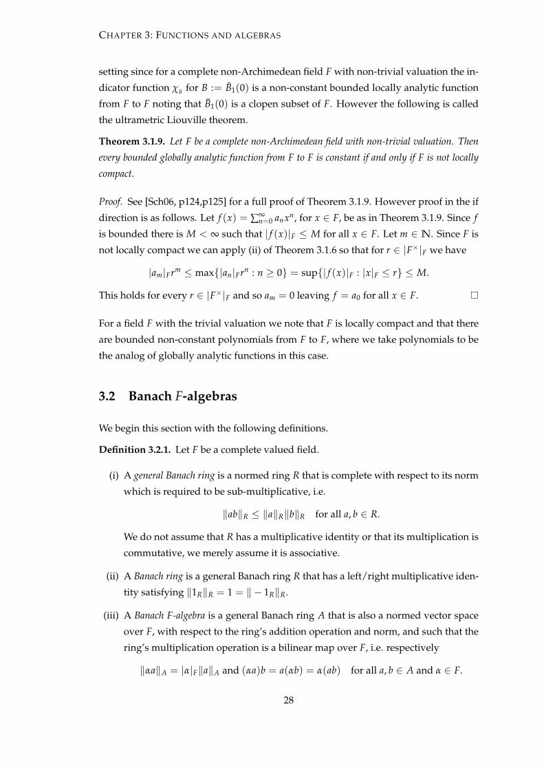
Theorem 3.1.9. Let F be a complete non-Archimedean field with non-trivial valuation. Then
every bounded globally analytic function from F to F is constant if and only if F is not locally
compact.
Proof. See [Sch06, p124,p125] for a full proof of Theorem 3.1.9. However proof in the if
direction is as follows. Let f (x) = ∑∞n=0 anxn, for x ∈ F, be as in Theorem 3.1.9. Since f
is bounded there is M < ∞ such that | f (x)|F ≤ M for all x ∈ F. Let m ∈ N. Since F is
not locally compact we can apply (ii) of Theorem 3.1.6 so that for r ∈ |F×|F we have
|am|Frm ≤ max{|an|Frn : n ≥ 0} = sup{| f (x)|F : |x|F ≤ r} ≤ M.
This holds for every r ∈ |F×|F and so am = 0 leaving f = a0 for all x ∈ F.
For a field F with the trivial valuation we note that F is locally compact and that there
are bounded non-constant polynomials from F to F, where we take polynomials to be
the analog of globally analytic functions in this case.
3.2 Banach F-algebras
We begin this section with the following definitions.
Definition 3.2.1. Let F be a complete valued field.
(i) A general Banach ring is a normed ring R that is complete with respect to its norm
which is required to be sub-multiplicative, i.e.
‖ab‖R ≤ ‖a‖R‖b‖R for all a, b ∈ R.
We do not assume that R has a multiplicative identity or that its multiplication is
commutative, we merely assume it is associative.
(ii) A Banach ring is a general Banach ring R that has a left/right multiplicative iden-
tity satisfying ‖1R‖R = 1 = ‖ − 1R‖R.
(iii) A Banach F-algebra is a general Banach ring A that is also a normed vector space
over F, with respect to the ring’s addition operation and norm, and such that the
ring’s multiplication operation is a bilinear map over F, i.e. respectively
‖αa‖A = |α|F‖a‖A and (αa)b = a(αb) = α(ab) for all a, b ∈ A and α ∈ F.
28

CHAPTER 3: FUNCTIONS AND ALGEBRAS
(iv) A unital Banach F-algebra is a Banach F-algebra that is also a Banach ring opposed
to being merely a general Banach ring.
(v) By commutative general Banach ring and commutative Banach F-algebra etc. we mean
that the multiplication is commutative in these cases. By F-algebra we mean the
structure of a Banach F-algebra but without the requirement of a norm.
Remark 3.2.2. In Definition 3.2.1 we always require a multiplicative identity to be dif-
ferent to the additive identity. As standard we will usually dispense with the sub-
script when denoting elements of the structures defined in Definition 3.2.1 and in the
Archimedean setting we will call a Banach C-algebra a complex Banach algebra and a
Banach R-algebra a real Banach algebra.
3.2.1 Spectrum of an element
The following discussion concerns the spectrum of an element.
Definition 3.2.3. Let F be a complete valued field and let A be a unital Banach F-
algebra. Then for a ∈ A we call the set
Sp(a) := {λ ∈ F : λ− a is not invertible in A}
the spectrum of a.
Theorem 3.2.4. Every element of every unital complex Banach algebra has non-empty spec-
trum.
Theorem 3.2.4 is very well known. A proof can be found in [Sto71, p11] and relies
on Liouville’s theorem and the Hahn-Banach theorem in the complex setting. We will
confirm that this result is unique among unital Banach F-algebras and I will give details
of where the proof from the complex setting fails for other complete valued fields.
Let us first recall the Gelfand-Mazur theorem which demonstrates the importance of
Theorem 3.2.4 in the complex setting and supports Remark 2.1.17 of Chapter 2.
Theorem 3.2.5. A unital complex Banach algebra that is also a division ring is isometrically
isomorphic to the complex numbers.
Proof. Let A be a unital complex Banach algebra that is also a division ring and let
a ∈ A. Since in this case Sp(a) is non-empty, there is some λ ∈ Sp(a). Hence because
A is a division ring λ − a = 0 giving a = λ. More accurately we have a = λ1A but
because A is unital we have ‖a‖A = ‖λ1A‖A = |λ|∞‖1A‖A = |λ|∞ and so the map
from A onto C given by λ1A 7→ λ is an isometric isomorphism.
29

CHAPTER 3: FUNCTIONS AND ALGEBRAS
Remark 3.2.6. In the Archimedean setting it follows immediately from Theorem 3.2.5
that any complete valued field containing the complex numbers as a valued subfield
will coincide with the complex numbers. Note that the proof of Theorem 3.2.5 is very
well known.
In contrast to Theorem 3.2.4 we have the following lemma. The result is certainly
known but we give full details in lieu of a reference.
Lemma 3.2.7. Let F be a complete valued field other than the complex numbers. Then there
exists a unital Banach F-algebra A such that Sp(a) = ∅ for some a ∈ A.
Proof. Let F be a complete valued field other that the complex numbers. By Corollary
2.2.4 in the non-Archimedean setting, and since R is the only complete valued field
other than C in the Archimedean setting, we can always find a complete valued field L
that is a proper extension of F. Let a ∈ L\F and note that L is a unital Banach F-algebra.
Then for every λ ∈ F we have λ− a 6= 0 and so λ− a is invertible in L since L is a field.
Hence Sp(a) = ∅.
Whilst not considering every case, we now consider where the proof of Theorem 3.2.4
fails when applying it to unital Banach F-algebras with F 6= C. For F = R the Hahn-
Banach theorem holds but Liouville’s theorem does not with the trigonometric sin func-
tion restricted to R as an example of a non-constant, bounded, analytic function from
R to R. In the non-Archimedean setting we do have the ultrametric Liouville theorem,
Theorem 3.1.9 for F not locally compact, and there is also an ultrametric Hahn-Banach
theorem for spherically complete fields, as follows.
Definition 3.2.8. An ultrametric space, see Definition 2.1.1, is spherically complete if each
nested sequence of balls has a non-empty intersection.
Theorem 3.2.9. Let F be a spherically complete non-Archimedean field and let V be an F-vector
space, s a seminorm on V and V0 ⊆ V a vector subspace. Then for every linear functional
`0 : V0 → F such that |`0(v)|F ≤ s(v) for all v ∈ V0 there is a linear functional ` : V → F
such that `|V0 = `0 and |`(v)|F ≤ s(v) for all v ∈ V.
Remark 3.2.10. We note that Theorem 3.2.9 is exactly the same as the Hahn-Banach
theorem from the Archimedean setting, see [Sto71, p472], except with R and C replaced
by any spherically complete non-Archimedean field. A proof can be found in both
[Sch02, p51] and [Sch06, p288] the latter of which further states that Theorem 3.2.9
becomes a falsity if F is replaced by a non-spherically complete field. It is immediate
that spherically complete ultrametric spaces are complete.
A proof of the following lemma can be found in [Sch02, p6].
30
CHAPTER 3: FUNCTIONS AND ALGEBRAS
Lemma 3.2.11. All complete non-Archimedean fields with a discrete valuation are spherically
complete. In particular if F is a complete non-Archimedean fields that is locally compact then F
is spherically complete.
From the above details we see that for both Theorem 3.1.9 and Theorem 3.2.9 to be ap-
plicable we need a non-locally compact, spherically complete, non-Archimedean field.
This restricts the possibilities since for example, for any prime p, a finite extension of
Qp is locally compact and Cp whilst not locally compact is also not spherically com-
plete, see [Sch02, p5]. However, with reference to (ii) of Example 2.1.15, the complete
non-Archimedean field C{{T}} is not locally compact since having an infinite residue
field and it is spherically complete since its valuation is discrete. Moreover the totally
ramified, see Remark 2.2.14, simple extension C{{T}}(√
T) is a unital Banach C{{T}}-algebra with complete valuation given by Theorem 2.2.13. But by the proof of Lemma
3.2.7 we have Sp(√
T) = ∅. So let’s briefly review how the proof of Theorem 3.2.4 from
[Sto71, p11] works and then consider where it fails for C{{T}}(√
T).
Let A be a unital complex Banach algebra and let a ∈ A. Suppose towards a contra-
diction that Sp(a) = ∅. Then λ− a is invertible for all λ ∈ C. In particular a−1 exists
in A and the map `0 : Ca−1 → C, given by `0(λa−1) := λα for a fixed α ∈ C with
0 < |α|∞ ≤ ‖a−1‖A, is a continuous linear functional on the subspace Ca−1 of A to
which the Hahn-Banach theorem can be applied directly. Hence there exists a continu-
ous linear functional ` : A → C such that `(−a−1) = −α 6= 0. On the other hand for
any continuous linear functional ϕ : A→ C we can define a function fϕ : C→ C by
fϕ(λ) := ϕ((λ− a)−1).
The proof then shows that fϕ is differentiable at every point of C and is therefore an
entire function. Moreover limλ→∞ fϕ(λ) = 0 since
| fϕ(λ)|∞ =
∣∣∣∣ 1λ
ϕ((1− λ−1a)−1)
∣∣∣∣∞≤ 1|λ|∞‖ϕ‖op‖(1− λ−1a)−1‖A,
where ‖ · ‖op is the standard operator norm. Hence, by Liouville theorem in the com-
plex setting, fϕ is the zero function. But we have f`(0) = −α 6= 0, a contradiction, and
so Sp(a) 6= ∅ as required. Note however that the function fϕ is defined on C\Sp(a).
Now for C{{T}}(√
T) the coordinate projection P : C{{T}}(√
T)→ C{{T}} given by
P(α + β√
T) := α, where α, β ∈ C{{T}}, is a continuous linear functional analogous
to an evaluation functional noting that convergence in C{{T}}(√
T) is coordinate-wise
over C{{T}} by Remark 2.2.2. Hence we can define a function fP : C{{T}} → C{{T}}given by
fP(λ) := P((λ−√
T)−1) = P((λ +√
T)(λ2 − T)−1) = λ(λ2 − T)−1.
31
CHAPTER 3: FUNCTIONS AND ALGEBRAS
The function fP is defined on all of C{{T}} since the roots of λ2− T are√
T and −√
T.
Furthermore fP is not constant and so it is the relative weakness of the ultrametric
Liouville theorem in the non-Archimedean setting that allows the argument used in
the proof of Theorem 3.2.4 to fails in this case. Indeed we will now show that fP is not
globally analytic on all of C{{T}}. The first derivative of fP is
f (1)P (λ) = (λ2 − T)−1 − 2λ2(λ2 − T)−2
and so fP(0) = 0 and f (1)P (0) = − 1T . Continuing in this way we obtain the Taylor
expansion of fP about zero as
fP(λ) =∞
∑n=0
αnλn = −(
λ
T+
λ3
T2 +λ5
T3 +λ7
T4 + · · ·)
, for |λ|T < ρ,
where αn := f (n)P (0)n! = − 1−(−1)n
2 T−12 (1+n) ∈ C{{T}} and
ρ =1
lim supn→∞n√|αn|T
is the radius of convergence of the Taylor series expansion. Hence we show that ρ
is finite. Using the rank 1 valuation logarithm, for ∑n∈Z anTn ∈ C{{T}}× we have
|∑n∈Z anTn|T = r−min{n:an 6=0} for some fixed r > 1. Hence, noting that α2n = 0 and
α2n−1 = −T−n for n ∈N, we have
lim supn→∞
n√|αn|T = lim
n→∞2n−1√|α2n−1|T = lim
n→∞
2n−1√
rn = limn→∞
rn
2n−1 = r12 .
Hence ρ = 1√r < 1 since r > 1. In particular fP is only locally analytic on C{{T}}
and not globally analytic, consistent with the ultrametric Liouville theorem not being
applicable to fP as required.
Definition 3.2.12. Let F be a complete valued field and let A be a unital Banach F-
algebra. Define F (A) as the set of all complete valued fields L contained inside A over
which A is also a unital Banach L-algebra.
Remark 3.2.13. Concerning the spectrum of an element.
(i) It is tempting to conjecture that a generalisation of Theorem 3.2.4 might hold for
every complete valued field F provided that, given F, we restrict the statement
to those unital Banach F-algebras A for which F is a maximal element of F (A).
This conjecture is false in both the non-commutative and commutative settings
by Lemma 3.2.14 below. However for a more general version of the conjecture
one could permit the elements of F (A) to be complete normed division rings.
32
CHAPTER 3: FUNCTIONS AND ALGEBRAS
(ii) Let A be a unital real Banach algebra. In order to avoid an element a ∈ A having
empty spectrum Kaplansky gave the following alternative definition in this case,
SpK(a) := {α + iβ ∈ C : (a− α)2 + β2 is not invertible in A}.
We won’t investigate this definition here but for more details see [KL92, p6].
Lemma 3.2.14. In both the non-commutative and commutative algebra settings one can find
a complete valued field F, a unital Banach F-algebra A and an element a ∈ A such that F is a
maximal element of F (A) and Sp(a) = ∅.
Proof. Hamilton’s real quaternions, H, are an example of a non-commutative complete
Archimedean division ring and unital real Banach algebra. Viewing H as a real vec-
tor space, the valuation on H is the Euclidean norm which is complete, Archimedean
and indeed a valuation since being multiplicative on H, see [Lam05, p56,p57]. By the
Gelfand-Mazur theorem, Theorem 3.2.5, H is not a unital complex Banach algebra since
being different to C and so R is maximal in F (H). Moreover for a ∈ H\R it is imme-
diate that we have Sp(a) = ∅.
In the commutative setting consider the field of complex numbers C with the absolute
valuation replaced by the L1-norm as it applies to the real vector space R2, that is for
a = α + iβ ∈ C we have ‖a‖1 := |α|∞ + |β|∞. Then C is complete with respect to ‖ · ‖1
by the equivalence of norms on finite dimensional R-vector spaces. Expressing com-
plex numbers in their coordinate form it is easy to show that ‖ · ‖1 is sub-multiplicative
and so (C, ‖ · ‖1) is a unital real Banach algebra. However ‖ · ‖1 is not multiplicative
since ‖(1 + i)(1− i)‖1 = ‖2‖1 = 2 < 4 = ‖1 + i‖1‖1− i‖1 and so ‖ · ‖1 is not a valua-
tion on C. Consequently R is maximal in F ((C, ‖ · ‖1)) and over R, Sp(i) = ∅ which
completes the proof.
33

CHAPTER 4
Uniform algebras
In the first section of this chapter we survey some of the basic facts about complex
uniform algebras and recall the close connection with the study of compact Hausdorff
spaces, such as Swiss cheese sets, upon which such algebras of functions are defined.
An inductive proof by the author of the Feinstein-Heath Swiss cheese “classicalisa-
tion” theorem is then presented. An article containing this proof has been published
by the American Mathematical Society, see [Mas10]. In the second section of this chap-
ter we turn our attention to non-complex analogs of uniform algebras. The constraints
imposed by the various generalisations of the Stone-Weierstrass theorem are consid-
ered and the theory of real function algebras developed by Kulkarni and Limaye is
introduced. We will establish the topological requirements of the spaces upon which
algebras of functions in the non-Archimedean setting can be defined whilst qualifying
as non-complex analogs of uniform algebras. These observations together with some
of the details and examples from other chapters have been gathered together by the
author into a survey paper which was subsequently accepted for publication by the
American Mathematical Society, see [Mas11].
4.1 Complex uniform algebras
Definition 4.1.1. Let CC(X) be the unital complex Banach algebra of all continuous
complex valued functions, defined on a compact Hausdorff space X, with pointwise
operations and the sup norm given by
‖ f ‖∞ := supx∈X| f (x)|∞ for all f ∈ CC(X).
A uniform algebra, A, is a subalgebra of CC(X) that is complete with respect to the sup
norm, contains the constant functions making it a unital complex Banach algebra and
separates the points of X in the sense that for all x1, x2 ∈ X with x1 6= x2 there is f ∈ A
satisfying f (x1) 6= f (x2).
34
CHAPTER 4: UNIFORM ALGEBRAS
Remark 4.1.2. Introductions to uniform algebras can be found in [Bro69], [Gam69] and
[Sto71]. Some authors take Definition 4.1.1 to be a representation of uniform algebras
and take a uniform algebra A to be a unital complex Banach algebra with a square
preserving norm, that is ‖a2‖ = ‖a‖2 for all a ∈ A, which they sometimes then referred
to as a uniform norm. This is quite legitimate since, as we will discuss at depth in
the section on representation theory, the Gelfand transform shows us that every such
algebra is isometrically isomorphic to an algebra conforming to Definition 4.1.1. In this
thesis we mainly introduce generalisations of Definition 4.1.1 over complete valued
fields and then investigate the important representation theory results. Hence for us
by uniform norm we will mean the sup norm.
It is very well known that in the complex setting, for suitable X, there exist uniform
algebras that are proper subalgebras of CC(X). However if A is such a uniform algebra
then A is not self-adjoint, that is there is f ∈ A with f /∈ A where f denotes the complex
conjugate of f . This result is the complex Stone-Weierstrass theorem, generalisations of
which we will meet in Section 4.2. We will also meet several analogs of the following
example.
Example 4.1.3. A standard example is the disc algebra A(∆) ⊆ CC(∆), of continuous
functions analytic on the interior of ∆ := {z ∈ C : |z| ≤ 1}, which is as far from
being self-adjoint as possible since if both f and f are in A(∆) then f is constant, see
[KL92, p47]. Also P(∆) = A(∆) where P(∆) is the uniform algebra of all functions on
∆ that can be uniformly approximated by polynomials restricted to ∆ with complex
coefficients. This largely follows from Remark 3.1.5, see [Bro69, p5] or [Sto71, p2].
For a compact Hausdorff space X let R(X) denote the uniform algebra of all functions
on X that can be uniformly approximated by rational functions from CC(X). We also
generalise to X the uniform algebras introduced in Example 4.1.3 giving A(X) and
P(X). In the theory of uniform approximation it is standard to ask for which X is one
or more of the following inclusions non-trivial
P(X) ⊆ R(X) ⊆ A(X) ⊆ CC(X).
Whilst not always the case, this often only depend on X up to homeomorphism. In
particular many properties of uniform algebras are topological properties of the spaces
upon which they are defined. Hence there is a strong connection between the study of
uniform algebras and that of compact Hausdorff spaces. Therefore, in addition to being
of interest in their own right, uniform algebras are important in the theory of uniform
approximation; as examples of complex Banach algebras; in representation theory and
in the study of compact Hausdorff space. With respect to the latter, we now turn our
attention to the compact plane sets known as Swiss cheese sets.
35
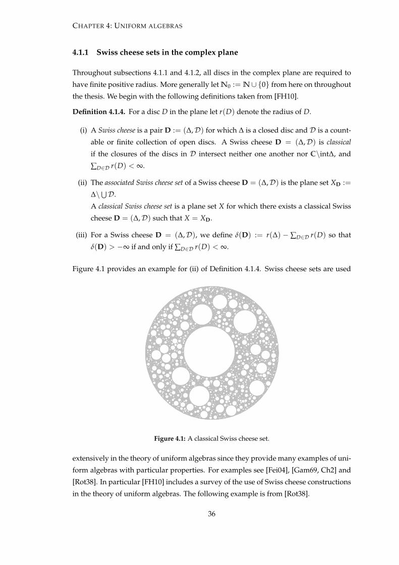
CHAPTER 4: UNIFORM ALGEBRAS
4.1.1 Swiss cheese sets in the complex plane
Throughout subsections 4.1.1 and 4.1.2, all discs in the complex plane are required to
have finite positive radius. More generally let N0 := N∪ {0} from here on throughout
the thesis. We begin with the following definitions taken from [FH10].
Definition 4.1.4. For a disc D in the plane let r(D) denote the radius of D.
(i) A Swiss cheese is a pair D := (∆,D) for which ∆ is a closed disc and D is a count-
able or finite collection of open discs. A Swiss cheese D = (∆,D) is classical
if the closures of the discs in D intersect neither one another nor C\int∆, and
∑D∈D r(D) < ∞.
(ii) The associated Swiss cheese set of a Swiss cheese D = (∆,D) is the plane set XD :=
∆\⋃D.
A classical Swiss cheese set is a plane set X for which there exists a classical Swiss
cheese D = (∆,D) such that X = XD.
(iii) For a Swiss cheese D = (∆,D), we define δ(D) := r(∆) − ∑D∈D r(D) so that
δ(D) > −∞ if and only if ∑D∈D r(D) < ∞.
Figure 4.1 provides an example for (ii) of Definition 4.1.4. Swiss cheese sets are used
Figure 4.1: A classical Swiss cheese set.
extensively in the theory of uniform algebras since they provide many examples of uni-
form algebras with particular properties. For examples see [Fei04], [Gam69, Ch2] and
[Rot38]. In particular [FH10] includes a survey of the use of Swiss cheese constructions
in the theory of uniform algebras. The following example is from [Rot38].
36

CHAPTER 4: UNIFORM ALGEBRAS
Lemma 4.1.5. For X ⊆ C non-empty and compact, let A1 ⊆ A2 ⊆ CC(X) be uniform
algebras with A0 uniformly dense in A1. Suppose we can find a continuous linear functional
ϕ : CC(X)→ C such that ϕ(A0) = {0} and ϕ( f ) = a 6= 0 for some f ∈ A2. Then A1 6= A2.
Proof. Let q ∈ A0. Then
0 < |a|∞ = |ϕ( f )− ϕ(q)|∞ = |ϕ( f − q)|∞ ≤ ‖ f − q‖∞‖ϕ‖op
giving ‖ f − q‖∞ ≥ |a|∞‖ϕ‖−1op > 0 for all q ∈ A0. Hence f can not be uniformly
approximated by elements of A0. More simply, ϕ(A1) = {0} by continuity.
Example 4.1.6. It is possible to have R(X) 6= A(X). Let D0 be a closed disc and let
D = (D0,D) be a classical Swiss cheese with δ(D) > 0 and D infinite. Let (Dn) be
a sequence of open discs such that the map n 7→ Dn is a bijection from N to D. For
n ∈N0 define γn : [0, 1]→ C as the circular path
γn(x) := rn exp(2πix) + an
around the boundary ∂Dn. Now for a rational function q ∈ CC(XD) we note that on C
the finitely many poles of q lie in the open complement of XD and so XD is a subset of
an open subset of C upon which q is analytic. Hence by Cauchy’s theorem, see [Rud87,
p218], we have ϕ(q) = 0 for ϕ : CC(XD)→ C defined by
ϕ( f ) :=∫
γ0
f dz−∞
∑n=1
∫γn
f dz for f ∈ CC(XD).
We now check that ϕ is a bounded linear functional on CC(XD). The following uses the
fundamental estimate. Let f ∈ CC(XD) with ‖ f ‖∞ ≤ 1. Then,
|ϕ( f )|∞ =
∣∣∣∣∣∫
γ0
f (z)dz−∞
∑n=1
∫γn
f (z)dz
∣∣∣∣∣∞
≤∞
∑n=0
∣∣∣∣∫γn
f (z)dz∣∣∣∣∞
≤∞
∑n=0‖ f ‖∞
∫ 1
0|γ′n(x)|∞dx
≤∞
∑n=0
∫ 1
0|rn2πi exp(2πix)|∞dx
=∞
∑n=0
rn2π∫ 1
0dx = 2π
(∞
∑n=0
rn
)< 4πr0
where ∑∞n=0 rn < 2r0 since δ(D) > 0. Now 4πr0 is an upper bound for the series
of absolute terms, hence we have absolute convergence. Since absolute convergence
37

CHAPTER 4: UNIFORM ALGEBRAS
implies convergence we have, for all f ∈ CC(XD),
ϕ( f ) = ϕ
(‖ f ‖∞
‖ f ‖∞f)= ‖ f ‖∞ ϕ
(f‖ f ‖∞
)= ‖ f ‖∞a f ∈ C
for some a f ∈ C. Moreover, our calculation shows that ϕ is bounded with ‖ϕ‖op <
4πr0. The linearity of ϕ follows from the linearity of integrating over a sum of terms
and so ϕ is a continuous linear functional on CC(XD). Next we note that the function
g : z 7→ z on XD given by complex conjugation is an element of CC(XD). Cauchy’s
theorem does not imply that ϕ(g) will be zero since g is not analytic on any non-empty
open subset of C. We have
ϕ(g) =∫
γ0
g(z)dz−∞
∑n=1
∫γn
g(z)dz = 2πi
(r2
0 −∞
∑n=1
r2n
),
since for each n ∈N0∫γn
g(z)dz =∫ 1
0g(γn)γ
′ndx
=∫ 1
0(rn exp(−2πix) + an)rn2πi exp(2πix)dx
= 2πirn
∫ 1
0(rn + an exp(2πix))dx
= 2πirn
(rn
∫ 1
0dx + an
∫ 1
0exp(2πix)dx
)= 2πirn
(rn + an
[1
2πiexp(2πix)
]1
0
)= 2πir2
n.
Furthermore ∑∞n=1 r2
n ≤ (∑∞n=1 rn)2 < r2
0 since ∑∞n=1 rn < r0, by δ(D) > 0, and so
ϕ(g) 6= 0. Therefore by Lemma 4.1.5 we have R(XD) 6= CC(XD) and g 6∈ R(XD).
Certainly this result is immediate in the case where XD has interior since then g will
not be an element of A(XD). However this is one of the occasions where the usefulness
of Swiss cheese set constructions becomes evident since, with some consideration, it is
straightforward to construct a classical Swiss cheese D = (D0,D) with δ(D) > 0 such
that XD has empty interior. Since A(XD) is the uniform algebra of all elements from
CC(XD) that are analytic on the interior of XD, in this case we have A(XD) = CC(XD)
and so by the above R(XD) 6= A(XD) which completes this example.
Let D be a Swiss cheese as specified in Example 4.1.6 such that XD has empty interior.
The following subsection shows that in this case there is actually no need to require D
to be classical in order that R(XD) 6= A(XD).
38
CHAPTER 4: UNIFORM ALGEBRAS
4.1.2 Classicalisation theorem
In this subsection we give a new proof of an existing theorem by J. F. Feinstein and M.
J. Heath, see [FH10]. The theorem states that any Swiss cheese set defined by a Swiss
cheese D with δ(D) > 0 contains a Swiss cheese set as a subset defined by a classical
Swiss cheese D′
with δ(D′) ≥ δ(D). Feinstein and Heath begin their proof by devel-
oping a theory of allocation maps connected to such sets. A partial order on a family
of these allocation maps is then introduced and Zorn’s lemma applied. We take a more
direct approach by using transfinite induction, cardinality and disc assignment func-
tions, where a disc assignment function is a kind of labeled Swiss cheese that defines a
Swiss cheese set. An explicit theory of allocation maps is no longer required although
we are still using them implicitly. In this regard we will discuss the connections with
the original proof of Feinstein and Heath. See [Kel75, p266] and [Dal00, p9] for useful
introductions to ordinals and transfinite induction which has been used in this subsec-
tion. We begin with the following definitions.
Definition 4.1.7. Let O be the set of all open discs and complements of closed discs in
the complex plane.
(i) A disc assignment function d : S → O is a map from a subset S ⊆ N0, with 0 ∈ S,
into O such that Dd := (C\d(0), d(S\{0})) is a Swiss cheese. We allow S\{0} to
be empty since a Swiss cheese D = (∆,D) can have D = ∅.
(ii) For a disc assignment function d : S → O and i ∈ S we let d(i) denote the
closure of d(i) in C, that is d(i) := d(i). A disc assignment function d : S → Ois said to be classical if for all (i, j) ∈ S2 with i 6= j we have d(i) ∩ d(j) = ∅ and
∑n∈S\{0} r(d(n)) < ∞.
(iii) For a disc assignment function d : S → O we let Xd denote the associated Swiss
cheese set of the Swiss cheese Dd.
(iv) A disc assignment function d : S→ O is said to have the Feinstein-Heath condition
when ∑n∈S\{0} r(d(n)) < r(C\d(0)).
(v) Define H as the set of all disc assignment functions with the Feinstein-Heath con-
dition.
For h ∈ H, h : S→ O, define δh := r(C\h(0))−∑n∈S\{0} r(h(n)) > 0.
Here is the Feinstein-Heath Swiss cheese “Classicalisation” theorem as it appears in
[FH10].
39
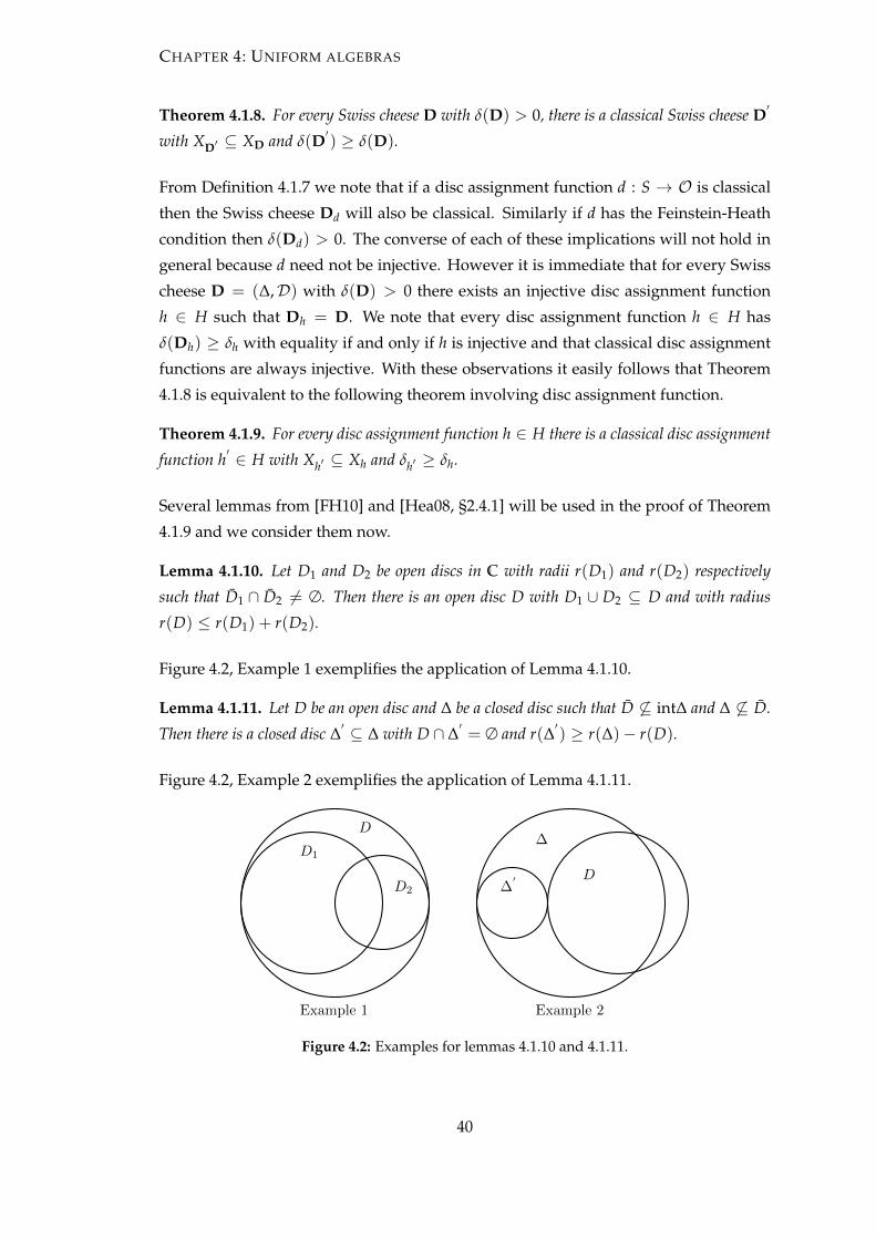
CHAPTER 4: UNIFORM ALGEBRAS
Theorem 4.1.8. For every Swiss cheese D with δ(D) > 0, there is a classical Swiss cheese D′
with XD′ ⊆ XD and δ(D′) ≥ δ(D).
From Definition 4.1.7 we note that if a disc assignment function d : S → O is classical
then the Swiss cheese Dd will also be classical. Similarly if d has the Feinstein-Heath
condition then δ(Dd) > 0. The converse of each of these implications will not hold in
general because d need not be injective. However it is immediate that for every Swiss
cheese D = (∆,D) with δ(D) > 0 there exists an injective disc assignment function
h ∈ H such that Dh = D. We note that every disc assignment function h ∈ H has
δ(Dh) ≥ δh with equality if and only if h is injective and that classical disc assignment
functions are always injective. With these observations it easily follows that Theorem
4.1.8 is equivalent to the following theorem involving disc assignment function.
Theorem 4.1.9. For every disc assignment function h ∈ H there is a classical disc assignment
function h′ ∈ H with Xh′ ⊆ Xh and δh′ ≥ δh.
Several lemmas from [FH10] and [Hea08, §2.4.1] will be used in the proof of Theorem
4.1.9 and we consider them now.
Lemma 4.1.10. Let D1 and D2 be open discs in C with radii r(D1) and r(D2) respectively
such that D1 ∩ D2 6= ∅. Then there is an open disc D with D1 ∪ D2 ⊆ D and with radius
r(D) ≤ r(D1) + r(D2).
Figure 4.2, Example 1 exemplifies the application of Lemma 4.1.10.
Lemma 4.1.11. Let D be an open disc and ∆ be a closed disc such that D 6⊆ int∆ and ∆ 6⊆ D.
Then there is a closed disc ∆′ ⊆ ∆ with D ∩ ∆
′= ∅ and r(∆
′) ≥ r(∆)− r(D).
Figure 4.2, Example 2 exemplifies the application of Lemma 4.1.11.
D1
D2
D
Example 1
∆
∆′ D
Example 2
Figure 4.2: Examples for lemmas 4.1.10 and 4.1.11.
40

CHAPTER 4: UNIFORM ALGEBRAS
Lemma 4.1.12. Let F be a non-empty, nested collection of open discs in C, such that we have
sup{r(E) : E ∈ F} < ∞. Then⋃F is an open disc D. Further, for F ordered by inclusion,
r(D) = limE∈F r(E) = supE∈F r(E).
Lemma 4.1.13. Let F be a non-empty, nested collection of closed discs in C, such that we have
inf{r(E) : E ∈ F} > 0. Then⋂F is a closed disc ∆. Further, for F ordered by reverse
inclusion, r(∆) = limE∈F r(E) = infE∈F r(E).
Proof of Theorem 4.1.9. At the heart of the proof of Theorem 4.1.9 is a completely defined
map f : H → H which we now define case by case.
Definition 4.1.14. Let f : H → H be the self map with the following construction.
Case 1: If h ∈ H is a classical disc assignment function then define f (h) := h.
Case 2: If h ∈ H is not classical then for h : S→ O let
Ih := {(i, j) ∈ S2 : h(i) ∩ h(j) 6= ∅, i 6= j}.
We then have lexicographic ordering on Ih given by
(i, j) . (i′, j′) if and only if i < i
′or (i = i
′and j ≤ j
′).
Since this is a well-ordering on Ih, let (n, m) be the minimum element of Ih and hence
note that m 6= 0 since m > n. We proceed toward defining f (h) : S′ → O.
Define S′
:= S\{m} and for i ∈ S′\{n} we define f (h)(i) := h(i).
It remains for the definition of f (h)(n) to be given and to this end we have the follow-
ing two cases.
Case 2.1: n 6= 0. In this case, by Definition 4.1.7, we note that both h(m) and h(n)
are open discs. Associating h(m) and h(n) with D1 and D2 of Lemma 4.1.10 we de-
fine f (h)(n) to be the open disc satisfying the properties of D of the lemma. Note in
particular that,
h(m) ∪ h(n) ⊆ f (h)(n) with n < m. (4.1.1)
Case 2.2: n = 0. In this case, by Definition 4.1.7, we note that h(m) is an open disc and
h(0) is the complement of a closed disc. Associate h(m) with D from Lemma 4.1.11 and
put ∆ := C\h(0). Since (0, m) ∈ Ih we have h(0) ∩ h(m) 6= ∅ and so h(m) 6⊆ int∆,
noting int∆ = C\h(0). Further, since h ∈ H we have r(h(m)) < r(∆) and so ∆ 6⊆ h(m).
Therefore the conditions of Lemma 4.1.11 are satisfied for h(m) and ∆. Hence we define
f (h)(0) to be the complement of the closed disc satisfying the properties of ∆′of Lemma
4.1.11. Note in particular that,
h(m) ∪ h(0) ⊆ f (h)(0) with 0 < m. (4.1.2)
41

CHAPTER 4: UNIFORM ALGEBRAS
For this definition of the map f we have yet to show that f maps into H. We now show
this together with certain other useful properties of f .
Lemma 4.1.15. Let h ∈ H, then the following hold:
(i) f (h) ∈ H with δ f (h) ≥ δh;
(ii) For (h : S → O) 7→ ( f (h) : S′ → O) we have S
′ ⊆ S with equality if and only if h is
classical. Otherwise S′= S\{m} for some m ∈ S\{0};
(iii) X f (h) ⊆ Xh;
(iv) For all i ∈ S′, h(i) ⊆ f (h)(i).
Proof. We need only check (i) and (iii) for cases 2.1 and 2.2 of the definition of f , as
everything else is immediate. Let h ∈ H.
(i) It is clear that f (h) is a disc assignment function. It remains to check that δ f (h) ≥ δh.
For Case 2.1 we have, by Lemma 4.1.10,
δh = r(C\h(0))− (r(h(m)) + r(h(n)))− ∑i∈S\{0,m,n}
r(h(i))
≤ r(C\h(0))− r( f (h)(n))− ∑i∈S\{0,m,n}
r(h(i)) = δ f (h).
For Case 2.2 we have, by Lemma 4.1.11,
δh = r(C\h(0))− r(h(m))− ∑i∈S\{0,m}
r(h(i))
≤ r(C\ f (h)(0))− ∑i∈S\{0,m}
r(h(i)) = δ f (h).
(iii) Since Xh = C\⋃i∈S h(i) we require⋃
i∈S h(i) ⊆ ⋃i∈S′ f (h)(i).
For Case 2.1 we have by Lemma 4.1.10 that h(m) ∪ h(n) ⊆ f (h)(n), as shown at (4.1.1),
giving⋃
i∈S h(i) ⊆ ⋃i∈S′ f (h)(i).
For Case 2.2 put ∆ := C\h(0) and ∆′
:= C\ f (h)(0). We have by Lemma 4.1.11 that
∆′ ⊆ ∆ and h(m) ∩ ∆
′= ∅. Hence h(0) ∪ h(m) ⊆ f (h)(0), as shown at (4.1.2), and so⋃
i∈S h(i) ⊆ ⋃i∈S′ f (h)(i) as required.
We will use f : H → H to construct an ordinal sequence of disc assignment functions
and then apply a cardinality argument to show that this ordinal sequence must stabilise
at a classical disc assignment function. We construct the ordinal sequence so that it has
the right properties.
Definition 4.1.16. Let h ∈ H.
42
CHAPTER 4: UNIFORM ALGEBRAS
(a) Define h0 : S0 → D by h0 := h.
Now let α > 0 be an ordinal for which we have defined hβ ∈ H for all β < α.
(b) If α is a successor ordinal then define hα : Sα → O by hα := f (hα−1).
(c) If α is a limit ordinal then define hα : Sα → O as follows.
Set Sα :=⋂
β<α
Sβ. Then for n ∈ Sα define hα(n) :=⋃
β<α
hβ(n).
Suppose that for every ordinal α for which Definition 4.1.16 can be applied we have
hα ∈ H. Then Definition 4.1.16 can be applied for every ordinal α by transfinite induc-
tion and therefore defines an ordinal sequence of disc assignment function. We will use
transfinite induction to prove Lemma 4.1.17 below which asserts that hα is an element
of H as well as other useful properties of hα.
Lemma 4.1.17. Let α be an ordinal number and let h ∈ H. Then the following hold:
(α,1) hα ∈ H with δhα ≥ δh;
(α,1.1) 0 ∈ Sα;
(α,1.2) hα(0) is the complement of a closed disc and
hα(n) is an open disc for all n ∈ Sα\{0};
(α,1.3) ∑n∈Sα\{0} r(hα(n)) ≤ r(C\hα(0))− δh;
(α,2) For all β ≤ α we have Sα ⊆ Sβ;
(α,3) For all β ≤ α we have Xhα ⊆ Xhβ ;
(α,4) For all n ∈ Sα, {hβ(n) : β ≤ α} is a nested increasing family of open sets.
Proof. We will use transfinite induction.
For α an ordinal number let P(α) be the proposition, Lemma 4.1.17 holds at α.
The base case P(0) is immediate and our inductive hypothesis is that for all β < α, P(β)
holds.
Now for α a successor ordinal we have hα = f (hα−1) and so P(α) is immediate by the
inductive hypothesis and Lemma 4.1.15. Now suppose α is a limit ordinal. We have
Sα :=⋂
β<α Sβ giving, for all β ≤ α, Sα ⊆ Sβ. Hence (α,2) holds. Also for all β < α we
have 0 ∈ Sβ by (β,1.1). So 0 ∈ Sα showing that (α,1.1) holds. To show (α,1.2) we will
use lemmas 4.1.12 and 4.1.13.
43

CHAPTER 4: UNIFORM ALGEBRAS
(i) Now for all n ∈ Sα\{0}, {hβ(n) : β < α} is a nested increasing family of open
discs by (β,1.2) and (β,4).
(ii) Further, {C\hβ(0) : β < α} is a nested decreasing family of closed discs by (β,1.2)
and (β,4).
(iii) Now for n ∈ Sα\{0} and β < α we have
r(hβ(n)) ≤ ∑m∈Sβ\{0} r(hβ(m)) = r(C\hβ(0)) − δhβ ≤ r(C\h(0)) − δh, by (β,1)
and (ii). Hence sup{r(hβ(n)) : β < α} ≤ r(C\h(0))− δh. So by (i) and Lemma
4.1.12 we have for n ∈ Sα\{0} that
hα(n) :=⋃
β<α
hβ(n)
is an open disc with,
r(hα(n)) = supβ<α
r(hβ(n)) ≤ r(C\h(0))− δh.
(iv) Now for β < α we have r(C\hβ(0)) ≥ δh by (β,1.3).
Hence inf{r(C\hβ(0)) : β < α} ≥ δh. So by De Morgan, (ii) and Lemma 4.1.13 we
have
C\hα(0) := C\⋃
β<α
hβ(0) =⋂
β<α
C\hβ(0)
is a closed disc with,
r(C\hα(0)) = infβ<α
r(C\hβ(0)) ≥ δh.
Hence hα(0) is the complement of a closed disc and so (α,1.2) holds.
We now show that (α,4) holds. By (β,4) we have, for all n ∈ Sα, {hβ(n) : β < α} is
a nested increasing family of open sets. We also have hα(n) =⋃
β<α hβ(n) so, for all
β ≤ α, hβ(n) ⊆ hα(n) and hα(n) is an open set since (α,1.2) holds. Hence (α,4) holds.
We will now show that (α,1.3) holds. We first prove that, for all λ < α, we have
∑m∈Sα\{0}
r(hα(m)) ≤ r(C\hλ(0))− δh. (4.1.3)
Let λ < α, and suppose, towards a contradiction, that
∑m∈Sα\{0}
r(hα(m)) > r(C\hλ(0))− δh, (4.1.4)
noting that the right hand side of (4.1.4) is non-negative by (λ,1.3).
Set
ε :=12
(∑
m∈Sα\{0}r(hα(m))− (r(C\hλ(0))− δh)
)> 0.
44

CHAPTER 4: UNIFORM ALGEBRAS
Then there exists n ∈ Sα\{0} such that for Sα|n1 := {m ∈ Sα\{0} : m ≤ n} we have
∑m∈Sα|n1
r(hα(m)) > r(C\hλ(0))− δh + ε > 0. (4.1.5)
Further for each m ∈ Sα|n1 we have, by (iii), r(hα(m)) = supβ<α r(hβ(m)). Hence for
each m ∈ Sα|n1 there exists βm < α such that r(hβm(m)) ≥ r(hα(m)) − 12k ε, for k :=
|Sα|n1 |, k 6= 0 by (4.1.5). Let λ′
:= max{βm : m ∈ Sα|n1} < α and note that this is a
maximum over a finite set of elements since Sα|n1 ⊆ N is finite. Now for any γ with
max{λ, λ′} ≤ γ < α we have,
∑m∈Sγ\{0}
r(hγ(m)) ≥ ∑m∈Sα\{0}
r(hγ(m)) (since Sα ⊆ Sγ)
≥ ∑m∈Sα|n1
r(hγ(m))
≥ ∑m∈Sα|n1
r(hβm(m)) (by (γ,4))
≥ ∑m∈Sα|n1
(r(hα(m))− ε
2k) (by the above)
> r(C\hλ(0))− δh + ε− kε
2k(by (4.1.5) and k := |Sα|n1 |)
> r(C\hλ(0))− δh
≥ r(C\hγ(0))− δh (by (ii)).
This contradicts (γ,1.3). Hence we have shown that, for all λ < α, (4.1.3) holds.
Now by (iv) we have r(C\hα(0)) = infλ<α r(C\hλ(0)).
Hence we have ∑m∈Sα\{0} r(hα(m)) ≤ r(C\hα(0))− δh and so (α,1.3) holds.
We now show that (α,3) holds. We will show that for all ordinals β < α,⋃i∈Sβ
hβ(i) ⊆ ⋃i∈Sαhα(i). Let β < α and z ∈ ⋃i∈Sβ
hβ(i). Define,
m := min{i ∈N0 : there exists λ < α with i ∈ Sλ and z ∈ hλ(i)}.
By the definition of m there exists ζ < α with m ∈ Sζ and z ∈ hζ(m). We claim that the
set {λ < α : m 6∈ Sλ} is empty. To prove this suppose towards a contradiction that we
can define,
λ′
:= min{λ < α : m 6∈ Sλ}.
Then λ′> 0 since, by (ζ,2), Sζ ⊆ S0 with m ∈ Sζ . If λ
′is a limit ordinal then m 6∈ Sλ
′ =⋂γ<λ
′ Sγ giving m 6∈ Sγ, for some γ < λ′, and this contradicts the definition of λ
′. If
λ′
is a successor ordinal then hλ′= f (hλ
′−1) with m ∈ Sλ′−1 by the definition of λ
′. By
m 6∈ Sλ′ and Definition 4.1.14 of f : H → H, hλ
′−1 is not classical. Therefore by (4.1.1)
and (4.1.2) of Definition 4.1.14 there is n ∈ Sλ′ with n < m and hλ
′−1(m) ⊆ hλ′(n).
Further for all λ with λ′ ≤ λ < α we have m 6∈ Sλ since m 6∈ Sλ
′ and, by (λ,2), Sλ ⊆ Sλ′ .
45

CHAPTER 4: UNIFORM ALGEBRAS
Hence we have ζ < λ′. Now, by (λ
′ − 1, 4), {hγ(m) : γ ≤ λ′ − 1} is a nested increasing
family of sets giving z ∈ hζ(m) ⊆ hλ′−1(m) ⊆ hλ
′(n) with n ∈ Sλ
′ . This contradicts the
definition of m since n < m. Hence we have shown that {λ < α : m 6∈ Sλ} is empty
giving m ∈ Sα =⋂
λ<α Sλ. Therefore, by Definition 4.1.16 and the definition of ζ, we
have z ∈ hζ(m) ⊆ ⋃λ<α hλ(m) = hα(m) ⊆ ⋃
i∈Sαhα(i) as required. Hence (α,3) holds.
Therefore we have shown, by the principal of transfinite induction, that P(α) holds and
this concludes the proof of Lemma 4.1.17.
Recall that our aim is to prove that for every h ∈ H there is a classical disc assignment
function h′ ∈ H with Xh′ ⊆ Xh and δh′ ≥ δh. We have the following closing argument
using cardinality. By (α,2) of Lemma 4.1.17 we obtain a nested ordinal sequence of
domains (Sα),
N0 ⊇ S ⊇ S1 ⊇ S2 ⊇ · · · ⊇ Sω ⊇ Sω+1 ⊇ · · · ⊇ {0}.Now setting Sc
α := N0\Sα gives a nested ordinal sequence (Scα),
∅ ⊆ Sc ⊆ Sc1 ⊆ Sc
2 ⊆ · · · ⊆ Scω ⊆ Sc
ω+1 ⊆ · · · ⊆N.
Lemma 4.1.18. For the disc assignment function hβ we have,
hβ is classical if and only if (Sα) has stabilised at β, i.e. Sβ+1 = Sβ.
Proof. The proof follows directly from (ii) of Lemma 4.1.15.
Now let ω1 be the first uncountable ordinal. Suppose towards a contradiction that,
for all β < ω1, (Sα) has not stabilised at β. Then for each β < ω1 there exists some
nβ+1 ∈ N such that nβ+1 ∈ Scβ+1 but nβ+1 6∈ Sc
α for all α ≤ β. Hence since there are
uncountably many β < ω1 we have Scω1
uncountable with Scω1⊆ N, a contradiction.
Therefore there exists β < ω1 such that (Sα) has stabilised at β and so, by Lemma 4.1.18,
hβ is classical. Now by (β,1) of Lemma 4.1.17 we have hβ ∈ H with δhβ ≥ δh and by
(β,3) we have Xhβ ⊆ Xh. In particular this completes the proof of Theorem 4.1.9 and
the Feinstein-Heath Swiss cheese “Classicalisation” theorem.
The proof of Theorem 4.1.8 as presented above proceeded without reference to a theory
of allocation maps. In the original proof of Feinstein and Heath, [FH10], allocation
maps play a central role. We will recover a key allocation map from the original proof
using the map f : H → H of Definition 4.1.14. Here is the definition of an allocation
map as it appears in [FH10].
Definition 4.1.19. Let D = (∆,D) be a Swiss cheese. We define
D = D ∪ {C\∆}.
Now let E = (E, E) be a second Swiss cheese, and let f : D → E. We define G( f ) =
f−1(C\E) ∩D. We say that f is an allocation map if the following hold:
46

CHAPTER 4: UNIFORM ALGEBRAS
(A1) for each U ∈ D, U ⊆ f (U);
(A2)
∑D∈G( f )
r(D) ≥ r(∆)− r(E);
(A3) for each E ∈ E ,
∑D∈ f−1(E)
r(D) ≥ r(E).
Let D be the Swiss cheese of Theorem 4.1.8 and let S(D) be the family of allocation
maps defined on D. In [FH10] a partial order is applied to S(D) and subsequently a
maximal element fmax is obtained using Zorn’s lemma. The connection between al-
location maps and Swiss cheeses is then exploited. Towards a contradiction the non-
existence of the desired classical Swiss cheese D′
of Theorem 4.1.8 is assumed. This
assumption implies the existence of an allocation map f ′ ∈ S(D) that is higher in the
partial order applied to S(D) than fmax, a contradiction. The result follows. It is at the
last stage of the original proof where a connection to the new version can be found. In
the construction of Feinstein and Heath the allocation map f ′ factorizes as f ′ = g ◦ fmax
where g is also an allocation map. Let E = (E, E) be a non-classical Swiss cheese with
δ(E) > 0. Using the same method of construction that Feinstein and Heath use for
g, an allocation map gE defined on E can be obtained without contradiction. Clearly
E 6= fmax(D). We will obtain gE using the map f : H → H of Definition 4.1.14. Let
h ∈ H, h : S→ O, be an injective disc assignment function such that Dh = E and recall
from Definition 4.1.14 that f (h) : S′ → O has S
′= S\{m}where (n, m) is the minimum
element of Ih. Set E′ := D f (h). By Definitions 4.1.7 and 4.1.19 we have
E = Dh = h(S) and E′ = D f (h) = f (h)(S′).
Now define a map ι : E→ S′
by,
for U ∈ E, ι(U) :=
h−1(U) if h−1(U) 6= m
n if h−1(U) = m,
and note that this is well defined since h is injective. The commutative diagram in Fig-
EgE //
�
E′
S′
f (h)
??
Figure 4.3: gE = f (h) ◦ ι.
ure 4.3 show how gE is obtained using f : H → H. The construction of f in Definition
47

CHAPTER 4: UNIFORM ALGEBRAS
4.1.14 was developed from the construction that Feinstein and Heath used for g. The
method of combining discs in Lemma 4.1.10 also appears in [Zha93].
Remark 4.1.20. Concerning classicalisation.
(i) Interestingly, as Heath points out in [FH10], every classical Swiss cheese set in
C with empty interior is homeomorphic to the Sierpinski carpet. Hence up to
homeomorphism there is only 1 Swiss cheese set of this type. In particular if
XD is a Swiss cheese contained in C with empty interior then either one of the
conditions XD is classical or δ(D) > 0 is enough for R(XD) 6= A(XD).
(ii) I also anticipate the possibility of an analog of Theorem 4.1.9 on the sphere. Let
S ⊆ R3 be a sphere of finite positive radius rs and center c ∈ R3. For a, b ∈ S let
ds(a, b) := rs∠acb be the length of the geodesic path in S from a to b. Now ds is a
metric with respect to which we will define open and closed S-discs contained in
S. With analogy to Definition 4.1.4 let Ds := (∆,D) be a Swiss cheese on S. Then
either ∆ = S or D′s := (S,D ∪ {S\∆}) is a Swiss cheese on S, since S\∆ is an open
S-disc, for which XD′s= XDs in S. Further we have
δ(Ds) := r(∆)− ∑D∈D
r(D) = πrs − r(S\∆)− ∑D∈D
r(D) = δ(D′s)
and so for our choice of metric on S we note that δ is independent of whether we
use Ds or D′s. Hence the situation for the sphere is a little simpler than that for the
plane since we can allow all Swiss cheeses on the sphere to have the form Ds :=
(S,D) and avoid the need to handle a special closed S-disc ∆. Therefore on the
sphere analogs of lemmas 4.1.11 and 4.1.13 are not required. We will not establish
here whether the condition δ(Ds) > 0 is sufficient for the analog of Theorem 4.1.9
on S to hold since the next step in generalising this theorem should be to establish
the class of all metric spaces for which a general version of the theorem holds.
However the sphere is of particular interest in the context of uniform algebras
since, less one point, the sphere is homeomorphic to the plane allowing many
examples of uniform algebras to be defined on subsets of the sphere.
4.2 Non-complex analogs of uniform algebras
The most obvious non-complex analog of Definition 4.1.1 is obtained by simply replac-
ing the complex numbers in the definition by some other complete valued field F. In
this case, whilst CF(X) will be complete and contain the constants, we need to take
care concerning the topology on X when F is non-Archimedean, e.g. CQp([0, 1]) only
contains the constant.
48

CHAPTER 4: UNIFORM ALGEBRAS
Theorem 4.2.1. Let F be a complete non-Archimedean valued field and let CF(X) be the unital
Banach F-algebra of all continuous F-valued functions defined on a compact, Hausdorff space
X. Then CF(X) separates the points of X if and only if X is totally disconnected.
Before giving a proof of Theorem 4.2.1 we have the following version of Urysohn’s
lemma which will certainly already be known in some form because of its simplicity.
Lemma 4.2.2. Let X be a totally disconnected, compact, Hausdorff space with finite subset
{x, y1, y2, y3, · · · , yn} ⊆ X, x 6= yi for all i ∈ {1, · · · , n} where n ∈ N. Let L be any non-
empty topological space and a, b ∈ L. Then there exists a continuous map h : X −→ L such
that h(x) = a and h(y1) = h(y2) = h(y3) = · · · = h(yn) = b.
Proof. Since X is a Hausdorff space, for each i ∈ {1, · · · , n} there are disjoint open
subsets Ui and Vi of X with x ∈ Ui and yi ∈ Vi. Hence U :=⋂
i∈{1,··· ,n}Ui is an open
subset of X with x ∈ U and U ∩Vi = ∅ for all i ∈ {1, · · · , n}. Now since X is a totally
disconnected, compact, Hausdorff space, x has a neighborhood base of clopen sets, see
[Wil04, Theorem 29.7] noting that X is locally compact by Theorem 2.1.22. Hence there
is a clopen subset W of X with x ∈ W ⊆ U. The function h : X −→ L given by
h(W) := {a} and h(X\W) := {b} is continuous as required.
We now give the proof of Theorem 4.2.1.
Proof. With reference to Lemma 4.2.2 it remains to show that CF(X) separates the points
of X only if X is totally disconnected. Let X be a compact, Hausdorff space such that
CF(X) separates the points of X. Let U be a non-empty connected subset of X and
let f ∈ CF(X). We note that f (U) is a connected subset of F since f is continuous.
Now, since F is non-Archimedean it is totally disconnected i.e. its connected subsets
are singletons. Hence f (U) is a singleton and so f is constant on U. Therefore, since
CF(X) separates the points of X, U is a singleton and X is totally disconnected.
We next consider the constraints on CF(X) revealed by generalisations of the Stone-
Weierstrass theorem. In the real case the Stone-Weierstrass theorem for CR(X) says
that for every compact Hausdorff space X, CR(X) is without a proper subalgebra that
is uniformly closed, contains the real numbers and separates the points of X. A proof
can be found in [KL92, p50]. The non-Archimedean case is given by a theorem of
Kaplansky, see [Ber90, p157] or [Kap50].
Theorem 4.2.3. Let F be a complete non-Archimedean valued field, let X be a totally dis-
connected compact Hausdorff space, and let A be a F-subalgebra of CF(X) which satisfies the
following conditions:
49

CHAPTER 4: UNIFORM ALGEBRAS
(i) the elements of A separate the points of X;
(ii) for each x ∈ X there exists f ∈ A with f (x) 6= 0.
Then A is everywhere dense in CF(X).
Note that, in Theorem 4.2.3, A being a F-subalgebra of CF(X) means that A is a sub-
algebra of CF(X) and a vector space over F. If we take A to be unital then condition
(ii) in Theorem 4.2.3 is automatically satisfied and the theorem is analogous to the real
version of the Stone-Weierstrass theorem. In subsection 4.2.1 we will see that real func-
tion algebras are a useful example when considering non-complex analogs of uniform
algebras with qualifying subalgebras.
4.2.1 Real function algebras
Real function algebras were introduced by Kulkarni and Limaye in a paper from 1981,
see [KL81]. For a thorough text on the theory see [KL92]. The following definition is a
little more general than what we need in this subsection.
Definition 4.2.4. Let X be a topological space and let τ : X → X be a homeomorphism.
(i) We will call τ a topological involution on X if τ ◦ τ = id on X.
(ii) We will call τ a topological element of finite order on X if τ has finite order but with
ord(τ) > 2.
Let F and L be complete valued fields such that L is a finite extension of F as a valued
field and let g ∈ Gal(L/F). Let A either be an F-algebra or an L-algebra for which
σ : A→ A is a map satisfying ord(σ) = ord(g) and for all a, b ∈ A and scalars α:
σ(a + b) = σ(a) + σ(b);
σ(ab) = σ(b)σ(a);
σ(αa) = g(α)σ(a).
(iii) We will call σ a algebraic involution on A if σ ◦ σ = id on A.
(iv) We will call σ a algebraic element of finite order on A if σ has ord(σ) > 2.
Note, in Definition 4.2.4 the requirement that τ be a homeomorphism is satisfied if τ is
continuous.
50

CHAPTER 4: UNIFORM ALGEBRAS
Definition 4.2.5. Let X be a compact Hausdorff space and τ a topological involution
on X. A real function algebra on (X, τ) is a real subalgebra A of
C(X, τ) := { f ∈ CC(X) : f (τ(x)) = f (x) for all x ∈ X}
that is complete with respect to the sup norm, contains the real numbers and separates
the points of X.
Remark 4.2.6. Concerning real function algebras.
(i) Later, Theorem 5.2.1 will confirm that C(X, τ) in Definition 4.2.5 is itself always a
real function algebra on (X, τ) and in some sense it is to real function algebras as
CC(X) is to complex uniform algebras.
(ii) Let X be a compact Hausdorff space and Y a closed non-empty subset of X. Then
CY := { f ∈ CC(X) : f (Y) ⊆ R} is a commutative real Banach algebra. As
pointed out in [KL92, p2], every such CY can be transformed into a real function
algebra but the converse of this is false. Hence Definition 4.2.5 is a more general
object.
(iii) With reference to Definition 4.2.5 we have C(X, τ) = { f ∈ CC(X) : σ( f ) = f }where σ( f ) := f ◦ τ. Moreover σ is an algebraic involution on CC(X) and every
algebraic involution on CC(X) arises from a topological involution on X in this
way, see [KL92, p29] for a proof.
The following example is a useful standard.
Example 4.2.7. Recall from Example 4.1.3 the disc algebra A(∆) on the closed unit disc
and let τ : ∆ −→ ∆ be the map τ(z) := z given by complex conjugation, which we note
is a Galois automorphism on C. Now let
B(∆) := A(∆) ∩ C(∆, τ).
We see that B(∆) is complete since both A(∆) and C(∆, τ) are, and similarly B(∆)
contains the real numbers. Further by the definition of C(∆, τ) and the fact that A(∆) =
P(∆) we have that B(∆) is the R-algebra of all uniform limits of polynomials on ∆ with
real coefficients. Hence B(∆) separates the points of ∆ since it contains the function
f (z) := z. However whilst τ is in C(∆, τ) it is not an element of A(∆). Therefore B(∆)
is a real function algebra on (∆, τ) and a proper subalgebra of C(∆, τ). It is referred to
as the real disc algebra.
Finally for each compact Hausdorff space X, CC(X) can be put into the form of a real
function algebra as the following example shows. In particular C can be expressed as
a real function algebra on a two point set.
51

CHAPTER 4: UNIFORM ALGEBRAS
Example 4.2.8. Let X be a compact Hausdorff space, let Y := {i,−i} ⊆ C have the
trivial topology and give X×Y the product topology. We note that the subspace given
by Xi := {(x, y) ∈ X × Y : y = i} is homeomorphic to X and similarly so is X−i.
Define a topological involution τ : X × Y → X × Y by (x, y) 7→ (x, y). Then CC(Xi) is
isometrically isomorphic to C(X×Y, τ) by way of the mapping f 7→ h f where
h f (z) :=
f (z) if z ∈ Xi
f (τ(z)) if z ∈ X−i
, for f ∈ CC(Xi),
so that for z ∈ Xi we have
h f (τ(z)) = f (τ(τ(z))) = f (z) = h f (z)
and for z ∈ X−i
h f (τ(z)) = f (τ(z)) = ¯f (τ(z)) = h f (z)
showing that h f ∈ C(X × Y, τ). The inverse mapping from C(X × Y, τ) to CC(Xi) is
given by the restriction map h 7→ h|Xi . One might suspect that such a mapping exists
for every C(Z, τ) by restricting its elements to a compact subspace of equivalence class
representatives for the forward orbits of τ. But this is not the case in general since
there can be z ∈ Z with ord(τ, z) = 1 forcing all of the functions to be real valued at z
preventing the representation of the complex constants in C(Z, τ).
52
CHAPTER 5
Commutative generalisation over
complete valued fields
If J is a maximal ideal of a commutative unital complex Banach algebra A then J has
codimension one since A/J with the quotient norm is isometrically isomorphic to the
complex numbers. This follows from the Gelfand-Mazur theorem noting that A/J with
the quotient norm is unital since J is closed as a subset of A and J is different to A, see
Lemma 6.1.7 and [Sto71, p16].
In contrast, for a complete non-Archimedean field F, if I is a maximal ideal of a com-
mutative unital Banach F-algebra then I may have large finite or infinite codimension,
note Corollary 2.2.4. Hence, with Gelfand transform theory in mind, it makes sense
to consider non-Archimedean analogs of uniform algebras in the form suggested by
real function algebras where the functions take values in a complete extension of the
underlying field of scalars. Moreover when there is a lattice of intermediate fields then
these fields provide a way for a lattice of extensions of the algebra to occur. See [Ber90,
Ch1] and [Esc03, Ch15] for one form of the Gelfand transform in the non-Archimedean
setting. This chapter introduces the main definitions of interest in the thesis. We will
generalise the definitions made by Kulkarni and Limaye to all complete valued fields,
show that the algebras obtained all qualify as generalisations of uniform algebras and
that restricting attention to the Archimedean setting recovers the complex uniform al-
gebras and real function algebras. Non-Archimedean examples and residue algebras
are also introduced.
5.1 Main definitions
The following definition gives the requirements for those commutative algebras that
are to be considered as generalisations of uniform algebras.
53

CHAPTER 5: COMMUTATIVE GENERALISATION OVER COMPLETE VALUED FIELDS
Definition 5.1.1. Let F and L be complete valued fields such that L is an extension of
F as a valued field. Let X be a compact Hausdorff space and let CL(X) be the unital
Banach L-algebra of all continuous L-valued functions on X with pointwise operations
and the sup norm. If a subset A of CL(X) satisfies:
(i) A is an F-algebra under pointwise operations;
(ii) A is complete with respect to ‖ · ‖∞;
(iii) F ⊆ A;
(iv) A separates the points of X,
then we will call A an L/F uniform algebra or just a uniform algebra when convenient.
In the language of Definition 5.1.1, an L/F uniform algebra is a Banach F-algebra of
L-valued functions, also every L/L uniform algebra is an L/F uniform algebra. We now
generalise, in two parts, Kulkarni and Limaye’s definition of a real function algebra.
Definition 5.1.2. Let F and L be complete valued fields such that L is a finite extension
of F as a valued field. Let X be a compact Hausdorff space and totally disconnected if
F is non-Archimedean. Define C(X, τ, g) ⊆ CL(X) as the subset of elements f ∈ CL(X)
for which the diagram in Figure 5.1 commutes.
Xf
//
τ
��
L
g
��
(i) g ∈ Gal(L/F);
Where: (ii) τ : X → X with ord(τ)|ord(g);
Xf
// L (iii) g and τ are continuous.
Figure 5.1: Commutative diagram for f ∈ C(X, τ, g).
We will call C(X, τ, g) := { f ∈ CL(X) : f (τ(x)) = g( f (x)) for all x ∈ X} the basic L/Lg
function algebra on (X, τ, g) or just a basic function algebra when convenient.
Definition 5.1.3. Let F and L be complete valued fields such that L is a finite extension
of F as a valued field. Let (X, τ, g) conform to the conditions of Definition 5.1.2 and let
A be a subset of the basic L/Lg function algebra on (X, τ, g). If A is also an L/Lg uniform
algebra then we will call A an L/Lg function algebra on (X, τ, g).
Remark 5.1.4. In definitions 5.1.2 and 5.1.3 the valued field Lg is complete by Remark
2.2.2. The continuity of g in Definition 5.1.2 is only an observation since g is an isometry
on L by Remark 2.2.6. In fact g also acts as an isometric automorphism on C(X, τ, g).
54
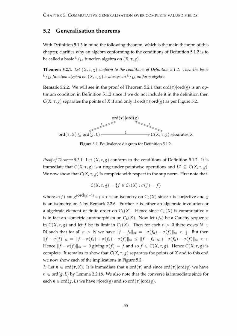
CHAPTER 5: COMMUTATIVE GENERALISATION OVER COMPLETE VALUED FIELDS
5.2 Generalisation theorems
With Definition 5.1.3 in mind the following theorem, which is the main theorem of this
chapter, clarifies why an algebra conforming to the conditions of Definition 5.1.2 is to
be called a basic L/Lg function algebra on (X, τ, g).
Theorem 5.2.1. Let (X, τ, g) conform to the conditions of Definition 5.1.2. Then the basicL/Lg function algebra on (X, τ, g) is always an L/Lg uniform algebra.
Remark 5.2.2. We will see in the proof of Theorem 5.2.1 that ord(τ)|ord(g) is an op-
timum condition in Definition 5.1.2 since if we do not include it in the definition then
C(X, τ, g) separates the points of X if and only if ord(τ)|ord(g) as per Figure 5.2.
ord(τ)|ord(g)1
qyord(τ, X) ⊆ ord(g, L) 2 +3 C(X, τ, g) separates X
3em
Figure 5.2: Equivalence diagram for Definition 5.1.2.
Proof of Theorem 5.2.1. Let (X, τ, g) conform to the conditions of Definition 5.1.2. It is
immediate that C(X, τ, g) is a ring under pointwise operations and Lg ⊆ C(X, τ, g).
We now show that C(X, τ, g) is complete with respect to the sup norm. First note that
C(X, τ, g) = { f ∈ CL(X) : σ( f ) = f }
where σ( f ) := g(ord(g)−1) ◦ f ◦ τ is an isometry on CL(X) since τ is surjective and g
is an isometry on L by Remark 2.2.6. Further σ is either an algebraic involution or
a algebraic element of finite order on CL(X). Hence since CL(X) is commutative σ
is in fact an isometric automorphism on CL(X). Now let ( fn) be a Cauchy sequence
in C(X, τ, g) and let f be its limit in CL(X). Then for each ε > 0 there exists N ∈N such that for all n > N we have ‖ f − fn‖∞ = ‖σ( fn) − σ( f )‖∞ < ε
2 . But then
‖ f − σ( f )‖∞ = ‖ f − σ( fn) + σ( fn) − σ( f )‖∞ ≤ ‖ f − fn‖∞ + ‖σ( fn) − σ( f )‖∞ < ε.
Hence ‖ f − σ( f )‖∞ = 0 giving σ( f ) = f and so f ∈ C(X, τ, g). Hence C(X, τ, g) is
complete. It remains to show that C(X, τ, g) separates the points of X and to this end
we now show each of the implications in Figure 5.2.
1: Let n ∈ ord(τ, X). It is immediate that n|ord(τ) and since ord(τ)|ord(g) we have
n ∈ ord(g, L) by Lemma 2.2.18. We also note that the converse is immediate since for
each n ∈ ord(g, L) we have n|ord(g) and so ord(τ)|ord(g).
55
CHAPTER 5: COMMUTATIVE GENERALISATION OVER COMPLETE VALUED FIELDS
2: Note that ord(σ) = ord(g) and so, like a norm map, for every h ∈ CL(X) we have
hσ(h)σ(2)(h) · · · σ(ord(g)−1)(h) ∈ C(X, τ, g) and
h + σ(h) + σ(2)(h) + · · ·+ σ(ord(g)−1)(h) ∈ C(X, τ, g).
Now if g = id is the identity then C(X, τ, g) = CL(X) which separates the points of X
when L is Archimedean by Urysohn’s lemma, since X is locally compact, and when L
is non-Archimedean by Theorem 4.2.1 since we required X to be totally disconnected
in this case. So now suppose ord(g) > 1 and let x, y ∈ X with x 6= y. We need to check
two cases.
Case 1: In this case y 6= τ(n)(x) for all n ∈N with n ≤ ord(τ, x). By Urysohn’s lemma in
the Archimedean setting or Lemma 4.2.2 otherwise, there is h ∈ CL(X) with h(y) = 0
and h(τ(n)(x)) = 1 for all n ∈ N0. Let f := hσ(h)σ(2)(h) · · · σ(ord(g)−1)(h) so that
f ∈ C(X, τ, g) with f (y) = 0, by construction, and f (x) = 1 by construction given that
g(1) = 1. Then in this case x and y are separated by f .
Case 2: In this case y = τ(n)(x) for some n ∈N with n < ord(τ, x). Let m := ord(g) and
k := ord(τ, x) and note therefore that we have 1 ≤ n ≤ k− 1, since y 6= x, and m = km′
for some m′ ∈N. Further since ord(τ, X) ⊆ ord(g, L) there is a ∈ L with ord(g, a) = k.
By Urysohn’s lemma in the Archimedean setting or Lemma 4.2.2 otherwise, there is
h ∈ CL(X) with h(x) = a and h(τ(i)(x)) = 0 for 1 ≤ i ≤ k− 1. We will now check two
sub-cases.
Case 2.1: The characteristic of the field L is zero, i.e. char(L) = 0.
Let f := h + σ(h) + σ(2)(h) + · · ·+ σ(ord(g)−1)(h) so that we have f ∈ C(X, τ, g) with
f = h + g(m−1) ◦ h ◦ τ + g(m−2) ◦ h ◦ τ(2) + · · ·+ g ◦ h ◦ τ(m−1). This gives
f (x) =h(x) + g(m−k) ◦ h(τ(k)(x)) + g(m−2k) ◦ h(τ(2k)(x)) + · · ·
· · ·+ g(m−(m′−1)k) ◦ h(τ((m′−1)k)(x))
=h(x) + g((m′−1)k) ◦ h(τ(k)(x)) + g((m
′−2)k) ◦ h(τ(2k)(x)) + · · ·
· · ·+ g(k) ◦ h(τ((m′−1)k)(x))
=a + a + a + · · ·+ a, m′ times,
=m′a and
f (y) = f (τ(n)(x))
=g(m−(k−n)) ◦ h(τ(k)(x)) + g(m−(2k−n)) ◦ h(τ(2k)(x)) + · · ·
· · ·+ g(m−((m′−1)k−n)) ◦ h(τ((m′−1)k)(x)) + g(m−(m
′k−n)) ◦ h(τ(m′k)(x))
=g((m′−1)k+n) ◦ h(τ(k)(x)) + g((m
′−2)k+n) ◦ h(τ(2k)(x)) + · · ·
· · ·+ g(k+n) ◦ h(τ((m′−1)k)(x)) + g(n) ◦ h(τ(m)(x))
=m′g(n)(a) with 1 ≤ n ≤ k− 1.
56

CHAPTER 5: COMMUTATIVE GENERALISATION OVER COMPLETE VALUED FIELDS
Hence since ord(g, a) = k we have f (x) 6= f (y).
Case 2.2: The characteristic of L is p, i.e. char(L) = p, for some prime p ∈ N. In this
case the proof for Case 2.1 breaks down when m′ = pts with s, t ∈ N, p - s. So with
respect to such circumstances define f ′ := hσ(sk)(h)σ(2sk)(h) · · · σ((pt−1)sk)(h) and
f := f ′ + σ( f ′) + σ(2)( f ′) + · · ·+ σ(sk−1)( f ′).
We will now show that σ( f ) = f so that f ∈ C(X, τ, g) and note that this is satisfied if
σ(sk)( f ′) = f ′ since σ( f ) = σ( f ′) + σ(2)( f ′) + σ(3)( f ′) + · · ·+ σ(sk)( f ′). Indeed we have
that σ(sk)( f ′) = σ(sk)(h)σ(2sk)(h)σ(3sk)(h) · · · σ(ptsk)(h) with σ(ptsk)(h) = σ(m)(h) = h so
that σ(sk)( f ′) = f ′ giving f ∈ C(X, τ, g). Now, for 0 ≤ i ≤ sk− 1, we have
σ(i)( f ′)(x) =σ(i)(h)(x)σ(sk+i)(h)(x)σ(2sk+i)(h)(x) · · · σ((pt−1)sk+i)(h)(x)
=
aptif k|i
0 if k - i
since σ(kj)(h)(x) = g(m−kj) ◦ h(τ(kj)(x)) = g((pts−j)k) ◦ h(x) = a for kj < m, j ∈ N0, and
σ(j)(h)(x) = g(m−j) ◦ h(τ(j)(x)) = g(m−j)(0) = 0 for j < m, k - j. Hence
f (x) = f ′(x) + σ( f ′)(x) + σ(2)( f ′)(x) + · · ·+ σ(sk−1)( f ′)(x)
= f ′(x) + σ(k)( f ′)(x) + σ(2k)( f ′)(x) + · · ·+ σ((s−1)k)( f ′)(x)
=sapt.
But for 0 ≤ i ≤ sk− 1 we also have
σ(i)( f ′)(y) =σ(i)(h)(y)σ(sk+i)(h)(y)σ(2sk+i)(h)(y) · · · σ((pt−1)sk+i)(h)(y)
=
g(n)(a)ptif k|(i + n)
0 if k - (i + n)
since if k|(i + n) then i has the form kj− n and the exponents of σ therefore also have
the form kj− n < m, j ∈N, giving
σ(kj−n)(h)(y) =g(m−(kj−n)) ◦ h(τ(kj−n)(y))
=g((pts−j)k+n) ◦ h(τ(kj−n)(τ(n)(x)))
=g((pts−j)k+n) ◦ h(x) = g(n)(a)
and if k - (i + n) then for j < m an exponents of σ we also have k - (j + n) giving
σ(j)(h)(y) =g(m−j) ◦ h(τ(j)(y))
=g(m−j) ◦ h(τ(j+n)(x))
=g(m−j)(0) = 0.
57
CHAPTER 5: COMMUTATIVE GENERALISATION OVER COMPLETE VALUED FIELDS
Hence
f (y) = f ′(y) + σ( f ′)(y) + σ(2)( f ′)(y) + · · ·+ σ(sk−1)( f ′)(y)
=σ(k−n)( f ′)(y) + σ(2k−n)( f ′)(y) + · · ·+ σ(sk−n)( f ′)(y)
=sg(n)(a)pt.
Now since p - s we have s ∈ L×. Furthermore recall that since ord(g, a) = k and
1 ≤ n ≤ k− 1 we have g(n)(a) 6= a. Therefore it remains to show that g(n)(a)pt 6= apt
in order to conclude that f (y) 6= f (x). Recall that p = char(L) ∈ N is a prime. For
b ∈ L the Frobenius Frob : L → L, Frob(b) := bp, is an injective endomorphism on L.
We show that the Frobenius is injective on L. Let b1, b2 ∈ L with bp1 = bp
2 .
The case p > 2 gives (b1 − b2)p = bp1 − bp
2 = 0.
The case p = 2 gives (b1 − b2)2 = b21 + b2
2 = 2b21 = 0.
In each case L is an integral domain and so b1 − b2 = 0 giving b1 = b2 as required.
Therefore Frob(t) : L→ L, Frob(t)(b) := bpt, is also injective giving g(n)(a)pt 6= apt
since
g(n)(a) 6= a and this finishes the proof of implications 2 in Figure 5.2.
3: We now show implication 3 in Figure 5.2 by showing the contrapositive. Suppose
ord(τ) - ord(g). Then there exists some x ∈ X such that τ(ord(g))(x) 6= x. Let y :=
τ(ord(g))(x). Now for all f ∈ C(X, τ, g) we have for all i ∈N that
f ◦ τ(i) = f ◦ τ ◦ τ(i−1) = g ◦ f ◦ τ(i−1) = · · · = g(i) ◦ f .
Therefore f (y) = f ◦ τ(ord(g))(x) = g(ord(g)) ◦ f (x) = f (x). Hence for all f ∈C(X, τ, g) we have f (x) = f (y) as required.
Hence having shown each of the implications in Figure 5.2, ord(τ)|ord(g) is a neces-
sary and sufficient condition in Definition 5.1.2 in order that C(X, τ, g) separates the
points of X and this completes the proof of Theorem 5.2.1.
Remark 5.2.3. It’s worth noting that for char(L) = p the Frobenius is also a endomor-
phism on C(X, τ, g). Moreover for L of any characteristic we have seen in the proof of
Theorem 5.2.1 that σ, given by σ( f ) := g(ord(g)−1) ◦ f ◦ τ, is an isometric automorphism
on CL(X) with fixed elements C(X, τ, g).
With reference to the complex, real and non-Archimedean Stone-Weierstrass theorems
from Chapter 4, the following combined Stone-Weierstrass theorem is immediate.
Theorem 5.2.4. Let L be a complete valued field. Let X conform to Definition 5.1.2 and let A
be an L/L function algebra on (X,id,id). Then either A = CL(X) or L = C and A is not self
adjoint, that is there is f ∈ A with f /∈ A.
58
CHAPTER 5: COMMUTATIVE GENERALISATION OVER COMPLETE VALUED FIELDS
5.3 Examples
Our first example considers L/Lg function algebras in the Archimedean setting.
Example 5.3.1. Let F = R, L = C and X be a compact Hausdorff space. We have
Gal(C/R) = 〈id, z〉.Setting g = id in Definition 5.1.2 forces τ to be the identity on X. In this case it’s
immediate that C(X, τ, g) = CC(X) and each L/Lg function algebra on (X, τ, g) is a
complex uniform algebra.
On the other hand, setting g = z forces τ to be a topological involution on X. In this
case the L/Lg function algebras on (X, τ, g) are precisely the real function algebras of
Kulkarni and Limaye.
Our first non-Archimedean example is very straightforward involving the trivial valu-
ation.
Example 5.3.2. Let F = Q, but with the trivial valuation instead of the absolute val-
uation, and let L = Q(a) with the trivial valuation where a = exp( 110 2πi). With ref-
erence to Theorem 2.2.7, and having factorised x10 − 1 in F[x], we have IrrF,a(x) =
x4 − x3 + x2 − x + 1 which gives [L, F] = degIrrF,a(x) = 4. The roots of IrrF,a(x) are
the elements of S := {a, a3, a7, a9} and so, with reference to Definition 2.2.8, L is a
normal extension of F. Moreover with reference to Remark 2.2.9 L is a separable ex-
tension of F and so L is also a Galois extension of F with #Gal(L/F) = [L, F] = 4 by
Theorem 2.2.11. Now for g ∈ Gal(L/F) we must have g : S → S since, for b ∈ S,
0 = g(0) = g(IrrF,a(b)) = IrrF,a(g(b)). Putting g(a) := a3 makes g a generator of
Gal(L/F) and we have
g(a) = a3, g(2)(a) = a9, g(3)(a) = a7 and g(4)(a) = a.
Hence L is a cyclic extension of F meaning that Gal(L/F) is a cyclic group. Moreover
(a + a9 − a3 − a7)2 =4− a2 − a4 − a6 − a8
=4− (a4 − a3 + a2 − a)
=4− (IrrF,a(a)− 1) = 5
giving a + a9 − a3 − a7 =√
5 noting that the real part of each term is positive. Further
g(√
5) =g(a + a9 − a3 − a7)
=g(a + g(2)(a)− g(a)− g(3)(a))
=g(a) + g(3)(a)− g(2)(a)− a = −√
5
59
CHAPTER 5: COMMUTATIVE GENERALISATION OVER COMPLETE VALUED FIELDS
and so we have the intermediate field Q(a)〈g(2)〉 = Q(
√5). Now let S1 ⊆ N× {1},
S2 ⊆ N× {√
5,−√
5}, S3 ⊆ N× {a, a3, a7, a9} and X := S1 ∪ S2 ∪ S3 all be non-empty
finite sets such that for (x, y) ∈ X we have (x, g(y)) ∈ X. Put the trivial topology on
X so that X is a totally disconnected compact Hausdorff space noting that a set with
the trivial topology is compact if and only if it is finite. Define a topological element
of finite order τ on X by τ((x, y)) := (x, g(y)) and note that for our choice of topology
every self map on X is continuous as is every map from X to L. Hence CL(X) is theQ(a)/Q uniform algebra of all functions from X to L and we also have ord(τ)|ord(g) by
construction. Hence with reference to Definition 5.1.2 we have C(X, τ, g) as an example
of a basic Q(a)/Q function algebra. For z ∈ X each f ∈ C(X, τ, g) is such that
f (z) ∈ Q(a) if z ∈ S3,
f (z) ∈ Q(√
5) if z ∈ S2 and
f (z) ∈ Q if z ∈ S1 since
f (z) = f (τ(ord(τ,z))(z)) = g(ord(τ,z))( f (z)) giving ord(g, f (z))|ord(τ, z). Furthermore
C(X, τ, g) extends to C(X, τ(2), g(2)) which is a basic Q(a)/Q(√
5) function algebra. We
will look at such extensions in the next section. Finally note that in general if we use
the trivial valuation on L then for every totally disconnected compact Hausdorff space
X the sup norm ‖ · ‖∞ is the trivial norm on CL(X).
We now look at some non-Archimedean examples involving an order two extension of
the 5-adic numbers.
Example 5.3.3. Let F := Q5 and L := Q5(√
2). Suppose towards a contradiction that√
2 is already an element of Q5. With reference to Chapter 2, we would have 1 = |2|5 =
|√
22|5 = |
√2|25 giving |
√2|5 = 1. But then
√2 would have a 5-adic expansion over
R5 := {0, 1, · · · , 4} of the form ∑∞i=0 ai5i with a0 6= 0. Hence
a20 + 2a0
∞
∑i=1
ai5i +
(∞
∑i=1
ai5i
)2
(5.3.1)
should be equal to 2. In particular a20 should have the form 2 + b where b is a natural
number, with a factor of 5, that cancels with the remaining terms of (5.3.1). But since
a0 ∈ {1, 2, 3, 4} we have a20 ∈ {1, 4, 4 + 5, 1 + 3 · 5}, a contradiction. Therefore we have
IrrF,√
2(x) = x2 − 2 giving [L, F] = 2 and so Q5(√
2) = Q5 ⊕√
2Q5 as a Q5-vector
space. It is immediate that L is a Galois extension of F with Gal(L/F) = 〈id, g〉 where
g(√
2) = −√
2. The complete valuation on F has a unique extension to a complete
valuation on L, see Theorem 2.2.13. Explicitly we have, for all a ∈ L,
|a|L =√|a|L|g(a)|L =
√|ag(a)|L =
√|ag(a)|5,
60

CHAPTER 5: COMMUTATIVE GENERALISATION OVER COMPLETE VALUED FIELDS
noting that ag(a) ∈ F. Moreover in terms of the valuation logarithm ν5 on F we have√|ag(a)|5 = 5−
12 ν5(ag(a)) and so the valuation logarithm for L is ω(a) := 1
2 ν5(ag(a)) for
a ∈ L. Hence for a +√
2b ∈ L×, with a, b ∈ F, we have ω(a +√
2b) = 12 ν5(a2 − 2b2).
We show that this in fact gives
ω(a +√
2b) = min{ν5(a), ν5(b)}. (5.3.2)
First recall that ν5(0) = ∞. If b = 0 then ω(a) = 12 ν5(a2) = 1
2 2ν5(a) = ν5(a).
If a = 0 then ω(√
2b) = 12 ν5(−2b2) = 1
2 (ν5(−2) + 2ν5(b)) = 12 2ν5(b) = ν5(b), noting
that ν5(−2) = 0 since −2 = 3 + ∑∞i=1 4 · 5i.
If a, b ∈ F× and ν5(a) 6= ν5(b) then by the above ν5(a2) 6= ν5(−2b2). Hence, by Lemma
2.1.7, ω(a +√
2b) = 12 ν5(a2 − 2b2) = 1
2 min{ν5(a2), ν5(−2b2)} = min{ν5(a), ν5(b)}.If a, b ∈ F× and ν5(a) = ν5(b) = n for some n ∈ Z then the expansion a = ∑∞
i=n ai5i
over R5 has an ∈ {1, 2, 3, 4} and so the expansion a2 = ∑∞i=2n a′i5
i has a′2n = a2n in the
residue field F = F5 giving a′2n ∈ {1, 4}. Similarly the expansion b = ∑∞i=n bi5i has
bn ∈ {1, 2, 3, 4} and so −2b2 =(3 + ∑∞
i=1 4 · 5i) (∑∞i=n bi5i)2
= ∑∞i=2n b′i5
i has b′2n = 3b2n
in F giving b′2n ∈ {2, 3}. Hence the expansion a2 − 2b2 = ∑∞i=2n ci5i has c2n = a′2n + b′2n
in F giving c2n ∈ {1, 2, 3, 4}. In particular c2n 6= 0 and so
ω(a +√
2b) =12
ν5(a2 − 2b2) =12
ν5(∞
∑i=2n
ci5i) =12
2n = n
and this completes the proof of (5.3.2). With reference to Remark 2.2.14 it follows that L
is an unramified extension of F with |a+√
2b|L = max{|a|L, |b|L} = max{|a|F, |b|F} for
a, b ∈ F. Further it follows easily from (5.3.2) that RL := {a +√
2b : a, b ∈ {0, · · · , 4}}is a set of representatives in L of the elements in the residue field L. Hence L = F25
since #RL = 25 and [L, F] = 2. Therefore, by Theorem 2.1.23, L is locally compact and
the unit ball ∆L := {x ∈ L : |x|L ≤ 1} = {x ∈ L : ω(x) ≥ 0} is a totally disconnected
compact Hausdorff space with respect to | · |L. Further if we take τ1 to be the restriction
of g to ∆L then, since g is an isometry on L, τ1 is a topological involution on ∆L and the
basic L/F function algebra
C(∆L, τ1, g) = { f ∈ CL(∆L) : f (τ1(x)) = g( f (x)) for all x ∈ ∆L}
is a non-Archimedean analog of the real disc algebra. Now let f (x) = ∑∞n=0 anxn be a
power series in C(∆L, τ1, g). Then for x ∈ ∆L and σ from Remark 5.2.3 we have
∞
∑n=0
anxn = f (x) = σ( f )(x) = g
(∞
∑n=0
ang(x)n
)=
∞
∑n=0
g(an)xn
where the last equality follows because the two series have identical sequences of
partial sums. Hence similarly we have, for x ∈ ∆L, ∑∞n=0(an − g(an))xn = 0. In
the general case of such circumstance we can not immediately assume that all the
61
CHAPTER 5: COMMUTATIVE GENERALISATION OVER COMPLETE VALUED FIELDS
pairs of coefficients an and g(an) are equal since ∆L could be a set of roots of the se-
ries ∑∞n=0(an − g(an))xn whilst there being an element of L in the region of conver-
gence of the series that is not a root. However since 0 ∈ ∆L we have a0 = g(a0).
Now let m ∈ N be such that for all i ∈ N0 with i < m we have ai = g(ai). Then
xm ∑∞n=m(an − g(an))xn−m = 0 on ∆L and ∑∞
n=m(an − g(an))xn−m = 0 on ∆L\{0}. Let
ρ be the radius of convergence of ∑∞n=m(an − g(an))xn−m. Then with reference to The-
orem 3.1.2, since 1 ∈ ∆L\{0} with |1|L = 1 and ∑∞n=m(an − g(an))xn−m converges on
∆L\{0} we have ρ ≥ 1. Hence ∑∞n=m(an − g(an))xn−m converges uniformly on the ball
B 15(0) = {x ∈ L : ω(x) ≥ 1} by Theorem 3.1.2. Therefore ∑∞
n=m(an− g(an))xn−m is con-
tinuous on B 15(0) and so ∑∞
n=m(an − g(an))xn−m = 0 at 0 ∈ B 15(0). Hence am = g(am)
and by induction we have shown that an = g(an) for all n ∈ N0. In particular all the
power series in C(∆L, τ1, g) only have F valued coefficients. However since ∆L 6⊆ F
these functions take values in L.
Whilst the last example of a basic function algebra included many globally analytic
functions the only globally analytic functions in the following example are constants.
However many locally analytic functions are included.
Example 5.3.4. Let F, L, ∆L, ω and g be as in Example 5.3.3 and therefore note that
ω|∆L : ∆L →N0 ∪ {∞}. Define τ2(0) := 0 and for x ∈ ∆L\{0},
τ2(x) :=
{5x if 2 | ω(x)
5−1x if 2 - ω(x).(5.3.3)
Let x ∈ ∆L with ω(x) ∈ N0. Then ω(τ2(x)) = ω(5x) = ω(x) + ω(5) = ω(x) + 1 if
2|ω(x). Similarly ω(τ2(x)) = ω(x)− 1 if 2 - ω(x). Hence when ω(x) ∈ N0 we have
ω(τ2(x)) ∈ N0 giving τ2(x) ∈ ∆L. Further τ2 : ∆L → ∆L since τ2(0) = 0. Moreover
ord(τ2) = 2 and so to show that τ2 is a topological involution on ∆L it remains to show
that τ2 is continuous. Let x ∈ ∆L and (xn) be a sequence in ∆L such that limn→∞ xn = x.
Let ε > 0. For x 6= 0 there exists N ∈ N such that for all n ≥ N we have ω(xn) = ω(x)
since convergence in L is from the side, see Lemma 3.1.1. With reference to (5.3.3) this
gives, for all n ≥ N, τ2(xn) = τ2(xn)x−1n xn = τ2(x)x−1xn. Further since limn→∞ xn = x
there exists M ∈ N such that, for all m ≥ M, |τ2(x)x−1|L|x − xm|L < ε. Hence for all
n ≥ max{M, N} we have
|τ2(x)− τ2(xn)|L = |τ2(x)x−1(x− xn)|L = |τ2(x)x−1|L|x− xn|L < ε.
On the other hand for x = 0 note that ω(τ2(xn)) ≥ ω(xn)− 1 for all n ∈N. In this case
since limn→∞ xn = 0 there exists N′ ∈ N such that for all n ≥ N′ we have 5|xn|L < ε
giving
|τ2(xn)|L = 5−ω(τ2(xn)) ≤ 5−(ω(xn)−1) = 5|xn|L < ε
62

CHAPTER 5: COMMUTATIVE GENERALISATION OVER COMPLETE VALUED FIELDS
as required. Hence τ2 is a topological involution on ∆L. We now consider the basic L/F
function algebra
C(∆L, τ2, g) = { f ∈ CL(∆L) : f (τ2(x)) = g( f (x)) for all x ∈ ∆L}.
We begin by proving that the only power series in C(∆L, τ2, g) are the constants be-
longing to F. Let f (x) := ∑∞n=0 anxn be a power series in C(∆L, τ2, g). Since τ2(0) = 0
and f (τ2(0)) = g( f (0)) we have a0 = g(a0) giving a0 ∈ F and so a0 ∈ C(∆L, τ2, g).
Hence h := f − a0 is also in C(∆L, τ2, g). Suppose towards a contradiction that h is
not identically zero on ∆L. Since 1 ∈ ∆L, ∑∞n=1 an converges and so by Lemma 3.1.1
we have limn→∞ ω(an) = ∞. Hence we can define M := min{ω(an) : n ∈ N}. Also
let m := min{n ∈ N : an 6= 0}. Now since ∆L = {x ∈ L : ω(x) ≥ 0} we can find
y ∈ ∆L\{0} such that 2|ω(y) and M + ω(y) > ω(am). Hence for every n > m we have
ω(amym) = ω(am) + mω(y) < M + ω(y) + mω(y) ≤ ω(an) + nω(y) = ω(anyn).
So, by Lemma 3.1.1, ω (∑∞n=m+1 anyn) ≥ min{ω(anyn) : n ≥ m+ 1} > ω(amym). Hence
ω (∑∞n=m anyn) = ω (amym + ∑∞
n=m+1 anyn) = ω(amym) by Lemma 2.1.7. Similarly for
every n > m we have
ω(am5mym) =ω(am) + m(ω(y) + 1)
<M + ω(y) + 1 + m(ω(y) + 1)
≤ω(an) + n(ω(y) + 1) = ω(an5nyn),
giving ω (∑∞n=m an5nyn) = ω(am5mym) = ω(5m) + ω(amym) = m + ω(amym). Now
h(τ2(y)) = g(h(y)) and 2|ω(y) hence ∑∞n=m an5nyn = g (∑∞
n=m anyn). But, since g is
an isometry, ω (g (∑∞n=m anyn)) = ω(amym) and ω (∑∞
n=m an5nyn) = m + ω(amym) with
m ∈ N which is a contradiction. Therefore h is identically zero on ∆L as required.
However, whilst the only power series in C(∆L, τ2, g) are constants belonging to F, it is
easy to construct locally analytic elements of C(∆L, τ2, g) using power series. Define
C(n) := {x ∈ ∆L : ω(x) = n} for n ∈ ω(∆L),
let (en)n∈N be the even sequence in ω(∆L) given by en := 2(n− 1) and let a ∈ F. Now
let ( fn)n∈N be a sequence of power series with the following properties:
(i) for all n ∈N the coefficients of fn are elements of L;
(ii) for all n ∈ N we have 5−en < ρn where ρn is the radius of convergence of fn so
that fn is convergent on C(en);
(iii) we have limn→∞ inf{ω( fn(x)− a) : x ∈ C(en)} = ∞.
63

CHAPTER 5: COMMUTATIVE GENERALISATION OVER COMPLETE VALUED FIELDS
We then define f : ∆L → L by
f (x) :=
fn(x) if x ∈ C(en)
g( fn(τ2(x))) if x ∈ C(en + 1)
a if x = 0.
We show that f is continuous. Let x ∈ ∆L and let (xn) be a sequence in ∆L such that
limn→∞ xn = x.
If x 6= 0 then by Lemma 3.1.1 there is N ∈ N such that for all n ≥ N we have ω(xn) =
ω(x). If for some m ∈ N we have x ∈ C(em) then f (x) = fm(x) and for all n ≥ N we
have f (xn) = fm(xn) since xn ∈ C(em). Hence by the continuity of fm on C(em) we have
limn→∞ f (xn) = f (x).
If for some m ∈ N we have x ∈ C(em + 1) then f (x) = g( fm(τ2(x))), with τ2(x) ∈C(em), and for all n ≥ N we have f (xn) = g( fm(τ2(xn))), since xn ∈ C(em + 1), with
τ2(xn) ∈ C(em). Now τ2 is continuous on ∆L, fm is continuous on C(em) and g is an
isometry on L. Hence again we have limn→∞ f (xn) = f (x).
If x = 0 then by the definition of f we have f (x) = a. Let ε < ∞. We need to show
that there is N ∈ N such that for all n ≥ N we have ω( f (xn)− a) > ε. By property
(iii) given in the construction of f there is M ∈ N such that for all m ≥ M we have
inf{ω( fm(y) − a) : y ∈ C(em)} > ε. Since limn→∞ ω(xn) = ∞ there is N ∈ N such
that for all n ≥ N we have ω(xn) ≥ eM. So let n ≥ N. Then either xn = 0, noting that
ω(0) = ∞, or there is m ≥ M with either xn ∈ C(em) or xn ∈ C(em + 1).
For xn = 0 we have ω( f (0)− a) = ω(a− a) = ∞ > ε.
For xn ∈ C(em) we have ω( f (xn)− a) = ω( fm(xn)− a) > ε since m ≥ M.
For xn ∈ C(em + 1) define y := τ2(xn) and note that y ∈ C(em). Then
ω( f (xn)− a) =ω(g( fm(τ2(xn)))− a)
=ω(g( fm(y)− a)) (since a ∈ F)
=ω( fm(y)− a) (since g is an isometry on L)
>ε (since m ≥ M and y ∈ C(em)).
Hence f is continuous. We now show that f ∈ C(∆L, τ2, g). Let x ∈ ∆L.
For x = 0 we have f (τ2(0)) = f (0) = a = g(a) = g( f (0)) since a ∈ F.
For x ∈ C(en), for some n ∈ N, we have f (x) = fn(x). Define y := τ2(x) giving
y ∈ C(en + 1). Then we have
f (τ2(x)) = f (y) = g( fn(τ2(y))) = g( fn(τ2(τ2(x)))) = g( fn(x)) = g( f (x)).
For x ∈ C(en + 1), for some n ∈N, we have f (x) = g( fn(τ2(x))). Put y := τ2(x) giving
y ∈ C(en). Then we have
f (τ2(x)) = f (y) = fn(y) = fn(τ2(x)) = g(g( fn(τ2(x)))) = g( f (x)).
64

CHAPTER 5: COMMUTATIVE GENERALISATION OVER COMPLETE VALUED FIELDS
Hence f ∈ C(∆L, τ2, g) as required. Now suppose there is N ∈ N such that for all
n ≥ N we have fn = a. Then f will be locally analytic on ∆L noting that convergence
in ∆L is from the side, in particular see the proof of Lemma 3.1.1.
Remark 5.3.5. Concerning examples 5.3.3 and 5.3.4.
(i) Since g is an isometry on ∆L and 5 ∈ F we note that τ1 ◦ τ2 is also a topological
involution on ∆L with ord(τ1 ◦ τ2) = 2. For f ∈ C(∆L, τ1, g) ∩ C(∆L, τ2, g) and
x ∈ ∆L we have f (τ1 ◦ τ2(x)) = g( f (τ2(x))) = g(g( f (x))) = f (x) which gives
f ∈ C(∆L, τ1 ◦ τ2, id). But, with reference to Figure 5.2, C(∆L, τ1 ◦ τ2, id) is not
a basic function algebra since it fails to separate the points of ∆L noting that we
have ord(τ1 ◦ τ2) - ord(id). Hence C(∆L, τ1, g) ∩ C(∆L, τ2, g) is not a L/F function
algebra on (∆L, τ1, g). However C(∆L, τ1 ◦ τ2, g) is a basic function algebra.
(ii) We note that by Theorem 5.2.4 every element f ∈ C(∆L, τ2, g) can be uniformly
approximated by polynomials belonging to CL(∆L). However, apart from the
elements of F, none of these polynomials belong to C(∆L, τ2, g).
In the next section we look at ways of obtaining more basic function algebras.
5.4 Non-Archimedean new basic function algebras from old
5.4.1 Basic extensions
The following theorem concerns extensions of basic function algebras resulting from
the field structure involved.
Theorem 5.4.1. Let the basic L/Lg function algebra on (X, τ, g) be such that Gal(L/Lg) and
〈id〉 are respectively at the top and bottom of a lattice of groups with intermediate elements.
Then CL(X) and C(X, τ, g) are respectively at the top and bottom of a particular lattice of basic
function algebras with intermediate elements and there is a one-one correspondence between the
subgroups of Gal(L/Lg) and the elements of this lattice which we will call the lattice of basic
extensions of C(X, τ, g).
Proof. With reference to Remark 5.2.3, the automorphism σ( f ) = g(ord(g)−1) ◦ f ◦ τ, for
f ∈ CL(X), is such that CL(X)〈σ〉 = C(X, τ, g) where
CL(X)〈σ〉 := { f ∈ CL(X) : σ( f ) = f }.
Now by the fundamental theorem of Galois theory we have Gal(L/Lg) = 〈g〉 and so
Gal(L/Lg) is a cyclic group. Moreover we have ord(σ) = ord(g) giving 〈σ〉 ∼= 〈g〉 as
65
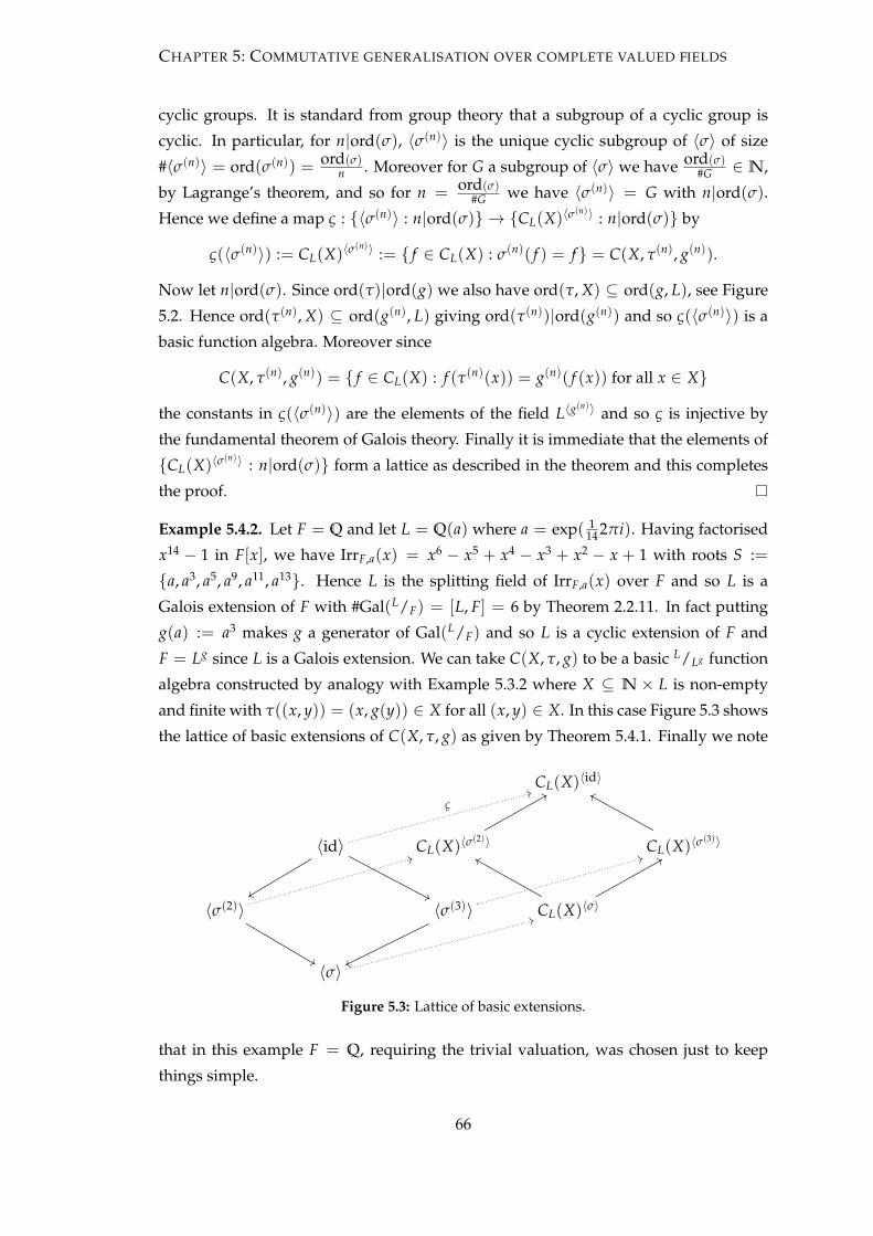
CHAPTER 5: COMMUTATIVE GENERALISATION OVER COMPLETE VALUED FIELDS
cyclic groups. It is standard from group theory that a subgroup of a cyclic group is
cyclic. In particular, for n|ord(σ), 〈σ(n)〉 is the unique cyclic subgroup of 〈σ〉 of size
#〈σ(n)〉 = ord(σ(n)) = ord(σ)n . Moreover for G a subgroup of 〈σ〉 we have ord(σ)
#G ∈ N,
by Lagrange’s theorem, and so for n = ord(σ)#G we have 〈σ(n)〉 = G with n|ord(σ).
Hence we define a map ς : {〈σ(n)〉 : n|ord(σ)} → {CL(X)〈σ(n)〉 : n|ord(σ)} by
ς(〈σ(n)〉) := CL(X)〈σ(n)〉 := { f ∈ CL(X) : σ(n)( f ) = f } = C(X, τ(n), g(n)).
Now let n|ord(σ). Since ord(τ)|ord(g) we also have ord(τ, X) ⊆ ord(g, L), see Figure
5.2. Hence ord(τ(n), X) ⊆ ord(g(n), L) giving ord(τ(n))|ord(g(n)) and so ς(〈σ(n)〉) is a
basic function algebra. Moreover since
C(X, τ(n), g(n)) = { f ∈ CL(X) : f (τ(n)(x)) = g(n)( f (x)) for all x ∈ X}
the constants in ς(〈σ(n)〉) are the elements of the field L〈g(n)〉 and so ς is injective by
the fundamental theorem of Galois theory. Finally it is immediate that the elements of
{CL(X)〈σ(n)〉 : n|ord(σ)} form a lattice as described in the theorem and this completes
the proof.
Example 5.4.2. Let F = Q and let L = Q(a) where a = exp( 114 2πi). Having factorised
x14 − 1 in F[x], we have IrrF,a(x) = x6 − x5 + x4 − x3 + x2 − x + 1 with roots S :=
{a, a3, a5, a9, a11, a13}. Hence L is the splitting field of IrrF,a(x) over F and so L is a
Galois extension of F with #Gal(L/F) = [L, F] = 6 by Theorem 2.2.11. In fact putting
g(a) := a3 makes g a generator of Gal(L/F) and so L is a cyclic extension of F and
F = Lg since L is a Galois extension. We can take C(X, τ, g) to be a basic L/Lg function
algebra constructed by analogy with Example 5.3.2 where X ⊆ N× L is non-empty
and finite with τ((x, y)) = (x, g(y)) ∈ X for all (x, y) ∈ X. In this case Figure 5.3 shows
the lattice of basic extensions of C(X, τ, g) as given by Theorem 5.4.1. Finally we note
CL(X)〈id〉
〈id〉
ς
33
yy ''
CL(X)〈σ(2)〉
88
CL(X)〈σ(3)〉
ff
〈σ(2)〉
33
&&
〈σ(3)〉
33
ww
CL(X)〈σ〉
ff 88
〈σ〉
33
Figure 5.3: Lattice of basic extensions.
that in this example F = Q, requiring the trivial valuation, was chosen just to keep
things simple.
66
CHAPTER 5: COMMUTATIVE GENERALISATION OVER COMPLETE VALUED FIELDS
5.4.2 Residue algebras
We begin with an analog of Definition 2.1.10.
Definition 5.4.3. For C(X, τ, g) a basic L/Lg function algebra in the non-Archimedean
setting, with valuation logarithm ω on L, we define:
(i) O(X, τ, g) := { f ∈ C(X, τ, g) : infx∈X ω( f (x)) ≥ 0, equivalently ‖ f ‖∞ ≤ 1};
(ii) O×(X, τ, g) := { f ∈ C(X, τ, g) : ω( f (x)) = 0, equivalently | f (x)|L = 1, ∀x ∈ X};
(iii) J (X, τ, g) := { f ∈ C(X, τ, g) : infx∈X ω( f (x)) > 0, equivalently ‖ f ‖∞ < 1};
(iv) My(X, τ, g) := { f ∈ O(X, τ, g) : ω( f (y)) > 0, equivalently | f (y)|L < 1} for
y ∈ X.
In this subsection we will mainly be interested in the following two theorems and their
proofs. The main theorem is Theorem 5.4.5 which concerns the residue algebra of par-
ticular basic function algebras. Before proving these theorems we will need to prove
several other results that are also of interest in their own right.
Theorem 5.4.4. If C(X, τ, g) is a basic L/Lg function algebra in the non-Archimedean setting
then:
(i) O(X, τ, g) is a ring;
(ii) O×(X, τ, g) is the multiplicative group of units of O(X, τ, g);
(iii) J (X, τ, g) is an ideal of O(X, τ, g);
(iv) My(X, τ, g) is a maximal ideal of O(X, τ, g) for each y ∈ X.
Theorem 5.4.5. Let F be a locally compact complete non-Archimedean field of characteristic
zero with nontrivial valuation. Let L be a finite unramified extension of F with Lg = F for some
g ∈ Gal(L/F) and let C(X, τ, g) be a basic L/F function algebra. Then there is an isometric
isomorphism
O(X, τ, g)/J (X, τ, g) ∼= C(X, τ, g)
where C(X, τ, g) is the basic L/F function algebra on (X, τ, g). Here F and L are respectively
the residue field of F and L whilst g is the residue automorphism on L induced by g. More
generally L need not be an unramified extension of F for the above to hold provided that we
impose the condition ord(τ)|ord(g) directly.
Remark 5.4.6. Concerning Theorem 5.4.5.
67

CHAPTER 5: COMMUTATIVE GENERALISATION OVER COMPLETE VALUED FIELDS
(i) The conditions in Theorem 5.4.5 imply that F contains a p-adic field, up to a posi-
tive exponent of the valuation, since by Theorem 2.1.23 the residue field F is finite
and so the valuation on F when restricted to Q can not be trivial.
(ii) Since L is finite the valuation on L is the trivial valuation. In general the quotient
norm on a residue field is the trivial valuation. In particular for a ∈ L with residue
class representative a ∈ OL we have, by Lemma 2.1.7, that
min{|a− b|L : b ∈ ML} ={
1 if a /∈ ML
0 if a ∈ ML.
(iii) To be thorough for the reader we show that g is well defined, although this is
covered in [FV02, p52]. Let a ∈ L with residue class representative a ∈ OL. For
g ∈ Gal(L/F) we obtain g ∈ Gal(L/F) by g(a) := g(a). Now let b ∈ OL with
b 6= a but b = a so that a− b ∈ ML. By Remark 2.2.6, g is an isometry on L and
so g(a)− g(b) = g(a− b) ∈ ML giving g(b) = g(b) = g(a) = g(a) and so g is
well defined.
(iv) The map g 7→ g is a homomorphism from Gal(L/F) to Gal(L/F). Indeed for a ∈ L
and g1, g2 ∈ Gal(L/F) we have
g1 ◦ g2(a) = g1 ◦ g2(a) = g1(g2(a)) = g1
(g2(a)
)= g1(g2(a)) = g1 ◦ g2(a).
Under the conditions of Theorem 5.4.5 this homomorphism becomes an isomor-
phism as per Lemma 5.4.7 below, see [FV02, p52]. In particular this ensures that
C(X, τ, g), in Theorem 5.4.5, is a basic function algebra since ord(g) = ord(g)
gives ord(τ)|ord(g).
Lemma 5.4.7. Let F be a local field, as per Remark 2.1.24, and let L be a finite unramified Galois
extension of F. Then Gal(L/F) ∼= Gal(L/F) giving ord(g) = ord(g) for all g ∈ Gal(L/F).
The following definition and lemma will be useful when proving Theorem 5.4.4. Note
that the first part of Lemma 5.4.9 makes sense even though we have yet to show that
O(X, τ, g) is a ring.
Definition 5.4.8. Let L be a complete valued field with valuation logarithm ω and let
X be a totally disconnected compact Hausdorff space.
(i) We call a map ι : X → ω(OL) a value level function.
(ii) We place a partial order on the set of all value level function by setting
ι1 ≥ ι2 if and only if for all x ∈ X we have ι1(x) ≥ ι2(x).
68

CHAPTER 5: COMMUTATIVE GENERALISATION OVER COMPLETE VALUED FIELDS
Lemma 5.4.9. Let C(X, τ, g) be a basic L/Lg function algebra in the non-Archimedean setting
with valuation logarithm ω on L and let ι : X → ω(OL) be a value level function. Then:
(i) Mι(X, τ, g) := { f ∈ C(X, τ, g) : ω( f (x)) ≥ ι(x) for all x ∈ X} is an ideal of
O(X, τ, g);
(ii) for ι′ another value level function with ι ≥ ι′ we haveMι(X, τ, g) ⊆Mι′(X, τ, g).
Proof. For (i), let f1, f2 ∈ Mι(X, τ, g) and f ∈ O(X, τ, g). Then for each x ∈ X we have
ω( f1(x) + f2(x)) ≥ min{ω( f1(x)), ω( f2(x))} ≥ ι(x) giving f1 + f2 ∈ Mι(X, τ, g) and
ω( f1(x) f (x)) = ω( f1(x)) + ω( f (x)) ≥ ω( f1(x)) ≥ ι(x) giving f1 f ∈ Mι(X, τ, g) as
required. For (ii), this is immediate.
Note, the mapping ι 7→ Mι(X, τ, g) is not assumed to be injective. We now prove
Theorem 5.4.4.
Proof of Theorem 5.4.4. For (i), note that since ω(1) = 0, ω(0) = ∞ and 1, 0 ∈ F we
have 1, 0 ∈ O(X, τ, g). Further O(X, τ, g) is closed under multiplication and addi-
tion by Lemma 5.4.9 since for the value level function that is constantly zero we have
O(X, τ, g) =M0(X, τ, g). Hence O(X, τ, g) is a ring.
For (ii), we need to show that O×(X, τ, g) = O(X, τ, g)×. Let f ∈ O(X, τ, g)×. Then
for all x ∈ X we have ω( f (x)) ≥ 0 and ω( f−1(x)) ≥ 0 since f , f−1 ∈ O(X, τ, g)×
but we also have ω( f−1(x)) = ω(( f (x))−1) = −ω( f (x)) giving ω( f (x)) = 0. Hence
O(X, τ, g)× ⊆ O×(X, τ, g). Now let f ∈ O×(X, τ, g). We have
ω( f−1(x)) = −ω( f (x)) = 0 (5.4.1)
for all x ∈ X and so it remains to show that f−1 is an element of C(X, τ, g). We have
1 = g(1) = g( f−1 f ) = g( f−1)g( f ) giving g( f−1) = (g( f ))−1 and so
f−1(τ) = ( f (τ))−1 = (g( f ))−1 = g( f−1).
For continuity let x ∈ X and (xn) be a sequence in X with limn→∞ xn = x in X. Then
by (5.4.1) we have
ω( f−1(xn)− f−1(x)) =ω( f−1(xn)− f−1(x)) + ω( f (x))
=ω(( f−1(xn)− f−1(x)) f (x))
=ω( f−1(xn) f (x)− 1)
=ω( f−1(xn)( f (x)− f (xn)))
=ω( f−1(xn)) + ω( f (x)− f (xn))
=ω( f (x)− f (xn)).
69

CHAPTER 5: COMMUTATIVE GENERALISATION OVER COMPLETE VALUED FIELDS
Therefore by the continuity of f we have limn→∞ f−1(xn) = f−1(x) from which it fol-
lows that O×(X, τ, g) ⊆ O(X, τ, g)× as required.
For (iii), taking into account that the valuation on L could be dense, J (X, τ, g) is an
ideal of O(X, τ, g) by Lemma 5.4.9 since J (X, τ, g) =⋃
n∈NM 1n(X, τ, g) noting that
1 6∈ M 1n(X, τ, g) for all n ∈N and that a union of nested ideals is an ideal.
For (iv), My(X, τ, g) is an ideal of O(X, τ, g) by Lemma 5.4.9 since My(X, τ, g) =⋃n∈NM 1
n χ{y}(X, τ, g) where χ{y} is the indicator function. Also by Lemma 5.4.9, since
1n ≥
1n χ{y} for all n ∈ N, we have J (X, τ, g) ⊆ My(X, τ, g). We now show that
My(X, τ, g) is a maximal ideal ofO(X, τ, g). Let I(X, τ, g) be a, not necessarily proper,
ideal of O(X, τ, g) with My(X, τ, g) $ I(X, τ, g). Then there is f ∈ I(X, τ, g) with
ω( f (y)) = 0. Define on X
f ′(x) :=
{0 if ω( f (x)) = 0
1 if ω( f (x)) > 0.
We show that f ′ is an element ofMy(X, τ, g) and so f ′ ∈ I(X, τ, g). For continuity let
x ∈ X and (xn) be a sequence of elements of X with limn→∞ xn = x in X. Since f is
continuous we have limn→∞ f (xn) = f (x) with respect to ω. Hence if f (x) = 0 then
there exists N ∈ N such that for all n ≥ N we have ω( f (xn)) = ω( f (xn)− f (x)) > 0.
If f (x) 6= 0 then since convergence in L is from the side, see Lemma 3.1.1, there exists
N ∈ N such that for all n ≥ N we have ω( f (xn)) = ω( f (x)). Hence in every case
there exists N ∈ N such that for all n ≥ N we have f ′(xn) = f ′(x) and so f ′ is
continuous. We need to show that f ′(τ(x)) = g( f ′(x)). Since g is an isometry on L we
have ω( f (τ(x))) = ω(g( f (x))) = ω( f (x)) giving
f ′(τ(x)) =
{0 if ω( f (τ(x))) = 0
1 if ω( f (τ(x))) > 0
= f ′(x)
=g( f ′(x))
noting that f ′ takes values only in {0, 1} ⊆ F. Now ω(1) = 0 and ω(0) = ∞ so that for
all x ∈ X we have ω( f ′(x)) ≥ 0 giving f ′ ∈ O(X, τ, g). Further since ω( f (y)) = 0 we
have ω( f ′(y)) = ω(0) = ∞ and so we have shown that f ′ ∈ My(X, τ, g) $ I(X, τ, g).
Now since I(X, τ, g) is an ideal we have f + f ′ ∈ I(X, τ, g). Moreover by the definition
of f ′, for each x ∈ X, if ω( f (x)) = 0 then ω( f ′(x)) = ω(0) = ∞ and if ω( f (x)) > 0
then ω( f ′(x)) = ω(1) = 0. Hence for all x ∈ X, ω( f (x) + f ′(x)) = 0 by Lemma 2.1.7
and so f + f ′ ∈ O×(X, τ, g) giving I(X, τ, g) = O(X, τ, g). ThereforeMy(X, τ, g) is a
maximal ideal of O(X, τ, g) and this completes the proof of Theorem 5.4.4.
The following two lemmas will be used in the proof of Theorem 5.4.5. The first of these,
Lemma 5.4.10, will be known but we provide a proof in the absence of a reference. The
70

CHAPTER 5: COMMUTATIVE GENERALISATION OVER COMPLETE VALUED FIELDS
second, Lemma 5.4.12, may be new, since I have not seen it in the literature, however it
could be known to some number theorists.
Lemma 5.4.10. Let F be a complete non-Archimedean field with a nontrivial, discrete valu-
ation and valuation logarithm ν. Let π be a prime element and R be a set of residue class
representatives for F, as shown in Theorem 2.1.13. Then, for X a compact Hausdorff space, each
f ∈ CF(X) has a unique expansion, as a series of locally constant R-valued functions, of the
form
f =∞
∑i=n
fiπi, for some n ∈ Z.
Moreover, for j ≥ n and x, y ∈ X with ν( f (x)− f (y)) > jν(π), we have fi(x) = fi(y) for
all i in the interval n ≤ i ≤ j.
Proof. Let f ∈ CF(X) and note that since X is compact, f is bounded. Hence there is
n ∈ Z such that, for all x ∈ X, ν( f (x)) ≥ nν(π). Therefore by allowing terms to be
zero where necessary and by using the unique π-power series expansion over R for
elements of F×, as shown in Theorem 2.1.13, we have for each x ∈ X
f (x) =∞
∑i=n
fi(x)πi ∈ F.
Hence for each i ≥ n we have obtained a function fi : X → R and the resulting ex-
pansion f = ∑∞i=n fiπ
i is unique. Now for j ≥ n let x, y ∈ X be such that we have
ν( f (x)− f (y)) > jν(π). If we do not have fk(x) = fk(y) for all k ≥ n then let k ≥ n
be the first integer for which fk(x) 6= fk(y). Therefore fk(x) and fk(y) are representa-
tives in OF of two different residue classes. Hence fk(x)− fk(y) 6∈ MF showing that
ν( fk(x)− fk(y)) = 0. Therefore by Lemma 2.1.7 and the definition of k we have
kν(π) =ν( fk(x)− fk(y)) + ν(πk)
=ν(( fk(x)− fk(y))πk)
=ν
(( fk(x)− fk(y))πk +
∞
∑i=k+1
fi(x)πi −∞
∑i=k+1
fi(y)πi
)
=ν
(∞
∑i=n
fi(x)πi −∞
∑i=n
fi(y)πi
)=ν( f (x)− f (y)) > jν(π).
Hence k > j giving fi(x) = fi(y) for all i in the interval n ≤ i ≤ j. Finally we show, for
all j ≥ n, that f j is a locally constant function. For x ∈ X define the following ball in F
Bjν(π)( f (x)) := {a ∈ F : ν( f (x)− a) > jν(π)}.
Then since f is continuous there exists an open subset U of X with x ∈ U such that
f (U) ⊆ Bjν(π)( f (x)). Hence for each y ∈ U we have ν( f (x)− f (y)) > jν(π) and so
71

CHAPTER 5: COMMUTATIVE GENERALISATION OVER COMPLETE VALUED FIELDS
f j(x) = f j(y). In particular f j is constant on U and this completes the proof of Lemma
5.4.10.
Lemma 5.4.10 has the following corollary which, for locally constant functions, goes
slightly further than Theorem 5.2.4 since it does not assume that X is totally discon-
nected.
Corollary 5.4.11. Let F and X be as in Lemma 5.4.10 and let LCF(X) be the set of all locally
constant F valued functions defined on X. Then LCF(X) is uniformly dense in CF(X).
Proof. For f ∈ CF(X) let f = ∑∞i=n fiπ
i be the expansion from Lemma 5.4.10. We
note that a finite sum of locally constant functions is locally constant. Hence, for each
m ≥ n, fi≤m := ∑mi=n fiπ
i is an element of LCF(X). Let ε < ∞ and m > εν(π)
. Then we
have infx∈X ν( f (x)− fi≤m(x)) = infx∈X ν(∑∞i=m+1 fi(x)πi) ≥ ν(πm+1) > mν(π) > ε as
required.
Here is the second of the two lemmas that will be used in the proof of Theorem 5.4.5.
Lemma 5.4.12. Let F and L be non-Archimedean fields with L a finite extension of F as a
valued field such that the following holds:
(i) we have Q ⊆ F and the valuation logarithm ν on F when restricted to Q is a p-adic
valuation logarithm;
(ii) the residue field F is finite and so L is also finite;
(iii) the elements of Gal(L/F) are isometric on L, noting that this is automatically satisfied if
F is complete.
Then for each g ∈ Gal(L/F) there exists a setRL,g ⊆ O×L ∪ {0} of residue class representatives
for L such that the restriction of g toRL,g is an endofunction g|RL,g : RL,g → RL,g.
Proof. Let ω be the extension of ν to L and let RL with 0 ∈ RL be an arbitrary set of
residue class representatives for L. Fix g ∈ Gal(L/F) and for a ∈ O×L denote the orbit
of a with respect to g by
〈g〉(a) := {g(n)(a) : n ∈ {1, · · · , ord(g, a)}}.
Also denote 〈g〉(a) := {g(n)(a) : n ∈ {1, · · · , ord(g, a)}} = 〈g〉(a) ⊆ L. We will show
thatRL,g ⊆ O×L ∪ {0} can be constructed fromRL. Clearly we can let 0 represent 0 and
so include 0 inRL,g. More generally we need to make sure that:
72
CHAPTER 5: COMMUTATIVE GENERALISATION OVER COMPLETE VALUED FIELDS
(1) for each a′ ∈ RL there is precisely one element a ∈ RL,g such that a = a′, that is
a = a′ + b for some b ∈ L with ω(b) > 0;
(2) for each a ∈ RL,g we have g(a) ∈ RL,g.
To this end we will show that the following useful facts hold for Lemma 5.4.12.
(a) For a1, a2 ∈ O×L either 〈g〉(a1) ∩ 〈g〉(a2) = ∅ or 〈g〉(a1) = 〈g〉(a2). Clearly, since
ord(g) is finite, if 〈g〉(a1) ∩ 〈g〉(a2) 6= ∅ then 〈g〉(a1) = 〈g〉(a2).
(b) Let a′ ∈ RL\{0}. Then there exists a ∈ O×L with a = a′ such that if a1, a2 ∈ 〈g〉(a)
with a1 6= a2 then a1 6= a2. Further since g is an isometry we have ω(a1) = 0 for
all a1 ∈ 〈g〉(a). This ensures that every residue class that has a representative in
〈g〉(a) has only one representative in 〈g〉(a).
Hence by applying (a) and (b) above we obtain RL,g as a disjoint union of the orbits of
finitely many elements form O×L ∪ {0}. Note if RF is a set of residue class represen-
tatives for F and RF ⊆ RL then with the above construction we can choose to have
RF ⊆ RL,g since g restricts to the identity map on RF. Also note that (b) is not in gen-
eral satisfied for all a ∈ O×L with a = a′. Indeed, in the case of Example 5.3.3 where
L = Q5(√
2), for a = 1 + 5√
2 we have g(a) = 1− 5√
2 6= a and yet g(a) = a = 1. We
will now prove that (a) and (b) above hold.
For (a) it is enough to confirm that 〈g〉(a) = 〈g〉(a) for all a ∈ O×L . Since g is an isom-
etry, (iii) and (iv) of Remark 5.4.6 are applicable and so we have for each n ∈ N that
g(n)(a) = g(n)(a) = g(n)(a). Hence the result follows.
For (b) we first note that, for each a′ ∈ RL\{0}, g maps residue class to residue class.
That is g restricts to a bijection g|a′ : a′ → g(a′) and g also restricts to a bijection
g|g(a′) : g(a′) → g(2)(a′) and so forth. This is because g restricts to a bijective endo-
function on ML since g has finite order and is an isometry. Now for (b) to hold we
need to check that for each a′ ∈ RL\{0} there is an a ∈ a′ such that when the forward
orbit of a, with respect to g, returns to a residue class it has visited before then it returns
to the same element of that residue class. Let a′ ∈ RL\{0} and let n be the first element
of {1, 2, · · · , ord(g, a′)} such that there exists an i ∈ {0, 1, · · · , n − 1} with g(i)(a′) in
the same residue class as g(n)(a′). Hence ω(g(i)(a′) − g(n)(a′)) > 0 and since g is an
isometry we have ω(a′ − g(n−i)(a′)) > 0 giving i = 0 by the definition of n. Therefore
g(n)(a′) = a′ + b for some b ∈ ML and g(n) restricts to g(n)|a′ : a′ → a′.
Hence for (b) to hold it is enough to show that there is a ∈ a′ which is a fixed point
with respect to g(n). To this end we more generally show that for each g ∈ Gal(L/F)
with g|a′ : a′ → a′ there is a fixed point a ∈ a′ of g. So for such a g ∈ Gal(L/F) let
m := ord(g, a′). Now recall that we have Q ⊆ F and that ν on F when restricted to Q
73
CHAPTER 5: COMMUTATIVE GENERALISATION OVER COMPLETE VALUED FIELDS
is a p-adic valuation logarithm for some prime p. Hence we have two cases, p - m and
p|m.
Suppose p - m. We have g(a′) = a′ + b for some b ∈ ML. Further then we have
g(2)(a′) =g(a′ + b) = g(a′) + g(b) = a′ + b + g(b),
g(3)(a′) =g(a′ + b + g(b)) = g(a′) + g(b) + g(2)(b) = a′ + b + g(b) + g(2)(b),...
g(m−1)(a′) =a′ + b + g(b) + g(2)(b) + · · ·+ g(m−2)(b).
Hence consider
a :=1m(a′ + g(a′) + g(2)(a′) + · · ·+ g(m−1)(a′))
=1m(ma′ + (m− 1)b + (m− 2)g(b) + · · ·+ (m− (m− 1))g(m−2)(b)).
Since Q ⊆ F we have g( 1m ) = 1
m giving g(a) = a. Moreover since p - m we have
ω(m−1) = ν(m−1) = −ν(m) = 0. Therefore
ω(a− a′) =ω
(1m((m− 1)b + (m− 2)g(b) + (m− 3)g(2)(b) + · · ·+ g(m−2)(b))
)=0 + ω((m− 1)b + (m− 2)g(b) + (m− 3)g(2)(b) + · · ·+ g(m−2)(b))
≥min{ω((m− 1)b), ω((m− 2)g(b)), ω((m− 3)g(2)(b)), · · · , ω(g(m−2)(b))}
=ω(g(m−2)(b)) = ω(b) > 0.
Hence a is an element of a′ with g(a) = a as required.
Suppose p|m. Then there is n, m′ ∈ N such that m = pnm′ with p - m′. Hence
ord(g(pn−1m′), a′) = p. Now suppose that the following holds.
(b2) Let a0 ∈ O×L . Then for each g′ ∈ Gal(L/F) with g′|a0 : a0 → a0 and ord(g′, a0) = p
there is a fixed point a1 ∈ a0 of g′.
Then by applying (b2) there is a1 ∈ a′ which is a fixed point of g(pn−1m′) and so we have
ord(g, a1)|pn−1m′. By repeated application of (b2) we can obtain an element an ∈ a′
such that ord(g, an)|m′. Now, since the set RL was an arbitrary set of residue class
representatives for L and an represents a′, we can apply the case p - m for an to obtain
a ∈ an = a′ with g(a) = a as required.
It remains to show that (b2) holds. So let a0 ∈ O×L and g′ ∈ Gal(L/F) satisfy the
conditions of (b2). Hence for some b ∈ ML we have
g′(a0) =a0 + b,
g′(2)(a0) =a0 + b + g′(b),...
g′(p−1)(a0) =a0 + b + g′(b) + · · ·+ g′(p−2)(b).
74
CHAPTER 5: COMMUTATIVE GENERALISATION OVER COMPLETE VALUED FIELDS
Define b1 := b, b2 := b + g′(b), · · · , bp−1 := b + g′(b) + · · ·+ g′(p−2)(b) and note that
for all i ∈ {1, · · · , p− 1} we have
ω(bi) ≥ min{ω(b), ω(g′(b)), · · · , ω(g′(p−2)(b))} = ω(b) > 0. (5.4.2)
Now since ω|Q is the p-adic valuation logarithm νp we have Fp ⊆ L. Therefore since L
is a finite field we have #L = pk for some k ∈N. Hence we consider
a1 :=(a0g′(a0)g′(2)(a0) · · · g′(p−1)(a0))pk−1
=(a0(a0 + b1)(a0 + b2) · · · (a0 + bp−1))pk−1
=(ap0 + a0b1(a0 + b2) · · · (a0 + bp−1) + a2
0b2(a0 + b3) · · · (a0 + bp−1) + · · ·
· · ·+ ap−10 bp−1)
pk−1.
Now, by Lemma 2.1.7 and (5.4.2), we have
ω(a0b1(a0 + b2) · · · (a0 + bp−1)) =ω(a0) + ω(b1) + ω(a0 + b2) + · · ·
· · ·+ ω(a0 + bp−1)
=0 + ω(b1) + 0 + · · ·+ 0
≥ω(b) > 0.
The same inequality holds for later terms in the above expansion on a1, hence for
c := a0b1(a0 + b2) · · · (a0 + bp−1) + a20b2(a0 + b3) · · · (a0 + bp−1) + · · ·+ ap−1
0 bp−1
we have ω(c) > 0. This gives
a1 = (ap0 + c)pk−1
= apk
0 +pk−1
∑i=1
(pk−1
i
)ap(pk−1−i)
0 ci
such that for each i ∈ {1, · · · , pk−1} we have
ω
((pk−1
i
)ap(pk−1−i)
0 ci)=ω
((pk−1
i
))+ p(pk−1 − i)ω(a0) + iω(c)
=ω
((pk−1
i
))+ 0 + iω(c) > 0
noting that ω((pk−1
i ))≥ 0 since ω|Q is the p-adic valuation logarithm νp. Hence for
c′ := ∑pk−1
i=1 (pk−1
i )ap(pk−1−i)0 ci we have ω(c′) > 0. Further since #L× = pk − 1 we have
a0pk−1 = 1 by Lagrange’s theorem. In particular a1 = apk
0 + c′ = a0pk+ 0 = a0 giving
a1 ∈ a0 and since a1 = (a0g′(a0)g′(2)(a0) · · · g′(p−1)(a0))pk−1with ord(g′, a0) = p we
have g′(a1) = a1 as required. This completes the proof of Lemma 5.4.12.
We will now prove Theorem 5.4.5.
75
CHAPTER 5: COMMUTATIVE GENERALISATION OVER COMPLETE VALUED FIELDS
Proof of Theorem 5.4.5. For f ∈ O(X, τ, g) let f := f + J (X, τ, g) denote the quotient
class to which f belongs and let π be a prime element of L. Note,O(X, τ, g)/J (X, τ, g)
is endowed with the usual quotient operations and the quotient norm which in this case
gives the trivial valuation. We begin by establishing a set R(X, τ, g) ⊆ O(X, τ, g) of
quotient class representatives for O(X, τ, g)/J (X, τ, g). By Lemma 5.4.12 there is a set
RL,g of residue class representatives for L such that g|RL,g : RL,g → RL,g. Furthermore
by Lemma 5.4.10 every f ∈ CL(X) has a unique expansion of the form
f =∞
∑i=n
fiπi, for some n ∈ Z, (5.4.3)
where, for each i ≥ n, fi : X → RL,g is a locally constant function. Hence, using
expansion (5.4.3), for f ∈ O(X, τ, g) we have
f0 ◦ τ + h ◦ τ = f ◦ τ = g ◦ f = g ◦ f0 + g ◦ h
where h := ∑∞i=1 fiπ
i with ω(h(x)) > 0 for all x ∈ X. Now note that τ : X → X and
g|RL,g : RL,g → RL,g give f0 ◦ τ : X → RL,g and g ◦ f0 : X → RL,g. Further since g is
an isometry on L we have ω(h ◦ τ(x)) > 0 and ω(g ◦ h(x)) > 0 for all x ∈ X. Hence
since the expansion of f ◦ τ in the for of (5.4.3) is unique we have f0 ◦ τ = g ◦ f0 and
h ◦ τ = g ◦ h. Moreover f0 is continuous since locally constant and, for x ∈ X,
ω( f0(x)) =
{∞ if f0(x) = 0
0 if f0(x) 6= 0.
In particular we have f0 ∈ O(X, τ, g). Hence we also have h = f − f0 ∈ O(X, τ, g) since
O(X, τ, g) is a ring. But since ω(h(x)) > 0 for all x ∈ X we in fact have h ∈ J (X, τ, g)
giving
f = f0.
Now by the uniqueness of expansions in the form of (5.4.3) and since J (X, τ, g) is an
ideal we have for any other element f ′ = f ′0 + h′ ∈ O(X, τ, g) that f ′ = f if and only if
f ′0 = f0. Hence using expansion (5.4.3) we define
R(X, τ, g) :=
{f0 : f =
∞
∑i=0
fiπi ∈ O(X, τ, g)
}
noting that 0 ∈ R(X, τ, g) since 0 ∈ RL,g and 0 ∈ O(X, τ, g). We now define a map
φ : O(X, τ, g)/J (X, τ, g)→ C(X, τ, g) by
φ( f ) = φ( f0) = φ( f0 + J (X, τ, g)) := f0
where for x ∈ X we define f0(x) := f0(x) = f0(x) +ML. We show that φ is a ring
isomorphism by checking that:
76

CHAPTER 5: COMMUTATIVE GENERALISATION OVER COMPLETE VALUED FIELDS
(i) for all f ∈ O(X, τ, g)/J (X, τ, g) we have f0 ∈ C(X, τ, g);
(ii) φ is multiplicative, linear and φ(1) = 1;
(iii) ker(φ) = {0} ensuring that φ is injective;
(iv) φ is surjective.
For (i), since f0 is a locally constant function on X we have f0 ∈ CL(X). Furthermore
we have already shown above that f0 ◦ τ = g ◦ f0. Hence for each x ∈ X we have
f0(τ(x)) = f0(τ(x)) = g( f0(x)) = g(
f0(x))= g
(f0(x)
)and so f0 ∈ C(X, τ, g).
For (ii), let f , f ′ ∈ O(X, τ, g)/J (X, τ, g). We show that φ is multiplicative. Set h := f0 f ′0giving f0 f ′0 = h0 + h′ with h′ ∈ J (X, τ, g) and f0, f ′0, h0 ∈ R(X, τ, g). Hence for each
x ∈ X we have h′(x) ∈ ML. Therefore for each x ∈ X we have
φ( f f ′)(x) = φ( f0 f ′0)(x) =φ( f0 f ′0)(x)
=φ(h0)(x)
=h0(x)
=h0(x)
=h0(x) + h′(x)
= f0(x) f ′0(x)
= f0(x) f ′0(x)
=(φ( f0)φ( f ′0))(x) = (φ( f )φ( f ′))(x).
Linearity, φ( f + f ′) = φ( f ) + φ( f ′), is shown in much the same way. Showing that
φ(1) = 1 is almost immediate. Let 10 be the representative in RL,g of 1. Then we have
10 ∈ R(X, τ, g) giving φ(1) = φ(10) = 10 = 1 as required. In fact we can always choose
RL,g such that 10 = 1.
For (iii), let f ∈ O(X, τ, g). If for all x ∈ X we have φ( f0)(x) = f0(x) = 0 then
ω( f0(x)) > 0 for all x ∈ X giving f0 ∈ J (X, τ, g). Hence f0 = 0 and so ker(φ) = {0}.In fact since f0 is an element ofR(X, τ, g) we have f0 = 0 in this case.
For (iv), given f ∈ C(X, τ, g) and x ∈ X we have f (x) = a0(x) +ML for some element
a0(x) ofRL,g sinceRL,g is a set of residue class representatives for L. Since the valuation
on L is the trivial valuation, f is a locally constant function and hence, when viewed as
a function on X, so is a0. Therefore a0 is a continuous OL valued function noting that
RL,g ⊆ OL. Further since f ∈ C(X, τ, g) we have for each x ∈ X that
a0(τ(x)) = f (τ(x)) = g( f (x)) = g(
a0(x))= g(a0(x)).
Now because g|RL,g : RL,g → RL,g we have g(a0(x)) ∈ RL,g giving a0(τ(x)) = g(a0(x))
for all x ∈ X. Hence, as a function on X, a0 ∈ O(X, τ, g) and so a0 ∈ R(X, τ, g) with
77
CHAPTER 5: COMMUTATIVE GENERALISATION OVER COMPLETE VALUED FIELDS
φ(a0) = a0 = f as required. Finally, since the valuation on L is the trivial valuation,
the sup norm on C(X, τ, g) is the trivial norm. Therefore it is immediate that φ is an
isometry and this completes the proof of Theorem 5.4.5.
The last result of this section follows easily from the preceding results.
Corollary 5.4.13. Let F, L and g ∈ Gal(L/F) conform to Lemma 5.4.12 with F and L having
complete nontrivial discrete valuations and let C(X, τ, g) be a basic L/Lg function algebra.
Further letR(X, τ, g) ⊆ O(X, τ, g) be the subset of all locally constantRL,g valued functions.
If there is a prime element π of L such that g(π) = π then each f ∈ C(X, τ, g)\{0} has a
unique series expansion of the form
f =∞
∑i=n
fiπi, for some n ∈ Z,
where for each i ≥ n we have fi ∈ R(X, τ, g). In particular the subset of all locally constant
functions, LC(X, τ, g) ⊆ C(X, τ, g), is uniformly dense in C(X, τ, g).
Remark 5.4.14. For L an unramified extension of F, every prime element π ∈ F is a
prime element of L with g(π) = π. In particular Corollary 5.4.13 holds when L is a
finite unramified extension of Qp as is the case for examples 5.3.3 and 5.3.4.
Proof of Corollary 5.4.13. Let f be an element of C(X, τ, g)\{0} and let π be a prime
element of L with g(π) = π. By Lemma 5.4.10 f has a unique series expansion of the
form
f =∞
∑i=n
fiπi, for some n ∈ Z,
with fn 6= 0 and fi : X → RL,g a locally constant function for all i ≥ n. Hence
∞
∑i=n
fi ◦ τπi = f ◦ τ = g ◦ f =∞
∑i=n
(g ◦ fi)(g(π))i =∞
∑i=n
g ◦ fiπi.
Therefore since g restricts to an endofunction on RL,g and by the uniqueness of the
expansion we have fi ◦ τ = g ◦ fi for all i ≥ n. Hence fi is an element ofR(X, τ, g) for all
i ≥ n and for each m ∈ N we have ∑n+m−1i=n fiπ
i ∈ C(X, τ, g). Finally(
∑n+m−1i=n fiπ
i)
mis a sequence of locally constant functions which converges uniformly to f as required.
This brings us to the end of Chapter 5. In the next chapter we will see that L/Lg function
algebras have a part to play in representation theory.
78

CHAPTER 6
Representation theory
The first section of this chapter introduces several results from the theory of Banach
rings and Banach F-algebras that we will use later in the chapter. These results have
been taken from [Ber90, Ch1]. However I have provided a thorough proof of each result
in order to give significantly more detail than [Ber90] since some of them may not be
widely known. The second section begins by recalling which Banach F-algebras can be
represented by complex uniform algebras or real function algebras in the Archimedean
setting and one such result in the non-Archimedean setting provided by [Ber90] is also
noted. We then develop this theory further by identifying a large class of Banach F-
algebras that can be represented by L/Lg function algebras. The resulting representa-
tion theorem is the main result of interest in this chapter and the rest of the chapter is
given over to the proof of the theorem.
6.1 Further Banach rings and Banach F-algebras
Since the definition of a Banach ring was given in Definition 3.2.1 we begin with the
first lemma.
Lemma 6.1.1. Let R be a Banach ring and let r ∈ R be positive. Define
R〈r−1T〉 := { f =∞
∑i=0
aiTi : ai ∈ R and∞
∑i=0‖ai‖Rri < ∞}.
Then with the Cauchy product and usual addition:
(i) we have that R〈r−1T〉 is a Banach ring with respect to the norm
‖ f ‖R,r :=∞
∑i=0‖ai‖Rri;
(ii) for a ∈ R we have 1− aT invertible in R〈r−1T〉 if and only if ∑∞i=0 ‖ai‖Rri < ∞.
79
CHAPTER 6: REPRESENTATION THEORY
Proof. For (i), let f1 = ∑∞i=0 aiTi and f2 = ∑∞
i=0 biTi be elements of R〈r−1T〉. Then
‖ f1 + f2‖R,r =
∥∥∥∥∥ ∞
∑i=0
(ai + bi)Ti
∥∥∥∥∥R,r
=∞
∑i=0‖ai + bi‖Rri
≤∞
∑i=0
(‖ai‖R + ‖bi‖R) ri
=∞
∑i=0‖ai‖Rri +
∞
∑i=0‖bi‖Rri
=‖ f1‖R,r + ‖ f2‖R,r < ∞
showing that R〈r−1T〉 is closed under addition and that the triangle inequality holds
for ‖ · ‖R,r. Clearly ‖ f ‖R,r = 0 if and only if f = 0. Further
‖ f1 f2‖R,r =
∥∥∥∥∥ ∞
∑i=0
(i
∑k=0
akbi−k
)Ti
∥∥∥∥∥R,r
=∞
∑i=0
∥∥∥∥∥ i
∑k=0
akbi−k
∥∥∥∥∥R
ri
≤∞
∑i=0
(i
∑k=0‖ak‖R‖bi−k‖R
)ri
=
(∞
∑i=0‖ai‖Rri
)(∞
∑i=0‖bi‖Rri
), by Mertens’ Theorem, see [Apo74, p204]
=‖ f1‖R,r‖ f2‖R,r < ∞
showing that R〈r−1T〉 is closed under multiplication and ‖ · ‖R,r is sub-multiplicative.
Furthermore we have 1R,r = 1RT0 which gives ‖1R,r‖R,r = ‖1R‖Rr0 = 1 and similarly
‖ − 1R,r‖R,r = ‖ − 1R‖Rr0 = 1.
We now show that R〈r−1T〉 is complete. Let(∑∞
i=0 ai,nTi)n be a Cauchy sequence in
R〈r−1T〉. Then for k ∈ N0 and ε > 0 there exists M ∈ N such that for all m, m′ ≥ M
we have ‖∑∞i=0 ai,mTi − ∑∞
i=0 ai,m′Ti‖R,r = ∑∞i=0 ‖ai,m − ai,m′‖Rri < εrk. Hence for all
m, m′ ≥ M we have ‖ak,m − ak,m′‖R < ε and so for all k ∈ N0, (ak,n)n is a Cauchy
sequence in R. Since R is a Banach ring (ak,n)n converges to some bk ∈ R.
We show that ∑∞i=0 biTi is an element of R〈r−1T〉. Let ε0 > 0. Then there exists M ∈ N
such that for all m ≥ M we have∥∥∥∥∥ ∞
∑i=0
ai,mTi
∥∥∥∥∥R,r
≤∥∥∥∥∥ ∞
∑i=0
ai,mTi −∞
∑i=0
ai,MTi
∥∥∥∥∥R,r
+
∥∥∥∥∥ ∞
∑i=0
ai,MTi
∥∥∥∥∥R,r
<ε0 +
∥∥∥∥∥ ∞
∑i=0
ai,MTi
∥∥∥∥∥R,r
< ∞.
80
CHAPTER 6: REPRESENTATION THEORY
Now let N ∈ N0 and ε > 0. Since for each k ∈ N0, (ak,n)n is a Cauchy sequence in R
with limit bk, there is M′ ∈N such that for all m′ ≥ M′ we have ∑Ni=0 ‖bi− ai,m′‖Rri < ε.
Hence letting m0 ≥ max{M, M′} gives∥∥∥∥∥ N
∑i=0
biTi
∥∥∥∥∥R,r
=
∥∥∥∥∥ N
∑i=0
biTi −N
∑i=0
ai,m0 Ti +N
∑i=0
ai,m0 Ti
∥∥∥∥∥R,r
≤∥∥∥∥∥ N
∑i=0
(bi − ai,m0)Ti
∥∥∥∥∥R,r
+
∥∥∥∥∥ ∞
∑i=0
ai,m0 Ti
∥∥∥∥∥R,r
<ε + ε0 +
∥∥∥∥∥ ∞
∑i=0
ai,MTi
∥∥∥∥∥R,r
.
Since ε > 0 was arbitrary we have ‖∑Ni=0 biTi‖R,r ≤ ε0 + ‖∑∞
i=0 ai,MTi‖R,r. Since
this holds for each N ∈ N0 we have ‖∑∞i=0 biTi‖R,r ≤ ε0 + ‖∑∞
i=0 ai,MTi‖R,r giving
∑∞i=0 biTi ∈ R〈r−1T〉 as required.
Let ε > 0. We will show, for large enough n ∈ N, that ‖∑∞i=0 ai,nTi −∑∞
i=0 biTi‖R,r < ε
and so R〈r−1T〉 is complete. Since(∑∞
i=0 ai,nTi)n is a Cauchy sequence there exists
M1 ∈N such that for all m, n ≥ M1 we have ‖∑∞i=0(ai,n − ai,m)Ti‖R,r < ε/4.
Let n ≥ M1. Since ∑∞i=0 ai,nTi and ∑∞
i=0 biTi are elements of R〈r−1T〉 there exists N ∈N
such that ‖∑∞i=N+1 ai,nTi‖R,r < ε/4 and ‖∑∞
i=N+1 biTi‖R,r < ε/4.
Since for each i ∈ N0, (ai,m)m is a Cauchy sequence in R with limit bi, there is M2 ∈ N
such that for all m ≥ M2 we have ‖∑Ni=0(ai,m − bi)Ti‖R,r = ∑N
i=0 ‖ai,m − bi‖Rri < ε/4.
Let m = max{M1, M2} and define cn := ‖∑∞i=0 ai,nTi −∑∞
i=0 biTi‖R,r, then
cn =
∥∥∥∥∥ ∞
∑i=N+1
ai,nTi +N
∑i=0
(ai,n − ai,m)Ti +N
∑i=0
(ai,m − bi)Ti −∞
∑i=N+1
biTi
∥∥∥∥∥R,r
<ε/4 + ε/4 + ε/4 + ε/4 = ε as required.
For (ii), the result is obvious for a = 0 and so suppose a 6= 0. If ∑∞i=0 ‖ai‖Rri < ∞ then
∑∞i=0 aiTi is an element of R〈r−1T〉 and by the definition of the Cauchy product we have(
∞
∑i=0
aiTi
)(1− aT) =(a01R)T0 +
∞
∑i=1
(ai1R + ai−1(−a))Ti
=1RT0 +∞
∑i=1
ai−1(a + (−a))Ti
=1RT0 = 1R,r = 1.
Similarly this holds for (1− aT)(∑∞i=0 aiTi) and so 1− aT is invertible.
Now conversely if 1− aT is invertible in R〈r−1T〉 then for ∑∞i=0 biTi the inverse of 1− aT
in R〈r−1T〉 we have by the definition of the Cauchy product
1R,r =
(∞
∑i=0
biTi
)(1− aT) = (b01R)T0 +
∞
∑i=1
(bi1R + bi−1(−a))Ti.
81

CHAPTER 6: REPRESENTATION THEORY
Hence b0 = 1R = a0 and, for each i ∈N, 0 = bi + bi−1(−a) giving
bi−1a = bi + bi−1a + bi−1(−a) = bi + bi−1(a + (−a)) = bi.
Therefore for each i ∈ N, bi = bi−1a with b0 = 1R giving bi = ai by induction. Hence
∑∞i=0 aiTi = ∑∞
i=0 biTi is an element of R〈r−1T〉 and so ∑∞i=0 ‖ai‖Rri < ∞ as required.
Remark 6.1.2. Since R〈r−1T〉 extends R as a ring and by the definition of the Cauchy
product it is immediate that R〈r−1T〉 is commutative if and only if R is commutative.
Similarly by the definition of the norm ‖ · ‖A,r and the Cauchy product, if A is a unital
Banach F-algebra then A〈r−1T〉 is also a unital Banach F-algebra. These details are
easily checked.
The following definitions will be used many times in this chapter.
Definition 6.1.3. Let R be a Banach ring. A bounded multiplicative seminorm on R is a
map | · | : R→ R taking non-negative values that is:
(1) bounded, |a| ≤ ‖a‖R for all a ∈ R, but not constantly zero on R;
(2) multiplicative, |ab| = |a||b| for all a, b ∈ R and hence |1R| = 1 by setting a = 1R
and b 6∈ ker(| · |);
(3) a seminorm and so | · | also satisfies the triangle inequality and 0 ∈ ker(| · |) but
the kernel is not assumed to be a singleton.
Definition 6.1.4. Let F be a complete non-Archimedean field and let A be a commuta-
tive unital Banach F-algebra. In this chapter M0(A) will denote the set of all proper
closed prime ideals of A that are the kernels of bounded multiplicative seminorms on
A. For x0 ∈ M0(A), or any proper closed ideal of A, we will denote the quotient norm
on A/x0 by | · |x0 that is |a + x0|x0 := inf{‖a + b‖A : b ∈ x0} for a ∈ A.
We now proceed with a number of Lemmas. In particular towards the end of Section
6.1 it will be show thatM0(A) is always nonempty.
Lemma 6.1.5. Let A be a unital Banach F-algebra. If | · | is a bounded multiplicative seminorm
on A as a Banach ring then we have |α| = |α|F for all α ∈ F. Hence since | · | is multiplicative
it is also a vector space seminorm, that is |αa| = |α|F|a| for all a ∈ A and α ∈ F.
Proof. For α ∈ F× we first note that 1 = |1A| = |αα−1| = |α||α−1| and so |α| 6= 0 and
|α−1| = |α|−1. Similarly |α−1|F = |α|−1F since | · |F is a valuation. Moreover since | · | is
bounded we have |α| ≤ ‖α1A‖A = |α|F‖1A‖A = |α|F. Since this holds for all α ∈ F×
we also have |α−1| ≤ |α−1|F giving |α|F ≤ |α| and so |α| = |α|F for all α ∈ F.
82
CHAPTER 6: REPRESENTATION THEORY
Lemma 6.1.6. Let F and A be as in Definition 6.1.4. For x0 ∈ M0(A), or any proper closed
ideal of A, the following holds:
(i) the quotient ring A/x0 has F ⊆ A/x0 and is an integral domain if x0 is prime;
(ii) the quotient norm is such that |α + x0|x0 = |α|F for all α ∈ F;
(iii) the quotient norm | · |x0 is an F-vector space norm on A/x0, opposed to being merely a
seminorm, and it is sub-multiplicative;
(iv) if ‖ · ‖A is square preserving, that is ‖a2‖A = ‖a‖2A for all a ∈ A, then both ‖ · ‖A and
| · |x0 observe the strong triangle inequality noting that F is non-Archimedean;
(v) by way of the map a 7→ |a + x0|x0 , as a seminorm on A, | · |x0 is bounded.
Proof. For (i), if a1 + x0, a2 + x0 ∈ A/x0 with (a1 + x0)(a2 + x0) = a1a2 + x0 = 0 + x0
then we have a1a2 ∈ x0. Hence if x0 is a prime ideal of A then at least one of a1 + x0
and a2 + x0 is equal to 0 + x0 and so A/x0 is an integral domain. It is immediate that
A/x0 has a subset that is an isomorphic copy of F since x0 is a proper ideal of A.
For (ii), we first show that |1 + x0|x0 = 1. Note that |1 + x0|x0 ≤ ‖1‖A = 1 since 0 ∈ x0.
So now suppose toward a contradiction that there is b ∈ x0 such that ‖1 + b‖A < 1.
We have for all n ∈ N that bn := −((1 + b)n − 1) is an element of x0 since x0 is an
ideal of A. But ‖1− bn‖A = ‖(1 + b)n‖A ≤ ‖1 + b‖nA with limn→∞ ‖1 + b‖n
A = 0 and
so 1 is an element of x0 since x0 is closed which contradicts x0 being a proper ideal
of A. We conclude that ‖1 + b‖A ≥ 1 for all b ∈ x0 and so |1 + x0|x0 ≥ 1. Hence
|1 + x0|x0 = 1 by the above. Now for α ∈ F× we have x0 = αx0 since α is invertible
where αx0 := {αb : b ∈ x0}. Hence
|α + x0|x0 = inf{‖α + b‖A : b ∈ x0}
= inf{‖α + αb‖A : b ∈ x0}
= inf{|α|F‖1 + b‖A : b ∈ x0}
=|α|F|1 + x0|x0 = |α|F
as required. In a similar way for a ∈ A one shows that |αa + x0|x0 = |α|F|a + x0|x0 .
For (iii), we note that | · |x0 is a norm on A/x0 because x0 is closed as a subset of A so
that for a ∈ A\x0 there is ε > 0 with ‖a + b‖A ≥ ε for all b ∈ x0 giving |a + x0|x0 ≥ ε.
We now show that | · |x0 is sub-multiplicative. For a1, a2 ∈ A we have
|a1a2 + x0|x0 = inf{‖a1a2 + b‖A : b ∈ x0}
≤ inf{‖a1a2 + a1b2 + a2b1 + b1b2‖A : b1, b2 ∈ x0}
≤ inf{‖a1 + b1‖A‖a2 + b2‖A : b1, b2 ∈ x0}
=|a1 + x0|x0 |a2 + x0|x0 .
83
CHAPTER 6: REPRESENTATION THEORY
For (iv), suppose ‖ · ‖A is square preserving. In this case the proof of Theorem 2.1.2
also works for A and so ‖ · ‖A observes the strong triangle inequality, see [Sch06, p18]
for details. Hence for a1, a2 ∈ A we also have
|a1 + a2 + x0|x0 = inf{‖a1 + a2 + b‖A : b ∈ x0}
= inf{‖a1 + b1 + a2 + b2‖A : b1, b2 ∈ x0}
≤ inf{max{‖a1 + b1‖A, ‖a2 + b2‖A} : b1, b2 ∈ x0}
=max{inf{‖a1 + b1‖A : b1 ∈ x0}, inf{‖a2 + b2‖A : b2 ∈ x0}}
=max{|a1 + x0|x0 , |a2 + x0|x0}.
For (v), since we have 0 ∈ x0 it is immediate that |a + x0|x0 ≤ ‖a‖A for all a ∈ A.
Lemma 6.1.7. Let R be a commutative Banach ring. Then:
(i) if a ∈ R has ‖1− a‖R < 1 then a is invertible in R;
(ii) for I a proper ideal of R the closure J of I, as a subset of R, is a proper ideal of R;
(iii) each non-invertible element of R is an element of some maximal ideal of R. The maximal
ideals of R are proper, closed and prime.
Proof. For (i), for a ∈ R with ‖1− a‖R < 1 let δ > 0 be such that ‖1− a‖R < δ < 1.
Then setting b := 1− a gives ‖bn‖R ≤ ‖b‖nR < δn < 1 for all n ∈ N. Therefore we have
∑mn=0 ‖bn‖R < ∑∞
n=0 δn = 11−δ for each m ∈ N and so ∑∞
n=0 bn ∈ R since R is complete.
Moreover∥∥∥∥∥(1− b)∞
∑n=0
bn − 1
∥∥∥∥∥R
=
∥∥∥∥∥(1− b)∞
∑n=0
bn − (1− b)m
∑n=0
bn + (1− b)m
∑n=0
bn − 1
∥∥∥∥∥R
≤(
∞
∑n=m+1
‖bn‖R
)‖1− b‖R + ‖bm+1‖R.
Hence a is invertible in R since 1− b = 1− (1− a) = a and
limm→∞
((∞
∑n=m+1
‖bn‖R
)‖1− b‖R + ‖bm+1‖R
)= 0.
For (ii), let I be a proper ideal of R and J its closure as a subset. For a, b ∈ J there are
sequences (an), (bn) of elements of I converging to a and b respectively with respect to
‖ · ‖R. Hence for a′ ∈ R, (a′an) is a sequence in I with ‖a′a− a′an‖R ≤ ‖a′‖R‖a− an‖R
for each n ∈ N and so a′a ∈ J since limn→∞ ‖a − an‖R = 0. Similarly (an + bn) is a
sequence in I with ‖(a + b)− (an + bn)‖R ≤ ‖a− an‖R + ‖b− bn‖R for each n ∈N and
so a+ b ∈ J. Hence J is an ideal of R. Now since I is a proper ideal of R each element an
of the sequence (an) is not invertible and so ‖1− an‖R ≥ 1 for all n ∈ N by (i). Hence
84
CHAPTER 6: REPRESENTATION THEORY
1 ≤ ‖1− a + a− an‖R ≤ ‖1− a‖R + ‖a− an‖R for all n ∈ N and so ‖1− a‖R ≥ 1 for
all a ∈ J giving 1 6∈ J. Hence J is proper.
For (iii), let a be a non-invertible element of R noting that we can always take a = 0.
The principal ideal Ia := aR is proper since for all b ∈ R, ab 6= 1. By Zorn’s lemma Ia is
a subset of some maximal ideal Ja of R. Every maximal ideal J of R is proper and prime,
noting that R/J is a field or by other means, and closed as a subset of R by (ii).
Remark 6.1.8. We note that if A is a commutative unital Banach F-algebra then Lemma
6.1.7 applies to A and A〈r−1T〉 for each r > 0.
Lemma 6.1.9. Let F be a complete non-Archimedean field and let A be a commutative unital
Banach F-algebra with maximal ideal m0. Let S(A) denote the set of all norms on the field
A/m0 that are also unital bounded seminorms on A as a Banach ring. That is if | · | is an
element of S(A) then |1| = 1 and | · | conforms to Definition 6.1.3 except it need not be
multiplicative merely sub-multiplicative. It follows that:
(i) the set S(A) is non-empty;
(ii) for | · | ∈ S(A), A/m0 the completion of A/m0 with respect to | · |, r > 0 and a ∈ A/m0,
if a− T is non-invertible in A/m0〈r−1T〉 then there is | · |′ ∈ S(A) with |a|′ ≤ r and
|b|′ ≤ |b| for all b ∈ A/m0.
Proof. For (i), we note that the quotient norm | · |m0 is an element of S(A) since (iii) of
Lemma 6.1.7 shows that (ii), (iii) and (v) of Lemma 6.1.6 apply to | · |m0 .
For (ii), suppose that a− T is non-invertible in A/m0〈r−1T〉. Then a− T is an element
of some maximal ideal J of A/m0〈r−1T〉 by Lemma 6.1.7. Hence the quotient norm | · |Jon A/m0〈r−1T〉/J is an element of S(A/m0〈r−1T〉) by Lemma 6.1.6. Therefore since J
is closed and A/m0 is a field, |a′|′ := |a′ + J|J , for a′ ∈ A/m0, defines a norm on A/m0.
Since | · |J is an element of S(A/m0〈r−1T〉) we have that | · |′ is unital as a seminorm
on A. Similarly since | · |J is bounded as a seminorm on A/m0〈r−1T〉 we have for all
a′ ∈ A that
|a′ + m0|′ = |(a′ + m0) + J|J ≤ ‖a′ + m0‖A/m0,r = |a′ + m0| ≤ ‖a′‖A (6.1.1)
noting that | · | is an element of S(A). Hence | · |′ is bounded as a seminorm on A and
so | · |′ is an element of S(A). Further since a− T is an element of J we have
|a|′ = |a + J|J = |T + J|J ≤ ‖T‖A/m0,r = r.
Finally we have |b|′ ≤ |b| for all b ∈ A/m0 by (6.1.1).
The following Lemma will be particularly useful in Section 6.2.
85
CHAPTER 6: REPRESENTATION THEORY
Lemma 6.1.10. Let F be a complete non-Archimedean field and let A be a commutative unital
Banach F-algebra. With reference to Definition 6.1.4 the following holds:
(i) the setM0(A) is non-empty since every maximal ideal of A is an element ofM0(A);
(ii) an element a ∈ A is invertible if and only if a + x0 6= 0 + x0 for all x0 ∈ M0(A).
Proof. Whilst this proof provides more detail, much of the following has been taken
from [Ber90, Ch1]. For (i), let m0 be a maximal ideal of A. Hence the quotient ring
A/m0 is a field. Let S(A) be as in Lemma 6.1.9 and note therefore that S(A) is non-
empty. We put a partial order on S(A) by | · | . | · |′ if and only if |a + m0| ≤ |a + m0|′
for all a + m0 ∈ A/m0. Now let E be a chain in S(A), that is E is a subset of S(A) such
that . restricts to a total order on E. Define a map | · |E : A/m0 → R by
|a + m0|E := inf{|a + m0| : | · | ∈ E}.
We will show that | · |E is a lower bound for E in S(A). It is immediate from the defini-
tion of | · |E that it is unital and bounded since all of the elements of E are. Hence it suf-
fices to show that | · |E is a sub-multiplicative norm on A/m0. Clearly |0 + m0|E = 0 so,
simplifying our notation slightly, let a be an element of A/m×0 . We show that |a|E 6= 0.
Let | · | be an element of E and suppose towards a contradiction that there is | · |′ ∈ E
such that |a|′ < min{|a|, |a−1|−1}. Then
1 = |1|′ = |aa−1|′ ≤ |a|′|a−1|′ < |a−1|−1|a−1|′.
Hence by the above we have |a−1| < |a−1|′ and |a|′ < |a| giving | · |′ 6. | · | and | · | 6. | · |′
which contradicts both | · | and | · |′ being elements of E. Therefore for all | · |′ ∈ E we
have |a|′ ≥ min{|a|, |a−1|−1}. In particular |a|E 6= 0. Now for a, b ∈ A/m0 we have
|a + b|E = inf{|a + b| : | · | ∈ E}
≤ inf{|a|+ |b| : | · | ∈ E}
= inf{|a|+ |b|′ : | · |, | · |′ ∈ E}, †
=|a|E + |b|E,
where line † follows from the line above it because if | · | . | · |′ then |a|+ |b| ≤ |a|+ |b|′.Hence the triangle inequality holds for | · |E. Similarly we have |ab|E ≤ |a|E|b|E and so
| · |E is sub-multiplicative as required. Hence | · |E is a lower bound for E in S(A).
Therefore by Zorn’s lemma there exists a minimal element of S(A) with respect to ..
Let | · | be a minimal element of S(A) and denote by A/m0 the completion of A/m0
with respect to | · |. We will show that | · | is multiplicative on A/m0 and hence satisfies
(i) of Lemma 6.1.10. Note that for now we should only take A/m0 to be an integral
86
CHAPTER 6: REPRESENTATION THEORY
domain and not a field since we can’t apply Theorem 2.1.4.
Now since A/m0 is a field | · | will be multiplicative if |a−1| = |a|−1 for all a ∈ A/m×0since for a, b ∈ A/m×0 with |a−1| = |a|−1 we have |b| = |baa−1| ≤ |ba||a−1| = |ba||a|−1
giving |a||b| ≤ |ab| and since | · | is sub-multiplicative we have |ab| = |a||b|. Hence we
will show that |a−1| = |a|−1 for all a ∈ A/m×0 . To this end we first show that | · | is
power multiplicative that is |an| = |a|n for all a ∈ A/m0 and n ∈ N. Suppose towards
a contradiction that there is a ∈ A/m0 with |an| < |a|n for some n > 1. We claim that
a − T is non-invertible in the Banach ring A/m0〈r−1T〉 with r := n√|an|. By Lemma
6.1.1 it suffices to show that the series ∑∞i=0 |a−i|ri does not converge. Expressing i as
i = pn + q, for some q ∈ {0, · · · , n − 1}, we have |ai| ≤ |an|p|aq| and |ai|−1 ≤ |a−i|since 1 = |aia−i| ≤ |ai||a−i|. Therefore
|a−i|ri ≥ |ai|−1|an|p+qn ≥ |a
n|p|an|qn
|an|p|aq| =|an|
qn
|aq| .
Hence |a−i|ri ≥ min{ |an|
qn
|aq| : q ∈ {0, · · · , n − 1}} > 0 for all i ≥ 0. Therefore a − T
is non-invertible in A/m0〈r−1T〉 with r := n√|an|. Now by Lemma 6.1.9 there exists
| · |′ ∈ S(A) such that |a|′ ≤ r and |b|′ ≤ |b| for all b ∈ A/m0. But, since |an| < |a|n, this
gives |a|′ ≤ r = n√|an| < |a| which contradicts | · | being a minimal element of S(A).
Hence we have shown that |an| = |a|n for all a ∈ A/m0 and n ∈N.
Now suppose towards a contradiction that there exists an element a ∈ A/m×0 with
|a|−1 < |a−1|. We claim that a− T is non-invertible in A/m0〈r−1T〉 with r := |a−1|−1.
Again by Lemma 6.1.1 it suffices to show that the series ∑∞i=0 |a−i|ri does not converge.
Indeed since | · | is power multiplicative we have
|a−i|ri = |(a−1)i|ri = |a−1|i(|a−1|−1)i = |a−1|0 = 1.
Hence a− T is non-invertible in A/m0〈r−1T〉 with r := |a−1|−1. Now again by Lemma
6.1.9 there exists | · |′ ∈ S(A) such that |a|′ ≤ r and |b|′ ≤ |b| for all b ∈ A/m0. But,
since |a|−1 < |a−1|, this gives |a|′ ≤ r = |a−1|−1 < |a| which contradicts | · | being a
minimal element of S(A). Hence we have shown that |a−1| = |a|−1 for all a ∈ A/m×0and so | · | is multiplicative. Finally m0 is the kernel of | · | and as a maximal ideal of A
it is proper, closed and prime by Lemma 6.1.7. In particular since m0 was an arbitrary
maximal ideal of A every maximal ideal of A is an element ofM0(A).
For (ii), for a an invertible element of A we have a 6∈ x0 for all x0 ∈ M0(A) since x0 is
a proper ideal of A. Hence a + x0 6= 0 + x0 in A/x0 for all x0 ∈ M0(A). On the other
hand for a a non-invertible element of A we have by Lemma 6.1.7 that a is an element
of a maximal ideal Ja of A. By (i) above, Ja is an element ofM0(A) and a + Ja = 0 + Ja
in A/Ja. Therefore for a a non-invertible element of A we do not have a + x0 6= 0 + x0
in A/x0 for all x0 ∈ M0(A).
87
CHAPTER 6: REPRESENTATION THEORY
With the preceding theory in place we can now turn our attention to the main topic of
this chapter.
6.2 Representations
6.2.1 Established theorems
The particular well known representation theorems in the Archimedean setting that we
will find an analog of in the non-Archimedean setting are as follows. See [KL92, p35]
for details of Theorem 6.2.2.
Theorem 6.2.1. Let A be a commutative unital complex Banach algebra with ‖a2‖A = ‖a‖2A
for all a ∈ A. Then A is isometrically isomorphic to a uniform algebra on some compact
Hausdorff space X, in other words a C/C function algebra on (X, id, id).
Theorem 6.2.2. Let A be a commutative unital real Banach algebra with ‖a2‖A = ‖a‖2A for
all a ∈ A. Then A is isometrically isomorphic to a real function algebra on some compact
Hausdorff space X with topological involution τ on X, in other words a C/R function algebra
on (X, τ, z).
We will now recall some of the theory behind Theorem 6.2.1. For more details see
[Sto71, p29] or [Gam69, p4,p11]. The space X is the character space Car(A) which as a
set is the set of all non-zero, complex-valued, multiplicative C-linear functionals on A.
It turns out that the characters on A are all automatically continuous. Note, in the case
of Theorem 6.2.2 the functionals are complex-valued but R-linear and τ maps each such
functional to its complex conjugate. For a commutative unital complex Banach algebra
A the Gelfand transform is a homomorphism from A to a space of complex valued
functions A defined by a 7→ a where a(ϕ) := ϕ(a) for all a ∈ A and ϕ ∈ Car(A). The
topology on Car(A) is the initial topology given by the family of functions A. Known
in this case as the Gelfand topology it is the weakest topology on Car(A) such that all
the elements of A are continuous giving A ⊆ CC(Car(A)). The norm given to A is the
sup norm.
Now for a commutative unital complex Banach algebra A the set of maximal ideals of
A and the set of kernels of the elements of Car(A) agree. In Theorem 6.2.1, ‖ · ‖A being
square preserving ensures that A is semisimple, that is that the Jacobson radical of A
is {0} where the Jacobson radical is the intersection of all maximal ideals of A and so
the intersection of all the kernels of elements of Car(A). Forcing A to be semisimple
ensures that the Gelfand transform is injective since if A is semisimple then the kernel
of the Gelfand transform is {0}. Similarly to confirm that the Gelfand transform is in-
jective it is enough to show that it is an isometry. Given Theorem 6.2.1 it is immediate
88

CHAPTER 6: REPRESENTATION THEORY
that a commutative unital complex Banach algebra A is isometrically isomorphic to a
uniform algebra if and only if its norm is square preserving since the sup norm has this
property. Hence Theorem 6.2.1 provides a characterisation of uniform algebras.
Now in the non-Archimedean setting Berkovich, the author of [Ber90], takes the fol-
lowing approach involving Definition 6.2.3.
Definition 6.2.3. Let F be a complete non-Archimedean field and let A be a commuta-
tive unital Banach F-algebra. DefineM1(A) to be the set of all bounded multiplicative
seminorms on A. Further a character on A is a non-zero, multiplicative F-linear func-
tional on A that takes values in some complete field extending F as a valued field.
For an appropriate topology, M1(A) plays the role for A in Definition 6.2.3 that the
maximal ideal space, equivalently the character space, plays in the Archimedean set-
ting. For | · | ∈ M1(A) let x0 := ker(| · |). Then x0 is a proper closed prime ideal of A.
Hence the quotient ring A/x0 is an integral domain. Lemma 6.2.4 is useful here.
Lemma 6.2.4. Let F be a complete valued field and let A be a commutative unital Banach F-
algebra. For | · | a bounded multiplicative seminorm on A with kernel x0 the value |a| of a ∈ A
only depends on the quotient class in A/x0 to which a belongs. Hence | · | is well defined when
used as a valuation on A/x0 by setting |a + x0| := |a|. Further x0 is a closed subset of A.
Proof. For a ∈ A and b ∈ x0 we have |a| = |a + b − b| ≤ |a + b| + |b| = |a + b| and
|a + b| ≤ |a|+ |b| = |a| hence |a + b| = |a| as required. Furthermore this also gives an
easy way of seeing that x0 is a closed subset of A. Let a be an element of A\x0 then for
all b ∈ x0 we have |a| = |a− b| ≤ ‖a− b‖A since | · | is bounded and so x0 is closed.
Now by Lemma 6.2.4 we can take | · | to be a valuation on A/x0 and hence extend it
to a valuation on the field of fractions Frac(A/x0). Hence an element | · | ∈ M1(A)
defines a character on A by sending the elements of A to their image in the completion
of Frac(A/x0) with respect to | · |. With these details in place we have the following
theorem by Berkovich, see [Ber90, p157].
Theorem 6.2.5. Let F be a complete non-Archimedean field. Let A be a commutative unital
Banach F-algebra with ‖a2‖A = ‖a‖2A for all a ∈ A. Suppose that all of the characters of A
take values in F. Then:
(i) the spaceM1(A) is totally disconnected;
(ii) the Gelfand transform gives an isomorphism from A to CF(M1(A)).
As we move on to the next subsection it’s worth pointing out that the Gelfand theory
presented in [Ber90] does not make use of any definition such as that of L/Lg function
algebras.
89

CHAPTER 6: REPRESENTATION THEORY
6.2.2 Motivation
For A a commutative unital complex Banach algebra it is straightforward to confirm
that there is a one-one correspondence between the elements of Car(A) and the ele-
ments of the maximal ideal space. Since A is unital the complex constants are elements
of A and for ϕ ∈ Car(A), ϕ restricts to the identity on C. Hence by the first isomor-
phism theorem for rings we have
A/ker(ϕ) ∼= ϕ(A) = C (6.2.1)
showing that ker(ϕ) is a maximal ideal of A. Therefore, by also noting the prelude
to Chapter 5, the set of maximal ideals of A and the set of kernels of the elements of
Car(A) do indeed agree. It remains to show that no two characters on A have the same
kernel and this marks an important difference with the theory we are about to present.
First though let ϕ, φ be elements of Car(A) with ker(ϕ) = ker(φ). We note that for
each a ∈ A there is a unique α ∈ C representing the quotient class a + ker(ϕ) by (6.2.1).
Hence for some b ∈ ker(ϕ) we have a + b = α giving
ϕ(a) = ϕ(a) + ϕ(b) = ϕ(a + b) = ϕ(α) = α = φ(α) = φ(a + b) = φ(a) + φ(b) = φ(a)
and so no two characters on A have the same kernel.
Now let F be a complete non-Archimedean field. We wish to identify sufficient condi-
tions for a commutative unital Banach F-algebra to be represented by some L/F func-
tion algebra. In this respect the following lemma is informative and motivates an ap-
propriate choice of character space in Subsection 6.2.3.
Lemma 6.2.6. For A an L/Lg function algebra on (X, τ, g), where L can be Archimedean or
non-Archimedean and A is not assumed to be basic, define a family of maps on A by
| f |A,x := | f (x)|L for x ∈ X and f ∈ A.
Then for each x ∈ X:
(i) the map | · |A,x is a bounded multiplicative seminorm on A;
(ii) the kernel ker(| · |A,x), which is the same as ker(x) where x is the evaluation character
x(f):=f(x) on A, is not only a proper closed prime ideal of A but it is also a maximal ideal;
(iii) we have ker(
τ(x))
= ker(x) even if τ is not the identity and in general different
evaluation characters can have the same kernel.
Proof. For (i), it is immediate that | · |A,x is a bounded multiplicative seminorm on A
since the norm on A is the sup norm and | · |L is a valuation on L.
90

CHAPTER 6: REPRESENTATION THEORY
For (ii), it is immediate that ker(| · |A,x) is a proper ideal of A noting that |1|A,x =
|1|L = 1. It remains to show that ker(| · |A,x) is a maximal ideal of A noting Lemma
6.1.7. To this end we show that the quotient ring A/ker(x) is a field. We first note that
Lg ⊆ x(A) ⊆ L and that x(A) is a ring and so an integral domain. Further by the first
isomorphism theorem for rings we have A/ker(x) ∼= x(A) and so A/ker(x) contains
an embedding of Lg and each element a ∈ A/ker(x) is an element of an algebraic
extension of Lg since L is a finite extension of Lg. Therefore for a ∈ A/ker(x) with
a 6= 0 we have by Lemma 2.2.19 that Lg(a) = Lg[a] where Lg(a) is a simple extension
of Lg and Lg[X] is the ring of polynomials over Lg. Hence, since Lg[a] ⊆ A/ker(x), the
inverse a−1 is an element of A/ker(x) which is therefore a field as required.
For (iii), we note that for all f ∈ A and x ∈ X we have f (τ(x)) = g( f (x)) since f is an
element of C(X, τ, g). Further since g ∈ Gal(L/F) we have g( f (x)) = 0 if and only if
f (x) = 0 and so ker(
τ(x))= ker(x). However in general f (x) need not be equal to
g( f (x)) and so different evaluation characters can have the same kernel.
6.2.3 Representation under finite basic dimension
This subsection will involve the use of Definition 6.2.7.
Definition 6.2.7. Suppose F1 and F2 are extensions of a field F such that there exists an
isomorphism ϕ : F1 → F2 with ϕ(a) = a for all a ∈ F. Then ϕ is called an F-isomorphism
and F1 and F2 are called F-isomorphic or with the same meaning F-conjugate. Similarly
if F is complete then we can talk of F-isomorphic Banach F-algebras etc.
The following definition and theorem will be the focus of attention for the rest of this
chapter.
Definition 6.2.8. Let F be a complete valued field and let A be a commutative unital Ba-
nach F-algebra. We say that A has finite basic dimension if there exists a finite extension
L of F extending F as a valued field such that:
(i) for each proper closed prime ideal J of A, that is the kernel of a bounded mul-
tiplicative seminorm on A, the field of fractions Frac(A/J) is F-isomorphic to a
subfield of L;
(ii) there is g ∈ Gal(L/F) with Lg = F.
Cases where L = F are allowed.
The purpose of Definition 6.2.8 is to generalise to the non-Archimedean setting con-
ditions that are innately present in the Archimedean case due to the Gelfand Mazur
theorem. We will discuss this in Remark 6.2.10.
91
CHAPTER 6: REPRESENTATION THEORY
Theorem 6.2.9. Let F be a locally compact complete non-Archimedean field with nontrivial
valuation. Let A be a commutative unital Banach F-algebra with ‖a2‖A = ‖a‖2A for all a ∈ A
and finite basic dimension. Then:
(i) for some finite extension L of F extending F as a valued field, a character spaceM(A) of
L valued, multiplicative F-linear functionals can be defined;
(ii) the spaceM(A) is a totally disconnected compact Hausdorff space;
(iii) A is isometrically F-isomorphic to a L/F function algebra on (M(A), g, g) for some
g ∈ Gal(L/F).
Remark 6.2.10. Concerning the condition of finite basic dimension.
(i) We first note that all commutative unital complex Banach algebras and commu-
tative unital real Banach algebras have finite basic dimension. To see this let A
be such an algebra and let J be a proper closed prime ideal of A such that J is
the kernel of a bounded multiplicative seminorm | · | on A. Then, by Lemma
6.1.5 and Lemma 6.2.4, | · | extends the absolute valuation on R to a valuation on
the integral domain A/J. Extending | · | to a valuation on Frac(A/J) gives either
R or C by the Gelfand Mazur theorem and noting Theorem 2.1.4. Finally with
consideration of Gal(C/R) the result follows. Hence we note that with little mod-
ification Theorem 6.2.1, Theorem 6.2.2 and Theorem 6.2.9 could be combined into
a single theorem.
(ii) Now the argument in (i) was deliberately a little naive noting that for every com-
mutative unital Banach F-algebra A with finite basic dimension the kernel of ev-
ery bounded multiplicative seminorm on A is a maximal ideal of A. This follows
easily from Lemma 2.2.19 since such a kernel J is a proper closed prime ideal of
A and the elements of the quotient ring A/J are algebraic over F and so A/J is a
field.
(iii) Finally if A is a commutative unital Banach F-algebra then in general the set of
maximal ideals of A is a subset of the set of kernels of bounded multiplicative
seminorms on A by Lemma 6.1.10. Hence Theorem 6.2.9 might be strengthened
if we can find a proof that accepts changing (i) in Definition 6.2.8 to the condition
that for each maximal ideal J of A the field A/J is F-isomorphic to a subfield of
L. This is something for the future. The change only makes a difference for cases
where there is a bounded multiplicative seminorm on A with kernel J such that
A/J has elements that are transcendental over F since otherwise J is a maximal
ideal of A.
92

CHAPTER 6: REPRESENTATION THEORY
Proof of Theorem 6.2.9. LetM0(A) be as in Definition 6.1.4. Now A has finite basic di-
mension so for each x0 ∈ M0(A) the quotient ring A/x0 is a field by Remark 6.2.10.
Further there is a finite extension L of F extending F as a valued field such that for
all x0 ∈ M0(A) the field A/x0 is F-isomorphic to a subfield of L. Moreover for | · | a
bounded multiplicative seminorm on A with kernel x0 the map |a + x0|A/x0 := |a|, for
a ∈ A, defines a valuation on A/x0 extending the valuation on F by Lemma 6.2.4 and
Lemma 6.1.5. We note that since L and A/x0 are both finite extensions of F they are
complete valued fields. Further since | · |A/x0 is defined by a bounded multiplicative
seminorm on A we have
|a + x0|A/x0 ≤ ‖a‖A for all a ∈ A. (6.2.2)
We now progress towards defining the character space of A. DefineM(A) as the set
of all pairs x := (x0, ϕ) where x0 ∈ M0(A) and ϕ is an F-isomorphism from A/x0
to a subfield of L extending F. Then to each x = (x0, ϕ) ∈ M(A) we associated a
map x : A → L given by x(a) := ϕ(a + x0) for all a ∈ A. Note that for each element
x = (x0, ϕ) ∈ M(A) we have
|a + x0|A/x0 = |x(a)|L for all a ∈ A (6.2.3)
by the uniqueness of the valuation on A/x0 extending the valuation on F, see Theorem
2.2.5. In particular each F-isomorphism from A/x0 to a subfield of L extending F is an
isometry and similarly we recall that each element of Gal(L/F) is isometric. Now for
the element g ∈ Gal(L/F) with Lg = F, or indeed any other element of Gal(L/F), we
note that g can be considered as a map of finite order g : M(A) → M(A) given by
g((x0, ϕ)) := (x0, g ◦ ϕ). In particular for x = (x0, ϕ1) ∈ M(A) we have g ◦ x = g(x)
and so there is y = (y0, ϕ2) ∈ M(A) with y0 = x0 such that the diagram in Figure 6.1
commutes. Note that in the case of Figure 6.1 the fields x(A) and y(A) are F-conjugate
L Lg
oo
A/x0
ϕ1
<<
ϕ2
bb
A
x
EE
q
OOy
YY
Figure 6.1: Commutative diagram for the characters associated to x and y.
and could actually be the same subfield of L if the restriction g|x(A) is an element of
Gal(x(A)/F). Now by construction for each x ∈ M(A) the map x is a non-zero, L-
valued, multiplicative F-linear functional on A. Hence x is continuous since we have
|x(a)|L ≤ ‖a‖A for all a ∈ A (6.2.4)
93

CHAPTER 6: REPRESENTATION THEORY
by (6.2.3) and (6.2.2). We now set up the Gelfand transform in the usual manner by
defining a map
· : A→ A, a 7→ a,
where the elements of A are the functions a : M(A) → L given by a(x) := x(a). We
equip A with the binary operations of pointwise addition and multiplication and put
the sup norm
‖a‖∞ := supx∈M(A)
|a(x)|L for all a ∈ A
on A making A a commutative unital normed F-algebra. Note that with these binary
operations it is immediate that the Gelfand transform is an F-homomorphism and so
A is closed under addition and multiplication. Later we will show that · : A→ A is an
isometry and so it is also injective. It then follows that A is a Banach F-algebra since A
and A are isometrically F-isomorphic.
Now we equip M(A) with the Gelfand topology which is the initial topology of A.
Hence the elements of A are continuous L-valued functions on the space M(A). We
show that A separates the points of M(A) and that M(A) is a compact Hausdorff
space. Let x and y be elements of M(A) with x = (x0, ϕ), y = (y0, φ) and x 6= y.
If x0 6= y0 then there is a ∈ x0 ∪ y0 such that a 6∈ x0 ∩ y0 for which precisely one of
a(x) = x(a) and a(y) = y(a) is zero. If x0 = y0 then ϕ 6= φ on A/x0. Hence there is
some a ∈ A such that ϕ(a + x0) 6= φ(a + x0) giving
a(x) = x(a) = ϕ(a + x0) 6= φ(a + x0) = y(a) = a(y)
and so A separates the points ofM(A). We now show thatM(A) is Hausdorff, note
in fact that the proof is standard. Let x and y be elements ofM(A) with x 6= y. Since
A separates the points of M(A) there is a ∈ A such that a(x) 6= a(y). Further L is
Hausdorff and so there are disjoint open subsets U1 and U2 of L such that a(x) ∈ U1
and a(y) ∈ U2. Since the topology onM(A) is the initial topology of A the preimage
a−1(U1) is an open neighborhood of x inM(A) and the preimage a−1(U2) is an open
neighborhood of y in M(A). Moreover a−1(U1) and a−1(U2) are disjoint because U1
and U2 are, as required.
The following, showing thatM(A) is compact, is an adaptation of part of the proof of
Theorem 6.2.2 from [KL92, p23]. For each a ∈ A define La := {α ∈ L : |α|L ≤ ‖a‖A}and LA := ∏a∈A La with the product topology. Each La is compact by Theorem 2.1.23
noting that L is locally compact by Remark 2.2.14. Hence LA is compact by Tychonoff’s
Theorem. Now by (6.2.4) we have |x(a)|L ≤ ‖a‖A for all x ∈ M(A) and a ∈ A.
Therefore for each x ∈ M(A) we have x(a) ∈ La and so x is a point of LA andM(A)
can be considered as a subset of LA. Now the product topology on LA is the initial
topology of the family of coordinate projections Pa : LA → La, a ∈ A. Since we have
94
CHAPTER 6: REPRESENTATION THEORY
Pa|M(A) = a the Gelfand topology on M(A) is the initial topology of the family of
coordinate projections restricted toM(A). Hence the topology onM(A) is the relative
topology ofM(A) as a subspace of LA. Since LA is compact, any subspace of LA that
is closed as a subset is also compact. Hence it remains to show thatM(A) is a closed
subset of LA. Let ϕ ∈ LA be in the closure ofM(A). Hence we have |ϕ(a)|L ≤ ‖a‖A
for all a ∈ A and there is a net (xλ) inM(A) converging to ϕ. Now since LA has the
product topology, convergence in LA is coordinate-wise, see [Wil04, §8]. Therefore for
a, b ∈ A we have
ϕ(a + b) = lim xλ(a + b) = lim(xλ(a) + xλ(b)) = ϕ(a) + ϕ(b).
Similarly, ϕ(ab) = ϕ(a)ϕ(b) and ϕ(α) = α for all a, b ∈ A and α ∈ F. Now since ϕ
takes values in L and L is a finite extension of F we have that ϕ(A) is a subfield of L
extending F by Lemma 2.2.19. Hence since A/ker(ϕ) ∼= ϕ(A), by the first isomorphism
theorem for rings, the kernel of ϕ is a maximal ideal of A. Therefore ker(ϕ) is an
element ofM0(A). Further ϕ defines an F-isomorphism from A/ker(ϕ) to a subfield
of L extending F by ϕ′(a + ker(ϕ)) := ϕ(a). Hence we have obtained y := (ker(ϕ), ϕ′)
which is an element ofM(A) with y = ϕ and soM(A) is closed as a subset on LA.
We will now show that g :M(A)→M(A) is continuous. The set of preimages
S := {a−1(U) : a ∈ A and U ⊆ L is open}
is a sub-base for the Gelfand topology on M(A). To show that g : M(A) → M(A)
is continuous it is enough to show that for each V ∈ S the preimage g−1(V) is also an
element of S . We note that g : M(A) → M(A) is a bijection since g has finite order.
So let V = a−1(U) be an element of S for some a ∈ A and open U ⊆ L. We have
x = (x0, ϕ) ∈ M(A) an element of V if and only if a(x) = x(a) = ϕ(a + x0) is an
element of U. Now consider the elements of the preimage g−1(V) and note that they
are the elements y = (y0, φ) ∈ M(A) such that g(y) = (y0, g ◦ φ) ∈ V. These are
precisely the elements ofM(A) such that
a(y) = y(a) = φ(a + y0) ∈ g(ord(g)−1)(U).
And so g−1(V) = a−1(
g(ord(g)−1)(U))
and since g is an isometry on L we note that
g(ord(g)−1)(U) is an open subset of L. Hence g−1(V) is an element of S as required.
We now show that the Gelfand transform is an isometry. Note that the following adapts
material that can be found in [Ber90, Ch1]. Let a be an element of A. By (6.2.4) we have
|a(x)|L = |x(a)|L ≤ ‖a‖A for all x ∈ M(A) and so ‖a‖∞ ≤ ‖a‖A. For the reverse
inequality let ε > 0 and set r := ‖a‖∞ + ε. Then for all x0 ∈ M0(A) we have
|a + x0|A/x0 = |x(a)|L = |a(x)|L ≤ ‖a‖∞ < r (6.2.5)
95

CHAPTER 6: REPRESENTATION THEORY
for some x = (x0, ϕ) ∈ M(A) by (6.2.3) and noting that A has finite basic dimension.
Now consider the commutative unital Banach F-algebra A〈rT〉. LetM0(A〈rT〉) be the
set of all proper closed prime ideals of A〈rT〉 that are the kernels of bounded multi-
plicative seminorms on A〈rT〉. Note thatM0(A〈rT〉) is non-empty by Lemma 6.1.10.
We recall that the elements of A〈rT〉 are of the form ∑∞i=0 aiTi with∥∥∥∥∥ ∞
∑i=0
aiTi
∥∥∥∥∥A,r−1
=∞
∑i=0‖ai‖A(r−1)i =
∞
∑i=0‖ai‖Ar−i < ∞
and ai ∈ A for all i ∈ N0. Hence A is a subring of A〈rT〉 since for each b ∈ A we
have b = bT0 an element of A〈rT〉. Now for y0 ∈ M0(A〈rT〉) let | · | be a bounded
multiplicative seminorm on A〈rT〉 with y0 = ker(| · |). Since | · | is bounded we have
|T| ≤ ‖T‖A,r−1 = r−1. (6.2.6)
Moreover since for b ∈ A we have ‖bT0‖A,r−1 = ‖b‖A(r−1)0 = ‖b‖A, the restriction
| · ||A is a bounded multiplicative seminorm on A. Further m0 := ker(| · ||A) is closed
as a subset of A by Lemma 6.2.4 and so m0 is an element of M0(A). Hence m0 is a
maximal ideal of A by remark 6.2.10. In particular |b + m0|A/m0 := |b|, for b ∈ A, is the
unique valuation on A/m0 extending the valuation on F as we have seen earlier in this
proof for other elements ofM0(A). Therefore by (6.2.5) and (6.2.6) we have
|aT| = |a||T| ≤ |a + m0|A/m0r−1 < rr−1 = 1.
Furthermore 1 = |1| ≤ |1 − aT| + |aT| and so we have |1 − aT| ≥ 1 − |aT| > 0.
Therefore 1− aT is not an element of y0 since y0 is the kernel of | · |. Since y0 was any
element ofM0(A〈rT〉) we have 1− aT 6∈ y0 for all y0 ∈ M0(A〈rT〉). Hence by Lemma
6.1.10 we note that 1− aT is invertible in A〈rT〉. Therefore by Lemma 6.1.1 the series
∑∞i=0 ‖ai‖Ar−i converges. In particular we can find N ∈ N such that for all n > N we
have ‖a2n‖Ar−2n< 1
2 giving (‖a‖Ar−1)2n< 1
2 since ‖ · ‖A is square preserving. Hence
‖a‖A < r = ‖a‖∞ + ε and since ε > 0 was arbitrary we have ‖a‖A ≤ ‖a‖∞ and so
‖a‖A = ‖a‖∞ as required.
What remains to be shown is that the elements of A are also elements of C(M(A), g, g)
and thatM(A) is totally disconnected. For a ∈ A and x = (x0, ϕ) ∈ M(A) we have
a(g(x)) = a((x0, g ◦ ϕ)) = (x0, g ◦ ϕ)(a)
=g ◦ ϕ(a + x0)
=g(ϕ(a + x0))
=g((x0, ϕ)(a)
)= g(x(a)) = g(a(x))
and so a is an element of C(M(A), g, g). Finally it is immediate thatM(A) is totally
disconnected since A separates the points ofM(A), the elements of A are continuous
96
CHAPTER 6: REPRESENTATION THEORY
functions fromM(A) to L, the image of a connected component is connected for con-
tinuous functions and L is totally disconnected. In particular see the proof of Theorem
4.2.1. This completes the proof of Theorem 6.2.9.
In the next chapter we will survey some existing results in the Archimedean non-
commutative setting and also consider the possibility of their generalisation to the
non-Archimedean setting. We will then finish by noting some of the open questions
arising from the Thesis.
97

CHAPTER 7
Non-commutative generalisation and open
questions
In recent years a theory of non-commutative real function algebras has been developed
by Jarosz, see [Jar08] and [AJ04]. In the first section of this short chapter we survey
and remark upon some of this non-commutative Archimedean theory and consider
the possibility of non-commutative non-Archimedean analogs. In the second section
we note some of the open questions arising from the thesis.
7.1 Non-commutative generalisation
7.1.1 Non-commutative real function algebras
In the recent theory of non-commutative real function algebras the continuous func-
tions involved take values in Hamilton’s real quaternions, H, which are an example
of a non-commutative complete Archimedean division ring and R-algebra. Viewing
H as a real vector space, the valuation on H is the Euclidean norm which is complete,
Archimedean and indeed a valuation since being multiplicative on H. To put H into
context, as in the case of complete Archimedean fields, there are very few unital divi-
sion algebras over the reals with the Euclidean norm as a valuation. Up to isomorphism
they are R, C, H and the octonions O. We note that the octonions are non-associative.
The proof that there are no other unital division algebras over the reals with the Eu-
clidean norm as a valuation is given by Hurwitz’s 1, 2, 4, 8 Theorem, see [Sha00, Ch1]
and [Lew06]. In particular for such an algebra A the square of the Euclidean norm is
a regular quadratic form on A and since for A the Euclidean norm is a valuation it is
multiplicative. This shows that A is a real composition algebra to which Hurwitz’s 1,
2, 4, 8 Theorem can be applied.
Here we only briefly consider non-commutative real function algebras and hence the
98
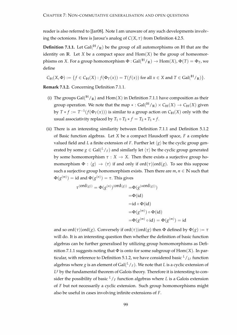
CHAPTER 7: NON-COMMUTATIVE GENERALISATION AND OPEN QUESTIONS
reader is also referred to [Jar08]. Note I am unaware of any such developments involv-
ing the octonions. Here is Jarosz’s analog of C(X, τ) from Definition 4.2.5.
Definition 7.1.1. Let Gal(H/R) be the group of all automorphisms on H that are the
identity on R. Let X be a compact space and Hom(X) be the group of homeomor-
phisms on X. For a group homomorphism Φ : Gal(H/R)→ Hom(X), Φ(T) = ΦT, we
define
CH(X, Φ) := { f ∈ CH(X) : f (ΦT(x)) = T( f (x)) for all x ∈ X and T ∈ Gal(H/R)}.
Remark 7.1.2. Concerning Definition 7.1.1.
(i) The groups Gal(H/R) and Hom(X) in Definition 7.1.1 have composition as their
group operation. We note that the map ∗ : Gal(H/R)× CH(X) → CH(X) given
by T ∗ f := T−1( f (ΦT(x))) is similar to a group action on CH(X) only with the
usual associativity replaced by T1 ◦ T2 ∗ f = T2 ∗ T1 ∗ f .
(ii) There is an interesting similarity between Definition 7.1.1 and Definition 5.1.2
of Basic function algebras. Let X be a compact Hausdorff space, F a complete
valued field and L a finite extension of F. Further let 〈g〉 be the cyclic group gen-
erated by some g ∈ Gal(L/F) and similarly let 〈τ〉 be the cyclic group generated
by some homeomorphism τ : X → X. Then there exists a surjective group ho-
momorphism Φ : 〈g〉 → 〈τ〉 if and only if ord(τ)|ord(g). To see this suppose
such a surjective group homomorphism exists. Then there are m, n ∈N such that
Φ(g(m)) = id and Φ(g(n)) = τ. This gives
τ(ord(g)) = Φ(g(n))(ord(g)) =Φ(g(nord(g)))
=Φ(id)
=id ◦Φ(id)
=Φ(g(m)) ◦Φ(id)
=Φ(g(m) ◦ id) = Φ(g(m)) = id
and so ord(τ)|ord(g). Conversely if ord(τ)|ord(g) then Φ defined by Φ(g) := τ
will do. It is an interesting question then whether the definition of basic function
algebras can be further generalised by utilizing group homomorphisms as Defi-
nition 7.1.1 suggests noting that Φ is onto for some subgroup of Hom(X). In par-
ticular, with reference to Definition 5.1.2, we have considered basic L/Lg function
algebras where g is an element of Gal(L/F). We note that L is a cyclic extension of
Lg by the fundamental theorem of Galois theory. Therefore it is interesting to con-
sider the possibility of basic L/F function algebras where L is a Galois extension
of F but not necessarily a cyclic extension. Such group homomorphisms might
also be useful in cases involving infinite extensions of F.
99

CHAPTER 7: NON-COMMUTATIVE GENERALISATION AND OPEN QUESTIONS
(iii) Turning our attention back to the non-commutative setting, as a conjecture I sug-
gests that Definition 7.1.1 may also be useful if Gal(H/R) is replaced by a sub-
group, particularly when considering extensions of the algebra.
Definition 7.1.1 has been used by Jarosz in the representation of non-commutative real
Banach algebras with square preserving norm as follows.
Definition 7.1.3. A real algebra A is fully non-commutative if every nonzero multiplica-
tive, linear functional ϕ : A→H is surjective.
Theorem 7.1.4. Let A be a non-commutative real Banach algebra with ‖a2‖A = ‖a‖2A for all
a ∈ A. Then there is a compact set X and an isomorphism Φ : Gal(H/R) → Hom(X) such
that A is isometrically isomorphic with a subalgebra A of CH(X, Φ). Furthermore a ∈ A is
invertible if and only if the corresponding element a ∈ A does not vanish on X. If A is fully
non-commutative then A = CH(X, Φ).
Jarosz also gives the following Stone-Weierstrass theorem type result.
Theorem 7.1.5. Let X be a compact Hausdorff space and let A be a fully non-commutative
closed subalgebra of CH(X). Then A = CH(X) if and only if A strongly separates the points
of X, that is for all x1, x2 ∈ X with x1 6= x2 there is f ∈ A satisfying f (x1) 6= f (x2) = 0.
7.1.2 Non-commutative non-Archimedean analogs
Non-commutative, non-Archimedean analogs of uniform algebras have yet to be seen.
Hence in this subsection we give an example of a non-commutative extension of a
complete non-Archimedean field which would be appropriate when considering such
analogs of uniform algebras. We first have the following definition from the general
theory of quaternion algebras. The main reference for this subsection is [Lam05, Ch3]
but [Lew06] is also useful.
Definition 7.1.6. Let F be a field, with characteristic not equal to 2, and s, t ∈ F× where
s = t is allowed. We define the quaternion F-algebra ( s,tF ) as follows. As a 4-dimensional
vector space over F we define(s, tF
):= {a + bi + cj + dk : a, b, c, d ∈ F}
with {1, i, j, k} as a natural basis giving the standard coordinate-wise addition and
scalar multiplication. As an F-algebra, multiplication in ( s,tF ) is given by
i2 = s, j2 = t, k2 = ij = −ji
together with the usual distributive law and multiplication in F.
100
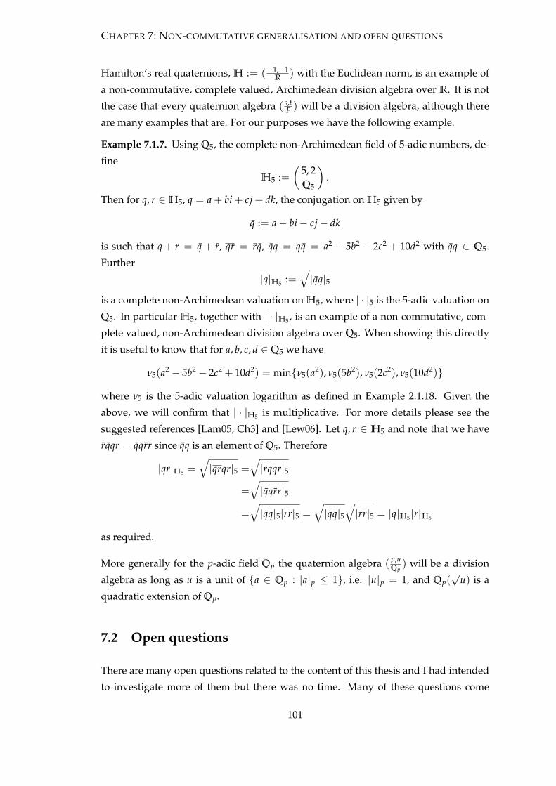
CHAPTER 7: NON-COMMUTATIVE GENERALISATION AND OPEN QUESTIONS
Hamilton’s real quaternions, H := (−1,−1R
) with the Euclidean norm, is an example of
a non-commutative, complete valued, Archimedean division algebra over R. It is not
the case that every quaternion algebra ( s,tF ) will be a division algebra, although there
are many examples that are. For our purposes we have the following example.
Example 7.1.7. Using Q5, the complete non-Archimedean field of 5-adic numbers, de-
fine
H5 :=(
5, 2Q5
).
Then for q, r ∈H5, q = a + bi + cj + dk, the conjugation on H5 given by
q := a− bi− cj− dk
is such that q + r = q + r, qr = rq, qq = qq = a2 − 5b2 − 2c2 + 10d2 with qq ∈ Q5.
Further
|q|H5 :=√|qq|5
is a complete non-Archimedean valuation on H5, where | · |5 is the 5-adic valuation on
Q5. In particular H5, together with | · |H5 , is an example of a non-commutative, com-
plete valued, non-Archimedean division algebra over Q5. When showing this directly
it is useful to know that for a, b, c, d ∈ Q5 we have
ν5(a2 − 5b2 − 2c2 + 10d2) = min{ν5(a2), ν5(5b2), ν5(2c2), ν5(10d2)}
where ν5 is the 5-adic valuation logarithm as defined in Example 2.1.18. Given the
above, we will confirm that | · |H5 is multiplicative. For more details please see the
suggested references [Lam05, Ch3] and [Lew06]. Let q, r ∈ H5 and note that we have
rqqr = qqrr since qq is an element of Q5. Therefore
|qr|H5 =√|qrqr|5 =
√|rqqr|5
=√|qqrr|5
=√|qq|5|rr|5 =
√|qq|5
√|rr|5 = |q|H5 |r|H5
as required.
More generally for the p-adic field Qp the quaternion algebra ( p,uQp
) will be a division
algebra as long as u is a unit of {a ∈ Qp : |a|p ≤ 1}, i.e. |u|p = 1, and Qp(√
u) is a
quadratic extension of Qp.
7.2 Open questions
There are many open questions related to the content of this thesis and I had intended
to investigate more of them but there was no time. Many of these questions come
101

CHAPTER 7: NON-COMMUTATIVE GENERALISATION AND OPEN QUESTIONS
from the need to generalise established Archimedean results whilst others arise from
the developing theory itself. We now consider some of these questions and note that
several of them appear to be quite accessible.
(Q1) J. Wermer gave the following theorem in 1963.
Theorem 7.2.1. Let X be a compact Hausdorff space, A ⊆ CC(X) a complex uniform
algebra and <(A) := {<( f ) : f = <( f ) + i=( f ) ∈ A} the set of the real components
of the functions in A. If <(A) is a ring then A = CC(X).
The following analog of Theorem 7.2.1 for real function algebras was given by S.
H. Kulkarni and N. Srinivasan in [KS90], although I have not used their notation.
Theorem 7.2.2. Let X be a compact Hausdorff space, τ a topological involution on X
and A a C/R function algebra on (X, τ, z), i.e. a real function algebra. If <(A) is a ring
then A = C(X, τ, z).
It is interesting to know whether Theorem 7.2.2 can be generalised to all L/Lg
function algebras on (X, τ, g). Of course the result would be trivial if, in the non-
Archimedean setting, the basic L/Lg function algebra on (X, τ, g) is the only L/Lg
function algebra on (X, τ, g). With analogy to <(A) above, in this case we should
ask whether the set of Lg components of the functions in C(X, τ, g) form a ring.
(Q2) As alluded to in (Q1) we have not given an example in the non-Archimedean
setting of a L/Lg function algebra on (X, τ, g) that is not basic. We need to know
whether the basic function algebras are the only such examples. Theorem 4.2.3,
Kaplansky’s version of the Stone Weierstrass Theorem, may be important here.
Further even if in the non-Archimedean setting there is a L/Lg function algebra on
(X, τ, g) that is not basic, such an algebra might still be isometrically isomorphic
to some Basic function algebras.
(Q3) With reference to Theorem 6.2.9 we note that there are plenty of examples of
commutative, unital Banach F-algebras with finite basic dimension in the non-
Archimedean setting. Indeed if K is not only a finite Galois extension of F but
also a cyclic extension then taking A := K gives such an algebra. In this case
the character spaceM(A) will be finite with each element given by an element
of Gal(K/F), see the proof of Theorem 6.2.9 for details. However such examples
are not particularly interesting and it would be good to know whether all L/Lg
function algebras on (X, τ, g) have finite basic dimension so that Theorem 6.2.9
becomes closer to a characterisation result. We recall that all commutative uni-
tal complex Banach algebras and commutative unital real Banach algebras have
finite basic dimension, see Remark 6.2.10.
102

CHAPTER 7: NON-COMMUTATIVE GENERALISATION AND OPEN QUESTIONS
(Q4) With reference to Definition 5.1.2 of the basic L/Lg function algebra on (X, τ, g)
the map σ( f ) = g(ord(g)−1) ◦ f ◦ τ on CL(X) is such that each f ∈ CL(X) is an
element of C(X, τ, g) if and only if σ( f ) = f . We have seen that σ is either an
algebraic involution on CL(X) or a algebraic element of finite order on CL(X). It
should be established whether every such involution and element of finite order
on CL(X) has the form of σ for some g and τ. This is the case for real function
algebras, see [KL92, p29].
(Q5) As described in Remark 7.1.2 it might be possible to generalise the definition of
Basic function algebras by involving a group homomorphism in the definition.
The algebras currently given by Definition 5.1.2 could then appropriately be re-
ferred to as cyclic basic function algebras given that the group Gal(L/Lg) is cyclic.
Further the possibility of generalising the definition of Basic function algebras to
the case where the functions take values in some infinite extension of the under-
lying field over which the algebra is a vector space should also be considered.
The involvement of a group homomorphism might also be useful in this case as
well as some more of the theory from [Ber90].
(Q6) As seen in Subsection 7.1.2 the general theory of quaternion algebras provides the
necessary structures for generalising the theory of non-commutative real function
algebras to the non-Archimedean setting. Further with reference to Subsection
5.4.1 it would be interesting to see what sort of lattice of basic extensions the
non-commutative real function algebras have. We can also look at this in the
non-Archimedean setting along with the residue algebra.
(Q7) A proof of the following theorem can be found in [KL92, p18].
Theorem 7.2.3. Let A be a unital Banach algebra in the Archimedean setting satisfying
one of the following conditions:
(i) the algebra A is a complex algebra and there exists some positive constant c such
that ‖a‖2A ≤ c‖a2‖A for all a ∈ A;
(ii) the algebra A is a real algebra and there exists some positive constant c such that
‖a‖2A ≤ c‖a2 + b2‖A for all a, b ∈ A with ab = ba.
Then A is commutative.
It would be interesting to establish whether there is such a theorem for all unital
Banach F-algebras. If not then perhaps some special cases are possible in the
non-Archimedean setting. The proof of theorem 7.2.3 uses Liouville’s theorem
and some spectral theory in the Archimedean setting. Both of these are different
in the non-Archimedean setting, see Theorem 3.1.9 and Subsection 3.2.1.
103

CHAPTER 7: NON-COMMUTATIVE GENERALISATION AND OPEN QUESTIONS
(Q8) It might be interesting to investigate the isomorphism classes of basic function
algebras. That is for a given basic function algebra A are there other basic function
algebras that are isometrically isomorphic to A.
(Q9) It is interesting to consider whether the Kaplansky spectrum of Remark 3.2.13 can
be used for some cases in the non-Archimedean setting and, if so, whether it is
one such definition in some larger family of definitions of spectrum applicable in
the non-Archimedean setting.
(Q10) More broadly the established theory of Banach algebras provides a large supply
of topics that can be considered for generalisation over complete valued fields. In
addition to several of the other references included in this thesis [Dal00] will be
of much interest when considering such possibilities. One obvious example is the
generalisation of automatic continuity results. That is what conditions on a Ba-
nach F-algebra force homomorphisms from, or to, that algebra to be continuous.
There is one such result in this thesis noting that in Theorem 6.2.9 the elements
ofM(A) are automatically continuous. Further [BBN73] may also be of interest
concerning function algebras.
(Q11) As mentioned in Remark 4.1.20 there is a possible generalisation of the Swiss
cheese classicalisation theorem to the Riemann sphere and possibly to a more
general class of metric spaces.
(Q12) It might be interesting to consider generalising over all complete valued fields
the theory of algebraic extensions of commutative unital normed algebras. See
the survey paper [Daw03] for details.
(Q13) The possibility of generalising C∗-Algebras over complete valued fields is inter-
esting but perhaps not straightforward. The Levi-Civita field might be of interest
here since it is totally ordered such that the order topology agrees with the val-
uation topology. Hence it might be possible to define positive elements in this
case. Perhaps the algebraic elements of finite order mentioned in (Q4) are rele-
vant. Also there is a monograph by Goodearl from 1982 that considers real C∗-
Algebras that might be of use. The possibility of a non-Archimedean theory of
Von Neumann algebras might also be a good place to start.
104
References
[AJ04] Mati Abel and Krzysztof Jarosz. Noncommutative uniform algebras. Studia
Math., 162(3):213–218, 2004.
[Apo74] Tom M. Apostol. Mathematical analysis. Addison-Wesley Publishing Co.,
Reading, Mass.-London-Don Mills, Ont., second edition, 1974.
[BBN73] G. Bachman, E. Beckenstein, and L. Narici. Function algebras over valued
fields. Pacific J. Math., 44:45–58, 1973.
[Ber90] Vladimir G. Berkovich. Spectral theory and analytic geometry over non-
Archimedean fields, volume 33 of Mathematical Surveys and Monographs. Amer-
ican Mathematical Society, Providence, RI, 1990.
[Bro69] Andrew Browder. Introduction to function algebras. W. A. Benjamin, Inc., New
York-Amsterdam, 1969.
[Dal00] H. G. Dales. Banach algebras and automatic continuity, volume 24 of London
Mathematical Society Monographs. New Series. The Clarendon Press Oxford
University Press, New York, 2000. Oxford Science Publications.
[Daw03] Thomas Dawson. A survey of algebraic extensions of commutative, unital
normed algebras. In Function spaces (Edwardsville, IL, 2002), volume 328 of
Contemp. Math., pages 157–170. Amer. Math. Soc., Providence, RI, 2003.
[Esc03] Alain Escassut. Ultrametric Banach algebras. World Scientific Publishing Co.
Inc., River Edge, NJ, 2003.
[Fei04] J. F. Feinstein. A counterexample to a conjecture of S. E. Morris. Proc. Amer.
Math. Soc., 132(8):2389–2397 (electronic), 2004.
[FH10] J. F. Feinstein and M. J. Heath. Swiss cheeses, rational approximation and
universal plane curves. Studia Math., 196(3):289–306, 2010.
[FV02] I. B. Fesenko and S. V. Vostokov. Local fields and their extensions, volume 121
of Translations of Mathematical Monographs. American Mathematical Society,
Providence, RI, second edition, 2002. With a foreword by I. R. Shafarevich.
105

REFERENCES
[Gam69] Theodore W. Gamelin. Uniform algebras. Prentice-Hall Inc., Englewood Cliffs,
N. J., 1969.
[Hea08] M. J. Heath. Bounded derivations from Banach algebras. Ph.d. thesis, University
of Nottingham, February 2008.
[Jar08] Krzysztof Jarosz. Function representation of a noncommutative uniform al-
gebra. Proc. Amer. Math. Soc., 136(2):605–611 (electronic), 2008.
[Kap50] Irving Kaplansky. The Weierstrass theorem in fields with valuations. Proc.
Amer. Math. Soc., 1:356–357, 1950.
[Kel75] John L. Kelley. General topology. Springer-Verlag, New York, 1975. Reprint of
the 1955 edition [Van Nostrand, Toronto, Ont.], Graduate Texts in Mathemat-
ics, No. 27.
[KL81] S. H. Kulkarni and B. V. Limaye. Gleason parts of real function algebras.
Canad. J. Math., 33(1):181–200, 1981.
[KL92] S. H. Kulkarni and B. V. Limaye. Real function algebras, volume 168 of Mono-
graphs and Textbooks in Pure and Applied Mathematics. Marcel Dekker Inc., New
York, 1992.
[KS90] S. H. Kulkarni and N. Srinivasan. An analogue of Wermer’s theorem for a
real function algebra. Math. Today, 8:33–42, 1990.
[Lam05] T. Y. Lam. Introduction to quadratic forms over fields, volume 67 of Graduate
Studies in Mathematics. American Mathematical Society, Providence, RI, 2005.
[Lew06] David W. Lewis. Quaternion algebras and the algebraic legacy of Hamilton’s
quaternions. Irish Math. Soc. Bull., (57):41–64, 2006.
[Mas10] J. W. D. Mason. An inductive proof of the Feinstein-Heath Swiss cheese “clas-
sicalisation” theorem. Proc. Amer. Math. Soc., 138(12):4423–4432, 2010.
[Mas11] J. W. D. Mason. A survey of non-complex analogs of uniform algebras. In
Function spaces, volume 547 of Contemp. Math. Amer. Math. Soc., Providence,
RI, 2011.
[McC66] Paul J. McCarthy. Algebraic extensions of fields. Blaisdell Publishing Co. Ginn
and Co. Waltham, Mass.-Toronto, Ont.-London, 1966.
[Roq84] Peter Roquette. Some tendencies in contemporary algebra. In Perspectives in
mathematics, pages 393–422. Birkhäuser, Basel, 1984.
106

REFERENCES
[Rot38] Alice Roth. Approximationseigenschaften und Strahlengrenzwerte mero-
morpher und ganzer Funktionen. Comment. Math. Helv., 11(1):77–125, 1938.
[Rud87] Walter Rudin. Real and complex analysis. McGraw-Hill Book Co., New York,
third edition, 1987.
[SB10] Khodr Shamseddine and Martin Berz. Analysis on the Levi-Civita field, a
brief overview. In Advances in p-adic and non-Archimedean analysis, volume
508 of Contemp. Math., pages 215–237. Amer. Math. Soc., Providence, RI, 2010.
[Sch02] Peter Schneider. Nonarchimedean functional analysis. Springer Monographs in
Mathematics. Springer-Verlag, Berlin, 2002.
[Sch06] W. H. Schikhof. Ultrametric calculus, volume 4 of Cambridge Studies in Ad-
vanced Mathematics. Cambridge University Press, Cambridge, 2006. An intro-
duction to p-adic analysis, Reprint of the 1984 original [MR0791759].
[Sha00] Daniel B. Shapiro. Compositions of quadratic forms, volume 33 of de Gruyter
Expositions in Mathematics. Walter de Gruyter & Co., Berlin, 2000.
[Sto71] Edgar Lee Stout. The theory of uniform algebras. Bogden & Quigley, Inc.,
Tarrytown-on-Hudson, N. Y., 1971.
[Wil04] Stephen Willard. General topology. Dover Publications Inc., Mineola, NY, 2004.
Reprint of the 1970 original [Addison-Wesley, Reading, MA; MR0264581].
[Zha93] Guan Hou Zhang. Theory of entire and meromorphic functions, volume 122
of Translations of Mathematical Monographs. American Mathematical Society,
Providence, RI, 1993. Deficient and asymptotic values and singular direc-
tions, Translated from the Chinese by Chung-chun Yang.
107


