Mass Transfer Boundary Layer Theory Transfer – Boundary Layer Theory 9-3 In addition to this,...

Boundary Layer Theory: Mass and Heat/Momentum Transfer

Mass Transfer

Lecture 10, 22.11.2017, Dr. K. Wegner

Mass Transfer – Boundary Layer Theory 9-2

9.1 Fluid-Fluid Interfaces (lecture of 15.11.17)

9. Basic Theories for Mass Transfer Coefficients

9.2 Fluid-Solid Interfaces

Fluid-fluid interfaces are typically not fixed and are strongly affected by the flow leading to heterogeneous systems that make it difficult to development a general theory behind the MT correlations (Cussler Table 8.3-2).

Solids typically have fixed and well-defined surfaces, allowing to develop theoretical foundations for the empirical MT correlations (Cussler Table 8.3-3). In contrast to fluid-fluid interfaces the models are far more rigorous but, unfortunately, computationally INTENSIVE.


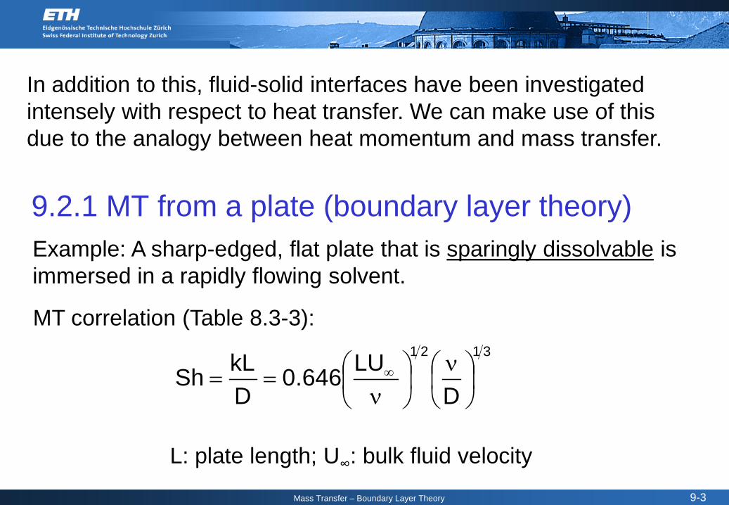
In addition to this, fluid-solid interfaces have been investigated intensely with respect to heat transfer. We can make use of this due to the analogy between heat momentum and mass transfer.

9.2.1 MT from a plate (boundary layer theory)

MT correlation (Table 8.3-3):3121

DLU646.0

DkLSh

ν

ν== ∞

Example: A sharp-edged, flat plate that is sparingly dissolvable is immersed in a rapidly flowing solvent.

L: plate length; U∞: bulk fluid velocity


Prandtl first introduced the concept of boundary layers.

Goal: Calculate the MTC for this fluid–solid interface

Literature:R.B. Bird, W.E. Steward, E.N. Lightfoot, “Transport Phenomena”, 2nd ed. J. Wiley&Sons 2011.H. Schlichting, K. Gersten, "Boundary Layer Theory", 8th ed., Springer 1999.

x

y

The transition from zero velocity at the plate to the velocity of the surrounding free stream takes place in the boundary layer.


1. Calculate the velocity profile in the B.L.

2. Calculate the concentration profile in the B.L.

y 0cj D |y =

∂= −

∂

and set it equal to k∆c to obtain k.

3. Calculate the flux at the interface

x

y

Procedure:


The relative magnitude of the fluid flow (momentum) B.L. and the concentration B.L. is given by

kinematic viscosityScD diffusivityν

= =

Sc > 1: Momentum B.L. > Concentration B.L. (typical)

Sc = 1: Momentum B.L. = Concentration B.L.

Sc < 1: Momentum B.L. < Concentration B.L. (rare case)


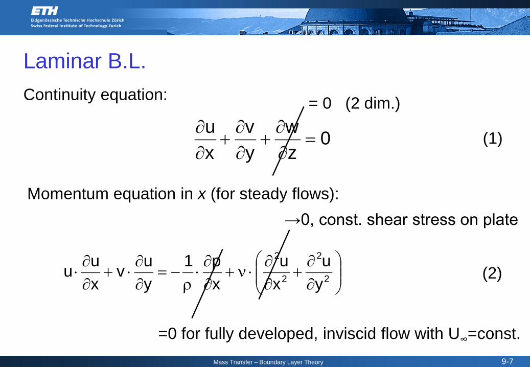
Laminar B.L.Continuity equation:

(1)

Momentum equation in x (for steady flows):

0zw

yv

xu

=∂∂

+∂∂

+∂∂

= 0 (2 dim.)

∂∂

+∂∂

⋅ν+∂∂⋅

ρ−=

∂∂⋅+

∂∂⋅ 2

2

2

2

yu

xu

xp1

yuv

xuu

→0, const. shear stress on plate

(2)

=0 for fully developed, inviscid flow with U∞=const.


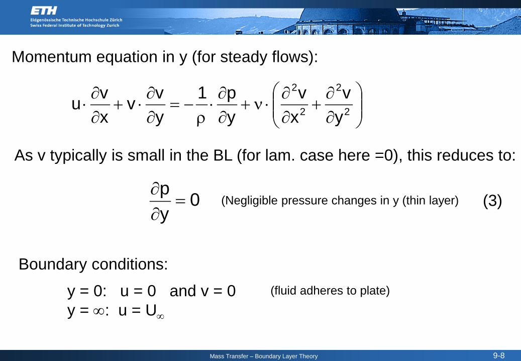
(Negligible pressure changes in y (thin layer)

y = 0: u = 0 and v = 0 y = ∞: u = U∞

Momentum equation in y (for steady flows):

∂∂

+∂∂

⋅ν+∂∂⋅

ρ−=

∂∂⋅+

∂∂⋅ 2

2

2

2

yv

xv

yp1

yvv

xvu

As v typically is small in the BL (for lam. case here =0), this reduces to:

0yp=

∂∂

(3)

Boundary conditions:(fluid adheres to plate)


Digression: How did Prandtl come up with that?

The B.L. thickness, δ, is related to Re by

Equations (1) and (2) are solved by introducing the variable

∞

⋅ν=η

Ux

y

xURe~

x21

⋅ν

=δ

∞

−

η=⋅ν

=δ

∞Ux

yRexy~y 21


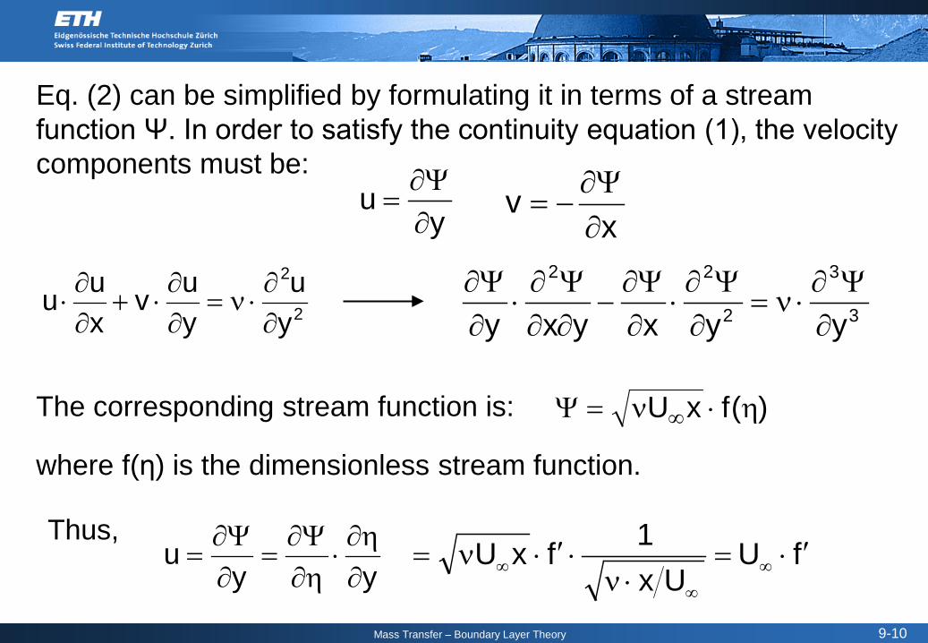
The corresponding stream function is: )(fxU η⋅ν=Ψ ∞

Eq. (2) can be simplified by formulating it in terms of a stream function Ψ. In order to satisfy the continuity equation (1), the velocity components must be:

yu

∂Ψ∂

=x

v∂Ψ∂

−=

2

2

yu

yuv

xuu

∂∂⋅ν=

∂∂⋅+

∂∂⋅ 3

3

2

22

yyxyxy ∂Ψ∂

⋅ν=∂Ψ∂

⋅∂Ψ∂

−∂∂Ψ∂

⋅∂Ψ∂

Thus,

where f(η) is the dimensionless stream function.

yyu

∂η∂

⋅η∂Ψ∂

=∂Ψ∂

= fUUx

1fxU ′⋅=⋅ν

⋅′⋅ν= ∞∞

∞


1 2 1 21 12 2

U Uν f fx x∞ ∞ν ν ′= − + η⋅

fx

U21f

Ux

yU21

xu

3′′⋅η−=′′⋅

ν−=

∂∂ ∞

∞

∞

fx

UUyu 21

′′

ν

=∂∂ ∞

∞ fx

Uyu 2

2

2′′′⋅

ν

=∂∂ ∞

1 2

1 23

1 12 2

U yν f U x fx x x

U

∞∞

∞

ν∂Ψ ′= − = − + ν ⋅ ⋅ ∂ ν ⋅

and

( )ffxU

21 21

−′⋅η

ν= ∞


Now the equation of motion (2) becomes:

0fff2 =⋅′′+′′′

at η = 0: f = 0 and f’ = 0η = ∞: f’ = 1 (see Table)

Blasius obtained the solution in the form of a series expansion at η=0 and η → ∞ (“Blasius series”) and the two forms are matched at a suitable η. See attached Table from H. Schlichting (“Boundary Layer Theory”), which gives the complete values of u and v for every x and y. The velocity profiles have been calculated.


Source: H. Schlichting, “Boundary Layer Theory”


Blasius similarity solution of the velocity distribution in a laminar boundary layer on a flat plate.P.K. Kundu, I.M. Cohen, “Fluid Mechanics” 2nd ed. 2002, Academic Press

∞Uu

xUyν

=η ∞


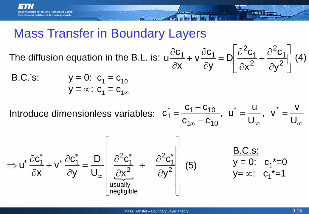
Mass Transfer in Boundary Layers

The diffusion equation in the B.L. is:

∂∂

+∂∂

=∂∂

+∂∂

21

2

21

211

yc

xcD

ycv

xcu

B.C.’s: y = 0: c1 = c10y = ∞: c1 = c1∞

Introduce dimensionless variables:∞∞∞

==−−

=Uvv,

Uuu,

ccccc **

101

101*1

∂∂

+∂∂

=∂∂

+∂∂

⇒∗∗

∞

∗∗

∗∗

21

2

negligibleusually

21

211

yc

xc

UD

ycv

xcu

B.C.s:y = 0: c1*=0y= ∞: c1*=1

(4)

(5)


Compare to the momentum equation (2):

∂

∂+

∂

∂ν=

∂∂

+∂∂ ∗∗

∞

∗∗

∗∗

2

2

negligibleusually

2

2

yu

xu

Uyu

vxu

u B.C.’s: y = 0: u*=0 and v*=0y= ∞: u*=1

The two equations have the same form!

Sc = 1: In this special case where ∞∞

=ν

UD

U

the solution to the concentration profile is given by c1*=u*

or ν = D

The boundary layers for flow and concentration are the same.


For this case we write Fick’s first law 0y1 |

ycDj =∂∂⋅−=

( )1010y

1 ccycDj −∂∂⋅−= ∞

=

∗

( ) ( )1010y

1010y

ccyu

Ucc

yu

j −∂∂ν

−=−∂∂⋅ν−= ∞

=∞∞

=

∗

( )1010

2

221

ccfx

UUU

j −

η∂∂

ν

ν−= ∞

=η

∞∞

∞

( )101Tablefromf

21

cc332.0xUj −⋅⋅

ν−= ∞

′′

∞

with c1*:


As j = k (c10 - c1∞)21

xU332.0k

ν⋅= ∞

21

xU

Dx332.0

DxkSh

⋅ν⋅⋅

νν⋅=

⋅= ∞

2121

ReSc332.0xUD

332.0 ⋅⋅=

ν⋅

ν⋅= ∞

Here, Sc = 1: 21Re332.0Sh ⋅=

This is the Local Mass Transfer Coefficient to be distinguished from the average MTC over a plate of length L (Cussler Table 8.3-3):

3121 ScRe646.0Sh ⋅⋅=

,


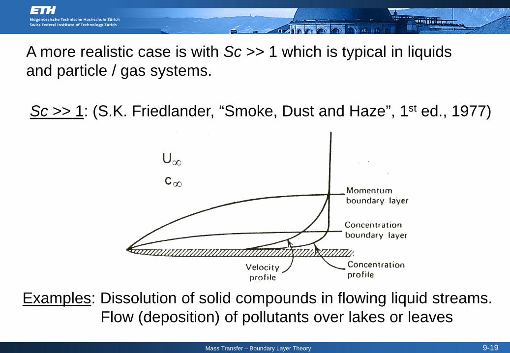
A more realistic case is with Sc >> 1 which is typical in liquids and particle / gas systems.

Sc >> 1: (S.K. Friedlander, “Smoke, Dust and Haze”, 1st ed., 1977)

Examples: Dissolution of solid compounds in flowing liquid streams.Flow (deposition) of pollutants over lakes or leaves


More specifically, if the B.L. (displacement) thickness is:1/2

x* 1.72U∞

= ⋅

νδ

For a wind blowing at a speed of 10 km/h, δ ≈ 0.5 mm. E.g., at 2 cm from the leading edge of the flat surface:

Goal: To obtain the mass transfer coefficient

mm56.0m1033.072.13600sm10000

mkg1s Pa1015m02.0

72.1 33

6

* =⋅⋅=

⋅⋅⋅=δ −

−

(Blasius, Schlichting)


Again at steady-state 2

*1

2*1*

*1*

yc

UD

ycv

xcu

∂∂

=∂∂

+∂∂

∞

Expand and

near the wall (η→0) into Taylor series:

( )η′==∞

fUuu* ( ))(f)(f

xU21

Uvv

21* η−η′⋅η

ν==

∞∞

η=η+≈+η⋅′′′+η⋅′′+′=

∞

= a332.00...2

)0(f)0(f)0(fUuu

2*

disregard higher order terms

221

221

3221

*

xU4a

2332.00

xU21

...)0(f31)0(f

21)0(f

xU21

Uvv

η

ν=

η+

ν≈

+η′′′+η′′+

ν==

∞∞

∞∞

(5)


Substitution in the above differential equation (5) gives:

Assume that c1* is a fct only of η: )(gc*1 η=

Then:

gx2

1xc*

1 ′⋅η

−=∂∂

2

*1

2*12

21*1

yc

UD

yc

Ux4a

xca

∂∂

=∂∂

η

⋅ν

+∂∂

η∞∞

gx

Uy

gyc 21*

1 ′⋅

ν

=∂η∂

η∂∂

=∂∂ ∞

gx

Uyc2

*1

2

′′⋅

ν

=∂∂ ∞

ν∞ ⋅

1/2Uη = yx

with


Introducing the above variables in the diffusion equation:

or∞=η

=η 01g0g

==

Solution: Set

00

gP=η

η∂∂

=where

gx

UUDg

xU

Ux4ag

x2a

212

212

′′ν

=′

ν

η

⋅ν

+

′η

− ∞

∞

∞

∞

0gD4

ag 2 =′⋅η⋅

ν+′′ with

0PSc4aP gP 2 =⋅⋅η+

η∂∂

⇒′=

Integrate: Sc12a

PPln 3

0

⋅η−=


From the B.C’s.: at η = 0, g = 0:

From the B.C’s.: at η = ∞, g = 1, hence:

η−⋅==

η∂∂ Sc

12aexpPPg 3

0

dr rSc12aexpPg

0

30 ∫η

⋅−=

1

0m

30 dr rSc

12aexpP

−

∞

⋅−= ∫


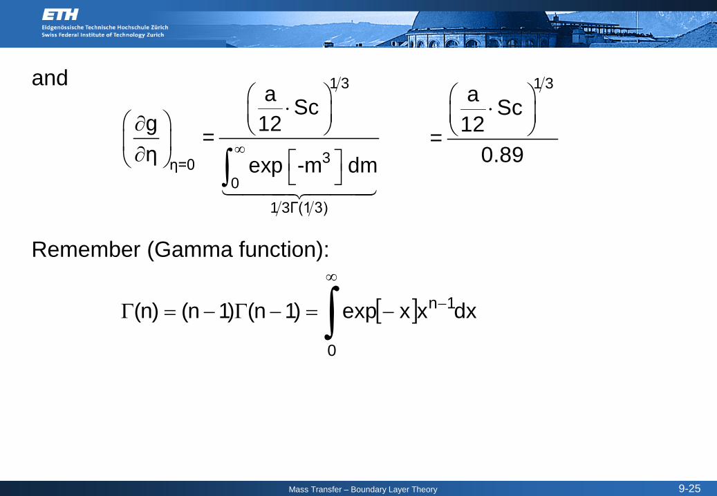
and

∞

⋅ ∂ ∂

∫

1 3

3η=00

1 3Γ(1 3)

a Scg 12=η exp -m dm

⋅

1 3a Sc12=

0.89

Remember (Gamma function):

[ ]∫∞

−−=−Γ−=Γ

0

1n dxxxexp)1n()1n()n(


( )0 ∞

∂⋅ ⋅ ∂

*1

1 1y=0

c= D c - cy

( )ν∞

∞ ∂ ⋅ ⋅ ∂

1 2

10 1η=0

U g= D c - cx η

( )νν

∞∞

∞

1 2 1 3

10 1UD a= Sc c - c

U x 0.89 12

( )∞∞

⋅ ⋅

1 3-2 3 -1 2

10 1

k

U 0.332= Sc Re c - c0.89 12

0y

1

ycDj

=∂∂⋅−=


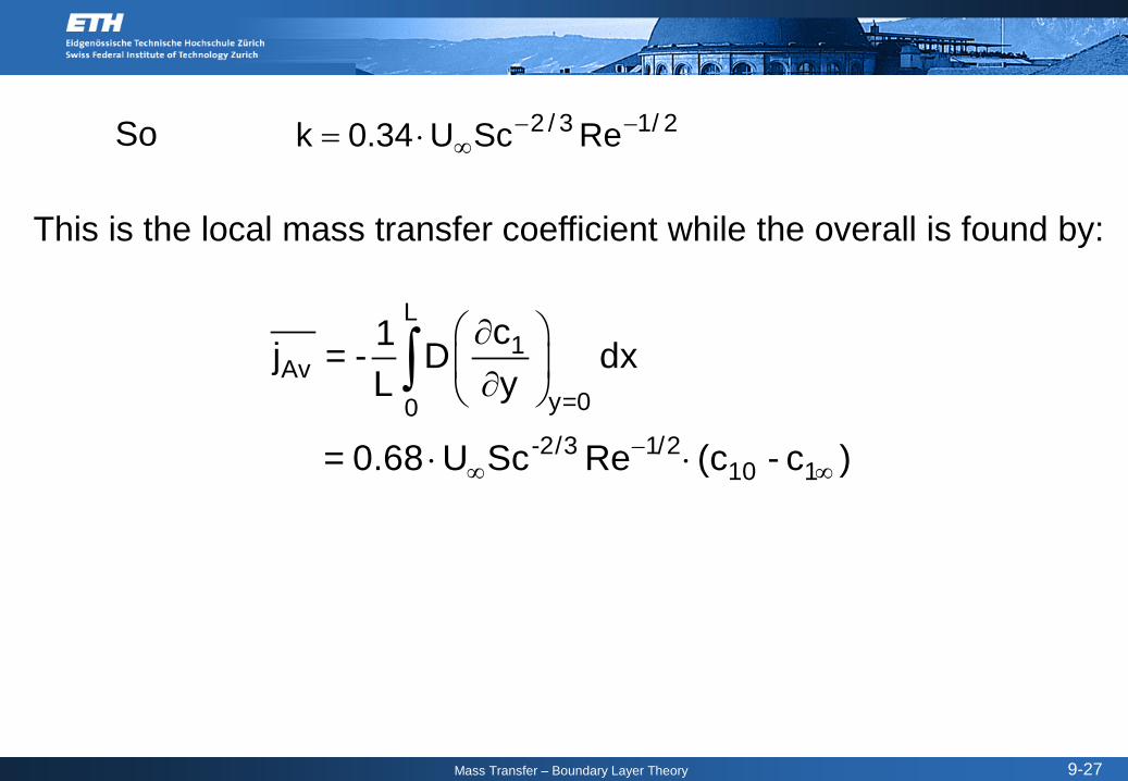
2/13/2 ReScU34.0k −−∞⋅=So

This is the local mass transfer coefficient while the overall is found by:

L1

Avy=00

-2/3 1/210 1

c1j = - D dxL y

= 0.68 U Sc Re (c - c )−∞ ∞

∂ ∂

⋅ ⋅

∫


Let’s calculate Sh to compare it with our Table of correlations

2/3 1/2

2/3 1/2

2/3 1/2 1/2

1/3 1/2

1/3 1/2

kL L0.68 Sc Re UD D

L D0.68 uD u L

uL0.68D

0.68 Sc Re

− −∞=

ν=

ν

ν = ν

= ⋅

So we obtained the mass transfer coefficient from theory!


In general 2/13/2 ReScconstUk

cUj −−

∞∞⋅==

∆

Applicable for flow around spheres, cylinders etc.

Mass transfer correlation over a wide range of Re:

3/12/1 ScRe6.02Sh +=


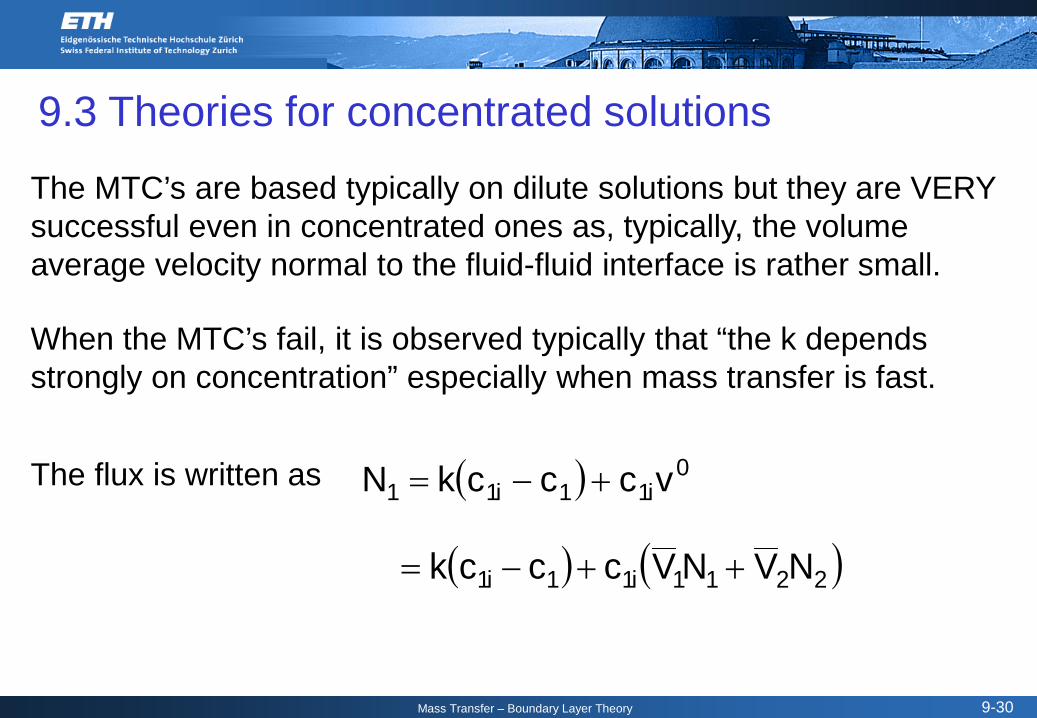
9.3 Theories for concentrated solutions

The MTC’s are based typically on dilute solutions but they are VERY successful even in concentrated ones as, typically, the volume average velocity normal to the fluid-fluid interface is rather small.

When the MTC’s fail, it is observed typically that “the k depends strongly on concentration” especially when mass transfer is fast.

The flux is written as ( ) 0i11i11 vccckN +−=

( ) ( )2211i11i1 NVNVccck ++−=


However, this is difficult and we also have the previous unknowns again (film thickness, contact or residence times).Instead we are looking for corrections to the dilute mass transfer coefficient by the film theory:

0k MTC in concentrated solution=

MTC in dilute solutionk

This framework can be used to build new film, penetration and surface-renewal theories.


The total flux for a concentrated solution across a film:

01

11 vc

dzdcDn +−= with B.C.’s: z = 0: c1 = c1i

z = L c1 = c1

For concentrated solutions, n1 and v0 are constant, so the above equation can be integrated from z=0 to L to give

[ ]D/Lvexpv/ncv/nc 0

01i1

011 ⋅=

−−

Rearranging:

Compare: ( ) 0i11i11 vccckN +−=

[ ] ( ) 0i11i10

0

10z1 vccc1D/Lvexp

vNn +−−⋅

===


Then the mass transfer coefficient is

[ ] 1D/Lvexpvk 0

0

−⋅=

For dilute solutions:LDk0 =

Taking the ratio k/k0, we eliminate the dependency in L:

[ ] 1k/vexpk/v

kk

00

00

0 −=


k can be smaller or larger than k0

depending on the direction of v0.

1ekv

kk

00 kv

00

0 −=

00 kv

00 kv

0kk

Flux awayfrom interphase

Flux towardinterphase

Source:Bird, Stewart, Lightfoot, "Transport Phenomena"

Date post:	01-May-2018
Category:	Documents
Upload:	vudat
View:	218 times
Download:	4 times

Mass Transfer Boundary Layer Theory Transfer – Boundary Layer Theory 9-3 In addition to this,...

Documents