Massachusetts Institute of Technology, École Normale Supérieure Geometrically induced rigidity of thin shells & Negative Poisson’s ratio structures First year Master’s Degree research internship Claude Perdigou [email protected]Under the supervision of Pr. Pedro Reis February, 8th - July, 31st 2010
Transcript
Massachusetts Institute of Technology,École Normale Supérieure
AbstractThis report presents new experimental and theoretical results on the mechanics of
thin shells. In the first part we will focus on thin shells of revolution and geometricallyinduced rigidity. The theory of spherical thin shells will be extended to axisymmetric el-lipsoids. Experiments explore the linear and nonlinear regime for plate and point load onthin shells of revolution. In the linear regime we compare the effective Young’s moduluswith theoretical predictions. In the nonlinear regime, we will study buckling and stresslocalization.
The second part of this report features recent advancements in the creation of a sim-ple three dimensional structure showing a negative Poisson’s ratio. Although the structurecreated does not show an auxetic behavior under uniaxial compression, we bring to lighta mechanical instability that occurs when uniform pressure is applied.
Keywords : mechanics of thin structures, geometrically induced rigidity, theory ofthin shells, stress localization, mechanical instability, negative Poisson’s ratio.
RésuméCe rapport de stage présente des résultats nouveaux en mécanique des structures
fines. La première partie se concentre sur les coquilles fines de révolution, et en particuliersur l’influence de la géométrie sur les propriétés mécaniques de ces objets. Des résultatsexpérimentaux et théoriques sont présentés. D’un point de vue théorique, on étend unethéorie déjà existante pour les coquilles sphériques au cas des coquilles ellipsoïdes. Ex-périmentalement, on compare le régime linéaire aux prédictions théoriques, et on étudiele régime non linéaire ; en particulier le cas du flambage et de la localisation de la con-trainte.
La seconde partie de ce texte expose des progrès récents dans la création d’unestructure tri-dimensionnelle présentant un nombre de Poisson négatif. Bien que la struc-ture obtenue ne présente pas ce comportement lors d’une compression axiale, on met enévidence une instabilité mécanique lorsqu’une pression est appliquée uniformément.
Mots-clés : mécanique des structures fines, influence de la géométrie sur les pro-priétés mécaniques, théorie des coquilles fines, localisation de la contrainte, instabilitémécanique, nombre de Poisson négatif.
IntroductionMy internship took place at the Massachusetts Institute of Technology in Cam-
bridge, USA. From early February to the end of July, I worked with Professor Pedro Reisin the departments of Mechanical Engineering and Civil and Environmental Engineering.I also had the opportunity to work with Professor Katia Bertoldi from the School of En-gineering and Applied Science of Harvard University, also in Cambridge.
During my internship I worked in the EGSLab (Elasticity, Geometry and StatisticsLaboratory) and the most important results I obtained while experimenting on thin shellsare detailed in the first part of this report. My work is concerned with the mechanicalproperties of thin shells, in the linear and nonlinear regimes. I studied both the exper-imental and theoretical aspects, all of which are reviewed in this first chapter. Someimportant experimental technicalities and secondary results I studied during my intern-ship can be found in appendix.
The second chapter of this report is dedicated to a secondary project that startedas soon as I arrived. A joint project between my advisor Pedro Reis and his friend KatiaBertoldi regarding structures with a negative Poisson ratio was already on the agenda atthe time of my arrival. Seeing my interest in the project, they offered me to take part init. The main idea was to create a three dimensional structure showing a negative Poissonratio. This technical notion, along with the results obtained while working on this projectare detailed in the second chapter of this report.
Most of the work I have done is on the mechanics of thin shells, but my secondaryproject took more and more importance towards the end of my internship. For that rea-son, an important part of my report is dedicated to it.
3
Chapter 1
Geometrically induced rigidity of thinshells
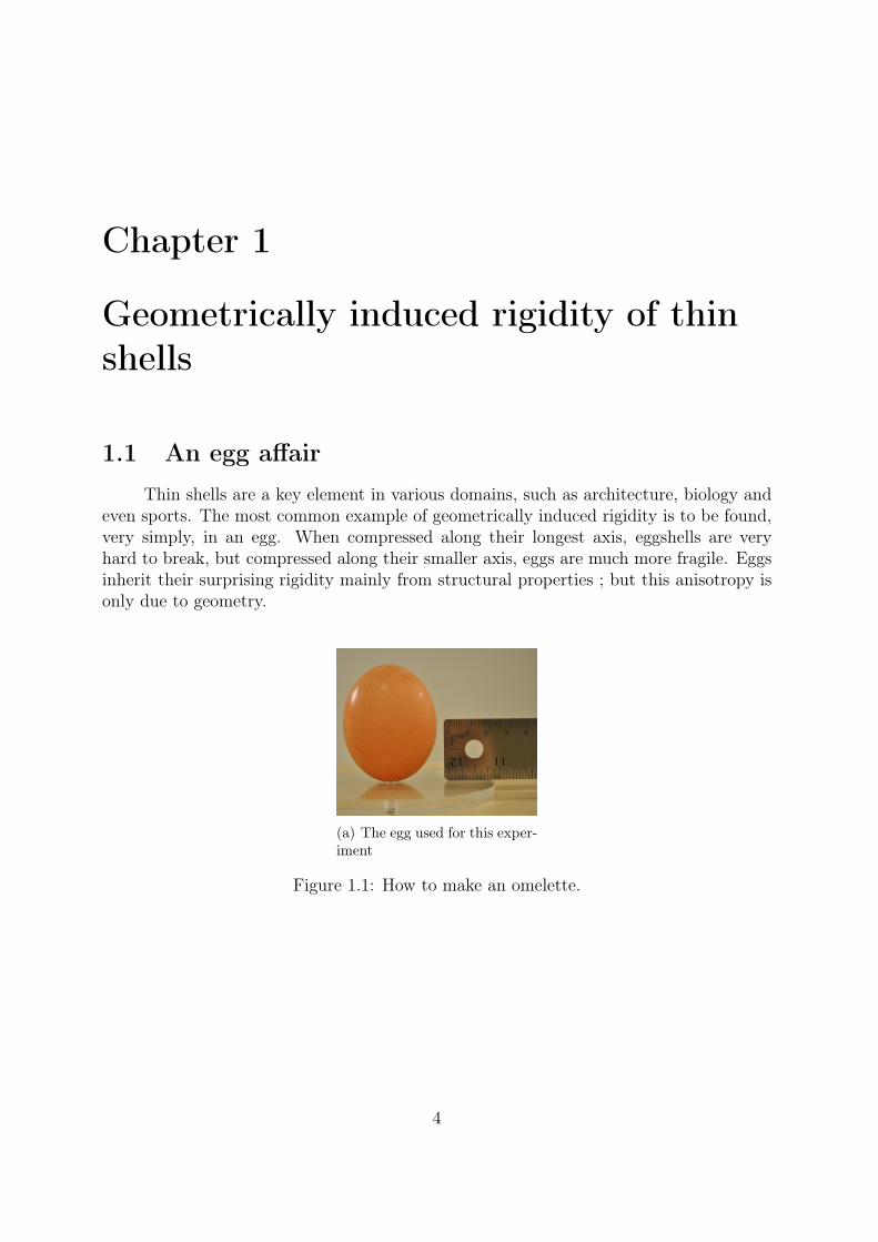
1.1 An egg affairThin shells are a key element in various domains, such as architecture, biology and
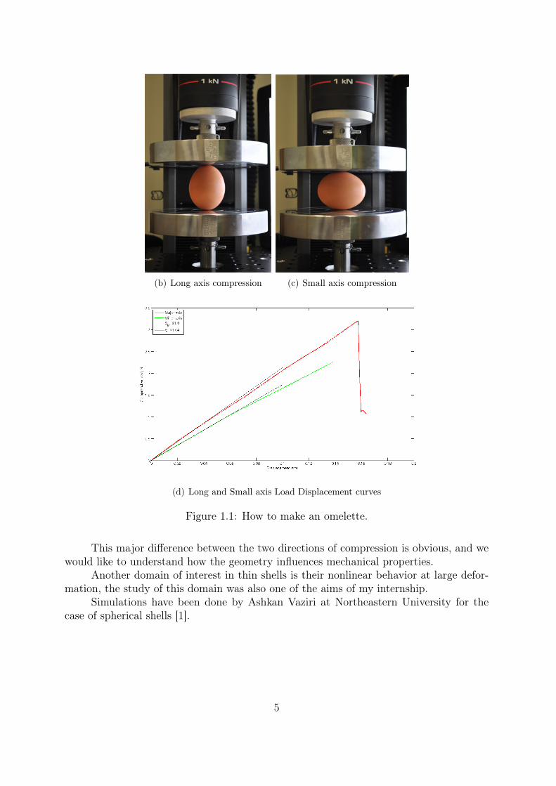
even sports. The most common example of geometrically induced rigidity is to be found,very simply, in an egg. When compressed along their longest axis, eggshells are veryhard to break, but compressed along their smaller axis, eggs are much more fragile. Eggsinherit their surprising rigidity mainly from structural properties ; but this anisotropy isonly due to geometry.
(a) The egg used for this exper-iment
Figure 1.1: How to make an omelette.
4
(b) Long axis compression (c) Small axis compression
(d) Long and Small axis Load Displacement curves
Figure 1.1: How to make an omelette.
This major difference between the two directions of compression is obvious, and wewould like to understand how the geometry influences mechanical properties.
Another domain of interest in thin shells is their nonlinear behavior at large defor-mation, the study of this domain was also one of the aims of my internship.
Simulations have been done by Ashkan Vaziri at Northeastern University for thecase of spherical shells [1].
5
1.2 The birth of a shellUpon my arrival at the MIT, the lab I was to work was not ready yet, so that I had
time to work on theoretical and computer-related problems. Of course, I helped to set upthe lab, but even before that, my very first task was to install the various software thatmight be needed for future work.
Regarding the creation of our shells, many options seemed possible. We could eitherprint them directly with a 3D printer, order them online from a specialized company, orcast them in molds that had to be created.
All these methods implied one thing : having a .STL file (basic exchange format for3D designs).
For that reason, the first weeks of my internship were busy with various softwaretasks, which included learning how to use Solidworks. Once I had acquired enough prac-tice and skill with Solidworks, I was able to produce the design of our first shells, alongwith another design for the mold.
1.2.1 Option 1 : 3D printing
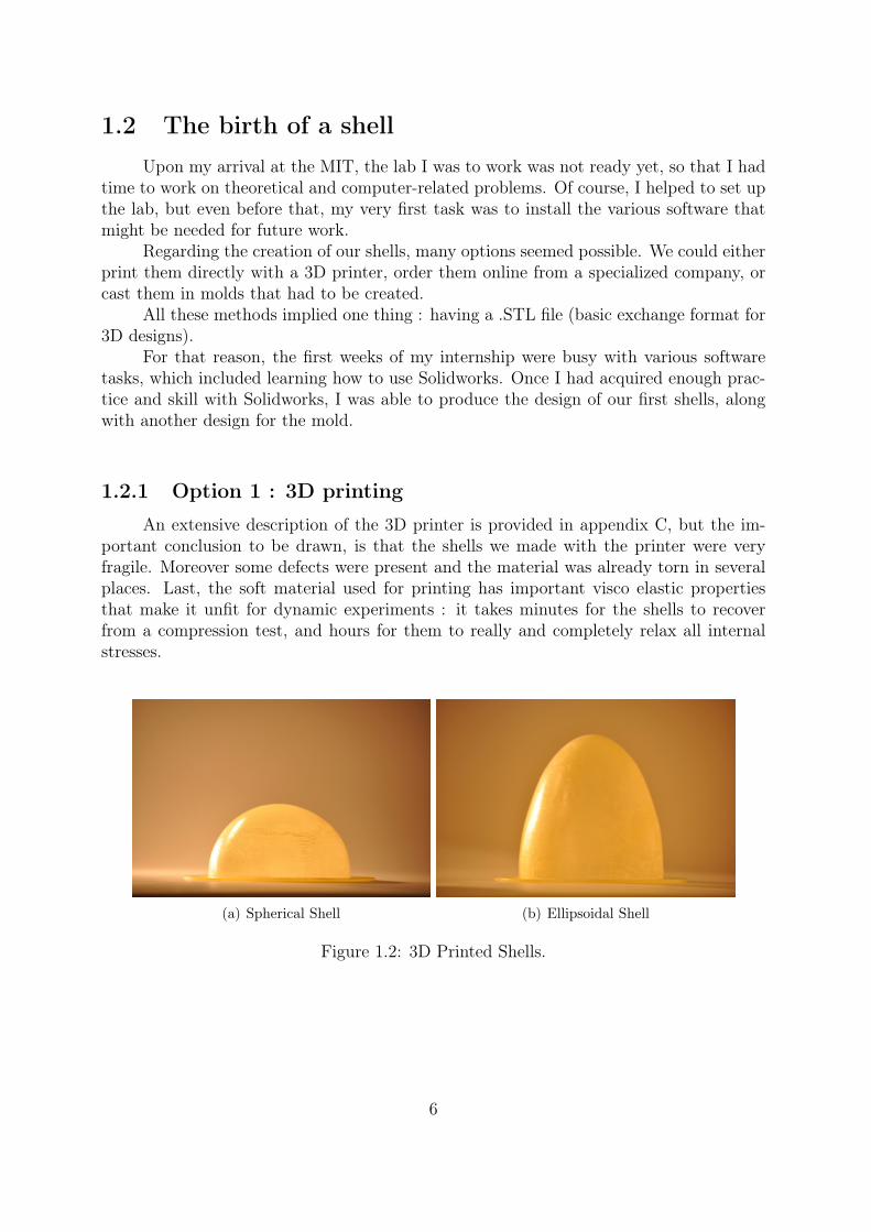
An extensive description of the 3D printer is provided in appendix C, but the im-portant conclusion to be drawn, is that the shells we made with the printer were veryfragile. Moreover some defects were present and the material was already torn in severalplaces. Last, the soft material used for printing has important visco elastic propertiesthat make it unfit for dynamic experiments : it takes minutes for the shells to recoverfrom a compression test, and hours for them to really and completely relax all internalstresses.
(a) Spherical Shell (b) Ellipsoidal Shell
Figure 1.2: 3D Printed Shells.
6
(c) Spherical Shell under point load (d) Ellipsoidal Shell under point load
Figure 1.2: 3D Printed Shells.
Still, it was useful to have these shells, we used them when studying the linearregime, cf part 1.4.1. Moreover their big size and transparency made them appropriatefor imaging purposes.
1.2.2 Option 2 : Casting
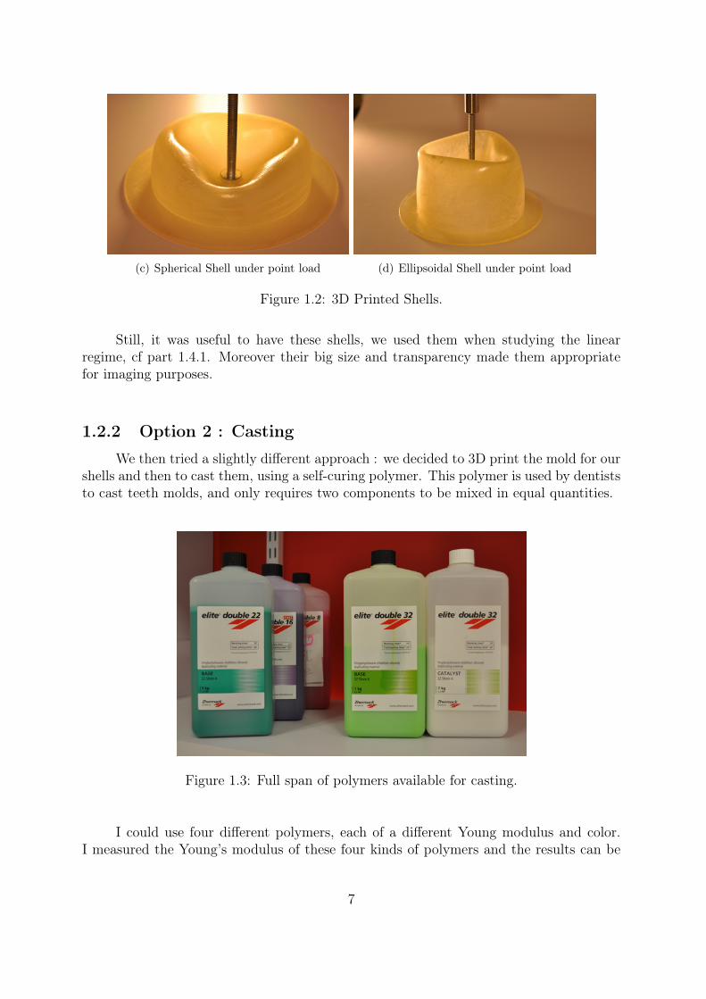
We then tried a slightly different approach : we decided to 3D print the mold for ourshells and then to cast them, using a self-curing polymer. This polymer is used by dentiststo cast teeth molds, and only requires two components to be mixed in equal quantities.
Figure 1.3: Full span of polymers available for casting.
I could use four different polymers, each of a different Young modulus and color.I measured the Young’s modulus of these four kinds of polymers and the results can be
7
found in appendix A.
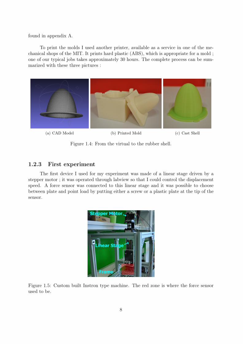
To print the molds I used another printer, available as a service in one of the me-chanical shops of the MIT. It prints hard plastic (ABS), which is appropriate for a mold ;one of our typical jobs takes approximately 30 hours. The complete process can be sum-marized with these three pictures :
(a) CAD Model (b) Printed Mold (c) Cast Shell
Figure 1.4: From the virtual to the rubber shell.
1.2.3 First experiment
The first device I used for my experiment was made of a linear stage driven by astepper motor ; it was operated through labview so that I could control the displacementspeed. A force sensor was connected to this linear stage and it was possible to choosebetween plate and point load by putting either a screw or a plastic plate at the tip of thesensor.
Figure 1.5: Custom built Instron type machine. The red zone is where the force sensorused to be.
8
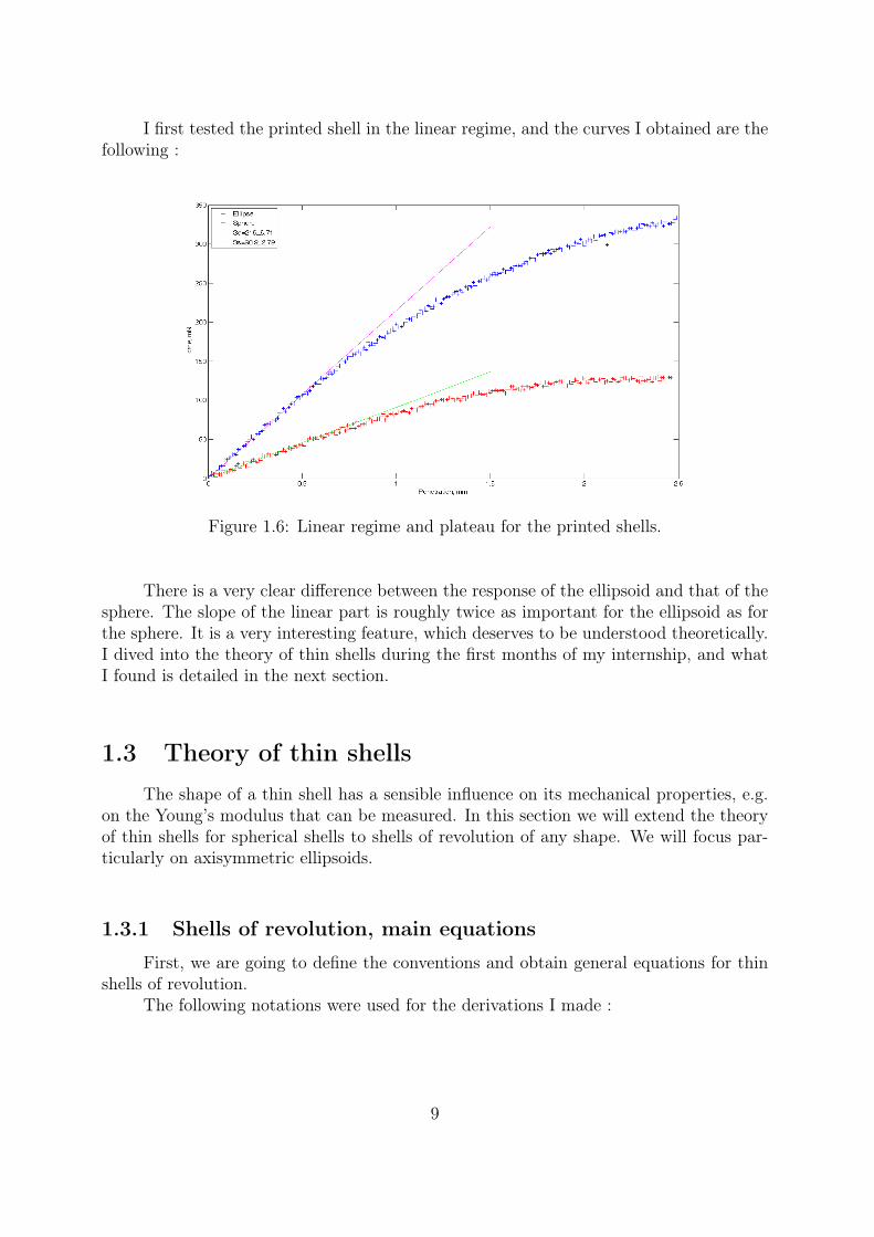
I first tested the printed shell in the linear regime, and the curves I obtained are thefollowing :
Figure 1.6: Linear regime and plateau for the printed shells.
There is a very clear difference between the response of the ellipsoid and that of thesphere. The slope of the linear part is roughly twice as important for the ellipsoid as forthe sphere. It is a very interesting feature, which deserves to be understood theoretically.I dived into the theory of thin shells during the first months of my internship, and whatI found is detailed in the next section.
1.3 Theory of thin shellsThe shape of a thin shell has a sensible influence on its mechanical properties, e.g.
on the Young’s modulus that can be measured. In this section we will extend the theoryof thin shells for spherical shells to shells of revolution of any shape. We will focus par-ticularly on axisymmetric ellipsoids.
1.3.1 Shells of revolution, main equations
First, we are going to define the conventions and obtain general equations for thinshells of revolution.
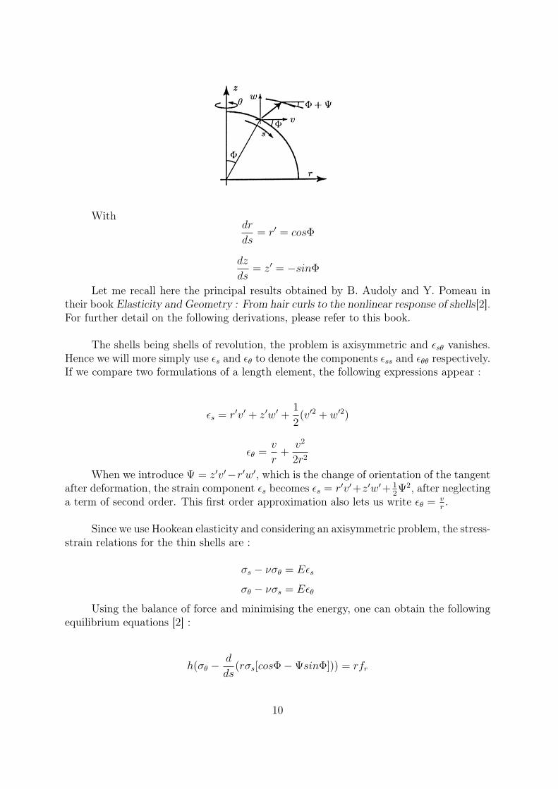
The following notations were used for the derivations I made :
9
Withdr
ds= r′ = cosΦ
dz
ds= z′ = −sinΦ
Let me recall here the principal results obtained by B. Audoly and Y. Pomeau intheir book Elasticity and Geometry : From hair curls to the nonlinear response of shells[2].For further detail on the following derivations, please refer to this book.
The shells being shells of revolution, the problem is axisymmetric and εsθ vanishes.Hence we will more simply use εs and εθ to denote the components εss and εθθ respectively.If we compare two formulations of a length element, the following expressions appear :
εs = r′v′ + z′w′ +1
2(v′2 + w′2)
εθ =v
r+
v2
2r2
When we introduce Ψ = z′v′−r′w′, which is the change of orientation of the tangentafter deformation, the strain component εs becomes εs = r′v′+z′w′+ 1
2Ψ2, after neglecting
a term of second order. This first order approximation also lets us write εθ = vr.
Since we use Hookean elasticity and considering an axisymmetric problem, the stress-strain relations for the thin shells are :
σs − νσθ = Eεs
σθ − νσs = Eεθ
Using the balance of force and minimising the energy, one can obtain the followingequilibrium equations [2] :
h(σθ −d
ds(rσs[cosΦ−ΨsinΦ])) = rfr
10
h(d
ds(rσs[sinΦ + ΨcosΦ] +
D
h[(r∆w)′ −∆w])) = rfz
Where D = Eh3
12(1−ν2)and w is the displacement along the vertical axis.
1.3.2 Ellipsoids of revolution
The equations obtained previously are valid for shells of revolution of any shape.From now on, we shall concentrate on shells of ellipsoidal shape.
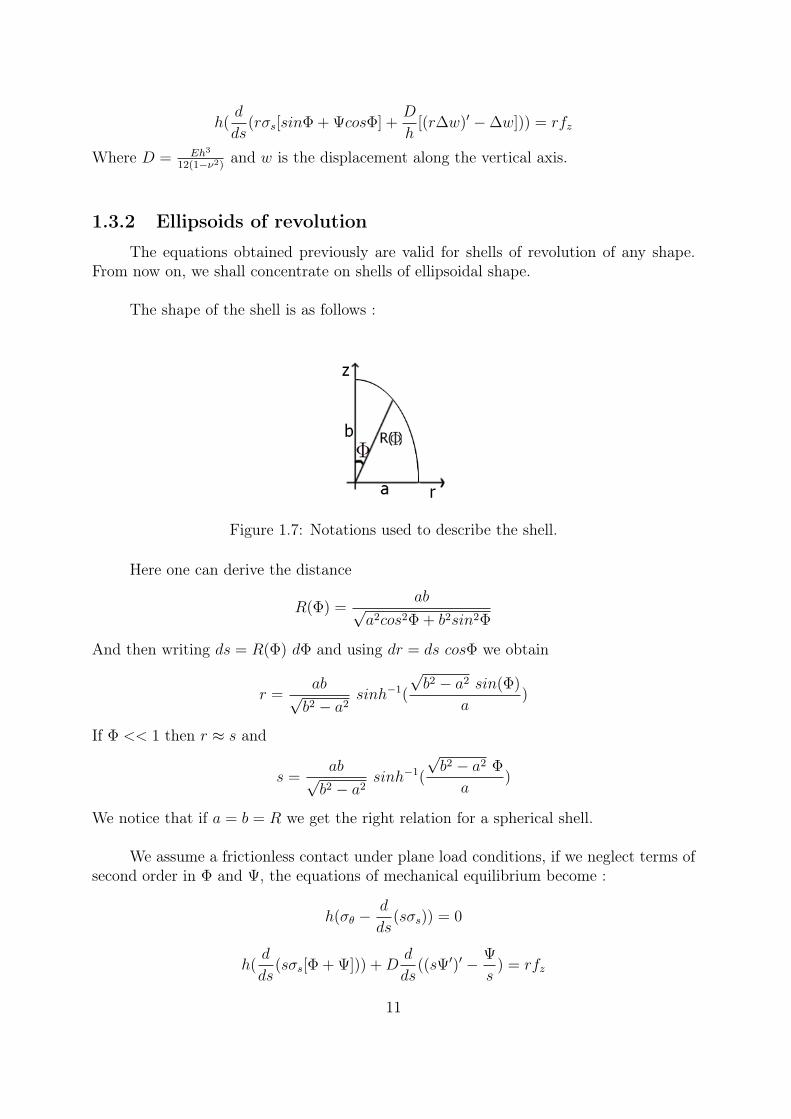
The shape of the shell is as follows :
Figure 1.7: Notations used to describe the shell.
Here one can derive the distance
R(Φ) =ab√
a2cos2Φ + b2sin2Φ
And then writing ds = R(Φ) dΦ and using dr = ds cosΦ we obtain
r =ab√b2 − a2
sinh−1(
√b2 − a2 sin(Φ)
a)
If Φ << 1 then r ≈ s and
s =ab√b2 − a2
sinh−1(
√b2 − a2 Φ
a)
We notice that if a = b = R we get the right relation for a spherical shell.
We assume a frictionless contact under plane load conditions, if we neglect terms ofsecond order in Φ and Ψ, the equations of mechanical equilibrium become :
h(σθ −d
ds(sσs)) = 0
h(d
ds(sσs[Φ + Ψ])) +D
d
ds((sΨ′)′ − Ψ
s) = rfz
11
Thus we find that σθ = (sσs)′, and using the equations above to eliminate σθ one
can obtain the dimensionless equation :
s2σ′′s + 3sσ′s + ΦΨ + 1/2Ψ2 = 0
If we consider a disc-like contact under a plane load, the following relation is alwaystrue on the contact zone Ψ + Φ = 0, i.e. the contact zone is flat. Hence the equationabove becomes :
s2σ′′s + 3sσ′s − 1/2Φ2 = 0
We then define δ =√b2 − a2 and R =
√ab to write Φ = a
δsinh( sδ
R).
This leads to the final differential equation we have to solve to know the stress inthe disc-like contact region with a plane load :
s2σ′′s + 3sσ′s =a2
2δ2sinh2(
sδ
R)
In the approximation of small deformations where s/R << 1, this equation becomes
s2σ′′s + 3sσ′s =a
b
s2
2
By integration of this equation we obtain
σs,ellipsoid =a
bσs,sphere ∝
a
b
s2
16
Thus the only difference with a spherical shell of revolution is a factor a/b for the radialstress σs,sphere ∝ s2
16.
Using the stress-strain relation
σs,ellipsoid − ν(sσs,ellipsoid)′ =
a
b[σs,sphere − ν(sσs,sphere)
′] = Eεs
we clearly see that the ellipsoid problem is the same as the spherical one, provided weconsider an effective Young’s modulus Eeff = b
aE for the ellipsoid.
This very simple theoretical result means that a shell twice as high as a sphericalshell should be twice as stiff. We will verify it experimentally, by testing the mechanicalresponse of various shell geometries in the linear regime.
1.4 ExperimentsGeometrically induced rigidity of shells can be probed easily by doing compression
tests. Two domains can be studied, the linear regime, and the nonlinear one, in whicha localization of the stress is to be seen. In the experiments described throughout thissection I made extensive use of a laser cutter, (for more details on this exceptional tool,
12
please see appendix D).
Systematic experiments could begin when my home made force sensor was replacedby a commercial Instron. With the Instron’s load cell new limit of 10 N, I could explorethe whole behavior of the shells, without having to see the sensor saturate after the firstfew millimeters. We actually found the Instron impossible to use because its generic load-ing system was too heavy for our very sensitive load cell. Therefore we had to deviseanother loading system.
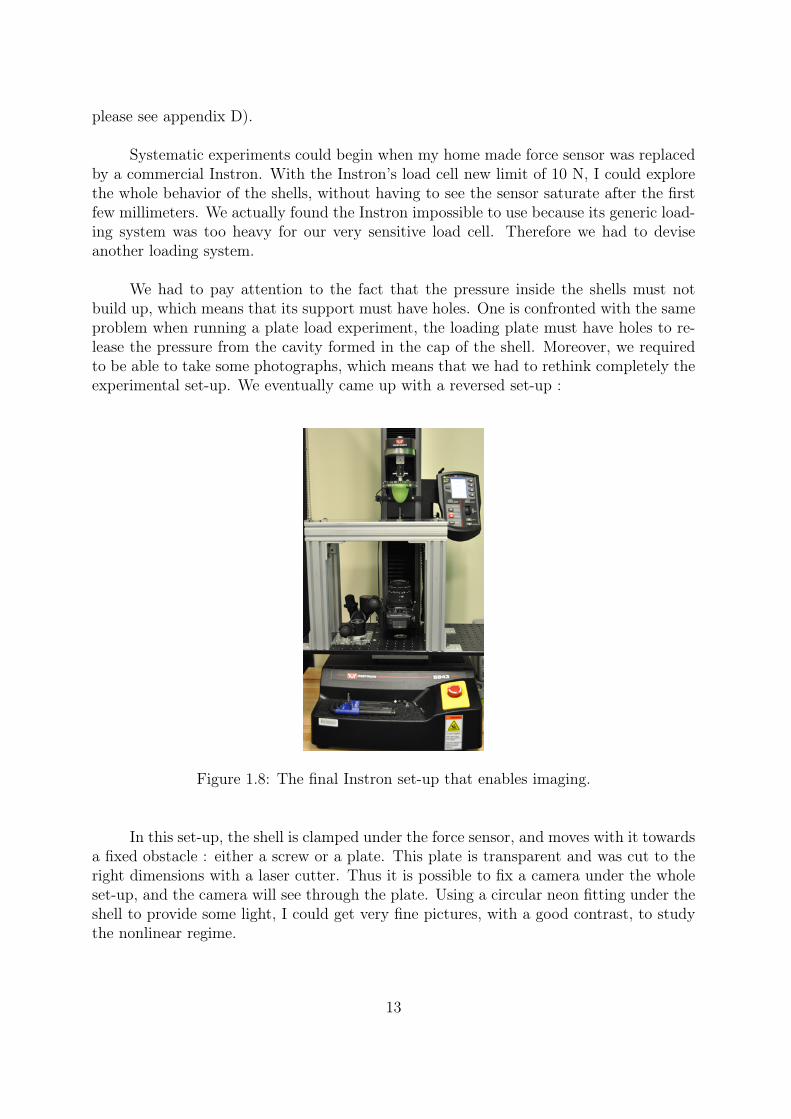
We had to pay attention to the fact that the pressure inside the shells must notbuild up, which means that its support must have holes. One is confronted with the sameproblem when running a plate load experiment, the loading plate must have holes to re-lease the pressure from the cavity formed in the cap of the shell. Moreover, we requiredto be able to take some photographs, which means that we had to rethink completely theexperimental set-up. We eventually came up with a reversed set-up :
Figure 1.8: The final Instron set-up that enables imaging.
In this set-up, the shell is clamped under the force sensor, and moves with it towardsa fixed obstacle : either a screw or a plate. This plate is transparent and was cut to theright dimensions with a laser cutter. Thus it is possible to fix a camera under the wholeset-up, and the camera will see through the plate. Using a circular neon fitting under theshell to provide some light, I could get very fine pictures, with a good contrast, to studythe nonlinear regime.
13
1.4.1 Linear Regime
By experimenting on the linear regime we can measure the stiffness of a structure,i.e. its effective Young’s modulus. We have just seen that the effective Young’s modulusmeasured should grow linearly with the ratio b/a, where b and a are respectively the largeand the small radii of the ellipsoid of revolution. (cf section 1.3)
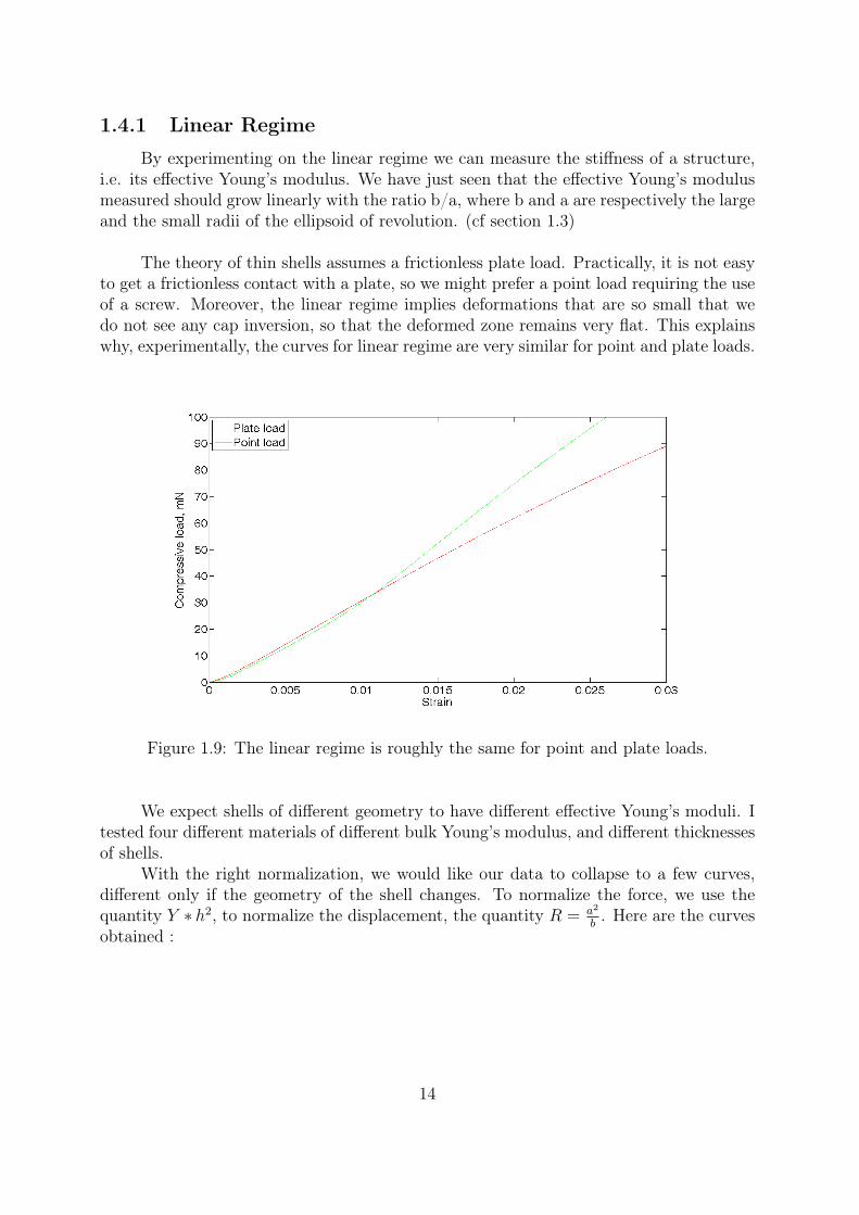
The theory of thin shells assumes a frictionless plate load. Practically, it is not easyto get a frictionless contact with a plate, so we might prefer a point load requiring the useof a screw. Moreover, the linear regime implies deformations that are so small that wedo not see any cap inversion, so that the deformed zone remains very flat. This explainswhy, experimentally, the curves for linear regime are very similar for point and plate loads.
Figure 1.9: The linear regime is roughly the same for point and plate loads.
We expect shells of different geometry to have different effective Young’s moduli. Itested four different materials of different bulk Young’s modulus, and different thicknessesof shells.
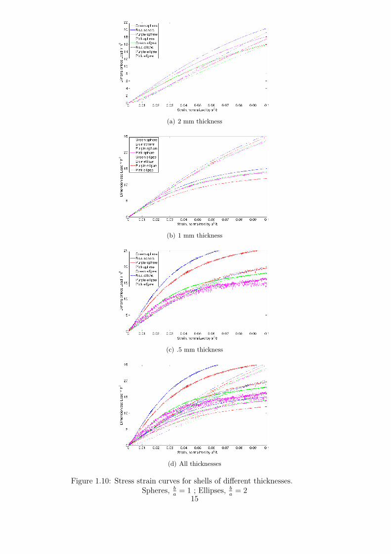
With the right normalization, we would like our data to collapse to a few curves,different only if the geometry of the shell changes. To normalize the force, we use thequantity Y ∗ h2, to normalize the displacement, the quantity R = a2
b. Here are the curves
obtained :
14
(a) 2 mm thickness
(b) 1 mm thickness
(c) .5 mm thickness
(d) All thicknesses
Figure 1.10: Stress strain curves for shells of different thicknesses.Spheres, b
a= 1 ; Ellipses, b
a= 2
15
This normalization works well, because it takes into account the difference in geom-etry when normalizing the strain, and the difference in thickness when normalizing theforce.
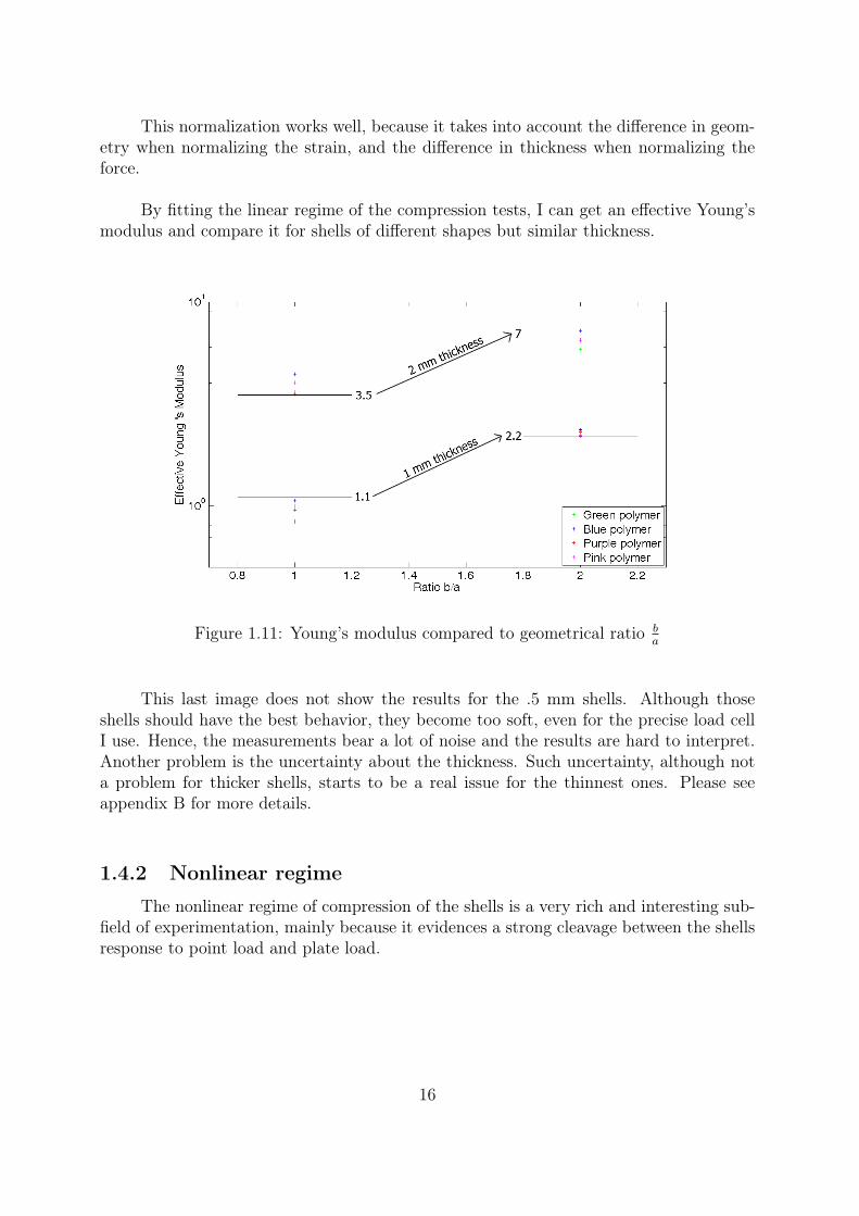
By fitting the linear regime of the compression tests, I can get an effective Young’smodulus and compare it for shells of different shapes but similar thickness.
Figure 1.11: Young’s modulus compared to geometrical ratio ba
This last image does not show the results for the .5 mm shells. Although thoseshells should have the best behavior, they become too soft, even for the precise load cellI use. Hence, the measurements bear a lot of noise and the results are hard to interpret.Another problem is the uncertainty about the thickness. Such uncertainty, although nota problem for thicker shells, starts to be a real issue for the thinnest ones. Please seeappendix B for more details.
1.4.2 Nonlinear regime
The nonlinear regime of compression of the shells is a very rich and interesting sub-field of experimentation, mainly because it evidences a strong cleavage between the shellsresponse to point load and plate load.
16
Point load, localization of the stress
Under point load, the behavior observed is first a progressive inversion of the capof the shell, but after ≈ 80% strain, the stress localizes into ridges forming geometricalfigures (e.g. triangles).
This behavior has nothing to do with the material used : it depends only on geo-metrical properties. For example, a shell twice as big and thick as another one, will havethe same localization patterns.
This experiment was done on the 1 mm thick ellipsoid shells ( ba
= 2, a = 25 mm),and I compared the four different materials I dipsosed of. Using a very low strain-rate,photographs were taken every 10 seconds, which allows us to track the position of theridges. Superposition of the result leads to this graph :
(a) Position of the ridges (b) Typical stress strain curve obtained.
Figure 1.12: Position of the ridges under large deformation point load. 1 mm thick shells.
The farther from the center the points are, the larger the deformation is. First, wesee that all shells show the same behavior ; localization into a triangular shape, and theninto a square. The transition between the triangle and the square pattern is very hard totrack, but a new ridge seems to appear between two others, the other ridges then migratea little to form a square.
This localization pattern depends only on the size and on the thickness of the shell.The only other shells thin enough to show localization I had were the .5 mm, on whichI ran the same experiment. They have exactly the same pattern : they form a triangle,then a square.
Plate load, buckling
Under plate load, the shells do not invert their cap, but buckle instead. The buck-ling occurs on the middle of the shell and looks like this :
17
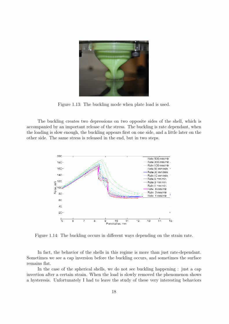
Figure 1.13: The buckling mode when plate load is used.
The buckling creates two depressions on two opposite sides of the shell, which isaccompanied by an important release of the stress. The buckling is rate dependant, whenthe loading is slow enough, the buckling appears first on one side, and a little later on theother side. The same stress is released in the end, but in two steps.
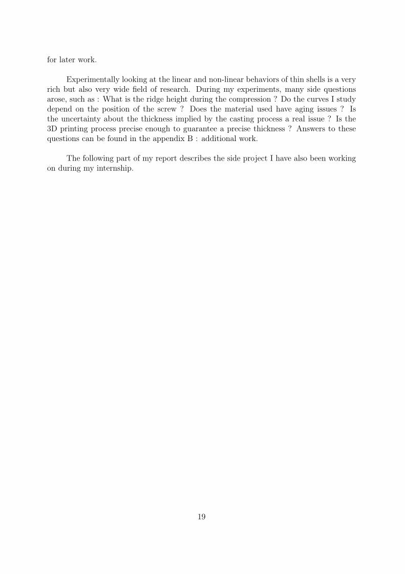
Figure 1.14: The buckling occurs in different ways depending on the strain rate.
In fact, the behavior of the shells in this regime is more than just rate-dependant.Sometimes we see a cap inversion before the buckling occurs, and sometimes the surfaceremains flat.
In the case of the spherical shells, we do not see buckling happening : just a capinvertion after a certain strain. When the load is slowly removed the phenomenon showsa hysteresis. Unfortunately I had to leave the study of these very interesting behaviors
18
for later work.
Experimentally looking at the linear and non-linear behaviors of thin shells is a veryrich but also very wide field of research. During my experiments, many side questionsarose, such as : What is the ridge height during the compression ? Do the curves I studydepend on the position of the screw ? Does the material used have aging issues ? Isthe uncertainty about the thickness implied by the casting process a real issue ? Is the3D printing process precise enough to guarantee a precise thickness ? Answers to thesequestions can be found in the appendix B : additional work.
The following part of my report describes the side project I have also been workingon during my internship.
19
Chapter 2
Negative Poisson’s ratio structures
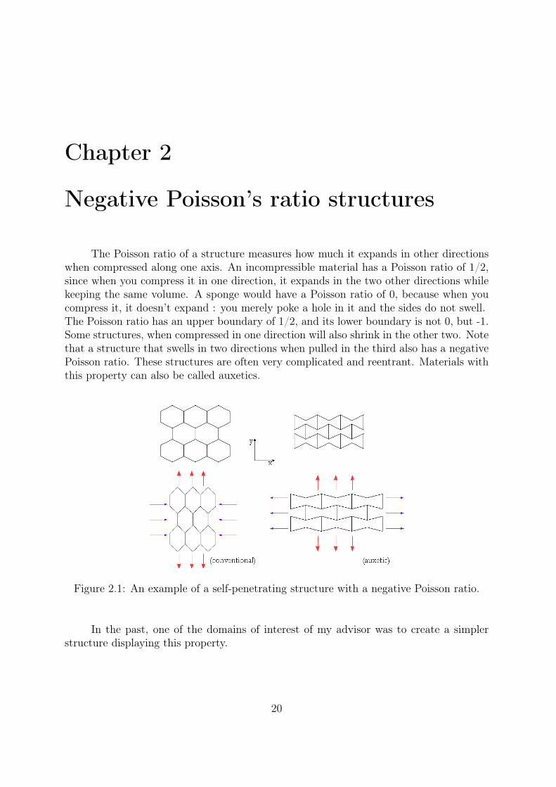
The Poisson ratio of a structure measures how much it expands in other directionswhen compressed along one axis. An incompressible material has a Poisson ratio of 1/2,since when you compress it in one direction, it expands in the two other directions whilekeeping the same volume. A sponge would have a Poisson ratio of 0, because when youcompress it, it doesn’t expand : you merely poke a hole in it and the sides do not swell.The Poisson ratio has an upper boundary of 1/2, and its lower boundary is not 0, but -1.Some structures, when compressed in one direction will also shrink in the other two. Notethat a structure that swells in two directions when pulled in the third also has a negativePoisson ratio. These structures are often very complicated and reentrant. Materials withthis property can also be called auxetics.
Figure 2.1: An example of a self-penetrating structure with a negative Poisson ratio.
In the past, one of the domains of interest of my advisor was to create a simplerstructure displaying this property.
20
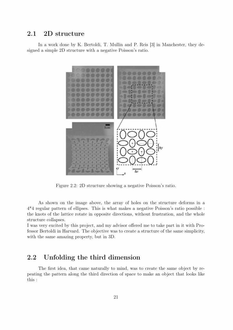
2.1 2D structureIn a work done by K. Bertoldi, T. Mullin and P. Reis [3] in Manchester, they de-
signed a simple 2D structure with a negative Poisson’s ratio.
Figure 2.2: 2D structure showing a negative Poisson’s ratio.
As shown on the image above, the array of holes on the structure deforms in a4*4 regular pattern of ellipses. This is what makes a negative Poisson’s ratio possible :the knots of the lattice rotate in opposite directions, without frustration, and the wholestructure collapses.I was very excited by this project, and my advisor offered me to take part in it with Pro-fessor Bertoldi in Harvard. The objective was to create a structure of the same simplicity,with the same amazing property, but in 3D.
2.2 Unfolding the third dimensionThe first idea, that came naturally to mind, was to create the same object by re-
peating the pattern along the third direction of space to make an object that looks likethis :
21
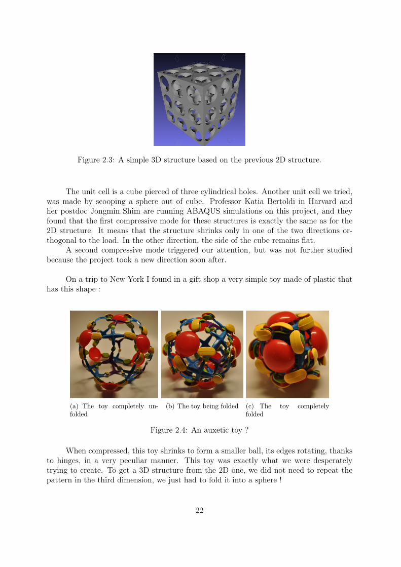
Figure 2.3: A simple 3D structure based on the previous 2D structure.
The unit cell is a cube pierced of three cylindrical holes. Another unit cell we tried,was made by scooping a sphere out of cube. Professor Katia Bertoldi in Harvard andher postdoc Jongmin Shim are running ABAQUS simulations on this project, and theyfound that the first compressive mode for these structures is exactly the same as for the2D structure. It means that the structure shrinks only in one of the two directions or-thogonal to the load. In the other direction, the side of the cube remains flat.
A second compressive mode triggered our attention, but was not further studiedbecause the project took a new direction soon after.
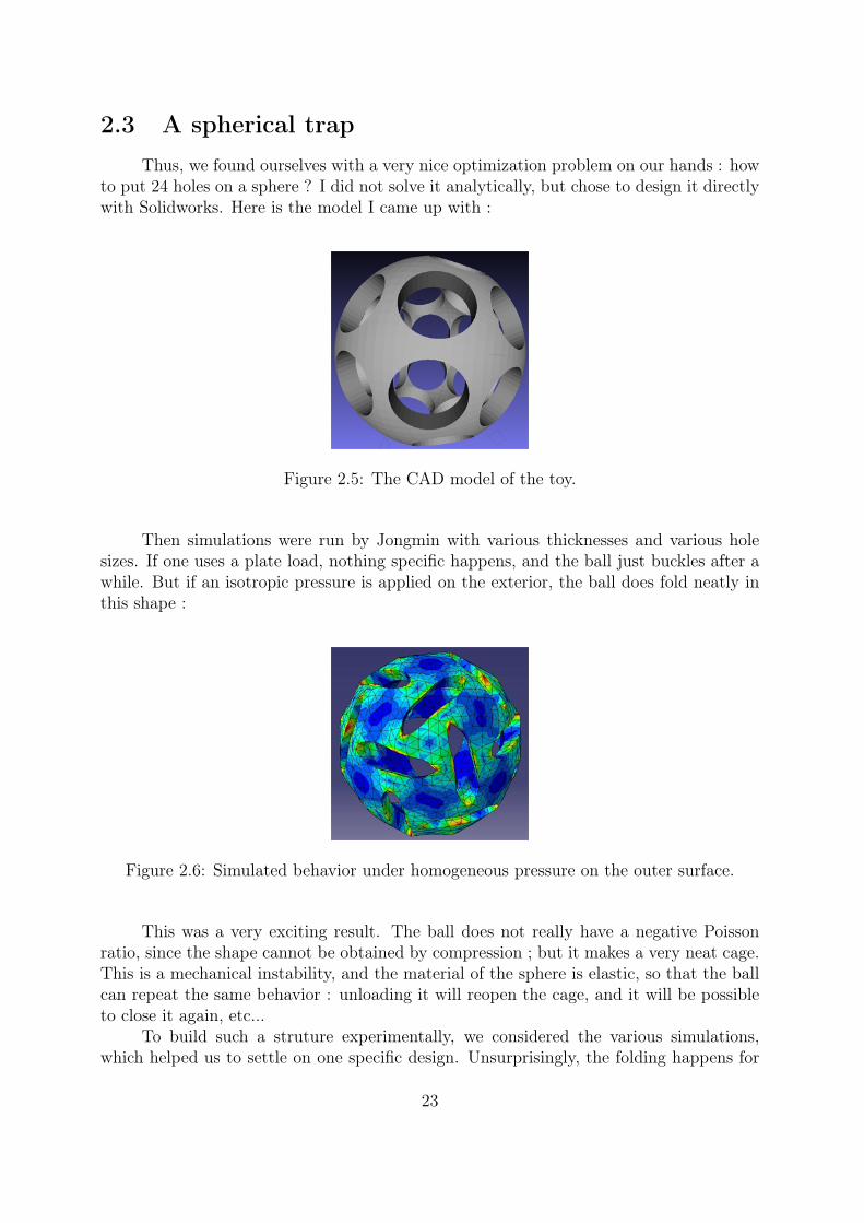
On a trip to New York I found in a gift shop a very simple toy made of plastic thathas this shape :
(a) The toy completely un-folded
(b) The toy being folded (c) The toy completelyfolded
Figure 2.4: An auxetic toy ?
When compressed, this toy shrinks to form a smaller ball, its edges rotating, thanksto hinges, in a very peculiar manner. This toy was exactly what we were desperatelytrying to create. To get a 3D structure from the 2D one, we did not need to repeat thepattern in the third dimension, we just had to fold it into a sphere !
22
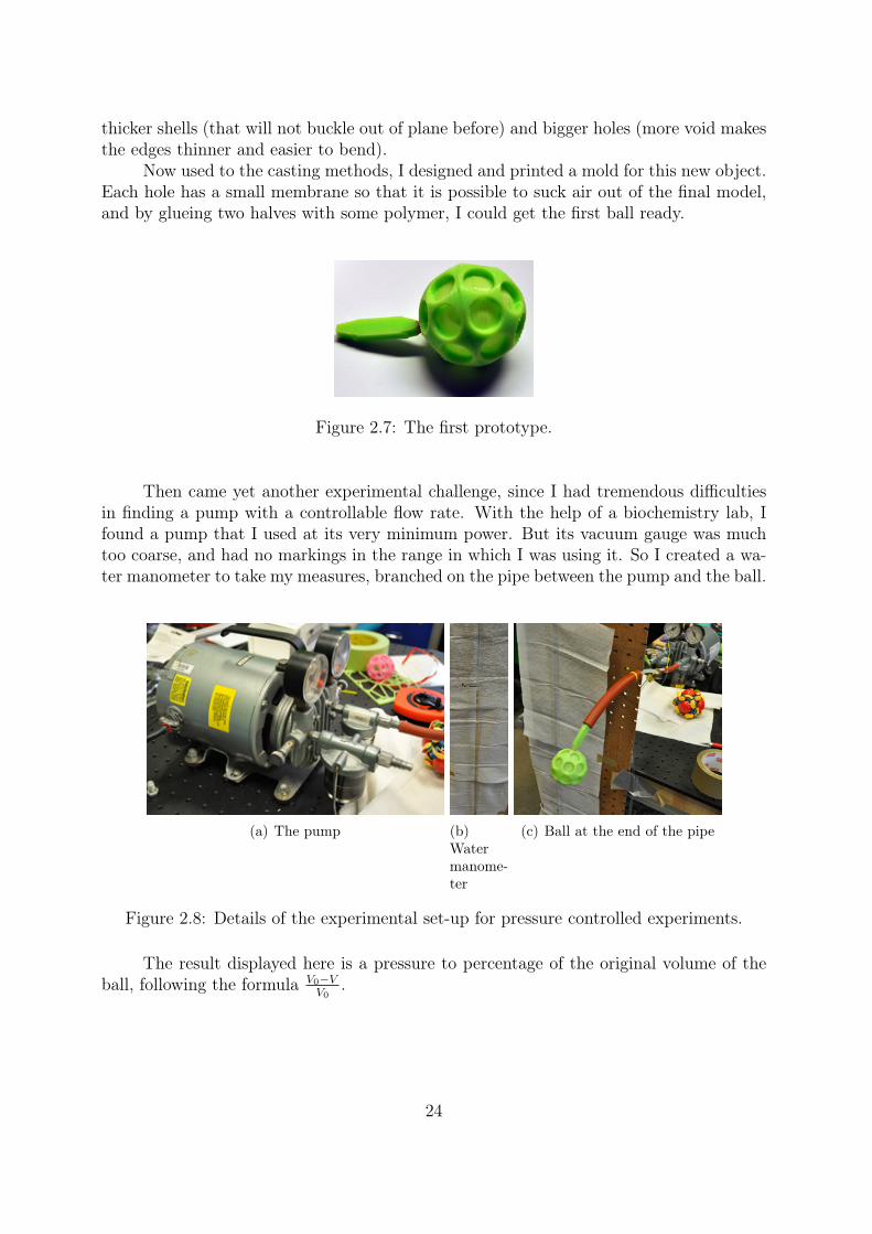
2.3 A spherical trapThus, we found ourselves with a very nice optimization problem on our hands : how
to put 24 holes on a sphere ? I did not solve it analytically, but chose to design it directlywith Solidworks. Here is the model I came up with :
Figure 2.5: The CAD model of the toy.
Then simulations were run by Jongmin with various thicknesses and various holesizes. If one uses a plate load, nothing specific happens, and the ball just buckles after awhile. But if an isotropic pressure is applied on the exterior, the ball does fold neatly inthis shape :
Figure 2.6: Simulated behavior under homogeneous pressure on the outer surface.
This was a very exciting result. The ball does not really have a negative Poissonratio, since the shape cannot be obtained by compression ; but it makes a very neat cage.This is a mechanical instability, and the material of the sphere is elastic, so that the ballcan repeat the same behavior : unloading it will reopen the cage, and it will be possibleto close it again, etc...
To build such a struture experimentally, we considered the various simulations,which helped us to settle on one specific design. Unsurprisingly, the folding happens for
23
thicker shells (that will not buckle out of plane before) and bigger holes (more void makesthe edges thinner and easier to bend).
Now used to the casting methods, I designed and printed a mold for this new object.Each hole has a small membrane so that it is possible to suck air out of the final model,and by glueing two halves with some polymer, I could get the first ball ready.
Figure 2.7: The first prototype.
Then came yet another experimental challenge, since I had tremendous difficultiesin finding a pump with a controllable flow rate. With the help of a biochemistry lab, Ifound a pump that I used at its very minimum power. But its vacuum gauge was muchtoo coarse, and had no markings in the range in which I was using it. So I created a wa-ter manometer to take my measures, branched on the pipe between the pump and the ball.
(a) The pump (b)Watermanome-ter
(c) Ball at the end of the pipe
Figure 2.8: Details of the experimental set-up for pressure controlled experiments.
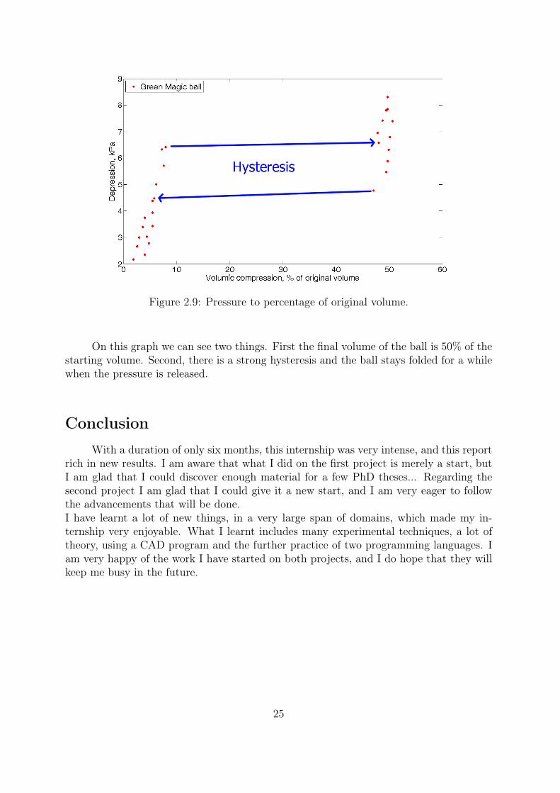
The result displayed here is a pressure to percentage of the original volume of theball, following the formula V0−V
V0.
24
Figure 2.9: Pressure to percentage of original volume.
On this graph we can see two things. First the final volume of the ball is 50% of thestarting volume. Second, there is a strong hysteresis and the ball stays folded for a whilewhen the pressure is released.
ConclusionWith a duration of only six months, this internship was very intense, and this report
rich in new results. I am aware that what I did on the first project is merely a start, butI am glad that I could discover enough material for a few PhD theses... Regarding thesecond project I am glad that I could give it a new start, and I am very eager to followthe advancements that will be done.I have learnt a lot of new things, in a very large span of domains, which made my in-ternship very enjoyable. What I learnt includes many experimental techniques, a lot oftheory, using a CAD program and the further practice of two programming languages. Iam very happy of the work I have started on both projects, and I do hope that they willkeep me busy in the future.
25
AcknowledgmentsI would like to thank warmly Pedro Reis for the opportunity he gave me to spend 6
months in his lab at the MIT. I cannot emphasize enough how happy I was, and still amabout the whole internship both from a scientific and from a human perspective. I amalso very thankful to Katia Bertoldi, who seemed very happy to have me involved in herresearch ; I am even happier that I could contribute a little to it.
I would like to also acknowledge Jongmin Shim’s hard work and availability. I alsothank all the students from civil engineering who have helped me during the internship,especially the "Red Cement" group.
I am grateful to Professor L. Anand, who let me follow his course on Mechanics ofsolid materials.
Some very special acknowledgments go to Joël Marthelot, Fanny Mas and Jean-Arthur Olive who managed to deal with my various moods and requests during those sixmonths. They also made this internship an unforgettable experience for me. I would liketo tell the various people who came to see me in the US that they all helped me in theirpersonnal way, more than they may imagine.
My regard goes to all those involved in what follows : Mountain Dew, roller skating,underground corridors, going back to France on a two days notice, being my roommate,booking the same plane as me, doing an internship in the same town as me, helping mefind poutine in Montréal, not stealing my bikes, expired bakery, and, most of all, enteringrandom shops in New York.
26
Bibliography
[1] A. Vaziri and L. Mahadevan, Localized and extended deformations of elastic shells,Proceedings of the National Academy of Sciences of the United States of America,2008, 105, 23, p. 7913–7918.
[2] B. Audoly and Y. Pomeau, Elasticity and geometry: from hair curls to the nonlinearresponse of shells Oxford University Press, July 2010, Book.
[3] K. Bertoldi, P.M. Reis, S. Willshaw and T. Mullin, Negative Poisson’s ratio behaviorinduced by an elastic instability, Advanced Materials, 2009, 21, 1.
27
Appendix A
Measuring the Young’s modulus of thepolymer
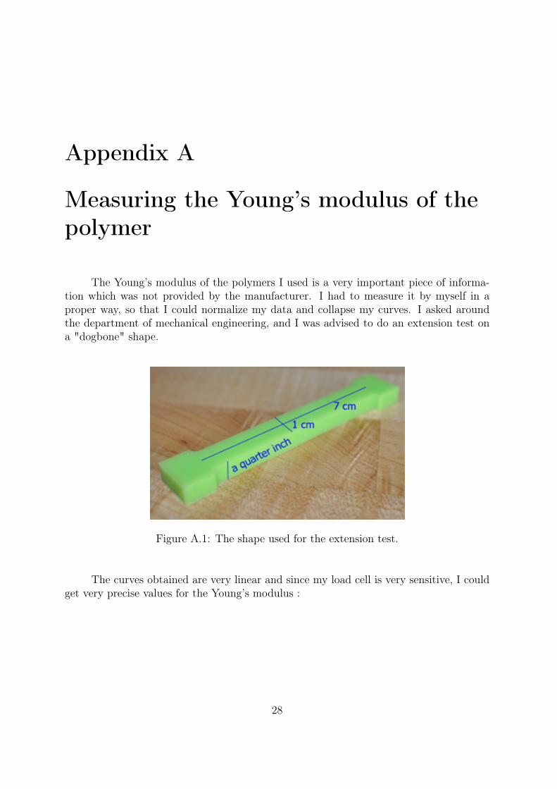
The Young’s modulus of the polymers I used is a very important piece of informa-tion which was not provided by the manufacturer. I had to measure it by myself in aproper way, so that I could normalize my data and collapse my curves. I asked aroundthe department of mechanical engineering, and I was advised to do an extension test ona "dogbone" shape.
Figure A.1: The shape used for the extension test.
The curves obtained are very linear and since my load cell is very sensitive, I couldget very precise values for the Young’s modulus :
28
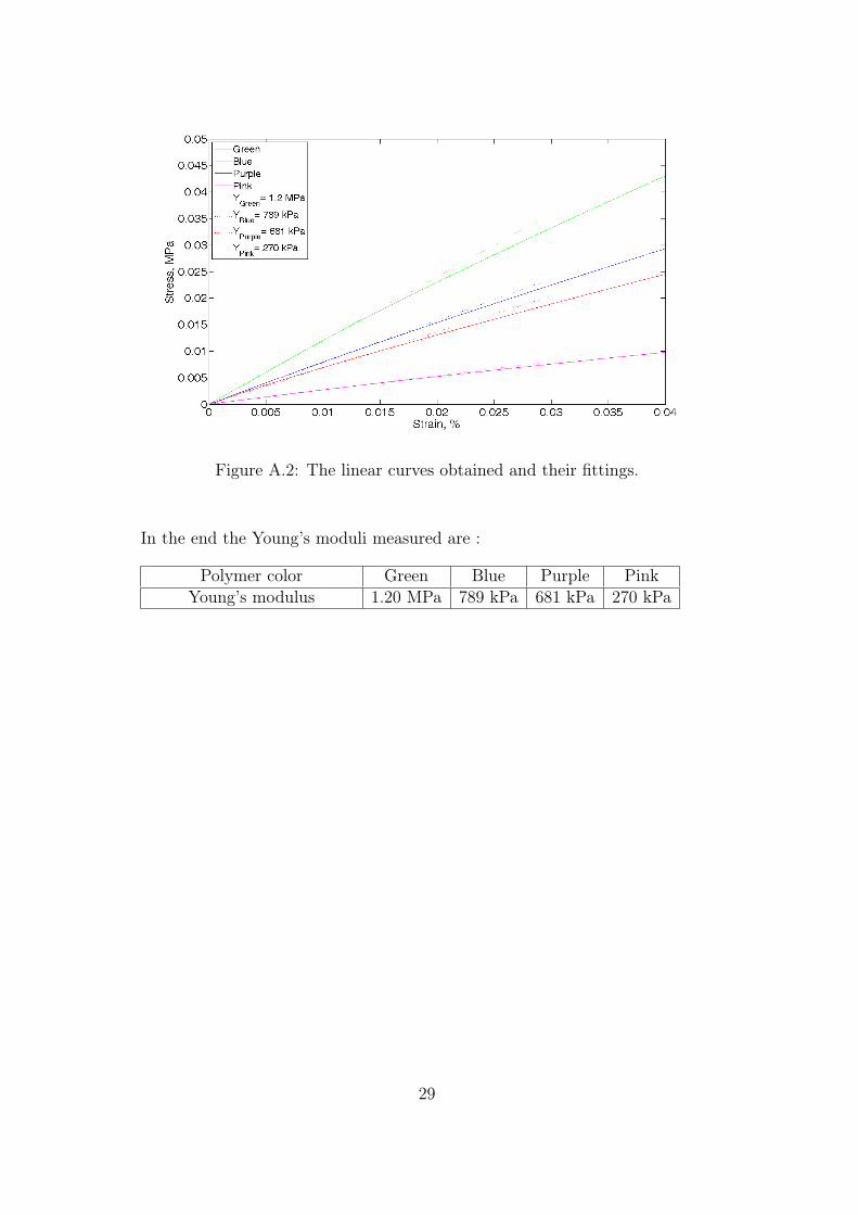
Figure A.2: The linear curves obtained and their fittings.
In the end the Young’s moduli measured are :
Polymer color Green Blue Purple PinkYoung’s modulus 1.20 MPa 789 kPa 681 kPa 270 kPa
29
Appendix B
Additional work on thin shells
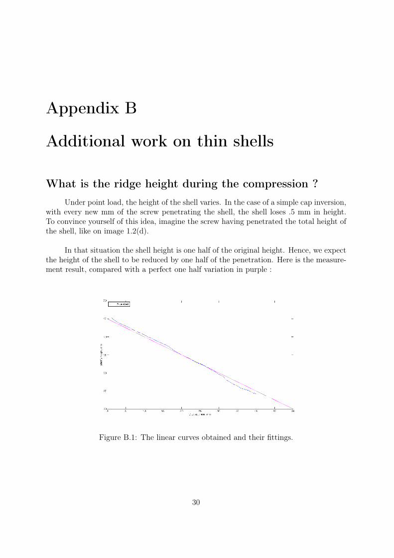
What is the ridge height during the compression ?Under point load, the height of the shell varies. In the case of a simple cap inversion,
with every new mm of the screw penetrating the shell, the shell loses .5 mm in height.To convince yourself of this idea, imagine the screw having penetrated the total height ofthe shell, like on image 1.2(d).
In that situation the shell height is one half of the original height. Hence, we expectthe height of the shell to be reduced by one half of the penetration. Here is the measure-ment result, compared with a perfect one half variation in purple :
Figure B.1: The linear curves obtained and their fittings.
30
Does the material used have aging issues ?The color of the pink shell, for example, changes over time. This means that the
polymer ages after a few weeks. But does this aging have an influence on the mechanicalproperties of the polymer ? The answer is no, as evidenced by this graph, which showstwo tests on the same shell separated by 2 months.
Figure B.2: Two tests on the same shell, separated by two months.
Is the error on the thickness implied by the casting pro-cess a real issue ?
The error on the thickness is an issue for us, because the results vary from one shellto the other. But if we cast many shells out of the same mold and then test them, we canpinpoint the error range of our measurements.
31
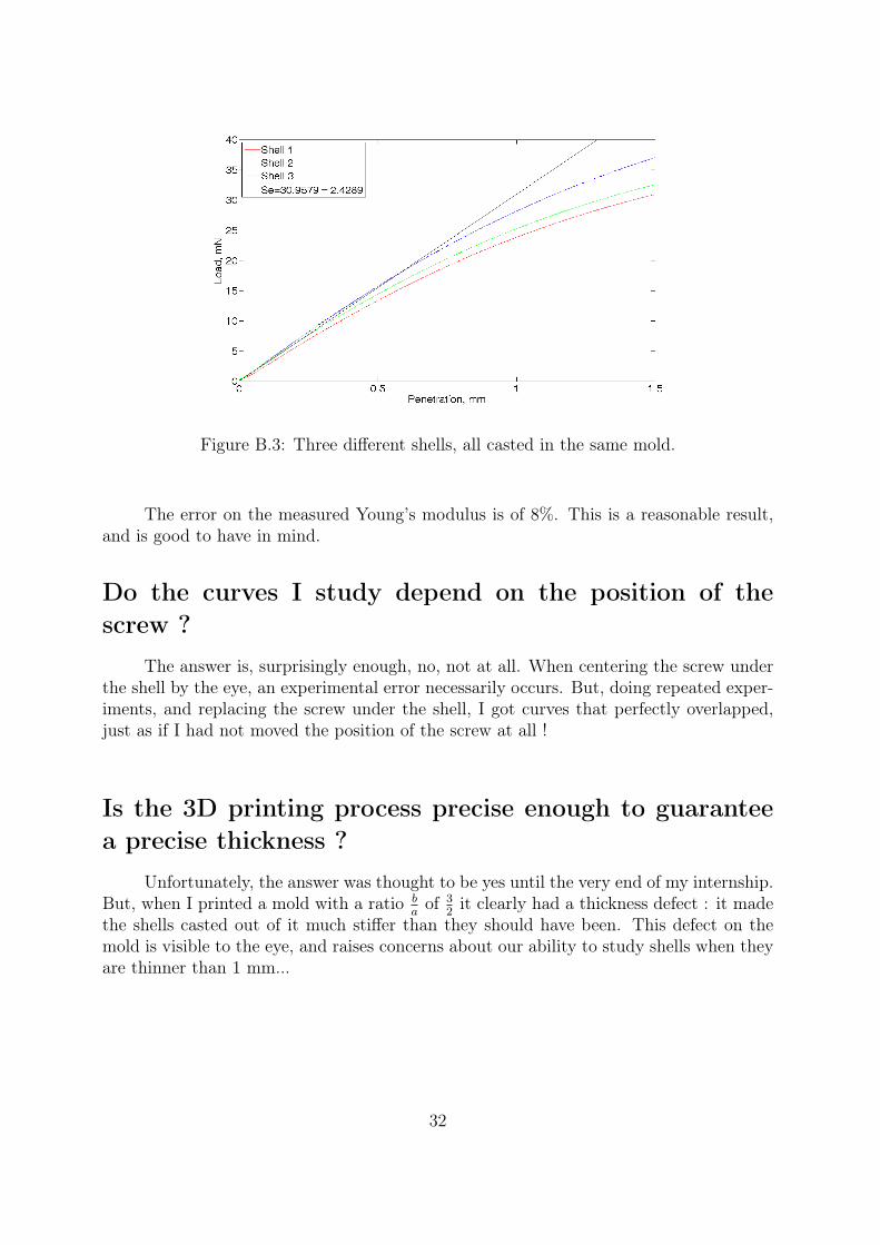
Figure B.3: Three different shells, all casted in the same mold.
The error on the measured Young’s modulus is of 8%. This is a reasonable result,and is good to have in mind.
Do the curves I study depend on the position of thescrew ?
The answer is, surprisingly enough, no, not at all. When centering the screw underthe shell by the eye, an experimental error necessarily occurs. But, doing repeated exper-iments, and replacing the screw under the shell, I got curves that perfectly overlapped,just as if I had not moved the position of the screw at all !
Is the 3D printing process precise enough to guaranteea precise thickness ?
Unfortunately, the answer was thought to be yes until the very end of my internship.But, when I printed a mold with a ratio b
aof 3
2it clearly had a thickness defect : it made
the shells casted out of it much stiffer than they should have been. This defect on themold is visible to the eye, and raises concerns about our ability to study shells when theyare thinner than 1 mm...
32
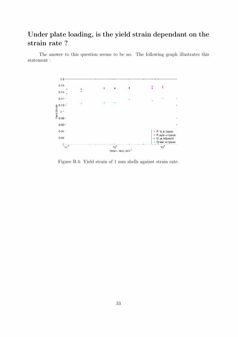
Under plate loading, is the yield strain dependant on thestrain rate ?
The answer to this question seems to be no. The following graph illustrates thisstatement :
Figure B.4: Yield strain of 1 mm shells against strain rate.
33
Appendix C
3D Printer : Connex 500
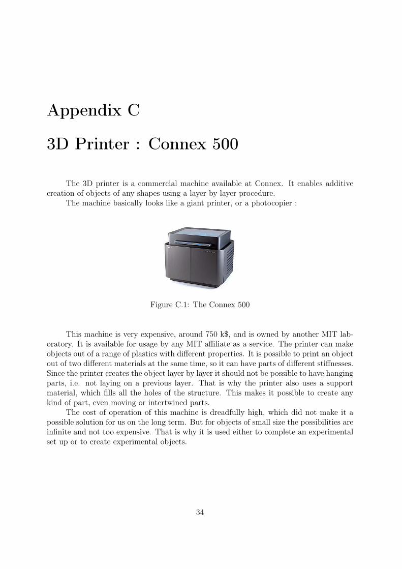
The 3D printer is a commercial machine available at Connex. It enables additivecreation of objects of any shapes using a layer by layer procedure.
The machine basically looks like a giant printer, or a photocopier :
Figure C.1: The Connex 500
This machine is very expensive, around 750 k$, and is owned by another MIT lab-oratory. It is available for usage by any MIT affiliate as a service. The printer can makeobjects out of a range of plastics with different properties. It is possible to print an objectout of two different materials at the same time, so it can have parts of different stiffnesses.Since the printer creates the object layer by layer it should not be possible to have hangingparts, i.e. not laying on a previous layer. That is why the printer also uses a supportmaterial, which fills all the holes of the structure. This makes it possible to create anykind of part, even moving or intertwined parts.
The cost of operation of this machine is dreadfully high, which did not make it apossible solution for us on the long term. But for objects of small size the possibilities areinfinite and not too expensive. That is why it is used either to complete an experimentalset up or to create experimental objects.
34
Appendix D
The Laser Cutter
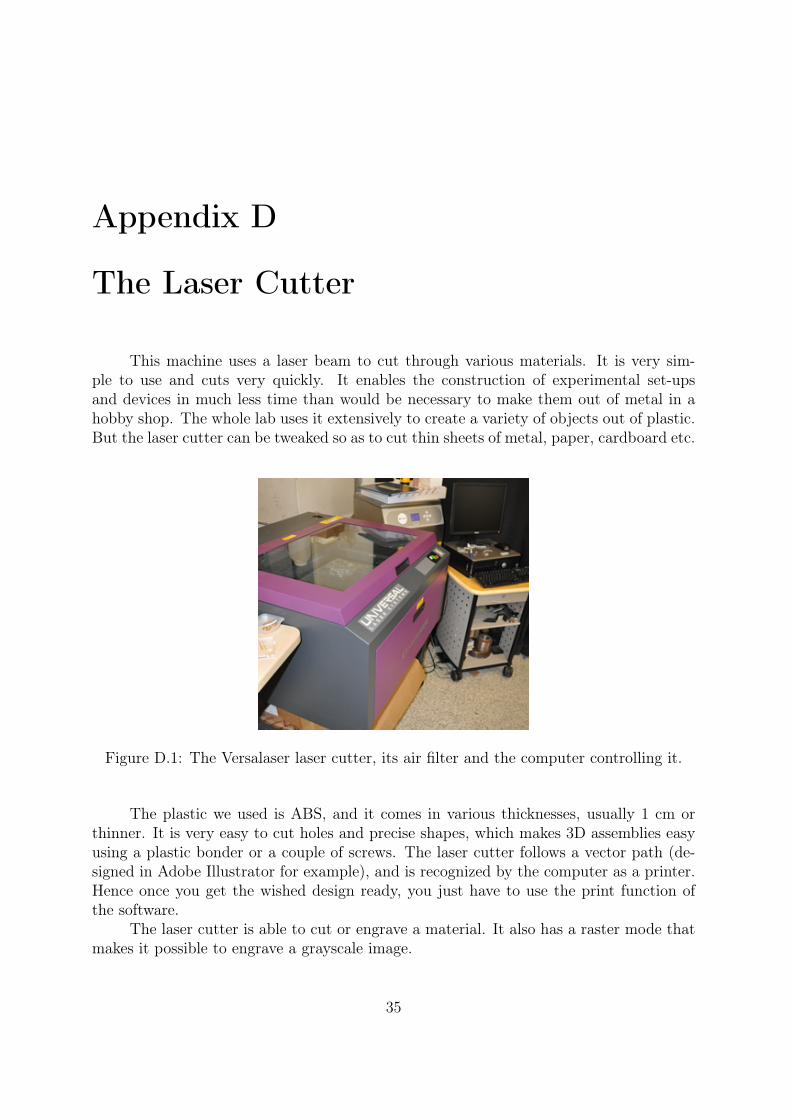
This machine uses a laser beam to cut through various materials. It is very sim-ple to use and cuts very quickly. It enables the construction of experimental set-upsand devices in much less time than would be necessary to make them out of metal in ahobby shop. The whole lab uses it extensively to create a variety of objects out of plastic.But the laser cutter can be tweaked so as to cut thin sheets of metal, paper, cardboard etc.
Figure D.1: The Versalaser laser cutter, its air filter and the computer controlling it.
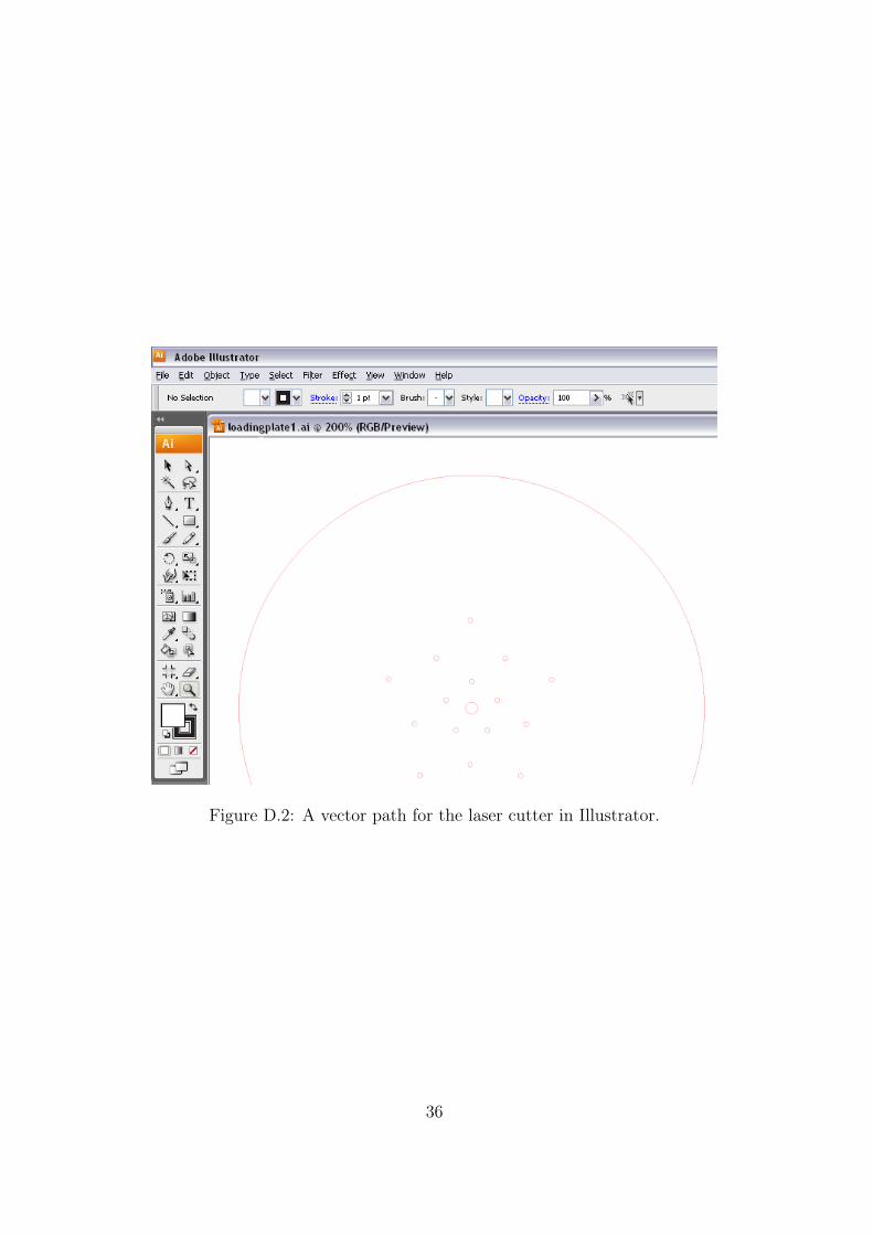
The plastic we used is ABS, and it comes in various thicknesses, usually 1 cm orthinner. It is very easy to cut holes and precise shapes, which makes 3D assemblies easyusing a plastic bonder or a couple of screws. The laser cutter follows a vector path (de-signed in Adobe Illustrator for example), and is recognized by the computer as a printer.Hence once you get the wished design ready, you just have to use the print function ofthe software.
The laser cutter is able to cut or engrave a material. It also has a raster mode thatmakes it possible to engrave a grayscale image.
35
Figure D.2: A vector path for the laser cutter in Illustrator.