Later Refraction Arrivals

in Layered Liquids

by

Robert Alden Phinney

Submitted in partial fulfillment of the requirements for

the degree of Bachelor of Science and

Master of Science in Geology and Geophysics at the

MASSACHUSETTS INSTITUTE OF TECHNOLOGY

June, 1959

Signature of AuthorRobert Alden Phinney

.0..* ..

Certified by

Head of Department

Thesis Supervisor

. .........................

R. R. Shrock.. * . 0

Abstract

Tolstoy's theory on the dispersive properties of layeredacoustic waveguides is applied to problems connected withthe detection of so-called later refraction arrivals inrefraction prospecting. His theory of antiresonant latticesis applied in a number of cases to develop a simple techniquefor estimating the dispersion curves and important later-arrival frequencies. Two cases pertinent to shallow waterproblems -have been worked out in this way, and the resultscompared with curves calculated on an IBM 704 digital com-puter. It is seen that the simple method gives predictionswhich are of fairly broad applicability, as well as providingadditional information about the modes of propagation notapparent in the exact solution.

In addition to the lattice method, other well-knownspectral considerations are brought to bear on the questionof the actual time variation of refraction arrivals. Certainfeatures are predicted whose nature must be understood inorder for a refraction record to be properly interpreted.The effects of time scaling, thickness of layers, and velocitycontrast on refraction arrivals are considered. Also dis-cussed are problems encountered in field practice whenvariables such as hydrophone depth, filtering, and recordingspeed must be optimized to obtain later refraction arrivals.Suggestions have been made for investigation of perturbationsin the layer thicknesses and predictions made of their effecton refraction arrivals.

Thable of Contents

Introduction 5

Chapter IReview of the pertinent theory 8

Chapter IIApplication to the determination ofrefracted arrivals 24

Chapter IIIDiscussion and results 32

Chapter IVConsiderations affecting the detectionand interpretation of refracted signals 42

Appendix ITable of symbols 61

Appendix IIOutline of the Buzzards Bay refractionstudy 62

Appendix IIITabulated results from the 704:Phase and group velocity for Model Ia 66Graphs of group velocity 70

Appendix IV704 program in SAP language 74

Bibliography 82

Illustrations

Figures 1 - 10 20

Figures 11 - 18 29

Plates 1 - 4 38

Plates 5 - 8 70

Acknowledgements

The author wishes to acknowledge the generous help

of Mr. Norman Ness in programming for the IBM 704 computer.

He is deeply indebted to his wife, Beth, for doing most of

the clerical work connected with preparing' this thesis.

This work was done in part at the M. I. T. Computation

Center, Cambridge, Massachusetts.

5

Introduction

In the application of seismic refraction methods to

shallow water situations, the geometry present often makes

it impossible to observe first arrivals from layers overlying

the basement. When first arrivals are observed, it is common

for the slope and intercept of the appropriate line in the

travel-time plane to be intolerably sensitive to uncertain-

ties in the data. Consequently an effort is always made to

pick intermediate layer refraction arrivals which occur

after the first arrivals from the basement. Because of

difficulties attendant on distinguishing these signals on

the disturbed trace from random fluctuations in background

level, predictions based on later arrivals are treated with

some skepticism.

As we shall see in this paper, later arrivals may dis-

play features which, if not properly understood, may lead

to wrong conclusions. At the same time, however, the

occurrence of these features may make possible positive

identification of later arrivals.

The shallow water environments to which this discussion

is applicable will generate different problems in later

arrivals picking. Typical inshore areas, such as Buzzards

Bay, Massachusetts, are best described as plane acoustic

waveguides. Consequently each refraction arrival contri-

butes an essentially undamped wave train, and the "noise"

background for later arrival picking is a superposition of

several such wave trains. In such a case we may use our

first order knowledge of the geology to help distinguish

arrivals from this noise, using the criteria to be discussed

in this paper. Typical continental shelf refraction records

tend to be less obscured by "noise" from the normal modes

than they are by hydrophone and instrument noise, due to

the higher sensitivity and amplification needed to detect

the information.

A description of later arrivals is here based on the

liquid layer theory of Pekeris, and the calculations are

performed according to the scheme of Tolstoy. It is assumed

that the reader is familiar with the theory of normal mode

propagation as discussed in GSA Memoir 27 (1958)15 and Ewing,

Jardetzky, and Press (1957)7*. The main features of

Tolstoy's work will be outlined and discussed without proof

in thispaper, since later refraction arrivals can be best

described by this rather different approach. It is also

assumed that the reader has some acquaintance with the

details of the seismic refraction technique at sea. Instru-

mentation, records, and calculations are covered in the

series of papers "Geophysical Investigations in the Emerged

and Submerged Atlantic Coastal Plaint6,9 ,10 and in GSA

Memoir 27.

Chapters I and II deal with Tolstoy's work concerning

dispersion in layered acoustic waveguides. It is shown how

* Superscripts refer to numbered references in the biblio-graphy.

the lattice approximations can be applied to two different

models to deduce the character of the dispersion without

prolonged calculation. For these cases predictions about

the later refraction arrivals are tabulated for comparison

with results obtained by a digital computer. In Chapter III

dispersion and group velocity curves for twelve different

cases as calculated on the IBM4 704 digital computer are

presented. Later arrivals deduced from these curves are

compared with prediction made by application of the lattice

approximations. The curves used to generate the lattices

are discussed in terms of the geometrical factors which

affect refraction arrivals from finite thickness layers.

The structure of the 704 program is detailed in an appendix.

The actual appearance of later arrivals is mentioned

qualitatively in Chapter IV. Criteria are developed for

intelligent picking of records. The dispersion and group

velocity curves illustrate several points. Also considered

is the question of attenuation of the refracted wave packets.

Various deviations of the geometry from that of a plan wave-

guide introduce losses by radiation into the basement and by

smearing of the energy into poorly defined wave packets by

transitions between modes. Ordinary volume scattering and

attenuation also selectively reduce the energy of refraction

arrivals. Since higher modes are generally more susceptible

to these mechanisms, the importance of low mode group velocity

maxima in determining refracted signals is emphasized.

Chapter I

Review of the Theory

The theory of sound propagation in stratified liquid

waveguides has been enunciated by Pekerisl5 , Jardetzkyll,

Tolstoy20-24, Ewing & Press8 , and others; it is not the

purpose of this paper to present or review all of this

theory, except as it touches on the problem at hand.

Pekeris15 has shown that the contribution to a steady

state acoustic potential is composed of two parts. A

branch-line integral represents the continuous spectrum,

giving rise to the transient pulse observed in seismic

refraction as the "refracted arrival.' Jardetzkyll proved

that only one branch line integral exists for an n-layered

problem, and that it was identified with the branch point

d (1)

The remainder of the signal is generated by a nonorthogonal

discrete set of modes, which arise mathematically from pole

contributions to a contour integral in the complex k-plane.

These "normal modes" constitute the principal signal observed

at long ranges, since they are caused physically by con-

structive interference of totally reflected plane waves in

the finite part of the waveguide. The normal modes are

dispersive. The horizontal phase velocity, c, is frequency

dependent; hence it is appropriate to form the group velocity:dw t e v c op

which def Ines the velocity of a wave packet with central

9

frequency "- in the waveguide. Biot2 has shown that the

group velocity is also defined for a single frequency

source (under liberal restrictions) as the rate of energy

transport in the waveguide.

The characteristic equation which defines the dispersion

of the normal modes can be obtained in straightforward

manner by application of the boundary conditions to eigen-

functions of the proper form and setting the secular deter-

minant equal to zero. For each value of c within a certain

range, there will, in general, be infinitely many solutions,

&-, , corresponding to the modes m- a 1,2,3, ..... Inversely,

for each value of w , there will be only a finite number of

Cm which solve the period equation. This is illustrated in

figures 1 and 2, where typical dispersion curves are dis-

played in the w- plane and the k-" plane.

When the sound source is a transient, it is necessary

to perform an appropriate Fourier synthesis of the steady

state solutions. If the source dependence is(-A- ( t >o)/60 = a(&e40)

its Fourier transform will be

(4)

A representation of the steady state contribution from the

normal modes is*

*Since we are not interested in the first arrivals fromthe lower half space, the branch line integral is ignoredhereafter.

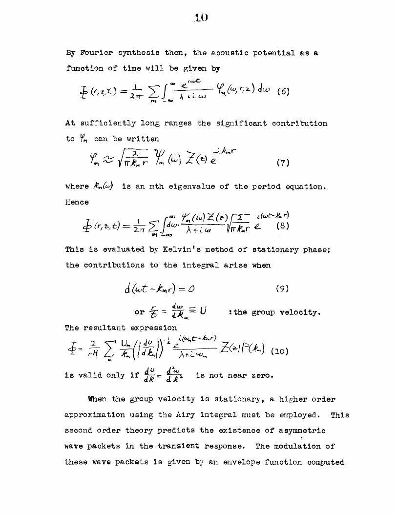
By Fourier synthesis then, the acoustic potential as a

function of time will be given by<wt

At sufficiently long ranges the significant contribution

to can be written

('7)

where ,[w) is an mth eigenvalue of the period equation.

Hence

I~~ irLyz~ r 4a~- (8)() )2At

This is evaluated by Kelvin's method of stationary phase;

the contributions to the integral arise when

t ~41 r) =0 (9)

or :the group velocity.

The resultant expression

)(10)m. Z()- (10

is valid only if s- ' is not near zero.

When the group velocity is stationary, a higher order

approximation using the Airy integral must be employed. This

second order theory predicts the existence of asymmetric

wave packets in the transient response. The modulation of

these wave packets is given by an envelope function computed

by Pekeris, shown in Figure 3. Corresponding to a group

velocity maximum the envelope is reversed in time, giving

a relatively sharp onset. The carrier frequency of an Airy

wave packet is constant, and equals the frequency at the

stationary value of group velocity. Higher approximations

would be necessary if higher derivatives of U were equal to

zero. Although these cases have not been worked out in

detail, we should expect as a check that the higher the

order of stationarity, the sharper would be the onset of

a wave packet at a group velocity maximum.

Applying these remarks to the dispersion curve for a

liquid layer overlying a liquid halfspace of greater sound

velocity, we can deduce, after Pekeris, the form of the

transient signal (Figure 4). If the mode shown constitutes

the main part of the signal, we read this curve as follows.

At = - a small amplitude signal will appear at the

cutoff frequency (As . Following will be a slightly

dispersed train of waves corresponding to the high velocity

branch of the group velocity curve. At it= a high frequency

signal (the direct arrival) will appear superimposed on the

ground wave, corresponding to the high frequency limb of

U. The two frequencies gradually merge into one high

amplitude wave packet at the Airy phase.

Similarly, we can construct a signal from a more

complicated dispersion curve, as found in a three-layered

geometry (Figure 5).

t2

In situations with more than 2 layers, the group velocity

curve has complicated features of the shape sketched in

Figure 5. One or more maxima may occur near velocities

identified with the intermediate layers; the wave packets

generated are interpreted as refraction arrivals from the

top of the corresponding layers. In general, a single

"later arrival" will be composited of several such maxima

from many modes, all arriving more or less simultaneously.

The existence of one or more maxima for some mode will

depend on whether the appropriate layer is thick enough

to support undamped oscillations by itself, in the right

frequency range. Thus thin layers will not produce group

velocity maxima in the lower modes.

Tolstoy, in a series of papers, has outlined a theory

for determination of the dispersion and group velocity in

multilayered liquids. It is the purpose of this paper to

show how this theory can be quickly and easily brought to

bear on problems encountered in seismic refraction studies.

In particular, the person working with seismic refraction

should know, in terms of this theory, how to optimize his

technique and interpretation to get second arrivals. He

should know what frequencies to expect and what modes are

important. The high frequency cutoff of the receiving system

may be critical in this respect, since the higher modes

transmit more detailed information.

Commonly one or more layers may be masked,. i.e. not

13

produce first-arrival information. Accordingly, proper

interpretation of second-arrival information is essential

to the detection of masked layers. In extreme shallow

water situations with shallow bedrock, the nature and

possible thickness of the intermediate sediments can then

be inferred. A recent program carried out in Buzzards Bay,

Massachusetts, by Elizabeth Bunce and the present author 3

presented such problems, and was the motivation for this

investigation. Appendix II contains a description of this

work, with emphasis put on aspects pertinent to the present

paper.

The period equation has been derived in a general way

by Tolstoy 21 , using the idea of generalized reflection

coefficients.

If we consider two liquid halfspaces with a plane

interface (Figure 6), the acoustic amplitude reflection

coefficient for plane waves is given by

(11)

If medium (1) is replaced by an n-layer ensemble, bounded by

a half space, the quantity defined as the complex amplitude

ratio of the wave reflected by the ensemble back into the

(0) region and the incident wave is the generalized reflection

coefficient . 6 can be obtained by summing

14

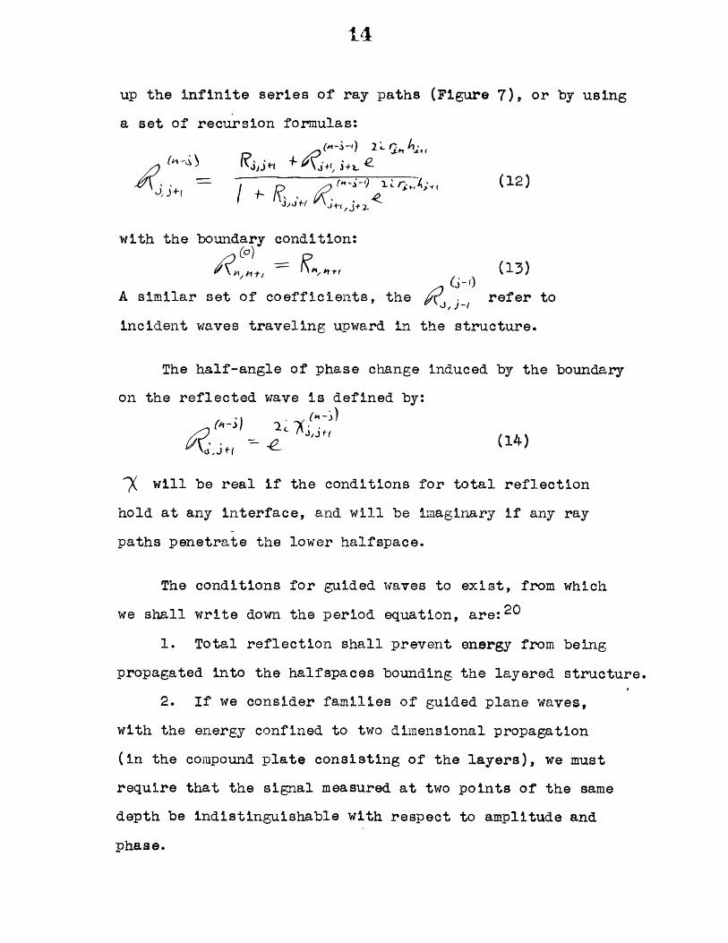
up the infinite series of ray paths (Figure 7), or by using

a set of recursion formulas:

,, +Ir-/(12)

with the boundary condition:(o) _

(13)G-o

A similar set of coefficients, the refer to

incident waves traveling upward in the structure.

The half-angle of phase change induced by the boundary

on the reflected wave is defined by:

(14)

-7 will be real if the conditions for total reflection

hold at any interface, and will be imaginary if any ray

paths penetrate the lower halfspace.

The conditions for guided waves to exist, from which

we shall write down the period equation, are: 2 0

1. Total reflection shall prevent energy from being

propagated into the halfspaces bounding the layered structure.

2. If we consider families of guided plane waves,

with the energy confined to two dimensional propagation

(in the compound plate consisting of the layers), we must

require that the signal measured at two points of the same

depth be indistinguishable with respect to amplitude and

phase.

15

In the situation pictured in Figure 8, then, the period

equation is:

or:

where ff? is the generalized reflection coefficient for

upgoing plane waves incident on the overlying region, and

the other quantities are similarly defined. The integer

m defines the mode number.

Appropriate specialization of Eq.16 provides a system

of equations which define the eigenvalues of the problem.

In terms of an n-layered structure, equation 16 reads:

(Z-0

The recursion formula, equation 12, written in terms of

the phase angles , is:

The boundary condition, equation 13, becomes:

(19

where I, is the imaginary vertical wave number in the

halfspace n + / , so written because total reflection is

assumed at the n - (n i- 1) interface. In terms of guide

phase velocity c, this means:

16

- - ,,.., < ., <C < 0., 1(20)

In general we shall assume that the sound velocity in the

layers increases with depth: C'j < A'j,

If c lies in come other range of values, obvious changes

in certain of the recursion formulas are called for.

Combining equation 17 and equation 18, the period

equation, written in terms of the top layer, becomes:

+tblL 7 tat1 3j= nr (21)

where:

(22)

+ ,r rik +

When total reflection occurs at an interface, j - (j-l),

where j < n, obvious modifications of equation 22 must bemade: r +- ' ' "I.

J-4

( .Jf(

3 (23)

In solving the period equation, if c is used as a trial

parameter, and km is obtained by iteration, a different

modification of the set (22) is necessary for each range

of c used: < C < (a~*

<A < . 1 (24)

In the more general case when q( -Q a1;+, appropriate

modification of (22) is also possible.

The foregoing mathematical scheme was programmed on

an IBM 704 digital computer and used to solve several cases

which are discussed in Chapter III. Further details may be

obtained by consulting the appendices or reference 22.

* * * * * * * * * * * * * * * * * * * * * * * * *

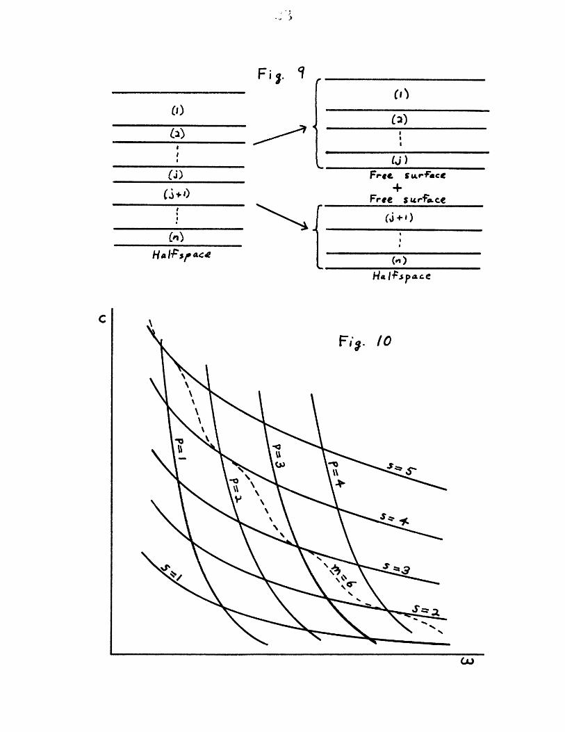
Following Tolstoy2 3, we consider an n-layer system to

be separated along the (Qj +- 1)th interface (Figure 9).

We can write the period equation for each separate wave-

guide:

ij ~ PI~ P' 6 ~~~(25a)

if =s-(25b)'

Each equation will then define a family of curves in the

(4) - C plane which governs the mode propagation for its

particular waveguide. These two families of curves will

intersect to form a lattice of points (Figure 10). Each

lattice point represents a solution to both separated

problems, such that the pressure is a node at the free

surfaces. Hence each lattice point is also a solution to

the original problem, such that the pressure is a node at

the j - (j+1) interface. These lattice points then represent

the subset of solutions to the n layer problem which have

nodes at the j - (j+ 1) interface. We can say that the

lattice points couple the frequencies of the complete

waveguide to those of its components.

18

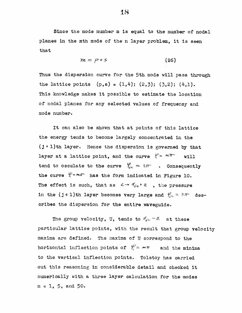
Since the mode number m is equal to the number of nodal

planes in the mth mode of the n layer problem, it is seen

that

M= f+.s (26)

Thus the dispersion curve for the 5th mode will pass through

the lattice points (p,s) = (1,4); (2,3); (3,2); (4,1).

This knowledge makes it possible to estimate the location

of nodal planes for any selected values of frequency and

mode number.

It can also be shown that at points of this lattice

the energy tends to become largely concentrated in the

(j4 l)th layer. Hence the dispersion is governed by that

layer at a lattice point, and the curve m'= -" will

tend to osculate to the curve , == ST . Consequently

the curve f=tr' has the form indicated in Figure 10.

The effect is such, that as C ' , the pressure

in the (j+l)th layer becomes very large and =r' des-

cribes the dispersion for the entire waveguide.

The group velocity, U, tends to der ~2 at these

particular lattice points, with the result that group velocity

maxima are defined. The maxima of U correspond to the

horizontal inflection points of A"7 r and the minima

to the vertical inflection points. Tolstoy has carried

out this reasoning in considerable detail and checked it

numerically with a three layer calculation for the modes

m = 1, 5, and 50.

A_

The J, j + 1 lattice then has the following relation-

ships to the dispersion of the n-layer problem:

1. Lattice points whose indices (p,s) sum to some

particular value m, lie on the mth mode dispersion curve

of the n layer problem.

2. This curve (m) osculates (to a good approximation)

to the curve fg = STE at the lattice point (p,s).

3. Group velocity maxima occur for values of t

defined by the lattice. The group velocity at a maximum

can be estimated by differentiation of the osculating curve

,= S5 at the lattice point.

4. Since p and s define the number of nodal surfaces

for the pressure in the j layer and (n - j) layer problems,

respectively, the lattice enables one to determine by

inspection the distribution of nodal surfaces in the n layer

problem for arbitrary values of the frequency or phase

velocity.

5. Items 2 and 3 depend on the fact that C% +E

These statements hold remarkably well for E. as large as

$. , , and can be used to locate group velocity maxima,

governed by the j + 1 layer, which propagate at velocities

distinctly less than U= 0 +, . Experience will enable

one to regard lattice points in the low modes and at phase

velocities much greater than with the proper caution.

w

Fi. ITypicaI phae.se veloety curves

K

Fig. .Typica l phase velocify c'rves

reverse time scal for.

Iroup velocify maximuI

amplitude(arbi*rary unifs)

Fig. 3Envelepe of the

Airy Phast

4/ Ude=M YWU1

~~1

Fi1 .4

First mode dispersion, groupC veloityj and alpiaude-

Two layers

t= t

A;ry pAase

Fi. 5 Plw)

First mode dispersiont, groupvelocify, and amplitude:

Three. loyer1s

1.0-

0..T-

P(w) I

A;y pAses

u, C.-'

P

U.,,.,

Uc .. 3

-ci.

(w)

1.0 -

P )

gio I Po

(0i)

(i+ /

FE q. 8

I ?lhose~gncous R eglon

Ihi h o m oy vneo usReii

Fi 1. 6

Rey 1071

Fig. 9(I '~)

L~)(I)

Ci)

Halhcspaa:

()Free. Sarf+ce

6+0Free s&r&ae(r'

LH a)~p c

wA

P,

Chapter II

We want to be able to estimate quickly, and with some

accuracy, the group velocity maxima determined by intermediate

layers in a structure, so that the theory will be of some

use in the field and in routine reading and interpretation

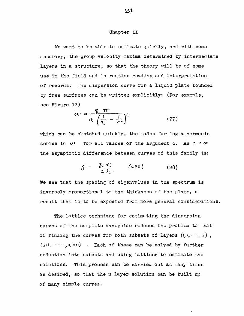
of records. The dispersion curve for a liquid plate bounded

by free surfaces can be written explicitly: (For example,

see Figure 12)

2- Tr .

which can be sketched quickly, the modes forming a harmonic

series in w for all values of the argument c. As c-> oo

the asymptotic difference between curves of this family is:

= (CP-) (28)

We see that the spacing of eigenvalues in the spectrum is

inversely proportional to the thickness of the plate, a

result that is to be expected from more general considerations.

The lattice technique for estimating the dispersion

curves of the complete waveguide reduces the problem to that

of finding the curves for both subsets of layers (IL---j) ,

(+(, -----, , ) . Each of these can be solved by further

reduction into subsets and using lattices to estimate the

solutions. This process can be carried out as many times

as desired, so that the n-layer solution can be built up

of many simple curves.

25

It is possible to consider the n layer problem decomposed

into n - 1 free plates and a plate coupled to a halfspace.

The n separate problems can be used to build up solutions

to the original one by lattices. They should be combined,

step by step, in such a way that the final step involves

the combination of waveguides along the interface j,

j+1, in whose lattice points we are interested.

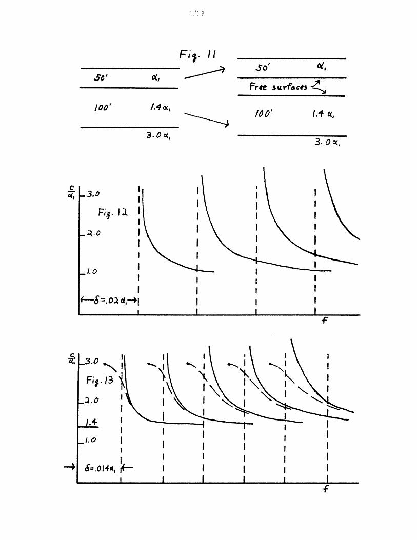
In figure 11 a three layer situation is illustrated.

Figure 12 shows the dispersion curves for the upper plate,

calculated by equation (27). Curves for plate (2) are plotted

in Figure 13, and the appropriate modification is shown by

dotted lines to include the effect of coupling to the half-

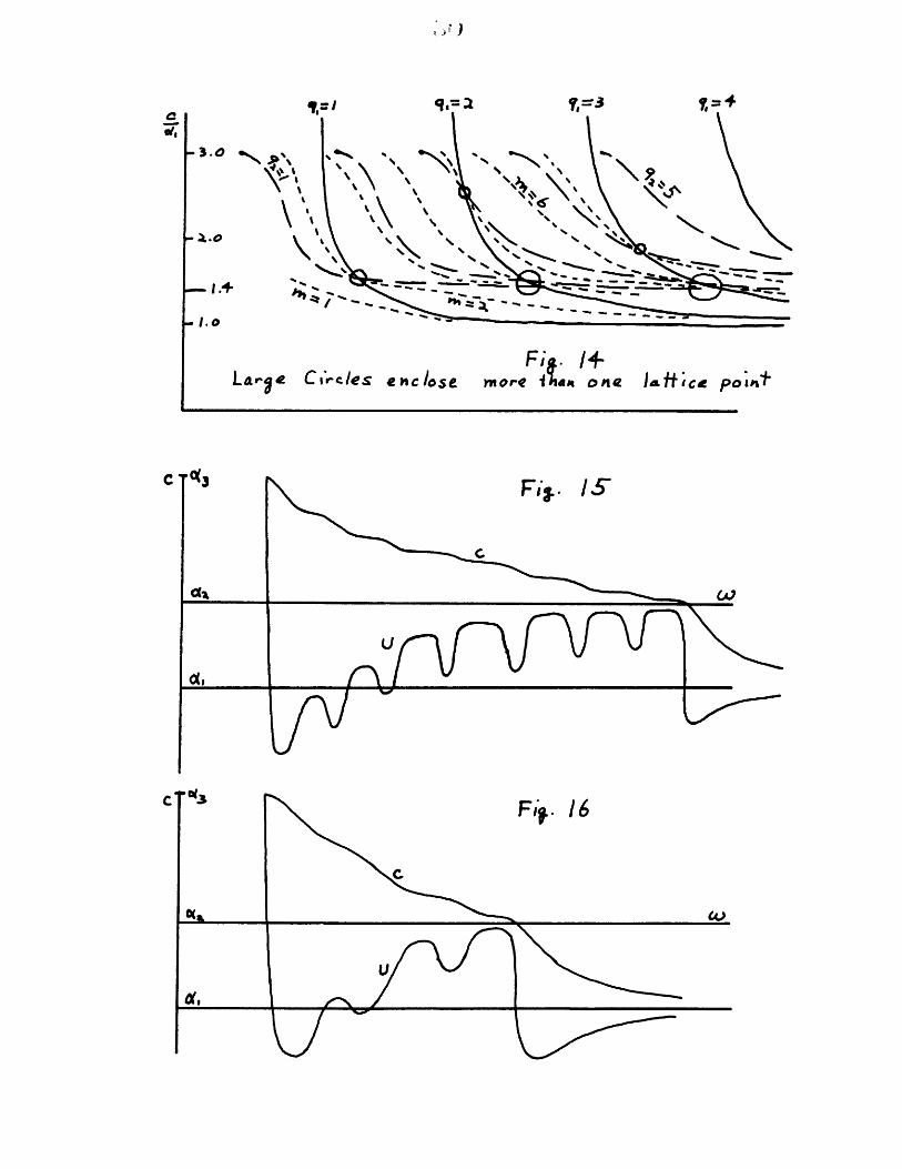
space, (3). Figure 14 shows the result of superimposing

the two families of curves. The lattice points are indicated

and dispersion curves for the 3 layer problem are sketched

in. The lattice points are referred to by their indices

(qi,q 2)- If the lattice were defined by more complicated

ensembles, we would denote their indices by (qij..m prs..v).

This illustration brings out several points predicted

by the theory: 1. The existence of a halfspace coupled to

the waveguide causes a cutoff frequency for each mode

of any subproblem coupled to the halfspace. Thus the

curves for plate (2) had to be modified to account

for this cutoff. For given c, the modification in

F approaches a as c,(>) c>c. , and approaches

zero as C-c4,

2. Where the lattice points are not

sufficiently dense to closely define the dispersion

curve, good qualitative fit can be obtained by noting

that the curve is constrained not to cross curves of

either family defining the lattice except at lattice

points.

3. The asymptotic behavior of the dis-

persion is a help in drawing curves. In this illus-

tration, as C-M, and C< 4. total reflection occurs

at the 1-2 interface and the dispersion is controlled

mostly by the upper layer. Hence the curves m - 1

and qi = 1 agree asymptotically, as do m = 2 and g,

2, etc.

4. The lattice point (;,3) will not

define, even approximately, a group velocity maximum,

since c/<t is almost ~.6 . The remaining points drawn

will define proper maxima: (l -9 andiare so close

to c=Q1 that we can guarantee that the corres-

ponding maxima of U will be very close to L also.

5. The first mode is always ill-defined

by this method. We can estimate its cutoff frequency

by halving that of the second mode; we can plot its

asymptotic agreement with the curve q, = 1.

6. Higher modes tend to have more maxima,

which are closer to C=4 . Figure 5 shows the

possible appearance of a high mode group velocity

curve. The actual disposition of lattice points

responsible for this particular mode controls the

general shape of the phase velocity curve and the gross

behavior of the group velocity curve as it tends from

the lowest Airy minimum to sightly less than C=cd,

The inflections of the phase velocity curve as it

passes through each lattice point are responsible for

the detailed behavior of the group velocity, as it

passes through many maxima and minima. Figure 6

shows a typical group velocity curve for some lower

mode. Naturally, the number of maxima cannot exceed

the mode index.

* * *Z * * * * * * * * * * * *r *

A transient signal will be generated by an infinity

of modes, whose higher order members have very many flat

group velocity maxima, as shown in Figure 5. This makes

possible the achievement of an arbitrarily sharp refracted

pulse, as other considerations demand. This sharp pulse

is known to be due to the discontinuity at the boundary

between layers. Note that if the discontinuities were

smoothed out and continuous variation of the properties

substituted, the effect would be that the group velocity

maxima would not have any limiting property as shown in

Figure 15, but would still exist in similar quantity.

This sort of problem is easily calculated by Tolstoy's

equations and would be a good subject for future investi-

gation.

28

To extend the plate-lattice methods to four layers,

as will be necessary in the next chapter, it is most con-

venient to plot curves for the upper two plates and the

plate-halfspace on one graph. The dispersion curve may be

composited in either order:

(1+ 2) + 3 or 1 + (2 3)

In the former case, the lattice points will give informa-

tion about "refracted" signals along the 2 - 3 interface;

in the latter case they will define refractions along 1 - 2.

Both sets of lattice points will, however, lie on the dis-

persion curve itself.

So' oi100' 4o

Fil. I

.3. 0

Cl I-3.0

Fi. 1.1

-a.0

1.0

C.

-+ 3 .1<

IsoFree sLcrfaces

/001

3. oc~,

I II II II II I

I II II II II I

I j I

I I II II I II I I

I I

I II II II I

)r )

-3.0

-I.0

FiC.etl-Largle Ctire es enclose mnore 1 2^ one lisff ;ce po pnY

C-"'C3 F g.

ofu

v=/.34

t

COLin Fig. 18

Model La+ Lattice poits

e Estimated groupveloc ;+y maximA

+4 ~0

108 ED 0 40cs

F .. 17

directarrivaI

vE 1.0

V~

'.34

I , i:k

200 300106 400 ceps.

Chapter XII

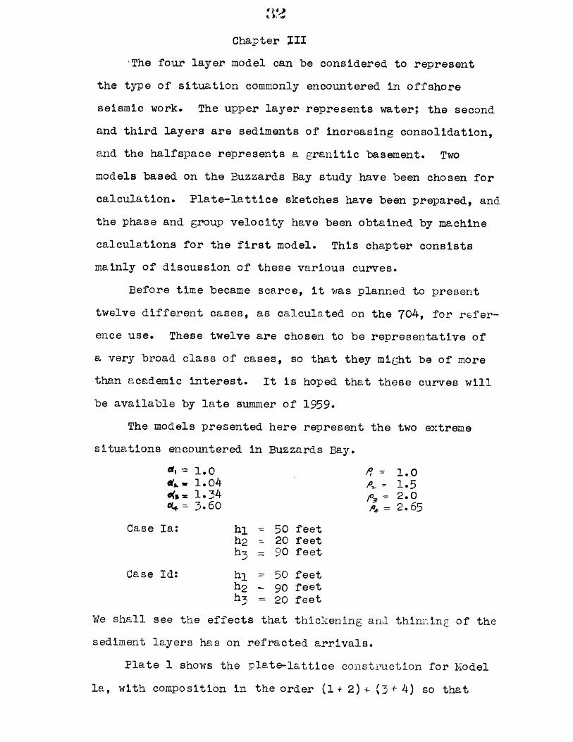
,The four layer model can be considered to represent

the type of situation commonly encountered in offshore

seismic work. The upper layer represents water; the second

and third layers are sediments of increasing consolidation,

and the halfspace represents a granitic basement. Two

models based on the Buzzards Bay study have been chosen for

calculation. Plate-lattice sketches have been prepared, and

the phase and group velocity have been obtained by machine

calculations for the first model. This chapter consists

mainly of discussion of these various curves.

Before time became scarce, it was planned to present

twelve different cases, as calculated on the 704, for refer-

ence use. These twelve are chosen to be representative of

a very broad class of cases, so that they might be of more

than academic interest. It is hoped that these curves will

be available by late summer of 1959.

The models presented here represent the two extreme

situations encountered in Buzzards Bay.

a = 1.0 A 1.0e w 1.04 1.5oo= 1. e34 lo, 2.0c= 3.60 2.65

Case Ia: hl 50 feeth2 20 feeth3 =90 feet

Case Id: hi 50 feeth2 90 feeth3= 20 feet

We shall see the effects that thic1ening and thinning of the

sediment layers has on refracted arrivals.

Plate 1 shows the plate-lattice construction for Model

la, with composition in the order (l+ 2)+ (3 + 4) so that

3

information about arrivals from the 2 - 3 interface is ob-

tained. On Plate 2, to an appropriate scale, the composi-

tion 1 - (2 + (3 - 4) is displayed, yielding predictions on

arrivals from the 1-2 interface. Model Id is similarly con-

sidered in Plates 3 and 4.

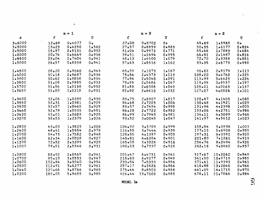
Results obtained from the 704 are tabulated in Appen-case ah/

dix III. Modes 1-12 are considered for beth-ease-; phase

velocity is the independent variable, while frequency and

group velocity are given as dependent variables. Frequency

is also tabulated in dimensionless form as

where H is the total thickness of the finite layers.

Plates 5-8 display the group velocity curves for Model

Ia as obtained from the tables In Appendix III. Phase vel-

ocity curves are omitted for clarity, but these can be eas-

ily obtained from the tables. Lattice points from Plates

1-2 are plotted on Plates 5-8 to afford a comparison of the

approximate and exact methods.

Plates 1-4 illustrate the geometrical factors which

limit the existence of proper lattice points. Most gener-

ally, the thicknesses of both ensembles generating the plotted

set of lattice points control the spacing of group velocity

moxima. In Plate 3, the thinness of the 3rd layer causes an

extreme spread in its spectral spacing, the first mode curve

not approaching 1.34 at all in the range considered. Here

it is imperative that high frequencies be received in order

for the lower layer to be detected. This condition is

34

rectified in Plate 1, as the 3rd layer is quite thick. The

spectrum of this layer is quite dense, and many lattice

points occur at values of c which will generate useful

group velocity maxima. The cross-cutting curves, for layers

(lt 2), now control the spacing of lattice points; were both

layers to be very thin, the wide spacing of curves for (1+ 2)

would create limitations on the existence of useful lattice

points. The same general considerations apply in Plates 2

and 4. In the former, due to the thinness of the upper layer,

we do not expect refraction arrivals at less than about

800 OPs. When this layer is thick, however, the curves q23

become quite dense in the useful frequency band, and useful

lattice points are generated. In Plate 4 the point (q,q 2 3 )-

(2,1) at 350 cps. would give the lowest frequency wave

packet with velocity near 1.04. Note that the control of

the water layer is here manifest; if it were thicker, lattice

points would occur at substantially lower frequencies, poss-

ibly as low as 225 cps.

Another point depicted in Plate 1 is the manner in which

the "plateau" in phase velocity at c=l.34 is more extended

for the higher modes. This plateau represents the attempt

of the phase velocity curve to seek out conditions for mutual

reinforcement of waves traveling in the 1.34 layer. With in-

creasing mode number and frequency, naturally, the range of

frequencies in thich this condition can be nearly met is con-

siderably broadened.

A parameter which is not varied in the figures is the

sound velocity in the sediments. One can, however, visualize

35

the effects very easily. For example, by bringing the

velocity of the upper sediment from 1.04 -il.34, the curves

for q12 are made to cross the 1.34 line more obliquely and

the lattice points are spread out more toward higher fre-

quencies. What is more important is that, is the case (not

depicted) where the two sediment thicknesses are about the

same, the group velocity maxima for the two different re-

fracted events become seriously mixed. Considering the max-

ima one must interpret when only one layer is significant

(for a given useful frequency band) (Plates 5-8), it would

be more difficult to make sense out of signals containing

group velocity maxima controlled by both layers simultan-

eously. In terms of wave dispersion the problem is com-

plicated as follows:: A group velocity maximum pertaining

to the upper of two layers with similar velocities is given

by the existence of a node at its upper surface, hence de-

coupling from the upper layers occurs. Partial decoupling

from the underlying layer occurs when an appreciable vel-

ocity contrast at the lower surface causes only slight pen-

etration by the signal (rj 'rl is large). If the velocity

contrast at this lower surface is only a few percent, pen-

etration of the underlying layer will be great and it will

be a factor in determining the group velocity maxima.asso-

lated with the layer above it. Problems of this sort are

best considered by treating cases of continuous variation

of velocity and density, and noting the effects that the

various space derivatives of velocity have on the dispersion.

Turning to the group velocity curves, one notices that

36

m==2 (Plate 6) has a maximum not predicted by the lattices.

Furthermore, if the 1.34 layer were very thick, we would

have to expect a maximum controlled by this layer even in

the first mode. What this means is that in these low modes,

particularly the first, conditions may not occur for a pres-

sure node at the upper surface of the layer. If the over-

lying layer, having a pressure node at its upper surface,

is very thin, compared to our thick layer, conditions for a

pressure node at the top of the thick layer may be nearly

met. As discussed in Chapter 1, this will tend to cause a

group velocity maximum, more pronounced as the approximation

to a true node becomes better.

In terms of the curves making up the plate-lattice

construction, we may think of the curves for layer 3 as

being very dense due to its thickness, and the curves for

layers (l-2) as being quite sparse. Then the curves for

layer 3 in the low modes will come very close to (but not

contact) the "0" mode curve for layers (l+-2) which is just

the vertical coordinate axis. Thus we do not always have a

lattice point associated with a low mode maximum, but the

virtual contact of the "0" and I mode curves can be thought

of as a quasi-lattice point associated with a first mode max-

imum. It is also reasonable to expect maxima to arise under

various conditions when near contact between plate curves oc-

curs, even though a lattice point is not produced.

Until the intricacies of this machine calculation are

more fully in hand, one must be skeptical of the jagged max-

ima of small amplitude seen on modes 1, 2, and 3. It is my

feeling that the differentiation built into the program may

be inadequate to handle properly some segments of the phase

velocity curve, hence the "bump" in the calculated group vel-

ocity.. These "bumps" will need investigation before they can

be accepted as real.

The curves also point up a matter discussed in the next

chapter; that many group velocity maxima occur at values of

v less than 1.34 (or whatever the layer velocity may be)..

We also see, however, that the high frequency Airy phase for

most modes is very flat and at about U" .9*0o . (Plates 5-8)

This could produce a very strong signal immediately after the

direct arrival, which, due to its broad spectral composition,

would not be in the classical Airy phase form.

While it might be pertinent to make elaborate compar-

isons of the curves with all of the Buzzards Bay records, it

is my feeling that the work would not justify the results.

The records do agree with theory to the order of precision

obtainable by quick calculation with plate-lattice techniques.

At this stage it would be appropriate to carry out more con-

trolled experiments with models to obtain experimental veri-

fication of the theory, rather than just non-contradiction.

-j

I

-J~*JNN pm id -# m4Iim.I4I.DI

p

%mom I 1104WO I - i

-4

.I .. Megalmile shilblelik 4.amed 6412BI whEelimillMmeMinagemmTMtian m.

\ p0

0

0

o

1.04PLATE +1-

Phase Veloc'y for layers1,;1.$ ( 44) ode / .I

S-'~~1

0

N -~ ___ _ ____

0

Maw"..

\ % a

Chapter IV

Attention must now be brought to bear on the appearance

of signals governed by the group velocity considerations

of the preceding chapters. We have seen the effect of the

thickness of layers or ensembles of layers on existence

of the right kind of group velocity maximum for any given

mode. We shall now consider the appearance we should expect

of second arrivals under typical shooting and receiving

conditions.

It commonly happens that the highest modes and fre-

quencies are not evident on a seismic record for several

reasons:

1. The receiving transducer is ofter suspended

at a depth which selects certain modes in preference

to others, a result of the amplitude-depth relation

peculiar to each mode. For example, in the Buzzards

Bay study, receivers hung about 5 feet below the water

surface in 50 feet of water. Basement was about 150

feet deep. The first and second modes were almost

entirely absent from the records. Modes in the range

3 to about 8 were strongly emphasized for most fre-

quencies, while higher mode response would be dependent

in a periodic manner on the frequency. In this instance

ordinary volume attenuation of the high frequencies made

observation of high modes very difficult. Anomalous

instances occurred in which slacking of the receiver

string permitted the transducers to sink to depths

43

where the first mode overpowered other information.

2. Limited high frequency response of the receiving

system will cut out useful high frequency information.

3. Limited resolution (recorder speed) of the

galvanometer camera makes high frequency signals hard

to pick.

* * * * * * * * * _1 * * * *10,-V * * * * * * * * * * *

The more interesting and non-trivial results in this

chapter will apply in situations where volume attenuation

does not remove all the higher modes. The effects described

will be most prominent at ranges such that interaction

occurs between different refracted signals. We furthermore

consider the case where only a few low or medium order

modes are effectively present.

The high frequency components which give the impulsive

onset of a true Fermat least time signal are absent. Search

must be made for wave packets of less distinctive character.

Under certain conditions the time scale will be such that

the interaction between different wave packets will be

slight; in this case picking arrivals is no, problem. At

the other extreme, in the Buzzards Bay investigation, com-

plicated group velocity functions determined a record

shorter than 0.5 seconds. These records were picked by a

brute force technique, to be described, which extracted the

maximum of information and a hopefully low proportion of

random fluctuations. Figure 16 shows the type of time-

distance plot which resulted from this massive picking.

Apparent velocities are signified by v.

In Figure 17 the field bounded by the 1.34 and 3.60

lines contains picks associated with the basement refraction

arrival and its ray path multiples. The field bounded by

the 1.04 and 1.34 lines contains a larger number of picks,

with the following features: Those on the 1.04 line are

high frequency (around 400 cps.) signals associated with

the uppermost sediment layer. The other signals in this

field are not easily distinguished by their frequency from

the ambient signal of the ground wave. However, the 1.34

line forms a distinct envelope to these points. These are

apt to be two linear trends in the points in this field:

1. Lines of apparent velocity 1.04< v < 1.34 inter-

cepting near the.origin.

2. Cross trends with an echelon appearance, having

higher apparent velocities and physically unreasonable

high intercepts. We believe that the echelon structure

(2.) is a result of phase interaction between the signals

associated with the 1.34 layer and the frequencies present

in the first-arrival ground wave. Evidence from a profile

shot in Vineyard Sound where the high velocity sediment

appears as a first arrival at several receivers, strongly

supports this hypothesis.

The envelope nature of the 1.34 line and the linear

45ALit.7

trends (1) of lower velocity are in accord with the group

velocity curves displayed in Chapter III for the extreme

shallow water case. Certain group velocity maxima will

occur at values slightly less than 1.34; others, particularly

at lower frequencies, may occur at distinctly lower values.

The recording system may very well select more of these

spurious lower frequency signals, in favor of the more

significant maxima with apparent velocity near 1.34. Thus

we have the low velocity signals which correlate from trace

to trace, and the fact that none of the arrivals associated

with the 1.34 layer appear prior to the appropriate travel

time.

We might never be sure whether the signals are spurious,

due to low velocity maxima associated with the 1.34 layer,

or genuine, resulting from another layer of lower velocity

overlying the 1.34 material. If the records are closely

spaced, permitting a high density of picks, we are less in

danger of missing some layer by masking than we are of pre-

dicting a layer that does not exist. The paradox is purely

practical; given an optimal receiving system and a lossless

medium we could cause genuine arrivals to have an arbitrarily

sharp pulse front.

Figure 18 illustrates the preceding discussion; lattice

points from case Ia have been transferred from plate I,

where they were obtained, and plotted separately. Corres-

ponding values of the group velocity maximum have then been

46G

estimated by graphical differentiation of the appropriate

osculating curve in plate I. The lattice points which give

rise to the genuine refracted arrival are quite apparent.

A considerable number of group velocity maxima, seem to

occur in the velocity range 1.12 - 1.18, and it would not

be surprising, especially in view of the compressed charac-

ter'of the records, to find strong indications of a refraction

arrival with a velocity around 1.15.

Brute force picking, which is necessary to get the

most information from a visual inspection of a record,

needs some consideration. It is not appropriate, in the

case of a highly complicated set of records, to presume that

information about sediment layers is irretrievably lost in

"noise." Much recent work in seismology has indicated that

virtually all features of a seismic record above the Instru-

mental noise level can be explained by careful application

of theory to perturbations of the original assumed model.

In certain complicated cases, this agreement has been

arrived at by hindsight; reflection records in oil pros-

pecting have been found in close agreement with theoretical

predictions based on a continuous velocity log.5 Tatel and

Tuve19 conducted model experiments where complicated

Rayleigh wave trains known as "ground roll" were generated

by simple surface discontinuities on a solid halfspace.

One is led to hope that similar agreement can be found in

the present problem by modeling; that is, we want to verify

that all the features observed in the field are consequences

of the dispersion of wave trains by relatively simple struc-

tures. If this is not the case, it would be appropriate

to discover how much perturbation of the simple model was

necessary to achieve agreement with actual field seismograms.

The present picking technique will depend only on features

predicted by the available theory. 'When a better under-

standing of all the features found in the field is avail-

able, through systematic crosschecks between model and field

date, there is reason to hope that picking and calculation

of field records can be done with more assurance of relia-

bility.

Given a sequence of seismograms, taken from a receiver

spread, with decent resolution of the significant frequencies,

one sets out to pick all points that seem to represent changes

in the weve train and make a plot in the time-distance plane.

The geometrical relationships which these points display

are the partial basis for deciding on the "reality" of

tentative refraction lines; such geometrical factors will

include not only the existence of linear arrays, but some

of the other features discussed earlier in this chapter.

Since a two-dimensional plot containing a large number of

points will always display "line-ups" of points;'this

matter deserves investigation, namely: given a certain

density of points plotted in a region of the plane, how many

straight line fits of n or more points should be expected

on a statistical basis alone. This additional noise, which

is introduced by the act of plotting points, is another

reason why the geometrical relationships mentioned earlier

should be kept in mind for supporting evidence.

One brute force technique is to plot all peaks

and troughs, filling the plane with I s and -'sl2. If not

enough- traces are available, considerations based on the

theory can be brought to bear, and individual points picked

with some hope of obtaining useful information. Criteria

can be used which tend to select either phase velocities

or group velocities, in trace to trace picking of a spread.

Picking of identical phase points will define a phase velocity;

group velocity is obtained from points of identical frequency.

This latter, the more desirabl.e, is also the more difficult

to apply, unless it is augmented by some arrival of energy

corresponding to a stationary point of group velocity.

To pick an energy arrival, we would require that

the trace have a manifestly higher mean square amplitude

for one or two cycles after the arrival time. One-half

cycle is, of course, insufficient to distinguish the energy

arrival from random fluctuations; one cycle is more meaning-

ful, although interpretation of one-cycle wavelets might prove

difficult, despite their possibly causal nature. Most of the

trace disturbances picked in the Buzzards Bay study were two

cycles or more, except where obvious overlap of signals occurred.

This energy arrival criterion is useful for identifying a

signal; to pick accurately the onset is another matter. If

a distinctly different frequency appears, there is no problem.

4(9

Otherwise one must rely on picking the change of phase

which occurs when a new signal is suddenly superimposed on

the ambient variation. This may be completely successful,

or of no use at all. Failure can occur when the two signals

are entirely in phase, resulting in an indeterminacy of at

least half a cycle in the pick. Signals nearly 1800 out of

phase can produce a null at the true arrival time and a sharp

break part of a cycle later. This is the "echelon" effect

described earlier in this chapter, the delay imposed on the

break being different from trace to trace.

It should not be thought that we would be in dan-

ger of picking a phase velocity and wrongly interpreting it,

since true second arrivals have their phase and group velo-

cities virtually equal. False arrivals would have associated

phase velocities with unreasonable intercepts. It is con-

ceivable that a situation might exist where phase and group

velocities might be read with enough precision to reject

spurious arrivals, although one should not anticipate finding

such a fortuitous occurrence very often.

In a field situation one should apply whatever

knowledge or good guesses are available to estimate by the

plate-lattice technique the frequencies and modes to be

expected in the later arrivals. Hydrophones should be

suspended near an antinode of the important modes and (if

necessary) sufficiently close to the surface to filter out

50

the effect of undesired low modes. The information obtainable

from a sequence of receivers is much more reliable than that

from one receiver; some appropriate scheme is highly desirable.

For example, a floating string of receivers, kept under tow

by the receiving ship, has been used. This string was, in

fact, identical to the array used in shallow water, deep base-

ment reflection prospecting for oil. When more conventional

equipment is available, an array can be improvised; depending

on the length of the vessel, buoy-slacked hydrophones may be

established at intervals from bow to stern, no less than about

40 feet apart, and at the desired depth.

For receiving equipment, a broad-band amplifier, such

as the Woods Hole "suitcase" is recommended, feeding into

two or three filtered channels for each input. A multichannel

galvanometer camera with appropriate paper speed and galvano-

meter resonance is the best recording device for eventual

visual interpretation. The hope is that one or two trial

shots would be sufficient to optimize the filter settings.

Normally on a multichannel re.cording, one low frequency trace

is used to obtain deepest penetration; one high frequency

trace is needed to get an accurate time for the direct

arrival. We would be interested in peaking the other

channels at the frequencies of the later arrivals.

The existence of a receiving array should make it

possible to extract signals from hydrophone noise by corre-

lation techniques. The possibility of establishing such a

method with present FM tape recorders should not be over-

looked. Experimental use of a frequency analyzer, such as

the "Vibralyzer", when tape recording is available, is

strongly suggested. Vibrograms taken in a sound transmission

study of Buzzards Bay showed unquestionable evidence of

bottom sediment refracted arrivals. These agreed closely

with the frequencies observed in the ralvanometer camera

recordinEs which constituted the main body of the Buzzards

Bay data.

While transmission of energy in the waveguide occurs in

the various modes, losses can occur in these "undamped"

modes by frequency dependent volume scattering, particularly

in the sediment layers. If this mechanism is significant,

the signal received at the hydrophone will already be

filtered. Since these losses are primarily in the higher

frequencies, the signal to noise ratio is adversely affected

in these useful frequencies. In a highly lossless situation,

there is much to be gained by running at least one high fre-

quency broadband channel, to obtain the effect of as many

significant group velocity maxima as possible. If the shot

distance is great enough or the sediment thickness sufficient,

the high frequency signals will be attenuated and an unfavorable

signal to noise ratio ensue. It would then be advisable to

record narrow band channels sufficiently below the center

of the noise spectrum in an attempt to get wave packets from

individual group velocity maxima. The problem in low mode

broad band recording is that severe amplitude contrasts may

exist between neighboring modes; our attempt to put all the

eggs in one basket by broad band recording is apt to show

only the strongly excited modes and render unreadable the

wave packets of interest.

Tolstoy 4, in a test of his theory, employed measure-

ments with a constant frequency source and a calibrated

hydrophone, taking the mode interaction wavelength as an

easily measured quantity. This is a promising new technique;

we are here interested, however, in conditions for observa-

tion of transients, and mention this only for the sake of

completeness.

* * * * * * * * * * * * * * * * * * * * * * * * *

It is appropriate to ask what effect slight variations

in the layer thicknesses might have on the refracted signals.

From geological considerations it is often possible to estim-

ate how well or how poorly the earth materials under consid-

eration approximate to a plane waveguide. One would want to

know what fundamental limitations the expected perturbations

in the geometry would impose on the detection of arrivals.

It should be noted that the other types of departure from

the ideal model will not be considered. Seldom do inhomo-

geneities in the layers reach the order of a wavelength in

size. The existence of smooth, rather than discontinuous,

variation of the physical parameters at a boundary is a pro-

blem deserving separate consideration. The geometrical

53

factors involved in perturbation of a boundary can be

interpreted with the use of the plate-lattice analysis,

hence we shall devote a few paragraphs to it. A through

mathematical analysis will not be attempted, since a really

useful and concise formulation of the unperturbed solution

is not available yet.

We assume that the sediment layers have variable

thickness over the range of a given shot. This amounts to

a sequence of perturbations which are imposed in a certain

order on the normal modes. For this discussion the pertur-

bations will be considered to be one-dimensional:Le. linear

structures at right angles to the direction of propagation.

Any effect these perturbations have on wave character will

be a limiting maximum to the effects we would expect from

the physically more reasonable case of two-dimensional per-

turbations. Following usual practice we consider the two

limiting types of perturbation: adiabatic and sudden.

In the adiabatic case, with the four layer models in

mind, the interface between the second and third layers

will be considered to vary gradually over a long range.

Such a situation occurs on the continental shelf where

relatively homogeneous layers thicken toward the edge of

the shelf. Parallel to the structure, less systematic

variation of the sediment thicknesses takes place, but in

the same gradual manner. Mathematically, this is a limiting

a4

case of the well-known "wedge" problem, which is insoluble

by standard eigenfunction techniques. We consider an unper-

turbed region propagating mth mode plane waves (distant from

the source). If the modes of this problem are nearly

orthogonal, or if an orthogonal set can be found by change

of variable, the perturbed problem would be solved by the

mth mode of the perturbed geometry: i.e. in the adiabatic

approximation no transitions occur between modes (states).

This type of situation would tend to preserve the character

of a refracted arrival; naturally the high modes would be

the first to suffer, but it is so seldom that we receive

the sharp, high frequency edge of the pulse, due to other

factors, that this is not a fundamental limitation. As long

as the local slope of an interface on the continental shelf

is as low as 1:50, the usual situation, modes 1 through 10,

which will probably contribute the refracted signals, will

propagate with the same weights in the perturbed waveguide.

This analysis predicts a set of group velocity maxima in

the perturbed geometry with the same number and character as

in the unperturbed situation. Hence, the prediction results

that the refracted arrivals will propagate with the same

apparent velocity as before. The anticipated prediction,

that some change in the apparent velocity will occur, due

to the slope, is not possible using the present mathematical

description. It does not "see" time differences due to

variations in the geometry, because the group velocity --

waveguide description is equipped to synthesize pulses only

in the horizontal direction.

Naturally, if the layer thickness is perturbed suddenly,

transitions will take place between modes; the transition

amplitudes will be proportional to the vector inner product

of the mth mode of the unperturbed problem and the nth mode

of the perturbed problem. Such a situation was encountered

in the Buzzards Bay study; with the aid of a "sparker",

graphical reflection records of the sediment were obtained,

showing homogeneous bottom sediment overlying glacial drift

with a very irregular upper surface. Here we would expect

the mth mode signal at the receiver to be due to a series

of transitions, appropriately summed. A discontinuously

"sudden" perturbation would also induce a reflected wave

in the -r direction. This could attenuate refracted

signals more than any mode transitions. Under less

stringent conditions, more sensible physically, the per-

turbation might be sudden enough to induce mode transitions

yet not have the discontinuity necessary to generate an

appreciable reflection.

In cases where the perturbation of an interface has

very restricted range, but the least bound on the derivatives

is very large, the modes will be slightly less well defined,

but the unperturbed modes will still give a good representa-

tion of the dispersion. The rough surfaces will permit

energy to be radiated into the bottom, effectively increasing

56

the range attentuation factor. Scattering from rough sur-

faces is a well-known problem in acoustics, and a straight-

forward application to this problem should present no diffi-

culties.

Qualitatively we can sum up the effects these mechanisms

will have on the significant wave packets composing a re-

fraction arrival. The smearing of the spectral curves by

rough boundaries will tend to destroy the critical phase

relationships among the different wave packets arriving

close to time , and thus tend to blunt the rise of

the pulse. This is mentioned only in passing, because the

customary attenuation of high frequencies in a real structure

more effectively filters the whole transient. If all modes

are received, perturbations in any of the boundaries will

change only the frequencies of the component wave packets;

their transient sum, which is the observed signal, will

retain its sharp pulse front. In practice, however, the

usual factors will cause the observed signal to be composed

from a band of frequencies (usually less than one decade).

Any perturbation which will seriously change the number of

useful lattice points in this band will threaten the integrity

of the pertinent refraction arrival. This is a problem

when thin layers are present; the lattice points contributing

to the refracted arrival may be only one or two in number.

Furthermore the inverse h dependence of the spectrum for

single layers makes these lattice points exceedingly sensi-

57

tive to perturbation of h. Thus a small perturbation may

modify the refraction arrival from a thin layer quite pro-

foundly. It is conceivable that in such situations the

one or two wave packets would be thoroughly disguised;

information would still be present, but would have to be

extracted by more sophisticated frequency analysis.

Example Ia has several lattice points in the effective

band of, say, 100 to 500 cycles. Here we should expect no

trouble in receiving second arrivals if some perturbations

were to occur, since sufficiently many lattice points of

the perturbed problem would fall in the right band. The

effect of many mode transitions, due to a series of per-

turbations in the shot-receiver interval would be sliEht in

this instance. This is because the part of the observed

signal due to modes is due only to the modes of that part

of the waveguide local to the receiver, and we have indicated

the acceptability of lattice points in these modes. If a

series of transitions has occurred, two other effects

are apt to reduce the amplitude of the wave packets:

1. The probability of back reflection, previously

mentioned, if the perturbrtions are sharp enough.

2. Broadening of the range of modes originally

the explosive source favored a certain wide range of

modes; i.e. the source spectrum always determines the

relative excitation of different frequencies. A series

of mode transitions may excite modes outside of the

originally significant range, hence the relative

excitation of the few observed modes must decrease.

This cannot mean that new frequencies are introduced;

it is the wave numbers and phase velocities that change,

subject to the period equation.

It is now apparent, in general, that we must expect

more difficulties in observing refraction arrivals when

geometries with perturbed layers are considered. In a

great many cases, however, much or most of the useful

information is retained in the signal. The need for

mathematical investigation is apparent, and many possibilities

for this have been suggested.

59

Conclusions

The plate-lattice analysis enables one to obtain use-

ful information about the transient 4ignal and, particularly,

the refraction arrivals from layers above the basement.

Information of a sepqtral nature, such as the central fre-

quencies of the wave-packets, is easily come by.. The

phenomena of interaction between a second and first arrival

and the existence of group velocity maxima with spurious

velocities are of the same type. As remarked before analysis

into modes makes possible synthesis of a transient signal

traveling in the r direction only. However, in order to

rigorously account for second-arrival transients, the theory

must incorporate travel times in the overlying layers. The

approximations inherent in the present work imply a zero

intercept for the refraction lines. Thus, we have learned

a good deal about the refracted arrivals insofar as fre-

quency is concerned, particularly since the recording system

and transmitting medium act as a bandpass filter; we have

not yet accounted for intercepts and changes in apparent

velocity due to slight perturbations in layer thickness.

A complete theory would be desirable which handled refraction

arrivals from upper layers at short ranges, indeed, in cases

where they occur as first arrivals.

Press1 6 has suggested that an expansion of the inte-

grand of the formal integral solution could be performed

which would give a fairly concise expression for the phenomenon

O0

of interest. I have not given the matter much consideration

beyond this, but I feel it very unlikely that any attempt

to mathematically sum all the contributions from group

velocity maxima would meet with success, especially in

view of the limitations expressed above. Beside involving

complicated double sums of functions like the reverse Airy

phase, this would always leave considerable doubt about

the physical meaning of the answer. For the time being

we must be content with knowing that the main body of a

refracted pulse comes from the group velocity maxima and

that useful knowledge about the frequencies present is

readily available from the same theory.

61

Appendix I

Table of Symbols

compressional wave velocity in the ith layer

thickness of the ith layer

. density of the ith layer

vertical coordinate

r horizontal coordinate

C horizontal phase velocity

CU angular frequency

F frequency= b* horizontal wave number

vertical wave number in ith layer= -

imaginary vertical wave number-

U group velocity -

V any apparent velocity

t time

m mode index for entire waveguide

mode index for waveguide consisting oflayers: 1, J, ...

generalized Rayleigh reflection coefficientfor layers ( +1, j+ 2, ... ,n), jbeing the medium of incidende.

Rayleigh reflection coefficient at the j,j + 1 interface,, j being the medium ofincidence.

half angle of phase change induced by reflectionat the J, J+ 1 interface in the waveguide.

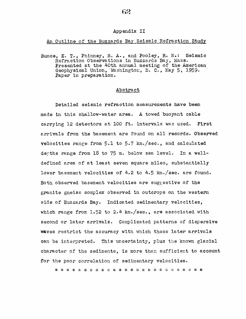
Appendix II

An Outline of the Buzzards Bay Seismic Refraction Study

Bunce, E. T., Phinney, R. A., and Pooley, R. N.: SeismicRefraction Observations in Buzzards Bay, Mass.Presented at the 40th annual meeting of the AmericanGeophysical Union, Washington, D. C., May 5, 1959.Paper in preparation.

Abstract

Detailed seismic refraction measurements have been

made in this shallow-water area. A towed buoyant cable

carrying 12 detectors at 100 ft. intervals was used. First

arrivals from the basement are found on all records. Observed

velocities range from 5.1 to 5.7 km./sec., and calculated

depths range from 18 to 75 m. below sea level. In a well-

defined area of at least seven square miles, substantially

lower basement velocities of 4.2 to 4.5 km./sec. are found.

Both observed basement velocities are suggestive of the

granite gneiss complex observed in outcrops on the western

side of Buzzards Bay. Indicated sedimentary velocities,

which range from 1.52 to 2.4 km./sec., are associated with

second or later arrivals. Complicated patterns of dispersive

waves restrict the accuracy with which these later arrivals

can be interpreted. This uncertainty, plus the known glacial

character of the sediments, is more than sufficient to account

for the poor correlation of sedimentary velocities.

G3

Comments

This study, which was started in the summer of my

Junior year, has been for me a complete course in record

reading, instrumentation, end theory. It appears that

the records obtained were unique in reftactiontwQrk, for-the

short time and distance scales involved. The departure of

the sediment-sediment interface from a plane also must

have set some kind of a record for our presumptuousness

in trying to "shoot" it by refraction.

The presently available results from the Buzzards Bay

study involve delineation of the basement topography, and it

was with some confidence that we were able to present pro-

files of the basement surface. Although our knowledge of

the sediments was less than unique, we felt that we had

achieved some intimacy with them after reading over 200

high quality records for sediment arrivals. Several

features appeared in the plots which repeated from profile

to profile and seemed to warrant looking into. This be-

havior of the plotted points is explained in Chapter IV of

this thesis. One can imagine, for example, our initial

surprise when the first good record obtained showed good

correlation of a wave packet on four adjacent traces, with

velocity around 10,000 ft./sec. and a time intercept four

times greater than the intercept from the crystalline base-

ment.

A couple of fortuitous bits of data not included in

(4

the original program proved to be of real value in pinning

down these sediments. After a couple of tries, a usable

sparker record was obtained which showed without question

the structure of the sediments: A fine grdned homogeneous

clay or silt which formed the flat bottom of the Bay

overlay, across a very irregular interface, material which

scattered the sound so distinctively that its glacial

character was considered proven. The basement, only a

few fathoms beneath the drift, was not seen at all on the

sparker records due to this excessive scattering. Because

of the shallow depth to basement and noting the important

role glaciation played in the area, we feel that the drift

directly overlies the basement. We were also fortunate in

receiving from Dr. Charles B. Officer, Jr., records which

were shot in Vineyard Sound, only about 3 miles southwest

of some of the Buzzards Bay work. When these were plotted,

the structure of the sediment was made obvious, due to first-

arrival date, and the envelope nature of the second arrival

part of the high velocity sediment line was explicited.

Another feature we found, which was to be explained by

the Tolstoy theory, was the occurence of a physically

unbelievable number of good sediment refraction lines.

It now appears that only the greatest and the least of these

were real, corresponding to the two sediments just mentioned,

while all the others were due to group velocity maxima

governed by the higher velocity layer. One record showed

this feature remarkably well; no less than six sediment

65

layers seemed to lie in a 100 foot vertical interval.

Needless to say, the method of pickine signals, which

is discussed in Chapter IV, was not laid out after shrewd

consideration of the present theory. It was, however,

soundly based on the fundamentals of the way energy travels

in a wave, and has to make some kind of sense in terms of

any reasonable theory. We were gratified that the time-

distance plots did not look like scatter diagrams, but

that certain features stood out on a large number of

shots. The present thesis was undertaken in an effort to

understand these features and learn more about the nature

of mode propagation.

m=2

12.6913.2315.9720.7623.0426.57

28.2030.1830.6231.0831.5631.80

32.0632.3132.573207933.0138.53

3.60003.50002.50001.80001.65001.5000

1.45001.40001.39001.38001.37001.3650

1.36001.35501.35001.34601.34201.3200

1.28001.24001.20001.16001.12001.1000

1.08001.07001.06001.05001.04401.0200

0.40770.42500.51310.66690.74040.8538

0.90600.96970,98380.99851.01381.0218

1.02991.03811.04651.05351#06051. 2379

1.38251.55541.75822.00282.32992.5546

2&85693.05533.30403.62773.87665.9455

0.87020.88590.99721.26941.45001.8516

2.10732.43732.50402.56862.63082.6610

0.1.5620.9320.9360.9410.941

0.9430.9360.9340.9330.9320.931

0.9300.9290.9290.9510.9251.026

1.0060.9780.9480.9270.9250.931

0.9410.9470.9540.9610.9650.985

27,0827.5731.0439.5145.1357.63

65.5975.8677.9479.9581.8882.82

83.7584.6885.5786.2886.9993.52

104.92116.55128.85143.81165.05180.33

201.47215.63233.54257.17275.46426.44

MODEL Ia

0.0.9850.7710.9951.0791.162

1.1671.1131.0911.0671.0431.032

1.0171.0060.9980.9820.9811.047

999939905901916928

0.9410.9490.9560.9640.9680.985

49.6950.3555.6666.9172.7083.35

90.82108.20113.99119.95125.01127.07

128.87130.48131.96133.06134.11141.97

158.54177.13197.31221.80256.76282.18

317.67341.50371.61410.98441.09678.11

1.59651.61771.78832.14972.33582.6779

2.91793*47623.66253.85374.01634.0826

4.14054.19214.23984.27514.30894.5612

5.09365.69086.33917.12618.24949.0660

10.206210.971911.939313.204014.171521.7866

.6907

.7205o7494.7722.7949.0045

3.37093.74444.13974.62045.30285.7937

6.47316.92777.50338.26268.8502

13.7008

434854627279

8895

102112120185

.03

.41

.73

.34

.52

.51

.92

.10

.84

.91

.66

.05

0.0.8240.6840.8160.8810.998

.113s225.224.197.137.101

1.0651.0291*0050.9860.9661.023

1.0030.9550.9200.9130.9260.937

0*9490.9550.9610.9660.9700.984

m=3m=1

m=4

3.60003.50002*50001.80001.65001.5000

1.45001.40001.39001.38001.37001.3650

1.36001.35501.35001.34601.34201.3200

1.28001.24001.20001.16001.12001.1000

1.08001.07001.06001.05001.04401.0200

67.3368.0374.6291.29

100.93116.15

123.05134.16138.98147.35162.30172.43

181.02185.39187.78189.22190.45197.73

212.95231.80255 i 14286.02332.82368.72

421.86459.17506.61566.28609.69930.74

2.16332.18582.39752.93293a24283.7316

3.95354.31034,46534 s73415,21465.5401

5,81595,95646&03316,07946*11906.3526

6.84187.44758.19729.1894

10,692911.8464

13,553814,752516,276518,193619,588529.9032

0,0,7120.6780*8960,9380,919

0,9411,116161951,2581,2891,286

1.2351,111069990,9760,9080.917

009190*9120.9070.9140*9360.951

0,9650,9710.9720.9710i9720,983

87.0187*7194.56

111013121.76148.82

166.51180.39182.81185*47189#36193,60

204s63226.80244*70248*43250.48259*73

277*21297.56322.71356,58408*03447,29

507.02553.32622.77718,37779.11

1183.45

MODEL Ia

2,79542.81793,03813#57053491184.7813

5.34985,79575*87335,95886.08376.2202

6.57467.28697#86187,98178o04778*3446

8.90639o5601

10,368111.456213.109414,3708

16.289717,777420,008723,080225.031538.0226

005950.5830.8110.9511,136

1,0940.9060.9010,9471.0961.224

1.2991.3131.2171.0430a9610.894

0.8750.8670.8720.8890.9180.937

0,9630,978009910.9830.9740.982

105.03106.02116.50142.90155.26172.46

185,66226.44234*71240.02244.11246.15

248.58253,51279.47297,83302.04315.42

339o56365,98397o14438.20499.26544.17

608,00653o24720.12855.43948.26

1436.17

3.37453#40623* 7 4 3 04o59124.98815,5410

5.96507,27527,54087.71157.84287.9085

7.98668.14498s97899,56889.7042

10,1340

10.909411.758512,759714,078816s040317.4835

19,534120# 9 8 7 823,136427.483630.466146,1421

0.0.6840.6980.8950.8170*886

.127

.204

.109.994.943i957

1.0311.2211,316120410410.936

0.9000.8740.8700*8850.9100.925

0.9440.9580.9831o0040.9790.982

=5 m=6

m= 8

3.60003,50002.50001.80001.65001. 5000

1,45001.40001.39001.38001.37001.3650

1.36001.35501.35001.34601.34201.3200

1.28001.24001.20001.16001.12001.1000

1.08001.07001.06001.05001.044010200

127.51128.22136.96158.99176.04215.00

229.02248.34260.84278.10290.30294.06

297.34300.91309.99344.93351.32364.55

391.49424.32464.02515.90592.14647,38

723.57774.61841.28962.98

1115.711688#89

4.09664.11954,40025.10825.65606,9077

7.35817.97888.38038.93499.32719.4478

9.55309.66779.9594

11.082111.287511.7124

12.578013.632914,908316.575119.024720,7993

23,247224,887127,029030.939035.846254,2616

00.4820.5460.8251.0111,028

049051s1661,2431#23011001a039

1.0161,0711.2761.2881,0160.904

0,9090,8970.8900.8980.9170,928

0,9410,9500,9631,0070,9890.982

142*7114383157o43192.03207,57235,59

26239288s83294.80306.11330.61339,57

344,10347.43351.33379.10410.27423.00

448.42480,39521.95579.92670.93740,53

837o5890039977,60

1086#451277#391941.61

MODEL Ia

4,58504s62115.05796.16966,66917s5690

8*43029*27979*47149s8349

10,622010*9099

11,055411.162511*287612#180013,181513s5903

14,407115.434116*769418,632021.556123s7920

26,910328,928131.408934,905941.040562,3811

0.0.6210 6890.8290,8021.062

1.129009981.0761.2221.2501.138

1,0120,9701.0881.3271.0060.846

0*8560.8670*8810.9030.9310#944

0.9510.9530.9580.9831.0080.981

166o96167.92179.91210.11232*24269,03

288.55331.07336.42341.96354628374.27

397,78404,50407.90412.34468,76484.61

513.40547.63591.04650.88744.01817.55

933.361016.861115.251234.421417.562194.33

5,36415.39505*78016s75047.46148s6437

9 t270610,636710,808810*986611 o382512,0248

12,780012*995913.105313.248015.060515,5699

16.494917,5945184989320.911723*903826,2667

29,987432.670335.831339.660045.544070.5006

0.0.5010.5450.8410,9840.927

1.0900*9960&9440.9951,2411,296

1.2370*9870.925101931,1470*855

0.8440.846018600.8850.9190.943

0,9670.9700.9640,9691.02400981

m=9

=m=12

203.16204.26219.29261.94286.90324.58

6.52736.56257.04548.41579.2176

10.4282

Oil0.49105780.8780.8481.061

c3.60003.50002.50001.80001.65001.5000

1.45001.40001.39001.38001.37001.3650

1.36001.35501.35001.34601.34201.3200

1.28001.24001.20001.16001.12001.1000

1.08001.07001.06001.05001.04401.0200

f182.53183.68199.08237.01256.49303.62

322.56367.22386.59395.49401.32405.26

420.72456.48465.34469.26517.26537.55

573.64615.07665.33732.59833.50908.63

1020.461109.841242.831389.021530.102447.05

m = 10

5.86445.90136.39627.61478.24079.7550

10.363311.798112.420512.706512s893813.0205

13.517014.666014.950715.076516.618717.2708

18.430419.761221.376123.537226.779129.1928

32.785835.657639.930344.627149.159978.6201

U0.0.5390.6370.7840.8741.021

0.9031.2451.1650.9460.9291o068

1.2951.2611.0011.0401.2550.892

0.87408600.8630.8820.9090.927

0.9550.9770.9810.9671.0170.981

222.67224.07242.51282.05307.70364.40

7.15427.19907.79149.06189.8861

11.7077

384.16 12#3 4 25444.63 14.2853451.61 14s5095462.73 14* 8 6 7 0495.76 15o9279504.98 16.2244

510s68518.79562.07568.63627.26648.49

684.30729.41788.98873.83

1008.831109.96

1245*491333s611451.971694.161831.572952.49

16.407516.667818.05831 8 s2 6 9220.153020@8351

21.985523s434825s348828*074932s41 2 335.6613

40.015742*846946#649754.430958.845594*8591

MODEL Ia

394.13407.26437.75455.67459.90

464.62483.59512.34517.72569*19588.10

624.81671.41730.55809.99927.16

1011s57

1128.881211.491344.081544.041669.982699.77

12.662813* 0 8 4 6

14. 0 6 4 314s64 0 114* 7 7 5 9

14.927515.537116. 4 6 0616* 6 33618o287318.8949

20.074321.57132 3# 4 7 1426*023829.788332.5003

3 6 s 2 6 9 4

38.923443.183349.607753.65418 6 s 7 3 9 6

364.79 11 7 2 0 3 1s14409971i2291i2541.015Os966

1.0571s300is1291s03210313Os852

0.870087608810s8940Os9130925

09420s9580.991Os9720.9930.981

0.0.5420.6090.7450.9870.855

1.0480.9720.9621i1751.2151.066

1.0141.1921.2470.9541i3320.821

0.833O.8490s8710.899O.9280.937

0.9430.9490.9710.98709780.981

m=11

~; k()

U/d,

E07

07

PLATEModel Ia Grocup Ve/~cify

200-1 0'F (cgs)

Os-

J.5

I.34

l.0

m=5m=I

0.5

5

400 500

06

rn=JO

0'

PLATEModel . :

6

Group Weiocity

S(cps)- 1007~~~ -304050

U/dt,

'.5

J.0

o.s

Y00300 400

1.5

/.0

05

OsY

C7

PLATE 7Model a. Geocip Velocity

- 76O~

I40 300

f (c p S)

07

||I

400 S-00

I

n

Aa-7

738

=4.

Os

I hi 0-~

- -~ ~ -

I -~----------_

IM =JIa

so-_8-.Q

f- (cps)300

'S

'34

1.0F-

0.5~*

0 - p

8PLATEModel 14a :

400 400

j

Imm"

U/Olt

0

G(A h />C I ty

APPENDIX IV

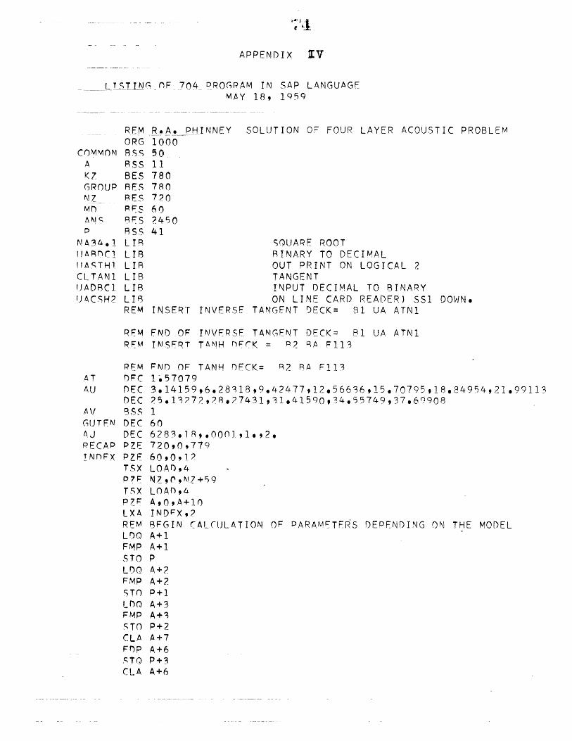
LESTING OF 704 DROGRAM IN SAP LANGUAGEMAY 18, 1959

RFM R.A. PHINNEY SOLUTION' OF FOUR LAYER ACOUSTIC PROBLEMORG 1000

COMMON RSS 50A BSS 11K7 BES 780GROUP RES 780NZ RES 720MD RES 60ANc RFS 2450

R SS 41NA3l.1 LIR SQUARE ROOTUARC1 LIB RINARY TO DECIMALIASTHl LIR OUT PRINT ON LOGICAL 2CLTAN1 LIB TANGENTUADRC1 LIB INPUT DECIMAL TO BINARYUACSH? LIR ON LINE CARD READER) SS1 DOWN.

REM INSERT INVERSE TANGENT DECK= Bl UA ATN1

REM END OF INVERSE TANGENT DECK= Bl UA ATN1REM INSERT TANH r)CK = R2 RA F113

REM END OF TANH DECK= R2 RA F113AT DFC 1~.57079AU DEC 3.14159,6.28318,9.42477,12.56636,15.70795,18.84954,21.99113

DEC 25.13272,28.27431,31.41590,34.55749,37.69908'AV BSS 1GUTEN DEC 60AJ DEC 6283.18,.0001,1.,2.RECAP PZE 720,0,779TNDFX PZE 60,0,12

TSX LOAD,4P7F N7,0,N?+59TSX LOAD,4PZE A,0,A+10LXA INDFX,2REM BFGIN CALCULATION OF PARAMETERS DEPENDING ON THE MODELLOO A+1FMP A+1STO PLDO A+?FMP A+2STO P+1LDO A+3FMP A+3STO P+2CLA A+7FDP A+6STO P+3CLA A+6

Z3

FDP A+5STQ P+4CLA A+5Ff)P A+4STO P+5CLA A+8

FDP A+10STO P+6CLA A+9FDP A+1 STO

_ CLA

FDPSTO(LAF)PSTO

FDPSTOREM

DHA LXDL DO

FDPSTOFDP'; TOQCLAFSRTSXNOPCHSSTOCL AFDPSTOCLAF SRTMIR EMTSXNoPTRA

L IMP0 CHST;XNOPCHS

GABRO STOCLAFDPSTO(LAFS PTMITSX

P+7

P+9A+9

P+10A+10

P +1 1REGIN CALCULATION OF PARAMETERS DEPENDING ON PHASE VELOCITYINDEX ,1Mr),2Mr, 2CRAMR+1P+12P+2P+13A 3+2P+13SORT,4

TAG A4P+1?P+12p+1P+14P+14AJ+2LIMBO9FGINNIN; OF PAGF 4SORT,4

GARRO0

SPT ,4

Pp + 1~ Ll

P+15P+15A J+2LIMBCSOPT ,4

TAG A3

---I

NOPTRA

LIMRC CHSTSXNOPCHS

PARA ST rCLAFS RTSXNOPSTOLDOFMPFDPREMSTOL r)0FMPSTOLrGFMPS TOCLATPLCLATPLTRA

CPPCS FADSO1PS FAD

TRASLURP CLASLUMP STO

FDPSTOTRADECCLAFDPSTOCLA5SPFDPFMDSTOSTZCLAFDP

CLASSPFDPFMPSTO

GARRA

SOPT ,4

P+15P+12AJ+?SORT,4

TAG A2

AUTOMATIC ERROR CHECKP+16

P+11MD,2BEGINP+17P+16P+6P+18P+IlP+7P+19P+14SPECSP4-19SOUPSSLURPP+19P+18SLUMPP+18P+20SLUMP+4P+28*+2.25A+6P+14P+21P+21

PAGE 5

0 TAGGED

CHECK TAG OF A3

A+5P+15P+21P+23A+5P+15P+22P+22

A+4P+16P+22

FDP P+13STO P+23CLA P+?3SSPFDP A+6FMP P+14S_ _ P+23

HOBOR TPL PAULREM LOOP IN NEW MCLA P+21TPL PAULCLA P+22

PAtIL T5 X ARTN,4c HsRFMF AD

RFMRFPFA STO

FMPTMTS0TOCLATNZCLATRA

OP7 TSXFADTRA

ATTFN STOTSX

LODF PZETRATRA

DOLE CLSODFL STO

LDQFMPFADSTOCLAFSBFDPFMPTPLSTZSXDTRASXDSTOST Z

RFGTNNTN(, OF PAGF 7AV,1P+20LOOP INP+30P+14ATTENP+24P+23

BEGIN CALCULATION OF EIGENVALUES

NEW VALUE OF XLOOP IN X

AT

ARTN ,4P+24RH I NELODFTNH,40,00DOLEODELAJ+2P+35P+23P+35AJ+2P+36P+35P+23P+36P+21*+4P+32P+33,1NEILP+33,1P+35P+32

TANH SURROUTINEINPUTERROR OUTPUTREGULAR OUPPUT

CLA P+13TN7__CONFCLS AT

__ TRk-kA UL2 +7 PAUL+ 2 I S F AD

CONE CLA A+7

LDO

FMPSTOTSX

LATE PZETRATRA

TALE CLSTFAL STO

LDO___FMP

FSBSTOCLAF SBFDPTRA

RHINE SXDLXDREMFsBSTOSTZ

SUPErP TM!IFSBSTOCLASTOCLATIXLXDTRA

INVER FADTSXSTOLDOFMPTRA

NEIL CHSDOWNS TSX

FADSTOLDQREMFMPFADLXDFSBSTOSTZ

SUPET TMIFSBSTO

P+30BEGINNLING OF PAGE 8P+19LATETNH,40,0,0TALFTEALAJ+2P+36P+35P+36AJ+2P+37P+36P+35P+37 TANH(2)LOUIE+2P+33,1INDEX,1BEGINNING OF PAGE 9ATP+34P+32INVERAV-12P+34AV,1P+32P+34SUPFR , 1 1P+33,1CRAMRATTAN,4P+35P+35P+21DOWNS

ARTN,4P+32P+34

PROPFP PHASX

P+30BEGINNING OF PAGE 10P+19P+34INDEX,1 RESET INDEX FOR PHASE DETECTION USEATP+34P+32IN VETAV-12P+34

~;j9

CLA AV,1STO P+32CLA P+34TIX SUPET ,_1_ _LXD P+33,1TRA CRAMR

INVET FAD ATTSX TAN,4

LOUIE STO P+34LO P+34FMP P+22TSX ARTN,4FAD P+32STO P+34LDO P+30REM BEGINNINGFMP P+18FAD P+34LXD P+3?,1CHSFAD AVelFDP P+28STQ P+34CLA P+34SSPCASTRANOPSTZSTZTRACLAFADSTOLDOTRA

ALTER SXDSXDLDOMPYSTOCLAADDPDXCLAFDPFMPFDPSTO

HELP LDOTLQTIXTRA

HOBOF TRAREM

CRAMR TIX

OF PAGE

TAN-1 OF LII WITH CORRECT PHASE

11

PSI SUB 1

AJ+l*+5

P+36P+37

P+34P+30P+30P+30REPEA+1P+36,2P+37, 1GUTENP+37P+35P+35P+360,4P+30P+11MD,2AU+1KZ ,4P+17CRAMRHOBOEll 9CRAMR

PREPARE IR4 FOR STORAGE FUNCTION

SET UP IR4

MODIFY M

CONE-4BEGINNING OF PAGE 12PHASE,2,1 MODIFY C AND RETURN

80(

REMLXALXD

CAPER CLATZE

MUMPS FSBSTOCLA-FSBFDPSTOCLAFADFDPFMPCHSFADSTOLDQFMPFDPSTOTIXTIX

ZERO TNXTIXCLATZELXATRAREM

CRUST LXACURSF CLA

FADFADFDPFMPSTOTXRFMREMTRAORG

GRAB PZEDRAG PZERAGD PZEGRAD PZEFELON BSSOAHU DECFGGS DFC

LX )SXDLXA

COOL LXD

BEGIN CALCULATIONINDEX,2RECAP,4KZ ,4ZEROKZ+1 ,4P+31MD+1 ,2MD+2,2P+31P+31KZ 94KZ+1 ,4AJ+3P+31

OF GROUD VELOCITYUSE 1R2 TO COUNT CUSE IR4 TO COUNT F AND U

DELTA F

DELTA C

F DC/DF

MD+2,?P+30MD+1 , 2MD+2,?P+30GROUP,4*+, 94,2CAPER,2,2CRUST,4.2*+1,2,2KZ,4ZEROINDEX,2MUMPSBEGIN CALCULATION OF GAMMARECAP,1 BEGIN SUBROUTINE TO GENERATE GAMMAA+8A+9A+10AK7-60,1NZ , 1CI F9,,1 91END OF MAIN PROGPAM

FND OF MAIN PROGRAM. COMMENCE RESHUFFLF AND PRINT OF ANSWERSEGGS+182020,0,4090910,0,32450,0,60760180GRAB,4FFLON+6,4GRAD,4GRAD,?

POOL LXD RAGD,1CLA MD,2STO ANS,4TNX END94,1

LOOP SXD FELON,2SXD FELON+5,4 _LXD FELON+6#4PXD 0,4SUB DRAGSTO FELON+1LDO FELON+1MPY EGGSSTO FELON+2PXD 0#1SUR DRAGSTO FELON+3LDO FELON+3REM BEGINNING PMPY OAHUSTO FFLON+3CLA FELON+3ADD FELON+2ADD FELONPDX 0,2LXD FELON+5,4CLA KZ-60,2STO ANS,4TNX END,4,1CLA NZ,2STO ANS,4TNX END94,1CLA GROUP-60,2STO ANS,4TNX END,4,1LXD FELON,2TIX LOOP,1,1TIX POOL,2,1SXD FELON+5,4LXD FELON+6,4TNX END,4,1SXD FELON+6,4REM REGINNING OFLXD FELON+5,4TRA COOL

END TSX INTER,4PZE ANS0,ANS+24TRA INDEX+3

FINISH HPR 63INTER TRA BLOCK

RCD 9F9.4,F14.2,END INDEX+1

AGE 2A

STORE ANSWERMODIFY BLOCK

INDEXINDEX

PAGE 3AREPLACE ANSWER INDEX

50

INTERLUDE INTO UABDC1F9.4,F8.3,F14.2,F9.4,F83,F14.2,F9.4,F8.3

Bibliography

l. Abeles, F.; Sur la propagation des ondes electro-magnetiques dans les milieux stratifies.Ann. Phys. 3, p. 504-520, 1948.

2. Bic4, M. -A;; General theorems on the.equivalence ofgroup velocity and energy transport.Phys. Rev. 105, no. 4, p. 1129, 1957

3. Bunce, E.T., and Phinney, R. A.; Seismic refractionobservations in Buzzards Bay, Massachusetts.Presented at 40th annual meeting of the AmericanGeophysical Union, May 5, 1959, Washington, D.C.Paper in preparation.

4. Dorman, James; Theory and computation of propertiesof surface waves on layered media.Presented at 40th annual meeting of the AmericanGeophysical Union, May 5, 1959, Washington, D. C.

5. Durschner, H.; Synthetic Seismograms from continuousvelocity logs.Geophysical Prospecting, VI, No. 3, p. 272, Sept. 1958

6. Ewing, M.Crary, A. P., and Rutherford, H. M.; Geo-physical investigations in the emerged and submergedAtlantic coastal plain Part.I.Bull. Geol. Soc. Am., 48, p. 753-802, 1937.

7. Ewing, M., Jardetzky, W. S., and Press, F.; Elasticwaves in Layered Media. McGraw-Hill, New York, 1957.

8. Ewing, M.,, and Press, F.;: Low speed layer in watercovered areas.Geophysics, XIII, No. 3, p. 404, July 1948.

9. Ewing, M. Woollard, G. P., and Vine, A. C.; Geo-physical investigations in the emerged and submergedAtlantic coastal plain, Part III.

10..Ibid, Part IV.Bull. Geol. Soc. Am.,, 51, p. 1821-1840, 1940.

11. Jardetzky, W. S.; Period equation for an n-layeredhalfspace. Lamont Geological Observatory TechnicalReport, Seismology, 29, 1953.

12. Levin, F. K., and Hibbard, H. C.; Three dimensionalmodel studies.Geophysics, XX, No. 1, p. 19-32, Jan. 1955.

13. Officer, C. B. Jr.; An Introduction to the Theory ofSound Transmission, McGraw-Hill, New York, 1958.

14. Officer, C. B. Jr.; Normal mode propagation in a three-layered liquid halfspace by ray theory.

- Geophysics, XVI, No. 2, p. 207, April, 1951.

15. Pekeris, C. L.; Theory of propagation of explosivesound in shallow water, from G. S. A. Memoir No. 27:.Propagation of Sound in the Ocean; Oct. 1948.

16. Press, Frank; Remarks on refraction arrivals from alayer of finite thickness. Presented at the Confer-ence on Elastic Wave Propagation, California Instituteof Technology, March 7-8, 1957; Journal of GeophysicalResearch, 63, No. 3, p. 631-634, Sept. 1958.

17. Sato, Y; Numerical integration of the equation ofmotion for surface waves in a medium with arbitraryvariation of material constants. Bulletin of theSeismological Society of America, 49, p. 57-77, Jan. 1959.

18.. Schelkunoff, S. A.;: Remarks concerning wave propagationin stratified media.Commun. Pure and Applied Math., IV,, No. 1, 117-128, 1951.

19.. Tatel, H. E., and Tuve, M. A.; Seismic exploration of acontinental crust. G. S. A. Special Paper No. 62, p.35-50, 1955..

20.. Tolstoy, I..and Udin, E.; Dispersive properties ofstratified elastic and liquid media:: A ray theory.Geophysics, XVIII, No. 4, P.844, Oct. 1953.

21. Tolstoy, I.; Note on the propagation of normal modesin inhomogeneous media.Journal of the Acoustical Society, 27, p. 274, 1955.

22. Ibid;:Dispersion and simple harmonic point sources inwave ducts. J. Acoust. Soc., 27, No. 5, p. 997, 1955.

23. Ibid; Resonant Frequencies and high modes in layeredwaveguides. J. Acoust. Soc., 28, No. 6, p. 1182, 1956.

24. Ibid; Shallow water test of the theory of layered wave-guides. J. Acoust. Soc., 30, No. 4, P. 348, 1958.

25. Worzel, J. L., and Ewing, M.; Explosion sounds inshallow water. from G. S. A. Memoir No. 27; Propa-gation of Sound in the Ocean. Oct. 1948.