38
Innovation, entrepreneurship and Knightian uncertainty Discussion paper 2013/6 November 2013 Massimiliano Amarante, Mario Ghossoub, Edmund Phelps

Innovation, entrepreneurship and Knightian uncertainty
Discussion paper 2013/6
November 2013
Massimiliano Amarante, Mario Ghossoub, Edmund
Phelps

INNOVATION, ENTREPRENEURSHIP
AND KNIGHTIAN UNCERTAINTY
MASSIMILIANO AMARANTE
UNIVERSITE DE MONTREAL AND CIREQ
MARIO GHOSSOUB
IMPERIAL COLLEGE LONDON
EDMUND PHELPS
CENTER ON CAPITALISM AND SOCIETY, COLUMBIA UNIVERSITY
THIS DRAFT: AUGUST 2, 2013
Abstract. At any given point in time, the collection of assets existing in the economy is observ-able. Each asset is a function of a set of contingencies. The union, taken over all assets, of thesecontingencies is what we call the “set of publicly known states”. An innovation is a set of statesthat are not publicly known along with an asset (in a broad sense) that pays contingent on thosestates. The creator of an innovation is an entrepreneur. He is represented by a probability measureon the set of new states. All other agents perceive the innovation as “ambiguous”: each of them isrepresented by a set of probabilities on the new states. The agents in the economy are classified withrespect to their attitude toward this Ambiguity: the financiers are (locally) Ambiguity-seeking whilethe consumers are Ambiguity-averse. An entrepreneur and a financier come together when the formerseeks funds to implement his project and the latter seeks new profit opportunities. The resulting con-tracting problem does not fall within the standard theory due to the presence of Ambiguity (on thefinancier’s side) and to the heterogeneity in the parties’ beliefs. We prove existence and monotonicity(i.e., truthful revelation) of an optimal contract. We characterize this contract under the additionalassumption that the financiers are globally Ambiguity-seeking. Finally, by further strengthening ourassumptions, we obtain an explicit form for the optimal innovation contract.
Key Words and Phrases: Innovation, Entrepreneurship, Knightian Uncertainty, Ambiguity.
JEL Classification: C62, D80, D81, D86, L26, P19.
We are grateful to Guillermo Calvo, Sujoy Mukerji, Onur Ozgur and Marcus Pivato for conversations and usefulsuggestions. We thank audiences at the Center for Capitalism and Society at Columbia University and the PetraliaWorkshop 2012. Mathieu Cloutier provided fine research assistance. Mario Ghossoub acknowledges financial supportfrom the Social Sciences and Humanities Research Council of Canada.
1
2 MASSIMILIANO AMARANTE, MARIO GHOSSOUB, AND EDMUND PHELPS
1. Introduction
While, undoubtedly, the entrepreneur plays a vital role in the economy of any free-enterprise societyand is a key factor of economic growth, there is no universally agreed-upon theoretical approach tothe notion of entrepreneurship and to the idea of innovation. Moreover, most theoretical models failto capture the role of the entrepreneur adequately (see Baumol [4] or Bianchi and Henrekson [5] fora discussion). This has been a major hurdle in the theory of entrepreneurship – especially withinneoclassical economic theory – and it is all the more discomforting, given the importance attributedto the entrepreneur since the early works of Knight [36] and Schumpeter [53]. Arguably, the mostcelebrated neoclassical models of entrepreneurship are the ones of Lucas [37] and Kihlstrom andLaffont [34]. For Lucas [37], the entrepreneur is the manager of a firm, whose role is that of planningthe optimal use of inputs such as labor and capital in order to maximize output. In this model, one ofthe inputs of the production function is the managerial talent, and it is assumed that while all agentshave equal productivity, agents do differ with respect to their managerial talent. Entrepreneursare then the agents with a managerial talent that exceeds a certain (endogenously determined)benchmark. Uncertainty and risk-atittude play no role in this deterministic model. Kihlstrom andLaffont [34] consider a general equilibrium model of the firm under uncertainty, in which agents areExpected-Utility maximizers. The model of Kihlstrom and Laffont [34] is essentially an occupationalchoice model where, at the equilibrium, the degree of risk aversion of individual agents determinestheir becoming an entrepreneur who operates a risky firm and receives an uncertain profit, or a paidemployee receiving a risk-free wage. Entrepreneurs are characterized by their lower degree of riskaversion, whereas paid employees have a higher degree of risk aversion. However, the fundamentaldistinction between risk and Knightian uncertainty as well as the idea of innovation are absent fromthis model.
In the Austrian tradition, the entrepreneur is at the forefront of the reflection on the natureof economic markets and on the elusive idea of equilibrium. Austrian economics sees the marketequilibrium as a process, a systematic equilibration process, and the entrepreneur is the fundamentaldriving force behind this process. Moreover, Austrian theory has long recognized the fundamental roleof Knightian uncertainty in economic markets and its intertwining with the notion of entrepreneurshipitself (see for instance Kirzner [35]). In Schumpeter’s [53] view, entrepreneurship goes hand inhand with the very idea of innovation and is at the core of economic change. The entrepreneurconstantly challenges the status quo through a process of “creative destruction” that drives economicdevelopment, and he acts in a context of Knightian uncertainty (Ambiguity).
In this paper, we contribute to the literature on innovation and entrepreneurship by formalizinga definition of innovation and of the entrepreneur in the spirit of Schumpeter [53], and by formallyexamining how the idea of Ambiguity surrounds the actions of the entrepreneur. Our interest in thisproblem is rooted in a broad project [2, 3, 6, 28, 44, 45] which aims at answering the following ques-tions: How do capitalist systems generate their dynamism? Why is a capitalist economy inherentlydifferent from a centrally planned one? Our research has been inspired by the fundamental beliefthat in order to study these issues, we must study the mechanisms of entrepreneurship and innovationin capitalist economies: the role of entrepreneurs in seeing commercial possibilities for developingand adopting products that exploit new technologies; the role of entrepreneurs in conceiving anddeveloping new products and methods; the role of financiers in identifying entrepreneurs to back andto advise; and the incentives and disincentives for entrepreneurship inside established corporations.
The study of entrepreneurial economies imposes some new challenges, and is radically differentform the classical approach. In this paper, we focus on the microfoundations of entrepreneurialeconomies: we give a formal definition of innovation, of entrepreneur and of a financier, and we studythe interaction of entrepreneurs and financiers as micro actors. We refer the interested reader to [2]

INNOVATION, ENTREPRENEURSHIP AND KNIGHTIAN UNCERTAINTY 3
for a preliminary inquiry into the properties of entrepreneurial economies, including considerationsabout equilibria and welfare. In this paper, we propose a model of entrepreneurship and innovationin which the entrepreneur is an innovator, and the introduction of an innovation into an economy byan entrepreneur generates Knightian uncertainty. We argue that at the core of this entrepreneurialeconomy lies a problem of contracting between an entrepreneur and a financier. It is a contractingproblem involving not only differences in beliefs, but also Ambiguity. We call this problem a problemof contracting for innovation, and a large part of this paper focuses on studying this problem ofcontracting for innovation between an entrepreneur and a financier. Two strands of literature mergein our work: the literature on entrepreneurship and innovation and the literature on contractingunder Ambiguity. We contribute to the former by building a theoretical framework where we cananswer questions such as What does “innovation” mean? Are “entrepreneur” and “financier” justtwo labels, or is there something substantial behind these denominations? Why does “contracting forinnovation” differ from other contracting problems? We contribute to the literature on contractingunder Ambiguity by studying and solving a novel problem of contracting under Ambiguity. We referthe reader to Section 8 for a thorough discussion of our contributions in relation to the existingliterature.
The remainder of the paper is organized as follows. We present our ideas on entrepreneurshipand innovation in Sections 2 and 3. Section 2 deserves special mention since it contains the formaldefinition of Innovation that we introduce in this paper. The ideas elaborated in these sections leadto the formulation of a certain contracting problem in Section 4. In Section 5, we state our theoremon the existence and monotonicity (truth-telling) of an optimal “innovation contract”. In Section6, for the case of globally Ambiguity-seeking financiers, we present additional results which allowfor an easier determination of the optimal innovation contract. We sharpen these results furtherin Section 7 where we fully characterize the optimal innovation contract in explicit form, but wedo so at the cost of introducing additional assumptions. We believe, nonetheless, that this resultmay be still useful in more relaxed settings, for instance by providing the basis for a computationalprocedure. As anticipated, we conclude in Section 8 by discussing our contributions in the contextof the existing literature. A number of Appendices containing some background material as well asthe proofs omitted from the main text complete the exposition.
2. Innovation
2.1. Objective States vs Subjective States. When dealing with uncertainty, a central concept inclassical theories is that of a state of the world. Following the Bayesian tradition, a state of the worldis a complete specification of all the parameters defining an environment. For instance, a state of theworld for the economy would consist of a specification of temperature, humidity, consumers’ tastes,technological possibilities, detailed maps of all possible planets, etc. According to this view, thefuture is uncertain because it is not known in advance which state will obtain. In principle (but thisis clearly beyond human capabilities), one might come up with the full list of all possible states, andclassical theories postulate that each and every agent would be described by a probability measureon such a list. While (ex ante) different agents might have different views (i.e., different probabilitydistributions), the information conveyed by the market eventually leads them to entertain the sameview: at an economy’s equilibrium no two agents are willing to bet against each other about theresolution of uncertainty. Thus, in classical theories, there is nothing uncontroversial about the wayone deals with uncertainty.
The contrast between this prediction of the theory and what happens in real life is striking. Actualeconomic agents usually disagree about the resolution of uncertainty, and even the assumption of alist of contingencies known to all agents as well as the assumption of each agent having a probability

4 MASSIMILIANO AMARANTE, MARIO GHOSSOUB, AND EDMUND PHELPS
distribution over such contingencies seem hardly tenable. It is an old idea, dating back at leastto F. Knight [36], that some – and, perhaps, the most relevant – economic decisions are made incircumstances where the information available is too coarse to make full sense of the surroundingenvironment, where things look too fuzzy for one to have a probability distribution over a set ofrelevant contingencies. In such situations, Risk Theory is simply of no use. We fully adhere to thisview.
The concept of a state of the world is central to our theory as well. We depart, however, fromclassical theories in that we do not assume the existence of a list of all possible states which is knownto all agents. We do so for several reasons. First, we believe that this assumption is too artificial.Second, a theory built on such an assumption would not be testable, not even in principle. Third,and more importantly, we believe that by making such an assumption we would lose sight of theactual role played by entrepreneurs and financiers in actual economies.
We take a point of view that might be deemed “objective”. We start with the (abstract) notion ofan asset. In its broadest interpretation, an asset is, by definition, something that pays off dependingon the realization of certain contingencies. In other words, in order to define an asset, one mustspecify a list of contingencies along with the amount that the asset pays as a function of thosecontingencies. At each point in time, the set of assets existing in the economy is observable. Thus, inprinciple, the set of contingencies associated with each asset is objectively given. The union, takenover all the assets, of all these contingencies is then objectively given, in the sense that is it derivedfrom observables. We call this set the set of publicly known states of the world, and we denote it bySP . We assume that each and every agent in the economy is aware of all the states contained in SP .We stress, however, that what is more important is that this set be knowable rather than be knownby every agent. Of course, there is no reason why agents in the economy, individually considered,should be restricted to holding the same view. In other words, while we assume that each agent isaware of the set SP of publicly known states of the world, we are also open to the possibility thateach agent might consider states that are not in SP . Formally, we admit that each agent i has asubjective state space Si of the form Si “ SP Y Ii, where Ii is the list of contingencies in agent i’sset of states that are not publicly known (i.e., SP X Ii “ ∅). An example might clarify. In the’50s, IBM was investing in the creation of (big) computers. In our terminology, this means that IBMhad envisioned states of the world where computers would be produced and sold, where hardwareand software for computers would be produced and sold, etc. Since IBM stocks were tradable, thesestates would be part of the publicly known states according to our definition. Some time betweenthe late ’50s and the early ’60s, Doug Englebart envisioned a world where PCs existed and wheresoftware and hardware for PCs would be produced and sold. According to our view, before DougEnglebart began patenting his ideas, these states existed only in his mind (and maybe in those offew others); that is, they were part of Doug Englebart’s subjective state space, but they were notpublicly knowable.
We will assume that each agent i is a Bayesian decision maker with respect to his own subjectivestate space. That is, agent i with subjective state space Si makes his decisions according to aprobability distribution Pi on Si. In the terminology that we will be using in Section 3 below, thismeans that we assume that each agent believes that he has a good understanding of his own statespace. While this assumption could be removed, we believe that it is a good first approximation.Moreover, we believe that it follows quite naturally from the idea of a subjective state space, as wedefine it.
2.2. Innovation and the Entrepreneur. The idea of “innovation” and the way we model it iscentral to our theory. Undoubtedly, the ability to “innovate” is one of the most distinguishing featuresof capitalist economies. Innovations occur in the form of new consumption goods, new technological

INNOVATION, ENTREPRENEURSHIP AND KNIGHTIAN UNCERTAINTY 5
processes, new institutions, new forms of organizations in trading activities, etc. We abstract fromthe differences existing across different types of innovation, and focus on what is common amongthem. For us, an innovation is defined as follows.
Definition 2.1 (Innovation). An innovation is a set of states of the world which are not publiclyknown along with an asset which pays contingent on those states (and, possibly, on the publicly knownones).
An example will clarify momentarily. For now, we would like to point out that the word “asset”in the definition should be interpreted in a broad sense. That is, by asset we mean any activitycapable of generating economic value. An innovation will be denoted by a pair pSj ,Xjq, where j isthe innovator, Sj is his subjective state space and Xj is the asset that pays contingent on states inSj. Notice that, as it is encoded in the definition of the subjective state space, pSj,Xjq pays off alsocontingent on states in SP .
In order to illustrate the definition, let us imagine an economy where historically only two typesof cakes have been consumed: carrot cakes and coconut cakes. Each year, each individual consumermight be of one of two types: she either likes carrot cakes (consumers of type 1) or coconut cakes(consumers of type 2), but not both. The fraction of the population made of consumers of type 1varies from year to year according to some known stochastic process. In this economy, there are twoproductive processes: one for producing carrot cakes and one for coconut cakes. There is a continuumof tomorrow’s states, where each state corresponds to the fraction of consumers of type 1. Thesestates are understood by everyone in the economy. That is, SP “ r0, 1s and a point x in r0, 1s meansthat the fraction of type 1 consumers is x. Moreover, there is a given probability distribution on r0, 1s,which is known to everyone in the economy. Now, suppose that an especially creative individual,whom we call e, comes into the scene and (a) figures out a new productive process that producesbanana cakes; and, (b) believes that each consumer, whether of type 1 or 2, would switch to bananacakes with probability 1{3 if given the opportunity. What is happening here is that agent e has: (i)imagined a whole set of new states, those in which consumers might like banana cakes (in fact, thesubjective state space for agent e is two-dimensional, while SP is one-dimensional); (ii) imaginedthat a non-negligible probability mass might be allocated to the extra dimension conditional on theconsumers being given the chance to consume banana cakes; and, (iii) figured out a device (theproductive process) that makes the new states capable of generating economic value.
The definition of innovation given above conveys the essential features which identify any innova-tion: the new states along with the new activity. We believe that one of the virtues of our definitionof innovation is that it makes it clear that the process of innovation is truly associated with theappearance of new and fundamentally different possibilities: from the viewpoint of the innovator,both the state space and the space of production possibilities have higher dimensionality1.
Definition 2.2 (Entrepreneur). An agent e who issues an innovation is called an entrepreneur.
Recall that we have assumed that each agent has a probability distribution on his subjective statespace. Thus, an entrepreneur is described by a triple pSe,Xe, Peq, where pSe,Xeq is the innovationand Pe is his subjective probability on the subjective state space Se.
1Given two sets, A and B, the Cartesian product A ˆ B and the disjoint union A _ B are trivially isomorphic.Thus, in the definition of subjective state space we could have used products (as we have done in the example) ratherthan disjoint unions. In this paper, we have opted for disjoint unions as this greatly simplifies the wording of certainstatements.
6 MASSIMILIANO AMARANTE, MARIO GHOSSOUB, AND EDMUND PHELPS
3. Uncertainty and the Classification of Economic Agents
In our story, the innovators are the entrepreneurs. But what happens once an entrepreneur comesup with an innovation? In the economy above, how would consumers react if they are told thatbanana cakes will be available? We follow up here on the idea expressed above that an innovation isassociated to a new scenario, i.e., something that the economy as whole has not yet experienced. It isthen natural to view such a situation as one of Knightian uncertainty (or Ambiguity): the informationavailable is (except, possibly, for the entrepreneur) too coarse to form a probability distribution onthe relevant contingencies. Notice that Ambiguity enters our model in a rather novel way: its sourceis not some device (Nature) outside the economic system; rather, it is some of the economic actors– the entrepreneurs – who are the primary source of Ambiguity.
Decision theorists have developed several models to deal with this problem, all of which stipulatethat the behavior of agents facing Ambiguity is described not by a single probability but rather bya set of those (See Gilboa and Marinacci [25] for a comprehensive survey). Formally, the problemis as follows. Let e be an entrepreneur, and let i be another agent. Agent i is represented by apair pSi, Piq, where Si is her subjective state space and Pi a probability on Si. Suppose that i hasnever thought of the subjective states of the entrepreneur. Now, suppose that agent i is made aware,directly or otherwise, of the innovation pSe,Xeq as well as of the probability Pe of the entrepreneur.What is i going to do? Is she going to believe e and adopt his view (i.e., the probability Pe), or is igoing to form a different opinion? In fact, is i going to form an opinion at all? Clearly, each of thesecases is possible, and there is no real reason to favor one over the other. Thus, we need a way tomodel all these possibilities simultaneously. We do so as follows. When agent i becomes aware of thesubjective states of agent e, the set of states for agent i becomes Si Y Se. Thus, agent i’s problemis that of extending her view from Si to the union Si Y Se as this is necessary for evaluating assetsthat pay contingent on Se. We assume that agent i makes this extension by using all the probabilitydistributions on Si Y Se which are compatible with her original view, that is, all those probabilitieson Si Y Se whose conditional on Si is Pi. The exact way in which agent i will evaluate the assetsdefined on Se depends, loosely speaking, on the way all of these probabilities are aggregated and, ingeneral, different agents would aggregate them in different ways. To put it in a different terminology,an agent’s evaluation of the assets defined on Se depends on the agent’s attitude toward Ambiguity.This observation suggests a natural classification of economic agents: in one category we would putthose agents who are going to share, at least partially, the view of at least one entrepreneur, whilein the other we would put those who are not going to do so under any circumstance. The formerhave the potential to become business partners of some entrepreneurs, whereas the latter will neverdo so. Thus, we will distinguish between consumers and financiers that are defined as follows.
1. Consumers: Their subjective state space coincides with the publicly known set of states.They are Ambiguity-averse, in the sense that they always evaluate their options according tothe worst probability (i.e., worst case scenario, or Maxmin Expected Utility [26]). Formally,a consumer c is represented by a pair pSP,Pcq, where Pc is a probability measure on SP .When facing an innovation pSe,Xeq, c evaluates it by using the functional
C pXeq “ minPPCc
żuc pXeq dP
where Cc is the set of all probabilities on SP Y Se whose conditional on SP is Pc and uc isthe consumer’s utility on outcomes.
Notice that this description easily implies that (i) if there exists a bond in the economy, and (ii) ifthere exists a state in Se such that the worth of the innovation is below the bond, then the consumer

INNOVATION, ENTREPRENEURSHIP AND KNIGHTIAN UNCERTAINTY 7
will not buy that innovation at any positive price. Under these circumstances, these agents will neverbecome business partners of any entrepreneur, which explain why we call them consumers.
2. Financiers: Their subjective state space coincides with the publicly known set of states.They are less Ambiguity-averse than the consumers. A financier ϕ is represented by a pairpSP,Pϕq, where Pϕ is a probability measure on SP . When facing an innovation pSe,Xeq, ϕevaluates it by using the functional
(3.1) Φ pXeq “ α pXeq minQPCϕ
żuϕ pXeq dQ `
´1 ´ αpXeq
¯maxQPCϕ
żuϕ pXeq dQ
where Cϕ is the set of probabilities on SP Y Se whose conditional on SP is Pϕ and uϕ is thefinancier’s utility on outcomes. For each asset Xe, the coefficient α pXeq P r0, 1s.
Thus, the functional (3.1) is a combination of aversion toward projects that involve new states(the min part of the functional) and favor toward the same projects (the max part). Intuitively, thecoefficient αpXeq represents the degree of Ambiguity aversion of the financier (see [21, 22]), and thisdegree is allowed to vary with the asset (i.e., the entrepreneurial project) to be evaluated. In fact,the coefficient α p¨q represents the financier’s view: a high α p¨q means that the financier does notbelieve in the project, while a low α p¨q means that the financier shares, for the most part, the viewof the entrepreneur. We suppose that for at least one asset Xe, αpXeq ă 1; that is, there exists atleast a project that, once in existence, the financier would consider worth funding at some positiveprice. A special case obtains when the financier’s attitude toward Ambiguity does not depend on theproject to be evaluated. In such a case, projects are evaluated by using the functional
Φ pXeq “ α minQPCϕ
żuϕ pXeq dQ` p1 ´ αq max
QPCϕ
żuϕ pXeq dQ
where we suppose that α ă 1.
We believe that our categorization captures the essential (functional) distinction between theconcept of a “consumer” and that of a “financier”: a (pure) consumer is someone who rejects theunknown, and a financier is somebody who is willing to bet on it. The condition in the abovedefinitions that both the consumer’s and the financier’s state space is SP only means that consumersand financiers are not entrepreneurs. One might argue that this assumption is natural in the case ofconsumers but it is not so in the case of financiers. This is not problematic as a financier’s subjectivestate space bigger than SP can be easily accommodated in our framework by suitably re-definingthe function α pXeq, which represents the financier’s Ambiguity aversion.
In sum, we have three types of agents: entrepreneurs, financiers, and consumers. The study ofeconomies populated by these types of agents (in the way we have defined them above) poses entirelynew problems. We refer the interested reader to [2] for a preliminary inquiry into the properties ofentrepreneurial economies, including equilibria and welfare considerations. In this paper, we focuson the microfoundations underlying an entrepreneurial economy: we study the way in which anentrepreneur and a financier interact, as micro actors. In Section 4 of this paper, we argue that thisinteraction is a problem of contracting between the entrepreneur and the financier that we call aproblem of contracting for innovation.
4. Contracting for Innovation
Our previous discussion leads to the following problem. An entrepreneur comes up with a new idea.Not having enough wealth to implement it, he goes to a financier and describes his project, hopingto obtain the necessary funds. We have seen that the entrepreneur’s project – the innovation – is a

8 MASSIMILIANO AMARANTE, MARIO GHOSSOUB, AND EDMUND PHELPS
pair pSe,Xeq, where Se contains the publicly observable states as well as the new states envisioned bythe entrepreneur, and Xe : Se Ñ R expresses the monetary return of the project as a function of thecontingencies in Se. On his end, the entrepreneur has (in his subjective opinion) a clear probabilisticview of the new world that he has envisioned. This is described by a probability measure Pe (seeAppendix A for a precise definition of this probability and of the σ-algebra Σe on which it is defined).On the other end, the financier, by facing a set of states he had never conceived of, perceives someAmbiguity in the entrepreneur’s description. This is described by the fact that the financier evaluatesthe project by using a functional of the form (3.1) above. Two features place this problem outsidethe realm of standard contract theory. First, we have heterogeneity in the parties’ beliefs: theirviews are different and, in fact, they are formed independently of each other. Second, one of theparties perceives Ambiguity, i.e., this party’s beliefs are not represented by a probability measure.The remainder of this section will formalize this contracting problem, and Section 5 will discuss itssolution.
4.1. Definition of a Contract. The formal definition of an innovation contract is as follows.
Definition 4.1 (Innovation Contract). An innovation contract (or contract) between an en-trepreneur and a financier is a pair pH,Y q, where H ě 0 and Y P B pΣeq is such that Y ď Xe.
The interpretation is that a contract is a scheme according to which the financier pays H (whichmay be 0) to the entrepreneur, and in exchange receives a claim on part of the amount Xe psq, whichobtains when the state of the world s P S realizes. This claim may consist of all Xe psq or justa part of it. The amount that the entrepreneur receives when s P S realizes is denoted by Y psq(which may be 0). In the definition, we demand that the function Y p¨q be an element of B pΣeq, theBanach space of bounded measurable functions on the σ-algebra Σe. In turn, this is defined as thecoarsest σ-algebra which makes the function Xe measurable. The condition Y P B pΣeq encodes theinformational constraints that the parties face at the moment of writing a contract. Intuitively, thecondition simply states that the parties write the contract on the basis of the information availableto them and no more than that (for more on this issue, the reader is referred to Appendix A of thispaper). The definition includes as special cases the following types of contracts:
(a) The financier simply buys the project, and has no further obligation toward the entrepreneur.This obtains for Y psq “ 0, for every s P S;
(b) The financiers acquires ownership of the project. When the state s P S realizes, he obtainsthe amount Xe psq and transfers Y psq to the entrepreneur;
(c) The entrepreneur retains ownership of the project, but commits to paying the amount Z psq “Xe psq ´ Y psq to the financier when s P S realizes. He does so in exchange for an up front(that is, before the uncertainty resolves) payment of H;
(d) The entrepreneur transfers part of the ownership to the financier in exchange for H, and theparties agree to a sharing rule that specifies that when s P S realizes the amount Z psq “Xe psq ´ Y psq goes to the financier and the amount Y psq goes to the entrepreneur.
In a static setting, the distinction between cases (b), (c) and (d) is purely a matter of interpretationbecause the contract is formally the same. However, case (a) differs from the other three cases inthat in case (a) one can actually talk of a transfer of ownership.
Example 4.2 (Publishing). In the case of “Author meets Publisher”, the innovation is a new book,or music, or film, or other intellectual property. In publishing, the up-front payment H is called the
INNOVATION, ENTREPRENEURSHIP AND KNIGHTIAN UNCERTAINTY 9
“advance”. The Publisher purchases the residual claim on the work, and contracts to pay the Authora royalty stream based on sales revenue, which corresponds to the function Y .
In the remainder of the paper, the subscripts e will be suppressed (except from the entrepreneur’sutility function) since we are going to consider one entrepreneur only. Consequently, the measurablespace pSe,Σeq will be denoted by pS,Σq.
4.2. The Entrepreneur. As previously mentioned, the entrepreneur has, in his subjective opinion, aclear probabilistic view of the new world S he has envisioned. This view is represented by a (countablyadditive) probability measure P on pS,Σq, which he uses to evaluate the possible contracts that hemight sign. Formally,
Assumption 4.3. The entrepreneur evaluates contracts by means of the Subjective Expected Utility(SEU) criterion ż
ue pY q dP, Y P B pΣq
where ue : R Ñ R is the entrepreneur’s utility for monetary outcomes.
Mainly for reasons of comparison with other parts of the contracting literature, we assume thatthe uncertainty on S is diffused. Precisely, we assume the following.
Assumption 4.4. X is a continuous random variable on the probability space pS,Σ, P q. That is,P ˝ X´1 is nonatomic.
Finally, we make the following assumption on the entrepreneur’s utility function.
Assumption 4.5. The entrepreneur’s utility function ue satisfies the following properties:
(1) ue p0q “ 0;
(2) ue is strictly increasing and strictly concave;
(3) ue is continuously differentiable;
(4) ue is bounded.
Thus, in particular, we assume that the entrepreneur is risk-averse.
4.3. The Financier. When presented with the innovation ppS,Σq ,Xq, the financier ϕ perceivesAmbiguity. This is represented by the set Cϕ (of probabilities on SP Y Se whose conditional on SPis Pϕ) which appears in equation (3.1), above. In order to describe the financier’s evaluation of theinnovation, we are going to restrict to a sub-class of the functionals of type (3.1): that of ChoquetExpected Utility (CEU). This class still allows for a wide variety of behavior as these functionals neednot be either concave or convex. In the CEUmodel introduced by Schmeidler [52], the functional (3.1)takes the form of an integral (in the sense of Choquet) with respect to a non-additive, monotoneset function (a capacity). While the use of Choquet integrals has become quite common in theapplications of decision theory, it is probably still not part of the toolbox of most professionals. Wehave included a few basic facts about capacities and Choquet integrals in Appendix B.1. In sum, afinancier ϕ is described as follows.

10 MASSIMILIANO AMARANTE, MARIO GHOSSOUB, AND EDMUND PHELPS
Assumption 4.6. The financier evaluates contract by means of the functional Φ : B pΣq Ñ R definedby
Φ pY q “
żuϕ pY q dυ, Y P B pΣq
where uϕ : R Ñ R is the financier’s utility for money, υ is a capacity on Σ and the integral is takenin the sense of Choquet (see Appendix B.1).
In line with Assumption 4.4, we also assume the following:
Assumption 4.7. υ is a continuous capacity (see Appendix B.1).
Finally, we make the following assumption.
Assumption 4.8. The financier is risk-neutral. We take uϕ to be the identity on R.
Henceforth, we will assume that the random variable X which describes the profitability of theproject is a positive random variable, that is X P B` pΣq. This is without loss of generality since itcan always be obtained by suitably re-normalizing the parties utility functions.
4.4. The Contracting Problem. The problem of finding an optimal innovation contract pH,Y qmay be split into two parts: we first determine the optimal Y given H, and then use this to findthe optimal H. In line with the description of economic agents of Section 3, we have in mindsituations characterized by the fact that, while the entrepreneur is the sole potential provider of theinnovation, there is competition among financiers to acquire it. Hence, the problem of finding anoptimal contingent payment scheme Y can be formulated as follows
supY PBpΣq
żue pW e
0 `H ´X ` Y q dP(4.1)
s.t. 0 ď Y ď Xż
pX ´ Y q dυ ě p1 ` ρqH
The argument of the utility ue in problem (4.1) is the entrepreneur’s wealth as a function of thestate s P S that will realize
W e psq “ W e0 `H ´X psq ` Y psq
where W e0 denotes the entrepreneur’s initial wealth, which can be zero. None of our results will be
modified if the entrepreneur’s initial wealth is assumed to be zero. Clearly, W e p¨q is a measurablefunction on pS,Σq. The last constraint is the financier’s participation constraint. It states that anecessary condition for the financier to offer the contract is that his evaluation of the random variableX ´ Y (the amount that he receives, as a function of the state, if he signs the contract) be at leastas high as the amount H that he has to pay up front to the entrepreneur. In fact, the financier’sevaluation of X ´ Y might have to be strictly higher than H since by funding the entrepreneur thefinancier might give up other investment opportunities, for instance those present in the standardasset market defined by SP , the publicly known states. This condition is expressed by the factorp1 ` ρq, where ρ ě 0. The other constraint (0 ď Y ď X) expresses two conditions: (i) the right-handinequality states that, in each state of the world, the transfer from the financier to the entrepreneurdoes not exceed the profitability of the project; and, (ii) the left-hand inequality states that a transferfrom the financier to the entrepreneur is nonnegative.

INNOVATION, ENTREPRENEURSHIP AND KNIGHTIAN UNCERTAINTY 11
Once problem (4.1) is solved and the optimal contingent payment scheme Y ˚H is determined as a
function of H, the next step is to determine the optimal H. This is typically an easier problem tohandle, and it is solved with standard methods.
4.5. Truthful Revelation of the Profitability of the Project. When studying a problem ofcontracting in a situation of uncertainty, one typically adds one more constraint to the ones weconsidered above. This is a monotonicity constraint that, in our case, would stipulate that thepayment from the financier to the entrepreneur is an increasing function of X, that is Y “ Ξ ˝X forsome increasing function Ξ : R Ñ R. This would guarantee that the entrepreneur does not downplaythe profitability of the project. For the moment, we ignore this problem altogether. The reason isthat, in our main theorem, we will show that the monotonicity of Y is a feature that appears in alloptimal innovation contracts that we determine. Notice that this feature guarantees that, even in thecase where the project profitability depends on (state-contingent) unobserved actions taken by theentrepreneur, there would be neither adverse selection nor moral hazard problems with our optimalcontracts.
5. Existence and Monotonicity of an Optimal Innovation Contract
In this section, we show that the contracting problem (problem (4.1) of Section 4) between theentrepreneur and the financier admits a solution. Moreover, we show that this solution is increasingin X, thus clearing up the field from concerns of project’s misrepresentation on the part of theentrepreneur.
In a Bayesian setting (“ no Ambiguity), Milgrom [39] has shown that the key assumption forobtaining monotonicity properties of optimal solutions is the Monotone Likelihood Ratio (MLR)property. In fact, this is precisely how truth-telling obtains in a contracting problem without Am-biguity. The trouble for us is that the MLR property cannot be exported to our setting. The MLRcondition is the monotonicity property of the ratio of the two density functions, which representthe parties’ beliefs in the standard Bayesian setting. In our setting, the financier is not a Bayesiandecision maker, and his beliefs cannot be represented by means of a density function. A way aroundthis problem is provided by Ghossoub [23]. In his study of insurance problems under heterogeneousbeliefs, he introduced a novel condition, called vigilance, which plays a role similar to that of the MLRproperty. The vigilance condition displays two remarkable properties. First, it is strictly weaker thanthe MLR property; that is, whenever the two can be defined simultaneously, the MLR property im-plies vigilance but the converse is not true. Second, owing to its formulation, the vigilance conditioncan easily be exported to settings involving any type of non-additive beliefs. Below is the extensionthat we need.
Definition 5.1 (Vigilance). Let υ be a capacity on Σ, let P be a measure on the same σ-algebraand let X be a random variable on pS,Σq. We say that υ is pP,Xq-vigilant if for any Y1,Y2 P B` pΣqsuch that
(i) Y1 and Y2 have the same distribution under P ; and
(ii) Y2 and X are comonotonic2 (Y2 is a nondecreasing function of X),
the following holds żpX ´ Y2q dυ ě
żpX ´ Y1q dυ
2For the definition of comonotonic functions, see Appendix B.1.

12 MASSIMILIANO AMARANTE, MARIO GHOSSOUB, AND EDMUND PHELPS
As the concept of vigilance and its application to non-additive settings are rather new, we remarkbelow that certain classes of capacities that have repeatedly appeared in robust statistics, decisiontheory and finance (asset pricing and market structure) are in fact pP,Xq-vigilant.
Example 5.2 (Wasserman-Kadane Symmetric Capacities). Capacities have a long and rich traditionin robust statistics (see, for instance, Huber and Ronchetti [29]). An important class of capacitiesare the symmetric capacities introduced by Wasserman and Kadane [56].
Definition 5.3. Let pS,Σ, P q be a probability space. A capacity υ on pS,Σq is said to be Wasserman-Kadane P -symmetric if for any two random variables Z1 and Z2 on pS,Σ, P q that are identicallydistributed for P , one has ż
Z1dυ “
żZ2dυ
It is easy to verify that Wasserman-Kadane P -symmetric capacities on pS,Σq are pP,Xq-vigilant.
Example 5.4 (Weighted Probability Measures). Another class of capacities that is used in robuststatistics is the class of weakly symmetric capacities of Wasserman and Kadane [56] and Kadane andWasserman [32].
Definition 5.5. Let pS,Σ, P q be a probability space. A capacity υ on pS,Σq is said to be weaklyP -Symmetric if for any A,B P Σ, one has:
P pAq “ P pBq ùñ υ pAq “ υ pBq
An example of a weakly P -symmetric capacity is a distorted (weighted) probability measure ofthe form T ˝ P , where T : r0, 1s Ñ r0, 1s is an increasing function with T p0q “ 0 and T p1q “ 1.The function T is called a probability weighting (or distortion) function. Distortions of probabilitymeasures have played a major role in the theory of choice under uncertainty since the work of Yaari[57], Quiggin [47], and Kahneman and Tversky [33, 55]. It is easy to verify that all capacities thatare distortions of the probability measure P are pP,Xq-vigilant.
We can now state our main result. Its proof is given in Appendix C.
Theorem 5.6 (Truth-Telling Optimal Innovation Contracts). If υ is pP,Xq vigilant, thenproblem (4.1) admits a solution Y which is comonotonic with X; that is, there exists an optimalinnovation contract which is truth-telling.
6. Ambiguity-Loving Financiers
In Section 3, we mentioned that a fairly general description of the way financiers deal with Ambi-guity is provided by the functionals of the form (see equation (3.1), Section 3)
Φ pXeq “ α pXeq minQPCϕ
żuϕ pXeq dQ `
´1 ´ α pXeq
¯maxQPCϕ
żuϕ pXeq dQ
where the coefficient α p¨q is allowed to vary with the project to be evaluated. The variability of thecoefficient expresses the financier’s preference for certain projects over others, maybe because theyare closer to his subjective vision (we pointed out in Section 3 that we can allow for financiers tohave a subjective visions by simply re-defining the function α p¨q). A natural special case of thisdescription obtains when the coefficient α p¨q is constant. This would represent the case where thefinancier is not really concerned about the kind of Ambiguity he faces. Rather, he is only interested

INNOVATION, ENTREPRENEURSHIP AND KNIGHTIAN UNCERTAINTY 13
in the fact that there is Ambiguity, and he is willing to bet on its resolution. Since financiers haveto be willing to deal with Ambiguity, it suffices to focus on the case α “ 0 (in fact, the case α “ 1identifies the consumers; see Section 3):
(6.1) Φ pXeq “ maxQPCϕ
żuϕ pXeq dQ
By a result of Schmeidler [51], a subclass of these functionals obtains as a special case of Choquetintegrals. Precisely, a Choquet integral can be written in the form (6.1) if and only if the capacitythat defines it is submodular (see Appendix B.1). In this case, we can give a characterization of thesolution whose existence we proved in Theorem 5.6. Proposition 6.1 below shows that, when thecapacity representing the financier is submodular, an optimal solution to the contracting problem(4.1) is the same as the solution of another contracting problem, which involves heterogeneity butno Ambiguity. It is important to stress, as the proof of Proposition 6.1 makes it clear, that this isnot a statement about the type of uncertainty involved in this problem (4.1) but only a device whichallows us to characterize the solution. The usefulness of the equivalence proved in Proposition 6.1stems from the fact that the solution can now be characterized by using the methods introducedin Ghossoub [23]. In fact, as we shall see in Section 7, under some mild additional conditions, thissolution can even be characterized analytically.
So, let us assume that the capacity υ representing the financier in Assumption 4.6 is submodular.Then, the functional Φ takes the form (6.1). The set Cϕ is a non-empty, weak˚-compact and convexset of probability measures, and it is called the anticore of υ. For Q P Cϕ, consider the followingproblem
supY PBpΣq
żue pW e
0 `H ´X ` Y q dP(6.2)
s.t. 0 ď Y ď Xż
pX ´ Y q dQ ě p1 ` ρqH
That is, problem (6.2) is a problem similar to problem (4.1) but (ideally) involves a financier thatis an Expected-Utility maximizer, with Q P Cϕ being the probability representing the financier. IfQ is pP,Xq-vigilant, then by Theorem 5.6, problem (6.2) for Q P Cϕ admits a solution which iscomonotonic with X. Let us denote by Y ˚ pQq this optimal solution.
Proposition 6.1. If the capacity υ in Assumption 4.6 is submodular, and if every Q P anticore pυqis pP,Xq-vigilant, then there exists a Q˚ P anticore pυq such that Y ˚ pQ˚q solves the contractingproblem (4.1).
It is perhaps superfluous to stress that Proposition 6.1 does not say that a financier describedby equation (6.1) behaves just like an EU-maximizer with subjective probability measure Q˚: whenpresented with a contract Y ‰ Y ˚, the financier described by equation (6.1) will evaluate Y using aprobability measure Q ‰ Q˚. Equivalently, Proposition 6.1 is only a statement that a maximum isobtained, but this simple observation buys us a lot of mileage. We refer the reader to Ghossoub [23]for an extensive inquiry into the properties of these solutions. Inspection of the proof of Proposition6.1 (Appendix D) shows that this result can be extended to general functionals of the form (6.1),that is functionals of the form (6.1) that are not necessarily Choquet integrals.

14 MASSIMILIANO AMARANTE, MARIO GHOSSOUB, AND EDMUND PHELPS
Corollary 6.2. Assume that in problem (4.1) the financier is described by a functional of the form
Φ pXeq “ maxQPC
żuϕ pXeq dQ
where C is a weak˚-compact set of probability measures on pS,Σq. If there exists a solution Y ˚˚ tothe contracting problem, and if every Q P C is pP,Xq-vigilant, then there exists a Q˚ P C such thatY ˚˚ “ Y ˚ pQ˚q.
7. The Case of a Probability Distortion
In the previous sections, we have ascertained the existence of an optimal contract Y ˚ as a functionof X, which in turn is a function of the states of the world. We have also established that such acontract would have the truth-telling property. While this is a necessary and fundamental result, it isstill quite far from telling us how to write a contract were we financiers meeting with an entrepreneur.We now turn to filling this gap. What we seek is an explicit formula giving us the contract Y ˚ as afunction of the entrepreneur’s project X. By obtaining this result, we would achieve a full range ofapplicability for our theory, since by inputting the entrepreneur’s project we would be able to actuallywrite the optimal contract (depending on the financier’s view of uncertainty). In this section, we dopresent this result, but we need some additional assumptions to achieve it. While these assumptionsare certainly limiting, we believe that the restricted setting they identify is still very interesting.Moreover, both the result and our methods of achieving it may provide a valuable guide for writingdown optimal contracts in more general settings, for instance through approximation procedures.
We have already encountered probability distortions (Example 5.4 above) and mentioned thatthey have found fruitful applications in decision theory, robust statistics and finance. In this section,we show that when the financier’s beliefs are represented by a probability distortion, it is possibleto obtain an explicit analytical form of the optimal innovation contract. This full characterization ishelpful in practice since it permits to actually compute the optimal innovation contract as a functionof the underlying innovation.
When the financier’s beliefs are a distortion of a probability measure, it is convenient to replacethe assumption of vigilance with two assumptions (Assumption 7.4 and Assumption 7.7 below) thatclosely mimic the Monotone Likelihood Ratio (MLR) assumption. Similar assumptions have beenextensively used in the recent literature, as discussed below.
Thus, let us suppose that the financier’s capacity υ is of the form υ “ T ˝Q, for some probabilitymeasure Q ‰ P on pS,Σq and some function T : r0, 1s Ñ r0, 1s, which is increasing, concave, andcontinuous with T p0q “ 0 and T p1q “ 1. Then, T ˝ Q is a submodular capacity on pS,Σq. In thissetting, Assumption 4.4 and Assumption 4.7 of Section 4 are restated as follows.
Assumption 7.1. We assume that υ “ T ˝Q, where:
(1) Q is a probability measure on pS,Σq such that Q ˝X´1 is nonatomic;
(2) T : r0, 1s Ñ r0, 1s is increasing, concave and continuously differentiable; and,
(3) T p0q “ 0, T p1q “ 1, and T 1 p0q ă `8.
Kahneman and Tversky [33] interpret the slope of the probability weighting function as a measureof the sensitivity of preferences to very small changes in probabilities. Adopting such a viewpoint,the condition T 1 p0q ă `8 states that the financier is not overly sensitive to small changes inprobabilities of very unlikely events. We will also assume that the lump-sum start-up financing H
INNOVATION, ENTREPRENEURSHIP AND KNIGHTIAN UNCERTAINTY 15
that the entrepreneur receives from the financier guarantees a nonnegative wealth process for theentrepreneur. This can be interpreted as a limited liability assumption. Specifically, we shall assumethe following.
Assumption 7.2. X ď W e0 `H, P -a.s.
In order to state the next assumption – the one that replaces vigilance in this setting – we needto introduce a certain amount of notation. The reader who is not interested in the details can skimthrough this part, and simply record the results contained in Theorem 7.5 and Corollary 7.8. For eachZ P B`pΣq, let FZ ptq “ Q
`ts P S : Z psq ď tu
˘denote the distribution function of Z with respect to
the probability measure Q, and let F´1Z ptq be the left-continuous inverse of the distribution function
FZ (that is, the quantile function of Z), defined by
(7.1) F´1Z ptq “ inf
!z P R
` : FZ pzq ě t), @t P r0, 1s
Definition 7.3. Denote by AQuant the collection of all quantile functions f of the form F´1, whereF is the distribution function of some Z P B` pΣq such that 0 ď Z ď X.
That is, AQuant is the collection of all quantile functions f that satisfy the following properties:
(1) f pzq ď F´1X pzq, for each 0 ă z ă 1;
(2) f pzq ě 0, for each 0 ă z ă 1.
Denoting by Quant “!f : p0, 1q Ñ R
ˇˇ f is nondecreasing and left-continuous
)the collection of
all quantile functions, we can then write AQuant as follows:
(7.2) AQuant “!f P Quant : 0 ď f pzq ď F´1
X pzq , for each 0 ă z ă 1)
By Lebesgue’s Decomposition Theorem [1, Th. 10.61] there exists a unique pair pPac, Psq of (non-negative) finite measures on pS,Σq such that:
‚ P “ Pac ` Ps;
‚ Pac ăă Q (Pac is absolutely continuous with respect to Q); and,
‚ Ps K Q (Ps and Q are mutually singular).
That is, for all B P Σ, Pac pBq “ 0 whenever Q pBq “ 0. Moreover, there exists some A P Σ suchthat Q pSzAq “ Ps pAq “ 0, which then implies that Pac pSzAq “ 0 and Q pAq “ 1. Note also that forall Z P B pΣq,
şZ dP “
şAZ dPac `
şSzA Z dPs. Furthermore, by the Radon-Nikodym Theorem [15,
Th. 4.2.2] there exists a Q-a.s. unique Σ-measurable and Q-integrable function h : S Ñ r0,`8q suchthat Pac pCq “
şCh dQ, for all C P Σ. Hence, for all Z P B pΣq,
şZ dP “
şAZh dQ `
şSzA Z dPs.
Also, since Pac pSzAq “ 0, it follows thatşSzAZ dPs “
şSzAZ dP . Thus, for all Z P B pΣq,ş
Z dP “şAZh dQ`
şSzAZ dP .
Moreover, since h : S Ñ r0,`8q is Σ-measurable and Q-integrable, there exists a Borel-measurableand Q˝X´1-integrable map φ : X pSq Ñ r0,`8q such that h “ dPac{dQ “ φ˝X. We will also makethe following assumption, which can be interpreted as a kind of monotone likelihood ratio property.
16 MASSIMILIANO AMARANTE, MARIO GHOSSOUB, AND EDMUND PHELPS
Assumption 7.4. The Σ-measurable function h “ φ ˝ X “ dPac{dQ is anti-comonotonic with X,i.e., φ is nonincreasing.
7.1. A Characterization of An Optimal Innovation Contract. Since Q ˝ X´1 is nonatomic(by Assumption 7.1), it follows that FX pXq has a uniform distribution over p0, 1q [20, Lemma A.21],that is, Q
`ts P S : FX pXq psq ď tu
˘“ t for each t P p0, 1q. Letting U :“ FX pXq, it follows that U is
a random variable on the probability space pS,Σ, Qq with a uniform distribution on p0, 1q. Considerthe following quantile problem:
For a given β ě p1 ` ρqH,
supf
V pfq “
żue
`W e
0 `H ´ f pUq˘φ
`F´1X pUq
˘dQ(7.3)
s.t. f P AQuantżT 1 p1 ´ Uq f pUq dQ “ β
The following theorem characterizes the solution of the entrepreneur’s problem (problem (4.1)with υ “ T ˝ Q) in terms of the solution of the relatively easier quantile problem given in problem(7.3), provided the previous assumptions hold. The proof is given in Appendix E.
Theorem 7.5. Under the previous assumptions, there exists a parameter β˚ ě p1 ` ρqH such thatif f˚ is optimal for problem (7.3) with parameter β˚, then the function
Y ˚ “`X ´ f˚ pUq
˘1A `X1SzA
is optimal for problem (4.1) (with υ “ T ˝ Q).
In particular, Y ˚ “ X ´ f˚ pUq , Q-a.s. That is, the set E of states of the world s such that
Y ˚ psq ‰´X ´ f˚ pUq
¯psq has probability 0 under the probability measure Q (and hence υ pEq “
T ˝Q pEq “ 0). The contract that is optimal for the entrepreneur will be seen by the financier to bealmost surely equal to the function X ´ f˚ pUq.
Another immediate implication of Theorem 7.5 is that the collection of states of the world in whichthe optimal innovation contract is a full transfer rule is a set of states to which the financier assignsa zero likelihood. On the set of all other states of the world, the innovation contract deviates froma full transfer rule by the function f˚ pUq.
Under the following two assumptions, it is possible to fully characterize the shape of an optimalinnovation contract. This is done in Corollary 7.8.
Assumption 7.6. The Σ-measurable function h “ φ˝X “ dPac{dQ is such that φ is left-continuous.
Assumption 7.7. the function t ÞÑ T 1p1´tq
φpF´1
Xptqq
, defined on t P p0, 1q ztt : φ ˝ F´1x ptq “ 0u, is nonde-
creasing.
Assumption 7.7 is also a monotone likelihood ratio type assumption. Similar assumptions havebeen used in Jin and Zhou [31] in their study of portfolio choice under Prospect Theory, in He andZhou [27] in their study of a portfolio choice problem under Yaari’s [57] Dual Theory of choice,

INNOVATION, ENTREPRENEURSHIP AND KNIGHTIAN UNCERTAINTY 17
in Jin and Zhou [30] in their study of greed and leverage within a portfolio choice problem underProspect Theory, and in Carlier and Dana [12] in their study of the demand for contingent claimsunder Rank-Dependent Expected Utility [47].
When the previous assumptions hold, we can give an explicit characterization of an optimal con-tract, as follows.
Corollary 7.8 (The Shape of an Optimal Innovation Contract). Under the previous assump-tions, there exists a parameter β˚ ě p1 ` ρqH such that an optimal solution Y ˚ for problem (4.1)(with υ “ T ˝ Q) takes the form
Y ˚ “ min”X,max
´0,X ´ d
¯ı1A `X1SzA,
where
d “ W e0 `H ´
`u1e
˘´1
ˆ´λ˚T 1 p1 ´ Uq
φ pXq
˙,
U “ FX pXq, and λ˚ ď 0 is chosen so thatżT 1 p1 ´ Uqmax
«0,min
#X,W e
0 `H ´`u1e
˘´1
ˆ´λ˚T 1 p1 ´ Uq
φ pXq
˙ +ffdQ “ β˚
The proof of Corollary 7.8 is given in Appendix F. Note that if Assumption 7.4 holds, thenAssumption 7.6 is a weak assumption3.
8. Conclusion
In this paper, we have tackled some of the basic issues associated with the idea of entrepreneurialeconomy. We have departed from the classical tradition by introducing the notion of publicly knownstates of the world. We argued that this notion not only increases the realism of economic modelsbut that it also allows one to unveil the true role played by entrepreneurs and financiers in actualeconomies. We have, then, defined an innovation as a collection of new states (conceived by theentrepreneur/innovator) together with an asset that pays contingent on these new states as well ason the publicly known ones. We believe that one of the main virtues of our definition is that it makesit clear that the process of innovation changes the fundamentals of the economy as it is associated tothe appearance of new possibilities. Due to its nature, an innovation generates Knightian uncertainty(Ambiguity) for agents in the economy, except for the entrepreneur/innovator, and we have classifiedthe agents with respect to the attitude that they display toward this Ambiguity. Those agents thatare not strictly averse to this Ambiguity have been called financiers. We argued that at the core ofthis entrepreneurial economy lies a problem of contracting between an entrepreneur and a financier.We called this problem a problem of contracting for innovation. It is a contracting problem involvingnot only belief heterogeneity, but also Ambiguity. We showed existence and monotonicity (truth-telling) of optimal innovation contracts. We characterized these contracts in the case of financiersthat are globally ambiguity-seeking, and we found an explicit analytical form for the innovationcontract when the financiers’ perceived ambiguity is represented by a probability distortion.
The literature on innovation is vast. Spanning from Schumpeter [53] to the works of Reinganum[48], Romer [49], Scotchmer [54] and Boldrin and Levine [7], it contains many more important papers
3Indeed, any monotone function is Borel-measurable and hence “almost continuous”, in view of Lusin’s Theorem[18, Theorem 7.5.2]. Also, any monotone function is almost surely continuous for Lebesgue measure.

18 MASSIMILIANO AMARANTE, MARIO GHOSSOUB, AND EDMUND PHELPS
than we could reasonably cite here. We refer to Bianchi and Henrekson [5], Endres and Woods [19],and Pollock [46] for an overview of the literature. It is probably fair to say that most of the literaturehas focused on a particular aspect of innovation or on a particular role played by it, a choice usuallydictated by the problem under study (see Bianchi and Henrekson [5] for a discussion). The definitionthat we have introduced in this paper is an attempt to account simultaneously for all those aspects.In this way, we hope that it will appear as a concept that can be easily exported and particularizedto any setting where the intuitive idea of innovation might play a significant role.
Undoubtedly, our construction has a strong Schumpeterian flavor: the entrepreneur is the creatorof the innovation4, the entrepreneur is a singular actor, our financiers are quite like Schumpeter’sbankers, the functional classification of the economic agents, etc. Clearly, there are considerabledifferences as well. The most notable is in the definition of innovation: ours is a far reachinggeneralization of Schumpeter’s notion, which consists only of a new combination of the inputs inthe productive process. Another difference worth stressing is the following. Schumpeter’s work,as it is well-known, is regarded as a celebration of the entrepreneur: this is viewed as a privilegedindividual that, in a condition of severe uncertainty (the newly thought states), has a “vision” (theproject/asset) that might change the course of the economy5. While this is true in our constructionas well, the appearance of this “vision” would be rather inconsequential if it were not coupled withanother “vision”, that of the financier. In our construction, the vision of the entrepreneur leads to theappearance of Ambiguity. It is only the insight of the financier into this Ambiguity that recognizesthe vision of the entrepreneur and makes the change possible. Formally, this insight appears in theform of the coefficient α pXeq being low enough, which means precisely that the financier believes inthe profitability of the entrepreneur’s project.
Unlike the literature on innovation, the literature on contracting under heterogeneity and Am-biguity is not vast, but it does enlist several important papers, which tackle a variety of issues(see, for instance, [40, 41, 42]). Important contributions to the problem of existence and mono-tonicity of an optimal contract in situations of Ambiguity and/or heterogeneity have been made in[8, 9, 10, 11, 14, 16]. Carlier and Dana [9, 10] and Dana [16] show existence and monotonicity insettings characterized by the presence of Ambiguity but where there is no heterogeneity. Carlier andDana [8] study a setting similar to ours, but impose the additional restriction that the capacity ofone party is a distortion of the probability of the other party, thus retaining a certain (weak) formof homogeneity. Chateauneuf, Dana and Tallon [14] allow for capacities (i.e., Ambiguity) on bothsides, but they assume that both capacities are submodular distortions and that the state space isfinite. Finally, Carlier and Dana [11] also allow for capacities on both sides, but demand that bothcapacities be distortions of the same measure, and that the heterogeneity be “small” (in a sense madeprecise in that paper). In relation to this literature, we have contributed an existence and mono-tonicity result in a setting where, while we have Ambiguity only on one side, we allow for a largerdegree of heterogeneity. To this, we have also added the characterization of Section 6 obtained underthe additional assumption of a submodular (concave) capacity (but which also covers the generalmaxmax case) as well as the explicit analytical form of the optimal innovation contract of Section 7.
4Schumpeter distinguishes between those who create ideas and those, the entrepreneurs, who turn them into some-thing of economic value. Roughly, in our model this would correspond to distinguishing between those who come upwith the new states (inventors) and those who make those states suitable of generating economic value (entrepreneurs)by issuing assets that pay contingent on those states.
5In Schumpeter’s work, the entrepreneur faces Ambiguity, while in our construction all of his uncertainty is reducedto Risk. This is not a substantial difference as we could allow for the entrepreneur to be described by non-additivecriteria. This would result only in a technical complication without changing the essence of the problems we study.

INNOVATION, ENTREPRENEURSHIP AND KNIGHTIAN UNCERTAINTY 19
Appendix A. Informational constraints as measurability conditions
This Appendix briefly discusses two aspects of the contracting problem that are seemingly tech-nical. In fact, these aspects play a substantial role not only here but also elsewhere, for instance inthe problem of whether or not a central authority is able to replicate the outcomes produced by aneconomy with innovation. In the present setting, the easiest way to grasp these aspects is also themost intuitive: just think of an entrepreneur and a financier coming together into a room; the formerdescribes his project because he is seeking funding, and the latter has to decide what to do.
The first issue has to do with the measurable structure on the set Se. In our story, the financieris somebody who not only sees the innovation, i.e., the pair pSe,Xeq, for the first time in his lifebut has never conceived of it either. This implies that a contract between the financier and theentrepreneur may only be written on the basis of the information that is revealed in the room. Theway to formalize this requirement is by endowing Se with the coarsest σ-algebra which makes Xe
measurable: this expresses precisely the fact that all the information available is derived from thedescription of the innovation. We denote this σ-algebra by Σe. Accordingly, the innovation canbe written as ppSe,Σeq ,Xeq, and Xe is a random variable on pSe,Σeq. By Doob’s MeasurabilityTheorem [1, Theorem 4.41], any measurable function g on pSe,Σeq has the form g “ ζ ˝ Xe, whereζ is a Borel-measurable function R Ñ R. The collection of all bounded measurable functions onpSe,Σeq is denoted by B pΣeq, and the set of its positive elements by B` pΣeq.
The second issue has to do with the probability Pe according to which the entrepreneur evaluateshis own innovation. We assume that the entrepreneur declares truthfully this belief Pe, which isthus a common knowledge among the parties. Formally, this probability is just a mathematicalrepresentation of certain parts of the entrepreneur’s project. Thus, de facto, we assume that theentrepreneur reveals truthfully (ex ante) some aspects of his project (precisely those that admit arepresentation in the form of a probabilistic assessment). We believe that this assumption soundsheavier than what it really is, and this is so for at least two reasons. First, when they come in contactwith each other, the entrepreneur knows nothing about the financier (formally, this is encoded inthe requirement on the σ-algebra). Thus, if he were to lie about those aspects of the project (i.e.,declare a probability different from Pe), he would have no reason to think that this might increase hischances to get funded. Second, and perhaps more importantly, the financier’s ambiguous beliefs (inthe non-additive sense) are formed independently of Pe. That is, the view the financier ends up withafter being presented with the innovation would be the same whether Pe or any other probabilityis declared by the entrepreneur. Formally, what drives the feature that the financier might find theproject worthwhile is not the probability Pe but the coefficient of Ambiguity aversion αpXeq, whichdepends only on the random variable Xe and not on the probability Pe.
We have mentioned that the probability describes certain aspects of the entrepreneur’s project. Allthe other aspects are encoded in the mapping Xe, which expresses the gains/losses that the projectallegedly generates as a function of the new states. Needless to say, we do not make any assumptionabout how truthfully this part is revealed, as this is the very essence of the contracting problem.
Appendix B. Background Material
B.1. Capacities and the Choquet Integral. Here, we summarize the basic definitions aboutcapacities, Choquet integrals and Sipos integrals. The proofs of the statements listed below can befound, for instance, in [38] or [43].
Definition B.1. A (normalized) capacity on a measurable space pS,Σq is a set function υ : Σ Ñ r0, 1ssuch that:
20 MASSIMILIANO AMARANTE, MARIO GHOSSOUB, AND EDMUND PHELPS
(1) υ p∅q “ 0;
(2) υ pSq “ 1; and
(3) A,B P Σ and A Ă B ùñ υ pAq ď υ pBq.
Definition B.2. A capacity υ on pS,Σq is continuous from above (resp. below) if for any sequencetAnuně1 Ď Σ such that An`1 Ď An (resp. An`1 Ě An) for each n, it holds that
limnÑ`8
υ pAnq “ υ
˜`8č
n“1
An
¸ ˜resp. lim
nÑ`8υ pAnq “ υ
˜`8ď
n“1
An
¸¸
A capacity that is continuous both from above and below is said to be continuous.
Definition B.3. Given a capacity υ and a function ψ P B pΣq, the Choquet integral of ψ w.r.t. υ isdefined by
żφ dυ “
ż `8
0
υ pts P S : φ psq ě tuq dt`
ż 0
´8rυ pts P S : φ psq ě tuq ´ 1s dt
where the integrals on the RHS are taken in the sense of Riemann.
Unlike the Lebesgue integral, the Choquet integral is not additive. One of its characterizingproperties, however, is that it respects additivity on comonotonic functions.
Definition B.4. Two functions Y1, Y2 P B pΣq are comonotonic if for all s, s1 P S
”Y1psq ´ Y1ps1q
ı”Y2psq ´ Y2ps1q
ıě 0
As mentioned above, if Y1, Y2 P B pΣq are comonotonic then
żpY1 ` Y2q dυ “
żY1dυ `
żY2dυ
Definition B.5. A capacity υ on pS,Σq is submodular (or concave) if for any A,B P Σ
υ pAYBq ` υ pA XBq ď υ pAq ` υ pBq
It is supermodular (or convex) if the reverse inequality holds for any A,B P Σ.
As a functional on B pΣq, the Choquet integralş
¨ dυ is concave (resp. convex) if and only if υ issubmodular (resp. supermodular).
Proposition B.6. Let υ be a capacity on pS,Σq.
(1) If Y P B pΣq and c P R, thenş
pY ` cq dυ “şY dυ ` c.
(2) If A P Σ thenş1A dυ “ υ pAq.
(3) If Y P B pΣq and a ě 0, thenşa Y dυ “ a
şY dυ.
(4) If Y1, Y2 P B pΣq are such that Y1 ď Y2, thenşY1 dυ ď
şY2 dυ.
(5) If υ is submodluar, then for any Y1, Y2 P B pΣq,ş
pY1 ` Y2q dυ ďşY1 dυ `
şY2 dυ.
INNOVATION, ENTREPRENEURSHIP AND KNIGHTIAN UNCERTAINTY 21
Definition B.7. The Sipos integral, or the symmetric Choquet integral (see [43]), is a functionalS : B pΣq Ñ R defined by
S pY q “
żY `dυ ´
żY ´dυ
where the integrals on the RHS are taken in the sense of Choquet and Y ` (resp. Y ´) denotes thepositive (resp. negative) part of Y P B pΣq. Obviously, the Sipos integral coincides with the Choquetintegral for positive functions.
B.2. Nondecreasing Rearrangements. All the definitions and results that appear in this Appen-dix are taken from Ghossoub [23, 24] and the references therein. We refer the interested reader toGhossoub [23, 24] for proofs and for additional results.
B.2.1. The Nondecreasing Rearrangement. Let pS,G, P q be a probability space, and let X P B` pGqbe a continuous random variable (i.e., P ˝X´1 is a nonatomic Borel probability measure) with rangeX pSq “ r0,M s. Denote by Σ the σ-algebra generated by X, and let
φ pBq :“ P´
ts P S : X psq P Bu¯
“ P ˝X´1 pBq ,
for any Borel subset B of R.
For any Borel-measurable map I : r0,M s Ñ R, define the distribution function of I as the mapφI : R Ñ r0, 1s given by φI ptq :“ φ
`tx P r0,M s : I pxq ď tu
˘. Then φI is a nondecreasing right-
continuous function.
Definition B.8. Let I : r0,M s Ñ r0,M s be any Borel-measurable map, and define the functionrI : r0,M s Ñ R by
(B.1) rI ptq :“ inf!z P R
` : φI pzq ě φ`
r0, ts˘)
Then rI is a nondecreasing and Borel-measurable mapping of r0,M s into r0,M s such that I and rIare φ-equimeasurable, in the sense that for any α P r0,M s,
φ´
tt P r0,M s : I ptq ď αu¯
“ φ´
tt P r0,M s : rI ptq ď αu¯
Moreover, if I : r0,M s Ñ R` is another nondecreasing, Borel-measurable map which is φ-
equimeasurable with I, then I “ rI, φ-a.s. rI is called the nondecreasing φ-rearrangement of I.
Now, define Y :“ I ˝ X and rY :“ rI ˝ X. Since both I and rI are Borel-measurable mappings
of r0,M s into itself, it follows that Y, rY P B` pΣq. Note also that rY is nondecreasing in X, in the
sense that if s1, s2 P S are such that X ps1q ď X ps2q then rY ps1q ď rY ps2q, and that Y and rY are
P -equimeasurable. That is, for any α P r0,M s, P´
ts P S : Y psq ď αu¯
“ P´
ts P S : rY psq ď αu¯.
We will call rY a nondecreasing P -rearrangement of Y with respect to X, and we shall
denote it by rYP . Note that rYP is P -a.s. unique. Note also that if Y1 and Y2 are P -equimeasurableand if Y1 P L1 pS,G, P q, then Y2 P L1 pS,G, P q and
şψ pY1q dP “
şψ pY2q dP , for any measurable
function ψ such that the integrals exist.

22 MASSIMILIANO AMARANTE, MARIO GHOSSOUB, AND EDMUND PHELPS
B.2.2. Supermodularity and Hardy-Littlewood Inequalities. A partially ordered set (poset) is a pairpA,Áq, where Á is a reflexive, transitive and antisymmetric binary relation on A. For any x, y P A,we denote by x _ y (resp. x ^ y) the least upper bound (resp. greatest lower bound) of the settx, yu. A poset pA,Áq is a lattice when x _ y, x ^ y P A for every x, y P A. For instance, theEuclidian space R
n is a lattice for the partial order Á defined as follows: for x “ px1, . . . , xnq P Rn
and y “ py1, . . . , ynq P Rn, we write x Á y when xi ě yi, for each i “ 1, . . . , n.
Definition B.9. Let pA,Áq be a lattice. A function L : A Ñ R is said to be supermodular if for eachx, y P A,
L px _ yq ` L px^ yq ě L pxq ` L pyq
In particular, a function L : R2 Ñ R is supermodular if for any x1, x2, y1, y2 P R with x1 ď x2 andy1 ď y2, we have
L px2, y2q ` L px1, y1q ě L px1, y2q ` L px2, y1q
It is then easily seen that supermodularity of a function L : R2 Ñ R is is equivalent to the functionη pyq “ L px` h, yq ´ L px, yq being nondecreasing for any x P R and h ě 0.
Example B.10. The following are useful examples of supermodular functions on R2:
(1) If g : R Ñ R is concave and a P R, then the function L1 : R2 Ñ R defined by L1 px, yq “g pa´ x` yq is supermodular;
(2) The function L2 : R2 Ñ R defined by L2 px, yq “ ´ py ´ xq` is supermodular;
(3) If η : R Ñ R` is a nonincreasing function, h : R Ñ R is concave and nondecreasing, and
a P R, then the function L3 : R2 Ñ R defined by L3 px, yq “ h pa´ yq η pxq is supermodular.
Lemma B.11. Let Y P B` pΣq, and denote by rYP the nondecreasing P -rearrangement of Y withrespect to X. Then,
(1) If L is a supermodular and P ˝X´1-integrable function on the range of X thenżL
´X,Y
¯dP ď
żL
´X, rYP
¯dP
(2) If 0 ď Y ď X then 0 ď rYP ď X.
Appendix C. Proof of Theorem 5.6
Let us denote by FSB the feasibility set for problem (4.1) (which we assume nonempty to rule outtrivial situations):
(C.1) FSB “
#Y P B pΣq : 0 ď Y ď X and
żpX ´ Y q dυ ě p1 ` ρqH “ H 1
+
Let FÒSB be the set of all the Y P FSB which, in addition, are comonotonic with X:
FÒSB “
!Y “ I ˝X P FSB : I is nondecreasing
)
INNOVATION, ENTREPRENEURSHIP AND KNIGHTIAN UNCERTAINTY 23
Lemma C.1. If υ is pP,Xq-vigilant, then for each Y P FSB there exists a rY P FSB such that:
(1) rY is comonotonic with X,
(2)şue
´W e
0 `H ´X ` rY¯dP ě
şue
´W e
0 `H ´X ` Y¯dP ,
(3)ş ´X ´ rY
¯dυ ě
ş ´X ´ Y
¯dυ
Proof. Choose any Y “ I ˝ X P FSB , and let rYP denote the nondecreasing P -rearrangement of Y
with respect to X. Then (i) rYP “ rI ˝ X where rI is nondecreasing, and (ii) 0 ď rYP ď X, by Lemma
B.11. Furthermore, since υ is pP,Xq-vigilant, it follows thatş ´X ´ rYP
¯dυ ě
ş ´X ´ Y
¯dυ. But
ş ´X ´ Y
¯dυ ě H 1 since Y P FSB. Hence, rYP P F
ÒSB . Moreover, since the utility ue is concave
(Assumption 4.5), the function U px, yq “ ue pW e0 `H ´ x` yq is supermodular (as in Example B.10
(1)). Then, by Lemma B.11,şue
´W e
0 `H ´X ` rY¯dP ě
şue
´W e
0 `H ´X ` Y¯dP . �
Now, by Lemma C.1, we can choose a maximizing sequence tYnun in FÒSB for problem (4.1). That
is,
limnÑ`8
żue pW e
0 `H ´X ` Ynq dP “ N ” supY PB`pΣq
# żue pW e
0 `H ´X ` Y q dP
+ă `8
Since 0 ď Yn ď X ď M ” }X}8, the sequence tYnun is uniformly bounded. Moreover, foreach n ě 1 we have Yn “ In ˝ X, with In : r0,M s Ñ r0,M s. Consequently, the sequence tInunis a uniformly bounded sequence of nondecreasing Borel-measurable functions. Thus, by Helly’sFirst Theorem [13, Lemma 13.15] (a.k.a. Helly’s Compactness Theorem), there is a nondecreasingfunction I˚ : r0,M s Ñ r0,M s and a subsequence tImum of tInun such that tImum converges pointwiseon r0,M s to I˚. Hence, I˚ is also Borel-measurable, and so Y ˚ “ I˚ ˝ X P B`pΣq is such that0 ď Y ˚ ď X. Moreover, the sequence tYmum, Ym “ Im ˝ X, converges pointwise to Y ˚. Thus, thesequence tX´Ymum is uniformly bounded and converges pointwise to pX ´ Y ˚q. By the assumptionthat υ is continuous (Assumption 4.7), it follows from a Dominated Convergence-type Theorem [43,Theorem 7.16]6 that
H 1 ď limmÑ`8
żpX ´ Ymq dυ “
żpX ´ Y ˚q dυ
and so Y ˚ P FÒSB . Now, by continuity and boundedness of the function ue, and by Lebesgue’s
Dominated Convergence Theorem [1, Theorem 11.21], we haveżue pW e
0 `H ´X ` Y ˚q dP “ limmÑ`8
żue pW e
0 `H ´X ` Ymq dP
“ limnÑ`8
żue pW e
0 `H ´X ` Ynq dP “ N
Hence Y ˚ solves problem (4.1). This concludes the proof of Theorem 5.6. l
6The Theorem of Pap [43] is for the Sipos integral, or the symmetric Choquet integral. However, the latter coincideswith the Choquet integral for nonnegative functions (see Appendix B.1).

24 MASSIMILIANO AMARANTE, MARIO GHOSSOUB, AND EDMUND PHELPS
Appendix D. Proof of Proposition 6.1
Let Cϕ denote the anticore of υ. Since each Q P Cϕ is pP,Xq-vigilant, it follows that υ is pP,Xq-vigilant. Hence, by Theorem 5.6, there exists a solution Y ˚˚ to problem (4.1). Fix Q P Cϕ arbitrarily,and let Y ˚ pQq be an optimal solution of problem (6.2) for this given Q P Cϕ. The existence of Y
˚ pQqfollows from the pP,Xq-vigilance ofQ, in light of Theorem 5.6. Then, Y ˚ pQq satisfies 0 ď Y ˚ pQq ď X
andş
pX ´ Y ˚ pQqq dQ ě p1 ` ρqH. Hence,
maxRPCϕ
żpX ´ Y ˚ pQqq dR ě
żpX ´ Y ˚ pQqq dQ ě p1 ` ρqH,
which shows that Y ˚ pQq is feasible for problem (4.1). Since Y ˚˚ solves problem (4.1), we must havethat
(D.1)
żue pW e
0 `H ´X ` Y ˚˚q dP ě
żue pW e
0 `H ´X ` Y ˚ pQqq dP
To conclude the proof, it suffices to find some Q˚˚ P Cϕ such that inequality (D.1) holds as anequality. Suppose, by the way of contradiction, that no such Q˚˚ exists. Then, for all Q P Cϕ it holdsthat
(D.2)
żue pW e
0 `H ´X ` Y ˚˚q dP ą
żue pW e
0 `H ´X ` Y ˚ pQqq dP
Since, by definition, Y ˚pQq solves the problem of type (6.2) defined by Q, inequality (D.2) impliesthat Y ˚˚ must not be feasible for any problem of the type (6.2). That is, for all Q P Cϕ,
żpX ´ Y ˚˚q dQ ă p1 ` ρqH
However, by the feasibility of Y ˚˚ for problem (4.1), we have that for all Q P Cϕ,ż
pX ´ Y ˚˚q dQ ă p1 ` ρqH ď maxRPCϕ
żpX ´ Y ˚˚q dR
which, since pX ´ Y ˚q P B pΣq, contradicts the fact that Cϕ is weak˚-compact and convex. l
Appendix E. Proof of Theorem 7.5
E.1. “Splitting”. Recall that by Lebesgue’s Decomposition Theorem [1, Th. 10.61] there exists aunique pair pPac, Psq of (nonnegative) finite measures on pS,Σq such that P “ Pac ` Ps, Pac ăă Q
and Ps K Q. That is, for all B P Σ with Q pBq “ 0, we have Pac pBq “ 0, and there is some A P Σsuch that Q pSzAq “ Ps pAq “ 0. It then also follows that Pac pSzAq “ 0 and Q pAq “ 1. In thefollowing, the Σ-measurable set A on which Q is concentrated is assumed to be fixed all throughout.Consider now the following two problems:
For a given β ě p1 ` ρqH,
supY PBpΣq
ż
A
ue`W e
0 `H ´X ` Y˘dP(E.1)
s.t. 0 ď Y ď Xż
pX ´ Y q dT ˝ Q “ β
and
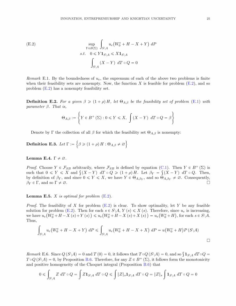
INNOVATION, ENTREPRENEURSHIP AND KNIGHTIAN UNCERTAINTY 25
supY PBpΣq
ż
SzAue
`W e
0 `H ´X ` Y˘dP(E.2)
s.t. 0 ď Y 1SzA ď X1SzAż
SzApX ´ Y q dT ˝Q “ 0
Remark E.1. By the boundedness of ue, the supremum of each of the above two problems is finitewhen their feasibility sets are nonempty. Now, the function X is feasible for problem (E.2), and soproblem (E.2) has a nonempty feasibility set.
Definition E.2. For a given β ě p1 ` ρqH, let ΘA,β be the feasibility set of problem (E.1) withparameter β. That is,
ΘA,β :“
#Y P B` pΣq : 0 ď Y ď X,
żpX ´ Y q dT ˝ Q “ β
+
Denote by Γ the collection of all β for which the feasibility set ΘA,β is nonempty:
Definition E.3. Let Γ :“!β ě p1 ` ρqH : ΘA,β ‰ ∅
)
Lemma E.4. Γ ‰ ∅.
Proof. Choose Y P FSB arbitrarily, where FSB is defined by equation (C.1). Then Y P B` pΣq issuch that 0 ď Y ď X and
şpX ´ Y q dT ˝ Q ě p1 ` ρqH. Let βY “
şpX ´ Y q dT ˝ Q. Then,
by definition of βY , and since 0 ď Y ď X, we have Y P ΘA,βY, and so ΘA,βY
‰ ∅. Consequently,βY P Γ, and so Γ ‰ ∅. �
Lemma E.5. X is optimal for problem (E.2).
Proof. The feasibility of X for problem (E.2) is clear. To show optimality, let Y be any feasiblesolution for problem (E.2). Then for each s P SzA, Y psq ď X psq. Therefore, since ue is increasing,we have ue
`W e
0 `H´X psq`Y psq˘
ď ue`W e
0 `H´X psq`X psq˘
“ ue`W e
0 `H˘, for each s P SzA.
Thus,ż
SzAue
`W e
0 `H ´X ` Y˘dP ď
ż
SzAue
`W e
0 `H ´X `X˘dP “ u
`W e
0 `H˘P pSzAq
�
Remark E.6. Since Q pSzAq “ 0 and T p0q “ 0, it follows that T ˝Q pSzAq “ 0, and soş1SzA dT ˝Q “
T ˝Q pSzAq “ 0, by Proposition B.6. Therefore, for any Z P B` pΣq, it follows form the monotonicityand positive homogeneity of the Choquet integral (Proposition B.6) that
0 ď
ż
SzAZ dT ˝ Q “
żZ1SzA dT ˝ Q ď
ż}Z}s1SzA dT ˝Q “ }Z}s
ż1SzA dT ˝ Q “ 0

26 MASSIMILIANO AMARANTE, MARIO GHOSSOUB, AND EDMUND PHELPS
and soşSzAZ dT ˝ Q “ 0. Consequently, it follows form Proposition B.6 that for any Z P B` pΣq,
żZ dT ˝ Q ď
żZ1A dT ˝ Q “
ż
A
Z dT ˝ Q
Now, consider the following problem:
supβPΓ
#F ˚A pβq : F ˚
A pβq is the supremum of problem (E.1), for a fixed β P Γ
+(E.3)
Lemma E.7. Under Assumption 7.1, if β˚ is optimal for problem (E.3), and if Y ˚1 is optimal for
problem (E.1) with parameter β˚, then Y ˚ :“ Y ˚1 1A ` X1SzA is optimal for problem (4.1) (with
υ “ T ˝ Q).
Proof. By the feasibility of Y ˚1 for problem (E.1) with parameter β˚, we have 0 ď Y ˚
1 ď X andşpX ´ Y ˚
1 q dT ˝ P “ β˚. Therefore, 0 ď Y ˚ ď X, andż
pX ´ Y ˚q dT ˝ Q “
ż “pX ´ Y ˚
1 q1A ` pX ´Xq1SzA
‰dT ˝ Q
“
ż
A
pX ´ Y ˚1 q dT ˝Q ě
żpX ´ Y ˚
1 q dT ˝Q “ β˚ ě p1 ` ρqH
where the inequalityşA
pX ´ Y ˚1 q dT ˝ Q ě
şpX ´ Y ˚
1 q dT ˝ Q follows from the same argument asin Remark E.6. Hence, Y ˚ is feasible for problem (4.1) (with υ “ T ˝ Q). To show optimality ofY ˚ for problem (4.1) (with υ “ T ˝ Q), let Y be any other feasible function for problem (4.1) (withυ “ T ˝ Q), and define α by α “
ş `X ´ Y
˘dT ˝ Q. Then α ě p1 ` ρqH, and so Y is feasible for
problem (E.1) with parameter α, and α is feasible for problem (E.3). Hence
F ˚A pαq ě
ż
A
ue`W e
0 `H ´X ` Y˘dP
Now, since β˚ is optimal for problem (E.3), it follows that F ˚A pβ˚q ě F ˚
A pαq. Moreover, Y is
feasible for problem (E.2) (since 0 ď Y ď X and soşSzA
`X ´ Y
˘dT ˝Q “ 0 by Remark E.6). Thus,
F ˚A pβ˚q ` ue
`W e
0 `H˘P pSzAq ě F ˚
A pαq ` ue`W e
0 `H˘P pSzAq
ě
ż
A
ue`W e
0 `H ´X ` Y˘dP ` ue
`W e
0 `H˘P pSzAq
ě
ż
A
ue`W e
0 `H ´X ` Y˘dP `
ż
SzAue
`W e
0 `H ´X ` Y˘dP
“
żue
`W e
0 `H ´X ` Y˘dP
However, F ˚A pβ˚q “
şAue
`W e
0 `H ´X ` Y ˚1
˘dP . Therefore,
żue
`W e
0 `H ´X ` Y ˚˘dP “ F ˚
A pβ˚q ` ue`W e
0 `H˘P pSzAq ě
żue
`W e
0 `H ´X ` Y˘dP
Hence, Y ˚ is optimal for problem (4.1) (with υ “ T ˝Q). �
Remark E.8. By Lemma E.7, we can restrict ourselves to solving problem (E.1) with a parameterβ P Γ.

INNOVATION, ENTREPRENEURSHIP AND KNIGHTIAN UNCERTAINTY 27
E.2. Solving Problem (E.1). Recall that for all Z P B pΣq,şZ dP “
şAZh dQ`
şSzA Z dP , where
h “ dPac{dQ is the Radon-Nikodym derivative of Pac with respect to Q. Moreover, by definition ofthe set A P Σ, we have Q pSzAq “ Ps pAq “ 0. Therefore,
şAZh dQ “
şZh dQ, for each Z P B pΣq.
Hence, we can rewrite problem (E.1) (restricting ourselves to parameters β P Γ and recalling thath “ φ ˝ X) as the following problem:
For a given β P Γ,
supY PBpΣq
żue
`W e
0 `H ´X ` Y˘φ pXq dQ(E.4)
s.t. 0 ď Y ď Xż
pX ´ Y q dT ˝Q “ β
Now, consider the following problem:
For a given β P Γ,
supY PBpΣq
żue
`W e
0 `H ´ Z˘φ pXq dQ(E.5)
s.t. 0 ď Z ď XżZ dT ˝ Q “ β “
ż `8
0
T´Q
`ts P S : Z psq ě tu
˘¯dt
Lemma E.9. If Z˚ is optimal for problem (E.5) with parameter β, then Y ˚ :“ X ´ Z˚ is optimalfor problem (E.4) with parameter β.
Proof. Let β P Γ be given, and suppose that Z˚ is optimal for problem (E.5) with parameter β.Define Y ˚ :“ X ´ Z˚. Then Y ˚ P B pΣq. Moreover, since 0 ď Z˚ ď X, it follows that 0 ď Y ˚ ď X.Now, ż
pX ´ Y ˚q dT ˝ Q “
ż ´X ´ pX ´ Z˚q
¯dT ˝ Q “
żZ˚ dT ˝ Q “ β
and so Y ˚ is feasible for problem (E.4) with parameter β. To show optimality of Y ˚ for problem(E.4) with parameter β, suppose, by way of contradiction, that Y ‰ Y ˚ is feasible for problem (E.4)with parameter β and
żue
`W e
0 `H ´X ` Y˘h dQ ą
żue
`W e
0 `H ´X ` Y ˚˘h dQ
that is, with Z :“ X ´ Y , we haveżue
`W e
0 `H ´ Z˘h dQ ą
żue
`W e
0 `H ´ Z˚˘h dQ
Now, since 0 ď Y ď X andş `X ´ Y
˘dT ˝Q “ β, we have that Z is feasible for problem (E.5) with
parameter β, hence contradicting the optimality of Z˚ for problem (E.5) with parameter β. Thus,Y ˚ :“ X ´ Z˚ is optimal for problem (E.4) with parameter β. �
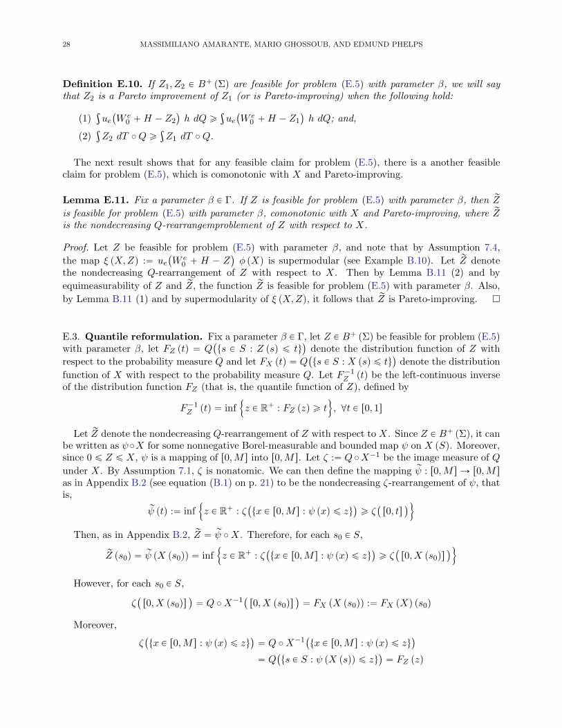
28 MASSIMILIANO AMARANTE, MARIO GHOSSOUB, AND EDMUND PHELPS
Definition E.10. If Z1, Z2 P B` pΣq are feasible for problem (E.5) with parameter β, we will saythat Z2 is a Pareto improvement of Z1 (or is Pareto-improving) when the following hold:
(1)şue
`W e
0 `H ´ Z2
˘h dQ ě
şue
`W e
0 `H ´ Z1
˘h dQ; and,
(2)şZ2 dT ˝ Q ě
şZ1 dT ˝ Q.
The next result shows that for any feasible claim for problem (E.5), there is a another feasibleclaim for problem (E.5), which is comonotonic with X and Pareto-improving.
Lemma E.11. Fix a parameter β P Γ. If Z is feasible for problem (E.5) with parameter β, then rZis feasible for problem (E.5) with parameter β, comonotonic with X and Pareto-improving, where rZis the nondecreasing Q-rearrangemproblement of Z with respect to X.
Proof. Let Z be feasible for problem (E.5) with parameter β, and note that by Assumption 7.4,
the map ξ pX,Zq :“ ue`W e
0 ` H ´ Z˘φ pXq is supermodular (see Example B.10). Let rZ denote
the nondecreasing Q-rearrangement of Z with respect to X. Then by Lemma B.11 (2) and by
equimeasurability of Z and rZ, the function rZ is feasible for problem (E.5) with parameter β. Also,
by Lemma B.11 (1) and by supermodularity of ξ pX,Zq, it follows that rZ is Pareto-improving. �
E.3. Quantile reformulation. Fix a parameter β P Γ, let Z P B` pΣq be feasible for problem (E.5)with parameter β, let FZ ptq “ Q
`ts P S : Z psq ď tu
˘denote the distribution function of Z with
respect to the probability measure Q and let FX ptq “ Q`ts P S : X psq ď tu
˘denote the distribution
function of X with respect to the probability measure Q. Let F´1Z ptq be the left-continuous inverse
of the distribution function FZ (that is, the quantile function of Z), defined by
F´1Z ptq “ inf
!z P R
` : FZ pzq ě t), @t P r0, 1s
Let rZ denote the nondecreasing Q-rearrangement of Z with respect to X. Since Z P B` pΣq, it canbe written as ψ˝X for some nonnegative Borel-measurable and bounded map ψ on X pSq. Moreover,since 0 ď Z ď X, ψ is a mapping of r0,M s into r0,M s. Let ζ :“ Q ˝X´1 be the image measure of Q
under X. By Assumption 7.1, ζ is nonatomic. We can then define the mapping rψ : r0,M s Ñ r0,M sas in Appendix B.2 (see equation (B.1) on p. 21) to be the nondecreasing ζ-rearrangement of ψ, thatis,
rψ ptq :“ inf!z P R
` : ζ`tx P r0,M s : ψ pxq ď zu
˘ě ζ
`r0, ts
˘)
Then, as in Appendix B.2, rZ “ rψ ˝X. Therefore, for each s0 P S,
rZ ps0q “ rψ pX ps0qq “ inf!z P R
` : ζ`tx P r0,M s : ψ pxq ď zu
˘ě ζ
`r0,X ps0qs
˘)
However, for each s0 P S,
ζ`
r0,X ps0qs˘
“ Q ˝X´1`
r0,X ps0qs˘
“ FX pX ps0qq :“ FX pXq ps0q
Moreover,
ζ`tx P r0,M s : ψ pxq ď zu
˘“ Q ˝X´1
`tx P r0,M s : ψ pxq ď zu
˘
“ Q`ts P S : ψ pX psqq ď zu
˘“ FZ pzq
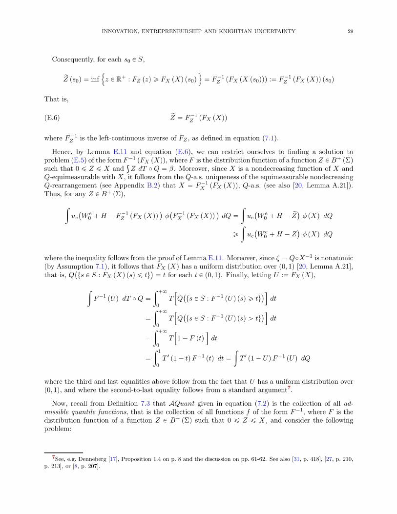
INNOVATION, ENTREPRENEURSHIP AND KNIGHTIAN UNCERTAINTY 29
Consequently, for each s0 P S,
rZ ps0q “ inf!z P R
` : FZ pzq ě FX pXq ps0q)
“ F´1Z pFX pX ps0qqq :“ F´1
Z pFX pXqq ps0q
That is,
(E.6) rZ “ F´1Z pFX pXqq
where F´1Z is the left-continuous inverse of FZ , as defined in equation (7.1).
Hence, by Lemma E.11 and equation (E.6), we can restrict ourselves to finding a solution toproblem (E.5) of the form F´1 pFX pXqq, where F is the distribution function of a function Z P B` pΣqsuch that 0 ď Z ď X and
şZ dT ˝ Q “ β. Moreover, since X is a nondecreasing function of X and
Q-equimeasurable with X, it follows from the Q-a.s. uniqueness of the equimeasurable nondecreasingQ-rearrangement (see Appendix B.2) that X “ F´1
X pFX pXqq, Q-a.s. (see also [20, Lemma A.21]).Thus, for any Z P B` pΣq,
żue
`W e
0 `H ´ F´1Z pFX pXqq
˘φ
`F´1X pFX pXqq
˘dQ “
żue
`W e
0 `H ´ rZ˘φ pXq dQ
ě
żue
`W e
0 `H ´ Z˘φ pXq dQ
where the inequality follows from the proof of Lemma E.11. Moreover, since ζ “ Q˝X´1 is nonatomic(by Assumption 7.1), it follows that FX pXq has a uniform distribution over p0, 1q [20, Lemma A.21],that is, Q
`ts P S : FX pXq psq ď tu
˘“ t for each t P p0, 1q. Finally, letting U :“ FX pXq,
żF´1 pUq dT ˝Q “
ż `8
0
T”Q
`ts P S : F´1 pUq psq ě tu
˘ıdt
“
ż `8
0
T”Q
`ts P S : F´1 pUq psq ą tu
˘ıdt
“
ż `8
0
T”1 ´ F ptq
ıdt
“
ż 1
0
T 1 p1 ´ tqF´1 ptq dt “
żT 1 p1 ´ UqF´1 pUq dQ
where the third and last equalities above follow from the fact that U has a uniform distribution overp0, 1q, and where the second-to-last equality follows from a standard argument7.
Now, recall from Definition 7.3 that AQuant given in equation (7.2) is the collection of all ad-missible quantile functions, that is the collection of all functions f of the form F´1, where F is thedistribution function of a function Z P B` pΣq such that 0 ď Z ď X, and consider the followingproblem:
7See, e.g. Denneberg [17], Proposition 1.4 on p. 8 and the discussion on pp. 61-62. See also [31, p. 418], [27, p. 210,p. 213], or [8, p. 207].

30 MASSIMILIANO AMARANTE, MARIO GHOSSOUB, AND EDMUND PHELPS
For a given β P Γ
supf
V pfq “
żue
`W e
0 `H ´ f pUq˘φ
`F´1X pUq
˘dQ(E.7)
s.t. f P AQuantżT 1 p1 ´ Uq f pUq dQ “ β
Lemma E.12. If f˚ is optimal for problem (E.7) with parameter β P Γ, then the function f˚ pUq isoptimal for problem (E.5) with parameter β, where U :“ FX pXq. Moreover, X ´ f˚ pUq is optimalfor problem (E.4) with parameter β.
Proof. Fix β P Γ, suppose that f˚ P AQuant is optimal for problem (E.7) with parameter β and letZ˚ P B` pΣq be a corresponding function. That is, f˚ is the quantile function of Z˚ and 0 ď Z˚ ď X.
Let rZ˚ :“ f˚ pUq. Then rZ˚ is the equimeasurable nondecreasing Q-rearrangement of Z˚ with respect
to X, and so 0 ď rZ˚ ď X by Lemma B.11 (2). Moreover,
β “
żT 1 p1 ´ Uq f˚ pUq dQ “
żf˚ pUq dT ˝ Q
“
żrZ˚ dT ˝ Q “
ż `8
0
T”Q
`ts P S : rZ˚ psq ě tu
˘ıdt
“
ż `8
0
T”Q
`ts P S : Z˚ psq ě tu
˘ıdt “
żrZ˚ dT ˝Q
where the second-to-last equality follows from the Q-equimeasurability of Z˚ and rZ˚. Therefore,rZ˚ “ f˚ pUq is feasible for problem (E.5) with parameter β. To show optimality, let Z be anyfeasible solution for problem (E.5) with parameter β and let F be the distribution function for Z.
Then, by Lemma E.11, the function rZ :“ F´1 pUq is feasible for problem (E.5) with parameter β,
comonotonic with X and Pareto-improving. Moreover, rZ has also F as a distribution function. To
show optimality of rZ˚ “ f˚ pUq for problem (E.5) with parameter β it remains to show thatżue
`W e
0 `H ´ rZ˚˘φ pXq dQ ě
żue
`W e
0 `H ´ rZ˘φ pXq dQ
Now, let f :“ F´1, so that rZ “ f pUq. Since rZ is feasible for problem (E.5) with parameter β, wehave
β “
żrZ dT ˝ Q “
żF´1 pUq dT ˝ Q
“
ż 1
0
T 1 p1 ´ tqF´1 ptq dt “
żT 1 p1 ´ Uq f pUq dQ
Hence, f is feasible for problem (E.7) with parameter β. Since f˚ is optimal for problem (E.7) withparameter β we have
żue
`W e
0 `H ´ f˚ pUq˘φ
`F´1X pUq
˘dQ ě
żue
`W e
0 `H ´ f pUq˘φ
`F´1X pUq
˘dQ

INNOVATION, ENTREPRENEURSHIP AND KNIGHTIAN UNCERTAINTY 31
Finally, since X “ F´1X pUq , Q-a.s., we have
żue
`W e
0 `H ´ rZ˚˘φ pXq dQ ě
żue
`W e
0 `H ´ rZ˘φ pXq dQ
Therefore, rZ˚ “ f˚ pUq is optimal for problem (E.5) with parameter β. Finally, by Lemma E.9,
Y ˚ :“ X ´ rZ˚ “ X ´ f˚ pUq is optimal for problem (E.4) with parameter β. �
By Lemmata E.7 and E.12, this completes the proof of Theorem 7.5. l
Appendix F. Proof of Corollary 7.8
Corollary F.1. Under the assumptions of Section 7, there exists a parameter β˚ ě p1 ` ρqH suchthat an optimal solution Y ˚ for problem (4.1) (with υ “ T ˝ Q) takes the following form:
Y ˚ “
˜X ´ max
«0,min
!F´1X pUq , f˚
λ˚ pUq)ff¸
1A `X1SzA
where for each t P p0, 1q ztt : φ ˝ F´1x ptq “ 0u,
f˚λ˚ ptq “ W e
0 `H ´`u1e
˘´1
˜´λ˚T 1 p1 ´ tq
φ`F´1X ptq
˘¸
and λ˚ is chosen so thatż 1
0
T 1 p1 ´ tqmax”0,min
!F´1X ptq , f˚
λ˚ ptq)ı
dt “ β˚
Proof. Recall from equation (7.2) that
AQuant “!f P Quant : 0 ď f pzq ď F´1
X pzq , for each 0 ă z ă 1),
where Quant “!f : p0, 1q Ñ R
ˇˇ f is nondecreasing and left-continuous
). Define the collection K of
functions on p0, 1q as follows:
(F.1) K “!f : p0, 1q Ñ R
ˇˇ 0 ď f pzq ď F´1
X pzq , for each 0 ă z ă 1)
Then AQuant “ QuantX K. Consider the following problem, with parameter β P Γ:
For a given β P Γ
supf
V pfq “
ż 1
0
ue`W e
0 `H ´ f ptq˘φ
`F´1X ptq
˘dt(F.2)
s.t. f P AQuantż 1
0
T 1 p1 ´ tq f ptq dt “ β
Lemma F.2. For a given β P Γ, if f˚ P AQuant satisfies the following:
(1)ş10T 1 p1 ´ tq f˚ ptq dt “ β;
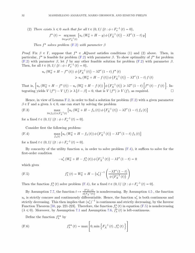
32 MASSIMILIANO AMARANTE, MARIO GHOSSOUB, AND EDMUND PHELPS
(2) There exists λ ď 0 such that for all t P p0, 1q ztt : φ ˝ F´1x ptq “ 0u,
f˚ ptq “ argmax0ďyďF´1
Xptq
“ue pW e
0 `H ´ yqφ`F´1X ptq
˘´ λT 1 p1 ´ tq y
‰
Then f˚ solves problem (F.2) with parameter β
Proof. Fix β P Γ, suppose that f˚ P AQuant satisfies conditions p1q and p2q above. Then, inparticular, f˚ is feasible for problem (F.2) with parameter β. To show optimality of f˚ for problem(F.2) with parameter β, let f by any other feasible solution for problem (F.2) with parameter β.Then, for all t P p0, 1q ztt : φ ˝ F´1
x ptq “ 0u,
ue pW e0 `H ´ f˚ ptqq φ
`F´1X ptq
˘´ λT 1 p1 ´ tq f˚ ptq
ě ue pW e0 `H ´ f ptqqφ
`F´1X ptq
˘´ λT 1 p1 ´ tq f ptq
That is,”ue pW e
0 `H ´ f˚ ptqq ´ ue pW e0 `H ´ f ptqq
ıφ
`F´1X ptq
˘ě λT 1 p1 ´ tq
”f˚ ptq ´ f ptq
ı. In-
tegrating yields V pf˚q ´ V pfq ě λ rβ ´ βs “ 0, that is V pf˚q ě V pfq, as required. �
Hence, in view of Lemma F.2, in order to find a solution for problem (F.2) with a given parameterβ P Γ and a given λ ď 0, one can start by solving the problem
(F.3) max0ďfλptqďF´1
Xptq
“ue pW e
0 `H ´ fλ ptqqφ`F´1X ptq
˘´ λT 1 p1 ´ tq fλ ptq
‰
for a fixed t P p0, 1q ztt : φ ˝ F´1x ptq “ 0u.
Consider first the following problem:
(F.4) maxfλptq
“ue pW e
0 `H ´ fλ ptqqφ`F´1X ptq
˘´ λT 1 p1 ´ tq fλ ptq
‰
for a fixed t P p0, 1q ztt : φ ˝ F´1x ptq “ 0u.
By concavity of the utility function u, in order to solve problem (F.4), it suffices to solve for thefirst-order condition
´u1e pW e
0 `H ´ f˚λ ptqqφ
`F´1X ptq
˘´ λT 1 p1 ´ tq “ 0
which gives
(F.5) f˚λ ptq “ W e
0 `H ´`u1e
˘´1
˜´λT 1 p1 ´ tq
φ`F´1X ptq
˘¸
Then the function f˚λ ptq solve problem (F.4), for a fixed t P p0, 1q ztt : φ ˝ F´1
x ptq “ 0u.
By Assumption 7.7, the function t ÞÑ T 1p1´tq
φpF´1
Xptqq
is nondecreasing. By Assumption 4.5 , the function
ue is strictly concave and continuously differentiable. Hence, the function u1e is both continuous and
strictly decreasing. This then implies that pu1eq´1 is continuous and strictly decreasing, by the Inverse
Function Theorem [50, pp. 221-223]. Therefore, the function f˚λ ptq in equation (F.5) is nondecreasing
(λ ď 0). Moreover, by Assumption 7.1 and Assumption 7.6, f˚λ ptq is left-continuous.
Define the function f˚˚λ by
(F.6) f˚˚λ ptq “ max
«0,min
!F´1X ptq , f˚
λ ptq)ff

INNOVATION, ENTREPRENEURSHIP AND KNIGHTIAN UNCERTAINTY 33
Then f˚˚λ ptq P K. Moreover, since both F´1
X and f˚λ are nondecreasing and left-continuous functions,
it follows that f˚˚λ is nondecreasing and left-continuous. Consequently, f˚˚
λ ptq P AQuant. Finally,it is easily seen that f˚˚
λ ptq solves problem (F.3) for the given λ. Now, for a given β0 P Γ, if λ˚ is
chosen so thatş10T 1 p1 ´ tq f˚˚
λ˚ ptq dt “ β0, then by Lemma F.2, f˚˚λ˚ is optimal for problem (F.2)
with parameter β0.
Hence, in view of Theorem 7.5, to conclude the proof of Corollary 7.8, it remains to show that for
each β0 P Γ, there exists a λ˚ ď 0 such thatş10T 1 p1 ´ tq f˚˚
λ˚ ptq dt “ β0. This is given by LemmaF.3 below.
Lemma F.3. Let ψ be the function of the parameter λ ď 0 defined by ψ pλq :“ş10T 1 p1 ´ tq f˚˚
λ ptq dt.Then for each β0 P Γ, there exists a λ˚ ď 0 such that ψ pλ˚q “ β0.
Proof. First note that ψ is a continuous and nonincreasing function of λ, where continuity of ψ is aconsequence of Lebesgue’s Dominated Convergence Theorem [1, Theorem 11.21]. Indeed, since X isbounded and since F´1
X is nondecreasing, it follows that for each t P r0, 1s,
min!F´1X ptq , f˚
λ ptq)
ď F´1X ptq ď F´1
X p1q ď M “ }X}s ă `8.
Moreover, since T is concave and increasing, T 1 is nonincreasing and nonnegative, and so for eacht P r0, 1s, 0 ď T 1 p1 ´ tq ď T 1 p0q. But T 1 p0q ă `8, by Assumption 7.1. Hence, for each t P r0, 1s,
min!F´1X ptq , f˚
λ ptq)T 1 p1 ´ tq ď F´1
X p1qT 1 p0q ď }X}s T1 p0q ă `8
Moreover, ψ p0q “ 0 (by Assumption 4.5), and
limλÑ´8
ψ pλq “
ż 1
0
T 1 p1 ´ tqmin!F´1X ptq ,W e
0 `H)dt
“
ż FXpW e0
`Hq
0
T 1 p1 ´ tqF´1X ptq dt ` pW e
0 `Hq
ż 1
FXpW e0
`HqT 1 p1 ´ tq dt
However, by Assumption 7.2, we have FX pW e0 `Hq “ 1. This then implies that
limλÑ´8
ψ pλq “
ż 1
0
T 1 p1 ´ tqF´1X ptq dt “
żX dT ˝ Q
Now, for any β0 P Γ, and for any Y P B` pΣq which is feasible for problem (E.1) with parameterβ0, one has:
(i) 0 ď Y ď X; and,
(ii)ş
pX ´ Y q dT ˝Q “ β0.
Hence, 0 ď X´Y ď X, and so, by monotonicity of the Choquet integral (Proposition B.6), it followsthat β0 “
şpX ´ Y q dT ˝ Q ď
şX dT ˝Q. Consequently, for any β0 P Γ,
0 “ ψ p0q ď β0 ď
żX dT ˝ Q “ lim
λÑ´8ψ pλq
Hence, by the Intermediate Value Theorem [50, Theorem 4.23], for each β0 P Γ there exists someλ˚ ď 0 such that ψ pλ˚q “ β0. �
By Lemmata F.2 and F.3, this concludes the proof of Corollary F.1. �

34 MASSIMILIANO AMARANTE, MARIO GHOSSOUB, AND EDMUND PHELPS
Now, since the function f˚˚λ ptq “ max
«0,min
!F´1X ptq , f˚
λ˚ ptq)ff
is optimal for problem (F.2)
with parameter β˚, it is optimal for problem (E.7) with parameter β˚. Therefore, by Lemma E.12,the function
f˚˚λ pUq “ max
«0,min
!F´1X pUq , f˚
λ˚ pUq)ff
is optimal for problem (E.5) with parameter β˚. However, since Q˝X´1 is nonatomic (by Assumption7.1), it follows that FX pXq has a uniform distribution over p0, 1q [20, Lemma A.21], and that X “F´1X pFX pXqq , Q-a.s. Therefore,
f˚˚λ pUq “ max
«0,min
!F´1X pUq , f˚
λ˚ pUq)ff
“ max
«0,min
!F´1X pUq ,W e
0 `H ´`u1e
˘´1
˜´λ˚T 1 p1 ´ Uq
φ`F´1X pUq
˘¸ )ff
“ max
«0,min
#X,W e
0 `H ´`u1e
˘´1
ˆ´λ˚T 1 p1 ´ Uq
φ pXq
˙ +ff, Q-a.s.
This Q-a.s. equality implies that
max
«0,min
#X,W e
0 `H ´`u1e
˘´1
ˆ´λ˚T 1 p1 ´ Uq
φ pXq
˙ +ff
is also optimal for problem (E.5) with parameter β˚. Lemma E.9 then implies that
X ´ max
«0,min
#X,W e
0 `H ´`u1e
˘´1
ˆ´λ˚T 1 p1 ´ Uq
φ pXq
˙ +ff
is optimal for problem (E.4) (and hence for problem (E.1)) with parameter β˚. Finally, it can easilybe verified that
X´max
«0,min
#X,W e
0 `H ´`u1e
˘´1
ˆ´λ˚T 1 p1 ´ Uq
φ pXq
˙ +ff
“ min
«X,max
˜0,X ´
„W e
0 `H ´`u1e
˘´1
ˆ´λ˚T 1 p1 ´ Uq
φ pXq
˙ ¸ff
The rest follows form Lemma E.7 and Corollary F.1, noting that since X “ F´1X pUq , Q-a.s., one
has:
β˚ “
ż 1
0
T 1 p1 ´ tqmax”0,min
!F´1X ptq , f˚
λ˚ ptq)ı
dt
“
żT 1 p1 ´ Uqmax
”0,min
!F´1X pUq , f˚
λ˚ pUq)ı
dQ
“
żT 1 p1 ´ Uqmax
«0,min
#X,W e
0 `H ´`u1e
˘´1
ˆ´λ˚T 1 p1 ´ Uq
φ pXq
˙ +ffdQ
This concludes the proof of Corollary 7.8. l

INNOVATION, ENTREPRENEURSHIP AND KNIGHTIAN UNCERTAINTY 35
References
[1] C.D. Aliprantis and K.C. Border. Infinite Dimensional Analysis - 3rd edition. Springer-Verlag, 2006.
[2] M. Amarante, O. Ozgur, and E.S. Phelps. The Entrepreneurial Economy II: Equilibria and Welfare. mimeo(2011).
[3] M. Amarante and E.S. Phelps. The Entrepreneurial Economy. Kauffman Foundation Report, 2005.[4] W.J. Baumol. Entrepreneurship in Economic Theory. The American Economic Review, 58(2):64–71, 1968.[5] M. Bianchi and M. Henrekson. Is Neoclassical Economics Still Entrepreneurless? Kyklos, 58(3):353–377, 2005.[6] R. Bojilov and E.S. Phelps. Dynamism and Economic Performance: A Preliminary Report. Columbia University,
The Center on Capitalism and Society, Working Paper No. 60 (July 2010).[7] M. Boldrin and D.K. Levine. Perfectly Competitive Innovation. Journal of Monetary Economics, 55(3):435–453,
2008.[8] G. Carlier and R.A. Dana. Core of Convex Distortions of a Probability. Journal of Economic Theory, 113(2):199–
222, 2003.[9] G. Carlier and R.A. Dana. Pareto Efficient Insurance Contracts when the Insurer’s Cost Function is Discontin-
uous. Economic Theory, 21(4):871–893, 2003.[10] G. Carlier and R.A.Dana. Rearrangement Inequalities in Non-convex Insurance Models. Journal of Mathematical
Economics, 41(4-5):483–503, 2005.[11] G. Carlier and R.A.Dana. Two-persons Efficient Risk-sharing and Equilibria for Concave Law-invariant Utilities.
Economic Theory, 36(2):189–223, 2008.[12] G. Carlier and R.A. Dana. Optimal Demand for Contingent Claims when Agents Have Law Invariant Utilities.
Mathematical Finance, 21(2):169–201, 2011.[13] N.L. Carothers. Real Analysis. Cambridge University Press, 2000.[14] A. Chateauneuf, R.A. Dana, and J.M. Tallon. Optimal Risk-sharing Rules and Equilibria with Choquet-
expected-utility. Journal of Mathematical Economics, 34(2):191–214, 2000.[15] D.L. Cohn. Measure Theory. Birkhauser, 1980.[16] R.A. Dana. On Equilibria when Agents have Multiple Priors. Annals of Operations Research, 114(1):105–115,
2002.[17] D. Denneberg. Non-Additive Measure and Integral. Kluwer Academic Publishers, 1994.[18] R.M. Dudley. Real Analysis and Probability. Cambridge University Press, 2002.[19] A.M. Endres and C.R. Woods. Modern Theories of Entrepreneurial Behavior: A Comparison and Appraisal.
Small Business Economics, 26(2):189–202, 2006.[20] H. Follmer and A. Schied. Stochastic Finance: An Introduction in Discrete Time – 3rd ed. Walter de Gruyter,
2011.[21] P.Ghirardato, F.Maccheroni, and M. Marinacci. Differentiating Ambiguity and Ambiguity Attitude. Journal
of Economic Theory, 118(2):133–173, 2004.[22] P. Ghirardato and M. Siniscalchi. A More Robust Definition of Multiple Priors. mimeo (2010).[23] M. Ghossoub. Belief Heterogeneity in the Arrow-Borch-Raviv Insurance Model. mimeo (2011).[24] M. Ghossoub. Monotone Equimeasurable Rarrangements with Non-Additive Probabilities. mimeo (2011).[25] I. Gilboa and M. Marinacci. Ambiguity and the Bayesian Paradigm. In D. Acemoglu, M. Arellano, and E.
Dekel (eds.), Advances in Economics and Econometrics: Theory and Applications, Tenth World Congress of theEconometric Society. Cambridge University Press, 2012.
[26] I. Gilboa and D. Schmeidler. Maxmin Expected Utility with a Non-Unique Prior. Journal of MathematicalEconomics, 18(2):141–153, 1989.
[27] X.D. He and X.Y. Zhou. Portfolio Choice via Quantiles. Mathematical Finance, 21(2):203–231, 2011.[28] H.T. Hoon and E.S. Phelps. Innovation and Employment. Columbia University, The Center on Capitalism and
Society, Working Paper No. 69 (April 2011).[29] P.J. Huber and E.M. Ronchetti. Robust Statistics - Second Edition. John Wiley and Sons, 2011.[30] H. Jin and X.Y. Zhou. Greed, Leverage, and Potential Losses: A Prospect Theory Perspective. Mathematical
Finance, Forthcoming.[31] H. Jin and X.Y. Zhou. Behavioral Portfolio Selection in Continous Time. Mathematical Finance, 18(3):385–426,
2008.[32] J.B. Kadane and L. Wasserman. Symmetric, Coherent, Choquet Capacities. The Annals of Statistics, 24(3):1250–
1264, 1996.[33] D. Kahneman and A. Tversky. Prospect Theory: An Analysis of Decision Under Risk. Econometrica, 47(2):263–
291, 1979.[34] R.E. Kihlstrom and J.J. Laffont. A General Equilibrium Entrepreneurial Theory of Firm Formation Based on
Risk Aversion. Journal of Political Economy, 87(4):719–748, 1979.

36 MASSIMILIANO AMARANTE, MARIO GHOSSOUB, AND EDMUND PHELPS
[35] I.M. Kirzner. Entrepreneurial Discovery and the Competitive Market Process: An Austrian Approach. Journalof Economic Literature, 35(1):60–85, 1997.
[36] F.H. Knight. Risk, Uncertainty, and Profit. Boston/New York: Houghton Mifflin, 1921.[37] R.E. Lucas. On the Size Distribution of Business Firms. The Bell Journal of Economics, 9(2):508–523, 1978.[38] M. Marinacci and L. Montrucchio. Introduction to the Mathematics of Ambiguity. In I. Gilboa (ed.), Uncer-
tainty in Economic Theory: Essays in Honor of David Schmeidlers 65th Birthday. Routledge, London, 2004.[39] P. Milgrom. Good News and Bad News: Representation Theorems and Applications. The Bell Journal of Eco-
nomics, 12(2):380–391, 1981.[40] S. Mukerji. Ambiguity Aversion and Incompleteness of Contractual Form. American Economic Review,
88(5):1207–1231, 1998.[41] S. Mukerji. A Survey of Some Applications of the Idea of Ambiguity Aversion in Economics. International Journal
of Approximate Reasoning, 24(2):221–234, 2000.[42] S. Mukerji and J.M. Tallon. An Overview of Economic Applications of David Schmeidlers Models of Deci-
sion Making under Uncertainty. In I. Gilboa (ed.), Uncertainty in Economic Theory: Essays in Honor of DavidSchmeidlers 65th Birthday. Routledge, London, 2004.
[43] E. Pap. Null-Additive Set Functions. Kluwer Academic Publishers, 1995.[44] E.S. Phelps. The Economic Prosperity of Nations: Prosperity Depends on Dynamism, Dynamism on Institutions.
Columbia University, The Center on Capitalism and Society, Working Paper No. 2 (January 2005).[45] E.S. Phelps. Toward a Model of Innovation and Performance Along the Lines of Knight, Keynes, Hayek and m.
Polanyı. Columbia University, The Center on Capitalism and Society, Working Paper No. 19 (November 2006).[46] R. Pollock. Economics Bibliography: Primarily Innovation and IP Oriented.
http://rufuspollock.org/economics/biblio/.[47] J. Quiggin. A Theory of Anticipated Utility. Journal of Economic Behavior, 3(4):323–343, 1982.[48] J. Reinganum. The Timing of Innovation: Research, Development, and Diffusion. In R. Schmalensee & R. Willig
(ed.), Handbook of Industrial Organization, vol. 1, ch. 14, 849-908. Elsevier, 1989.[49] P.M. Romer. Increasing Returns and Long-Run Growth. The Journal of Political Economy, 94(5):1002–1037,
1986.[50] W. Rudin. Principles of Mathematical Analysis – 3rd ed. New York: McGraw-Hill Book Company, 1976.[51] D. Schmeidler. Integral Representation without Additivity. Proceedings of the American Mathematical Society,
97(2):255–261, 1986.[52] D. Schmeidler. Subjective Probability and Expected Utility without Additivity. Econometrica, 57(3):571–587,
1989.[53] J.A. Schumpeter. The Theory of Economic Development. Cambridge: Harvard University Press [English Trans-
lation 1936], 1911.[54] S. Scotchmer. Innovation and Incentives. The MIT Press, 2004.[55] A. Tversky and D. Kahneman. Advances in Prospect Theory: Cumulative Representation of Uncertainty. The
Journal of Risk and Uncertainty, 5(4):297–323, 1992.[56] L. Wasserman and J.B. Kadane. Symmetric Upper Probabilities. The Annals of Statistics, 20(4):1720–1736,
1992.[57] M. Yaari. The Dual Theory of Choice under Risk. Econometrica, 55(1):95–115, 1987.
Massimiliano Amarante: Universite de Montreal – Departement de Sciences Economiques – C.P.
6128, succursale Centre-ville – Montreal, QC, H3C 3J7 – Canada
E-mail address: [email protected]
Mario Ghossoub: Imperial College Business School – Imperial College London – South Kensington
Campus – London, SW7 2AZ – United Kingdom
E-mail address: [email protected]
Edmund Phelps: Columbia University – International Affairs Building – 420 W. 118th St. – New
York, NY, 10027 – USA
E-mail address: [email protected]

www.imperial.ac.uk/business-school
Imperial College Business School
Tanaka Building
South Kensington Campus
London SW7 2AZ
United Kingdom
T: +44 (0)20 7589 5111
F: +44 (0)20 7594 9184
This paper has been produced by the Finance Group
at Imperial College Business School
Copyright © the authors 2013
All rights reserved
ISSN: 1744-6783


