SANDIA REPORT SAND97-2330 ● UC-405 Unlimited Release Printed September 1997 Massively Parallel Solution of the Inverse Scattering Problem for Integrated Circuit Quality Control Robert W. Leland, Bruce L. Draper, Sohail Naqvi, Babar Minhas Prepared by Sandia National Laboratories Albuquerque, New Mexico 87185 and Livermore, California 94550 Sandia is a multiprogram laboratory operated by Sandia Corporation, a Lockheed Martin Company, for the United States Department of Energy under Contract DE-AC04-94AL85000. Approved for public release; distribution is unlimited. Sandia NationalLaboratories
Transcript
SANDIA REPORTSAND97-2330 ● UC-405Unlimited ReleasePrinted September 1997
Massively Parallel Solution of the InverseScattering Problem for Integrated CircuitQuality Control
Robert W. Leland, Bruce L. Draper, Sohail Naqvi, Babar Minhas
Prepared bySandia National LaboratoriesAlbuquerque, New Mexico 87185 and Livermore, California 94550
Sandia is a multiprogram laboratory operated by SandiaCorporation, a Lockheed Martin Company, for the United StatesDepartment of Energy under Contract DE-AC04-94AL85000.
Approved for public release; distribution is unlimited.
Sandia NationalLaboratories
I
,
Issued by Sandia National Laboratories, operated for the United StatesDepartment of Energy by Sandia Corporation.NOTICE: This report was prepared as an account of work sponsored by anagency of the United States Government. Neither the United States Govern-ment nor any agency thereof, nor any of their employees, nor any of theircontractors, subcontractors, or their employees, makes any warranty,express or implied, or assumes any legal liability or responsibility for theaccuracy, completeness, or usefulness of any information, apparatus, prod-uct, or process disclosed, or represents that its use would not infringe pri-vately owned rights. Reference herein to any specific commercial, product,process, or service by trade name, trademark, manufacturer, or otherwise,does not necessarily constitute or imply its endorsement, recommendation,or favoring by the United States Government, any agency thereof, or any oftheir contractors or subcontractors. The views and opinions expressedherein do not necessarily state or reflect those of the United States Govern-ment, any agency thereof, or any of their contractors.
Printed in the United States of America. This report has been reproduceddirectly from the best available copy.
Available to DOE and DOE contractors fromOffice of Scientific and Technical InformationP.O. Box 62Oak Ridge, TN 37831
Prices available from (615) 576-8401, FTS 626-8401
Available to the public fromNational Technical Information ServiceU.S. Department of Commerce5285 Port Royal RdSpringfield, VA 22161
Parallel Solution of the Inverse Scattering Problemfor Integrated Circuit Quality Control
Robert W. Leland and Bruce L. Draperz
Sandia National Laboratories
P.O. Box 5800
Albuquerque, NM 87185-0156
Sohail Naqvi and Babar Minhas
Electrical Engineering and Computer Sciences
University of New Mexico
Albuquerque, NM 87131
Abstract
Department
We developed and implemented a highly parallel computational algorithm for solu-
tion of the inverse scattering problem generated when an integrated circuit is illuminated
by laser. The method was used as part of a system to measure diffraction grating line
widths on specially fabricated test wafers and the results of the computational analysis
were compared with more traditional line-width measurement techniques. We found we
were able to measure the line width of singly periodic and doubley periodic diffraction
gratings (i.e. 2D and 3D gratings respectively) with accuracy comparable to the best
available experiment al techniques.We demonstrated that our parallel code is highly scalable, achieving a scaled parallel
efficiency of 90% or more on typical problems running on 1024 processors. We also,made substantial improvements to the algorithmic and our original implementation of
Rigorous Coupled Waveform Analysis, the underlying computational technique. Theseresulted in computational speed-ups of two orders of magnitude in some test problems.
By combining these algorithmic improvements with parallelism we achieve speedups of
between a few thousand and hundreds of thousands over the original engineering code.
This made the laser diffraction measurement technique practical.
1. Background. When an integrated circuit is illuminated by laser, an interfer-
ence pattern is created in the diffracted light. Geometric properties of the chip surface
can, in principle, be inferred from computational analysis of the scattered radiation;
this information can then be used to monitor and improve process quality. In most
conventional methods of monitoring the chip patterning processes, wafers are removed
from the line following key steps and inspected using standard white light microscopy -
a technique that is straightforward but which yields only one-dimensional information.
Other more rigorous inspection/measurement techniques used in the IC industry (e.g.
scanning electron microscopy) can give 3D information but are very time consuming
and destructive. With the new laser diffraction method described in this report, a chip
can be tested rapidly, automatically and non-destructively at many stages of process-
ing. When mature, this technology is expected to decrease costs, speed process flow
and increase yield, and hence be of substantial economic significance.
Prior to the work described in this report, The University of New Mexico (UNM)
had developed a prototype of the necessary laser scattering hardware and had used
this successfully to make ID measurements on chips etched with simple diffraction
gratings [1, 6]. This work, however, relied for solution of the inverse problem on an
analytical result which does not hold for measurement of 2D or 3D samples. In the
higher dimensions the only known method of solving the inverse scattering problem
was and is to solve the forward problem repeatedly and use each newly calculated field
to improve the previous approximation to the true geometry.
Simple estimates showed that this iterative method would clearly require supercom-
puting capacity, and Sandia’s experience at the Massively Parallel Computing Research
Laboratory (MPCRL) indicated that use of a parallel supercomputer would likely result
in a faster solution at much lower cost than use of a traditional vector supercomputer.
Hence there was a natural way to cooperate on the solution.
2. Project Summary. When we began, we were primarily interested in showing
that the inverse problem was tractable by any means. We believed that eventually we
could produce a highly efficient parallel algorithm that would run on a supercomputer
stationed at the fabrication facility. Accordingly, we were aiming at a “proof of concept”
result, and our goals were to:
●
●
●
To
Devise a highly parallel solution of the inverse scattering problem and imple-
ment it on Sandia’s 1024 node Ncube2 parallel supercomputer.Confirm the accuracy of the technique by analyzing an array of samples fabri-cated in Sandia’s Microelectronic Development Laboratory (MD L).
Establish that the algorithm’s performance scaled with the number of proces-
sors used and hence demonstrate the capability to solve realistic problems given
sufficient resources.
accomplish these goals we envisioned the following: A serial code developedat the University of New Mexico for the 2D forward scattering problem would be re-
structured to handle the 3D problem and run on the Ncube2. The code’s direct linear
2
solver would then be replaced with an asymmetric Krylov solver employing polynomial
preconditioning since these rely on repeated matrix-vector multiplication, an operation
which parallelizes well. The code would then be tuned until it was fast enough to serve
as the kernel in an iterative method for solving the inverse problem. The iterative algo-
rithm for solving the inverse problem would be developed jointly with electromagnetic
experts at UNM while appropriate 3D test samples were designed and fabricated in
Department 2131 at Sandia. Data would be collected on the chip samples using the
interferometry apparatus at UNM and fed into the full code. The code predictionswould then be checked against measurements taken by conventional means. Once the
code was verified, its scalability would be established using the modeling techniques
developed in [3].
As the work progressed, we realized there was a more practical paradigm we could
follow. In the procedure described above, each inverse problem is solved independently
of previous work by a presumably relatively small number of functional evaluations.
This is the appropriate approach when the number of mask designs to be considered
is large, and there are relatively few of each design produced. This fit the production
pattern at the MDL where production is highly customized and lot sizes are very small.
But in a more typical industrial setting, one mask is used for very high volume pro-
duction. In that setting, each inverse problem is solved using a small number of function
evaluations also, but these function evaluations are computed in a relatively restricted
parameter space corresponding to the known or expected variations experienced with a
given mask or fabrication technology. This means in practice that the effective domain
of the scattering solutions is known a-priori, and also that there is significant overlap in
the scattering solutions required when computing a large number of inverse solutions.
The right strategy, therefore, in a high volume production setting is to pre-compute
this space of scattering solutions and use a table look-up in the inverse solution phase.
This approach made the parallel computing aspect of the problem much easier as we
could, once we did a little work to fit the calculations corresponding to one point in the
parameter space on a single processor, simply divide up the parameter space across the
processors in order to compute the look-up table. Hence emphasis shifted to whether we
could go a step further then originally envisioned and demonstrate a prototype system
that would not require the fabrication facility to maintain a supercomputing capability.
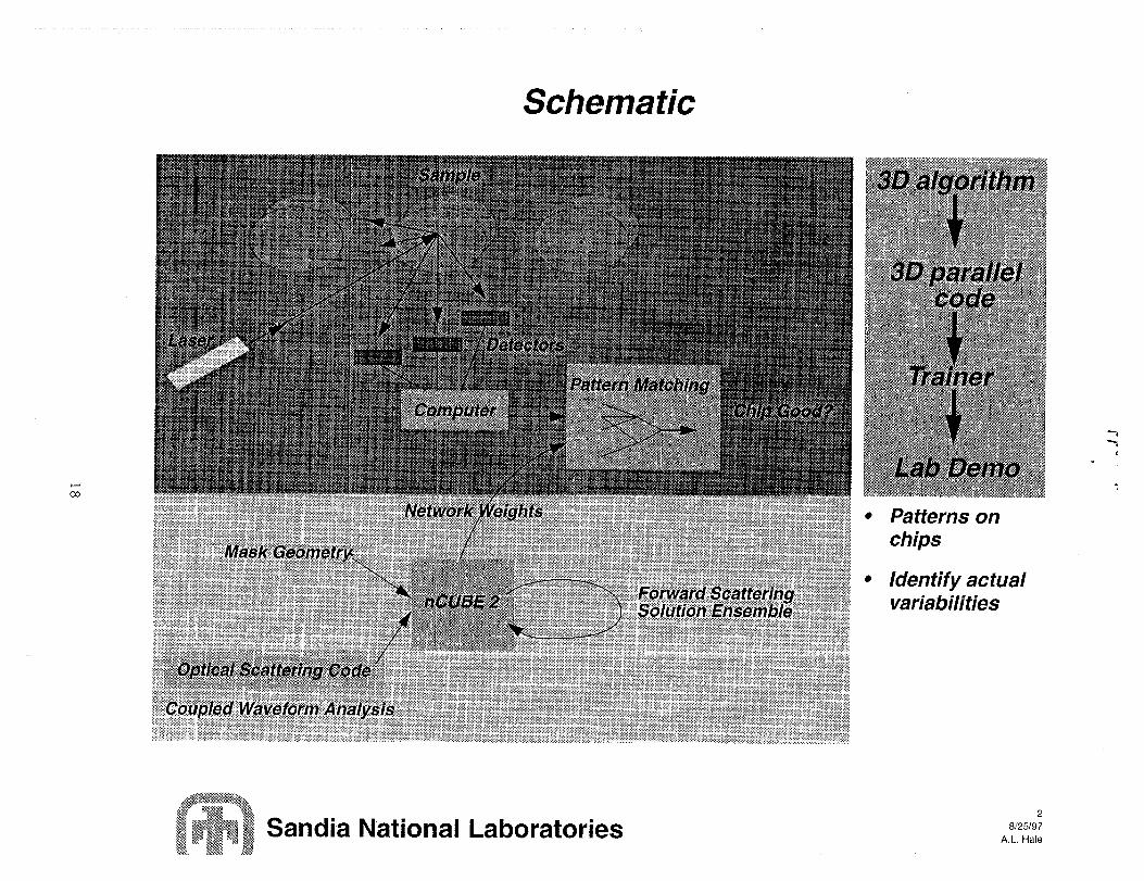
In subsequent discussion, we developed the following conceptual design for such
a system: A Computer Aided Design (CAD) mask far a new chip containing an ap-
propriate test pattern would be submitted to a large multiprocessing system (at, e.g.,
the MP CRL) and a concise list of a few hundred neural network training parameters
returned. These parameters would be fed into a small computer attached to a laser in-
terferometry apparatus which fired at each chip as it passed down the production line.
Chips that did not meet specification would be detected and rejected in real-time by
the small computer running a neural network pattern matching algorithm. Appendix 1
shows a schematic of the system corresponding to this conceptual design.At the end of the first year, we had passed the following milestones in
of this system:development
3
●
●
●
●
●
Designed in the MDL a mask for the special test chip required.
Adapted the code solving the 2D forward electromagnetic scattering code to
run in parallel on the Ncube2 hypercube multiprocessor with high parallel
efficiency and nearly perfect scalability.
Derived the appropriate 3D electromagnetic scattering equations (a significant
extension from the 2D case),
Implemented a pattern matching neural network which used the output of the
2D forward scattering code to solve the inverse scattering problem.
Compared the output of the neural network with that of a classical pattern
matching technique (linear least squares) and experimental results (from UNM’S
apparatus) and found excellent agreement,
Hence we deviated, as discussed previously, from the original plan in two important
ways:
●
●
We used a more straightforward parallelism than we originally planned in
adapting the 2D forward scattering code to the Ncube. This was more efficient
and natural in the 2D case, but it was not clear whether a similar simplification
would be possible in the 3D case.
We decided to investigate using a Multilayer Perception neural network to
implement the pattern matching algorithm. This approach was not mentioned
in the original proposal, and it was not clear that its use in solving the inverse
problem was justified. On simple problems the classical linear least squares
approach actually worked better. But the neural network approach offered an
attractive flexibility, and we felt that on more difficult or higher dimensional
geometries, it might also work better.
In the second year, we accomplished the following:
●
●
●
●
Fabricated a test chip from mask.
Implemented the 3D forward electromagnetic scattering equations in serial.
Converted the 3D serial code to run in parallel on the Ncube2.
Used the 3D forward scattering data to train and test the neural networkdesigned to solve the inverse problem.
Compared the neural network and classical results pattern matching algorithm
test results.
Verified the pattern matching code on the test chip.
The major developments here were:
We determined that the classical pattern matching technique was preferable to
the MLP neural network approach since it achieved comparable results more
simply and efficiently.
We showed that we were able to measure diffraction
accuracy comparable to the best previously existing
desirable because they are either invasive or require
grating parameters with
methods (which are less
human intervention and
4
hence are disruptive of production flow).
3. Technical Detail.
3.1. Improvements in RC WA Technique. The theory underlying our compu-
tational work is known as Rigorous Coupled Wave Analysis (RCWA) and is best laid
out by Moharam and Gaylord [5]. We describe several improvements and extensions
assuming their development and not ation.
The RC WA technique relies crucially on the computation of eigenvalues of a struc-
tured matrix and the solution of an associated linear system. Most of the compute time
is spent in either the eigensolve on the matrix A or the linear solve on the matrix Q.
Hence we tried to reduce the time spent in these kernels. We found four ways to do
this:
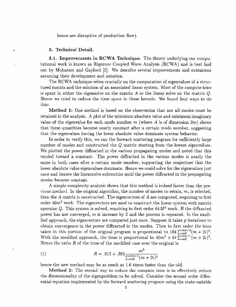
Method 1: One method is based on the observation that not all modes must be
retained in the analysis. A plot of the minimum absolute value and minimum imaginary
value of the eigenvalue for each mode number m (where A is of dimension 2m) shows
that these quantities become nearly constant after a certain mode number, suggesting
that the eigenvalues having the lower absolute value dominate system behavior.
In order to verify this, we ran the forward scattering program for sufficiently large
number of modes and constructed the Q matrix starting from the lowest eigenvalues.
We plotted the power diffracted in the various propagating modes and noted that this
tended toward a constant. The power diffracted in the various modes is nearly the
same in both cases after a certain mode number, supporting the conjecture that the
lower absolute value eigenvalues dominate. Hence we could solve for the eigenvalues just
once and iterate the linearsolve subroutine until the power diffracted in the propagating
modes became constant.
A simple complexity analysis shows that this method is indeed faster than the pre-vious method. In the original algorithm, the number of modes to retain, m, is selected,
then the A matrix is constructed, The eigenvectors of A are computed, requiring to first
order 40m3 work. The eigenvectors are used to construct the linear system with matrix
operator Q. This system is solved, requiring to first order 64.M3 work. If the diffracted
power has not converged, m is increase by 2 and the process is repeated. In the modi-
fied approach, the eigenvectors are computed just once. Suppose it takes p iterations to
obtain convergence in the power diffracted in the modes. Then to first order the time
taken in this portion of the original program is proportional to 104 ~~~~-l(m + 2i)3.
With the modified approach, the time is proportional to 40m3 + 64 ~~~~-1 (m + 2i)3.
Hence the ratio R of the time of the modified case over the original is
(1) R = .615+ .385 ._m’
~~~~-l(m + 2i)3
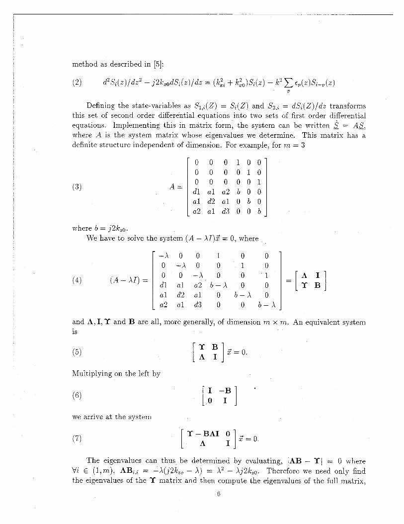
hence the new method may be as much as 1.6 times faster than the old.Method 2: The second way to reduce the compute time is to effectively reduce
the dimensionality of the eigenproblem to be solved. Consider the second order differ-ential equation implemented by the forward scattering program using the state-variable
Defining the state-variables as S1,i(Z) = SZ(Z) and S2,i = cLS’i(Z)/dz transforms
this set of second order differential equations into two sets of first order differential
equations. Implementing this in matrix form, the system can be written 1 = AS’,
where A is the system matrix whose eigenvalues we determine. This matrix has a
definite structure independent of dimension. For example, for m = 3
(3)
[
000100000010
A=000001
dlala2b O0
[
ald2a1060
a2ald300b
where b = j2kzo.
We have to solve the system (A – Af)Z = O, where
–Ao o 1 0 00 –Ao o 1 0
(4)–A o 0 1
(A - AI)= ;1 :1 [1AI
(z2 b–~ O 0 ‘YBal d2 al O b–~ O
a2 al d3 O 0 b–~
and A, 1, Y and B are all, more generally, of dimension m x m. An equivalent system
is
(5)
Multiplying on the left by
(6)
we arrive at the system
[1T B ;=O
AI.
HI–B’
01
[
Y–BAI O 1(7)A I ‘=O.
The eigenvalues can thus be determined by evaluating, IAB – T\ = O where
Vi E (l, m), ABi,; = –A(j2kzo – A) = A’ – Aj2k,o. Therefore we need only find
the eigenvalues of the Y matrix and then compute the eigenvalues of the full matrix,
6
A, using the quadratic formula ~2 – Aj2kz0 – q = O where al is the lt~ eigenvalue of
the Y matrix, i.e.
Hence we have effectively halved the dimensionality of the eigenproblem to be solved.
Since this is a cubic operation, this saves us about a factor of 8 in work associated with
solving the eigenproblem.
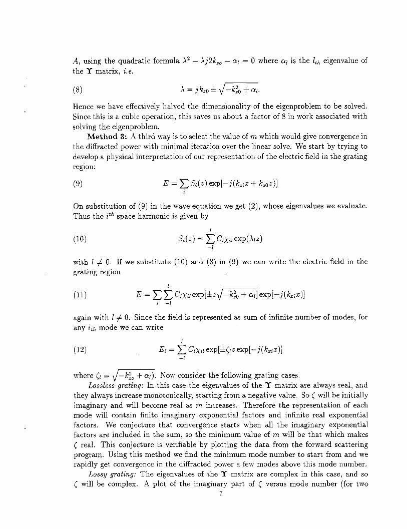
Method 3: A third way is to select the value of m which would give convergence in
the diffracted power with minimal iteration over the linear solve. We start by trying todevelop a physical interpretation of our representation of the electric field in the grating
region:
(9) E = ~ Si(z) exp[–j(k.iz + kzoz)]i
On substitution of (9) in the wave equation we get (2), whose eigenvalues we evaluate.
Thus the it~ space harmonic is given by
with 1 # O. If we substitute (10) and (8) in (9) we can write the electric field in the
grating region
(11) E = ~ ~ Clxil exp[+z~-exp[–j( k=iz)]i —/
again with Z# O. Since the field is represented as sum of infinite number of modes, for
any ith mode we can write
where cl = m Now consider the following grating cases.
Loss/ess grating: In this case the eigenvalues of the Y’ matrix are always real, and
they always increase monotonically, starting from a negative value. So ~ will be initially
imaginary and will become real as m increases. Therefore the representation of each
mode will cent ain finite imaginary exponential factors and infinite real exponential
factors. We conjecture that convergence starts when all the imaginary exponential
factors are included in the sum, so the minimum value of m will be that which makes
< real. This conjecture is verifiable by plotting the data from the forward scattering
program. Using this method we find the minimum mode number to start from and we
rapidly get convergence in the diffracted power a few modes above this mode number.
Lossy grating: The eigenvalues of the T matrix are complex in this case, and so~ will be complex. A plot of the imaginary part of ~ versus mode number (for two
7
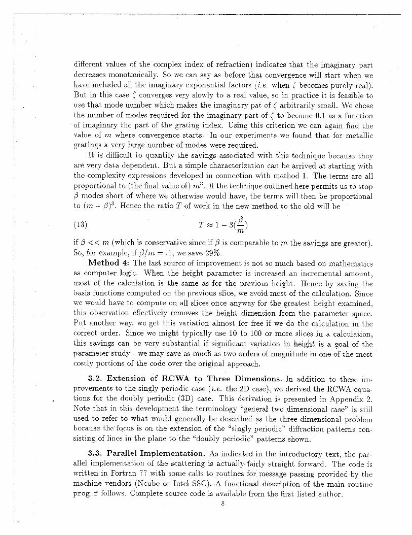
different values of the complex index of refraction) indicates that the imaginary part
decreases monotonically. So we can say as before that convergence will start when we
have included all the imaginary exponential factors (i. e. when ~ becomes purely real).
But in this case ( converges very slowly to a real value, so in practice it is feasible to
use that mode number which makes the imaginary pat of [ arbitrarily small. We chose
the number of modes required for the imaginary part of ~ to become 0.1 as a function
of imaginary the part of the grating index. Using this criterion we can again find the
value of m where convergence starts. In our experiments we found that for metallic
gratings a very large number of modes were required.
It is difficult to quantify the savings associated with this technique because they
are very data dependent. But a simple characterization can be arrived at starting with
the complexity expressions developed in connection with method 1. The terms are all
proportional to (the final value of) m 3. If the technique outlined here permits us to stop
/3 modes short of where we otherwise would have, the terms will then be proportional
to (m – /?)3. Hence the ratio T of work in the new method to the old will be
(13) T%l–3(:)
if ~ << m (which is conservative since if @ is comparable to m the savings are greater).
So, for example, if ~/m = .1, we save 29%.
Method 4: The last source of improvement is not so much based on mathematics
as computer logic. When the height parameter is increased an incremental amount,
most of the calculation is the same as for the previous height. Hence by saving thebasis functions computed on the previous slice, we avoid most of the calculation. Sincewe would have to compute on all slices once anyway for the greatest height examined,
this observation effectively removes the height dimension from the parameter space.
Put another way, we get this variation almost for free if we do the calculation in the
correct order. Since we might typically use 10 to 100 or more slices in a calculation,
this savings can be very substantial if significant variation in height is a goal of the
parameter study - we may save as much as two orders of magnitude in one of the most
costly portions of the code over the original approach.
3.2. Extension of RCWA to Three Dimensions. In addition to these im-provements to the singly periodic case (i.e. the 2D case), we derived the RCWA equa-
tions for the doubly periodic (3D) case. This derivation is presented in Appendix 2.
Note that in this development the terminology “general two dimensional case” is still
used to refer to what would generally be described as the three dimensional problembecause the focus is on the extension of the “singly periodic” diffraction patterns con-
sisting of lines in the plane to the “doubly periodic)’ patterns shown.
3.3. Parallel Implementation. As indicated in the introductory text, the par-
allel implementation of the scattering is actually fairly straight forward. The code is
written in Fortran 77 with some calls to routines for’ message passing provided by the
machine vendors (Ncube or Intel SSC). A functional description of the main routine
prog. f follows. Complete source code is available from the first listed author.8
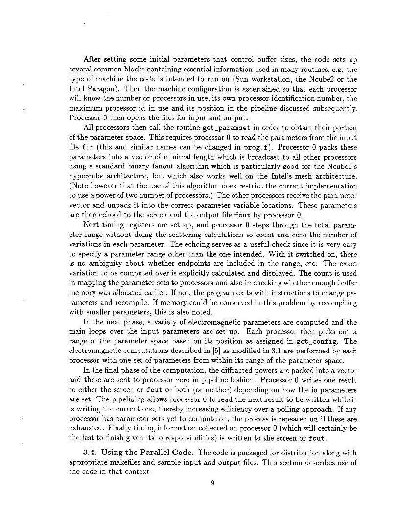
After setting some initial parameters that control buffer sizes, the code sets up
several common blocks containing essential information used in many routines, e.g. the
type of machine the code is intended to run on (Sun workstation, the Ncube2 or the
Intel Paragon). Then the machine configuration is ascertained so that each processorwill know the number or processors in use, its own processor identification number, the
maximum processor id in use and its position in the pipeline discussed subsequently.
Processor O then opens the files for input and output.
All processors then call the routine get-paramset in order to obtain their portion
of the parameter space. This requires processor O to read the parameters from the input
file fin (this and similar names can be changed in prog. f ). Processor O packs these
parameters into a vector of minimal length which is broadcast to all other processors
using a standard binary fanout algorithm which is particularly good for the Ncube2’s
hypercube architecture, but which also works well on the Intel’s mesh architecture.
(Note however that the use of this algorithm does restrict the current implementation
to use a power of two number of processors.) The other processors receive the parameter
vector and unpack it into the correct parameter variable locations. These parameters
are then echoed to the screen and the output file fout by processor O.
Next timing registers are set up, and processor O steps through the total param-
eter range without doing the scattering calculations to count and echo the number of
variations in each parameter. The echoing serves as a useful check since it is very easy
to specify a parameter range other than the one intended. With it switched on, there
is no ambiguity about whether endpoints are included in the range, etc. The exactvariation to be computed over is explicitly calculated and displayed. The count is used
in mapping the parameter sets to processors and also in checking whether enough buffer
memory was allocated earlier. If not, the program exits with instructions to change pa-
rameters and recompile. If memory could be conserved in this problem by recompiling
with smaller parameters, this is also noted.
In the next phase, a variety of electromagnetic parameters are computed and the
main loops over the input parameters are set up. Each processor then picks out a
range of the parameter space based on its position as assigned in get -conf ig. The
electromagnetic computations described in [5] as modified in 3.1 are performed by each
processor with one set of parameters from within its range of the parameter space.
In the final phase of the computation, the diffracted powers are packed into a vector
and these are sent to processor zero in pipeline fashion. Processor O writes one result
to either the screen or fout or both (or neither) depending on how the io parameters
are set. The pipelining allows processor O to read the next result to be written while it
is writing the current one, thereby increasing efficiency over a polling approach. If any
processor has parameter sets yet to compute on, the process is repeated until these are
exhausted. Finally timing information collected on processor O (which will certainly be
the last to finish given its io responsibilities) is written to the screen or fout,
3.4. Using the Parallel Code. The code is packaged for distribution along with
appropriate makefiles and sample input and output files. This section describes use of
the code in that context
9
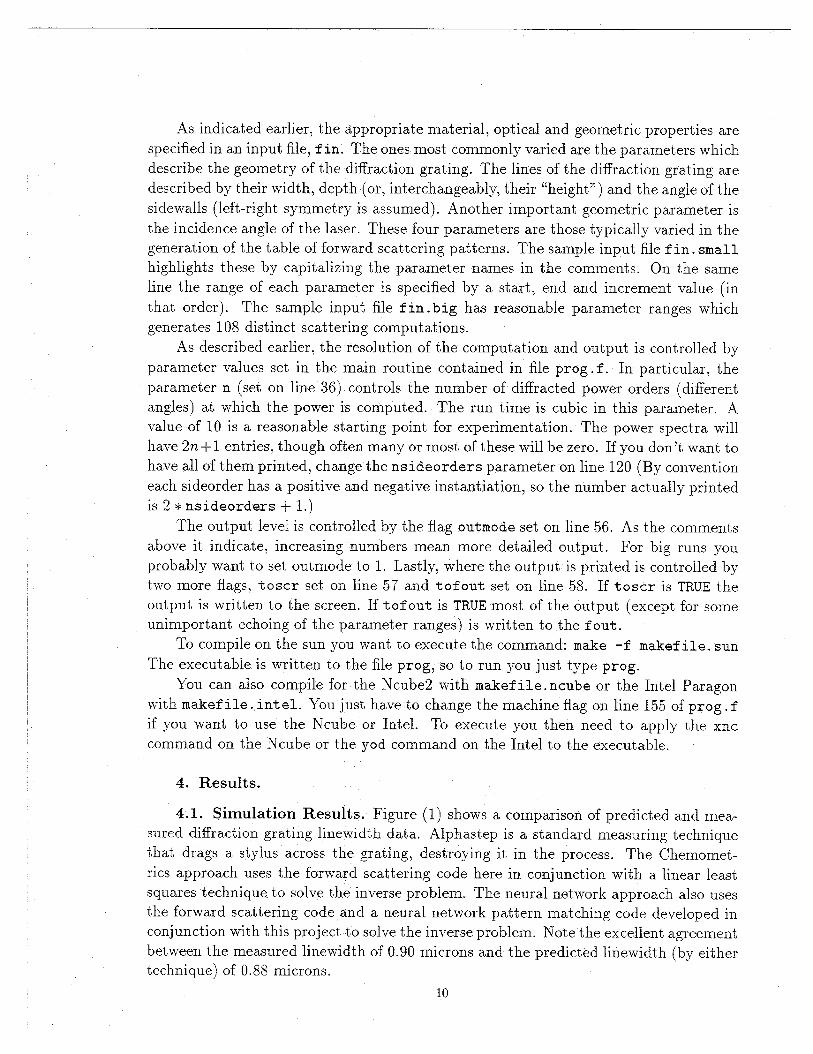
As indicated earlier, the appropriate material, optical and geometric properties are
specified in an input file, fin. The ones most commonly varied are the parameters which
describe the geometry of the diffraction grating. The lines of the diffraction grating are
described by their width, depth (or, interchangeably, their “height”) and the angle of the
sidewalls (left-right symmetry is assumed). Another important geometric parameter is
the incidence angle of the laser. These four parameters are those typically varied in the
generation of the table of forward scattering patterns. The sample input file f in. small
highlights these by capitalizing the parameter names in the comments. On the same
line the range of each parameter is specified by a start, end and increment value (in
that order). The sample input file fin. big has reasonable parameter ranges which
generates 108 distinct scattering computations.
As described earlier, the resolution of the computation and output is controlled by
parameter values set in the main routine cent ained in file prog. f. In particular, the
parameter n (set on line 36) controls the number of diffracted power orders (different
angles) at which the power is computed. The run time is cubic in this parameter. Avalue of 10 is a reasonable starting point for experimentation. The power spectra will
have 2n+ 1 entries, though often many or most of these will be zero. If you don’t want to
have all of them printed, change the nsideorders parameter on line 120 (By convention
each sideorder has a positive and negative instantiation, so the number actually printed
is 2 * nsideorders + 1.)
The output level is controlled by the flag outmode set on line 56. As the comments
above it indicate, increasing numbers mean more detailed output. For big runs you
probably want to set outmode to 1. Lastly, where the output is printed is controlled bytwo more flags, toscr set on line 57 and tofout set on line 58. If toscr is TRUEthe
output is written to the screen. If tofout is TRUEmost of the output (except for some
unimportant echoing of the parameter ranges) is written to the f out.
To compile on the sun you want to execute the command: make -f makef i.le. Sun
The executable is written to the file prog, so to run you just type prog.
You can also compile for the Ncube2 with makef ile. ncube or the Intel Paragon
with makef ile .,int el. You just have to change the machine flag on line 155 of prog. f
if you want to use the Ncube or Intel. To execute you then need to apply
command on the Ncube or the yod command on the Intel to the executable.
4. Results.
the xnc
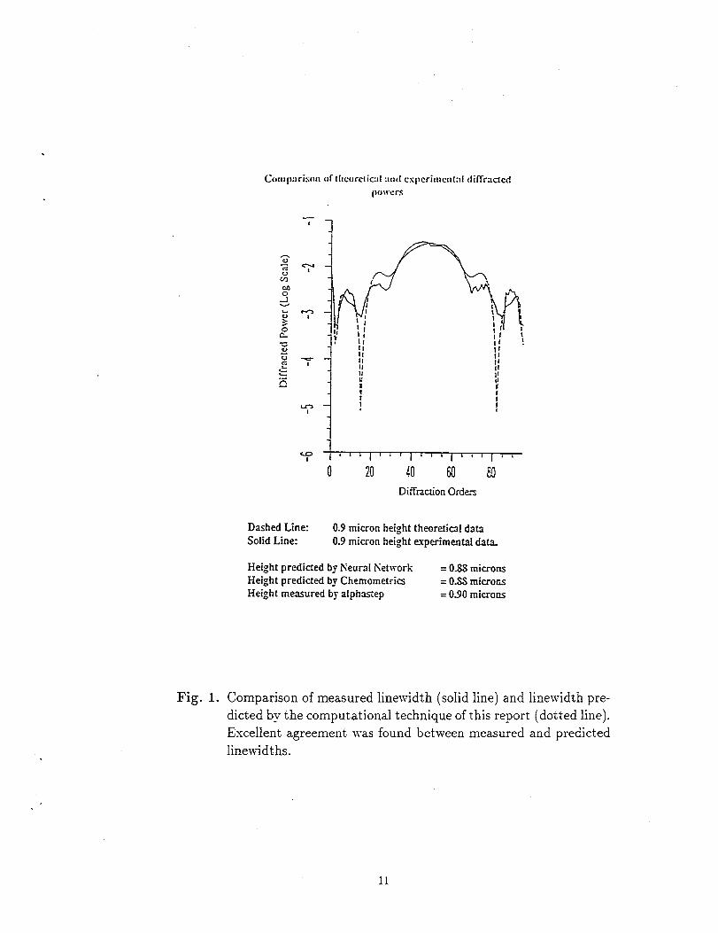
4.1. Simulation Results. Figure (1) shows a comparison of predicted and mea-
sured diffraction grating linewidth data. Alphastep is a standard measuring technique
that drags a stylus across the grating, destroying it in the process. The Chemomet-
rics approach uses the forward scattering code here in conjunction with a linear least
squares technique to solve the inverse problem. The neural network approach also uses
the forward scattering code and a neural network pattern matching code developed in
conjunction wit h this project to solve the inverse problem. Note the excellent agreement
between the measured linewidth of 0.90 microns and the predicted Iinewidth (by either
Height predicted by Neural Network = 0.SS micronsHeight predickd by Chemometria = 0.SSmicroosHeight measured by alphastep = 0.90 microns
Fig. 1. Comparison of measured linewidth (solid line) and Iinewidt h pre-
dicted by the computational technique of this report (dotted line).
Excellent agreement was found between measured and predicted
Iinewidths.
11
Ncube: Fxed Problem
1OQoo
z
:i=
5000
00 Too 200 3(KI 400 500 600 700 800 WI 100
Number Processors
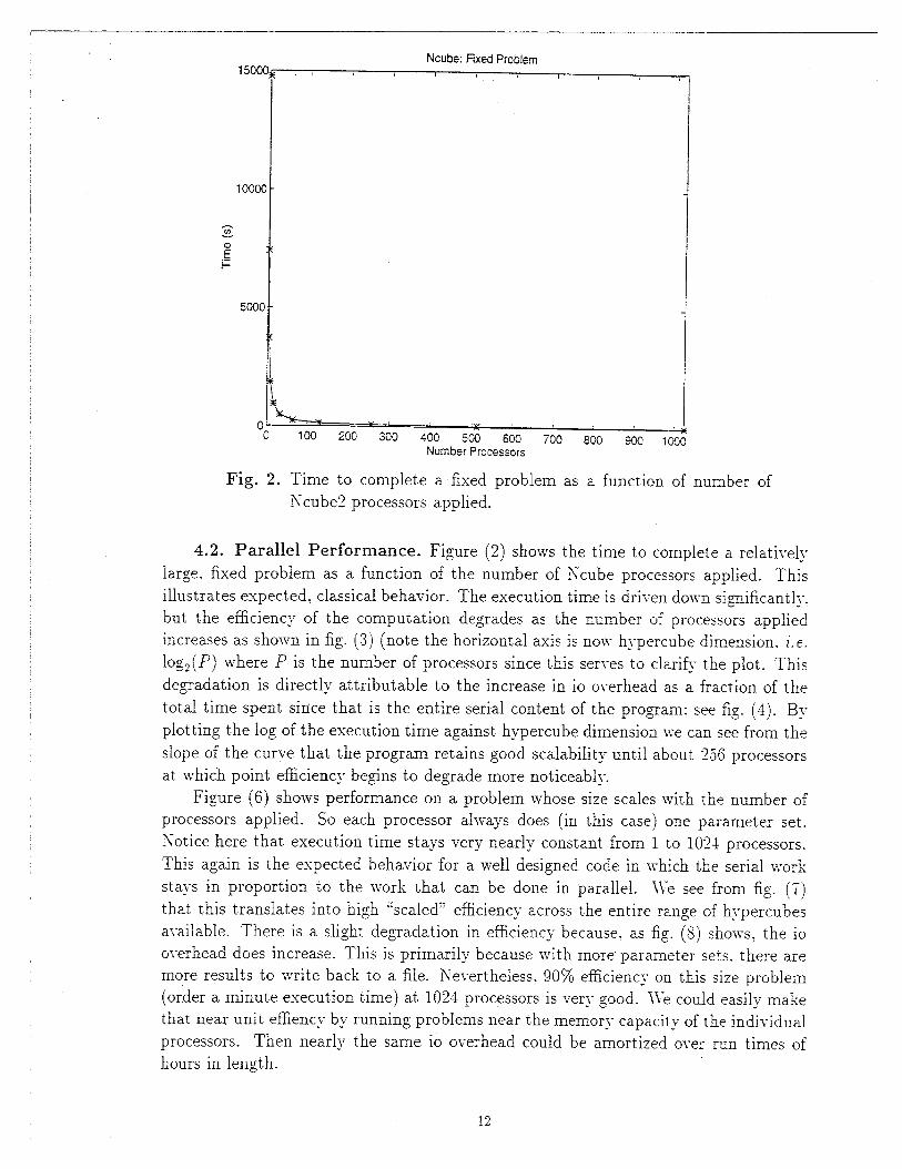
Fig. 2. Time to complete a fixed problem as a function of number of
Xcube2 processors applied.
4.2. Parallel Performance. Figure (2) shows the time to comple~e a relatively
large, fixed problem as a function of the number of Ncube processors applied. This
illustrates expected, classical behavior. The execution time is dri~en down si=mificantly,
but the efficiency of the computation degrades as the number of processors applied
increases as shown in fig. (3) (note the horizontal axis is now h~-percube dimension. i.e.
logz(P) where P is the number of processors since this ser~es to clarify the plot. This
degradation is directly attributable to the increase in io o~-erhead as a fraction of the
total time spent since that is the entire serial content of the pro~am; see fig. (4). By
plotting the log of the execution time against hypercube dimension we can see from the
slope of the curve that the program retains good scalability until about 2.56 processors
at. which point efficiency begins to degrade more noticeably.
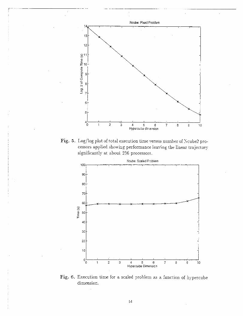
Figure (6) shows performance on a problem whose size scales with the number of
processors applied. So each processor always does (in this case) one parameter set.
Xotice here that execution time stays very nearly constant from 1 to 1024 processors.
‘This again is the expected behavior for a well designed code in which the serial work
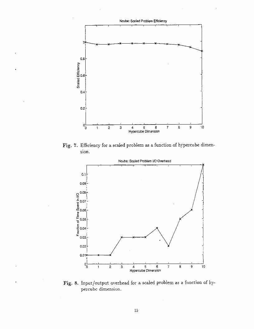
stays in proportion to the work that can be done in parallel. l\’e see from fig. (7)
that this translates into high “scaled” efficiency across the entire range of hypercubes
a~-ailable. There is a slight degradation in efficiency because. as fig. (S) shows? the io
o~erhead does increase. This is primarily because with more parameter sets. there are
more results to write back to a file. hTevertheless, 90’70 efficiency on this size problem
(order a minute execution time) at 1024 processors is very good. Jf:e could easily make
that near unit effiency by running problems near the memor~- capacity of The individual
processors. Then nearly the same io overhead could be amortized over run times of
hours in length.
12
.
Ncu!w Fxed Problem Effkiamy
[
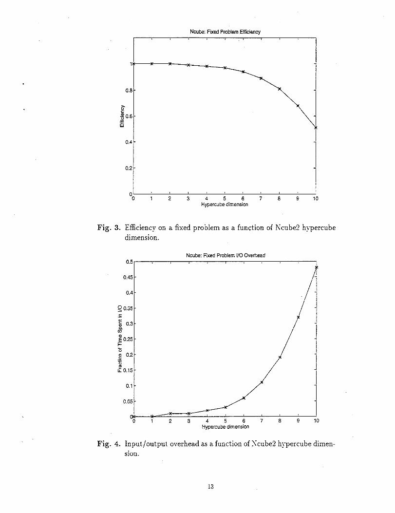
Fig. 3.
01 ‘ ‘ , f
o 1 2345678 $1;Hyperwce dimmsion
Efficiency on a fixed problem as a function of Ncube2 hypercube
dimension.
Ncube Fxed Problem i/O Overhead0.5 k , & 8
0.45 -/
0.4
I~ 0.35 j-~ I
g 0.3 -I
%; 0.25 -
1
i=z ]g 0.2 -=u
z 0.15 -
0.1 -
0.05 -
wo 1 2 3 4 5 678 Q 10
Hypercube dimension
Fig. 4. Input/output overhead as a function of Jcube2 hypercube dimen-
sion.
13
Ncu& Fixed Problem
Fig. 5.
1
K“”13
12
‘o 1 2 3 A 5 6 7 8 ~ 10Hypercube dimension
Log/log plot of total execution time versus number of Xcube2 pro-
cessors applied showing performance leaving the linear trajectory
significantly at about 2.56 processors.
100
90
80
70
60
50
40
30
20
10
Ncube: Scaled Problem
[ 1I
o , ,0 1 2 3 4 5 6 7 8 9 10
Hypercube Dimension
Fig. 6. Execution time for a scaled
dimension
14
function of hypercube
Ncubet Sceled Problem E?ficisncy
I
0.8 }
0.4
0.2 1
o~ ‘ ‘ ‘ I
01 2345678 910Hyprcube Dimension
Fig. 7. Efficiency for a scaled problem as a function of hypercube dimen-
sion.
Ncube: Scaled Problem l/O Overhead, c
0.1-
0.09 -
~ 0.08 -:
:0.07 -al
/~ o.06 -
g
; 0.05 -
g 0.04 -~
u 0.03 -,
x q{0.02 -
o.ol~ (
01 ! r , I
o 1 2 3 4 5 6 7 8 g 10Hypercube Dimension
Fig. 8. Input/output overhead for a scaled problem as a function of hy-percube dimension.
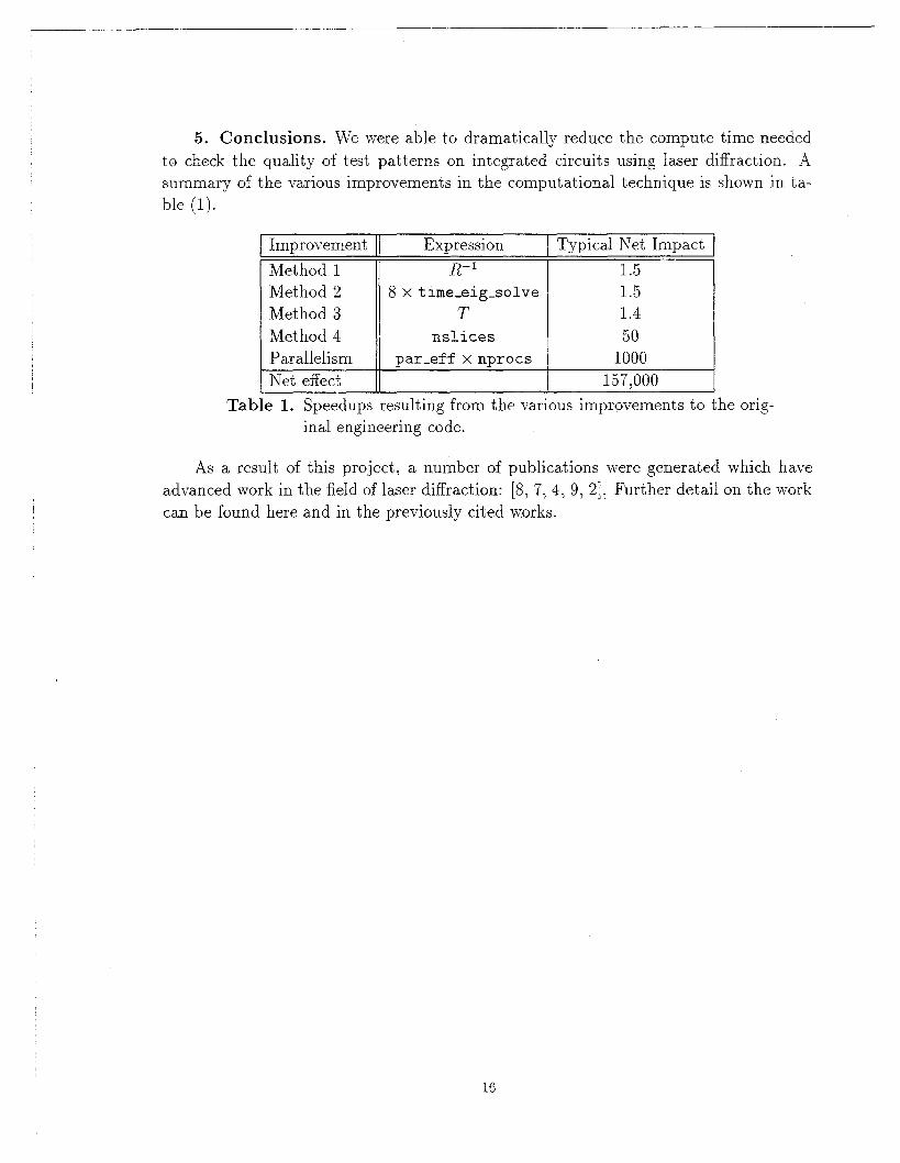
5. Conclusions. We were able to dramatically reduce the compute time needed
to check the quality of test patterns on integrated circuits using laser diffraction. A
summary of the various improvements in the computational technique is shown in ta-
ble (1).
Tab
Improvement
Method 1
Method 2
Method 3
Method 4
Parallelism
Net effect
Expression I Typical Net ImpactR-1 1.5
8 x time.eig-solve 1.5
T 1.4
nslices 50par.eff x nprocs 1000
157,000
>1. Speedups resulting from the various improvements to the orig-inal engineering code.
As a result of this project, a number of publications were generated which have
advanced work in the field of laser diffraction: [8, 7, 4, 9, 2]. Further detail on the work
can be found here and in the previously cited works.
16
REFERENCES
[1] K. C. HICKMAN, S. S. GASPAR, S. S. NAQVI, K. P. BISHOP, J. R. MCNEIL, G. D. TIPTON,B. L. DRAPER, AND B. R. STALLARD, Use of diffraction from latent images to improve/i-thography control, Integrated Circuit Metrology, Inspection and Process Control V, SPIE1464 (1991).
[2] R. KRUKAR, R. W. LELAND, AND S. R. MCNEIL, Determining the limit for diffraction basedmetrology, in Machine Vision Applications in Industrial Inspections II, SPIE Symposium onElectronic Imaging Science and Technology, February 1994.
[3] R. W. LELAND, The Effectiveness of Paraliel Iterative Algorithms for Solution of Large SparseLinear Systems, PhD thesis, University of Oxford, Oxford University Computing Laboratory,Oxford, England, October 1989.
[4] B. MINHAS, S. S. NAQVI, ANDR. W. LELAND,A study of eigenvalue behavior in rigorous coupledwave analysis, in Optical Society of America Annual Meeting, October 1993.
[5] M. G. MOHARAM AND T. K. GAYLORD, Diffraction analysis of dielectric surface-relief gratings,Journal of the Optical Society of America, 72 (1982), pp. 1385-1392.
[6] S. S. NAQVI, S. M. GASPAR, K. C. HICKMAN, AND J. R. MCNEIL, A simple technique forlinewidth measurement of gratings on photomasks, Integrated Circuit Metrology, Inspectionand Process Control IV, SPIE 1261 (1990), pp. 495-504.
[7] S. S. NAQW AND R. W. LELAND, Massively parallel solution of scattering from doubly periodicstructures, in Optical Society of America Annual Meeting, 1992.
[8] S. S. NAQVI, J. R. MCNEIL, R. KRUKAR, FRANCO, R. W. LELAND, AND K. P. BISHOP, Firstprinciple simulation of diffraction based metrology techniques, Microelectronics World, (1993).
[9] S. S. NAQVI, B. MINHAS, R. KRUKAR, AND R. W. LELAND, Electromagnetic scattering analysisof diffraction gratings, in Optical Society of America Annual Meeting, October 1993.
17
Schematic
Sandia National Laboratories
● Patterns onchips
● Identify actualvariabilities
28/25/97
AL, Hale
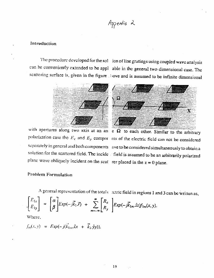
Itllrudt-lclion
‘llw pmccdurc tievcloped forthe so]
cnn he conveniently extended to be appl
scattering sufiace is, given in the figLIre
ion olline gratings using coupled wave analysis
ab~e in U-Egeneral two dimension case. The
love and is assumed to be infinite dimensional
. .W’IUI apertures along [wu axis tit an an:
polarization case the If< Hnclfly Compor
scpnr:t!ely in general aIId Im[h components
e U to each other. Similar to the arbitrary
IILSof the dcct.ic field can not bc considered
ave to be considered sinmltw~eously to obtain aSOILItion fm the scattered field. The incidc I fielcl is assunled LObe an arbitrarily polarized
i)I:inc Ivavc c)hliqLlclyincident on the scat’
ProldcIn Fmmllllalif)n
A :cneril rcprescnt;~[ion ufthe mtul (
rer placed in the z = Oplane.
:ctric field in regions 1 and 3 can be writlcn as,
IExp(- j&.2),fl#, y).
W’llcl”e.
J,,(x.-v) = Exp(-.j(i’i,,t..ix+ 11.jy)).
*
19
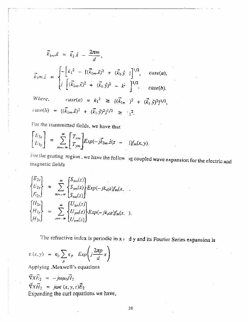
kl,,li 2Jrm= i-’..; – —
d’
l:or [hc ~r:tnsmitt.ed f-iclds, we have that
‘=-= [52,,1(Z)J
“1’hc refractive index is periodic in x i d y and its Fourier Series expansion is
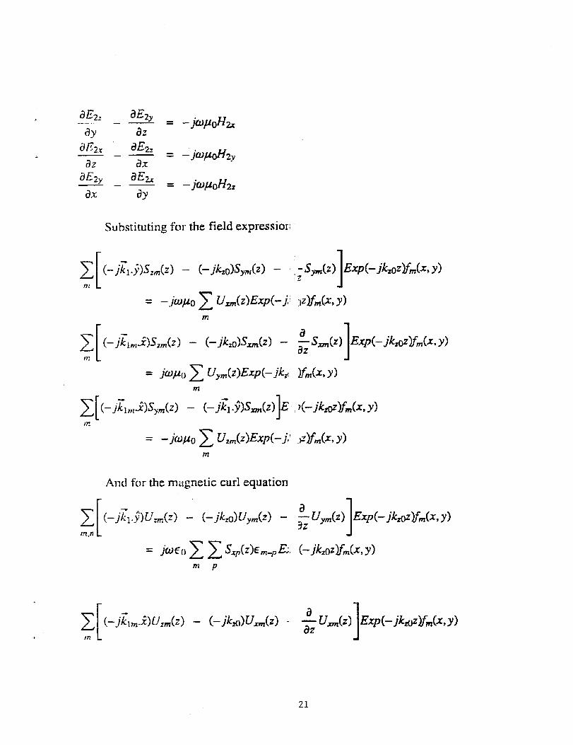
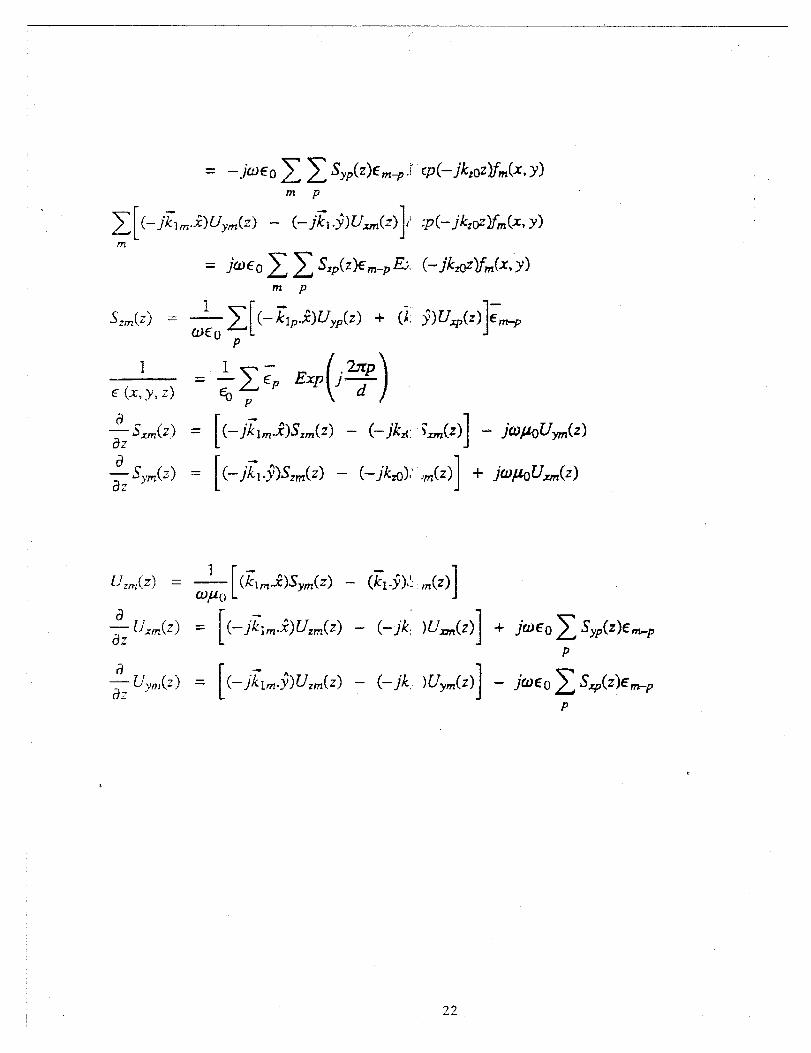
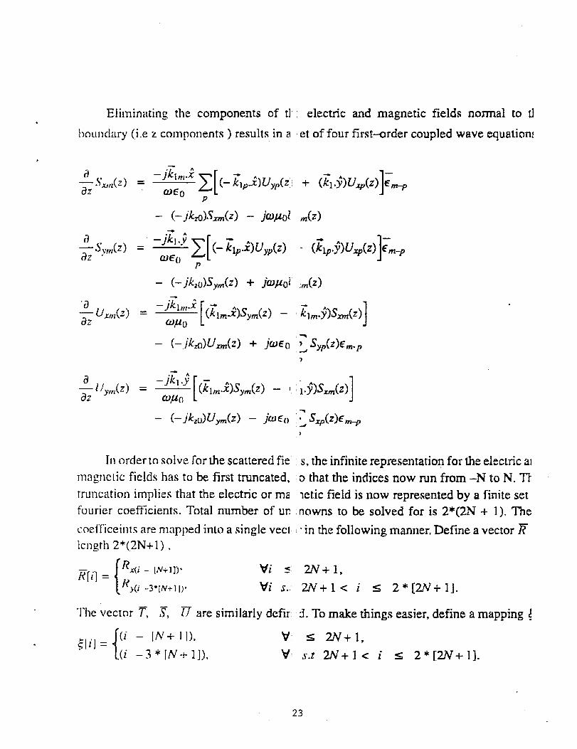
Eliminating the components of t] : electric and magnetic fields normal to tl
Imunclary (,i.e z components ) results in a et of four first-order coupled wave equation!
– (- jkfi).$m(z) – ja.yd ,Jz)
+ Sy,,,(z) =– jZ, .j ~[(-&wJyp(z)
1- (Zip.jw.p(z) G-p
CLE()P
- (–)’kzd$nt(d + ju/foi” m(z).
: Urn(z) = ‘Jk~,t,.x [(L?#)sym(4– Lm?n(z)
quo 1–(–.PLWA) + j@~O ‘~ ~yp(z)~m.p
-)
: Uy,,,(z) =[
‘“~kl“;(I,mt.i)sym(z)- ‘ ~l.;)%(z)~ cop[) 1
–(–j&)Uy~(z)–j~~[}~~SV(Z)E”,~#
In order m solve for fie sca~tered fie s, the infinite representatioIl for the electric a]
magnc[ic fields has to be first truncated, o that the indices now run from –N to N. Tl
mmcation implies that the electric or ma wtic field is now represented by a finite setfburier coefficients. Total number of un nowns to be solved for is 2*(2N + 1). The
coc.f’f.ic.ein~.sare mapped into a single vect ~-in the following manner, Define a vector ~kngrh 2*(,2N+1 ) ,
{
R x(i - [h’+]])’ vi ~F[i] =
/’/y(i _~*lN+, ,), Vi s..
The vector ~, ~, ~ are similarly defir:
$Ii] ={
(i - [N+ll), v’
(i -3*[N-FIJ), v’
2N+1,
W+l< i 5 2*[21V+ I].
5. To make things easier, define a mapping ~
s 2N+1,
,S.t 2N+1C i s 2*[2N+ 1].
23
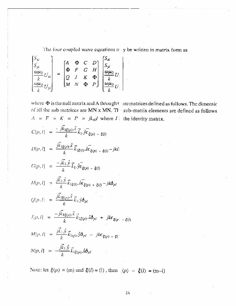
‘1’lw f(mr CXmpkd wave equations n
s’
1[A@c~~’:@F GHy’
y[l:Q,IKcD.
where @ is Ihe IILIll nlftlrix aIIclA through (
—
y be wrilten in remix foml as
:IIYJmatrices defined as follows. The dimensir
sub-matrix eIemenG are defined tis follows
[he ident.ity matrix.
- $?(I)
(y) - $(l) = (m-i)
24
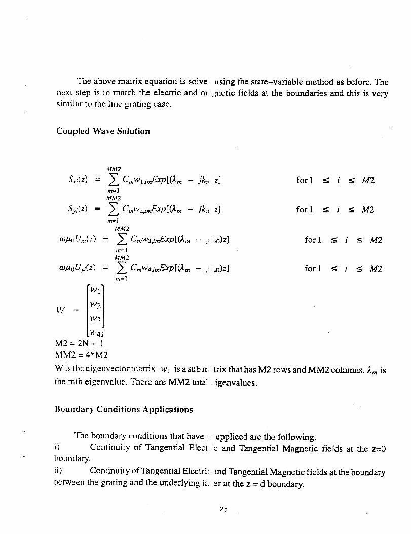
‘1’lIe above mit~rix equation is solve; using the state-variable method as before. “Ikenext step is LOmatch the electric and m; ,~etic fields at the boundaries and this is verysimilar tu the line grating case.
,
Coupled Wave Solution
MA42
&’i’~i(Z) =
JSyi(Z) =
(0/4( ) ‘V,~i(Z)In=lMM2
W is the cigenvec[or Il]atrix. w] is a sub n [rix that has M2 rows and MM2 columns. Amis
the mth eigenvaluc. There are TvlM2total t igenvalues.
Boundary Conditions Applications
.The boundary c[mditions that have I tipplieed are the fo]lowing.
i) Continuity of Tangential Elect c and Tangential Magnetic fields at the z=O* Ix)llndary.
ii) Continuity of “Ilmgential Electri: md Tangential Magnetic fields at the boundarybetween the grwing and the underlying k m at the z = d boundary.
25
26
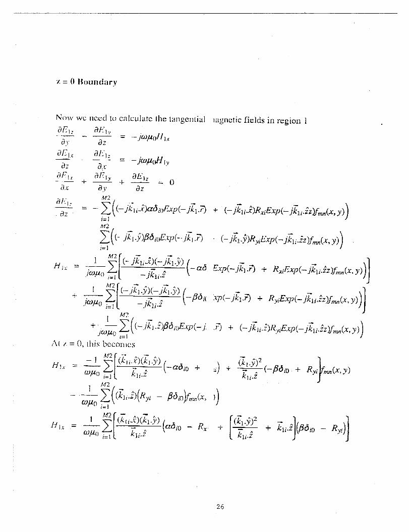
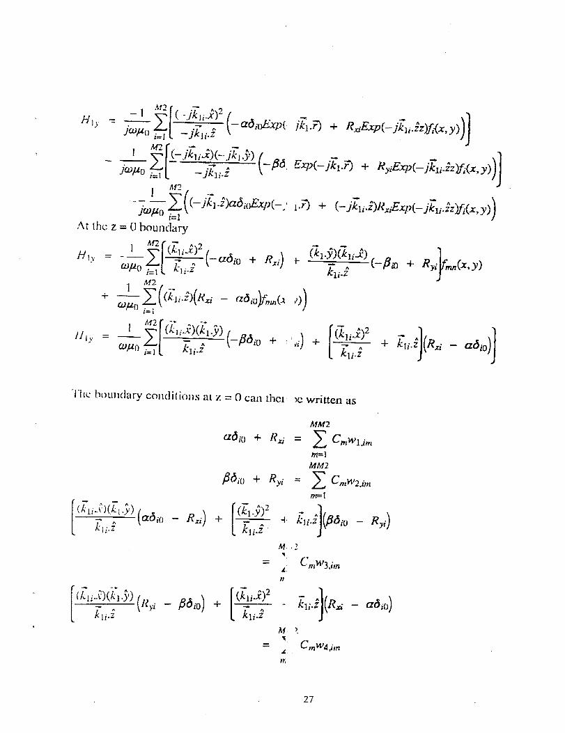
At (hc z = (1 hrmnd:iry
MM2
Udi(]+ Rm. = z CWIM’ljm
m=1A4M2
27
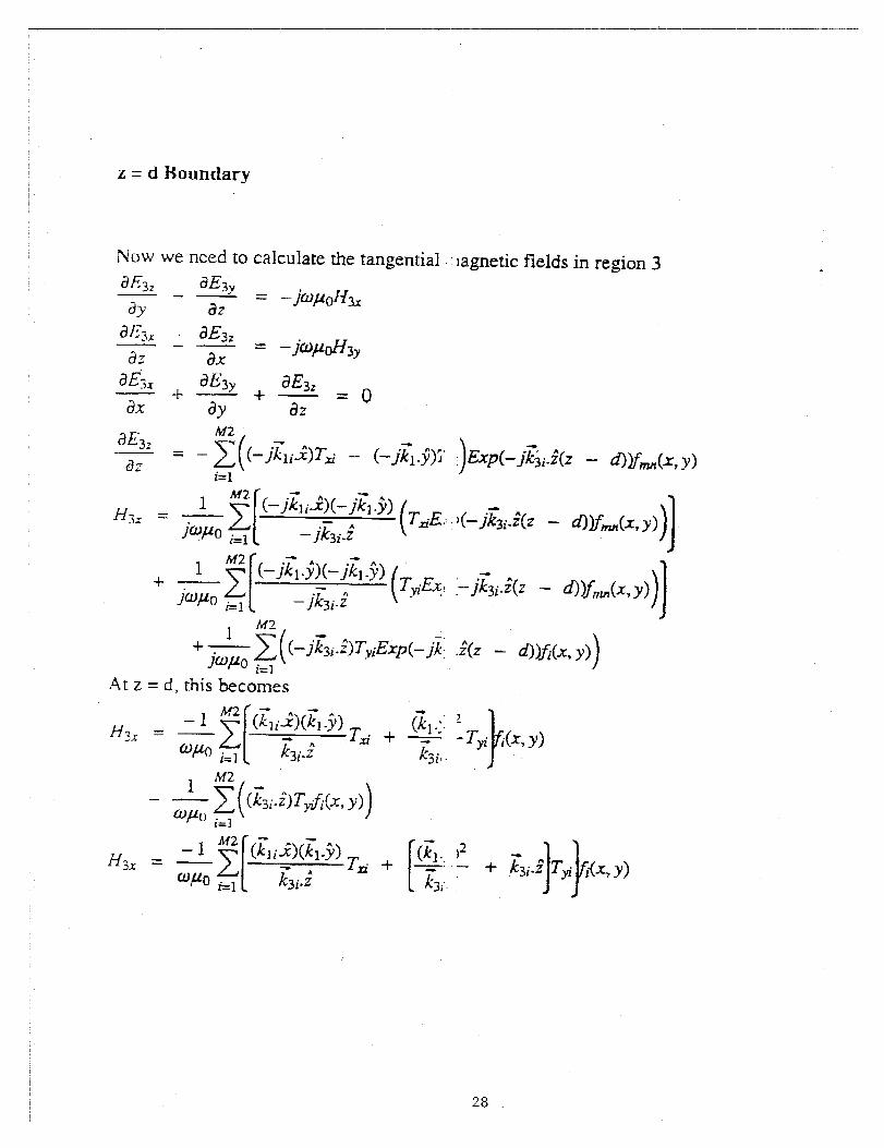
z = d Boundary
Now we need to calculate the tangential lagnetic fields in region 3 .aE3,— _ay