PAD5700 week three

Page 1 of 13

MASTER OF PUBLIC ADMINISTRATION PROGRAM

PAD 5700 -- Statistics for public management Fall 2013

Sampling and confidence intervals

Statistic of the week

√ ̅

The standard deviation

*

We start with some discussion of data gathering. There is an old cliché in statistics (or any sort

of analytical process) that if you put 'junk' in, you will get 'junk' out.

Think of the recent collapse of the US economy, and as a result global economy: no one

(effectively, click here and here for exceptions) saw it coming. The Bush administration's 2009

budget, for instance, was released early in 2008. In the Budget Message, the President

confidently stated that "As we enter this New Year, our economy retains a solid foundation

despite some challenges, revenues have reached record levels, and we have reduced the Federal

deficit by $250 billion since 2004." In Table S-10 of the Summary Tables, the administration

foresaw economic growth ('Real GDP' in the table) of 2.7% in 2008, followed by 3.0% growth in

2009. It wasn't just the Bush administration that was delusional. As this table also indicated, the

CBO (Congressional Budget Office, widely respected as a competent, and unbiased referee in

budget debates) expected growth of 1.7% and 2.8% for these two years, while the 'Blue Chip

consensus' (the mean prediction of a number of highly respected private economic forecasters)

was about halfway between the two. The actual result for 2008 was 1.0% growth, while 2009

saw about a 3.5% contraction in the economy.

Why? Because the data that they plugged into their economic models was faulty. While

numbers can be a very good way to describe reality (as we saw last week), statistics can be very

bad at prediction, and even worse at predicting unprecedented events. The logic of statistics is

that you plug past data into a dataset, develop a model to analyse it, then punch 'run'. It spits out

a result. However if the future diverges sharply from the past -- if something fundamental

changes -- by definition your past data will not have incorporated this. Indeed, even your model

can be wrong.

These same problems can occur even if the future doesn't reflect a break from the past, but the

analyst fails to sample the data correctly. Imagine conducting a survey about voting preferences

of Americans. If you hung out at Ponte Vedra and asked passersby you'd probably get a different

result than if you hung out on the east side of Jacksonville. For two similar examples: how would

you react if I told you that:

1. I played top 20 college hoops?

2. I placed second in a national championship 10k foot race?

PAD5700 week three

Page 2 of 13

Ethics

On a similar note, it is widely asserted that there are lies, damned lies, and statistics. Not so.

Numbers don’t lie, but people lie about numbers. People are also often clueless about numbers.

Being clueless and wanting to lie are mutually reinforcing, too, as it is easier for those who want

to use numbers to lie, to do so if they don’t know what they’re doing. So note Berman & Wang’s

short section on ethics (pp. 10-15). For me, if the numbers don’t support what I think is reality,

I’ll generally check the numbers. But if the numbers look legit, I flip-flop, or change my views.

Sampling

Statistics is driven largely by the concept of sampling. At its simplest, sampling refers to a

process of measuring what is going on in a part of a larger population, to determine what is

going on in the entire population. One might fairly ask:

Q. Why not just measure the entire population?

A. Because this can be difficult.

Note the 2000 US federal election in Florida. Who won? Well, Governor Bush did, he got the

electoral votes, and became President. But what I mean is: who got the most votes? We don't

know who got the most votes, we will probably never know, and frankly the point is that given

human (and technical) imperfection, in any election that is that close in an electorate that is that

large, we probably can’t measure the vote exactly.

It can even be difficult to measure smaller populations. Take an issue that is near and dear to

most people: seals in Labrador. Assume you want to monitor their weight. Once you set up the

scales, how do you get all of the little blighters to turn up to be weighed? Instead, you have to go

out and catch them. You may not get them all, if you don't, maybe you missed the leaner,

quicker ones, and so your sample is biased by an over-representation of the seal equivalent of

couch potatoes (or perhaps: cod potatoes?). Again: measuring a population can be difficult.

The discussion so far also serves to introduce some technical jargon:

Observation -- the individual unit of a sample, population of 'random variable' (e.g. the

individual MPA program)

Sample -- a random (or otherwise representative) portion of a population or random variable

(e.g. a random selection of every tenth MPA program)

Population -- the entire set of individual observations of interest (MPA programs in the US)

Random variable -- the underlying social/historical/biological/etc process generating the

individual observations in a population (the range of possible MPA program outcomes).

From Berman & Wang:

Hypothesis – what we think might be going on, and so want to test for.

o Theory – one of the least understood words in the (American) English language. See an

online dictionary definition. In the social sciences, #1, 3, 5 are what we refer to as

theory. #2, 4 and 6 are what we refer to as hypotheses.

o Dependent variable – what we are trying to explain

o Independent variable – what we think explains variation in the dependent variable, and so

otherwise referred to as ‘explanatory’ variables.

PAD5700 week three

Page 3 of 13

o Key independent variable – often there is a single variable whose effect on the dependent

variable particularly interests us.

o Control variables – other variables that are added to the model to hold these constant, so

that the independent effect of the key independent variable can be ascertained.

o Example – we saw this in our discussion of week one of determinants of good socio-

economic outcomes. In Figure 2 and Table 3, economic freedom has a strong, positive

effect on socio-economic outcomes (specifically: ‘human development’). Yet when

public services (an indicator of good government) are introduced to the model, the impact

of economic freedom dissipates. We will try to tease out this relationship as the course

goes on, but for now let’s hypothesize that the relationship is a complex one: economic

freedom and good public services are necessary for improved health, education and

income; and these, in turn, make the provision of public services (and realization of

economic freedom?) possible.

o Correlation or association – this is implied by causation, below. In correlation, A and B co-

vary: as one changes, the other does, as well.

o Causal relationships – a change in A results in a change in B. Berman and Wang’s take on

this: “Causation requires both empirical (that is, statistical) correlation and (2) a plausible

cause-and-effect argument” (p. 25).

o Target population and sampling frame

o Unit of analysis

o Sampling error -- random error, an inevitable part of sampling

o Sampling bias -- systematic error, resulting from a conceptual mistake in sampling

Six steps to research design (Berman & Wang, p. 28).

1. Define the activity and goals that are to be evaluated.

2. Identify which key relationships will be studied.

3. Determine the research design that will be used.

4. Define and measure study concepts.

5. Collect and analyze the data.

6. Present study findings.

Sampling designs:

o Simple randomness -- the functional equivalent of a lottery.

o Stratified random sampling -- cheat a little, by holding mini lotteries

within known important sub-sections of the population, to try to overcome the inevitable

sampling bias resulting from typically unrepresentative rates of non-responses.

Re-weighting – On sampling bias, above, when random sampling yields a sample that does

not share known characteristics of the broader population, under-represented groups are re-

weighted, with their results multiplied by an appropriate figure: if left-handed leftwing

lesbian Luddite Lebanese Lutherans make up 5% of your population, but only 2.5% of the

people who responded to your survey; simply count these responses twice.

o Disproportionate stratified sampling -- drawing more people from especially small, but

especially important groups, to ensure that a large enough sub-sample is drawn from this

group to allow for statistically significant results.

o 'Cluster' sampling -- geographical units essentially become the unit of analysis in the

sampling process, with these randomly selected.

o Convenience sampling -- talk to whoever walks by 1st and Main while the longsuffering

intern is standing there conducting interviews.

PAD5700 week three

Page 4 of 13

o Purposive sampling -- want to know what teens think? Don't hang out at the vets club.

o Quota sampling -- not unlike stratified random sampling.

o Snowball sampling -- follow referrals.

Sampling distributions

We now come to a key transition in the conceptual understanding of this stuff. The idea here is

to estimate the population mean (N). If we could directly measure N, we wouldn't bother

sampling. After all, no one cares what a random sample of 600 people thinks about anything, no

one even knows who those 600 or so people are. The only reason we ask 600 randomly selected

people what they think about stuff is because we really want to know what society thinks about

these issues, but it is too difficult to discern the opinion of all of society (see the earlier

discussion of the 2000 election, for instance). These 600 or so randomly selected people are only

interesting because they may provide an estimate of what the broader society -- N -- thinks.

So again, we estimate these values. We want to know N, as it is an important phenomenon. We

can't measure it directly so we sample. Yet this is inaccurate, as the sampling process, even if we

take great care to do representative sampling, will vary depending on pure chance. This is the

issue here: sample statistics vary, just as observations within a sample vary. This distribution of

sample statistics is known as a sampling distribution.

Imagine trying to measure that very important phenomenon: the birth weight of baby seals in

Labrador. You draw a sample of twenty baby seals, calculate a mean and standard deviation,

and so have a nice little estimate of the population mean and variation of baby seal weights.

However, the sample statistics themselves will vary, so that if you came back the next day, or

even that same day, or even if a second researcher drew a second sample of twenty seals from

the same population at the same time you conducted your sample, you would get different

results. They (hopefully) will not vary too much, but they will be different. This isn't because

you've done anything wrong, it is just a result of randomness.

We have two goals in the next couple of lectures:

Use sampling distributions to evaluate the reliability of sample statistics: or to understand

confidence intervals.

Use sampling distributions to make inferences about populations -- hypothesis tests.

Bad news: more notation, as indicated in the equation below for the standard deviation of the

sampling distribution (what will also be referred to as the standard error):

PAD5700 week three

Page 5 of 13

Good news: easier calculation, as indicated in

the equation above.

The mean of the sampling distribution

equals the sample mean.

The standard error (referred to as the

standard deviation of the sampling

distribution in some statistics texts, with

the notation: sigma, subscript x; with a

line over it, or 'sigma x-bar') equals the

sample standard deviation divided by the

square root of n (the sample size).

With the sample standard deviation we can

draw a numerical picture of the likely

distribution of observations within a

population. With the standard error -- the

standard deviation of the sampling

distribution, or the distribution of means we

would get through repeated sampling -- we

can do the same thing for the likely

distribution of sample means drawn from a

population.

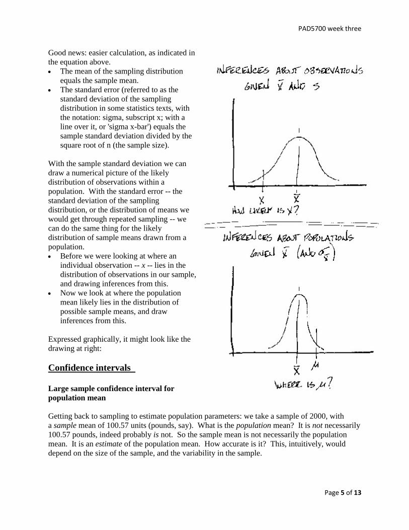
Before we were looking at where an

individual observation -- x -- lies in the

distribution of observations in our sample,

and drawing inferences from this.

Now we look at where the population

mean likely lies in the distribution of

possible sample means, and draw

inferences from this.

Expressed graphically, it might look like the

drawing at right:

Confidence intervals

Large sample confidence interval for

population mean

Getting back to sampling to estimate population parameters: we take a sample of 2000, with

a sample mean of 100.57 units (pounds, say). What is the population mean? It is not necessarily

100.57 pounds, indeed probably is not. So the sample mean is not necessarily the population

mean. It is an estimate of the population mean. How accurate is it? This, intuitively, would

depend on the size of the sample, and the variability in the sample.

PAD5700 week three

Page 6 of 13

The effect of sample size on accuracy of a population estimate should be relatively easy to get.

If you catch a fish which weighs five pounds, you have little information with which to conclude

that the mean population weight of this type of fish is five pounds. You might just have gotten

unlucky, picked a dwarf or something, or an Alex Rodriguez fish. But if you catch 10 of these

fish, and have a mean weight of five pounds, you can start to assume that the population mean

weight of these is about five, when caught from the place you caught them, at the time you

caught them, using the gear and bait you used, etc. (Note this latter proviso: in addition to

exercising caution regarding the accuracy of one's estimate of the population mean when one has

little data, one also has to be cautious concerning inferences drawn about populations not

relevant to the sampling operation -- or regarding the 'external validity' of the study.)

Getting back to our population estimate: one can especially be a bit more confident about an

estimate of a population mean given a sample of ten fish if the sample is fairly narrowly grouped

around five pounds. At a sample of 500 fish, you become even more confident that the

population mean weight is five pounds.

Still, ten different researchers drawing samples of 500 in an identical manner will get ten

different sample means, or ten different estimates of the population mean. 5 pounds, 5.1, 4.9, 4.9

again, 4.8, 5.2, 5.04, even the odd 4.4 or so. What, then, is the population mean? We don't

know, but can give an estimate within a 'confidence interval', which is the same thing as the

'margin of error' used in polling. We express the population mean in terms of an interval in

which we can have a certain confidence that the true population mean will lie. So we can't say

that the mean is 5.1 pounds, but we can (given details) say something like "we can be 95%

confident that the population mean lies within 0.3 pounds of 5.1; or between 4.8 and 5.4."

An example

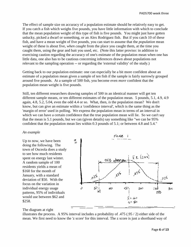
Up to now, we have been

doing the following. The

town of Osceola does a study

to see how much residents

spent on energy last winter.

A random sample of 100

residents yields a mean of

$160 for the month of

January, with a standard

deviation of $50. With the

focus on the variation in

individual energy usage

patterns, 95% of individuals

would use between $62 and

$258.

The diagram at right

illustrates the process. A 95% interval includes a probability of .475 (.95 / 2) either side of the

mean. We first need to know the 'z score' for this interval. The z score is just a shorthand way of

PAD5700 week three

Page 7 of 13

saying how many standard deviations a point is from the mean: a z score of two means

something is two standard deviations from the mean.

You will not have to do this, but the z score can be found in a z table (Appendix A, p. 324 in

Berman & Wang). To find the z score associated with a probability of 0.025 in the 'tails', or

either end of the distribution, we go to a probability of 0.475 (0.5 - 0.025) in the z table. The z

score for this is 1.96, so the interval within which we would expect 95% of the observations to

lie -- or the points at which we will identify the upper and lower tails of p(0.025) -- is 1.96

standard deviations either side of the mean.

This 95% confidence level is a commonly used one, the

margins of error in opinion polling are always expressed

in terms of a 95% confidence level, or 5% margin of

error. Other standard confidence levels (with associated z

score) can be found in Table 1.

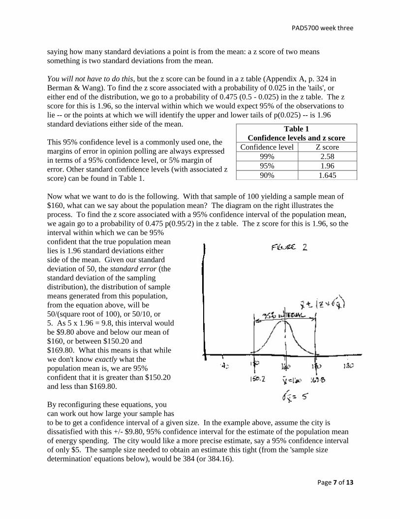
Now what we want to do is the following. With that sample of 100 yielding a sample mean of

$160, what can we say about the population mean? The diagram on the right illustrates the

process. To find the z score associated with a 95% confidence interval of the population mean,

we again go to a probability of 0.475 p(0.95/2) in the z table. The z score for this is 1.96, so the

interval within which we can be 95%

confident that the true population mean

lies is 1.96 standard deviations either

side of the mean. Given our standard

deviation of 50, the standard error (the

standard deviation of the sampling

distribution), the distribution of sample

means generated from this population,

from the equation above, will be

50/(square root of 100), or 50/10, or

5. As 5 x 1.96 = 9.8, this interval would

be $9.80 above and below our mean of

$160, or between $150.20 and

$169.80. What this means is that while

we don't know exactly what the

population mean is, we are 95%

confident that it is greater than $150.20

and less than $169.80.

By reconfiguring these equations, you

can work out how large your sample has

to be to get a confidence interval of a given size. In the example above, assume the city is

dissatisfied with this +/- $9.80, 95% confidence interval for the estimate of the population mean

of energy spending. The city would like a more precise estimate, say a 95% confidence interval

of only $5. The sample size needed to obtain an estimate this tight (from the 'sample size

determination' equations below), would be 384 (or 384.16).

Table 1

Confidence levels and z score

Confidence level Z score

99% 2.58

95% 1.96

90% 1.645

PAD5700 week three

Page 8 of 13

Clear as mud, huh!

SPSS -- tragically, SPSS generally won't calculate this for us. It will give us a mean, and a

standard error, with which we can calculate a confidence interval.

We've seen much of the above in our SPSS exercises so far. Open the income-NSBend file and

we can illustrate a lot of what we've been working on, though:

First, restrict the file only to South Bend. Do this by going to Data, Select Cases, ‘If

condition is satisfied’, click ‘If’, highlight ‘City’ and click the arrow to move it to the right,

then complete the equation: City = 1 (we coded North Bend = 0, South Bend = 1), Continue,

Okay.

Run descriptive statistics on the ten South Bend cases for income in 2000; including a mean,

standard deviation and standard error. These figures are 35.0, 5.9 and 1.9, respectively. The

SPSS output:

Table 2

Descriptive Statistics

N Mean Std. Deviation

Statistic Statistic Std. Error Statistic

2000 Income ($1000s) 10 35.0000 1.86190 5.88784

Valid N (listwise) 10

You can also derive these manually, just so that you can see what SPSS is doing:

o The mean of 35

(25 + 29 + 31 + 33 + 35 + 35 + 37 + 39 + 41 + 45)

10

= 35.0

o The standard deviation of 5.9

[(35-25)

2 + (35-29)

2 + (35-31)

2 + (35-33)

2 + (35-35)

2 + (35-35)

2 +

(35-37)2 + (35-39)

2 + (35-41)

2 + (35-45)

2] / (n-1)

so

[(10)2 + (6)

2 + (4)

2 + (2)

2 + (0)

2 + (0)

2 + (-2)

2 + (-4)

2 + (-6)

2 + (-10)

2] / (10-1)

so

100 + 36 + 16 + 4 + 0 + 0 + 4 + 16 + 36 + 100 / 9

so

312 / 9 = 34.67

square root of 34.67 = 5.9

o The standard error (or standard deviation of the sampling distribution)

5.9 / (square root of 10)

so

5.9 / 3.16 = 1.87

PAD5700 week three

Page 9 of 13

Given our data, a confidence interval estimate of the mean 2000 income for South Bend would

be:

95% C.I. =

95% C.I. = 30 +/- 1.96 x 1.7

95% C.I. = 30 +/- 3.65

or: you can be 95% confident that the population mean lies between 26.35 and 33.65.

Large sample hypothesis tests The general idea in hypothesis testing is to test the reliability of the status quo. In English (or

perhaps Statslish, as the jargon is inevitable), we draw a sample and obtain a sample mean from

this. It differs from what we expected, by which we mean what we thought the value should

have been, based on past experience, for the phenomenon in question. What can we infer from

this, though? Does it differ enough that it suggests that our status quo assumption is now

defunct? Or could our sample mean just have resulted from the randomness associated with

sampling?

McClave and Sincich present the elements of an hypothesis test, which I'll reproduce, modified

below. This is what Berman & Wang present in pages 174-7, though not quite as completely as

McClave & Sincich. Also, this goes through the process if you were doing it longhand. We will

mostly use SPSS, though, so I present the longhand method just in the hopes that the SPSS

output will make more sense. I also drop the ‘critical value’ part, and instead suggest reporting

the statistical significance of the test, for reasons that will be explained.

Elements of a Test of Hypothesis

1. Null hypothesis (H0): A theory about the values of one or more population parameters. The

theory generally represents the status quo, which we accept until it is proven false.

2. Alternative hypothesis (Ha): A theory that contradicts the null hypothesis. The theory

generally represents that which we will accept only when sufficient evidence exists to

establish its truth.

3. Assumptions: Clear statement(s) of any assumptions made about the population(s) being

sampled.

4. Experiment and calculation of test statistic and probability value: Performance of the

sampling experiment and determination of the numerical value of the test statistic.

5. Conclusion: If the numerical value of the test statistic is enough that you are comfortable

rejecting the null hypothesis, do so.

Source: McClave and Sincich, p. 282.

Remember that when rejecting the null hypothesis (the status quo assumption), you should be

careful about what you say about the population mean. When rejecting the null hypothesis, our

old, status quo assumption has been shown to be incorrect. However, we cannot now assume

that our sample mean is the population mean. We can only go back to our confidence intervals,

and provide an estimate of what our sample mean indicates the population mean is. The logic

here is that the null hypothesis, status quo population mean was tried and true, having been

determined some time ago and continually validated through subsequent observation. On

rejecting this, we need to do much more research before we can offer a new population mean, in

any event a single sample does not provide enough information on this.

PAD5700 week three

Page 10 of 13

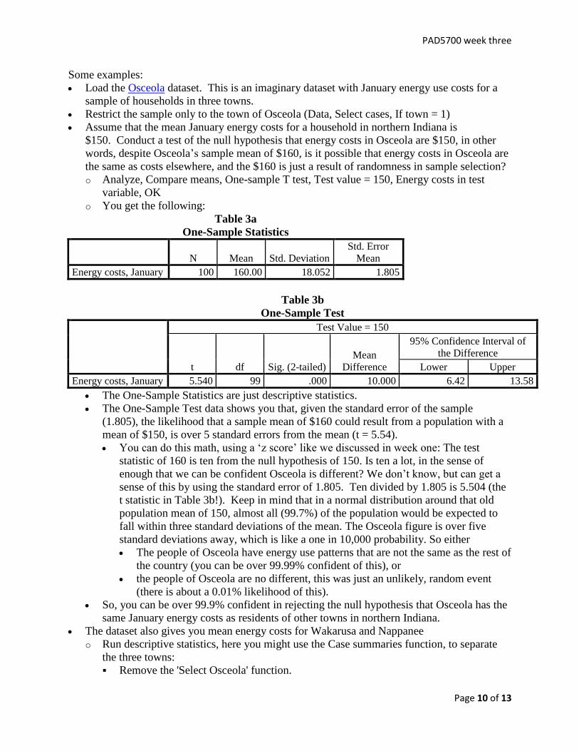
Some examples:

Load the Osceola dataset. This is an imaginary dataset with January energy use costs for a

sample of households in three towns.

Restrict the sample only to the town of Osceola (Data, Select cases, If town = 1)

Assume that the mean January energy costs for a household in northern Indiana is

$150. Conduct a test of the null hypothesis that energy costs in Osceola are $150, in other

words, despite Osceola’s sample mean of $160, is it possible that energy costs in Osceola are

the same as costs elsewhere, and the $160 is just a result of randomness in sample selection?

o Analyze, Compare means, One-sample T test, Test value = 150, Energy costs in test

variable, OK

o You get the following:

Table 3a

One-Sample Statistics

N Mean Std. Deviation

Std. Error

Mean

Energy costs, January 100 160.00 18.052 1.805

Table 3b

One-Sample Test

Test Value = 150

t df Sig. (2-tailed)

Mean

Difference

95% Confidence Interval of

the Difference

Lower Upper

Energy costs, January 5.540 99 .000 10.000 6.42 13.58

The One-Sample Statistics are just descriptive statistics.

The One-Sample Test data shows you that, given the standard error of the sample

(1.805), the likelihood that a sample mean of $160 could result from a population with a

mean of $150, is over 5 standard errors from the mean (t = 5.54).

You can do this math, using a ‘z score’ like we discussed in week one: The test

statistic of 160 is ten from the null hypothesis of 150. Is ten a lot, in the sense of

enough that we can be confident Osceola is different? We don’t know, but can get a

sense of this by using the standard error of 1.805. Ten divided by 1.805 is 5.504 (the

t statistic in Table 3b!). Keep in mind that in a normal distribution around that old

population mean of 150, almost all (99.7%) of the population would be expected to

fall within three standard deviations of the mean. The Osceola figure is over five

standard deviations away, which is like a one in 10,000 probability. So either

The people of Osceola have energy use patterns that are not the same as the rest of

the country (you can be over 99.99% confident of this), or

the people of Osceola are no different, this was just an unlikely, random event

(there is about a 0.01% likelihood of this).

So, you can be over 99.9% confident in rejecting the null hypothesis that Osceola has the

same January energy costs as residents of other towns in northern Indiana.

The dataset also gives you mean energy costs for Wakarusa and Nappanee

o Run descriptive statistics, here you might use the Case summaries function, to separate

the three towns:

Remove the 'Select Osceola' function.

PAD5700 week three

Page 11 of 13

Analyze, Reports, Case Summaries.

Variables = Energy costs; Group Variable = Town name.

Uncheck the Display Cases

Under Statistics ask for a whatever you want. Continue, Okay.

You should get this:

Table 4a

Case Summaries Energy costs, January

Town name Mean Median Minimum Maximum

Std. Error of

Mean Std. Deviation

Osceola 160.00 161.00 121 201 1.805 18.052

Wakarusa 150.00 153.00 120 178 2.600 16.444

Nappanee 158.90 158.50 120 196 3.031 19.171

Total 157.53 159.00 120 201 1.366 18.323

Now do an hypothesis test to see if energy costs differ between Osceola and Wakarusa.

o Analyze, Compare means, Independent-Samples T test, Test variable = Energy costs,

Town = Grouping variable, Define groups, Group 1 = 1 (Osceola), Group 2 = 2

(Wakarusa)

o You should get the following (I’ve reformatted to make it fit, especially getting rid of the

95% Confidence Interval of the Difference):

Table 5

Independent Samples Test

Levene's Test for

Equality of Variances t-test for Equality of Means

F Sig. t df

Sig. (2-

tailed)

Mean

Difference

Std. Error

Difference

Energy

costs,

January

Equal variances assumed .035 .852 3.035 138 .003 10.000 3.295

3.165 Equal variances not assumed

3.159 78.479 .002 10.000

The first table shows the two means: $160 for Osceola, $150 for Wakarusa. I’ll omit it

(we’ve got it above)

The second shows the likelihood that you would get different means for two samples of

these sizes (n = 100 for Osceola; n = 40 for Wakarusa). This is reflected in the Sig. (2-

tailed) figures of .002 or .003.

Which of these you choose to use isn't terribly important (it depends on whether you

think the variances between Osceola and Wakarusa are the same, which the Levene's Test

for Equality of Variances suggests is not the case), but what this tells you is that the

likelihood that you would randomly get means of $160 and $150 for these two samples, if

they came from the same population (and so should have the same mean), is .002, or very

unlikely. Given this, you can reject the null hypothesis that they come from the same

population. Instead, they differ.

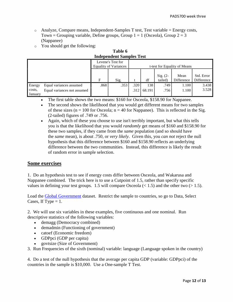
Do an hypothesis test to see if energy costs differ between Osceola and Nappanee.

PAD5700 week three

Page 12 of 13

o Analyze, Compare means, Independent-Samples T test, Test variable = Energy costs,

Town = Grouping variable, Define groups, Group 1 = 1 (Osceola), Group 2 = 3

(Nappanee)

o You should get the following:

Table 6

Independent Samples Test

Levene's Test for

Equality of Variances t-test for Equality of Means

F Sig. t df

Sig. (2-

tailed)

Mean

Difference

Std. Error

Difference

Energy

costs,

January

Equal variances assumed .868 .353 .320 138 .749 1.100 3.438

3.528 Equal variances not assumed

.312 68.191 .756 1.100

The first table shows the two means: $160 for Osceola, $158.90 for Nappanee.

The second shows the likelihood that you would get different means for two samples

of these sizes (n = 100 for Osceola; n = 40 for Nappanee). This is reflected in the Sig.

(2-tailed) figures of .749 or .756.

Again, which of these you choose to use isn't terribly important, but what this tells

you is that the likelihood that you would randomly get means of $160 and $158.90 for

these two samples, if they came from the same population (and so should have

the same mean), is about .750, or very likely. Given this, you can not reject the null

hypothesis that this difference between $160 and $158.90 reflects an underlying

difference between the two communities. Instead, this difference is likely the result

of random error in sample selection.

Some exercises

1. Do an hypothesis test to see if energy costs differ between Osceola, and Wakarusa and

Nappanee combined. The trick here is to use a Cutpoint of 1.5, rather than specify specific

values in defining your test groups. 1.5 will compare Osceola (< 1.5) and the other two (> 1.5).

Load the Global Government dataset. Restrict the sample to countries, so go to Data, Select

Cases, If Type = 1.

2. We will use six variables in these examples, five continuous and one nominal. Run

descriptive statistics of the following variables:

demagg (Democracy combined)

demadmin (Functioning of government)

catoef (Economic freedom)

GDPpci (GDP per capita)

govtsize (Size of Government)

3. Run Frequencies of the sixth (nominal) variable: language (Language spoken in the country)

4. Do a test of the null hypothesis that the average per capita GDP (variable: GDPpci) of the

countries in the sample is $10,000. Use a One-sample T Test.

PAD5700 week three

Page 13 of 13

5. Many folks fear that the US has slowly become more and more socialistic, like the rest of the

world, over the past couple of decades. The US score on the CATO Institute's Economic

Freedom (catoef) indicator is 8.1. Test to see if this is in line with the global norm. Again, use a

One-sample T Test.

6. Do a test of the null hypothesis that English and Spanish speaking countries do not differ in

terms of income. This would require an Independent-Samples T Test.

7. Do a similar test to see if rich countries have more effective government administrations

(demadmin) than poor ones. Do an Independent-Samples T Test, using $10,000 as a cut point.

8. Do a correlation to see if wealth (GDPpci) and administration (demadmin) are related.

9. Finally, it is widely argued that more government will lead to less democracy. Do a

correlation between Size of Government (govtsize) and Democracy (demagg).

*

References: Gold, Michael and G.G. Candler (2006). "The MPA Program in small markets: an exploratory

analysis." Journal of Public Affairs Education 12(1), pp. 49-62, 2006. Available online.

McClave, James and Terry Sincich (2003). A First Course in Statistics. Upper Saddle River,

NJ: Prentice Hall.