Multi-modal Semantic Indexing for Image Retrieval

Thesis submitted in partial fulfillment

of the requirements for the degree of

Master of Science (by Research)

in

Computer Science

by

P. L. Chandrika

200707009chandrika@research.iiit.ac.in

International Institute of Information Technology

Hyderabad, INDIA

December 2013

INTERNATIONAL INSTITUTE OF INFORMATION TECHNOLOGY

Hyderabad, India

CERTIFICATE

It is certified that the work contained in this thesis, titled “Multi modal Semantic Indexing for Image

Retrieval” by Miss. P. L. Chandrika, has been carried out under our supervision and is not submitted

elsewhere for a degree.

Date Prof. C. V. Jawahar,

Professor,

IIIT, Hyderabad

Copyright c⃝ P. L .Chandrika, 2013

All Rights Reserved

To CVIT, IIIT Hyderabad the place which taught me ,

what an image is and what information can be derived from it.

To my Family and Friends.

Acknowledgements

I am grateful to my advisor Dr. C V Jawahar for introducing me to research and believing that I could

do good research. Through the three years that I have spent on my thesis, i appreciate his patience for

bearing me through all the missed deadlines and naively written reports. It has been my pleasure to

actively collaborate and work with Suman Karthik, Sreekanth and Mihir. Further, I would like to thank

my friends, colleagues and fellow CVIT students, especially Suhail, Rakesh, Chetan, Maneesh, Karthika

and Jinesh. The effort Satya and Phani put into managing CVIT activities have been a major help . I

would also like to thank my IIIT friends especially Sri Lakshmi, Padmini and Jyothish for helping

me through out my stay in IIIT. Finally, I would like to thank the almighty, my parents, my relatives,

all those from CVIT and others who at some point or the other have helped me with their invaluable

suggestions and feedback. It goes without saying that Center for Visual Information Technology (CVIT)

as a research center has been pivotal in this thesis, both as a source of intellectual resources as well as

financial funding.

Abstract

Many image retrieval schemes generally rely only on a single mode, (either low level visual fea-

tures or embedded text) for searching in multimedia databases. In text based approach, the annotated

text is used for indexing and retrieval of images. Though they are very powerful in matching the context

of the images but the cost of annotation is very high and the whole process suffers from the subjectivity

of descriptors.

In content based approach, the indexing and retrieval of images is based on the visual content

of the image such as color, texture, shape, etc. While these methods are robust and effective they are

still bottlenecked by semantic gap. That is, there is a significant gap between the high-level concepts

(which human perceives) and the low-level features (which are used in describing images). Many ap-

proaches(such as semantic analysis) have been proposed to bridge this semantic gap between numerical

image features and richness of human semantics

Semantic analysis techniques were first introduced in text retrieval, where a document collection

can be viewed as an unsupervised clustering of the constituent words and documents around hidden or

latent concepts. Latent Semantic Indexing (LSI), probabilistic Latent Semantic Analysis (pLSA), Latent

Dirichlet Analysis (LDA) are the popular techniques in this direction. With the introduction of bag of

words (BoW) methods in computer vision, semantic analysis schemes became popular for tasks like

scene classification, segmentation and content based image retrieval. This has shown to improve the

performance of visual bag of words in image retrieval. Most of these methods rely only on text or image

content.

Many popular image collections (eg. those emerging over Internet) have associated tags, often for

human consumption. A natural extension is to combine information from multiple modes for enhancing

effectiveness in retrieval.

The enhancement in performance of semantic indexing techniques heavily depends on the right

choice of number of semantic concepts. However, all of them require complex mathematical compu-

tations involving large matrices. This makes it difficult to use it for continuously evolving data, where

repeated semantic indexing (after addition of every new image) is prohibitive. In this thesis we intro-

duce and extend, a bipartite graph model (BGM) for image retrieval. BGM is a scalable datastructure

that aids semantic indexing in an efficient manner. It can also be incrementally updated. BGM uses

tf-idf values for building a semantic bipartite graph. We also introduce a graph partitioning algorithm

that works on the BGM to retrieve semantically relevant images from a database. We demonstrate the

properties as well as performance of our semantic indexing scheme through a series of experiments.

Then , we propose two techniques: Multi-modal Latent Semantic Indexing (MMLSI) and Multi-

Modal Probabilistic Latent Semantic Analysis (MMpLSA). These methods are obtained by directly

extending their traditional single mode counter parts. Both these methods incorporate visual features and

tags by generating simultaneous semantic contexts. The experimental results demonstrate an improved

accuracy over other single and multi-modal methods.

We also propose, a tri-partite graph based representation of the multi model data for image re-

trieval tasks. Our representation is ideally suited for dynamically changing or evolving datasets, where

repeated semantic indexing is practically impossible. We employ a graph partitioning algorithm for re-

trieving semantically relevant images from the database of images represented using the tripartite graph.

Being ”just in time semantic indexing”, our method is computationally light and less resource intensive.

Experimental results show that the data structure used is scalable. We also show that the performance of

our method is comparable with other multi model approaches, with significantly lower computational

and resources requirements

ii

Contents

1 Introduction 2

1.1 Introduction . . . . . . . . . . . . . . . . . . . . . . . . . . . . . . . . . . . . . . . 2

1.1.1 Multimedia and Multimodal Data . . . . . . . . . . . . . . . . . . . . . . . . 2

1.1.2 Traditional Image Retrieval . . . . . . . . . . . . . . . . . . . . . . . . . . . 3

1.1.3 Semantics in Image Retrieval . . . . . . . . . . . . . . . . . . . . . . . . . . 4

1.1.4 Semantics and Text Retrieval . . . . . . . . . . . . . . . . . . . . . . . . . . . 5

1.1.5 Semantics and Visual bag of word(bow) modal . . . . . . . . . . . . . . . . . 7

1.1.6 Multimodal Data . . . . . . . . . . . . . . . . . . . . . . . . . . . . . . . . . 9

1.2 Problem Statement and Contributions . . . . . . . . . . . . . . . . . . . . . . . . . . 9

1.3 Organization of the Thesis . . . . . . . . . . . . . . . . . . . . . . . . . . . . . . . . 11

2 Background on Semantic Indexing 13

2.1 Content Base Image Retrieval . . . . . . . . . . . . . . . . . . . . . . . . . . . . . . 13

2.2 Semantic analysis . . . . . . . . . . . . . . . . . . . . . . . . . . . . . . . . . . . . . 15

2.2.1 Latent Semantic Analysis(LSA) . . . . . . . . . . . . . . . . . . . . . . . . . 15

2.2.2 Probabilistic Latent Semantic Analysis (pLSA) . . . . . . . . . . . . . . . . . 17

2.2.3 Incremental Probabilistic Latent Semantic Analysis (IpLSA) . . . . . . . . . . 19

2.3 Graph Traversal Methods . . . . . . . . . . . . . . . . . . . . . . . . . . . . . . . . . 20

2.4 Multimodal Retrieval . . . . . . . . . . . . . . . . . . . . . . . . . . . . . . . . . . . 22

3 Bipartite Graph Model(BGM) 25

3.1 Problem Setting . . . . . . . . . . . . . . . . . . . . . . . . . . . . . . . . . . . . . 25

3.2 BGM . . . . . . . . . . . . . . . . . . . . . . . . . . . . . . . . . . . . . . . . . . . 26

3.2.1 A Graph Partition Scheme . . . . . . . . . . . . . . . . . . . . . . . . . . . . 27

i

3.3 Results and Discussion . . . . . . . . . . . . . . . . . . . . . . . . . . . . . . . . . . 28

3.4 Summary . . . . . . . . . . . . . . . . . . . . . . . . . . . . . . . . . . . . . . . . . 32

4 Multi Modal Semantic Indexing 33

4.1 Problem Setting . . . . . . . . . . . . . . . . . . . . . . . . . . . . . . . . . . . . . . 33

4.2 Tensor Concepts . . . . . . . . . . . . . . . . . . . . . . . . . . . . . . . . . . . . . . 33

4.3 Multi Modal Latent Semantic Indexing . . . . . . . . . . . . . . . . . . . . . . . . . . 35

4.4 Semantic Indexing By Multi-Modal pLSA . . . . . . . . . . . . . . . . . . . . . . . . 36

4.5 Indexing and Retrieval . . . . . . . . . . . . . . . . . . . . . . . . . . . . . . . . . . 39

4.5.1 Feature Extraction . . . . . . . . . . . . . . . . . . . . . . . . . . . . . . . . 40

4.5.2 Image Retrieval Framework . . . . . . . . . . . . . . . . . . . . . . . . . . . 40

4.6 Results and Discussions . . . . . . . . . . . . . . . . . . . . . . . . . . . . . . . . . 43

4.6.1 Data Sets . . . . . . . . . . . . . . . . . . . . . . . . . . . . . . . . . . . . . 43

4.6.2 Experimental Results . . . . . . . . . . . . . . . . . . . . . . . . . . . . . . . 44

4.7 Summary . . . . . . . . . . . . . . . . . . . . . . . . . . . . . . . . . . . . . . . . . 46

5 Tripartite Graph Modal 47

5.1 Problem Setting . . . . . . . . . . . . . . . . . . . . . . . . . . . . . . . . . . . . . . 47

5.2 Tripartite Graph Representation and Retrieval . . . . . . . . . . . . . . . . . . . . . . 47

5.2.1 Learning Edge Weights . . . . . . . . . . . . . . . . . . . . . . . . . . . . . . 49

5.2.2 Offline Indexing . . . . . . . . . . . . . . . . . . . . . . . . . . . . . . . . . 50

5.3 Results and Discussions . . . . . . . . . . . . . . . . . . . . . . . . . . . . . . . . . . 51

5.3.1 BGM and offline BGM . . . . . . . . . . . . . . . . . . . . . . . . . . . . . . 51

5.3.2 Multimodal Retrieval . . . . . . . . . . . . . . . . . . . . . . . . . . . . . . . 52

6 Conclusion 55

6.1 Future Work . . . . . . . . . . . . . . . . . . . . . . . . . . . . . . . . . . . . . . . . 56

Related Publications 57

ii

List of Figures

1.1 Existing Text based image retrieval systems(left to right, top to bottom) Google, Picasa,

Bing, flickr, Rediff Image Search and Facebook. . . . . . . . . . . . . . . . . . . . . 4

1.2 The image shows the semantic gap, here the color based features are unable to differen-

tiate between these images representing different concepts(here objects). . . . . . . . 6

1.3 The image (a) is an example from dataset UW [1] with the annotation (b) is an example

from dataset Multi-label with the annotations [2], and (c) is an example from dataset

IAPR with small description of the image [3]. . . . . . . . . . . . . . . . . . . . . . . 10

2.1 The above diagram shows the visual vocabulary generation using bag of words model

in computer vision. Here the images are sampled and image patches are extracted using

local detectors. These patches are further encoded into a feature vector using local de-

scriptors. Then clustering method(k-means) is used to quantized the feature vector space

to create visual words. Finally the image is represented as a histogram of visual words.

The important thing to note is that the spatial consistency among the words/patches is

not maintained in the BoW model. . . . . . . . . . . . . . . . . . . . . . . . . . . . . 15

2.2 The figure shows a Term-Document Matrix where the columns represents the terms in

the document, the rows represent the image and the each value in the matrix gives the

frequency of the occurrence of certain visual word in each image. . . . . . . . . . . . 16

2.3 Latent Semantic Indexing Model . . . . . . . . . . . . . . . . . . . . . . . . . . . . . 17

2.4 Standard plsa Model . . . . . . . . . . . . . . . . . . . . . . . . . . . . . . . . . . . 18

3.1 An Example of Bipartite graph. The two sets U and V may be thought of as a coloring

of the graph with two colors: if we color all nodes in U blue, and all nodes in V green,

each edge has endpoints of differing colors, as is required in the graph coloring problem. 26

iii

3.2 Graphical representation of Bipartite Graph Model. The image in the database is repre-

sented as a collection of visual words. The edges connect the visual words to the images

in which they are present. . . . . . . . . . . . . . . . . . . . . . . . . . . . . . . . . . 29

3.3 The result of retrieval on Zurich building data for simple indexing and BGM, first image

is query image. . . . . . . . . . . . . . . . . . . . . . . . . . . . . . . . . . . . . . . 30

3.4 The retrieval performance of PLSA varying the number of Concepts. . . . . . . . . . . 31

4.1 The figure shows visual word - text word - document tensor and its decomposition . . . 36

4.2 Graphical representation of Multi Modal pLSA . . . . . . . . . . . . . . . . . . . . . 37

4.3 Over view of the Process . . . . . . . . . . . . . . . . . . . . . . . . . . . . . . . . . 40

4.4 The first image of each row is the query, other two are the retrieved results. Each row

corresponds to the IAPR, UW and Multi-label datasets respectively . . . . . . . . . . . 43

5.1 Tri-partite Graph Representation of dataset, twi are text words, vwi are visual words and

di are the images . . . . . . . . . . . . . . . . . . . . . . . . . . . . . . . . . . . . . 49

5.2 The first image is the query, the rest of the images in the first column are the visual

results, the images in the second column were obtained when text query “Cyclist in

Australia”was given. Last column comprises of multimodal results of TGM-learning. . 54

iv

List of Tables

3.1 Mean Average Precision for both BGM, pLSA and IpLSA for the holiday dataset, along

with time taken to perform semantic indexing and memory space used during indexing. 31

4.1 Comparing Multi Modal LSI with different forms of LSI for all the datasets in mAP. . 44

4.2 Comparing Multi Modal PLSA with different forms of PLSA for all the datasets in mAP. 44

5.1 Mean Average Precision for both BGM online and offline for the holiday dataset, along

with time taken to perform semantic indexing and memory space used during indexing. 51

5.2 Comparing TGM with Multi Modal LSI and Multi Modal pLSA for different the datasets 52

5.3 Mean Average Precision for both TGM, MMLSI, MMpLSA and mm-pLSA for the UW

dataset, along with time taken to perform semantic indexing and memory space used

during indexing. . . . . . . . . . . . . . . . . . . . . . . . . . . . . . . . . . . . . . . 53

1

Chapter 1

Introduction

1.1 Introduction

Capturing human experiences in record, and sharing them with others has been an important activity

since the beginning of the camera era. In the film based imaging era, the data could not be easily copied

and stored. Hence data sharing was limited to direct access to limited copies. Invention of the digital

camera has given the common man the privilege to capture his world, and conveniently share them with

others. The data storage and copying has hence become a trivial and non expensive process. Easily

available storage devices and a huge market for online repositories has created a spurt in web based data

hosting services. The data can thus be easily stored and shared on third party hardware and accessed

through the Internet. With the popularity of large multimedia repositories over Internet increasing, need

for effective access is on the rise. Low-cost storage and easy web hosting has changed a common man

from a passive consumer of multimedia in the past to a current-day active producer. Such user generated

data is easily available for other users to access.

1.1.1 Multimedia and Multimodal Data

Multimedia data may ideally consists of text, image, graphics, animations, audio and video converted

from different formats into digital media. In this context, a multimedia database refers to a data col-

lection in which multiple modalities exist. In this thesis, we focus on databases of text and imagery.

Sharing of such multimedia data has moved from a potential area for revenues, to an active revenue

generator for many corporates. Thus, multimedia sharing industry has matured over the years. The

2

advances is not just in storage, but efficient indexing and retrieval of such multimedia databases, has

thrown of interesting problems, methods and results. Such processing of stored multimedia data is spe-

cific to type of its content. Broadcast news videos is an example of multimedia data which contains

video, audio and overlaid text. Summarizing such videos is important for many applications such as

archiving video news programs. Broadcast news video summarization requires details of story or topic

boundaries in the video as well as understanding the semantics of the linguistic and visual content as-

sociated with the news. An other important modality in multimedia data is Images. Indexing image

data poses more challenge than compared to text data. This is due to the lack of understanding of the

image context, specially in the absence of user given text tags. The universe of the context of the image

data is undefined. One can today generate volumes of images with visual content as diverse as family

get-together and national park visits.

One important problem that arises is the requirement to efficiently index data. Today, image data

exists with extremely diverse visual and semantic content, spanning geographically disparate locations,

and is rapidly growing in size. All these factors have created innumerable possibilities and hence con-

siderations for real-world image search system designers. Searching and indexing in such databases

creates interesting challenges for the indexing and retrieval community. Once an image is indexed, the

second aspect is efficient retrieval. This thesis addresses some of the issues associated with indexing

and retrieval of multimedia data, specially for databases with text tags and images.

1.1.2 Traditional Image Retrieval

Image retrieval is the process of browsing, searching and accessing images from a large database of

digital images. Most of the existing image retrieval systems use either the surrounding text or low-

level features of the images to search at content-level. In text based approach, images are annotated by

text descriptors which are then indexed efficiently to achieve real-time retrieval [4–6]. In this scenario,

cost of accurate annotation is very high and the whole process suffers from subjectivity of descriptors.

Generating efficient indexes from not just user generated tags, but also from the image content (say

features extracted from images) is an interesting challenge. The problem is non-trivial because image

databases contain images from a large variety of sources and content. To address this problem, content

based image retrieval (CBIR) was introduced. CBIR tries to index data based on the visual content of

the image. CBIR currently utilizes naive features, such that images are indexed by their visual content

such as color, texture, shape, spatial relationships etc [7]. The research in this area is well established.

3

A detailed discussion is given in Chapter 2.

It is to be noted that CBIR is based on directly analyzable low level features, which may not

help understand the context of the image, but would be rather interested in finding a statistical means

of retrieving images based on low level features. Such a method can be criticized for lacking focus

on generating an understanding of the image. Also is contrary to the way humans analyze images.

Humans tend to interpret images and their similarity, based on high-level features(concepts). Where as a

machine understandable terminology would be key words(frequency of key words) and text descriptors.

A fair intermediatory step to bridge the gap between human interpretation is to use keywords and text

descriptors. Using these along with low level image descriptors, allows to form a stronger understanding

of the context of the image. While the features automatically extracted using computer vision techniques

are mostly low-level features, they provide perceptual information of images which is useful in indexing.

Hence totally neglecting the image features is not a feasible option. Commercial systems basically relied

only on textual tags, off late they have started using visual features as a complementary information. The

Figure 1.1 shows examples of the publicly existing image retrieval systems.

Figure 1.1: Existing Text based image retrieval systems(left to right, top to bottom) Google, Picasa,

Bing, flickr, Rediff Image Search and Facebook.

1.1.3 Semantics in Image Retrieval

Semantic Gap: In Image Retrieval, low-level visual features directly relate to the perceptual aspect of

the image content. These features are usually easy to extract and represent. As well as fairly convenient

4

to design similarity measures by using the statistical properties of these features. High-level concepts,

however, are not extracted directly from visual contents, but they represent the relatively more important

meanings of objects and scenes in the images that are perceived by human beings. These conceptual

aspects are more closely related to user’s preferences and subjectivity. In general, there is no simple

direct link between a high-level concepts and the low-level features. The difference between the two

modes of information is known as the semantic gap [8].

Here concepts pertains to an abstract or general idea inferred or derived from the visual informa-

tion. There is incomplete understanding of the human context recognition mechanism and absence of

a polynomial time algorithm for the same. From an algorithmic perspective, this has lead to efforts

to understand the gap between user and machine. This area of research, though extensive and cross

disciplinary, has found limited success in bridging the gap in between the user and machine. From an

image retrieval perspective, this brings up the question of relation between the image features and image

concepts. Example of a feature could be ”red in color” while the relevant concept could be ”delicious

fruit”, as in Figure 1.3 we can see the semantic gap between the color features and concepts(objects).

As explained above, the semantic gap is a complex problem, which cannot be easily solved. Mul-

tiple methods which can perform the task in practical number of machine clock cycles have been de-

veloped. A detailed list of methods published earlier can be found in the survey paper [9]. A common

feature among these solutions is the category attached to these solutions, namely semantic analysis. As

the name suggests, it is an attempt to understand the semantics of the given data.

1.1.4 Semantics and Text Retrieval

Text retrieval is majorally categorized into two technologies and research: statistical and semantic.

Statistical approaches break documents and queries into terms. Most commonly, the terms are words that

occur in a given query or collection of documents. These terms are counted and measured statistically.

A numeric weight can be assigned to each term or word in a given document, representing an estimate

(usually but not necessarily statistical) of the usefulness of the given word as a descriptor of the given

document, i.e., an estimate of its usefulness for distinguishing the given document from other documents

in the same collection. It should be stressed that a given word may receive a different weight in each

document in which it occurs, a word may be a better descriptor of one document than of another. This

representation of documents is mainly referred to as Bag of Words model(BoW). Often these words

are pre-processed such as stemming to extract the root word and elimination of common words that

5

Figure 1.2: The image shows the semantic gap, here the color based features are unable to differentiate

between these images representing different concepts(here objects).

have little power to discriminate relevant from non-relevant documents, e.g., ”the”, ”it”, etc. Boolean,

extended boolean, vector space, and probabilistic are examples of such statistical approaches. Some

techniques break documents and queries into n-grams, i.e., arbitrary strings of n consecutive characters.

Human beings find it amazingly easy to assess the relevance of a given document based on syntax

and semantics. They find statistical and probabilistic methods much more difficult, tedious and error

prone. But for automated systems, the situation is the reverse. They can perform statistical calculations

easily. Developing automated systems that can understand documents in the syntactic/semantic sense

is much more difficult. As a result, most of the text retrieval systems have been based on statistical

methods. Increasingly however, syntactic and semantic methods are being used to supplement statistical

methods. The reason is plain. Even the best statistical or probabilistic methods will miss some relevant

documents and retrieve irrelevant documents. The hope is that an appropriate combination of traditional

statistical/probabilistic methods and syntactic/semantic methods will perform better than the statistical

methods alone.

The essence of semantic analysis is in decomposing the original signal/representation according

to a generative process. The parameters associated with the generative process is learned from the

examples. This is often achieved by a factorization scheme [10] or an Expectation Maximization (EM)

6

based component extraction [11]. This learning process typically provides a new feature representation,

which is data dependent. Thus, it is also viewed as dimensionality reduction.

Understanding higher levels concepts based on mathematical modeling has found success in most

applications. Latent Semantic Indexing (LSI), probabilistic Latent Semantic Analysis (pLSA) [11],

Latent Dirichlet Analysis (LDA) [12] are the popular techniques in this direction. These methods assume

availability of documents with set of words in them. Each of these techniques use hidden concepts in

data which is utilized for indexing and retrieval purposes. An easy assumption is that the number of

concepts is equal to the number of unique words. The challenge here is to reduce the number of concepts

to a manageable number. Such that the retrieval performance is optimized. LSI does so by performing

an SVD decomposition of the term-document matrix. The number of singular values are truncated, so

as to hold only the relevant values. Further processing is done on the resulting truncated matrix. pLSA

is a probabilistic model of semantic analysis. It tries to find concepts which fit the data in a probabilistic

manner. The probabilities are found using an expectation maximization method. Both these methods

rely on what can be called as a Bag of Words model. Where the relative order of words in a document

are irrelevant. It can be easily found that such model has its own shortcomings. To overcome these, a

model where each document has a Dirichlet prior in the distribution of words was used. This method is

called as Latent Dirichlet Allocation (LDA). The method is similar to pLSA, and equivalent when the

Dirichlet prior is uniform.

1.1.5 Semantics and Visual bag of word(bow) modal

With the development of Internet, the size of online digital image collections is increasing rapidly. A

large variety of Imaging hardware(such as digital cameras) are available in the market for all kinds of

customers and prices, which are being embedded in lots of digital devices such as mobile phones, ipods

etc. Due to the increase in huge cheap storage devices, numerous web-services such as social networks,

blogs and specialized photo sharing sites have emerged. Where thousands of images are added every

minute. In many of these repositories, images get tagged or annotated by users. Such textual tags

remain the primary method for accessing/searching such image collections. Therefore the necessity for

efficient as well as effective retrieval methods for large scale dynamic image collections, is on the rise.

Semantic indexing schemes are applied for effective search in text as well as image databases [11, 13].

Even in a single domain of multimedia analysis, these techniques are popular in multimedia processing

for applications ranging from retrieval [14] to annotation [15]. The semantic analysis tries to model data

7

into classes of concepts. These concepts have a substantial abstraction from the underlying low level

data. Hence, the concepts generated are generic in nature. Since these techniques model the concept of

interest in a generic manner, they are shown to be superior to the direct feature based methods. They

are very effective, when the concept of interest is complex and the number of examples is limited. Thus

the basic mathematical models behind the text modeling and retrieval literature [10–12] were effectively

extended for vision tasks [16–18].

The concept of Bag of words was thus extended to vision tasks. Visual bag of words approach rep-

resents the image as a histogram of visual words. With the introduction of bag of words (BoW) methods

in computer vision, semantic analysis schemes became popular for tasks like scene classification and

segmentation [19, 20]. Matching problem is then modeled as the estimation of similarities between

given histograms (or probability distributions). With this modeling, it became possible to explain the

image in terms of a predefined vocabulary [21].

Semantic indexing in a dynamic image collection poses a considerable challenge. As new images

are constantly added to an image collection the semantic index is unable to accurately represent the

changing database. This necessitates updation of the semantic model and indexing it at regular intervals

which is time consuming and not scalable for large databases with millions of latent concepts. As the

number of images and associated concepts increases, these computations become expensive. To address

this problem methods were designed such as, Incremental pLSA. There are many other incremental vari-

ants of pLSA [22]. The performance of some of these methods both in terms of computation efficiency

and retrieval performance are quite good. Yet they do not effectively address the issue of updating the

number of global latent concepts as the database grows. In chapter 3 we explain a scalable semantic

indexing schemes for largescale, dynamic, image collections. That is, given a query, we want to re-

trieve the relevant images from a constantly changing database that could range in size from millions to

billions of images.

Image retrieval has matured a lot in the recent years. On one end of the spectrum, we see successful

laboratory prototypes to retrieve similar images from large image collections based on visual bag of

words (BoW) model [21, 23]. On the other end of the spectrum, we see commercial systems with

very rich user base sharing photographs, and enabling browsing based on manually attached textual

tags [4]. But the current retrieval systems use either text or visual features in isolation. However, in

many practical cases, information available is richer and consists of both these modalities. For example

web pages contains text, imagery and other forms of information. Thus, image retrieval systems need to

8

focus on exploiting the synergy between different modes in improving the retrieval efficiency. There is

now active interest in integrating text and visual content of images for building effective image retrieval

systems [15, 24–27]. Multimodal techniques have shown prospects in many tasks including image

retrieval, video search and summarization [15, 28, 29]. Romberg et al. [26] proposed a mm-pLSA,

with two separate leaf-pLSAs, and a single top level pLSA node merging the two leaf-pLSAs. Here,

they apply pLSA to each mode, i.e., visual features and textual words separately, and then concatenate

the derived topic vectors of each mode to learn another pLSA on top of that.

1.1.6 Multimodal Data

A multimedia database refers to a data collection in which there are multiple modalities of data. In this

database system, the data in different modalities are related to each other. For example, a web page

consisting of text, image, audio and video. By multimodal data analysis in a multimedia database it

is meant that the knowledge discovery to the multimedia database is initiated by a query that may also

consist of multiple modalities of data such as text and imagery. Here, we focus on a multimedia database

as an image database in which each image has a few textual words given as annotation. The Figure 1.3

shows examples of such databases. We address the problem of multimodal data such as image database

as the problem of retrieving similar data from the database.

Semantic analysis works well for single mode data, where data is represented in a single type. Such

as a text only database, or a image database. However, many of the emerging databases are multimodal

in nature. In many of the applications such as web, domain-archived image databases (in which there are

annotations to images), and even consumer photo collections have rich collateral information coexisting

with image data. In addition to the improved retrieval accuracy, another benefit for the multimodal

approaches is the added querying modalities. Users can query an image database either by image, or by

a collateral information modality (e.g., text), or by any combination. For example, the image collections

over Internet can be effectively searched with a combination of textual and image clues.

1.2 Problem Statement and Contributions

In this thesis, we demonstrate two techniques, Multi-modal Probabilistic Latent Semantic Analysis

(pLSA) and Multi-modal Latent Semantic Indexing (LSI). These methods incorporate both visual fea-

tures and tags by generating semantic contexts. In the next chapters,

9

Figure 1.3: The image (a) is an example from dataset UW [1] with the annotation (b) is an example

from dataset Multi-label with the annotations [2], and (c) is an example from dataset IAPR with small

description of the image [3].

• LSI is extended to Multi-modal LSI, with a tensorial representation and Higher Order SVD.

• pLSA is extended to Multi-modal pLSA by combining multiple modes into a single context, and

then using EM algorithm to fit the model parameters.

• Superiority of the proposed methods is demonstrated over standard data sets. We compare our

results with other methods.

Semantic indexing schemes proposed in the literature are primarily for a single mode data [19].

There are also attempts for extending them to multimodal data [14, 26, 30]. However, all of them re-

quire complex mathematical computations involving large matrices. This makes it difficult to use it for

continuously evolving data, where repeated semantic indexing (after addition of every new image) is

prohibitive. In the later part of this thesis, we propose a tripartite graph based approach for multi model

image retrieval for dynamically changing datasets. We represent the data as a graph, with simple proce-

dures for insertion. Given a query image, we employ a graph partitioning scheme for separating relevant

images from the irrelevant ones and thereby retrieving images from the database. This is an extension

of our work Bipartite Graph Model explained in chapter 3. The experimental results show that the data

10

structure used is scalable, and ideally suited for incremental computation. With a computationally effi-

cient technique, we report results on standard data set, where we show that our retrieval is as effective

as that of the best reported multimodal semantic indexing schemes.

Thus the contributions of thesis are :

1. LSI is extended to Multi-modal LSI, with a tensorial representation and Higher Order SVD.(

Chapter 4) .

2. pLSA is extended to Multi-modal pLSA by combining multiple modes into a single context, and

then using EM algorithm to fit the model parameters( Chapter 4).

3. A Tripartite Graph based representation of images(Chapter 5).

4. A graph partitioning algorithm(explained in Chapter 3) is refined for retrieving relevant images

from a tripartite graph model(Chapter5).

1.3 Organization of the Thesis

Chapter 2 gives the technical background for reading the thesis. This gives detailed explanation of

Latent Semantic Indexing (LSI) and probabilistic Latent Semantic Analysis(pLSA). This chapter also

presents the literature survey on Multi-modal Image Retrieval. Chapter 3 gives a detailed explanation of

Bipartite Graph Modal (BGM) which is a scalable datastructure that aids in on-line semantic indexing.

It can also be incrementally updated. BGM uses tf-idf values for building a semantic bipartite graph. We

also introduce a graph partitioning Algorithm that works on the BGM to retrieve semantically relevant

images from the database. We examine the properties of both BGM and Cash Flow algorithm through

a series of experiments. Finally, we demonstrate how they can be effectively implemented to build

large scale image retrieval systems in an incremental manner. In Chapter 4, we give a Multi-modal

extension to the two methods mentioned in Chapter 2 i.e., LSI and pLSA, where both text and visual

content are used to construct am effective image retrieval systems. The experimental results shows an

improvement over other single and multi-modal methods. In Chapter 5, We explain a tri-partite graph

based representation of the multi model data for image retrieval tasks. This representation is ideally

suited for dynamically changing or evolving datasets, where repeated semantic indexing is practically

impossible. We employ a graph partitioning algorithm for retrieving semantically relevant images from

the database of images represented using the tripartite graph. Being a just in time semantic indexing,

11

our method is computationally light and less resource intensive. Experimental results show that the data

structure used is scalable. We also show that the performance of our method is comparable with other

multi model approaches, with significantly lower computational and resources requirements. Finally the

conclusions of the thesis are given in Chapter 6.

12

Chapter 2

Background on Semantic Indexing

2.1 Content Base Image Retrieval

In a content based image retrieval system, the search is done by analyzing the content of the image

rather than keywords or tags associated with the image. Here the content refers to color, texture, shape

or any other information derived from the image. The method to capture the content of the image

is known as feature extraction. Then the extracted content from the image is described as a multi-

dimensional feature vector also know as descriptors. The features can be extracted globally or locally.

Some of the frequently used global features are color histogram, color moments, color sets gabor filters,

co-occurrence matrix, shape content etc [8]. For retrieval, when a query is given it is represented as a

feature vector by the system. The distance between the query feature vector and the feature vectors from

the database is computed using a distance measure [31] and ranked. Retrieval is often done by using

indexing scheme(such as R-Trees [32], X-Trees [33], S-Trees and variants of R-Trees and S-Trees [34])

for efficient retrieval. In IBMs QBIC system [35], retrieval is done by combination of colour, texture

or shape as well as by text keyword. Image queries can be formulated by selection from a palette, as

an example image, or by sketching. Retrieval uses an R*-tree index for efficiency. The VIR Image

Engine from Virage, Inc [36] supports modular development and is available as Oracle DB add-ons.

It is used to power the Photo Finder system from Alta Vista. A detailed description of existing CBIR

systems can be found in [7, 8, 37, 38]. Methods from the object recognition, object classification and

text retrieval communities have been adopted in CBIR systems. Mainly local detectors and descriptors

from the object classification community are used for better image modeling, retrieval methods and

13

document indexing(such as semantic indexing) are adapted from text retrieval community. First we give

a brief description of how local descriptor and bag of words(BOW) model (adapted from text retrieval

community) are used for representing image to improving performance of CBIR systems. Then we give

a detailed discussion of adapting semantic analysis in CBIR to bridge sematic gap.

Local descriptors: Local descriptors are used to encode image point or patch data from the interest

point or region detectors. The aim of local descriptors is to encode the image patch into a representation

that are highly distinctive, invariant to affine photometric changes, invariant to rotation and scaling. To

compute local descriptors first regions are detected within the image from which local descriptors are

calculated. For considering a region detector as a good region detector they have to meet some criteria

like they must be scale invariant, rotation invariant, robust to affine photometric changes, etc. These

include scale and affine invariant detectors, blob detectors, affine covariant detectors, DoG(Difference of

Gaussian), LoG(Laplacian of Gaussian), MSER, Harris Affine, Hessian Affine and many such detectors.

Some of the widely used descriptors include SIFT [39], PCA-SIFT [40], GLOH [41], SURF [42]. In

[41], a detailed study of the performance of many such detectors is discussed.

Bag of Words(BOW): A Bag of Words model is used in Natural Language Processing and In-

formation Retrieval [12, 43] where a document is represented as an unordered collection of words.

Recently bag of words model has been adapted to computer vision, especially for object categorization

and recognition [44]. To represent image in a BOW model, each image is treated as document and

words in the image known as visual words are determined. This is done in three steps: feature detection,

feature representation and codebook generation. In feature detection, several local patches or regions

are considered. For example in interest point detection, salient patched such as edges, corners and blobs

in an image are detected. These salient patches are considered more important that other patches. Harris

affine detector, Difference of Gaussian(DoG) are examples of such detectors. In feature representation,

these patches are represented/converted in a numerical vector known as feature descriptor. Generally a

good descriptor should be invariant to scale, rotation and affine. Finally, from theses feature descrip-

tors codebook or vocabulary is generated where each codeword represents several patches. This vector

quantization is mainly done by using a k-means clustering method. Thus, each image is represented as

a distinct set of visual words or visual word histogram. Figure 2.1 shows the BoW model representation

of images.

14

Figure 2.1: The above diagram shows the visual vocabulary generation using bag of words model in

computer vision. Here the images are sampled and image patches are extracted using local detec-

tors. These patches are further encoded into a feature vector using local descriptors. Then clustering

method(k-means) is used to quantized the feature vector space to create visual words. Finally the image

is represented as a histogram of visual words. The important thing to note is that the spatial consistency

among the words/patches is not maintained in the BoW model.

2.2 Semantic analysis

Semantic analysis techniques(like Latent Semantic Analysis (LSA), Probabilistic Latent Semantic Anal-

ysis (pLSA) [11] and Latent Dirichlet Allocation (LDA) [12]) were introduced to improve the retrieval

performance of content based image retrieval systems by reducing the semantic gap. Semantic analysis

can be viewed as an unsupervised clustering of the constituent words and documents or image around

hidden or latent concepts. A generative model is first learnt, and the learnt model is then used for map-

ping the problem from an input space to a novel feature space. It is believed that this new representation

is closer to the semantic description.

2.2.1 Latent Semantic Analysis(LSA)

LSA was first proposed by the text retrieval community for textual indexing [10]. Later Quelhas et

al. [45] demonstrated the efficiency of LSA for visual indexing. Here the vocabulary W = {w1, . . . , wNv}

15

Figure 2.2: The figure shows a Term-Document Matrix where the columns represents the terms in the

document, the rows represent the image and the each value in the matrix gives the frequency of the

occurrence of certain visual word in each image.

is formed by visual words obtained from the features extracted of images D = {di, . . . , dNd} to form

trem document matrix N (see Figure 2.2. Nv is the size of the vocabulary and Nd is the number of

images in the database. Here we use images and document interchangeable. The basic idea is to retrieve

documents based on their conceptual meaning using a term-documents matrix N (see Figure 2.3). The

elements of the matrix n(di, wj) specifies the number of times the word wj occurred in a document

di. Because of the semantic relationship in documents, it is argued that the term-document matrix N

is sparse and rank deficient, say of rank r. This term-document matrix is then decomposed into three

matrices by Singular Value Decomposition (SVD).

N = UΣV t (2.1)

where Σ ∈ Rm×n is a diagonal matrix with nonnegative diagonal elements called the singular val-

ues(eigen values), U ∈ Rm×m and V ∈ Rn×n are orthogonal matrices. The columns of matrices U

and V are called the left singular vectors(left eigen vectors) and the right singular vectors(right eigen

vectors)respectively. The decomposition can be computed so that the singular values are sorted by de-

creasing order. The k top largest eigenvalue values form the decomposed matrices are selected to form

a reduced matrix Nk,where k < r is the dimensionality of the latent space see Figure 2.3. Original data

16

Algorithm 1 LSI for Image Retrieval

1: INPUT: N is n × m term document matrix, q the query vector, k compute k largest eigenvalues

and eigenvectors(k¡n).

2: Decompose the matrix A using SVD and select the first k eigen values.

N = UΣV T

3: Compute the co-ordinates of the query vector.

qc = q′ × U × inv(Σ)

4: Calculate the similarity coefficient between the images V and the query vector qc.

is then mapped to this reduced dimension with a linear transformation. The general claim is that the

similarity between the documents or between documents and quires is more reliably estimated in the

reduced latent space representation than in the original representation.

Figure 2.3: Latent Semantic Indexing Model

2.2.2 Probabilistic Latent Semantic Analysis (pLSA)

pLSA is a generative model of the data with strong statistical foundation, where each document is repre-

sented by its word frequency. And the similarity between the documents is compared in a semantic space

which is more reliable than original representation. The pLSA was originally proposed by T.Hofmann

in the context of text document retrieval [11], where each document is represented as a bag-of-words

representation. It has also been applied to various computer vision problems such as classification [19],

images retrieval [13], where each image is considered as a single visual document and features extracted

from images form visual words.

17

The key concept of the pLSA model is to map high dimensional word distribution vector of a

document to a lower dimensional topic vector or aspect vector zk. Thus, it introduces an unobservable

latent topic between the documents and the words. Each document consists of mixture of multiple topics

and thus the occurrences of words is a result of the topic mixture. One of the aspect of this model is

that word occurrences are conditionally independent from the document given the unobservable aspect.

Thus

P (di, wj) = P (di)∑k

P (zk|di)P (wj |zk). (2.2)

where P (di) denotes the probability of a document di of the database to be picked, P (zk|di) the prob-

ability of a topic zk given the current document, and P (wj |zk) the probability of a visual word wj

given a topic. Figure 2.4 shows the graphical representation of the model. The unobservable probability

Figure 2.4: Standard plsa Model

distribution P (zk|di) and P (wj |zk) are learned from the data using the Expectation - Maximization

Algorithm (EM-Algorithm) [46].

E-Step:

P (zk|di, wj) =P (wj |zk)P (zk|di)∑kl=1 P (wj |zl)P (zl|di)

(2.3)

M-Step:

P (wj |zk) =∑M

i=1 n(di, wj)P (zk|di, wj)∑Mj=1

∑Ni=1 n(di, wj)P (zk|di, wj)

(2.4)

P (zk|di) =∑N

j=1 n(di, wj)P (zk|di, wj)

n(di)(2.5)

18

EM algorithm is a standard iterative technique for maximum likelihood estimation, in latent variable

models, where each iteration is composed of two steps (i) an Expectation (E) step where, based on the

current estimates of the parameters, posterior probabilities are computed for the latent variables zk ,

(ii) a Maximization (M) step, where parameters are updated for given posterior probabilities computed

in the previous E step. It increases the likelihood in every step and converges to a maximum of the

likelihood

Algorithm 2 pLSA

1: • Training Phase:

2: Randomize and normalize P (wj |zk), and P (zk|di) to ensure the sum of all probabilities equal to

one.

3: while not convergence do

4: E-step: Compute the posterior probabilities P (zk|di, wj).

5: M-step: Parameters P (wj |zk), and P (zk|di). are updated from the posterior probabilities com-

puted in E-step.

6: end while

7: • Testing Phase:

8: The E-step and M-step are applied on the testing data by keeping the probabilities P (wj |zk) learnt

from the training constant.

9: Calculate the cosine metric between the probabilities learnt from training and testing.

2.2.3 Incremental Probabilistic Latent Semantic Analysis (IpLSA)

Probabilistic Latent Semantic Analysis (pLSA) has found efficient application in the field of Image

Analysis. But it has two major shortcomings, first the model is estimated only for those documents

appearing in the training set. Second, it lacks the incremental ability, i.e. it cannot handle dynamic image

datasets, where new images are being added constantly. As the database is changing the pLSA model

requires to retrain the model using both existing training data and new data. However, it is apparently

not efficient since it is computationally expensive and not scalable for large databases with millions

of latent concepts. Therefore, we need a fast incremental algorithm without compromising quality

of performance. Hu Wu el. [22] proposed an incremental pLSA algorithm for Automatic Question

Recommendation system.

19

A content-base recommendation system tries to address the problem by recommending items sim-

ilar to those that a given user has liked in the past. It is common that the data(both users and items)

keeps changing and new data is added continually, such as google news. Hu Wu el. [22] presented an

incremental learning recommendation system using pLSA. They show that their proposed incremental

pLSA(IpLSA) algorithm has advantages over existing work on incremental learning of pLSA. They

show that their algorithm updates the model for new data very fast. The algorithm incorporates both

changes in number of users and the items introduced by the users. As well as flexibility to make up-

dates based on user feedback. Here we focus on adapting IpLSA for image retrieval for dynamic image

collections. For the initial training dataset the pLSA model is built as explained in the Section 2.2.2.

When ever a new image dnew is added to the dataset, the probability of a words given a latent topic,

P (w|z) is updated and so does the probability of the latent topic given the document P (z|dnew). Thus,

the unobservable probability distribution P (z|dnew) and P (w|z) are learned from the data using the

Expectation - Maximization Algorithm (EM-Algorithm) [46].

E-Step:

P (z|dnew, w)(n) =P (w|z)(n)P (z|dnew)(n)∑z′ P (w|z′)(n)P (z′|d)(n)

(2.6)

M-Step:

P (z|d)(n) =∑

w n(d,w)P (z|d,w)(n)∑′z

∑′w n(d,w′)× P (z′|d,w′)(n)

(2.7)

P (w|z)(n) =∑

w n(d,w)P (z|d,w)(n) + α× P (w|z)(n−1)∑d

∑w′ n(d,w′)× P (z|d,w′(n) + α×

∑w P (w|z)(n−1)

(2.8)

Here the superscript (n− 1) denotes the old parameters and (n) for the new ones, w′ ∈ wdnew and

w ∈ W are the words in the new image and all the words in the dictionary, respectively. The value of α

is a hyper-parameter that is manually selected based on empirical results [22]. The detailed description

of the algorithm is shown in the Algorithm 3.

2.3 Graph Traversal Methods

In this section, we explain graph traversing methods. Modification of these methods is used to retrieve

similar images in a Bipartite Graph Model(BGM) explained in chapter 3.2.

20

Algorithm 3 Incremental pLSA [22]

1: INPUT: New image dnew,

2: OUTPUT:

3: For new image dnew, randomize and normalize P (z|dnew) to ensure the sum of all probabilities

equal to one.

4: for All the words w in the new image do

5: if word w is new then

6: for all the z do

7: Randomize P (w|z) and ensure∑

w P (w|z) = 1.

8: end for

9: end if

10: end for

11: while not convergence do

12: for all the latent topics z do

13: for all the < dnew pairs for all the words in the new image do

14: P (z|dnew, w) = P (z|dnew)P (w|z)∑′z P (z′|dnew)P (w|z′)

15: end for

16: end for

17: for all the latent topics z do

18: P (z|dnew) =∑

w n(dnew,w)×P (z|dnew,w)∑w,z′ n(dnew,w)×P (z′|dnew,w)

19: end for

20: for all the latent topics z do

21: for all the all the words in the new image do

22: P (w|z) = n(dnew,w)×P (z|dnew,w)+α×P (w|z)∑′w n(dnew,w′)×P (z|dnew,w′)+α×

∑w P (w|z)(n−1)

23: end for

24: end for

25: end while

21

Label Propagation: In [47] author proposed a simple label propagation algorithm which uses the

graph structure to identify groups or similar nodes in a large-scale graphs. The main idea behind their

label propagation algorithm is the following. Suppose that a node x has neighbors x1, x2, ..., xk and

that each neighbor carries a label denoting the group to which they belong to. Then x determines its

group based on the labels of its neighbors. Then it is assumed that each node in the graph chooses to

join the group to which the maximum number of its neighbors belong to, with ties broken uniformly

randomly. Every node is initialize with unique labels and let the labels propagate through the graph. As

the labels propagate, densely connected groups of nodes quickly reach a consensus on a unique label.

When many such dense (consensus) groups are created throughout the graph, they continue to expand

outwards until it is possible to do so. At the end of the propagation process, nodes having the same labels

are grouped together as one group. This process is iteratively performed, where at every step, each node

updates its label based on the labels of its neighbors. The updating process can either be synchronous or

asynchronous. In synchronous updating, node x at the tth iteration updates its label based on the labels

of its neighbors at iteration t− 1. The problem however is that subgraphs in the graph that are bi-partite

or nearly bi-partite in structure lead to oscillations of labels. This is especially true in cases where group

take the form of a star graph. Hence we use asynchronous updating, the node x is updated as a mixture

of neighbors of x that have already been updated in the current iteration and neighbors that are not yet

updated in the current iteration. The order in which all the n nodes in the network are updated at each

iteration is chosen randomly. Note that while there are n dierent labels at the beginning of the algorithm,

the number of labels reduces over iterations, resulting in only as many unique labels as there are group.

2.4 Multimodal Retrieval

Recent years, there has been a rapid growth of multimedia data in various types of modality, such as

image, video, audio, and graphics, in a number of multimedia repositories ranging from the Web to dig-

ital libraries. Thus the need of effective retrieval methods to retrieve information from large multimodal

document collections is on raise. The quality of information retrieval depends on the effectiveness and

ease of query specification, i.e., how conveniently and accurately a user can express his information need

and user’s satisfaction with the retrieval results, i.e., to which extent the retrieved information satisfies

the user’s need. A general model for multimodal information retrieval system enable the user to ex-

press the information need through composite, multimodal queries, and the most appropriate weighted

22

combination of indexing techniques are used in order to best satisfy the information need. Here first we

give a brief discussion of single modal retrieval and later discuss the existing multimodal image retrieval

methods.

Single-modal retrieval: In this category, retrieval techniques can only deal with information of a

single modality. For example, text-based information retrieval (IR) technique [48] is mainly used for

searching large text collections where query is expressed as keywords. Research in this area has been

extensively studied and successfully applied in many commercial systems such as Web-based search

engines [49]. Most of the retrieval technologies in digital libraries and in Image retrieval is keyword-

based retrieval [50]. These techniques works well with textual document, it cannot, by itself, accomplish

the retrieval task in a multimedia data, mainly due to the limited expressive power of keyword to describe

or index media objects. Content-based retrieval (CBR) techniques are introduced in the Computer Vision

community to retrieve multimedia data based on low-level features that can be automatically extracted

from the multimedia data. CBR techniques have been widely used for image retrieval (e.g., QBIC

system [51], VisualSEEK system [52]), video retrieval (e.g., VideoQ system [53]), and audio retrieval

[54]. The low-level features used in retrieval vary from one type of modality to another, such as color

and texture feature for images, MFCCs (mel-frequency cepstral coefficients) and Temporal Timbral for

audio clips. Since the low-level features cannot be easily associated with the intrinsic semantics of

media objects, while keywords explicitly describe the semantics. Thus integrating different modalities

provides great potential to improve indexing and retrieval of multimodal data.

Multi-modal Retrieval: In the context of information retrieval, research work has been done in

the integration of multiple data types, mostly between text and image. For example, the concept of

MediaNet [55] and multimedia thesaurus (MMT) [56] have been proposed, both of which seek to

compose multimedia representation of semantic concepts described by diverse media objects such as

text descriptions, image illustrations, etc and establish relationships among the concepts. Although both

of them support retrieval of multimodal data using the semantic concepts as the clue, according [55]

and [56] the construction of such multimedia concept representations is completely a manual process.

Many approaches have been proposed to exploits the synergy between images and their collateral text to

improve the retrieval effectiveness. Zhang et al. [15] proposed a probabilistic semantic model, which

generates an offline image to concept word model, on which an online image-to-text and text-to-image

retrieval are performed in a Bayesian framework. Xin Jing Wang et al. [27] proposed a multi model

web image retrieval techniques based on multi-graph enabled active learning. Here, three graphs are

23

constructed on images content features, textual annotation and hyper links respectively. From which a

training dataset is automatically selected according to user query. On the selected dataset a multi-graph

based classification algorithm, which extends the LapSVM [57](which is a maximal margin classifier)

is applied, thus the most positive are those that are the farthest from the optimal hyperplane with pos-

itive scores. They also support relevance feedback technique. Guo et al. [25] introduce a max margin

framework on image annotation and retrieval, as a structured prediction model where the input x and the

output y are structures. Here, the image retrieval problem is formulated as quadratic programming (QP)

problem following the max margin approach. By solving this QP problem the dependency informa-

tion between different modalities can be learned which can be independent of specific words or images

by properly selecting the joint feature representation between different modalities. Thus, it supports

dynamic database update by avoiding retraining from the scratch. Scenique [24] is based on the multi-

structure framework which consist of set of object together with schema that specifies the classification

of objects according to multiple distinct criteria. The tags are organized as dimensions which take the

form of tag trees. When content based and tag based queries are given, the system return the images in

intersection of content based retrieval and tag based retrieval first, followed by tag based results only,

finally by image based results only.

24

Chapter 3

Bipartite Graph Model(BGM)

3.1 Problem Setting

Semantic Indexing techniques have been successfully applied to bag of words based image retrieval to

improve the performance. However, these approaches do not adopt well when the image collections get

modified dynamically. As new images are constantly added to the image collections semantic indexing

is unable to represent the changing database accurately. This requires constantly updating the semantic

modal and indexing at regular intervals which is time consuming and not scalable for large databases.

For example, in LSI, the SVD algorithm is O(T 2 · k3), where T is the number of terms plus documents,

and k is the number of dimensions in the concept space. Here, k will be small, ranging anywhere from

50 to 350. However, T grows rapidly as the number of terms and the number of documents increase.

This makes the SVD algorithm unfeasible for a large, and dynamic collection. However, if the collec-

tion is stable, SVD will only need to be performed once, which may be an acceptable cost. And also

determining the optimal number of dimensions in the concept space is another problem encountered.

To address these issues we introduce, a Bipartite Graph Model(BGM) for semantic indexing that con-

verts the vector space model into a bipartite graph which can be incrementally updated with just in time

semantic indexing. We also introduce a graph partitioning algorithm for retrieving relevant images at

runtime.

25

Figure 3.1: An Example of Bipartite graph. The two sets U and V may be thought of as a coloring of the

graph with two colors: if we color all nodes in U blue, and all nodes in V green, each edge has endpoints

of differing colors, as is required in the graph coloring problem.

3.2 BGM

1 A Bipartite graph is a graph whose vertices can be decomposed into two disjoint sets U and V such

that every edge connects a vertex in U to one in V and no two vertices in the same set are adjacent as in

Figure 3.1. A bipartite graph does not contain odd-length cycles.

The basic idea of Bipartite Graph Model (BGM) is to convert the term document matrix into a

bipartite graph of terms and documents or images(we use documents and images interchangeably). Our

model indexes the term document data in a scalable and incremental manner. In BGM, the edges are

weighted with term frequencies of words in the documents and each term is also associated with an

inverse document frequency value (See Figure 3.2). These values determine the importance of a word

to a particular document. G = (W,D,E) is the bipartite graph such that W = {w1, w2 . . . , wn},

D = {d1, d2 . . . , dm} and E = {ed1w1, ed2w7

. . . , edmwn}. Where W are the set of words in the document

or images, D are the set of document or images and E are the edges connecting the words and the

document or images. Here the weight associated with wi = IDF (wi) and that of ediwi= TF (wi, di).

Thus the BGM encodes the co-occurrence data in the term document matrix without the need to project

the database into a latent topic space.

As shown in Figure 3.2, the documents (images) are connected to words (quantized neighborhood

descriptors). An image may contain many words. A word may be present in many images. Similarity1Credit of this work goes to Suman Karthik [58], my involvement is minimal.

26

of two images can be measured in terms of the number of words they share.

3.2.1 A Graph Partition Scheme

A vertex partitioning of G = (W,D,E) denoted by (V1, V2) is defined as a partition of the vertex set

D, such that vertex set V1 contains vertices which are relevant to the query, and V2 contains all other

nodes. Our method is fundamentally a damped label propagation, which is a modification of the method

suggested by Raghavan et al. in [47] (and also [59]). Our graph partitioning algorithm adapts their

method by performing a single source label propagation, instead of multi-node propagation. This gives

us the flexibility to gauge the label propagation through each node. When a query is given, the query

node attaches itself to the nodes in the set W which are directly related to the query, with the relationship

previously known. The node initially contains a fixed number of labels, which are partitionable. The

node then distributes the labels based on the edge weight between the node and its neighbours, such that

the received amount of label is directly proportional to the edge weight. The query node is disconnected

from the graph. The neighbours then propagate the labels to their neighbours. If the node is a document

node, the distribution of the labels among its edges is determined according to the quantity which is

proportional to the flow capacity calculated by the normalized Term Frequency (TF) value. If the node

is a word node, then a penalty, which is proportional to the Inverse document Frequency(IDF) value of

the word, is taken from the amount of labels it receives and the rest is distributed like the document node

based on the flow capacity of its edges. Hence higher the edge weights the more label is propagated to

the relevant node. At each node the label is compared with a cutoff value which is the least amount of

the label needed for a node to forward the label. Hence the label is propagated to relevant documents and

terms until a cutoff value is reached at which point label is no longer propagated. The nodes receiving

the most label are the most relevant documents. Thus, it divides the nodes in the bipartite graph into

relevant and non-relevant sets similar to a graph cut algorithm.

A new document can be inserted in a Bipartite Graph Model by creating a new document node and

creating edges to the relevant words based on their term frequency (TF) values and updating the IDF

values of the relevant word nodes. The complexity of insertions and deletions of documents is linear to

the number of words within a document.

To summarize, most of the existing techniques like pLSA generally categorize the entities in a

datasets into multiple groups and interaction between them are stored in a matrix. The values in the

matrices represent the strength of interaction between them and elements in the same category are con-

27

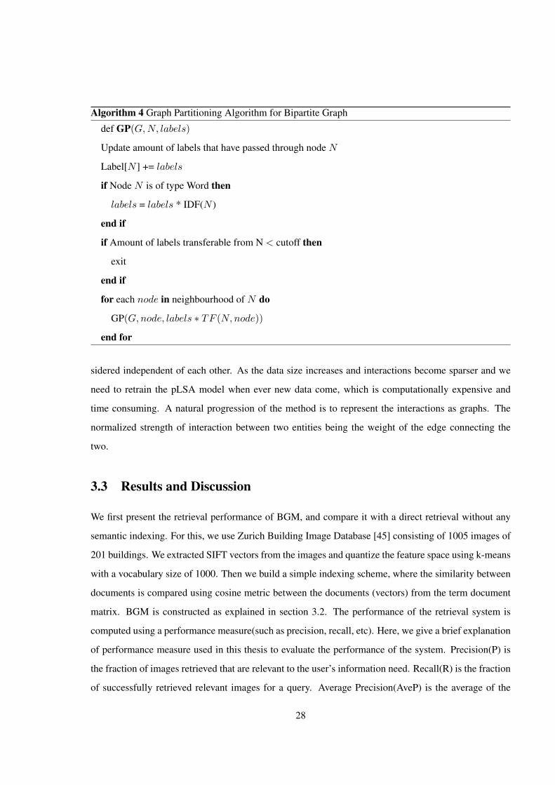
Algorithm 4 Graph Partitioning Algorithm for Bipartite Graph

def GP(G,N, labels)

Update amount of labels that have passed through node N

Label[N ] += labels

if Node N is of type Word then

labels = labels * IDF(N )

end if

if Amount of labels transferable from N < cutoff then

exit

end if

for each node in neighbourhood of N do

GP(G,node, labels ∗ TF (N,node))

end for

sidered independent of each other. As the data size increases and interactions become sparser and we

need to retrain the pLSA model when ever new data come, which is computationally expensive and

time consuming. A natural progression of the method is to represent the interactions as graphs. The

normalized strength of interaction between two entities being the weight of the edge connecting the

two.

3.3 Results and Discussion

We first present the retrieval performance of BGM, and compare it with a direct retrieval without any

semantic indexing. For this, we use Zurich Building Image Database [45] consisting of 1005 images of

201 buildings. We extracted SIFT vectors from the images and quantize the feature space using k-means

with a vocabulary size of 1000. Then we build a simple indexing scheme, where the similarity between

documents is compared using cosine metric between the documents (vectors) from the term document

matrix. BGM is constructed as explained in section 3.2. The performance of the retrieval system is

computed using a performance measure(such as precision, recall, etc). Here, we give a brief explanation

of performance measure used in this thesis to evaluate the performance of the system. Precision(P) is

the fraction of images retrieved that are relevant to the user’s information need. Recall(R) is the fraction

of successfully retrieved relevant images for a query. Average Precision(AveP) is the average of the

28

Figure 3.2: Graphical representation of Bipartite Graph Model. The image in the database is represented

as a collection of visual words. The edges connect the visual words to the images in which they are

present.

precision value obtained for the set of top t images existing after each relevant image is retrieved, and

this value is then averaged over information needs. It emphasizes ranking relevant images higher.

AveP =

∑Nr=1 P (r)× rel(r)

number of relevant images(3.1)

Here, r is the rank, N is the number of retrieved images, rel() is a binary function on the relevance of a

given rank, and P(r) precision at a given cut-off rank. Mean Average Precision(mAP) for a set of queries

is the mean of the average precision scores for each query. It has been shown to have especially good

discrimination and stability.

mAP =

∑Qq=1AveP (q)

Q(3.2)

where Q is the number of queries.

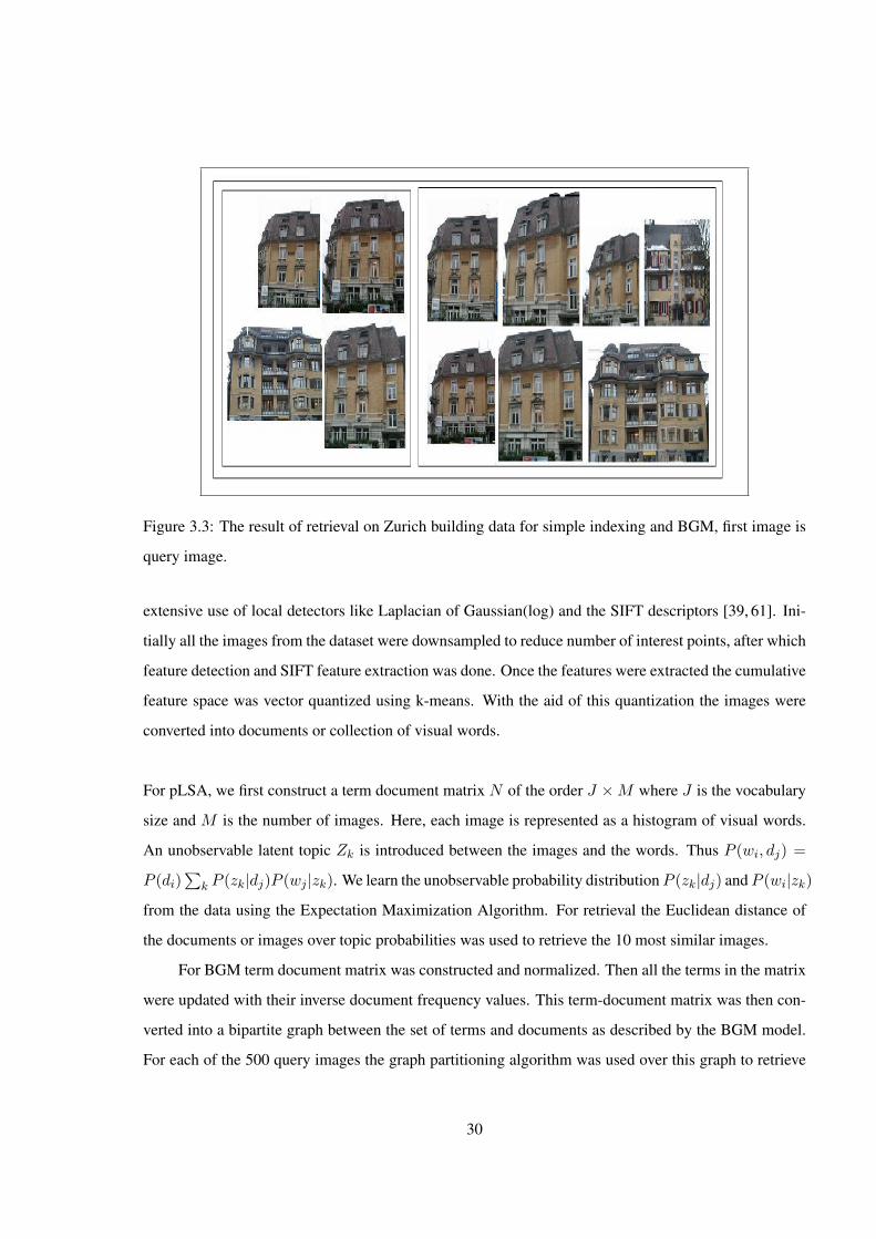
The Mean Average Precision(mAP) retrieval performance for simple retrieval is 0.26 mAP, whereas

for BGM it is 0.54 mAP. As can be seen from Figure 3.3, BGM is able to retrieve images that simple

retrieval can not. We now, compare the retrieval performance of pLSA with the retrieval performance

of BGM. For this experiment we have used holiday dataset [60], it contains 500 image groups, each

representing a different scene or object. The first image of each group is the query image and the correct

retrieval is the other images of the same group, in total the dataset contains 1491 images. We made

29

Figure 3.3: The result of retrieval on Zurich building data for simple indexing and BGM, first image is

query image.

extensive use of local detectors like Laplacian of Gaussian(log) and the SIFT descriptors [39, 61]. Ini-

tially all the images from the dataset were downsampled to reduce number of interest points, after which

feature detection and SIFT feature extraction was done. Once the features were extracted the cumulative

feature space was vector quantized using k-means. With the aid of this quantization the images were

converted into documents or collection of visual words.

For pLSA, we first construct a term document matrix N of the order J ×M where J is the vocabulary

size and M is the number of images. Here, each image is represented as a histogram of visual words.

An unobservable latent topic Zk is introduced between the images and the words. Thus P (wi, dj) =

P (di)∑

k P (zk|dj)P (wj |zk). We learn the unobservable probability distribution P (zk|dj) and P (wi|zk)

from the data using the Expectation Maximization Algorithm. For retrieval the Euclidean distance of

the documents or images over topic probabilities was used to retrieve the 10 most similar images.

For BGM term document matrix was constructed and normalized. Then all the terms in the matrix

were updated with their inverse document frequency values. This term-document matrix was then con-

verted into a bipartite graph between the set of terms and documents as described by the BGM model.

For each of the 500 query images the graph partitioning algorithm was used over this graph to retrieve

30

the 10 most similar images.

Retrieval results for the both BGM and pLSA were aggregated and the evaluation code provided

for the holiday dataset was used to calculate the Mean Average Precision(mAP) in both cases in Table

3.1.

Model mAP time space

Probabilistic LSA 0.642 547s 3267Mb

Incremental PLSA 0.567 56s 3356Mb

BGM 0.594 42s 57Mb

Table 3.1: Mean Average Precision for both BGM, pLSA and IpLSA for the holiday dataset, along with

time taken to perform semantic indexing and memory space used during indexing.

0.3 0.4 0.5 0.6 0.7 0.8

0 100 200 300 400 500 600

mA

P

No. of Concepts

mAp Vs Concepts

Figure 3.4: The retrieval performance of PLSA varying the number of Concepts.

We now demonstrate the retrieval performance of pLSA with respect to number of concepts. For

this we used Holiday database [60]. As we can see from the figure 3.4 the retrieval performance is

minimal if their is mismatch between the concepts assumed for training and the actual concepts in the

database.

Typical image retrieval systems is generally built on static databases whereas, in real world the

data keep changing i.e., the images are added or removed frequently. pLSA cannot handle stream-

31

ing/constantly changing data as the model has to be retrained on both new and old data which is com-

putationally expensive. To handle this Incremental pLSA [22] was proposed in which when ever a new

image is added, the probability of a latent topic given the document P (z|d) and the probability of words

given topic P (w|z) are updated based on Generalized Expectation Maximization [22,62]. The Table 3.1

shows the comparison of BGM with IpLSA using the evaluation code provided for the holiday dataset

for calculating the Mean Average Precision(mAP) in both cases. The mAP results show that BGM per-

forms better than IpLSA. As well as the memory usage of pLSA and IpLSA for creating the semantic

indexes(training) much higher than BGM as their space complexity is of the order O(kNz) where Nz is

the number of non-zero elements in the term document matrix and k is the number of topics.

3.4 Summary

We presented a Bipartite Graph Model(BGM) to represent the term document matrix. We also pre-

sented a Graph Partitioning algorithm for retrieving semantically relevant images from the database.

We compared the BGM with pLSA and Incremental pLSA, the experimental results shows that the re-

trieval performance of BGM is comparable to pLSA and incremental pLSA. BGM outperforms pLSA

and IpLSA in the time and memory space taken to index the images. Thus, BGM is scalable and adapts

well for dynamic databases where new images are constantly added. We also show that the retrieval

performance of pLSA and IpLSA depends on the appropriate selection of number of concepts. The next

Chapter deals with the multimodal semantic indexing techniques.

32

Chapter 4

Multi Modal Semantic Indexing

4.1 Problem Setting

Huge amount of multimedia data is available over internet. A need for effective information retrieval

systems which exploits all the data available in different modes is on raise. Here we address image

retrieval system, which using both text and content of images to improve the performance of the image

retrieval. We extended single mode semantic indexing techniques to multimodal semantic indexing.

The basic idea is to represent the image data as a 3rd- order tensor, where the first, second and third

dimensions represents images, text words and visual words respectively. First we discusses the basic

tensor concepts and then later explain our multimodal semantic indexing methods.

4.2 Tensor Concepts

A tensor is a higher order generalization of a vector(first order tensor) or a matrix (second order ten-

sor), also known as n-way array or multidimensional matrices or n-mode matrix. A tensor A can be

represented as

A ∈ RI1×I2···×IN (4.1)

Boldface lowercase letters are used to denote vectors, e.g., a. Matrices are denoted by boldface capital

letters, e.g., A. Higher-order tensors (order three or higher) are denoted by boldface calligraphic letters,

e.g., X . Scalars are denoted by lowercase letters, e.g., a. The ith entry of a vector a is denoted by ai ,

element (i, j) of a matrix A is denoted by aij , and element (i, j, k) of a third-order tensor X is denoted

33

by xijk. The norm of a tensor A ∈ RI1×I2···×IN is the square root of the sum of the squares of all its

elements, i.e.,

∥A∥ =√∑I1

i1=1

∑I2i1=1 · · ·

∑Ini1=1 a

2i1i2...in

This is analogous to the matrix Frobenius norm, which is denoted ∥A∥ for a matrix A. The scalar

product ⟨A,B⟩ of two tensor A,B is defined as

⟨A,B⟩ =∑I1

i1=1

∑I2i1=1 · · ·

∑Ini1=1 ai1i2...inbi1i2...in

Thus,∥A∥ =√

⟨A,A⟩. The mode-d metricizing or matrix unfolding of an N th order tensor A ∈

RI1×···×IN are vectors in RNd obtained by keeping index d fixed and varying the other indices. There-

fore, the mode-d matricizing A(d) is in R(Πi=dNi)×Nd . Tensor element (i1, i2, . . . , iN ) maps to matrix

element(in, j) where j = 1 +∑N

k=1,k =n(ik − 1)jk with jk = Πk−1m=1,m =nIm

See [63] for details on matrix unfolding of a tensor. Higher Order SVD(HOSVD) is an extension

of SVD and represented as follows

A = Z ×1 U1 ×2 U2 · · · ×N UN (4.2)

where U1, U2, . . . , UN are orthogonal matrices that contain the orthonormal vectors spanning the col-

umn space of the matrix unfolding A(i) with i = 1, 2, . . . , N . Z is a core tensor, analogous to the

diagonal singular value matrix in conventional SVD as shown in Figure 4.1 HOSVD is computed by the

following two steps.

1. For i = 1, 2, . . . N, compute the unfolding matrix A(i) from A and compute its standard SVD:

A(i) = USVH; the orthogonal matrix U(i) is defined as U(i) = U, i.e., as the left matrix of

SVD on A(i).

2. Compute the core tensor using the inversion formula

Z = A×1 U(1)H ×2 U

(2)H · · · ×p U(p)H (4.3)

where the symbol H denote the Hermitian matrix transpose operator.

Tensor methods have been used for a long time in chemometrics and psychometrics [64]. Recently

HOSVD has been applied to face recognition [65], Handwritten digit classification [66] and data mining

[67].

34

4.3 Multi Modal Latent Semantic Indexing

The term-document matrix is a high dimensional representation of the image in which each image

is represented as frequency of the visual words. In retrieval domain most of the systems are based on

direct matching of the visual words. However generally, different visual words are used to describe same

concepts or different concepts are described using similar visual words because of which direct matching

of visual words may not lead to efficient retrieval systems. LSI tries to search relevant documents by

mapping high dimensional vector to a low dimensional latent semantic space. Thus removing the noise

found in images, such that two documents that have same semantics will be located close to one another

in a multi-dimensional space. Most of the current image representations either rely solely on visual

features or on surrounding text.

Matrix decomposition techniques like singular value decomposition(SVD), Principal component

analysis(PCA) etc are useful for dimensionality reduction, mining, information retrieval and feature

selection. But these are limited to two orders only. Generally most of the data have a multidimensional

structure and it is some what unnatural to organize them as matrices or vectors. For example a video

is a collection of images and audio over a time stamp. Thus in many cases it is beneficial to use

the available data without destroying its inherent multidimensional structure. Our tensor based model

capture information for more than two orders where tensor is multidimensional or multimode arrays.

In [14], author shows the effect of LSA on Multimedia document indexing and retrieval by combin-

ing both text and image. Here, they concatenate the columns of the two matrices NM×Nt and NM×Nv

(M number of images , Nt number textwords and Nv number of visual words in the database) into a

single term document matrix and then decompose into reduced dimension to form a latent space. But

this does not lead to desired improvement in retrieval results because the visual words have a much

larger frequency as compared to text words. The difference in the dictionary size for the two is large

as well. To overcome the above disadvantages, we propose MMLSI , where the data is represented

by a 3-order tensor in which the first dimension is images, second is visual words and the third is the

text words. Three-mode analysis using Higher Order Singular Value Decomposition (HOSVD) [63] is

performed on the 3-order tensor which captures the latent semantics between multiple objects like im-

ages, low-level features and surrounding text. HOSVD technique can find some underlying and latent

structure of images and is easy to implement. It helps to find correlated dimensions within the same

mode and across different modes.

35

Figure 4.1: The figure shows visual word - text word - document tensor and its decomposition

As we are considering two modes, first we construct a tensor A ∈ RI1XI2XI3 where, I1 is the

number of the images in the dataset, I2 is the visual vocabulary size and I3 is the text vocabulary size.

Whereas, aijk is defined as number of occurrences of visual word vj and text word tk in a document di.

Once the tensor is generated we decompose it by using HOSVD as shown in Figure 4.1 to obtain

A = Z ×1 Uimages ×2 Uvisualwords ×3 Utextwords.

Here the, the matrices Uimages, Uvisualwords and Utextwords define the space of the image parame-

ters, visual parameters and textual parameters respectively. An approximate tensor is constructed A by

selecting the top k columns from the decomposed matrices. This in effect maps the data into a semantic

space, which is derived from the multiple data modes. The semantic space has a lower dimension than

the dictionary space. Hence in effect mapping the data into a lower dimensional space.

4.4 Semantic Indexing By Multi-Modal pLSA

Although LSA has been successfully applied for semantic analysis for various applications like Infor-

mation retrieval, image annotation and object categorizing. It has a number of disadvantages mainly due

36

to its unsatisfactory statistical foundation. Where as, pLSA is a generative model of the data with strong

statistical foundation, as it is based on the likelihood principle. It has found successful applications in

single mode data such as text analysis and image analysis. In [13], author shows the dimensionality

reduction due to the aspect model of pLSA which improves the performance on similarity task for a

large data bases.

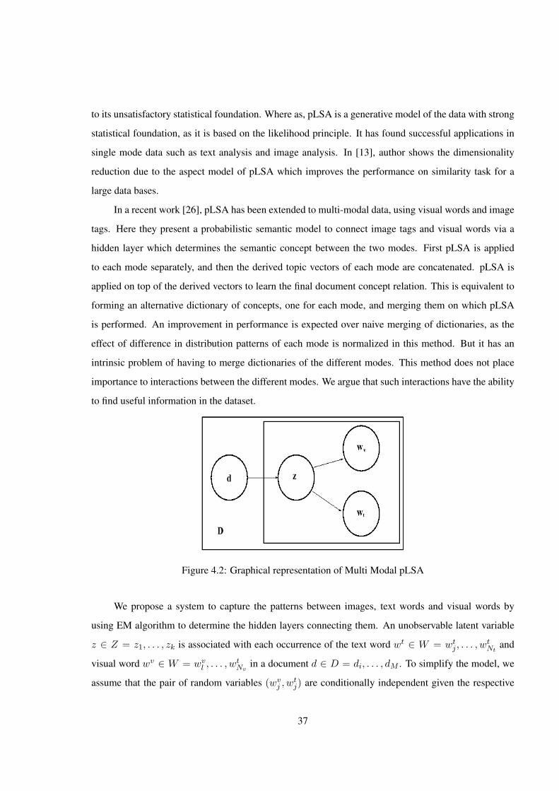
In a recent work [26], pLSA has been extended to multi-modal data, using visual words and image

tags. Here they present a probabilistic semantic model to connect image tags and visual words via a

hidden layer which determines the semantic concept between the two modes. First pLSA is applied

to each mode separately, and then the derived topic vectors of each mode are concatenated. pLSA is

applied on top of the derived vectors to learn the final document concept relation. This is equivalent to

forming an alternative dictionary of concepts, one for each mode, and merging them on which pLSA

is performed. An improvement in performance is expected over naive merging of dictionaries, as the

effect of difference in distribution patterns of each mode is normalized in this method. But it has an

intrinsic problem of having to merge dictionaries of the different modes. This method does not place

importance to interactions between the different modes. We argue that such interactions have the ability

to find useful information in the dataset.

Figure 4.2: Graphical representation of Multi Modal pLSA

We propose a system to capture the patterns between images, text words and visual words by

using EM algorithm to determine the hidden layers connecting them. An unobservable latent variable

z ∈ Z = z1, . . . , zk is associated with each occurrence of the text word wt ∈ W = wtj , . . . , w

tNt

and

visual word wv ∈ W = wvl , . . . , w

tNv

in a document d ∈ D = di, . . . , dM . To simplify the model, we

assume that the pair of random variables (wvj , w

tj) are conditionally independent given the respective

37

image or document di. Thus

P (wvl |wt

j , di) = P (wvl |di) (4.4)

Now consider a joint probability model for text words, images or documents and visual words as

P (wtj , di, w

vl ) = P (wt

j)P (wtj |di)P (wv

l |wtj , di) (4.5)

By substituting equation 4.4, equation 4.5 can be reduced to

P (wtj , di, w

vl ) = P (di)P (wt

j |di)P (wvl |di) (4.6)

Where, P (wtj |di) probability of occurrence of text word wt

j given a document di, similarly P (wvl |di)

probability of occurrence of visual word wvl given a document di. Generally, documents consist of mix-

ture of multiple topics, and occurrences of words (i.e., visual words and text words) is a result of topic

mixture. The generative model is expressed in terms of the following features:

1. pick a latent class zk with probability P (zk|di).

2. generate a text word wtj with probability P (wt

j |zk).

3. generate a visual word wvl with probability P (wv

l |zk)

The joint probabilistic model for the above generative model is given by the following:

P (wtj , di, w

vl ) = P (di)

∑k

P (wtj |zk)P (zk|di)P (wv

l |zk)P (zk|di) (4.7)

=P (di)

2∑

k P (wtj |zk)P (wv

l |zk)P (zk|di)2

P (zk)(4.8)

The Figure 4.2 shows the pictorial representation of the model. Here the a combination of text

words and visual words is used to represent the image upon which higher level aspects are learned.

By following the Maximum likelihood principle we can determine P (zk|di), P (wtj |zk) and P (wv

j |zk)

by maximizing the log-likelihood function.

L = ΠMi=1Π

Nt

j=1ΠNv

l=1[P (wtj , di, w

vl )

n(wtj ,di,w

vl )] (4.9)

Taking the log to determine the log-likelihood L of the database

L =M∑i=1

Nt∑j=1

Nv∑l=1

[n(wtj , di, w

vl )P (wt

j , di, wvl )] (4.10)

38

By substituting the equation 4.8 in equation 4.10 we learn the unobservable probability distribution

P (zk|di), P (wtj |zk) and P (wv

j |zk) from the data using the Expectation-Maximization Algorithm (EM-

Algorithm): [46]

E-Step:

P (zk|di, wtj) =

P (wtj |zk)P (zk|di)∑k

n=1 P (wtj |zn)P (zn|di)

(4.11)

P (zk|di.wvl ) =

P (wvl |zk)P (zk|di)∑k

n=1 P (wvl |zn)P (zn|di)

(4.12)

M-Step:

P (wtj |zk) =

∑Mi=1 n(di, w

tj)P (zk|di, wt

j)∑Nj=1

∑Mi=1 n(di, w

tj)P (zk|di, wt

j)(4.13)

P (wvl |zk) =

∑Mi=1 n(di, w

vl )P (zk|di, wv

l )∑Ll=1

∑Mi=1 n(di, w

vl )P (zk|di, wv

l )(4.14)

P (zk|di) =∑N

j=1

∑Ll=1 n(di, w

tj , w

vl )P (zk|di, wt

j)P (zk|di, wvl )

n(di)(4.15)

The learning process is iterating the E-Step and M-Step alternatively until some convergence con-

dition (such as Log likelihood) is satisfied. Typically, 100-150 iterations are needed before converging.

Thus finally images are mapped to a lower dimensional latent vector derived from both text words

and visual words. In the next section we discuss how the proposed indexing methods can be used for

multi-modal image retrieval.

4.5 Indexing and Retrieval

As mentioned earlier many current retrieval system depends on either text or visual features. But in many

cases information available is richer and is available as a combination of different modes. For example

any web page contains text, imagery and other forms of information. The research in these modalities is

well established like [23] builds a system using visual words, where as commercials systems like flickr

user text words. But the retrieval effectiveness is bottleneck by semantic gap(See 1.1.3). In recent years,

research has been done to address semantic gap problem, but these methods fail to relate an image to

an abstract concept. Thus, an image retrieval system which focuses on exploiting the synergy between

different modes helps in improving the retrieval efficiency.

39

4.5.1 Feature Extraction

Visual Vocabulary For a given image, first interest points are detected from which feature vectors

are extracted. Once the features were extracted the cumulative feature space was vector quantized into

clusters. These clusters form the visual words and each image is represented as a histogram of visual

words.

Textual Vocabulary For the textual representation of each image, the keywords were extracted from

the corresponding annotated text by removing stop words and stemming the remaining words. Thus

for each image the key text words were found and the dataset is represented as term-document matrix.

Thus, the visual words and key words forms the two modes of the documents.

Figure 4.3: Over view of the Process

4.5.2 Image Retrieval Framework

For a tensor based image retrieval, a multi modal framework is used to combine multiple modes to gen-

erate an image retrieval system as shown in section 4.3. Here, first we need to construct a tensor A from

40

the dataset. Once the feature extraction is done, image are represented as histogram of visual words and

histogram of keywords. A Tensor A is constructed by the following equation

A(i, j, l) = n(di, wtj) · (1− α) + n(di, w

vl ) · (α).

Where, n(di, wtj) specifies the number of time the text word wt

j occurred in a document di and

n(di, wvl ) specifies the number of times the visual word wv

l occurred in a document di. This is based on

the amount of information each mode has. We choose α such that the resulting matrix has a distribution

which balances the effect of the multiple modes on the semantic generation. An efficient process to

find an optimal α is beyond the scope of the current discussion. Then tensor A is decomposed using

HOSVD as explained in section 4.3. From resulting decomposition select the top k columns to form a

reduced dimensional space. The reconstructed tensors is denoted by

A = Z ×1 Uimages ×2 Uvisualwords ×3 Utextwords

The database image and the queries are mapped on to the 2 base Uvisualwords and Utextwords. And

a Euclidean distance between them is calculated to rank the relevance of the images. see Algorithm 5

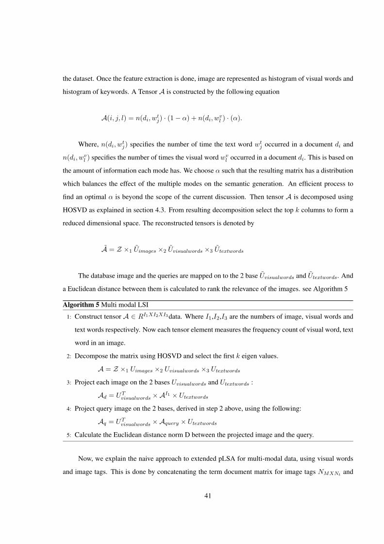
Algorithm 5 Multi modal LSI

1: Construct tensor A ∈ RI1XI2XI3data. Where I1,I2,I3 are the numbers of image, visual words and

text words respectively. Now each tensor element measures the frequency count of visual word, text

word in an image.

2: Decompose the matrix using HOSVD and select the first k eigen values.

A = Z ×1 Uimages ×2 Uvisualwords ×3 Utextwords

3: Project each image on the 2 bases Uvisualwords and Utextwords :

Ad = UTvisualwords ×AI1 × Utextwords

4: Project query image on the 2 bases, derived in step 2 above, using the following:

Aq = UTvisualwords ×Aquery × Utextwords

5: Calculate the Euclidean distance norm D between the projected image and the query.

Now, we explain the naive approach to extended pLSA for multi-modal data, using visual words

and image tags. This is done by concatenating the term document matrix for image tags NMXNt and

41

visual words NMXNv into NMX(Nt+Nv) and then applying standard pLSA [26]. But this does not show

any improvement in the quality of retrieval for average case scenario. The performance invariance is

caused because the visual words have a much larger frequency as compared to text words and the dif-

ference in the dictionary size for the two is large. Another basic approach is to apply pLSA on term

document matrix for image tags NMXNt and visual words NMXNv separately and then the results are

combined using set operations like union or intersection. The problem to determine the weights of the

text and visual words is not trivial.

For image retrieval system based on Multi modal pLSA, the topic specific distributions P (wtj |zk)

and P (wvl |zk) are learnt from the set of training images according to the method explained in section 4.4.

Each training image is then represented by a Z-vector P (zk|dtrain), where Z is the number of topics

learnt. Using the same approach, given a new test image dtest we estimate the aspect probabilities

P (zk|dtest). The probabilities P (wtj |zk) and P (wv

l |zk) learned from train set are kept constant. The

similarity between the test and training images is calculated using the cosine metric between the two

aspect vectors a = (P (zk|dtrain)) and b = (P (zk|dtest))(see Algorithm 6).

Algorithm 6 Multi modal pLSA

1: • Training Phase:

2: Randomize and normalize P (wtj |zk), P (zk|di), and P (wv

l |zk) to ensure the sum of all probabilities

equal to one.

3: while not convergence do

4: E-step: Compute the posterior probabilities P (zk|di, wtj) and P (zk|di, wv

l ).

5: M-step: Parameters P (wtj |zk), P (zk|di), and P (wv

l |zk) are updated from the posterior probabil-

ities computed in E-step.

6: end while

7: • Testing Phase:

8: The E-step and M-step are applied on the testing data by keeping the probabilities P (wtj |zk) and

P (wvl |zk) learnt from the training constant.

9: Calculate the cosine metric between the probabilities learnt from training and testing.

42

4.6 Results and Discussions

In this section, we present the various experimental results for the proposed MultimodeLSI and

MultimodepLSA on the datasets described below.

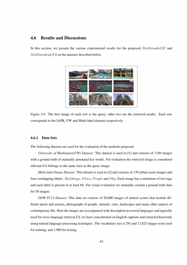
Figure 4.4: The first image of each row is the query, other two are the retrieved results. Each row

corresponds to the IAPR, UW and Multi-label datasets respectively

4.6.1 Data Sets

The following datasets are used for the evaluation of the methods proposed.

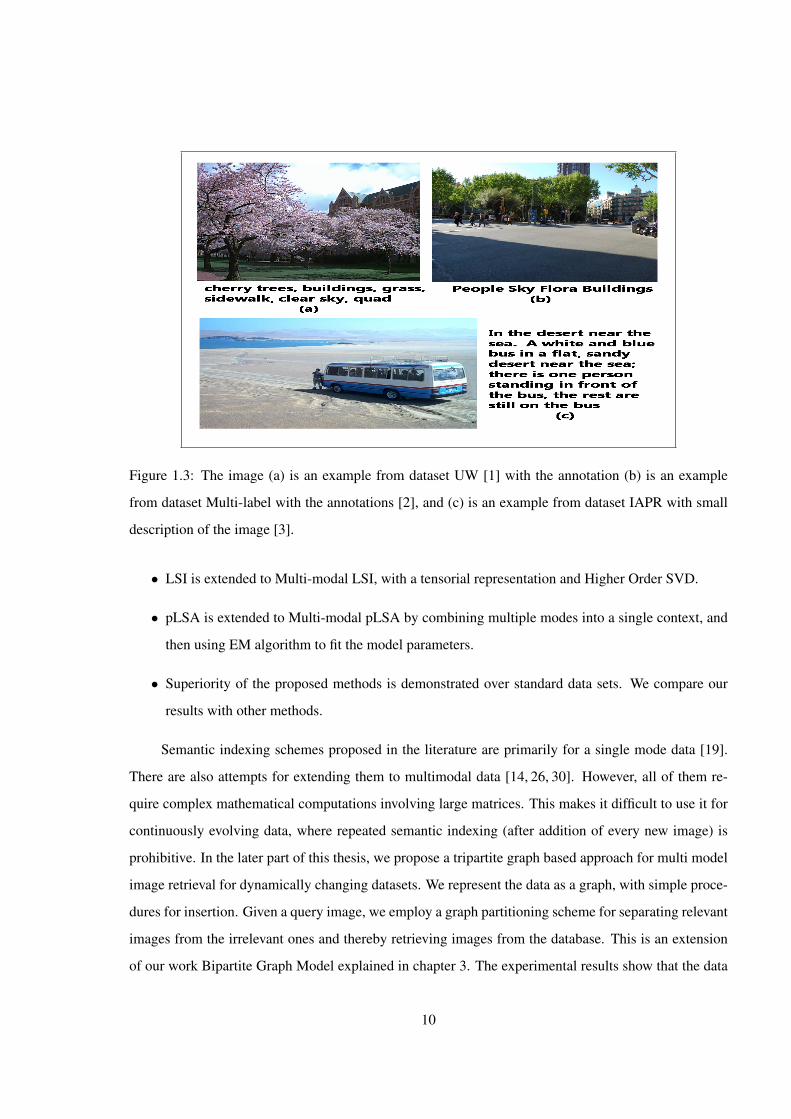
University of Washington(UW) Dataset: This dataset is used in [1] and consists of 1109 images

with a ground truth of manually annotated key words. For evaluation the retrieved image is considered

relevant if it belongs to the same class as the query image.

Multi-label Image Dataset: This dataset is used in [2] and consists of 139 urban scene images and

four overlapping labels: Buildings, Flora, People and Sky. Each image has a minimum of two tags

and each label is present in at least 60. For visual evaluation we manually created a ground truth data

for 50 images.

IAPR TC12 Dataset: This data set consists of 20,000 images of natural scenes that include dif-

ferent sports and actions, photographs of people, animals, cites, landscapes and many other aspects of

contemporary life. Here the images are accompanied with description in several languages and typically

used for cross-language retrieval [3], we have concentrated on English captions and extracted keywords

using natural language processing techniques. The vocabulary size is 291 and 17,825 images were used

for training, and 1,980 for testing.

43

Table 4.1: Comparing Multi Modal LSI with different forms of LSI for all the datasets in mAP.

Datasets visual-based tag-based Pseudo single mode MMLSI

UW [1] 0.46 0.55 0.55 0.63

Multilabel [2] 0.33 0.42 0.39 0.49

IAPR [3] 0.42 0.46 0.43 0.55

Corel [68] 0.25 0.46 0.47 0.53

Corel Dataset: This dataset is used in [68] which consists of 5000 images out of which 4500

images are used for training and 500 image for testing. The dictionary contains around 260 unique

words. The retrieved image is considered relevant if it belongs to the same class as the query image.

Table 4.2: Comparing Multi Modal PLSA with different forms of PLSA for all the datasets in mAP.

Datasets visual-based tag-based Pseudo single mode mm-pLSA our MM-pLSA

UW [1] 0.60 0.57 0.59 0.68 0.70

Multilabel [2] 0.36 0.41 0.36 0.50 0.51

IAPR [3] 0.43 0.47 0.44 0.56 0.59

Corel [68] 0.33 0.47 0.48 0.59 0.59

4.6.2 Experimental Results

Initially all the images from the datasets were down sampled to reduce number of interest points, after

which feature detection and SIFT feature extraction [39] is applied. For corel dataset we calculated

dense sift. Then the features are vector quantized using k-means. For our experiments we created a

visual vocabulary size of 500 for all the datasets, except for IAPR for which the vocabulary size is 1000.

For benchmarking, we compared our method against the following classes of modes:

• Single mode: This refers to methods that consider only a single mode throughout the process

[13, 45]. For example text only and visual words only methods lie in this category

• Pseudo single mode: This category of applications use single mode methods, but can use data

from multiple modes. One of the approach to do so is to merge the dictionaries [26,68]. Hence in

effect all the modes present in the dataset are considered as a single mode. This merged mode is

44

then processed by single mode methods. This is a naive way of managing multimode data. The

disadvantages include shadowing of one mode by another by factors that include dictionary size,

distribution etc. As these factors are crucial in the performance of single mode methods, very

little advantage can be gained out of such a method.

• Explicit dual mode: These methods are designed so as to appreciate the diversity in the semantics

of information represented by each mode. For example, one mode can have a small dictionary,

but the distribution is such that the semantics can be easily found, another might have a much

larger dictionary, but the average vocabulary per document is small. One such method present in

literature is that of multi-modal multi-layer pLSA [26].

In the current context, visual words and text words are the two modes we have focused upon. For single

mode methods, either of text or visual words is used. For Pseudo dual mode methods, the dictionaries

are concatenated. The resulting dictionary is then used. For example, for the IAPR dataset, the visual

dictionary is of size 500, and the text dictionary is of size 291, hence the resulting dictionary is of size

791, with the first 500 representing the visual words.

As discussed in the previous sections, LSI and pLSA based methods are compared in different

modes. For all our experiments the number of concepts is determined by the concepts present in the

respective databases which is known. We use mean Average precision (mAP) for comparison. The

results of the experiments are as shown below:

LSI and variants: Compared to variants of LSI, our method performs better see Table 4.1. It is

to be noted that a better tag base has a stronger impact on accuracy of results as compared to a better

visual word. This can possibly be because most key text words are found only in a very few documents,

and are related to each other very strongly. Also, concatenation of the two together did not provide any

appreciable performance improvements, in some cases accuracy reduced below that of tag based LSI.

The values derived are heavily biased towards the results obtained from the tags alone. Thus proving our

proposition. The results obtained by our method are stronger than the other results, but on the contrary

the time and space consumption for our method is much larger than the others.

pLSA and variants: A similar direct comparison shows us that other than the Corel data set. The

results of concatenated pLSA are dominated by the results of visual word based pLSA. Similar to the

LSI models here we construct a pLSA model solely based on visual features or tags and a concatenated

plSA model. Then we implemented a Fast Initialization variant of multi modal multi layer pLSA(mm-

45

pLSA) proposed in [26]. The Table 4.2 shows the comparison of these methods with the proposed Multi

model pLSA. Our method outperforms current single mode and multimode methods in performance.

From the two Tables 4.1 and 4.2 we can see that the performance of the probabilistic methods is

better than the Latent semantic analysis. It can also be seen that methods that efficiently make use of

multiple modes of information are able to generate better semantics. An obvious problem with such

methods is the time taken to update the model given a dynamic database. Hence the focus can be on

efficient methods to manage dynamic multimodal data. Thus methods that generate just in time results

on a dynamic database are required.

4.7 Summary

We extended two semantic indexing techniques LSI and pLSA for mutlimodal semantic indexing. Here

the data is represented as 3rd-order tensor, where the first dimension is images, second dimension is text

words and the third dimension is visual words. Then matrix decomposition or probabilistic techniques

are applied to learn inherent concepts. Thus the images are mapped to a concept space. For retrieval,

the query images are also mapped to concept space in the same fashion. A distance matric is computed

between the trained images and the query images, and results are presented in a ranked order. The

experimental results shows that, the proposed methods outperforms current single mode and multimode

methods. But similar to LSI and pLSA these methods are also expensive in memory and computation.

The next chapter deals with the representation of the multimodal data using graph based modal. This

method is scalable to large and dynamic image databases. Retrieval is done using a graph partitioning

algorithm.

46

Chapter 5

Tripartite Graph Modal

5.1 Problem Setting

The disadvantage with Semantic Indexing techniques is with resource usage. In MMLSI, the HOSVD

algorithm, the orthonormal matrices in the Equation 4.2 are in practice computed from the SVD of the

unfoldings of A(i)(See 4.2). Thus, the computational complexity of HOSVD is similar to SVD i.e.,

O(T 2 · k3), where T is the number of visual terms or text terms plus documents, and k is the number of

dimensions in the concept space. Similarly in MMpLSA, the EM algorithm takes O(R · k) operations

for each iteration. Where R is number of distinct observation of triads of text terms, visual term and

documents. i.e, I1 × I2 × I3 times the degree of sparseness of the term-document tensor. Here I1 is the

number of documents or images and I2 are number of visual terms and I3 are the number of text terms.

Typically in both cases, k will be small. Similar to LSI and pLSA, MMLSI and MMpLSA are unfeasible

for a large, dynamic collection(See 3.1). And also determining the optimal number of dimensions in the

concept space is another problem encountered. To address this issues we present a graph based model

which is an extension of bipartite graph model(See 3.2) in this chapter.

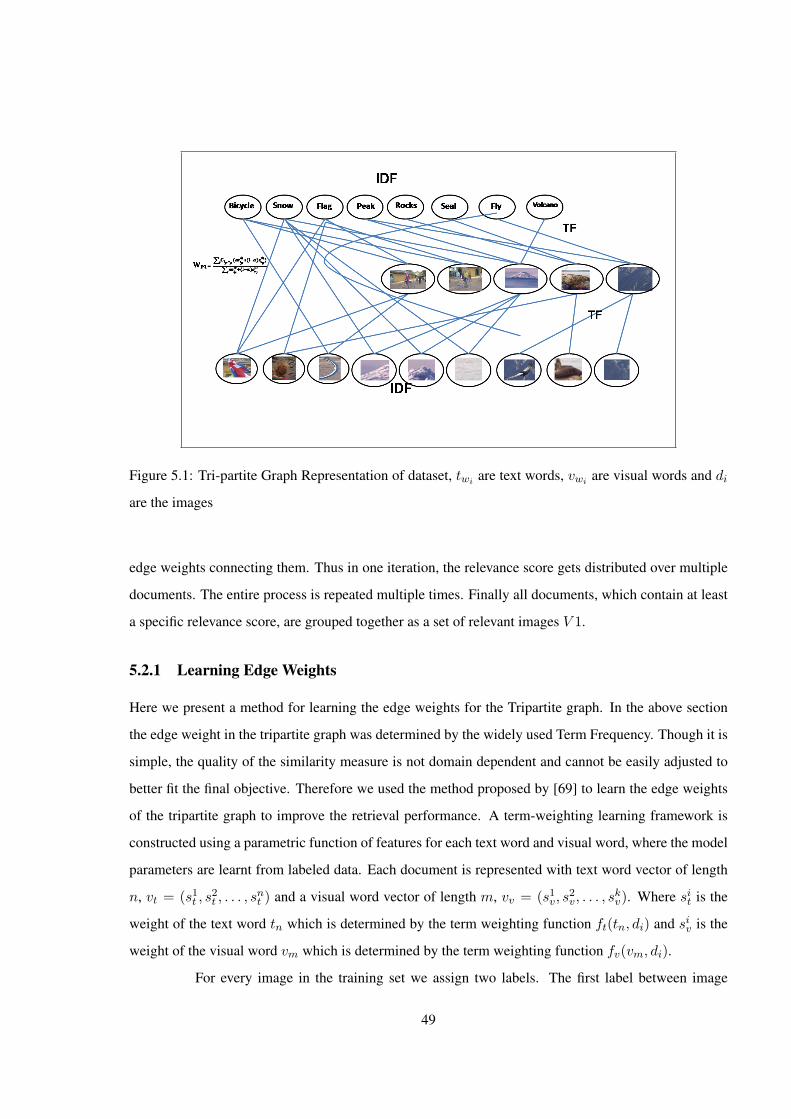
5.2 Tripartite Graph Representation and Retrieval

The basic idea, here, is to encode the tensorial representation as a Tripartite graph of text words, visual

words and images. An undirected tripartite graph G = (T, V,D,E) has three sets of vertices where,

T = {t1, t2 . . . , tn} are text words, V = {v1, v2 . . . , vm} are visual words and D = {d1, d2 . . . , di} are

images with E = {ed1t1 , .., editn , e

d1v1 , .., e

divm , e

t1v1 , .., e

tnvm} as set of edges. Figure 5.1 shows pictorially rep-

47

resent the tripartite graph model (TGM) we use. Thus this model has three sets of vertices (images, text

words and visual words) and edges going from one set to other. The nodes correspond to visual words as

well as text words store the inverse document frequency (IDF) corresponding to the document(image)

collection. The edges from text words to images as well as those from visual words to images, encode

the term frequency (TF) corresponding to the word-image pair. However, the weights of edges which

relate the text words with visual words can not be directly assigned. These edges are weighed as:

Wpq =

∑iCtp,vp(αe

ditp + (1− α)edivq)∑

i αeditp + (1− α)edivq

Where Ctp,vq = 1, if tp and vq are there in document di. Since the documents (images) are the entity

which connects text words and visual words, summations are carried out over the images/documents.

For indexing, a tripartite graph G is constructed with the nodes and edges as mentioned above. Given

a collection of images and textual tags, building a TGM is possible. However, when additional im-

ages come, TGM shows its advantage in insertion. To insert an additional image, the TF and IDFs are

computed with the new document. We assume the vocabularies to be static. This insertion is computa-

tionally light. For retrieval, we partition the vertex set D of G into two vertex sets (V 1, V 2), such that

vertex set V 1 contains documents which are relevant to the query, and V 2 contains all other nodes. This

is done as explained below.

When a query image is given, query node attaches itself to the nodes in the set T and V which are

directly related to the query, with the relationship previously known. Our objective now is to identify

similar images to the query, which are already indexed. The nodes initially contains a relevance score

(R) which is partitionable. The nodes then distributes the relevance score based on the edge weight

between the nodes and its neighbours, such that the received amount of score is directly proportional to

the edge weight. The neighbours then propagate the relevance score to their neighbours. If the node is

a document node, the distribution of the relevance score among its edges is determined according to the

quantity which is proportional to the flow capacity calculated by the normalized Term Frequency (TF)

value. If the node is a text word or visual word node and its neighbour node is document node, then a

penalty, which is proportional to the Inverse document Frequency(IDF) value of the word, is taken from

the amount of relevance score it receives and the rest is distributed like the document node based on

the flow capacity of its edges. Hence higher the edge weights the more relevance score is propagated

to the relevant node. The relevance score is propagated between the text and visual words based on the

48

Figure 5.1: Tri-partite Graph Representation of dataset, twi are text words, vwi are visual words and di

are the images

edge weights connecting them. Thus in one iteration, the relevance score gets distributed over multiple

documents. The entire process is repeated multiple times. Finally all documents, which contain at least

a specific relevance score, are grouped together as a set of relevant images V 1.

5.2.1 Learning Edge Weights

Here we present a method for learning the edge weights for the Tripartite graph. In the above section

the edge weight in the tripartite graph was determined by the widely used Term Frequency. Though it is

simple, the quality of the similarity measure is not domain dependent and cannot be easily adjusted to

better fit the final objective. Therefore we used the method proposed by [69] to learn the edge weights

of the tripartite graph to improve the retrieval performance. A term-weighting learning framework is

constructed using a parametric function of features for each text word and visual word, where the model

parameters are learnt from labeled data. Each document is represented with text word vector of length

n, vt = (s1t , s2t , . . . , s

nt ) and a visual word vector of length m, vv = (s1v, s

2v, . . . , s

kv). Where sit is the

weight of the text word tn which is determined by the term weighting function ft(tn, di) and siv is the

weight of the visual word vm which is determined by the term weighting function fv(vm, di).

For every image in the training set we assign two labels. The first label between image

49

and each visual word is denoted as {(y1, (v1, d1)), (y2, (v2, d1)), (y3, (v1, d2)) . . . , (ymxi, (vm, di))}.

The label ymxi is the visual term frequency of vm in the image di. and second label between image

and each text word, is denoted as {(h1, (t1, d1)), (h2, (t2, d1)), (h2, (t2, d1)), . . . , (hnxi, (tn, di))}. The

label hnxi is the text term frequency of the tn in the images di. A parametric function of features for

each visual word and text word are calculated separately.

Then we use general loss functions sum-of-squares error and log loss to learn the model parameter

by using L-BFGS for fast convergence and local minima as described in [69]. The final value of ykxm

and hnxm gives the relevance between the image and the corresponding visual words and text words

respectively, which can be considered as the weights of the Tripartite graph. Then we apply graph

partitioning algorithm as mentioned in the above section 5.2.

5.2.2 Offline Indexing

Here we discuss Bipartite graph model as a special case of TGM. An offline indexing technique for

BGM is presented to reduce the computational time for retrieval. In BGM, the edges are weighted with

term frequencies of words in the documents and each term is also associated with an inverse document

frequency value. These values determine the relevance of a word in a particular image. We use graph

comparison method in [70] to obtain the similarity between images. Here, first we present some basic

definitions and then explain how graph comparison method is used for computing similarity between

images.

A similarity matrix S is computed between two graphs GA and GB as a limit of the normalized

even iterates of Sp+1 = BSpAT + BTSpA, where A and B are the adjacency matrix of GA and GB

respectively. The entry sxy in similarity matrix S gives the similarity score between a vertex x in GA to

a vertex y in GB . A special case is GA =GB=G′, where G′ is a graph. The similarity matrix S gives

similarity scores between vertices of G′, which is self similarity matrix of G′. Truong et al. [70] shows

the application of this for document retrieval. Here we demonstrate this for image retrieval. The values

for the similarity matrix can be either initialized to a known prior knowledge between the vertices’s of

the graphs or same similarity values. Let M be the adjacency matrix of a bipartite graph G where the

vertices’s have been ordered such that the first i rows are the number of images in D and last m rows are

50

the visual words in W. The initial values of the similarity matrix is computed as follows:

S0(x, y) =

∑p=1→i+m

M(x, p) ·M(y, p)√ ∑p=1→i+m

M(x, p) ·M(y, p) ∗√ ∑

p=1→i+m

M(x, p) ·M(y, p)

(5.1)

The S0 can be written as

SW 0

0 SD

where SW is the m×m visual word similarity matrix and SD

is the i× i image similarity matrix.

Sp+1 =

LtLSWpLtL 0

0 LtLSDpLtL

√

∥LtLSWpLtL∥2 + ∥LtLSDpL

tL∥2(5.2)

Where L is the term document matrix. Iterating the equation 4 until convergence is achieved will result

in a similarity matrix Sp which gives the similarity measure between the images in the graph G.

5.3 Results and Discussions

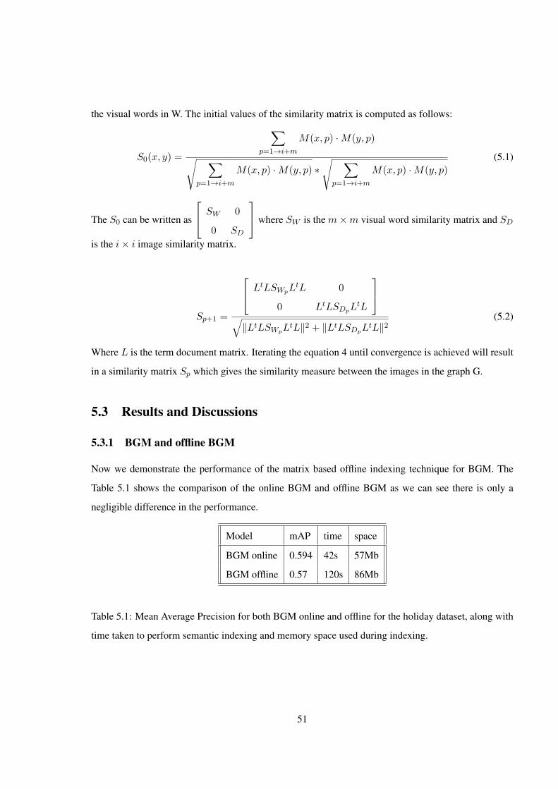
5.3.1 BGM and offline BGM

Now we demonstrate the performance of the matrix based offline indexing technique for BGM. The

Table 5.1 shows the comparison of the online BGM and offline BGM as we can see there is only a

negligible difference in the performance.

Model mAP time space

BGM online 0.594 42s 57Mb

BGM offline 0.57 120s 86Mb

Table 5.1: Mean Average Precision for both BGM online and offline for the holiday dataset, along with

time taken to perform semantic indexing and memory space used during indexing.

51

5.3.2 Multimodal Retrieval

In this section, we present the experimental results for the proposed TGM and compare with the other

Multimodal retrieval systems. We used four datasets for the evaluation of the methods proposed. Univer-

sity of Washington(UW) Dataset: This dataset is used in [1] and consists of 1109 images with a ground

truth of manually annotated key words. For evaluation the retrieved image is considered relevant if it

belongs to the same class as the query image. Multi-label Image Dataset: This dataset is used in [2] and

consists of 139 urban scene images and four overlapping labels: Buildings, Flora, People and Sky.

For visual evaluation we manually created a ground truth data for 50 images. IAPR TC12 Dataset: This

data set consists of 20,000 images of natural scenes. Here the images are accompanied with description

in several languages and typically used for cross-language retrieval [3], we have concentrated on English

captions and extracted keywords using natural language processing techniques. The vocabulary size is

291 and 17,825 images were used for training, and 1,980 for testing. NUS-WIDE [71]: It consist of

269,648 images and the associated tags from Flickr, with a total number of 5,018 unique tags. Initially

Table 5.2: Comparing TGM with Multi Modal LSI and Multi Modal pLSA for different the datasets

Datasets MMLSI MMpLSA mm-pLSA TGM-TFIDF TGM-learning

UW [1] 0.63 0.70 0.68 0.64 0.67

MultiLable [2] 0.49 0.51 0.50 0.49 0.50

IAPR [3] 0.55 0.59 0.56 0.56 0.59

NUS-WIDE [71] 0.33 0.39 0.37 0.35 0.38

all the images from the datasets were down sampled to reduce number of interest points, after which

feature detection and SIFT feature extraction [39] is applied. Now the features are vector quantized us-

ing k-means. For our experiments we created a visual vocabulary size of 500 for all the datasets, except

for IAPR for which the vocabulary size is 1000.

We implemented Multi modal LSI(MMLSI) and Multi Modal pLSA(MMpLSA) as explained in

section 4.3. The latent concept k is set to the value specified in the dataset. We also implemented

a multi-layer multi modal pLSA as explained in [26]. An improvement in performance is expected

over naive merging of dictionaries, as the effect of difference in distribution patterns of each mode is

normalized in this method. However, it has an intrinsic problem of having to merge dictionaries of the

different modes. This method does not place importance to interactions between the different modes.

52

We argue that such interactions have the ability to find useful information in the dataset.

A TGM with edge weights as TF and as weighted-learning is constructed for all the datasets as

explained in sections 5.2 and 5.2.1 respectively. Table 5.2 shows the comparison of these methods in

mean Average Precision(mAP) values. For all our experiments the number of concepts is determined by

the concepts present in the respective databases that are known. The mAP results show that performance

of TGM is comparable to other methods. The performance of TGM with weighted-learning is slightly

better that with the TF. The advantage of TGM is noticeable when new images are added to database.

As we can see in Table 5.3 TGM takes only few milliseconds for semantic indexing whereas for variants

of pLSA the entire semantic indexing needs to be done again, incurring high time and memory costs.

Model mAP time space

MMLSI 0.63 1897s 4856Mb

MMpLSA 0.70 983s 4267Mb

mm-pLSA 0.68 1123s 3812Mb

TGM 0.67 55s 168Mb

Table 5.3: Mean Average Precision for both TGM, MMLSI, MMpLSA and mm-pLSA for the UW

dataset, along with time taken to perform semantic indexing and memory space used during indexing.

Figure 5.2 shows that multi mode TGM performs well compared to single mode TGM. This is

manly because graph partition ranks images based on both visual words and text words. Also, con-

sideration of both visual words and text words eliminates the irrelevant images from appearing in the

results.

53

Figure 5.2: The first image is the query, the rest of the images in the first column are the visual results,

the images in the second column were obtained when text query “Cyclist in Australia”was given. Last

column comprises of multimodal results of TGM-learning.

54

Chapter 6

Conclusion

With the a large variety of Imaging hardware(such as digital cameras) being embedded in lots of digital

devices such as mobile phones, ipods etc for all kinds of customers and prices. Also increase in huge

cheap storage devices and numerous web-services, has led to a rapid growth of multimedia data(such

as image, video, audio, and graphic). In this thesis we focused on retrieval of image data. Most of the

traditional image retrieval systems are unable to scale for large data collections. It necessitated the need

for effective method for searching relevant images from the large image collections. Bag of words model

based image retrieval has better scalability characteristics than traditional CBIR, but they do not adapt

well to dynamic image databases. We have presented a Bipartite Graph Model for semantic indexing

to addressed the issues of scalability for large data, as well as for dynamically changing databases..

Our model is effective, and computationally efficient. Experimental results on many standard data sets

demonstrate the utility of the method. Since the method does a just in time semantic analysis, it is

scalable and efficient. It is also robust to parameters associated with the model.

Image retrieval techniques are either based on text or on visual content of the image. In the text

based approach the retrieval performance is limited by the cost of accurate annotation and the whole

process suffers from subjectivity of descriptors. Whereas, in content based approach the low-level

features cannot be easily associated with the intrinsic semantics of the image. Thus, we show methods

to integrate two modalities text and content of the image to improve indexing and retrieval of the images.

A direct extension to the traditional single mode semantic system to a multimodal semantic system has

been proposed. Our proposed Multi modal Latent Semantic Indexing and Multi modal Probabilistic

Latent Semantic Indexing systems are shown to be outperforming the state of the art. We validate our

55

method on a number of data sets. Like pLSA and LSI, our multimodal methods are also memory and

computation intensive.

We also proposed a just in time semantic indexing for fast and effective retrieval using both the

modes text and content. A tripartite graph based multi modal semantic indexing applicable to image

retrieval for dynamically changing or evolving datasets is proposed. We also propose a graph partition-

ing algorithm for retrieving semantically relevant images from the database. We show that the proposed

algorithm is comparable with other multi model methods. Our experimental results show that the data

structure used is scalable, computationally light and less resource intensive.

6.1 Future Work

Image Retrieval is a diverse field of study. We have tried to provide our solutions to some of the most

critical problems in Image Retrieval in this thesis but much is left to be explored outside and beyond

the purview of this work. While analyzing the many algorithms and results proposed in this thesis,

some constraints and some future directions of interest were noticed. We discuses some such interesting

possibilities for the future.

• In semantic indexing techniques, the optimal number of concepts is determined based on the

specific collection of the documents used. Thus, learning approach to determine the size of the

concept space can be considered in future. In MMLSI, HOSVD can be readily used for tensor

decomposition. However, tensor decomposition techniques which are less time and scape con-

suming can be explored.

• In Tripartite Graph Based Modal, the edge weights between the text word nodes and visual word

nodes is determined by a weighted approach. Various methods can be explored to determine the

weights.

• Video Retrieval can be considered as next step for extending the algorithms designed for image

retrieval.

56

Related Publications

• P. L. Chandrika and C. V. Jawahar, “Multi Modal Semantic Indexing for Image Retrieval”, in

Proceedings of Conference on Image and Video Retrieval(CIVR), Xian, China, 2010.

• P. L. Chandrika and C. V. Jawahar, “Tripartite Graph Models for Multi Modal Image Retrieval”,

in Proceedings of British Machine Vision Conference(BMVC), Aberystwyth, U.K, 2010.

• P. L. Chandrika, Suman Karthik and C. V. Jawahar, “Effective Semantic Indexing for Image

Retrieval”, in Proceedings of International Conference on Pattern Recognition(ICPR), Istan-

bul,Turkey, 2010.

57

Bibliography

[1] C. Wang, L. Zhang, and H.-J. Zhang, “Scalable markov model-based image annotation,” in Pro-

ceedings of the international conference on Content-based image and video retrieval, CIVR, (New

York, NY, USA), pp. 113–118, ACM, 2008.

[2] M. Singh, E. Curran, and P. Cunningham, “Active learning for multi-label image annotation,” in

Technical Report University College Dublin, 2009.

[3] M. Grubinger, P. Clough, H. M”uller, and T. Deselaers, “The iapr benchmark: A new evaluation

resource for visual information systems,” in International Conference on Language Resources and

Evaluation, (Genoa, Italy), 2006.

[4] “www.flickr.com,”

[5] “www.facebook.com,”

[6] Y. Rui, T. S. Huang, and S. fu Chang, “Image retrieval: Past, present, and future,” in Journal of

Visual Communication and Image Representation, JVCI, pp. 1–23, 1997.

[7] M. S. Lew, “Content-based multimedia information retrieval: State of the art and challenges,” in

ACM Transactions on Multimedia Computing, Communications, and Applications, vol. 2, pp. 1–

19, 2006.

[8] A. W. M. Smeulders, M. Worring, S. Santini, A. Gupta, and R. Jain, “Content-based image retrieval

at the end of the early years,” in IEEE Transactions Pattern Analysis and Machine Intelligence,

vol. 22, pp. 1349–1380, December 2000.

58

[9] C. Wang, L. Zhang, and H.-J. Zhang, “Learning to reduce the semantic gap in web image retrieval

and annotation,” in Proceedings of the international ACM SIGIR conference on Research and

development in information retrieval, SIGIR, (New York, NY, USA), pp. 355–362, ACM, 2008.

[10] T.Landauer, P.Foltz, and D. Laham., “Introduction to latent semantic indexing,” in Discourse Pro-

cesses, 1998.

[11] T. Hofmann, “Probabilistic latent semantic indexing,” in Proceedings of the international ACM

SIGIR conference on Research and development in information retrieval, SIGIR, pp. 50–57, 1999.

[12] D. M. Blei, A. Y. Ng, and M. I. Jordan, “Latent dirichlet allocation,” The Journal of Machine

Learning Research, vol. 3, pp. 993–1022, 2003.

[13] R. Lienhart and M. Slaney., “Plsa on large scale image databases,” in Proceedings of the European

Conference on Computer Vision, ECCV, pp. IV–1217 –IV–1220, 2006.

[14] T.-T. Pham, N. E. Maillot, J.-H. Lim, and J.-P. Chevallet, “Latent semantic fusion model for im-

age retrieval and annotation,” in Proceedings of the Conference on information and knowledge

management, CIKM, pp. 439–444, ACM, 2007.

[15] R. Zhang, Z. M. Zhang, M. Li, W.-Y. Ma, and H.-J. Zhang, “A probabilistic semantic model

for image annotation and multi-modal image retrieva,” in Proceedings of the IEEE International

Conference on Computer Vision, ICCV, (Washington, DC, USA), pp. 846–851, IEEE Computer

Society, 2005.

[16] L. jia Li, G. Wang, and L. Fei-fei, “Optimol: automatic online picture collection via incremental

model learning,” in Proceedings of Computer Vision and Pattern Recognition, CVPR, pp. 1 –8,

2007.

[17] J. Philbin, J. Sivic, and A. Zisserman, “Geometric lda: A generative model for particular object

discovery,” in Proceedings of the British Machine Vision Conference, BMVC, 2008.

[18] J. Sivic, B. Russell, A. Zisserman, W. Freeman, and A. Efros, “Unsupervised discovery of visual

object class hierarchies,” in Proceedings of Computer Vision and Pattern Recognition, CVPR, pp. 1

–8, 2008.

59

[19] A. Bosch, A. Zisserman, and X. Muoz, “Scene classification via plsa,” in Proceeding of the Inter-

national Conference on Image and Video Retrieval, CIVR, pp. 307–312, 2003.

[20] T. Yamaguchi and M. Maruyama, “Feature extraction for document image segmentation by plsa

model,” in Proceedings of the IAPR International Workshop on Document Analysis Systems,

(Washington, DC, USA), pp. 53–60, IEEE Computer Society, 2008.

[21] J. Sivic and A. Zisserman, “Video google: A text retrieval approach to object matching in videos,”

IEEE International Conference on Computer Vision, vol. 2, p. 1470, 2003.

[22] H. Wu, Y. Wang, and X. Cheng, “Incremental probabilistic latent semantic analysis for automatic

question recommendation,” in Proceedings of the ACM conference on Recommender systems, Rec-

Sys, (New York, NY, USA), pp. 99–106, ACM, 2008.

[23] D. Nister and H. Stewenius, “Scalable recognition with a vocabulary tree,” in Proceedings of

the IEEE Computer Society Conference on Computer Vision and Pattern Recognition, CVPR,

(Washington, DC, USA), pp. 2161–2168, IEEE Computer Society, 2006.

[24] I. Bartolini and P. Ciaccia, “Scenique: a multimodal image retrieval interface,” in Proceedings of

the working conference on Advanced visual interfaces, AVI, (New York, NY, USA), pp. 476–477,

ACM, 2008.

[25] Z. Guo, Z. Zhang, E. P. Xing, and C. Faloutsos, “A max margin framework on image annotation

and multimodal image retrieval,” in Proceedings of the 2007 IEEE International Conference on

Multimedia and Expo, ICME, pp. 504–507, 2007.

[26] R. Lienhart, S. Romberg, and E. Horster, “Multilayer plsa for multimodal image retrieval,” in

Proceeding of the International Conference on Image and Video Retrieval, CIVR, (New York, NY,

USA), pp. 9:1–9:8, ACM, 2009.

[27] X.-J. Wang, W.-Y. Ma, L. Zhang, and X. Li, “Multi-graph enabled active learning for multimodal

web image retrieval,” in Proceedings of the ACM SIGMM international workshop on Multimedia

information retrieval, MIR, (New York, NY, USA), pp. 65–72, 2005.

[28] D.-D. Le, F. Yamagishi, and S. Satoh, “Video search by multi-modal and clustering analysis,” in

Proceedings of the ACM international conference on Image and video retrieval, CIVR, (New York,

NY, USA), pp. 650–650, ACM, 2007.

60

[29] J.-Y. Pan, H. Yang, and C. Faloutsos, “Mmss: Multi-modal story-oriented video summarization,”

in Proceedings of the IEEE International Conference on Data Mining, ICDM, (Washington, DC,

USA), pp. 491–494, IEEE Computer Society, 2004.

[30] C. Pulla and C. Jawahar, “Multi modal semantic indexing for image retrieval,” in Proceeding of

the ACM International Conference on Image and Video Retrieval, CIVR, pp. 342–349, 2010.

[31] J.-P. Tarel and S. Boughorbel, “On the choice of similarity measures for image retrieval by ex-

ample,” in Proceedings of ACM MultiMedia Conference, MM, (Juan-Les-Pins, France), pp. 446 –

455, 2002.

[32] A. Guttman, “R-trees: a dynamic index structure for spatial searching,” in Proceedings of the ACM

international conference on Management of data, SIGMOD, (New York, NY, USA), pp. 47–57,

ACM, 1984.

[33] S. Berchtold, D. A. Keim, and H.-P. Kriegel, “The x-tree: An index structure for high-dimensional

data,” pp. 28–39, 1996.

[34] N. Beckmann, H.-P. Kriegel, R. Schneider, and B. Seeger, “The r*-tree: an efficient and robust

access method for points and rectangles,” in Proceedings of the ACM international conference on

Management of data, SIGMOD, (New York, NY, USA), pp. 322–331, ACM, 1990.

[35] W. Niblack, R. Barber, W. Equitz, M. Flickner, E. H. Glasman, D. Petkovic, P. Yanker, C. Falout-

sos, and G. Taubin, “The qbic project: Querying images by content, using color, texture, and

shape,” in Storage and Retrieval for Image and Video Databases, SPIE, pp. 173–187, 1993.

[36] J. R. Bach, C. Fuller, A. Gupta, A. Hampapur, B. Horowitz, R. Humphrey, R. Jain, and C.-F.

Shu, “Virage image search engine: An open framework for image management,” in Storage and

Retrieval for Image and Video Databases, SPIE, pp. 76–87, 1996.

[37] N. Vasconcelos, “Content-based retrieval from image databases: current solutions and future di-

rections,” in International Conference in Image Processing, ICIP, pp. 6–9, 2001.

[38] R. Datta, D. Joshi, J. Li, and J. Z. Wang, “Image retrieval: Ideas, influences, and trends of the new

age,” Journal ACM Computing Surveys, vol. 40, pp. 5:1–5:60, May 2008.

61

[39] D. G. Lowe, “Distinctive image features from scale-invariant keypoints,” International Journal of

Computer Vision, vol. 60, pp. 91–110, November 2004.

[40] Y. Ke and R. Sukthankar, “Pca-sift: A more distinctive representation for local image descriptors,”

Computer Vision and Pattern Recognition, IEEE Computer Society Conference on, vol. 2, pp. 506–

513, 2004.

[41] K. Mikolajczyk and C. Schmid, “A performance evaluation of local descriptors,” IEEE Trans.

Pattern Anal. Mach. Intell., vol. 27, pp. 1615–1630, October 2005.

[42] H. Bay, A. Ess, T. Tuytelaars, and L. Van Gool, “Speeded-up robust features (surf),” Comput. Vis.

Image Underst., vol. 110, pp. 346–359, June 2008.

[43] D. D. Lewis, “Naive (bayes) at forty: The independence assumption in information retrieval,”

pp. 4–15, Springer Verlag, 1998.

[44] J. Sivic, B. Russell, A. Efros, A. Zisserman, and W. Freeman, “Discovering objects and their loca-

tion in images,” in IEEE International Conference on Computer Vision., vol. 1 of ICCV, pp. 370 –

377 Vol. 1, 2005.

[45] P. Quelhas, F. Monay, J.-M. Odobez, D. Gatica-Perez, T. Tuytelaars, and L. Van Gool, “Modeling

scenes with local descriptors and latent aspects,” in Proceedings of the IEEE International Confer-

ence on Computer Vision, ICCV, (Washington, DC, USA), pp. 883–890, IEEE Computer Society,

2005.

[46] A. P. Dempster, N. M. Laird, and D. B. Rubin, “Maximum likelihood from incomplete data via

the em algorithm,” JOURNAL OF THE ROYAL STATISTICAL SOCIETY, SERIES B, vol. 39, no. 1,

pp. 1–38, 1977.

[47] U. N. Raghavan, R. Albert, and S. Kumara, “Near linear time algorithm to detect community

structures in large-scale networks,” Phys. Rev. E, vol. 76, no. 3, p. 036106.

[48] G. Salton and M. J. McGill, Introduction to Modern Information Retrieval. New York, NY, USA:

McGraw-Hill, Inc., 1986.

[49] “Google search engine: http://www.google.com,”

62

[50] R. A. Elmasri and S. B. Navathe, Fundamentals of Database Systems. Boston, MA, USA:

Addison-Wesley Longman Publishing Co., Inc., 2nd ed., 1998.

[51] M. Flickner, H. Sawhney, W. Niblack, J. Ashley, Q. Huang, B. Dom, M. Gorkani, J. Hafner,

D. Lee, D. Petkovic, D. Steele, and P. Yanker, “Query by image and video content: The qbic

system,” Computer, vol. 28, pp. 23–32, September 1995.

[52] J. R. Smith and S.-F. Chang, “Visualseek: a fully automated content-based image query system,”

in Proceedings of the fourth ACM international conference on Multimedia, MULTIMEDIA, (New

York, NY, USA), pp. 87–98, ACM, 1996.

[53] S.-F. Chang, W. Chen, H. J. Meng, H. Sundaram, and D. Zhong, “Videoq: an automated con-

tent based video search system using visual cues,” in Proceedings of the fifth ACM international

conference on Multimedia, MULTIMEDIA, (New York, NY, USA), pp. 313–324, ACM, 1997.

[54] J. Foote, “An overview of audio information retrieval,” Multimedia Syst., vol. 7, pp. 2–10, January

1999.

[55] A. B. Benitez, J. R. Smith, and S.-F. Chang, “Medianet: A multimedia information network

for knowledge representation,” in SPIE Conference on Internet Multimedia Management Systems

(IS&T/SPIE), vol. 4210, (Boston, MA), November 2000.

[56] R. Tansley, “The multimedia thesaurus: An aid for multimedia information retrieval and naviga-

tion,” in Master Thesis, Computer Science, University of Southhampton, UK,, 1998.

[57] M. Belkin, P. Niyogi, and V. Sindhwani, “On manifold regularization,” in International Conference

on Artificial Intelligence and Statistics, AISTATS, 2005.

[58] S. Karthik, “Efficient image retrieval methods for large scale dynamic image databases,” Master

Thesis, Computer Science, International Institute of Infromation Technology -Hyderabad, India,

2009.

[59] A. N. Langville and C. D. Meyer, Google’s PageRank and Beyond: The Science of Search Engine

Rankings. Princeton, NJ, USA: Princeton University Press, 2006.

63

[60] H. Jegou, M. Douze, and C. Schmid, “Hamming embedding and weak geometric consistency for

large scale image search,” in Proceedings of the 10th European Conference on Computer Vision:

Part I, ECCV, (Berlin, Heidelberg), pp. 304–317, Springer-Verlag, 2008.

[61] G. Dork, G. Dork, C. Schmid, C. Schmid, and P. Lear, “Object class recognition using discrimina-

tive local features,” in IEEE Transactions on Pattern Analysis and Machine Intelligence, TPAMI,

2005.

[62] R. M. Neal and G. E. Hinton, A view of the EM algorithm that justifies incremental, sparse, and

other variants, pp. 355–368. Cambridge, MA, USA: MIT Press, 1999.

[63] L. D. Lathauwer, B. D. Moor, and J. Vandewalle, “A multilinear singular value decomposition,”

SIAM J. Matrix Anal. Appl., vol. 21, pp. 1253–1278, March 2000.

[64] A. Smilde, R. Bro, and P. Geladi, “Multi-way analysis: Applications in the chemical sciences,”

Wiley, 2004.

[65] M. A. O. Vasilescu and D. Terzopoulos, “Multilinear analysis of image ensembles: Tensorfaces,”

in Proceedings of the 7th European Conference on Computer Vision-Part I, ECCV ’02, (London,

UK, UK), pp. 447–460, Springer-Verlag, 2002.

[66] B. Savas and L. Elden, “Handwritten digit classification using higher order singular value decom-

position,” Pattern Recogn., vol. 40, pp. 993–1003, March 2007.

[67] T. G. Kolda and J. Sun, “Scalable tensor decompositions for multi-aspect data mining,” in Pro-

ceedings of the IEEE International Conference on Data Mining, ICDM, (Washington, DC, USA),

pp. 363–372, IEEE Computer Society, 2008.

[68] M. Guillaumin, J. Verbeek, and C. Schmid, “Multiple instance metric learning from automatically

labeled bags of faces,” in Proceedings of the European conference on Computer vision: Part I,

ECCV, (Berlin, Heidelberg), pp. 634–647, Springer-Verlag, 2010.

[69] W.-t. Yih, “Learning term-weighting functions for similarity measures,” in Proceedings of the

Conference on Empirical Methods in Natural Language Processing, EMNLP, (Stroudsburg, PA,

USA), pp. 793–802, Association for Computational Linguistics, 2009.

64

[70] Q.-D. Truong, T. Dkaki, josiane Mothe, and P.-J. Charrel, “Information retrieval model based on

graph comparison,” in International Conference on the Statistical Analysis of Textual Data., JADT,

2008.

[71] T.-S. Chua, J. Tang, R. Hong, H. Li, Z. Luo, and Y. Zheng, “Nus-wide: a real-world web image

database from national university of singapore,” in Proceeding of the ACM International Confer-

ence on Image and Video Retrieval, CIVR, (New York, NY, USA), pp. 48:1–48:9, ACM, 2009.

65