Master of Science Practical Exam Climate and Hydrology of Big Spring Creek, Cumberland County, Pennsylvania Laurie Young Revised January 27,2012- February 3,2012 For: Dr. Woltemade Dr. Feeney
Transcript
Master of Science Practical Exam
Climate and Hydrology of Big Spring Creek, Cumberland County, Pennsylvania
Laurie Young Revised January 27,2012- February 3,2012
For: Dr. Woltemade Dr. Feeney
Table of Contents
Introduction………………………………………………………………………………………………1
Study Area………………………………………………………………………………………………..1
Review of the Literature………………………………………………………………………………..2
Introduction……………………………………………………………………………………2
Studies using precipitation and spring discharge rates………………………………3
Studies using a water budget……………………………………………………………….3
Methods……………………………………………………………………………………….…………..4
Results…………………………………………………………………………………………………….4
Analysis of water budget……………………………………………………………………4
Analysis of daily precipitation and discharge……………………………………...….11
Figure 10: Relationship between calculated runoff and discharge………………………………………10
Figure 11: Scatterplot showing the relationship between daily discharge and precipitation for
2005-2010…………………………………………………………………………………..11
Figure 12: Comparison between daily discharge and precipitation for 2005-2010…….………………..11
Figure 13: Relationship between daily precipitation and discharge during a seven day precipitation
event…………………………………………………………………………………..…..12
Figure 14: Relationship between daily precipitation and discharge during a six day precipitation
event……………………………………………………………………………………….13
Figure 15: Illustration of average weekly precipitation totals and average weekly discharge rates……..14
Figure 16: Illustration of the total precipitation and average discharge calculated seasonally…………..15
Figure 17: Illustration of the six month average in discharge and the six month total precipitation……..16
Figure 18: Illustration of the six month total precipitation and average discharge…………………….…16
Figure 19: The average six month discharge and the six month total precipitation……………………...17
Figure 20: The average six month discharge and the six month total precipitation……………………...17
Figure 21: Illustration of total yearly precipitation and average yearly discharge rates for 2005-2010..…17
1
Figure 1: Illustration of the origin of Big Spring Creek at the boundaries of two formations and direction of flow. Data source: PASDA, USGS Newville, Pennsylvania Quadrangle
Introduction
The purpose of this research is to evaluate the climate and hydrology of Big Spring
Creek, Cumberland County, Pennsylvania. The question being asked is “can a relationship
between Big Spring Creek’s discharge and climate data be used to determine future
discharge?” The objectives are: to asses the weather conditions at Shippensburg, Pennsylvania
and develop a predictive relationship between precipitation and discharge rates at Big Spring
Creek; to explain the strengths and weaknesses of the predictions; and to explain the details of
events or situations for which discharge is poorly predicted by using basic climate data.
Study Area
Big Spring Creek is located in the Cumberland Valley of south-central Pennsylvania. The
Cumberland Valley is part of the Great Valley that extends from New York to Georgia and is part
of the Valley and Ridge Physiographic Province (Van Diver, 1990). The Cumberland Valley is
bordered by South Mountain in the southeast and by Blue Mountain to the northwest. The broad
valley is characterized by a sequence of formations with younger layered carbonate bedrock in
the southeast and older shale bedrock to the northwest (Lindsey, 2005). The valley is made up
of features typical to karst terrains which include: closed depressions, caves, sinking springs,
springs, and dry channels (Hurd et al., 2010). The karst topography in this area is an important
factor affecting groundwater flow
(Lindsey, 2005). Triassic-age diabase
dikes extend north to south throughout
the valley and act as groundwater
dams and diversions in some locations
and many springs discharge at faults or
at the contact of dikes (Chichester,
1996).
N
S
2
Big Spring Creek originates at the contact between the Shadygrove Formation and the
Stonehenge Formation (Figure 1) and flows northward to the Conodoguinet Creek. The
Shadygrove Formation is late Cambrian in age and is a light grey micritic limestone with
abundant brown chert nodules and includes some sandstone beds and laminated dolomite beds
(Becher & Root, 1981). The Stonehenge Formation is early Ordovician in age and is a light grey
micritic limestone containing detrital beds and some chert bearing limestone beds (Becher &
Root, 1981).
Big Spring Creek receives most of its discharge from underground conduits created by
the karst terrain. The creek has an average discharge of 30cfs and according to Hurd et al.
(2010) it maintains a nearly constant flow year round due to the influence of water flow from
losing streams flowing over the colluvial mantle on the north side of South Mountain.
Review of the Literature
Introduction
Karst terrains make up about 12 percent of the global land surface (Mudarra & Andreo,
2011). Karst aquifers present hydrological characteristics that distinguish them from other
aquifers and are characterized by distributions of various types of porosity such as porosity
within the matrix rock, fractures, faults, bedding planes, and conduits (Mudarra & Andreo, 2011,
Moore et al., 2001). The range of porosity and permeability determines flow paths and affect
recharge to the aquifer and can vary on seasonal or individual storm time scales (Moore et al.,
2001). Recharge, in karst aquifers, can either be diffuse (through the vadose zone) or
concentrated (conduit flow) and can be derived from outcrops of karst rocks or beyond from sink
holes and swallets (Mudarra & Andreo, 2011, Moore et al., 2001). Springs emanating from karst
aquifers are one of the visible signs of the influence of groundwater hydrology on the Earth’s
surface (Desmarais &Rojstaczer, 2002). To distinguish different types of carbonate aquifers,
including diffuse and conduit systems, the hydrologic response time between a precipitation
event and a springs discharge rate can be analyzed (Mudarra & Andreo, 2011).
3
Studies using precipitation and spring discharge rates
A study done on the Alta Cadena, a carbonate mountain range in southern Spain, used
two years of discharge rates and chemical composition data (pH, temperature, and specific
conductivity) of three springs to determine the saturated and unsaturated zones within a
carbonate aquifer (Mudarra & Andreo, 2011). Mudarra and Andreo (2011) concluded that the
lag or response time to precipitation along with chemical analysis are useful in estimating the
degree of karst development and in determining the type of system (i.e. diffuse or conduit).
Desmarais and Rojstaczer (2002) examined high resolution variations in spring flow,
temperature, and chemistry over several months to infer the source of water for a large
carbonate spring on the Oak Ridge Reservation, Tennessee. Precipitation from 14 storms and
discharge rates from a spring were used to determine that the aquifer has a high loading
efficiency. The results showed that a small amount of recharge occurred from the soil zone and
that the recession of the spring appeared to be diffuse in nature.
Studies using a water budget
Ozlar (2001) compared precipitation and discharge rates and created a water budget for
the karst basin in the Anatolia karst region in Turkey. The results of the study showed that the
karst aquifer discharges water through small springs which are characterized by small discharge
rates, short residence times, and short, well regulated spring flows and that variation in monthly
precipitation does not have an immediate effect on the total discharge. This study illustrates that
the flow regimes of some large springs discharging from karst aquifer systems can be analyzed
using hydrographs.
In a similar study, Valdiya and Bartarya (1991) used 4 years of precipitation and
discharge data from numerous springs throughout the Gaula River catchment in India to
determine spring discharge lost to development. A water budget was constructed to determine:
potential evapotranspiration, actual evaporation, water deficiency, surplus, and runoff. The
water budget made it possible to deduce seasonal and geographical patterns of water supply
4
and the resulting hydrographs showed that soil water and groundwater were being used at
maximum capacity. The results illustrated the relationship between discharge rates and
precipitation and were used to determine the amount of water loss to springs due to land use
changes within the study area.
Methods
To answer the question “can a relationship between Big Spring Creek’s discharge and
climate data be used to determined future discharge?,” discharge and precipitation data needed
to be collected. Big Spring Creeks average daily discharge data, for the years 2005-2010, was
collected from the USGS website at http://waterdata.usgs.gov/pa/nwis/uv?site_ no01569460.
Daily precipitation data, for 2005-2010, was collected from Shippensburg University at
http://webspace.ship.edu/weather/. These data sets were then entered into Excel and a water
budget was calculated (see Appendix A). The water budget was initially calculated with a ratio of
50/50, with 50 percent of precipitation being held in storage for future use and 50 percent used
immediately for runoff. A statistical analysis was performed on the relationship between
discharge and runoff (from the water budget calculations) and between discharge and
precipitation, the R squared value was used to find the best fit for the hydrology of Big Spring
Creek. Charts and graphs were then generated to show the relationship between the climate
data and discharge rates at Big Spring Creek.
Results
Analysis of water budget
The results of the water budget analysis (see Appendix A) show that, from the years
2005 through 2010, during the summer months there is a deficit (D) in the amount of moisture
available. There is an inverse relationship between moisture surplus (S) which is greatest during
the fall, winter and spring months (Figure 2). Runoff (RO) follows the path of both surplus and
deficits. During periods of high surplus there is more moisture available for runoff and during
periods of deficit less water is available due to recharging of the soil and aquifer and loss to
Figure 2: Illustration, from the calculated water budget, of the relationship between water deficit, surplus, and runoff amounts for the years 2005-2010. This model assumes that 70% is held in detention and 30% is runoff.
Data source: Shippensburg University.
Figure 3: Illustration of the relationship between average monthly precipitation and calculated potential and actual evapotranspiration for 2005- 2010 Data source: Shippensburg University
0.0
20.0
40.0
60.0
80.0
100.0
120.0
140.0
160.0
20
05
-01
20
05
-03
20
05
-05
20
05
-07
20
05
-09
20
05
-11
20
06
-01
20
06
-03
20
06
-05
20
06
-07
20
06
-09
20
06
-11
20
07
-01
20
07
-03
20
07
-05
20
07
-07
20
07
-09
20
07
-11
20
08
-01
20
08
-03
20
08
-05
20
08
-07
20
08
-09
20
08
-11
20
09
-01
20
09
-03
20
09
-05
20
09
-07
20
09
-09
20
09
-11
20
10
-01
20
10
-03
20
10
-05
20
10
-07
20
10
-09
20
10
-11
(mm
)
Date D (mm) S (mm) RO (mm)
0.0
50.0
100.0
150.0
200.0
250.0
300.0
20
05
-01
20
05
-04
20
05
-07
20
05
-10
20
06
-01
20
06
-04
20
06
-07
20
06
-10
20
07
-01
20
07
-04
20
07
-07
20
07
-10
20
08
-01
20
08
-04
20
08
-07
20
08
-10
20
09
-01
20
09
-04
20
09
-07
20
09
-10
20
10
-01
20
10
-04
20
10
-07
20
10
-10
(mm
)
Date PE (mm) P (mm) AE (mm)
evapotranspiration. Figure 2 shows that for the years 2009 and 2010 there is more moisture
available for surplus and little to no deficit in the summer months. The total deficit for the years
2005-2008 is 286.1mm with an average 71.5mm per year. In 2009, the deficit for the year is
3.5mm and no deficit at all for 2010. The total surplus for the six year period is 2571.2mm with
an average of 428.5mm per year available for runoff.
Figure 3 illustrates the relationship between precipitation (P), actual (AE), and potential
evapotranspiration (PE), calculated from the water budget. Actual and potential
6
Figure 4: Illustration of the relationship between average monthly precipitation, surplus, deficit and discharge rates for the years 2005-2010. Data source: USGS and Shippensburg University
evapotranspiration are highest in the summer months and follow each other relatively close.
Precipitation, in the spring and summer months of 2005, 2006, 2009, and 2010, exceed the
actual and potential evapotranspiration rates and during the summer of 2007 and 2008
evapotranspiration is higher than recorded precipitation amounts.
Comparing surplus, deficit, and precipitation with the average monthly discharge (Q) of
Big Spring Creek, some relationship is shown between the amount of surplus moisture and the
amount of discharge (Figure 4). When there is an increase in surplus moisture and there is a
precipitation event there is a similar increase in the amount of discharge at Big Spring Creek.
During the summer months, when evapotranspiration is the highest and moisture deficit is the
greatest, there is a similar decline in discharge even though there are high precipitation
amounts for some months. One example is July 2005, 188.72mm of precipitation occurred but
no observable increase in discharge is noted possibly because of already elevated discharge
rates combined with a deficit in moisture. During the summer, when moisture deficit is the
greatest, Big Spring Creek maintains an average flow of 8.5cms suggesting that surplus
moisture from previous months sustains it’s flow.
7
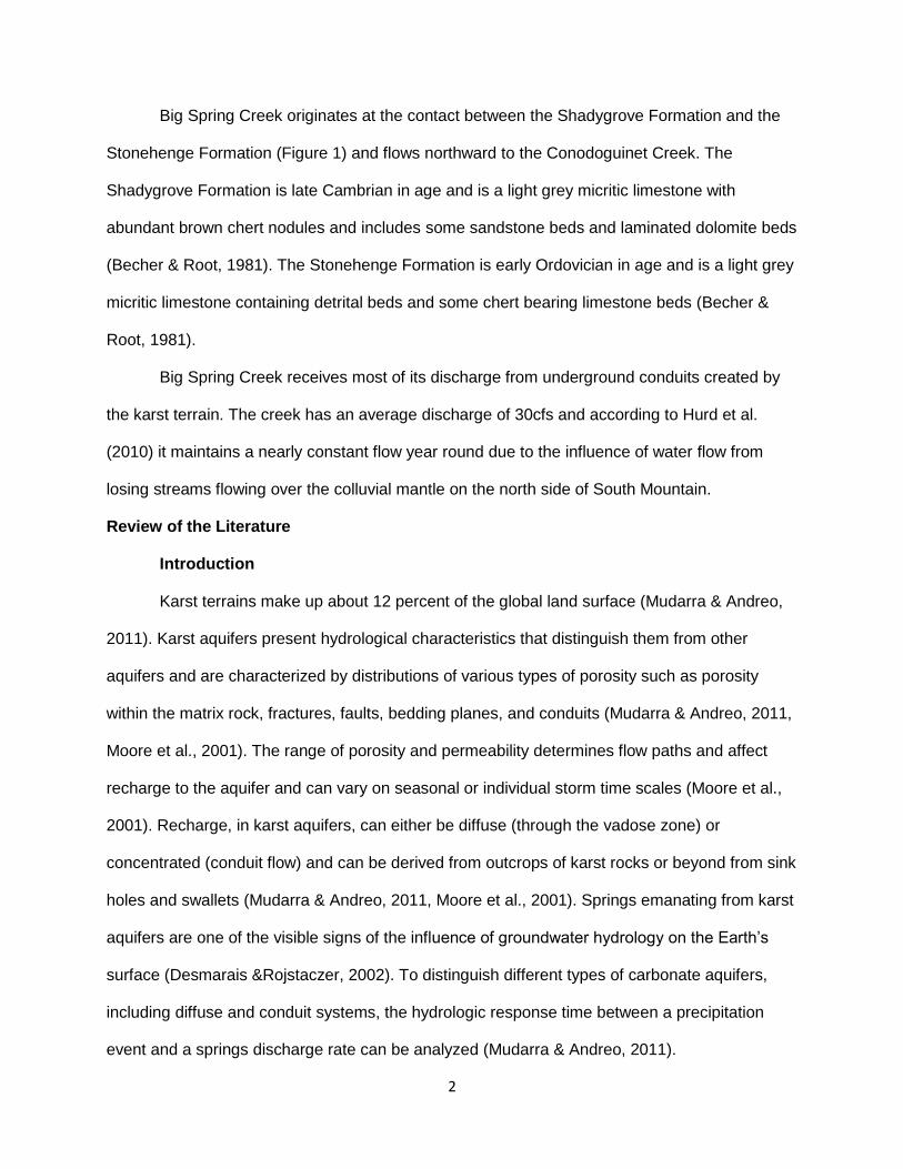
Figure 6: Hydrograph for June and July 2006, illustrating lag time
between precipitation and discharge at Big Spring Creek
during a period of surplus.
Data source: USGS and Shippensburg University
Figure 5: Illustration of average daily discharge and precipitation at
Big Spring Creek for May-July 2005 showing increased
decline in discharge rates even with large precipitation
events. Data source: USGS and Shippensburg University
0.0
10.0
20.0
30.0
40.0
50.0
60.0
0.0
0.2
0.4
0.6
0.8
1.0
1.2
5/1
/20
05
5/8
/20
05
5/1
5/2
005
5/2
2/2
005
5/2
9/2
005
6/5
/20
05
6/1
2/2
005
6/1
9/2
005
6/2
6/2
005
7/3
/20
05
7/1
0/2
005
7/1
7/2
005
7/2
4/2
005
7/3
1/2
005
Pre
cip
itat
ion
(m
m)
Dis
char
ge (
cms)
Date Discharge (cms) Precip
0.0
10.0
20.0
30.0
40.0
50.0
60.0
70.0
0.0
0.5
1.0
1.5
2.0
6/1
/20
06
6/5
/20
06
6/9
/20
06
6/1
3/2
006
6/1
7/2
006
6/2
1/2
006
6/2
5/2
006
6/2
9/2
006
7/3
/20
06
7/7
/20
06
7/1
1/2
006
7/1
5/2
006
7/1
9/2
006
7/2
3/2
006
7/2
7/2
006
7/3
1/2
006
Pre
cip
itat
ion
(m
m)
Dis
char
ge (
cms)
Date Discharge (cms) Precip
When looking at the average daily discharge and precipitation from May 1, 2005 to July
31, 2005 (Figure 5), it shows that discharge steadily declines with some small responses to
precipitation with the exception of July
15th where no response is noted. This
relationship between deficit and
lowered discharge can be seen in the
summer months of 2005, 2006, 2007,
and 2008 and on a smaller scale in
2009. This decline indicates that when
a deficit is present, and there is a high
precipitation event, water is either being
stored or used for evapotranspiration instead of flowing as runoff to Big Spring Creek. The
discharge at Big Spring Creek seems to follow the rates of surplus and deficit moisture with a
few exceptions such as the winter of 2007 where precipitation and storage are high but
discharge shows a decline.
The amount of precipitation
also has an impact on the amount of
discharge. High precipitation, during
periods of surplus, tends to lead to an
increase in the amount of discharge
after a small lag time (Figure 6). There
are some discrepancies between
precipitation and discharge: during the
spring of 2005 there is a large increase
in the amount of discharge, but little precipitation. This anomaly is not repeated even though
there are years with much higher rainfall totals. The spring of 2010, there is a similar smaller
8
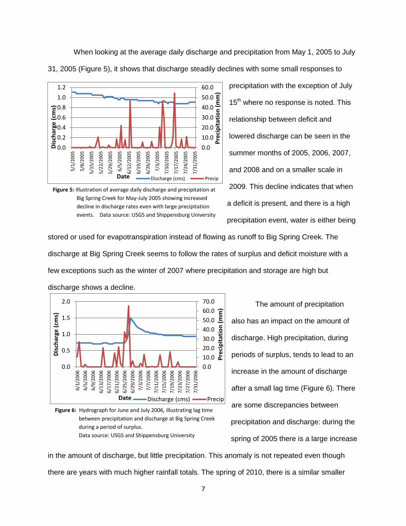
Figure 7: illustration of the relationship between Big Spring
Creeks average monthly discharge rates and
various calculations for runoff and surplus amounts
from the water budget for 2005-2010.
Data source: USGS and Shippensburg University
y = 0.0023x + 0.7585 R² = 0.1281
0.0
0.2
0.4
0.6
0.8
1.0
1.2
1.4
0.0 20.0 40.0 60.0 80.0 100.0
Dis
char
ge (
cms)
Runoff (mm)
70/30
y = 0.0028x + 0.7462 R² = 0.1147
0.0
0.2
0.4
0.6
0.8
1.0
1.2
1.4
0.0 20.0 40.0 60.0 80.0
Dis
char
ge (
cms)
Runoff (mm)
80/20
y = 0.0017x + 0.7784 R² = 0.1007
0.0
0.2
0.4
0.6
0.8
1.0
1.2
1.4
0.0 20.0 40.0 60.0 80.0 100.0
Dis
char
ge (
cms)
Runoff (mm)
60/40 increase in the amount of discharge with
no major precipitation amount. This may
indicate that there were large snowmelt
events in the spring months which
increased runoff rates with no
precipitation being recorded.
The water budget was initially
calculated with a ratio of 50/50, with 50
percent of precipitation being held in
storage for future use and 50 percent
used immediately for runoff. The
calculations for storage and runoff were
then manipulated to find the best fit for
the hydrology of Big Spring Creek. In
order to compare the average monthly
discharge and the calculated runoff from
the water budget, scatterplots were
created and the R squared value was
used to determine the strength of the
relationship between discharge and
runoff. Figure 7 indicates that the
strongest relationship between discharge and runoff occurs with a ratio of 70/30 with 70 percent
of precipitation held in storage and 30 percent available for runoff. This ratio has the highest R
squared value of 0.1281. When the water budget ratio, was adjusted to 60/40 (60% held in
storage, 40% available for runoff) the R squared value decreased to 0.1007 and when the ratio
was adjusted to 80/20 the R squared value decreased to 0.1147 between discharge and runoff.
9
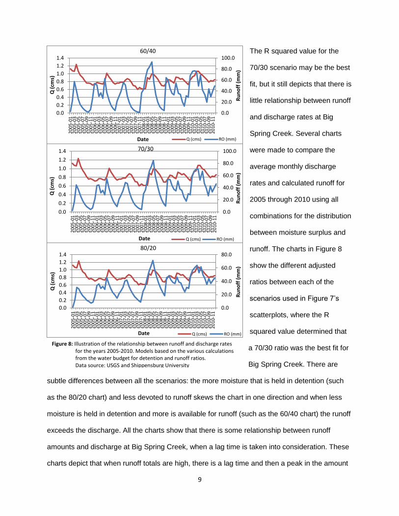
Figure 8: Illustration of the relationship between runoff and discharge rates for the years 2005-2010. Models based on the various calculations from the water budget for detention and runoff ratios. Data source: USGS and Shippensburg University
0.0
20.0
40.0
60.0
80.0
100.0
0.0
0.2
0.4
0.6
0.8
1.0
1.2
1.4
20
05-0
12
005
-03
20
05-0
52
005
-07
20
05-0
92
005
-11
20
06-0
12
006
-03
20
06-0
52
006
-07
20
06-0
92
006
-11
20
07-0
12
007
-03
20
07-0
52
007
-07
20
07-0
92
007
-11
20
08-0
12
008
-03
20
08-0
52
008
-07
20
08-0
92
008
-11
20
09-0
12
009
-03
20
09-0
52
009
-07
20
09-0
92
009
-11
20
10-0
12
010
-03
20
10-0
52
010
-07
20
10-0
92
010
-11
Ru
no
ff (
mm
)
Q (
cms)
Date
70/30
Q (cms) RO (mm)
0.0
20.0
40.0
60.0
80.0
100.0
0.0
0.2
0.4
0.6
0.8
1.0
1.2
1.4
20
05-0
12
005
-03
20
05-0
52
005
-07
20
05-0
92
005
-11
20
06-0
12
006
-03
20
06-0
52
006
-07
20
06-0
92
006
-11
20
07-0
12
007
-03
20
07-0
52
007
-07
20
07-0
92
007
-11
20
08-0
12
008
-03
20
08-0
52
008
-07
20
08-0
92
008
-11
20
09-0
12
009
-03
20
09-0
52
009
-07
20
09-0
92
009
-11
20
10-0
12
010
-03
20
10-0
52
010
-07
20
10-0
92
010
-11
Ru
no
ff (
mm
)
Q (
cms)
Date
60/40
Q (cms) RO (mm)
0.0
20.0
40.0
60.0
80.0
0.0
0.2
0.4
0.6
0.8
1.0
1.2
1.4
20
05-0
12
005
-03
20
05-0
52
005
-07
20
05-0
92
005
-11
20
06-0
12
006
-03
20
06-0
52
006
-07
20
06-0
92
006
-11
20
07-0
12
007
-03
20
07-0
52
007
-07
20
07-0
92
007
-11
20
08-0
12
008
-03
20
08-0
52
008
-07
20
08-0
92
008
-11
20
09-0
12
009
-03
20
09-0
52
009
-07
20
09-0
92
009
-11
20
10-0
12
010
-03
20
10-0
52
010
-07
20
10-0
92
010
-11
Ru
no
ff (
mm
)
Q (
cms)
Date
80/20
Q (cms) RO (mm)
The R squared value for the
70/30 scenario may be the best
fit, but it still depicts that there is
little relationship between runoff
and discharge rates at Big
Spring Creek. Several charts
were made to compare the
average monthly discharge
rates and calculated runoff for
2005 through 2010 using all
combinations for the distribution
between moisture surplus and
runoff. The charts in Figure 8
show the different adjusted
ratios between each of the
scenarios used in Figure 7’s
scatterplots, where the R
squared value determined that
a 70/30 ratio was the best fit for
Big Spring Creek. There are
subtle differences between all the scenarios: the more moisture that is held in detention (such
as the 80/20 chart) and less devoted to runoff skews the chart in one direction and when less
moisture is held in detention and more is available for runoff (such as the 60/40 chart) the runoff
exceeds the discharge. All the charts show that there is some relationship between runoff
amounts and discharge at Big Spring Creek, when a lag time is taken into consideration. These
charts depict that when runoff totals are high, there is a lag time and then a peak in the amount
10
y = 0.0043x + 0.6802 R² = 0.4774
0.0
0.2
0.4
0.6
0.8
1.0
1.2
1.4
0.0 20.0 40.0 60.0 80.0 100.0
Dis
char
ge (
cms)
Runoff (mm)
0.0
0.2
0.4
0.6
0.8
1.0
1.2
1.4
0.0
10.0
20.0
30.0
40.0
50.0
60.0
70.0
80.0
90.0
20
05-0
3
20
05-0
8
20
06-0
1
20
06-0
6
20
06-1
1
20
07-0
4
20
07-0
9
20
08-0
2
20
08-0
7
20
08-1
2
20
09-0
5
20
09-1
0
20
10-0
3
20
10-0
8
Dis
char
ge (
cms)
Ru
no
ff (
mm
)
Date RO (mm) Q (cms)
Figure 10: Relationship between calculated runoff and discharge. When
runoff is projected one month into the future and matched to
Big Springs discharge rates.
Data source: USGS and Shippensburg University
of discharge. There are exceptions where high runoff does not coincide with a peak in discharge
(such as November 2007). When calculated runoff totals are low there is a similar decline in the
amount of discharge at Big Spring. There are several instances when discharge and runoff do
not coincide. One example is October 2005, where there is an increase in discharge but runoff
remains low. This may indicate that flow is being sustained and increased from water storage.
To compensate for the lag
time between calculated runoff and
peaks in discharge rates, a
scatterplot was created where runoff
was moved forward a month to
match future discharge rates (Figure
9). By projecting runoff to a month in
the future, the R squared value is
increased from 0.1281(Figure 7) to
0.4774 (both R squared values use
the 70/30 ratio) showing that there is
more of a relationship between
discharge and runoff when runoff is
projected into the future. This can be
seen in Figure 10, where calculated
runoff amounts coincide and, in
some areas, exceed peaks in
discharge. The water budget calculation does not consider the size of the drainage basin nor
does it differentiate between rapid surface flow and slower moving groundwater flow. Figure 10
illustrates that Big Spring Creek’s discharge shows more of a response to runoff when the runoff
Figure 9: Relationship between projected calculated runoff (3/2005-
11/2010) and Big Spring Creeks discharge rates (4/2005-
12/2010). Data source: USGS and Shippensburg University
11
y = 0.3143x + 29.579 R² = 0.0004
0
10
20
30
40
50
60
0 1 2 3 4
Dis
char
ge (
cfs)
Precipitation (inches)
0
1
2
3
4
0
20
40
60
1/1
/20
05
4/1
/20
05
7/1
/20
05
10
/1/2
005
1/1
/20
06
4/1
/20
06
7/1
/20
06
10
/1/2
006
1/1
/20
07
4/1
/20
07
7/1
/20
07
10
/1/2
007
1/1
/20
08
4/1
/20
08
7/1
/20
08
10
/1/2
008
1/1
/20
09
4/1
/20
09
7/1
/20
09
10
/1/2
009
1/1
/20
10
4/1
/20
10
7/1
/20
10
10
/1/2
010
Pre
cip
itat
ion
(in
che
s)
Dis
cah
rge
(cf
s)
Date Discharge (cfs) Precip
Figure 12: Comparison between daily discharge and precipitation for 2005-2010.
Data source: USGS and Shippensburg University
is projected into the future month’s discharge. This may indicate that Big Spring’s discharge is
dominated by a more diffuse flow from moisture that is held in storage and is being slowly
released or that recharge is occurring from slower moving groundwater.
By adjusting the water budget calculations, to 70 percent water moisture held in storage
and to 30 percent of water available to runoff a more accurate depiction between discharge and
runoff was able to be made. When runoff was projected a month into the future and compared
with Big Springs discharge the relationship with runoff was visibly increased.
Analysis of daily precipitation and discharge
To show the results between average daily precipitation and average daily discharge, for
2005 to 2010, a scatterplot was created (Figure 11). The results of the scatterplot show that
when daily precipitation and discharge
are compared there is little statistical
relationship between the two. This
relationship or lack thereof, can be seen
in Figure 12 where there are a few
precipitation events that directly coincide
with increased discharge rates such as Figure 11: Scatterplot showing the relationship between daily
discharge and precipitation for 2005-2010.
Data source: USGS and Shippensburg University
12
y = -2.733x + 36.193 R² = 0.0474
0
10
20
30
40
50
60
0 0.5 1 1.5 2 2.5 3
Dis
char
ge (
cfs)
Precipitation (inches)
0
0.5
1
1.5
2
2.5
3
0
10
20
30
40
50
60
6/2
2/2
006
6/2
3/2
006
6/2
4/2
006
6/2
5/2
006
6/2
6/2
006
6/2
7/2
006
6/2
8/2
006
6/2
9/2
006
Pre
cip
itat
ion
(in
che
s)
Dis
char
ge (
cfs)
Day Q(cfs) Precip
Figure 13: Relationship between daily precipitation and discharge
during a seven day precipitation event for June 22, 2006
– June 29, 2006.
Data source: USGS and Shippensburg University
June 27, 2006 when over two and a half inches of rainfall occurred and on June 28, 2006
discharge increased to over 50cfs (average discharge is 30cfs). This shows that with large
rainfall events there is a short lag time (1 day) then a peak in discharge. When the chart is
viewed as a whole, there is little correlation between precipitation and discharge at Big Spring
Creek.
Scatterplots and graphs were used to compare, on a daily basis, two separate large
rainfall events. One of the events took place from June 22, 2006 to June 29, 2006 where 6.42
inches of rainfall occurred over the seven
day time period. The other took place
from September 26, 2010 to October 2,
2010 where 5.34 inches of rainfall
occurred over a six day time period. The
scatterplot for the 2006 rainfall shows
little relationship between the event and
discharge rates at Big Spring Creek
(Figure 13). Increases in discharge
correlate more to decreased precipitation
as shown by the trend line. When viewing
the graph of precipitation versus the
discharge at Big Spring Creek, decreased
precipitation relates to little response in
discharge. As the amount of precipitation increases, there is a lag time of a day and the
discharge rate begins to climb and at the height of the event, discharge peaks then starts
declining. This relationship is indicative that storm water flow is causing the immediate rise in
discharge but doesn’t affect the long term average discharge rates at Big Spring Creek. The
13
y = 0.0493x + 28.623 R² = 0.0024
28
28
29
29
30
30
31
31
32
0 1 2 3 4
Dis
char
ge (
cfs)
Precipitation (inches)
0
0.5
1
1.5
2
2.5
3
3.5
26
27
28
29
30
31
32
9/2
6/2
010
9/2
7/2
010
9/2
8/2
010
9/2
9/2
010
9/3
0/2
010
10
/1/2
010
Pre
cip
itat
ion
(in
che
s)
Dis
char
ge (
cfs)
Day Q(cfs) Precip
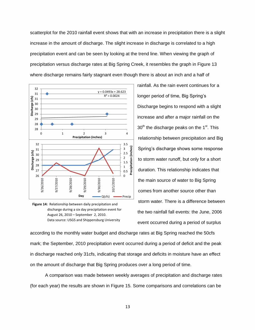
scatterplot for the 2010 rainfall event shows that with an increase in precipitation there is a slight
increase in the amount of discharge. The slight increase in discharge is correlated to a high
precipitation event and can be seen by looking at the trend line. When viewing the graph of
precipitation versus discharge rates at Big Spring Creek, it resembles the graph in Figure 13
where discharge remains fairly stagnant even though there is about an inch and a half of
rainfall. As the rain event continues for a
longer period of time, Big Spring’s
Discharge begins to respond with a slight
increase and after a major rainfall on the
30th the discharge peaks on the 1st. This
relationship between precipitation and Big
Spring’s discharge shows some response
to storm water runoff, but only for a short
duration. This relationship indicates that
the main source of water to Big Spring
comes from another source other than
storm water. There is a difference between
the two rainfall fall events: the June, 2006
event occurred during a period of surplus
according to the monthly water budget and discharge rates at Big Spring reached the 50cfs
mark; the September, 2010 precipitation event occurred during a period of deficit and the peak
in discharge reached only 31cfs, indicating that storage and deficits in moisture have an effect
on the amount of discharge that Big Spring produces over a long period of time.
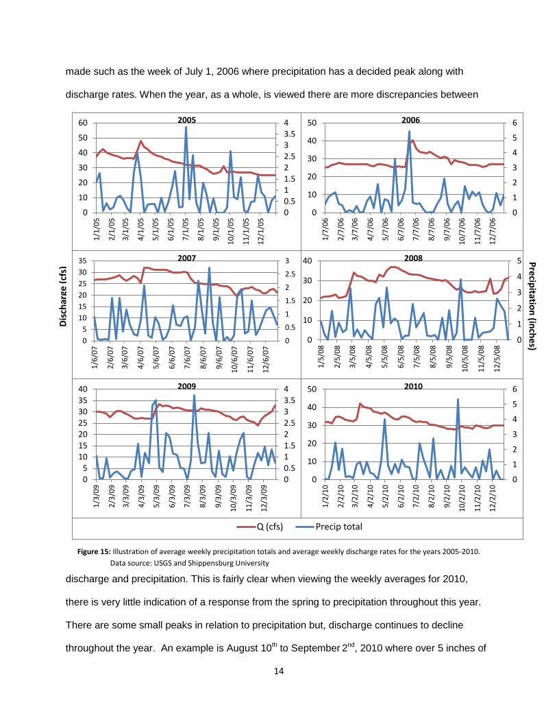
A comparison was made between weekly averages of precipitation and discharge rates
(for each year) the results are shown in Figure 15. Some comparisons and correlations can be
Figure 14: Relationship between daily precipitation and
discharge during a six day precipitation event for
August 26, 2010 – September 2, 2010.
Data source: USGS and Shippensburg University
14
0
1
2
3
4
5
6
0
10
20
30
40
50
1/7
/06
2/7
/06
3/7
/06
4/7
/06
5/7
/06
6/7
/06
7/7
/06
8/7
/06
9/7
/06
10
/7/0
6
11
/7/0
6
12
/7/0
6
2006
0
0.5
1
1.5
2
2.5
3
0
5
10
15
20
25
30
35
1/6
/07
2/6
/07
3/6
/07
4/6
/07
5/6
/07
6/6
/07
7/6
/07
8/6
/07
9/6
/07
10
/6/0
7
11
/6/0
7
12
/6/0
72007
0
1
2
3
4
5
0
10
20
30
40
1/5
/08
2/5
/08
3/5
/08
4/5
/08
5/5
/08
6/5
/08
7/5
/08
8/5
/08
9/5
/08
10
/5/0
8
11
/5/0
8
12
/5/0
8
2008
00.511.522.533.54
0
10
20
30
40
50
60
1/1
/05
2/1
/05
3/1
/05
4/1
/05
5/1
/05
6/1
/05
7/1
/05
8/1
/05
9/1
/05
10
/1/0
5
11
/1/0
5
12
/1/0
5
2005
010
050
Q (cfs) Precip total
00.511.522.533.54
05
10152025303540
1/3
/09
2/3
/09
3/3
/09
4/3
/09
5/3
/09
6/3
/09
7/3
/09
8/3
/09
9/3
/09
10
/3/0
9
11
/3/0
9
12
/3/0
9
2009
0
1
2
3
4
5
6
0
10
20
30
40
50
1/2
/10
2/2
/10
3/2
/10
4/2
/10
5/2
/10
6/2
/10
7/2
/10
8/2
/10
9/2
/10
10
/2/1
0
11
/2/1
0
12
/2/1
0
2010
made such as the week of July 1, 2006 where precipitation has a decided peak along with
discharge rates. When the year, as a whole, is viewed there are more discrepancies between
discharge and precipitation. This is fairly clear when viewing the weekly averages for 2010,
there is very little indication of a response from the spring to precipitation throughout this year.
There are some small peaks in relation to precipitation but, discharge continues to decline
throughout the year. An example is August 10th to September 2nd, 2010 where over 5 inches of
Dis
char
ge (
cfs)
Pre
cipitatio
n (in
che
s)
Figure 15: Illustration of average weekly precipitation totals and average weekly discharge rates for the years 2005-2010.
Data source: USGS and Shippensburg University
15
precipitation is recorded but there is no peak in the discharge rate. This response is probably
related to a seasonal deficit in the water budget for the year. Increased discharge in the spring
of 2010 may indicate a lag time from precipitation being held in storage, from the 2009 year, and
then released in the spring of 2010 possibly as snowmelt.
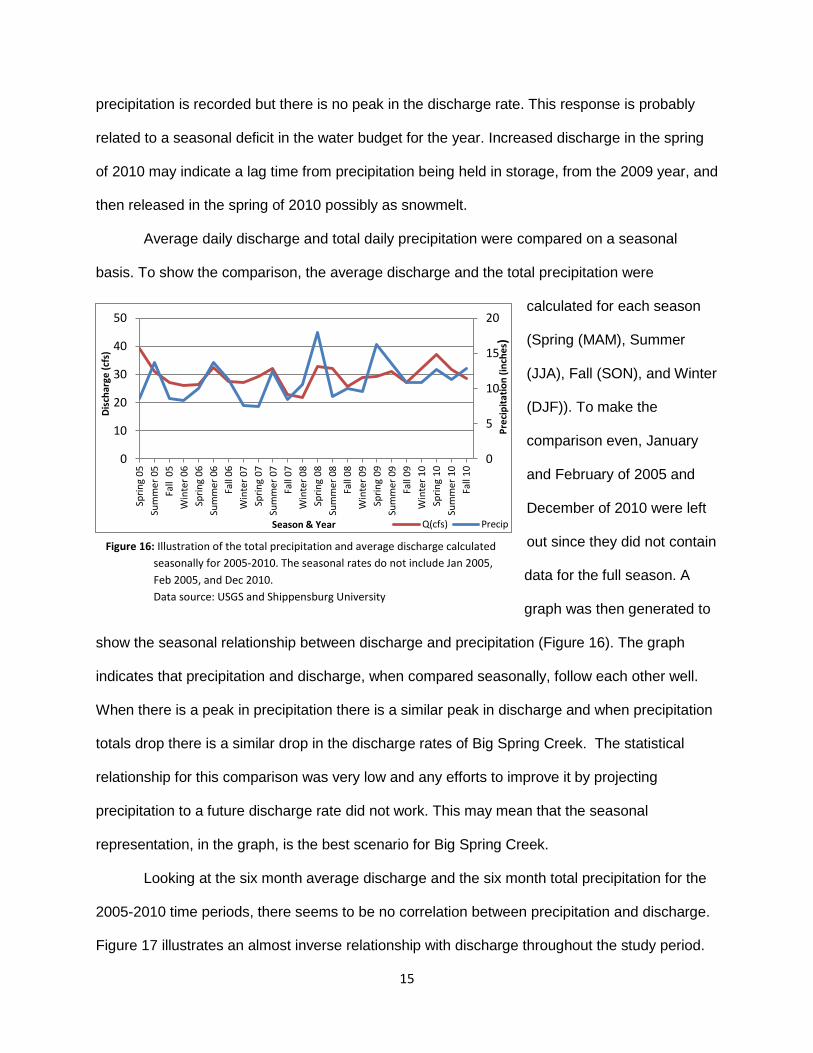
Average daily discharge and total daily precipitation were compared on a seasonal
basis. To show the comparison, the average discharge and the total precipitation were
calculated for each season
(Spring (MAM), Summer
(JJA), Fall (SON), and Winter
(DJF)). To make the
comparison even, January
and February of 2005 and
December of 2010 were left
out since they did not contain
data for the full season. A
graph was then generated to
show the seasonal relationship between discharge and precipitation (Figure 16). The graph
indicates that precipitation and discharge, when compared seasonally, follow each other well.
When there is a peak in precipitation there is a similar peak in discharge and when precipitation
totals drop there is a similar drop in the discharge rates of Big Spring Creek. The statistical
relationship for this comparison was very low and any efforts to improve it by projecting
precipitation to a future discharge rate did not work. This may mean that the seasonal
representation, in the graph, is the best scenario for Big Spring Creek.
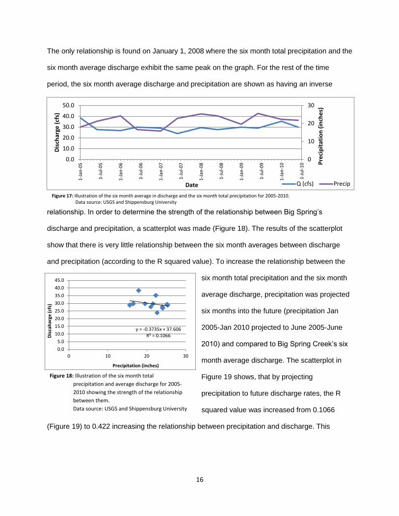
Looking at the six month average discharge and the six month total precipitation for the
2005-2010 time periods, there seems to be no correlation between precipitation and discharge.
Figure 17 illustrates an almost inverse relationship with discharge throughout the study period.
0
5
10
15
20
0
10
20
30
40
50
Spri
ng
05
Sum
mer
05
Fall
05
Win
ter
06
Spri
ng
06
Sum
mer
06
Fall
06
Win
ter
07
Spri
ng
07
Sum
mer
07
Fall
07
Win
ter
08
Spri
ng
08
Sum
mer
08
Fall
08
Win
ter
09
Spri
ng
09
Sum
mer
09
Fall
09
Win
ter
10
Spri
ng
10
Sum
mer
10
Fall
10
Pre
cip
itat
ion
(in
che
s)
Dis
char
ge (
cfs)
Season & Year Q(cfs) Precip
Figure 16: Illustration of the total precipitation and average discharge calculated
seasonally for 2005-2010. The seasonal rates do not include Jan 2005,
Feb 2005, and Dec 2010.
Data source: USGS and Shippensburg University
16
0
10
20
30
0.0
10.0
20.0
30.0
40.0
50.0
1-J
an-0
5
1-J
ul-
05
1-J
an-0
6
1-J
ul-
06
1-J
an-0
7
1-J
ul-
07
1-J
an-0
8
1-J
ul-
08
1-J
an-0
9
1-J
ul-
09
1-J
an-1
0
1-J
ul-
10 P
reci
pit
atio
n (
inch
es)
Dis
char
ge (
cfs)
Date Q (cfs) Precip
y = -0.3735x + 37.606 R² = 0.1066
0.0
5.0
10.0
15.0
20.0
25.0
30.0
35.0
40.0
45.0
0 10 20 30
Dis
cah
arge
(cf
s)
Precipitation (inches)
The only relationship is found on January 1, 2008 where the six month total precipitation and the
six month average discharge exhibit the same peak on the graph. For the rest of the time
period, the six month average discharge and precipitation are shown as having an inverse
relationship. In order to determine the strength of the relationship between Big Spring’s
discharge and precipitation, a scatterplot was made (Figure 18). The results of the scatterplot
show that there is very little relationship between the six month averages between discharge
and precipitation (according to the R squared value). To increase the relationship between the
six month total precipitation and the six month
average discharge, precipitation was projected
six months into the future (precipitation Jan
2005-Jan 2010 projected to June 2005-June
2010) and compared to Big Spring Creek’s six
month average discharge. The scatterplot in
Figure 19 shows, that by projecting
precipitation to future discharge rates, the R
squared value was increased from 0.1066
(Figure 19) to 0.422 increasing the relationship between precipitation and discharge. This
Figure 17: Illustration of the six month average in discharge and the six month total precipitation for 2005-2010. Data source: USGS and Shippensburg University
Figure 18: Illustration of the six month total
precipitation and average discharge for 2005-
2010 showing the strength of the relationship
between them.
Data source: USGS and Shippensburg University
17
0
10
20
30
40
50
60
0.0
5.0
10.0
15.0
20.0
25.0
30.0
35.0
2004 2006 2008 2010 2012
Pre
cip
itat
ion
(in
che
s)
Dis
char
ge (
cfs)
Year
Q (cfs)
Precip
Figure 21: Illustration of total yearly precipitation and average yearly discharge rates for 2005-2010. Data source: USGS and Shippensburg University
Figure 20: The average six month discharge and the six month total precipitation for 2005-2010. Precipitation was
projected six months into the future. Data source: USGS and Shippensburg University
y = 0.5147x + 17.87 R² = 0.422
0.00
5.00
10.00
15.00
20.00
25.00
30.00
35.00
40.00
0 10 20 30
Dis
cah
rge
(cf
s)
Precipitation (inches)
Figure 19: The average six month discharge and the six
month total precipitation for 2005-2010.
Precipitation was projected six months into the
future and the relationship between
precipitation and discharge shown.
Data source: USGS and Shippensburg University
0
5
10
15
20
25
30
0.00
10.00
20.00
30.00
40.00
1-J
un
-05
1-D
ec-0
5
1-J
un
-06
1-D
ec-0
6
1-J
un
-07
1-D
ec-0
7
1-J
un
-08
1-D
ec-0
8
1-J
un
-09
1-D
ec-0
9
1-J
un
-10 P
reci
pit
atio
n (
inch
es)
Dis
char
ge (
cfs)
Date Q(cfs) Precip
relationship can be seen in the graph (Figure
20) and shows that precipitation and discharge
follow each fairly well with one exception, June
1, 2008. On June 1st, there is an increase in
precipitation but, a decrease in discharge is
shown. The relationship between the average
six month discharge rate and the six month
total precipitation indicate that very little
precipitation is effectively transferred to the
spring during rainfall events and that it is held in storage and slowly released to the system at a
point in the future similar to the lag time seen with runoff only on a longer time scale.
A final comparison was made
for the total yearly precipitation
amounts and the average yearly
discharge for Big Spring Creek.
Figure 21 illustrates that comparing
yearly rates is not very helpful in
18
determining future discharge. This method might prove useful if there were a hundred years’
worth of data to compare and even then it would not provide an accurate assessment of
climate/discharge relationships on a day to day or month to month basis.
Discussion
The method that proved most useful was the constructing of a water budget. The results
of the comparison between discharge and the calculated water budget provided useful
information about the trends in flow experienced by Big Spring throughout the seasons. It was
shown that during the summer when evapotranspiration is high and a water deficit occurs, the
overall flow of Big Spring diminishes even though a high precipitation event might occur. During
periods of water surplus, high precipitation events are documented with peaks in the discharge
of Big Spring.
The surplus/runoff ratio was adjusted to 70/30 by using the R squared value as an
indicator of the relationship between the different models. By adjusting the ratio, discharge rates
were more easily matched with runoff and by projecting runoff to future discharge rates the
statistical relationship was increased and a better model was made. The water budget
calculation, for runoff, does not consider the size of the drainage basin nor does it differentiate
between rapid surface flow and slower moving groundwater flow. The results from this analysis
show that Big Spring is dominated by more diffuse flow from runoff that is slower moving instead
of faster moving overland flow. Peaks in discharge, during periods of high water surplus,
indicate that when the soil is saturated and evapotranspiration is low, the flow of water is
increased and relates to a response in Big Spring’s discharge.
The total daily precipitation and the average daily discharge rate showed that the
statistical relationship was almost nonexistent but, it proved useful in determining the amount of
lag time between an event and the increase in discharge. Using the total daily precipitation and
the average daily discharge, two major storm events were compared and illustrated that
discharge was not dependent on precipitation, but that when a long term precipitation event
19
occurred it generated a response in Big Spring’s discharge for a short duration. This information
helped determine that storm water flow created the small peaks in discharge after a precipitation
event but, that the main influence of flow to Big Spring comes from slower moving groundwater
sources.
When comparing average weekly discharge with the total weekly precipitation there
were very few relationships noted between discharge and precipitation. A seasonal comparison
was then made to show the total seasonal precipitation and the average seasonal discharge.
This comparison shows that when discharge and precipitation are viewed on a seasonal basis,
high precipitation coincides with increased discharge and little precipitation coincides with lower
discharge and that Big Spring follows seasonal variation fairly well although the statistical
relationship was not that good.
A comparison was made between the six month total precipitation and the six month
average discharge. The initial results of the comparison showed an inverse relationship
between precipitation and discharge. To increase the relationship, precipitation was projected
six months into the future and matched with discharge. By projecting precipitation, the statistical
relationship was increased and the results showed a close correlation between precipitation and
discharge. Indicating that Big Spring receives flow not just from immediate storm water events
but from precipitation that has percolated through the soil and is slowly being released back into
the system on a longer time scale.
Finally, when comparing the yearly average discharge and the total yearly precipitation
there was very little relationship shown between the two. This method proved not to be helpful
for determining a relationship between discharge and precipitation. In order for this method to
provide insight into the yearly patterns of discharge and precipitation more data would be
required to make a long term association and would still not provide insight into the daily or
monthly variations between precipitation and discharge.
20
Conclusion
Information from weather data can be used to make predictions about future discharge
rates for Big Spring Creek. Observing climatic conditions such as trends in surplus, deficit,
evapotranspiration rates, runoff (calculated from a water budget) and precipitation provide
insight into the conditions present at the time of increased or decreased discharge at Big Spring
Creek. By observing these past climate conditions and Big Spring’s responses to these
conditions, predictions about discharge can be made from the observations of climate patterns.
Appendix A
Date T(C) P (mm) PE (mm) P-PE (mm) SM (mm) DSM (mm) S (mm) AE (mm) D (mm) S avail (mm) RO (mm) Beta Q (cms)