Master production scheduling and sequencing at mixed-model assembly lines in the automotive industry

Master production scheduling and sequencingat mixed-model assembly lines in the automotiveindustry

Jan Dormer • Hans-Otto Gunther • Rico Gujjula

� Springer Science+Business Media New York 2013

Abstract The customization of final products in the automotive industry involves

a large number of optional parts and leads to a huge variety of operation times at the

various stations of the assembly line. The master production scheduling problem

(MPS) for high-variant mixed-model assembly lines is to assign the individual

customer-defined models of a basic product type to short-term production periods

while anticipating the negative impacts of an unbalanced model sequence at the

lower planning level. We propose a mathematical model formulation for the MPS

and develop heuristic solution procedures that attempt to minimize the workload

variability. Specifically, these procedures anticipate decisions on the mixed-model

sequence and the resulting work overload at stations which has to be balanced by the

assignment of utility workers. Furthermore, an integrated planning approach for

solving the MPS and the production sequencing problem is proposed.

Keywords Mixed-model assembly � Master production scheduling �Sequencing � Heuristic solution procedure

J. Dormer � H.-O. Gunther (&)

Department of Production Management, Technical University of Berlin,

H95, Strasse des 17. Juni 135, 10623 Berlin, Germany

e-mail: [email protected]

J. Dormer


R. Gujjula

Complevo GmbH, Marie-Elisabeth-Luders-Straße 1, 10625 Berlin, Germany


123

Flex Serv Manuf J

DOI 10.1007/s10696-013-9173-8

1 Introduction

In recent years, the concept of mass customization has been adopted in a large

number of industries. It aims at combining the advantages of low unit costs of mass

production processes with making products to individual unique requirements.

While mass production calls for repetitive production systems most often realized

through paced assembly lines, customization requires the use of flexible manufac-

turing equipment and highly versatile and skilled workforce. Since almost a

100 years ago Henry Ford inaugurated mass production assembly lines in the

automotive industry by introducing standard assembly tasks and interchangeable

components, automotive manufacturing systems have greatly changed. Today’s

automotive manufacture has to cope with a huge number of optional parts to fit the

automobile to the customers’ individual desires. With flexible manufacturing and

assembly systems developed over the recent decades, the challenge in the

automotive industry is to realize the huge variety of individual models by

producing them on the same mixed-model assembly line under rigid cycle time

conditions in an almost arbitrary order.

The main planning problems associated with high-variant mixed-model assembly

line production in the automotive industry are the following:

• Line balancing: Determine the configuration of the assembly line including the

number and the equipment of stations in the line, the assignment of tasks to

stations, and the takt time at which products are to be launched onto the line (cf.

Becker and Scholl 2006).

• Master production scheduling: Assign production orders for individual models

to production intervals over a short-term planning horizon of several days or

shifts.

• Production sequencing: Determine the sequence of the models (production

orders) for each production interval (cf. Gujjula et al. 2011).

• Material flow control: Ensure the timely release of parts from suppliers and the

in-time delivery of parts to the designated stations at the line (cf. Golz et al.

2012).

• Re-sequencing: Reorder the production sequence in case of disruptions, e.g. due

to unexpected part shortages (cf. Gujjula and Gunther 2009).

This paper deals with the master production scheduling (MPS) problem. Due to

the immense number of combinations resulting from the options for engines, paints,

wheels, upholstery, comfort items, technical and electronic assist systems and other

items each car can be seen as an individual object. Each of the numerous individual

options requires specific assembly tasks which have to be carried out at a line

consisting of several hundred stations under the regime of a strictly enforced cycle

time of only 1 or 2 min. Depending on the individual customer options the effective

operation time at a station shows great variations from cycle to cycle making it

extremely difficult to determine a daily product mix which smoothes out the

workload among the stations at the line. Without such workload balance there is the

risk of line stoppage and the need to employ utility workers at the most overloaded

stations.

J. Dormer et al.

123

In our investigation we consider an automotive manufacturer who applies the so-

called mixed-model sequencing (MMS) approach, i.e. develops a detailed model

sequence which seeks to reduce the assignment of utility operators at overloaded

stations and thus attempts to avoid line stoppages. We discuss implications and

present several heuristics to solve the MPS in an MMS planning environment.

Furthermore, we introduce a new multi-period sequencing approach to solve the

integrated problem of MPS and MMS. All approaches are evaluated using realistic

problem instances which mimic characteristics of typical real-life instances at

premium car manufacturers. It is shown that the proposed heuristics perform well

under realistic problem settings.

The remainder of this article is organized as follows. In the next section we

briefly review the existing literature and highlight the academic contribution of this

paper. In Sect. 3 we give a detailed explanation of the MPS problem in the

automotive industry and discuss the interdependencies between the MPS and the

subsequent sequencing problem. In Sect. 4 practical approaches for solving the MPS

are proposed. Particularly, we enhance the basic mathematical model formulation

and develop different heuristics to solve the MPS as well as the integrated problem

of MPS and MMS. In Sect. 5, a comprehensive numerical experimentation is

presented. The paper concludes with a discussion of the findings of our research.

2 Literature review

For quite a long time, short and mid-term planning problems in the automotive

industry did not receive much attention in the academic literature. Meyr (2004) was

the first to provide a comprehensive overview of supply chain planning problems

and order processing principles taking the premium segment of the German

automotive industry as an example. In their recent review Volling et al. (2012) give

a comprehensive review of the OR-related literature on capacity planning and order

processing in the automotive industry. Both Meyr (2004) and Volling et al. (2012)

point out to the strategy change in the automotive industry from built-to-stock

oriented production of standardized cars towards customized built-to-order

production. They further highlight the dependencies between the order promising

and the master production scheduling problem. More recently, Boysen et al. (2009a)

presented a hierarchical planning framework consisting of five steps: initial

configuration of the line, master scheduling, reconfiguration planning, sequencing

and re-sequencing. They also discussed the dependency of the MPS and the

subordinate sequencing problem. The MPS problem arising at an engine manufac-

turer that supplies the automotive industry is considered by Garcia-Sabater et al.

(2012) who present a two-stage planning framework for integrating operations

planning and scheduling. Their approach, however, is not directly applicable to the

final assembly of cars.

Only a limited number of papers address the master production scheduling

problem in the automotive industry (see the overview given in Table 1). In one of

the earliest papers by Hindi and Ploszajski (1994), the focus is on the selection of

orders from an order pool taking maximum consumption rates for optional parts and

Master production scheduling and sequencing

123

restrictions on the order mix imposed by the sales organization into account. Order

due dates are modelled indirectly by constraining the order selection to the oldest

orders in the pool. The authors present a binary linear model formulation and a

solution procedure based on Lagrangian relaxation. Principally, capacities can be

reflected in MPS in two ways, aggregated or detailed. While the aggregated

approach imposes limits on the short-term mix of specific product options, e.g. a sun

roof, the detailed approach considers the processing times of production orders at

each assembly station directly. In this regard the approach taken by Hindi and

Ploszajski (1994) can be considered as aggregate. Based on the work of Hindi and

Ploszajski (1994), Bolat (2003) formulates a unified cost function framework for the

order selection problem and introduces lower and upper bounds on the total

workload of the stations. Bolat proposes an exact Branch & Bound procedure as

well as a heuristic approach using a pair-wise exchange of production orders.

Ding and Tolani (2003) consider the problem of scheduling a number of model

types with given demand over a multi-period horizon. In their investigation which is

based on an industrial application, the objective is to evenly distribute the

production quantities of all models over the various time periods. The authors

present a mathematical model formulation and develop a two-phase heuristic

solution procedure. Boysen (2005) deals with multi-period MPS considering due

dates as well as part requirement constraints. The capacities of the stations in the

assembly line are modelled in an aggregate way. In a subsequent publication,

Boysen et al. (2009a) present extensions regarding capacity adjustments of the

assembly line. Finally, Volling (2009) presents a general mathematical model

formulation for the multi-period MPS problem. His model formulation integrates

the order acceptance problem which determines provisional due dates based on

customer preferences. The dynamic interaction between order promising and the

MPS problem was investigated by Volling and Spengler (2011). Based on a distinct

but interlinked mathematical model formulation for each problem the authors

propose a general framework which allows for real-time order promising and

execution of MPS based on rolling horizons. With respect to customer service,

resource levelling and inventory costs of different planning policies are bench-

marked using simulation.

Table 1 Literature overview of MPS

Author Multiple

periods

Material

requirements

Capacity

modelling

Due dates

Yes No Yes No Aggr. Det. Fixed Interval

Hindi and Ploszajski (1994) x x x x

Bolat (2003) x x x x

Ding and Tolani (2003) x x x x

Boysen (2005) x x x x

Boysen et al. (2009a) x x x x

Volling (2009) x x x x

Volling and Spengler (2011) x x x x

J. Dormer et al.

123

So far in the academic literature MPS is generally treated independently from

production sequencing and thus no comprehensive quantitative analysis of the

impact of MPS on the performance of mixed-model sequencing can be found. Since

our investigation aims at filling this gap we briefly review the relevant sequencing

concepts. As outlined in Boysen et al. (2009b) there are three basic sequencing

approaches, namely mixed-model sequencing (MMS), car sequencing (CS) and

level scheduling (LS). MMS considers each model to be assembled on the line as an

individual entity. In this approach detailed information on the customer-specific

options and related task times are required and based on this information the exact

position of the worker at each station after/before executing the assigned assembly

tasks are calculated in order to determine the work overload and the amount of

utility work caused by a specific production sequence. In contrast, CS is an

aggregated concept which employs so-called spacing constraints. These constraints

prescribe, for instance, that at most m out of n consecutively produced models may

be equipped with a specific option, e.g. a sun roof. This approach aims at

determining a feasible production sequence which does not violate the pre-defined

spacing rules. Finally, LS is an approach to support the Just-In-Time (JIT) principle

by smoothing parts usage at the assembly line.

Recently, particularly at premium car manufacturers attention has shifted from

CS and LS towards MMS, especially, as the huge number of optional parts creates a

high variability of task times which cannot be adequately handled by other

sequencing approaches. In particular, LS totally neglects processing times and thus

is becoming less important at least at premium car manufacturers. Still CS is the

dominating approach in the automotive industry. However, defining realistic

spacing rules for the entire assembly line consisting of several hundred stations and

considering all relevant product options is not easy and determining a feasible

production sequence which fulfils all the given spacing rules can become a tricky

task (cf. Golle et al. 2010 and Lesert et al. 2011). Experiences from automotive

plants show that line inefficiencies are regularly caused by improper or conflicting

spacing constraints. Therefore, in our investigation the MMS concept is pursued.

The MMS approach is based on distinct objectives which attempt to improve

labour productivity and reduce line inefficiencies. For instance, temporary work

overload at stations of the assembly line resulting from the production sequence is

minimized. Since the computational effort to determine optimal solutions for

problem instances of realistic size is prohibitive, heuristic solution procedures have

been proposed. For instance, Gujjula et al. (2011) present an efficient heuristic

based on Vogel’s approximation method for the classic transportation problem

which is able to cope with realistic assembly line conditions. An easy-implement-

able greedy solution procedure is proposed by Gujjula and Gunther (2010) which

dominates simple greedy heuristics known from literature for realistic problem

settings.

The major contribution of this paper is as follows. First, the interdependencies

between MPS and production sequencing are analyzed in detail. Second, we

propose several heuristics to solve the multi-period MPS problem which consider

detailed station loads at the assembly line in order to anticipate production

sequencing decisions based on the MMS principle. Third, a heuristic procedure to


123

solve the integrated planning problem of MPS and production sequencing is

presented. To our knowledge this kind of approach has not been detailed in

literature even though it is highly relevant for automotive assembly lines.

3 Problem description

In the automotive industry, customer orders are obtained from the company’s sales

organization. Initially, a time interval for the delivery of the car is arranged with the

customer. In times of modern mass customization, customers are able to modify

their orders in terms of individual options within acceptable lead times. However,

shortly before the intended production week, customer options are fixed and the

manufacturer determines the specific due date considering part supply constraints

and operational times of the plant. Finally, the customer orders are transferred into

production orders which specify the due date and the optional parts needed in the

assembly process (cf. Meyr 2004 and Volling et al. 2012). These specifications also

determine the individual capacity load caused by a production order at the various

stations in the line. Because of the large number of stations and production orders,

the final production sequence is usually determined through a hierarchical two-stage

planning process illustrated in Fig. 1. For the general framework of two-level

hierarchical planning systems we refer to Schneeweiß (2003). The principle idea

behind this planning approach is to divide the entire decision problem into

manageable sub-problems but to anticipate the consequences of the lower level

decisions already in the upper planning level.

As shown in Fig. 1 the MPS is located at the top level. Here decisions have to be

made on the selection of customer orders from an order bank for completion within

Master Production SchedulingTop Level

Bottom Level

Anticipated Sequencing Problem

Sequencing Problem

daily order mixTop-Down Influence

Production Sequence

Integrated Approach

Order BankCustomer Orders

Assembly Line Capacities

Material Requirements

Due Dates

Fig. 1 Hierarchical planning system

J. Dormer et al.

123

a short-term planning period. In contrast to standard MPS problems each customer

order has to be treated as an individual entity and capacity considerations arising

from the mixed-model assembly line have to be taken into account. In the simplest

case, one would consider only a single planning period, e.g. 1 day. More realistically,

the MPS is solved for a number of consecutive periods, e.g. days or shifts. At automotive

manufacturers MPS is typically carried out according to a rolling horizon regime. At

first the sales organization delivers day by day a quantum of customer orders

corresponding to the daily production volume of the plant. These customer orders

are released into the order bank which comprises the workload for a short-term

planning horizon, e.g. a week. Subsequently, through the MPS task customer orders

are assigned to daily periods and converted into production orders. This procedure is

repeated on a daily basis considering due dates up to which the ordered car has to be

produced. The orders selected for execution on the upcoming day are passed to the

detailed production sequencing module on the bottom-level. At this level the pre-

determined MPS has to be resolved in terms of a detailed production sequence at the

final assembly line. As a result, decisions of the MPS at the top-level restrict

possible decisions of the sequencing problem at the bottom level (top–downinfluence) and indirectly determine the performance of the production sequence.

Hence in order to guarantee feasible production sequences with high

performance, the MPS at the top level has to anticipate the characteristics and

capacities of the assembly line as well as the employed sequencing rules in a

thoughtful way.

Formally, the considered MPS problem consists of determining the values of

binary variables yot which indicate if production order o 2 O is assigned to period

t 2 T (yot = 1) or not (yot = 0). Constraints (1) ensure that each order is assigned to

exactly one period within the multi-period planning horizon.X

t2T

yot ¼ 1 8o 2 O ð1Þ

Given the number of production cycles C per period, production capacity in

terms of the number of orders to be produced per period is expressed by constraints

(2). It should be noted that this basic capacity constraint is formulated at an

aggregated level, since no individual cycle times of the assembly line are taken into

account.X

o2O

yot �C 8t 2 T ð2Þ

The basic model formulation is completed with an objective function c(y), which

describes the ‘‘costs’’ of a specific order-period assignment y. These ‘‘costs’’ express

the consequences of the product mix on the solution of the mixed-model sequencing

problem which is solved at the sub-ordinate planning level, i.e. the negative effects

of an unbalanced workload. The choice of c(y) and its implications for the

mathematical model are discussed in Sect. 4.

Min cðyÞ ð3Þ


123

Since the sequencing problem itself is extremely complex, it cannot be fully

integrated into the MPS. Hence we propose practical solution approaches for the

MPS which anticipate decisions on the mixed-model sequence and the resulting

work overload at stations which has to be balanced by the assignment of utility

workers.

In the final assembly of automobiles the line consists of serially arranged stations

and a conveyor belt which moves the cars through the stations with constant speed.

For practical reasons it is usually impossible to remove cars from their respective

positions on the conveyor. We assume that the takt time of the line is fixed. This

means that the distance on the line between any two subsequently launched cars is

always the same. Further, processing times are considered to be deterministic.

While processing a car, workers move downstream on the conveyor belt. After

finishing a car, they walk upstream to the next one in the sequence. We assume that

the walking time of workers from one car to the subsequent one is already included

in the operation times. Assembly line stations are closed, i.e. working on a car

cannot start before the car enters the station limits and work must be completed

before the car exits the station. If a worker reaches the downstream border of his/her

station while processing a car, some amount of work is left unfinished and has to be

compensated by so-called utility workers. In our investigation we consider work

overload and the associated utility work as the main performance indicator of

production sequencing. (It should be noted that at the MPS level we only address the

total amount of utility work and leave out the detailed scheduling and assignment of

utility workers to production cycles and specific stations in the line; cf. Gujjula and

Gunther (2009).)

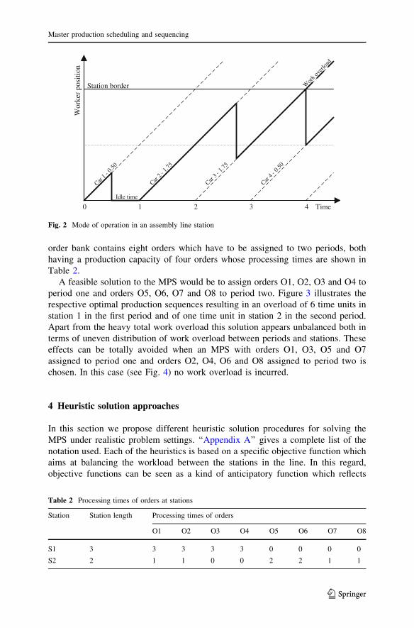
A graphical explanation of this mode of operation is given in Fig. 2 considering a

single work station whose length corresponds to twice the takt time. For convenience

the speed of the assembly line is scaled to 1. The bold line represents the position of

the worker while processing a car. At time 0 the worker starts processing car 1 for 0.5

time units and walks back to the downstream boarder of the station. Since the

processing time is less than the takt time, the worker is idle until the next car arrives at

the station. In contrast to car 1, the processing time of car 2 is greater than the takt

time. Consequently, car 3 is already within the station boundaries, when its processing

is started. Because of its processing time of 1.75 Units, car 3 cannot be finished within

the station limit and work overload of 0.5 time units occurs.

From the example of Fig. 2 it is easy to see that the solution to the sequencing

problem depends on the selection of production orders at the MPS level. To avoid

overloading work stations MPS has to take station capacities based on the available

production cycles per day, the processing times of the individual cars at each station

and the station boundaries into account. Apart from minimizing the total overload of

the work stations it is desirable to minimize the variability of work overload

throughout the production periods. The latter objective is essential because in

practice it is impossible to reconfigure the line in the short-run and to reassign tasks

from one station to another.

To further illustrate the impact of the MPS on the sequencing problem let us

consider the following elementary example of an assembly line with two stations,

S1 and S2, with a length of 3 and 2 Units, respectively. The takt time is set to 1. The

J. Dormer et al.

123

order bank contains eight orders which have to be assigned to two periods, both

having a production capacity of four orders whose processing times are shown in

Table 2.

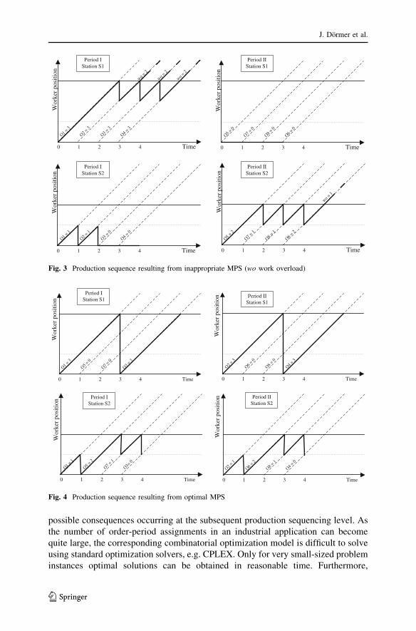
A feasible solution to the MPS would be to assign orders O1, O2, O3 and O4 to

period one and orders O5, O6, O7 and O8 to period two. Figure 3 illustrates the

respective optimal production sequences resulting in an overload of 6 time units in

station 1 in the first period and of one time unit in station 2 in the second period.

Apart from the heavy total work overload this solution appears unbalanced both in

terms of uneven distribution of work overload between periods and stations. These

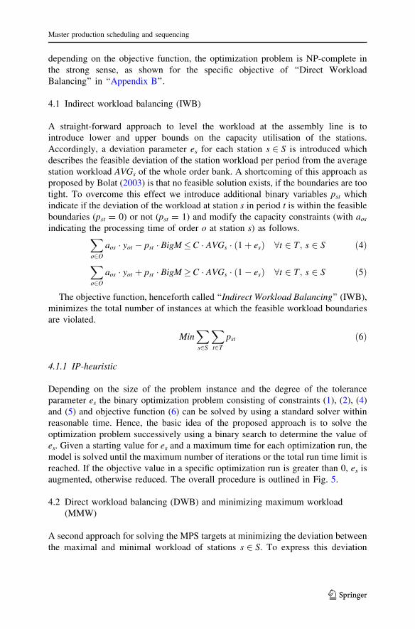
effects can be totally avoided when an MPS with orders O1, O3, O5 and O7

assigned to period one and orders O2, O4, O6 and O8 assigned to period two is

chosen. In this case (see Fig. 4) no work overload is incurred.

4 Heuristic solution approaches

In this section we propose different heuristic solution procedures for solving the

MPS under realistic problem settings. ‘‘Appendix A’’ gives a complete list of the

notation used. Each of the heuristics is based on a specific objective function which

aims at balancing the workload between the stations in the line. In this regard,

objective functions can be seen as a kind of anticipatory function which reflects

Station borderW

orke

r po

sitio

n

Car 1 -

0.50

Idle time

Wor

k ove

rload

Car 2 -

1.75

Car 3 -

1.75

Time210 3

Car 4 -

0.50

4

Fig. 2 Mode of operation in an assembly line station

Table 2 Processing times of orders at stations

Station Station length Processing times of orders

O1 O2 O3 O4 O5 O6 O7 O8

S1 3 3 3 3 3 0 0 0 0

S2 2 1 1 0 0 2 2 1 1


123

possible consequences occurring at the subsequent production sequencing level. As

the number of order-period assignments in an industrial application can become

quite large, the corresponding combinatorial optimization model is difficult to solve

using standard optimization solvers, e.g. CPLEX. Only for very small-sized problem

instances optimal solutions can be obtained in reasonable time. Furthermore,

O5 = 0

O7 = 0

O8 = 0

O6 = 0

Wor

ker

posi

tion

Time

O5 = 2

O7 = 1

O8 = 1

O6 = 2

wo = 1

Wor

ker

posi

tion

210 3 4 Time

Period IIStation S1

Wor

ker

posi

tion

Period IStation S1

O1 = 3

O2 = 3

O3 = 3

O4 = 3

wo = 2

wo = 2

wo = 2

210 3 4 Time

O1 = 1

O2 = 1

O3 = 0

O4 = 0

Wor

ker

posi

tion

210 3 4 Time

210 3 4

Period IStation S2

Period IIStation S2

Fig. 3 Production sequence resulting from inappropriate MPS (wo work overload)

Wor

ker

posi

tion Period II

Station S2

210 3 4

O2 = 3

O6 = 0

O8 = 0

O4 = 3

Time

Wor

ker

posi

tion Period II

Station S1

Wor

ker

posi

tion

O1 = 3

O5 = 0

O7 = 0

O3 = 3

O2 = 1

O6 = 2

O8 = 1

O4 = 0

210 3 4 Time

210 3 4 Time

Period IStation S1

O1 = 1

O5 = 2

O7 = 1

O3= 0

210 3 4 Time

Wor

ker

posi

tion Period I

Station S2

Fig. 4 Production sequence resulting from optimal MPS

J. Dormer et al.

123

depending on the objective function, the optimization problem is NP-complete in

the strong sense, as shown for the specific objective of ‘‘Direct Workload

Balancing’’ in ‘‘Appendix B’’.

4.1 Indirect workload balancing (IWB)

A straight-forward approach to level the workload at the assembly line is to

introduce lower and upper bounds on the capacity utilisation of the stations.

Accordingly, a deviation parameter es for each station s 2 S is introduced which

describes the feasible deviation of the station workload per period from the average

station workload AVGs of the whole order bank. A shortcoming of this approach as

proposed by Bolat (2003) is that no feasible solution exists, if the boundaries are too

tight. To overcome this effect we introduce additional binary variables pst which

indicate if the deviation of the workload at station s in period t is within the feasible

boundaries (pst = 0) or not (pst = 1) and modify the capacity constraints (with aos

indicating the processing time of order o at station s) as follows.X

o2O

aos � yot � pst � BigM�C � AVGs � ð1þ esÞ 8t 2 T; s 2 S ð4Þ

X

o2O

aos � yot þ pst � BigM�C � AVGs � ð1� esÞ 8t 2 T; s 2 S ð5Þ

The objective function, henceforth called ‘‘Indirect Workload Balancing’’ (IWB),

minimizes the total number of instances at which the feasible workload boundaries

are violated.

MinX

s2S

X

t2T

pst ð6Þ

4.1.1 IP-heuristic

Depending on the size of the problem instance and the degree of the tolerance

parameter es the binary optimization problem consisting of constraints (1), (2), (4)

and (5) and objective function (6) can be solved by using a standard solver within

reasonable time. Hence, the basic idea of the proposed approach is to solve the

optimization problem successively using a binary search to determine the value of

es. Given a starting value for es and a maximum time for each optimization run, the

model is solved until the maximum number of iterations or the total run time limit is

reached. If the objective value in a specific optimization run is greater than 0, es is

augmented, otherwise reduced. The overall procedure is outlined in Fig. 5.

4.2 Direct workload balancing (DWB) and minimizing maximum workload

(MMW)

A second approach for solving the MPS targets at minimizing the deviation between

the maximal and minimal workload of stations s 2 S. To express this deviation


123

corresponding variables zs are introduced. Constraints (7) determine the values of zs

considering each pair of periods (t1, t2).X

o2O

aos � yot1 �X

o2O

aos � yot2 � zs 8t1; t2 2 T ; s 2 S ð7Þ

The objective function, henceforth called ‘‘Direct Workload Balancing’’ (DWB),

minimizes the total amount of workload deviations over all stations.

MinX

s2S

zs ð8Þ

Alternatively, the maximum workload mw over all periods and stations can be

minimized. This strategy, called ‘‘Minimize Maximum Workload’’ (MMW), is

realized through constraints (9) and objective function (10).X

o2O

aos � yot �mw 8t 2 T ; s 2 S ð9Þ

Min mw ð10Þ

4.2.1 Two-stage heuristic for the MMW and DWB objectives

For solving complex combinatorial optimization problems a common procedure is

to first generate an initial solution and then, in the second stage, improve the initial

solution by means of a problem-specific search procedure. This two-phase solution

concept is detailed as follows.

To generate an initial solution to the optimisation problem the List-Scheduling-

Procedure (LSP) summarized in Fig. 6 is proposed. Its basic idea is to sort the given

orders in descending order of their total workload. Starting with the first order in the

list, the orders are assigned to periods one-by-one. For each station the maximum

workload over all periods

MLCs ¼ maxt2T

X

o2O

aos � yot 8s 2 S ð11Þ

Input Instance I of the Master Production Scheduling Problem, initial es, time limit per run, global time limit, maximum number of runs, es ad-aptation strategy

Output An assignment of orders to production periods1 Until global time limit or maximum number of runs is reached do2 Solve model IWB3 if objective value equals 0 then4 Save actual solution 5 Reduce es according to the adaptation strategy6 Else7 Enhance es according to the adaptation strategy8 end if-else9 end until10 return Actual solution

Fig. 5 IP heuristic

J. Dormer et al.

123

is determined in each step of the procedure. An order o is assigned to period tconsidering the production quantity constraint (2) so that the total maximum

workload over all stationsP

s2S MLCs is minimized.

To improve the initial solution the tabu search procedure outlined in Fig. 7 is

applied. This procedure is based on an exchange neighbourhood which describes the

set of schedules that can be gained from swapping order o1 with another order o2

assigned to a different period. For the neighbourhood search a Simple Swap Strategy(SSS) strategy was implemented. For each period t, it tries to swap an order o1 with

another order o2 of each succeeding period �t [ t, starting with the first period. The

objective function of the tabu search procedure is set either to the DWB or the

MMW objective function.

4.3 Process interval allocation (PIA)

The third approach for solving the MPS, called ‘‘Process Interval Allocation’’

(PIA), is based on the assumption that not only the amount of workload at a station

Input Instance I of the Master Production Scheduling Problem Output An assignment of orders to production periods

1 Generate a list L of all orders 2 Sort list L according to the total workload of the orders3 while Not all orders are assigned to a planning period do4 Choose the first order o in the list 5 Assign o to period t T that satisfies (2) so that s S sMLC is minimized6 Delete o in L7 End while8 return Assignment

Fig. 6 List scheduling procedure

Input Instance I of the Master Production Scheduling Problem, initial solu-tion y, time limit, objective function obj, ”swap-strategy”

Output An assignment X of orders to production periods1 best solution found: X y2 actual solution: Z y3 Tabu-list y4 while the time limit is not exceeded do5 Choose items o1, o2 according to the “swap-strategy”

6if Swapping o1, o2 in Z improves the objective function and the related solu-tion is not in the tabu-list then

7 swap o1 and o2 in Z8 if Z is better than X then9 X Z10 end if11 else if Z is local optimal then12 add Z to tabu-list13 Z best solution in the neighbourhood which is not in the tabu-list14 end if15 end while16 Return X

Fig. 7 Tabu search procedure


123

determines the performance of the production sequence, but also the variability of

the processing times might have an impact. Therefore, we propose a heuristic

procedure which generates an order mix for each period showing a similar

distribution of processing times as in the order bank. If for instance, p % of the

orders in the order bank has a total processing time which falls into a pre-defined

interval, e.g. representing ‘‘high’’ total processing times, then this percentage should

also be present in the daily product mix.

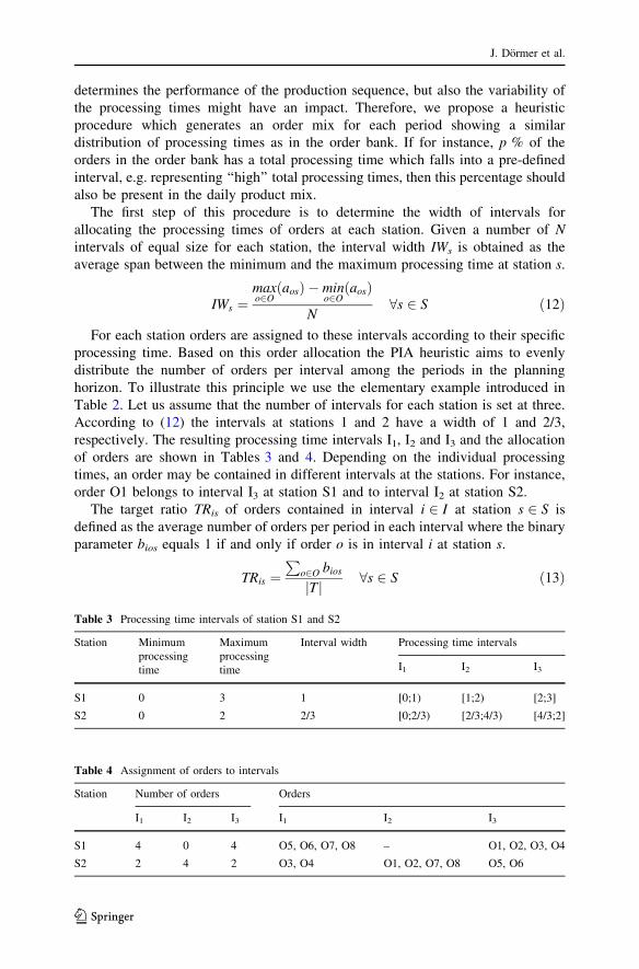
The first step of this procedure is to determine the width of intervals for

allocating the processing times of orders at each station. Given a number of Nintervals of equal size for each station, the interval width IWs is obtained as the

average span between the minimum and the maximum processing time at station s.

IWs ¼maxo2OðaosÞ � min

o2OðaosÞ

N8s 2 S ð12Þ

For each station orders are assigned to these intervals according to their specific

processing time. Based on this order allocation the PIA heuristic aims to evenly

distribute the number of orders per interval among the periods in the planning

horizon. To illustrate this principle we use the elementary example introduced in

Table 2. Let us assume that the number of intervals for each station is set at three.

According to (12) the intervals at stations 1 and 2 have a width of 1 and 2/3,

respectively. The resulting processing time intervals I1, I2 and I3 and the allocation

of orders are shown in Tables 3 and 4. Depending on the individual processing

times, an order may be contained in different intervals at the stations. For instance,

order O1 belongs to interval I3 at station S1 and to interval I2 at station S2.

The target ratio TRis of orders contained in interval i 2 I at station s 2 S is

defined as the average number of orders per period in each interval where the binary

parameter bios equals 1 if and only if order o is in interval i at station s.

TRis ¼P

o2O bios

Tj j 8s 2 S ð13Þ

Table 3 Processing time intervals of station S1 and S2

Station Minimum

processing

time

Maximum

processing

time

Interval width Processing time intervals

I1 I2 I3

S1 0 3 1 [0;1) [1;2) [2;3]

S2 0 2 2/3 [0;2/3) [2/3;4/3) [4/3;2]

Table 4 Assignment of orders to intervals

Station Number of orders Orders

I1 I2 I3 I1 I2 I3

S1 4 0 4 O5, O6, O7, O8 – O1, O2, O3, O4

S2 2 4 2 O3, O4 O1, O2, O7, O8 O5, O6

J. Dormer et al.

123

In the following constraint the variable hist is used to reflect the deviation of the

actual ratio of orders in station s and interval i from the target ratio in period t.

TRis �X

o2O

bios � yot

��

�� hist 8i 2 1. . .Nf g; s 2 S; t 2 T ð14Þ

The objective function, henceforth called ‘‘Process Interval Allocation’’ (PIA),

minimizes the total deviation of the actual from the target order mix.

MinX

i2 1...Nf g

X

s2S

X

t2T

hist ð15Þ

Additionally, the intervals at stations might be weighted according to their

importance and a corresponding weighting factor can be assigned to the variables in

the objective function. For instance, a higher weight could be assigned to critical

work stations which often show a high overload or to intervals according to their

processing time level.

4.3.1 Assignment heuristic

The problem of assigning orders to periods can be solved by use of standard solvers

for mixed-integer linear optimization problems. As an alternative we propose the

following very efficient assignment heuristic which generates the solution

iteratively. In each iteration k of the algorithm, a cost coefficient ckot is determined

for each order-period assignment. Let TRis denote the target order ratio according to

(13), gk the fraction of assigned orders after iteration k and Rk�1ist the number of

orders which have been assigned after iteration k-1 to interval i and station s in

period t. The binary parameter bios indicates if order o is in interval i at station s. Let

ais be the weight assigned to interval i and station s. In each iteration k the following

cost coefficient expresses the deviation of the current ratio of orders from the target

ratio if a yet unassigned order o is assigned to period t.

ckot ¼

X

i2 1...Nf g

X

s2S

Rk�1ist þ bios � TRis � gk

� �� ais ð16Þ

For the order-period combination showing the least value of the cost coefficient

the assignment is made. The algorithm continues until all orders are assigned. The

complete assignment heuristic is outlined in Fig. 8.

Input Instance I of the Master Production Scheduling Problem, cost function, Output An assignment of orders to production periods

1 Initialise a set of unassigned orders UO O2 Until all orders are assigned to a period do3 Calculate the assignment costs for each order UOo ∈ and each period Tt ∈4 Determine an assignment of one order to every period with minimal costs5 Fix the assignment and update UO9 end until10 return MPS solution

Fig. 8 Assignment heuristic


123

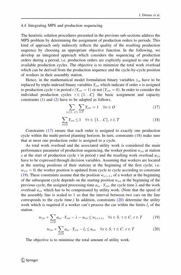
4.4 Integrating MPS and production sequencing

The heuristic solution procedures presented in the previous sub-sections address the

MPS problem by determining the assignment of production orders to periods. This

kind of approach only indirectly reflects the quality of the resulting production

sequence by choosing an appropriate objective function. In the following, we

develop an integrated approach which considers the sequencing of production

orders during a period, i.e. production orders are explicitly assigned to one of the

available production cycles. The objective is to minimize the total work overload

which can be derived from the production sequence and the cycle-by-cycle position

of workers in their assembly station.

Hence, in the mathematical model formulation binary variables yot have to be

replaced by triple-indexed binary variables Yost which indicate if order o is assigned

to production cycle s in period t Yost ¼ 1ð Þ or not Yost ¼ 0ð Þ. In order to consider the

individual production cycles s 2 1. . .Cf g the basic assignment and capacity

constraints (1) and (2) have to be adapted as follows.X

s2 1...Cf g

X

t2T

Yost ¼ 1 8o 2 O ð17Þ

X

o2O

Yost � 1 8s 2 1. . .Cf g; t 2 T ð18Þ

Constraints (17) ensure that each order is assigned to exactly one production

cycle within the multi-period planning horizon. In turn, constraints (18) make sure

that at most one production order is assigned to a cycle.

As total work overload and the associated utility work is considered the main

performance parameter of production sequencing, the worker position wsst at station

s at the start of production cycle s in period t and the resulting work overload usst

have to be expressed through decision variables. Assuming that workers are located

at the starting positions of their stations at the beginning of the first cycle, i.e.

wss1 ¼ 0, the worker position is updated from cycle to cycle according to constraint

(19). These constraints assume that the position ws;sþ1;t of a worker at the beginning

of the subsequent cycle depends on the starting position wsst at the beginning of the

previous cycle, the assigned processing time aos � Yost, the cycle time k and the work

overload usst which has to be compensated by utility work. (Note that the speed of

the assembly line is scaled to 1 so that the interval between two cars on the line

corresponds to the cycle time.) In addition, constraints (20) determine the utility

work which is required if a worker can’t process the car within the limits ls of the

station.

wsst þX

o2O

aos � Yost � k� usst�ws;sþ1;t 8s 2 S; s 2 C; t 2 T ð19Þ

wsst þX

o2O

aos � Yost � ls� usst 8s 2 S; s 2 C; t 2 T ð20Þ

The objective is to minimise the total amount of utility work.

J. Dormer et al.

123

MinX

s2S

X

s2C

X

t2T

usst ð21Þ

The corresponding mixed-integer linear optimization (MILP) model can be

solved to optimality for small-sized problem instances within reasonable time.

However, for real-life instances the use of standard solvers is impractical. Therefore,

we modify the assignment heuristic presented in the previous sub-section which is

capable of solving even excessively large problem instances with only modest

computational effort.

4.4.1 Modified assignment heuristic

For sequencing the production orders the modified assignment heuristic adopts a

priority rule based approach proposed by Gujjula and Gunther (2010), which

generates the production sequence by adding un-sequenced orders to a partial

sequence one-by-one. This approach can easily be integrated in the proposed

assignment heuristic by modifying the cost coefficient for the order-period

assignment in the following way.

According to Gujjula and Gunther (2010), the cost coefficient c0kot in iteration k of

the algorithm considers three factors, workload imbalance IBkot, utility work uk

ost and

idle time vkost which occurs if workers have to wait for the next car to enter the

station [see Eq. (22) below]. Weights c1, c2 and c3 are assigned to these factors and

can be used to parameterize the priority rule. In the assembly of premium cars,

utility work will generally be considered the primary objective by choosing a

relatively high value for c2. However, if several production orders cause the same

work overload, one might prioritize that order which yields the lowest amount of

idle time weighted with c3. A reasonably low weight should be chosen for c1 in

order to avoid so-called cherry-picking effects, i.e. assigning attractive orders to

early positions in the sequence and overlooking the ‘‘poor’’ ones. Hence, in a

practical application the range of weights should be c2 [ c3 [ c1.

c0kot ¼ c1 � IBkot þ c2 � uk

ost þ c3 � vkost ð22Þ

The first term of the objective function corresponds to the workload levelling

objective known from level scheduling (cf. Zeramdini et al. 2000). In this approach

it is desired that the workload Ak�1st assigned to station s in period t in the preceding

k-1 iterations plus the workload aos caused by the candidate order is as close as

possible to the target value which corresponds to the forward projection of the

average workload k � AVGs of that station in the order bank over k iterations. The

squared deviation of the actual and the target workload is calculated as follows.

IBkot ¼

X

s2S

k � AVGs � Ak�1st � aos

� �2 ð23Þ

In order to determine the utility work addressed in the second term of the cost

function (22) the position of workers in their respective station has to be updated

from cycle to cycle considering the continuous movement of the assembly line. Let

~wko;s;sþ1;t denote the worker position at station s at the start of production cycle sþ 1


123

in period t if candidate order o has been chosen in iteration k. In Eq. (24) ~wko;s;sþ1;t is

calculated based on the worker position ~wkosst at station s at the start of production

cycle s, the processing time aos of the candidate order, the cycle time k and the

allocated utility work ~ukosst. The latter is determined in (25) where ls denotes the

length of station s.

~wko;s;sþ1;t ¼ max 0; ~wk

osst þ aos � k� ~ukosst

� �ð24Þ

~ukosst ¼ max 0; ~wk

osst þ aos � ls� �

ð25ÞTotal utility work in iteration k for production order o is determined as the sum of

utility work occurring at the various stations of the line.

ukost ¼

X

s2S

~ukosst ð26Þ

The third term of the cost coefficient includes total idle times vkost at the assembly

line which can be derived from the station-specific idle times ~vkosst where worker

positions are obtained from (24). Respective calculations are defined in (27) and

(28).

~vkosst ¼ max 0; k� ~wk

osst � aos

� �ð27Þ

vkost ¼

X

s2S

~vkosst ð28Þ

Using the cost coefficient defined in (22) the assignment heuristic outlined in the

previous sub-section can be employed to accomplish the order-period assignments

in an iterative fashion over the multi-period planning horizon. Note that the pro-

duction sequences for a specific period directly result from the succession in which

the orders are assigned to that period. In the case post-optimization procedures are

applied, e.g. sequences are improved by tabu search, the order-period assignments

remain fixed.

5 Numerical investigation

5.1 Research questions and experimental design

In the previous section various heuristic solution procedures for solving the MPS

were presented. In the design of the heuristics we pursued different ways to

anticipate the consequences of the daily order mix at the subordinate planning level

of production sequencing. As mentioned above minimum total work overload and

minimum variation of work overload are considered as the key performance

parameters. A comprehensive numerical study was conducted in order to answer the

following research questions.

• How do the different heuristic solution procedures perform in terms of total

work overload and variation of work overload occurring at the subsequent

production sequencing level?

J. Dormer et al.

123

• Is it practical to solve the MPS and the sequencing problem by use of an

integrated approach?

• How are total work overload and variability of work overload affected by an

increased variability of processing times?

To evaluate the proposed heuristic approaches for practical application, sixteen

different scenarios inspired by observations from real assembly lines of premium

car manufacturers were generated for the numerical test. Each scenario can be

classified by the size of the corresponding problem instances (small, medium, large,

very large) and by the variability of processing times at the stations (base, low,

medium and high). The generation of scenarios follows that one of Gujjula and

Gunther (2010). Throughout the experiments the planning horizon was set as 5

periods. The problem size is characterized by the number of stations and the size of

the order bank. For instance, small scenarios comprise 50 stations and 500 orders.

These figures are doubled for every higher problem size. Capacity utilization rate at

each station is set at 95 % throughout. A summary of the problem size is given in

Table 5. At each station s four different processing times pt1s � pt2

s � 1� pt3s � pt4

s

were randomly generated from a uniform distribution with intervals given in

Table 6. Note that the cycle time is scaled to 1.

In our investigation we consider four classes of production orders depending on

the degree of optional equipment that a customer may order: simple, standard,

premium and luxury cars which differ by the processing times at the various

stations. The distribution of processing times for each order class at a station and the

associated demand rate are given in Table 7. For instance, each simple car

(production order) takes the lowest processing time pt1 at 50 %, the second-lowest

processing time pt2 at 25 % and the third-lowest processing time pt3 at 25 % of all

stations, respectively. However, the choice of these stations can be different for each

individual car. With this conception, there are usually no two cars which share the

same processing times for all stations.

The generation process of the data is as follows. At first, processing times are

generated and cars are assigned to these times in accordance with the given

distributions. Afterwards, the processing times are scaled such that an average

processing time of 0.95 time units for each station is met. At last, the length of the

stations is set as ls ¼ pt4� �

.

Since the performance of the MPS heuristics depends on the solution to the

production sequencing problem, we had to implement a reasonable and efficient

method to generate the production sequence period-by-period based on the obtained

MPS solutions. For this purpose, the sequencing algorithm of Gujjula and Gunther

Table 5 Problem sizes

Size of problem instances

Small Medium Large Very large

No. of orders 500 1,000 2,000 4,000

No. of stations 50 100 200 400


123

(2010) is applied. This algorithm explained in Sect. 4.4 generates a production

sequence one-by-one using a priority rule. The generated solution is improved by

means of a tabu search procedure, which is based on a pair-wise exchange of orders.

If the production sequence cannot be improved by swapping two orders, the current

solution is considered locally optimal and this solution is stored in a tabu list. Then

the procedure continues with the best solution in the neighbourhood that is not in the

tabu list.

It should be noted that from the academic literature no algorithms are available

which solve the joint optimization problem of MPS and order sequencing except for

unrealistically small problem instances. Therefore, we deem it reasonable to base

our numerical evaluation on a heuristic benchmark and on the total workload per

station as a proxy criterion.

Four different heuristic procedures presented in the previous section are included

in the numerical evaluation, namely indirect workload balancing (IWB) of Sect. 4.1,

direct workload balancing (DWB) and minimizing maximum workload (MMW) of

Sect. 4.2, process interval allocation (PIA) of Sect. 4.3 and the approach of

integrating MPS and production sequencing (INT) as outlined in Sect. 4.4. In

addition, a benchmark solution is determined by applying the sequencing algorithm

of Gujjula and Gunther (2010) to the entire set of production orders contained in the

order bank. The resulting production sequence is then split into sub-sequences

corresponding to the period structure of the MPS. In the presentation of the

numerical results this complete sequencing approach is labelled SEQ.

Parameter settings for the various heuristics have been made as follows. In a pre-

test different strategies for adapting the es parameter used in the IP-heuristic as part

of the IWB approach were evaluated. The best performance was achieved with

equal values of the parameter for all stations. Setting initial values of 0.1 the value

of es was enhanced according to the logic of binary search in case the objective

Table 6 Intervals of processing times and resulting variability classes

Processing time Variability class

Base Low Medium High

pt1s ; pt2

s[0, 1] [0, 1] [0, 1] [0, 1]

pt3s ; pt4

s[1, 1.5] [1, 2] [1, 3] [1, 5]

Table 7 Order classes and distribution of processing times

Order class Processing time Demand rate (%)

pt1 (%) pt2 (%) pt3 (%) pt4 (%)

Basic 50 25 25 – 33

Standard 25 50 25 – 33

Premium – 25 50 25 17

Luxury – 25 25 50 17

J. Dormer et al.

123

function value was greater than 0 and reduced otherwise. Time limits for the IP-

Heuristic (see Fig. 5) and the tabu search procedure (see Fig. 7) depending on the

size of the problem instances are given in Table 8. For solving the IP model time

limits for the tabu search heuristic associated with the integrated MPS and the

production sequencing approach of Sect. 4.4 were quadrupled in comparison to

those given in Table 8, e.g. 1,440 s for the very large scenario. For the SEQ

heuristic the same time limits are set as per period of the MPS, e.g. 7,200 s for the

very large scenario.

In the cost function (16) of the PIA heuristic outlined in Sect. 4.3 weights ais for

interval i at a station s were defined as the distance of the centre of the interval from

the average of the processing times of orders at station s. This setting is reasonable

since a large distance will most likely have a stronger impact on the sequencing

performance compared to a case of a small deviation. In a computational pre-study

(not presented in this paper) the impact of the numbers of intervals was examined.

Five intervals turned out to produce the best results. The integrated approach

outlined in Sect. 4.4 uses weights c1, c2 and c3 for the components of the cost

function (22). We normalized c1 at 1 and determined the values of c2 and c3 in a

computational pre-study. The resulting values of the weighting factors are given in

Table 9.

For each of the 16 scenarios 10 problem instances were randomly generated. All

tests were carried out on a PC with an Intel Xeon processor clocked at 2.66 GHz.

For solving the IP model of Sect. 4.1 CPLEX 12.1 was used as standard

optimization software.

5.2 Numerical results

The results of the numerical experiments for the 16 investigated scenarios are

summarized in Tables 10, 11, 12, 13. Each table refers to a specific problem size

scenario and contains the results for the various variability classes defined for the

Table 8 Time limits (s) for MPS heuristics

Procedure Size of problem instances


Tabu search 45 90 180 360

IP heuristic (total) 45 90 180 360

IP heuristic (per run) 15 30 60 120

Table 9 Settings of c2 and c3 (c1 = 1)

Weighting factor Size of problem instances


c2 20 29 46 78

c3 11 16 28 51


123

processing times at the stations of the line. Entries indicate average values over 10

replications. In the left part of the tables total work overload per station is shown.

The right part contains the standard deviation of the work overload at the stations.

Run times are given in seconds and include the construction and the improvement

phase of the heuristics.

From analyzing the numerical results of Tables 10, 11, 12, 13 several

observations can be made.

• First, the IWB heuristic of Sect. 4.1 is dominated in all of the 16 scenarios by the

other heuristics both in terms of total work overload per station and the

variability (standard deviation) of the work overload.

• Second, comparing the related DWB and MMW heuristics of Sect. 4.2 they turn

out to perform almost equivalently for all scenarios regarding total work

overload per station. However, the standard deviation of the work overload at

stations shows lower values for the DWB heuristic. Hence, this variant of the

heuristic should be preferred to its counterpart.

• Third, the PIA heuristic performs equally well compared to DWB in terms of

total work overload per station. However, particularly for the large and the very

large problem instances (see Tables 12 and 13) PIA shows a considerably lower

Table 10 Test results for small-sized instances

Heuristic Run time (s) Total work overload per station Standard deviation of work overload

Variability class Variability class

Base Low Medium High Base Low Medium High

IWB 45 9.2 9.9 14.1 18.1 62.7 69.4 107.2 156.5

DWB 45 7.5 7.8 11.2 14.1 3.6 4.4 5.6 8.9

MMW 45 7.7 8.0 11.4 14.6 5.8 5.6 6.2 11.9

PIA 1 7.5 7.9 11.4 14.3 4.1 5.6 7.0 10.8

INT \1 6.4 6.7 10.0 13.0 3.9 4.1 6.0 11.1

SEQ 900 6.5 7.0 10.3 13.3 22.0 23.3 29.2 35.8

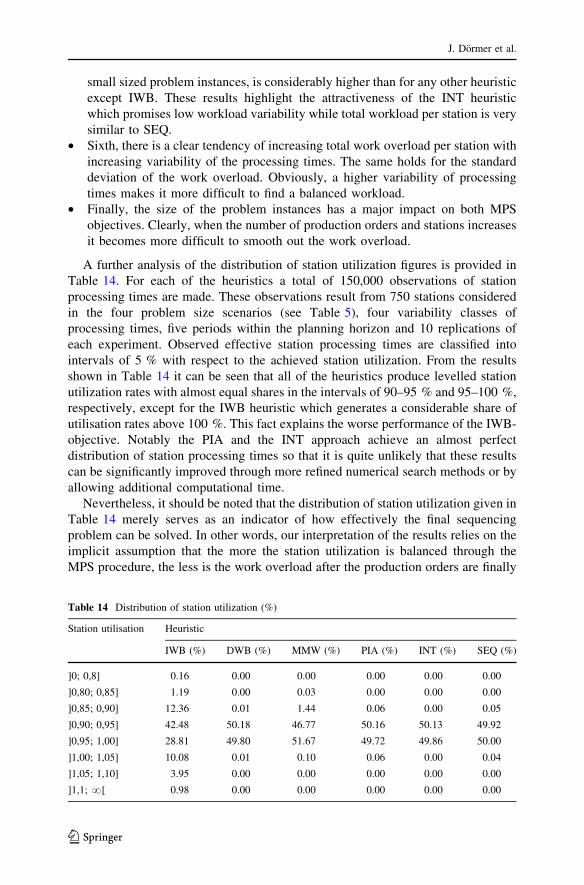
Table 11 Test results for medium-sized instances




IWB 90 24.3 27.6 35.7 42.6 212.8 287.7 408.5 477.1

DWB 90 22.1 24.8 31.6 38.1 9.8 12.8 17.7 20.6

MMW 90 22.6 25.2 32.1 38.9 24.5 28.1 29.8 43.1

PIA 7 22.1 24.8 31.6 38.1 11.1 11.4 16.3 22.8

INT 3 20.2 22.6 29.6 35.9 9.9 10.4 15.3 22.6

SEQ 1,805 19.7 22.2 29.0 35.6 90.1 110.9 130.4 141.8

J. Dormer et al.

123

standard deviation of the work overload. In addition runtimes of PIA are lower

than for DWB except for the very large problem instances. Since in each

iteration of the algorithm the cost coefficient (16) with all its terms has to be

recalculated for each of the yet unassigned orders, the corresponding compu-

tational demand grows exponentially from 1 s for small to 486 s for very large

problem instances. But still run times for the PIA heuristic are acceptable

considering the nature of the MPS problem. In conclusion, for practical

application priority should be given to PIA over DWB.

• Fourth, for all 16 test scenarios the INT heuristic outperforms PIA as the so far

best heuristic in terms of total work overload per station and for 15 out of 16

scenarios also with respect to the variability of the work overload. It is

remarkable that this superior performance is achieved at the lowest run times of

all of the tested heuristics. Notably INT not only solves the MPS but also

generates a production sequence for each planning period of the MPS.

• The fifth observation relates to the SEQ heuristic which is merely used as a

benchmark. It requires excessive run times particularly for the large and very

large sized problem instances. Nevertheless its performance in terms of total

work overload per station is only slightly better than for the INT heuristic while

at the same time the standard deviation of the work overload, except for the

Table 12 Test results for large-sized instances




IWB 181 55.7 65.5 80.7 101.1 570.3 727.8 887.7 1,270.4

DWB 181 53.6 62.8 77.4 96.6 42.0 49.1 61.7 78.8

MMW 180 54.2 63.5 78.4 97.9 107.1 115.4 124.0 169.6

PIA 61 53.7 62.9 77.5 96.7 21.3 31.1 33.1 42.3

INT 26 50.0 59.0 73.8 93.0 18.5 18.4 28.9 49.1

SEQ 3,656 49.1 57.9 72.4 91.8 334.2 419.8 506.7 560.7

Table 13 Test results for very large-sized instances




IWB 360 132.0 153.1 189.5 236.5 4,467.7 5,781.2 7,967.1 10,827.0

DWB 366 124.0 142.4 174.4 217.6 78.3 116.0 148.7 164.0

MMW 366 124.6 143.1 175.3 219.1 354.1 353.7 393.2 580.6

PIA 486 123.9 142.3 174.4 217.8 45.0 56.0 73.0 106.5

INT 191 118.1 135.8 167.5 210.3 40.6 39.6 62.9 92.3

SEQ 7,681 115.2 132.9 163.5 204.5 1,214.1 1,536.4 1,845.2 2,013.2


123

small sized problem instances, is considerably higher than for any other heuristic

except IWB. These results highlight the attractiveness of the INT heuristic

which promises low workload variability while total workload per station is very

similar to SEQ.

• Sixth, there is a clear tendency of increasing total work overload per station with

increasing variability of the processing times. The same holds for the standard

deviation of the work overload. Obviously, a higher variability of processing

times makes it more difficult to find a balanced workload.

• Finally, the size of the problem instances has a major impact on both MPS

objectives. Clearly, when the number of production orders and stations increases

it becomes more difficult to smooth out the work overload.

A further analysis of the distribution of station utilization figures is provided in

Table 14. For each of the heuristics a total of 150,000 observations of station

processing times are made. These observations result from 750 stations considered

in the four problem size scenarios (see Table 5), four variability classes of

processing times, five periods within the planning horizon and 10 replications of

each experiment. Observed effective station processing times are classified into

intervals of 5 % with respect to the achieved station utilization. From the results

shown in Table 14 it can be seen that all of the heuristics produce levelled station

utilization rates with almost equal shares in the intervals of 90–95 % and 95–100 %,

respectively, except for the IWB heuristic which generates a considerable share of

utilisation rates above 100 %. This fact explains the worse performance of the IWB-

objective. Notably the PIA and the INT approach achieve an almost perfect

distribution of station processing times so that it is quite unlikely that these results

can be significantly improved through more refined numerical search methods or by

allowing additional computational time.

Nevertheless, it should be noted that the distribution of station utilization given in

Table 14 merely serves as an indicator of how effectively the final sequencing

problem can be solved. In other words, our interpretation of the results relies on the

implicit assumption that the more the station utilization is balanced through the

MPS procedure, the less is the work overload after the production orders are finally

Table 14 Distribution of station utilization (%)

Station utilisation Heuristic

IWB (%) DWB (%) MMW (%) PIA (%) INT (%) SEQ (%)

]0; 0,8] 0.16 0.00 0.00 0.00 0.00 0.00

]0,80; 0,85] 1.19 0.00 0.03 0.00 0.00 0.00

]0,85; 0,90] 12.36 0.01 1.44 0.06 0.00 0.05

]0,90; 0,95] 42.48 50.18 46.77 50.16 50.13 49.92

]0,95; 1,00] 28.81 49.80 51.67 49.72 49.86 50.00

]1,00; 1,05] 10.08 0.01 0.10 0.06 0.00 0.04

]1,05; 1,10] 3.95 0.00 0.00 0.00 0.00 0.00

]1,1; ?[ 0.98 0.00 0.00 0.00 0.00 0.00

J. Dormer et al.

123

sequenced. However, in the absence of adequate solution algorithms for the

combined MPS and sequencing problem, there is no other choice than to follow the

divide and conquer principle, i.e. to apply a hierarchical planning approach.

Certainly, more advanced sequencing procedures, which provide an optimal

solution, would be the first choice for benchmarking the obtained MPS solutions.

But, exact sequencing procedures which are able to solve realistic problem instances

are not yet available.

6 Conclusions

Master production scheduling (MPS) is a problem class that has been investigated in

the production and operations management literature since a number of decades.

Particularly, in the Operations Research literature product mix optimization

represents one of the classic applications. Nevertheless, MPS in the automotive

industry has received only little attention so far despite the huge economic

importance of this industry sector. Contrary to conventional MPS, in automotive

production each product unit (customer order) must be considered as an individual

entity which naturally leads to complex combinatorial optimization problems. The

huge variety of optional parts and respective processing times further contributes to

the complexity of the optimization problem, especially in the production of

premium cars.

The investigation presented in this paper has been inspired by real-life problems

from the German automotive industry. Efficient and effective heuristic solution

procedures have been developed which particularly address the interface between

MPS and the subsequent production sequencing level at high-variant mixed model

assembly lines. To the best of our knowledge, these heuristics represent the first

efficient solution procedures for multi-period MPS taking the requirements of

mixed-model sequencing into account.

In the considered two-stage hierarchical planning system the performance of the

production system is determined through the final production sequences which are

constrained by the MPS at the upper level. Therefore, anticipation of the production

sequencing performance was a major concern in the design of the MPS heuristics. In

addition, an integrated planning approach (INT) which generates production

sequences for each of the planning periods was proposed.

In a comprehensive computational study, the performance of the developed

heuristics was investigated. Minimization of work overload at the stations causing

the assignment of utility workers in bottleneck situations and reduced variability of

station utilization enabling more efficient deployment of personnel were considered

as the main objectives. From the proposed MPS heuristics the integrated approach

performed superior compared to the other heuristics both in terms of the main

objectives as well as with respect to computational times.

For practical application, additional aspects might be relevant which can be

easily integrated into the presented MPS heuristics. For instance, flexible time

windows instead of crisp due dates for customer orders or levelling of part supply

in terms of minimal and/or maximal consumption rates for crucial parts and


123

sub-assemblies could be considered (cf. Boysen et al. 2009c, 2010). For further

research, it would be worth to enhance the presented planning approaches by

integrating these additional aspects and to balance off the advantage of smooth

station workload and levelled part supply.

Appendix A

Notation

Sets

O The set of orders

S The set of stations at the assembly line

T The set of planning periods

i ¼ 1. . .Nf g The intervals of processing times in the PIA heuristic

s ¼ 1. . .Cf g The set of production cycles

Parameters

aos Processing time of order o 2 O at station s 2 S

Ak�1st

Workload assigned to station s in Period t until iteration k-1

AVGs ¼P

o2Oaos

Oj jAverage workload of station s 2 S in the order bank

bios Binary parameter indicating if order o is in interval i at station s

BigM A sufficiently large number

C Number of production cycles per period

ckot; c0kot

Cost of assigning order o to period t in iteration k

es Feasible deviation from the average workload in station s 2 S

gk Fraction of assigned orders after iteration k

IBkot

Workload imbalance caused by order o in period t in iteration k

IWs Interval width of processing times at station s 2 S

ls Length of station s 2 S

N The number of processing time intervals per station and period

Rkist

Ratio of orders which have been assigned after iteration k to interval i and station s in

period t

TRis Target ratio of orders contained in interval i at station s

ukoss Total utility work of order o in production cycle s in period t in iteration k

~ukosst

Utility work at station s in production cycle s in period t if candidate order o has been

chosen in iteration k

vkoss Total idle time of order o in production cycle s in period t in iteration k

~vkosst

Idle time at station s in production cycle s in period t if candidate order o has been

chosen in iteration k

~wkosst

Worker position at station s at the start of production cycle s in period t if candidate

order o has been chosen in iteration k

ais Weight assigned to interval i and station s

c1, c2, c3 Weights assigned to terms of the cost coefficient

k Cycle time

J. Dormer et al.

123

Appendix B: Proof of NP completeness

In the following it is shown that the MPS with the DWB objective (MPS-D-DWB)

is NP-complete in the strong sense by reducing it to the well known 3-partition

problem.

Given a number B, the decision problem related to the MPS (MPS-D) with an

objective function z is to answer the following question:

Exists a feasible schedule x with an objective value zðxÞ�B?

Since a given schedule can be evaluated in polynomial time, MPS-D belongs to

NP.

The 3-partition can be formulated as follows. Let A ¼ a1; . . .; a3mf g be a set of

3m positive integers. The problem is to determine m disjoint subsets, S1; . . .; Sm,

each containing exactly 3 elements and with an equal weight:P

ai2S1ai ¼ . . . ¼P

ai2Smai.

The solution is yes if such a partition exists and no otherwise.

To reduce the MPS to the 3-partition problem it is to be proofed that an instance

of the MPS can be linearly transformed into an instance of the 3-partition problem

and if and only if the answer to the question of the MPS-D is yes the answer to the

corresponding 3-partition problem is yes, as well.

For an instance of the 3-partition problem generate an instance of the MPS-

D-DWB problem with an assembly line consisting of one single station, an order oi

for every integer ai with a processing time of a1 time units, m periods with a

capacity of 3 Units and set B equal to 0. Obviously, this transformation is linear.

Given a feasible schedule of the MPS-D-DWB the subsets S1. . .Sm can easily be

Appendix continued

Variables

hist � 0 Continuous variable which represents the deviation of the actual ratio of orders in station sand interval i from the target ratio in period t

mw� 0 Continuous variable which represents the maximum workload over all stations and

periods

pst 2 0; 1f g Binary variable which is set to 1 if the workload at station s in period t exceeds the

feasible boundaries

usst � 0 Continuous variable which represents the work overload at station s in production cycle sin period t

wsst � 0 Continuous variable which represents the worker position at station s at the start of

production cycle s in period t

yot 2 0; 1f g Binary variable which is set to 1 if and only if order o is assigned to period t

Yost 2 0; 1f g Binary variable which is set to 1 if and only if order o is assigned to cycle s in period t

MLCs� 0 Continuous variable which represents the maximum workload of station s over all periods

zs� 0 Continuous variable which represents the gap between the maximal and minimal

workload station s


123

generated by identifying every set with a period and assigning the numbers

represented by the respective orders. If the answer to the MPS-D is yes, every period

has an equal workload. Consequently, the answer to the respective 3-partition

problem is yes. Conversely, if a 3-partition exists, the subsets define a feasible

solution to the MPS-D-DWB problem. Hence, the MPS-D-DWB problem is as

complex as the 3-partition problem which is NP complete in the strong sense (cf.

Garey and Johnson 1979).

The preceding proof can easily be adopted according to the IWB, MMW and PIA

objectives of the MPS.

References

Becker C, Scholl A (2006) A survey on problems and methods in generalized assembly line balancing.

Eur J Oper Res 168(3):694–715

Bolat A (2003) A mathematical model for selecting mixed models with due dates. Int J Prod Res

41(5):897–918

Boysen N (2005) Variantenfließfertigung. Gabler, Wiesbaden (in German)

Boysen N, Fliedner M, Scholl A (2009a) Production planning of mixed model assembly lines: overview

and extensions. Prod Plann Control 20(5):455–471

Boysen N, Fliedner M, Scholl A (2009b) Sequencing mixed-model assembly lines: survey, classification

and model critique. Eur J Oper Res 192(2):349–373

Boysen N, Fliedner M, Scholl A (2009c) Level scheduling for batched JIT supply. Flex Serv Manuf

21(1–2):31–50

Boysen N, Fliedner M, Scholl A (2010) Level scheduling under limited resequencing flexibility. Flex

Serv Manuf 22(3–4):236–257

Ding FY, Tolani R (2003) Production planning to support mixed-model assembly. Comput Ind Eng

45(3):375–392

Garcia-Sabater J-P, Maheut J, Garcia-Sabater JJ (2012) A two-stage sequential planning scheme for

integrated operations planning and scheduling system using MILP: the case of an engine assembler.

Flex Serv Manuf 24(2):171–209

Garey MR, Johnson DS (1979) Computers and intractability: a guide to the theory of NP-completeness.

W.H. Freeman & Co, New York

Golle U, Boysen N, Rothlauf F (2010) Analysis and design of sequencing rules for car sequencing. Eur J

Oper Res 206(3):579–585

Golz J, Gujjula R, Gunther H-O, Rinderer S, Ziegler M (2012) Part feeding at high-variant mixed-model

assembly lines. Flex Serv Manuf 24(2):119–141

Gujjula R, Gunther H-O (2009) Scheduling utility workers at mixed-model assembly lines. In:

Proceedings of the 2009 IEEE international conference on industrial engineering and engineering

management. Sun H, Jiao R and Xie M (eds), IEEE, Singapore 2009, pp. 1092–1096

Gujjula, R., Gunther, H.-O. (2010), An efficient heuristic to sequence mixed-model assembly lines. In:

Proceedings of the 2010 IEEE international conference on industrial engineering and engineering

management. Lian Z, Wu Z, Min X, Jiao R (eds). IEEE, Singapore 2010, pp 1209–1209

Gujjula R, Werk S, Gunther H-O (2011) A heuristic based on Vogel’s approximation method for

sequencing mixed-model assembly lines. Int J Prod Res 49(21):6451–6468

Hindi KS, Ploszajski G (1994) Formulation and solution of a selection and sequencing problem in car

manufacture. Comput Ind Eng 26(1):203–211

Lesert A, Alpan G, Frein Y, Noire S (2011) Definition of spacing constraints for the car sequencing

problem. Int J Prod Res 49(2):963–994

Meyr H (2004) Supply chain planning in the German automotive industry. OR Spectrum 26(4):447–470

Schneeweiß C (2003) Distributed decision making, 2nd edn. Springer, Heidelberg

Volling T (2009) Auftragsbezogene Planung bei variantenreicher Serienproduktion. Gabler, Wiesbaden

(in German)

J. Dormer et al.

123

Volling T, Spengler T (2011) Modelling and simulation of order-driven planning policies in built-to-order

automobile production. Int J Prod Econ 131(1):183–193

Volling T, Matzke A, Grunewald M, Spengler TS (2012) Planning of capacities and orders in build-to-

order automobile production: a review. Eur J Oper Res. to appear (available online: doi:10.1016/

j.ejor.2012.07.034)

Zeramdini W, Aigbedo H, Monden Y (2000) Bicriteria sequencing for just-in-time mixed-model

assembly lines. Int J Prod Res 38(15):451–3470

Author Biographies

Jan Dormer graduated in business mathematics from the TU Berlin, Germany. Currently he is involved

in planning and optimizing business processes in the Industrial Engineering department of Mercedes-

Benz Cars, a division of the Daimler AG. His PhD thesis at TU Berlin is focused on the optimization of

‘‘Master Production Scheduling’’ for high variant mixed-model assembly lines.

Hans-Otto Gunther is professor (Chair) of Production Management at the TU Berlin, Germany since

1993. He has coauthored more than 300 scientific papers and co-edited numerous special issues of

journals and several book volumes on container terminal logistics, production and operations

management and supply chain planning. Since 2009, he is editor-in-chief of the ‘‘Flexible Services

and Manufacturing’’ journal. From 2001-2007 he was editor-in-chief of the journal ‘‘OR Spectrum’’. His

current research interests include production and logistics operation management, simulation and

optimization in the automotive industry and sustainable supply chain development.

Rico Gujjula graduated in business mathematics from TU Berlin, Germany. He is currently a consultant

at Complevo GmbH where he was involved in several projects in the automotive industry. His fields of

activity include optimization and simulation of production and logistics systems, order forecasting and

resource planning. Rico Gujjula has a special interest in planning and control systems of mixed-model

assembly lines and generic BOM management.


123

http://dx.doi.org/10.1016/j.ejor.2012.07.034

http://dx.doi.org/10.1016/j.ejor.2012.07.034

Date post:	08-Dec-2016
Category:	Documents
Upload:	rico
View:	212 times
Download:	0 times

Master production scheduling and sequencing at mixed-model assembly lines in the automotive industry

Documents