Faculty of Environmental Sciences Institute for Cartography Master Thesis Object-based classification for estimation of built-up density within urban environment in fulfillment of the requirements for the degree of Master of Science Submitted by: Juraj Murcko Date of birth: 25.04.1991 Matriculation number: 4118751 Date of submission: 28.2.2017 Supervisors: Dr. Mustafa Mahmoud El-Abbas Prof.Dr.habil. Elmar Csaplovics (Institute of Photogrammetry and Remote Sensing) Mgr. Tomáš Bartaloš (GISAT s.r.o.)
Transcript
Faculty of Environmental Sciences Institute for Cartography
Master Thesis Object-based classification for estimation of built-up density within
urban environment
in fulfillment of the requirements for the degree of
Master of Science
Submitted by: Juraj Murcko
Date of birth: 25.04.1991
Matriculation number: 4118751
Date of submission: 28.2.2017
Supervisors: Dr. Mustafa Mahmoud El-Abbas
Prof.Dr.habil. Elmar Csaplovics
(Institute of Photogrammetry and Remote Sensing)
Mgr. Tomáš Bartaloš
(GISAT s.r.o.)
Abstract Satellite imagery and other remote sensing data are important sources of information for studying urban environments. Spatial data derived from satellite imagery are becoming more widespread as various techniques for processing these remotely sensed data are available. By analyzing and classification of satellite imagery, information about land, including land use, land cover or various land statistics and indicators can be obtained. One such indicator is built-up density, which represents a portion of built-up area on the defined area unit (e.g. km2 or ha), or pre-defined area segment, such as administrative district, or individual parcels, for example. The drawback of this is that the spatial distribution of the built-up area within these pre-defined area segments may vary greatly, but only one number is reported. This master thesis proposes a method that creates these pre-defined area segments based on the satellite image data itself. It creates boundaries, where change in spatial distribution of buildings and other built-up structures is apparent and distinguishes between several built-up density classes. The method is object-based image processing approach (implemented as rule set in eCognition software) and includes image segmentation, land cover classification, built-up area extraction and image object´s shape refinement by image processing algorithms. The whole method is described in the methodology section and tested on two different very high resolution satellite images from two very different urban environments in order to assess its transferability to other image scenes and its robustness. At firsts land cover classification results are presented and discussed, then built-up density classification on two hierarchical image object levels are performed and the results are compared and discussed and conclusions are made. In the end recommendations for further improvement and possible future research are given.
Keywords: remote sensing, object-based image analysis (OBIA), rule set, eCognition, land cover classification, built-up density analysis, urban typology, urban fabric
Statement of Authorship Herewith I declare that I am the sole author of the thesis named
“Object-based classification for estimation of built-up density within urban environment”
which has been submitted to the study commission of geosciences today.
I have fully referenced the ideas and work of others, whether published or unpublished. Literal or analogous citations are clearly marked as such.
Juraj Murcko
Dresden, 28.02.2017 Signature:
Acknowledgement Hereby, I would like to express my appreciation and gratitude to my academic supervisors: Dr. Mustafa Mahmoud El-Abbas and Prof. Dr. habil. Elmar Csaplovics for their intellectual contribution, academic supervision, guidance and support during my research and writing of this master thesis. I would also like to thank to company GISAT s.r.o., for providing the high resolution satellite image data for this study, which were important component of this research. My gratitude goes to Mr. Mgr. Tomáš Bartaloš and Mgr. Jan Kolomazník from GISAT, for coming up with the idea and formulating the scope of this research. Many thanks especially to Tomáš Bartaloš for his valuable input during our consultations, technical advices, guidance, know-how, suggestions and support during my research.
I would also like to thank people from Institute for Environmental Solutions, where I had a chance to work for several months during my internship, and where I learned a lot about Remote Sensing and GIS, discovered my great interest in this field and got lot of inspiration for future work.
Next, I would like to acknowledge everybody from the MSc. Cartography of TU Munich, TU Vienna and TU Dresden, for giving me this exciting study opportunity, that was very valuable in my professional and personal life. This includes professors, lecturers, assistants, supervisors and especially our coordinator Juliane Cron, who was very helpful with all kinds of study related or integration and social issues. Also thanks to my international classmates from the Cartography course, who brought a piece of their culture and ideas with them and became very good friends. I am happy to know all of them.
My recognition also goes to everyone who ever participated on my education, inspired me, motivated me and ignited in me the curiosity to study and explore.
Last, but not least, I would like to thank to my friends and family for their support and everybody who inspired me and contributed to the development of my personality.
Table of contents
1. Introduction and theoretical background .................................................................. 9
Figure 14: land cover classification on LAND_COVER image object level ................. 37
Figure 15: REFINE level – result of pixel-based object grow ........................................ 39
Figure 16: Built-up density classification on the refined BUILT layer ......................... 40
Figure 17: a) Prague – false color composite b) Prague - LC classification ................... 42
Figure 18: c) Mandalay - false color composite d) Mandalay - LC classification .......... 42
Figure 19: built-up density at ROAD_SEGMENT LEVEL and built-up density at BUILT-UP DENSITY level ............................................................................................ 49
Figure 20: Legend for built-up density classification ..................................................... 50
Figure 21: issue in classification 1 .................................................................................. 52
Figure 22: issue in classification 2 .................................................................................. 53
Figure 23: issue in classification 3 .................................................................................. 56
Figure 24: comparison of classifications ........................................................................ 58
Figure 25: comparison of classifications 2 ..................................................................... 59
List of tables Table 1: Prague VHR data description .......................................................................... 22
Table 2: Mandalay VHR data description ....................................................................... 22
Table 3: Image object features used to classify different surfaces .................................. 34
Table 4: Description of the created image object level hierarchy ................................... 41
Table 5: Land cover area statistics – Prague ................................................................... 43
Table 6: Land cover area statistics - Mandalay ............................................................... 44
Table 9: confusion matrix for built-up density classification on the ROAD_SEGMENT level - Prague................................................................................................................... 51
Table 10: confusion matrix for built-up density classification on the ROAD_SEGMENT level - Mandalay .............................................................................................................. 54
Table 11: confusion matrix for built-up density classification on the BUILT-UP_DENSITY level - Prague ......................................................................................... 55
Table 12: confusion matrix for built-up density classification on the BUILT-UP_DENSITY level - Mandalay ................................................................................... 56
Terminology Throughout this text document, several terms are being used frequently and often interchangeably. In order to avoid confusion, these terms are explained here, in the beginning of the document. Also other technical terms and abbreviations area explained here
Urban typology – set of spatial and morphological features (e.g. size, shape, spatial distribution, spacing between buildings, etc.) that is characteristic for homogeneous urban area, usually of one land use type
Urban fabric - the physical form of towns and cities described by building types, sizes and shapes, open spaces, roads and streets, and the overall composition of these elements
Area segment – area defined by some boundaries (e.g. parcels, administrative boundaries, road network)
Extended/broader built-up area segment – by this term in this thesis, we mean an overall envelope of the built-up area, continuous and compact built-up segment, including associated land between and around buildings, but excluding large compact non-built-up open spaces
Built-up density – portion of built-up area on the overall area of an area segment or area unit
VHR imagery – imagery of very high spatial resolution – pixel size greater than 5 m. In this study, images with pixel size of 0.5m were used.
LU/LC (LULC) – land use / land cover
9
1. Introduction and theoretical background
1.1. Introduction
Maps and other types of spatial data are being increasingly used in modern-day society. Our World is experiencing a rapid rate of urban expansion mainly caused by the rapid population growth together with the improved efficiency of transportation and increasing dependence on cars. The problems created by urban sprawl include climate change, depletion of energy resources, water scarcity, pollution, loss of wildlife or loss of agricultural land amongst others (Paul, 2007). Information acquired using aerial photogrammetry is normally used for analyzing, planning, and minimizing urban sprawl problems. Nowadays, however, with the advances in space technology, spaceborne satellite remote sensing has increasingly found more applications in the analysis and planning of urban environment. The current generation of earth observation sensors is producing and delivering data with high potential for use in scientific and technological investigations (Paul, 2007). Results of these investigations reflect the current state of city’s land use, infrastructure and natural resources and could contribute to sustainable urban planning in the city.
Today more than 50% of the World population lives in cities. The global urban population is about four billion, a third of which live in unhealthy, polluted areas with inadequate sanitation conditions, otherwise referred to as slums. By the year 2020, Asia will have the highest number of urban inhabitants, followed by Latin America. Sub-Saharan cities, such as Lagos in Nigeria are expected to be among the largest cities in the World (UN-Habitat, 2016). It is important to note that rampant poverty levels can accelerate environmental degradation. Furthermore, changes in land use and land cover can result in transformation of the habitat and, consequently, the microclimatic patterns (Paul, 2007). Unsustainable imbalances between geography, ecology, economy, society, and institutions are making the “emerging futures” of too many cities unpromising. Rapid demographic and spatial growth together with the expansion of economic activities and the environmental footprint of cities, have triggered dynamics which public institutions are unable to manage effectively. When unplanned and unmanaged, urbanization can lead to increased inequality, the growth of slums and disastrous impacts on climate change (UN-Habitat, 2016). It is therefore very important to monitor and map urban development happening in cities all around the World to make sure it is happening in well planned, secure and sustainable manner. Satellite images and other Reote Sensing data give patterns of urban growth, while Geographic Information Systems (GIS) record data and provide tools for analysis and visualisation for transforming the data into information that supports decision-making.
Remote sensing can provide up-to-date and area-wide information about the spatial extent and structure of the city. Land cover and land use information can be derived from high resolution satellite imagery and can serve for the city managers and planners
10
to make well-informed decisions about further development in the city. Applications of remote sensing technology for urban environment include, for example, urban sprawl monitoring, urban vegetation management, energy and infrastructure management, transportation planning, security, natural hazards modeling and management or various academic research projects.
Urban landscape is a very complex environment for remote sensing systems, since it consists of various different types of materials on relatively small area. This includes for example residential buildings, commercial or industrial buildings of different size and material, roads and parking lots, trees, parks, gardens, cemeteries, water, bare surfaces or various kinds of mixed surfaces. Anderson et al. (1976) introduces a scheme for classification with four categorization levels of urban materials. This scheme is comprehensive and shows the vast amount of different types of objects that can be encountered in an urban environment. In the first categorization level it presents four categories, namely built-up objects, vegetation, water bodies and non-urban bare surfaces. The second level distinguishes objects on their functional use, such as buildings, transportation areas, sport infrastructure etc. On further levels, objects are further classified according to their building material. Approaches like this are needed for designing and implementing automatic analysis of the remote sensing image data, and extraction of important desired information.
What defines urban landscape and makes it different from other natural landscapes is high proportion of artificial man-made objects and high variability of surface materials. We call these conglomerates of artificial impervious surfaces built-up areas. We can define urban built-up areas as regions which contain structural information about the urban domain, including buildings and open spaces, such as roads or parking lots. These areas are also often referred to as impervious surfaces (Yang, 2003).
1.2. Built-up density
In an urban environment, built-up density is considered as an index of urban growth and its quantitative information serves as a useful tool for urban applications, such as the study of urban land use changes, illegal building development, urban expansion and urban sprawl, etc (Karathanassi et al. 2000). It is the proportion of built-up surface on the total surface of an area. Built-up density is also often related to population density and is sometimes used to estimate it. It can be calculated for various area units, such as administrative districts, city zones or individual parcels, provided that the land cover data (or at least built-up layer) are available for the whole area. It can also be calculated on a regular square or hexagonal grid of specific cell size. The main drawback of all this approaches is, however, that these area units do not necessarily represent the actual distribution of the built-up area, i.e. the outlines of the built-up area do not follow the boundaries of the pre-designed area units. In case there are open spaces, or different types of urban typology within the same area unit, the resulting built-up density number is not very representative, as it gives only one number for the whole area unit, without
11
considering the differences in urban typology inside it. This master thesis aims to develop an approach that would separate these different built-up areas into individual area units with similar urban typology and uniform spatial distribution and built-up density throughout the whole area unit.
1.3. Land use and land cover
The terms land use and land cover have been used often interchangeably in literature, while they represent different things. The term land cover refers to the physical cover of the land. It can be defined as the biophysical state of the earth’s surface and immediate sub-surface, including biota, soil, topography, surface water and groundwater and human structures (Turner et al., 1995). Land use is the human employment of the land cover type (Skole, 1994). It describes the human activities on the land such as agriculture, forestry or building construction that modify land surface processes including biogeochemistry, hydrology and biodiversity.
Urban land use and land cover (LULC) datasets are very important sources for many applications, such as socioeconomic studies, urban management and planning, or urban environmental evaluation. The ever increasing population and economic growth have resulted in rapid urban expansion in the past decades. Therefore, timely and accurate mapping of urban LULC is often required. Although many approaches for remote sensing image classification have been developed (Lu and Weng, 2007), urban LULC classification is still a challenge because of the complex urban landscape and limitations in remote sensing data (Weng, 2010).
1.4. Image classification
Image classification is a commonly used method to extract land cover or other information from remotely sensed images. To extract meaningful information from the imagery, number of image classification techniques has been developed over the past decades. These techniques aim to classify homogeneous features in the image into target land cover classes. These classes can be a priori defined by the user (supervised classification) or automatically defined by the computer, based on a clustering algorithm (unsupervised classification). Since remote sensing images consist of rows and columns of pixels, conventional land cover mapping has been on a per pixel basis (Dean and Smith 2003). Pixel-based classification techniques take into account a spectral reflectance value of an individual pixel of the image and classify them into target classes (defined or calculated) considering only spectral reflectance value of the pixel. Remote sensing technology has been widely applied in urban land use and land-cover (LULC) classification and subsequent change detection. It is however rare that a classification accuracy greater than 80% can be achieved using pixel-based
12
classification (so-called hard classification) algorithms (Mather, 1999), especially in urban areas. Therefore, fuzzy (soft classification) approach to LULC classification has been applied, in which each pixel is assigned a class membership of each LULC type rather than a single label (Wang, 1990).
1.5. Object-based image analysis
With increasing spatial resolution and availability of very high spatial resolution (VHR) imagery, object-based image analysis (OBIA) techniques were developed. This approach does not analyze individual pixels, but rather groups of pixels, referred to as image objects. These image objects are a result of image segmentation. Segmentation is an important step in the object-based image analysis. Segmentation techniques enhance automatic classifications using not only spectral features, but also shape, texture, hierarchical and contextual information (Benz et al., 2004). This is done by segmenting the image into regions with similar spectral values called image objects. The goal is to get image objects that best represent real World objects. Different spectral, spatial or textural parameters of the image objects (often referred to as features), such as mean reflectance value, area, perimeter, roundness and many others are calculated. These features can then be used in the classification process. The challenges of finding optimal parameters of segmentation to avoid over-segmentation or under-segmentation and thus finding meaningful optimal objects matching real-World structures has been discussed in literature (Tian and Chen, 2007; Clinton et al., 2008). Segmentation parameters, such as scale and others can be usually defined by the user to achieve an optimal result.
Another advantage of OBIA approach is the ability to analyze an image at different hierarchical levels. These image object levels are created by segmentation process. Segmentation algorithm can be applied to pixel level to create the first image object level, or to an existing image object level to refine it (e.g. merge objects with similar spectral properties) or to create new sub-levels or super-levels. Different image object levels are aware of each other and know their hierarchical relationships. Each image object have its neighboring image objects at the same hierarchical level, sub-objects at the lower level and multiple image objects are part of a super-object at higher hierarchical level. These hierarchical relationships can be used to describe class properties. The relationships are illustrated in Figure 1.
13
As an example, aerial or satellite image may be first segmented into parcel level (with a help of a vector thematic layer of existing parcels) and then further on into analysis level (e.g. to identify buildings, water bodies or vegetation). The user can perform analysis on the analysis level, making use of various image object relationships, and then calculate overall statistics and indicators for the super level (e.g. parcel level).
OBIA is primarily (but not necessarily) applied to very high resolution images, where resulting image objects are composed of many pixels with similar values. It is a very useful approach, especially when analyzing imagery of very high resolution. In this case, especially in urban environment, where the variability of spectral reflectance values of pixels is very high. The traditional pixel-based image classification methods would result here into “salt and pepper” effect. The improvement in spatial resolution of remotely sensed imagery reduces the problem of mixed pixels that are present in low or medium resolution images, such as AVHRR, MODIS or Landsat, where more than one class is contained within a single pixel (Herold, 2002). At the same time, the internal spectral variability (intra-class variability) of each land-cover class increases whereas the spectral variability between different classes (interclass variability) decreases (Bruzzone and Carlin, 2006). Pixel-based classification approaches do not consider semantic or contextual information of image objects, which are sometimes required to interpret the image (Van Der Sande et al. 2003). The accuracy of land use classification of VHR images using pixel-based approach may decrease, due to increasing of the within class variability inherent in a more detailed, higher spatial resolution data. Object-based approaches also use spatial autocorrelation in the classification process to check the probability of class membership. Because of these properties, object-based approaches become more suitable due to their increased functionality for classification of very high resolution imagery (Blaschke et al., 2000).
Figure 1: Image object hierarchy and relationships (eCognition User Guide 2014)
14
1.6. Image segmentation
As mentioned earlier, image segmentation is the first and most important step in object-based image analysis. The basic task of segmentation algorithms is to merge homogenous pixels into image elements to enable the differentiation between heterogeneous neighboring regions (Schiewe, 2002). The goal is to produce image objects with unambiguous boundaries, uniform shapes and unique textures that represent real-world objects. There are many image segmentation algorithms and several OBIA software packages available and the choice depends on the application. eCognition software, one of the most used software packages for object-based image analysis, distinguishes top-down approaches, e.g. Contrast Split Segmentation, Spectral Difference Segmentation, Multi-Treshold Segmentation, and bottom-up approaches, e.g. Chessboard Segmentation, Quadtree-Based Segmentation or Multiresolution Segmentation, which is probably the most popular image segmentation algorithm (eCognition User Guide, 2014).
Multiresolution segmentation algorithm is a bottom-up region-growing technique, starting at the pixel level and merging pixels into image objects. In subsequent steps, small image objects with similar spectral values are merged into larger objects (Benz et al. 2004). If the smallest growth exceeds the threshold defined by the scale parameter, the process stops. Multiresolution segmentation is therefore a local optimization procedure and is controlled by the scale parameter. The resulting segments (image objects) of this object-based approach come closer to the spatial, spectral and textural characteristics of the real world structures. The scale parameter also determines the maximum allowed spectral heterogeneity of neighboring pixel values within the resulting image object (Taubenböck, 2010).
1.7. OBIA rule sets and transferability
In object-based image classification, we can distinguish two main approaches – supervised and rule-based. Object-based supervised classification is, similarly to pixel-based supervised classification, based on selection of training samples that are used to train the classification algorithm. The difference here is, obviously, that instead of single pixels or random group of pixels, compact image objects with calculated features (statistics), which are result of image segmentation process, are selected. Supervised classification algorithms include Nearest Neighbor (NN) classification (e.g., Jensen, 2005), Standard Nearest Neighbor, Fuzzy membership functions (e.g., Tso and Mather, 2001; Benz et al., 2004) and others. Rule-based approach, on the other hand, does not use any samples for the classification, but is based purely on the expert knowledge of the user. The user develops a set of conditions or rules, commonly referred to as rule set, for each target class. The features (properties, statistics) of the image objects, such as spectral mean value, size, shape, texture, or different contextual image features are used in the rule set development. If the image object fulfills the criteria of the class, it is
15
classified to that respective class. The advantage of this approach is that the user has full control of the classification process and he can strictly define what does and what does not belong to the class. Another advantage is that the rule set is transferable to another image, so it can be re-used again in another scene or project.
Rule-based OBIA classification is a valuable approach, because of its ability to be re-used later completely as is or with minor manual modifications. OBIA as a paradigm for analyzing remote sensing imagery has often led to spatially and thematically improved classification results in comparison to pixel-based approaches. Nevertheless, robust and fully transferable object-based solutions for automated image analysis of sets of images or even large image archives without any human interaction are still rare. A major reason for this lack of robustness and transferability is the high complexity of image contents. This is especially valid for very high resolution images. Moreover, with varying imaging conditions or different sensors and their characteristics, the variability of the objects’ properties in these varying images is hardly predictable (Hofmann, 2015). While developed OBIA rule sets have a high potential of transferability, they often need to be adapted manually, or classification results need to be adjusted manually in a post-processing step. The transferability is defined as the degree to which a particular method is capable of providing comparable results for other images. A rule set is easily transferable if it requires minimal manual adaptations for different imaging conditions (Divyani et al., 2013). This master thesis aims to develop and describe a robust and transferable rule set for OBIA classification of two different VHR urban scenes with different spectral, spatial, morphological, and textural properties.
16
2. Related Research Review
Several research works have been studying the use of object-based image analysis for classifying urban land cover and identifying impervious, man-made or built-up structures. Most studies were focusing on development of the knowledge base (rule sets) for one particular environment and testing different parameters and image properties to identify objects of interest. However, some studies were carried out that were studying the transferability of the OBIA knowledge base to other environments. The following paragraphs point out some of this research.
Jalan (2011) from University of Rajasthan, India, investigated the potential and performance of object-based image analysis for land cover information extraction from high resolution satellite imagery datasets. The efficiency of the developed approach has been assessed in different urban land cover situations using merged CARTOSAT-1 and IRS-P6 LISS-IV image subsets of Dehradun, India. The results revealed that OBIA is a fast, simple, flexible and efficient semi-automated tool that is capable of dealing with high spatial and spectral heterogeneity inherent in high resolution images from urban environment. Integration of shape and texture characteristics of the image objects together with traditional spectral signatures, and use of multiple image object levels in the classification process resulted in classified map units having high correspondence with real World objects. Furthermore, the parameters for segmentation and class descriptions developed for one area were successfully transferred to other areas with minor manual adaptations. The approach is further enhanced by flexibility of visualisation of maps at different levels of classification hierarchy and immediate integration of the classified image products into GIS environment for subsequent spatial analysis. Higher classification accuracies in inter-image transferability may also be achieved for images with similar ground conditions, if the class descriptions do not rely strongly on spectral characteristics of image objects which often vary from image to image depending on the input data, sensor and imaging conditions, such as atmospheric haze and illumination conditions and thus use image digital number (DN) values, but instead they take advantage of features like shape, texture or relationships to neighboring objects that OBIA approach offers (Flanders et al. 2003).
Divyani et at. (2013) from ITC, University of Twente, were looking at transferability of object-based image analysis rule sets for slum identification from VHR imagery. Their method integrated expert knowledge in the form of local slum ontology. In their study, they identified a set of image-based parameters that was subsequently used to differentiate slums from non-slum areas. The method was implemented on several different image subsets to test the transferability of the approach and the results show that textural features such as entropy and contrast, that are derived from a grey level co-occurrence matrix (GLCM) and the size of the image segments are stable parameters for classification of built-up areas and identification of slums.
17
The automated and transferable detection of intra-urban features is often very challenging because of variations of the spatial and spectral characteristics of the input data. Hamedianfar and Shafri (2015), in their study, utilized the rule-based structure of OBIA for investigation of the transferability of the OBIA knowledge base on three different subsets of WorldView-2 (WV-2) image. Spectral, spatial and textural features as well as several spectral image indices, such as NDVI, were incorporated in the development of these rule sets. The rule sets were developed on one image and then tested on three image scenes with overall accuracies of 88%, 88%, and 86% obtained for the first, second, and third images, respectively. This OBIA framework provides a transferable process of detecting the intra-urban features without a need of manually adjusting the rule set parameters and thresholds and can be re-applied to other images and study areas or temporal WV-2 image series for accurate detection of the intra-urban land cover.
Salehi et al. (2012) in their work, developed a hierarchical rule-based object-based classification framework, based on a small subset of QuickBird imagery coupled with a layer of height points, in order to classify a complex urban environment. In the rule-set, different spectral, spatial, morphological, contextual, class-related, or thematic image features were employed to classify surfaces. The Multiresolution segmentation parameters were optimized with Fuzzy-based Segmentation Parameter optimizer (FbSP optimizer). FbSP optimizer (Zhang et al., 2010) is a supervised approach for automatic estimation of the three optimal Multiresolution Segmentation parameters (scale, shape, and compactness) using the spectral and spatial information of training objects utilized in a fuzzy interface system. It is based on the idea of discrepancy evaluation to control the merging of sub-segments to reach a target segment. After the first level of segmentation, several sub-objects (e.g., sub-objects that form a building object) are selected as training objects. The information of training objects such as texture, brightness, area, or rectangular fit is then used to train the FbSP optimizer. After the training, the FbSP optimizer gives the optimal parameter for the next level of segmentation. This can be repeated several times until optimal image objects representing real world objects are created. The classification of urban environment aimed at classifying trees, grass, shadows, parking lots, streets and buildings in both QuickBird an IKONOS image of Fredericton, Canada. To assess the general applicability or transferability of the rule-set, the same classification framework and a similar one using slightly different thresholds were applied to larger subsets of QuickBird and IKONOS images. The overall accuracy of 92% and 86% and a Kappa coefficient of 0.88 and 0.80 were achieved for the QuickBird and IKONOS test images, respectively. This study suggests, that for a large dataset, the rule-set needs to be developed using a small subset of the image and then can be applied directly to the entire dataset. It also demonstrates the usefulness of ancillary data in conjunction with object-based image analysis for urban land cover classification from VHR imagery. The ancillary Spot Height data layer, which was employed, proved to be useful for separating parking lots from buildings and roads.
Another study carried out by Walker and Blaschke (2008) utilized object-based approach in the development of two urban land cover classification schemes on high resolution (0.6 m), true-colour aerial photography of the Phoenix metropolitan area in
18
USA. An initially developed classification scheme was heavily weighted by standard nearest-neighbour (SNN) functions generated by samples from each of the classes, which produced an enhanced accuracy (84%). Then, a second classification procedure was developed from the initial classification scheme in which SNN functions were transformed into a fuzzy rule set, creating a product that is transferable to different subset areas of the image or for land-cover change detection with similar imagery. A comprehensive accuracy assessment revealed that the results of the entirely rule-based classification are slightly less accurate, with overall accuracy of 79%. The study concluded that the transferable classification scheme is satisfactory for general land cover analyses, however the classification accuracy may be enhanced at site-specific venues with the incorporation of nearest-neighbor functions using class training samples.
19
3. Research objective and motivation
3.1. Thesis research objective
The objective of this master thesis is to develop, implement and describe a semi-automated object-based image classification approach for mapping built-up areas and classification of built-up density within blocks of broader built-up areas that are homogeneous in their urban fabric. These blocks are not a priori defined, but instead should be created based on the remote sensing image data itself. The approach is based on very high resolution (VHR) imagery and assumes availability of 4 band (RED, GREEN, BLUE, NIR) VHR image and freely available OSM vector data of street network of the same area. No additional inputs, such as DSM, LiDAR point clouds, SAR data, land cover or building footprints are assumed. It is desirable that the approach is generic and robust enough to be transferable and applied to different urban scenes in different locations with minor optimizations or manual adjustments.
3.2. Motivation
As more than 50% of global population lives in cities nowadays and this number is increasing, it is important to monitor and study these places, see the bigger picture and take measures when needed. It is important that cities develop in a sustainable way, avoiding overcrowding spaces with buildings and people, degradation of land and environmental disasters. Cities of the future need to be consciously designed and planned, but also existing cities have to be improved where possible. Spatial data play critical role in the study, planning and management of cities. However, availability of accurate and up-to-date data is an issue in many places of the world and this absence of information may amongst other things slow down the development of this places. Regional and urban planners and local authorities are interested in various spatial data, such as infrastructure networks, land use and land cover (LULC) and their changes over time or various land statistics and indicators, such as imperviousness, amount and distribution of green spaces or built-up density across the city, amongst others. However, these data are often not available and have to be purchased from third parties or manually created which requires lot of time, labor and resources. In recent decades, various methods were developed to extract spatial data automatically (to certain level of automation and accuracy) from satellite imagery using remote sensing principles and image processing techniques. This thesis aims to map built-up density across cities using only VHR image and freely available road network vector layer. The resulting data or maps could be potentially used by local or regional authorities and planners, or researchers for studying the urban environment in these cities and integrating these data to their GIS workflows for sustainable spatial planning and management.
20
4. Study area, Data and Software
4.1. Study Areas
To find a transferable approach to extract and classify density of built-up areas from different satellite scenes, two very different images were used in this study. The two images were chosen because they depict two areas with very different textural properties and spatial structures. Architecture and urban design differ from place to place, based on historic and cultural tendencies, which is the reason why we find very different cities in different parts of the World. The urban fabric of European cities is significantly different from the ones of cities in Middle East or Asia. For this study, 2 satellite scenes from 2 different locations were used to demonstrate the transferability of the approach. The first location is an area in Prague, Czech Republic. The second location is part of the city Mandalay, Myanmar (Burma).
4.1.1. Prague, Czech Republic
The study site of Prague (Figure 2) is located in the south-western part of the city. In the north of the study area, the land is mostly developed, i.e. covered by buildings or other built-up structures. There are parts with small residential detached houses, as well as spacious neighborhoods of mid-rise to high-rise apartment panel block houses and their adjacent recreational, commercial and service areas, such as parks and lakes, sport facilities, shopping centers and others. Motorway city ring passes trough encompasses the neighborhood in the north and creates a visible border between built-up and non built-up land in some places. In the middle part of the scene, a stripe of forest cuts trough and visually separates the city from its outskirts and rural land in the south. Most of the area in the south of the scene is agricultural land, either bare soil or with different types of crops. There are several villages with low-rise detached houses around the scene as well. In the middle of the southern part, motorway cuts through the scene and a large electricity facility is located next to it. As we can see, there are many different types of landscapes in this scene.
4.1.2. Mandalay, Myanmar
The study area of Mandalay (Figure 3) is in a central part of the city. The urban morphology is characterized by perpendicular road network and a high density of mostly low-rise buildings in residential areas. In the western part of the scene, there is a piece of Irrawaddy River and adjunct river channels and lakes. In the nearby residential area, there is considerable amount of urban vegetation. However in the central part of the scene, in the city centre around the railway station, the building density increases and less vegetation is present. In the central south part of the scene there is a big green area that corresponds to recreational zone and a university campus. In the central east part, more green and recreational space is present, in the east, even higher amount of green areas is observed, as parks and gardens, as well as undeveloped urban land are
21
present. Finally on the east edge of the city agricultural land begins. From these images, we can already see some urban patterns and visually assess the built-up density in different parts of the scene.
Figure 3: Study site in Mandalay, Myanmar - Pléiades image ( image courtesy of GISAT s.r.o.)
Figure 2: Study site in Prague, Czech Republic - WorldView-2 image (image courtesy of GISAT s.r.o.)
22
4.2. Data
The idea of semi-automatic extraction of urban features and classification of built-up density on extended compact built-up segments is based on use of very high spatial resolution (VHR) satellite imagery and object-based image analysis (OBIA) software. Therefore, two VHR satellite scenes were used – WolrdView-2 image of part of Prague, Czechia and Pléiades image of centre of Mandalay, Myanmar. The data was provided by company GISAT s.r.o., which holds all the rights for their distribution, since this is a commercial product. Some pre-processing of the image data, including orthorectification, geometric corrections and haze reduction was done by the data provider – GISAT, using PCI Geomatica software.
4.2.1. WorldView-2 (Prague)
Info Band Wavelengths Resolution (m) Sensor: WorldView-2 BLUE 450-510 nm 0.5 Location: Prague GREEN 510-580 nm 0.5 Acquisition: 10.9.2010 RED 630-690 nm 0.5 Original resolution NIR 770-895 nm 0.5 Panchromatic: 0.5m Multispectral: 2m
The first scene is a WorldView-2 image of south-western part of Prague. The image was acquired on 10.9.2010. The spatial resolution is 0,5m (pan-sharpened) and it contains 4 spectral bands – R, G, B, NIR. The image was geometrically corrected, orthorectified using RPC method and georeferenced. The panchromatic band was used to enhance the spatial resolution to 0,5m. The projection used is WGS_1984_UTM_Zone_33N. The image was rescaled from original 16bit to 8bit pixel depth, to be comparable with the other image. The data format was obtained in PCI (.pix) format, but converted to TIFF.
4.2.2. Pléiades (Mandalay)
Info Band Wavelengths Resolution (m) Sensor: Pléiades-2 BLUE 430-550 nm 0.5 Location: Mandalay GREEN 500-620 nm 0.5 Acquisition: 7.1.2014 RED 590-710 nm 0.5 Original resolution NIR 740-940 nm 0.5 Panchromatic: 0.5m Multispectral: 2m
The second scene is a Pléiades image of central part of Mandalay. The image was acquired on 7.1.2014. The pixel size is also 0.5m (pan-sharpened) and it contains 4 spectral bands – R, G, B, NIR. The image was geometrically corrected, orthorectified
Table 1: Prague VHR data description
Table 2: Mandalay VHR data description
23
using RPC method and georeferenced. The projection used is WGS_1984_UTM_Zone_47N. The pixel depth is 8bit. The data format used is TIFF.
4.2.3. Landsat 8
Additionally, two Landsat 8 scenes from respective locations were used as auxiliary data source to aid the classification process and explore its influence on the result and usability for such kind of analysis. The Landsat 8 OLI images were obtained from USGS Earth Explorer online application (earthexplorer.usgs.gov) in TIFF format with 8 bit pixel depth. They were re-projected to UTM projection, clipped to the area of interest, pan-sharpened to 15m spatial resolution (using Gram-Schmidt spectral-sharpening algorithm) and co-registered with respective VHR image to fit the same spatial extent.
4.2.4. Vector Data
Furthermore, additional vector data were used. Road network from OpenStreetMap (in shapefile format) was added as a thematic layer in the segmentation process to help delineating built-up density analysis segments.
4.3. Software For development of the OBIA rule sets, eCognition Developer software package was used. eCognition Developer is a powerful software package and development environment for object-based image analysis. It is used in earth sciences to develop rule sets for the automatic analysis of remote sensing data. eCognition Developer can be applied for all common remote sensing tasks such as vegetation mapping, feature extraction, change detection and object recognition. The object-based approach facilitates analysis of all common data sources, such as medium to high resolution satellite data, high to very high resolution aerial photography, Lidar, radar or hyperspectral data (eCognition website, 2016). eCognition uses a language called Cognition Network Language to create rule sets that are the knowledge base for the image analysis. The rule sets are developed in a graphical environment which ensures rapid prototyping as well as iterative development of applications.
Another used software package was ENVI, which was used for atmospheric corrections of the VHR image data, using QUAC atmospheric correction module, some image manipulation and also accuracy assessment and producing confusion matrices for the land cover and built-up density classification.
Next, ArcGIS software was used for GIS data management and manipulation, creation of reference data for accuracy assessment and for creation of final map visualizations.
The aforementioned software was used with the student license of TU Dresden.
MS Excel was used for performing some calculations and creating tables for this document.
24
5. Methods and Implementation
5.1. Pre-processing
Before the actual image analysis and classification could be conducted, some pre-processing techniques had to be applied in order to make the obtained data usable for analysis in this study and make 2 images from different sensors, locations and with different properties more comparable to each other. This included atmospheric corrections of the images, bit depth conversion or geo-referencing and co-registration, handling background image values and clipping.
5.1.1. Atmospheric Correction
Important step in the analysis of remote sensing imagery is an atmospheric (radiometric) correction, which removes the effects of atmosphere on the reflectance values of the image. Atmospheric correction is a major issue in visible or near-infrared remote sensing because the presence of the atmosphere always influences the radiation from the ground to the sensor. In this study, QUAC atmospheric correction (from ENVI 5.1) was applied to the input VHR imagery in order to compensate for atmospheric and sensor inherent effects. QUick Atmospheric Correction (QUAC) is an automated atmospheric correction method in ENVI software for retrieving spectral reflectance from multispectral and hyperspectral images (Harrisgeospatial.com, 2017). This correction transforms the raw digital number (DN) value or radiance value into surface reflectance. QUAC works with the visible and near-infrared through shortwave infrared (VIS-NIR-SWIR) wavelength range. This method is simpler and faster than commonly used, but much more complex FLAASH or ATCOR atmospheric correction methods and does not require detailed description of the input data and many advanced parameters. This correction was applied to both VHR images, in order to correct their histogram and make them more comparable to each other, which was important for the transferability of the developed rule set.
5.1.2. Bit depth conversion
WorldView-2 image of Prague was rescaled from 16bit unsigned integer to 8 bit unsigned integer to have standard comparable format with the other Pléiades image of Mandalay. In this 8 bit format, values of pixels in 4 spectral bands (RED, GREEN, BLUE, NIR) range from 0 to 255.
5.1.3. Geometric corrections
Images were projected into UTM projection (their respective UTM zone) and georeferenced to WGS 84 datum. VHR images were co-registered with their respective Landsat 8 scenes using set of tie points.
25
5.1.4. Raster Clipping
In case of WorldView-2 image of Prague, the image was not in a rectangular shape, but in an irregular tilted shape, probably in the original extent taken by satellite. This resulted in the areas on the borders outside of the image data, but within the rectangular bounding box of the image having values of 0. These pixels were at first assigned NoData value, but this caused that the pixels within the image, which had value of 0 in one of the bands were also set to NoData. Since there were quite many pixels with values of 0 (dark areas, mostly shadows or water), this would have a significant effect on the further processing of the image and would cause visual noise in the image. That is why in the end the raster was clipped to a rectangular shape to avoid this problem.
5.2. Built-up density classification approach
An approach for creating representative built-up area units for calculation and classification of built-up density was developed in this master thesis. It consists of multiple steps including image segmentation with use of ancillary vector data, land cover classification, improving the classification, extracting built-up areas, refining the shape of built-up area by image object growing algorithms, refining the results and calculating and classifying the built-up density on these resulting area segments. The approach, the input data, spectral indices and feature calculation, use of different algorithms and creation of image object level hierarchy are explained in the following sections and illustrated in the process flow diagram (Figure 4).
5.3. Rule set development
A mentioned earlier, the main aim is to develop a knowledge base (eCognition rule set) for semi-automatic classification of built-up density within built-up blocks, that is transferable (with some minor adaptations or manual corrections) to other image scenes. For this aim, the first task is to define the extent of these built-up blocks. This could be either some administrative units defined by their borders, land parcels, blocks enclosed by road segments or other line network, or blocks defined by other criteria. However, working with these kinds of pre-defined areas could result into having blocks where half of the area is densely built-up and other half is not built-up at all, but resulting into overall built-up density of 50% for the whole block. The aim here is to define these blocks in a way that the built-up density is uniform throughout the block. Therefore, at first, image segmentation must be performed and the result must be refined to create image segments representing built-up blocks with uniform built-up density. The rule-set was at first developed on the subset of Pléiades image of Mandalay, and later tested for transferability on the whole image scene and second image – WorldVIew-2, Prague.
26
Figure 4: Process flow diagram demonstrating the approach and steps for built-up density classification
27
5.4. Spectral indices and image operators calculation
Several spectral indices and image operators were calculated on the VHR images to be used either in the segmentation process or in the classification process in further steps. Some of them highlight certain surfaces, such as vegetation, built-up surfaces or water bodies, and certain thresholds were applied on these images to classify these surfaces, others may highlight edges of objects and were used to guide the delineation of objects in the image segmentation process.
5.4.1. Normalized Difference Vegetation Index (NDVI)
At first, Normalized Difference Vegetation Index (NDVI) was computed. This is a very commonly used vegetation index in land cover image analysis, which highlights the areas with vegetation. NDVI has been widely used in the literature to separate vegetation from non-vegetated areas. NDVI formula is:
NDVI = (NIR - RED)/(NIR + RED) (1)
where NIR and RED are the mean values of all pixels (within the boundary of each object) in Near Infrared band and Red band for a given object in each level of segmentation. The values range from -1 to 1. High values of NDVI indicate presence of healthy green vegetation, whereas lower values might indicate stressed vegetation, bare soil, impervious artificial surfaces and very low values are typical for water bodies. NDVI was later used for classification of vegetated surfaces. Based on visual inspection and examination of the image objects representing vegetation, the lower threshold for classifying vegetation areas was set to -0.25 in the first image – Pléiades, Mandalay. NDVI image of Mandalay is shown in Figure 5.
Figure 5: NDVI calculated from Pléiades image (Mandalay)
28
5.4.2. Normalized Difference Water Index (NDWI)
The Normalized Difference Water Index (McFeeters, 1996) is a spectral index that has been developed to highlight the presence of open water features in remotely-sensed digital imagery. It is also used as a metric for masking out black bodies – water and shadows. The NDWI makes use of reflected near-infrared radiation and visible green light to enhance the presence of such features while suppressing soil and vegetation features. There exists another version of NDWI (Gao, 1996) which uses short-wave infrared (SWIR) and is used mostly for monitoring changes in water content of leaves. In this study, however, SWIR bands are not available in the VHR datasets and the main aim was to use NDWI to classify water bodies, therefore NDWI (McFeeters, 1996) was used. The NDWI formula is:
NDWI = (GREEN - NIR)/(GREEN + NIR) (2)
Resulting NDWI image, with high values in water surfaces can be seen in Figure 6.
5.4.3. Sobel operator
Sobel operator was computed for the VHR image to identify edges of features. This operator performs a 2D spatial gradient measurement on an image, and therefore emphasizes regions of high spatial frequency that correspond to edges of features (Gonzalez & Woods, 1992). The created image layer was then used as a thematic layer in the Multiresolution segmentation algorithm in order to segment the image along feature edges. It was also used later for classifying built-up areas, since building edges are characteristic for built-up areas, or for identifying homogenous flat surfaces (with no edges), such as water bodies or bare soil. The result of Sobel operator is shown (sample subset area Mandalay) in Figure 7.
Figure 6: NDWI calculated from Pléiades image (Mandalay)
29
5.4.4. Landsat 8 built-up index
Landsat 8 OLI image of the same area was used to calculate BAEI – Built-Up Area Extraction Index (Bouzekri et al., 2015), which is an image index that highlights built-up areas by its high pixel value. BAEI is defined as follows:
BAEI = (B4 + L)/(B3 + B6) (3) Where: B4 indicate the digital number of the band Red B6 indicate the digital number of the band SWIR1 B3 indicate the digital number of the band Green L an arithmetic constant equal to 0.3
The original BAEI was, however, modified in order to exclude water areas which also showed high values in the image index. This was achieved by masking out water extracted from NDVI image of the same Landsat 8 OLI image, and subtracting the NDVI. We can see that built-up areas have high values, while vegetated and other areas show low values. Water areas were masked out. This modified built-up index was later tested as an additional thematic layer in the image segmentation in order to roughly identify built-up areas on a coarser scale. Landsat 8 OLI image was chosen despite its coarser spatial resolution, because it has more spectral bands available than VHR imagery, including SWIR and others, allowing various image index calculations. The result of the modified built-up index is shown in Figure 8c.
Figure 7: Sobel operator – extraction of feature edges
30
Figure 8: a) Original Landsat 8 OLI image, b) BAEI index (Bouzekri et al., 2015), c) modified Built-Up index
31
5.5. Image segmentation
eCognition software package provides several algorithms for image segmentation. The choice of the algorithm depends on the application and the goal of the segmentation process. In this rule set, we used mostly Chessboard Segmentation, Multiresolution Segmentation and Spectral Difference Segmentation algorithms.
5.5.1. Chessboard Segmentation
The Chessboard Segmentation algorithm splits the pixel domain or an image object domain into square image objects. A square grid, aligned to the image left and top borders of fixed size is applied to all objects in the domain. Each object is cut along these gridlines. The algorithm allows for incorporation of additional thematic layers in the segmentation process. This leads to segmenting an image into segments defined by the thematic layers. Each thematic layer used for segmentation will cause further splitting of image objects while enabling consistent access to its thematic information. The resulting image objects represent proper intersections between the thematic layers (eCognition Reference Book, 2014).
5.5.2. Multiresolution Segmentation
The Multiresolution Segmentation algorithm is an optimization procedure which, for a given number of image objects, minimizes the average heterogeneity and maximizes their respective homogeneity. It can be executed on an existing image object level to generate image objects at its sub-level or super-level, or on an initial pixel level for creating new image objects on a new image object level. The algorithm merges pixels or existing image objects and is therefore a bottom-up segmentation algorithm. It is based on a pairwise region merging technique. An important parameter of the algorithm is the Scale parameter. It is an abstract term that determines the maximum allowed spectral heterogeneity for the resulting image objects. The scale parameter basically determines the size of the resulting image objects. The higher the scale parameter number, the bigger in size will be the resulting objects. The resulting objects for heterogeneous data for a given scale parameter will be smaller than in more homogeneous data. The Scale parameter, which refers to the object homogeneity, is composed of three internal parameters, which are color, shape and compactness (eCognition Reference Book, 2014). Figure 9 demonstrates the concept of the Scale parameter of the Multiresolution Segmentation algorithm.
5.5.3. Spectral Difference Segmentation
The Spectral Difference Segmentation refines existing segmentation results, by merging spectrally similar image objects, which were produced by previous image segmentations. It merges neighboring image objects according to their mean spectral values. Neighboring image objects are merged together if the difference between their layer mean values is below the value given by the maximum spectral difference parameter set by the user (eCognition Reference Book, 2014).
32
5.5.4. 1st Segmentation – creation of ROAD_SEGMENT Level
In urban environments, streets, roads and highways often represent boundaries of built-up areas of different types, and built-up areas within these boundaries tend to be of similar urban fabric. Since our aim was to find and extract these typical built-up areas, the first step of the rule set was to segment the scene into blocks encompassed by the street network. The Chessboard Segmentation was used for this, using OpenStreetMap vector road network as ancillary thematic layer and object size parameter greater than the size of the biggest object in the scene (e.g. 1000000), which results into segmenting the image according to the road network thematic layer. The result is shown in Figure 10.
5.5.5. 2nd Segmentation – creation of land cover analysis level (LC_ANALYSIS level)
To extract built-up surfaces from the image, the most important step is to delineate them as correctly as possible and distinguish from other surfaces using segmentation. Therefore, another subsequent segmentation was performed on the 1st image object level (ROAD_SEGMENT level) to achieve this. This time Multiresolution Segmentation was applied, since it has the best capabilities to delineate features. Again, the OSM road network layer was used as ancillary thematic layer in order to keep the resulting segments within the constraints of the road network segments. Multiresolution Segmentation algorithm allows assigning weights to individual image layers or bands in order to give more importance to certain information in the image dataset. Since the vegetation features have strong reflectance values in near infrared (NIR) band, and the aim of this segmentation is mainly to differentiate built-up surfaces from the vegetated ones, NIR band was assigned higher weight (5). Earlier calculated NDVI band was also assigned weight of 5 to help delineate built-up features from vegetation. Furthermore,
Sobel edge layer (result of Sobel operator) was assigned weight of 5 as well, because building edges are more prominent than edges of trees or other vegetation, therefore it helps to delineate built-up features too. Scale parameter was set to 20, since the target building objects are rather small in size. Shape parameter was set to 0.8 and compactness parameter to 0.2. The result of this segmentation is shown in Figure 11.
Figure 10: Result of first segmentation – Chessboard Segmentation using OSM road network on ROAD_SEGMENT level
Figure 11: Result of Multiresolution Segmentation and creation of LC_ANALYSIS level
34
5.6. Classifying surfaces
In order to extract built-up areas, image objects at the analysis level were classified into several land cover classes. Complex detailed land cover classification was not the aim of this project, however it was important to distinguish built-up areas from other surfaces, and information about other classes was used too, later in adjusting the shape of image objects in order to find optimal shape representing segment with uniform built-up density. Various spectral, spatial, textural or contextual features were employed in the classification rule set establishment in order to reliably classify image objects into land cover classes. Also, several normalized indices using different band combinations were examined to suitably extract built-up land. Among these, most used were NDVI, NDWI or Sobel edge layer. Exact rules to classify surfaces are demonstrated in Table 3.
Bare soil -0.28 < NDVI < -0.2 Area > 10000 px Std. NIR < 12
N/A
_Shadows NIR < 35 Std. NIR > 4
NIR < 35 Std. NIR > 4 Brightness < 100
Water was classified according to values in NIR, NDVI and NDWI. Since this class is spectrally very similar to shadows, several other features were used to separate these 2 classes. For example, Sobel edge layer was used to eliminate any surfaces with strong edges from the water class. Shadows were also classified based on the values of NIR band. In order to separate it even more from water, standard deviation in NIR band of
Table 3: Image object features used to classify different surfaces (“_” prefix indicates temporary class)
35
the image object was used, since water surface is normally more homogenous (low std.) than shadows, where different objects (cars, trees, etc) can still often be seen.
5.7. Spectral Difference Segmentation
After classifying certain surfaces at the LC_ANALYSIS level, namely vegetation, water, shadows and built-up areas (including houses, buildings, roads, parking lots, infrastructure, and other man-made urban objects), the image object level was refined in order to change the point of view and target other surfaces, especially bare soil, mostly present as agricultural land. Spectral difference algorithm was used to merge neighboring image objects with similar spectral properties on a new image object level (SPECTRAL_DIFFERENCE level) and thus reduce the number of image objects in the image scene. This algorithm allowed for merging of several smaller image objects that in reality does not represent anything meaningful into larger image objects that often represent larger real world objects better. Bare soil has often similar spectral response to built-up objects, so it was necessary to implement other than spectral reflectance-based rules that would distinguish it from built-up class. Several textural features were considered, from which standard deviation (Std.) in NIR band was used. On this level, the large, relatively homogenous surfaces, such as bare agricultural land - bare soil, were represented by one compact image object. This offered a possibility to use the area feature of these image objects to distinguish them from urban built-up surfaces, since built-up object are usually not as big and homogenous as agricultural bare soil fields. This means that the image objects which are very large and also relatively homogeneous were classified as bare soil.
Figure 12: Classified image objects at the LC_ANALYSIS level (yellow=built-up, green=vegetation, blue=water, purple=shadow, no color=unclassified)
36
5.8. Reclassification
In the next steps, certain image objects were reclassified (assigned to different classes) in order to correct the first classification errors and bring the land cover image representation the closest possible to the reality. For example built-up areas in shadows have lower reflectance values in all bands, which results in their exclusion from the built-up class in the classification. However shadows are not real physical surfaces and they change over time with the Sun´s angle, and they should not be mapped. Instead, they should be reassigned to their neighboring classes where they most likely belong to. Shadows near built-up areas are most likely to be other built-up areas, such as lower buildings, infrastructure objects or roads and parking lots. Based on this assumption, image objects classified as shadows, which were very close to built-up image objects, were reclassified into built-up class, using class related features including distance to image objects of built-up class or common border with them. Also, in this step, several surfaces classified as swimming pools were assigned to the water class, since they also represent water bodies, but have different spectral response. Swimming pools were classified separately, because they did not match the classification criteria for the water class, but in the end the two thematic classes were merged together, because the aim of this study was not to create a detailed land cover map, but the focus was on built up areas. However swimming pools were considered and classified separately, in order to exclude these surfaces from the built-up class, where they might otherwise be misclassified.
Using described image object features and implementing rules to classify the surfaces, finally a land cover map layer was produced. This land cover map layer was copied to a separate image object level (LAND COVER Level), to distinguish it from other analysis levels and was later referenced during the built-up density calculation. Although, as mentioned before, a complex land cover map layer was not the main aim of this project, but rather a by-product, because the focus was on extraction of built-up surfaces (including houses, buildings, roads, parking lots and other urban structures), it was important to reliably classify these surfaces, and relations to neighboring and other classes was used for this purpose. Also later during the refinement of the shape of built-up layer, for the purpose of generalization and better representation of compact built-up area, information about neighboring classes was used to reinforce layer growing restrictions. The land cover map represents four main classes: built-up area, vegetation, water and bare soil.
Figure 14: land cover classification on LAND_COVER image object level
38
5.10. Built-up area extraction
After setting up a LAND_COVER image object level, the built-up class was extracted and saved on a separate image object level. In further steps, only the built-up area was considered and used for further processing. It was extracted to separate layer (BUILT layer). The rest of the classes were classified as unclassified (except water class, which was used to prevent growing of built-up layer into water bodies). Having now a layer that represents the built-up area, the next task was to refine and generalize its shape in order to better represent the compact built-up area and be more usable as a GIS layer.
5.11. Refining the shape of image objects
Image objects at the BUILT level were further refined in order to reach optimal shape, representing extended continuous urban area that would be used for built-up density calculation. To achieve this, morphological operators, in particular dilation was used.
5.11.1. Pixel-based object grow – dilation
Dilation is one of the two basic operators in the area of image processing morphology, the other one being erosion. It is typically applied to binary images. The basic effect of the operator on a binary image is to gradually enlarge the boundaries of regions of foreground pixels, so areas of foreground pixels grow in size while holes within those regions become smaller (Gonzalez & Woods, 1992). By adding new layers of pixels to the foreground, it also smoothes sharp edges of image objects. Dilation can be seen as a pixel-based buffer, where instead of specifying a buffer distance, the number of pixel layers is specified. In case of classified image, certain class can be selected as a foreground image, in our case it is the built-up area. By extracting the built-up area on its own on a separate level, we basically get a binary image where built-up = 1 and unclassified = 0. In eCognition, dilation is implemented in pixel-based object resizing algorithm. This algorithm grows (dilation) or shrinks (erosion) the image objects (binary image foreground) specified number of times by adding one pixel layer around it every time. It can be also used to smooth the surface of image objects by growing or shrinking. To refine the shape of built-up area representation, built-up class was copied on a new level (REFINE Level, for clarity purposes) and grow of 15 pixels was applied to the entire built-up layer using pixel-based object resizing grow algorithm, which is based on dilation. 15 pixels as a parameter of this grow algorithm (15 times dilation) was chosen after several tests with different numbers. This number allows, in subsequent steps, merging image objects which are relatively close to each other (e.g. sparsely built houses) to one continuous image object, representing the whole local built-up area, while also significantly generalizing and smoothing the rugged shapes of built-up layer that were the result of Multiresolution segmentation and classification of
39
built-up surfaces. This number is user-defined and has to consider the image pixel size (0,5 m in this case) and the local urban typology and morphology.
5.11.2. Fusing small islands
After applying 15 pixel grow on the REFINE level, the resulting image objects grew in size at the expense of unclassified pixels (consisting of vegetation, bare soil and everything else, but not water). As this grow was constrained by the road network, they could only grow until they reached it. After the grow was performed, there were some very small areas left that were not reached by the grow and were excluded from the layer, still as unclassified. If this area was smaller than 1000 pixels and was completely surrounded by the BUILT layer (built-up was renamed to BUILT on this level in order to distinguish the gown shape from the actual built-up area), it was reclassified into the BUILT layer. This way, small unimportant areas in the middle of continuous built-up area were fused with the BUILT class, and the whole BUILT layer was generalized, making it more representative.
5.11.3. Merging resulting objects
In the last step of the refinement, neighboring image objects that were created by pixel-based object grow, were merged together, still within the boundaries of the road network. The reason for this was to get fewer, larger and more representative shapes of continuous built-up area, instead of many smaller image objects representing individual buildings and their immediate vicinity.
Figure 15: REFINE level – result of pixel-based object grow
40
5.12. Built-up density classification
After applying pixel-based object resizing for grow, generalisation and smoothing of the built-up layer, the layer on the REFINE level now represents slightly buffered built-up areas across the whole image scene. These image objects now represent compact built-up areas within the boundaries of the road network. The next step was to calculate the amount (relative area) of built-up class from the LANDCOVER level (which represents closely the actual distribution of built-up land cover, without vegetation, water or bare soil portion) within these image objects. A feature called Relative area of sub-objects was used for this calculation. This image object feature calculates an area covered by sub-objects from specified image object level assigned to a given class divided by the total area of the image object concerned. The sub-objects level is specified by downward distance of image object levels in the image object hierarchy between the image object concerned and the sub-objects level. In the end these segments were classified into several discrete classes according to the amount of built-up area on the Land Cover Level that they consisted of. The built-up density classes were defined as following:
0-10% representing non-built up areas 10-50% representing sparsely built-up to openly built-up areas 50-90% representing openly built-up to densely built-up areas 90-100% representing completely built-up (or sealed) areas.
Figure 16: Built-up density classification on the refined BUILT layer – BUILT-UP_DENSITY level
41
6. Results and Discussion
In this section, all the final results of the work are presented and described. At first, the results of land cover classification are presented, including classification accuracy assessment, several statistics for each class are calculated, and later an approach and results for accuracy assessment of built-up density classification is discussed.
6.1. Image object level hierarchy
During the development of image analysis process in eCognition software environment, image object level hierarchy consisting of several image object levels was established, where every level represents different objects or classes and image objects have relationships with their super and sub-objects defined. Table 4 describes the image object level hierarchy. The levels were created in the order that is illustrated in the process flow diagram in the previous chapter (Figure 4).
Image Object Level Description
1. ROAD_SEGMENT level Image segmented into blocks created by road network
2. BUILT-UP_DENSITY level Level closely representing the overall shape of compact built-up area used for built-up density classification
The classification process (rule set) was designed to identify four main classes: built-up, vegetation, water and bare soil. Intermediate classes, such as shadows or swimming pools were produced in the process, but fused into other classes in the next steps and thus the final land cover map at LAND_COVER image object level consisted of 4 main classes. The results of the land cover classification are illustrated in Figure 17b (Prague) and Figure 18d (Mandalay) and Appendix 1 (Prague) and Appendix 4 (Mandalay).
Table 4: Description of the created image object level hierarchy
42
Figure 17: a) Prague – false color composite b) Prague - LC classification
After performing the land cover classification, statistics were calculated for the resulting land cover map, such as total area and relative area of each class, in order to illustrate the result quantitatively and see the portion of each class on the whole area. Table 5 and Table 6 illustrate the results of this area calculation.
Prague – land cover statistics Class Area (ha) Area (%)
Built-up 439.358725 16.12
Vegetation 1669.98735 61.28 Water 7.278375 0.27 Bare soil 588.877525 21.61 unclassified 19.611625 0.72 Total 2725.1136 100.00
In Prague site, vegetation was the dominant class identified with over 61% share. This class included all kinds of vegetation, such as trees, shrubs, grasslands, or crops in agricultural fields. Also agricultural land with low sparse vegetation was classified into the vegetation class. Bare soil was another dominant class with about 21% share, due to presence of many agricultural fields, mostly in the southern, more rural part of the study site. Water surfaces, mostly lakes and small ponds made up only 0.27% of the total area. Built-up area made up 16.12% of the total area. The aim was to classify the built-up area as accurate as possible, so the focus in the classification process and rule set development was on this class. This was the most important class in the whole classification process, because it was then extracted and processed further in order to generate representative shapes of continuous built-up area. Other classes were classified mostly to minimize the omission and commission errors of the built-up class. The information about these classes was however useful in setting up some class-related rule sets and constraints in the refinement process. Some image objects did not fulfill the criteria of any class and were left unclassified. These were mostly some shadows outside of urban area, shallow or turbid waters or mixed artificial surfaces that did not fulfill the conditions of any class. The unclassified class accounted for less than 1% of the whole image area.
Table 5: Land cover area statistics – Prague
44
Mandalay – land cover statistics
Class Area (ha) Area (%) Built-up 1920.438175 70.02 Vegetation 741.952975 27.05 Water 72.7274 2.65 Bare soil 0 0.00 unclassified 7.7713 0.28 Total 2742.88985 100.00
In Mandalay, the urban landscape is significantly different from Prague. In this site, only three main classes were classified: built-up, vegetation and water. No bare soil was found in this location, since the image depicts mostly urban area and bare agricultural land was not present here. There was only some agricultural land with sparse low vegetation or heavily irrigated soils, mostly in the east of the scene, which were classified as vegetation or water in the end. Therefore, the rule set for classification was optimized for 3 classes, excluding the bare soil class totally, in order to prevent confusion of it with some built-up surfaces. As obvious from the land cover statistics table (Table 6), built-up area was the dominant class in this study site with 70.02% share or the total area. The study site is located in the middle of a densely built-up city, so this is not a surprise. This class includes buildings, roads and paved surfaces and other man-made urban surfaces. The second largest class was the vegetation class comprising all kinds of vegetated surfaces including trees, shrubs, grasslands, lawns or agricultural crops in the fields in the east of the scene. Water, making up nearly 2.65% was the least represented class, although in absolute area it covered something over 72 hectares, thus far more than in Prague site. There is a big river in the west of the site, a river canal in the north, other river canal cutting through the urban area in the west, several ponds and small urban lakes and also several swimming pools or water reservoirs used for agriculture. A little number of image objects was left unclassified, because it did not fulfill the criteria of any of the classes.
Table 6: Land cover area statistics - Mandalay
45
6.4. Land cover classification – accuracy assessment
After performing the complete land cover classification and creating a land cover map, an accuracy assessment was performed to check the quality of the land cover classification result. Reference points were collected by visual interpretation of the original VHR image for each class, distributed throughout the entire scene. 100 reference points were collected for built-up areas, vegetation and bare soil (only for Prague) and 50 points for water class, since its portion on the whole image was much lower in comparison to the other classes. Standard classification confusion matrix was produced for both land cover maps (Mandalay and Prague) and parameters such as Overall accuracy or Kappa coefficient were calculated. Table 7 and Table 8 show the confusion matrices for respective images.
Prague land cover classification - confusion matrix
Reference (px)
Classification built-up vegetation water bare soil Total
built-up 89 0 4 3 96
vegetation 7 99 0 15 121
water 0 0 46 0 46
bare soil 4 1 0 82 87
Total 100 100 50 100 350
Overall Accuracy = (316/350) 90.2857%
Kappa Coefficient = 0.8675
This confusion matrix for Prague site land cover classification shows that 89% of reference points collected for built-up area were classified correctly as built-up, which is a very good result, especially since built-up was the main class of interest. Several water surfaces were misclassified as built-up. This is probably because they were at first classified as shadows and then reclassified as built-up according to the rule set. Also, some small patches of bare soil were incorrectly classified as built-up, because of its similar spectral values, and these image objects did not fulfill other spatial or contextual criteria defined by the rule set for bare soil classification. We can conclude that in this site, built-up areas were successfully classified with high accuracy and thus could serve reliably as an input for further refinement and creation of optimal built-up density segments.
Table 7: Confusion matrix for LC classification - Prague
46
Mandalay land cover classification
Reference (px)
Classification built-up vegetation water Total
built-up 99 9 12 120
vegetation 1 91 1 93
water 0 0 32 32
Total 100 100 50 250
Overall Accuracy = (222/250) 88.8000%
Kappa Coefficient = 0.8232
As mentioned before, only three classes were identified in Mandalay site: built-up, vegetation and water. 100 reference points were collected by visual interpretation of the image for built-up areas and vegetation, 50 reference points for water. 99% of reference points for built-up surfaces were classified as built-up. Some of the vegetation reference points were classified as built-up too, due to its low NDVI values. This might have been caused by multiple factors, including: the season (January) and phenological stage of the trees, type of the trees, their health (stressed vegetation shows lower values of NDVI then healthy one), their presence in a shadow of another object (which leads to decrease in their spectral response), by light haze that was present in the western part of the scene (classification of trees performed generally worse in this part of the image than in the east, most of the trees had lower NDVI values, than in the eastern part of the scene), or insufficient atmospheric correction of the input VHR data. Also, the segmentation played an important role in this factor. As segmentation was mostly based on Sobel layer, NDVI and NIR, lower NIR and NDVI of vegetation values caused segments being formed that contained both buildings and vegetation in one segment. The mean spectral values of the segment were then closer to built-up class definition and the whole image object was classified as built-up, so no vegetation was identified in this area. 91% reference points for vegetation were classified correctly, while others were misclassified as built-up for aforementioned reasons. Some water surfaces, especially small ones with higher variability in values (probably shallow or turbid water) close to built-up areas were difficult to classify correctly. Water has very similar spectral properties to shadows, thus other spectral indices, textural, spatial and contextual features had to be employed to distinguish these two categories. However, there was still relatively high confusion, especially with small water bodies. As mentioned before, during classification process, shadows were identified too, but they were fused with the built-up class if they shared a border with it. In case some of the small water bodies were classified as shadows, this was the reason for their misclassification into built-up class. Although multiple features were employed for each class to be identified correctly, some relatively big objects, especially big shadows, were still misclassified as water. Several of these objects had to be manually classified as shadows (and consequently fused with built-up class) in order to increase the accuracy of the built-up
Table 8: Confusion matrix for LC classification - Mandalay
47
class classification, since this was the most important class and had to be accurately extracted, so it could be used in the subsequent pixel-based shape refinement.
6.5. Built-up density classification results
The portion of built-up area on the overall area of an area unit (area segment represented by image object) represents built-up density. However these area units, where density is calculated, should represent homogeneous areas in terms of urban typology and spacing between the buildings. Because roads often delimit these homogeneous areas and the urban typology (including building spacing, size, shapes or other morphological parameters) tend to be similar within their boundaries, roads were used to segment the image scene into these road blocks (road enclosed segments). Built-up density was calculated at first on this level (ROAD_SEGMENT level) and then calculated on the refined shapes (BUILT-UP_DENSITY level), creation of which is explained in the methodology section. The results were compared and discussed, in order to demonstrate the influence of the selected area unit on the built-up density calculation. Four density classes were designed: 0-10%, 10-50%, 50-90% and 90-100%. Class 0-10% represents any surfaces without or with very little built-up structures, such as vegetated areas, forests, agricultural land, bare land or even water bodies. Class 10-50% represents sparsely to open built-up areas, such as some rural settlements, small gardening houses or built-up residential houses with relatively lot of space in between, usually found in the suburbs or outer parts of the cities or in villages. Class 50-90% represents open to densely built-up areas, with some vegetation or small spaces in between the buildings, usually found in residential areas of the cities or in their centers. Finally, class 90-100% represents very dense urban fabric with almost no vegetation or space between buildings, including whole large building complexes such as shopping centers, warehouses, office buildings, etc. This class also includes non-building man-made surfaces, such as parking lots or paved squares, since these surfaces are also contained in the built-up land over class.
6.5.1. Built-up density classification on ROAD_SEGMENT level
At first, the built-up density, as a portion of built-up space on the overall area of the segment was calculated and classified on the segments defined by the boundaries of the road network, created by the first image segmentation using OSM road network data and creating ROAD_SEGMENT level. The results of built-up density classification on this level are presented in Figure 19a (Prague) and Figure 19c (Mandalay). The complete maps can be seen in Appendix 2 and Appendix 5.
48
6.5.2. Built-up density classification on BUILT-UP DENSITY level
After successfully classifying land cover, especially built-up areas with convincing accuracy, extracting built-up class, refining the built-up layer by dilation, and other algorithms, creating refined image objects on the BUILT-UP_DENSITY level, the built-up density was calculated on these refined segments too and final built-up density maps were produced. These maps represent classified area units (segments) of similar urban fabric and typology and the portion of actual built-up surface within them. Figure 19b (Prague) and Figure 19d (Mandalay) show results of the built-up density analysis on this level. The complete maps can be seen in Appendix 3 and Appendix 6.
49
Figure 19: a) Prague subset - built-up density at ROAD_SEGMENT LEVEL b) built-up density at BUILT-UP DENSITY level c) Mandalay - built-up density at ROAD_SEGMENT LEVEL d) built-up
density at BUILT-UP DENSITY level
50
6.6. Built-Up density - quantitative accuracy assessment
To assess the quality of this built-up density classification, reference polygons were digitized from the original VHR image for each density class: 0-10%, 10-50%, 50-90% and 90-100%. These density classes were designed in these ranges in order to allow for easy visual identification of the respective density class in the original VHR image.
Reference polygons were digitized on the original VHR image with the help of additional reference data (where available). These polygons represented areas with similar urban fabric and similar built-up density. It is quite difficult to estimate the exact density number by visual interpretation, which is why only four obvious density classes were designed for the classification, and obvious typical (rather small) areas were selected as reference polygons by manually digitizing them from the underlying VHR image. As a help for creating these reference polygons, Urban Atlas from European Environment Agency (EEA) was used. Urban Atlas (“Urban Atlas”, 2017) is a Pan-European dataset of land use in European cities. It maps different land use categories in big European cities, including five urban fabric classes distinguished by different levels of built-up density (continuous dense to sparse). This dataset is offered by European Environment Agency and was created by manual interpretation of high-resolution imagery. It may serve as data source for various urban studies or regional and urban planning. Another additional source to guide the selection of representative built-up density polygons in Prague (no such data available for Mandalay) was the Imperviousness high resolution layer (HRL) of Copernicus Land Monitoring Service. The imperviousness HRL captures the spatial distribution of artificially sealed areas, including the level of sealing of the soil per area unit. The level of sealed soil (imperviousness degree 1-100%) was produced using an automatic algorithm based on calibrated NDVI values (“Imperviousness”, 2017). These two sources were used as an additional input and a help to guide the selection of the reference built-up density polygons, but not strictly taken as a reference, since the date of the creation and resolution was different from our VHR imagery. Also, since it is a European dataset, it is only available for Prague, but not for Mandalay. For the accuracy assessment of the built-up density classification, 25 reference polygons of different size and shape were created for each density class and then merged together to one dataset. This dataset was then converted to raster in order to create one reference thematic raster, which was then compared to the result of the built-up density classification and confusion matrix was produced. The accuracy assessment for built-up density classification was performed both for built-up density at ROAD_SEGMENT level and BUILT-UP_DENSITY level and the results were compared and discussed. As with the land cover classification,
Figure 20: Legend for built-up density classification
51
confusion matrices were produced for both study sites that show the correctly and incorrectly classified pixels and omission and commission errors.
This matrix shows that most of the 0-10% reference polygons were classified correctly. These must have been reference polygons that were located inside a segment with no built-up area (or up to 10%) in the whole segment. Some of these 0-10% reference polygons were classified as 10-50%. This is because, although there is no built-up area within these reference polygons, they are located within a larger segment that contained built-up area somewhere else, outside of the reference polygon, and this had an influence on the overall built-up density of the whole segment, thus classifying also area under the reference polygon as this number. This is exactly the problem of calculating built-up density on large heterogeneous areas, because only one number is reported for the whole segment, but there might be high variability of this built-up density across the large segment. Other issue is 10-50% reference polygons classified as 0-10%, which happened for almost 87% of cases (86.74% of pixels of 10-50% reference polygons). This is because the amount of classified built-up area on the overall area of the segment defined by the road network was less than 10%, because the whole segment was too large. Other problem might be that the built-up areas in this part of the image were not very successfully classified as built-up class on the LAND_COVER level for some reason. Figure 21 illustrates this case.
Table 9: confusion matrix for built-up density classification on the ROAD_SEGMENT level - Prague
52
Another situation that we can observe from the confusion matrix is reference polygons of 50-90% class being classified as 10-50% class (78.7% pixels of reference polygons of
this class). This is again related to the size of the segment and the portion of built-up area inside it. One such case is illustrated in Figure 22. Reference polygon of 50-90% class is created over small area where it is valid, but since the whole segment has less than 50% of built-up area, the whole segment is classified as 10-50%, resulting in errors in the confusion matrix.
Figure 21: a) original VHR image: red polygon = 10-50% reference polygon, green lines=road network b) land cover classification: yellow=built-up, green=vegetation, black=unclassified c) built-up density
classification on ROAD_SEGMENT level d) built-up density classification on BUILT-UP_DENSITY level
53
Similarly, class 90-100%, which represents completely built-up or sealed areas, was often classified as lower density, because the built-up density was calculated on a large segment with some non-built-up areas or areas with lower density and this decreased the overall built-up density value for the whole segment. It was classified successfully (according to the reference polygon) only in relatively small segments which were homogeneously densely built-up, such as completely sealed parking lot or big compact building encircled completely by road. This is the general problem of this method (classifying built-up density on road network enclosed segments), that it only gives good results if the area within the roads is homogeneously built-up. If there are different types of spatial distributions of buildings within this area, the resulting built-up density indicator is not representative. This approach could work in some urban environments which are densely and regularly built-up (although with different spacing in different segments), but where no large non-built up spaces exist within one segment. This could be the case in some dense city centers where not much open space exists and road network is more regular (e.g. perpendicular) and areas within it are mostly homogeneously built-up.
Figure 22: a) original VHR image: green polygon = 50-90% reference polygon, green lines=road network b) land cover classification: yellow=built-up, green=vegetation, black=unclassified c) built-up density classification on ROAD_SEGMENT level d) built-up density classification on BUILT-UP_DENSITY
level
54
Mandalay
Mandalay ROAD_SEGMENT level - built-up density classification - confusion matrix
The above mentioned case of homogeneously built-up segments could be the case of the centre of Mandalay. The streets here are perpendicular to each other, creating built-up blocks (segments), which are mostly regularly built-up (although with different spacing between buildings). But as we can see from the results of quantitative accuracy assessment (Table 10), confusions in built-up density classification happen here a lot too, because of some open non-built up spaces or different spacing between buildings, etc. Therefore we can conclude that calculating the built-up density on the road network enclosed segments is now very representative, unless the built-up area is homogeneous across the whole segment. That is why this master thesis proposed a method for separating these heterogeneous built-up areas within one segment into multiple homogeneously built-up segments based on the refined results of land cover classification and built-up area extraction.
Table 10: confusion matrix for built-up density classification on the ROAD_SEGMENT level - Mandalay
55
6.6.2. BUILT-UP_DENSITY level
Table 11 and Table 12 show the results of quantitative accuracy assessment and confusion matrices for built-up density classification at BUILT-UP_DENSITY level.
Prague
Prague – BUILT-UP_DENSITY level- built-up density classification - confusion matrix
The errorr matrix for Prague site describes which areas of the reference built-up density polygons were classified correctly by the built-up classification method developed, and where confusions between classes occured. As appparent from the confusion matrix, the non-built-up areas (built-up 0-10%) we classified with high accuracy based on selected reference polygons. This was expected, since it is obvious, and easily interpreted from the original VHR image, which areas are non-sealed (non-built-up). Some small errors occurred in the edges of the reference polygons, where growing of the built up layer (extracted BUILT layer) caused growing these image objects into the areas of the reference polygons. The most confusions occurred between sparsely built-up class (10-50%) and non-built-up class. This was caused by small shapes of these image objects. In Prague study site, this sparsely built-up class represented mostly small houses in the gardening areas, with lot of vegetation arround, thus lot of non-built space in between individual buildings. The distance between individual buildings (image objects classified as built-up on the LAND_COVER level) was longer than 30 pixels. If 15 pixel grow is apllied to two image objects with mutual distance of 30 pixels, they should meet in the middle and later be merged to one image object. This led to the fact that individual image objects with distance longer than 30 px (15m at 0.5m image resolution) were not merged into one larger compact image object representing the whole surrounding extended (sparsely) built-up area, but remained only individual buildings with their closest surrounding. This led to the confusion in the classification, because the reference polygons were created in a way that they included several buildings from close surrounding. Another problem was that some of the small garden buildings that should fall into this categry were not even identified by the land cover classification as built-up areas using the segmentation parameters and classification
Table 11: confusion matrix for built-up density classification on the BUILT-UP_DENSITY level - Prague
56
rules developed, probably because of their size, different roofing materials used or high portion of vegetation inside the same image object as buildings. This issue is illustrated in Figure 23.
The error matrix for Mandalay site shows similar patterns than the previous one for Prague. Most of the pixels of reference polygons for non-built up class (0-10%) were classified correctly, however some pixels of these polygons were classified as other classes. This is certainly because these polygons were created near the border of built-
Figure 23: illustration of the issue of misclassification and unsuccessful broader delineation of sparsely built up areas (10-50%). Yellow transparent box with black borders represents the built-up density
reference polygon created by manual digitization over the original VHR image. a) original image b) land cover classification (yellow = built-up) c) built-up density classification (yellow = built-up 10-50%) on
BUILT-UP_DENSITY level
Table 12: confusion matrix for built-up density classification on the BUILT-UP_DENSITY level - Mandalay
57
up area (or something misclassified as built-up) and when the grow algorithm was applied, these built-up image objects were grown into the area of the reference polygon, resulting in this confusion. Misclassification of 10-50% class into 0-10% class was caused by the fact that individual buildings were too far from each other, which was described before. Confusion between classes 10-50% and 50-90% occurred in the part of the reference polygons where the proximity of buildings (and their classified shapes) was slightly higher than in other parts, resulting in creating different segments within the area of the reference polygons. This could be regarded as a mistake in the creation of some particular reference polygon, since there were multiple density classes within its area. Big part of pixels of the reference polygons for class 50-90% was classified as 50-90%. The reason for this was the underlying land cover classification which influenced this. For some reasons (most probably haze in the west of the image scene, which influenced the spectral values of this vegetation), some trees were not successfully classified as vegetation, but were misclassified as built-up area instead. This led to much higher portion of built-up area within the created segments and therefore higher built-up density. This is quite significant issue, because this developed approach assumes accurately extracted built-up area (with minimum commission or omission errors) in order to produce good results for the built-up density classification. The trees in this area had different spectral response and NDVI values than in the rest of the scene because of the light haze present over this area, plus most of them were in shadows of other objects. Several refinements were made in the rule set and tested in order to improve the classification of trees in this area, but this led to classifying other non-vegetation, including some buildings objects into vegetation class. The final solution here would be probably classifying this part of the image separately with modified rule set or selecting and classifying these trees manually in order to achieve better classification results.
6.7. Discussion
As we have seen from the results of the built-up density classification in Prague and Mandalay study areas and quantitative accuracy assessment of these results, our proposed method (classification on BUILT-UP_DENSITY level) gives better and more representative results than simply calculating this density on the road enclosed segments (ROAD_SEGMENT level), because it takes into consideration heterogeneity of the built-up area within the road enclosed segment. However this method is not performing well, for identifying regularly spaced built-up areas where buildings are further apart from each other than 15 meters (30px at 0.5 m pixel size). Even if there is very homogeneous built-up area with regular spacing between buildings, all enclosed by road network, the approach (with current settings of 15px grow) would create buffer around each building, but not merging this buffers together, thus regarding each buffered area as individual segment and calculating built-up density on this segment and not on the whole compact built-up area. One of the possible solutions could be increasing the pixel buffer size to achieve merging, but then in other areas with other built-up structure and
58
typology, this segment area could grow more into open space with no buildings and that would influence the calculation of built-up density within the segment. Perhaps some rules restricting the direction of the grow could be implemented, so the segment would grow only towards closest built-up area, but not outside into open non-built-up space.
Figure 24 illustrates differences between classifications of built-up density on two different area units (segments at ROAD_SEGMENT level and segments at BUILT-UP_DENSITY level). Figure 24c shows the result of this analysis on segment enclosed by roads (ROAD_SEGMENT level) where only one density class is identified within the whole segment. Figure 24d, on the other hand, shows that if the extended built-up segment is used for the density analysis, it can separate densely built-up areas from sparsely built-up and non-built-up areas, offering more representative insight in the spatial distribution of buildings (or other built-up objects) and urban typology of that area.
Figure 25 demonstrates similar result in Mandalay. While built-up density within road enclosed segments with homogeneously built-up area (e.g. small dense red segments in the image) could be well represented also on ROAD_SEGMENT level, large segments
Figure 24: a) original image b) land cover classification c) built-up density at ROAD_SEGMENT level d) built-up density at refined BUILT-UP_DENSITY level
59
with high variation in the urban fabric with many heterogeneous open and non-built-up spaces are not well represented on this level. These large heterogeneous segments are split into smaller, more homogeneous and compact segments on BUILT-UP_DENSITY level, where built-up density calculation gives more representative results.
6.7.1. Transferability
The developed process (eCognition rule set) was tested on two different image scenes, from two different sensors, with different acquisition conditions, local climate conditions, land cover types present in the area, or building materials used, all resulting in slightly different spectral values measured for the same land cover type in each image. Another aspect is the spatial one. Two cities have two different urban fabrics, urban typology and local morphology, structure of streets, etc. This all have influence on the shapes of the image objects (segments), created trough segmentation algorithm, especially when incorporating layer like Sobel (feature edges) into the Multiresolution Segmentation. So for different images, different segments are created. However, if the scale parameter used is relatively low (20 in our case), individual image objects may
Figure 25: Mandalay: a) built-up density classification on the ROAD_SEGMENT level b) built-up density classification on the BUILT-UP_DENSITY level
60
represent individual buildings, which is very good result for the segmentation and makes it a good base for the land cover classification. The segmentation algorithms and parameters used were the same for both image scenes. However, the classification rules used to classify some land cover classes had to be optimized for each image (e.g. range of values, or different image object features used), because of the mentioned spectral values differences. Therefore this image object classification part of the rule set is not transferable and universally applicable, but has to be optimized for specific image conditions. However, after successfully classifying land cover and extracting built-up area, from this point on, all the following image processing algorithms were used in the same way and order, with the same parameters on both images. As the results show, the created extended built-up area segments (on BUILT-UP_DENSITY level) have similar characteristics in both images. The best results are obtained for identification of compact very densely built-up areas or, on the other hand, completely non-built-up areas. The approach is able to identify well the border between these two urban fabric types and classify their density separately. Good result is also obtained for dense and openly built-up areas (buildings with trees or free space in between). However, the problem, in both images is to identify sparsely built-up areas (distance between buildings greater than 15m), as the approach with its current settings is not able to identify them as one area segment, but identifies only individual buildings and their close surroundings instead. The results of this approach are however similar in both images. With this said, we can conclude, that the approach is transferable, with need for optimization of the classification rules for the land cover classification for specific image. The developed process was tested on two different images. It is desirable that it is tested on more different VHR images from different urban environments to see the results, compare them and confirm these conclusions. In order to increase the transferability of the developed process to be used with other VHR imagery and minimize classification optimization efforts, input images should be standardized in some way, e.g. taken at the same time of the day with similar illumination conditions, or the same season with similar phenological conditions, or by proper atmospheric corrections or histogram matching or image equalization techniques. In order to improve the accuracy of the land cover classification (and therefore the related built-up classification too), it is desirable to explore more approaches and used features to accurately extract built-up area, especially buildings. For example Huang & Zhang (2011) suggest such approach of automatic building extraction using multidirectional and multiscale morphological index. Such methods should be certainly explored and potentially incorporated in this suggested built-up density analysis approach.
61
7. Conclusion
This master thesis aimed at developing a robust object-based image classification approach to classify built-up density in urban environment from very high resolution image. As described in the methodology, this was achieved by extracting the built-up area from the image and refining its shape by different image operators, including pixel-based object grow (dilation), merging adjacent objects, removing small object etc. This refinement was done within the boundaries of a road network, where similar urban structure is expected, preventing growing of the layer across the streets into other land use areas. OpenStreetMap roads vector layer was used to assure this. Water areas obtained by land cover classification in the previous steps were also used as a growing constraint in order to prevent the BUILT layer (extended, generalized built-up layer) to grow into water, since there is 0 built-up density in water, and this statistics should be calculated for urban land areas only. The aim of this shape refinement was to create shapes (area segments), which would closely resemble shape of a general envelope of the built-up area, where the urban structure and density is very similar. The approach was implemented in eCognition software and a built-up density map was produced for two different urban scenes with different urban structuring and urban morphology. The result of developed approach – built-up density map was compared to reference polygons representing respective built-up density classes, which were created by visual interpretation of the VHR image and an accuracy assessment was performed. Confusion matrix was produced for each of two study areas and results were discussed. The built-up density was also calculated on the road enclosed segments (ROAD_SEGMENT level) and the results of this analysis were compared with the results of developed approach and discussed. Strengths and drawbacks of the approach were identified and possible improvements were suggested.
The results show that the developed approach created multiple smaller segments, which were more homogeneous in terms of structure of urban area and spacing between buildings and therefore more representative as area units for calculation of built-up density, than any pre-defined areas, such as land parcels, administrative districts or road enclosed segments. The approach however fails in creating compact segments for sparsely built-up areas where buildings are further apart from each other than 15 meters. In this case it creates only extended buffered area around each building, but not a compact segment for the whole area, so the delineation and identification of very sparsely built up area by one compact area segment was not possible. This issue should be further investigated in the future research on this topic.
62
7.1. Future research work
We suggest that this research area could be explored more and future research could be done, building on results of this one and improving its results, focusing on accurate delineation of compact built-up areas, even sparsely regularly built-up areas. Furthermore, other parameters of these delineated compact built-up segments, such as size and shape of detected buildings, inner spectral variability, edges of features, or others could be used to estimate the functional use of this built-up area within the segment. For example, if the buildings are large with bright roofs and not much vegetation is around, it is expected to be an industrial area. If the buildings are small and regularly spaced, with vegetation in between, it is expected to be openly built-up residential area. Rules like these and others could be implemented to estimate the land use of the segment. This would however require much more detailed and complex land cover classification scheme as a source of information for this analysis, including identification of roof material types, vegetation types, difference between agricultural bare soil and bare soil areas in urban area or a construction sites and so on. This is very complex task and would probably require additional data sources, such as additional spectral bands, digital surface model (DSM), detailed vector data of buildings, or hyperspectral imagery.
7.2. Potential improvements with use of available ancillary data
In case additional ancillary data sources are available, they could be used in this developed approach and could lead to better land cover classification, and subsequently to better overall result of creation of extended built-up area segment and built-up density classification.
In case additional spectral bands are available, different spectral indices could be computed to improve the land cover classification and thus improve the accuracy of extraction of built up area and buildings. Hyperspectral imagery could be used to classify different types of materials for distinguishing between roads and buildings, or different types of roofs, etc.
If available, Digital Surface Model (DSM) could be used to more accurately identify buildings and trees, since they are elevated objects and thus improve land cover classification and built-up area extraction significantly.
LiDAR point cloud data could also be used to identify the elevated objects and distinguish better between buildings and roads or high-non-photosynthetic vegetation.
If available, SAR (radar) imagery of very high resolution could be used to describe roughness of the surface and, for example identify agricultural bare soil surfaces or even describe soil moisture content and separate moist agricultural soil from dry urban bare soil (e.g. construction sites).
63
Additional vector data of land parcels, small administrative district units, city´s functional zones, or land use data could be integrated to improve the creation of desired optimal shapes of image objects of compact homogeneous built-up areas for built-up density analysis.
If available in accurate, up-to-date form, vector layer of building footprints could be used for built-up density calculation, without the need of land cover classification and building extraction from the satellite image data. This layer would represent only buildings, without roads or other man-made urban structures. However, this data is not always freely available in accurate and up-to-date form, and this approach takes that into consideration.
7.3. Notes and comments
Although Landsat 8 images were prepared to be part of this analysis, in the end they were not used for the classification of land cover and built-up density, because their spatial resolution of 15 m (pan-sharpened) was too coarse in comparison to 0.5 m spatial resolution of VHR imagery and did not prove to be very useful for this analysis, on the contrary, they had rather negative effect on the results. It was used mostly for visual inspection. Built-up area index (BAEI) was calculated, which showed high values in the built-up areas and was used to visually aid in their identification. However, no pixel data from Landsat 8 images were used in any of the calculations.
7.3.1. Technical problems and drawbacks experienced
One of the drawbacks of eCognition software (version 9.1.) was that user can not specify more than two conditions to define the domain of image objects to be process, for example define the rules to classify certain image objects into specified class. This made the classification process more difficult and different workarounds had to be performed.
64
References: Anderson, J. R., Hardy, E. E., Roach, J. T., and Witmer, R. E., 1976. “A land use and land cover classification systems for use with remote sensing data”. USGS Professional Paper 964. Washington: U.S. Geological Survey.
Benz, U., Hofmann, P., Willhauck, G., Lingenfelder, I., and Heynen, M., 2004. “Multiresolution, object-oriented fuzzy analysis of remote sensing data for GIS-ready information”. ISPRS Journal of Photogrammetry and Remote Sensing, vol. 58, pp. 239–258.
Blaschke, T., Lang, S., Lorup, E., Strobl, J., and Zeil, P., 2000. “Object-oriented image processing in an integrated GIS/remote sensing environment and perspectives for environmental applications”. In: Cremers, A., and Greve, K., eds. Environmental Information for Planning, Politics and the Public, vol. 2, Marburg, Metropolis.
Bouzekri, Sara, Abdel Aziz Lasbet, and Ammar Lachehab, 2015. "A New Spectral Index For Extraction Of Built-Up Area Using Landsat-8 Data". Journal of the Indian Society of Remote Sensing 43.4, 867-873. Web.
Bruzzone, L., and Carlin, L., 2006. “A multilevel context-based system for classification of very high spatial resolution images”. IEEE Transactions on Geoscience and Remote Sensing, vol. 44, no. 9, pp. 2587–2600.
Clinton, N., Holt, A., Yan, L., and Gong, P., 2008. “An accuracy assessment measure for object based image segmentation”. In: XXIth ISPRS Congress, July 2008, Beijing, China, 2008, IAPRS, vol. XXXVII.
Dean, A. M., and Smith, G. M., 2003. “An evaluation of Perparcel Land Cover Mapping using Maximum Likelihood Class Probabilities”. International Journal of Remote Sensing, 24(14), 2905–2920
Divyani Kohli, Pankaj Warwadekar, Norman Kerle, Richard Sliuzas, and Alfred Stein., 2013. "Transferability of Object-Oriented Image Analysis Methods for Slum Identification." MDPI. N.p., n.d. Web. 14 Nov. 2016. <http://www.mdpi.com/2072-4292/5/9/4209>.
Flanders, D., Hall-Beyer, M., & Pereverzoff, J., 2003. “Preliminary evaluation of eCognition object-based software for cut block delineation and feature extraction”. Canadian Journal of Remote Sensing, 29(4), 441– 452.
65
Gao, Bo-cai, 1996. “NDWI—A Normalized Difference Water Index For Remote Sensing Of Vegetation Liquid Water From Space”. Remote Sensing of Environment 58.3 (1996): 257-266.
Gonzalez R. and Woods R., 1992. “Digital Image Processing”, Addison Wesley, pp 414 - 428.
Hamedianfar, Alireza, and Helmi Zulhaidi Mohd Shafri, 2015. “Detailed Intra-Urban Mapping through Transferable OBIA Rule Sets Using WorldView-2 Very-High-Resolution Satellite Images.” International Journal of Remote Sensing, vol. 36, no. 13, pp. 3380–3396.
Herold, M., 2002. “Object-oriented mapping and analysis of urban land use/cover using IKONOS data”. In: Proceedings of 22nd EARSEL Symposium ‘Geoinformation for Europeanwide Integration’, Rotterdam, Millpress.
Hofmann, Peter, Paul Lettmayer, Thomas Blaschke, Mariana Belgiu, Stefan Wegenkittl, Roland Graf, Thomas Josef Lampoltshammer, and Vera Andrejchenko, 2015. "Towards a Framework for Agent-based Image Analysis of Remote-sensing Data." International Journal of Image and Data Fusion, 6.2 ,115-37.
Huang, Xin and Zhang, Liangpei 2011. "A Multidirectional And Multiscale Morphological Index For Automatic Building Extraction From Multispectral Geoeye-1 Imagery". Photogrammetric Engineering & Remote Sensing 77.7 (2011): 721-732. Web.
"Imperviousness." Imperviousness - Copernicus Land Monitoring Service Web. 22 Feb. 2017. <http://land.copernicus.eu/pan-european/high-resolution-layers/imperviousness>.
Jalan, S., 2011. “Exploring the Potential of Object Based Image Analysis for Mapping Urban Land Cover.” Journal of the Indian Society of Remote Sensing, vol. 40, no., pp. 507–518. doi:10.1007/s12524-011-0182-3.
Jensen, J.R., 2005. “Introductory Digital Image Processing, A Remote Sensing Perspective”, Third edition, Upper Saddle River, Pearson Education, Inc., 526 p.
Karathanassi, V., Iossifidis, C.H., and Rokos, D., 2000. “A texture-based classification method for classifying built areas according to their density”. International Journal of Remote Sensing, 21, 1807–1823.
Lu, D., and Weng, Q., 2007. “A survey of image classification methods and techniques for improving classification performance”. International Journal of Remote Sensing 28, 823–870.
66
Mather, P. M., 1999. “Land cover classification revisited. In Advances in Remote Sensing and GIS”, edited by P. M. Atkinson and N. J. Tate, pp. 7–16. New York: Wiley.
McFeeters, 1996. “The Use Of The Normalized Difference Water Index (NDWI) In The Delineation Of Open Water Features”, International Journal Of Remote Sensing: Vol 17, No 7.
Paul, Obade Vincent De., 2007. "Remote Sensing: New Applications for Urban Areas." Proceedings of the IEEE 2267-268.
Salehi, Bahram, Yun Zhang, Ming Zhong, and Vivek Dey., 2012. "Object-Based Classification of Urban Areas Using VHR Imagery and Height Points Ancillary Data." Remote Sensing, 2256-276.
Schiewe, J., 2002. “Segmentation of high-resolution remotely sensed data – concepts, applications and problems”. In: Symposium on Geospatial Theory, Processing and Applications, Ottawa.
Skole, D. L., 1994. “Data on Global Land-Cover Change: Acquisition, Assessment and Analysis”. In Changes in L and use and L and Cover: A Global Perspective. Ed. by Meyer, W. B. and Turner II, B. L. Cambridge: Cambridge University Press, 437-471
Taubenböck, H., T. Esch, M. Wurm, A. Roth, and S. Dech, 2010. “Object-based Feature Extraction Using High Spatial Resolution Satellite Data of Urban Areas”. Journal of Spatial Science 55.1,117-32.
Tian, J., and Chen, D.M., 2007. “Optimization in multi-scale segmentation of high resolution satellite images for artificial feature recognition”. International Journal of Remote Sensing, vol. 28, pp. 4625–4644.
Tso, B., Mather, P.M., 2001. “Classification Methods for Remotely Sensed Data”, London and New York, Taylor and Francis, 332 p.
Turner, B. L. II., Skole, D., Sanderson, S., et al., 1995. “Land-Use and Land-Cover Change: Science and Research Plan”. Stockhdm and Geneva: International Geosphere-Bioshere Program and the Human Dimensions of Global Environmental Change Programme (IGBP Report No. 35 and HDP Report No. 7).
UN-Habitat, 2016. "URBANIZATION AND DEVELOPMENT- Emerging Futures." World Cities Report 2016. UN-Habitat. Web. 3 Nov. 2016. <http://wcr.unhabitat.org/main-report/>.
Van Der Sande, C.J., De Jong, S.M., and De Roo A.P.J., 2003. “A segmentation and classification approach of IKONOS-2 imagery for land-cover mapping to assist flood risk and flood damage assessment”. International Journal of Applied Earth Observation and Geoinformation, vol. 4, pp. S217–229.
67
Walker, J. S., and T. Blaschke., 2008. “Object-Based Land-Cover Classification for the Phoenix Metropolitan Area: Optimization vs. Transportability.” International Journal of Remote Sensing, vol. 29, no. 7, pp. 2021–2040.
Wang, F. 1990. “Fuzzy supervised classification of remote sensing images”. IEEE Transactions on Geoscience and Remote Sensing 28, 194–201.
Weng, Qihao, 2010. “Remote Sensing and GIS Integration: Theories, Methods, and Applications”. New York: McGraw-Hill, 91. Print.
Yang, L.; Huang, C.; Homer, C.G.; Wylie, B.K.; Coan, M.J, 2003. “An approach for mapping large-area impervious surfaces: synergistic use of Landsat-7 ETM+ and high spatial resolution imagery”. Can. J. Remote Sens., 29, 230-240.
Zhang, Y.; Maxwell, T.; Tong, H.; Dey, V., 2010. “Development of Supervised Software Tool for Automated Determination of Optimal Segmentation Parameters for Ecognition”. In Proceedings of ISPRS TC VII symposium-100 Years ISPRS, Vienna, Austria
68
Appendix Appendix 1: Prague - Land cover classification (OBIA)
Appendix 2: Prague - Built-Up density classification on the ROAD_SEGMENT level
Appendix 3: Prague - Built-Up density classification on the BUILT-UP_DENSITY level
Appendix 4: Mandalay - Land cover classification (OBIA)
Appendix 5: Mandalay - Built-Up density classification on the ROAD_SEGMENT level
Appendix 6: Mandalay - Built-Up density classification on the BUILT-UP_DENSITY level


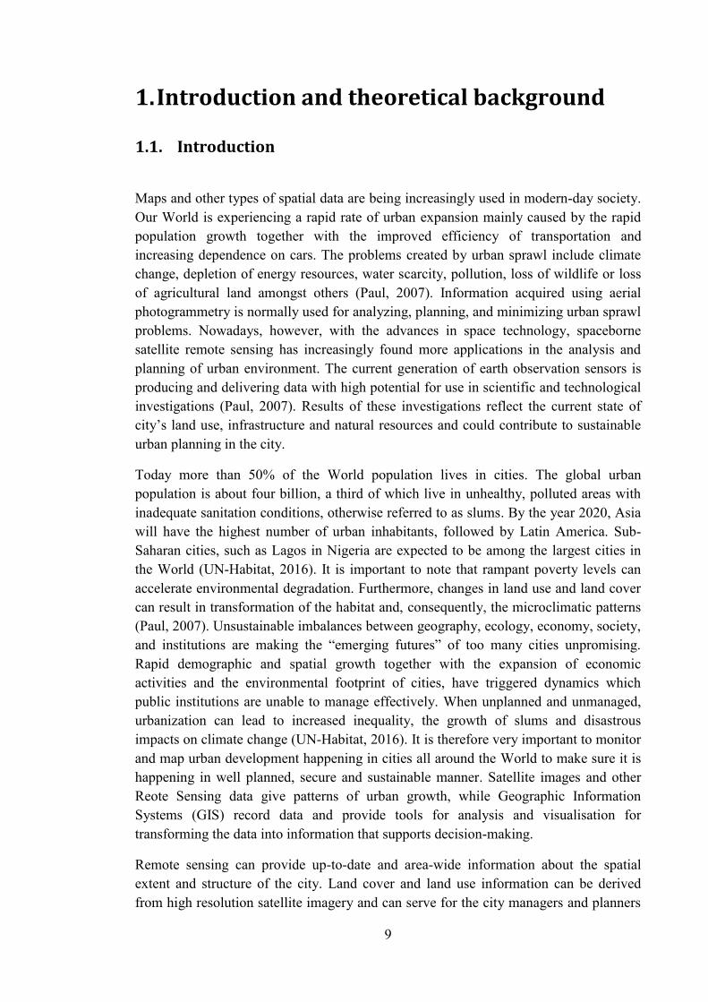
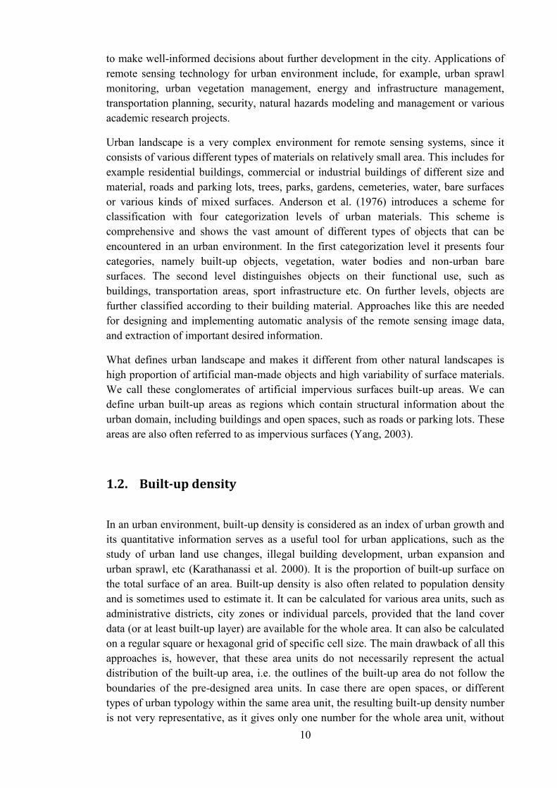


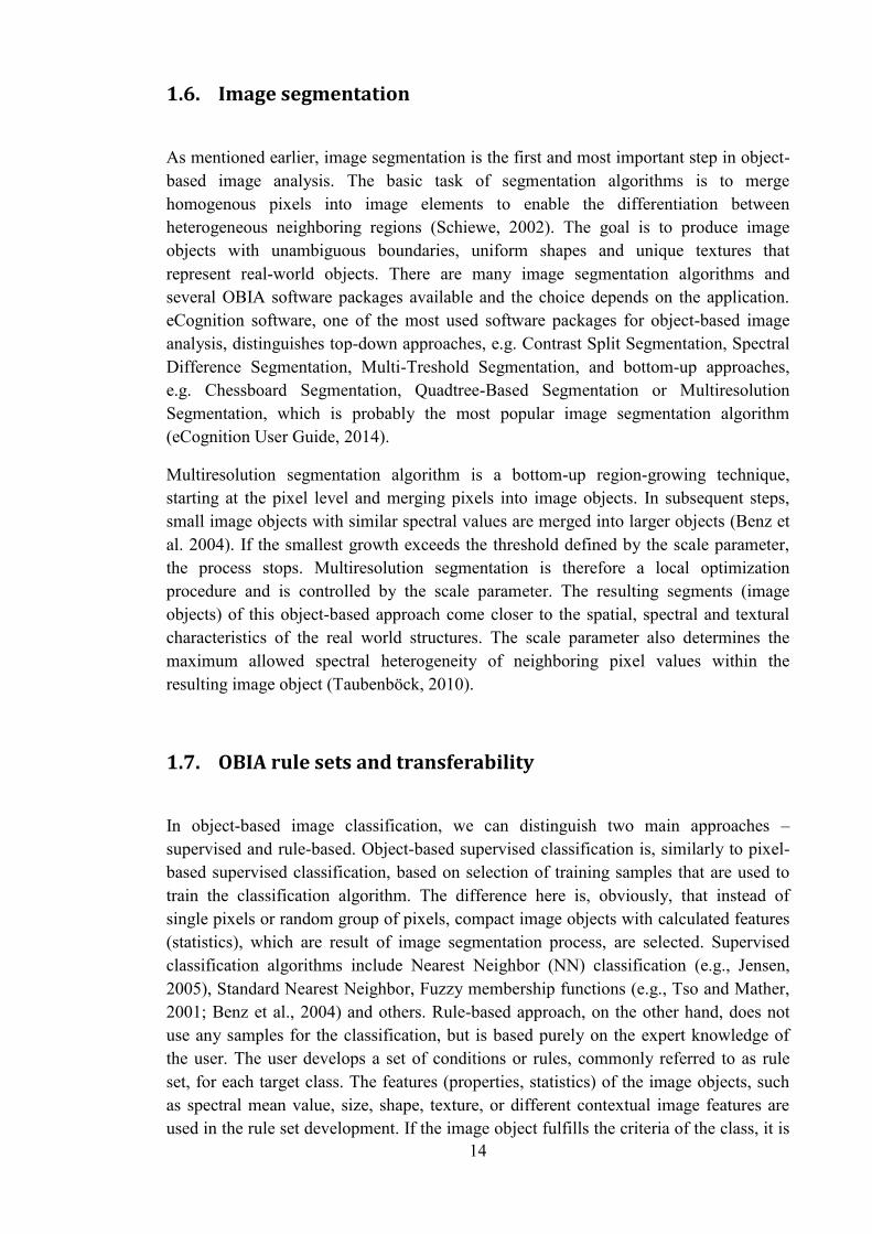


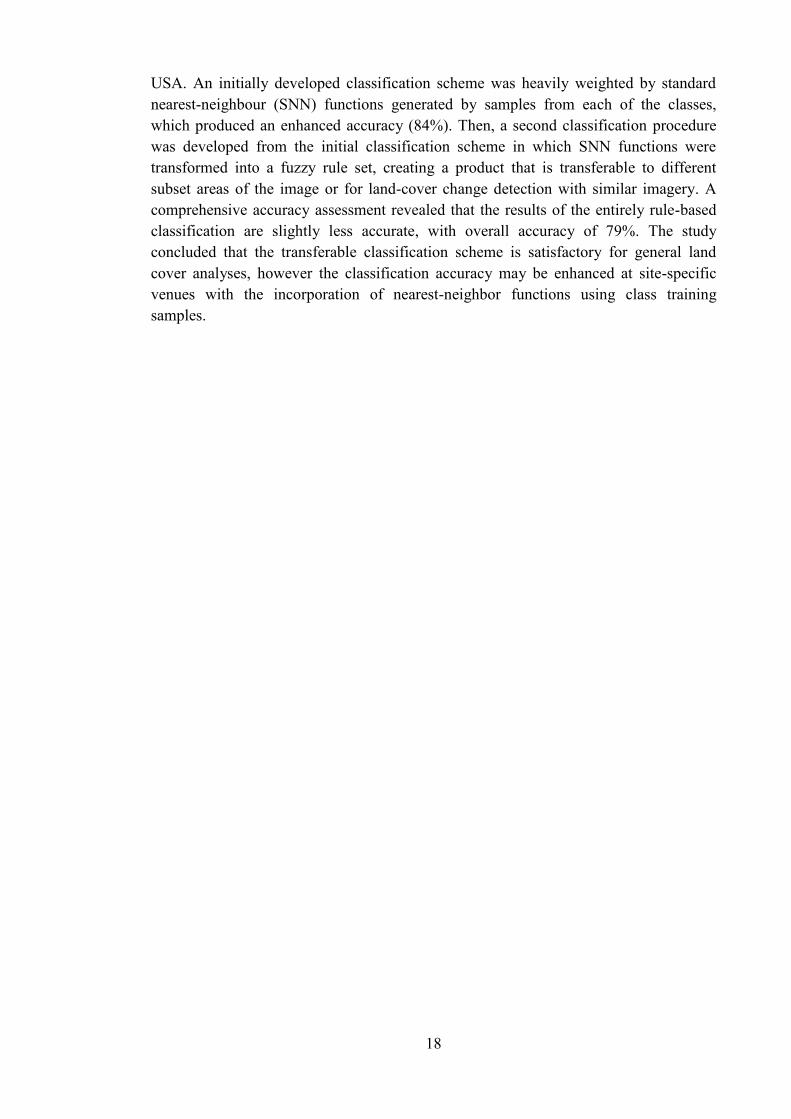
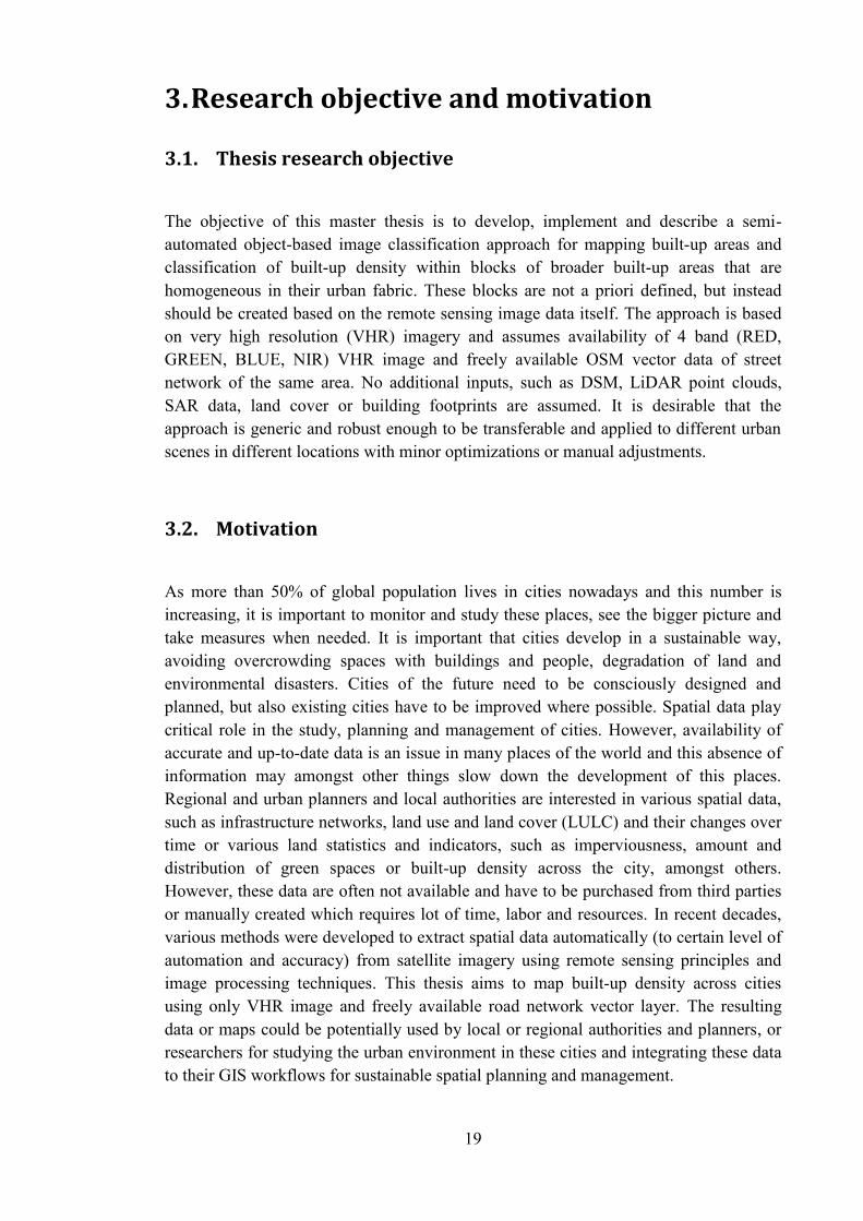
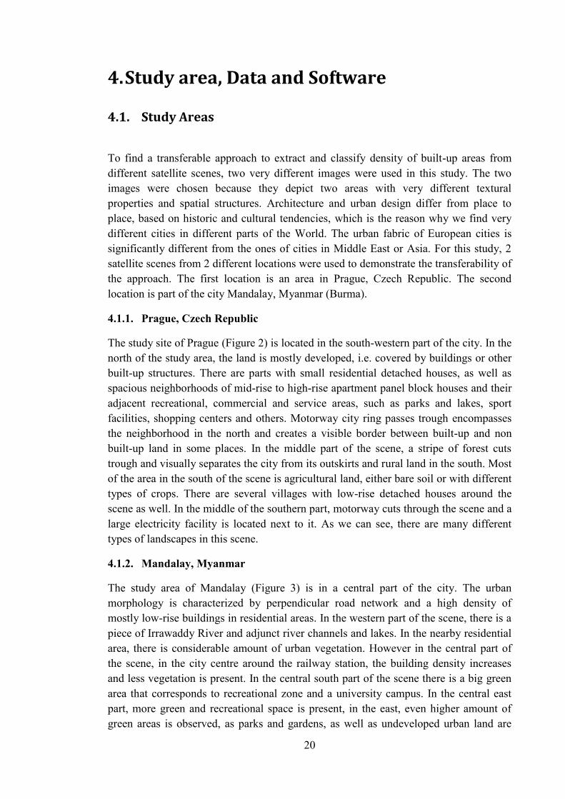
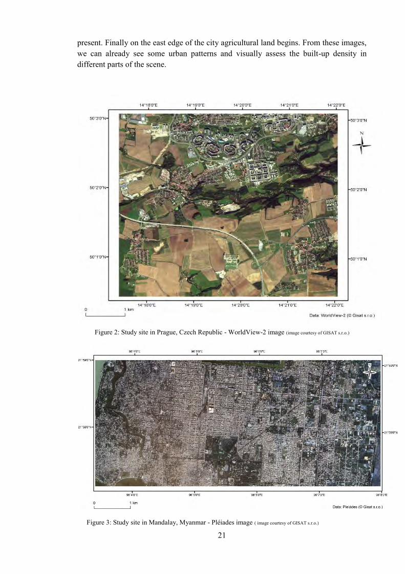
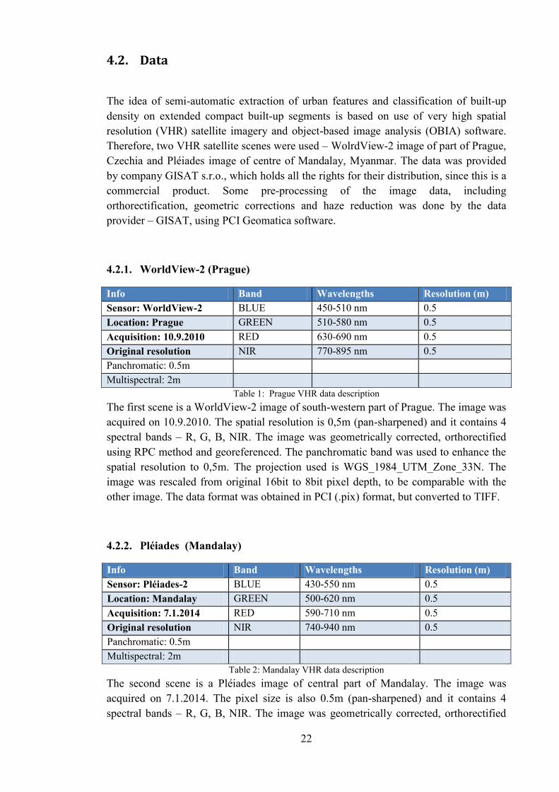
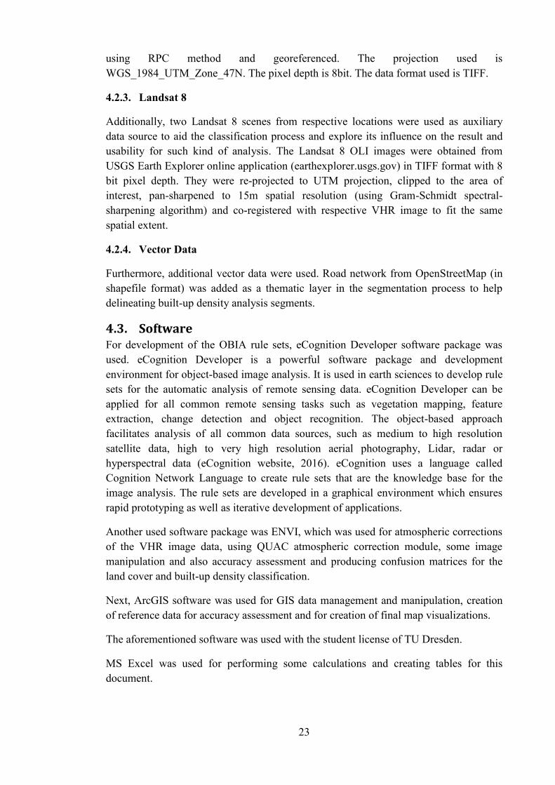
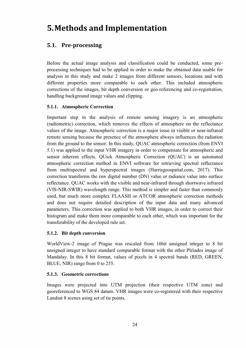
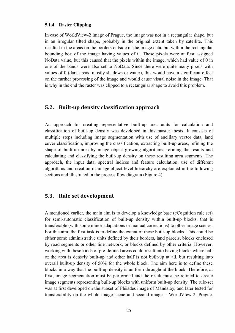

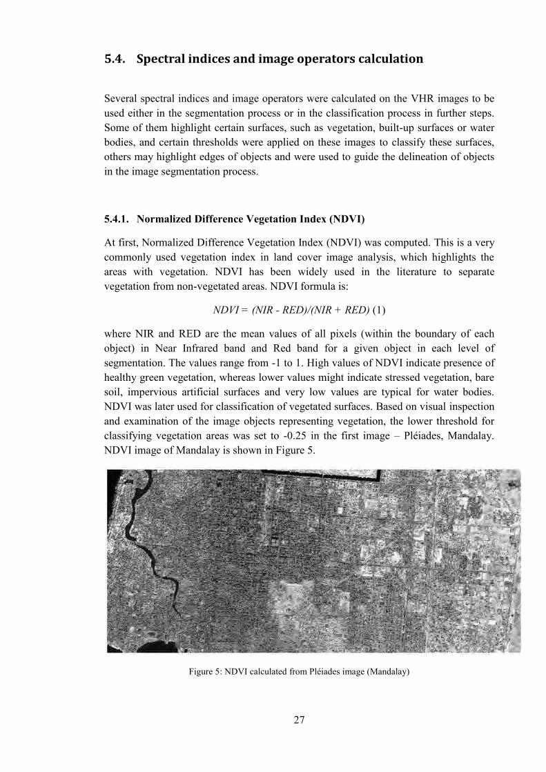
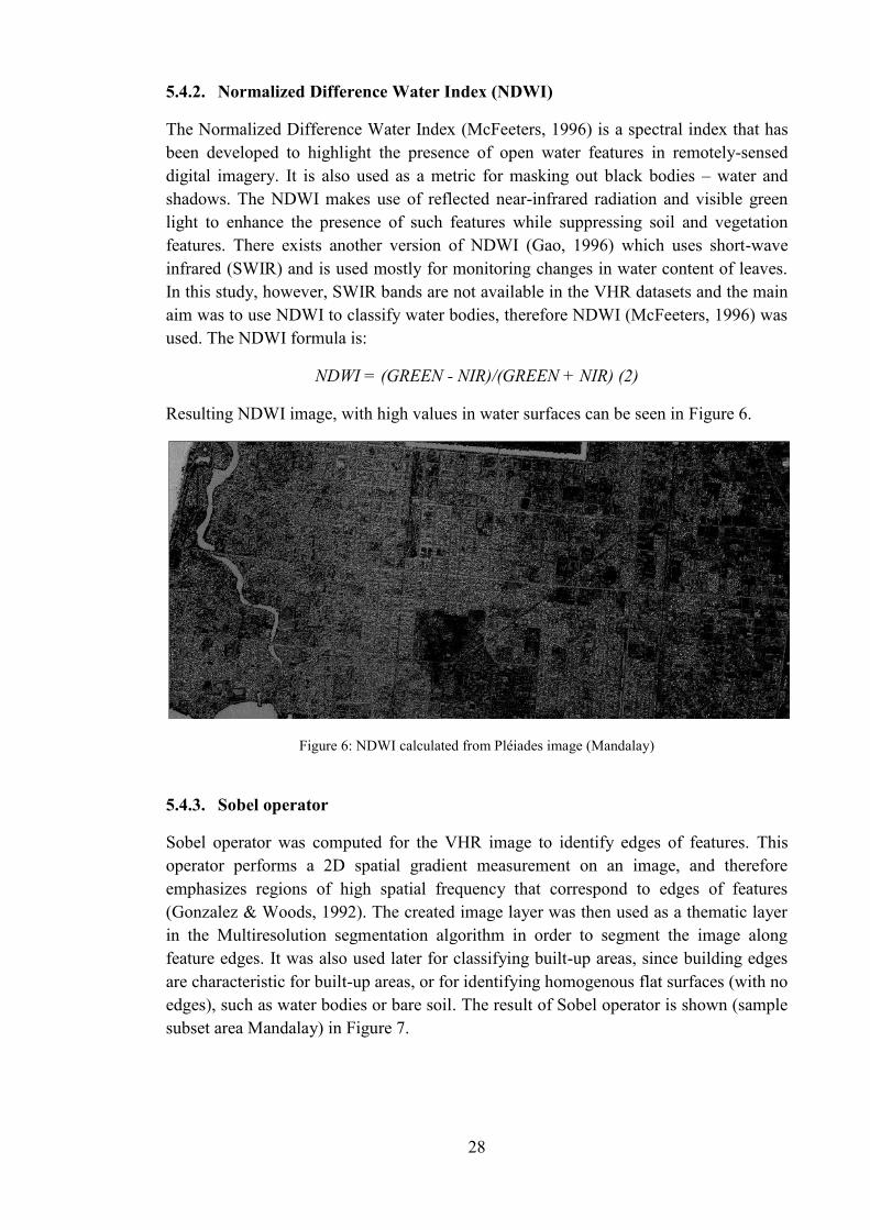
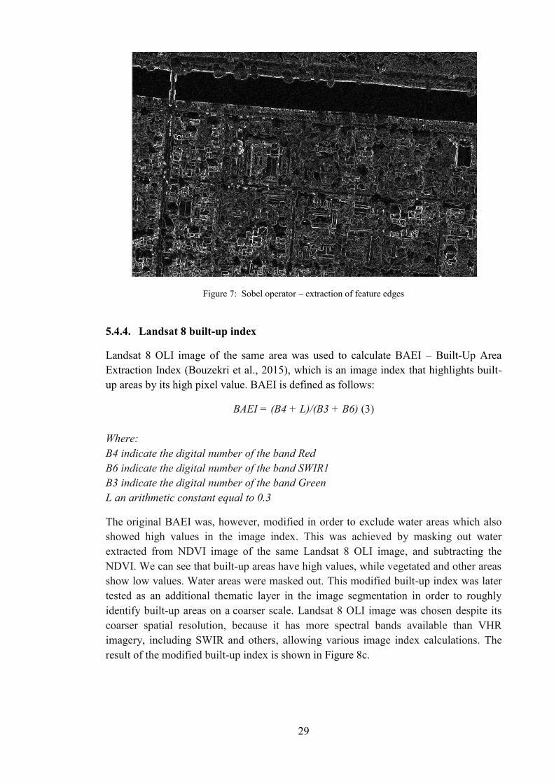
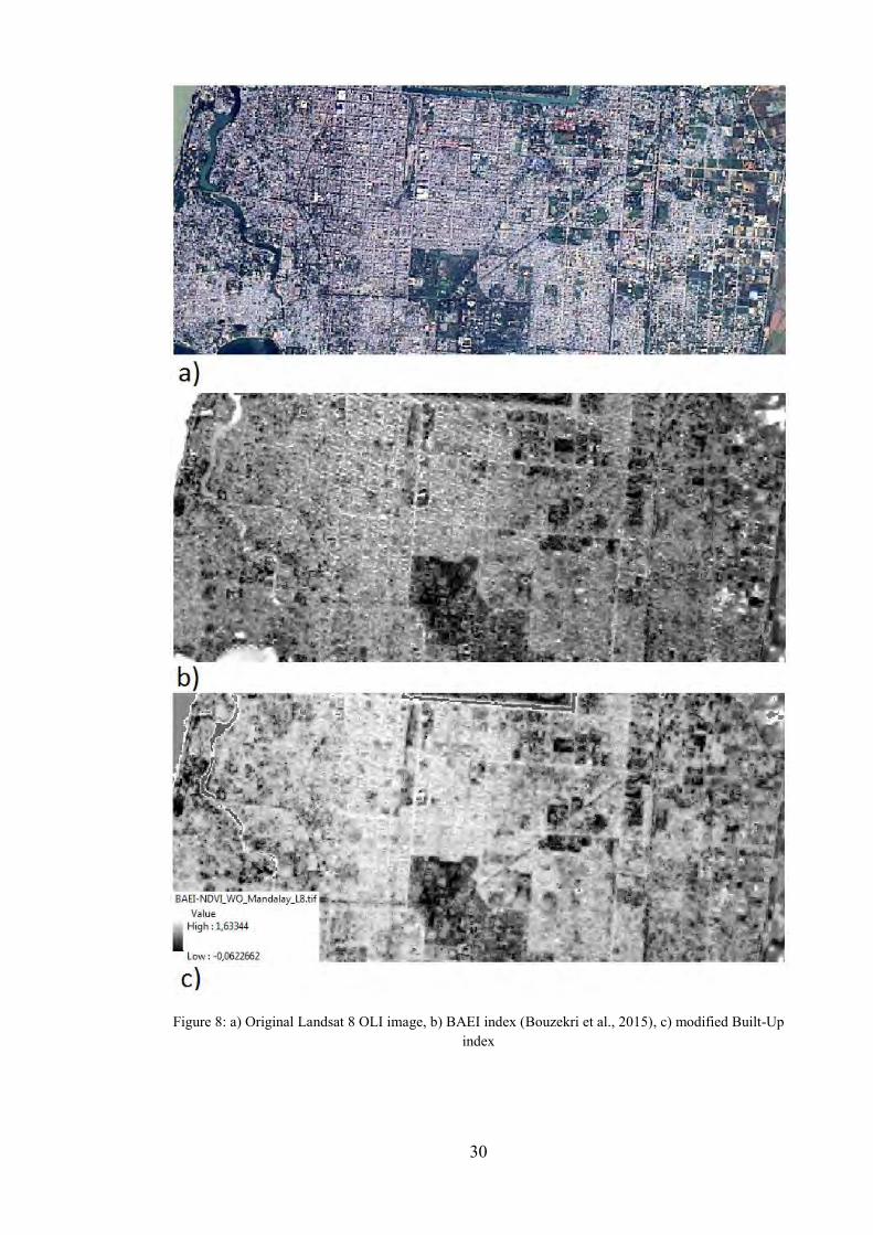


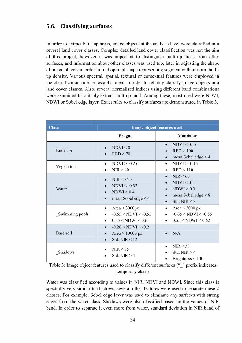

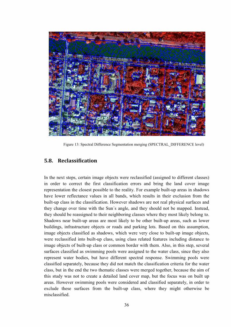

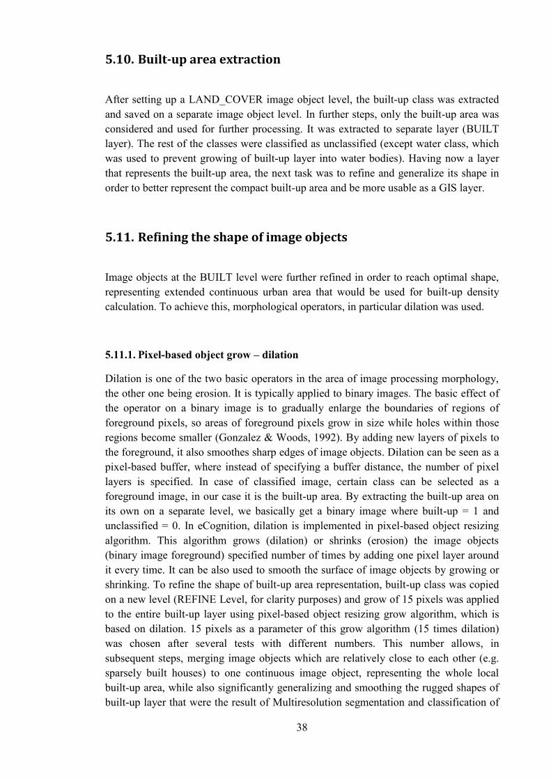
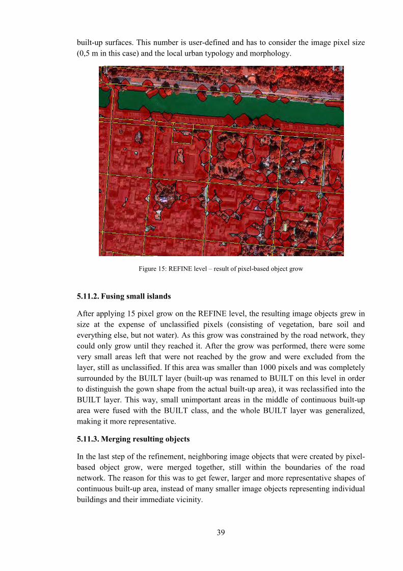
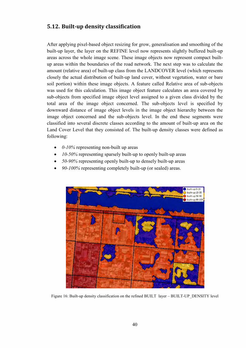
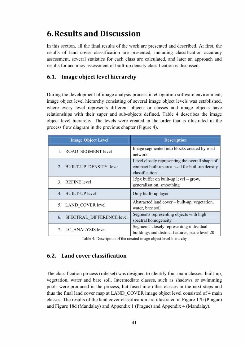
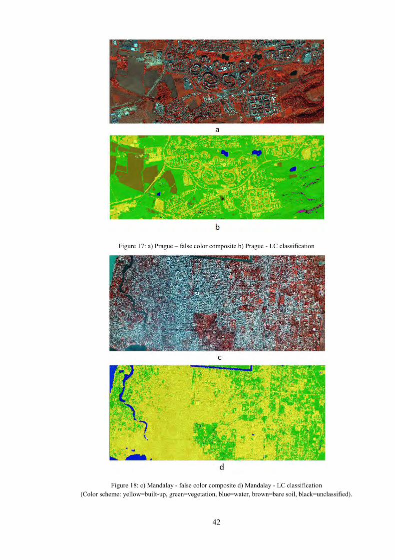
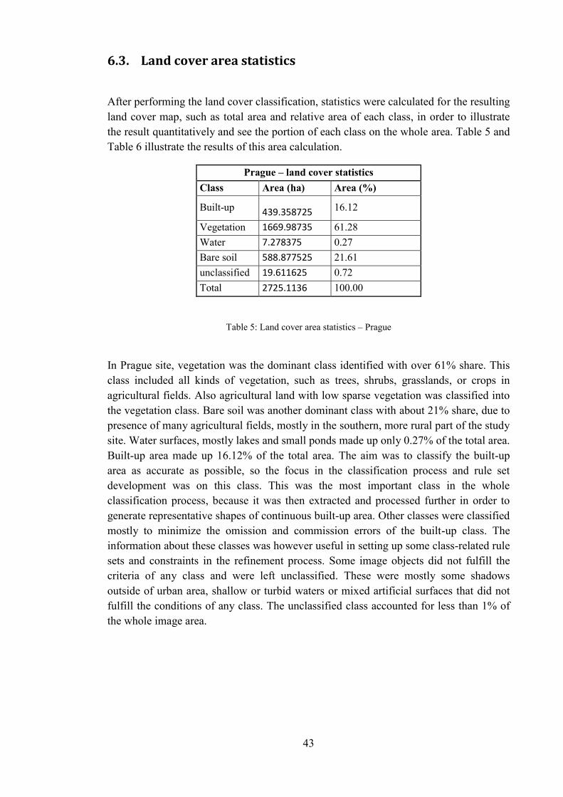
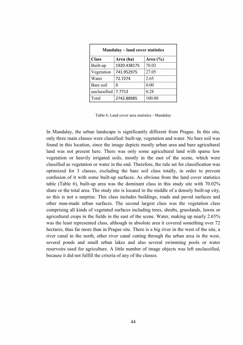
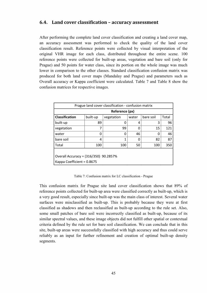
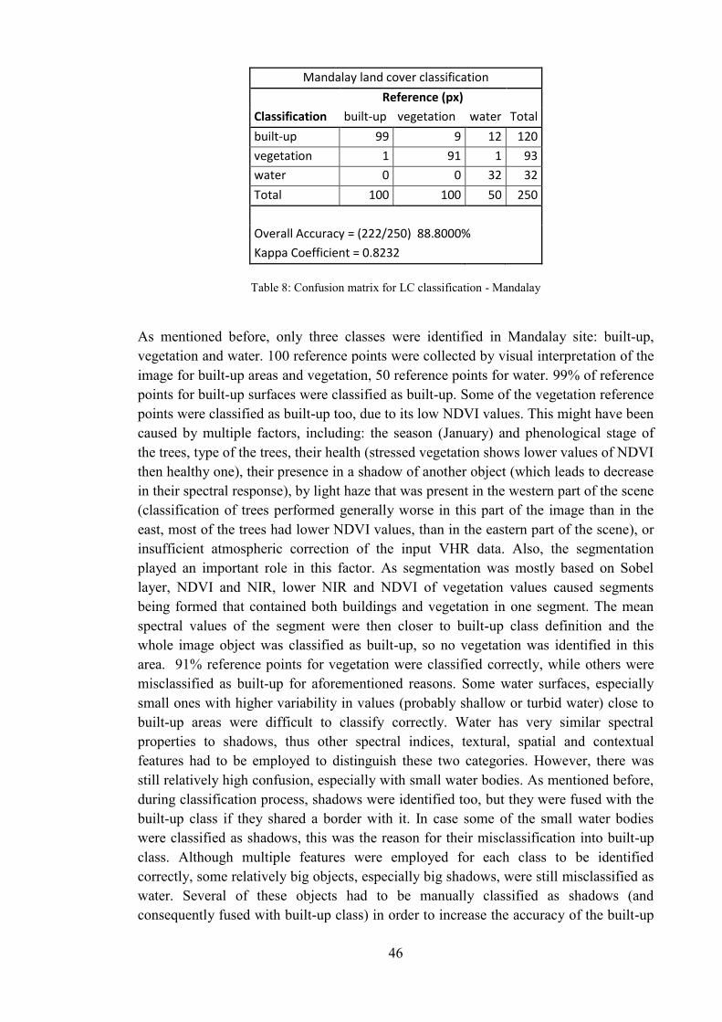
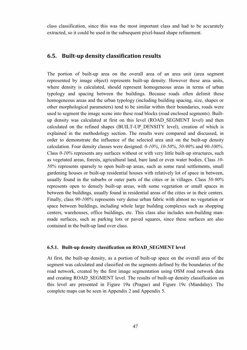
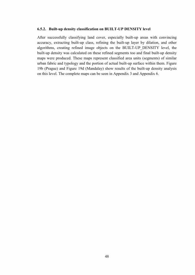


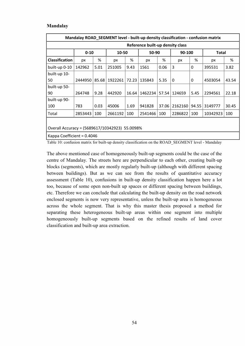
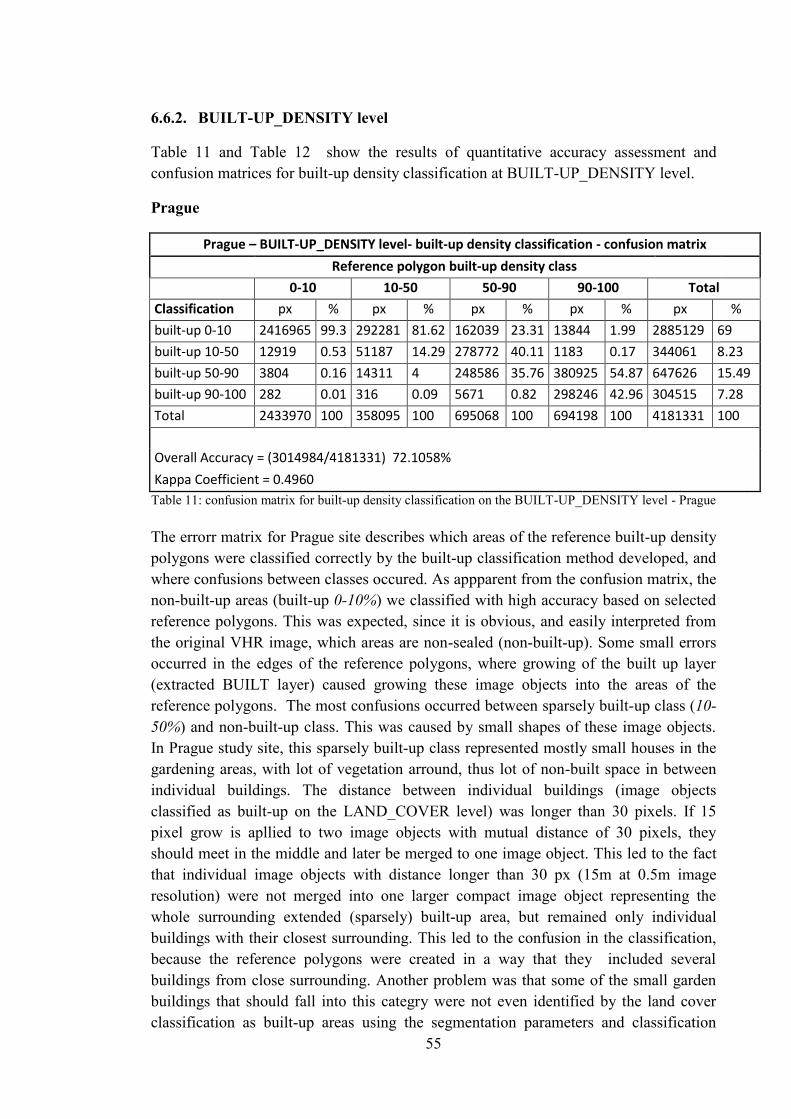
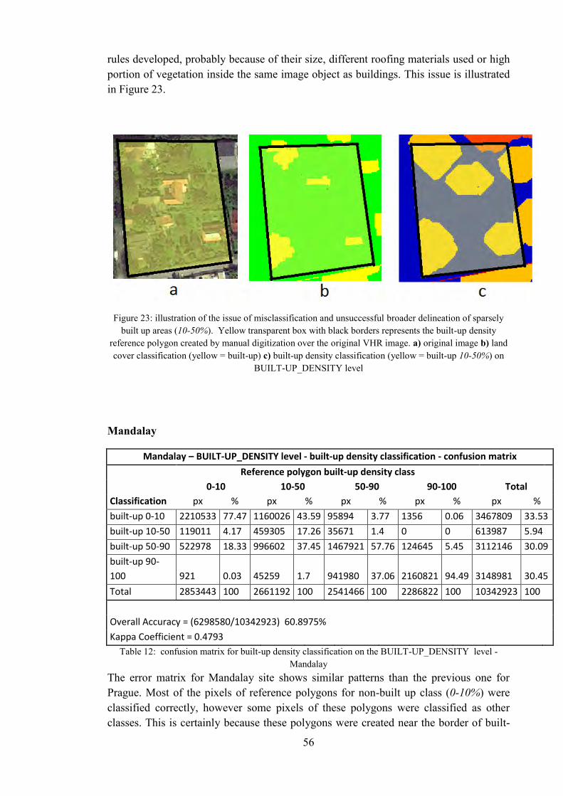

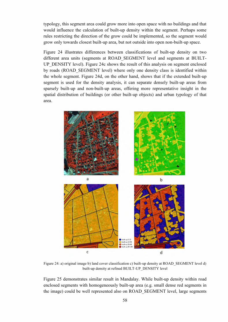
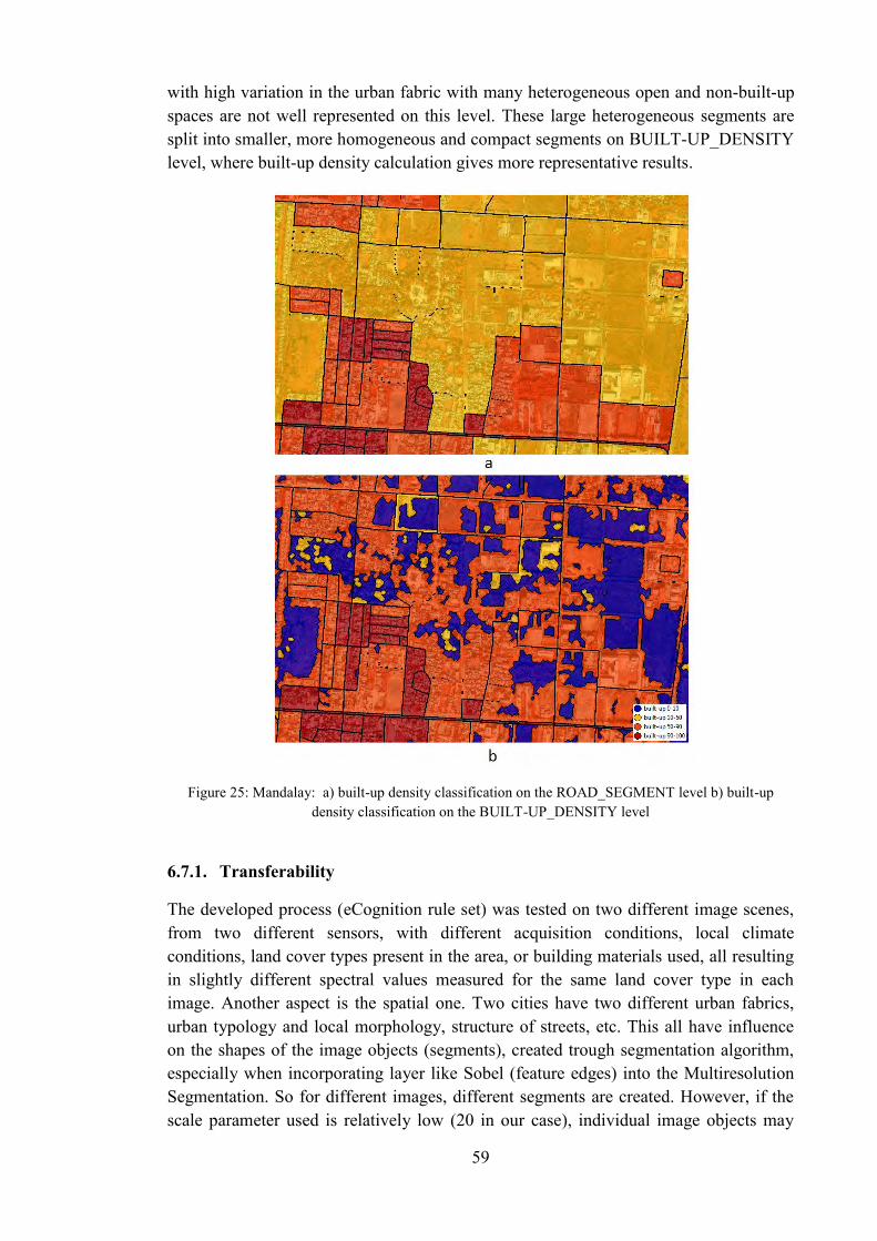


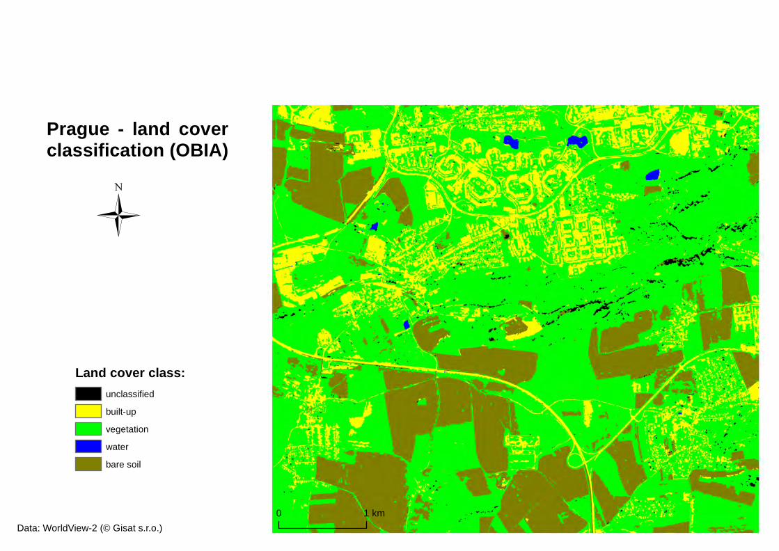
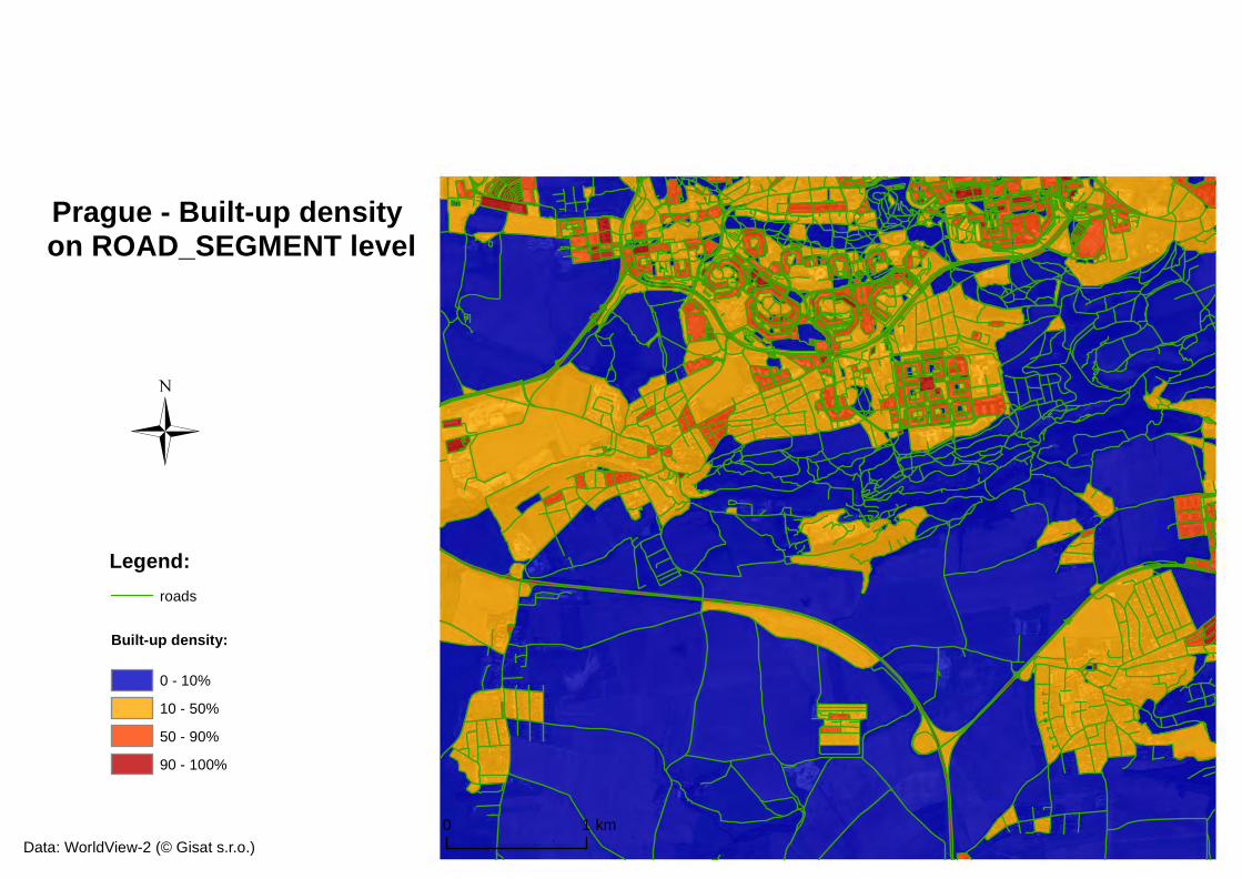
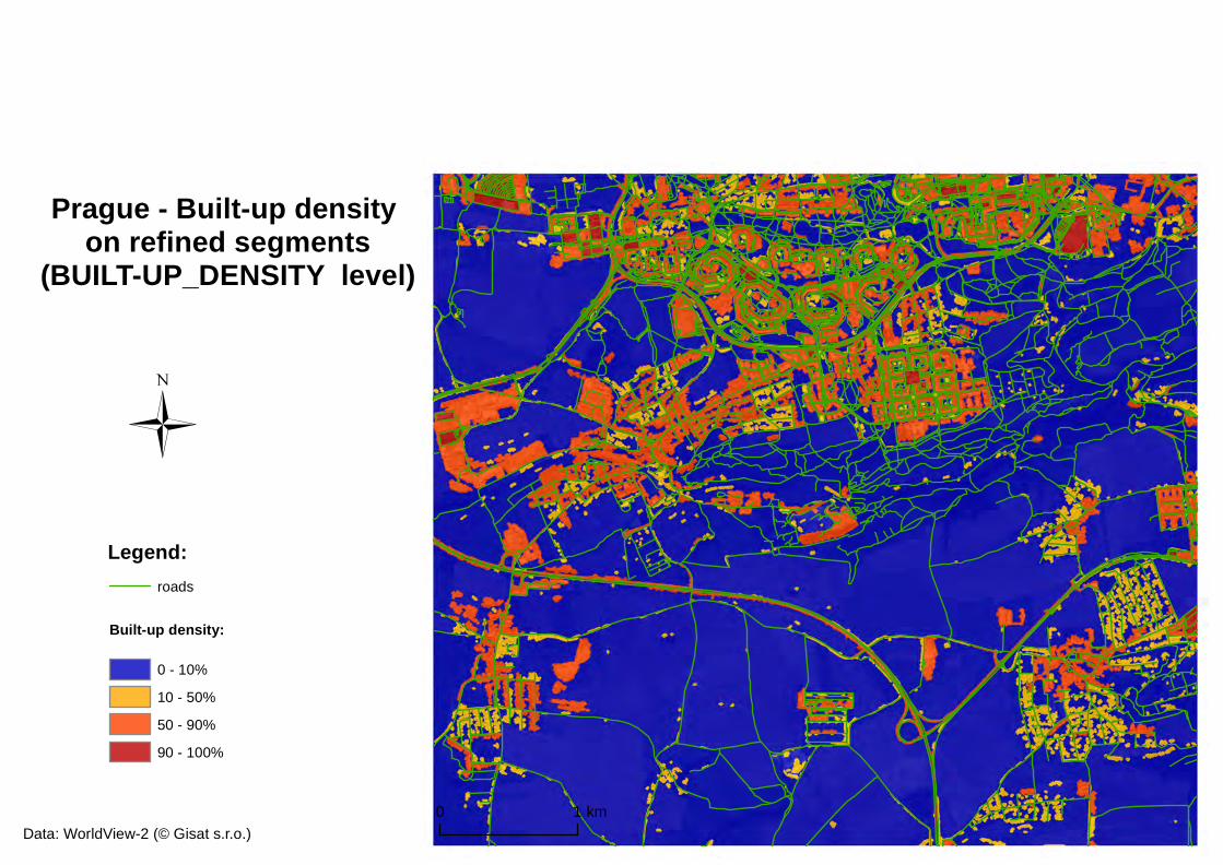

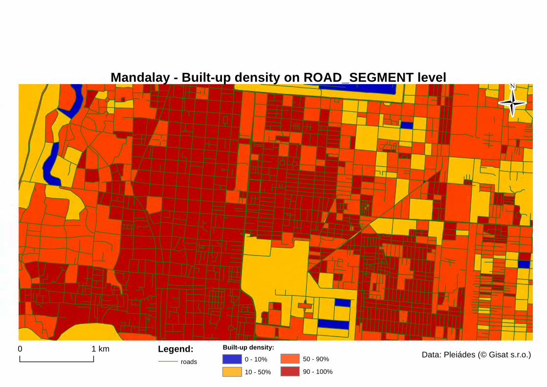
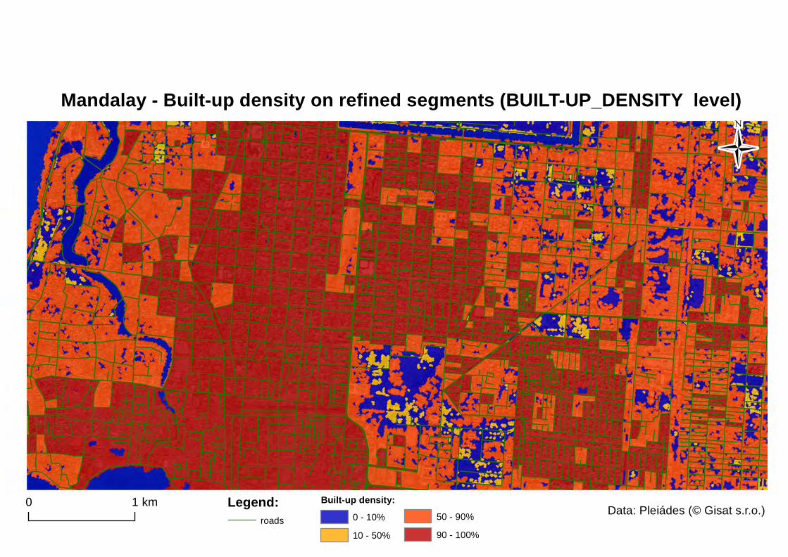

![Bachelor-, Master- and PhD Theses in Experimental …nisius/Theses.pdf · Bachelor-, Master- and PhD Theses in Experimental Particle Physics within the ATLAS SCT Group [GeV] at the](https://static.documents.pub/doc/80x56/5baa06f909d3f28b6f8d5b20/bachelor-master-and-phd-theses-in-experimental-nisius-bachelor-master-.jpg)


