Master Thesis - flex.phys.tohoku.ac.jp

Master Thesis

Surface plasmon in hollow metallic cylinder

Tian Yuan

Department of Physics, Graduate School of Science

Tohoku University

July 2020

Acknowledgments

In this acknowledgment, I would like to thank everyone who has supported me in

�nishing my master course and this thesis. First, I would like to express my gratitude

to Saito-sensei for his help and guidance not only on �nishing my master course. He

taught me not only how to conduct physics researches, but also how to present my ideas

and communicate with other researchers, which is very important for doing researches

in modern days. I also want to express my thankfulness to my families, especially my

father, who supported me since I was very young. I would also like to express my

special gratitude towards Sho�e-san, who have helped me so much as good listener

and teacher, and help me a lot at my research. For all of my lab mates : Nuguhara-

san, Nguyen-san, Pratama-san, Shirakura-san, Iwasaki-san, Islam-san, Maruoka-san,

Wang-san, Pang-san, Maeda-san, It has been a great time to work with you all.

The last but not the least, I would like to address my thankfulness to Tohoku

University and IGPAS program for giving me the chance to study and to do research

in Japan. This has been my unforgettable experience and I am so lucky to have it.

I also acknowledge the support of GP-Spin program at Tohoku University, without

which support this research cannot be �nished.

iii

Contents

Acknowledgments iii

Contents v

1 Introduction 1

1.1 Purpose of the study . . . . . . . . . . . . . . . . . . . . . . . . . . . . 1

1.2 Background . . . . . . . . . . . . . . . . . . . . . . . . . . . . . . . . . 2

1.2.1 Plasmon and surface plasmon oscillation . . . . . . . . . . . . . 2

1.2.2 The Drude model . . . . . . . . . . . . . . . . . . . . . . . . . . 4

1.2.3 Surface plasmon and near �eld enhancement . . . . . . . . . . 6

2 Electromagnetic wave on cylindrical system 13

2.1 The Helmholtz equation in cylindrical system . . . . . . . . . . . . . . 13

2.1.1 Surface plasmons propagating in azimuthal direction . . . . . . 17

2.1.2 Surface plasmons propagating along axial direction . . . . . . . 21

2.1.3 Elliptical surface plasmon . . . . . . . . . . . . . . . . . . . . . 23

2.2 Surface modes on hollow cylinder . . . . . . . . . . . . . . . . . . . . . 27

2.3 Enhancement and the incident light . . . . . . . . . . . . . . . . . . . 32

3 Enhancement of electric �eld around the hollow cylinder 35

3.1 The spatial distribution of electric �eld in the hollow cylinder . . . . 35

4 The analytical expression of enhancement of electric �eld in a

metallic hollow cylinder 39

4.1 The �tting of enhancement spectra . . . . . . . . . . . . . . . . . . . . 39

4.2 Critical geometry and optimized geometry . . . . . . . . . . . . . . . . 45

v

5 Conclusions 47

A Calculation Programs 49

A.1 Dispersion for axial surface plasmon in hollow cylinder . . . . . . . . . 49

A.2 Dispersion and the enhancement for azimuthal surface plasmon in hol-

low cylinder . . . . . . . . . . . . . . . . . . . . . . . . . . . . . . . . . 50

A.3 Enhancement spectrum and the �tting . . . . . . . . . . . . . . . . . . 50

Bibliography 53

vi

Chapter 1

Introduction

1.1 Purpose of the study

Enhancement of electromagnetic (EM) �eld around a metallic nanocylinder is a phe-

nomenon used in a lot of applications, since a metallic nano cylinder with or without

a hollow core represents a tip used in tip-enhanced Raman spectroscopy (TERS) [1,

2, 3, 4] and a probe used in scanning near�eld optical microscopy (SNOM) [5, 6].

On the surface of the tip, a strong enhancement of the EM �eld occurs by surface

plasmon (SP), which enhances the signal of TERS and SNOM. Furthermore, since

the enhancement occurs at the scale of nanometer, the spatial resolution improves

much compared with the wavelength of light. The enhancement around the metallic

nanotube also has a potential application for increasing the e�ciency of photovoltaic

cell [7]. Thus designing a nano-structure with a strong enhancement of the EM �eld

can also help to increase optical absorption or to generate a heat on sample, which is

the purpose of this thesis.

The experimental and theoretical researches have shown that the strong enhance-

ment in a metallic cylinder could come from an elementary excitation referred as a SP,

which is a collective oscillation of charge density on the surface. The existence and

properties of SP on metallic nanocylinder have been studied extensively [8, 1, 9], and

it is already been observed in the experiments that SP in nanocylinder is excited by

infra-red light. However, even though the existence of SP in a metallic nanocylinder

is already studied and well proved, designing the cylinder which gives a strong en-

1

2 Chapter 1. Introduction

hancement is not easy as a function of the frequency or the diameter of the core, since

that we have no analytical expression of the enhancement. If the relationship between

the enhancement of the electric �eld and the frequency for a given geometry of the

light is available, we could synthesize cylinders that gives the best enhancement for a

given frequency of the light. In this thesis, we focus on a hollow nano cylinder with a

hollow core. The purpose of this work is to analyze the properties of SPs on the nano

cylindrical structures, especially the enhancement of electric �eld in the hollow core

caused by SPs, and to represent such enhancement as a function of the geometrical

parameters of the cylinder and the frequency of the incident light. In the present

thesis, we solve the Helmholtz equation for a EM wave around the cylinder by using

several boundary conditions. By solving the equations, we could get the enhancement

numerically as a function of the geometrical parameters and incident light frequency,

from which we can �t the enhancement to a single function. Such �tted result would

be compared with the dispersion of SP.

This master thesis is organized as follows. In the remaining part of Chapter 1 we

introduces the background for the present research to help understanding the thesis.

In Chapter 2, we discuss the method to calculate the enhancement of EM �eld in

cylindrical system and the calculated energy dispersion of di�erent types of SPs. In

Chapter 3, we analyse the enhancement of EM wave by changing the geometrical

parameters of the system. In Chapter 4, we will discuss the �tted analytical expressions

of the enhancement, absorption probability and other properties of the enhancement.

In Chapter 5, we give conclusion of the thesis.

1.2 Background

Here we show some basic concepts which are important for understanding this thesis.

1.2.1 Plasmon and surface plasmon oscillation

Plasma refers to a state of material, in which the positive and negative charges in the

material are unbounded or weakly bounded by the Coloumb interaction to each other

and delocalized. In the metals, since the electrons can move in a background of positive

ions, an electron plasma can be excited. A plasmon is an elementary excitation of the

1.2. Background 3

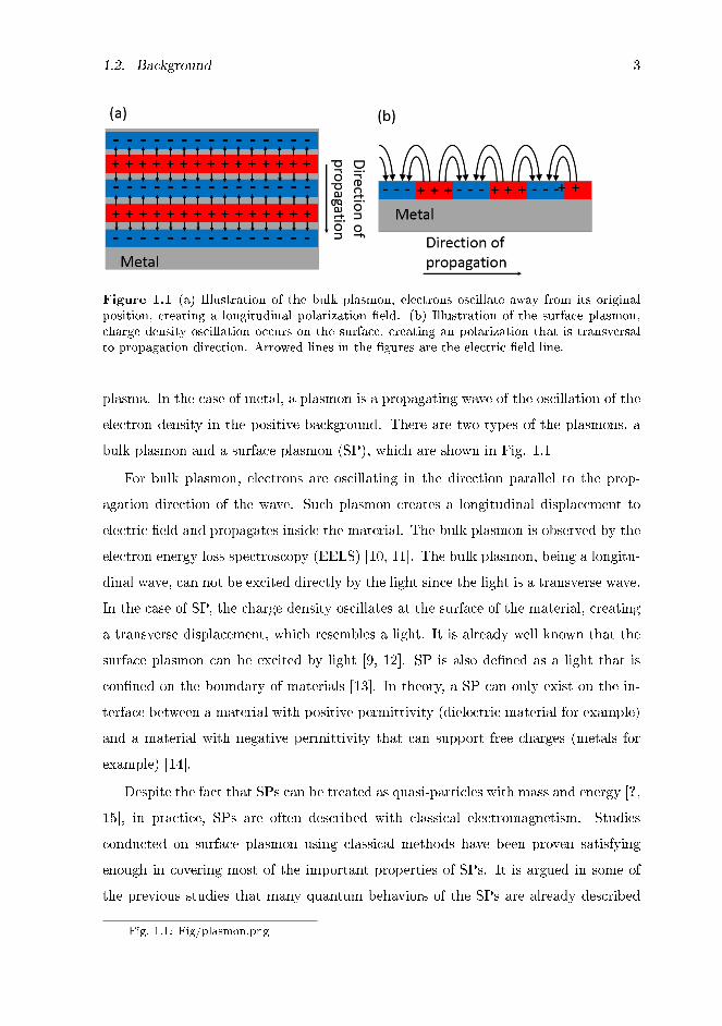
Figure 1.1 (a) Illustration of the bulk plasmon, electrons oscillate away from its originalposition, creating a longitudinal polarization �eld. (b) Illustration of the surface plasmon,charge density oscillation occurs on the surface, creating an polarization that is transversalto propagation direction. Arrowed lines in the �gures are the electric �eld line.

plasma. In the case of metal, a plasmon is a propagating wave of the oscillation of the

electron density in the positive background. There are two types of the plasmons, a

bulk plasmon and a surface plasmon (SP), which are shown in Fig. 1.1

For bulk plasmon, electrons are oscillating in the direction parallel to the prop-

agation direction of the wave. Such plasmon creates a longitudinal displacement to

electric �eld and propagates inside the material. The bulk plasmon is observed by the

electron energy loss spectroscopy (EELS) [10, 11]. The bulk plasmon, being a longitu-

dinal wave, can not be excited directly by the light since the light is a transverse wave.

In the case of SP, the charge density oscillates at the surface of the material, creating

a transverse displacement, which resembles a light. It is already well known that the

surface plasmon can be excited by light [9, 12]. SP is also de�ned as a light that is

con�ned on the boundary of materials [13]. In theory, a SP can only exist on the in-

terface between a material with positive permittivity (dielectric material for example)

and a material with negative permittivity that can support free charges (metals for

example) [14].

Despite the fact that SPs can be treated as quasi-particles with mass and energy [?,

15], in practice, SPs are often described with classical electromagnetism. Studies

conducted on surface plasmon using classical methods have been proven satisfying

enough in covering most of the important properties of SPs. It is argued in some of

the previous studies that many quantum behaviors of the SPs are already described

Fig. 1.1: Fig/plasmon.png


Figure 1.2 (a) The schematic of the Drude model, electrons moves freely in a backgroundof positive ions. (b) The electrons are displaced with a distance x with respect to the back-ground, in a volume with the cross section A.

within the dielectric function describing metal permittivity [10, 12, 16].

1.2.2 The Drude model

Since SP is a quantum of collective motion of electrons, it is important for us to

describe an electron in a metal. The Drude model or free electron model is a classical

model for describing the behavior of electron. In this model, the electron is treated as

a free particle that moves in a background of positive ionic cores, as is shown in Fig.

1.2 (a). Equation of motion of the electron in the electric �eld is given by,

md2[r(t)]

dt2+m

τ

d[r(t)]

dt= −eE(t), (1.1)

where m denotes the mass of the electron, r(t) is the position of the electron, τ is a

relaxation time, which means an average time of a electron to lose the kinetic energy,

e stands for the elementary charge and E(t) is a time-dependent external electric

�eld [12]. Let us consider the harmonic time-dependence for E(t) and r(t) given as

follows:

E(t) = E0e−iωt, (1.2)

r(t) = r0e−iωt. (1.3)

Fig. 1.2: Fig/drudedielec.png

1.2. Background 5

By substituting Eqs. (1.2) and (1.3) into Eq. (1.1), we can get the following equations.

−mω2r(t)− im

τωr(t) = −eE(t),

r(t) =eE(t)

mω2 + im/τ. (1.4)

By setting γ = 1/τ as the damping rate, an induced electric polarization is given by

r(t) as follows:

Pe(t) = −ner(t) = − ne2

mω2 + iγωE(t), (1.5)

where n refers to the number density of electrons. By adding Eqs. (1.5) with the

polarization of the background Pb, we obtain the total polarization of a metal as

follows [17]:

P(t) = Pb(t) + Pe(t) =

(χb −

ne2

mω2 + imγω

)E(t), (1.6)

where χb is the background polarizability. The electric displacement vector in the

metal is given by

D(t) = εrε0E(t) = ε0E(t) + P(t)

= ε0

[1 + χb/ε0 −

ne2

mε0(ω2 + iγω)

]E(t). (1.7)

By de�ning the relative permittivity of the background as: εb = 1 +χb/ε0, we get the

relative permittivity of metal εr from the Drude model as follows:

εr(ω) = εb −ω2p

ω2 + iγω, (1.8)

where we de�ne the bulk plasmon frequency ωp as follows:

ωp =

√ne2

mε0. (1.9)

To understand the physical meaning of ωp, we will now derive the bulk plasmon

frequency ωp of a metal by considering the situation where free electrons in a volume

of space with cross sectional area A has been displaced with distance r, as is shown

in Fig. 1.2 (b). From the Gauss law, we can get the electric �eld caused by such

displacement as follows:

E =Q

Aε0=neAr

Aε0

=ner

ε0. (1.10)


By substituting Eq. (1.10) into Eq. (1.1) and assuming that there is no collision of

electrons i.e. 1/τ = γ = 0, we get

nmd2r

dt2= −neE

= −n2e2r

ε0⇐⇒ d2r

dt2+ne2

mε0r = 0. (1.11)

Eq. (1.11) describes the motion of free electron gas under a self-sustaining electric �eld,

which is an equation of motion of an harmonic oscillator. This equation describes

an intrinsic oscillation of electrons in metal, whose frequency is the bulk plasmon

frequency ωp =√

ne2

mε0[12].

We �nd that the permittivity in Eqs. (1.9) is a function of incident light frquency

ω. It is noted that ωp is only related to the electron density n. On the other hand γ

is related to the Fermi velocity vF and electron mean free path l as: γ = 1/τ = vF /l.

For an ideal metal, the permittivity is calculated as a function of n, l, vF and εb.

However, actual metals under common circumstances and optical frequencies are not

ideal conductors. E�ective parameters �tted from data gatherd in experiment is used

in actual study [18, 19, 1]. With the electric permittivity derived, we are ready to start

the mathematical description of SPs starting from the classical electromagnetism. The

description of SPs using the classical electromagnetism is appropriate when the size of

the material is larger than 10 nm. Otherwise the quantum description should be used.

For the calculations in this thesis, we are going to focus on the phenomena happening

on gold structures. The parameters were taken: εb = 5.9673, ωd/(2π) = 2113.6 THz,

γ = 15.92 THz [20].

1.2.3 Surface plasmon and near �eld enhancement

Next we want to introduce some applications, excitation and observation of SPs in

experiments, then we will present a simple numerical descriptions of a certain type of

SPs.

The SP is a well observed phenomenon that has been used for a wide range of

applications. The earliest phenomenon observed which is later proven to be related to

the SPs, is color-stained glass due to the absorption of the light caused by localized SP

resonance on noble metal particles [12]. Such technique of color-staining was �st used

in fourth century Europe but without a good physical explanation until the theory of

1.2. Background 7

plasmonics was developed. It is understood now that such coloring is caused by the

optical absorption due to the excitation of SPs. Beside staining the glass, local �eld

enhancement and optical absorption by localized SP resonance on metallic particles

also �nd more modern applications in photovoltaic devices [12, 9], bio science/medical

detection [21] and spectroscopies [22]. Such localized SPs can also be found on a

cylinder when SPs oscillate around the circumference of the cylinder [23, 24].

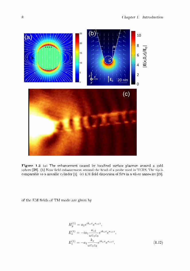
As has been proven in experiments, localized SPs can be excited by directly shading

light on a metallic sphere or a cylinder. The excitation induces a strong near �eld

enhancement, as is shown in Fig. 1.3 (a) and (b). This is one of the easiest ways to

excite SPs, with many detailed researches and experiments conducted to observe and

utilize the near �eld enhancement. It is noted that besides a localized SP, a cylinder can

also support a SP that propagates in axial direction, as is shown in Fig. 1.3 (c). In most

of actual experiments, both the localized and the propagating SPs are excited [25, 26].

The near �eld enhancement around the cylinder could �nd similar uses as that around

sphere, such as enhancing the EM �eld intensity, increasing the absorption of the light

and increasing signal intensity in spectroscopies. SPs propagating along axial direction

of a cylinder can be excited by an incident light in one tip of the cylinder and emit

the light on the other tip, which is capable of carrying the information along the axis

of the cylinder [27].

The most mathematically intuitive case of a SP is a propagating SP on a �at sur-

face. In the following discussion we want to provide a simple analysis of SP on a �at

surface to serve as a simple example for understanding more mathematically compli-

cated cases of SPs on a cylinder. By solving the Maxwell equations on a �at surface,

we will get two groups of equation, each group de�nes a solution of a speci�c surface

wave mode. More speci�cally, by assuming that the surface wave mode propagates in

the x-direction with wave vector kx, we can get the EM �elds of the surface modes as

is shown in Fig. 1.4.

Let us start with one of solution of the surface mode, which is shown in Fig. 1.4

(a). The mode has in-plane magnetic �eld that is transverse to propagation direction,

hence such mode was refereed as a transverse magnetic (TM) mode. The expressions

Fig. 1.3: Fig/samples.pngFig. 1.4: Fig/�at-sp.PNG


Figure 1.3 (a) The enhancement caused by localized surface plasmon around a goldsphere [28]. (b) Near �eld enhancement around the head of a probe used in TERS. The tip iscomparable to a metallic cylinder [1]. (c) EM �eld dispersion of SPs in a silver nanowire [29].

of the EM �elds of TM mode are given by

H(1)y = a1e

ikxxeκz1z,

E(1)x = −ia1

κz1ωε1ε0

eikxxeκz1z,

E(1)z = −a1

kxωε1ε0

eikxxeκz1z, (1.12)

1.2. Background 9

Figure 1.4 Schematic of surface modes on a metallic �at surface in a dielectric background,relative permittivity(permeability) of the metallic part and the dielectric part is ε1 (µ1) andε2(µ2), respectively. (a) A surface TM mode, containing a transverse electric �eld. (b) Asurface TE mode, containing a transverse magnetic �eld.

and

H(2)y = a2e

ikxxe−κz2z,

E(2)x = ia2

κz2ωε2ε0

eikxxe−κz2z,

E(2)z = −a2

kxωε2ε0

eikxxe−κz2z, (1.13)

where κz1 and κz2 are the decay constants on the z-direction, which are given as follow:

κz1 =√k2x − k20µ1ε1, (1.14)

κz2 =√k2x − k20µ2ε2, (1.15)

with µn (εn) is the relative permeability (permittivity) of the n-th medium, k0 = ω/c

is the wavevector of EM wave in the vacuum. E(n)i and H

(n)i in Eqs. (1.12) and

(1.13) denote electric and magnetic �eld intensities on i-th axis in the n-th medium,

respectively, and an is the amplitude of H(n)y . As is shown in Eqs. (1.12) and (1.13), a

TM mode has a component of electric �eld in the direction of propagation, as is shown

in Fig. 1.5 (a), which indicates that there is an displacement of the charge density

along the propagation direction, i.e. a propagating plasmon.

Fig. 1.5: Fig/distri�at-sp.PNG


Figure 1.5 (a) A surface TM mode, manifesting an oscillation of surface charge density inthe direction of propagation. (b) A surface TE mode, manifesting an oscillation of surfacecurrent density (J) perpendicular to that of the propagation direction.

The expressions of EM �elds of another group of surface mode are given as follows:

E(1)y = a1e

ikxxeκz1z,

H(1)x = −ia1

κz1ωµ1µ0

eikxxeκz1z,

H(1)z = −a1

kxωµ1µ0

eikxxeκz1z, (1.16)

and

E(2)y = a2e

ikxxe−κz2z,

H(2)x = ia2

κz2ωµ2µ0

eikxxe−κz2z,

H(2)z = −a2

kxωµ2µ0

eikxxe−κz2z, (1.17)

where the mode has a component of electric �eld only in the direction perpendicular

to that of the propagation. Hence the mode is known as the transverse electric (TE)

mode. Since the electric �eld is perpendicular to the propagation direction, TE mode

is not a surface plasmon. TE mode is composed by an oscillation of surface current

density (J), in which the direction of the current density is perpendicular to the

direction of the propagation, as is shown in Fig. 1.5 (b).

The dispersion relation of the surface mode determines the resonant condition of

the system, as a surface mode will be excited by light only when the incident light has

Fig. 1.6: Fig/disper�at.PNG

1.2. Background 11

Figure 1.6 Dispersion relation ωsp of surface plasmon on a �at silver/silica boundary and asilver/air boundary, straight line represents the dispersion of the light [12].

a frequency and a component of wavevector parallel to the surface that are equal to

those of the SP. The EM �elds of surface modes should satisfy the boundary conditions

of the EM �eld, that is, the tangential components of E and H are continuous on the

surface. For TE mode, from Eqs. (1.16) and (1.17), we get the following equations at

z = 0:

E(1)y = E(2)

y ↔ a1 = a2, (1.18)

H(1)x = H(2)

x ↔ a1κz1

ωµ1µ0= −a2

κz2ωµ2µ0

. (1.19)

From which we get the dispersion relation of the TE mode as follows:

κz1µ2 = −κz2µ1. (1.20)

By noticing that we are discussing a surface mode, both κz1 and κz2 should have to

be positive to ensure a decaying �eld on the z direction, which means either µ1 or

µ2 should be negative. Materials with negative permeability is not found in nature,

therefore the TE mode is not exited in the normal material. Some experiments had

successfully observed surface con�ned TE modes on a metamaterial [30, 31]. In this

thesis however we would not discuss the nature of the TE mode.


For TM mode, from Eqs. 1.12 and Eqs 1.13 and boundary conditions we can get

the following equations at z = 0:

H(1)y = H(2)

y ↔ a1 = a2,

E(1)x = E(2)

x ↔ a1κz1ωε1ε0

= −a2κz2ωε2ε0

.(1.21)

By using the de�nition of κz1 =√k2x − k20µ1ε1, κz2 =

√k2x − k20µ2ε2, from Eqs. (1.14)

and (1.15) we can get the dispersion relation for TM mode as follows:

kx = k0

√ε1ε2ε1 + ε2

. (1.22)

By assuming that the permittivity of medium 2, ε2, is a constant, and the permittivity

of medium 1, ε1, is the Drude dielectric function, we can get the dispersion relation of

the TM mode or SP on the �at surface as follows:

kx = k0

√ε2(ω2 − ω2

p)

ω2 − ω2p + ε2

. (1.23)

In Fig. 1.6, we show a plot of frequency ω of TM mode as a function of wavevector

kx on the boundary of silver and air (ωsp,air) and on the boundary of silver and

silica (ωsp,silica). The ω of TM mode is linear to wave vector for the small frequency

corresponding to mid or lower infra-red. For larger wave vector, the ω approaches

constant value of

ωsp =ωp√

1 + ε2, (1.24)

where ωp is the bulk plasmon frequency given in Eq. (1.9). It is noted that, for the

boundary with vacuum, the ω = ωsp/√

2. As is shown in Fig. 1.6, the dispersion of

TM mode is located at the right side of dispersion of light, which means that we have

an EM wave that is con�ned to the surface of the metal [12].

Chapter 2

Electromagnetic wave on cylindrical

system

In this chapter we will derive the expression of EM �eld in the cylindrical coordinate

for calculating the dispersion relation of SP and the enhancement of the electric �eld,

which is given in the Chapter 3. Simple cases of SP in a solid cylinder without a hollow

core was �rst examined to help identifying two types of SPs on metallic cylinder. Then

the solution of SPs on a metallic cylinder with a hollow core is presented.

2.1 The Helmholtz equation in cylindrical system

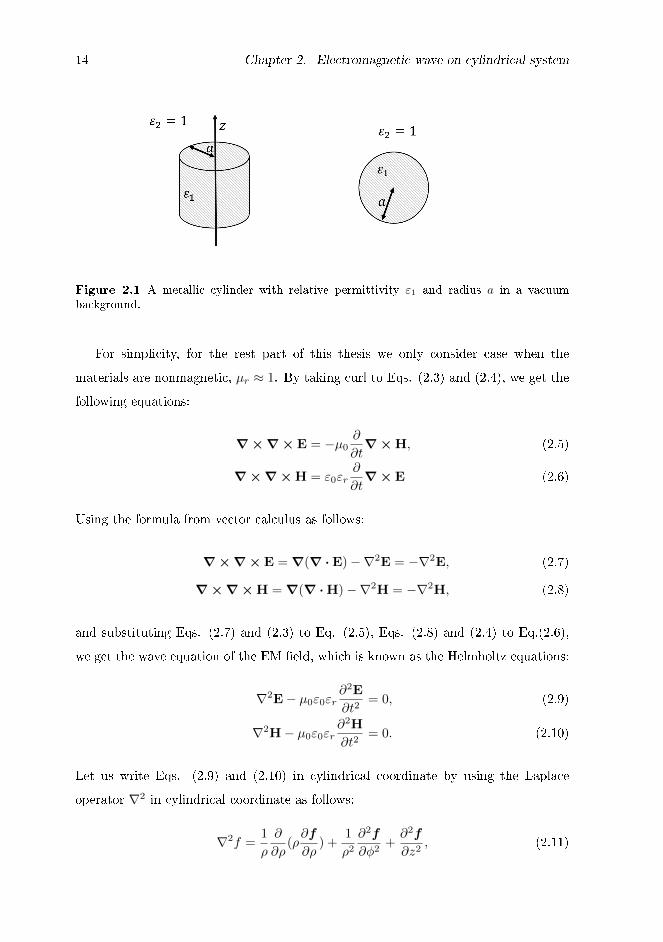
In this section we solve the SP modes on a solid metallic cylinder. In a cylindrical

coordinate, we consider a metallic cylinder with radius a that is in�nitely long in the

z-direction, with the z axis as the axis of the cylinder, as is shown in Fig. 2.1.

We start from the Maxwell equations for electric and magnetic �eld (E and H)

without any charge or current:

∇ ·E = 0, (2.1)

∇ ·H = 0, (2.2)

∇×E = −µ0µr∂H

∂t, (2.3)

∇×H = ε0εr∂E

∂(t). (2.4)

Fig. 2.1: Fig/samplesolid.PNG

13

14 Chapter 2. Electromagnetic wave on cylindrical system

Figure 2.1 A metallic cylinder with relative permittivity ε1 and radius a in a vacuumbackground.

For simplicity, for the rest part of this thesis we only consider case when the

materials are nonmagnetic, µr ≈ 1. By taking curl to Eqs. (2.3) and (2.4), we get the

following equations:

∇×∇×E = −µ0∂

∂t∇×H, (2.5)

∇×∇×H = ε0εr∂

∂t∇×E (2.6)

Using the formula from vector calculus as follows:

∇×∇×E =∇(∇ ·E)−∇2E = −∇2E, (2.7)

∇×∇×H =∇(∇ ·H)−∇2H = −∇2H, (2.8)

and substituting Eqs. (2.7) and (2.3) to Eq. (2.5), Eqs. (2.8) and (2.4) to Eq.(2.6),

we get the wave equation of the EM �eld, which is known as the Helmholtz equations:

∇2E− µ0ε0εr∂2E

∂t2= 0, (2.9)

∇2H− µ0ε0εr∂2H

∂t2= 0. (2.10)

Let us write Eqs. (2.9) and (2.10) in cylindrical coordinate by using the Laplace

operator ∇2 in cylindrical coordinate as follows:

∇2f =1

ρ

∂

∂ρ(ρ∂f

∂ρ) +

1

ρ2∂2f

∂φ2+∂2f

∂z2, (2.11)

2.1. The Helmholtz equation in cylindrical system 15

thus, we get the Helmholtz equations in cylindrical coordinate as follows:

1

ρ

∂

∂ρ(ρ∂E

∂ρ) +

1

ρ2∂2E

∂φ2+∂2E

∂z2− µ0ε0εr

∂2E

∂t2= 0, (2.12)

1

ρ

∂

∂ρ(ρ∂H

∂ρ) +

1

ρ2∂2H

∂φ2+∂2H

∂z2− µ0ε0εr

∂2H

∂t2= 0, (2.13)

Let us assume a solution for Eq. (2.12) written as follows:

E(ρ, ϕ, z, t) = Eρ(ρ)Φ(ϕ)Z(z)e−iωt, (2.14)

= [Eρ(ρ)ρ+ Eϕ(ρ)ϕ+ Ez(ρ)z]Φ(ϕ)Z(z)e−iωt. (2.15)

For simplicity, here we write Eρ(ρ) as Eρ, Eρ(ρ) as Eρ, Eφ(ρ) as Eφ, Ez(ρ) as Ez, Φ(ϕ)

as Φ, Z(z) as Z. By substituting Eqs. (2.15) into Eqs. (2.12), we get the following

equation

EρΦZe−iωt

[1

Eρρ

∂

∂ρ

(ρ∂Eρ∂ρ

)+

1

Φρ2∂2Φ

∂ϕ2+

1

Z

∂2Z

∂z2− µ0ε0εrω

2

]= 0. (2.16)

To get a nontrivial solution, we have E(ρ, ϕ, z, t) = Eρ(ρ)Φ(ϕ)Z(z)e−iωt 6= 0, and by

also noticing that the speed of light in materials is given by vr = v0

√1εr

=√

1ε0εrµ0

,

from Eq. (2.16) we can get,

1

Eρρ

∂

∂ρ

(ρ∂E

∂ρ

)+

1

Φρ2∂2Φ

∂ϕ2+

1

Z

∂2Z

∂z2= −µ0ε0εrω

2 ↔

1

Eρ

(1

ρ

∂E

∂ρ+∂2Eρ∂ρ2

)+

1

Φρ2∂2Φ

∂ϕ2= − 1

Z

∂2Z

∂z2− ω2

v2r, (2.17)

Eqs. (2.17) contains independent variables z, φ and ρ, we then separate Eq. (2.17)

into three equations to solve it. Let us de�ne the radial wave vector kρ as follows:

k2ρ =1

Z

∂2Z

∂z2+ω2

v2r. (2.18)

By substituting Eq. (2.18) into Eq. (2.17), we can get the following equations.

1

Eρ

(1

ρ

∂Eρ∂ρ

+∂2Eρ∂ρ2

)+

1

Φρ2∂2Φ

∂ϕ2= −k2ρ ↔

1

Eρ

(ρ∂Eρ∂ρ

+ ρ2∂2Eρ∂ρ2

)+ k2ρρ

2 = − 1

Φ

∂2Φ

∂ϕ2, (2.19)

By de�ning the azimuthal wave number n as follows:

n2 = − 1

Φ

∂2Φ

∂ϕ2, (2.20)


then by substituting Eq. (2.20) into Eq. (2.19), we can get the following equations:

1

Eρ

(ρ∂Eρ∂ρ

+ ρ2∂2Eρ∂ρ2

)+ k2ρρ

2 = n2 ↔

ρ∂Eρ∂ρ

+ ρ2∂2Eρ∂ρ2

+(k2ρρ

2 − n2)Eρ = 0. (2.21)

Eqs. (2.18), (2.20) and (2.21) is a group of second order di�erential equations

describing any propagating electric wave in cylindrical coordinate. By de�ning the

wave vector on z direction: kz =√ω2/v2r − k2ρ, the equation group can be written as

follows:

∂2Φ

∂ϕ2+ n2Φ = 0, (2.22)

∂2Z

∂z2+ k2zZ = 0, (2.23)

ρ2∂2Eρ∂ρ2

+ ρ∂Eρ∂ρ

+(k2ρρ

2 − n2)Eρ = 0. (2.24)

From Eq. (2.22) we can get one of the nontrivial solutions for Φ as follows:

Φ = Aneinϕ, (2.25)

where An is a constant that is determined by boundary conditions. It is noted that Φ

has periodic boundary condition as follows:

Φ(ϕ1) = Φ(ϕ1 + 2π). (2.26)

From the Eq. (2.26) we understand the range of value for angular wave number n

given as follows:

n ∈ Z, (2.27)

where Z denotes the integer set.

From Eq. (2.23) we can get a nontrival solution for Z as follows:

Z = B1eikzz +B2e

−ikzz. (2.28)

By de�ning x =√kρρ in Eq. (2.24), we get the following equation for Eρ

x2∂2Eρ∂x2

+ x∂Eρ∂x

+(x2 − n2

)Eρ = 0, (2.29)


which is a Bessel di�erential equations.

By substituting the Eqs. (2.25) and (2.28) into Eqs. (2.14), we arrive at the

expression of a electromagnetic wave in cylindrical coordinate as follows:

E = EρAneinϕ(B1e

ikzz +B2e−ikzz)e−iωt. (2.30)

It is worth noticing that Eq. (2.13) has a same structure as the Eq. (2.12), from

which we conclude that a nontrivial solution of H has a similar structure given as

follows:

H = HρA′neinϕ(B′1e

ikzz +B′2e−ikzz)e−iωt. (2.31)

Equation (2.29) is a Bessel equation, which means that the nontrivial solution for

Eρ should be a linear combination of the Bessel functions, as is the solution for Hρ.

The speci�c expressions of Eρ and Hρ is discussed in the following sections.

2.1.1 Surface plasmons propagating in azimuthal direction

We �rst consider a surface plasmon that propagates in the azimuthal direction, as

is depicted in Fig. 2.2 (a). We start by considering the a EM wave that does not

propagate in the z-direction, i.e. kz = 0. The expressions for EM waves become:

E = EρAneinϕe−iωt, (2.32)

H = HρA′neinϕe−iωt, (2.33)

where

Eρ = Eρρ+ Eϕϕ+ Ez z, (2.34)

Hρ = Hρρ+Hϕϕ+Hz z. (2.35)

By substituting the expressions from Eqs. (2.32) and (2.33) into the Faraday law:

Eq. (2.3), we can get the numerical relationship between the di�erent components of

EM �elds. By noting that ∂∂z = 0, ∂

∂ϕ = in, ∂∂t = −iω, the relation between Hρ and

Ez can then be derived as follows:

1

ρ

∂

∂ϕρ− ∂

∂zρ = −µ0

∂

∂tHρe

inϕe−iωtρ,

⇒ n

ρ= µ0ωHρ. (2.36)


The expression of Hϕ and Hz can be derived as follows:

−∂Ez∂ρ

= iµ0ωHϕ, (2.37)

1

ρEϕ +

∂Eϕ∂ρ− in

ρEρ = iµ0ωHz. (2.38)

By substituting the expressions from Eqs. (2.32) and (2.33) into the Ampere law: Eqs.

(2.4), we arrive at the following equations

n

ρHz = −ε0εrωEρ, (2.39)

−∂Hz

∂ρ= −iε0εrωEϕ, (2.40)

1

ρHϕ +

∂Hϕ

∂ρ− in

ρHρ = −iε0εrωEz. (2.41)

Equations (2.36) - (2.41) can be separated into two equation groups that are linearly

independent to each other, each group describes an independent wave mode. One of

the equation groups is given as follows:

n

ρHz = −ε0εrωEρ,

−∂Hz

∂ρ= −iε0εrωEϕ,

1

ρEϕ +

∂Eϕ∂ρ− in


Equation group (2.42) describes an electromagnetic wave mode that has a component

of electric �eld only in z-direction, as is depicted in Fig. 2.2 (a). Regarding the fact

that this EM wave mode propagates along the circumference of the cylinder i.e. along

the ϕ direction and this mode has a magnetic �eld only in perpendicular to that of the

propagation direction, hence this EM wave mode is an azimuthal transverse magnetic

(TM) wave mode. As is explained in Chapter 1, the TM mode describes a surface

plasmon mode if the wave is con�ned to the surface.

The other equation group is given as follows:

n

ρ= µ0ωHρ,

−∂Ez∂ρ

= iµ0ωHϕ,

1

ρEϕ +

∂Eϕ∂ρ− in


Fig. 2.2: Fig/solidSP.PNG


Figure 2.2 (a) A TM mode that oscillates in azimuthal direction, (b) A TE mode thatoscillates in azimuthal direction, (c) A TM mode that propagates in axial direction

Equation group (2.43) describes a wave mode with a component of magnetic �eld only

in direction perpendicular to propagation direction, as is shown in Fig. 2.2 (b), hence

this equation group describes an TE mode that oscillates around the cylinder axis.

This TE mode will not be discussed further in this thesis.

We will now try to derive the expressions of EM wave of a surface TM mode. We

already know that both Eρ and Hρ should be a solution of the Bessel di�erential

equation [Eq. (2.29)], and the solutions also need to satisfy the equation group (2.42)

to be a TM mode. By assuming that the Hz component has the following expression:

Hz = b′nJn(kρρ) + bnYn(kρρ), (2.44)

where b′n and bn are constants, Jn and Yn are n-th orders Bessel functions of �rst and

second respectively. It is worth mentioning that since n ∈ Z, all the Bessel functions

we are going to discuss in this thesis are the Bessel functions of integer orders. For the

Eq. (2.44) to be a surface mode, it must satisfy the boundary condition as follows:

Hz = 0 at ρ→∞, (2.45)

Hz 6= ±∞ at ρ = 0. (2.46)

For the EM �eld at the outside of the metallic cylinder, i.e ρ > a, the EM wave

propagates in vacuum, where the permittivity ε2 = ε0, the argument for the Bessel

functions in Eq. (2.44) which is written as follows:

x = kρ(2)ρ =√ω2ε0µ0ρ, (2.47)

is a positive real number or 0. Noticing that with a real argument, only the second

kind of the Bessel function could meet the boundary condition Eq. (2.45) [32], hence


b′n = 0, expression of the magnetic �eld outside the cylinder is then:

H(2)z = bnYn(kρ(2)ρ). (2.48)

For the expressions of EM �eld inside the cylinder, which have its relative permit-

tivity εr1 described by Eq. (1.8). For simplicity let us �rst assume that there is no

damping: γ = 0. With the parameters we were using: εb = 5.97, ωd/(2π) = 2113.6

THz. Noticing that with ω < 5.4 × 1015 Hz, or λ > 350 nm, which covers common

optical frequency, ε1 is always a negative number. With a negative εr1, arguments of

the Bessel functions described in Eq. (2.47) is always an imaginary value. Noticing

that for any arbitrary real value x, the Bessel functions Jn and Yn are represented by

the modi�ed Bessel functions In(x) and Kn(x) as follows [33]:

Jn(ix) = eniπ2 In(x), (2.49)

Yn(ix) = e(n+1)iπ2 In(x)− π

2eni

π2Kn(x). (2.50)

By de�ning the extinction coe�cient zρ as follows:

z2ρ = k2z − ω2ε0εrµ0, (2.51)

zρ = ikρ, (2.52)

expression of Hz as given in Eq. (2.44) can also be represented as linear combination

of the modi�ed Bessel functions:

Hz = b′nJn(izρ(1)ρ) + bnYn(izρ(1)ρ)

= anIn(zρ(1)ρ) + a′nKn(zρ(1)ρ). (2.53)

Because the Kn is in�nite at ρ = 0, to satisfy the boundary condition at ρ = 0, a′n in

Eq. 2.53 is 0. The magnetic component inside the metallic cylinder is then written as

follows:

H(1)z = anIn(zρ(1)ρ). (2.54)

By substituting Eqs. (2.48) and (2.54) into Eqs. (2.39) and (2.40), we will get the


components for the TM wave mode of the n-th order as follows:

H(1)z = anIn(zρ(1)ρ), (2.55)

E(1)ϕ = −ian

1

ε0ε1ω

∂In(zρ(1)ρ)

∂ρ, (2.56)

E(1)ρ = −an

n

ρε0ε1ωIn(zρ(1)ρ), (2.57)

for ρ < a.

H(2)z = bnYn(kρ(2)ρ), (2.58)

E(2)ϕ = −ibn

1

ε0ε2ω

∂Yn(kρ(2)ρ)

∂ρ, (2.59)

E(2)ρ = −bn

n

ρε0ε2ωYn(kρ(2)ρ), (2.60)

for ρ > a.

Now we need to consider the boundary conditions to get the dispersion relation of

the azimuthal TM mode. From the boundary conditions at the surface of the cylinder

i.e. at ρ = a given as follows:

H(1)z = H(2)

z , (2.61)

E(1)ϕ = E(2)

ϕ , (2.62)

we can get the dispersion relation for the azimuthal TM mode by substituting Eqs.

(2.55) - (2.60) to Eqs. (2.61) and (2.62) as follows:

ε2∂In(zρ(1)ρ)

∂ρYn(kρ(2)ρ)−

∂Yn(kρ(2)ρ)

∂ρIn(zρ(1)ρ) = 0. (2.63)

2.1.2 Surface plasmons propagating along axial direction

On a cylinder, an SP is refereed as an axial SP if it propagates only along the axis

of the cylinder with wave vector kz and doesn't propagates in azimuthal direction,

i.e. n = 0, as is depicted in 2.2 (b). For simplicity, we will start by considering an

EM wave that propagates in positive z-direction. Expressions of EM �eld described

in Eqs. (2.30) and (2.31) then become:

E = Eρ(B1eikzz)e−iωt, (2.64)

H = Hρ(B′1eikzz)e−iωt (2.65)


where Eρ and Hρ are given in Eqs. (2.34) and (2.35).

Noticing that ∂∂ϕ = 0, ∂

∂z = ikz, ∂∂ω = 0, by substituting the Eq. (2.64) into the

Faraday law: Eq. (2.3), we get the following equations:

−kzEϕ = µ0ωHρ, (2.66)

ikzEρ −∂Ez∂ρ

= iµ0ωHϕ, (2.67)

1

ρEϕ +

∂Eϕ∂ρ

= iµ0ωHz. (2.68)

By substituting Eq. (2.64) into the Ampere law: Eq. (2.4), we can get the following

equations:

kzHϕ = εωEρ, (2.69)

ikzHρ −∂Hz

∂ρ= iε0εrωEϕ, (2.70)

1

ρHϕ +

∂Hϕ

∂ρ= iε0εrωEz. (2.71)

Noticing that with the EM wave propagating in the z-axis, Eqs. (2.67), (2.69) and

(2.71) now forms a group of equations with common variables Hϕ, Eρ and Ez, which

describes a TM mode, as is describes in Fig. 2.2 (c). The radial wave vector: Eq.

(2.18) outside the cylinder is written as follows:

k2ρ(2) = ω2ε20µ20 − k2z , (2.72)

to get a surface con�ned wave, kρ(2) need to be imaginary, i.e. kz > k0. As is discuss

in section 2.1, Ez for outside of cylinder, which is a solution of the Bessel di�erential

equation [Eq. (2.21)], can be written as the linear combination of the modi�ed Bessel

functions In and Kn with arguments zρ(2)ρ = −ikρ(2)ρ. As it should satisfy the

boundary condition at ρ→∞, the solution of the Ez should therefore be

E(1)z = c1I0(zρ(1)ρ), ρ < a, (2.73)

E(2)z = c2K0(zρ(2)ρ). ρ > a. (2.74)

Here, c1 and c2 are constant. By substituting Eqs. (2.73) and (2.74) into Eqs. (2.67),


(2.69) and (2.71), we can get the components of EM �elds for axial SP as follows:

E(1)z = c1I0(zρ(1)ρ), (2.75)

H(1)ϕ = −ic1

ε0ε1ω

k2ρ(1)

∂I0(zρ(1)ρ)

∂ρ. (2.76)

E(1)ρ = −ic1

kzk2ρ(1)

∂I0(zρ(1)ρ)

∂ρ, (2.77)

for ρ < a, and

E(2)z = c2K0(zρ(1)ρ), (2.78)

H(2)ϕ = −ic2

ε0ω

k2ρ(2)

∂K0(zρ(2)ρ)

∂ρ, (2.79)

E(2)ρ = −ic2

kzk2ρ(2)

∂K0(zρ(2)ρ)

∂ρ, (2.80)

for ρ > a.

From the boundary conditions at the surface of the cylinder i.e. at ρ = a given as

follows:

E(1)z = E(2)

z , (2.81)

H(1)ϕ = H(2)

ϕ , (2.82)

we can hence get the dispersion relation of the axial SP by substituting Eqs. (2.75) -

(2.80) to Eqs. (2.81) and (2.82) as follows:

ε1k2ρ(2)

∂I0(zρ(1)ρ)

∂ρK0(zρ(2)ρ)− k2ρ(1)

∂K0(zρ(2)ρ)

∂ρI0(zρ(1)ρ) = 0, (2.83)

2.1.3 Elliptical surface plasmon

We have �nished the discussion of the SP that is either purely axial (characterized by

n = 0) or purely azimuthal (characterized by kz = 0), but in most of the experiments

both types of modes are excited. Wave modes with both kz 6= 0 and n 6= 0 are

refereed as an elliptical mode in this thesis, as mathematically such mode propagates

in both axial and azimuthal directions. In this section we are going to discuss the

mathematical behavior of such mode.

A wave propagating in the cylindrical coordinate is described by Eqs. (2.30) and

(2.31) and for simplicity, let us consider that the wave only propagates in the positive


z-direction, i.e. B2 = 0 and B′2 = 0. By substituting the Eqs. (2.30) and (2.31) into

the Ampere law: Eq. (2.4), we can get the following equations [34]:

n

ρHz − kzHϕ = −ε0εrωEρ, (2.84)

ikzHρ −∂Hz

∂ρ= −iε0εrωEϕ, (2.85)

1

ρHϕ +

∂Hϕ

∂ρ− in

ρHρ = −iε0εrωEz. (2.86)

By substituting Eqs. (2.30) and (2.31) into the Faraday law: Eq. (2.3), we get the

following equations:

n

ρEz − kzEϕ = µ0ωHρ, (2.87)

ikzEρ −∂Ez∂ρ

= iµ0ωHϕ, (2.88)

1

ρEϕ +

∂Eϕ∂ρ− in

ρEρ = µ0ωHz. (2.89)

Equations (2.84) - (2.89) cannot be separated into TE or TM mode, and must be

solved together. The solutions of Eqs. (2.84) - (2.89) are written as follows [35, 36]:

Eρ =

∞∑n=−∞

Enρ =

∞∑n=−∞

(−i)n

kρ(0)E0 [anMn + bnNn] einϕeikzz, (2.90)

Hρ =

∞∑n=−∞

Hnρ = −√εrε0µ0

∞∑n=−∞

(−i)n

kρ(0)E0 [anNn + bnMn] einϕeikzz, (2.91)

where E0, an and bn are the constant to be obtained by the boundary conditions, kρ(0)

is the kρ of the vacuum, and the Nn and Mn are given as follows:

Mn =∇× zBn(x) =in

ρBn(x)ρ− kρ

∂Bn(x)

∂xϕ. (2.92)

Nn =∇×Mn

ε0εrµ0ω2

= − ikzkρ√ε0εrµ0ω

∂Bn(x)

∂xρ+

kzn

ρ√ε0εrµ0ω

Bn(x)ϕ+k2ρ√

ε0εrµ0ωBn(x)z, (2.93)

where the Bn is the Bessel function whose explicit expression is determined by its

argument x and boundary condition at ρ = 0 and ρ→∞. When x is expressed with

x = zρρ, kρ(0) is the kρ in vacuum, Bn is written as follows:

Bn = αnIn(zρ(2)ρ) ρ < a, (2.94)

Bn = βnKn(zρ(2)ρ) ρ > a. (2.95)


Figure 2.3 (a) SP that propagates only in axial direction. (b) SP that oscillates in azimuthaldirection. (c) SP that propagates in spiral direction, or an elliptical SP.

If x is expressed by x = kρρ = izρ, noticing from Eq. (2.49), In can be represented

with Jn, and Kn can be represented by the �rst kind of the Hankel function h(1)n as

follows [37]:

Kn(x) =πi

2enπi/2h(1)n (ix). (2.96)

Therefore, Eqs. (2.94) and 2.95 can also be written as the Bessel and the Hankel

functions as follows:

Bn = α′nJn(kρ(2)ρ) ρ < a, (2.97)

Bn = β′nh(1)n (kρ(2)ρ) ρ > a. (2.98)

We will now discuss the relation between the elliptical solution and the pure az-

imuthal/axial modes decribed in previous sections. When kz = 0, i.e. the wave is

propagating only in azimuthal direction, Eqs. (2.92) and (2.93) change into the fol-

lowing expressions :

Mn =in

ρBn(x)ρ− kρ

∂Bn(x)

∂xϕ. (2.99)

Nn =k2ρ√

ε0εrµoωBn(x)z. (2.100)

By substituting Eqs. (2.99) and (2.100) into Eqs. (2.90) and (2.91), and for simplicity,

Fig. 2.3: Fig/solid-ellip.PNG


we denote En = (−i)nkρ(0)

E0, we get the following expressions:

Enρ = anEn

[in

ρBn(x)ρ− kρ

∂Bn(x)

∂xϕ

]einϕ

+ bnEn

[k2ρ√

ε0εrµoωBn(x)z

]einϕ, (2.101)

Hnρ = −anEn√εrε0µ0

[k2ρ√

ε0εrµ0ωBn(x)z

]einϕ

− bnEn√εrε0µ0

[in

ρBn(x)ρ− kρ

∂Bn(x)

∂xϕ

]einϕ. (2.102)

It is not hard to notice that Eqs. (2.101) and (2.102) represent the linear combination

of the azimuthal TM and TE mode, as when bn = 0, Eqs. (2.101) and (2.102) describes

an azimuthal TM mode, and when an = 0, Eqs. (2.101) and (2.102) describes an

azimuthal TE mode.

When n = 0 and kz 6= 0, i.e. the wave is propagating only in axial direction. Eqs.

(2.92) and (2.93) change into the following equation:

Mn = −kρ∂B0(x)

∂ρϕ. (2.103)

Nn = − ikzkρ√ε0εrµoω

∂B0(x)

∂xρ+

k2ρ√ε0εrµoω

B0(x)z, (2.104)

By substituting Eqs (2.103) and (2.104) into the Eqs. (2.90) and (2.91), we will get

the following expressions:

E0ρ = a0E0

[kρ∂B0(x)

∂xϕ

]eikzz

+ b0E0

[− ikzkρ√

ε0εrµoω

∂B0(x)

∂xρ+

k2ρ√ε0εrµoω

B0(x)z

]eikzz, (2.105)

H0ρ = a0E0

√εrε0µ0

[− ikzkρ√

ε0εrµoω

∂B0(x)

∂xρ+

k2ρ√ε0εrµoω

B0(x)z

]eikzz

− b0E0

√εrε0µ0

[−kρ

∂B0(x)

∂xϕ

]eikzz, (2.106)

It is apparent that Eqs. (2.105) and (2.106) describe an axial TE mode when b0 = 0

or an axial TM mode when a0 = 0. The relation between axial TM mode, azimuthal

TM mode and elliptical TM mode is described in Fig. (2.3).

From the above calculation, it is reasonable to say that an axial wave mode is an

elliptical wave mode with n = 0, kz 6= 0 and an azimuthal wave mode is a elliptical

2.2. Surface modes on hollow cylinder 27

Figure 2.4 A in�nite long metallic hollow cylinder with a dielectric core, with inner radiusa1 and outer radius a2, in a vacuum background.

wave mode with kz = 0. The description of the axial and azimuthal surface modes are

both obtained within the description of the elliptical wave mode: Eqs. (2.90) - (2.98).

2.2 Surface modes on hollow cylinder

In this section, we discuss the SP (TM mode) in a hollow cylinder, which is our main

topic. Let us consider a hollow cylinder that is in�nitely long in axial direction, with

inner radius a1 and outer radius a2, as is shown in Fig. 2.4. The relative permittivities

of the dielectric core and of the vacuum background are given by ε1 > 1 and ε3 = 1,

respectively, while the relative permittivity of the metallic tube ε2 is given by the Eq.

(1.8). As is discussed in previous sections, the EM waves in cylindrical coordinate and

both types of SPs are described with Eqs. (2.90) - (2.93). By assuming the argument

of the Bessel equations: x = kρρ, from the boundary condition Eqs. (2.45) and (2.46),

the Bn in Eqs. (2.92) is expressed as follows:

B(1)n = Jn(kρ(1)ρ) ρ < a1, (2.107)

B(2)n = αnJn(kρ(2)ρ) + γnYn(kρ(2)ρ) a1 < ρ 6 a2, (2.108)

B(3)n = h(1)n (kρ(3)ρ) a2 6 ρ, (2.109)

where αn and γn are parameters to be solved.

Now we calculate the dispersion relation of the elliptical modes from the boundary

conditions in the hollow cylinder, from which we can also get the dispersion relation

Fig. 2.4: Fig/hollowsample.PNG


for the axial and azimuthal TM modes. For simplicity we denote the relative wave

vector kr =√ε0εrµ0ω. By substituting Eqs. (2.107)-(2.109) into Eqs. (2.92) and

(2.93), Mn and Nn for ρ < a1 and ρ > a2 are then written as the follows:

M(i)n =

in

ρBn(k(i)ρ ρ)ρ− k(i)ρ

∂Bn(k(i)ρ ρ)

∂(k(i)ρ ρ)

ϕ

⇔ M(i)n ≡M (i)

nρ ρ+M (i)nϕϕ (2.110)

N(i)n = − ikzk

(i)ρ

k(i)r

∂Bn(k(i)ρ ρ)

∂(k(i)ρ ρ)

ρ+kzn

ρk(i)r

Bn(k(i)ρ ρ)ϕ+k(i)ρ

2

k(i)r

Bn(k(i)ρ ρ)z

⇔ N(i)n ≡ N (i)

nρ ρ+N (i)nϕϕ+N (i)

nz z, (2.111)

where i = 1 or 3 for ρ < a1 or ρ > a2, while Mn and Nn for a1 6 ρ < a2 are written

as follows:

M(2)n =

[αn

in

ρJn(k(2)ρ ρ) + γn

in

ρYn(k(2)ρ ρ)

]ρ

+

[−αnk(2)ρ

∂Jn(k(2)ρ ρ)

∂(k(2)ρ ρ)

− γnk(2)ρ∂Yn(k

(2)ρ ρ)

∂(k(2)ρ ρ)

]ϕ

⇔ M(2)n ≡

[αnM

(2)nρJ + γnM

(2)nρY

]ρ+

[αnM

(2)nϕY + γnM

(2)nϕJ

]ϕ, (2.112)

N(1)n =

[−αn

ikzk(2)ρ

k(2)r

∂Jn(k(2)ρ ρ)

∂(k(2)ρ ρ)

− γnikzk

(2)ρ

k(2)r

∂Yn(k(2)ρ ρ)

∂(k(2)ρ ρ)

]ρ

+

[αn

kzn

ρk(2)r

Jn(k(2)ρ ρ) + γnkzn

ρk(2)r

Yn(k(2)ρ ρ)

]ϕ

+

[αn

k(2)ρ

2

k(2)r

Jn(k(2)ρ ρ) + γnk(2)ρ

2

k(2)r

Yn(k(2)ρ ρ)

]z

⇔ N(1)n ≡

[αnN

(2)nρJ + γnN

(2)nρY

]ρ+

[αnN

(2)nϕY + γnN

(2)nϕJ

]ϕ+

[αnN

(2)nzY + γnN

(2)nzJ

]z.

(2.113)

For simplicity, we denote the propagation phase as P = einϕeikzz and βr =√

εrε1µ0

.

By substituting Eqs. (2.110)-(2.113) into Eqs. (2.90) and (2.91), expressions for EM


�eld in the three regions are given as follows:

E(i)nρ = En

[a(i)n M (i)

nρ + b(i)n N (i)nρ

]P,

E(i)nϕ = En

[a(i)n M (i)

nϕ + b(i)n N (i)nϕ

]P, E(i)

nz = En

[b(i)n N (i)

nz

]P, (2.114)

H(i)nρ = β(i)

r En

[a(i)n N (i)

nρ + b(i)n M (i)nρ

]P,

H(i)nϕ = β(i)

r En

[a(i)n N (i)

nϕ + b(i)n M (i)nϕ

]P, H(i)

nz = β(i)r En

[a(i)n N (i)

nz

]P, (2.115)

where i = 1 or 3 for ρ < a1 or ρ > a2, and

E(2)nρ = En

[a(2)n αnM

(2)nρJ + a(2)n γnM

(2)nρY + b(2)n αnN

(2)nρJ + b(2)n γnN

(2)nρY

]P,

E(2)nϕ = En

[a(2)n αnM

(2)nϕY + a(2)n γnM

(2)nϕJ + b(2)n αnN

(2)nϕY + b(2)n γnN

(2)nϕJ

]P,

E(2)nz = En

[b(2)n αnN

(2)nzY + b(2)n γnN

(2)nzJ

]P, (2.116)

H(2)nρ = β(2)

r En

[a(2)n αnN

(2)nρJ + a(i)n γnN

(2)nρY + b(2)n αnM

(2)nρJ + b(2)n γnM

(2)nρY

]P,

H(2)nϕ = β(2)

r En

[a(2)n αnN

(2)nϕY + a(2)n γnN

(2)nϕJ + b(2)n αnM

(2)nϕY + b(2)n γnM

(2)nϕJ

]P,

H(2)nz = β(2)

r En

[a(2)n αnN

(2)nzY + a(2)n γnN

(2)nzJ

]P, (2.117)

for a2 > ρ > a1.

The boundary conditions on a hollow cylinder are written as follows:

E(1)ϕ = E

(2)ϕ E

(1)z = E

(2)z

H(1)ϕ = H

(2)ϕ , H

(1)z = H

(2)z

at ρ = a1, (2.118)

E(2)ϕ = E

(3)ϕ E

(2)z = E

(3)z

H(2)ϕ = H

(3)ϕ , H

(2)z = H

(3)z

at ρ = a2. (2.119)

By substituting Eqs. (2.114)-(2.117) into Eqs. (2.118) and (2.119), we get the secular

equation for solving the dispersion relations of wave modes.

First let us discuss the dispersion relation for an axial TM mode in a hollow cylin-

der. As is discussed in the previous sections, the EM �elds for axial TM mode should

have n = 0 and a(i)n = 0. By substituting n = 0 and a(i)n = 0 into Eqs. (2.110)-(2.113),


we will get the following matrix equation:

N

(1)0z (a1) −N (2)

0zJ(a1) −N (2)0zY (a1) 0

β(1)r M

(1)0ϕ (a1) −β(2)

r M(2)0ϕJ(a1) −β(2)

r M(2)0ϕY (a1) 0

0 N(2)0zJ(a2) N

(2)0zY (a2) −N (3)

0z (a2)

0 β(2)r M

(2)0ϕJ(a2) β

(2)r M

(2)0ϕY (a2) −β(3)

r M(3)0ϕ (a2)

b(1)0

b(2)0 α0

b(2)0 γ0

b(3)0

= 0.

(2.120)

Equation (2.120) is a matrix equation for SP mode in hollow cylinder. By solving the

secular equation of Eq. (2.120), we get the dispersion relation of the axial SP mode

on the hollow cylinder.

In Fig. (2.5) we show the dispersion relation of axial SP in hollow cylinder with

certain geometries. Because there exists two surfaces, then there could be 2 types of

SP mode, since the charge oscillation on inner and outer surfaces can have the same

or opposite polarity. In Fig. (2.5), the solid line corresponds to SP mode with the

opposite polarity, while the dashed line corresponds to the SP mode with the same

polarity [9].

To excite the axial SP modes in a hollow metallic cylinder, the incident light and

the SP mode must have the same frequency ω and the same parallel wave vector

components kz. For incident light coming from the vacuum background, this can be

achieved only when incident light is parallel to that of the axis of the cylinder, as when

kz = k. But as light is a transverse wave, when the light is parallel to the axis, there

would be no Ez component of the incident light to excite the axial SP. Hence the axial

SP cannot be excited with an incident light comes directly from vacuum [32, 29].

To excite the axial SP mode with light, a so-called Otto or Kretschmann geometry is

needed [12].

Now we discuss the case for an azimuthal SP mode. From the discussion in previous

section, we know that azimuthal SP mode should have kz = 0, b(i)n = 0. By substituting

kz = 0 and b(i)n = 0 into Eqs. (2.110)-(2.113), we will get matrix equation for azimuthal

Fig. 2.5: Fig/disper-axi.png


Figure 2.5 Dispersion relation of the axial surface plasmon on the metallic cylinder withgeometry parameters of a1 = 105 nm, a2 = 112 nm. Shadowed region is the value range ofkz of possible incident lights in vacuum. The strait dashed line is the dispersion relations ofthe light that is propagating on the z direction.

SP modes as follows:M

(1)nϕ (a1) −M (2)

nϕJ(a1) −M (2)nϕY (a1) 0

β(1)r N

(1)nz (a1) −β(2)

r N(2)nzJ(a1) −β(2)

r N(2)nzY (a1) 0

0 M(2)nϕJ(a2) M

(2)nϕY (a2) −M (3)

nϕ (a2)

0 β(2)r N

(2)nzJ(a2) β

(2)r N

(2)nzY (a2) −β(3)

r M(3)nz (a2)

a(1)n

a(2)n αn

a(2)n γn

a(3)n

= 0.

(2.121)

Eq. (2.121) is a matrix equation that determines the azimuthal SP mode. By solv-

ing the matrix equations of Eq. (2.121), we can get the dispersion relation for the

azimuthal SP mode. In Fig. (2.6), we show the dispersion relation of the azimuthal

SP mode with n = 1. The frequency ω is plotted as a functions of d = a2 − a1 with

several given inner radius a1. As d increases, ω approaches a constant value.

Fig. 2.6: Fig/disper-azi.png


Figure 2.6 Dispersion relation of n=1 order azimuthal surface plasmon mode with severalgiven a1, given as function d = a2 − a1.

2.3 Enhancement and the incident light

In this section we discuss the expression of the incident light that excites the surface

plasmon and generates the near �eld enhancement. For a pure azimuthal mode to be

excited, incident light should obey that kz = 0, which mean a light with propagation

direction perpendicular to that of the axis of the cylinder. Further more, to excite an

azimuthal SP mode, the incident light must contains the same EM �eld components

with that of the SP mode: Eρ, Eϕ and Hz, which can only be achieved by a planar

polarized light that is perpendicularly polarized to that of the axis of the cylinder, as

is shown in Fig. 2.7 (b). For simplicity let us assume that the light propagates in

x direction and polarized in y direction, the electric �eld intensity of the light is E0.

The expressions of such EM wave are written as follows [38]:

E(inc) = e−(ikx+ωt)E0y = E0e−ikρ cosϕ−iωt(sinϕρ+ cosϕϕ), (2.122)

H(inc) = β0E0e−ikρ cosϕ−iωtz. (2.123)

2.3. Enhancement and the incident light 33

By noting that the plane wave can be expanded into the Bessel functions as follows:

e−ikρ cosϕ =

∞∑n=−∞

(−i)nJn(kρ)einϕ, (2.124)

Eqs. (2.122) and (2.123) are expanded in terms of of the Bessel functions:

E(inc)nρ = E0(−i)nJn(kρ) sinϕP = Enkρ(0)E

(inc)nρ

′P, (2.125)

E(inc)nϕ = E0(−i)nJn(kρ) cosϕP = Enkρ(0)E

(inc)nϕ

′P, (2.126)

H(inc)nz = β(3)

r E0(−i)nJn(kρ)P = Enkρ(0)H(inc)nz

′P. (2.127)

By adding of the incident light on the outside of the cylinder, the boundary conditions

for azimuthal SP mode would change into the following forms:

E(1)ϕ = E

(2)ϕ , H

(1)z = H

(2)z , at ρ = a1,

E(2)ϕ = E

(3)ϕ + E

(inc)ϕ , H

(1)z = H

(2)z + E

(inc)ϕ , at ρ = a2.

(2.128)

By substituting the Eqs. (2.116)-(2.117) and Eqs. (2.125)-(2.127) with arguments

kz = 0, bn = 0 into Eqs. (2.128) , for simplicity, we denote that cn = a(2)αn and

dn = a(2)γn , we can get a matrix equation as follows:M

(1)nϕ (a1) −M (2)

nϕJ(a1) −M (2)nϕY (a1) 0

β(1)r N

(1)nz (a1) −β(2)

r N(2)nzJ(a1) −β(2)

r N(2)nzY (a1) 0

0 M(2)nϕJ(a2) M

(2)nϕY (a2) −M (3)

nϕ (a2)

0 β(2)r N

(2)nzJ(a2) β

(2)r N

(2)nzY (a2) −β(3)

r M(3)nz (a2)

a(1)n

cn

dn

a(3)n

=

0

0

E(inc)nϕ

′(a2)

H(inc)nz

′(a2)

. (2.129)

For any given a1, a2 and ω, we can solve the Eqs. (2.129) to get the parameters

a(1)n , cn, dn and a

(3)n . By substituting the parameters into the solution of the Eqs.

(2.116)-(2.117), we can get the expressions of the EM �eld components of azimuthal

SP modes in i-th regions of n-th order:E(i)nϕ, E

(i)nρ and H(i)

nz , with electric �eld is then

written as:

E =

∞∑n=−∞

[Enρ

(i)ρ+ Enϕ(i)ϕ

](2.130)


Figure 2.7 (a) An incident light that is perpendicular to the axis, with wave vector Ex andHz. (b) Ex can be decomposed as Eρ and Eϕ.

for ρ < a2, and

E =

∞∑n=−∞

[Enρ

(i)ρ+ Enϕ(i)ϕ+ E(inc)

nρ ρ+ E(inc)nϕ ϕ

](2.131)

for a2 6 ρ.

Now we have the expression for the electric �eld under the incident light, we move

on to discuss the enhancement of electric �eld in hollow cylinder.

Fig. 2.7: Fig/incident.png

Chapter 3

Enhancement of electric �eld around

the hollow cylinder

In this chapter we show the enhancement of the electric �eld on the metallic hol-

low cylinder especially the spatial distribution of the electric �eld enhancement in

the cylinder. By showing the spatial distribution of the enhancement, especially the

enhancement inside the hollow cylinder, we can see that there exists a strong and

homogeneous enhancement of electric �eld in the hollow of the cylinder.

3.1 The spatial distribution of electric �eld in the hollow

cylinder

The enhancement is de�ned as |E/E0|, where E is the electric �eld given in Eq.

(2.130) and (2.131), which expression includes the expression of the incident light. As

is expressed in Sec. we focus on the pure azimuthal mode. In Fig. 3.1, we show

the |E/E0| as a function of position in xy plane with a1 = 20 nm, a2 = 25 nm and

incident light frequency ω = 2870 Thz. The top and left side �gures show the |E/E0|

as a function of x at y = 0 and y with x = 0, respectively. As we can see, the

electric �eld is enhanced more than 5 times close to the surface of the cylinder. It

is noted that the polarization of incident electric �eld is in x−direction, that is why

the maximum enhancement is at the boundary with y = 0. The enhancement inside

the hollow cylinder is nearly uniform with enhancement more than 10 times. This

35

36 Chapter 3. Enhancement of electric �eld around the hollow cylinder

Figure 3.1 The enhancement of electric �eld as a function of position in xy plane. Here, weuse a1 = 20 nm, a2 = 25 nm, ω = 2870 Thz.

uniform enhancement is useful for applications such as by putting a sample inside the

hollow cylinder for the Raman spectroscopy or heating of a sample. Thus, we will

later focus on the enhancement inside the hollow cylinder, in particular at the center

of the cylinder (ρ = 0).

In Fig. 3.2, we show the enhancement of electric �eld by several modes of electric

�eld n. We �nd that the biggest enhancement comes from the n = ±1 mode by

comparing Fig. 3.2 with Fig. 3.1, hence if the optimized enhancement is what we

want, the excitation with the n = ±1 mode is the most important factor. A tendency

we can �nd is that the enhancement decreases with increasing n as is shown in Fig.

3.2.

We now discuss the relation between light frequency and geometry parameters

with the enhancement of electric �eld at the center of cylinder. A direct way to help

understanding the relation is by plotting a two-dimensional plot of enhancement as a

function of a1 and a2 as is shown in Fig. (3.3). In this plot, we try to �nd the largest

enhancement for each pair of a1 and a2 by varying the frequency of incident light ω

from 0 to 5.3× 103 THz, and �nding out the largest enhancement among them.

Fig. 3.1: Fig/�gure3.pngFig. 3.2: Fig/�g-compare.png

3.1. The spatial distribution of electric �eld in the hollow cylinder 37

Figure 3.2 The contribution of di�erent modes n to the total enhancement. Here, we usea1 = 20 nm, a2 = 25 nm, ω = 2870 Thz. Notice how the enhancement decreases as nincreases.

From Fig. (3.3), we could �nd that the largest enhancement, which is over 20,

occurs in region a, where a1 ≈ 5 nm, and a2 ≈ 30 nm, and a generally high enhance-

ment is expected when a1 < 10 nm and a2 < 60 nm. It is also observed that large

enhancement occurs when wall is very thin (d < 5 nm), as is shown in region a. Result

as shown Fig. (3.3) suggests that enhancement is higher with either very small inner

radii: a1 < 10 nm or with smaller thickness: d < 5 nm, But as we use the Drude

model for calculating the dielectric function of the metal, and the Drude model is no

more a good model for describing the behavior of the electrons when the size of the

system less than 10 nm [39, 40], hence the large enhancement we get from calculation

in region a and b with geometry size less than 10 nm could be inaccurate. We also

need to consider technical di�culty in synthesizing cylinder which thickness less than

5 nm or with a inner radius less that 5 nm. We argue that simply suggesting that the

best enhancement comes with the smallest diameters is not good enough, despite the

result in Fig. (3.3) argues so.

Another area of comparable good enhancement is shown as region c in Fig. (3.3),

38 Chapter 3. Enhancement of electric �eld around the hollow cylinder

Figure 3.3 The largest possible enhancement of electric �eld as a function of a1 and a2.Region b

calculation results suggest that there is 5-10 times of enhancement in this area. It is

however hard to �nd the optimized geometry for the largest enhancement from the

result in Fig. (3.3). To �nd the largest enhancement and the optimized geometries,

we need to �nd the mathematical relation between geometries, frequency and the

enhancement. We will discuss the way to �nd such mathematical expression in the

following chapter.

Fig. 3.3: Fig/2d-enhance.png

Chapter 4

The analytical expression of

enhancement of electric �eld in a

metallic hollow cylinder

In this chapter, we obtain analytical expression for enhancement as a function of

geometry parameters and frequency. Such expression provides a mathematical relation

between the enhancement, parameters, and incident light frequency, which would help

to �nd optimized frequency for a given geometry, or vice versa. In all this chapter we

will discuss the enhancement at the center of the cylinder, i.e. at ρ = 0.

4.1 The �tting of enhancement spectra

In Fig. 4.1, we show the total enhancement |E/E0| as a function of ω for several

geometries. Here, we de�ne thickness as d = a2 − a1. We can see that the geometry

of hollow cylinder determines the enhancement spectrum, in particular, the frequency

that gives maximum enhancement. Therefore, we can obtain a mathematical relation

between then enhancement ratio, the geometry of hollow cylinder and the frequency of

the light. From Fig. 4.1, we can �nd that despite the complex nature of the analytical

expression of the electric �eld enhancement given by the solution of Eqs. (2.130) and

(2.131), the relation between enhancement and frequency for a geometry may be �tted

39

40Chapter 4. The analytical expression of enhancement of electric �eld in a metallic

hollow cylinder

Figure 4.1 Total enhancement |E/E0| of several geometries as a function of ω. Blue solidline: a1 = 40 nm, d = 20 nm, orange dashed line: a1 = 15 nm, d = 30 nm, green dot-dashedline: a1 = 20 nm, d = 25 nm, red dot line: a1=40 nm, d = 40 nm.

with a Lorentzian function L(ω) as follows:

L(ω) =h

1 +

(ω − ω0

γ

)2 . (4.1)

We hence can represent the enhancement as a Lorentzian function with its argu-

ment ω, while the parameters of Lorentzian function can be taken as a function of

geometry parameters a1 and d, as is represents as follows:∣∣∣∣ EE0

∣∣∣∣(ω, a1, d) =h(a1, d)

1 +

(ω − ω0(a1, d)

γ(a1, d)

)2 , (4.2)

where h corresponds to the maximum enhancement for a given geometry, ω0 corre-

sponds to the frequency that gives maximum enhancement i.e the resonance frequency.,

while γ gives the width of the spectrum. To �nd a general expression of enhancement,

all the parameters in the Lorentzian function are also a function of a1 and d. Thus,

we conduct the �tting of the enhancement spectra with the Lorentzian function to

Fig. 4.1: Fig/1dcompare.png

4.1. The �tting of enhancement spectra 41

obtain the parameters h, ω0, γ for di�erent geometries. Then, we can determine the

mathematical relation between those parameters with the geometry. It is noted that

we set a range of a1 and d, 5 nm < a1 < 105 nm and 10 nm < d < 110 nm, since we

obtain good �tting with the Lorenztian within those range.

First we would try to �nd an expression for ω0, which determines the frequency

of the incident light when we have the maximum enhancement. We start by plotting

the ω0 as functions of d for some given a1, as is shown in Fig. (4.2) as black dots for

a1 = 20 nm, red squares for a1 = 40 nm, and blue triangles for a1 = 80 nm. We �nd

that for a given a1, ω0 could be roughly represented by the following function of d:

ω0(d, a1) = p1(a1) + p2(a1)e−p3(a1)d (4.3)

The parameters of the function in Eq. (4.3), that is, p1, p2 and p3, are functions

of a1. We repeat such procedure to the other two parameters h and γ. For a given

a1, relation between h and d could be �tted as a linear combination of an exponential

function and a Lorentzian function as follows:

h(a1, d) =p4(a1)

1 + (d−p5(a1)p6(a1))2

+ p7(a1)e−p8(a1)d (4.4)

For a given a1, γ could be �tted as a following function:

γ(a1, d) = p9(a1) +p10(a1)

1 + (d−p11(a1)p12(a1))2. (4.5)

All parameters pi in Eqs. (4.3), (4.4) and (4.5) can be expressed as function of a1.

We �nd that the expression of p4 and p7 can be expressed as exponential function as

follows:

pi(a1) = m1 +m2em3a1 . (4.6)

where m1, m2 and m3 are given as follows:

m1 m2 m3

p4 5.46 8.55 −8× 10−2

p7 0.94 14.45 −2.37×10−2

While the expression of rest of the pi is expressed as polynomial function given as

follows:

pi(a1) = n0 + n1a1 + n2a21 + n3a

31 + n4a

41 + n5a

51 + n6a

61, (4.7)


hollow cylinder

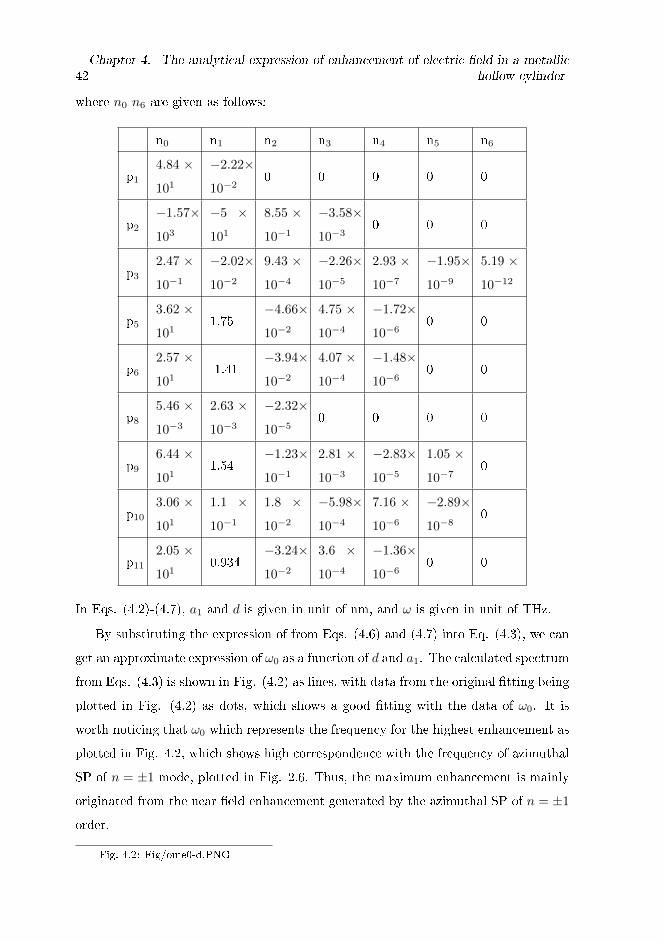
where n0-n6 are given as follows:

n0 n1 n2 n3 n4 n5 n6

p14.84 ×

101

−2.22×

10−20 0 0 0 0

p2−1.57×

103

−5 ×

101

8.55 ×

10−1

−3.58×

10−30 0 0

p32.47 ×

10−1

−2.02×

10−2

9.43 ×

10−4

−2.26×

10−5

2.93 ×

10−7

−1.95×

10−9

5.19 ×

10−12

p53.62 ×

1011.75

−4.66×

10−2

4.75 ×

10−4

−1.72×

10−60 0

p62.57 ×

1011.41

−3.94×

10−2

4.07 ×

10−4

−1.48×

10−60 0

p85.46 ×

10−3

2.63 ×

10−3

−2.32×

10−50 0 0 0

p96.44 ×

1011.54

−1.23×

10−1

2.81 ×

10−3

−2.83×

10−5

1.05 ×

10−70

p103.06 ×

101

1.1 ×

10−1

1.8 ×

10−2

−5.98×

10−4

7.16 ×

10−6

−2.89×

10−80

p112.05 ×

1010.934

−3.24×

10−2

3.6 ×

10−4

−1.36×

10−60 0

In Eqs. (4.2)-(4.7), a1 and d is given in unit of nm, and ω is given in unit of THz.

By substituting the expression of from Eqs. (4.6) and (4.7) into Eq. (4.3), we can

get an approximate expression of ω0 as a function of d and a1. The calculated spectrum

from Eqs. (4.3) is shown in Fig. (4.2) as lines, with data from the original �tting being

plotted in Fig. (4.2) as dots, which shows a good �tting with the data of ω0. It is

worth noticing that ω0 which represents the frequency for the highest enhancement as

plotted in Fig. 4.2, which shows high correspondence with the frequency of azimuthal

SP of n = ±1 mode, plotted in Fig. 2.6. Thus, the maximum enhancement is mainly

originated from the near �eld enhancement generated by the azimuthal SP of n = ±1

order.

Fig. 4.2: Fig/ome0-d.PNG

4.1. The �tting of enhancement spectra 43

Figure 4.2 ω0 as a function of d for di�erent a1. Dots represents the numerical solutioncalculated from Eqs. (2.130) and (2.131), lines represent the �tting of ω0 with exponentialfunction given by Eq. (4.3).

By substituting the expressions we get for ω0, h and γ back in Eq. (4.2), we could

then get an approximate expression of enhancement |E/E0| as a function of ω, a1

and d. In Fig. (4.3), we plot the |E/E0| we calculated from numerical calculation

[calculated from Eqs. (2.130) and (2.131)] and the �tting procedure [Eqs. (4.2) -

(4.5)] in a same �gure. We can observe from Fig. (4.3), that for a given geometry,

the �tting procedure gives an enhancement spectrum close to those calculated from

numerical calculation.

Equation (4.1) provides an analytical expression of enhancement as a function of

incident frequency ω and geometry parameters a1 and d. In the next section, we will

use the obtained analytical expression for obtaining the optimized geometry that gives

the maximum enhancement for a given frequency of incident light.

Fig. 4.3: Fig/peak-compare.PNGFig. 4.4: Fig/optimized.PNG


hollow cylinder

Figure 4.3 |E/E0|'s from numerical calculation are given by the colored dots for severalgeometries while that from analytical expression [Eq. (4.2)] are given by solid lines with thesame color. The geometries of the spectrum was written in the bracket.

Figure 4.4 (a) Optimized thickness dres and (b) Optimized enhancement |E/E0|res plottedas functions of a1 under given resonance frequencies. Blue solid line for ω0 = 3000 THz,orange dash line for ω0 = 3500 THz, green dot dash line for ω0 = 4000 THz. Vertical linesrepresent the critical geometries a1 = acrit1 of the corresponding spectrum.

4.2. Optimized geometry 45

4.2 Optimized geometry

In this section we try to �nd the possible geometry value range for �eld enhancement

peak to exist, and the way to �nd the optimized geometry if the incident light frequency

is given.

Resonant frequency as depicted in Fig. 4.2 decreases as d increase, which means

for a given a1, there would be an upper limit of ω0. When d → ∞ in Eq. (4.3), we

will get the upper limit of frequency ω[sat] for a given inner radius a1:

ω[sat](a1) = 4.84× 101 − 2.22× 10−2a1. (4.8)

ω[sat] determines the saturated value of resonance frequency ω0 as d ≈ ∞ for a given

inner radius a1, when ω0 > ω[sat], the peak enhancement caused by azimuthal SP in a

cylinder will not occur, no matter what value of the thickness d is.

More importantly, from Eq. (4.8) we can also get the expression of critical geometry

a[sat]1 to get resonance condition for a given incident light frequency ω, which is written

as follows:

a[up]1 = 2.18× 103 − 4.5× 101ω, (4.9)

Equation (4.9) determines the upper limit of a1 for getting the resonance condition

for a given incident light frequency ω.

Now we want to present an expression of the optimized parameters. For a given

incident light frequency ω, the resonant condition requires ω = ω0. By using Eq. (4.3),

we can get an expression of optimized d as function of a1 for any given ω = ω0:

dres =ln (ω0 − p1(a1))− ln p2(a1)

p3(a1). (4.10)

By substituting d = dres into Eq. (4.4), we get the optimized enhancement |E/E0|optas a function of a1 for a given ω0 as follows:

|E/E0|opt =p4(a1)

1 + ( ln (ω0−p1(a1))−ln p2(a1)−p3(a1)p5(a1)p3(a1)p6(a1)

)2+ p7(a1)e

−p8(a1) ln (ω0−p1(a1))−ln p2(a1)

p3(a1) .

(4.11)

In Fig. 4.4, we plot dres and |E/E0|opt to a1 for several given ω0. We �nd that, in

consistence with the result given in Sec. 3.1 the enhancement is generally very large


hollow cylinder

(more than 14 times) with very small a1 and d, which coincides the result shown in Fig.

3.3. Another region of signi�cant optimized enhancement is when a1 → a[up]1 , d ≈ 60

nm. Eqs. (4.10) and (4.11) can be used to �nd the optimized geometry parameters of

the metallic hollow cylinder when the incident light frequency is determined.

Chapter 5

Conclusions

In this thesis, we present the study of the electric �eld enhancement generated by

surface electromagnetic (EM) modes in a metallic hollow cylinder. A surface plasmon

(SP) mode has a mathematical structure of a surface TM mode. There are two types

of surface TM modes on a hollow cylinder, one type propagates along the axis of the

cylinder, i.e an axial SP, while another type oscillates around the circumference, i.e.

and azimuthal SP. We inspect the case of a cylinder with a dielectric core in vacuum.

The axial SP cannot be excited by a light in vacuum, while an azimuthal SP can be

excited by shading a light to the cylinder. From the numerical simulation we �nd

that the excited azimuthal SP yields a strong electric �eld enhancement inside the

cylinder. We �nd that such enhancement is generated mainly by the azimuthal SP

mode of n = ±1 order. Such strong enhancement would enhance light absorption rate

inside the cylinder.

We then try to provide analytical relation between radii of the cylinder, incident

frequency and the enhancement, so that we can use such mathematical relation to

�nd out the optimized structure to generate strongest near �eld enhancement inside

the cylinder for any incident light with a given frequency, or vise versa. We �nds

that the enhancement spectrum can be represented as a Lorentzian function as a

function of frequency ω, while the parameters of this Lorentzian function determines

the optimized enhancement and the resonance frequency. The expression of these

parameters of Lorentzian function was �tted as a function of geometry parameters a1

and d, from which we obtain the critical geometry and critical frequency to generate

47

48 Chapter 5. Conclusions

azimuthal SP, and then we obtain the optimized geomtery for a given frequency of the

incident light.

Appendix A

Calculation Programs

Most of the calculation in this thesis is done analytically. Beside �tting and the

plotting, the numerical calculation was mainly used for the calculation of the dispersion

and the calculation of the enhancement, in both situations, the major job is the solving

of either an 8× 8 matrix equation or a 4× 4 matrix equations which is the simpli�ed

version of the previous equation. The core part of most of the programs we presents

here are essentially the same.

All the necessary programs can be found under the following directory in FLEX

workstation.

tian/python/cylinder

A.1 Dispersion for axial surface plasmon in hollow cylinder

Program: hollowaxial.py

Inputs:

Geometry parameters a1 and a2 and index n can be changed.

Outputs:

The dispersion relation is plotted and saved as �le dispersionaxial.jpg

49

50 Appendix A. Calculation Programs

A.2 Dispersion and the enhancement for azimuthal surface

plasmon in hollow cylinder

Program: nmmodes.py

Inputs:

Geometry parameters a1 and a2 and index n can be changed, The data range ran

for 2d spacial plot of the enhancement can be changed to �t the diameter.

Outputs:

The dispersion relation is plotted and saved as �le dispersionazimuthal.jpg, 2d

spacial plot of the enhancement is saved as �le '2denhancement.jpg'. The plot of

the enhancement along x-axis and y-axis is saved in �les 1denhancementx.jpg and

1denhancementy.jpg, repsectively.

A.3 Enhancement spectrum and the �tting

Program: azimuthalfitting.py

Inputs:

Geometry parameters a1 and d, the �tting range omerange and initial guess of the

�tting function.

Output:

The parameters w0, gam and g of the Lorentzian �tting function, which will be

printed on screen and in output.txt, the numerically calculated spectrum of the en-

hancement and the enhancement plotted from the �tting Lorentzian function would

be printed as �le azi�t.jpg, with the derivation of the �tting shown on the �gure. After

every �tting operator should check the accuracy of the �tting, and decide whether to

collect the data or discard it.

Presentation list

Oral presentations

1. Y. Tian, M. S. Ukhtary, R. Saito: Enhancement of electric �eld by surface

plasmon on hollow cylinder. Presented in ATI 2019 Nano-Carbon Meeting and

Zao19 Meeting (2019.8.8-9), Yamagata-Zao, Japan.

Poster Presentations

1. Y. Tian, F. R. Pratama, M. S. Ukhtary, R. Saito: The enhancement of the

electric �eld around the metallic cylindrical tube. Presented in 56th Fullerene-

Nanotubes-Graphene General Symposium of Nanotubes (2019.3.2-4), Tokyo,

Japan.

2. Y. Tian, M. S. Ukhtary, R. Saito: Enhancement of electric �eld by surface

plasmon on hollow cylinder. Presented in 57th Fullerene-Nanotubes-Graphene

General Symposium of Nanotubes (2019.9.3-5), Nagoya Japan.

51

Bibliography

[1] F R Pratama, M Shou�e Ukhtary, and Riichiro Saito, Condens. Matter 31 265701

31, 265701 (2019).

[2] Ryan Beams, Journal of Raman Spectroscopy 49(1), 157�167 (2018).

[3] Bruno Pettinger. Tip-enhanced Raman spectroscopy (TERS). In Surface-

Enhanced Raman Scattering, pages 217�240, Springer, 2006.

[4] Nicolas Guillot, Hb Shen, B Frémaux, Olivier Péron, Emmanuel Rinnert, Timo-

thée Toury, and M Lamy de la Chapelle, Applied Physics Letters 97(2), 023113

(2010).

[5] F Keilmann, Journal of microscopy 194(2-3), 567�570 (1999).

[6] AE Kryukov, Y-K Kim, and John B Ketterson, Journal of applied physics 82(11),

5411�5415 (1997).

[7] Kristofer Tvingstedt, Nils-Krister Persson, Olle Inganäs, Aliaksandr Rahachou,

and Igor V Zozoulenko, Applied Physics Letters 91(11), 113514 (2007).

[8] Kui Bao Ulf H?kanson Naomi J. Halas PeterNordlander Shunping Zhang,

Hong Wei and Hongxing Xu, 107(9), 096801 (August 2011).

[9] Dror Sarid and William Challener, Modern introduction to surface plasmons:

theory, Mathematica modeling, and applications (Cambridge University Press,

Cambridge, 2010).

[10] J. E. Ingles�eld, Solid State Communications 40, 467�471 (1981).

[11] Mario Rocca, Surface science reports 22(1-2), 1�71 (1995).

53

54 Bibliography

[12] Stefan Alexander Maier, Plasmonics: fundamentals and applications: fundamen-

tals and applications (Springer Science & Business Media, Bath, 2007).

[13] M Shou�e Ukhtary and Riichiro Saito, Carbon (2020).

[14] Anatoly V Zayats and Igor I Smolyaninov, Journal of Optics A: Pure and Applied

Optics 5(4), S16 (2003).

[15] VS Zuev, AV Frantsesson, J Gao, and JG Eden, The Journal of chemical physics

122(21), 214726 (2005).

[16] A Yelon, KN Piyakis, and E Sacher, Surface science 569(1-3), 47�55 (2004).

[17] Ellen J. Zeman and George C. Schatz, Journal of Physical Chemistry, 91, 634�643

(1987).

[18] Alexandre Vial, Anne-Sophie Grimault, Demetrio Macías, Dominique Barchiesi,

and Marc Lamy de la Chapelle, Physical Review B 71(8) (feb 2005).

[19] Anastasiya Derkachova, Krystyna Kolwas, and Iraida Demchenko, Plasmonics 11,

941�951 (2016).

[20] Alexandre Vial, Anne-Sophie Grimault, Demetrio Macas, Dominique Barchiesi,

and Marc Lamy de la Chapelle, Physical Review B 71(8) (feb 2005).

[21] Bo Johnsson, Stefan Löfås, and Gabrielle Lindquist, Analytical biochemistry

198(2), 268�277 (1991).

[22] Eliza Hutter and Janos H Fendler, Advanced materials 16(19), 1685�1706 (2004).

[23] Dajian Wu, Xiaojun Liu, and Bo Li, Journal of Applied Physics 109(8), 083540

(2011).

[24] Barbora �pa£ková, N Scott Lynn, Ji°í Homola, Pavel Kwiecien, and Ivan Richter.

In SENSORS, 2012 IEEE, pages 1�4. IEEE, 2012.

[25] D Taverna, M Kociak, V Charbois, and L Henrard, Physical Review B 66(23),

235419 (2002).

[26] DJ Mowbray, S Segui, J Gervasoni, ZL Mi²kovi¢, and NR Arista, Physical Review

B 82(3), 035405 (2010).

Bibliography 55

[27] Shulin Sun, Hung-Ting Chen, Wei-Jin Zheng, and Guang-Yu Guo, 21, 14591

(2013).

[28] Diego M Solis, Jose Manuel Taboada, Luis Landesa, Jose Luis Rodriguez, and

Fernando Obelleiro, Progress In Electromagnetics Research 154, 35�50 (2015).

[29] Harald Ditlbacher, Andreas Hohenau, Dieter Wagner, Uwe Kreibig, Michael

Rogers, Ferdinand Hofer, Franz R Aussenegg, and Joachim R Krenn, Physical

review letters 95(25), 257403 (2005).

[30] Qian Zhao, Ji Zhou, Fuli Zhang, and Didier Lippens, Materials today 12(12),

60�69 (2009).

[31] R Sainidou and FJ García de Abajo, Optics express 16(7), 4499�4506 (2008).

[32] Ken-ichi Sasaki, Shuichi Murakami, and Hideki Yamamoto, Applied Physics Let-

ters 108(16), 163109 (2016).

[33] Milton Abramowitz, Irene A Stegun, and Robert H Romer. Handbook of math-

ematical functions with formulas, graphs, and mathematical tables, 1988.

[34] Craig F Bohren and Donald R Hu�man, , 2008).

[35] Julius Adams Stratton, Electromagnetic Theory (John Wiley & Sons, Piscataway,

2007).

[36] CA Pfei�er, EN Economou, and KL Ngai, Physical review B 10(8), 3038 (1974).

[37] Ilja N Bronshtein and Konstantin A Semendyayev, Handbook of mathematics

(Springer Science & Business Media, Berlin, 2013).

[38] C Leubner, Physical Review A 23(6), 2877 (1981).

[39] H Hövel, S Fritz, A Hilger, U Kreibig, and Michael Vollmer, Physical Review B

48(24), 18178 (1993).

[40] Kheirandish Asef, Sepehri Javan Nasser, and Mohammadzadeh Hosein, Scienti�c

Reports (Nature Publisher Group) 10(1) (2020).

Date post:	30-Nov-2021
Category:	Documents
Upload:	others
View:	1 times
Download:	0 times

Master Thesis - flex.phys.tohoku.ac.jp

Documents