DEPARTMENT OF TECHNOLOGY AND BUILT ENVIRONMENT Characterization of a 5GHz Modular Radio Frontend for WLAN Based on IEEE 802.11p M ahdi Abbasi Vienna, December 2008 Master’s Thesis in Telecommunications Examiner: Prof. Claes Beckman Supervisors: Ao.Univ.Prof. Univ.Prof. Dipl.-Ing. Dr.techn Arpad L. Scholtz Univ.Prof. Dipl.-Ing. Dr.-Ing. Christoph F. Mecklenbr¨auker Univ.Ass. Dipl.-Ing. Alexander Paier INSTITUT FÜR NACHRICHTENTECHNIK UND HOCHFREQUENZTECHNIK
Transcript
DEPARTMENT OF TECHNOLOGY AND BUILT ENVIRONMENT
Characterization of a 5GHz Modular
Radio Frontend for WLAN Based on
IEEE 802.11p
Mahdi Abbasi
Vienna, December 2008
Master’s Thesis in Telecommunications
Examiner: Prof. Claes Beckman
Supervisors: Ao.Univ.Prof. Univ.Prof. Dipl.-Ing. Dr.techn Arpad L. Scholtz
Univ.Prof. Dipl.-Ing. Dr.-Ing. Christoph F. Mecklenbrauker
The number of vehicles has increased significantly in recent years, which causeshigh density in traffic and further problems like accidents and road congestions.A solution regarding to this problem is vehicle-to-vehicle communication, wherevehicles are able to communicate with their neighboring vehicles even in the ab-sence of a central base station, to provide safer and more efficient roads and toincrease passenger safety.
The goal of this thesis is to investigate basic physical layer parameters of ainter-vehicle communication system, like emission power, spectral emission, errorvector magnitude, guard interval, ramp-up/down time, and third order interceptpoint. I also studied the intelligent transportation system’s channel layout inEurope, how the interference of other systems are working in co-channel and ad-jacent channels, and some proposals to use the allocated frequency bands. On theother hand, the fundamentals of OFDM transmission and definitions of OFDMkey parameters in IEEE 802.11p are investigated.
The focus of this work is on the measurement of transmitter frontend parame-ters of a new testbed designed and fabricated in order to be used at inter-vehiclecommunication based on IEEE 802.11p.
ii
Dedicated to :
My Parents
And to my lovely wife Samaneh
iii
Acknowledgement
This thesis has been carried out at the institute of communications and radio-frequency engineering at the technical university of Vienna, Austria.
I would Like to particularly grateful to Professor Christoph F. Mecklenbraukerand Professor Arpad L. Scholtz for introducing me to the subject and providingcontinuous guidance and support, and giving me the opportunity to develop andwork at this institute. Thanks are extended to Alexander Paier for his kind as-sistance with patience.
I am deeply appreciative of my family for their endless love, care and support.
iv
List of Abbreviations
ACP Adjacent Channel PowerCCH Control ChannelCDF Cumulative Distribution FunctionCP Channel PowerDFS Dynamic Frequency SelectionDSO Digital Storage OscilloscopeDUT Device Under TestECC Electronic Communications CommitteeEVM Error Vector MagnitudeFCC Federal Communications CommissionFS Fixed ServiceFSS Fixed Satellite ServiceFWA Fixed Wireless AccessGI Guard IntervalGPS Global Positioning SystemIFFT Inverse Fast Fourier TransformIP3 Third Order Intercept PointISI Inter-Symbol InterferenceISM Industrial, Scientific and Medical bandITS Intelligent Transportation SystemIVC Inter-Vehicle CommunicationLCR Level Crossing RateLOS Line of SightNLOS Non Line of SightOBU On Board UnitOFDM Orthogonal Frequency Division MultiplexingOoB Out of BandPDF Probability Density FunctionPHY Physical layerPSD Power Spectral DensityR2V Roadside-to-Vehicle CommunicationRBW Resolution BandwidthRL RadiolocationRMS Root Mean SquareSRD Short-Range DevicesRSU Road Side UnitRTTT Road Transport and Traffic Telematics
v
SCH Service ChannelsTDMA Time Division Multiple AccessV2I Vehicle-to-Infrastructure CommunicationV2V Vehicle-to-Vehicle CommunicationVSA Vector Signal AnalyzerVSG Vector Signal GeneratorWAVE Wireless Access in Vehicular EnvironmentsWLAN Wireless Local Area Network
Road accidents take the life of many people in the world each year, and much morepeople have been injuring and maiming. Statistical studies show that accidentscould be shunned by 60 % if drivers be informed only half a second before theaccident, [1]. The main reason of these accidents is a limitation in view of roadwayemergency events that can be due to the distances, darkness, and existence of aninhibiter in the road (a vehicle, building, rock, etc). Also a delay of the vehicle’sdriver to react against the events on the roadway could make irreparable results,[2].
Communication between vehicles, Vehicle-to-Vehicle (V2V), and between avehicle and an immobile access point, Vehicle-to-Infrastructure (V2I), have thepotential to contribute considerably to the elimination of traffic accidents. V2Vand V2I communications (called V2X) could be profitable in traffic congestiondecreasing. The concept of this communication is to send safety messages by avehicle to many other vehicles via wireless connection. In this technology, vehiclescan communicate and collaborate with each other, exchanging both safety andnon-safety information. Therefore commercial benefits can be mentioned in thiscommunication too.
A very promising specification for vehicular communications is the draft stan-dard IEEE 802.11p, [3], also known as Wireless Access in Vehicular Environments(WAVE). This specification is an advancement of the well-known Wireless LocalArea Network (WLAN) standard IEEE 802.11, [4], which operates in the 5.9 GHzfrequency band and is conceived for data communication in traffic scenarios withspeeds up to 72 m/s.
In the IEEE 802.11p standard, communication signals are generated with theOrthogonal Frequency Division Multiplexing (OFDM) technique principle. Thiswork describes fundamentals of OFDM transmission as well as front-end char-acterization such as emission power, spectral emission, Error Vector Magnitude(EVM), Guard Intervals (GI), ramp up/down time and 3rd order Intercept Point(IP3) in chapter 2. All these subjects are under investigation to use in V2Xcommunications.
In this thesis I investigate a transceiver, which has implemented the draftstandard IEEE 802.11p. OFDM parameters and Physical layer (PHY) signals ofthe transceiver must meet the specifications defined in the standard. This device
1
Contents
named ”RouterBOARD 532A” is developed by Siemens AG Austria and has twoantennas for transmitting and receiving the signals.
Finally the measurements on the transceiver, for the desired parameters will beexplained in chapter 4. Measuring the Front-end characterization of transmitterlike emission part, specrum mask, error vector magnitude, and ramp-up/downtime are categorized in the practical part of the thesis. All these specificationswill be compared with the IEEE 802.11p standard.
2
Chapter 2
Introduction
In this chapter, fundamentals of an OFDM transmission are introduced and someimportant parts creating an OFDM signal, such as Inverse Fast Fourier Trans-form (IFFT), cyclic prefix and the effect of subcarrier amount on the spectrumof an OFDM signal, are explained in detail. Afterward the fundamental param-eters of frontend characterization are discussed. In section 2.3 the importance ofdynamics of vehicular wireless channels are clarified and explained in detail.
2.1 Fundamentals of OFDM Transmission
The draft standard IEEE 802.11p is based on OFDM transmission technology.Therefore a higher spectral efficiency, lower sensitivity in synchronization errorsand less Inter-Symbol Interference (ISI) could be expected, compared to the othertechniques like Time Division Multiple Access (TDMA). In an OFDM signal, ahigher data bit rate channel is divided into multiple orthogonal sub-channelsin the frequency domain with lower bit rates. By this multiplexing technique,there exist several narrow-band subcarriers instead of a wide band carrier. Thisconversion is shown clearly in Figure 2.1. In the first part of the figure, threesymbols A, B, and C are included in a signal with a specific frequency andseparated in time. In the second part of the Figure 2.1 these symbols are extendedin time, but separated in carrier’s frequency, so the probability of wasting asymbol due to multipath propagation of the signal is reduced, because in thenew situation, the symbols have less overlap on the adjacent symbols. A morecomplete description of an OFDM signal can be seen in Figure 2.2. As Figure2.2 shows, an OFDM signal is divided in both time and frequency domain andso increases the capacity of the system in addition to the less interference of theadjacent symbols. The guard interval between the symbols in time domain isshown also in the Figure 2.2. More detail explanation about guard interval inOFDM signal is explained in Section 2.1.2.
2.1.1 IFFT
To create the OFDM symbol in practice, a serial to parallel chip is used in orderto convert a signal with N serial symbols to a signal with N parallel symbols.
3
2.1 Fundamentals of OFDM Transmission
t
f
Symbol A Symbol B Symbol C
Symbol Time
T
t
f1
Symbol A
t
Symbol B
t
f3
Symbol C
Symbol Time
Tprime
Single Carrier
Multi Carrier
f2
Figure 2.1: Single carrier comparison with multi carrier.
Frequency
Am
plit
ud
e
Time
Guard
Interval
Symbol
Figure 2.2: OFDM time/frequency representation.
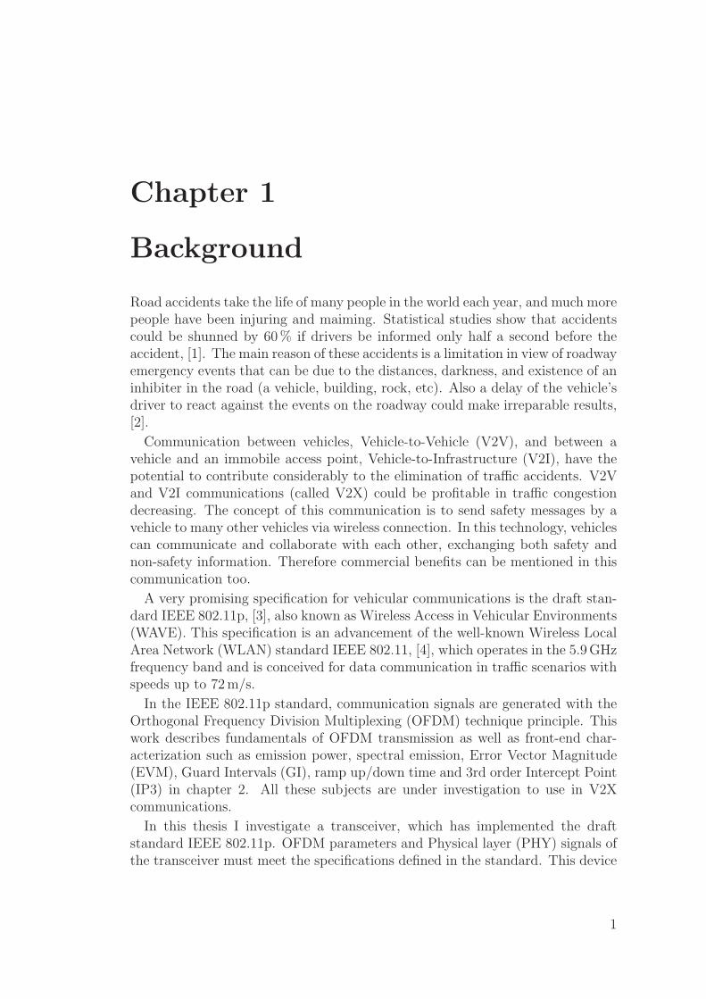
Each parallel data symbol (orthogonal sub-carrier) is modulated and then themodulated subcarriers are added together. because of practical reasons, thisprocedure is implemented by an IFFT block. Figure 2.3 shows a simple blockdiagram of an IFFT system.
2.1.2 Cyclic Prefix Insertion
Wireless communications systems are predisposed to multi-path propagation onthe radio channel. Adding a cyclic prefix to the signal reduces the ISI. The
4
2.2 Fundamentals of Frontend Characterization
Serial
to
Parallel
IFFT
Figure 2.3: IFFT.
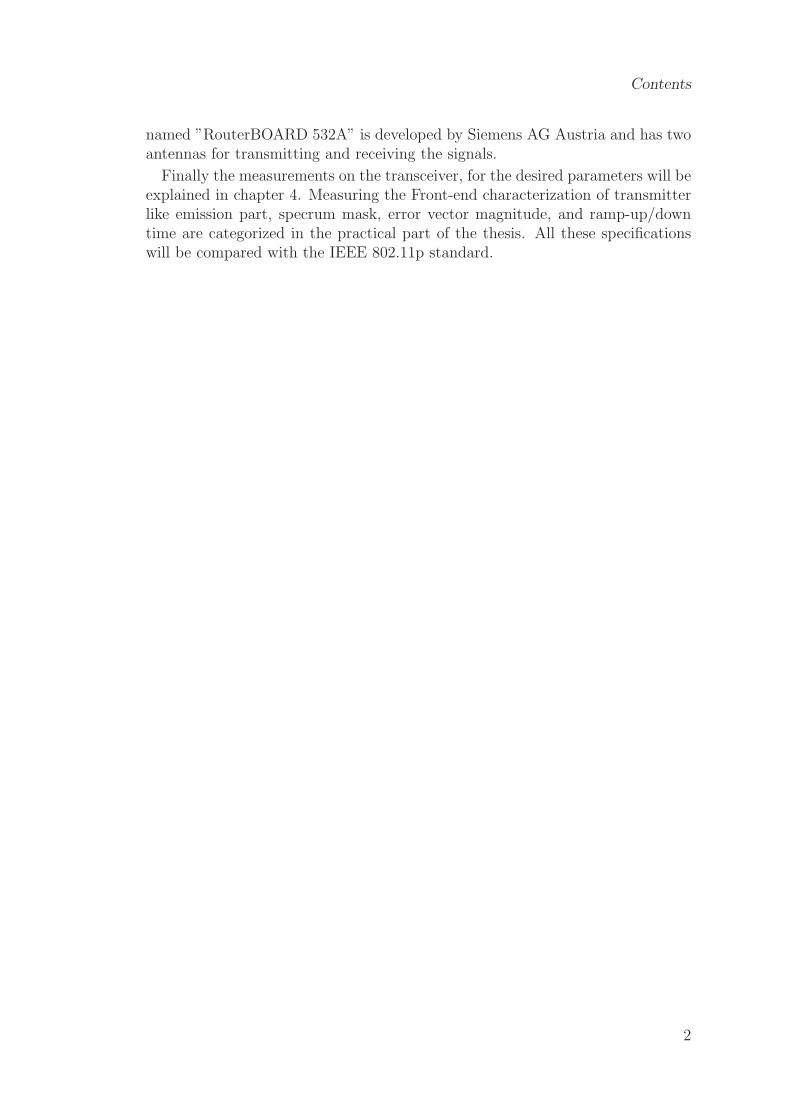
cyclic prefix is repetition of the last part of a symbol at the beginning of thesame symbol that is illustrated in Figure 2.4. Multi-path propagation causesthe original signal to fade, so a guard interval in the symbol will improve thetransmission. The cyclic prefix technique is being used as a guard interval inthe OFDM signals. In the presence of a cyclic prefix, interference signals do notinterfere with the main part of the symbol, [5].
time
Symbol 2Symbol 1
GI Symbol Period GI Symbol Period
Figure 2.4: Cyclic Prefix Insertion.
2.1.3 OFDM Spectrum
A number of sub-carriers, k, of an OFDM signal with the same bandwidth isaffecting the power level of the side-lobes in the power density spectrum. Afaster side-lobe decay is due to a larger amount of the K. Spectrum mask ofIEEE 802.11p is described in detail in Section 2.2.1. The spectrum mask inIEEE 802.11p is divided into 64 sub-carriers.
2.2 Fundamentals of Frontend Characterization
2.2.1 Emission Power and Spectral Emission
The transmit spectrum mask specifies the power limitation in a specific frequencybandwidth and a certain offsets relative to the maximum carrier power, therefore
5
2.2 Fundamentals of Frontend Characterization
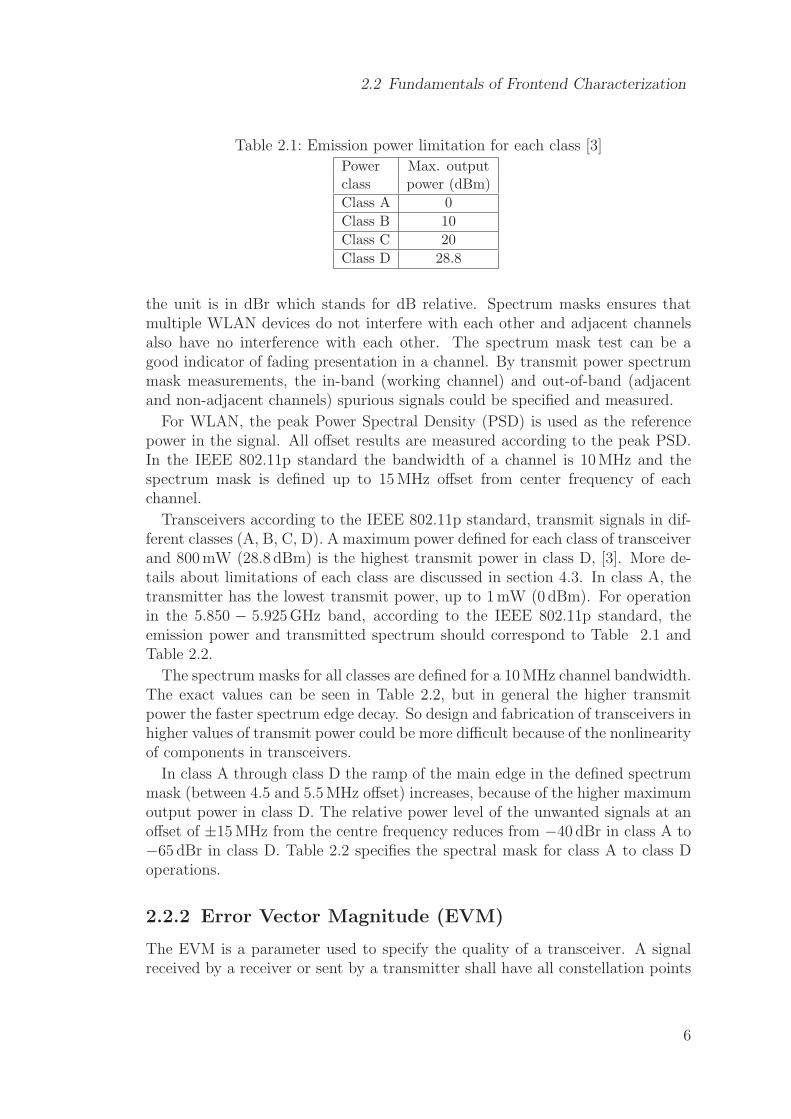
Table 2.1: Emission power limitation for each class [3]
Power Max. outputclass power (dBm)
Class A 0
Class B 10
Class C 20
Class D 28.8
the unit is in dBr which stands for dB relative. Spectrum masks ensures thatmultiple WLAN devices do not interfere with each other and adjacent channelsalso have no interference with each other. The spectrum mask test can be agood indicator of fading presentation in a channel. By transmit power spectrummask measurements, the in-band (working channel) and out-of-band (adjacentand non-adjacent channels) spurious signals could be specified and measured.
For WLAN, the peak Power Spectral Density (PSD) is used as the referencepower in the signal. All offset results are measured according to the peak PSD.In the IEEE 802.11p standard the bandwidth of a channel is 10 MHz and thespectrum mask is defined up to 15 MHz offset from center frequency of eachchannel.
Transceivers according to the IEEE 802.11p standard, transmit signals in dif-ferent classes (A, B, C, D). A maximum power defined for each class of transceiverand 800 mW (28.8 dBm) is the highest transmit power in class D, [3]. More de-tails about limitations of each class are discussed in section 4.3. In class A, thetransmitter has the lowest transmit power, up to 1 mW (0 dBm). For operationin the 5.850 − 5.925 GHz band, according to the IEEE 802.11p standard, theemission power and transmitted spectrum should correspond to Table 2.1 andTable 2.2.
The spectrum masks for all classes are defined for a 10 MHz channel bandwidth.The exact values can be seen in Table 2.2, but in general the higher transmitpower the faster spectrum edge decay. So design and fabrication of transceivers inhigher values of transmit power could be more difficult because of the nonlinearityof components in transceivers.
In class A through class D the ramp of the main edge in the defined spectrummask (between 4.5 and 5.5 MHz offset) increases, because of the higher maximumoutput power in class D. The relative power level of the unwanted signals at anoffset of ±15 MHz from the centre frequency reduces from −40 dBr in class A to−65 dBr in class D. Table 2.2 specifies the spectral mask for class A to class Doperations.
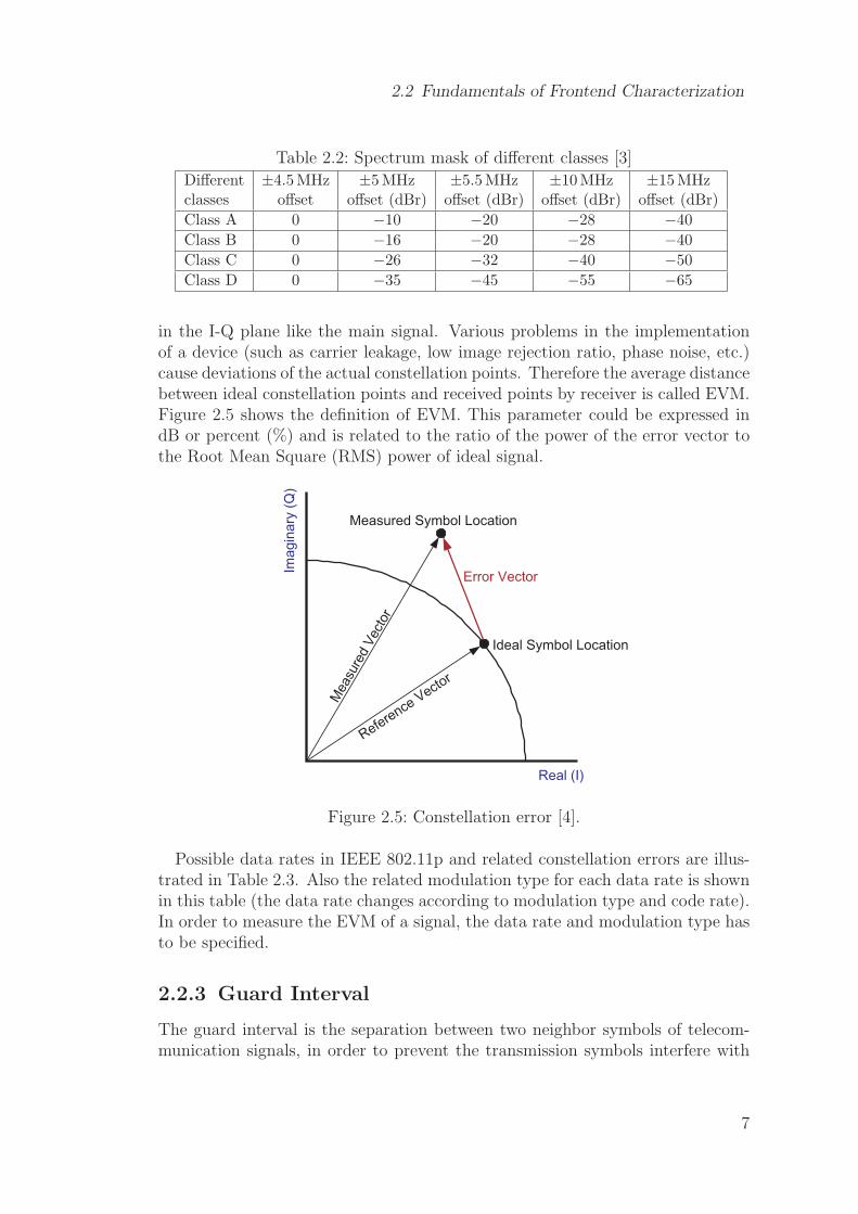
2.2.2 Error Vector Magnitude (EVM)
The EVM is a parameter used to specify the quality of a transceiver. A signalreceived by a receiver or sent by a transmitter shall have all constellation points
in the I-Q plane like the main signal. Various problems in the implementationof a device (such as carrier leakage, low image rejection ratio, phase noise, etc.)cause deviations of the actual constellation points. Therefore the average distancebetween ideal constellation points and received points by receiver is called EVM.Figure 2.5 shows the definition of EVM. This parameter could be expressed indB or percent (%) and is related to the ratio of the power of the error vector tothe Root Mean Square (RMS) power of ideal signal.
Ima
gin
ary
(Q)
Real (I)
Reference Vecto
r
Measu
red
Vect
or
Measured Symbol Location
Ideal Symbol Location
Error Vector
Figure 2.5: Constellation error [4].
Possible data rates in IEEE 802.11p and related constellation errors are illus-trated in Table 2.3. Also the related modulation type for each data rate is shownin this table (the data rate changes according to modulation type and code rate).In order to measure the EVM of a signal, the data rate and modulation type hasto be specified.
2.2.3 Guard Interval
The guard interval is the separation between two neighbor symbols of telecom-munication signals, in order to prevent the transmission symbols interfere with
7
2.2 Fundamentals of Frontend Characterization
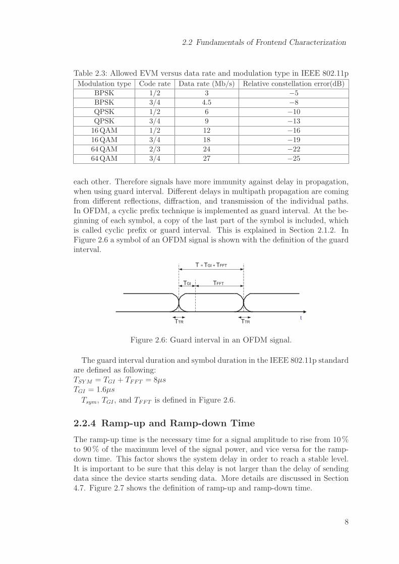
Table 2.3: Allowed EVM versus data rate and modulation type in IEEE 802.11p
Modulation type Code rate Data rate (Mb/s) Relative constellation error(dB)
BPSK 1/2 3 −5
BPSK 3/4 4.5 −8
QPSK 1/2 6 −10
QPSK 3/4 9 −13
16 QAM 1/2 12 −16
16 QAM 3/4 18 −19
64 QAM 2/3 24 −22
64 QAM 3/4 27 −25
each other. Therefore signals have more immunity against delay in propagation,when using guard interval. Different delays in multipath propagation are comingfrom different reflections, diffraction, and transmission of the individual paths.In OFDM, a cyclic prefix technique is implemented as guard interval. At the be-ginning of each symbol, a copy of the last part of the symbol is included, whichis called cyclic prefix or guard interval. This is explained in Section 2.1.2. InFigure 2.6 a symbol of an OFDM signal is shown with the definition of the guardinterval.
TGI TFFT
TTR
T = TGI + TFFT
TTRt
Figure 2.6: Guard interval in an OFDM signal.
The guard interval duration and symbol duration in the IEEE 802.11p standardare defined as following:TSY M = TGI + TFFT = 8µsTGI = 1.6µs
Tsym, TGI , and TFFT is defined in Figure 2.6.
2.2.4 Ramp-up and Ramp-down Time
The ramp-up time is the necessary time for a signal amplitude to rise from 10 %to 90 % of the maximum level of the signal power, and vice versa for the ramp-down time. This factor shows the system delay in order to reach a stable level.It is important to be sure that this delay is not larger than the delay of sendingdata since the device starts sending data. More details are discussed in Section4.7. Figure 2.7 shows the definition of ramp-up and ramp-down time.
8
2.2 Fundamentals of Frontend Characterization
Time
Txp
ow
er
Time
Txp
ow
er
Max Tx power Max Tx power
90% Max
10% Max
90% Max
10% Max
Figure 2.7: Transmit power on/down ramp.
2.2.5 Third Order Intercept Point (IP3)
The Third Order Intercept Point (IP3) is a factor to measure the nonlinearity ofsystems and devices. The intercept point is a mathematical concept, and doesnot correspond to a practically occurring physical power level. The nth orderintermodulation products appear at n times the frequency spacing of the inputtones. Figure 2.8 shows the intermodulation products of a two tone signal. Thirdorder intermodulation products are more important than other intermodulationproducts due to the high relative power level and less distance to main tones.
Frequency
Po
ut
Fundamentals
3rd3rd
5th5th
2nd2nd
f1 f23f1 – 2.f2
2f1-f2 2f2-f1
3f2-2f1
f1+f2f2-f1
Figure 2.8: Intermodulation products.
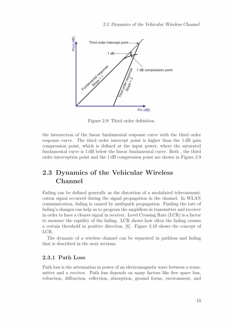
The output power versus the input power, both in logarithmic scale, are shownin Figure 2.9. One curve belongs to the fundamental response of an input signaland is linearly amplified, and the other curve shows the third order intermodu-lation product’s response, which is nonlinearly amplified (with slope 3 ).
The nonlinearity of amplifiers, implemented in transceivers, leads to a 3 dBincrease in third order products when the input power is increased only by 1 dB.Therefore a limitation for amplifier’s input power is required in order to preventdisappearing of the main signal. The third order intercept point is defined at
9
2.3 Dynamics of the Vehicular Wireless Channel
Po
ut
(dB
)
Pin (dB)
Third order intercept point
Third
ord
er
resp
onse
Slo
pe
=3
Funda
men
tal r
espo
nse
Slope
=1
1 dB compression point
1 dB
Figure 2.9: Third order definition.
the intersection of the linear fundamental response curve with the third orderresponse curve. The third order intercept point is higher than the 1 dB gaincompression point, which is defined at the input power, where the saturatedfundamental curve is 1 dB below the linear fundamental curve. Both , the thirdorder interception point and the 1 dB compression point are shown in Figure 2.9
2.3 Dynamics of the Vehicular Wireless
Channel
Fading can be defined generally as the distortion of a modulated telecommuni-cation signal occurred during the signal propagation in the channel. In WLANcommunication, fading is caused by multipath propagation. Finding the rate offading’s changes can help us to program the amplifiers in transmitter and receiverin order to have a clearer signal in receiver. Level Crossing Rate (LCR) is a factorto measure the rapidity of the fading. LCR shows how often the fading crossesa certain threshold in positive direction, [6]. Figure 2.10 shows the concept ofLCR.
The dynamic of a wireless channel can be separated in pathloss and fadingthat is described in the next sections.
2.3.1 Path Loss
Path loss is the attenuation in power of an electromagnetic wave between a trans-mitter and a receiver. Path loss depends on many factors like free space loss,refraction, diffraction, reflection, absorption, ground forms, environment, and
10
2.3 Dynamics of the Vehicular Wireless Channel
Po
we
rre
sp
on
se
(dB
)
Frequency
Level crossing
Threshold
Figure 2.10: Level Crossing Rate (LCR).
propagation medium. In V2V communication, a Line of Sight (LOS) path existsif no blockage is between the transmitter vehicle and receiver vehicle. Accordingto the existence of LOS, different characteristic are defined for path loss. Thepath loss can be investigated in different scenarios like highway, urban and ruralroads, where some factors are different in each scenario, like speed and trafficcongestion.
hrht
rd
rr
Figure 2.11: Two ray path loss model.
For the LOS case one approach is the two ray path loss model for determiningthe received signal power level, described in [7].
Pr =PtGtGr
L(rd)
[
Dd
(
λ
4πrd
)
+ Dr
(
λ
4πrr
)
ηe−j{k(rd−rr)+φ}
]2
(2.1)
Pt is the Txpower, Gt and Gr are the gains of the antennas at transmitterand receiver, alternatively, λ is the propagating signal’s wavelength, rd and rr
are the path lengths of the direct and reflected signals, see Figure 2.11. φ is thephase rotation due to ground reflection, η is the reflection coefficient, Dd andDr are the antenna directivity’s coefficients, L(rd ) is the the factor regarding tothe absorption.
Two scenario can be defined in path loss study, LOS propagation and Non Lineof Side (NLOS) propagation. The NLOS case happens when obstacle appear in
11
2.3 Dynamics of the Vehicular Wireless Channel
between the transmitter antenna and receiver antenna. This scenario happenswhen there is heavy traffic or the communication distance is large. In this casea LOS path may exist only among the adjacent vehicles. One possibility tomodel the path loss in NLOS scenario is the log-distance model with an exponentbetween 2.8 − 5.9 GHz, [7].
Pr = PtGtGr
(
λ
4π
)2
d ≤ 1m (2.2)
Pr = PtGtGr
(
λ
4π
)21
dγd > 1m (2.3)
Where d is the distance between the transmitter and the receiver, and γ takesvalue from 2.8 to 5.9, [7].
2.3.2 Fading
The variation of the amplitude and/or relative phase in a received signal canbe defined as fading. Therefore fading can be described as the variation of thecharacteristics of the propagation path over time or location. Small scale fadingdescribes the oscillation of the received signal strength over very short time du-ration or a short distance. Rician and Rayleigh fading are often used for smallscale fading. Large scale fading is caused by shadowing. The mobile station hasto move over a large distance to remove the effects of shadowing. For shadowingthe log normal distribution is often used, [8].
Rician Fading
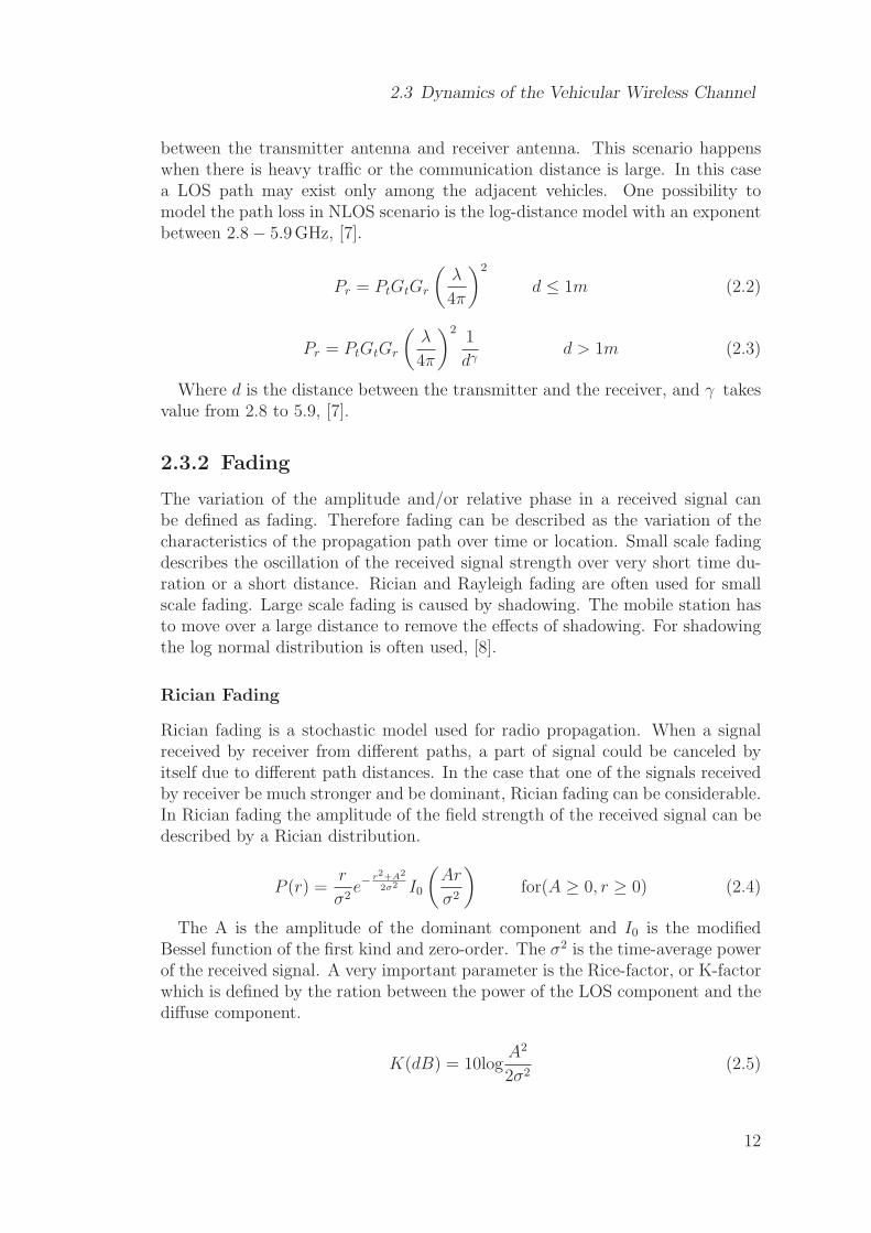
Rician fading is a stochastic model used for radio propagation. When a signalreceived by receiver from different paths, a part of signal could be canceled byitself due to different path distances. In the case that one of the signals receivedby receiver be much stronger and be dominant, Rician fading can be considerable.In Rician fading the amplitude of the field strength of the received signal can bedescribed by a Rician distribution.
P (r) =r
σ2e−
r2+A
2
2σ2 I0
(
Ar
σ2
)
for(A ≥ 0, r ≥ 0) (2.4)
The A is the amplitude of the dominant component and I0 is the modifiedBessel function of the first kind and zero-order. The σ2 is the time-average powerof the received signal. A very important parameter is the Rice-factor, or K-factorwhich is defined by the ration between the power of the LOS component and thediffuse component.
K(dB) = 10logA2
2σ2(2.5)
12
2.3 Dynamics of the Vehicular Wireless Channel
Figure 2.12: Rician and Rayleigh Probability Density Function (pdf).
For K >> 1 the Rician distribution can be approximated by a Gaussian dis-tribution. One example of a Rician distribution is shown in Figure 2.12.
Rayleigh Fading
Rayleigh fading is a kind of Rician fading when K → 0 which means that thereexists no dominant path. Rayleigh fading happens if a signal goes through achannel and the amplitude of the field strength of the signal varies or fades ac-cording to the Rayleigh distribution model. The Rayleigh distribution is definedas
p(r) =
{
rσ2 exp
(
− r2
2σ2
)
(0 ≤ r ≤ ∞)
0 (r < 0)(2.6)
where σ2 is the time-average power of the received signal.
The Cumulative Distribution Function (CDF) is defined in order to specify theprobability that the received signal does not exceed a specific level R.
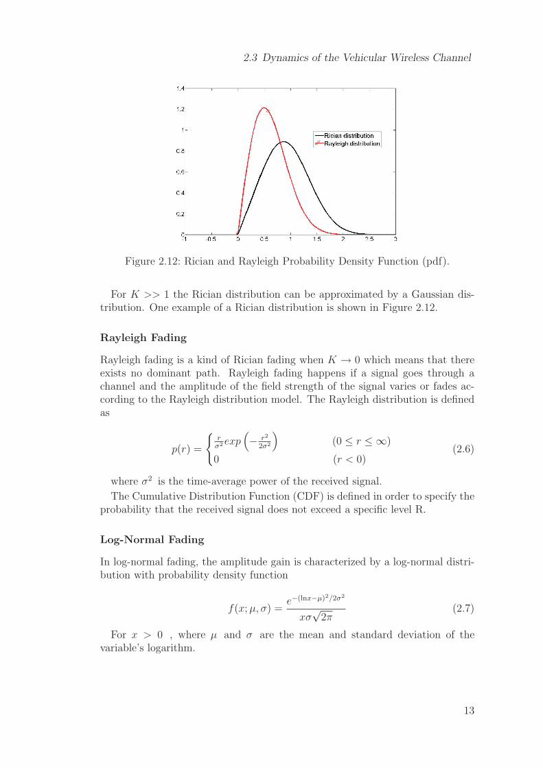
Log-Normal Fading
In log-normal fading, the amplitude gain is characterized by a log-normal distri-bution with probability density function
f(x; µ, σ) =e−(lnx−µ)2/2σ2
xσ√
2π(2.7)
For x > 0 , where µ and σ are the mean and standard deviation of thevariable’s logarithm.
13
2.3 Dynamics of the Vehicular Wireless Channel
0 3 6 9 120
0.5
1
1.5
2
2.5
3
3.5x 10
−5
Figure 2.13: Log-normal distribution.
14
Chapter 3
Wireless LAN According toIEEE 802.11p
3.1 Definition of Key OFDM Parameters
The OFDM technique divides a signal with high data rate into several parallelsignals with lower data rates which are transmitted over orthogonal frequencysubcarriers.
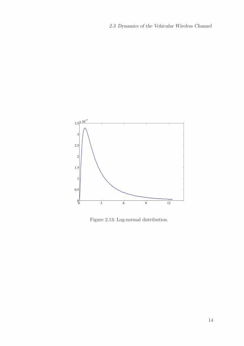
The PHY of the standard IEEE 802.11a is using the OFDM technique with64 subcarriers, [9], (the IEEE 802.11p standard is based on IEEE 802.11a). 52subcarriers out of 64 are used for actual transmission, where 48 are data subcar-riers and 4 are pilot subcarriers. The pilot subcarriers are used for tracing thefrequency offset and phase noise. The PHY data packet structure is illustrated inFigure 3.1. This structure is the same for IEEE 802.11a and IEEE 802.11p. Theshort training symbols, which are located at the beginning of every PHY datapacket, are used for signal detection, coarse frequency offset estimation and timesynchronization. The long training symbols, which are located after the shorttraining symbols, are used for channel estimation and synchronization reasons.A guard interval time GI, i.e. cyclic prefix, is located in the OFDM data packet,in order to remove the ISI caused by the multipath propagation. GI decreasesthe system capacity and so the received effective signal to interference and noiseratio.
GI2 T1 T2 GI Data1GISignalData2
GIt1 t2 t3 t4 t5 t6 t7 t8 t9 t10
Short training
symbolsSignal Detection
Diversity Selection
Long training
symbolsChannel and Fine
Frequency offset
Estimation
Signal symbolRATE
LENGTH
Data
PreambleT=TGI+TFFT
Figure 3.1: packet structure.
15
3.2 Definition of European 5.8 GHz Channel Layout
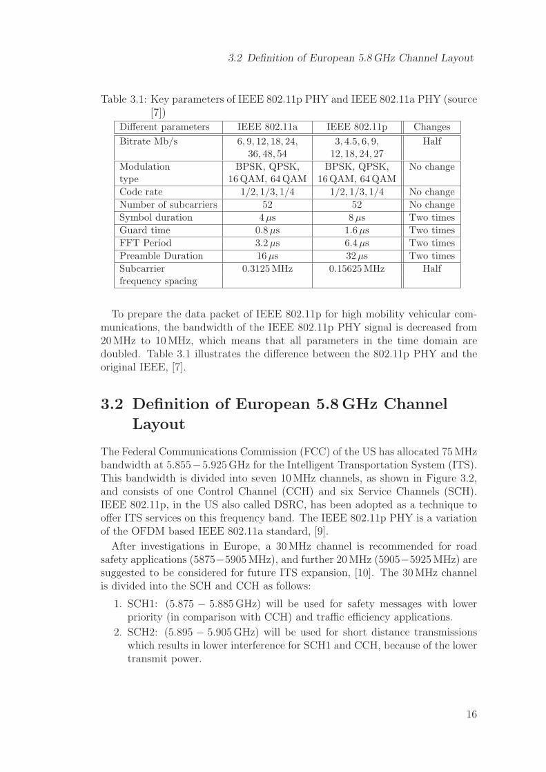
Table 3.1: Key parameters of IEEE 802.11p PHY and IEEE 802.11a PHY (source[7])
Different parameters IEEE 802.11a IEEE 802.11p Changes
To prepare the data packet of IEEE 802.11p for high mobility vehicular com-munications, the bandwidth of the IEEE 802.11p PHY signal is decreased from20 MHz to 10 MHz, which means that all parameters in the time domain aredoubled. Table 3.1 illustrates the difference between the 802.11p PHY and theoriginal IEEE, [7].
3.2 Definition of European 5.8 GHz Channel
Layout
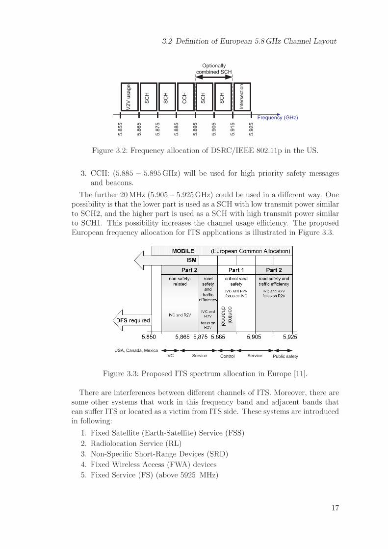
The Federal Communications Commission (FCC) of the US has allocated 75 MHzbandwidth at 5.855−5.925 GHz for the Intelligent Transportation System (ITS).This bandwidth is divided into seven 10 MHz channels, as shown in Figure 3.2,and consists of one Control Channel (CCH) and six Service Channels (SCH).IEEE 802.11p, in the US also called DSRC, has been adopted as a technique tooffer ITS services on this frequency band. The IEEE 802.11p PHY is a variationof the OFDM based IEEE 802.11a standard, [9].
After investigations in Europe, a 30 MHz channel is recommended for roadsafety applications (5875−5905 MHz), and further 20 MHz (5905−5925 MHz) aresuggested to be considered for future ITS expansion, [10]. The 30MHz channelis divided into the SCH and CCH as follows:
1. SCH1: (5.875 − 5.885 GHz) will be used for safety messages with lowerpriority (in comparison with CCH) and traffic efficiency applications.
2. SCH2: (5.895 − 5.905 GHz) will be used for short distance transmissionswhich results in lower interference for SCH1 and CCH, because of the lowertransmit power.
16
3.2 Definition of European 5.8 GHz Channel Layout
Frequency (GHz)5
.85
5
5.8
65
5.8
75
5.8
85
5.8
95
5.9
05
5.9
15
5.9
25
V2
Vu
sa
ge
SC
H
CC
H
Inte
rsection
SC
H
SC
H
SC
H
Optionally
combined SCH
Figure 3.2: Frequency allocation of DSRC/IEEE 802.11p in the US.
3. CCH: (5.885 − 5.895 GHz) will be used for high priority safety messagesand beacons.
The further 20 MHz (5.905− 5.925 GHz) could be used in a different way. Onepossibility is that the lower part is used as a SCH with low transmit power similarto SCH2, and the higher part is used as a SCH with high transmit power similarto SCH1. This possibility increases the channel usage efficiency. The proposedEuropean frequency allocation for ITS applications is illustrated in Figure 3.3.
Public safetyServiceControlServiceIVC
USA, Canada, Mexico
Figure 3.3: Proposed ITS spectrum allocation in Europe [11].
There are interferences between different channels of ITS. Moreover, there aresome other systems that work in this frequency band and adjacent bands thatcan suffer ITS or located as a victim from ITS side. These systems are introducedin following:
1. Fixed Satellite (Earth-Satellite) Service (FSS)
2. Radiolocation Service (RL)
3. Non-Specific Short-Range Devices (SRD)
4. Fixed Wireless Access (FWA) devices
5. Fixed Service (FS) (above 5925 MHz)
17
3.2 Definition of European 5.8 GHz Channel Layout
Table 3.2: Interferences in 5.875 GHz to 5.925 GHz (source [12])
Services and ITS as interferer ITS as victim
applications
1. FSS Compatible Compatible due to limitnumber of stations
2. RL Compatible due to low transmit Interference exist inpower below 5.85 GHz 5.85 − 5.875 GHz
4. FWA Mitigation technique in 172 − 174, Mitigation techniqueSection 3.2.2 compatible in other ITS channels is needed in 172 − 174
5. FS frequency separation or filtering Interference exist in co-channelrequired, no study due to band (channels 172 − 174)limit number of devices
6. Radio amateur Compatible Compatible
7. RTTT Compatible due to low transmit Interference depends on antennaSection 3.2.1 power in RTTT frequency range beam and limited to RTTT zone
6. Radio amateur (below 5850 MHz)
7. Road Transport and Traffic Telematics (RTTT) below 5815 MHz
The summary of Electronic Communications Committee (ECC) report, [12],about adjacent channels is:
• 5875 − 5905 MHz: ITS will not suffer from excessive interference resultingfrom other systems/services.
• 5855 − 5925 MHz: ITS are compatible with all services providing
– unwanted emission power below 5850 MHz is less than −55 dBm/MHz.
– unwanted emission power below 5815 MHz is less than −65 dBm/MHzor alternatively, a mitigation technique would be to switch off ITSwhile within the RTTT communications zone.
– the unwanted emission power above 5925 MHz is less than −65 dBm/MHz.
• Mitigation techniques are implemented by ITS in the frequency range 5855−5875 MHz to ensure compatibility with FWA and SRD equipments.
The report of ECC is summarized in Table 3.2. The most important interfer-ence between other systems and ITS, is due to RTTT and FWA. This investi-gation is done according to the technical requirements of ITS devices that areexplained in detail in [12].
3.2.1 Interference Between ITS and RTTT
Road Transport and Traffic Telematics (RTTT) works in 5795 − 5805 MHz bypossible extension to 5815 MHz, for use by initial road to vehicle systems. Road
18
3.2 Definition of European 5.8 GHz Channel Layout
toll systems works in 5805−5815 MHz and so there is 40 MHz guard band betweenITS and RTTT systems. RTTT DSRC devices are divided into two categories.
• Road Side Unit (RSU) is an active device with a high level of emission powerand the sensitivity value can be compared to the value of ITS devices.
• On Board Unit (OBU) is a passive device with low level of emission powerand poor level of sensitivity.
The main problems between ITS and RTTT that may happen can be catego-rized into three subjects:
• Interference from the RTTT RSU on the ITS (OBU) when the car is be-low the RTTT RSU in the main lobe to main lobe configuration. Such asituation may happen in a short time and very low probability.
• Interference from the ITS on the RTTT RSU. If the unwanted level ofITS devices is lower than −65 dBm/MHz within the RTTT frequency band(5795 − 5815 MHz) then ITS OBU will not create interference on RTTTRSU. Anyway a mitigation technique that switch off ITS within the RTTTcommunications zone could be a good method to prevent interference.
• Interference from the ITS on the RTTT OBU. The OBU requires a −60 dBmsignal to wake up and understand commands. The unwanted emission levelof ITS devices is unlikely to reach such low sensitivity. However if theRTTT OBU receiver is not filtered and is too sensitive outside its identifiedband, such situation may occur within the ITS band.
3.2.2 Interference Between ITS and FWA
Fixed wireless access (FWA) are wireless systems, those provide local connectivityfor a variety of applications and using a variety of architectures and works in5.725 − 5.875 GHz.
To protect interference with FWA, some parameters should be investigated asfollows:
• Required propagation loss (attenuation) should be calculated (link budget).
• Separation distance should be calculated.
• Out of Band (OoB) attenuation factor (if the victim and interferer do notshare the same active band).
• Side lobe attenuation factor (if the transmission scheme does not imply themain beam).
In this section two scenarios are defined, co-channel interference and adjacent-channel interference. In a co-channel analysis (5855 − 5875 MHz), protectionranges must be greater than a few kilometers. But in adjacent channel scenario(5875 − 5925 MHz), a few hundred meters protection range can be enough toavoid the interference. So the protection ranges explained in [12] reduce if ITSand FWA do not share the same frequency range. Anyhow some mitigationtechniques are required when FWA and ITS devices use a part of the spectrum
19
3.2 Definition of European 5.8 GHz Channel Layout
together (in the co-channel band 5855 − 5875 MHz). The protection ranges arevery small in order to protect ITS from FWA.
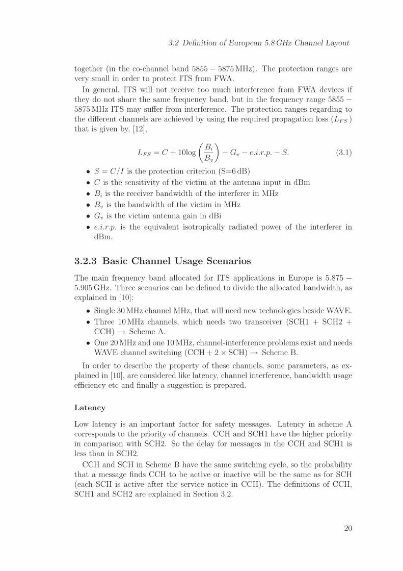
In general, ITS will not receive too much interference from FWA devices ifthey do not share the same frequency band, but in the frequency range 5855 −5875 MHz ITS may suffer from interference. The protection ranges regarding tothe different channels are achieved by using the required propagation loss (LFS )that is given by, [12],
LFS = C + 10log
(
Bi
Bv
)
− Gv − e.i.r.p. − S. (3.1)
• S = C/I is the protection criterion (S=6 dB)
• C is the sensitivity of the victim at the antenna input in dBm
• Bi is the receiver bandwidth of the interferer in MHz
• Bv is the bandwidth of the victim in MHz
• Gv is the victim antenna gain in dBi
• e.i.r.p. is the equivalent isotropically radiated power of the interferer indBm.
3.2.3 Basic Channel Usage Scenarios
The main frequency band allocated for ITS applications in Europe is 5.875 −5.905 GHz. Three scenarios can be defined to divide the allocated bandwidth, asexplained in [10]:
• Single 30 MHz channel MHz, that will need new technologies beside WAVE.
• Three 10 MHz channels, which needs two transceiver (SCH1 + SCH2 +CCH) → Scheme A.
• One 20 MHz and one 10 MHz, channel-interference problems exist and needsWAVE channel switching (CCH + 2 × SCH) → Scheme B.
In order to describe the property of these channels, some parameters, as ex-plained in [10], are considered like latency, channel interference, bandwidth usageefficiency etc and finally a suggestion is prepared.
Latency
Low latency is an important factor for safety messages. Latency in scheme Acorresponds to the priority of channels. CCH and SCH1 have the higher priorityin comparison with SCH2. So the delay for messages in the CCH and SCH1 isless than in SCH2.
CCH and SCH in Scheme B have the same switching cycle, so the probabilitythat a message finds CCH to be active or inactive will be the same as for SCH(each SCH is active after the service notice in CCH). The definitions of CCH,SCH1 and SCH2 are explained in Section 3.2.
20
3.2 Definition of European 5.8 GHz Channel Layout
Channel Interference
There is very limited interference in scheme A between CCH and SCH1, becausethese channels are non-adjacent. SCH2 has more interference with the otherchannels, but if SCH2 has lower power than CCH and SCH1 (for example 15 dBlower), then there will be no considerable interference from SCH2 on the other twochannels. Finally a problem remains, SCH2 always suffers by interference fromthe CCH and SCH1 (SCH2 has less priority in comparison with CCH and SCH1).
In scheme B if CCH be located between two SCHs, there will be no adjacentchannel interference, because each channel, CCH or SCH, works only on it’s owntime interval. But there exists still a small non-adjacent channel interference. Inthis situation, scheme B is slightly preferred.
Hardware
There are two channels in Scheme A that work at the same time, two wirelessnetwork interfaces are needed that may cause extra costs. In this case softwaredrivers are available for the hardware and so there will be no need to additionaldrivers. But Scheme B has one active channel at a time, so it needs only onewireless network interface, but requires an implementation of WAVE synchro-nized channel switching. Overall the Scheme B is slightly preferred over SchemeA, but it still depends on the hardware prices.
Bandwidth Usage Efficiency
In this section the efficiency of channel allocation is investigated according tothe duration of bandwidth usage. Bandwidth usage efficiency can be definedby E =
∑
Bandwidth × Percentage of active time. In scheme A, CCH andSCH1 can be active at the same time, so efficiency can be calculated easily by:EschemeA = 2 × 10 MHz × 100% = 10 MHz × 200%.
In scheme B, every channel can be active only half of the time, so the bandwidthusage efficiency is EschemeB = (1 × 20 MHz + 1 × 10 MHz) × (50% − x%) and xis the switching time. By comparing EschemeA and EschemeB, we can see thatScheme A is preferred over scheme B in this case.
Additional Frequency Band (5.905 - 5.925 GHz)
In scheme A the first lower 10 MHz channel of the additional bandwidth (5.905−5.925 GHz) can be like SCH2 with lower transmit power in compare with SCH1and CCH. The last channel can work similar to the SCH1. By this usage, thechannel usage efficiency will raise by 10MHz × 100%.
In Scheme B two 10 MHz channel can be added to the SCH. So the whole SCHbandwidth will be 40 MHz. But still the adjacent channel interference problem
21
3.2 Definition of European 5.8 GHz Channel Layout
exists with the new added channels, so both added channels can not work at thesame time. In this situation to reduce the adjacent channel interference, two newchannels can not work at the same time and so the active time should be reduced.Total channel usage efficiency increases by 10 MHz × 50% in scheme B, which isless than the increased efficiency in scheme A. Finally scheme A is preferred inthis case over scheme B.
Reliability
Reliability is also a critical factor for safety messages and therefore it is essentialfor the final suggestion. All devices must be synchronized in Scheme B, with aunit reference. Unsynchronized devices or any kind of inaccuracy can make theWAVE channel switching not possible. Scheme A has no need for synchronization.So scheme A is preferred over scheme B in the reliability evaluation.
Node Density and Prioritization
When the amount of nodes, that want to have communication together, increases,controlling the amount of data traffic will be important and it can be done bycontrolling the packet size, changing the packet generation rate and transmittingpower. Available congestion control mechanisms can be implemented on bothschemes, so there is no preference for these parameters. Also both schemes cancarry prioritization of different message types, so no preference will exist due tothis factor.
Briefly, the 30 MHz channel scenario requires new hardware (transceiver), whichis a drawback. Concurrent usage of two adjacent channels causes considerablepacket loss and also 20 MHz channels are more susceptible to BER than 10 MHzchannels. On the other hand interference happening between nonadjacent chan-nels is much lower than interference between the adjacent channels. Totally theadvantages of scheme A are greater than of scheme B. But Interference on neigh-boring systems and infects from other devices those investigated in sections 3.2.1and 3.2.2 can change this priority. These factors can be a good guide to decideon the extra bandwidth (5.905 − 5.925 GHz) usage. Using the extra band is anopen question and is still under investigation, [10].
22
Chapter 4
Measurements of TransmitterFrontend
In this chapter, measurements of different parameters are explained in detail andthe final results are compared with the specified values from IEEE 802.11p stan-dard. At the beginning, some test signals similar to the IEEE 802.11p signalsare generated by a Vector Signal Generator (VSG) from Rohde&Schwarz namedSMU -200A. There is a software related to this generator named WinIQSIMthat can generate IEEE 802.11a signals. The IEEE 802.11p test signals also couldbe generated after some changes. This software is connected to the SMU -200Athrough LAN and finally the desired test signal could be achieved in signal gen-erator’s output. After this measurements were done with a real IEEE 802.11pWLAN transceiver developed by Siemens AG Austria, introduced in Section 4.1in detail. Measurements were done at the transmitter like emission power, spec-tral emission, guard interval and ramp-up / ramp-down time. The measurementof some other parameters could not be implemented due to limited in access tothe physical layer parameters of the Device Under Test (DUT).
4.1 Siemens WLAN Transceiver (DUT)
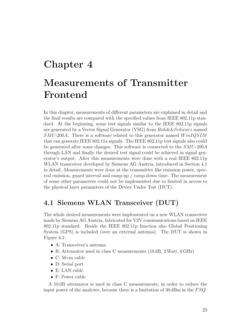
The whole desired measurements were implemented on a new WLAN transceivermade by Siemens AG Austria, fabricated for V2V communications based on IEEE802.11p standard. Beside the IEEE 802.11p function also Global PositioningSystem (GPS) is included (over an external antenna). The DUT is shown inFigure 4.1:
• A: Transceiver’s antenna
• B: Attenuator used in class C measurements (10 dB, 2 Watt, 6 GHz)
• C: 50 cm cable
• D: Serial port
• E: LAN cable
• F: Power cable
A 10 dB attenuator is used in class C measurements, in order to reduce theinput power of the analyzer, because there is a limitation of 30 dBm in the FSQ-
23
4.2 Measurement devices
A
A B CDEF
Figure 4.1: IEEE 802.11p Transceiver (Siemens).
26 spectrum analyzer (this analyzer is introduced in Section 4.2). In order towork in a linear area, it is suggested to work with an input power of 10 dBm atmaximum.
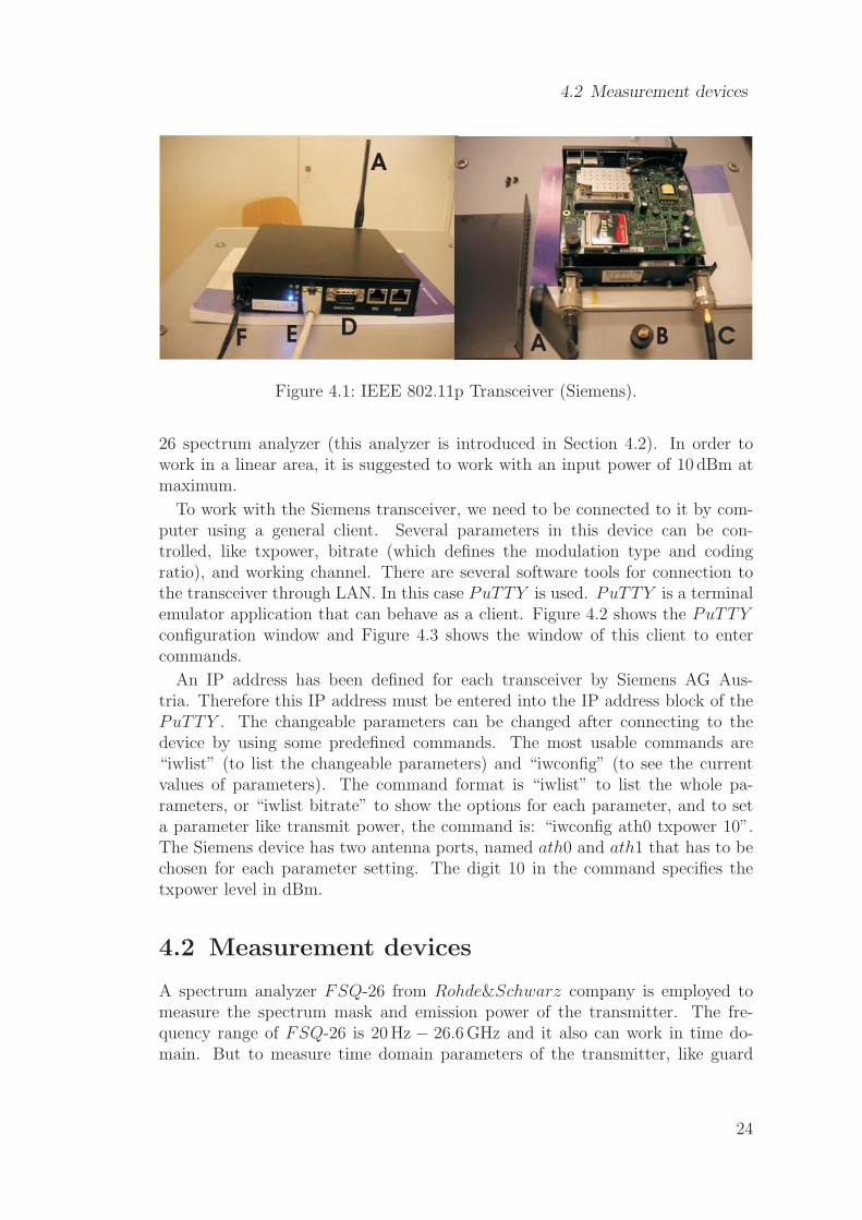
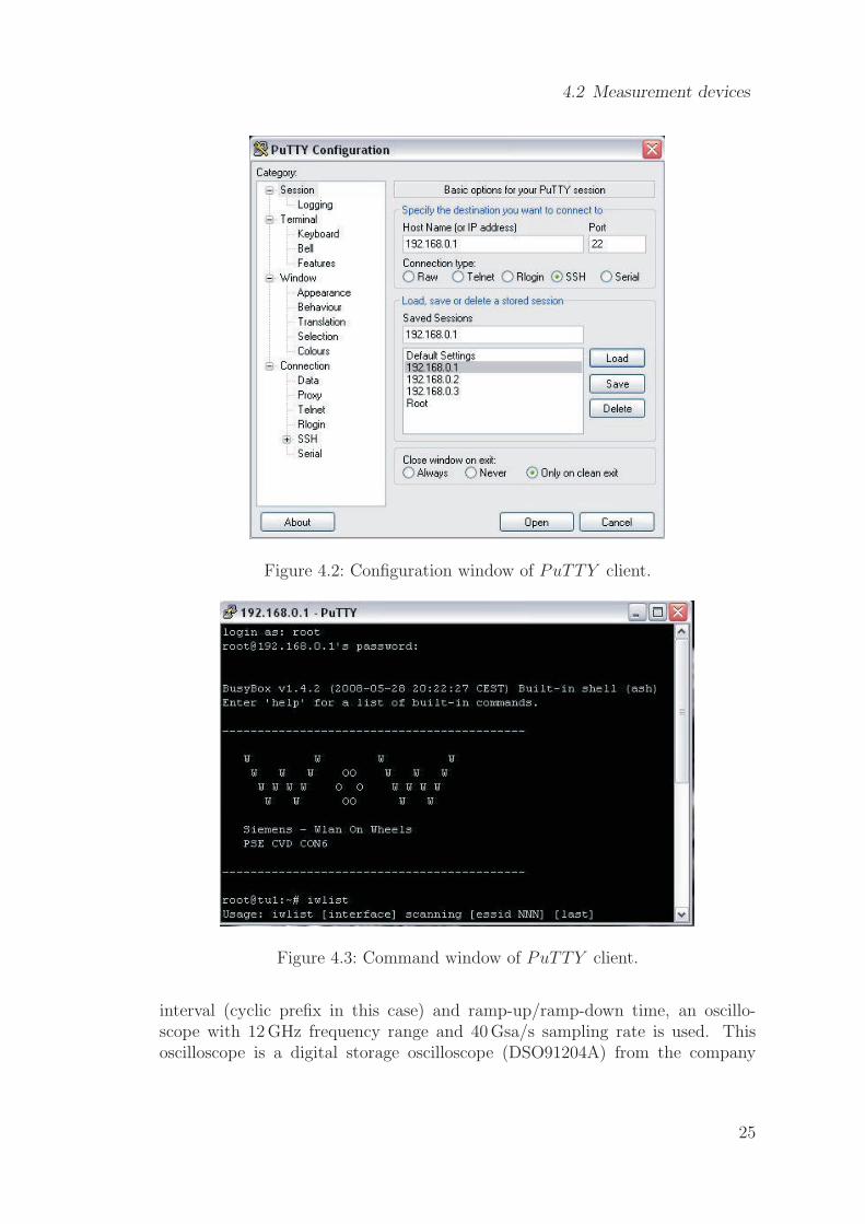
To work with the Siemens transceiver, we need to be connected to it by com-puter using a general client. Several parameters in this device can be con-trolled, like txpower, bitrate (which defines the modulation type and codingratio), and working channel. There are several software tools for connection tothe transceiver through LAN. In this case PuTTY is used. PuTTY is a terminalemulator application that can behave as a client. Figure 4.2 shows the PuTTYconfiguration window and Figure 4.3 shows the window of this client to entercommands.
An IP address has been defined for each transceiver by Siemens AG Aus-tria. Therefore this IP address must be entered into the IP address block of thePuTTY . The changeable parameters can be changed after connecting to thedevice by using some predefined commands. The most usable commands are“iwlist” (to list the changeable parameters) and “iwconfig” (to see the currentvalues of parameters). The command format is “iwlist” to list the whole pa-rameters, or “iwlist bitrate” to show the options for each parameter, and to seta parameter like transmit power, the command is: “iwconfig ath0 txpower 10”.The Siemens device has two antenna ports, named ath0 and ath1 that has to bechosen for each parameter setting. The digit 10 in the command specifies thetxpower level in dBm.
4.2 Measurement devices
A spectrum analyzer FSQ-26 from Rohde&Schwarz company is employed tomeasure the spectrum mask and emission power of the transmitter. The fre-quency range of FSQ-26 is 20 Hz − 26.6 GHz and it also can work in time do-main. But to measure time domain parameters of the transmitter, like guard
24
4.2 Measurement devices
Figure 4.2: Configuration window of PuTTY client.
Figure 4.3: Command window of PuTTY client.
interval (cyclic prefix in this case) and ramp-up/ramp-down time, an oscillo-scope with 12 GHz frequency range and 40 Gsa/s sampling rate is used. Thisoscilloscope is a digital storage oscilloscope (DSO91204A) from the company
25
4.3 Emission Power
Agilent Technologies. Figure 4.4 shows the employed oscilloscope connected tothe transceiver with a 50 cm coaxial cable.
Figure 4.4: Agilent Oscilloscope connected to the Siemens transceiver.
4.3 Emission Power
In this section, the setting of the transceiver and spectrum analyzer for emissionpower measuring is explained. Further the measurement results are comparedwith the specifications from IEEE 802.11p standard.
4.3.1 Measurement Set-Up
This test ensures that the maximum output power does not exceed the specifiedvalue. Excessive output power may result in blocking other WLAN devices fromtransmission or non-conformance with national regulations for the assigned fre-quency bands.
26
4.3 Emission Power
Present device (RouterBOARD 532A, Siemens) does not support class D, someasurements were done on class A, B and C (more details about transmissionclasses are explained in Section 2.2.1). To set the device to transmit in each class,we need to map the set value by software to the real output power. This meansthat Txpower of the DUT should be set on 6 dBm to be in the desired range ofclass A. According to the IEEE 802.11p standard it should be 0 dBm.
Emission power was measured with the signal analyzer (FSQ-26 Rohde&Schwarz).First of all, the centre frequency of the analyzer is set to the centre frequency ofworking channel. In this case channel number 184 (5.915 − 5.925 GHz) is used,so the frequency is set to 5.92 GHz. To see the whole signal of the channel andalso the shoulders of the signal (effect of the channel on the adjacent channels), a40 MHz span is defined. The signal reaches to the noise floor and has no effect onthe adjacent and non adjacent channels. The reference level of analyzer changesdepending on the transmission class. In this work, the reference level is set to20 dBm to cover the measurements in all classes.
The Resolution Bandwidth (RBW) specifies the FFT bin size and determinesthe smallest frequency that can be diagnosed and also determines the measure-ment precision. The higher RBW value the lower frequency resolution and viceversa. The smaller value of RBW is more efficient for narrow band signals due tohigher frequency resolution requirement. But in our case, the bandwidth of thechannel is 10 MHz, therefore 100 kHz RBW value can cover the required resolu-tion.
To see a more reliable signal, the RMS detector is selected to display the RMSvalue of measured power. Therefore the root mean square of all sampled levelvalues is formed during the sweep of a pixel. The sweep time determines thenumber of averaged values and with increasing sweep time a better averagingresult can be obtained. The video bandwidth must be at least 10 times of theselected RBW (in our case: 10× 100 kHz = 1 MHz) to ensure that video filteringdoes not cancel the RMS values of the signal. The display for small signals is,however, the sum of signal power and noise power. For short sweep times, theRMS detector is equivalent to the sample detector. If the sweep time is longer,more and more uncorrelated RMS values supply the RMS value measurementand therefore the trace becomes more smooth. At a RBW of 100 kHz the maxi-mum frequency display range is 62.5 MHz (suitable for our case) and higher sweeptime causes smoother and more stable signal. The best choice for sweep time isthe smallest possible value for a given span and resolution bandwidth. Overallthe sweep time is selected to 200 ms according to the 40 MHz span and 100 kHzRBW, [13].
After choosing the setting, the channel power measurement configuration isenabled and then 10 MHz is defined for the channel bandwidth. The signal ana-
27
4.3 Emission Power
lyzer’s setting is as following:
• Frequency: 5.92 GHz, Centre frequency of working channel (channel 184)
• Span: 40 MHz to see the complete signal
• Reference level: Maximum expected output power, depends on workingclass, (I set this parameter on 20 dBm to cover all classes)
• RBW: 100 kHz
• VBW: 1 MHz
• Sweep time: 200 ms
• Detector: RMS detector sweep
• Channel power ACP → CP / ACP Config → Channel bandwidth: 10 MHz(ACP is pointing to adjacent channel power and CP is pointing to channelpower)
4.3.2 Measurement Results
For Class A, maximum specified Txpower is equal to 0 dBm. Figure 4.5 showsthe analyzer screen shot for this measurement. The measured value for class Ais 1.8 dBm that is slightly higher than standard definition. In this class, trans-mitter is set by software to 6 dBm, which means that there is an offset betweenthe software set power and the read output power.
Figure 4.5: Measurement result for emission power in class A.
For Class B, maximum specified Txpower is equal to 10 dBm. Figure 4.6 showsthat the emission power in class B is 9.24 dBm and therefore this value is locatedin the predefined range from the standard.
28
4.3 Emission Power
Figure 4.6: Measurement result for emission power in class B.
For Class C, maximum specified Txpower is equal to 18 dBm. As illustratedin Figure 4.7, emission power is equal to 17.66 dBm, therefore transmitter worksproperly in this class.
Figure 4.7: Measurement result for emission power in class C.
These measurement were done in channel 184 (5.915 − 5.925 GHz). Investi-gation of the measurement in other channels of IEEE 802.11p shows the sameresults for the DUT (RouterBOARD 532A, Siemens).
Consideration of total emission power shows that the device can be used in classB and C without any problem, in class A the output power is slightly higher thanthe maximum allowed output power.
29
4.4 Spectral Emission
4.4 Spectral Emission
Emission power spectrum mask measurement are done to ensure that the DUTdoes not manipulate WLAN devices working in adjacent channels. Transmitterfilter is not defined in IEEE 802.11p standard, but transmitter spectrum mask isdefined and must be passed. Therefore, design of the transmitter shall fulfill thespecification of spectrum mask defined by IEEE 802.11p standard, [14].
To see the spectrum mask of the transmitter working with OFDM signals,there is an option that can be installed on the signal analyzer FSQ − 26. Thisoption is named WLAN and designed for working under IEEE 802.11a, b, g, jstandards. The other way is a manual setting of the analyzer for such a signal.In this case, I set the analyzer manually step by step.
There are 4 classes of transmitters defined in IEEE 802.11p and each case hasits own mask. The mask regarding to the class A, B, C, D are shown in Figure4.8.
A B
C D
Figure 4.8: Class A, B, C, and D spectrum masks defined in IEEE 802.11p stan-dard.
4.4.1 Measurement Set-Up
First of all, each mask is defined manually for the analyzer. For this purpose,the ”Lines” menu is used. Limit lines are defined for the analyzer to determinespectral distribution boundaries. These lines point to the upper limits for radia-tion to prevent interfering to other systems and also to protect the human from
30
4.4 Spectral Emission
high power radiations.
For each limit line regarding to each transmission class, the following charac-teristics are defined in frequency domain:
1. The name of the limit line.
2. The reference of the interpolation points to the X axis.
3. The reference of the interpolation points to the Y axis.
4. The limit line units to be used. The units of the limit line must be com-patible with the level axis in the measurement window.
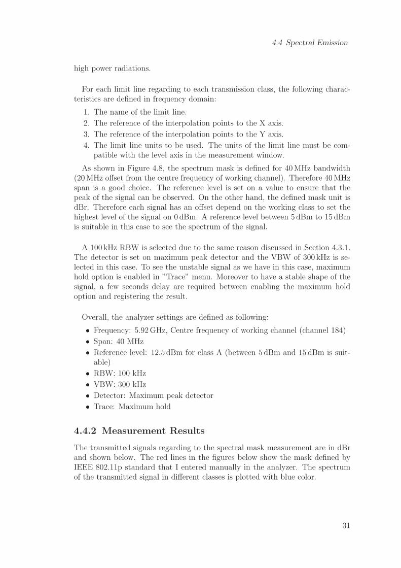
As shown in Figure 4.8, the spectrum mask is defined for 40 MHz bandwidth(20 MHz offset from the centre frequency of working channel). Therefore 40 MHzspan is a good choice. The reference level is set on a value to ensure that thepeak of the signal can be observed. On the other hand, the defined mask unit isdBr. Therefore each signal has an offset depend on the working class to set thehighest level of the signal on 0 dBm. A reference level between 5 dBm to 15 dBmis suitable in this case to see the spectrum of the signal.
A 100 kHz RBW is selected due to the same reason discussed in Section 4.3.1.The detector is set on maximum peak detector and the VBW of 300 kHz is se-lected in this case. To see the unstable signal as we have in this case, maximumhold option is enabled in ”Trace” menu. Moreover to have a stable shape of thesignal, a few seconds delay are required between enabling the maximum holdoption and registering the result.
Overall, the analyzer settings are defined as following:
• Frequency: 5.92 GHz, Centre frequency of working channel (channel 184)
• Span: 40 MHz
• Reference level: 12.5 dBm for class A (between 5 dBm and 15 dBm is suit-able)
• RBW: 100 kHz
• VBW: 300 kHz
• Detector: Maximum peak detector
• Trace: Maximum hold
4.4.2 Measurement Results
The transmitted signals regarding to the spectral mask measurement are in dBrand shown below. The red lines in the figures below show the mask defined byIEEE 802.11p standard that I entered manually in the analyzer. The spectrumof the transmitted signal in different classes is plotted with blue color.
31
4.4 Spectral Emission
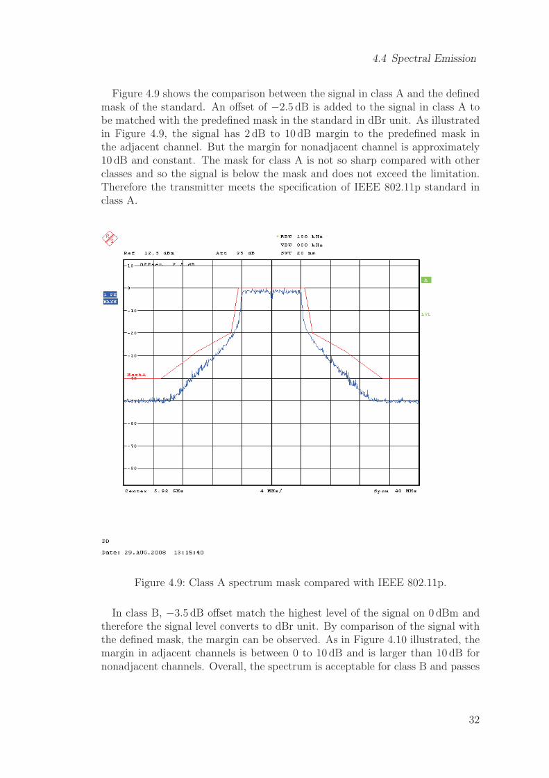
Figure 4.9 shows the comparison between the signal in class A and the definedmask of the standard. An offset of −2.5 dB is added to the signal in class A tobe matched with the predefined mask in the standard in dBr unit. As illustratedin Figure 4.9, the signal has 2 dB to 10 dB margin to the predefined mask inthe adjacent channel. But the margin for nonadjacent channel is approximately10 dB and constant. The mask for class A is not so sharp compared with otherclasses and so the signal is below the mask and does not exceed the limitation.Therefore the transmitter meets the specification of IEEE 802.11p standard inclass A.
Figure 4.9: Class A spectrum mask compared with IEEE 802.11p.
In class B, −3.5 dB offset match the highest level of the signal on 0 dBm andtherefore the signal level converts to dBr unit. By comparison of the signal withthe defined mask, the margin can be observed. As in Figure 4.10 illustrated, themargin in adjacent channels is between 0 to 10 dB and is larger than 10 dB fornonadjacent channels. Overall, the spectrum is acceptable for class B and passes
32
4.5 Error Vector Magnitude
the necessary specifications.
Figure 4.10: Class B spectrum mask compared with IEEE 802.11p.
Comparison of class C with related mask shows that the spectrum of trans-mitted signal can not follow the defined mask and exceeds in both, adjacentchannels and nonadjacent channels. One point should be mentioned that theedges of the spectrum mask defined by IEEE 802.11p standard are sharper inthis class compared with class A and B. Figure 4.11 illustrates the predefinedmask and transmitted spectrum from the DUT (RouterBOARD 532A, Siemens).
4.5 Error Vector Magnitude
To measure the Error Vector Magnitude (EVM), a Vector Signal Analyzer (VSA)(for example FSQ-K70 Rohde&Schwarz) can be used. There are several possi-bilities to measure the EVM from an OFDM signal:
33
4.5 Error Vector Magnitude
Figure 4.11: Class C spectrum mask compared with IEEE 802.11p.
• MATLAB: Importing the signal to MATLAB, demodulation and calculat-ing the EVM by signal processing. It takes a lot of work and time.
• Carrier: In this case the EVM could be measured individually for each car-rier. One subcarrier can be selected and be sent to the VSA as a single car-rier signal to measure the EVM. For this purpose, the transmitted signal’sspecifications must be known and also we must have access to the subcarri-ers for edition (at present DUT, ”RouterBOARD 532A” transceiver, thereis no access to the subcarriers). Following parameters must be defined atthe VSA before EVM measurement.
– Modulation type
– Bitrates
– Modulation filter type
Possible choices for these parameters can be found in Table 3.1.
• Using an OFDM demodulator software based on IEEE 802.11p in the VSA:The software option K96 is a general OFDM demodulator and not specified
34
4.6 Guard Intervals
for IEEE 802.11p signals. There are some other options specialized for IEEE802.11a,b,g but still nothing designed for IEEE 802.11p.
Due to limitation in time and available equipment during the thesis workingperiod, it was not possible to measure the EVM.
4.6 Guard Intervals
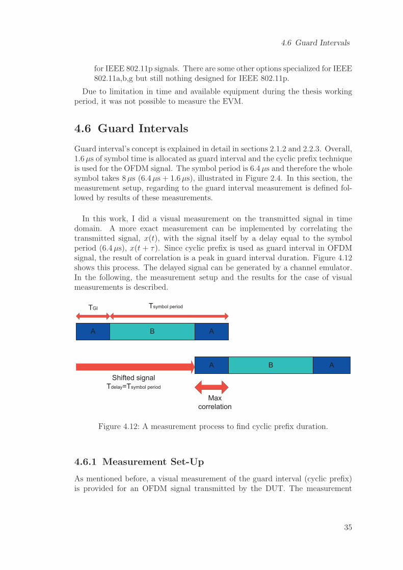
Guard interval’s concept is explained in detail in sections 2.1.2 and 2.2.3. Overall,1.6 µs of symbol time is allocated as guard interval and the cyclic prefix techniqueis used for the OFDM signal. The symbol period is 6.4 µs and therefore the wholesymbol takes 8µs (6.4 µs + 1.6 µs), illustrated in Figure 2.4. In this section, themeasurement setup, regarding to the guard interval measurement is defined fol-lowed by results of these measurements.
In this work, I did a visual measurement on the transmitted signal in timedomain. A more exact measurement can be implemented by correlating thetransmitted signal, x(t), with the signal itself by a delay equal to the symbolperiod (6.4 µs), x(t + τ). Since cyclic prefix is used as guard interval in OFDMsignal, the result of correlation is a peak in guard interval duration. Figure 4.12shows this process. The delayed signal can be generated by a channel emulator.In the following, the measurement setup and the results for the case of visualmeasurements is described.
A
A
B A
B A
TGI Tsymbol period
Shifted signal
Tdelay=Tsymbol period
Max
correlation
Figure 4.12: A measurement process to find cyclic prefix duration.
4.6.1 Measurement Set-Up
As mentioned before, a visual measurement of the guard interval (cyclic prefix)is provided for an OFDM signal transmitted by the DUT. The measurement
35
4.6 Guard Intervals
is done in time domain, implemented with the oscilloscope introduced in section4.2. The transmitter is set to transmit signal in class B (10 dBm emission power),with 9 Mb/s data rate and centre frequency of 5.92 GHz (channel number 184).At the oscilloscope the vertical scale is set to 1 V and horizontal scale is set to1 µs, therefore 10 µs of the signal can be observed on the screen (the length of asymbol is 8 µs).
4.6.2 Measurement Results
The transmitted data is a periodic random signal. We know that the cyclic prefixtechnique is used in the transmitted signal. This means if we find two parts inthe signal with 1.6 µs length, similar to each other, we can say that one of themis cyclic prefix and the other one is the last part of the symbol that is repeatedat the beginning. Figure 4.13 shows 10µs of the transmitted signal. T is thewhole symbol duration plus the cyclic prefix, equal to 8µs and the Tsymb is thesymbol duration, equal to 6.4 µs (8 µs − 1.6 µs). The left red arrow shows thecyclic prefix of the signal with duration of approximately 1.6 µs, that meets thespecifications of the IEEE 802.11p standard.
TGI
Tsymb
T
Figure 4.13: Cyclic prefix visualizing.
36
4.7 Ramp-Up/Ramp-Down Time
4.7 Ramp-Up/Ramp-Down Time
Ramp-up and ramp-down duration show the rapidity of the device reaching toa stable carrier level depending on transmitter’s working class. Different trans-mitter classes are explained in section 2.2.1 in detail. Data transferring in anOFDM signal shall be started with a delay larger than the ramp-up duration.IEEE 802.11 standard defines a maximum 2µs for ramp-up/down duration forDirect Sequence Spread Spectrum (DSSS) signal, [4], and there is no specifieddefinition for ramp-up/down time for OFDM signals in IEEE 802.11p standard.Therefor I assumed this limitation value be the same for IEEE 802.11p, too. Re-sults of measurements can be optimized by finding the stable level of the carrierswith higher accuracy (Max Hold detection in oscilloscope). But I do not expectconsiderable differences. In the case of using the Max Hold, it is necessary to setthe trigger to see a stable signal on the screen.
4.7.1 Measurement Set-Up
To measure the ramp-up / ramp-down duration for class B and C, the verticaland horizontal scale of the oscilloscope is set on 1 V and 5µs, respectively. By thissetting the first part of the signal can be observed, which shows the transmissionstart time and data sending time. In class A, the vertical scale is set to 500 mVdue to lower emission power. Then the horizontal scale is reduced to find thestable level of the carrier before data transmission. After calculation of 10 %and 90 % of the stable level, and locating the horizontal markers on these levels,the vertical markers location can be find to measure the ramp-up duration. Theleft marker is placed on the junction of lower horizontal marker with the signal,and the right marker shows the first point where the signal reaches the upperhorizontal level. The transceiver is transmitting 9 Mbit/s data rate and is workingin channel 184. The next section shows to the results of ramp-up measurements.First of all, the transceiver is set to class C and a 10 dB attenuator is used toprotect the oscilloscope (4 V is the limitation of input voltage in the oscilloscope).
4.7.2 Measurement Result
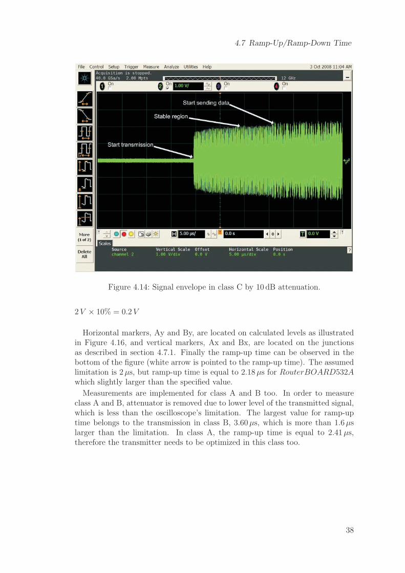
Figure 4.14 shows the start point of transmission of a packet of data (each packettakes 4 ms). Carriers are reaching to the stable level after approximately 10µs,and then data transmission is started by 16µs delay from start transmissionpoint.
The next task is to find the stable level of the carriers, illustrated in Figure4.15. The maximum stable level is approximately at 2 V and a marker Ay islocated on this point. Now 10 % and 90 % of this level are calculated accordingto the ramp-up definition:2 V × 90% = 1.8 V
37
4.7 Ramp-Up/Ramp-Down Time
Figure 4.14: Signal envelope in class C by 10 dB attenuation.
2 V × 10% = 0.2 V
Horizontal markers, Ay and By, are located on calculated levels as illustratedin Figure 4.16, and vertical markers, Ax and Bx, are located on the junctionsas described in section 4.7.1. Finally the ramp-up time can be observed in thebottom of the figure (white arrow is pointed to the ramp-up time). The assumedlimitation is 2µs, but ramp-up time is equal to 2.18 µs for RouterBOARD532Awhich slightly larger than the specified value.
Measurements are implemented for class A and B too. In order to measureclass A and B, attenuator is removed due to lower level of the transmitted signal,which is less than the oscilloscope’s limitation. The largest value for ramp-uptime belongs to the transmission in class B, 3.60 µs, which is more than 1.6 µslarger than the limitation. In class A, the ramp-up time is equal to 2.41 µs,therefore the transmitter needs to be optimized in this class too.
38
4.7 Ramp-Up/Ramp-Down Time
Figure 4.15: Stable level of carriers in class C by 10 dB attenuation.
Figure 4.16: Ramp-up observation in class C by 10 dB attenuation.
39
Chapter 5
Summary
In this thesis, I first described fundamentals of OFDM transmission and frontendcharacterization parameters in general. I further extended these investigation tothe specifications of IEEE 802.11p standard regarding to each parameter. Thisdefines the expected requirements of an inter-vehicle communication transceiver.
Then specifications of a WLAN transmission based on IEEE 802.11p are stud-ied and different possibilities of the bandwidth usage are evaluated.
The RF frontend consists of transmitter, receiver and local oscillators. Themain work of this thesis was performing different measurements to evaluate theperformance of the transmitter. After research on expected values for each pa-rameter, the measurement setup was implemented and the results were comparedwith IEEE 802.11p standard specifications. The measurement setup and resultshave been given in Chapter 4. The results describe the behavior of the transmit-ter in the frequency domain as well as in the time domain and at different powerlevels. Furthermore they show how much the transmitter fulfills its specifications.
In the case of measuring the emission power, the results for transmission classesB and C are fulfilled, but the transmitter needs some optimization in class A.The spectrum of the emission signal meets the specifications in classes A andB, but the spectrum in class C exceeds the limitations. The guard interval ofthe transmitted signal meets the specifications of the standard. Also ramp-downtime fulfilled the requirements. In the case of ramp-up measurement the mea-sured times are slightly more than the expected values in all classes.
Overall, the work on other parts of RF frontend like receiver and the localoscillator, measuring of the other frontend parameters like EVM and IP3, andthe ability of receiver to mitigate the effect of fading in data transmission arenecessary to have a reliable evaluation on the DUT.
40
Bibliography
[1] C. D. Wang and J. P. Thompson, “Apparatus and method for motion detec-tion and tracking of objects in a region for collision avoidance utilizing a real-time adaptive probabilistic neural network,” in US. Patent No. 5,613,039,1997.
[2] X. Yang, J. Liu, F. Zhao, and N. H. Vaidya, “A vehicle-to-vehicle com-munication protocol for cooperative collision warning,” in 1st InternationalConference on Mobile and Ubiquitous Systems: Networking and Services(Mobiquitous 2004), Boston, MA, 22-26 August 2004.
[3] “Part 11: Wireless LAN medium access control (MAC) and physical layer(PHY) specifications amendment 8: Wireless access in vehicular environ-ments,” IEEE P802.11ptm /D4.0, March 2008.
[4] “Part 11: Wireless LAN medium access control (MAC) and physical layer(PHY) specifications,” ANSI/IEEE Std. 802.11, 1999 (R2003).
[5] http://zone.ni.com/devzone/cda/tut/p/id/3740, national Instruments.
[6] T. S. Rappaport, Wireless Communications: Principles and Practice, 2ndedition. Prentice-Hall, Inc., 2001.
[7] Y. Zang, L. Stibor, G. Orfanos, S. Guo, and H. J. Reuerman, “An errormodel for inter-vehicle communications in highway scenarios at 5.9GHz,” inInternational Workshop on Modeling Analysis and Simulation of Wirelessand Mobile Systems, 2005.
[8] http://www.its.bldrdoc.gov, institute for Telecommunication Sciences.
[9] “Part 11: Wireless LAN medium access control (MAC) and physical layer(PHY) specifications, high-speed physical layer in the 5 GHz band,” IEEEStd. 802.11a, 1999 (R2003).
[10] L. Le, W. Zhang, A. Festag, and R. Baldessari, “Analysis of approachesfor channel allocation in car-to-car communication,” in First internationalconference on the internet of things (IOT 2008) Workshop, 2008.
[11] “Electromagnetic compatibility and radio spectrum matters (ERM); intel-ligent transport systems (ITS), technical report, draft ETSI TR 102 492-2,V1.1.1 0.0.16,” ETSI Technical Committee Electromagnetic compatibilityand Radio spectrum Matters (ERM), Tech. Rep., 2006.
[12] “Compatibility studies in the band 5855 5925 MHz between intelligent trans-port system (ITS) and other systems,” Electronic Communications Commit-tee, ECC report 101, Tech. Rep., 2007.


![Imam Mahdi [AS]](https://static.documents.pub/doc/80x56/546492ecaf79596e458b462f/imam-mahdi-as.jpg)


