GHENT UNIVERSITY FACULTY OF PHARMACEUTICAL SCIENCES Department of Bio Analysis Laboratory of Food Analysis Master thesis performed at: NATIONAL INSTITUTE OF OCCUPATIONAL HEALTH Department of the Chemical and Biological Work Environment Academic year 2014-2015 UNTARGETED METABOLOMICS IN OCCUPATIONAL HEALTH – THE SEWAGE WORKER CASE Florence GOETHALS First Master of Pharmaceutical Care Promoter: Prof. Dr. Apr. S. De Saeger co-promoter: Dr. S. Uhlig Commissioners: Dr. M. De Boevre Prof. Dr. K. Audenaert
Transcript
GHENT UNIVERSITY
FACULTY OF PHARMACEUTICAL SCIENCES
Department of Bio Analysis
Laboratory of Food Analysis
Master thesis performed at:
NATIONAL INSTITUTE OF OCCUPATIONAL
HEALTH
Department of the Chemical and
Biological Work Environment
Academic year 2014-2015
UNTARGETED METABOLOMICS IN OCCUPATIONAL HEALTH – THE SEWAGE WORKER CASE
Florence GOETHALS
First Master of Pharmaceutical Care
Promoter:
Prof. Dr. Apr. S. De Saeger
co-promoter:
Dr. S. Uhlig
Commissioners:
Dr. M. De Boevre
Prof. Dr. K. Audenaert
GHENT UNIVERSITY
FACULTY OF PHARMACEUTICAL SCIENCES
Department of Bio Analysis
Laboratory of Food Analysis
Master thesis performed at:
NATIONAL INSTITUTE OF OCCUPATIONAL
HEALTH
Department of the Chemical and
Biological Work Environment
Academic year 2014-2015
UNTARGETED METABOLOMICS IN OCCUPATIONAL HEALTH – THE SEWAGE WORKER CASE
Florence GOETHALS
First Master of Pharmaceutical Care
Promoter:
Prof. Dr. Apr. S. De Saeger
Co-promoter:
Dr. S. Uhlig
Commissioners:
Dr. M. De Boevre
Prof. Dr. K. Audenaert
COPYRIGHT
“The author and the promoters give the authorization to consult and to copy parts of this
thesis for personal use only. Any other use is limited by the laws of copyright, especially
concerning the obligation to refer to the source whenever results from this thesis are cited.”
May …, 2015
Promoter Author
Prof. Dr. S. De Saeger Florence Goethals
SUMMARY
Due to the increasing doubt about the safety among sewage workers in occupational
health, there is a need to gain better insight into these workers’ state of health. Previous
investigations already found out that these individuals suffer from headache, lung function
reduction, irritation of the respiratory tract etc. due to daily exposure to potential harmful
contaminants in sewage. With the major objective to investigate these workers’ health more
thoroughly, differences between exposed individuals and others, who work in safe and
healthy environments, had to be established. Therefore, an untargeted HPLC-HRMS
metabolomics approach using serum samples was chosen in order to discover metabolic
changes in sewage workers as a result of the exposures in their working environment.
Serum samples were analyzed by two orthogonal HPLC-HRMS methods employing
either hydrophilic interaction liquid chromatography or reversed-phase HPLC. Raw data
were preprocessed using MZmine in order to create data sets consisting of “true” metabolic
features. Comparison of the two groups (i.e. exposed vs. control), was then performed using
multivariate data analyses included principal component analysis (PCA) and orthogonal
partial least squares – discriminant analysis (OPLS-DA). Extraction of the most significant
variables from the OPLS-DA models resulted finally in 13 potential metabolic markers out of
1000’s. The identity for eight of these could tentatively be established based on calculation
of elemental formulae, database searches and study of MS2 product ion spectra obtained
from data-depending scanning using ion trap MS. The tentatively identified metabolites
were two amino acids (phenylalanine, tyrosine) a dipeptide (phe-phe) and phosphocholines.
Whether or not these metabolites can be used for further elucidation of the adverse effects
connected to working in a sewage environment needs to be shown in the future.
SAMENVATTING
Door de toenemende onzekerheid omtrent de veiligheid van arbeiders in riool- en
afvalwaterzuiveringsfabrieken is er nood aan betere inzichten betreffende de
gezondheidstoestand van deze arbeiders. Eerder onderzoek heeft reeds aangetoond dat
deze individuen gevoelig kunnen zijn aan hoofdpijn, daling in longfunctie, luchtwegirritatie
etc. als gevolg van dagelijkse blootstelling aan potentieel schadelijke verontreinigingen in
afval- en rioolwater. Met als hoofddoelstelling om de gezondheid van deze arbeiders meer
diepgaand te onderzoeken, diende een vergelijking tussen deze blootgestelde individuen en
andere, werknemers in veilige en gezonde werkomstandigheden, gemaakt te worden.
Hiervoor wordt gebruik gemaakt van een untargeted HPLC-HRMS metabolomics methode,
met de bedoeling om metabolische veranderingen te detecteren in het metaboloom van
deze arbeiders als gevolg van blootstelling in hun werkomgeving.
Analyse van serum stalen werd uitgevoerd met behulp van twee orthogonale HPLC-
HRMS methoden, enerzijds hydrofilic interaction liquid chromatography en anderzijds
reversed-phase HPLC. Met behulp van MZmine werd de onbewerkte data behandeld, met
de bedoeling om data sets te ontwikkelen waarin informatie over de optimaal bruikbare
metabolieten aanwezig is. Vergelijking tussen de twee groepen (i.e. blootgesteld vs.
controle) was vervolgens mogelijk door gebruik te maken van multivariate data analyse,
betreffende principal component analysis (PCA) en orthogonal partial least squares –
discriminant analysis (OPLS-DA). Extractie van de meest significante variabelen van de OPLS-
DA modellen resulteerde uiteindelijk in 13 potentiele metabolomische biomarkers uitgaande
van meer dan duizenden metabolieten. De identiteit van acht van deze metabolieten kon
onder voorbehoud vastgesteld worden, gebaseerd op het bepalen van de elementaire
compositie, database zoekopdrachten en het bestuderen van de MS2 ion spectra. De
voorlopig geïdentificeerde metabolieten waren twee aminozuren (phenylalanine, tyrosine)
een dipeptide (phenylalanine-phenylalanine) en fosfocholines. Of deze metabolieten al dan
niet kunnen gebruikt worden voor verdere verduidelijking van de schadelijke effecten die
verbonden zijn aan de risicovolle werkomgeving, dient aangetoond te worden in de
toekomst.
THANKS TO
First of all, I would like to thank Prof. Dr. S. De Saeger for giving me the opportunity to work
and write on my thesis abroad. In particular I would like to thank Dr. S. Uhlig for the excellent
guidance concerning all the work, for everything I learned during the past few months and
most of all that he would take a lot of time for correcting and giving feedback on my thesis.
Apart from this, I would like to thank everybody at STAMI, for being warm-hearted and
helpful and especially, for all the experience I gained during work. Besides this, I also like to
thank all the people I met during my stay in Norway, for all the experiences and the beautiful
memories. I want to thank my family for giving me the possibility and the faith in me to study
abroad. At last I want to thank my boyfriend for the visits and his support.
3.4.2.3 Peak list alignment ................................................................................................................. 20
3.4.2.4 Gap filling ................................................................................................................................ 21
3.4.2.5 Peak list filtering ..................................................................................................................... 22
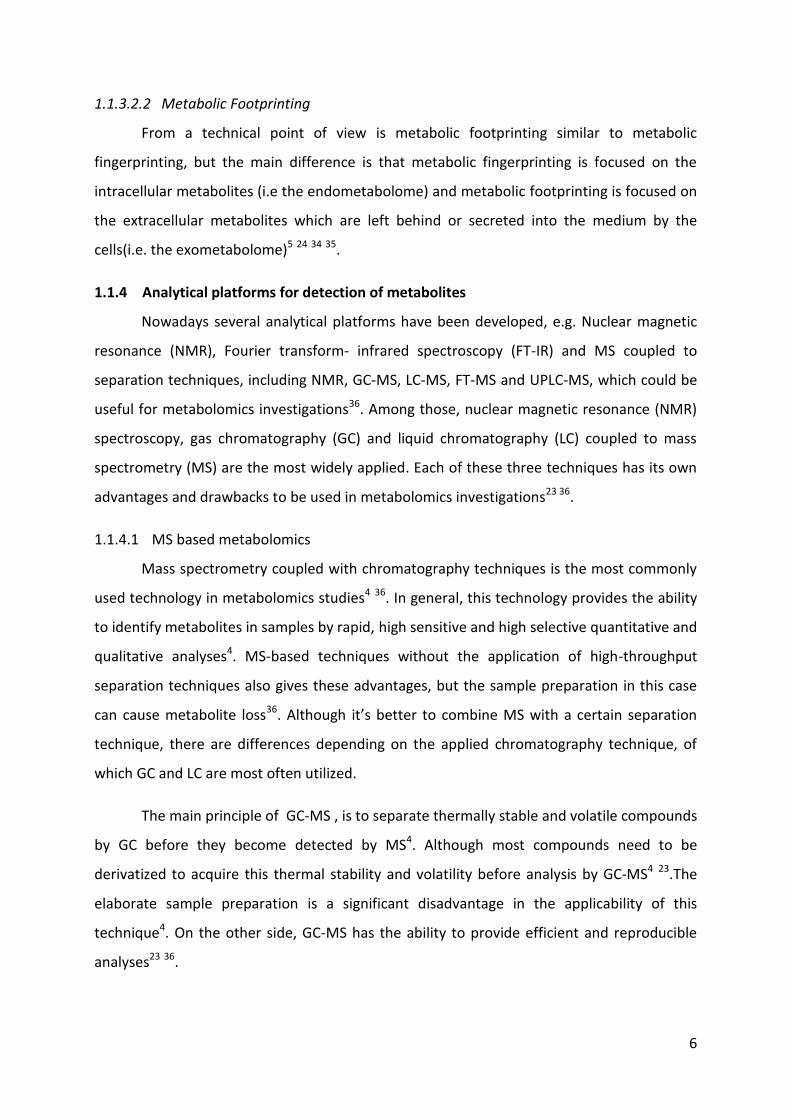
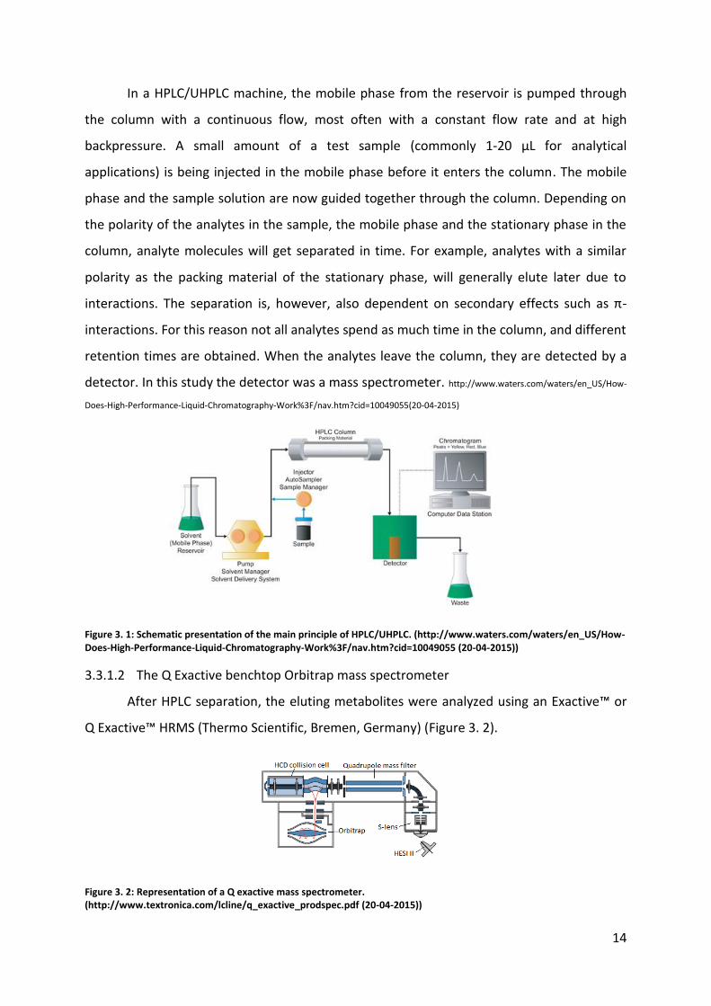
Figure 3. 1: Schematic presentation of the main principle of HPLC/UHPLC. (http://www.waters.com/waters/en_US/How-Does-High-Performance-Liquid-Chromatography-Work%3F/nav.htm?cid=10049055 (20-04-2015))
3.3.1.2 The Q Exactive benchtop Orbitrap mass spectrometer
After HPLC separation, the eluting metabolites were analyzed using an Exactive™ or
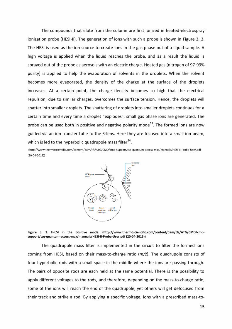
Figure 3. 3: H-ESI in the positive mode. (http://www.thermoscientific.com/content/dam/tfs/ATG/CMD/cmd-support/tsq-quantum-access-max/manuals/HESI-II-Probe-User.pdf (20-04-2015))
The quadrupole mass filter is implemented in the circuit to filter the formed ions
coming from HESI, based on their mass-to-charge ratio (m/z). The quadrupole consists of
four hyperbolic rods with a small space in the middle where the ions are passing through.
The pairs of opposite rods are each held at the same potential. There is the possibility to
apply different voltages to the rods, and therefore, depending on the mass-to-charge ratio,
some of the ions will reach the end of the quadrupole, yet others will get defocused from
their track and strike a rod. By applying a specific voltage, ions with a prescribed mass-to-
16
charge ratio will get focused, while the others get eliminated. Additionally it’s also possible
to employ alterations in the voltage, so ions with a certain range of mass-to-charge ratios
can be filtered55.
For a full scan analysis, the ions are accumulated in the C-trap after they went
through the quadrupole and are now led to the orbitrap, while clustering into a small ion
cloud. In the orbitrap, the ions circulate in an orbital motion between a central and a coaxial
electrode. This motion creates an image current that is detected, and the chromatograms
are built after Fourier-transformation of the measured current. In order to perform MS
fragmentation experiments, selected ions may be transferred to a higher-collision
dissociation (HCD) cell where fragmentation occurs, before the product ions are analyzed in
the orbitrap55 56.
3.3.2 RP-HPLC
Two different RP-HPLC columns have been used in this study. In previous analyses,
performed at the University of Strathclyde, an ACE Excel3 Super C18 column was used
(Advanced Chromatography Technologies Ltd., Aberdeen, Scotland; 150 × 3.0 mm i.d.). For
RP-HPLC-HRMS analyses in Oslo, the column of choice was a Kinetex™ XB-C18 column
(Phenomenex, Torrance, CA, USA; 100 × 2.1 mm i.d., 1.7 µm particle size). Both stationary
phases had a pore size of 100 Å.
The mobile phase consisted of 0.1% formic acid in purified water (mobile phase A)
and acetonitrile (mobile phase B)23 57.
A 5-µL aliquot of each sample was injected, and the column was kept at 30°C during
the entire run. The column was eluted using a linear gradient as shown in Table 3. 2.
Table 3. 2: The multi-step gradient for the RP-HPLC analysis using the Kinetex XB-C18 column.
Minimum ratio of peak top/edge 5 Peak duration range (min) 0.2-5
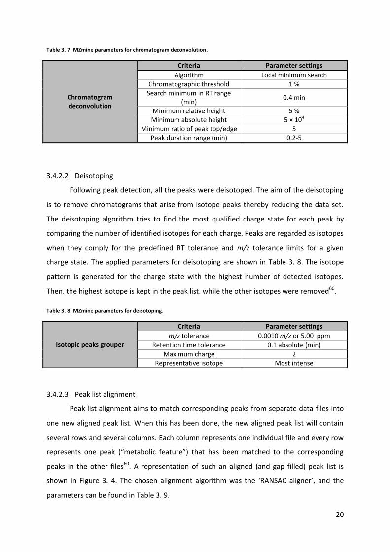
3.4.2.2 Deisotoping
Following peak detection, all the peaks were deisotoped. The aim of the deisotoping
is to remove chromatograms that arise from isotope peaks thereby reducing the data set.
The deisotoping algorithm tries to find the most qualified charge state for each peak by
comparing the number of identified isotopes for each charge. Peaks are regarded as isotopes
when they comply for the predefined RT tolerance and m/z tolerance limits for a given
charge state. The applied parameters for deisotoping are shown in Table 3. 8. The isotope
pattern is generated for the charge state with the highest number of detected isotopes.
Then, the highest isotope is kept in the peak list, while the other isotopes were removed60.
Table 3. 8: MZmine parameters for deisotoping.
Isotopic peaks grouper
Criteria Parameter settings
m/z tolerance 0.0010 m/z or 5.00 ppm Retention time tolerance 0.1 absolute (min)
Maximum charge 2 Representative isotope Most intense
3.4.2.3 Peak list alignment
Peak list alignment aims to match corresponding peaks from separate data files into
one new aligned peak list. When this has been done, the new aligned peak list will contain
several rows and several columns. Each column represents one individual file and every row
represents one peak (“metabolic feature”) that has been matched to the corresponding
peaks in the other files60. A representation of such an aligned (and gap filled) peak list is
shown in Figure 3. 4. The chosen alignment algorithm was the ‘RANSAC aligner’, and the
parameters can be found in Table 3. 9.
21
Table 3. 9: MZmine parameters for peak list alignment.
Peak list alignment
Criteria Parameter settings
Algorithm RANSAC aligner m/z tolerance 0.001 m/z or 5ppm
Retention time tolerance after correction
0.8 min
Retention time tolerance 0.8 min RANSAC iterations 15 000
Minimum number of points 20.00 % Threshold value 2
Linear model No
3.4.2.4 Gap filling
The peak list alignment is never perfect, and thus not each peak had been matched
leaving 'gaps’ in peak rows for some samples. In some cases this is because a peak remained
undetected by the previous algorithms, e.g. due to errors in the alignment or insufficient
peak detection. Such errors are accounted for by a process called “gap filling” (Figure 3. 4).
In this case the ‘same m/z and RT range gap filler’ has been applied to detect the potentially
missing peaks and to add these to the aligned peak lists (Table 3. 10). The ranges for the m/z
and retention time for the gap filling process are automatically defined according to the
already detected peaks in the same row60.
Figure 3. 4: Screenshot of MZmine 2.10 showing the aligned and gap filled (and filtered) peak list. Every row represents a metabolic feature with its corresponding m/z and extracted ion chromatogram. The columns with colored dots represent individual samples (i.e. blank, QC and test samples). Green dots represent detected features, yellow dots represent features that were only detected during gap-filling and red dots represent undetected features (not shown in the figure).
22
Table 3. 10: MZmine parameters for gap filling.
Gap filling
Criteria Parameter settings
Algorithm Same m/z and RT range gap filler m/z tolerance 0.0010 m/z or 5.00 ppm
After the gap filling, peaks that also were present in all blank samples at an intensity
of approximately 5%, or higher, relative to the QC samples were deleted as it could be
anticipated that these were due contamination.
3.4.2.5 Peak list filtering
During peak list filtering, rows which do not comply with the set criteria, are removed
from the peak list (Table 3. 11). In this study, the peak list filtering was carried out in order to
remove peaks, which were only detected in a rather low number of samples (<45) and in
order to exclude peaks in the beginning of a chromatogram that lack chromatographic
resolution60.
Table 3. 11: MZmine parameters for peak list filtering.
Peak list filtering
Criteria Parameter settings
Algorithm Rows filter Minimum peaks in a row 45
Minimum peaks in an isotope pattern
1
m/z range RP: 100-1200 m/z
HILIC: 75-1125 m/z RT range 3 – 40 min
Peak duration range 0.2 – 5 min
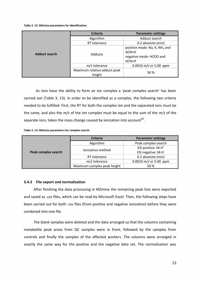
3.4.2.6 Identification
This identification step consisted of two individual tasks, the ‘adduct search’ and the
‘peak complex search’. The adduct search function in MZmine aims to find possible
predefined adducts in the peak list, e.g. formate or solvent adducts (Table 3. 12). Adducts
have been identified by two important criteria. Criterion 1 requests that the mass difference
between the adduct and the original ion must be equal to one of the chosen adducts and
criterion 2 requests that the RT of the original ion and the ion of the adduct must be the
same60.
23
Table 3. 12: MZmine parameters for identification.
After finishing the data processing in MZmine the remaining peak lists were exported
and saved as .csv files, which can be read by Microsoft Excel. Then, the following steps have
been carried out for both .csv files (from positive and negative ionization) before they were
combined into one file.
The blank samples were deleted and the data arranged so that the columns containing
metabolite peak areas from QC samples were in front, followed by the samples from
controls and finally the samples of the affected workers. The columns were arranged in
exactly the same way for the positive and the negative data set. The normalization was
24
performed by dividing the peak area of a certain metabolic feature by the sum of peak areas
for all the features in one sample.
The positive and the negative data set were finally combined and subjected to
multivariate statistical analyses.
3.5 DATA ANALYSIS
The software Simca (version 14, Umetrics, Umeå, Sweden) was used for the multivariate
statistical analyses (MVA) of the data sets obtained from HILIC-HRMS and RP-HPLC-HRMS. By
using principal component analysis (PCA) and orthogonal partial least squares projections –
discriminant analysis (OPLS-DA), the data could be visualized and analyzed.
The transposed data table from Microsoft Excel was copied into Simca and the first row,
containing a row ID and polarity, was defined as the ‘primary ID’. The second row and the
third row, which contained information on the m/z and the RT, respectively, were defined as
secondary ID’s.
3.5.1 Principal component analysis (PCA)
For unsupervised PCA in order to reveal the total variation of the dataset, all
variables were unit variance scaled (UV), which means that all variables have been centered
and divided by its standard deviation computed around the mean61. The scores for the
affected workers, the controls and the QC samples colored differently for better
visualization.
3.5.2 Orthogonal partial least squares – discriminant analysis
Supervised discriminatory analysis was performed to reveal potential markers of
response in sewage workers relative to the control group. The variables were pareto-scaled
(Par) for OPLS-DA, which means that the variables have been centered and divided by the
square root of the standard deviation of the mean. The QC samples were excluded from the
analysis.
3.5.3 Identification of potential metabolite markers
Metabolic features that contributed most to the discrimination of the affected
sewage workers and the control group were selected from the S-plot and variable-of-
importance (VIP) plot, which visualizes and scores the contribution of the loadings (i.e.
25
metabolic features) to the OPLS-DA model (cfr. 4.3). Potential metabolic markers for which
the relative standard deviation within the QC samples or in one of the groups exceeded 30%
were excluded. A two-tailed T-test was then performed using MS Excel in order to test if the
difference of the potential metabolic marker was statistically significant, and the significance
level was set to 0.05%.
The elemental composition of the remaining potential metabolite markers was
determined in Xcalibur using both positive and negative mode data. Mass uncertainty was
set to 3 ppm and obtained elemental compositions were verified using isotope peaks.
Elements included were C, H, O, N, P, Cl, Na and S. Elemental compositions were searched
against PubChem, Chemspider, Metlin, HMDB and KEGG online databases. The identity of
potential metabolite markers was further verified from MS2 fragmentation spectra.
26
4 RESULTS AND DISCUSSION
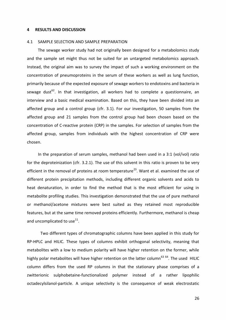
4.1 SAMPLE SELECTION AND SAMPLE PREPARATION
The sewage worker study had not originally been designed for a metabolomics study
and the sample set might thus not be suited for an untargeted metabolomics approach.
Instead, the original aim was to survey the impact of such a working environment on the
concentration of pneumoproteins in the serum of these workers as well as lung function,
primarily because of the expected exposure of sewage workers to endotoxins and bacteria in
sewage dust62. In that investigation, all workers had to complete a questionnaire, an
interview and a basic medical examination. Based on this, they have been divided into an
affected group and a control group (cfr. 3.1). For our investigation, 50 samples from the
affected group and 21 samples from the control group had been chosen based on the
concentration of C-reactive protein (CRP) in the samples. For selection of samples from the
affected group, samples from individuals with the highest concentration of CRP were
chosen.
In the preparation of serum samples, methanol had been used in a 3:1 (vol/vol) ratio
for the deproteinization (cfr. 3.2.1). The use of this solvent in this ratio is proven to be very
efficient in the removal of proteins at room temperature23. Want et al. examined the use of
different protein precipitation methods, including different organic solvents and acids to
heat denaturation, in order to find the method that is the most efficient for using in
metabolite profiling studies. This investigation demonstrated that the use of pure methanol
or methanol/acetone mixtures were best suited as they retained most reproducible
features, but at the same time removed proteins efficiently. Furthermore, methanol is cheap
and uncomplicated to use11.
Two different types of chromatographic columns have been applied in this study for
RP-HPLC and HILIC. These types of columns exhibit orthogonal selectivity, meaning that
metabolites with a low to medium polarity will have higher retention on the former, while
highly polar metabolites will have higher retention on the latter column63 64. The used HILIC
column differs from the used RP columns in that the stationary phase comprises of a
zwitterionic sulphobetaine-functionalized polymer instead of a rather lipophilic
octadecylsilanol-particle. A unique selectivity is the consequence of weak electrostatic
27
interactions between the sulphobetaine-stationary phase and polar analytes. This type of
column fits excellent for highly polar compounds, which are barely retained on the RP
column65. Thus, HILIC has the advantage of improving the retention of hydrophilic
compounds64 66.
The first set of samples, which has been applied for the HILIC column, was ready for
use after the deproteinization step (cfr. 3.2.1). For this type of column, a high level of organic
solvent was needed in order to get better separation and better peak shapes. Thus, the
methanol present in these samples, didn’t need to be evaporated. Given that a RP column
has been used for the other set of samples, these samples needed to be highly aqueous on
the contrary. Therefore, this set required some additional steps to remove the methanol and
to resolve the content in an aqueous solvent.
Besides the preparation of two different sample sets for the two chromatographic
approaches, also a QC sample (i.e. Quality Control) and a blank sample were prepared both
for HILIC-HRMS as well as RP-HPLC-HRMS. The purpose of the blank samples was their use
for the identification of “background features“, while the purpose of the QC samples was to
monitor instrumental drift. In this study, the QC sample has been a pooled QC, and the use
of this kind of QC is favorable due to its high appropriateness, but yet might not always be
possible to include in a metabolomics study23 67. A pooled QC contains an aliquot of each
test sample, and for that reason it represents more or less an average of the composition of
all the test samples, both qualitatively and quantitatively23 67.
In untargeted metabolomics studies, just like this one, the QC samples are principally
used to evaluate the potential drift of the instrument68. Another important reason for the
utilization of QC’s is that they could be implemented at the start of the batch in order to
condition the analytical platform23 68 69.
4.2 LC-HRMS ANALYSES AND DATA PROCESSING
In this investigation, two different types columns with different selectivity have been
applied in order to achieve chromatographic separation for a wide range of metabolites. As
already mentioned in section 4.1, the applicability of RP-HPLC is limited for highly polar
compounds. However, biological fluids such as serum contain polar compounds, e.g. amino
acids and carnitines, that will be better retained by HILIC63 64 70. In fact, RP-HPLC was
28
originally widely used in connection with HRMS, but recently the use of HILIC gains more
interest as the selection of stationary phases increases70 71.
Serum samples are a complex mixture of different types of compounds. This means
that good separation of all these compounds with different polarities can’t take place in an
isocratic mode. Therefore, HPLC has been used with a multi-step gradient mode for both
types of columns. The multi-step gradient for the HILIC column (cfr. 3.3.3) started with a high
proportion of organic mobile phase, and the proportion of aqueous mobile phase was
gradually increased in the course of the chromatographic run. In case of the RP-HPLC, the
gradient started with a high proportion of aqueous mobile phase (cfr. 3.3.2), while the
proportion of organic mobile phase was gradually increased in the course of the
chromatographic run.
Using an untargeted LC-HRMS approach yields a very high number of potential
metabolic features. It is impossible to handle such a high number of features manually.
MZmine typically extracted more than 10,000 potential metabolic features from the raw
data. During the processing this number was reduced to about 1,500 features. The data
processing itself is explained in section 3.4.2. One of the final steps of the processing is an
alignment step. This enabled the direct comparison of samples within one method. An
example of an aligned and gap filled peak list is shown in Figure 3. 4.
The principal aim with the normalization of data (cfr. 3.4.3), prior to multivariate
statistical analysis (MVA), was to correct for the observed instrumental drift (cfr. 4.6).
4.3 MULTIVARIATE DATA ANALYSES
The data set was visualized and analyzed by unsupervised principal component analysis
(PCA) and supervised orthogonal partial least squares projections – discriminant analysis
(OPLS-DA). These techniques offer dimension reduction and reveal associations between
data6 64. This section is based on the analysis of the original raw data set from HPLC-HRMS
analyses performed at the University of Strathclyde, Glasgow.
The first step was the visualization of data sets in unit-variance scaled PCA score scatter
plots (Figure 4. 1 and Figure 4. 2). It was not possible to observe any clear separation
between the affected and the control samples in the PCA plots including PC1 and PC2 (Figure
29
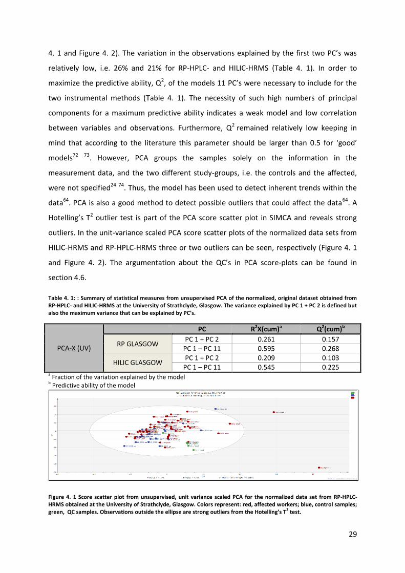
4. 1 and Figure 4. 2). The variation in the observations explained by the first two PC’s was
relatively low, i.e. 26% and 21% for RP-HPLC- and HILIC-HRMS (Table 4. 1). In order to
maximize the predictive ability, Q2, of the models 11 PC’s were necessary to include for the
two instrumental methods (Table 4. 1). The necessity of such high numbers of principal
components for a maximum predictive ability indicates a weak model and low correlation
between variables and observations. Furthermore, Q2 remained relatively low keeping in
mind that according to the literature this parameter should be larger than 0.5 for ‘good’
models72 73. However, PCA groups the samples solely on the information in the
measurement data, and the two different study-groups, i.e. the controls and the affected,
were not specified24 74. Thus, the model has been used to detect inherent trends within the
data64. PCA is also a good method to detect possible outliers that could affect the data64. A
Hotelling’s T2 outlier test is part of the PCA score scatter plot in SIMCA and reveals strong
outliers. In the unit-variance scaled PCA score scatter plots of the normalized data sets from
HILIC-HRMS and RP-HPLC-HRMS three or two outliers can be seen, respectively (Figure 4. 1
and Figure 4. 2). The argumentation about the QC’s in PCA score-plots can be found in
section 4.6.
Table 4. 1: : Summary of statistical measures from unsupervised PCA of the normalized, original dataset obtained from RP-HPLC- and HILIC-HRMS at the University of Strathclyde, Glasgow. The variance explained by PC 1 + PC 2 is defined but also the maximum variance that can be explained by PC’s.
PCA-X (UV)
PC R2X(cum)a Q2(cum)b
RP GLASGOW PC 1 + PC 2 0.261 0.157
PC 1 – PC 11 0.595 0.268
HILIC GLASGOW PC 1 + PC 2 0.209 0.103
PC 1 – PC 11 0.545 0.225 a Fraction of the variation explained by the model
b Predictive ability of the model
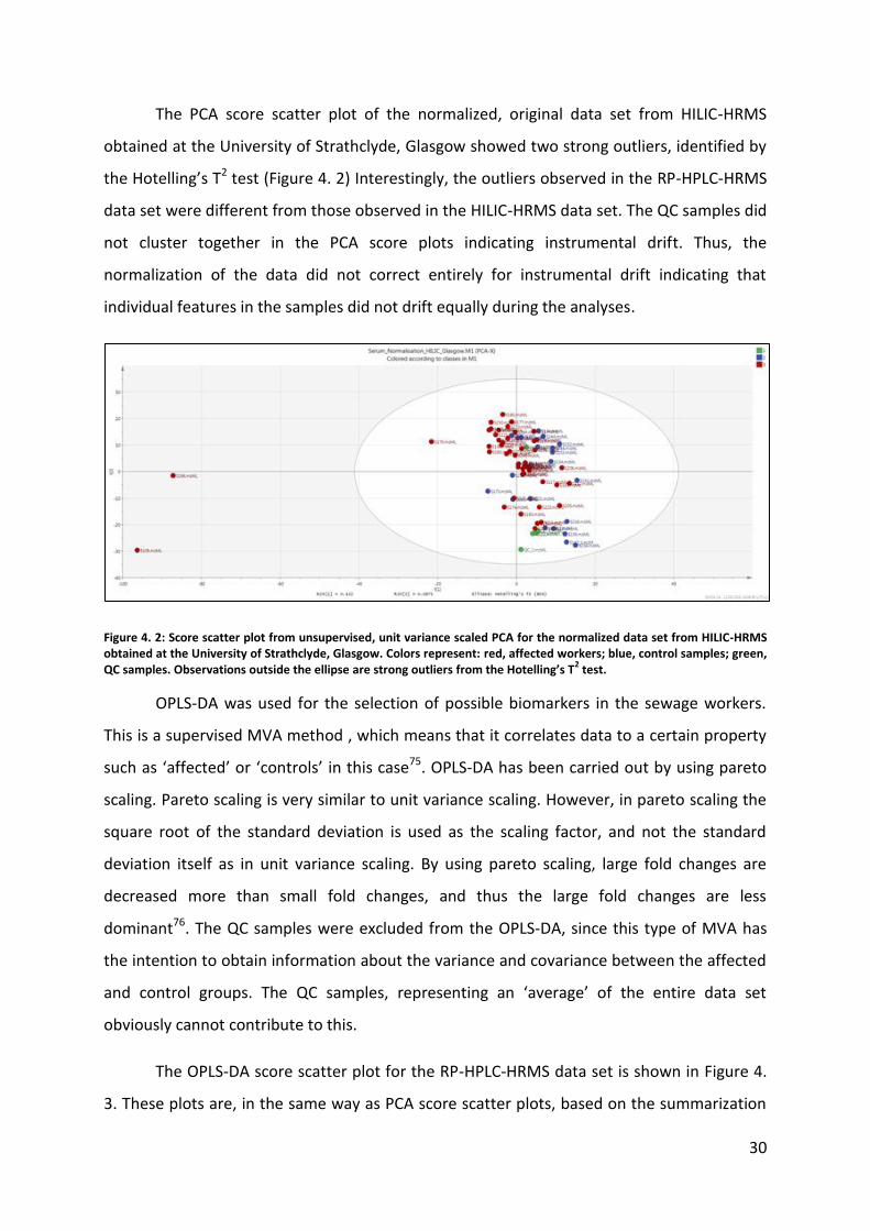
Figure 4. 1 Score scatter plot from unsupervised, unit variance scaled PCA for the normalized data set from RP-HPLC-HRMS obtained at the University of Strathclyde, Glasgow. Colors represent: red, affected workers; blue, control samples; green, QC samples. Observations outside the ellipse are strong outliers from the Hotelling’s T
2 test.
30
The PCA score scatter plot of the normalized, original data set from HILIC-HRMS
obtained at the University of Strathclyde, Glasgow showed two strong outliers, identified by
the Hotelling’s T2 test (Figure 4. 2) Interestingly, the outliers observed in the RP-HPLC-HRMS
data set were different from those observed in the HILIC-HRMS data set. The QC samples did
not cluster together in the PCA score plots indicating instrumental drift. Thus, the
normalization of the data did not correct entirely for instrumental drift indicating that
individual features in the samples did not drift equally during the analyses.
Figure 4. 2: Score scatter plot from unsupervised, unit variance scaled PCA for the normalized data set from HILIC-HRMS obtained at the University of Strathclyde, Glasgow. Colors represent: red, affected workers; blue, control samples; green, QC samples. Observations outside the ellipse are strong outliers from the Hotelling’s T
2 test.
OPLS-DA was used for the selection of possible biomarkers in the sewage workers.
This is a supervised MVA method , which means that it correlates data to a certain property
such as ‘affected’ or ‘controls’ in this case75. OPLS-DA has been carried out by using pareto
scaling. Pareto scaling is very similar to unit variance scaling. However, in pareto scaling the
square root of the standard deviation is used as the scaling factor, and not the standard
deviation itself as in unit variance scaling. By using pareto scaling, large fold changes are
decreased more than small fold changes, and thus the large fold changes are less
dominant76. The QC samples were excluded from the OPLS-DA, since this type of MVA has
the intention to obtain information about the variance and covariance between the affected
and control groups. The QC samples, representing an ‘average’ of the entire data set
obviously cannot contribute to this.
The OPLS-DA score scatter plot for the RP-HPLC-HRMS data set is shown in Figure 4.
3. These plots are, in the same way as PCA score scatter plots, based on the summarization
31
of observations77. The plot shows some separation between both groups. However, from the
plot it can also be seen that the differentiation between the groups was not complete. This
indicated a weak model which was further confirmed by the following statistical measures:
The model explained 48.6 percent of the variation between both groups (i.e.
R2Y(cum))(Table 4. 2). However, a negative number for the predictive ability of the model,
Q2, shows an especially poor fit and any identification of putative marker metabolites based
on the model must be handled with care77.
Figure 4. 3 Score scatter plot from supervised OPLS-DA (pareto scaling) of the observations from RP-HPLC-HRMS performed at the University of Strathclyde, Glasgow. Colors represent: blue, affected workers; green, control samples.
The OPLS-DA score scatter plot for the HILIC-HRMS data set is shown in Figure 4. 4. At
first sight, this looks slightly better than the same score scatter plot from the RP-HPLC-HRMS
data set. Table 4. 2, showing selected statistical measures of the model supports that this
model is significantly stronger than the above, as indicated by a higher R2Y(cum). Also, the
higher predictive ability of the model, Q2, and thus the smaller difference between Q2 and
R2Y(cum) support a stronger model.
Figure 4. 4: Score scatter plot from supervised OPLS-DA (pareto scaling) of the observations from RP-HILIC-HRMS performed at the University of Strathclyde, Glasgow. Colors represent: blue, affected workers; green, control samples.
32
Exclusion of the outliers in RP-HPLC-HRMS (S114, S146, 02_S127) and HILIC-HRMS
(S196, S109) based on the PCA plots, resulted in slightly better values for R2X, R2Y and Q2
(Table 4. 2). In the first case, observing an improvement for the negative predictive ability of
the model, but the fit still remains very weak. In HILIC-HRMS, also an increase could have
been noticed, but in this case an extra component had been included to achieve the
maximizing of the Q2. In general, this correction resulted in an insignificant small
improvement and even more, new outliers were revealed in the new score-plots.
Investigation of the S-plots, corrected for the outliers, did not change the selection of
putative biomarkers for further identification. Therefore, there had been continued with the
complete sample set.
Table 4. 2: Comparison of statistical measures for supervised OPLS-DA models obtained from RP-HPLC-HRMS and HILIC-HRMS data sets obtained at the University of Strathclyde, Glasgow.
OPLS-DA (PAR)
PC R2X(cum)a R2Y(cum)b Q2(cum)c
RP GLASGOW PC 1 + PC 2 0.237 0.486 -0.0344 RP GLASGOW
adjusted for outliers PC 1 + PC 2 0.243 0.512 0.0236
HILIC GLASGOW
PC 1 + PC 2 0.220 0.589 0.302
HILIC GLASGOW
adjusted for outliers PC 1 – PC 3 0.262 0.831 0.356
a Fraction of the variation explained by the model
b Fraction of the variation between both groups explained by the model
c Predictive ability of the model
In order to select putative metabolic markers of exposure, the S-plots for both OPLS-
DA models were studied77. An S-plot is a loadings plot visualizing and scoring the variables
(i.e. metabolic features) according to their significance for the model77. S-plots have been
constructed out of the pareto scaled OPLS-DA models. The potential metabolic markers of
exposure were selected according to their location in the S-plot (Figure 4. 5 and Figure 4. 6).
This type of loadings plot combines the modelled covariance (p[1]-axis) and the modelled
correlation (p(corr)[1]-axis) from OPLS-DA77. Putative biomarker molecules are characterized
by large variable magnitude and good reliability, and in an S-plot such variables are located
at the bottom left or upper right corner of the plot (Figure 4. 5 and Figure 4. 6)77.
33
Figure 4. 5: S-plot of supervised, pareto scaled OPLS-DA of RP-HPLC-HRMS profiled serum samples run at the University of Strathclyde, Glasgow. The blue and red colored loadings correspond to potential marker metabolites that were selected for T-testing and tentative identification.
Figure 4. 6: S-plot of supervised, pareto scaled OPLS-DA of HILIC-HRMS profiled serum samples run at the University of Strathclyde, Glasgow. The blue and red colored loadings correspond to potential marker metabolites that were selected for T-testing and tentative identification .
Figure 4. 7: Variable Importance Plot (VIP) of supervised, pareto scaled OPLS-DA of RP-HPLC-HRMS profiled serum samples run at the University of Strathclyde, Glasgow. Coloration of variables is according to the S-plot.
34
The Variable Importance Plot (VIP) is a scoring feature of the SIMCA software that
allows verifying the selection of potential metabolite markers from the S-plot. The higher the
VIP score (>1) the more significant is the metabolic feature in complex analysis in comparing
the difference between the two groups. The VIP plot is a coefficient plot that summarizes
the relationship between the X and Y variables, but the algorithm is not known (Figure 4. 7
and Figure 4. 8)78.
Figure 4. 8: Variable Importance Plot (VIP) of supervised, pareto scaled OPLS-DA of RP-HPLC-HRMS profiled serum samples run at the University of Strathclyde, Glasgow. Coloration of variables is according to the S-plot.
4.4 SELECTION OF POTENTIAL METABOLOMIC MARKERS OF EXPOSURE
The selected features from supervised OPLS-DA were tested for statistical significance
using a two-tailed T-test in excel. The statistical significant (P<0.05) potential metabolic
markers are summarized as m/z and retention time pairs in Table 4. 3 and Table 4. 4
together with their group ratio, as well as the relative standard deviation (RSD) of the
metabolic features in the QC samples and within the two groups. The ratio demonstrates
either upregulation (>1) or downregulation (<1) of the metabolite in the control vs. the
affected group. Features with a poor repeatability, i.e. features with RSD’s > 30 % in the
QC’s were removed. However, where the same feature was identified as a statistically
significant putative metabolic marker in the re-analyses carried out at STAMI, Oslo, it was
not rejected from the original (i.e. University of Strathclyde) list of metabolic markers, even
though they had RSD’s > 30 %.
35
Table 4. 3: Putative metabolic markers selected from the RP-HPLC-HRMS data set.
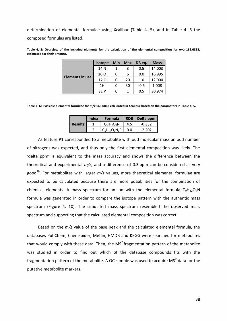
determination of elemental formulae using Xcalibur (Table 4. 5), and in Table 4. 6 the
composed formulas are listed.
Table 4. 5: Overview of the included elements for the calculation of the elemental composition for m/z 166.0862, estimated for their amount.
Elements in use
Isotope Min Max DB eq. Mass
14 N 1 3 0.5 14.003
16 O 0 6 0.0 16.995
12 C 0 20 1.0 12.000
1H 0 30 -0.5 1.008
31 P 0 1 0.5 30.974
Table 4. 6: Possible elemental formulae for m/z 166.0862 calculated in Xcalibur based on the parameters in Table 4. 5.
As feature P1 corresponded to a metabolite with odd molecular mass an odd number
of nitrogens was expected, and thus only the first elemental composition was likely. The
‘delta ppm’ is equivalent to the mass accuracy and shows the difference between the
theoretical and experimental m/z, and a difference of 0.3 ppm can be considered as very
good79. For metabolites with larger m/z values, more theoretical elemental formulae are
expected to be calculated because there are more possibilities for the combination of
chemical elements. A mass spectrum for an ion with the elemental formula C9H12O2N
formula was generated in order to compare the isotope pattern with the authentic mass
spectrum (Figure 4. 10). The simulated mass spectrum resembled the observed mass
spectrum and supporting that the calculated elemental composition was correct.
Based on the m/z value of the base peak and the calculated elemental formula, the
databases PubChem, Chemspider, Metlin, HMDB and KEGG were searched for metabolites
that would comply with these data. Then, the MS2 fragmentation pattern of the metabolite
was studied in order to find out which of the database compounds fits with the
fragmentation pattern of the metabolite. A QC sample was used to acquire MS2 data for the
putative metabolite markers.
Results
Index Formula RDB Delta ppm
1 C9H12O2N 4.5 -0.332
2 C5H15O2N2P 0.0 -2.202
39
Figure 4. 10: Isotope pattern of generated elemental composition (above) compared to isotope pattern of metabolite with m/z 166.0862 (below). The patterns are very similar.
The databases gave several suggestions for the structure of the metabolite e.g.
phenylalanine, benzocaine, 3 amino-phenylpropionic acid (which would be identical to
phenylalanine) etc. The ring double bond equivalent (RDB) of the neutral equivalent of P1
was 5 (cfr. Table 4. 6) suggested that the molecule could have a benzene ring and a carbonyl
group as in phenylalanine. Examination of the fragmentation spectrum revealed a major
product ion at m/z 120, corresponding to loss of 46 Da, and a minor product ion at m/z 149
(Figure 4. 11). The −46 Da loss, attributed to loss of the carboxyl group as formic acid, which
is diagnostic for the presence of a carboxylic acid. (Figure 4. 11). The latter product ion can
be explained by the presence of an amine function in the structure.
For all other final putative metabolic markers the chromatograms, mass spectra and
MS2 product ion spectra are shown in the appendix. However, the obtained mass spectral
data for the remaining putative metabolic markers will be briefly discussed in the following
QC8#143-166 RT: 1.44-1.65 AV: 12 T: FTMS + p ESI Full ms [80.00-1200.00]
40
Figure 4. 11: Product ion spectrum from HILIC-ion trap mass spectrometry and possible explanation for the observed product ions for the metabolite with m/z 166.0862, tentatively identified as phenylalanine.
Another metabolic feature, which was identified as a putative metabolic marker
afforded negatively charged ions with m/z 167.0213. Provided this m/z corresponds to the
deprotonated molecular ions the metabolite contains an even number of nitrogen atoms, if
any. However, the mass spectrum was noisy, and it was therefore difficult to identify an
isotope pattern (Figure 7. 1). Furthermore, the elemental formulae returned from
calculations made in Xcalibur were meaningless, and the MS2 product ion spectrum showed
only two ions corresponding to loss of 43 and 44 Da (Figure 7. 2). Thus, the compound
remained unidentified.
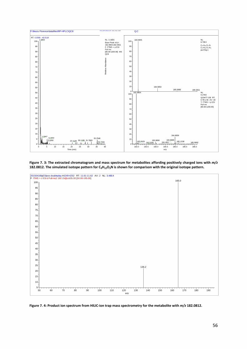
The elemental formula C9H12O3N was found to be the most likely for the metabolite
affording positively charged ions with m/z 182.0812 (Table 4. 7). The elemental composition
differed by one oxygen atom to that of the tentatively identified phenylalanine. The MS2
product ion spectrum was likewise similar and showed product ions corresponding to losses
of 17 and 46 Da (Figure 7. 4). These product ions are likely the result of loss of ammonia and
formic acid indicating the presence of amine and carboxylic acid functions. It is thus most
likely that m/z 182.0812 is equivalent to the amino acid tyrosine (4 hydroxy-phenylalanine).
41
The metabolic features m/z 311.1406 and m/z 313.1544 from negative and positive
ionization, respectively, eluted at the same retention time from the RP-HPLC columns (Table
4. 7). The calculated elemental compositions for the two ions were C18H19N2O3 and
C18H21N2O3 showing that the ions were the deprotonated and protonated molecular ions,
respectively. Database searches suggested a phenylalanine-phenylalanine dipeptide for the
elemental formulae. Several of the product ions observed in the MS2 product ion spectrum
supported a phenylalanine dipeptide (Figure 7. 6). For example, the m/z 147 product ion is
likely due to cleavage of the amide linkage between the monomers, and the m/z 164
product ion could arise from fragmentation of the bond on the other side of the amide
linkage resulting in a phenylalanine-amide (Figure 7. 6).
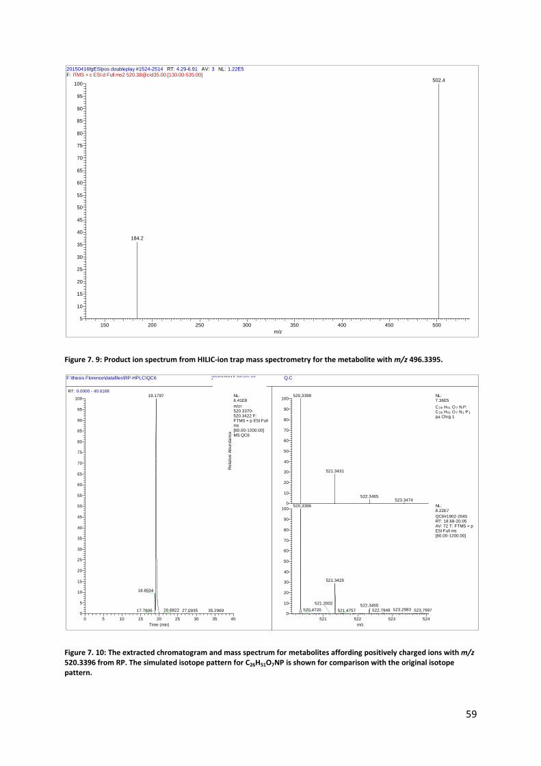
Compound 496.3395 was tentatively identified as 2- or 3-hydroxy-palmitoyl-
glycerophosphocholine (C24H51O7NP) from database searches. First, the formula had been
generated by including at least one nitrogen and no chlorine in the calculations as a result of
observations of the isotope pattern and the molecular mass indicating the presence of an
odd number of nitrogen atoms. The MS2 product ion spectrum showed a major product ion
with m/z 184 likely corresponding to a phosphocholine moiety verifying a phosphocholine-
type phospholipid (Figure 7. 9). Whether the molecule is a 2- or 3-hydroxy compound can
only be found out by comparison to authentic standards.
The m/z 520.3396 metabolic feature was significantly different between the affected
and control workers in both the RP and the HILIC approach from the samples run at the
University of Strathclyde, Glasgow. Calculating the elemental composition revealed
C26H51O7NP as the most probable elemental formula, and again sn-glycero-3-phosphocholine
molecules were suggested in the databases. The elemental composition differed by C2 to a
putative hydroxy-palmitoyl-glycerophosphocholine. The fragmentation pattern showed the
same characteristics as for previous compound (Figure 7. 12), and it could therefore be
concluded that this compound is a similar phospholipid with a longer fatty acid chain. Thus,
m/z 520.3396 is probably a 2- or 3-hydroxy-octadecadienoylglycerophosphocholine.
42
Table 4. 7: Overview of the final potential metabolic markers from untargeted RP-HPLC- and HILIC-HRMS based metabolomics and tentative identification of metabolites based on calculation of the elemental composition and study of MS2 product ion spectra. Superscripts for row m/z mean: 1: significant features from both the RP-HPLC- and HILIC data set from Glasgow, 2: significant features from the RP-HPLC data set with inter-group RSD >30%, but which were identified both in Glasgow and in Oslo, 3: significant features from the HILIC data set both from Glasgow and Oslo, 4: significant feature from HILIC and RP-HPLC data sets from Glasgow and HILIC data set from Oslo.
a The ring double bond equivalent is for the neutral molecule.
43
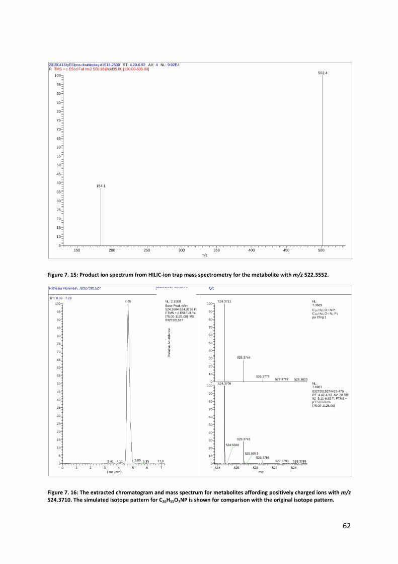
The metabolic feature with m/z 522.3552 was also present in both the RP and the
HILIC approach from the samples run at the University of Strathclyde, Glasgow.
Furthermore, the extracted ion chromatograms showed two closely eluting isomers that
were significantly different between the affected and control workers in both RP-HPLC-
HRMS data sets (Glasgow and Oslo). The calculated elemental formula for m/z 522.3552
(C26H53O7NP) showed that this metabolite contained two hydrogen atoms more than m/z
520.3396, while its MS2 product ion spectrum showed that it was a phosphocholine (Figure
7. 15). This means that the fatty acid chain of the phospholipids likely contained a mono-
unsaturated hydrocarbon chain, and thus was likely a 2- and 3-hydroxy-
octadecenoylglycerophosphocholine.
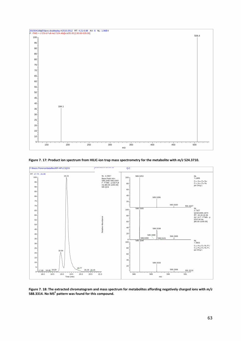
The MS characteristics for m/z 524.3710 were similar to the latter two, and its
elemental formula (C26H55O7NP) again indicated the presence of two additional hydrogen
atoms relative to m/z 522.3552 (Figure 7. 17). Thus, this metabolite was likely a 2- or 3-
hydroxy-octadecanoylglycerophosphocholine.
The most likely elemental composition for m/z 588.3314 was C24H48O4N9P2. The databases
did not contain any metabolite with this elemental composition. It was thus not possible to
come up with a suggestion for a structure of this compound.
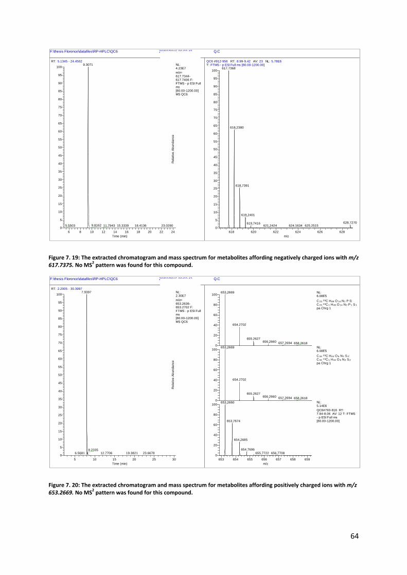
For the metabolic features m/z 617.7375 and 653.2669, observed in the negative
ionization mode, no meaningful elemental formulae were found. Both molecules were
doubly charged as can be seen from their isotope pattern (Figure 7. 19 and Figure 7. 20)80.
Thus, these metabolites were of high molecular mass allowing for many possible
combinations of chemical elements. The data-dependent scanning did not yield MS2 product
ion spectra for these two metabolic features. Therefore, the identity of these two features
remained unknown.
The 1083.6634 compound wasn’t identified either. This molecule was very large and
therefore there are a lot possible elemental compositions that would fit with the mass
spectra. Since there was no remarkable characteristic in the mass spectrum, there was no
possibility to eliminate elements to include for the elemental composition. Either no
fragmentation spectrum had been found for this molecule.
44
All these observations already gave a thought about the structures of the tentative
biomarkers. Nevertheless, further verification is needed to prove that the findings are
effective. Therefore, the standards of these discovered metabolites should have ordered and
comparisons between the mass spectra and fragmentation patterns of those and the original
ones should have been carried out to make a conclusion. In this case it’s only possible to
demonstrate which compounds they most likely are but no further conclusion could have
been made.
4.6 INSTRUMENTAL DRIFT AND REPRODUCIBILITY
In the beginning, analysis of data had been carried out on the data acquired from the
samples made in Oslo. During the investigation, the decision was made to focus on the
analysis of data found at the University of Strathclyde, Glasgow. Even though both data sets
were subjected to drift, the Oslo samples went unfortunately through two redundant freeze-
thaw-cycles before sample preparation. Suggesting that these data was less trustworthy for
the objective to detect changes in the metabolome compared to data from Glasgow.
Instrumental drift is a typical phenomenon and a major confounding factor in long-term
metabolomics investigations23. Instrumental instability results in poor data quality,
consequently complicating comparison of data between different laboratories or data
collected over time. Drift can also be encountered in the same run81. Principally, this drift is
caused by samples coming into direct contact with components of the analytical platform.
This can lead to changes in retention times and measured response over time by
contaminating or dirtying of the ion source and by changes in chromatographic performance
such as column aging81 82. Increasing analysis times generally lead to increasing drift81.
In order to deal with this drift, normalization of all data sets had been carried out to
improve reproducibility. After these normalization, there could be deduced with the help
from the QC’s that the data sets were still subjected to some instrumental drift. Since both
Oslo and Glasgow data sets were still dominated by this drift after normalization, the
acquired results should be handled cautiously.
The use of PCA score-plots was very useful to acquire practical information about the
QC samples and in general about the instrumental drift. When having a look at the RP PCA
score-plot for samples made in Oslo (Figure 4. 12), there could be noticed that QC1, QC2,
45
QC3 and QC4, were located very far from the other QC’s but in general very far from all
other samples. They were even detected as strong outliers. Another remarkable thing was
that they weren’t clustered. Ideally, the QC samples should have been grouped as a cluster
in the plot, because they all derive from the same vial and thus hold the same content23 67 68.
In section 4.1, there had been described that QC’s are implemented at the start of the batch
in order to condition the analytical platform and counteract for the drift. This was the fact in
our case and is probably the reason why the first QC’s are dispersed and isolated from the
others. Therefore QC1 until 4 could have been excluded68 69.
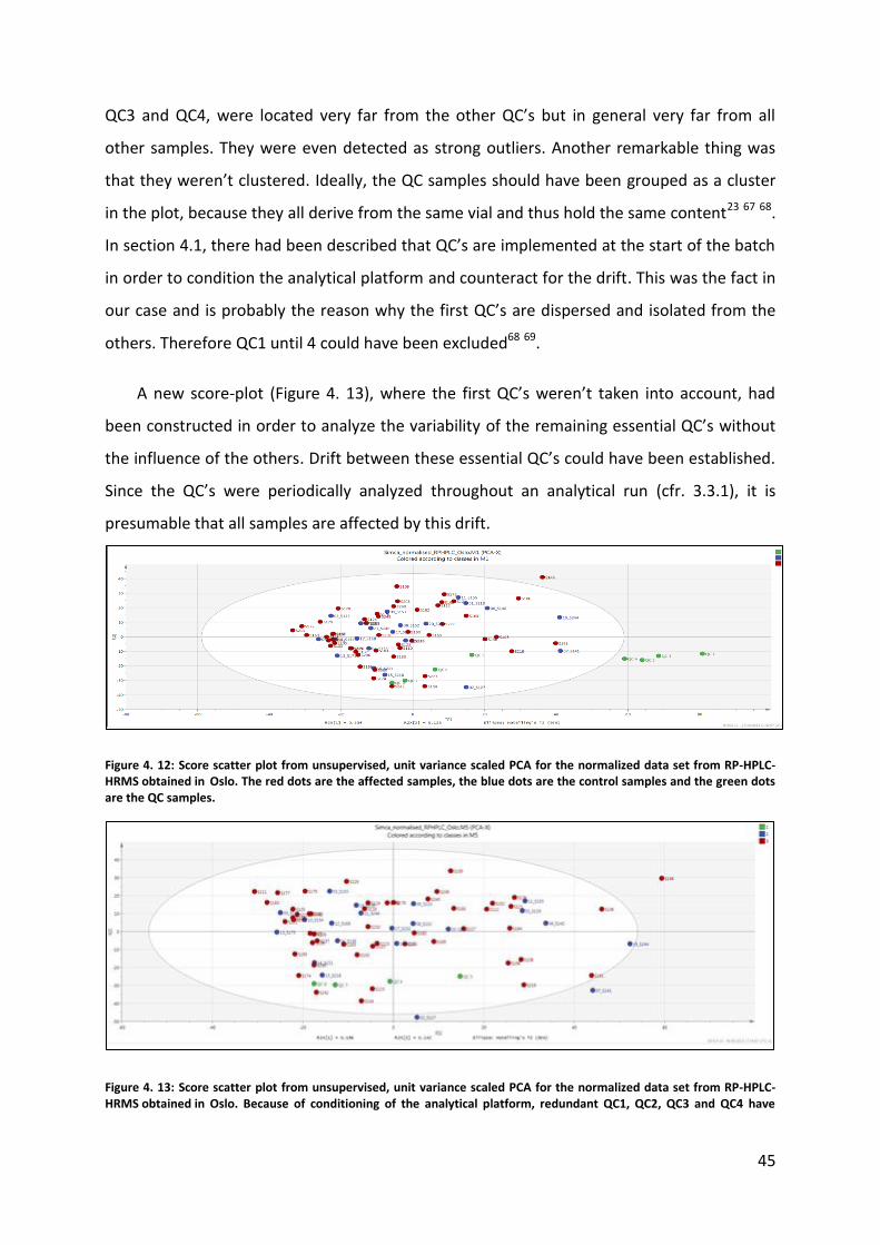
A new score-plot (Figure 4. 13), where the first QC’s weren’t taken into account, had
been constructed in order to analyze the variability of the remaining essential QC’s without
the influence of the others. Drift between these essential QC’s could have been established.
Since the QC’s were periodically analyzed throughout an analytical run (cfr. 3.3.1), it is
presumable that all samples are affected by this drift.
Figure 4. 12: Score scatter plot from unsupervised, unit variance scaled PCA for the normalized data set from RP-HPLC-HRMS obtained in Oslo. The red dots are the affected samples, the blue dots are the control samples and the green dots are the QC samples.
Figure 4. 13: Score scatter plot from unsupervised, unit variance scaled PCA for the normalized data set from RP-HPLC-HRMS obtained in Oslo. Because of conditioning of the analytical platform, redundant QC1, QC2, QC3 and QC4 have
46
been excluded. The red dots are the affected samples, the blue dots are the control samples and the green dots are the QC samples.
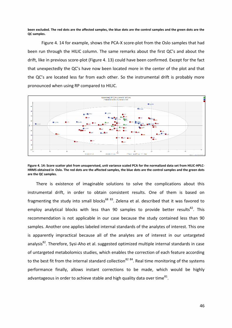
Figure 4. 14 for example, shows the PCA-X score-plot from the Oslo samples that had
been run through the HILIC column. The same remarks about the first QC’s and about the
drift, like in previous score-plot (Figure 4. 13) could have been confirmed. Except for the fact
that unexpectedly the QC’s have now been located more in the center of the plot and that
the QC’s are located less far from each other. So the instrumental drift is probably more
pronounced when using RP compared to HILIC.
Figure 4. 14: Score scatter plot from unsupervised, unit variance scaled PCA for the normalized data set from HILIC-HPLC-HRMS obtained in Oslo. The red dots are the affected samples, the blue dots are the control samples and the green dots are the QC samples.
There is existence of imaginable solutions to solve the complications about this
instrumental drift, in order to obtain consistent results. One of them is based on
fragmenting the study into small blocks68 83. Zelena et al. described that it was favored to
employ analytical blocks with less than 90 samples to provide better results82. This
recommendation is not applicable in our case because the study contained less than 90
samples. Another one applies labeled internal standards of the analytes of interest. This one
is apparently impractical because all of the analytes are of interest in our untargeted
analysis82. Therefore, Sysi-Aho et al. suggested optimized multiple internal standards in case
of untargeted metabolomics studies, which enables the correction of each feature according
to the best fit from the internal standard collection82 84. Real time monitoring of the systems
performance finally, allows instant corrections to be made, which would be highly
advantageous in order to achieve stable and high quality data over time81.
47
5 CONCLUSION
In this study, 13 different metabolites have been revealed as potential metabolic
markers in sewage workers by comparing serum samples with a control group based on an
untargeted HPLC-HRMS metabolomics approach. This study thus also demonstrated the
potential of this technique for research in occupational health.
The major problem encountered was related to the presence of instrumental drift. Even
though efforts were done to counteract for this instrumental drift such as including a pre-
run for instrument equilibration and normalization of the raw data, the insurmountable
occurrence of instrumental drift, could not entirely be avoided nor corrected for. This is
likely the principal reason for the observed inconsistency of the results when the analyses
were repeated. Future research should thus focus on minimizing the problems related to
instrumental drift. Since the potential metabolic markers have solely been identified
tentatively the identity of their structures still needs be compared with authentic standards.
48
6 BIBLIOGRAPHY
1. Fiehn O. Metabolomics - The link between genotypes and phenotypes. Plant Mol Biol. 2002;48(1-2):155-171.
2. Griffiths WJ, Karu K, Hornshaw M, Woffendin G, Wang Y. Metabolomics and metabolite profiling: past heroes and future developments. Eur J Mass Spectrom (Chichester, Eng). 2007;13(1):45-50.
3. Vulimiri S V, Pachkowski B, Bale AS, Sonawane B. Metabolomics Approach for Hazard Identification in Human Health Assessment of Environmental Chemicals. Metabolomics. 2012:349-364.
4. Dunn WB, Ellis DI. Metabolomics: Current analytical platforms and methodologies. TrAC - Trends Anal Chem. 2005;24(4):285-294.
5. Jewett JN and MC. The role of metabolomics in systems biology. Stress Protein Kinases. 2008;20(August 2007):51-79.
6. Dettmer K, Aronov P a, Hammock BD. Mass spectrometry-based metabolomics. Mass Spectrom Rev. 2007;26(1):51-78.
7. Psychogios N, Hau DD, Peng J, et al. The human serum metabolome. PLoS One. 2011;6(2).
8. Courant F, Antignac J-P, Dervilly-Pinel G, Le Bizec B. Basics of mass spectrometry based metabolomics. Proteomics. 2014;14(21-22):2369-2388.
9. Oliver SG, Winson MK, Kell DB, Baganz F. Systematic functional analysis of the yeast genome. Trends Biotechnol. 1998;16(9):373-378.
11. Want EJ, O'Maille G, Smith C a., et al. Solvent-dependent metabolite distribution, clustering, and protein extraction for serum profiling with mass spectrometry. Anal Chem. 2006;78(3):743-752.
12. Zhang A, Sun H, Wang P. et al.. Recent and potential developments of biofluid analyses in metabolomics. Journal of Proteomics 2012;75: 1079-1088.
13. Ryan D, Robards K. Metabolomics: The greatest omics of them all? Anal Chem. 2006;78(23):7954-7958.
14. Bino RJ, Hall RD, Fiehn O, et al. Potential of metabolomics as a functional genomics tool. Trends Plant Sci. 2004;9(9):418-425.
49
15. Rochfort S. Biology and Implications for Natural Products Research. 2005:1813-1820.
16. Ideker T, Galitski T, Hood L. A New Approach To Decoding L Ife: Systems Biology. Annu Rev Genomics Hum Genet. 2001;2:343-372.
17. Dettmer K, Hammock BD. Metabolomics - A new exciting field within the “omics” sciences. Environ Health Perspect. 2004;112(7):396-397.
18. Wang Z, Gerstein M, Snyder M. RNA-Seq: a revolutionary tool for transcriptomics. Nat Rev Genet. 2009;10(1):57-63.
19. Hegde PS, White IR, Debouck C. Interplay of transcriptomics and proteomics. Curr Opin Biotechnol. 2003;14(6):647-651.
20. Bensimon A, Heck AJR, Aebersold R. Mass Spectrometry–Based Proteomics and Network Biology. Annu Rev Biochem. 2012;81(1):379-405.
21. Choudhary C, Mann M. Decoding signalling networks by mass spectrometry-based proteomics. Nat Rev Mol Cell Biol. 2010;11(6):427-439.
22. Altelaar a FM, Munoz J, Heck AJR. Next-generation proteomics: towards an integrative view of proteome dynamics. Nat Rev Genet. 2013;14(1):35-48.
23. Dunn WB, David Broadhurst, Paul Begley EZ, Francis-McIntyre S, et al. Procedures for large-scale metabolic profiling of serum and plasma using gas chromatography and liquid chromatography coupled to mass spectrometry. 2011;6(7):1060-1083
24. Villas-Bôas SG, Mas S, Åkesson M, Smedsgaard J, Nielsen J. Mass spectrometry in metabolome analysis. Mass Spectrom Rev. 2005;24(5):613-646.
25. Kell DB. Systems biology, metabolic modelling and metabolomics in drug discovery and development. Drug Discov Today. 2006;11(23-24):1085-1092.
26. Mickiewicz B, Villemaire ML, Sandercock LE, Jirik FR, Vogel HJ. Metabolic changes associated with selenium deficiency in mice. Biometals. 2014:1137-1147.
27. Kume S, Yamato M, Tamura Y, et al. Potential biomarkers of fatigue identified by plasma metabolome analysis in rats. PLoS One. 2015;10(3):e0120106.
28. Zhang A, Sun H, Wang X. Serum metabolomics as a novel diagnostic approach for disease: a systematic review. 2012; 404: 1239-1245
29. Zhang T, Watson DG, Wang L, et al. Application of Holistic Liquid Chromatography-High Resolution Mass Spectrometry Based Urinary Metabolomics for Prostate Cancer Detection and Biomarker Discovery. PLoS One. 2013;8(6):1-10.
50
30. Halket JM, Waterman D, Przyborowska AM, Patel RKP, Fraser PD, Bramley PM. Chemical derivatization and mass spectral libraries in metabolic profiling by GC/MS and LC/MS/MS. J Exp Bot. 2005;56(410):219-243.
31. Lu W, Bennett BD, Rabinowitz JD. Analytical strategies for LC-MS-based targeted metabolomics. J Chromatogr B Anal Technol Biomed Life Sci. 2008;871(2):236-242.
32. Ellis DI, Dunn WB, Griffin JL, Allwood JW, Goodacre R. Metabolic fingerprinting as a diagnostic tool. Pharmacogenomics. 2007;8(9):1243-1266.
33. García-Pérez I, Vallejo M, García a., Legido-Quigley C, Barbas C. Metabolic fingerprinting with capillary electrophoresis. J Chromatogr A. 2008;1204(2):130-139.
34. Allen J, Davey HM, Broadhurst D, Rowland JJ, Oliver SG, Kell DB. Discrimination of modes of action of antifungal substances by use of metabolic footprinting. Appl Environ Microbiol. 2004;70(10):6157-6165.
35. Kell DB, Brown M, Davey HM, Dunn WB, Spasic I, Oliver SG. Metabolic footprinting and systems biology: the medium is the message. Nat Rev Microbiol. 2005;3(7):557-565.
36. Zhang A, Sun H, Wang P, Han Y, Wang X. Modern analytical techniques in metabolomics analysis. Analyst. 2012;137(2):293.
37. John C. Lindon EH and JKN. So, what’s the deal with metabolomics? Analytical Chemistry 2003:384-391
38. Spaan S, Smit L a M, Eduard W, et al. Endotoxin exposure in sewage treatment workers: investigation of exposure variability and comparison of analytical techniques. 2008:251-261.
39. Heldal KK, Madsø L, Huser PO, Eduard W. Exposure, symptoms and airway inflammation among sewage workers. 2010:263-268.
40. Douwes J, Mannetje a., Heederik D. Work-related symptoms in sewage treatment workers. Ann Agric Environ Med. 2001;8(1):39-45.
41. Gattie DK, Lewis DL. A high-level disinfection standard for land-applied sewage sludges (biosolids). Environ Health Perspect. 2004;112(2):126-131.
42. Thorn J, Beijer L, Jonsson T, Rylander R. Measurement strategies for the determination of airborne bacterial endotoxin in sewage treatment plants. Ann Occup Hyg. 2002;46(6):549-554.
43. Rylander R. Health effects among workers in sewage treatment plants. 1999:354-357.
44. Svendsen K. Dutch Expert Committee on Occupational Standards: Hydrogen Sulphide. Health Based Recommended Occupational Exposure Limit in the Netherlands.; 2001.
51
45. Weng H, Dai Z, Ji Z, Gao C, Liu C. Release and control of hydrogen sulfide during sludge thermal drying. J Hazard Mater. 2015;296:61-67.
46. Reiffenstein RJ, Hulbert WC, Roth SH. Toxicology of hydrogen sulfide. Annu Rev Pharmacol Toxicol. 1992;32(5):109-134.
47. Richardson DB. Respiratory effects of chronic hydrogen sulfide exposure. Am J Ind Med. 1995;28(1):99-108.
48. Watt MM, Watt SJ, Seaton a. Episode of toxic gas exposure in sewer workers. Occup Environ Med. 1997;54(4):277-280.
49. Thorn È. Health Effects Among Employees in Sewage Treatment Plants : A Literature Survey. 2001;179(May):170-179.
50. Heng BH, Gohr KT, Doraisingham S, Quek GH. Prevalence of hepatitis A virus infection among sewage workers in Singapore. 1994:121-128.
51. Brugha R, Heptonstall J, Farrington P, Andren S, Perry K, Parry J. Risk of hepatitis A infection in sewage workers. Occup Environ Med. 1998;55(8):567-569.
52. Grady CPL, Jr., Daigger GT, Love NG, Filipe CDM. Biological Wastewater Treatment, Third Edition.; 2011.
53. Fenn JB, Mann M, Meng CKAI, Wong SF, Whitehouse CM. Electrospray Ionization for Mass Spectrometry of Large Biomolecules. 2007: 64-71
54. Bromirski M, Exactive PM. Exactive Plus.
55. Miller PE, Denton MB. The quadrupole mass filter: Basic operating concepts. J Chem Educ. 1986;63(7):617.
56. Bharti A, Ma PC, Salgia R. Biomarker discovery in lung cancer--promises and challenges of clinical proteomics. Mass Spectrom Rev. 2008;26(3):451-466.
57. De Vos R, Moco S, Lommen A, Keurentjes J, Bino R, Hall R. Untargeted large-scale plant metabolomics using liquid chromatography coupled to mass spectrometry. 2007;2(4):778-791
58. Pluskal T, Castillo S, Villar-Briones A, Oresic M. MZmine 2: modular framework for processing, visualizing, and analyzing mass spectrometry-based molecular profile data. BMC Bioinformatics. 2010;11:395.
59. Alexandrov T, Steinhorst K. Peak detection in mass spectrometry data using sparse coding. 2008.
60. Mzmine A. About MZmine 2. 2010:1-107.
52
61. Simca manual. http://www.sartorius.com/fileadmin/media/global/products/Manual_BioPAT_SIMCA_SBI6011-e.pdf. Accessed March 12, 2015.
62. Heldal KK, Barregard L, Larsson P, Ellingsen DG. Pneumoproteins in sewage workers exposed to sewage dust. Int Arch Occup Environ Health. 2013;86(1):65-70.
63. Theodoridis G, Gika HG, Wilson ID. LC-MS-based methodology for global metabolite profiling in metabonomics/metabolomics. TrAC - Trends Anal Chem. 2008;27(3):251-260..
64. Cubbon S, Bradbury T, Wilson J, Thomas-Oates J. Hydrophilic interaction chromatography for mass spectrometric metabonomic studies of urine. 2007;79(23):8911-8918.
65. Sample Solvent and Solvent Strength ZIC - p HILIC HPLC Column General Instructions for Care and Use. 2008;49(0):6427.
66. Nguyen HP, Schug K a. The advantages of ESI-MS detection in conjunction with HILIC mode separations: Fundamentals and applications. J Sep Sci. 2008;31(9):1465-1480.
67. Dunn W, Wilson I, Nicolls A, Broadhurst D. The importance of experimental design and QC samples in large-scale and MS-driven untargeted metabolomic studies of humans. 2012;4(18):2249-2264
68. Zelena E, Dunn WB, Broadhurst D, et al. Development of a robust and repeatable UPLC-MS method for the long-term metabolomic study of human serum. Anal Chem. 2009;81(4):1357-1364.
69. Begley P, Francis-McIntyre S, Dunn WB, et al. Development and performance of a gas chromatography-time-of-flight mass spectrometry analysis for large-scale nontargeted metabolomic studies of human serum. Anal Chem. 2009;81(16):7038-7046.
70. Bharti A, Ma PC, Salgia R. Biomarker discovery in lung cancer--promises and challenges of clinical proteomics. Mass Spectrom Rev. 2010;26(3):451-466.
71. Zhang R, Watson DG, Wang L, Westrop GD, Coombs GH, Zhang T. Evaluation of mobile phase characteristics on three zwitterionic columns in hydrophilic interaction liquid chromatography mode for liquid chromatography-high resolution mass spectrometry based untargeted metabolite profiling of Leishmania parasites. J Chromatogr A. 2014;1362:168-179.
72. Eriksson L, Johansson E, Kettaneh-Wold N, Trygg C, Wikström C, Wold S. Pca. Multi- Megavariate Data Anal Part 1, Basic Princ Appl. 2006:39-62.
53
73. Triba MN, Le Moyec L, Amathieu R, et al. PLS/OPLS models in metabolomics: the impact of permutation of dataset rows on the K-fold cross-validation quality parameters. Mol BioSyst. 2015;11(1):13-19.
74. Locci E, Scano P, Rosa MF, et al. A metabolomic approach to animal vitreous humor topographical composition: a pilot study. PLoS One. 2014;9(5):e97773.
75. Jung JY, Lee HS, Kang DG, et al. 1 H-NMR-based metabolomics study of cerebral infarction. Stroke. 2011;42(5):1282-1288.
76. Van den Berg R a, Hoefsloot HCJ, Westerhuis J a, Smilde AK, van der Werf MJ. Centering, scaling, and transformations: improving the biological information content of metabolomics data. BMC Genomics. 2006;7:142.
77. Wiklund S. Multivariate Data Analysis for Omics. 2008:228.
78. Trivedi DK, Iles RK. The Application of SIMCA P+ in Shotgun Metabolomics Analysis of
ZICⓇHILIC-MS Spectra of Human Urine - Experience with the Shimadzu IT-T of and Profiling Solutions Data Extraction Software. J Chromatogr Sep Tech. 2012;03(06):145.
79. Analysis Q, Guide U. Xcalibur. 2012;(August).
80. Trauger S a., Webb W, Siuzdak G. Peptide and protein analysis with mass spectrometry. Spectroscopy. 2002;16(1):15-28.
81. Hällqvist J. Investigation of parameters causing drift in metabolomic analyzes. 2014.
82. Kamleh MA, Ebbels TMD, Spagou K, Masson P, Want EJ. Optimizing the use of quality control samples for signal drift correction in large-scale urine metabolic profiling studies. Anal Chem. 2012;84(6):2670-2677.
83. Bijlsma, S.; Bobeldijk, I.; Verheij, E. R.; Ramaker, R.; Kochhar, S.; Macdonald, I. A.; van Ommen, B.; Smilde AK. Large-Scale Human Metabolomics Studies: A strategy for Data (Pre-) Processing and Validation. 2006:567-574.
84. Sysi-Aho M, Katajamaa M, Yetukuri L, Oresic M. Normalization method for metabolomics data using optimal selection of multiple internal standards. BMC Bioinformatics. 2007;8:93.
In this part, the chromatograms, the mass spectra, the calculated mass spectra out of
the potential elemental formula and the fragmentation spectra could be found.
Figure 7. 1: The extracted chromatogram and mass spectrum for metabolites affording negatively charged ions with m/z 167.0213. For this molecule, no elemental composition has been found.
Figure 7. 2: Product ion spectrum from HILIC-ion trap mass spectrometry for the metabolite with m/z 167.0213.
Figure 7. 3: The extracted chromatogram and mass spectrum for metabolites affording positively charged ions with m/z 182.0812. The simulated isotope pattern for C9H12O3N is shown for comparison with the original isotope pattern.
Figure 7. 4: Product ion spectrum from HILIC-ion trap mass spectrometry for the metabolite with m/z 182.0812.
Figure 7. 5: The extracted chromatogram and mass spectrum for metabolites affording negatively charged ions with m/z 311.1406. The simulated isotope pattern for C18H19N2O3 is shown for comparison with the original isotope pattern.
Figure 7. 6: Product ion spectrum from HILIC-ion trap mass spectrometry for the metabolite with m/z 311.1406.
Figure 7. 7: The extracted chromatogram and mass spectrum for metabolites affording positively charged ions with m/z 313.1544. No MS
2 pattern was found for this compound. The simulated isotope patterns for different compositions have
been shown.
Figure 7. 8: The extracted chromatogram and mass spectrum for metabolites affording positively charged ions with m/z 496.3395. The simulated isotope pattern for C24H51O7NP is shown for comparison with the original isotope pattern.
Base Peak m/z= 495.8395-496.8395 F: FTMS + p ESI Full ms [75.00-1125.00] MS 0327201527
494 496 498 500 502
m/z
0
10
20
30
40
50
60
70
80
90
100
0
10
20
30
40
50
60
70
80
90
100
Re
lative
Ab
un
da
nce
496.3395
497.3427
498.3453494.3241
495.3275
499.3476 502.2923
496.3398
497.3431
498.3465499.3474 501.3541
NL:1.83E8
0327201527#427-504 RT: 4.53-5.27 AV: 39 T: FTMS + p ESI Full ms [75.00-1125.00]
NL:7.52E5
C 24 H51 O 7 NP: C 24 H51 O 7 N1 P1
pa Chrg 1
59
Figure 7. 9: Product ion spectrum from HILIC-ion trap mass spectrometry for the metabolite with m/z 496.3395.
Figure 7. 10: The extracted chromatogram and mass spectrum for metabolites affording positively charged ions with m/z 520.3396 from RP. The simulated isotope pattern for C26H51O7NP is shown for comparison with the original isotope pattern.
20150416fgESIpos doubleplay #1524-2514 RT: 4.29-6.91 AV: 3 NL: 1.22E5F: ITMS + c ESI d Full ms2 [email protected] [130.00-535.00]
m/z= 520.3370-520.3422 F: FTMS + p ESI Full ms [80.00-1200.00] MS QC6
521 522 523 524
m/z
0
10
20
30
40
50
60
70
80
90
100
0
10
20
30
40
50
60
70
80
90
100
Re
lative
Ab
un
da
nce
520.3398
521.3431
522.3465523.3474
520.3396
521.3429
522.3455523.2983520.4720 522.7948 523.7997
521.2002
521.4757
NL:7.36E5
C 26 H51 O 7 N P: C 26 H51 O 7 N1 P1
pa Chrg 1
NL:8.22E7
QC6#1902-2045 RT: 18.68-20.05 AV: 72 T: FTMS + p ESI Full ms [80.00-1200.00]
60
Figure 7. 11: The extracted chromatogram and mass spectrum for metabolites affording positively charged ions with m/z 520.3396 from HILIC. The simulated isotope pattern for C26H51O7NP is shown for comparison with the original isotope pattern.
Figure 7. 12: Product ion spectrum from HILIC-ion trap mass spectrometry for the metabolite with m/z 520.3396.
Base Peak m/z= 520.3370-520.3422 F: FTMS + p ESI Full ms [75.00-1125.00] MS 0327201527
519 520 521 522 523 524
m/z
0
10
20
30
40
50
60
70
80
90
100
0
10
20
30
40
50
60
70
80
90
100
Re
lative
Ab
un
da
nce
520.3398
521.3431
522.3465523.3474 524.3507
520.3396
522.3550524.3706
521.3428
523.3588
519.3271
520.0241
520.6513 524.0502521.6079
NL:7.36E5
C 26 H51 O7 N P: C 26 H51 O7 N1 P 1
pa Chrg 1
NL:2.12E8
0327201527#423-472 RT: 4.49-4.95 AV: 25 T: FTMS + p ESI Full ms [75.00-1125.00]
20150416fgESIpos doubleplay #1534-2528 RT: 4.29-6.92 AV: 4 NL: 9.92E4F: ITMS + c ESI d Full ms2 [email protected] [130.00-535.00]
150 200 250 300 350 400 450 500
m/z
5
10
15
20
25
30
35
40
45
50
55
60
65
70
75
80
85
90
95
100
Re
lative
Ab
un
da
nce
502.4
184.1
61
Figure 7. 13: The extracted chromatogram and mass spectrum for metabolites affording positively charged ions with m/z 522.3552 from RP. The simulated isotope pattern for C26H53O7NP is shown for comparison with the original isotope pattern.
Figure 7. 14: The extracted chromatogram and mass spectrum for metabolites affording positively charged ions with m/z 522.3555 from HILIC. The simulated isotope pattern for C26H53O7NP is shown for comparison with the original isotope pattern.
Base Peak m/z= 522.3529-522.3581 F: FTMS + p ESI Full ms [75.00-1125.00] MS 0327201527
522 523 524 525
m/z
0
10
20
30
40
50
60
70
80
90
100
0
10
20
30
40
50
60
70
80
90
100
Re
lative
Ab
un
da
nce
522.3509
523.3543
524.3552 525.3585
522.3549
524.3705
523.3587 525.3741
524.2293522.2155 522.4877 524.5029
525.2321523.2177
523.4930
NL:2.07E5
C 26 H52 O 7 N P: C 26 H52 O 7 N1 P1
pa Chrg 1
NL:1.01E8
0327201527#426-469 RT: 4.53-4.93 AV: 22 SB: 92 5.11-6.92 T: FTMS + p ESI Full ms [75.00-1125.00]
62
Figure 7. 15: Product ion spectrum from HILIC-ion trap mass spectrometry for the metabolite with m/z 522.3552.
Figure 7. 16: The extracted chromatogram and mass spectrum for metabolites affording positively charged ions with m/z 524.3710. The simulated isotope pattern for C26H55O7NP is shown for comparison with the original isotope pattern.
20150416fgESIpos doubleplay #1518-2530 RT: 4.29-6.92 AV: 4 NL: 9.92E4F: ITMS + c ESI d Full ms2 [email protected] [130.00-535.00]