ACS | Institute for Automation of Complex Power Systems ERC | E.ON Energy Research Center RWTH Aachen University Mathieustr. 6, 52074 Aachen, Germany Tel.: +49 241 80 49700 Fax.: +49 241 80 49709 [email protected]www.eonerc.rwth-aachen.de Master Thesis Analysis on Voltage Stability Indices Christine E. Doig Cardet Electrical Power Engineering Aachen, _____________ __________________________ Aachen, _____________ __________________________
Transcript
ACS | Institute for Automation of Complex Power Systems ERC | E.ON Energy Research Center RWTH Aachen University Mathieustr. 6, 52074 Aachen, Germany
I would like to express my thanks to the ACS Institute at the E.ON Research Center at RWTH Aachen and all of its members, for accepting me as a Master Thesis exchange student, letting me use their facilities and making me feel at home. Especially, I would like to thank Prof. Monti and Prof. Ponci for their valuable advice.
I am bound to thank my supervisor, Dipl.-Wirt.-Ing. Marco Cupelli, who has supported me in this thesis topic, made interesting suggestions and helped me in its development.
My special thanks go to Jungie Tang and Junqi Liu for providing me the two network systems in RTDS® as well as solving my doubts on the use of the software.
I also would like to express my thanks to all friends and colleagues in Aachen, especially Germán Díaz, who has looked after me during my stay, and Carmen, Klaus und Julia Neumann, who have always treated me as part of their family.
Last but not least, I would like to express my gratitude to my mother, father and sister, whose support has enabled me to complete this work.
2
Declaration of authorship
"I hereby declare that I have written this thesis without any help from others and without the use of documents and aids other than those stated; that I have mentioned all used sources and that I have cited them correctly according to established academic citation rules."
This thesis discusses the performance of different line voltage stability indices previously studied in literature including Lmn Index, Fast Voltage Stability Index (FVSI), Voltage Collapse Point Indicators (VCPI), and LQP Index, as well as the traditional Jacobian index based on the minimum eigenvalue of the Jacobian matrix. The indices were tested in a small 5-bus system and in a larger 39-bus system. The simulation tool used was RTDS® and the indices where computed using the control blocks components in order to monitor the values in real time. This method was chosen to have the indices values available for future control algorithm development. All the indices were found consistent with their theoretical background and the performance comparison was based on three characteristics: their accuracy, robustness to uncertainty and usable for control purposes. From the results and based on these comparison characteristics, VCPI (p) was found to have the best performance from the indices studied.
A. 39-bus system parameters ........................................................................ 101
B. Minimum eigenvalue of the Jacobian Matrix-MatLab code ........................ 103
Introduction 7
1. Introduction
In recent years, several blackouts related to voltage stability problems have occurred in many countries. In particular, 2003 was an intense year regarding blackouts with a total of 6 major ones affecting the US, the UK, Denmark, Sweden and Italy. The U.S.-Canadian blackout of August 14th, 2003 affected approximately 50 million people in eight U.S. states and two Canadian provinces. In the same year, on September 23rd 2003, the Swedish/Danish system went down affecting 2.4 million customers and five days later, September 28th, another major blackout occurred in continental Europe which resulted in a complete loss of power throughout Italy.
In order to understand why these failures are happening, it should be taken into account that nowadays power systems have to operate closer to their limits. There is an ever-increasing power demand, which could in a near future expect a higher rise with the establishment of electrical vehicles. At the same time, transmission networks are not enlarged due to economic and environmental considerations and few lines are constructed. In addition, the growing usage of renewable energy tends to make the networks more stressed, since these sources have a higher dynamic and stochastic behaviour. Finally, another factor is the liberalisation of electricity supply industry (deregulation), which has resulted in a significant increase in inter-area or cross-border trades, which are not always well accounted for when planning system security.
As mentioned above, the actual scene is no longer the same as it used to be and power systems ought to adapt to this new situation. In [1], after analysing the sequence of events that preceded these recent catastrophic failures, the following conclusion was drawn. The root causes of these blackouts were among others a shortage of reliable real-time data, no time to take decisive and suitable remedial action against unfolding events and a lack of properly automated and coordinated controls to take immediate action to prevent cascading.
Because power systems are operating closer to their limits, voltage stability assessment and control, although not a new issue, is now receiving a special attention. As defined in [2], voltage stability is the ability of a power system to maintain steady acceptable voltages at all buses in the system under normal operating conditions and after being subjected to a disturbance. The study of voltage stability can be analysed under different approaches, but specially, the assessment of how close the system is to voltage collapse can be very useful for operators. This information on the proximity of voltage instability can be given through Voltage Stability Indices. These indices can be used online to enable the operators to take action or even to automate control actions to prevent voltage collapse from happening or offline for the designing and planning stages.
Introduction 8
There are many studies on traditional Voltage Stability Indices (VSI) and some comparisons papers between them can be found in the literature, such as [9], [11]-[14] and [48]. Recently, with the development of the Phasor Measurement Units (PMU) technology, new methods are evolving to implement Wide Area Monitoring Systems (WAMSs). These new algorithms use voltages and currents provided by the PMU (synchronized to within a microsecond) to assess the stability of the power system, as in [29] and [30]-[40].
The main objective of this thesis is to describe, analyse and compare the performance of traditional Voltage Stability Indices. Simulations will be done using RTDS®, a Real-Time Digital Simulator installed at the Institute for Automation of Complex Power Systems at the E.ON Research Center at RWTH Aachen University, and two test networks: a 5-bus system and a 39-bus system. The computation of the indices will be done using RTDS® and MatLab.
The remaining of this thesis comprehends seven chapters.
Chapter 2 recalls a voltage stability overview. In this respect, basic definitions on voltage stability, a classification of instabilities and a description of different analysis methods are given.
Chapter 3 deals with traditional voltage stability indices, their classification, a presentation of some examples of each category and a comparison between them.
Chapter 4 details the methods for voltage stability assessment using PMU-based analysis.
Chapter 5 is devoted to summarize and compare both types of indices and methods (traditional versus PMU-based).
The topic addressed in Chapter 6 has to do with the description of the test network used for the simulations and how the different indices were implemented.
The purpose of Chapter 7 is to present the different test systems and cases used, show the simulation results and compare the different indices’ behaviour.
Finally, general conclusions as well as future work directions are presented in Chapter 8.
Voltage stability overview 9
2. Voltage stability overview
Before defining voltage stability, an overview on power system stability and its classification should be given in order to get a global perspective. The proposed definition in [4] describes power system stability as the ability of an electric power system, for a given initial operating condition, to regain a state of operating equilibrium after being subjected to a physical disturbance, with most system variables bounded so that practically the entire system remains intact.
A power system is a high-order multivariable nonlinear system that operates in a constantly changing environment with a dynamic response influenced by a wide array of devices. Because of this high dimensionality and complexity, there is a need to classify power system stability into appropriate categories to identify the factors that contribute to the instability. The classification of power system stability, shown in Fig.2.1, considers the system variable (rotor angle, frequency or voltage), the size of the disturbance (small or large) and the time span (short-term or long-term).
Fig. 2.1 Classification of power system stability [4]
This classification is done to identify the instability causes, apply an appropriate analysis and develop corrective measures. However, in many situations, in particular in highly stressed systems and cascading events, one form of instability may lead to another or a form of instability may not occur as a single type but a combination of several. However, the classification still remains a helpful tool to understand the underlying problem and operate accordingly.
The following sections will discuss voltage stability definitions and classification. For rotor angle stability and frequency stability definitions and considerations refer to [2] and [4].
One of the most common and accepted definitions of voltage stability states that voltage stability is the ability of a power system to maintain steady acceptable voltage at all buses in the system under normal operating conditions and after being subjected to a disturbance. A system enters a state of voltage instability when a disturbance, increase in load demand or change in system conditions, causes a progressive and uncontrollable drop in voltage [2]. Voltage stability depends on the ability to maintain or restore equilibrium between load demand and load supply from the power system.
According to [3], voltage instability stems from the attempt of load dynamics to restore power consumption beyond the capability of the combined transmission and generation system. Instability occurs in the form of a progressive fall or rise of voltages of some buses. A possible outcome of voltage instability is loss of load in an area, or tripping of transmission lines and other elements by their protective systems.
The main factor causing instability is the inability of the power system to meet the demand for the reactive power. The reactive power can be supplied by generators through transmission networks or compensated directly at load buses by compensators such as shunt capacitors. There are two side effects of reactive power transmission: transmission losses and voltage drops. In response to a disturbance, power consumed by the loads tends to be restored by the action of motor slip adjustment, distribution voltage regulators, tap-changing transformers and thermostats. Therefore, restored loads increase the stress on the high voltage network by increasing the reactive power consumption and causing further voltage reduction [4]. It is judged that a system is voltage unstable if, for at least one bus in the system, the bus voltage magnitude decreases as the reactive power injection in the same bus is increased [2].
The term voltage collapse refers to the process by which the sequence of events accompanying voltage instability leads to a blackout or abnormally low voltages in a significant part of the power system [4]. In complex practical power systems, many factors contribute to the process of system collapse because of voltage instability: strength of transmission system, power-transfer levels, load characteristics, generator reactive power capability limits and characteristics of reactive power compensating devices [2].
2.2. Classification
For analysis purposes, voltage stability can be classified, as seen in Fig.2.1, in two ways: according to the time frame of their evolution (long-term or short-term voltage stability) or to the disturbance (large disturbance or small disturbance voltage stability).
Short-term voltage stability involves a fast phenomenon with a timeframe in the order of fractions of a second to a few seconds. In some studies it is also referred as transient voltage stability, but in [4] it is recommended not to use this name to distinguish this type of stability with the transient rotor angle stability. Short-term stability problems are usually related to the
Voltage stability overview 11
rapid response of voltage controllers such as generators’ automatic voltage regulator (AVR) and power electronics converters like flexible AC transmission system (FACTS) or high voltage DC (HVDC) links. The analysis requires a solution of appropriate system differential equations [2].
On the other hand, long-term voltage stability involves slower acting equipment such as load recovery by the action of on-load tap changer or through load self-restoration and delayed corrective control actions such as shunt compensation switching or load shedding. The study period of interest may extend to several or many minutes. The modelling of long-term voltage stability requires consideration of transformer tap changers, characteristics of static loads, manual control actions of operators and automatic generation control.
Fig. 2.2 presents power system components and controls that play a role in voltage stability and their time frame. The figure was taken from [8] but adapting the notation of transient voltage stability to short-term voltage stability.
Short-term voltage stability Long-term voltage stability
Fig. 2.2 Power system components and controls time frame [8]
For analysis purposes, it is also useful to classify voltage stability into small and large disturbances. Large-disturbance voltage stability refers to the system’s ability to maintain steady voltages following large disturbances such as system faults, loss of generation, or circuit contingencies and the period of interest may extend from a few seconds to tens of minutes. Large-disturbance voltage stability can be studied using non-linear time domain simulations in the short-term time frame and load flow analysis in the long-term time frame. On the other hand, Small-disturbance voltage stability refers to the system’s ability to maintain steady voltages when subjected to small perturbations such as incremental changes
Voltage stability overview 12
in system load [4]. Usually, the analysis of small-disturbances is done in steady state with the power system linearized around an operating point.
2.3. Voltage stability analysis
2.3.1. Power-flow analysis
In large complex networks, power-flow analysis, also known as load-flow, is commonly used. In this section an introduction to power-flow analysis and its application to voltage stability will be given in order to understand the voltage stability indices exposed in the next chapter.
The power-flow (load-flow) analysis involves the calculation of power flows and voltages of a transmission network for specified terminal or bus conditions. The system is assumed to be balanced. Associated with each bus are four quantities: active power P, reactive power Q, voltage magnitude V, and voltage angle θ. The relationships between network bus voltages and currents can be represented by node equations [2]. The network equations in terms of node admittance matrix can be written as:
[𝐼] = [𝑌][𝑉] (2.1)
If n is the total number of nodes, 𝐼 is the vector (n x 1) of current phasors flowing into the network, Y (n x n) is the admittance matrix with 𝑌𝑖𝑖 being the self-admittance of node i (sum of all the admittances of node i) and 𝑌𝑖𝑗 being the mutual admittance between nodes i and j (negative of the sum of all admittances between nodes i and j), and 𝑉 the vector of voltage phasors to ground at node i.
Equation (2.1) would be linear if injections 𝐼 were known, but, in practice, are not known for most nodes. The current at any node k is related to P, Q and V as follows:
𝐼 = 𝑃𝑘−𝑗𝑄𝑘𝑉𝑘
∗ (2.2)
The relations between P, Q, V and I are defined by the characteristics of the devices connected to the nodes, which makes the problem nonlinear and have to solved using techniques such as Gauss-Seidel or Newton-Raphson method.
The Newton-Raphson method is an iterative technique for solving nonlinear equations. Using this method, the model can be linearized around a given point the following way:
∆𝑃∆𝑄 =
𝜕𝑃𝜕𝜃
𝜕𝑃𝜕𝑉
𝜕𝑄𝜕𝜃
𝜕𝑄𝜕𝑉
∆𝜃∆𝑉 (2.3)
Voltage stability overview 13
Where 𝜕𝑃𝜕𝜃
𝜕𝑃𝜕𝑉
𝜕𝑄𝜕𝜃
𝜕𝑄𝜕𝑉
is called the Jacobian matrix, ∆𝑃 is the incremental change in bus real
power, ∆𝑄 is the incremental change in bus reactive power injection, ∆𝜃 is the bus voltage angle and ∆𝑉, the incremental change in bus voltage magnitude.
Equation (2.3) requires the solution of sparse linear matrix equations, which can be done using sparsity-oriented triangular factorization.
The Jacobian can provide useful information about voltage stability. System voltage stability is affected by both P and Q. However, at each operating point we may keep P constant and evaluate voltage stability by considering the incremental relationship between Q and V. Based on these considerations, ΔP in (2.3) is set to 0. Then,
∆𝑄 = 𝐽𝑅∆𝑉 (2.4)
Where,
𝐽𝑅 = 𝐽𝑄𝑉 − 𝐽𝑄𝜃𝐽𝑃𝜃−1𝐽𝑃𝑉 (2.5)
And 𝐽𝑅 is the reduced Jacobian matrix of the system.
Voltage stability characteristics can be determined by computing the eigenvalues and eigenvectors of this reduced Jacobian matrix defined by (2.5). Given an eigenvalue 𝜆𝑖 of the ith mode of the Q-V response, if it is greater than 0, then the modal voltage and modal reactive power are along the same direction which yields to a voltage stable system. If 𝜆𝑖 < 0, the modal voltage and modal reactive power are along opposite directions which indicates an unstable system. The magnitude of 𝜆𝑖 determinates the degree of stability. When 𝜆𝑖 = 0, voltage collapses because any change in the modal reactive power causes an infinite change in the modal voltage.
In conclusion, the Jacobian matrix allows defining the voltage collapse point as a system loadability limit in which the minimum magnitude of the eigenvalues of the power flow Jacobian matrix is zero.
2.3.2. PV and QV curves
Before detailing more complex and sophisticated analysis methods, a simple example is given using PV and QV curves, which are a traditional method for illustrating the voltage instability phenomenon.
Voltage stability overview 14
Fig. 2.3 Two-bus system
The model in Fig.2.3 considers a constant voltage source of magnitude E and a purely reactive transmission impedance jX. Using the load flow equations:
𝑃 = − 𝐸𝑉𝑋
𝑠𝑖𝑛𝜃 (2.6)
𝑄 = − 𝑉2
𝑋+ 𝐸𝑉
𝑋𝑐𝑜𝑠𝜃 (2.7)
Where P is the active power consumed by the load, Q is the reactive power consumed by the load, V the load bus voltage and θ the phase angle difference between the load and generator busses. Solving (2.6) and (2.7) with respect to V, the following equation is obtained:
𝑉 = 𝐸2
2− 𝑄𝑋 ± 𝐸4
4− 𝑋2𝑃2 − 𝑋𝐸2𝑄 (2.8)
The solutions to this load voltage are often presented in PV or QV curves, also known as nose curves or voltage profiles. In Fig. 2.4, different PV curves are shown. A constant power factor, i.e, 𝑄 = 𝑃 ∙ 𝑡𝑎𝑛𝛷 has been assumed for each curve.
Fig. 2.4 PV curves [3]
Equation (2.8) yields two solutions of voltages to any set of load flow, represented by the upper and lower parts of the PV-curve. The upper voltage solution, which is corresponding to “+” sign in equation (2.8) is stable, while the lower voltage, corresponding to “-” sign, is unstable [3]. The tip of the “nose curve” is called the maximum loading point or critical point. Operation near the stability limit is impractical and sufficient power margin, that is, distance to the limit, has to be allowed [2], as represented in Fig.2.5.
jX P+jQ
E ∠0 V∠θ
Voltage stability overview 15
Fig. 2.5 Power margin [2]
Often, a more useful characteristic for certain aspects of voltage stability analysis is the Q-V curves. These can be used for assessing the requirements for reactive power compensation since they show the sensitivity and variation of bus voltages with respect to reactive power injections or absorptions.
Fig. 2.6 Q-V curve [3]
Fig. 2.6 shows a Q-V curve. Similar to the P-V curves, Q-V curves have a voltage stability limit, which is the bottom of the curve, where dQ/dV is equal to zero. The right hand side is stable since an increase in Q is accompanied by an increase in V. The left hand side is unstable since an increase in Q represents a decrease in V, which is one of the instability factors described in section 2.1 that judges that a system is voltage unstable if, for at least one bus in the system, the bus voltage magnitude decreases as the reactive power injection in the same bus is increased.
In [2] it was seen that complex power systems have similar PV characteristics to those of simple radial systems such as the one in Fig. 2.3. That is the reason why, PV-curves play a major role in understanding and explaining voltage stability and are widely used for its study. From a PV curve, the variation of bus voltages with load, distance to instability and critical voltage at which instability occurs may be determined. However, it is not necessarily the most efficient way of studying voltage stability since it requires a lot of computations for large complex networks. In the following section other analysis methods will be presented.
Voltage stability overview 16
2.3.3. Analysis methods
Voltage instability is a dynamic phenomenon which may involve the interaction of many devices. It may occur in different time frames and involve different parts of the system with nonlinear behaviours due to interaction of different elements in power systems. This complexity makes it hard to assess stability and many different approaches have been proposed in literature. Due to this complexity and difficulties, some assumptions and/or simplifications have to be made, which provides each method with its own characteristics. Therefore, each analysis presents advantages and weaknesses. A good understanding on the underlying assumptions is needed in order to choose to most appropriate method for the characteristics of each analysis.
The following sections give an overview of methods used to analyse voltage instability scenarios and assess system security. The first section is devoted to distinguish between static, dynamic and quasi-steady-state analysis, the second to the purpose of the analysis that can be study the reaction of the system to contingencies or determine how far it is from its loadability limit.
2.3.3.1. Static, dynamic and quasi-steady-state analysis
There are two main approaches of voltage stability analysis in nonlinear power systems: dynamic and static. Although they are classified as two different analyses, the two approaches should be used in a complementary manner depending on the study interest.
The dynamic analysis implies the use of a model characterized by non-linear differential and algebraic equations which include generators dynamics or tap changing transformers. The overall system equations may be expressed in the following general form [2]:
= 𝑓(𝑥, 𝑉) (2.9)
And a set of algebraic equations:
𝐼(𝑥, 𝑉) = 𝑌𝑁𝑉 (2.10)
With a set of known initial conditions (𝑥0, 𝑉0), where x is the state vector of the system, V the bus voltage vector, I the current injection vector and 𝑌𝑁 the network node admittance matrix. It should also be stated that 𝑌𝑁 is a function of bus voltages and time, and I is a function of the system states and the bus voltage vector.
Equations (2.9) and (2.10) can be solved in time-domain using numerical integration methods such as Euler or Runge-Kutta. This approach requires a lot of computations as well as calculation time and does not provide information regarding the sensitivity or degree of instability [6]. However, it provides the most accurate response of the actual dynamics of voltage stability when appropriate modelling is included. In practice, dynamic simulation is used in applied in essential studies relating to coordination of protections and controls and in large-disturbance and short-term voltage stability analysis to capture the performance and
Voltage stability overview 17
interactions of such devices as motors, under load transformer tap changers, and generator field-current limiters.
The static analysis involves only the solution of algebraic equations and therefore is computationally much more efficient than the dynamic analysis. Static analysis captures snapshots of system conditions at various time frames along the time-domain trajectory [2]. At each time frame, time derivatives of the state variables in Equation (2.9) are assumed to be zero. Although voltage stability is a dynamic phenomenon by nature, static analyses are used in many studies, due to its lower computation time and useful information for voltage stability assessment.
The quasi-steady state (QSS) analysis consists in simulating the long-term dynamics with the short-term dynamics replaced by their equilibrium equations. QSS long-term simulation offers an interesting compromise between the efficiency of static methods and the advantages of time-domain methods [5].
The quasi-steady state description of a power system is given by the following differential-algebraic equations,
= 𝑓(𝑥, 𝑦, 𝜆) (2.11)
0 = 𝑔(𝑥, 𝑦, 𝜆) (2.12)
where x represents the system state variables, y the algebraic variables and 𝜆 a parameter or set of parameters that slowly change in time. This allows the system to move from one equilibrium point to another. [14]
2.3.3.2. Contingency analysis and loadability limit
As presented in [5] a power system analysis has to deal with several aspects, which are classified in four categories: contingency analysis, loadability limit determination, determination of security limits and preventive and corrective control.
Contingency analysis [5] aims at analysing the system response to large disturbances that may lead to instability and collapse. The system is considered secure if it can withstand each set of credible incidents, referred to as contingencies. For long-term voltage stability analysis, the credible contingencies are outages of transmission and generation facilities; the sequence of events leading to such outages does not really matter. For short-term voltage stability, the system response to short-circuits is investigated in addition to outages.
While contingency analysis focus on a particular operating point, loadability limit determination deals with how far a system can move from this operating point and still remain in a stable state. Most of the voltage stability indices presented in the following chapters deal with this type of analysis.
Voltage stability overview 18
After studying how the system reacts to different contingencies it is interesting to determine security limits. This analysis aims to account for the maximum stress that the system can accept, taking into account contingencies. Once the security limits are calculated it is useful to determine the best control actions to correct a weak situation. Preventive controls deal with actions to be taken in a precontingency situation in order to increase the security margin with respect to one (or several) “limiting” contingency (or contingencies). Corrective controls, on the other hand, deal with actions taken in a given postdisturbance configuration in order to restore system stability [5].
Voltage stability indices 19
3. Voltage stability indices
In voltage stability analysis, it is useful to assess voltage stability of power systems by means of voltage stability indices (VSI), scalar magnitudes that can be monitored as system parameters change. Operators can use these indices to know how close the system is to voltage collapse in an intuitive manner and react accordingly.
After a literature research on voltage stability indices, a lack of an organized, detailed and complete classification of these indices was noticed. Although some comparison papers between indices has been found ([9]-[14]), the global picture of the classification, characteristics and differences was still missing. The purpose of this chapter is to give a unified and wide perspective of the actual state of VSI, including the most recent proposed indices.
The broader classification proposed in this thesis is based in [9] and [10], having adopted the notation of the first one, Jacobian matrix based VSI and system variables based VSI. Jacobian matrix based VSIs can calculate the voltage collapse point or maximum loadability limit and determine the voltage stability margin, for that, the computation time is high; hence, they are not suitable for online assessment. On the other hand, system variables based VSIs, which use the elements of the admittance matrix and some system variables such as bus voltages or power flow through lines, require less computation and, therefore, are adequate for online monitoring. The disadvantage of these indices is that they cannot accurately estimate the margin, so they can just present critical lines and buses.
This classification felt natural as they represented the two voltage stability aspects defined in [2]: proximity to voltage collapse (How close is the system to voltage instability?) and mechanism of voltage instability (What are the voltage-weak areas?).
Jacobian matrix-based VSI System variables-based VSI More amount of computing time Less amount of computing time
Offline use Online use Determine voltage stability margin:
Proximity to voltage collapse Determine weak buses or lines:
Mechanism of voltage instability Fig. 3.1 Comparison on VSI
In the following sections the different indices on each category will be presented.
Voltage stability indices 20
3.1. Jacobian matrix-based VSI
As seen in Section 2.3.1., the voltage collapse point is a system loadability limit in which the minimum magnitude of the eigenvalues of the power flow Jacobian matrix is zero. In [15], the minimum singular value of the Jacobian matrix was used as an indicator of voltage stability. This index, however, cannot accurately estimate the collapse point because it shows a very non-linear behaviour near that point. Based on the power flow Jacobian matrix, some other indices have been proposed trying to avoid this non-linearity problem.
In this section the main power-flow analysis-based VSI are presented: test function, second order index, tangent vector and V/V0. A detailed description on more VSI based on power flow analysis can be found in [14].
3.1.1. Test function
A test function based on the Jacobian matrix has been presented in [16]. When the system load increases the test function display a quadratic (or quartic) shape. This can be used to predict the voltage collapse point by fitting the test function using a quadratic (or quartic) model. It is shown that the test function is more reliable than eigen/singular value of Jacobian matrix [9].
The test function is defined by:
𝑡𝑐𝑘 = |𝑒𝑐𝑇𝐽𝐽𝑐𝑘
−1𝑒𝑐| (3.1)
where, J represents the system Jacobian, 𝑒𝑐 is the lth unit vector, i.e., a vector with all entries zero except the lth row, and 𝐽𝑐𝑘 is defined by:
𝐽𝑐𝑘 = (𝐼 − 𝑒𝑐𝑒𝑐𝑇)𝐽 + 𝑒𝑐𝑒𝑘
𝑇 (3.2)
where, I represents the identity matrix. Equation (3.2) can be interpreted as a modified Jacobian matrix with the lth row removed and replaced by row 𝑒𝑘
𝑇. J is singular at the voltage collapse point, but matrix 𝐽𝑐𝑘 is guaranteed not singular if the lth and kth are chosen so that they correspond to non-zero entries in the zero eigenvectors v and w associated with the zero eigenvalue of J [14]. Furthermore, if 𝑙 = 𝑘 = 𝑐, where c corresponds to the maximum entry in v, the test function becomes the critical test function:
𝑡𝑐𝑐 = |𝑒𝑐𝑇𝐽𝐽𝑐𝑐
−1𝑒𝑐| (3.3)
The Jacobian matrices and test function family are functions of system variables and parameters. As the parameter λ changes and approaches the collapse point, the system variables change and as a result the critical test function 𝑡𝑐𝑐 displays a quadratic shape as a function of the load margin:
∆𝜆 ≈ 𝑎𝑡𝑐𝑐2 (3.4)
Voltage stability indices 21
Where a is a scalar constant. This characteristic allows the use of 𝑡𝑐𝑐 for determining the system proximity to voltage collapse, but it makes it difficult to detect the critical bus c, since several buses should be monitored at the same time and that would increase the computational costs.
3.1.2. Second order index
In [17], a voltage stability index based on the maximum singular value of the inverse Jacobian matrix and its derivative has been presented. It is known as second order performance index or index i. This index tries to overcome the difficulties of first order indices such as the minimum singular value index, which are inadequate in presence of non-linearity or discontinuities.
The index is based on the maximum singular value of the inverse Jacobian matrix (𝜎max ) and its derivative respect to the total system load (𝜆𝑡𝑐𝑡𝑎𝑐). The index is defined as:
𝑖 = 1𝑖0
𝜎max 𝑑𝜎max
𝑑𝜆𝑡𝑜𝑡𝑎𝑙
(3.5)
where 𝑖0 is the value of 𝜎max 𝑑𝜎max
𝑑𝜆𝑡𝑜𝑡𝑎𝑙
in the initial operating point. At the initial operating
point the index value is 1 and at the collapse point is 0. Because this index presents a linear trend, it can provide useful information regarding the distance to voltage collapse. It also overcomes the problem with non-linearity, since a quick increase in 𝜎max is compensated by
the high value of the derivative 𝑑𝜎max 𝑑𝜆𝑡𝑐𝑡𝑎𝑐
[9], [17].
3.1.3. Tangent vector
The voltage stability index proposed in [19] is based on the tangent vector, which gives information on how system variables are affected by changing the load λ. The vector elements are the sensitivity of state variables including the bus voltage magnitudes and angles with respect to the load increase. It is known that they tend to infinity as the voltage collapse point is approached and therefore, can be used as an index to assess how far away the system is to that point. The tangent vector index is defined as:
𝑇𝑉𝐼𝑖 = 𝑑𝑉𝑖𝑑𝜆
−1
(3.6)
Where 𝑉𝑖 is the voltage at bus i and λ, the load. As the system approaches voltage collapse 𝑑𝑉𝑖𝑑𝜆
→ ∞ and, therefore, 𝑇𝑉𝐼𝑖 → 0.
Voltage stability indices 22
3.1.4. V/V0
A rather simple index to define and compute is presented in [20], the ratio V/V0. V is the bus voltage value known from load flow or state estimation studies. V0 are obtained solving load flow for the system at an identical state but with all loads set to zero. The ratio V/V0 at each node yields a voltage stability map of the system, allowing detection of weak spots. A problem with this index is that it presents a highly nonlinear profile with respect to changes on the system parameter, not allowing for accurate predictions of proximity to collapse [14].
3.1.5. Comparison between Jacobian matrix-based VSI
Some comparison between these indices can be found in [14]. The following table compares the presented indices according to their computational costs, the accuracy of collapse predictions and the adequacy to nonlinearities.
Besides the above indices that are based on power flow analysis and the Jacobian matrix, there are many other indices which use direct measurements, such as bus voltages and elements of the admittance matrix. These require less computational efforts and are suitable for a fast diagnosis of system condition and contingency ranking. These indices are based on the condition existing in maximum loadability point of a two-bus system. In this simple system, they tend to a known value as a loadability limit is approached, but may have some different and unpredictable values in the loadability limits when used in larger networks. Therefore, they cannot estimate the voltage stability margin, but can be used to determine critical lines or critical buses in a given load level [9].
These indices have been classified in two groups as in [12]: bus voltage computation indices (or nodal voltage stability indices) and line stability indices. Some comparison can be found in [12] and [13]. This chapter will combine both and present the most important indices in each group with references to their original developers.
Voltage stability indices 23
3.2.1. Bus voltage computation indices
3.2.1.1. L index
The L index was first described in [22] and it is based on a hybrid representation of the transmission system with the following set of equations:
𝑉𝐿𝐼𝐺
= 𝐻 𝐼𝐿𝑉𝐺
= 𝑍𝐿𝐿 𝐹𝐿𝐺𝐾𝐺𝐿 𝑌𝐺𝐺
𝐼𝐿𝑉𝐺
(3.7)
Where,
𝑉𝐿, 𝐼𝐿 are the voltage and current vectors at the load buses
𝑉𝐺, 𝐼𝐺 are the voltage and current vectors at the generator buses
𝑍𝐿𝐿 , 𝐾𝐺𝐿,𝐹𝐿𝐺,𝑌𝐺𝐺 are the sub-matrices of the hybrid matrix H.
The H matrix can be evaluated using a partial inversion of the Y bus matrix, where the voltages at the load buses are exchanged against their currents. This representation can then be used to define a voltage stability indicator at each load bus:
𝐿𝑗 = 1 + 𝑉0𝑗
𝑉𝑗 (3.8)
Where,
𝑉0𝑗 = − ∑ 𝐹𝑗𝑖𝑉𝑖𝑖∈𝐺 (3.9)
Thus, the index can also be expressed in power terms as following:
Lj = 𝑆𝑗+
𝑌𝑗𝑗+∗𝑉𝑗
2 (3.10)
where 𝑆𝑗+ = 𝑆𝑗 + 𝑆𝑗𝑐𝑐𝑟𝑟, * indicates the complex conjugate of the vector,
𝑆𝑗𝑐𝑐𝑟𝑟 = (∑ 𝑍𝑗𝑖∗
𝑍𝑗𝑗∗
𝑆𝑖𝑉𝑖
𝑖∈𝐿𝑐𝑎𝑑𝑠𝑖≠𝑗
)𝑉𝑗 (3.11)
and,
𝑌𝑗𝑗+ = 1𝑍𝑗𝑗
(3.12)
The complex term 𝑆𝑗𝑐𝑐𝑟𝑟 represents the contributions of the other loads in the system to the index evaluated at node j.
When a load bus approaches a collapse point, the index value is 1. The nodes with the higher value are considered the weaker buses of the system.
Voltage stability indices 24
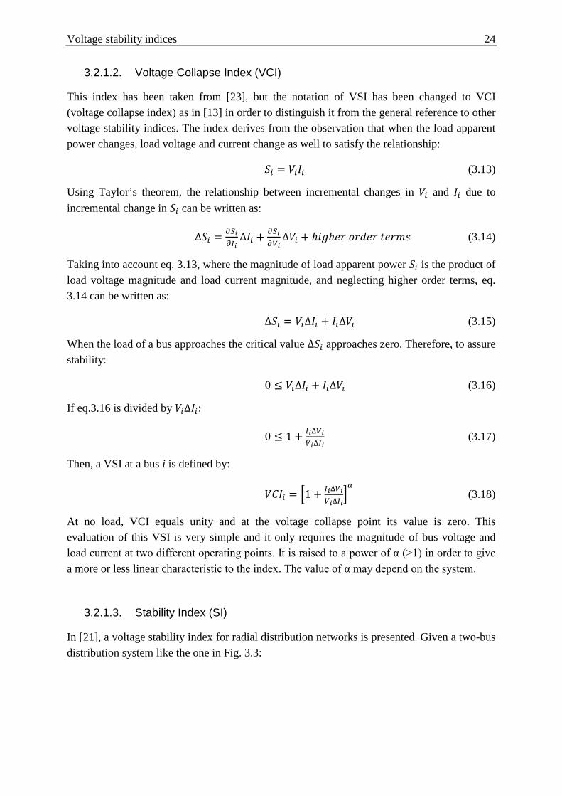
3.2.1.2. Voltage Collapse Index (VCI)
This index has been taken from [23], but the notation of VSI has been changed to VCI (voltage collapse index) as in [13] in order to distinguish it from the general reference to other voltage stability indices. The index derives from the observation that when the load apparent power changes, load voltage and current change as well to satisfy the relationship:
𝑆𝑖 = 𝑉𝑖𝐼𝑖 (3.13)
Using Taylor’s theorem, the relationship between incremental changes in 𝑉𝑖 and 𝐼𝑖 due to incremental change in 𝑆𝑖 can be written as:
∆𝑆𝑖 = 𝜕𝑆𝑖𝜕𝐼𝑖
∆𝐼𝑖 + 𝜕𝑆𝑖𝜕𝑉𝑖
∆𝑉𝑖 + ℎ𝑖𝑔ℎ𝑒𝑟 𝑜𝑟𝑑𝑒𝑟 𝑡𝑒𝑟𝑚𝑠 (3.14)
Taking into account eq. 3.13, where the magnitude of load apparent power 𝑆𝑖 is the product of load voltage magnitude and load current magnitude, and neglecting higher order terms, eq. 3.14 can be written as:
∆𝑆𝑖 = 𝑉𝑖∆𝐼𝑖 + 𝐼𝑖∆𝑉𝑖 (3.15)
When the load of a bus approaches the critical value ∆𝑆𝑖 approaches zero. Therefore, to assure stability:
0 ≤ 𝑉𝑖∆𝐼𝑖 + 𝐼𝑖∆𝑉𝑖 (3.16)
If eq.3.16 is divided by 𝑉𝑖∆𝐼𝑖:
0 ≤ 1 + 𝐼𝑖∆𝑉𝑖𝑉𝑖∆𝐼𝑖
(3.17)
Then, a VSI at a bus i is defined by:
𝑉𝐶𝐼𝑖 = 1 + 𝐼𝑖∆𝑉𝑖𝑉𝑖∆𝐼𝑖
𝛼
(3.18)
At no load, VCI equals unity and at the voltage collapse point its value is zero. This evaluation of this VSI is very simple and it only requires the magnitude of bus voltage and load current at two different operating points. It is raised to a power of α (>1) in order to give a more or less linear characteristic to the index. The value of α may depend on the system.
3.2.1.3. Stability Index (SI)
In [21], a voltage stability index for radial distribution networks is presented. Given a two-bus distribution system like the one in Fig. 3.3:
Voltage stability indices 25
Fig. 3.3 Two-bus system
Then, the a VSI is defined as,
SI(r) = 2Vs2Vr
2 − Vr4 − 2Vr
2(PR + QX) − |Z|2(P2 + Q2) (3.19)
After the load flow study, the voltages of all nodes and the branch currents are known, then P and Q can be calculated at the receiving end of each line and finally eq. 3.19 can be easily computed. It is considered that the node with the minimum value of the stability index is the most sensitive to voltage collapse.
This VSI has been developed from the mostly used quadratic equation to calculate the line sending end voltages in load flow analysis which can be written as:
Vr4 + 2Vr
2(PR + QX) − Vs2Vr
2 + (P2 + Q2)|Z|2 = 0 (3.20)
From eq. 3.20, line receiving end active and reactive power can be written as:
𝑃 = (− cos 𝜃𝑉𝑟2 ± 𝑐𝑜𝑠2𝜃𝑉𝑟
4 − 𝑉𝑟4 − |Z|2Q2 − 2Vr
2QX + Vs2Vr
2)/|Z| (3.21)
𝑄 = (− sin 𝜃𝑉𝑟2 ± 𝑠𝑖𝑛2𝜃𝑉𝑟
4 − 𝑉𝑟4 − |Z|2P2 − 2Vr
2PR + Vs2Vr
2)/|Z| (3.22)
The condition for the solution existence is therefore:
𝑐𝑜𝑠2𝜃𝑉𝑟4 − 𝑉𝑟
4 − |Z|2Q2 − 2Vr2QX + Vs
2Vr2 ≥ 0 (3.23)
𝑠𝑖𝑛2𝜃𝑉𝑟4 − 𝑉𝑟
4 − |Z|2P2 − 2Vr2PR + Vs
2Vr2 ≥ 0 (3.24)
The sum of both equations is then,
2Vs2Vr
2 − Vr4 − 2Vr
2(PR + QX) − |Z|2(P2 + Q2) ≥ 0 (3.25)
which is the VSI previously described.
3.2.2. Line stability indices
Most of line stability indices are formulated based on the power transmission concept in a single line. A single line in an interconnected network is illustrated in Fig. 3.4
𝑉𝑠 ∠0 𝑉𝑟∠θ
Z=R+jX P+jQ
Voltage stability indices 26
Fig. 3.4 Two bus system
Where,
𝑉𝑠 𝑎𝑛𝑑 𝑉𝑟 are the sending end and receiving end voltages, respectively.
𝛿𝑠 𝑎𝑛𝑑 𝛿𝑟 are the phase angle at the sending and receiving buses.
Z is the line impedance.
R is the line resistance.
X is the line reactance.
θ is the line impedance angle.
𝑄𝑟 is the reactive power at the receiving end.
𝑃𝑟 is the active power at the receiving end.
3.2.2.1. Lmn Index
This index proposed in [24] is based on the concept of power flow through a single line and adopting the technique of reducing a power system network into a single line.
From the power flow equations,
𝑆𝑟 = |𝑉𝑠||𝑉𝑟|𝑍
∠(𝜃 − 𝛿𝑠 + 𝛿𝑟) − |𝑉𝑟|2
𝑍∠𝜃 (3.26)
If this equation is separated in real and reactive power, then,
𝑃𝑟 = 𝑉𝑠𝑉𝑟𝑍
𝑐𝑜𝑠(𝜃 − 𝛿𝑠 + 𝛿𝑟) − 𝑉𝑟2
𝑍𝑐𝑜𝑠𝜃 (3.27)
𝑄𝑟 = 𝑉𝑠𝑉𝑟𝑍
𝑠𝑖𝑛(𝜃 − 𝛿𝑠 + 𝛿𝑟) − 𝑉𝑟2
𝑍𝑠𝑖𝑛𝜃 (3.28)
Defining 𝛿 = 𝛿𝑠 − 𝛿𝑟 and solving eq. for 𝑉𝑟, then,
𝑉𝑟 = 𝑉𝑠𝑠𝑖𝑜(𝜃−𝛿)±[𝑉𝑠𝑠𝑖𝑜(𝜃−𝛿)]2−4𝑍𝑄𝑟𝑠𝑖𝑜𝜃0.5
2𝑠𝑖𝑜𝜃 (3.29)
If we substitute Zsin𝜃 = 𝑋 and consider the condition that the value of the square root has to be positive,
Z=R+jX
𝑉𝑠∠𝛿𝑠 𝑉𝑟∠𝛿𝑟
𝑆𝑟 = 𝑃𝑟 + 𝑗𝑄𝑟
Voltage stability indices 27
[𝑉𝑠𝑠𝑖𝑛(𝜃 − 𝛿)]2 − 4𝑄𝑟𝑋 ≥ 0 (3.30)
Or otherwise,
𝐿𝑚𝑜 = 4𝑋𝑄𝑟[𝑉𝑠 sin(𝜃−𝛿)]2 ≤ 1 (3.31)
This VSI is used to find the stability index for each line connection between two bus bars in an interconnected network. As long as 𝐿𝑚𝑜 remains less than 1 the system is stable.
3.2.2.2. Line Voltage Stability Index (LVSI)
A similar index is proposed in [42], but from the viewpoint of the relationship between the lines reactive power and the bus voltage at the sending end. The index is defined as:
LVSI =4𝑟𝑃𝑟
[𝑉𝑠 cos(𝜃 − 𝛿)]2 ≤ 1
3.2.2.3. LQP Index
This index defined in [25] uses the same concept as in the previous index Lmn. Using the same notation, the proposed index is calculated as following:
𝐿𝑄𝑃 = 4 𝑋𝑉𝑖
2 𝑋𝑉𝑖
2 𝑃𝑖2 + 𝑄𝑗 (3.32)
3.2.2.4. Fast Voltage Stability Index (FVSI)
This index proposed by [26] stands for Fast Voltage Stability Index (FVSI) and it is also based on the concept of power flow through a single line. It is developed starting by taking the sending bus as the reference and using the general current equation:
𝐼 = 𝑉𝑠∠0−𝑉𝑟∠𝛿𝑅+𝑗𝑋
(3.33)
The roots for the receiving voltage can be written as:
𝑉𝑟 =𝑅
𝑋 sin 𝛿+cos 𝛿𝑉𝑠±𝑅𝑋 sin 𝛿+cos 𝛿𝑉𝑠
2−4(𝑋+𝑅2
𝑋 )𝑄𝑟
2 (3.34)
To obtain real roots for 𝑉𝑟, the discriminant has to be set greater than or equal to zero, then:
4𝑍2𝑄𝑟𝑋𝑉𝑠
2(𝑅𝑠𝑖𝑜𝛿+𝑋𝑐𝑐𝑠𝛿)2 ≤ 1 (3.35)
Since the angle difference is normally very small, the following simplification is done:
𝛿 ≈ 0 → 𝑠𝑖𝑛𝛿 = 0 & cos 𝛿 = 1 (3.36)
Voltage stability indices 28
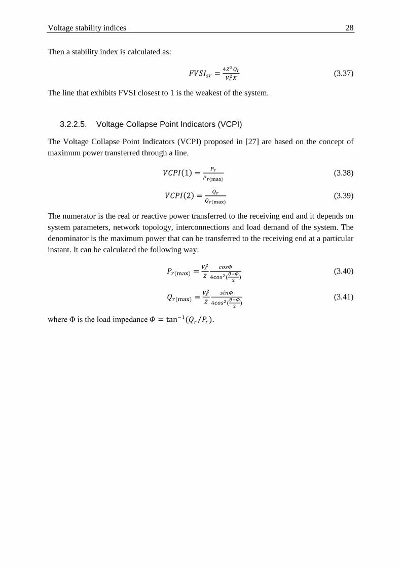
Then a stability index is calculated as:
𝐹𝑉𝑆𝐼𝑠𝑟 = 4𝑍2𝑄𝑟𝑉𝑠
2𝑋 (3.37)
The line that exhibits FVSI closest to 1 is the weakest of the system.
3.2.2.5. Voltage Collapse Point Indicators (VCPI)
The Voltage Collapse Point Indicators (VCPI) proposed in [27] are based on the concept of maximum power transferred through a line.
𝑉𝐶𝑃𝐼(1) = 𝑃𝑟𝑃𝑟(max)
(3.38)
𝑉𝐶𝑃𝐼(2) = 𝑄𝑟𝑄𝑟(max)
(3.39)
The numerator is the real or reactive power transferred to the receiving end and it depends on system parameters, network topology, interconnections and load demand of the system. The denominator is the maximum power that can be transferred to the receiving end at a particular instant. It can be calculated the following way:
𝑃𝑟(max) = 𝑉𝑠2
𝑍𝑐𝑐𝑠𝛷
4𝑐𝑐𝑠2(𝜃−𝛷2 )
(3.40)
𝑄𝑟(max) = 𝑉𝑠2
𝑍𝑠𝑖𝑜𝛷
4𝑐𝑐𝑠2(𝜃−𝛷2 )
(3.41)
where Φ is the load impedance 𝛷 = tan−1(𝑄𝑟 𝑃𝑟⁄ ).
Voltage stability indices 29
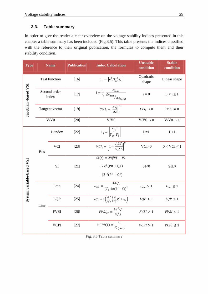
3.3. Table summary
In order to give the reader a clear overview on the voltage stability indices presented in this chapter a table summary has been included (Fig.3.5). This table presents the indices classified with the reference to their original publication, the formulas to compute them and their stability condition.
Type Name Publication Index Calculation Unstable condition
Stable condition
Jaco
bian
-bas
ed V
SI
Test function [16] 𝑡𝑐𝑐 = 𝑒𝑐𝑇𝐽𝐽𝑐𝑐
−1𝑒𝑐 Quadratic
shape Linear shape
Second order index [17] 𝑖 =
1𝑖0
𝜎max
𝑑𝜎max 𝑑𝜆𝑡𝑐𝑡𝑎𝑐
i = 0 0 < i ≤ 1
Tangent vector [19] 𝑇𝑉𝐼𝑖 = 𝑑𝑉𝑖
𝑑𝜆
−1
𝑇𝑉𝐼𝑖 → 0 𝑇𝑉𝐼𝑖 ≠ 0
V/V0 [20] V/V0 V/V0 → 0 V/V0 → 1
Syst
em v
aria
ble-
base
d V
SI
Bus
L index [22] Lj = 𝑆𝑗+
∗
𝑌𝑗𝑗+𝑉𝑗2 L=1 L<1
VCI [23] 𝑉𝐶𝐼𝑖 = 1 +𝐼𝑖∆𝑉𝑖
𝑉𝑖∆𝐼𝑖
𝛼
VCI=0 0 < VCI ≤ 1
SI [21]
SI(r) = 2Vs2Vr
2 − Vr4
−2Vr2(PR + QX)
−|Z|2(P2 + Q2)
SI<0 SI≥0
Line
Lmn [24] 𝐿𝑚𝑛 =4𝑋𝑄𝑟
[𝑉𝑠 sin(𝜃 − 𝛿)]2 𝐿𝑚𝑛 > 1 𝐿𝑚𝑛 ≤ 1
LQP [25] 𝐿𝑄𝑃 = 4 𝑋
𝑉𝑖2
𝑋𝑉𝑖
2 𝑃𝑖2 + 𝑄𝑗 𝐿𝑄𝑃 > 1 𝐿𝑄𝑃 ≤ 1
FVSI [26] 𝐹𝑉𝑆𝐼𝑠𝑟 =4𝑍2𝑄𝑟
𝑉𝑠2𝑋
𝐹𝑉𝑆𝐼 > 1 𝐹𝑉𝑆𝐼 ≤ 1
VCPI [27] 𝑉𝐶𝑃𝐼(1) =𝑃𝑟
𝑃𝑟(max) 𝑉𝐶𝑃𝐼 > 1 𝑉𝐶𝑃𝐼 ≤ 1
Fig. 3.5 Table summary
PMU-based voltage stability analysis 30
4. PMU-based voltage stability analysis
The development of phasor measurement technology together with other advances in computational facilities, networking infrastructure and communications has opened new perspectives for wide-area monitoring and control [29]. This fact has enabled the development of new methods for assessing voltage stability. This chapter will firstly present phasor measurements units and its characteristics and secondly, will deal with the different methods that have evolved using this technology.
4.1. Synchrophasors and phasor measurement units
An AC waveform can be mathematically represented by the following equation:
𝑥(𝑡) = 𝑋𝑚𝑐𝑜𝑠(𝜔𝑡 + 𝜑) (4.1)
where:
𝑋𝑚 is the magnitude of the sinusoidal waveform
𝜔 is the angular frequency given by 𝜔 = 2𝜋𝑓 and f being the frequency in Hz
𝜑 is the angular starting point for the waveform.
The representation of power system sinusoidal signals is commonly done in phasor notation. The waveform is then represented as 𝑋 = 𝑋𝑚 ∠𝜑. The phasor representation of a sinusoid is independent of its frequency and the phase angle φ of the phasor is determined by the starting time (t= 0) of the sinusoid.
Fig. 4.1 Phasor representation of waveforms
PMU-based voltage stability analysis 31
The standard [28] defines the synchronized phasors (or synchrophasor) as a complex number representation of the fundamental frequency component of either a voltage or a current, with a time label defining the time instant for which the phasor measurement is performed. The synchrophasor representation X of a signal x(t) is the complex value given by:
𝑋 = 𝑋𝑟 + 𝑗𝑋𝑖 = 𝑋𝑚
√2 𝑒𝑗𝜑 = 𝑋𝑚
√2 (𝑐𝑜𝑠 𝜑 + 𝑗 𝑠𝑖𝑛 𝜑) (4.2)
where 𝑋𝑚
√2 is the RMS (Root Mean Square) value of the signal x(t) and φ is its instantaneous
phase angle relative to a cosine function at nominal system frequency synchronized to universal time coordinated (UTC).
Note that the synchrophasor standard defines the phasor refered to the RMS value. Therefore, it should be taken into account that √2 should be multiplied to the synchrophasor value when computing the actual phasor magnitude.
Phasor Measurement Units (PMUs) units are devices that provide real time measurement of positive sequence voltages and currents at power system substations. Typically the measurement windows are one cycle of the fundamental frequency. Through the use of integral GPS (Global Positioning System) satellite receiver-clocks, PMUs sample synchronously at selected locations throughout the power system. Data from substations are collected at a suitable site, and by aligning the time stamps of the measurements a coherent picture of the state of the power system is created [46]. Therefore a wide implementation of PMU offers new opportunities in power system monitoring, protection, analysis and control.
The commercialization of PMU together with high-speed communications networks makes it possible to build wide area monitoring systems (WAMSs), which takes snapshots of the power system variables within one second and provides new perspectives for early detection and prevention of voltage instability. As stated in [29], PMU-based voltage instability monitoring can be classified in two broad categories: methods based on local measurements and methods based on the observability of the whole region. The first, need few or no information exchange between the monitoring locations, while the second one requires time-synchronized measurements. The following sections will provide information on both types and will expose different methods of each type.
4.2. Methods based on local measurements
PMU-methods based on local measurements, can be implemented in a distributed manner and require few or no information exchange between monitoring locations. These methods accommodate the time skew of SCADA data and no time synchronization is needed [29]. Most of these methods rely on the Thevenin impedance matching condition or its extensions and are based on the assumption that voltage instability is closely related to maximum loadability of a transmission network. Figure 4.1 shows a load bus and the rest of the system treated as a Thevenin equivalent.
PMU-based voltage stability analysis 32
Fig. 4.1 Load bus Thevenin equivalent [43]
The receiving and sending currents for the power system as shown in Fig. 4.1 are
𝑆𝑘𝑈𝑘
= 𝐼𝑘∗ = (𝐸−𝑈𝑘
𝑍𝑇ℎ)∗ (4.3)
Equation (4.2) can be written as follows:
(𝐸 − 𝑈𝑘)∗𝑈𝑘 − 𝑆𝑘𝑍𝑇ℎ∗ = 0 (4.4)
For a given power 𝑆𝑘, the phasor equation (4.3) permits at most two voltage solutions 𝑈𝑘. Maximum power transfer occurs when these solutions become equal:
(𝐸 − 𝑈𝑘)∗ = 𝑈𝑘 (4.5)
Equation (4.4) leads to the following result:
𝑍𝑘 = 𝑍𝑇ℎ (4.6)
Therefore, when the magnitude of the load impedance becomes equal to the magnitude of the Thevenin’s impedance, the system reaches the maximum deliverable power. The impedance 𝑍𝑘 is the ratio between the voltage 𝑉 and current 𝐼 phasors measured at the bus through PMU. When the loading is normal, 𝑍𝑘 ≫ 𝑍𝑇ℎ and are equal at the point of collapse. Therefore, calculating the distance between 𝑍𝑘 and 𝑍𝑇ℎ can be used as a voltage stability index to assess the closeness to voltage instability. This section will present both, on one hand, different methods to calculate the Thevenin equivalent and on the other hand, indices or criterions used once the equivalent is calculated to assess proximity to instability. The first three sections will deal with calculating the Thevenin equivalent, which can be done by least square method, though the use of both ends of a transmission corridor or using an approximation. The following sections will present voltage stability indices or margins that can be used once the Thevenin is computed.
4.2.1. Thevenin equivalent using least-square method
In [33], the measurements collected from one load bus are used to obtain the Thevenin equivalent of the system seen from the bus, as well as the impedance of the load. Therefore, it must use successive measurements and the parameters of the Thevenin are estimated using a least-square method once a couple of sets of measurements are available.
𝑍𝑡ℎ 𝑈𝑘
𝐸𝑡ℎ
𝑆𝑘 , 𝐼𝑘, 𝑍𝑘
PMU-based voltage stability analysis 33
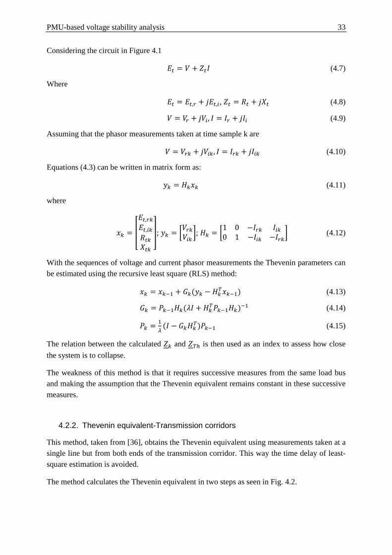
Considering the circuit in Figure 4.1
𝐸𝑡 = 𝑉 + 𝑍𝑡𝐼 (4.7)
Where
𝐸𝑡 = 𝐸𝑡,𝑟 + 𝑗𝐸𝑡,𝑖, 𝑍𝑡 = 𝑅𝑡 + 𝑗𝑋𝑡 (4.8)
𝑉 = 𝑉𝑟 + 𝑗𝑉𝑖, 𝐼 = 𝐼𝑟 + 𝑗𝐼𝑖 (4.9)
Assuming that the phasor measurements taken at time sample k are
𝑉 = 𝑉𝑟𝑘 + 𝑗𝑉𝑖𝑘, 𝐼 = 𝐼𝑟𝑘 + 𝑗𝐼𝑖𝑘 (4.10)
Equations (4.3) can be written in matrix form as:
𝑦𝑘 = 𝐻𝑘𝑥𝑘 (4.11)
where
𝑥𝑘 =
𝐸𝑡,𝑟𝑘𝐸𝑡,𝑖𝑘𝑅𝑡𝑘𝑋𝑡𝑘
; 𝑦𝑘 = 𝑉𝑟𝑘𝑉𝑖𝑘
; 𝐻𝑘 = 1 0 −𝐼𝑟𝑘0 1 −𝐼𝑖𝑘
𝐼𝑖𝑘−𝐼𝑟𝑘
(4.12)
With the sequences of voltage and current phasor measurements the Thevenin parameters can be estimated using the recursive least square (RLS) method:
𝑥𝑘 = 𝑥𝑘−1 + 𝐺𝑘(𝑦𝑘 − 𝐻𝑘𝑇𝑥𝑘−1) (4.13)
𝐺𝑘 = 𝑃𝑘−1𝐻𝑘(𝜆𝐼 + 𝐻𝑘𝑇𝑃𝑘−1𝐻𝑘)−1 (4.14)
𝑃𝑘 = 1𝜆
(𝐼 − 𝐺𝑘𝐻𝑘𝑇)𝑃𝑘−1 (4.15)
The relation between the calculated 𝑍𝑘 and 𝑍𝑇ℎ is then used as an index to assess how close the system is to collapse.
The weakness of this method is that it requires successive measures from the same load bus and making the assumption that the Thevenin equivalent remains constant in these successive measures.
4.2.2. Thevenin equivalent-Transmission corridors
This method, taken from [36], obtains the Thevenin equivalent using measurements taken at a single line but from both ends of the transmission corridor. This way the time delay of least-square estimation is avoided.
The method calculates the Thevenin equivalent in two steps as seen in Fig. 4.2.
PMU-based voltage stability analysis 34
Fig. 4.2 First step calculation
First, the parameters of a T-equivalent of the transmission corridor can be determined through a direct calculation from the PMU measurements 𝑣1, 2, 𝚤1 ,𝚤2:
𝑇 = 2 𝑣1−𝑣2𝚤1−𝚤2
(4.16)
𝑠ℎ = 𝑣1𝚤2−𝑣2𝚤1𝚤22−𝚤12 (4.17)
𝐿 = 𝑣2−𝚤2
(4.18)
𝑔is assumed to be known since it typically comprises the step-up transformers and short transmission line to the beginning of the transmission corridor and 𝐸𝑔is calculated as:
𝐸𝑔 = 1 + 𝑔𝚤1 (4.19)
Then, the second step calculates the Thevenin equivalent shown in Fig. 4.3.
Fig. 4.3 : Second step calculation
The equations used to compute the voltage and impedance equivalent are the following:
𝑡ℎ = 𝑍𝑇2
+ 11
𝑍𝑠ℎ+ 1
𝑍𝑇2 +𝑍𝑔
(4.20)
𝐸𝑡ℎ = 𝑣2𝑍𝑡ℎ+𝑍𝐿
𝑍𝐿 (4.21)
Based on this Thevenin equivalent, stability analysis can then be performed. In terms of load impedance in percentage, stability margin can be expressed as:
𝑍𝑡ℎ 𝑖2
𝑣2 𝑍𝐿
𝐸𝑡ℎ
𝑍𝑔
𝑣1
𝑖1
𝑍𝑇/2
𝑍𝑇/2
𝑠ℎ
𝑖2
𝑣2
𝑍𝐿
𝐸𝑔
PMU-based voltage stability analysis 35
𝑀𝐴𝑅𝐺𝐼𝑁𝑍 = 100(1 − 𝑘𝑐𝑟𝑖𝑡) (4.22)
𝑘𝑐𝑟𝑖𝑡 = 𝑍𝑡ℎ
𝑍𝐿 (4.23)
4.2.3. Thevenin equivalent-Approximate approach
The buses in an interconnected power system can generally be classified into three categories: generator bus, load bus and tie bus (without generators and loads connecting to it). A generator bus will become a load bus if its power capacity limit is reached. Since the injection currents to the tie buses are zero, the injection currents into the three types of buses can be generally expressed as [45],
−𝑖𝐿
0𝑖𝐺
= 𝑌𝐿𝐿 𝑌𝐿𝑇 𝑌𝐿𝐺𝑌𝑇𝐿 𝑌𝑇𝑇 𝑌𝑇𝐺𝑌𝐺𝐿 𝑌𝐺𝑇 𝑌𝐺𝐺
𝑣𝐿𝑣𝑇𝑣𝐺
(4.24)
where the Y matrix is known as the system admittance matrix, V and I stand for the voltage and current vectors, and the subscript L, T and G represent load bus, tie bus and generator bus, respectively.
According to (4.23), the load bus voltages can be expressed as
where 𝑍𝐿𝐿𝑖𝑖 denotes the ith diagonal element of 𝑍𝐿𝐿, 𝑍𝐿𝐿𝑗𝑖 is the i–j element of 𝑍𝐿𝐿, 𝐸𝑐𝑐𝑒𝑜,𝑖 is the open-circuit voltage of load i, n is the number of load buses, and 𝑉𝐿𝑖 and I𝐿𝑖 are the voltage and current of load i, respectively.
In (4.27), 𝑉𝐿𝑖 consists of three terms: the open-circuit voltage, the voltage related to the self-impedance 𝑍𝐿𝐿𝑖𝑖 and the coupling voltage related to the mutual-impedance 𝑍𝐿𝐿𝑗𝑖, which represents the impact of other loads on load i [45].
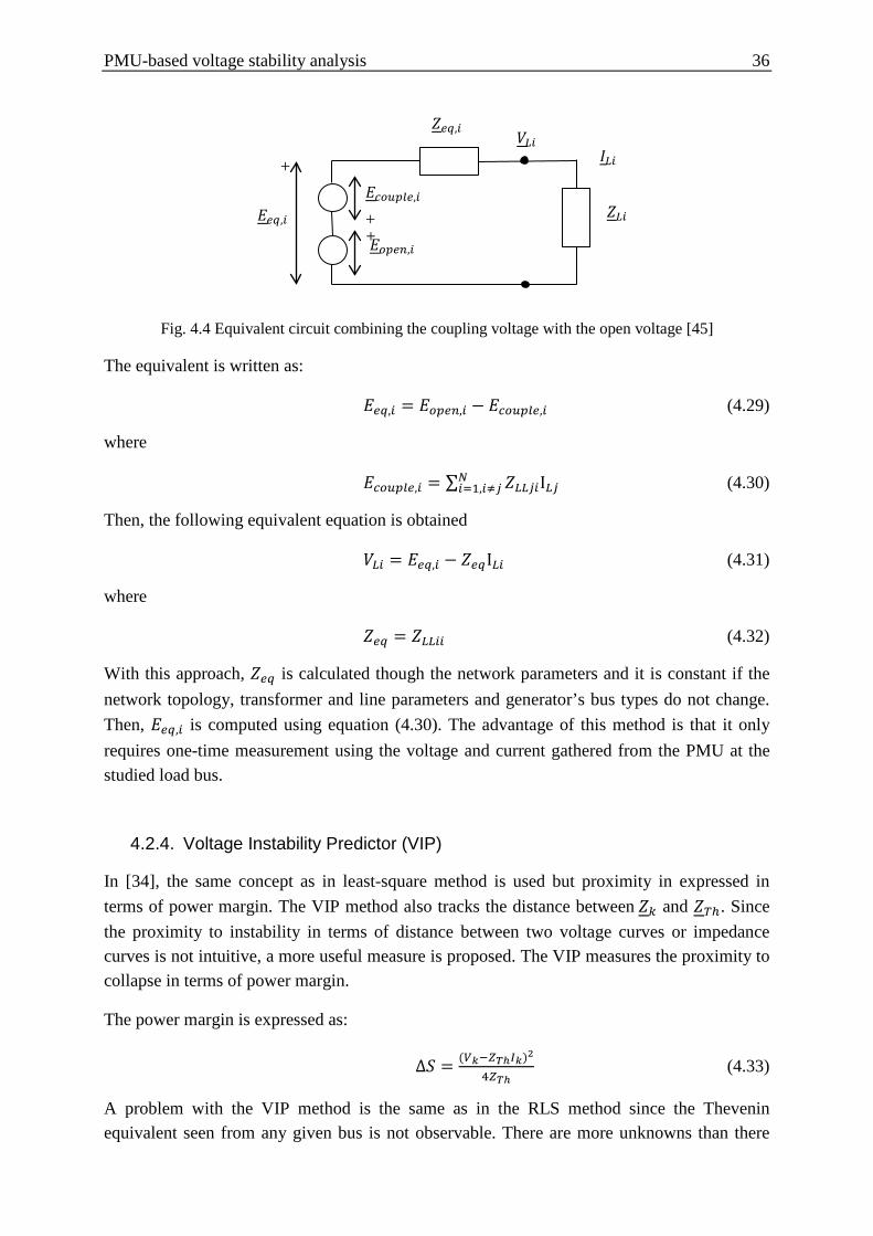
In [45] an approximate approach is presented to combine the coupling term with the open-circuit voltage to form the equivalent voltage, which is shown Fig. 4.4.
PMU-based voltage stability analysis 36
Fig. 4.4 Equivalent circuit combining the coupling voltage with the open voltage [45]
The equivalent is written as:
𝐸𝑒𝑒,𝑖 = 𝐸𝑐𝑐𝑒𝑜,𝑖 − 𝐸𝑐𝑐𝑐𝑐𝑐𝑒,𝑖 (4.29)
where
𝐸𝑐𝑐𝑐𝑐𝑐𝑒,𝑖 = ∑ 𝑍𝐿𝐿𝑗𝑖I𝐿𝑗𝑁𝑖=1,𝑖≠𝑗 (4.30)
Then, the following equivalent equation is obtained
𝑉𝐿𝑖 = 𝐸𝑒𝑒,𝑖 − 𝑍𝑒𝑒I𝐿𝑖 (4.31)
where
𝑍𝑒𝑒 = 𝑍𝐿𝐿𝑖𝑖 (4.32)
With this approach, 𝑍𝑒𝑒 is calculated though the network parameters and it is constant if the network topology, transformer and line parameters and generator’s bus types do not change. Then, 𝐸𝑒𝑒,𝑖 is computed using equation (4.30). The advantage of this method is that it only requires one-time measurement using the voltage and current gathered from the PMU at the studied load bus.
4.2.4. Voltage Instability Predictor (VIP)
In [34], the same concept as in least-square method is used but proximity in expressed in terms of power margin. The VIP method also tracks the distance between 𝑍𝑘 and 𝑍𝑇ℎ. Since the proximity to instability in terms of distance between two voltage curves or impedance curves is not intuitive, a more useful measure is proposed. The VIP measures the proximity to collapse in terms of power margin.
The power margin is expressed as:
∆𝑆 = (𝑉𝑘−𝑍𝑇ℎ𝐼𝑘)2
4𝑍𝑇ℎ (4.33)
A problem with the VIP method is the same as in the RLS method since the Thevenin equivalent seen from any given bus is not observable. There are more unknowns than there
𝑍𝑒𝑒,𝑖
𝐼𝐿𝑖 𝑉𝐿𝑖
𝑍𝐿𝑖
𝐸𝑒𝑒,𝑖
𝐸𝑐𝑐𝑐𝑐𝑐𝑒,𝑖
𝐸𝑐𝑐𝑒𝑜,𝑖
+
++
PMU-based voltage stability analysis 37
are equations, which mean that there is an infinite set of Thevenin equivalents that could all produce the same results as the one that is observed. This is solved by taking measurements at two or more different times, and treating the Thevenin equivalent as a constant.
4.2.5. Voltage Stability Load Bus Index (VSLBI)
In [37], the Thevenin equivalent is calculated using the RLS method explained in section 4.2.1 and then a voltage stability load bus index (VSLBI) is defined as:
𝑉𝑆𝐿𝐵𝐼𝑘 = |𝑉𝑖(𝑘)||∆𝑉𝑖(𝑘)| (4.34)
Where 𝑉𝑖(𝑘) is the amplitude of the load bus voltage i at time step k and ∆𝑉𝑖(𝑘) = 𝑍𝑇ℎ,𝑘𝐼𝑘 is the voltage drop across the Thevenin equivalent impedance 𝑍𝑇ℎ. If the value approaches 1, the system may be close to instability. This index can be calculated in each load bus and then a system voltage stability index can be defined as the smallest of all VSLBI:
𝑉𝑆𝐼 = min𝑖∈𝛼𝑃𝑄 𝑉𝑆𝐿𝐵𝐼𝑖,𝑘 (4.35)
4.2.6. S Difference Criterion (SDC)
The S difference criterion (SDC) method proposed in [38] and [39] uses consecutive measurements of the apparent power S in a line’s relay points. It is based in the fact that in the vicinity of voltage instability an increase in the apparent power flow at the sending end of the line no longer yields an increase in the received power. Therefore, at the voltage instability point, ∆𝑆 = 0.
The apparent power supplied at the receiving end can be written as:
𝑆,𝑘 = 𝑈𝑗,𝑘𝐼𝑖,𝑘∗ (4.36)
An increase in the apparent power loading in the time interval between 𝑡𝑘 and 𝑡𝑘+1 = 𝑡𝑘 + ∆𝑡 is:
The term +∆𝑈𝑗,𝑘+1∆𝐼𝑖,𝑘+1∗can be neglected, since it represents a very small value.
Then,
∆𝑆,𝑘+1 = ∆𝑈𝑗,𝑘+1𝐼𝑖,𝑘∗ + 𝑈𝑗,𝑘∆𝐼𝑖,𝑘+1
∗ (4.38)
Since it is known that ∆𝑆,𝑘+1 = 0 at the point of collapse, an index can be defined dividing
Equation (4.23) by 𝑈𝑗,𝑘∆𝐼𝑖,𝑘+1∗:
PMU-based voltage stability analysis 38
𝑆𝐶𝐷 = 1 + ∆𝑈𝑗,𝑘+1𝐼𝑖,𝑘∗
𝑈𝑗,𝑘∆𝐼𝑖,𝑘+1∗ = 1 + 𝑎𝑒𝑗𝜑 (4.39)
4.3. Methods based on the observability of the whole region
On the other hand, PMU-methods based on the observability of the whole region require time-synchronized measurements and offer the potential advantages of wide-area monitoring [29].
4.3.1. Sensitivities
A PMU-method based on the observability of the whole region is presented in [29]-[31]. The work focuses on detecting the onset of voltage instability triggered by a large disturbance. The method fits a set of algebraic equations to the sampled states, computed from PMUs measurements and performs an efficient sensitivity computation, which tracks the eigenvalue movement around a maximum load power point.
As seen in Section 2.3.1, voltage stability can be determined by computing the eigenvalues and eigenvectors of the reduced Jacobian matrix. Given an eigenvalue 𝜆𝑖 of the ith mode of the Q-V response, if it is greater than 0, then the modal voltage and modal reactive power are along the same direction which yields to a voltage stable system. If 𝜆𝑖 < 0, the modal voltage and modal reactive power are along opposite directions which indicates an unstable system. Therefore, the change of sign of the eigenvalue can indicate the pass from a stable to an unstable point. This fact is used in [28] to assess voltage stability.
It is stated in [29]-[31], that in order to detect this change in sign, there is no need to explicitly compute the eigenvalues. Instead, sensitivities involving the inverse Jacobian can be used.
Given the static model of a power system:
0 = 𝑔(𝑥, 𝑦) (4.40)
where x represents the state vector of the system and y, the algebraic variables such as the active and reactive power consumed by the loads.
The sensitivities of the total reactive power generation to individual load reactive powers can be obtained using the following formula:
𝑆𝑄𝑔𝑒 = −𝑔𝑒𝑇(𝑔𝑥
𝑇)−1∇𝑥𝑄𝑔 (4.41)
Where, ∇𝑥𝑄𝑔denotes the gradient of 𝑄𝑔 with respect to x, 𝑔𝑒 is the Jacobian of g with respect to q and the load reactive powers are grouped into 𝑞 = [𝑄1 … 𝑄𝑁]𝑇.
Computing 𝑆𝑄𝑔𝑒 requires solving one linear system with 𝑔𝑥𝑇as a matrix of coefficients and
∇𝑥𝑄𝑔 as independent term.
PMU-based voltage stability analysis 39
4.3.2. Sum of the absolute values Index
The new method developed in [40] relies on measurements taken at current time and it is based on the fact that the amplitude of the complex voltage drop on the Thevenin’s impedance is equal to the amplitude of the voltage at the node at the point of maximum loadability, the nose of the PV curve. The assumption made is the generator nearest to a load can give information comparable with the Thevenin’s voltage.
The method defines the distance to a generator as the sum of the absolute values of the complex voltage drop for each line along the shortest path from a node to the generator. Nearest generator is the one this defined distance is minimum. Only generators that are in PV mode, controlling the active power and voltage at its output, should be considered for this calculation.
The voltage stability index is defined as:
𝑉𝑆𝐼𝑘 = 𝑉𝑘∆𝑉𝑘
(4.42)
Where 𝑉𝑘 is the voltage at node k and ∆𝑉𝑘 is the distance to the nearest generator as described in the paper. This distance approximates the voltage drop across the Thevenin’s impedance.
The minimum value of VSI represents the weakest bus of the system. If no assumption were made, it would be one at the maximum loadability point, therefore, a margin should be given, and the real maximum loadability point value will be greater than one.
Weakness of the method is also presented in the paper. Firstly, by using a global index, the location of the problem is not visible and secondly, a bad bus index that does not evolve taken as the global index could hide bad evolutions elsewhere.
4.3.3. Voltage Collapse Proximity Indicator (VCPI)
The technique described in [32] uses the voltage magnitude and voltage angle information at buses provided by PMUs, but also the network admittance matrix to predict proximity to voltage collapse.
The proposed index at bus k is calculated as:
𝑉𝐶𝑃𝐼𝑘 = 1 −∑ 𝑉𝑚
′𝑁𝑚=1𝑚≠𝑘
𝑉𝑘 (4.43)
Where:
𝑉𝑚′ = 𝑌𝑘𝑚
∑ 𝑌𝑘𝑗𝑁𝑗=1𝑗≠𝑘
𝑉𝑚 (4.44)
𝑉𝑘 is the voltage phasor at bus k
PMU-based voltage stability analysis 40
𝑌𝑘𝑚 is the admittance between buses k and m
The index varies from 0 to 1, being 1 if the voltage at the bus has collapsed.
4.3.4. Margin Voltage Stability Index (MVSI)
Another method based also on time-synchronized phasor measurements and network parameters is proposed in [10].
The index is based on the maximum transferable power through a transmission line and is expressed as:
𝑀𝑉𝑆𝐼 = min (𝑃𝑚𝑎𝑟𝑔𝑖𝑛
𝑃𝑚𝑎𝑥, 𝑄𝑚𝑎𝑟𝑔𝑖𝑛
𝑄𝑚𝑎𝑥, 𝑆𝑚𝑎𝑟𝑔𝑖𝑛
𝑆𝑚𝑎𝑥) (4.45)
where
𝑃𝑚𝑎𝑟𝑔𝑖𝑜 = 𝑃𝑚𝑎𝑥 − 𝑃 (4.46)
𝑄𝑚𝑎𝑟𝑔𝑖𝑜 = 𝑄𝑚𝑎𝑥 − 𝑄 (4.47)
𝑆𝑚𝑎𝑟𝑔𝑖𝑜 = 𝑆𝑚𝑎𝑥 − 𝑆 (4.48)
and
𝑃𝑚𝑎𝑥 = 𝑉𝑠4
4𝑋2 − 𝑄 𝑉𝑠2
𝑋 (4.49)
𝑄𝑚𝑎𝑥 = 𝑉𝑠4
4𝑋− 𝑃2𝑋
𝑉𝑠2 (4.50)
𝑆𝑚𝑎𝑥 = (1−𝑠𝑖𝑜𝜃)𝑉𝑠2
2(𝑐𝑐𝑠𝜃)2𝑋 (4.51)
In larger interconnected power systems the equivalent source voltage and equivalent impedance has to be calculated in each bus in order to calculate eq. (), () and (). The system admittance matrix can be calculated as:
𝑖𝐿𝑖𝑇𝑖𝐺
= 𝑌𝐿𝐿 𝑌𝐿𝑇 𝑌𝐿𝐺𝑌𝑇𝐿 𝑌𝑇𝑇 𝑌𝑇𝐺𝑌𝐺𝐿 𝑌𝐺𝑇 𝑌𝐺𝐺
𝑣𝐿𝑣𝑇𝑣𝐺
(4.52)
𝑣𝐿 = 𝑍𝐿𝐿𝑖𝐿 + 𝑍𝐿𝑇𝑖𝑇 + 𝐻𝐿𝐺𝑣𝐺 (4.53)
Where,
𝑍𝐿𝐿 = (𝑌𝐿𝐿 − 𝑌𝐿𝑇𝑌𝑇𝑇−1𝑌𝑇𝐿)−1 (4.54)
𝑍𝐿𝑇 = −𝑍𝐿𝐿𝑌𝐿𝑇𝑌𝑇𝑇−1 (4.55)
𝐻𝐿𝐺 = 𝑍𝐿𝐿(𝑌𝐿𝑇𝑌𝑇𝑇−1𝑌𝑇𝐺 − 𝑌𝐿𝐺) (4.56)
PMU-based voltage stability analysis 41
Then for a given bus j, the equivalent voltage source and line impedance can be calculated with the following equations:
𝑣𝑒𝑒𝑗 = ∑ 𝐻𝐿𝐺𝑗𝑘𝑣𝐺𝑘 + ∑ 𝑍𝐿𝐿𝑗𝑖 −𝑆𝐿𝑖𝑣𝐿𝑖
∗
𝑁𝑖=1,𝑖≠𝑗
𝑀𝑘=1 (4.57)
𝑍𝑒𝑒𝑗 = 𝑍𝐿𝐿𝑗𝑗 (4.58)
The load bus with the lowest MVSI has the smallest load margin and, therefore, is the closest to voltage collapse.
PMU-based voltage stability analysis 42
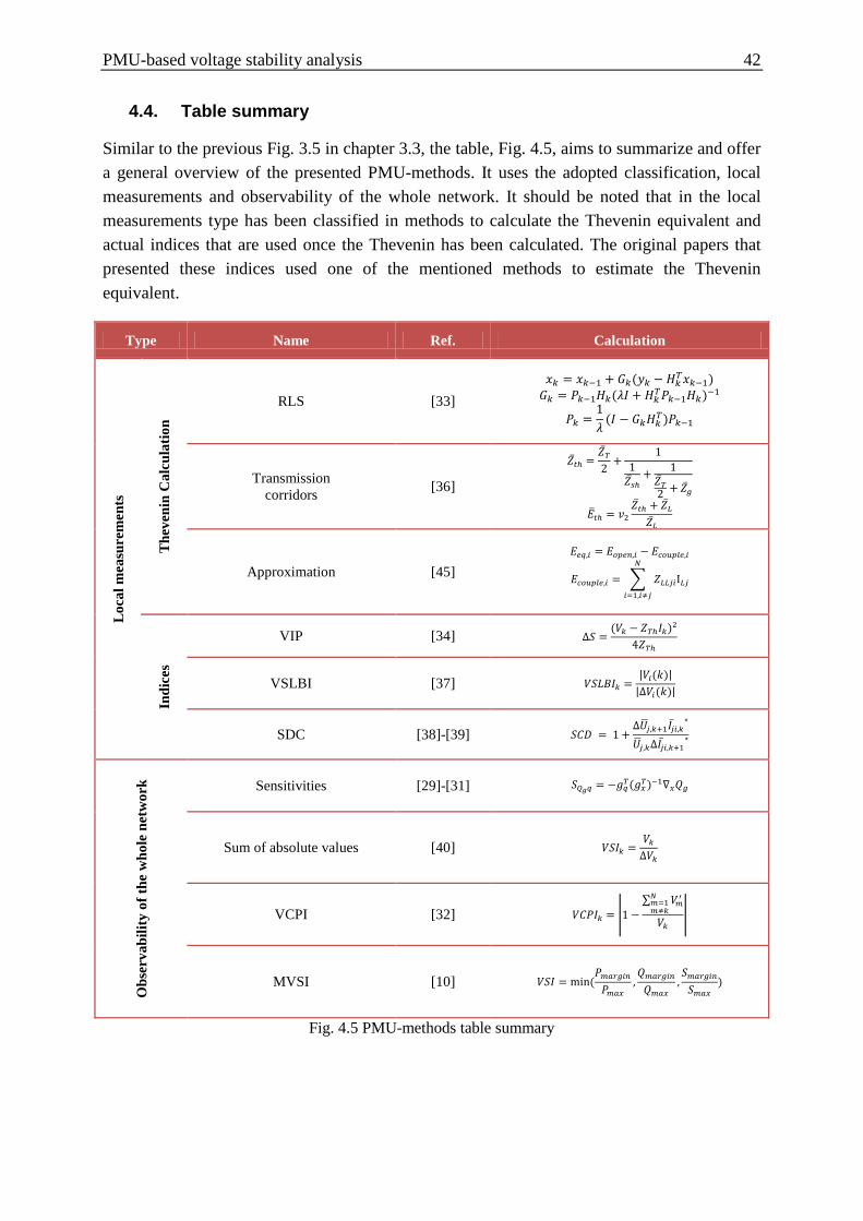
4.4. Table summary
Similar to the previous Fig. 3.5 in chapter 3.3, the table, Fig. 4.5, aims to summarize and offer a general overview of the presented PMU-methods. It uses the adopted classification, local measurements and observability of the whole network. It should be noted that in the local measurements type has been classified in methods to calculate the Thevenin equivalent and actual indices that are used once the Thevenin has been calculated. The original papers that presented these indices used one of the mentioned methods to estimate the Thevenin equivalent.
Type Name Ref. Calculation
Loc
al m
easu
rem
ents
The
veni
n C
alcu
latio
n
RLS [33] 𝑥𝑘 = 𝑥𝑘−1 + 𝐺𝑘(𝑦𝑘 − 𝐻𝑘
𝑇𝑥𝑘−1) 𝐺𝑘 = 𝑃𝑘−1𝐻𝑘(𝜆𝐼 + 𝐻𝑘
𝑇𝑃𝑘−1𝐻𝑘)−1
𝑃𝑘 =1𝜆 (𝐼 − 𝐺𝑘𝐻𝑘
𝑇)𝑃𝑘−1
Transmission corridors [36]
𝑡ℎ =𝑇
2+
11
𝑠ℎ+ 1
𝑇2 + 𝑔
𝐸𝑡ℎ = 𝑣2𝑡ℎ + 𝐿
𝐿
Approximation [45] 𝐸𝑒𝑒,𝑖 = 𝐸𝑐𝑐𝑒𝑜,𝑖 − 𝐸𝑐𝑐𝑐𝑐𝑐𝑒,𝑖
𝐸𝑐𝑐𝑐𝑐𝑐𝑒,𝑖 = 𝑍𝐿𝐿𝑗𝑖I𝐿𝑗
𝑁
𝑖=1,𝑖≠𝑗
Indi
ces
VIP [34] ∆𝑆 =(𝑉𝑘 − 𝑍𝑇ℎ𝐼𝑘)2
4𝑍𝑇ℎ
VSLBI [37] 𝑉𝑆𝐿𝐵𝐼𝑘 =|𝑉𝑖(𝑘)|
|∆𝑉𝑖(𝑘)|
SDC [38]-[39] 𝑆𝐶𝐷 = 1 +∆𝑈𝑗,𝑘+1𝐼𝑖,𝑘
∗
𝑈𝑗,𝑘∆𝐼𝑖,𝑘+1∗
Obs
erva
bilit
y of
the
who
le n
etw
ork Sensitivities [29]-[31] 𝑆𝑄𝑔𝑒 = −𝑔𝑒
𝑇(𝑔𝑥𝑇)−1∇𝑥𝑄𝑔
Sum of absolute values [40] 𝑉𝑆𝐼𝑘 =𝑉𝑘
∆𝑉𝑘
VCPI [32] 𝑉𝐶𝑃𝐼𝑘 = 1 −∑ 𝑉𝑚
′𝑁𝑚=1𝑚≠𝑘
𝑉𝑘
MVSI [10] 𝑉𝑆𝐼 = min (𝑃𝑚𝑎𝑟𝑔𝑖𝑜
𝑃𝑚𝑎𝑥,𝑄𝑚𝑎𝑟𝑔𝑖𝑜
𝑄𝑚𝑎𝑥,𝑆𝑚𝑎𝑟𝑔𝑖𝑜
𝑆𝑚𝑎𝑥)
Fig. 4.5 PMU-methods table summary
Stability Indices and methods comparison 43
5. Stability Indices and methods comparison
In the previous chapters, different indices and methods to assess voltage stability were presented. Since there has been a large amount of information given, this chapter aims to provide a summary of the indices and methods and present their main characteristics and difference. The three main types of indices were classified in Jacobian matrix-based, System parameters-based and PMU methods. From the system parameters, two subtypes were presented, line and bus indices; and the PMU methods are classified in two subtypes, local measurements and observability.
Jacobian matrix based VSIs can calculate the voltage collapse point or maximum loadability limit and determine the voltage stability margin, for that, the computation time is high; hence, they are not suitable for online assessment. They also present a high nonlinear profile near the voltage collapse point and they do not offer information on weak area or buses of the system, just a general view of the whole system. Therefore, they do not provide enough information to know where in the system there is a problem, and are difficult to use for control purposes.
On the other hand, system variables based VSIs, which use the elements of the admittance matrix and some system variables such as bus voltages or power flow through lines, require less computation and, therefore, are adequate for online monitoring. The disadvantage of these indices is that they cannot accurately estimate the margin, so they can just present critical lines and buses. By ranking the critical lines and buses, decisions on where to place shunt FACTS controllers, as done in [48], can be made. Some studies on how uncertainty affects line indices are pursued in [49], but conclude that more tests should be done in order to draw a general conclusion.
As stated in [29], PMU-based voltage instability monitoring can be classified in two broad categories: methods based on local measurements and methods based on the observability of the whole region. PMU-methods based on local measurements, can be implemented in a distributed manner and require few or no information exchange between monitoring locations. These methods accommodate the time skew of SCADA data and no time synchronization is needed [29]. Most of these methods rely on the Thevenin impedance matching condition or its extensions and are based on the assumption that voltage instability is closely related to maximum loadability of a transmission network. Three methods to compute the Thevenin equivalent are presented: RLS, Transmission corridor method and Approximation method. Once the Thevenin has been computed, there are several indices that can provide information on voltage stability; VSLBI and SLD, among others.
On the other hand, PMU-methods based on the observability of the whole region require time-synchronized measurements and offer the potential advantages of wide-area monitoring [29]. Therefore, the measurements require to be processed in a centralized manner.
Stability Indices and methods comparison 44
Type Index Characteristics Ja
cobi
an
mat
rix-
base
d Test function
Compute the whole network. Centralized measurements. High computational costs.
Non-linearity near voltage collapse. Difficult to use for control purposes.
Second order
Tangent vector
V/V0
Syst
em
vari
able
s. B
us
indi
ces.
L index
Easy to compute. Small computational costs.
Better results in transmission-radial networks than in interconnected networks.
VCI
SI
Syst
em v
aria
bles
. L
ine
indi
ces.
Lmn
Easy to compute. Small computational costs. Good for control purposes:
Identifies the weakest line in the network. FACTS placement. Distributed measurements.
LVSI
LQP
FVSI
VCPI
PMU
- L
ocal
m
easu
rem
ent
s
VIP
Distributed measurements and processing. Usable for control purposes. VSLBI
SDC
PMU
-Obs
erva
bilit
y Sensitivities
Centralized measurements and processing. Sum of absolute
value VCPI
Margin VSI
Fig. 5.1 Index classification and comparison
Implementation of Voltage Stability Indices and test networks 45
6. Implementation of Voltage Stability Indices and test networks
The software used to simulate the networks is RSCAD, which is the Graphical User Interface of RTDS, a Real-Time Digital Simulator designed to study electromagnetic transient phenomena. Two test networks have been used to implement some of indices presented in previous chapters, a small 5-bus test network and a large 39-bus test network.
This chapter will, firstly, introduce the RTDS and its characteristics; then, a detailed description of both test-networks will be presented, and finally, how the different indices have been implemented will be exposed and what cases have been studied.
6.1. Introduction to RTDS
RTDS stands for Real−Time Digital Simulator and it is designed to study electromagnetic transient phenomena in real−time. RTDS is an effective tool for modelling and simulating power and control systems, and is especially useful for large systems. RTDS is comprised of both specially designed hardware and software.
RTDS hardware (Fig. 6.1) is based on Digital Signal Processor (DSP) and Reduced Instruction Set Computer (RISC), and utilizes advanced parallel processing techniques in order to achieve the computation speeds required to maintain continuous real−time operation [41]. Digital simulators compute the state of the power system model only at discrete instants in time. The time between these discrete instants is referred to as the simulation time−step (Δt). By definition, in order to operate in real−time a 50 μsec time−step would require that all computations for the system solution be complete in less than 50 μsec of actual time.
Fig. 6.1 RTDS hardware at E.ON ACS Institute
Implementation of Voltage Stability Indices and test networks 46
In order to realize and maintain the required computation rates for real−time operation, many high speed processors operating in parallel are utilized by the RTDS. Two types of processor cards may be installed in each RTDS rack: 3PC and RPC. The Triple Processor Card (3PC) contains three Analogue Devices ADSP 21062 digital signal processors. The ADSP 21062 DSP clock speed is 40 MHz. The RISC Processor Card (RPC) contains two PowerPC 750CXe RISC processors operating at a clock speed of 600 MHz. The RTDS Simulator can be configured as 3PC only or as a combination of 3PC and RPC [41].
RTDS software includes a Graphical User Interface (GUI), referred to as RSCAD, through which includes a model library of power and control system components. The overall network solution technique employed in RTDS is based on nodal analysis and the algorithms used are those introduced in the paper “Digital Computer Solution of Electromagnetic Transients in Single and Multiphase Networks” by H.W. Dommel, which is used in virtually all digital simulation programs designed for the study of electromagnetic transients [41].
Fig. 6.2 RSCAD Software modules
RSCAD is composed of several modules as shown in Fig.6.2. The File Manager represents the entry point to the RSCAD interface software and it is used for project and case management and facilitates information exchange between RTDS users. The Draft module is used for circuit assembly and parameter entry. The Draft screen is divided into two sections: the library section and the circuit assembly section. The T−Line is used to define the properties of overhead transmission lines and underground cables respectively. The RunTime is used to control the simulation case(s) being performed on the RTDS hardware. Simulation control, including start / stop commands, sequence initiation, set point adjustment, fault application, breaker operation, etc. are performed through the RunTime Operator’s Console.
FILE MANAGER
DRAFT
MULTIPLOT T-LINE/CABLE
RUNTIME
Implementation of Voltage Stability Indices and test networks 47
Additionally, on line metering and data acquisition and disturbance recording functions are available in RunTime. Finally, MultiPlot is used for post processing and analysis of results captured and stored during a simulation study [41].
6.2. 5-bus test system
A first 5-bus test system network taken from [43] was provided by ACS. The network consists of two synchronous generators, two step-up transformers and three constant power loads as depicted in Figure 6.3. Three PMU units are assumed to be installed at all the load buses and measure the voltage and current phasors.
Fig. 6.3 5-bus test network [43]
The reference voltage and the reference power are chosen by 230 kV and 100 MVA, respectively. Two synchronous machines are chosen as the generator model for the power sources at bus 4 and bus 5 with the IEEE Type AC1 excitation system and gas governor control models. The ratios of the step-up transformers are chosen by 13.8/230 kV and its wire style is Y-Δ [43]. The transmission lines are modelled as ideal RLC with the values shown in Fig. 6.4. The system modelled in RSCAD is shown in Fig. 6.5.
Implementation of Voltage Stability Indices and test networks 48
Fig. 6.5 RSCAD Draft of 5-bus test system
6.3. 39-bus test system
The 39-bus system used to implement the different indices is the IEEE 10-Generator 39 Bus System, also known as New-England Power System. The parameters are taken from [47] and the network in RSCAD was provided by ACS. The full system parameters can be found in Appendix A. Fig.6.6 shows the global network diagram and Fig.6.7, some snapshots of the view of the system modelled in RSCAD.
Fig. 6.6 39-bus test network [47]
Implementation of Voltage Stability Indices and test networks 49
Fig. 6.5 RSCAD Draft of parts of the 39-bus test system
6.4. Index implementation
The implementation of the different voltage stability indices has been done using two different approaches depending on the type of index. For the line stability indices, the implementation was done directly on RTDS using the control components blocks. This
Implementation of Voltage Stability Indices and test networks 50
approach allows viewing the indices in RunTime and makes them available to use in control strategy design that could feed the indices results back to the generators.
The second method used to calculate the indices was gathering the data from RTDS RunTime and exporting them into MatLab, where they are computed. This was done for the Jacobian index implementation, since the control blocks were insufficient to calculate it due to their more sophisticated computation. The main code was provided by T. Junjie from ACS and I just adapted it to this Thesis needs.
The following table (Fig.6.5.1) summarizes the computed indices and informs on the method used to compute them.
Index type Index Implementation
Jacobian index Minimum eigenvalue of the Jacobian matrix
RTDS simulation values + MatLab code
Line indices
Lmn
RTDS using the control blocks FVSI (with and without approximation)
VCPI (p) and VCPI(l) LVSI LQP
Fig. 6.5.1 Indices and implementation used in each case
6.4.1. Jacobian index implementation
Using the PMU component (Fig.6.6), the magnitude and angle at each node was obtained. The data was saved and loaded in MatLab, where the calculation of the Jacobian matrix is done and the minimum eigenvalue computed. The MatLab code can be found in Appendix B.
Fig. 6.6 PMU component in Draft
6.4.2. Line index implementation
The line index implementation in RTDS has been done using the control blocks of the library. This implementation allows viewing the indices in RunTime and makes them available to use in control strategy design that could feed the indices results back to the generators.
Implementation of Voltage Stability Indices and test networks 51
The following table (Fig.6.7) shows the block diagram of each implemented index using the control components of the RSCAD library.
Index RSCAD implementation
𝑳𝒎𝒏 =𝟒𝑿𝑸𝒓
[𝑽𝒔 𝐬𝐢𝐧(𝜽 − 𝜹)]𝟐
𝑭𝑽𝑺𝑰𝒔𝒓 =𝟒𝒁𝟐𝑸𝒓
𝑽𝒔𝟐𝑿
𝑭𝑽𝑺𝑰𝒔𝒓 =𝟒𝒁𝟐𝑿𝑸𝒓
𝑽𝒔𝟐(𝑹𝒔𝒊𝒏𝜹 + 𝑿𝒄𝒐𝒔𝜹)𝟐
Implementation of Voltage Stability Indices and test networks 52
𝑽𝑪𝑷𝑰(𝟏) =𝑷𝒓
𝑷𝒓(𝐦𝐚𝐱)
𝑷𝒓(𝐦𝐚𝐱) =𝑽𝒔
𝟐
𝒁𝒄𝒐𝒔𝜱
𝟒𝒄𝒐𝒔𝟐(𝜽 − 𝜱𝟐 )
𝑽𝑪𝑷𝑰(𝟐) =𝑷𝒍
𝑷𝒍(𝐦𝐚𝐱)
𝑷𝒍(𝐦𝐚𝐱) =𝑽𝒔
𝟐
𝒁𝒄𝒐𝒔𝜽
𝟒𝒄𝒐𝒔𝟐(𝜽 − 𝜱𝟐 )
𝐋𝐕𝐒𝐈 =𝟒𝒓𝑷𝒓
[𝑽𝒔 𝐜𝐨𝐬(𝜽 − 𝜹)]𝟐
Implementation of Voltage Stability Indices and test networks 53
𝑳𝑸𝑷 = 𝟒 𝑿𝑽𝒊
𝟐 𝑿𝑽𝒊
𝟐 𝑷𝒊𝟐 + 𝑸𝒋
Fig. 6.7 Implementation of line indices in RSCAD
6.5. Simulation Cases
In the previous sections the two bus systems have been presented, as well as the implementation of the indices. In this section, the simulation cases used and the indices computed in each of them are summarized in Fig.6.8 in order to give a first entire view of the simulation before presenting the results in the following chapter.
Test network
Cases Indices
5-bus
Case 1: Large load increase (5%) Jacobian, Lmn, LQP, FVSI,
VCPI, VCPI(2)
Case 2: Small load increase (2,5%) Jacobian, Lmn, LQP, FVSI,
VCPI, VCPI(2)
Case 3: Very small load increase (0,1%) Jacobian, Lmn, LQP, VCPI,
VCPI(2)
Case 4: Only Q load increase (5%) Jacobian, Lmn, LQP, VCPI,
VCPI(2)
39-bus Case 1: Large load increase (10%) Jacobian, Lmn, VCPI Case 2: Small load increase (1%) Jacobian, Lmn, VCPI
Fig. 6.8 Simulation cases and indices summary
As shown in Fig.6.8, and previously stated, two test networks have been used, a 5-bus and a 39-bus. The 5-bus network has been studied using four cases, depending on their load increase at each step change: large (5%), small(2,5%) and very small(0,1%), as well as a case where only the reactive power was increased by 5%. On the other side, the 39-bus system used two cases: a large load increase (10%) and a small load increase (1%). The load increase is constant and is computed as the stated percentage of the load base case.
Simulation results 54
7. Simulation results
7.1. 5-bus test network
For the 5-bus test network, four cases have been studied. Starting from a steady state base case, the 5-bus test system in Fig. 6.3, the active and/or reactive power consumption of the loads at bus 1, bus 2 and bus 3 are increased. At a certain operating point the two generators cannot sustain the voltage with sufficient reactive power anymore due to the increasing loads, and then the voltage collapses. In case 1, the active and reactive power load are increased stepwise by 5 % every 5 s and by 2.5% in case 2, as shown in Fig.7.1. Case 3 represents a very small load increase, 0,1% of the load base every 0,109 seconds and in case 4 the active power remains constant and the reactive power is increased by 5% of the load base every 10 seconds, as shown in Fig.7.2.
Total 730 310 Fig.7.2 Load in base case and load increase information for case 3 and 4
7.1.1. Simulation Case 1: 5-Bus system with 5% load increase
As previously mentioned, the first case in the 5-Bus system increases the load at each load node by a constant rate of 5% of the load base case every 5 seconds. The simulation runs for 50 seconds. The voltage collapse point is observed at the 4th load increase, 20 seconds after the simulation begins. Fig. 7.2 illustrates the active and reactive power at the load buses; Fig. 7.3 shows the node voltages and Fig.7.4, the branch currents.
Simulation results 55
Fig. 7.3 Active and reactive power consumed by the loads (PloadN: Active power consumed by the
load bus N; QloadN: Reactive power consumed by load bus N)
Fig. 7.4 Node voltages (N1: Voltage at Node 1, N4: Voltage at Node 2, N7: Voltage at Node 3)
Fig. 7.5 Branch currents (IANM: Branch current in phase A between nodes N and M)
Simulation results 56
7.1.1.1. Jacobian matrix index
After gathering the voltage measurements, magnitude and phase from the PMU component in RTDS, the data is loaded into MATLAB to calculate the eigenvalues of the Jacobian matrix and the minimum value is plotted at each load step (Fig 7.6).
Fig. 7.6 Minimum eigenvalue of the Jacobian Matrix at each load step
Fig 7.6 shows how the minimum eigenvalues are positive while the system is stable and how the eigenvalues become negative when the system turns unstable. As mentioned in chapter 3.1., this index presents nonlinearity near the voltage collapse point, which can also be noticed in the simulation results. As commented earlier, this index is a global index and therefore, it does not provide any information on the location of the weak bus or line of the system and just gives information on the global system, making it difficult to apply any control strategy to avoid voltage collapse from happening.
Fig. 7.7 Minimum eigenvalue of the Jacobian Matrix in the stable region.
Fig. 7.7 plots the results on the stable region. In this region, the index is linear, which can be used to know how far the system is to voltage collapse. Although the theoretical approach states that zero is the limit of the stable region, in this particular case, the index changes from 0,95 to -34,5 in the voltage collapse load step change. For this reason, the use of this index in real-time operations, it should be taken into account the results of offline simulations to fix the practical limit index to calculate the margin.
-100
-80
-60
-40
-20
0
20
0 2 4 6 8 10
Min
imum
eig
enva
lue
of th
e Ja
cobi
an M
atrix
Number of load increasing
y = -0,0942x + 1,3297 R² = 0,9952
0
0,2
0,4
0,6
0,8
1
1,2
1,4
0 1 2 3 4 5
Min
imum
eig
enva
lue
of th
e Ja
cobi
an M
atrix
Number of load increasing
Simulation results 57
7.1.1.2. Line indices
Using the implementation in RSCAD of the line stability indices as described in chapter 6.4.1, the different line indices can be monitored in Runtime as any other control signal and therefore, their plots can be directly observed. The following figures Fig.7.8-Fig7.10 show the Index-Time plots for this case.
These indices were developed for steady state analysis. In dynamic analysis, they present a transient period presenting oscillations before the steady state value is reached and a nonlinearity near the voltage collapse point. All of these indices should cross 1 at the voltage collapse point. This is true for most of them: Lmn, FVSI without approximation and both VCPI. LQP is passes 1 at the voltage collapse point, but remains under 1 in its steady state value. On the other hand, these results show that the approximation used to compute the FVSI is not acceptable in this case, since the difference on the values used with and without approximation are too big.
As described earlier, these indices are useful to determine the weakest line of the system. These results show that all indices agree in the ranking of the weakest lines in the system as gathered in Fig. 7.11: Line 2-1 is the weakest line of the system, followed by line 3-1 and finally 2-3.
After gathering the data from the Runtime, the steady state values where saved and plotted, as shown in the following figures Fig.12-Fig.14.
Fig. 7.12 Steady state values Lmn and LQP indices
0
0,2
0,4
0,6
0,8
1
1,2
0 2 4 6 8 10
Lmn
Number of load increasing
L12
L13
L23 0
0,2
0,4
0,6
0,8
1
1,2
0 2 4 6 8 10
LQP
Number of load increasing
LQP12
LQP13
LQP23
Simulation results 59
Fig. 7.13 Steady state values VCPI indices
Fig. 7.14 Steady state values FVSI indices
A global index, defined by the maximum line index of the system can be also computed as shown in Fig.15. The value at number of load increasing 5 is not plotted since the steady state value is not reached.
Fig. 7.15 Steady state values for global system indices
In order to compare the performance of these indices, several quantitative measures have been summarized in the following table Fig.17: Last value before voltage collapse occurs, first value after voltage collapse, increase of value at the voltage collapse point and linearity in the
0
0,2
0,4
0,6
0,8
1
1,2
0 2 4 6 8 10
VCPI
(p)
Number of load increasing
VCPI12
VCPI13
VCPI23
00,20,40,60,8
11,21,41,61,8
0 2 4 6 8 10
VCPI
(l)
Number of load increasing
VCPI212
VCPI213
VCPI223
0
0,1
0,2
0,3
0,4
0,5
0,6
0,7
0 2 4 6 8 10
FVSI
Number of load increasing
FVSI12
FVSI13
FVSI23
0
0,2
0,4
0,6
0,8
1
1,2
0 2 4 6 8 10
FVSI
(2)
Number of load increasing
FVSI212
FVSI213
FVSI223
0
0,2
0,4
0,6
0,8
1
1,2
1,4
1,6
1,8
0 2 4 6 8 10
Inde
x va
lue
Number of load increasing
VCPI
VCPI2
LQP
Lmn
FVSI
Simulation results 60
stable region. The quantitative value for assessing the linearity is R2 obtained by a standard linear regression in Excel, which is shown in Fig.7.16.
Fig. 7.16 Steady state values for global system indices in stable region and linear line tendency
calculation
Index Last value before voltage collapse
First value after voltage collapse
Increase of value at the voltage collapse point
Linearity in the stable region
VCPI(p) 0,828047 1,00393 0,175883 0,9995
VCPI(2)(l) 0,380708 1,55145 1,170742 0,9902
LQP 0,675284 0,946578 0,271294 0,9984
Lmn 0,451693 0,997581 0,545888 0,9971
FVSI 0,361822 0,555516 0,193694 0,9992
Fig. 7.17 Quantitative values indices comparison and colour interval classification
The quantitative values in the table above have been classified in three categories: good (green), neutral (orange) and bad (red). The values classification for each colour has been defined as shown in Fig.7.17, and will remain this way for the rest of the cases. The reasons for these values classification is explained next. For the last value before voltage collapse a good value is one near 1 because it alerts that the system is close to collapse. For the first value after voltage collapse, a value above 1 clearly indicates that the system has crossed its voltage stability limit. The increase value, should not be very high, in order to maintain as
y = 0,0481x + 0,6345 R² = 0,9995
y = 0,0509x + 0,1714 R² = 0,9902
y = 0,0628x + 0,4213 R² = 0,9984
y = 0,0497x + 0,2499 R² = 0,9971
y = 0,0343x + 0,2235 R² = 0,9992
00,10,20,30,40,50,60,70,80,9
0 1 2 3 4 5
Inde
x va
lue
Number of load incresasing
Steady State Values-Global Indices-Stable region
VCPIVCPI2LQPLmnFVSI
Colour Last value before voltage collapse
First value after voltage collapse
Increase of value at the voltage collapse point
Linearity in the stable region
green 0,7-1 >1 ≤0,2 ≥0,999
orange 0,5-0,69 0,9-1 0,2-0,6 0,99-0,998
red 0-0,49 <0,9 ≥0,6 <0,99
Simulation results 61
much as possible the linear trend of the index although crossing a nonlinearity point. Finally, the linearity at the stable region could help calculate the voltage stability margin.
Analysing the quantitative values in Fig.7.17, the index that provides the most useful information is VCPI(p), which has a good value for all of the categories, the second best indices will be LQP and Lmn, followed by VCPI(2)(l) and FVSI.
7.1.2. Simulation Case 2: 5 Bus system with 2,5% load increase
As previously mentioned, the second case in the 5-Bus system increases the load at each load node by a constant rate of 2,5% of the load base case every 5 seconds. The simulation runs for 60 seconds. The voltage collapse point is observed at the 9th load increase, 50 seconds after the simulation begins. Fig. 7.18 illustrates the active and reactive power at the load buses; Fig.7.19 shows the node voltages and Fig.7.20, the branch currents.
Fig. 7.18 Active and reactive power consumed by the loads (PloadN: Active power consumed by the
load bus N; QloadN: Reactive power consumed by load bus N)
Fig. 7.19 Node voltages (N1: Voltage at Node 1, N4: Voltage at Node 2, N7: Voltage at Node 3)
Simulation results 62
Fig. 7.20 Branch currents (IANM: Branch current in phase A between nodes N and M)
7.1.2.1. Jacobian matrix index
As done in case 1, the eigenvalues of the Jacobian matrix are computed and the minimum value is plotted at each load step in Fig 7.21. The figure also shows how the minimum eigenvalues are positive while the system is stable and how the eigenvalues become negative when the system turns unstable. In this case, the index also presents a high drop when crossing the voltage stability limit (Fig.7.21) and has a linear trend in the stable region (Fig.7.22).
Fig. 7.21 Minimum eigenvalue of the Jacobian Matrix at each load step
-120
-100
-80
-60
-40
-20
0
20
0 2 4 6 8 10 12 14
Min
imum
eig
enva
lue
of th
e Ja
cobi
an
Mat
rix
Number of load increasing
Simulation results 63
Fig.7.22 Minimum eigenvalue of the Jacobian Matrix in the stable region
7.1.2.2. Line indices
As in the previous case, the implementation of the line stability indices was done using the control blocks as described in chapter 6.4.1 and the line indices were monitored in Runtime, obtaining their plots. The following figures Fig.7.23-Fig7.25 show the Index-Time plots for this case.
As already noticed in the previous case, the indices present a transient period before they become stable, since the increment is smaller than in the previous case, the pic value at each load increase is also smaller. At the voltage collapse point it also presents a unregularly form and it does not reach the steady state value in that interval. It is also observed that the FVSI approximation index has a mean relative error of 16% in the values in the stable region and after the voltage collapse it is even greater, with a relative error of 45%.
These results show that all indices agree in the ranking of the weakest lines in the system: 2-1 is the weakest line of the system, followed by line 3-1 and finally 2-3. Fig.7.26-Fig.28 show the steady state values of each index and line.
Fig. 7.26 Steady state values Lmn and LQP indices
0
0,2
0,4
0,6
0,8
1
1,2
0 2 4 6 8 10
Lmn
Number of load increasing
L12
L13
L230
0,2
0,4
0,6
0,8
1
1,2
0 2 4 6 8 10
LQP
Number of load increasing
LQP12
LQP13
LQP23
Simulation results 65
Fig. 7.27 Steady state values FVSI indices
Fig. 7.28 Steady state values VCPI indices
A global index, defined by the maximum line index of the system can be also computed as shown in Fig.7.29. Note that the value at number of load increasing 10 is not plotted since the steady state value is not reached.
Fig. 7.29 Steady state values for global system indices
In order to compare the performance of these indices, the same quantitative measures as in case 1 have been summarized in the following table Fig.31: Last value before voltage collapse
0
0,2
0,4
0,6
0,8
1
1,2
0 2 4 6 8 10
FVSI
(2)
Number of load increasing
FVSI212
FVSI213
FVSI2230
0,1
0,2
0,3
0,4
0,5
0,6
0 2 4 6 8 10
FVSI
Number of load increasing
FVSI12
FVSI13
FVSI23
0
0,2
0,4
0,6
0,8
1
1,2
0 2 4 6 8 10
VCPI
(pow
er)
Number of load increasing
VCPI12
VCPI13
VCPI230
0,5
1
1,5
2
0 2 4 6 8 10
VCPI
(loss
)
Number of load increasing
VCPI212
VCPI213
VCPI223
0
0,2
0,4
0,6
0,8
1
1,2
1,4
1,6
0 2 4 6 8 10 12
Inde
x
Number of load increasing
FVSI
Lmn
LQP
VCPI2
VCPI
Simulation results 66
occurs, first value after voltage collapse, increase of value at the voltage collapse point and linearity in the stable region (R2), which is shown in Fig.30.
Fig. 7.30 Steady state values for global system indices in stable region and linear line tendency
The results obtained are similar to the ones in case 1. Analysing the quantitative values in Fig.7.31, the index that provides the most useful information is also VCPI(p), which has a good value for all of the categories, the second best indices will be LQP and Lmn, followed by VCPI(2)(l) and FVSI.
7.1.3. Simulation Case 3: Very small load increase
As previously mentioned, the third case in the 5-Bus system increases the load at each load node by a constant rate of 0,1% of the load base case every 0,109 seconds. The simulation runs for 50 seconds. The voltage collapse point is approximately 25 seconds after the simulation begins. Fig. 7.32 illustrates the active and reactive power at the load buses and Fig.7.33 shows the node voltages.
0
0,1
0,2
0,3
0,4
0,5
0,6
0,7
0,8
0,9
0 2 4 6 8 10
Inde
x
Number of load increasing
FVSI
Lmn
LQP
VCPI2
VCPI
Simulation results 67
Fig. 7.32 Active and reactive power consumed by the loads (PloadN: Active power consumed by the
load bus N; QloadN: Reactive power consumed by load bus N)
Fig. 7.33 Node voltages (N1: Voltage at Node 1, N4: Voltage at Node 2, N7: Voltage at Node 3)
7.1.3.1. Jacobian matrix index
As done in case 1 and 2, the eigenvalues of the Jacobian matrix are computed and the minimum value is plotted at each load step in Fig 7.34. The main characteristics of the minimum eigenvalues of the Jacobian matrix are repeated in this case: positive values in the stable region, negative values in the unstable region, linearity in the stable region and high drop near the voltage collapse point. Because the step load change is much smaller and the Jacobian is computed at each of this load step changes, the form of the function can be better observed than in the past cases. The values in the stable region are plotted separately again in Fig.7.35 to view the line form better.
Simulation results 68
Fig. 7.34 Minimum eigenvalue of the Jacobian Matrix at each load step
Fig. 7.35 Minimum eigenvalue of the Jacobian Matrix at each load step in the stable region
-500
-400
-300
-200
-100
00 100 200 300 400 500 600
Min
imum
eig
enva
lue
of th
e Ja
cobi
an m
atrix
Number of load increasing
-0,4
-0,2
0
0,2
0,4
0,6
0,8
1
1,2
1,4
0 50 100 150 200 250 300
Min
imum
eig
enva
lue
of th
e Ja
cobi
an
mat
rix
Number of load increasing
Simulation results 69
7.1.3.2. Line indices
Again, the line indices are plotted in the RunTime. As in the Jacobian matrix index, the form of functions can be clearer observed (Fig.7.36-Fig.7.37), since there are more steps and therefore, more points computed. The steady state values where not computed since the plots in Runtime already offer this information.
Fig. 7.36 Lmn and LQP results
Fig. 7.37 VCPI results (left-power, right-loss)
Simulation results 70
7.1.4. Simulation Case 4: Only reactive power increasing
As previously mentioned, the fourth case in the 5-Bus system increases the reactive power at each load node by a constant rate of 5% of the load base case every 10 seconds. The simulation runs for 150 seconds. The voltage collapse point is observed 120 seconds after the simulation begins. Fig. 7.38 illustrates the active and reactive power at the load buses and Fig.7.39 shows the node voltages.
Fig. 7.38 Active and reactive power consumed by the loads (PloadN: Active power consumed by the
load bus N; QloadN: Reactive power consumed by load bus N)
Fig. 7.39 Node voltage (N1: Voltage at Node 1)
Simulation results 71
7.1.4.1. Jacobian matrix index
As in all of the previous cases, the first figure plots the minimum eigenvalue of the Jacobian matrix at each load step and second one, the minimum eigenvalue in the stable region.
Fig. 7.40 Minimum eigenvalue of the Jacobian Matrix at each load step (left)
and in the stable region only(right)
7.1.4.2. Line indices
Again, the line indices are plotted in the RunTime (Fig.7.41-Fig.7.42), and the values at each loading point are saved and plotted separately (Fig.7.43-7.44).
Fig. 7.41 Lmn and LQP results
-20
-15
-10
-5
0
5
0 5 10 15
Min
imum
eig
enva
lue
of th
e Ja
cobi
an m
atrix
Number of load increasing
y = -0,0467x + 1,3713 R² = 0,9941
00,20,40,60,8
11,21,4
0 2 4 6 8 10Min
imum
eig
enva
lue
of th
e Ja
cobi
an m
atrix
Number of load increasing
Simulation results 72
Fig. 7.42 VCPI results (left-power, right-loss)
Fig. 7.43 Lmn and LQP steady state results
Fig. 7.44 VCPI results (left-power, right-loss)
As done in all of the other cases, a global index is computed by taking the maxim value of the line stability indices at each load step (Fig.7.45), and the quantitative values analysed are also set in a Table (Fig.7.47).
0
0,2
0,4
0,6
0,8
1
1,2
0 5 10 15
Lmn
Number of load increasing
L12
L23
L130
0,2
0,4
0,6
0,8
1
1,2
0 5 10 15
LQP
Number of load increasing
LQP12
LQP13
LQP23
0
0,2
0,4
0,6
0,8
1
1,2
0 5 10 15
VCPI
Number of load increasing
VCPI21
VCPI23
VCPI31
0
0,2
0,4
0,6
0,8
1
1,2
1,4
1,6
0 5 10 15
VCPI
(2)
Number of load increasing
VCPI12(2)
VCPI23(2)
VCPI13(2)
Simulation results 73
Fig. 7.45 Steady state values for global system indices
Fig. 7.46 Steady state values for global system indices in stable region and linear line tendency
This chapter aims to compare the indices values in two cases: Case 2, where P and Q are increased by 2,5% at each load step and Case 4, where only Q is increased by 5% every load step. In order to compare these cases, two x axis have been chose. First the line indices are compared based on the apparent power (pu) and secondly, based on the apparent power margin (pu). At the end, the values for the Jacobian matrix index on both cases are also commented. The purpose of this comparison is to know if given an index value, it can be assessed the proximity to voltage collapse without knowing the nature of the load.
By looking at Fig.7.48-Fig.7.51, it can be seen that the system can reach 1,23 pu in apparent power generation in Case 2, while it can only reach 1,105 pu in Case 4. This is natural as the system for the same apparent power consumption, is weaker if it has more reactive power. The apparent power increase for the Case 2 is 0,025 and 0,011 for Case 4.
The procedure to quantify the independence on the nature of the load near the voltage collapse point will be the following: First, considering the last value before collapse in Case 2, the nearest index value to that from Case 4 will be considered and the maximum apparent load increase before collapse from that point will be computed and compared to the one from Case 2. For example, in Fig. the last value before collapse in case 2 is 0,71, the nearest index value in case 4 is 0,69. From this point, the system has four increases before collapse, which is an increase of 0,044, while in case 2 the increase is 0,025. This method is done in all of the indices and the results can be found in Fig.7.52.
Fig.7.48 LQP versus apparent power (pu) in cases 2 and 4.
0
0,1
0,2
0,3
0,4
0,5
0,6
0,7
0,8
0,9
0,95 1 1,05 1,1 1,15 1,2 1,25
Inde
x Va
lue
Apparent power (pu)
LQP4
LQP2
Simulation results 75
Fig.7.49 Lmn versus apparent power (pu) in cases 2 and 4.
Fig.7.50 VCPI versus apparent power (pu) in cases 2 and 4.
Fig.7.51 VCPI(2) versus apparent power (pu) in cases 2 and 4.
0
0,1
0,2
0,3
0,4
0,5
0,6
0,7
0,8
0,95 1 1,05 1,1 1,15 1,2 1,25
Inde
x Va
lue
Apparent power (pu)
Lmn4
Lmn2
0
0,1
0,2
0,3
0,4
0,5
0,6
0,7
0,8
0,9
1
0,95 1 1,05 1,1 1,15 1,2 1,25
Inde
x va
lue
Apparent power (pu)
VCPI4
VCPI2
00,05
0,10,15
0,20,25
0,30,35
0,40,45
0,5
0,95 1 1,05 1,1 1,15 1,2 1,25
Inde
x Va
lue
Apparent power (pu)
VCPI(2)4
VCPI(2)2
Simulation results 76
Index Last value before collapse in case 2
Nearest similar value in case 4
Increase of apparent power before collapse in case 4 (pu)
Increase of apparent power before collapse in case 2 (pu)
Fig.7.52 Dependence on the index value to the nature of the load
From the results in Fig.7.52 it can be seen that VCPI indices have similar increase of apparent power before collapse for a same index value, while LQP and Lmn differ more, 0,044 and 0,066, respectively, compared to 0,025.
A more qualitative way of looking at this aspect is by plotting the indices and their apparent power margin, computed as the difference between their currents apparent power (pu) and the apparent power flow just before the voltage collapse point, as done in Fig.7.53-Fig.7.54 In Fig.7.53 can be seen that when getting close to the voltage collapse point, the two cases have really close values. That is, the index is not dependant on the load nature near the voltage collapse and that a value above 0,8 means that the system has less than 0,04 of apparent power margin regardless if it is just the reactive power increasing or if it is both, the active and reactive that are doing so.
Fig.7.53 VCPI indices values in cases 2 and 4 versus the apparent power margin
On the other hand, it is shown in Fig.7.54 and Fig.7.55, that Lmn and LQP indices are dependent on the nature of the load near the voltage collapse point. For example, in Fig.7.55, a value of 0,5 for the Lmn index, can mean either that is about to collapse if it comes from an increase of reactive and active power, or it can mean it still has 0,05 apparent power margin, if the increase is just produced by an increase in the reactive power. In conclusion, the Lmn and LQP values themself do not provide information on how far the system is to voltage collapse if the nature of the increasing load is unknown.
0
0,1
0,2
0,3
0,4
0,5
0,6
0,7
0,8
0,9
1
0 0,05 0,1 0,15 0,2 0,25
Inde
x va
lue
Apparent power margin (pu)
VCPI4
VCPI2
Simulation results 77
Fig.7.54 LQP indices values in cases 2 and 4 versus the apparent power margin
Fig.7.55 Lmn indices values in cases 2 and 4 versus the apparent power margin
Fig.7.55 VCPI(2) indices values in cases 2 and 4 versus the apparent power margin
00,10,20,30,40,50,60,70,80,9
0 0,05 0,1 0,15 0,2
Inde
x va
lue
Apparent power margin (pu)
LQP4
LQP2
0
0,1
0,2
0,3
0,4
0,5
0,6
0,7
0,8
0 0,05 0,1 0,15 0,2 0,25
Inde
x va
lue
Apparent power margin (pu)
Lmn4
Lmn2
0
0,05
0,1
0,15
0,2
0,25
0,3
0,35
0,4
0,45
0,5
0 0,05 0,1 0,15 0,2 0,25
Inde
x va
lue
Apparent power margin
VCPI(2)4
VCPI(2)2
Simulation results 78
From these graphics, it can also be viewed, the point where both lines cross, that is, the point where the apparent power margin is the same regardless the case. This allows to define general intervals of margin, for example, LQP values higher than 0,6 means there is less than 0,06 apparent power margin before voltage collapse, lower than 0,6 the margin is more than 0,06. This can be done for all of the indices, as shown in Fig. 7.56.
Index Index value Apparent power margin interval (pu)
VCPI(p) >0,8 <0,04 <0,8 >0,04
LQP >0,6 <0,06 <0,6 >0,06
Lmn >0,4 <0,08 <0,4 >0,08
VCPI(2)(l) >0,38 <0,015 <0,38 >0,015
Fig.7.56 Apparent power margin interval (pu) for each index value
From this results, it could be used all the voltage stability indices in a complementary manner; since their results have different apparent power margin intervals. This way, smaller intervals could be defined based on the combination of indices, the following way (Fig.7.57):
Fig.7.57 Apparent power margin interval (pu) for each index value
To validate these results, more cases should be tested, since in this thesis only two cases have been compared. The further studies should include the analysis of uncertainty of load increases by using some random method or Monte Carlo simulations, similar of what has been done in [49]. This way, intervals of confidence for each of the apparent power margin intervals could be computed and the probability of the real system being in that interval could be assessed.
In addition, to see what the difference is between case 2 and case 4, the quantitative values used in the previous chapters are written together in a table (Fig. 7.58). First, the last value before voltage collapse, it can be noticed, that all indices present a higher value in the case where only Q is increased. Second, the first value after voltage collapse is lower for the VCPI(1) and VCPI(2) in Case 4, but higher for Lmn and LQP. Next, the increase of value at the voltage collapse point decreases in all of the indices if the only power increased is the reactive one. Finally, the linearity in the stable region is also negatively affected by Case 4, having lower R² values in that case.
Simulation results 79
Index Last value before voltage collapse
First value after voltage collapse
Increase of value at the voltage collapse point
Linearity in the stable region
VCPI(p) Case 2
0,853651 1,00108 0,147429 0,9995
VCPI(p) Case 4
0,887821 0,997218 0,109397 0,9978
VCPI(2)(l) Case 2
0,418139 1,50854 1,090401 0,9855
VCPI(2)(l) Case 4
0,461411 1,40829 0,946879 0,9656
LQP Case 2
0,711157 0,956645 0,245488 0,9980
LQP Case 4
0,799553 0,978309 0,178756 0,9989
Lmn Case 2
0,482533 0,988773 0,50624 0,9962
Lmn Case 4
0,693662 1,01701 0,323348 0,9983
Fig.7.58 Quantitative values comparison between case 2 and case 4
Regarding the minimum eigenvalue of the Jacobian matrix, Fig.7.59 shows how they compare on the same apparent power base. It can be seen, that in both cases the value of the minimum eigenvalue provides information on how stable the system is at that point. Values above 1,2 indicate in both cases a stable system, where values below 1 indicate, the system is at three load increases to voltage collapse. Therefore, in this cases the Jacobian index value provides information on the stability of the system with independence on the case.
Fig.7.59 Jacobian matrix index values comparison between case 2 and case 4
0
0,2
0,4
0,6
0,8
1
1,2
1,4
0,9 0,95 1 1,05 1,1 1,15 1,2 1,25
Min
imum
eig
enva
lue
of th
e Ja
cobi
an
mat
rix
Apparent power (pu)
JM4
JM2
Simulation results 80
7.2. 39-bus test network
For the 39-bus test network, two cases have been studied. Starting from a steady state base case, the active and reactive power consumption of the loads at the load buses are increased. At a certain operating point the two generators cannot sustain the voltage with sufficient reactive power anymore due to the increasing loads, and then the voltage collapses. In case 1, the active and reactive power load are increased stepwise by 10 % of the base case every 5 s and by 1% every 0.5 seconds in case 2.
7.2.1. Simulation Case 1
As previously mentioned, the first case in the 39-Bus system increases the load at each load node by a constant rate of 10% of the load base case every 5 seconds. The simulation runs for 50 seconds. The voltage collapse point is observed at the 4th load increase, 20 seconds after the simulation begins. Fig.7.60 and Fig.7.61 illustrate the active and reactive power at the load buses and Fig.7.62 shows the node voltages.
Fig. 7.60 Active and reactive power consumed at the load buses (1) (PloadN: Active power consumed by the
load bus N; QloadN: Reactive power consumed by load bus N)
Simulation results 81
Fig. 7.61 Active and reactive power consumed at the load buses (2) (PloadN: Active power consumed by the
load bus N; QloadN: Reactive power consumed by load bus N)
Fig. 7.62 Node voltages (AN: Voltage at node N)
7.2.1.1. Jacobian matrix index
Fig 7.63 shows that the results for the large 39-test network are also similar to the results obtained in the simulations done using the 5-bus test system. The minimum eigenvalues are positive while the system is stable, and the eigenvalues become negative when the system turns unstable, after the fourth load increase. As commented earlier, this index is a global index and therefore, it does not provide any information on the location of the weak bus or line of the system and just gives information on the global system, making it difficult to apply any control strategy to avoid voltage collapse from happening.
Simulation results 82
Fig. 7.63 Minimum eigenvalue of the Jacobian Matrix at each load step
7.2.1.2. Line indices
The 39-bus system has 46 lines. For this system, two line stability indices were used: the VCPI and the Lmn. Each line index was calculated using the control blocks components presented in chapter 6.4.2. The following plots were obtained in the Runtime simulation (Fig.7.64-Fig.67). These indices can be useful in such a large network, since they provide information on the weakest lines of the system.
Lmn index
Fig. 7.64 Lmn values at each line of the system (1)
-10
-5
0
5
10
15
0 2 4 6 8M
inim
um e
igen
valu
e of
the
Jaco
bian
Mat
rix
Number of load increasing
Simulation results 83
Fig. 7.65 Lmn values at each line of the system (2)
VCPI index
Fig. 7.66 VCPI values at each line of the system (1)
Fig. 7.67 VCPI values at each line of the system (2)
Simulation results 84
The steady state values of the five weakest lines according to each index are plotted in Fig.7.68. They show a similar form to the VCPI and Lmn indices at the 5-bus system.
Fig. 7.68 Steady state values for the five weakest lines according to VCPI and Lmn indices
It can also be computed a global index taking the maximum value of all the line indices at each load step, which is shown in Fig.7.69.
Fig. 7.69 Global index of Lmn and VCPI
As done in the previous 5-bus system, a quantitative comparison has been done in Fig. 7.71 with the following criterion: last value before voltage collapse, first value after voltage collapse, increase of value at the voltage collapse point and linearity in the stable region, showed in Fig.7.70.
0
0,2
0,4
0,6
0,8
1
1,2
0 5 10
Inde
x
Number of load increasing
Weakest lines VCPI
VCPI631
VCPI1032
VCPI2336
VCPI2034
VCPI25370
0,20,40,60,8
11,21,4
0 2 4 6 8 10
Inde
x
Number of load increasing
Weakest line Lmn
L631
L1032
L2336
L2537
L230
0
0,5
1
1,5
2
2,5
3
0 2 4 6 8 10 12
Inde
x
Number of load increasing
Global index
Lmn
VCPI
Simulation results 85
Fig. 7.70 Global index of Lmn and VCPI in stable region
Fig. 7.71 Quantitative values comparison VCPI and Lmn
In the 5-bus test system all indices agreed in the ranking of the weakest line of the system, since it was a small network. In the 39-bus system is not exactly the same, so a comment on how they differ should be made. The two following tables (Fig.7.72 and 7.73) present the top ten weakest lines at load increasing 1 and 4, respectively.
10 19-33 0,1941 10 19-33 0,358089 Fig. 7.73 Top ten weakest lines at load increasing 4-VCPI and Lmn
It can be noticed that the same lines are set to be the top ten weakest lines of the system using either one of the line stability indices. To see how they differ in terms of their ranking the following table (Fig.7.74), presents the rank difference for these top lines. The maximum rank difference between the indices is 2 at line 20-34, which is considered to be the fourth weakest line for VCPI and the sixth for Lmn rank. This shows that both indices agree on the ranking of line indices for the top ten weakest lines.
10 22-35 10 22-35 0 Fig. 7.74 Top ten weakest lines rank difference-VCPI and Lmn
Taking into account all of the lines, the rank difference between them is calculated in Fig.7.75. It shows that the maximum difference is 28 at line 8-9, the mean difference is 3,78 and the standard deviation 5,22.
Other graphics that are interesting to comment are Fig. 7.76 and Fig.7.77. In this graphic all of the lines VCPI values are plotted in the first four load increases. It provides interesting information in a very visual way on how the increase in the loads affects each line and which ones are the weakest. It can also be viewed how the rankings change in every situation. For example, line 1-2, at the beginning of the load increase is not a weak line, but the change from load increase 3 to load increase 4 makes it turn into one.
Fig. 7.76 VCPI values for all lines at load increasing 1-4
Fig. 7.77 Lmn values for all lines at load increasing 1-4
0
0,05
0,1
0,15
0,2
0,25
0,3
0,35
0,4
0,45
0,5
VCPI
2223
VCPI
2235
VCPI
2324
VCPI
2336
VCPI
2416
VCPI
2526
VCPI
2537
VCPI
2627
VCPI
2628
VCPI
2829
VCPI
2938
VCPI
318
VCPI
34VC
PI41
4VC
PI45
VCPI
56VC
PI58
VCPI
611
VCPI
631
VCPI
67VC
PI78
VCPI
89VC
PI93
9VC
PI15
16VC
PI16
17VC
PI16
19VC
PI16
21VC
PI16
29VC
PI17
18VC
PI17
27VC
PI19
20VC
PI19
33VC
PI20
34VC
PI21
22VC
PI10
11VC
PI10
13VC
PI10
32VC
PI11
12VC
PI12
VCPI
1213
VCPI
1314
VCPI
139
VCPI
1415
VCPI
225
VCPI
23VC
PI23
0
1
2
3
4
0
0,1
0,2
0,3
0,4
0,5
0,6
0,7
0,8
0,9
L101
1L1
013
L103
2L1
112
L121
3L1
314
L139
L141
5L2
1L2
25 L23
L230
L318 L3
4L4
14 L45
L56
L58
L611
L631 L6
7L7
8L8
9L9
39L1
516
L161
7L1
619
L162
1L1
718
L172
7L1
920
L193
3L2
034
L212
2L2
223
L223
5L2
324
L233
6L2
416
L252
6L2
537
L262
7L2
628
L262
9L2
829
L293
81
2
3
4
Simulation results 89
7.2.2. Simulation case 2
The second case in the 39-Bus system increases the load at each load node by a constant rate of 1% of the load base case every 0,5 seconds. The simulation runs for 50 seconds. The voltage collapse point is observed approximately 20 seconds after the simulation begins. Fig.7.78 and Fig.7.79 illustrate the active and reactive power at the load buses and Fig. 7.80 shows the node voltages.
Fig. 7.78 Real and reactive power at the load buses (1)
Fig. 7.79 Real and reactive power at the load buses (2)
Simulation results 90
Fig. 7.80 Node voltages (AN: Voltage at Node N)
7.2.2.1. Jacobian matrix index
As done in case 1, the eigenvalues of the Jacobian matrix are computed and the minimum value is plotted at each load step in Fig 7.81. It is clearly seen how there is a high drop around the voltage collapse point that changes from 7 to -16 in just one second. The values in the stable region are plotted separately again in Fig.7.82 to view its shape better. In this case, the index also provides the expected form of positive values on the stable region and negative values on the unstable region.
Fig. 7.81 Minimum eigenvalues of the Jacobian matrix
-20
-15
-10
-5
0
5
10
15
0 20 40 60 80 100
Min
imum
eig
enva
lue
of th
e Ja
cobi
an m
atrix
Number of load increasing
Simulation results 91
Fig. 7.82 Minimum eigenvalues of the Jacobian matrix at the stable region
7.2.2.2. Line indices
Again, the line indices are plotted in the RunTime. As in the Jacobian matrix index, the form of functions can be clearer observed (Fig.7.83-Fig.7.86), since there are more steps and therefore, more points computed. The steady state values where not computed since the plots in Runtime already offer this information. These figures show clearly the shape of the indices values and the point of collapse is clearly observed 20 seconds from the start of the simulation. The voltage collapse point presents an unstable shape and the index values are higher than previously, with some of them crossing 1 and other just increasing their value.
Fig. 7.83 Lmn values at each line of the system (1)
0
1
2
3
4
5
6
7
8
9
10
0 10 20 30 40 50
Min
imum
eig
enva
lue
of th
e Ja
cobi
an
mat
rix
Number of load increasing
Simulation results 92
Fig. 7.84 Lmn values at each line of the system (2)
Fig. 7.85 VCPI values at each line of the system (1)
Fig. 7.86 VCPI values at each line of the system (2)
Conclusions and Future Work 93
8. Conclusions and Future Work
This thesis compares the performance of different line voltage stability indices including Lmn, FVSI, VCPI, and LQP, as well as the traditional Jacobian index based on the minimum eigenvalue of the Jacobian matrix. The indices were tested in a small 5-bus system and in a larger 39-bus system. The simulation tool used was RTDS® and the indices where computed using the control blocks components in order to monitor the values in Runtime. This method was chosen to have the indices values available for future control algorithm development.
In terms of their general performance, all indices are coherent with their theoretical background. When the system is stable, these line indices present values well below 0 and cross 1 at the voltage collapse point. On the other hand, the minimum eigenvalue index also is consistent with its theoretical background, moving from a positive value, when the system is stable, into a negative value, after the system has collapsed.
Analysing further the results of the Jacobian matrix index, it can be stated that, this index is a global index and therefore, it does not provide any information on the location of the weak bus or line of the system. Therefore, it is not possible to apply a control strategy to avoid voltage collapse from happening. It also presents nonlinearity near the voltage collapse point, making it difficult to know how far the system is to voltage collapse considering the limit to be the theoretical 0, since it crosses this point with short notice.
To better predict the point of collapse with the Jacobian value, the values for each system have to be studied separately, since the last value before collapse, also depends on the system. In the 5-bus system the value is 0,88, where for the 39 bus system is around 8,15. The comparison between Case 2 and Case 4 on the 5-bus system shows that the index value itself provides information on the stability of the system, regardless of the nature of the load, if both active and reactive power are increasing (Case 2) or if it is only the reactive that is doing so (Case 4). In our simulations, minimum eigenvalues above 1,2 indicate in both cases a stable system, where values below 1 indicate, the system is at three load increases to voltage collapse. This statement should be validated with further tests using different load profiles.
Taking into account the results from the line stability indices: Lmn, LQP, FVSI, VCPI (p) and VCPI (l), several conclusions can be drawn. First of all, FVSI, which is an approximation of the Lmn index, cannot be considered a valid approximation, since in the simulations the index has a mean relative error of 16% and 45% in the unstable one.
Secondly, in general terms, all indices provide the same ranking for detecting the weakest lines in the 5-bus system. This information can be used to place shunt FACTS controllers, as done in [48]. For the 39-bus system, VCPI (p) and Lmn have the same top ten weakest lines of the system, with a maximum difference of their ranking in two places. For the overall system, with 46 lines, the mean difference between their ranking is 3,78 and the standard
Conclusions and Future Work 94
deviation 5,22. These results show that both indices present a similar classification of the lines regarding their weakness.
Next, from the comparison of the quantitative values used, the indices can be classified in terms of their usefulness of their direct values. This does not mean that by having a bad rating in this category the index is useless, but that their values have to be better adjusted to assess how far the system is to collapse. The quantitative values used to assess this characteristic were: last value before voltage collapse occurs, first value after voltage collapse, increase of value at the voltage collapse point and linearity in the stable region. From this point of view, the best index was VCPI (p), followed by LQP, Lmn and VCPI (2)(l), respectively. It was also noticed, that Lmn and LQP have a better response when the increased is just from reactive power, than when it comes from both, while VCPI (p) and VCPI (l) have present a decrease in their performance.
Another aspect that was analysed, was how the index was independent upon the nature of the power, whether the increase was from both active and reactive, or if it was just due to the increase of reactive. This should be understood as how much does the index tells about the stability of the system by itself, without viewing any other measure or parameter of the system. From this point of view, the best results were obtained by the Jacobian index and VCPI (p), followed by VCPI (l), LQP and finally, Lmn.
This comparison also showed how the complementary use of the indices values could provide information on the apparent power margin interval valid for both cases. This way, smaller intervals could be defined based on the combination of indices, the way it was shown in (Fig.7.57). To validate these results, more cases should be tested, since in this thesis only two cases have been compared. The further studies should include the analysis of uncertainty of load increases by using some random method or Monte Carlo simulations, similar of what has been done in [49]. This way, intervals of confidence for each of the apparent power margin intervals could be computed and the probability of the real system being in that interval could be assessed.
To summarize the performance of the different indices from the results mention above, the following table (Fig.8.1) shows their ranking on three characteristics defined as follows: accuracy (usefulness of their direct values), robustness to uncertainty (independence on the nature of the load increase) and usable for control purposes (detection of weak lines).
Conclusions and Future Work 95
Index type Index Accuracy Robustness to uncertainty
Usable for control purposes
Jacobian index
Minimum eigenvalue of the Jacobian
matrix + +++ +
Line indices
Lmn + + +++ VCPI (p) +++ +++ +++ VCPI(l) + ++ +++
LQP ++ + +++ Fig.8.1. Comparison on VSI regarding their accuracy, robustness to uncertainty and usable for control
purposes (+:poor, ++:regular, +++:good)
Interesting future developments based on this thesis will be provided before coming to an end. The first immediate development could be transfer the control blocks of the different line indices into a component using the Cbuilder program in RTDS. This action will make the line indices component easier to work with and less prone to errors. Complementary to this work, it could also be relevant to develop and test control algorithms using the results of the line stability indices.
Secondly, it would also be interesting to build index components using the same program, the CBuilder in RTDS) for the rest of the presented indices, such as all the PMU-based voltage stability analysis. This will enable us to implement and analyse control algorithms based on them. Also, further comparisons on voltage stability indices could be done, for example, line stability indices versus the PMU-based voltage stability. It could also be worth to compare the results obtained using different Thevenin equivalent methods (RLS, Transmission corridors and Approximation) or by choosing one Thevenin equivalent method, and then, comparing the different indices.
Additionally, it is proposed to compare how the different indices in more realistic environments, where the load is not increased stepwise, but introducing uncertainty to it, for example by performing Monte Carlo simulations[49]. This could be done in RTDS, by creating random load increasing number with a particular random distribution in MatLab and then saving the results in a file and use it as the input for the dynamic load component. These results would help in the verification of the independence of the indices values of the nature of the load increase and whether they provide useful information by themselves.
Finally, other encouraged works will be studies on how the indices react to contingencies and faults or compare the effectiveness of placing shunt FACTS controllers at the weakest bus/line, similar to what is being introduced in [48].
Bibliography 96
Bibliography
[1]
P. Pourbeik, P. Kundur, and C.W. Taylor, “The anatomy of a power grid blackout - Root causes and dynamics of recent major blackouts”, Power and Energy Magazine, IEEE, Sept.-Oct. 2006, pp. 22-29.
[2] P. Kundur, Power System Stability and Control. New York: McGraw-Hill, 1994.
[3] T. Van Cutsem and C. Vournas, Voltage Stability of Electric Power Systems. Norwell, MA: Kluwer, 1998.
[4] P. Kundur et al., “Definition and classification of power system stability”, IEEE Transactions on Power Systems, Vol. 19, No. 2, May 2004, pp. 1387-1401.
[5] T. Van Cutsem, “Voltage instability: phenomena, countermeasures, and analysis methods”, Proceeding of the IEEE, Vol. 88, No. 2, February 2000, pp.208-227.
[6] S. Repo, “On-line voltage stability assessment of power systems - An approach of black-box modelling,” Ph.D. dissertation, Tampere University of Technology, 2001.
[7] B. Gao, G.K. Morison and P. Kundur, “Towards the development of a systematic approach for voltage stability assessment of large-scale power systems,” IEEE Transactions on Power Systems, Vol. 11, No. 3, August 1996, pp. 1314.
[8] C. W. Taylor, Power System Voltage Stability. New York: McGraw-Hill, 1994.
[9] F. Karbalaei, H. Soleymani and S. Afsharnia, “A comparison of voltage collapse proximity indicators”, IPEC 2010 Conference Proceedings, 27-29 Oct. 2010, pp. 429-432.
[10] Y. Gong, N. Schulz and A. Guzman, “Synchrophasor-based real-time voltage stability index”, Proc. Power System Conference and Exposition, Atlanta, Oct.-Nov. 2006.
[11] C. Reis and F.P. Maciel Barbosa, “A comparison of voltage stability indices”, IEEE MELECON 2006, 16-19 May 2006, Málaga, Spain, pp.1007-1010.
[12] M.V. Suganyadevi and C.K. Babulal, “Estimating of loadability margin of a power system by comparing voltage stability indices”, International Conference on Control, Automation, Communication and Energy Conservation, 4-6th June 2009, pp. 1-5.
[13] S. Massuco et al, “Evaluation of some indices for voltage stability assessment”, IEEE Bucharest Power Tech Conference, 28th June-2nd July, Bucharest, Romania, pp.1-8.
[14] C. Canizares et al., Voltage Stability Assessment: Concepts, Practices, and Tools, IEEE PES Power System Stability Subcommittee, 2002, pp. 4.1-4.69.
Bibliography 97
[15] P.A. Lof, T.Smed, G.Andersson and D.J. Hill, “Fast calculation of a voltage stability index”, IEEE Transactions on Power Systems, Vol. 7, No. 1, February 1992, pp.1529-1541.
[16] H.D. Chiang and R.J. Jumeau, “Towards a practical performance index for predicting voltage collapse in electrical power system”, IEEE Transactions on Power Systems, Vol. 10, No. 2, May 1995, pp. 584-592.
[17] A. Berizzi, P. Finanzzi, D. Dorsi, P. Marannino and S. Corsi, “First and second order methods for voltage collapse assessment and security enhancement”, IEEE Transactions on Power Systems, Vol. 13, No. 2, May 1998, pp.543-551.
[18] W. Dommel, “Digital computer solution of electromagnetic transients in single- and multiphase networks”, IEEE Transactions on Power Apparatus and Systems, Vol. PAS-88, No. 4, April 1969, pp.388-399.
[19] A. C. Z. de Souza, C. A. Cañizares and V. H. Quintana, “New techniques to speed up voltage collapse computations using tangent vectors”, IEEE Transactions on Power Systems, Vol. 12, No. 3, August 1997, pp.1380-1387.
[20] N. D. Hatziargyriou and T. Van Cutsem, “Indices for predicting voltage collapse including dynamic phenomena”, technical report TF-38-02-11, CIGRE, 1994.
[21] U. Eminoglu and M.H. Hocaoglu, “A voltage stability index for radial distribution networks”, UPEC 2007, pp.408-413.
[22] P. Kessel and H. Glavitsch, “Estimating the voltage stability of a power system”, IEEE Transactions on Power Delivery, Vol.PWRD-1, No.3, July 1986, pp. 346-353.
[23] M. H. Haque, “Use of local information to determine distance to voltage collapse”, The 8th International Power Engineering Conference IPEC 2007, pp. 407-411.
[24] M. Moghavvemi, “New method for indicating voltage stability in power system” Proceedings of IEEE International Conference on Power Engineering, Singapore, IPEC, 1997, pp. 223-227.
[25] A. Mohamed, G. B. Jasmon and S. Yusoff, “A static voltage collapse indicator using line stability factors”, Journal of Industrial Technology, Vol. 7, No. 1, 1989, pp. 73-85.
[26] I. Musirin and T.K.A. Rahman, “Novel Fast Voltage Stability Index (FVSI) for Voltage Stability Analysis in Power Transmission System”, 2002 Student Conference on Research and Development Proceedings, Shah Alam, Malasia, July 2002.
[27] M. Moghavvemi and O. Faruque, “Real-Time Contingency Evaluation and Ranking Technique”, IEEE Proceedings on Generation, Transmission and Distribution, Vol. 145, No.5, September 1998, pp. 517-524.
[28] IEEE Standard C37.118-2005, “IEEE Standard for synchrophasors for power systems”, 2006.
Bibliography 98
[29] M. Glavic and T. Van Cutsem, “Wide-area detection of voltage instability from synchronized phasor measurements. Part I: Principle,” IEEE Transactions on Power Systems, Vol. 24, No. 3, August 2009, pp. 1408-1416.
[30] M. Glavic and T. Van Cutsem, “Wide-area detection of voltage instability from synchronized phasor measurements. Part II: Simulation results,” IEEE Transactions on Power Systems, Vol. 24, No. 3, August 2009, pp. 1417-1425.
[31] M. Glavic and T. Van Cutsem, “Detecting with PMUs the onset of voltage instability caused by a large disturbance,” Proceedings 2008 IEEE Power Engineering Society General Meeting, Pittsburgh, PA, July 2008.
[32] V. Balamourougan, T. S. Sidhu, and M. S. Sachdev, “Technique for online prediction of voltage collapse,” IEEE Proceedings in Generation, Transmission and Distribution, Vol. 151, No. 4, July 2004, pp. 453–460.
[33] K. Vu, M. M. Begovic, D. Novosel, and M. M. Saha, “Use of local measurements to estimate voltage stability margin,” IEEE Transactions on Power Systems, Vol. 14, No. 3, August 1999, pp. 1029–1035.
[34] D. E. Julian, R. P. Schulz, K. T. Vu, W. H. Quaintance, N. B. Bhatt and D. Novosel, “Quantifying proximity to voltage collapse using the voltage instability predictor (VIP)”, Proceedings IEEE PES Summer Meeting, Seattle, July 2000, pp. 16-20.
[35] L. Warland and A. T. Holen, “Estimation of distance to voltage collapse: Testing and algorithm based on local measurements,” in Proceedings 14th Power System Computation Conference (PSCC), Sevilla, Spain, June 2002.
[36] M. Zima, M. Larsson, P. Korba, C. Rehtanz and G. Andersson, “Design aspects for wide-area monitoring and control systems”, Proceedings of the IEEE, Vol. 93, No. 5, May 2005, pp.980-996.
[37] B. Milosevic and M. Begovic, “Voltage stability protection and control using a wide-area network of phasor measurements,” IEEE Transactions on Power Systems, Vol. 18, No. 1, February 2003, pp. 121–127.
[38] G. Verbic and F. Gubina, “Fast algorithm for voltage collapse protection based on local phasors”, Power Engineering Society Summer Meeting, 2002 IEEE, Vol. 3, July 2002, pp. 1650-1655.
[39] G. Verbic and F. Gubina, “A new concept of voltage collapse protection based on local phasors”, IEEE Transactions on Power Delivery, Vol. 19, No. 20, April 2004, pp. 576-581.
[40] B. Genet and J.C. Maun, “Voltage stability monitoring using wide-area measurement systems” Power Tech, 2007 IEEE Lausanne, July 2007.
[41] RTDS, User Manuals, RTDS Technologies.
[42] H. Naishan et al., “The analysis of abundance index of voltage stability based circuit theory”, Guangxi Electric Power, February 2006, pp.12-14.
Bibliography 99
[43] J. Tang, J.Liu, F. Ponci et al., “Effects of PMU’s uncertainty on voltage stability assessment in power systems”.
[44] I. Smon, G. Verbic and F. Gubina, “Local voltage stability index using Tellegen’s theorem”, IEEE Transactions on Power Systems, Vol. 21, No. 3, August 2006, pp. 1267–1275.
[45] W. Li, Y. Wang and T. Chen, “Investigation on the Thevenin equivalent parameters for online estimation of maximum power transfer limits”, IET Generation, Transmission and Distribution, Vol. 4, Iss. 4, 2010, pp. 1180–1187.
[46] J. Depablos, V. Centeno et al, “Comparative testing of synchronized phasor measurement units”, IEEE Power and Energy Society General Meeting 2004, June 2004, pp. 948-955.
[48] A.R. Phadke, S.K. Bansal, K. R. Niazi, “A Comparison on Voltage Stability Indices for Placing Shunt FACTS Controllers”, ICETET '08 Proceedings of the 2008 First International Conference on Emerging Trends in Engineering and Technology, pp. 939-944.
[49] T.Ratniyomchai and T. Kulworawanichpong, “Monte Carlo simulation for voltage stability index evaluation”, WSEAS Transactions on Power Systems, Vol.3, Iss. 12, December 2008, pp. 735-744.
Appendix 101
Appendix
A. 39-bus system parameters
The complete 39-bus system parameters are provided below. They are given in per unit on a 60Hz and 100MVA base.
Generators: Two-axis model of the synchronous machines is shown in the table below.
Branch_first(1)=1; Branch_end(1)=2; Branch_R(1)=21.16; Branch_X(1)=0.421*2*pi*50; Branch_Brab(1)=0; Branch_k(1)=1; Branch_first(2)=1; Branch_end(2)=3; Branch_R(2)=52.9; Branch_X(2)=0.589*2*pi*50; Branch_Brab(2)=0; Branch_k(2)=1; Branch_first(3)=2; Branch_end(3)=3; Branch_R(3)=42.32; Branch_X(3)=0.505*2*pi; Branch_Brab(3)=0; Branch_k(3)=1; for bra_num=1:Branch_num Branch_R(bra_num)=Branch_R(bra_num); Branch_X(bra_num)=Branch_X(bra_num); Branch_Brab(bra_num)=Branch_Brab(bra_num); end MeaNum=0; NOdePQNum=0; BraPQNum=0; BraINum=0; NodeVNum=0 ; for i=1:Node_num MeaNum=MeaNum+1; Measure_Firstnode(MeaNum)=i; Measure_Endnode(MeaNum)=i; Measure_type(MeaNum)=2; NOdePQNum=NOdePQNum+1; MeaNum=MeaNum+1; Measure_Firstnode(MeaNum)=i; Measure_Endnode(MeaNum)=i; Measure_type(MeaNum)=3; end for L= 1:Branch_num i=Branch_first(L); j=Branch_end(L); R=Branch_R(L); X=Branch_X(L); k=Branch_k(L); bm=Branch_Brab(L); BN(i,i)= BN(i,i) + bm; BN(j,j)= BN(j,j) + bm; if k==1 GN(i,j)=GN(i,j)-R/(R*R + X*X); GN(j,i)=GN(i,j); BN(i,j)=BN(i,j)+X/(R*R + X*X); BN(j,i)=BN(i,j); end if k~=1 GN(i,j) = GN(i,j) - R/((R*R + X*X)*k); GN(j,i) = GN(i,j); BN(i,j) = BN(i,j) + X/((R*R+ X*X)*k); BN(j,i) = BN(i,j); GN(i,i) = GN(i,i) + R *(1-k)/((R*R + X*X)*k*k); BN(i,i) = BN(i,i) - X*(1-k)/((R*R+ X*X)*k*k); GN(j,j) = GN(j,j) + R *(k-1)/((R*R + X*X)*k); BN(j,j) = BN(j,j) - X*(k-1)/((R*R+ X*X)*k); end end for i=1:Node_num for j=1:Node_num if i~=j
Appendix 105
GN(i,i)=GN(i,i)-GN(i,j); BN(i,i)=BN(i,i)-BN(i,j); end end end p=1; Points= 500; for p=1:Points load magnitude9.txt; load phase9.txt; mag(:,1:3)=magnitude9(p,2:4); ang(:,1:3)=phase9(p,2:4); for sim_num=1:simulation_num Node_V=mag(sim_num,:); Node_A=ang(sim_num,:); reference_angle=Node_A(3); for i=1:3 Node_A(i)=reference_angle-Node_A(i); end end for i=1:Node_num Vi=Node_V(i); Ai=Node_A(i); Node_P(i)=0; Node_Q(i)=0; for j=1:Node_num Vj=Node_V(j); Aj=Node_A(j); Aij=Ai-Aj; Node_P(i)=Node_P(i)+ Vi*Vj*(GN(i,j)*cos(Aij)+BN(i,j)*sin(Aij)); Node_Q(i)=Node_Q(i)+ Vi*Vj*(GN(i,j)*sin(Aij)-BN(i,j)*cos(Aij)); end; end; for i=1:MeaNum iNo=Measure_Firstnode(i); jNo=Measure_Endnode(i); if Measure_type(i)==2 Vi=Node_V(iNo); Ai=Node_A(iNo); Pi=Node_P(iNo); Qi=Node_Q(iNo); VNo=2*iNo-1; ANo=2*iNo; H(i,VNo)=(GN(iNo,iNo) * Vi * Vi + Pi)/Vi; H(i,ANo)=-BN(iNo, iNo) * Vi * Vi - Qi; for j=1:Node_num if iNo~=j Vj=Node_V(j); Aj=Node_A(j);
Appendix 106
Aij=Ai - Aj; VNo= 2 * j -1; ANo= 2 * j; H(i,VNo)= Vi * (GN(iNo,j) * cos(Aij) + BN(iNo,j) * sin(Aij)); H(i,ANo)= Vi * Vj * (GN(iNo,j)*sin(Aij) - BN(iNo,j) * cos(Aij)); end; end; end if Measure_type(i)==3 Vi=Node_V(iNo); Ai=Node_A(iNo); Pi=Node_P(iNo); Qi=Node_Q(iNo); VNo=2*iNo-1; ANo=2*iNo; H(i, VNo)= (-BN(iNo,iNo) * Vi * Vi + Qi)/Vi; H(i, ANo)= -GN(iNo, iNo) * Vi * Vi + Pi; for j=1:Node_num if iNo~=j Vj=Node_V(j); Aj=Node_A(j); Aij=Ai - Aj; VNo= 2 * j -1; ANo= 2 * j; H(i, VNo)= Vi * (GN(iNo,j) * sin(Aij) - BN(iNo,j) * cos(Aij)); H(i, ANo)= -Vi * Vj * (GN(iNo,j)*cos(Aij) + BN(iNo,j) * sin(Aij)); end; end; end end for nms=1:3 JP_a(nms,nms)=H(2*nms-1,2*nms); JP_V(nms,nms)=H(2*nms-1,2*nms-1); JQ_a(nms,nms)=H(2*nms,2*nms); JQ_V(nms,nms)=H(2*nms,2*nms-1); end J_R=JQ_V-JQ_a*inv(JP_a)*JP_V; Index_H_true(sim_num)=min(eig(J_R)); Index_Det(sim_num)=det(H); J(p)=Index_H_true(sim_num); p=p+1; end