Masterarbeit am Institut f¨ ur Informatik der Freien Universit¨ at Berlin, Arbeitsgruppe Intelligente Systeme und Robotik In Zusammenarbeit mit der Arbeitsgruppe Maschinelles Lernen der Technischen Universit¨ at Berlin Masterarbeit: Big Data and Machine Learning: A Case Study with Bump Boost Maximilian Alber Matrikelnummer: 4452645 Eingereicht bei: Prof. Dr. Ra´ ul Rojas Betreuer: Dr. Mikio Braun (TU Berlin) Berlin, 19. Februar 2014 Abstract With the increase of computing power and computing possibilities, especially the rise of cloud computing, more and more data accumu- lates, commonly named Big Data. This development leads to the need of scalable algorithms. Machine learning always had an emphasis on scalability, but few well scaling algorithms are known. Often, this prop- erty is reached by approximation. In this thesis, through a well struc- tured parallelization we enhance the Bump Boost and Multi Bump Boost algorithms. We show that with increasing data set sizes, the al- gorithms are able to reach almost perfect scalability. Furthermore, we investigate empirically how suitable Big-Data-frameworks, i.e. Apache Spark and Apache Flink, are for implementing Bump Boost and Multi Bump Boost.
Transcript
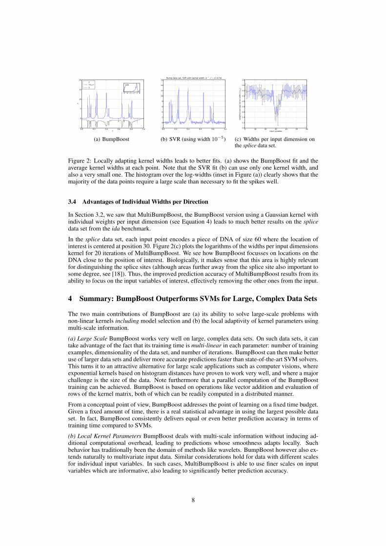
Masterarbeit am Institut fur Informatik der Freien Universitat Berlin,Arbeitsgruppe Intelligente Systeme und Robotik
In Zusammenarbeit mit der Arbeitsgruppe Maschinelles Lernen derTechnischen Universitat Berlin
Masterarbeit:
Big Data and Machine Learning: A Case
Study with Bump Boost
Maximilian AlberMatrikelnummer: 4452645
Eingereicht bei: Prof. Dr. Raul Rojas
Betreuer: Dr. Mikio Braun (TU Berlin)
Berlin, 19. Februar 2014
Abstract
With the increase of computing power and computing possibilities,especially the rise of cloud computing, more and more data accumu-lates, commonly named Big Data. This development leads to the needof scalable algorithms. Machine learning always had an emphasis onscalability, but few well scaling algorithms are known. Often, this prop-erty is reached by approximation. In this thesis, through a well struc-tured parallelization we enhance the Bump Boost and Multi BumpBoost algorithms. We show that with increasing data set sizes, the al-gorithms are able to reach almost perfect scalability. Furthermore, weinvestigate empirically how suitable Big-Data-frameworks, i.e. ApacheSpark and Apache Flink, are for implementing Bump Boost and MultiBump Boost.
Eidesstattliche Erklarung
Ich versichere hiermit an Eides Statt, dass diese Arbeit von niemand an-derem als meiner Person verfasst worden ist. Alle verwendeten Hilfsmittelwie Berichte, Bucher, Internetseiten oder ahnliches sind im Literaturverze-ichnis angegeben, Zitate aus fremden Arbeiten sind als solche kenntlichgemacht. Die Arbeit wurde bisher in gleicher oder ahnlicher Form keineranderen Prufungskommission vorgelegt und auch nicht veroffentlicht.
19. Februar 2015
Alber Maximilian
Acknowledgment
A thesis can hardly be written without any help. In the first place, I wouldlike to thank Mikio Braun for assisting me and for his valuable insights. Forher English lessons and for cross-reading my gratitude goes to Grete, for hisadvice to Marcin. Finally, I thank Nina for her company during the longwork hours and my mother for sustaining me.
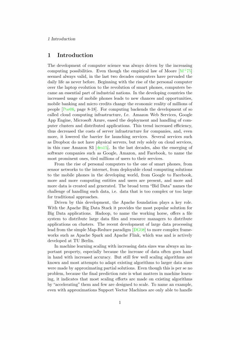
The development of computer science was always driven by the increasingcomputing possibilities. Even though the empirical law of Moore [M+75]seemed always valid, in the last two decades computers have pervaded thedaily life as never before. Beginning with the rise of the personal computerover the laptop evolution to the revolution of smart phones, computers be-came an essential part of industrial nations. In the developing countries theincreased usage of mobile phones leads to new chances and opportunities,mobile banking and micro credits change the economic reality of millions ofpeople [Por06, page 8-18]. For computing backends the development of socalled cloud computing infrastructure, f.e. Amazon Web Services, GoogleApp Engine, Microsoft Azure, eased the deployment and handling of com-puter clusters and distributed applications. This trend increased efficiency,thus decreased the costs of server infrastructure for companies, and, evenmore, it lowered the barrier for launching services. Several services suchas Dropbox do not have physical servers, but rely solely on cloud services,in this case Amazon S3 [dro15]. In the last decades, also the emerging ofsoftware companies such as Google, Amazon, and Facebook, to name themost prominent ones, tied millions of users to their services.
From the rise of personal computers to the one of smart phones, fromsensor networks to the internet, from deployable cloud computing solutionsto the mobile phones in the developing world, from Google to Facebook,more and more computing entities and users are present, and more andmore data is created and generated. The broad term “Bid Data” names thechallenge of handling such data, i.e. data that is too complex or too largefor traditional approaches.
Driven by this development, the Apache foundation plays a key role.With the Apache Big Data Stack it provides the most popular solution forBig Data applications. Hadoop, to name the working horse, offers a filesystem to distribute large data files and resource managers to distributeapplications on clusters. The recent development of large data processinglead from the simple Map-Reduce paradigm [DG08] to more complex frame-works such as Apache Spark and Apache Flink, which was and is activelydeveloped at TU Berlin.
In machine learning scaling with increasing data sizes was always an im-portant property, especially because the increase of data often goes handin hand with increased accuracy. But still few well scaling algorithms areknown and most attempts to adapt existing algorithms to larger data sizeswere made by approximating partial solutions. Even though this is per se noproblem, because the final prediction rate is what matters in machine learn-ing, it indicates that most scaling efforts are made on existing algorithmsby “accelerating” them and few are designed to scale. To name an example,even with approximations Support Vector Machines are only able to handle
1
1.1 Objectives of this Thesis
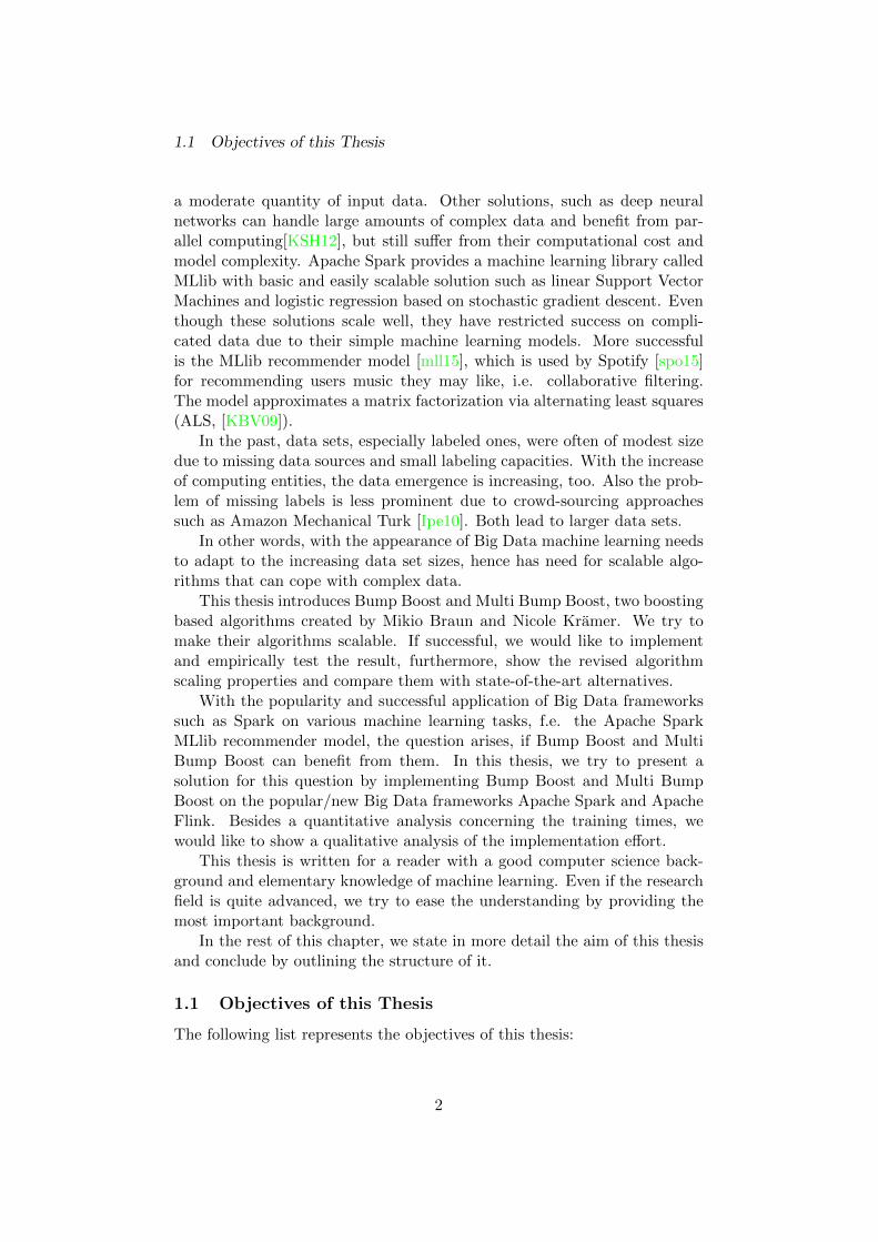
a moderate quantity of input data. Other solutions, such as deep neuralnetworks can handle large amounts of complex data and benefit from par-allel computing[KSH12], but still suffer from their computational cost andmodel complexity. Apache Spark provides a machine learning library calledMLlib with basic and easily scalable solution such as linear Support VectorMachines and logistic regression based on stochastic gradient descent. Eventhough these solutions scale well, they have restricted success on compli-cated data due to their simple machine learning models. More successfulis the MLlib recommender model [mll15], which is used by Spotify [spo15]for recommending users music they may like, i.e. collaborative filtering.The model approximates a matrix factorization via alternating least squares(ALS, [KBV09]).
In the past, data sets, especially labeled ones, were often of modest sizedue to missing data sources and small labeling capacities. With the increaseof computing entities, the data emergence is increasing, too. Also the prob-lem of missing labels is less prominent due to crowd-sourcing approachessuch as Amazon Mechanical Turk [Ipe10]. Both lead to larger data sets.
In other words, with the appearance of Big Data machine learning needsto adapt to the increasing data set sizes, hence has need for scalable algo-rithms that can cope with complex data.
This thesis introduces Bump Boost and Multi Bump Boost, two boostingbased algorithms created by Mikio Braun and Nicole Kramer. We try tomake their algorithms scalable. If successful, we would like to implementand empirically test the result, furthermore, show the revised algorithmscaling properties and compare them with state-of-the-art alternatives.
With the popularity and successful application of Big Data frameworkssuch as Spark on various machine learning tasks, f.e. the Apache SparkMLlib recommender model, the question arises, if Bump Boost and MultiBump Boost can benefit from them. In this thesis, we try to present asolution for this question by implementing Bump Boost and Multi BumpBoost on the popular/new Big Data frameworks Apache Spark and ApacheFlink. Besides a quantitative analysis concerning the training times, wewould like to show a qualitative analysis of the implementation effort.
This thesis is written for a reader with a good computer science back-ground and elementary knowledge of machine learning. Even if the researchfield is quite advanced, we try to ease the understanding by providing themost important background.
In the rest of this chapter, we state in more detail the aim of this thesisand conclude by outlining the structure of it.
1.1 Objectives of this Thesis
The following list represents the objectives of this thesis:
2
1.2 Organization of this Thesis
Scalability: The first and main purpose is to develop a parallelized andscalable variants of the Bump Boost and Multi Bump Boost algo-rithms. The theoretical results should be confirmed by testing themon sufficiently large data sets.
To be more precise, we expect from our solution, if possible, the com-plete same behavior as of the sequential solution. If not, the approxi-mations should be as accurate as possible. The solution should exhibita good scaling behavior, i.e. when parallelizing the same work on ninstances, the run time should be approximately a n-th of the sequen-tial one and the overall run time should scale linearly with increasingdata set sizes.
Big Data frameworks: The second objective is to examine the suitabilityof Apache Spark and Apache Flink for implementing Bump Boostand Multi Bump Boost. Again, next to the empirical evaluation, theresulting programs should be tested on their scaling properties.
To be more accurate, the final solution should be easily understandableand comprehensible. The adaption from the traditional programmingmodel to the semantics imposed by the frameworks should be as smallas possible. Finally, we expect the solutions to scale well, i.e. with thesame criteria as in the first objective.
1.2 Organization of this Thesis
The thesis is structured as follows:
Chapter 2: Big DataThis chapter clarifies our understanding of Big Data and sketches howBig Data influences machine learning and this thesis.
Chapter 3: Scaling and ParallelizationThe broad terms scaling and parallelization are introduced and theirmeaning in our context is specified. In addition, we present the basictheory and principles of parallelization.
Chapter 4: Machine Learning and Bump BoostAfter giving an introduction to machine learning and the theoreticalbackground of Bump Boost and Multi Bump Boost, the algorithmsthemselves are described. The chapter concludes with the descriptionof the parallelized Bump Boost and Multi Bump Boost algorithms.
Chapter 5: Related WorkIn this chapter we show related work in the field of machine learning.
Chapter 6: Tools and FrameworksThe used programming tools and frameworks, for example the ApacheBig Data stack, are described in this chapter.
3
1.2 Organization of this Thesis
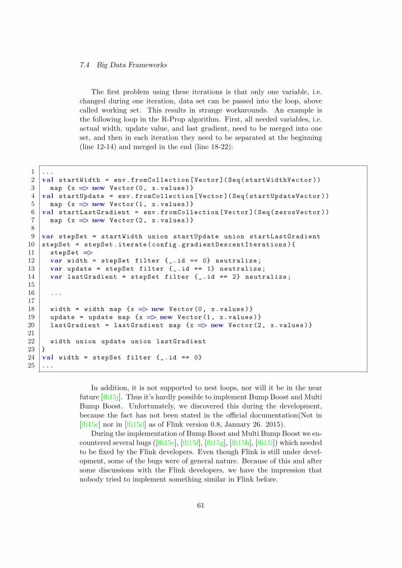
Chapter 7: ImplementationsThe first part of this chapter depicts our implementation of BumpBoost and Multi Bump Boost. The second part is on how we try torealize a solution with Apache Spark and Apache Flink.
Chapter 8: Competitive SolutionsThis chapter treats the algorithms we used for comparison.
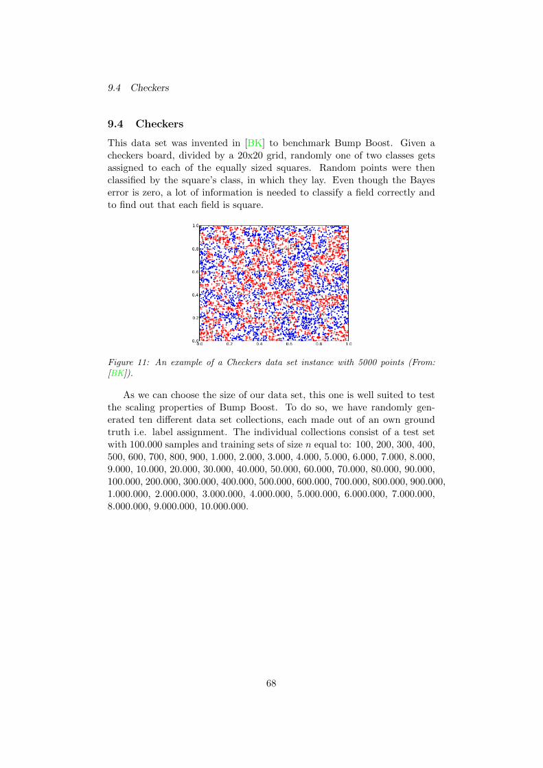
Chapter 9: Data SetsThe data sets used for our experiments are given in this chapter.
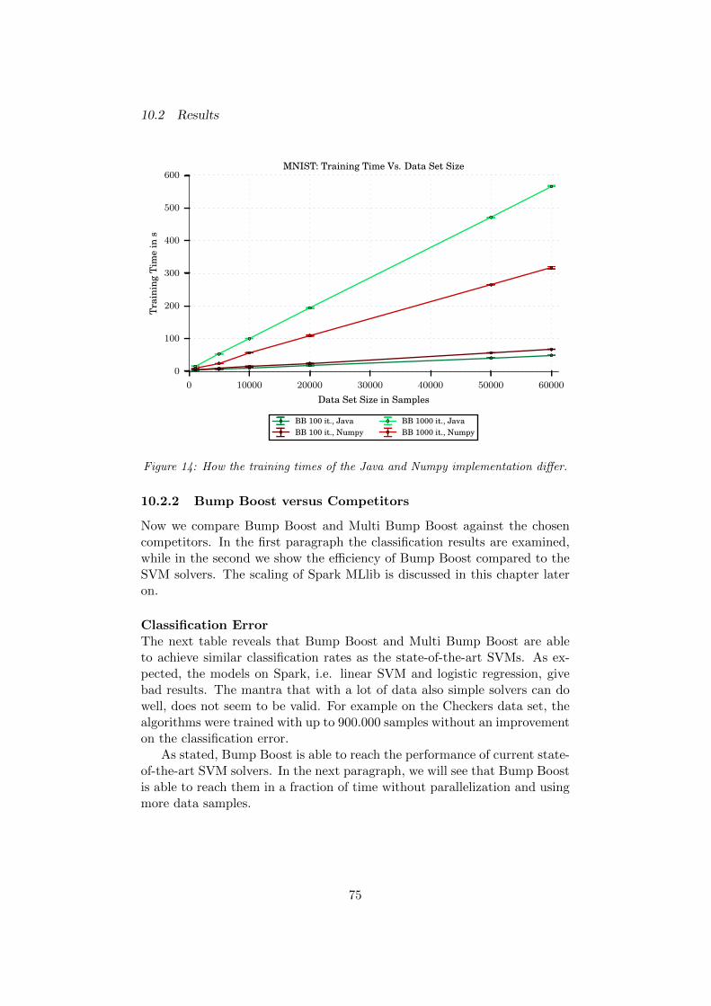
Chapter 10: Experiments and ResultsAfter introducing our experiment setups, we show and describe thequantitative results of this thesis.
Chapter 11: Conclusion and PerspectiveIn this final chapter we conclude and give a perspective on futurequestions.
Appendix:In the appendix we provide the original, but never published, paperon Bump Boost and describe the content of the enclosed DVD.
4
2 Big Data
2 Big Data
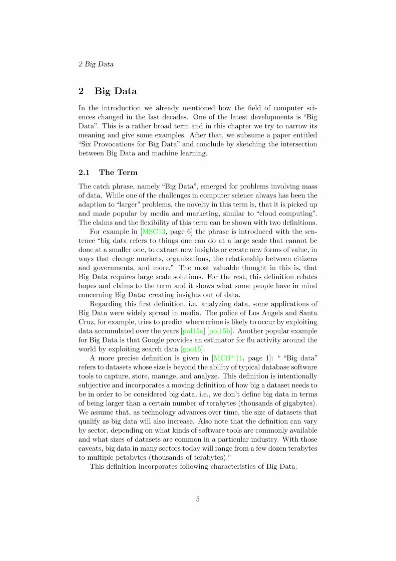
In the introduction we already mentioned how the field of computer sci-ences changed in the last decades. One of the latest developments is “BigData”. This is a rather broad term and in this chapter we try to narrow itsmeaning and give some examples. After that, we subsume a paper entitled“Six Provocations for Big Data” and conclude by sketching the intersectionbetween Big Data and machine learning.
2.1 The Term
The catch phrase, namely “Big Data”, emerged for problems involving massof data. While one of the challenges in computer science always has been theadaption to“larger”problems, the novelty in this term is, that it is picked upand made popular by media and marketing, similar to “cloud computing”.The claims and the flexibility of this term can be shown with two definitions.
For example in [MSC13, page 6] the phrase is introduced with the sen-tence “big data refers to things one can do at a large scale that cannot bedone at a smaller one, to extract new insights or create new forms of value, inways that change markets, organizations, the relationship between citizensand governments, and more.” The most valuable thought in this is, thatBig Data requires large scale solutions. For the rest, this definition relateshopes and claims to the term and it shows what some people have in mindconcerning Big Data: creating insights out of data.
Regarding this first definition, i.e. analyzing data, some applications ofBig Data were widely spread in media. The police of Los Angels and SantaCruz, for example, tries to predict where crime is likely to occur by exploitingdata accumulated over the years [pol15a] [pol15b]. Another popular examplefor Big Data is that Google provides an estimator for flu activity around theworld by exploiting search data [goo15].
A more precise definition is given in [MCB+11, page 1]: “ “Big data”refers to datasets whose size is beyond the ability of typical database softwaretools to capture, store, manage, and analyze. This definition is intentionallysubjective and incorporates a moving definition of how big a dataset needs tobe in order to be considered big data, i.e., we don’t define big data in termsof being larger than a certain number of terabytes (thousands of gigabytes).We assume that, as technology advances over time, the size of datasets thatqualify as big data will also increase. Also note that the definition can varyby sector, depending on what kinds of software tools are commonly availableand what sizes of datasets are common in a particular industry. With thosecaveats, big data in many sectors today will range from a few dozen terabytesto multiple petabytes (thousands of terabytes).”
This definition incorporates following characteristics of Big Data:
5
2.2 Provocations for Big Data
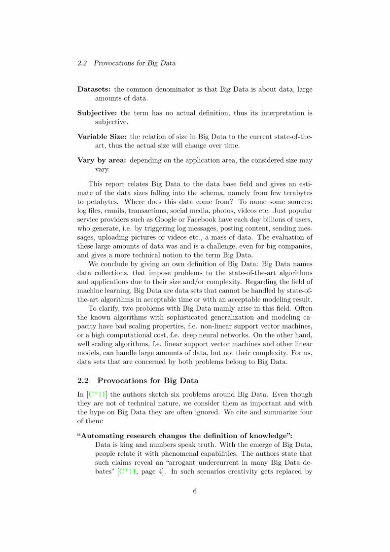
Datasets: the common denominator is that Big Data is about data, largeamounts of data.
Subjective: the term has no actual definition, thus its interpretation issubjective.
Variable Size: the relation of size in Big Data to the current state-of-the-art, thus the actual size will change over time.
Vary by area: depending on the application area, the considered size mayvary.
This report relates Big Data to the data base field and gives an esti-mate of the data sizes falling into the schema, namely from few terabytesto petabytes. Where does this data come from? To name some sources:log files, emails, transactions, social media, photos, videos etc. Just popularservice providers such as Google or Facebook have each day billions of users,who generate, i.e. by triggering log messages, posting content, sending mes-sages, uploading pictures or videos etc., a mass of data. The evaluation ofthese large amounts of data was and is a challenge, even for big companies,and gives a more technical notion to the term Big Data.
We conclude by giving an own definition of Big Data: Big Data namesdata collections, that impose problems to the state-of-the-art algorithmsand applications due to their size and/or complexity. Regarding the field ofmachine learning, Big Data are data sets that cannot be handled by state-of-the-art algorithms in acceptable time or with an acceptable modeling result.
To clarify, two problems with Big Data mainly arise in this field. Oftenthe known algorithms with sophisticated generalization and modeling ca-pacity have bad scaling properties, f.e. non-linear support vector machines,or a high computational cost, f.e. deep neural networks. On the other hand,well scaling algorithms, f.e. linear support vector machines and other linearmodels, can handle large amounts of data, but not their complexity. For us,data sets that are concerned by both problems belong to Big Data.
2.2 Provocations for Big Data
In [C+11] the authors sketch six problems around Big Data. Even thoughthey are not of technical nature, we consider them as important and withthe hype on Big Data they are often ignored. We cite and summarize fourof them:
“Automating research changes the definition of knowledge”:Data is king and numbers speak truth. With the emerge of Big Data,people relate it with phenomenal capabilities. The authors state thatsuch claims reveal an “arrogant undercurrent in many Big Data de-bates” [C+11, page 4]. In such scenarios creativity gets replaced by
6
2.3 Big Data and Machine Learning
the worship of data, data that lacks the “regulating force of philoso-phy.” [C+11, page 4] In other words, we should not forget restrictionsimposed to Big Data and the related tools.
“Claims to objectivity and accuracy are misleading”:“Interpretation is at the center of data analysis. Regardless of the sizeof a data set, it is subject to limitation and bias. Without those biasesand limitations being understood and outlined, misinterpretation isthe result. Big Data is at its most effective when researchers takeinto account the complex methodological processes that underlie theanalysis of ... data.” [C+11, page 6]
“Just because it is accessible doesn’t make it ethical”:By tracking public Facebook user profiles, scientists of Harvard tried toanalyze changing characteristics over time. Even though, the releaseddata was anonymized, quickly it was shown that deanonymizing ispossible, compromising people’s privacy. Other studies give furtherexamples of how individuals can deanomyzed with enough data, f.e.[SH12]. Big Data abstracts reality, thus one should not forget to con-sider that “there is a considerable difference between being in publicand being public” [C+11, page 11-12] and where the data comes from.
“Limiting access to Big Data creates new digital divides”:Collecting, cleansing and analyzing data is a tedious task. Besides, thisdata is a valuable source. Resulting, most companies restrict access totheir resources. F.e. Twitter offers access to nearly all Tweets only toa selected number of firms and researchers. In such cases a scientistwith access to such data is privileged over others. Next to this accessquestion, handling Big Data imposes requirement to specific knowledgeand infrastructure, which again is a potential divide.
2.3 Big Data and Machine Learning
Given this introduction to Big Data, the question of how this relates tomachine learning is left. First of all, data sets used in machine learningtasks are often inspired by real world scenarios and their accumulated data.In future, more tasks with large data sets will arise as more data will becollected. An example is the Netflix competition of 2006, where researcheswere challenged to develop a recommender system using a data set with 100million samples [BL07].
Besides the sole size, data sets with increased complexity were released.The popular ImageNet data set [DDS+09] with millions of images is anexample. The task is to localize and/or classify objects of 1000 classesinside these pictures. Each year a competition called “Large Scale VisualRecognition Challenge” is held to determine the state-of-the-art.
7
2.3 Big Data and Machine Learning
Both examples fall into our definition, because size and complexity forcedand force researcher to create new solutions. But while in these two cases theamount of data may seem justified, due to the complex task, in other casesmore data might not lead to new insights. Depending on the complexity, thegain due to this additional data might be negligible. In contrast, additionaldata should not harm the prediction success, contrariwise, more data usuallyleads to better generalization.
The scaling properties of popular machine learning algorithms, such asf.e. Support Vector Machines, are a problem when data set sizes are toolarge. As a solution, data sets can be sampled to one with a smaller size,but if the underlying problem is too complex the machine learning algorithmmight be not able to generalize well.
In this thesis, we do not want to examine such questions, i.e. how muchdata is really needed by an algorithm to generalize well or what the benefitof more data might be. Instead we want to emphasize on the scaling of thealgorithms, i.e. of Bump Boost and Multi Bump Boost.
8
3 Scaling and Parallelization
3 Scaling and Parallelization
This section gives an overview over the broad terms scaling and paralleliza-tion. We aim to clarify what they mean in our context and to introducesome theoretical constraints and criteria.
3.1 Scalability
As “Big Data” “scalability” is not well defined, i.e. there is no generally-accepted definition [Hil90]. The term itself is related to the word scale andintuitively we connect it to a desirable result after a change of scale in theproblem solving capacity or the problem size itself.
For this work we define two notions of scalability. For both we under-stand as problem the training time of an algorithm and as a worker anindependent instance, i.e. process.
The first one is related to the problem solving capacity i.e. in our casewe would like the runtime to decrease as the number of workers increases.To be more precise, we would like to have with n workers a speedup of n(see next section), i.e. with n workers the problem should be solved in ntimes as fast as one worker is able to.
The second one is related to the problem size itself, i.e. generally thenumber of data samples in the training set. Again to be more precise wewould like to have the runtime doubling, if the problem size doubles and thesame problem solving setup tackles them.
3.2 Parallel Computing
Under parallel computing we understand the execution of two or more dif-ferent calculations at the same time. In the further we want to restrict usand assume that these parallel calculations belong to the same algorithm.
“Parallelization” in this context means the execution of an algorithm inparallel instead of sequential manner. The goal of this modification canbe a runtime improvement or to enable an algorithm handling larger inputdimensions by using more computational power.
The rest of this section describes the most concerning theory, followedby difficulties imposed by parallel computing. Finally, the major ways toparallelize a computer program are shown.
3.2.1 Theory
Theoretical Constraints
At first we would like to introduce the notion of speedup S(N). It is
9
3.2 Parallel Computing
defined by [Geb11, page 15/16]:
S(N) =T (1)
T (N)(1)
for N parallel computing instances, where T (1) is the algorithm time usinga single one and T (N) is the algorithm time using N .
In a desirable situation, we have no overhead and the algorithm is fullyparallelizable, thus T (N) = T (1)/N holds. Which results in S(N) = N .
A theoretical limit for the speedup is set by Amdahl’s law [Amd67].Assuming the parallelizable fraction of an algorithm is f , thus the serial oneis 1− f , then the time on N instances can be written as:
TAmd(N) = T (1)((1− f) +1
N∗ f) (2)
This implies the maximum speedup of:
SAmd(N) =1
(1− f) + 1N ∗ f
(3)
So to say, the goal must be a big parallelizable fraction of the algorithm,i.e. 1 − f << f/N , to gain a real speedup. Another insight is that thespeedup saturates when N gets large:
21 22 23 24 25 26 27 28 29 210 211 212
Parallel Instances Count N
0
2
4
6
8
10
12
14
16
18
20
Spee
dup
Amdahl’s Law
Parallel portion f:50759095
Figure 1: Examples how Amdahl’s law evolves with increasing number of parallelinstances.
The drawback in Amdahl’s law is the fixed input size. Generally, inreal world settings the computation can be solved more efficiently when
10
3.2 Parallel Computing
the problem, i.e. data, size increases. This is addressed by Gustafson-Barsis’s law [Gus88]. Given the execution time on N computing instancesthe computing time on N instances can be written as:
TGB(N) = T (N) ∗ ((1− f) + f) (4)
We can describe the computing time on one instance as:
TGB(1) = T (N) ∗ ((1− f) +N ∗ f) (5)
This results in the maximum speedup of:
SGB(N) = (1− f) +N ∗ f = 1 + (N − 1) ∗ f (6)
28 29 210 211 212
Parallel Instances Count N
0
500
1000
1500
2000
2500
3000
3500
4000
Spee
dup
Gustafson-Barsis’s Law
Parallel portion f:50759095
Figure 2: Examples how Gustafson-Barsis’s law evolves with increasing number ofparallel instances.
“... with a distributed memory-computer, larger size problems can besolved. This model proves to be adapted to distributed-memory architec-tures and explains the high performance achieved with these problems.”[Roo00, page 228]
Both theories give quite different results due to their viewpoint. Am-dahl’s law treats the problem size as constant and only the parallel fractioncan be reduced, while in Gustafson-Barsis’s law the time of the parallelfraction is fixed and the sequential solution scales with N .
Computation Taxonomy
11
3.2 Parallel Computing
There are several ways to describe computation devices. One of the mostpopular is Flynn’s Taxonomy [Fly66]. Its main focus is on how programinstructions and program data relate to each other:
Single Instruction Stream, Single Data Stream (SISD):This class of computers is characterized by a strict scheme in which asingle instruction operates on a single data element at the time. Thismodel fits best with the traditional Von Neumann computing model[VN93]. Early single core processors belong to this class.
Single Instruction Stream, Multiple Data Streams (SIMD):When several processing units operate on several data elements andall is supervised by a single control unit, a computing device belongsto this class. An example are vector processors, which are used f.e. inGPUs.
Multiple Instruction Streams, Single Data Stream (MISD):The characteristic of this class is given by several instructions, thatare performed simultaneously on the same data. There can be twointerpretations: “A class of machines that would require distinct pro-cessing units that would receive distinct instructions to be performedon the same data. This was a big challenge for many designers andthere are currently no machines of this in the world.” [Roo00, page 3]In a more broad definition pipeline processors, i.e. processors, whichapply different instructions to one single data stream in a pipeline inone time instance, can be seen as SIMD, if we classify the data streamas one piece of data. [Roo00, page 3]
Multiple Instruction Streams, Multiple Data Streams (MIMD):Typical multiprocessors or multi computer systems belong to this lastclass, which is described by several instructions that perform on dif-ferent data elements in the same time.
3.2.2 Problems
Not all algorithms are parallelizable. Most intuitively two program frag-ments need to be scheduled in sequential manner, if one’s input dependson the output of the other. According to Amdahl’s law, no program canexecute faster than the longest sequential part. This part is given by the socalled critical path, i.e. the longest path of sequential program fragments.
Next to some other possible and less important dependencies, f.e. controldependencies, where execution of an instruction depends on some (variable)data [Roo00, page 115], data dependencies restrict the parallelization suc-cess. They are formally described by the Bernstein’s conditions [Ber66].
12
3.2 Parallel Computing
According to them, two program Pi, Pj fragments, with the input and out-put variables Ii, Ij and Oi, Oj , are independent, i.e. they can be executedin parallel, if the following conditions hold:
Ii ∩Oj = ∅Ij ∩Oi = ∅Oi ∩Oj = ∅
(7)
The last condition represents the case, in which one fragment wouldoverwrite the output of another.
Following to this input/output relations, it is possible to build a di-rected, acyclic graph representing the data flow and possible parallelizationopportunities.
Beside this theoretical barrier, the implementation of in-parallel executedprograms can be challenging. Even though the single parallel instances ex-ecute their program independently, their results need to get combined to-gether. The major problems are caused by communication, data access anddata consistency between the parallel instances. F.e. deadlocks, lifelocks,race conditions can arise, to name some well known problems.
In some theory, f.e. in Amdahl’s law, there is no notion of overhead,i.e. effort induced by parallel computing. This overhead generally increaseswith more parallel instances. Thus, more computing instances do not resultnecessarily in a faster execution. Usually this overhead is caused by thebigger communication effort. We speak of parallel slowdown, when moreparallel instances solve a problem more slowly than less instances.
3.2.3 Parallelism Characteristics
Programs can be parallelized on different levels. Some examples are Bit-parallelism, where single Bit-operations are carried out in parallel by theCPU, instruction-parallelism, where instruction are performed in parallel,and program-parallelism, where different programs are scheduled in the sametime instant. [RR13, page 110]
The effort can further be classified by the characteristics of the parallelcomputations. F.e. in data parallelism several computing units performthe same operations on the different data parts, whereas control parallelismis given when simultaneously performing several different instructions ondifferent data. The former usually is arising on SIMD or MIMD computersystems, the later on MIMD environments. [Roo00, page 117-199]
In practice, data parallelism can be achieved by programming GPU de-vices or using data parallel programming languages s.a. Fortran 90 [RR13,page 112]. While control parallelism is given in multi process-, thread-,and/or host-programs.
Another characteristic of parallel programs is the way in which they com-municate. There are two basic possibilities. The first is to communicate via
13
3.2 Parallel Computing
messages, i.e. communication links, the second is a shared memory space.While message passing models highly depend on the implementation andcan be synchronous as asynchronous, shared memory is tightly related tothe underlying communication and consistency models. In this case syn-chronization is a needed characteristic and a likely performance impact.[Roo00, page 120-123]
The practical realization generally is coupled to the operating systemcapabilities. Network stacks or local inter-process message passing interfacesfor message communication or shared memory between local processes areusual features of modern operating systems.
14
4 Machine Learning and Bump Boost
4 Machine Learning and Bump Boost
In this chapter we give an introduction to the machine learning and thebackgrounds that concern us most. Besides that, we present an algorithmcalled Support Vector Machine and conclude with an in-depth descriptionof the Bump Boost algorithms and their parallel variants.
4.1 Background
The background knowledge is organized as follows. After introducing adefinition for machine learning and the relationship to other science fields,we confine and specify the in this work treated sub-field of machine learning.At last we describe several basic algorithm techniques.
4.1.1 Machine Learning
To generally describe machine learning we use two citations. “MachineLearning is the field of scientific study that concentrates on induction al-gorithms and on other algorithms that can be said to “learn.”” [KP] Theterm “learning” can be further clarified: “In the broadest sense, any methodthat incorporates information from training samples ... employs learning.”[DHS99, page 16] Summarizing: machine learning is the field of study con-centrated on algorithms of whose future behavior is influenced, i.e. learned,from training samples, i.e. data.
In order to learn, a notion of “what to learn” is needed, which can bereally subjective. Given this “what to learn” we would like to measure howwell our algorithm learned it. This usually is done with some objectivefunction, which measures the gap between realized and desired behavior.Thus the goal is to minimize this gap, i.e. the objective function. This can bedone in several ways and often it is the actual minimization of mathematicalfunction.
Caused by the use of data and its characteristics as the computationalproblems machine learning can be seen as subfield of Statistics and Com-puter Science. Next to that, the field is tightly coupled to fields of ArtificialIntelligence and mathematical optimization. The first is a source for algo-rithms and ideas, the second is a toolbox to optimize the algorithms andfunctions. In 4.1.4 some basic optimization examples are listed.
For this work we would like to restrict our view on machine learninga bit more. We assume that the algorithm gets provided some train setXtrain which consists of Ntrain samples. For each sample a correct result orlabel, see next section, is provided in the set Ytrain. By using some objectivefunction the algorithm itself can measure the gap between its prediction andthe desired result. The result of this training procedure is a prediction model.Finally, there is a test set Xtest which is never provided to the algorithm or
15
4.1 Background
model for learning, its solely purpose is to compare the predictions of themodel with the actual results Ytest and so to rate the algorithm predictionperformance.
4.1.2 Supervised Learning
Depending on the feedback, learning itself can be classified [DHS99, page16-17]:
Supervised Learning: For each training or test result a correct label/re-sult or a cost for it will be provided to the algorithm.
Unsupervised Learning: There are no labels or results for the data sam-ples. In this case the algorithms usually try to cluster similar samples(f.e. the k-means algorithm) or to find pattern in the data (f.e. auto-encoders [EBC+10]).
Reinforcement Learning: For each data sample the algorithm only getsbinary feedback, thus if the answer is correct or not. In contrast, thefeedback in supervised learning usually is enriched by the knowledgeof how wrong an answer is or what the desired one would be.
In this work we only use supervised learning.
4.1.3 Regression and Classification
In the case of supervised learning we can further distinct between regressionand classification tasks. In regression tasks the result is not constrained andcommonly it is a real value. In contrast, classification tasks provide a setof labels and each data sample belongs to one. Classification can be viewedas subproblem of regression. Thus a regression algorithm does theoreticallywork on a classification problem, vice versa this is not the case.
The most popular and easiest case of classification consists of two cases.All the other so called multi-class classification tasks can be modified into atwo class problem, i.e. “Is this sample part of class X?”.
In this work we use only two class problems, because it is the mostcommon denominator for classification algorithms.
4.1.4 Gradient Methods
Let us assume some data X, the desired result vector Y , some predictionfunction f with a parameter set θ and a cost function C(Y, f(X; θ)). Nowwe would like to choose the optimal parameter setting popt ∈ θ, i.e. thesetting with the smallest cost.
One ineffective and usually infeasible way to find popt would be to try allthe possible instances. Another, inspired from Artificial Intelligence, could
16
4.1 Background
be a genetic algorithm, i.e. keeping a “population” of parameter settings,based on some fitness function drop some and alter some other until a sat-isfying result is reached. But the most common one is to use the gradient∂C(Y,f(X;θ))
∂θ . In some easy cases finding the optimum will be solvable ana-lytically, in most, usually non-linear ones, not.
In this cases gradient descent methods can be used. The general ap-proach is to start with a random parameter setting p, to compute thegradient g, based on the result to modify p, f.e. for a single parameterpnew = p− l ∗ g with some “learning rate” l, and then repeat until some stopcriterion is satisfied.
There are several different approaches. Some, for example, take intoaccount the second gradient. Most of them have in common that they cannot guarantee to find popt. Here we present R-Prop [RB93] which is used byMulti Bump Boost (see 4.3.1):
The special characteristic is that it modifies the current parameter set-ting solely on the knowledge of the gradient sign change. At the beginningsome random or static value for p will be chosen as some static one for the“update” value u. Umin and Umax are the minimum and maximum size forthe update value u and the values 0 < η− = 0.5 < 1 < η+ = 1.2 are setempirically. In each step t the parameter setting will be updated accordingto the gradient g as follows. “Zt” denotes values “Z” at iteration step t:
ut+1 =
min(ut ∗ η+, Umax) if gt ∗ gt−1 > 0
max(ut ∗ η−, Umin) if gt ∗ gt−1 < 0
ut otherwise
(8)
∆pt = −ut ∗ sgn(gt) (9)
pt+1 = pt + ∆pt (10)
The informal behavior is following the gradient descent and increasingthe speed as long as the gradient sign does not change. If it does, decreasethe speed.
4.1.5 Cross Validation
Usually, not all parameters of a model are selected with a gradient descentor another automatic method. Those parameters are set by hand by thedeveloper. Examples would be the number of hidden units in a neural net-work etc. In order to select them as objectively as possible, m-fold crossvalidation is often a good choice.
“Here the training set is randomly divided into m disjoint sets of equalsize n/m, where n is again the total number of patterns in D. The classifieris trained m times, each time with a different set held out as a validation set.
17
4.1 Background
The estimated performance is the mean of these m errors.” [DHS99, page483/484] Important to notice is that train and validation sets are alwaysdisjoint and that D would never incorporate the actual test set.
Given np parameter settings, to each of them the above procedure wouldbe applied. The setting with the lowest error would be the final choice andused to create the final model by training on the whole training set.
This technique is used to find the best parameters for Support VectorMachines in this work.
4.1.6 Boosting
A special technique to join so called weak learners to an effective predictor iscalled “Boosting”. Weak learners’ characteristic is that they are only slightlybetter than chance. In principle, also a better learner could be used, butthan the effect of Boosting is not as important.
The general setup is to choose a weak learner, train it on the training setand then train the“successive ... classifiers with a subset of the training datathat is “most informative” given the current set of ... classifiers” [DHS99,page 476] (Note: Boosting is not restricted to classification tasks.). In gen-eral, this means that the successive training will be done on the training setparts that are predicted worse by the already selected learners.
The final prediction is done together by all learned models. How thosevotes are joint is part of the actual boosting algorithm, but usually theweighted votes are joint to a final one.
A popular example for Boosting is algorithm of Viola and Jones [VJ01]using AdaBoost [FS95], which uses Haar-like features to rapidly detect com-plex objects like faces.
In the next sub chapter we will present the Bump Boost algorithm, whichis based on Boosting.
4.1.7 Kernel methods
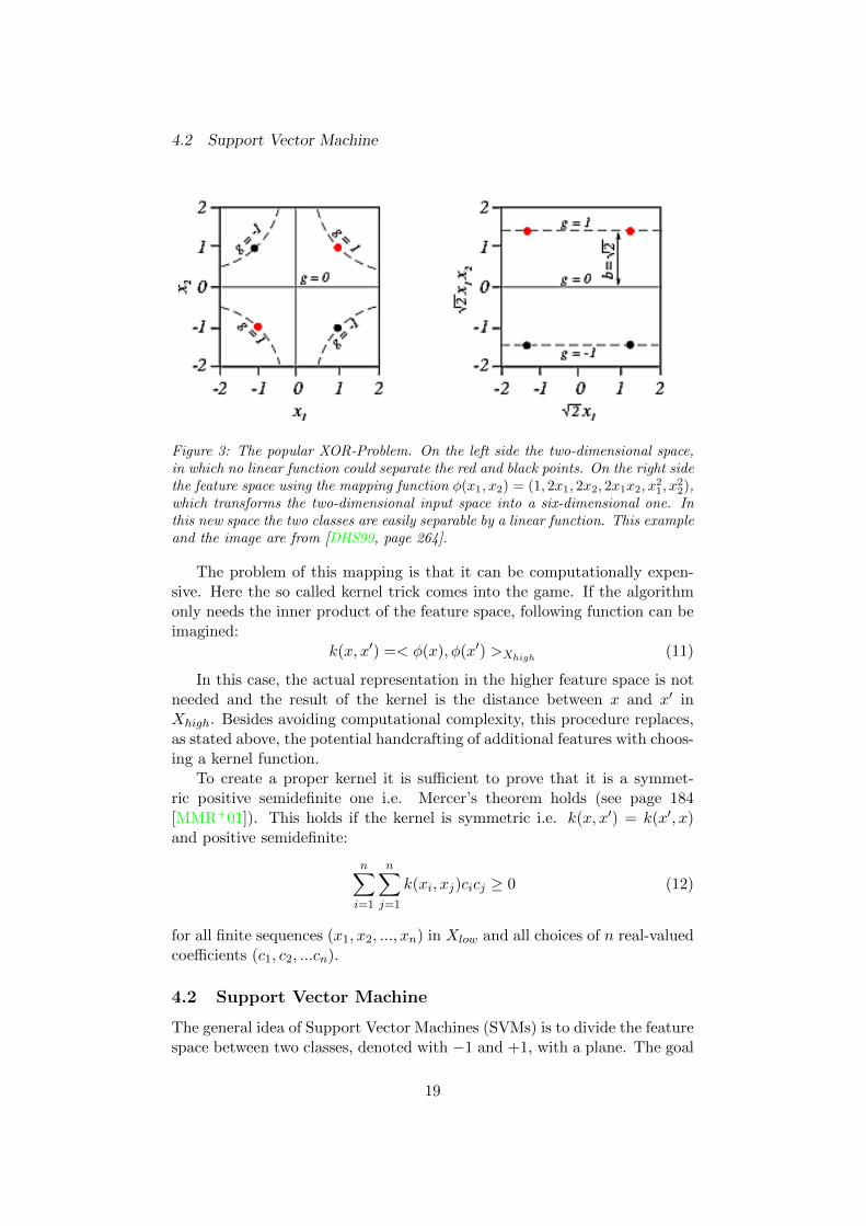
Often, the given features are in raw form and could be separated in moreuseful ones, i.e. transformed into a higher feature space. High, in this con-text, means higher dimensional. This could be done manually or preferablyby choosing some function φ(Xlow)→ Xhigh.
A popular usage example are Support Vector Machines (see 4.2). Theytry to separate the samples of class 1 from the samples of class 2 with a(hyper-)plane. By mapping the input space into a higher dimensional one,this task can be eased, because certain features can get separable there,while in the original space they are not.
18
4.2 Support Vector Machine
Figure 3: The popular XOR-Problem. On the left side the two-dimensional space,in which no linear function could separate the red and black points. On the right sidethe feature space using the mapping function φ(x1, x2) = (1, 2x1, 2x2, 2x1x2, x
21, x
22),
which transforms the two-dimensional input space into a six-dimensional one. Inthis new space the two classes are easily separable by a linear function. This exampleand the image are from [DHS99, page 264].
The problem of this mapping is that it can be computationally expen-sive. Here the so called kernel trick comes into the game. If the algorithmonly needs the inner product of the feature space, following function can beimagined:
k(x, x′) =< φ(x), φ(x′) >Xhigh(11)
In this case, the actual representation in the higher feature space is notneeded and the result of the kernel is the distance between x and x′ inXhigh. Besides avoiding computational complexity, this procedure replaces,as stated above, the potential handcrafting of additional features with choos-ing a kernel function.
To create a proper kernel it is sufficient to prove that it is a symmet-ric positive semidefinite one i.e. Mercer’s theorem holds (see page 184[MMR+01]). This holds if the kernel is symmetric i.e. k(x, x′) = k(x′, x)and positive semidefinite:
n∑
i=1
n∑
j=1
k(xi, xj)cicj ≥ 0 (12)
for all finite sequences (x1, x2, ..., xn) in Xlow and all choices of n real-valuedcoefficients (c1, c2, ...cn).
4.2 Support Vector Machine
The general idea of Support Vector Machines (SVMs) is to divide the featurespace between two classes, denoted with −1 and +1, with a plane. The goal
19
4.2 Support Vector Machine
thereby is to maximize the distance between the plane and nearest points ofeach class. This distance is called margin and the plane, that maximizes it,maximum-margin (hyper-)plane.
Figure 4: This image shows a two-class separation problem. The optimal hyper-plane lies exactly in the middle between the two nearest points of the two classes.In this case, the solid dots would represent the Support Vectors (see below). Thisexample and the image are from [DHS99, page 262].
This algorithm and its soft margin extension were introduced by Vapnikand Cortes in [CV95].
Given this plane (w, b), a point can be easily classified to class one, ifw · x− b > 0 holds, else it is of class two.
The optimization problem maximizing the margin can be written as:
argmin(w,b)
1
2‖w‖2
subject to ∀i = 1, ..., n : yi(w · xi − b) ≥ 1
(13)
The ≥ 1 guarantees that all points are outside of the margin.The original form, called primal form, can be rewritten to the dual form
by exploiting the facts that ‖w‖2 = w · w and w =∑n
i=1 αiyixi [CV95,Equation 14]:
argmaxα
n∑
i=1
αi −1
2
n∑
i=1
n∑
j=1
αiαjyiyjx>i xj
subject to ∀i = 1, ..., n : αi ≥ 0
constrained byn∑
i=1
αiyi = 0
(14)
20
4.2 Support Vector Machine
The plane can be explicitly expressed by w =∑n
i=1 αiyixi. All the pointsxi with αi 6= 0 are called “Support Vectors”.
This form also shows that the kernel trick (see 4.1.7) can be applied byreplacing the inner product x>i xj with a valid kernel k(xi, xj) leading to anon-linear SVM:
argmaxα
n∑
i=1
αi −1
2
n∑
i=1
n∑
j=1
αiαjyiyjk(xi, xj)
subject to ∀i = 1, ..., n : αi ≥ 0
constrained by
n∑
i=1
αiyi = 0
(15)
The constraint that no point may lie inside the margin can be too re-strictive, f.e. if the data is noisy. Due to this reason, a slack variable ξ, inthis case as linear penalty, was introduced:
argmin(w,b,ξ)
1
2‖w‖2 + C
n∑
i=1
ξi
subject to ∀i = 1, ..., n : yi(w · xi − b) ≥ 1− ξi, ξi ≥ 0
(16)
Depending on the regularization parameter C the exception on the mar-gin constraints are more or less punished.
In the dual form the linear penalty vanishes except one key point:
argmaxα
n∑
i=1
αi −1
2
n∑
i=1
n∑
j=1
αiαjyiyjx>i xj
subject to ∀i = 1, ..., n : 0 ≤ αi ≤ C
constrained byn∑
i=1
αiyi = 0
(17)
4.2.1 Implementation
Left with these mathematical optimization problems out of the box solversfor these can be used, i.e. quadratic program solvers. These methods canbe quite complex and the programs expensive.
Another neat and for SVMs-specialized approach is the “Sequential Min-imal Optimization”-algorithm (SMO) [P+98] invented by John Platt. Bybreaking down the problem to two Lagrange multipliers and solving it an-alytically, the algorithm reduces the optimization complexity. This is donefor all Lagrange multiplier as long as they violate the Karush-Kuhn-Tuckerconditions.
Linear SVMs can also be solved efficiently with gradient descent methods(see 4.1.4).
21
4.3 Bump Boost
4.3 Bump Boost
Now we would like to introduce the central algorithms of this thesis. Theywere invented by Mikio Braun and Nicole Kramer in [BK]. The paper wasnever published, therefore we provide a copy in the appendix C.
Bump Boost and Multi Bump Boost can be used for classification andregression. The algorithm remains the same. Due to the used data sets,only classification is mentioned.
This section is organized as follows. First we describe the algorithms ofBump Boost and Multi Bump Boost. Then we state some of their charac-teristics. We conclude with proposals for a parallelized Bump Boost andMulti Bump Boost version.
4.3.1 The Algorithm
Lets begin with the final prediction model. Based on m learned, and socalled, bumps, the final prediction function is defined for x ∈ Rd as follows:
f(x) =m∑
i=1
hi ∗ kwi(ci, x)
with kwi(x, x′) = exp
−
d∑
j=1
(x− x′)2wj
(18)
One bump is described by the triple center, width, and height ∀i ∈1, ..., n : (ci, wi, hi); ci, wi ∈ Rd;hi ∈ R.
The kernel k could also be replaced: the algorithm “does not fit all kindsof kernels, but is specialized to “bump-like” kernels like the Gaussian kernelor the rational quadratic kernel which have a maximum when the two pointscoincide.” [BK, page 2] In this paper, we use only this Gaussian one.
Both algorithms, Bump Boost and Multi Bump Boost, as training inputget a feature matrix X ∈ Rnxd and a result vector Y ∈ Rn with n-samplesand base on Boosting (see 4.1.6), namely l2-Boosting [BY03]. The generalalgorithm for l2-Boosting is as follows:
Initialize residuals r ← Y , learned function f(x)← 0;for i = 1, ...,m do
Learn a weak learner hi which fits (X1, r1), ..., (Xn, rn);Add hi to learned function: f ← f + hi;Update the residuals: rj ← rj − hi(Xj) ∀j ∈ 1, ..., n;
end
22
4.3 Bump Boost
In our case, the weak learners are Gaussian bumps fitted to the residuals.The following plots show an example of learning bumps. The learned datais the Heavisine function from the Donoho test set [DJKP95]. A noise levelof 0.01 is applied on the 500 points:
0.0 0.2 0.4 0.6 0.8 1.0
−8
−6
−4
−2
0
2
4
6
Ground Truth
(a) The data set.
0.0 0.2 0.4 0.6 0.8 1.0
−8
−6
−4
−2
0
2
4
6
Ground TruthPrediction after 100. Iter.Residuals
(b) Learned function after 100. iterations.
0.0 0.2 0.4 0.6 0.8 1.0
−8
−6
−4
−2
0
2
4
6
r at Iter. = 1r at Iter. = 2Bump at Iter. = 1
(c) Learned Bump at iteration 1.
0.0 0.2 0.4 0.6 0.8 1.0
−8
−6
−4
−2
0
2
4
6
r at Iter. = 2r at Iter. = 3Bump at Iter. = 2
(d) Learned Bump at iteration 2.
Figure 5: An example of how Bump Boost learns.
As stated above, each weak learner, i.e. Gaussian bump, is described bythe parameters center, width, and height (c, w, h); c, w ∈ Rd;h ∈ R. Theparameters are learned in the following order:
Center: The center is drawn using the residual-related probability distri-bution in equation 19.
Width: In this case, and only in this case, the Bump Boost and the MultiBump Boost algorithm differ. Bump Boost chooses the best width outof a candidate list, whereas Multi Bump Boost finds the width usingR-Prop (see 4.1.4). Both ways base on minimizing the squared error.
23
4.3 Bump Boost
Height: In the end the height is chosen by minimizing the squared error.
In more detail: the center is chosen from X. The point at index i isdrawn with a probability proportional to the squared residual at that point:
p(i) =r2i∑nj=1 r
2j
(19)
One way to determine this value is to sum up the squared residualsr21, ..., r
2n and then multiply this value with a random value ε = random ∗∑n
i=1 r2i with random ∈ [0, 1). Given the cumulative sum of the squared
residuals cj =∑j
i=1 r2i , we draw element Xi with the smallest i for that
holds ε ≤ ci. This can be programmed by actually creating the cumulativesum or by doing a binary search in the virtual ordering c1 ≤ c2 ≤ ... ≤ cn bysumming up ranges of r2a, ..., r
2b . The latter approach will be called “binary
search” in the rest of the paper. For code examples see 7.5.1.Given the center c the width w is the next parameter to determine. This
is done in either case by minimizing the squared error. We define the socalled kernel vector
kc,w = (kw(c,X1), ..., kw(c,Xn)) (20)
and the vector of the residuals is named r. Then the squared error isgiven by:
‖r − rw‖2 = ‖r‖2 − 2
⟨r,kc,wk
>c,wr
k>c,wkc,w
⟩+
∥∥∥∥∥kc,wk
>c,wr
k>c,wkc,w
∥∥∥∥∥
2
= ‖r‖2 − 2(k>c,wkc,w)2
k>c,wkc,w+
(k>c,wr)2k>c,wkc,w
(k>c,wkc,w)2
= ‖r‖2 −(k>c,wr)
2
k>c,wkc,w
=: ‖r‖2 − C(c, w)
(21)
The residuals do not change in this context, thus we are left with maxi-
mizing C(c, w) =(k>c,wr)
2
k>c,wkc,w.
The Bump Boost algorithm has a list of candidate widths, thus justneeds to select the best one. This is easily done by calculating the rewardC(c, wi) for each width wi in the candidate list and selecting the one withthe highest reward.
In the actual implementation only one dimensional candidates are used.In a higher dimensional case this value is used for all dimensions. It wouldbe possible to choose d-dimensional candidates, even though this would mayresult in a long list. In this case, Bump Boost would loose his performance
24
4.3 Bump Boost
advantage against Multi Bump Boost, which performs well with higher di-mensional settings without handcrafting candidates.
As mentioned above, in Multi Bump Boost a gradient descent is done.To do so we need the gradient of the reward function C(c, w). Because c is
already fixed in this context, we actually need the gradient ∂Cc(w)∂w . To ease
the computation the kernel gets reparameterized by using the logarithm ofthe actual width:
kw(x, x′) = exp
−
d∑
j=1
10−w(x− x′)2 (22)
The gradient formula is given in [BK] and looks in our context like:
(23)Given this gradient, R-Prop is used to determine the width w. By using
a box constraint, i.e. restricting the minimal and maximal width, the al-gorithm is slightly modified. According to [BK] doing more than 30 to 100gradient descent steps in R-Prop does not change the result significantly.
After calculating the center c and the width w, we can easily calculatethe remaining parameter height h by again minimizing the squared error:
h = argminh‖r − hkc,w‖2=
k>c,wr
k>c,wkc,w(24)
In the end the residuals are updated for the next iteration:
To summarize, the base algorithm for Bump Boost and Multi Bump
25
4.3 Bump Boost
Boost is:Initialize residuals r ← Y ;for i = 1, ...,m do
- Choose a center ci = Xi according to p(i) =r2i∑nj=1 r
2j;
- Get the width wi either by:
� selecting width w from the candidate list with the maximal C(ci, w)
� doing R-Prop gradient descent with∂Cci (w)
∂w ;
- Calculate the height hi =k>ci,wi
r
k>ci,wikci,wi
;
- Update the residuals: rj ← rj − hi ∗ kwi(ci, xj) ∀j ∈ 1, ..., n;
endReturn the final function f(x) =
∑mi=1 hi ∗ kwi(ci, x)
Asymptotic Run TimeWe want to emphasize that all steps are linear in n, assuming d as constant:
Center: The center can be determined in O(n). Calculating the squaredresiduals can be done in O(n), after summing them up (O(n)), thesearched value can be found using a cumulative sum in O(n).
Width: Calculating the kernel vector takes O(n ∗ d). The in Bump Boostneeded scalar products can be computed in O(n). In the Multi BumpBoost case we need to multiply a n x d matrix with a vector of lengthn, which takes O(n ∗ d). The length of the candidates list as thegradient descent steps are constant, thus finding the center can bedone in O(n ∗ d). This can be seen as linear as d is assumed to beconstant.
Height: The same yields for the calculation of the height. The kernel vec-tor and the scalar products can be computed in O(n ∗ d) and O(n),resulting in a linear run time.
Residual Update: As calculating the kernel vector this takes O(n ∗ d),thus can be done in linear time.
One iteration can be done in linear time. Because the iteration countdoes not change and there are no further computations, the whole algorithmcan perform in linear time.
4.3.2 Characteristics
In order to efficiently apply the Bump Boost algorithms, it is important todo calculations just once. Especially the term (xi − c)2 given the center c
26
4.3 Bump Boost
and for all xi ∈ X is time and memory intensive and should be calculatedonly one time per iteration.
Even though gradient descent can be used, Bump Boost and Multi BumpBoost do not try to minimize a cost function, but instead they try to min-imize the squared error via l2-Boosting on the residuals. And in contrastto stochastic gradient descent algorithms, which adapt all weights using asingle data point, the Bump Boost algorithms adjust one weight using allthe data points.
Other algorithms with kernel methods, f.e. Support Vector Machines,that usually have a single global kernel parameter, this algorithm can haveseveral kernel parameters, i.e. in each iteration a different kernel can be andusually is selected. Whereas the global kernel parameter generally is foundvia cross-validation due to too complex optimization functions, Bump Boosthas some sort of cross validation when searching the kernel parameter in aniteration. In Multi Bump Boost this is replaced by the gradient descent.
[BK] claims that for Bump Boost no model selection is needed. Wethink this claim is inaccurate. Bump Boost seems to be quite robust againstparameter selections, but still they need to be set. To be more precise, byboxing the width value in Multi Bump Boost or setting the width candidateswe can influence the model behavior. Especially by setting the smallestkernel width, we regularize the model. F.e. assuming that Bump Boost isallowed to use infinitely small widths or really small widths, the algorithmjust places a peak bump under each data point, which results in a miserablegeneralization to not learned data points. The upper bound for the weightsis not as important and can be set to a quite high value.
To summarize, Bump Boost and Multi Bump Boost need some parameterspace or list as often other kernel methods do, but while those use that listfor general cross validation, in Bump Boost and Multi Bump Boost theparameter selection is part of the algorithm.
Usually, also in this thesis, the Bump Boost the width vector has thesame value for all dimensions. In general, this works well, but we want tonote that in higher dimensional settings different dimension might need adifferent values. Further research would be needed to examine this problemin more detail.
Another, advantageous, property of Bump Boost is that in principle afterlearning for m iterations, the learning can be resumed at any time. Or atprediction time only m′ < m classifiers can be used until the wished accuracyis reached or the maximal run time is reached.
In this paper we use a Gaussian kernel for Bump Boost and Multi BumpBoost. In principle, it would be possible to use other kernels with a “center”point (see 4.3.1). If Multi Bump Boost would be used with a different kernelonly a part of the gradient function needs to be updated. In equation 23,only the second gradient ∂kc(w)
∂w is dependent of the actual kernel formula.
27
4.3 Bump Boost
∂Cc(w)∂k stays the same. We did not investigate which other kernels would suit
to Bump Boost or Multi Bump Boost. This is left to further investigation.
4.3.3 Parallelization
Now we would like to describe an, according to us, almost perfect paral-lelization strategy for Bump Boost and Multi Bump Boost.
First we would like to emphasize that we expect the input parameter nto scale. Even if there are data sets with very high dimensional inputs, theyare less frequent and we do not know how well Bump Boost will perform insuch settings. Hence, we pay our attention to the sample count.
28
4.3 Bump Boost
As we have seen in 3.2.1 the parallelization of an algorithm is mainlyrestricted by the sequential dependencies of the algorithm. The data flowsof Bump Boost and Multi Bump Boost simplified look like:
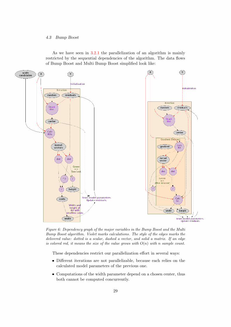
Figure 6: Dependency graph of the major variables in the Bump Boost and the MultiBump Boost algorithm. Violet marks calculations. The style of the edges marks thedelivered value: dotted is a scalar, dashed a vector, and solid a matrix. If an edgeis colored red, it means the size of the value grows with O(n) with n sample count.
These dependencies restrict our parallelization effort in several ways:
� Different iterations are not parallelizable, because each relies on thecalculated model parameters of the previous one.
� Computations of the width parameter depend on a chosen center, thusboth cannot be computed concurrently.
29
4.3 Bump Boost
� The same holds for the width and height in the Multi Bump Boostcase. In Bump Boost the heights could be computed concurrently,and then those parameters of the candidate with the smallest cost areused. On the other hand, the height could also be computed after thewidth being determined, still taking advantage of the precalculatedvalues. Therefore, the edges are green.
We can summarize that the calculations of each iteration as, inside theiteration, of center, width, and height (with a corner case) have to be donein sequential manner.
Thus, the only way to parallelize (Multi) Bump Boost is to do it duringthe calculations of the parameters. As we can learn from the graphs, the val-ues belonging to red edges scale with O(n) with n sample count. Expressionsinvolving these values are problematic for scaling.
We assume that each parallel p = 1, ..., k instance is responsible for somedata, i.e. the continuous indexes Ip = ip, ..., ip+1 − 1 with 1 = i1 < ... <ik+1 = n+ 1. Let us start with Bump Boost:
Center: How a random center can be found is described in 4.3.1. This canbe broken into two steps: First calculating the sum of the squaredresiduals, which can be done efficiently in parallel. The second, find-ing the center is more challenging. Given up =
∑pp′=1
∑i∈Ip r
2i , the
searched value is at worker p with the smallest p for that holds ε ≤ up.At the worker itself, the general search center procedure inside therange Ip can be applied, using a new ε′ = ε − up−1 if p > 1. Also inthe second operation only a fraction of the data needs to be accessed.
Width: By closely examining the sub graph, we identify the computationsuntil the dot products are especially expensive, i.e. they scale withO(n). Ideally, we would like to split those into sub task and indeed wecan:
� Each element of a kernel vector can be calculated independentlyon the other (see equation 20). Thus, the calculation of the wholevector can be parallelized.
� The definition of the dot product for vectors is v·w =∑n
i=1(viwi).This allows us to do each scalar multiplication in parallel andparts of the summation, too. By denoting vn:m as the sub vectorfrom element n to element m of the vector v, we can easily splitthe dot product into m smaller dot products, i.e. sub tasks:
v·w =n∑
i=1
(vi∗wi) =
bn/mc∑
i=1
i∗(m+1)∑
j=i∗m(vj∗wj) =
bn/mc∑
i=1
vi∗m:i∗(m+1)·wi∗m:i∗(m+1)
(26)
30
4.3 Bump Boost
They can be done in parallel and the final value is given by the sumof them.
Height: If the final height is computed in parallel to the widths or after-wards, in both cases the computed dot products in the width calcu-lations can be recycled and the height calculated using a closed-formexpression (see 24, mind that the dot products are already computed).Therefore, we do not need to parallelize here.
Residuals Update: As computing the kernel vector given the computedparameters, this can easily be done in parallel, see equation 25.
As Bump Boost is parallelizable to some extent, also Multi Bump Boostit is:
Center: It is the same algorithm as for Bump Boost.
Width: With the knowledge of the Bump Boost parallelization, all the val-ues of the calculate gradient operation can be computed efficiently (inthe figure the node is called “Calc Gr.”). Given the “height” value,
i.e.k>c,wr
k>c,wkc,w, all the operations we need for the gradient (see 23) are
element-wise subtraction and multiplication completed by a dot prod-uct. This can be done efficiently in two steps by computing the heightas described in the Bump Boost parallelization and after distributingthat value by doing subtractions and multiplications in parallel. Thefinal value then is given by a final parallelized dot product.
Height: For Multi Bump Boost we cannot recycle the intermediate resultsof the width calculation, because the actual width is determined bythe last gradient update. But we can calculate those results again inefficient manner as for the height computation in the previous step.Hence, the height parameter is parallelizable, too.
Residuals Update: It is the same algorithm as for Bump Boost.
After describing the parallelization, we are left with a last problem: thecommunication between the sub tasks assigned to some worker. This isespecially expensive when they are distributed over several hosts. Fortu-nately, this is easily solved by distributing the data beforehand. The only“large”, iteration-persistent variables are X and residuals. By, as assumed,assigning each worker p a slice of the samples and residuals, i.e. XIp andresidualsIp , he can do all the expensive computation locally and just deliverthe result to the master. The master joins the results together to calculatethe actual model parameters. Clearly, the work and data load should asbalanced as possible to reach a good parallelization.
This is categorized as data parallelism (see 3.2.3), because the sameoperations and procedures are carried out on different sub sets of data.
31
4.3 Bump Boost
This parallelization scheme is shown for Bump Boost in the next illus-tration:
Figure 7: This graph illustrates the calculations subdivision onto different workersfor the Bump Boost algorithm. The node border colors orange to red denote dif-ferent work entities, thus those values and computations were stored/executed onthe according workers. Black denotes the master. The edge color green denotes atransfer between master entity and a worker entity. The other graph properties aredescribed in the previous illustration 6.
32
4.3 Bump Boost
Please note, that only the parallelized operations scale with data set sizen, i.e. all the other operations do not depend on n, but on the number ofworkers. This implicates that with increasing data set size the parallelizableparts of the algorithms increase. Therefore, according to the theoreticallaws on scaling (see 3.2.1) Bump Boost and Multi Bump Boost should havebetter scaling properties with larger data sizes. Furthermore, the amount ofdata sent between master and workers as the work load at the master staysconstant with constant number of workers.
Theoretically, these joins may cause a bottleneck. Imagine having n datapoints and n workers. In this case, the master needs to sum up n values andthe approach would not scale. In more detail, in the graph above the meantoperations would be the “join” and additions pointed by the green arrows.Fortunately, all the join and addition operations can be implemented in atree-like structure. In this case, assuming all nodes have the same child-degree C and each worker has C data points to take care of, the asymptoticgrowth would be O(C + logC(n/C)) = O(max(logC(n/C), C)). This is be-cause the operations at the worker nodes grow with C, whereas the joinoperations grow with the height of the tree logC(n/C). More on that in thefollowing paragraph.
How do these versions scale?
As we have seen in 4.3.1, Bump Boost and Multi Bump Boost scaleasymptotically in linear manner. How do the parallelized versions scale?
To investigate that, let us assume that the sample set X of size n canbe split into m partitions of equal size nm. The iteration count is namedI. We start with Bump Boost and treat the number of width candidates asa constant. In the following description, there is one master and m workernodes to compute the algorithm. For simplicity’s sake we do not mentionconstant parts of Bump Boost:
Data fetch: If the workers are distributed and all the data lies at the mas-ter, it takes him O(n) to deliver it to the workers, assuming that noparallelization through different network interface etc. is possible.
If the workers are not on the same machine, i.e. perform on differenthosts, or the data is distributed, f.e. with HDFS (see 6.2.2), it eithertakes linear time to load the data into memory or it is somehow paral-lelized, but the behavior is not predictable. Thus, in worst case eachloads the whole data in parallel.
We can summarize that the fetching the data into memory and todistribute it takes O(n).
Center calculation: The parallel effort, as described above, takes O(nm)for summing up the squared residuals, the work at the master needs
33
4.3 Bump Boost
O(m) for summing up the partial results and is concluded in O(nm)for searching the actual searched value at a single worker: O(nm) +O(m) +O(nm) = O(max(nm,m))
Width calculation: To calculate the kernel vectors it takes O(nm), as itdoes for the sub dot products on the single workers. The finalized dotproduct, i.e. summing up the sub results at the master takes O(m):O(nm) +O(m) = O(max(nm,m))
Height calculation: The height parameter can easily be calculated out ofalready computed dot products, thus takes constant time.
Residuals update: After fetching the computed parameters, this can bedone at the workers in O(nm).
We are left with an overall asymptotic run time with I iterations:
O(n) + I ∗ (O(max(nm,m)) +O(max(nm,m)) +O(1) +O(nm))
= O(n) +O(I ∗max(nm,m))(27)
For Multi Bump Boost the data fetch and the center calculation asthe residual update are the same as for Bump Boost. The width needsto be computed in two steps resulting in O(max(nm,m) + max(nm,m)) =O(max(nm,m)). The height calculation takes O(max(nm,m)), it is basicallythe same effort as a reward calculation in Bump Boost. In this case, theoverall computational cost with I iterations and G gradient descent steps is:
O(n) + I ∗ (O(max(nm,m)) +G ∗O(max(nm,m)) +O(max(nm,m)))
= O(n) +O(I ∗G ∗max(nm,m))(28)
We reach the best performance when nm = m i.e. m =√n holds.
Without the data loading, we improved the asymptotic run time of BumpBoost and Multi Bump Boost from O(n) to O(
√n). As the data loading
needs to be performed only once, the final amortized computational cost isO(max(nm,m)) given I →∞.
Given the case that lots of workers are available, i.e. nm << m, the joinoperations scale worse than the main computations or just to reduce theactual run time, it is possible to do the join operations in a (virtual) treenetwork. This may lead to a smaller run time, if there is lots of data andthe overhead does not overwhelm the run time.
Getting back to the proposal of the tree with C children and each leaf isresponsible for C data points, in which case the join and addition operationstake O(logC(m)) instead of O(m). In the case the asymptotic run time ofBump Boost boils down to:
O(n) +O(I ∗max(logC(m), C)) (29)
34
4.3 Bump Boost
For Multi Bump Boost this results in:
O(n) +O(I ∗G ∗max(logc(m), C)) (30)
Given I → ∞ and taking C as constant, we can say Bump Boost andMulti Bump Boost have an amortized computational cost logarithmic in n:
O(logC(m)) = O(logC(n/C)) = O(log(n)) (31)
35
5 Related Work
5 Related Work
This chapter treats related work in the field of machine learning, to be moreprecise, work that addresses scaling issues.
After the introduction to the popular map-reduce approach in [DG05],[CKL+07] shows how to speedup a variety of machine learning algorithmsusing this simple paradigm. The paper describes how algorithms that fit theStatistical Query model [Kea98] can be rewritten in a certain summationform. Thus by mapping, i.e. calculating the summands, and then reducing,i.e. summing up, the map-reduce approach can be applied. They applytheir principle, among others, to logistic regression, naive Bayes, SVM, ICA,PCA, and neural networks. A similar set of algorithm is implemented in theApache Spark MLlib.
Using a sum to join the in parallel calculated results, Bump Boost andMulti Bump Boost have a similar approach. But the determination of thebump center, for example, is not covered by it. Thus Bump Boost is in somesense too complex for this schema.
While the solution [CKL+07] does not rely on approximation, in machinelearning it is often used for large scale problems. For example, stochasticgradient descent tries to reduce the actual processed data by sampling onthe whole data set. [Bot10] describes how stochastic gradient descent canbe used efficiently, f.e. with averaged stochastic gradient descent or comput-ing second order derivatives, for large scale problems. In [LK12] machinelearning at twitter is described, where f.e. stochastic gradient descent withlogistic regression is used for large amounts of data.
Another example where averaged stochastic gradient descent works wellare neural networks, in this case also named mini batch learning. Thistechnique was successfully applied in [DCM+12] by massively parallelizingdeep neural network learning. Due to its sequential nature, stochastic gra-dient descent is hard to parallelize, [DCM+12] shows how this can be doneby asynchronous updates. More precise, in “Downpour SGD” two clustersparallelize the workload. The data is partitioned onto the entities of onecluster, where each performs the gradient calculations. The gradients thenget pushed to a second cluster, where each host is responsible for a set ofparameters. This cluster is responsible for updating and distributing the ac-tual parameters. A similar approach is used in [LASY14] with a even largersetup.
This idea of a parallel stochastic gradient descent has also been used inseveral works, such as [FS09], to speedup linear SVMs. In contrast to deeplearning, which works well in non-linear settings, non-linear kernels enableSVMs to solve more complex problems [Gar03]. In principle and practiceit is possible to use stochastic gradient descent also with kernels, but thequestion which data points, i.e. support vectors, to prioritize gets prominent[BEWB05, The implementation LaSVM is used in this work.][KSW04]. This
36
5 Related Work
increases the parallelization complexity.SVMs suffer from the complex optimization problem, the more data, the
slower the state-of-the-art SVM solvers. In [SSS08] they claim that moredata should decrease the actual run time when the same prediction errorshould be reached. The idea is, that even though the optimization problemincreases with more data, the actual generalization problem does remain thesame, in contrary should be easier solvable with more data. The authorsgive a theoretical and empirical justification for linear SVMs.
In contrast to stochastic gradient descent, Bump Boost and, in this casemore concerning, Multi Bump Boost optimize the parameters always byusing the whole data set and synchronously.
Another way to parallelize machine learning algorithms is ensemble learn-ing. There are several ways, but the principle is to learn different models ona data set and then combine their single predictions to a global one [MO99].Next to stochastic gradient methods, this is a used technique at twitter forlarge scale problems [LK12]. But it comes with high computational costs, asgenerally each model is trained on the whole data set. In [CBB02] a mixtureof SVMs is proposed to make SVM learning practical, where the output of aset of SVM, each learning on a subset of the data, is combined by a learnedgatekeeper. Even though giving good results, the model is still restrictedby the size of the subsets, i.e. the size of the subset cannot be larger thanpractically manageable by a single SVM. Hence, this approach will not workfor highly complex and large data sets.
Boosting, which is used in Bump Boost, is also a form of ensemble learn-ing as in each iteration a simple prediction function is learned. But thelearning of the bumps is not independent, thus not parallelizable as all theother boosting based approaches.
An interesting solution for large scale learning is given in [RR07]. Theauthors propose to map the actual feature space into a lower dimensionalone and learn on that with fast linear methods. This lower space should bedesigned so that the resulting inner products are approximately the same inboth spaces.
By top-performing in the ImageNet Large Scale Visual Recognition Chal-lenge 2012 (ILSVRC2012) the authors of [KSH12] gave an example on howneural networks can learn features by themselves. The enormous learningtask and parameter space, the net has 69 million parameters and 690.000neurons, is controlled by a highly efficient GPU-implementation and the,back then, new regularization method dropout [HSK+12].
Similar our work also includes a fast GPU-implementation. On the otherhand, Bump Boost and Multi Bump Boost are as SVMs dependent on ameaningful feature space. The kernel methods merely help to predict morecomplex problems. This neural network learns these “meaningful” features,too.
In the introduction, we already mentioned recommender systems. They
37
5 Related Work
relate to our work mainly by the fact that they are a popular Big Dataproblem and application of Apache Spark. The approach of [KBV09] baseson an approximated matrix factorization and is implemented in ApacheSpark MLlib [mll15]. Besides, a proof of concept for Apache Flink is givenin [fli15a] and should be released in future. The actual algorithm is of modestcomplexity, the resulting code [fli15b] in Flink is complicated and, accordingto us, not implementable without an in-depth knowledge of Flink. Indeed[fli15a] mentions that several features were added to Flink to enable thisalgorithm.
38
6 Tools and Frameworks
6 Tools and Frameworks
Before we describe our programs, we would like to introduce the technologythey are based on.
Already well-known and established for GPUs is Cuda and for GPUs andother computing devices OpenCl. Both were used to parallelize programs onsingle devices. Still new are Big Data systems to parallelize computationson computers clusters. In this work we use Apache Spark and Apache Flink.All of them will be described below.
We use the Scipy toolkit to develop a parallelized version of Bump Boostfrom scratch. To accelerate Bump Boost we try to use the libraries CudaMatand PyOpenCl, both have the aim to provide an easy access to Cuda andOpenCl using Python.
Finally, we describe two very popular SVM-solvers: LIBSVM and LaSVM.
6.1 Parallel Computing Device Frameworks
As stated above Cuda and OpenCl were used to parallelize applications onsingle devices. While Cuda’s job is to enable it for Nvidia GPUs, OpenClis more general and helps to port applications on different platforms, fromCPUs over GPUs to FPGAs. Both are data parallel programming languages(see 3.2.3).
Both of them provide a language to program and an application inter-face to (cross-)compile the code and access the devices. The programmingmodel of these languages differs from the common one, because accordingto Flynn’s taxonomy (See 3.2.1), it is build on “Single Instruction Stream,Multiple Data Streams” machines. Common sequential programming mod-els assume “Single Instruction Stream, Single Data Stream” devices. Thisdifferent programming scheme can be a barrier.
To give the reader a broad understanding, let us sketch the following codeexample from an AMD Developer Blog [AMD15]. It is a sample dot-productimplementation in OpenCl:
5 __global const double * x, // i n p u t v e c t o r6 __global const double * y, // i n p u t v e c t o r7 __global double * r, // r e s u l t v e c t o r8 uint n // i n p u t v e c t o r s i z e9 ){
10 uint id = get_global_id (0);
11 uint lcl_id = get_local_id (0);
12 uint grp_id = get_group_id (0);
13 double priv_acc = 0; // a c c umu l a t o r i n p r i v a t ememory
14 __local double lcl_acc[LOCAL_GROUP_XDIM ]; //a c c umu l a t o r s i n l o c a l memory
1516 i f ( id < n ){
17 priv_acc = lcl_acc[lcl_id] = x[id] * y[id]; //m u l t i p l y e l emen t s , s t o r e p r o d u c t
18 }
19 barrier(CLK_LOCAL_MEM_FENCE); // F ind t h e sum o f t h ea c c umu l a t o r s .
2021 uint dist = LOCAL_GROUP_XDIM; // i . e . ,
g e t l o c a l s i z e ( 0 ) ;22 while ( dist > 1 ){
23 dist >>= 1;
24 i f ( lcl_id < dist ){
25 // P r i v a t e memory a c c umu l a t o r a v o i d s e x t r a l o c a lmemory r e a d .
26 priv_acc += lcl_acc[lcl_id + dist];
27 lcl_acc[lcl_id] = priv_acc;
28 }
29 barrier(CLK_LOCAL_MEM_FENCE);
30 }
3132 // S t o r e t h e r e s u l t ( t h e sum f o r t h e l o c a l work
g roup ) .33 i f ( lcl_id == 0 ){
34 r[grp_id] = priv_acc;
35 }
36 }
As hinted above this code gets executed in parallel on different datastreams, and is separated implicitly by the results of the identification func-tions. Again, each thread of this code gets different global and local ids and
40
6.2 Cluster Frameworks
based on them it should access a different data space and thus use a different“data stream”.
In the code above, first all threads multiply in parallel the accordingelements (line 17). Then, by halving the working threads in each round, itsums up the results (line 20 to line 30). This code does it until a small vectorof summands remains, it could be done also until just the final dot-productresult is left over.
The key point we wanted to show, even though the multiplications areeasily done in parallel, for the sum we need to use barriers to synchronize thethreads and we need to take care which thread does which operation. Nextto device-depended characteristics, this programming model makes theseAPIs difficult to handle.
The rest of this section will provide some basic information and referenceson both frameworks.
6.1.1 Cuda
The Nvidia company was the first to offer a general purpose computinginterface for a GPU (see [nvi15]) in 2006. This enabled a new form of GPUusage: using high level languages for sequential parts of the application andaccelerating the parallelizable parts on graphical interfaces. Today, Nvidiaprovides interfaces for several languages such as C, C++ and Fortran.
This new development also had a major impact on scientific research.Besides that toolkits as MATLAB support accelerations by GPU usage now([mat15a]), high end performance gets reached for example in the neural net-work research. To name one example: the successful convolutional network([ale15]) of Alex Krizhevsky at the ImageNet([KSH12]).
6.1.2 OpenCl
OpenCl is a project of the Khronos Group (see [ope15a]). Whereas Cuda isonly available on Nvidia GPUs, Khronos advertises OpenCl as “first open,royalty-free standard for cross-platform, parallel programming”[ope15a]. Allmajor vendors implement the standard in some way. To name some: Intel,AMD, Xilinx, Altera, ARM, IBM, and Nvidia.
Although this variety of vendors and thus devices providing an OpenClinterface, CUDA still seems to be more popular. F.e. MATLAB does notprovide accelerations support by OpenCl devices [mat15b]. A cause maybeis the late following up in the year 2009 [ope15b].
6.2 Cluster Frameworks
A completely different idea compared to Cuda and OpenCl are Spark andFlink. Instead of accelerating the computation as much as possible on a sin-gle device, their first goal is to make the computation possible, because of the
41
6.2 Cluster Frameworks
large data that has to be processed. And second to reduce the computationtime by parallelizing the effort on a computer cluster.
As introduction, we describe the Apache Big Data stack they are partof. This includes a short development history, including its first successfulproject Hadoop. In the end we describe Spark and Flink.
6.2.1 Apache Big Data Stack
1 Computer clusters, large amounts of data, and distributed programs arefor a long time part of computer science. But before the rise of the ApacheBig Data stack, these challenges were mostly solved with high end hardwareand software systems. The software that is merged into that described stack,especially the most important one, Apache Hadoop, changed the access toBig Data solutions.
We named in this case the Apache Big Data stack, because it is thepredominant software bundle for Big Data applications. Notably all thissoftware is open source. To the best of our knowledge, no major softwarevendor has yet presented a more evolved solution yet.
The following diagram depicts the Apache Big Data stack:
1Great part of the information of this section are summarized from [KFLQ].
42
6.2 Cluster Frameworks
Figure 8: The Apache Big Data stack. Apache Flink is missing and would be in thesame place as Apache Spark. (Year 2013. From: [KFLQ])
“Having specialized hardware like Super Computing infrastructures fordoing such processing is not economically feasible most of the time. Largeclusters of commodity hardware are a good economical alternative ...” [KFLQ].This leads to new challenges such as hardware heterogeneity, node manage-ment, and common and expected hardware failures. These were tackledby Apache Yarn and Mesos. Both’s application purpose is to manage theresources in a cluster.
The next problem is providing the data inside the cluster. Hadoop FileSystem (HDFS) solves this problem in the Apache Big Data stack.
43
6.2 Cluster Frameworks
The last, general problem is how to distribute the actual work. HereSpark and Flink come into the game, next to several other applications.
Still notably for us are the data analytic tools Mahout and MLlib. Bothof them provide popular machine learning algorithms on top of Spark and/orHadoop. They have a very similar set of algorithms. To us, MLlib seemeda bit more advanced, therefore we have chosen it as example in our experi-ments.
6.2.2 Hadoop, HDFS, and YARN
Now we introduce the core pieces of the Apache Big Data stack. NamelyHadoop (version 1.0 released in 2011, version 2.0 in 2013 [apa15c]) with theidea of MapReduce and it’s components HDFS [apa15b] and YARN [apa15e].
New to Hadoop was the simplicity and the short development cycles fordevelopers: “Performing computation on large volumes of data has beendone before, usually in a distributed setting. What makes Hadoop uniqueis its simplified programming model which allows the user to quickly writeand test distributed systems, and its efficient, automatic distribution of dataand work across machines and in turn utilizing the underlying parallelismof the CPU cores.” [had15] The simplified programming model is the Map-Reduce-approach. The automatic distributions of data and work is done byHDFS and YARN.
Yahoo initially developed Hadoop based on the Google File System[GGL03] and the famous Map-Reduce-approach [DG08] [KFLQ]. After mak-ing it open source it became a great success and the corner stone for theApache Big Data stack.
Map-Reduce-algorithms base on a tuple of functions: a function mappingfrom A to B f(A) : B and a reducing function f(B,B) : B. Thus, they areeasily distributable. For example v · v> can be expressed with: the mappingf(xi) = xi ∗ xi and the reducing function f(xi, xj) = xi + xj . The factthat the developer just needs to provide these functions is one case for thesimplicity, because f.e. there is no need to concern about marshaling dataor inter process communication. Another reason is, that the system itself isnot the fastest, but it is designed for flat scalability [had15]. This means noneed to refactor or rewrite the program if the developer wants to increasethe number of cluster nodes.
A very important characteristic of the distribution strategy is the ap-proach of moving computations to the data instead of vice versa.
This simple yet quite powerful programming model suffices for varietyof tasks, but for some algorithms it is often not enough, especially machinelearning ones.
The very base of Hadoop is the “Hadoop File System” (HDFS). It isdesigned for large files, which usually are once written and then often read.These large files are split into chunks and those are distributed with some
44
6.2 Cluster Frameworks
replication factor onto the cluster. The file system interface is similar to theLinux one.
In the first version, YARN did not exist and the functionality was in-tegrated into MapReduce. From Version 2 on they were split and YARNgot a fundamental base for other projects. YARN basically offers to reservecluster resources for an application and uses those to execute the applicationprocesses. There is no failure handling included. Thus, this is left to theapplication developer.
6.2.3 Spark and MLlib
To overcome the Map-Reduce restrictions the Spark [ZCF+10][apa15d] pro-gram was created. Version 1.0 was released in May 2014 [spa15a]. Theprogramming model of Spark is based on a “resilient distributed dataset(RDD), which is a fault-tolerant collection of elements that can be operatedon in parallel.” [spa15d] Thus, it distributes large datasets in the memoryof the cluster and computes operations in parallel, if possible.
The usage of Spark is as follows: Spark provides a client library thatcommunicates with a cluster or a standalone version. A program using thislibrary is called master. Inside this program, RDDs can be used and all theoperations on those are dispatched to the cluster. To enable optimizationsand reduce traffic, those operations are just scheduled when the master wantsto retrieve a result of an RDD operation.
As for Hadoop, the user does not need to concern about the distributionof the data or computation and therefore Spark scales flat too.
The most important operations provided by RDD’s are:
map: Mapping the set to another.
filter: Filter elements according to the binary value of some function.
union: Union two sets.
intersection: Interset two sets.
join: Join elements with the same key.
reduce: Reduce all elements to one result element.
The RDD sets usually are not sorted and there is no random access, thusthe operations are very similar to mathematical operations of sets.
On top of Spark, MLlib [spa15c] was developed. Next to some generalmath features it provides several stochastic gradient descent algorithms.To name some: linear SVMs, logistic regression, decision trees, k-meansclustering, principal component analysis.
45
6.3 Python
6.2.4 Flink
This project [apa15a] was created at the TU Berlin under the name Strato-sphere [ABE+14]. After the admission as project in the Apache SoftwareFoundation it was renamed to Flink due to naming conflicts. During thework on this paper, it was still in the incubating phase.
From the first point of view it provides a very similar functionality asSpark, i.e. the distributed manipulation of sets. In fact, nearly the samecode semantics belonging to set operations work for both frameworks, butunder the hood they are quite different. While Spark programs are executedas master and communicate with a cluster, Flink programs are submitted toa server, which executes them on a cluster. And whereas the Spark programmanipulates sets, a Flink program creates a dataflow execution plan. Thismeans, the developer specifies the set sources, the manipulations on themand the sinks, where to store them. Then the server creates out of that plana real program and executes it on the cluster.
This restricts the programmer to use only operations supported by Flink,whereas in Spark he can fall back to general purpose computations on itsmaster. On the other hand, it allows the Flink compiler to optimize the planand further to create a pipeline structure, through which the data passes.Thus, those programs can also be used for stream processing [ABE+14].
We will discuss the further implications of the Flink programming modellater in this work.
6.3 Python
In this two final sections, we describe more common tools. We begin with ashort introduction into our chosen python projects.
6.3.1 Scipy, Numpy, Matplotlib
The python project for scientific tasks called Scipy (see [sci15]) got popularin the last years, due to the flexibility of Python and the great work ofthe community. We mostly use the Numpy (see [num15]) module whichprovides a n-dimensional array object backed by fast C-implementationsand other useful mathematical features, such as linear algebra or randomnumber functions.
Related to the popular MATLAB plotting functions, Matplotlib (see[mat15c]) provides a very powerful plotting library in Python. We use it toanalyze and visualize our results.
6.3.2 CudaMat
The module CudaMat (see [Mni09]) created by Volodymyr Mnih is a simpleyet powerful library to do matrix computations on CUDA-enabled devices.
46
6.4 SVM Programs
It is aligned to Numpy arrays and provides conversion functions betweenthese types. There is no open interface to compile CUDA code.
6.3.3 PyOpenCl
PyOpenCl does a somewhat different job. Similar to CudaMat it enables ac-celeration on GPU-devices and provides some basic support for one-dimensionalarrays. But the main scope is to provide an easy way to create and compileOpenCl code. For this purpose, it can abstract several OpenCl managementtasks, especially memory management.
This project was created by Andreas Klockner (see [pyo15]), who alsomaintains a similar module named PyCuda (see [pyc15]).
6.4 SVM Programs
Now we would like to conclude by presenting two popular SVM-solvers. Forthe general SVM-Algorithm please consider 4.2.
Both of them use the popular LIBSVM/SVM-light file format [las15].Because of it’s popularity and to have the same starting point for all algo-rithms, we use it for the Bump Boost implementations, too.
6.4.1 LIBSVM
The first solver is called LIBSVM (see [CL11]), now in its third version (see[lib15a]). This library supports, next to support vector classification, alsoregression and distribution estimation. The implementation is a SMO-likealgorithm described in [FCL05]. According to [CL11, page 26] the computa-tional cost of this algorithm is in the worst case (all cache misses) O(I ∗n∗d)with I iterations, n data samples of d dimensions. Unfortunately, “empiri-cally, it is known that the number of iterations may be higher than linearto the number of training data.” [CL11, page 26]
6.4.2 LaSVM
The second one is called LaSVM (see [BEWB05]) and uses an approximateonline learning approach, which delivers already a good result after a singlepass on the data. Even though some parts have “asymptotic cost ... liken2 at most.” [BEWB05, page 10], the final algorithm has runtime of “n3
behavior of standard SVM solvers.” [BEWB05, page 10] The developersclaim to use considerably less memory than LIBSVM [las15].
47
7 Implementations
7 Implementations
This chapter describes the various implementations of the Bump Boost al-gorithm. The aim is to give the reader a good understanding of how thecode base works and further how different computing framework influencethe development. Of special interest is the usage of the Spark and Flinkframework, which we describe and compare in more detail. The final subchapter gives an informal impression on some coding fragments .
7.1 General Framework
Caused by the usage of different frameworks and technologies as by thelengthy and numerous runs it was necessary to create a general framework.The main purposes of this framework are:
Installation: An easy installation of all components, programs and datasetson the given computer.
Single interface: Providing a single interface for all algorithms and imple-mentations to enable comparable tests and runtime measurements.
Testing: The functionality of the algorithms should be ensured by auto-matic tests.
Automatizing: The experiments with all their different implementations,configurations and datasets as their repetitions need to be scheduledand supervised automatically.
Analysis: To get a quick overview, the automatic creation of plots andtables is useful. For further understanding, an interface to customizethe plots is, too.
In order to achieve these goals the following technologies were chosen.GNU Make (see [gnu15]) for the installation process, for all the rest we relyon Python and the marvelous Scipy environment with Numpy, Nosetests,and the Matplotlib (see [sci15]).
To achieve our goals the following design was used:
Installation: Using GNU Make all the needed libraries and datasets weredownloaded, compiled, created, and installed automatically.
Single Interface: A python class hierarchy provides a single interface forthe test and experiment procedures. All the implementations use thisinterface. For those not using Python, the implementation of thisinterface is more a stub, which converts the input, output data andlaunches the according programs.
48
7.2 Java
Testing: With Nosetests all the algorithms were tested. This is especiallyuseful for Bump Boost as we are using various implementations andwould like to ensure that all work in the complete same way.
Automatizing: Different self-made Python-programs allow us to declareand launch experiments by specifying the configured implementations,datasets, repetitions etc. For each run the runtime and test perfor-mance is measured.
Analysis: For each experiment the framework is able to automatically cre-ate the most important plots. For more enhanced analysis tasks, aninterface for an enhanced plotting is provided.
7.2 Java
This code was originally written by Mikio Braun and is used for the eval-uation in [BK]. The obtained code was not runnable, thus different fixeswere needed to get it back to work. This affected mainly input and outputmechanisms. At this point, we would like to emphasize that nothing of thealgorithm implementation itself was changed, except some minor changesdescribed below. Therefore, the run time should be comparable to the onein [BK].
For the framework alignment we added different configuration parame-ters. They allow us to change each control argument and to get completesame behavior as for the other version.
Achieving this, a small change has been introduced in the procedure forchoosing the bump center. In the original implementation the first value ofthe sample array could not been drawn and the last one’s probability wasincreased by the one of the first sample. All in all, this does not influencethe effectiveness of the program much, we have changed to get the samebehavior as in the other versions.
In the end we point out the particular characteristics of this version.First of two it uses the double data type, i.e. 64-Bit floating point numbers,whereas the other versions use the float data type, i.e. 32-Bit floating pointnumbers. The consequence is a slower program and the use of memory forsamples etc. doubles. Second, this version uses JBlas ([jbl15]), whereasother implementations might use other linear algebra backends.
7.3 Python
The language of our choice is Python. Next to the scripting capabilities,useful for the general framework, Python’s Scipy offers a fast and advancedtoolkit for scientific and mathematical computations. Besides this core, nu-merous libraries provide interfaces to other technologies, f.e. CudaMat forGPU-enabled computations (See 6.3).
49
7.3 Python
All the following programs implement the above presented interface.Thus, the algorithm gets executed in the same process as the experimentscheduler. Other external implementations get invoked in an own one. Thisshould have negligible influence on the runtime.
Below, we describe the characteristics of the various implementations.
7.3.1 Development Version
This initial version is just used for development reasons. It provides a fullyfunctional and correct implementation of Bump Boost and is therefore usedas reference point in the tests and further development. Besides the cor-rectness, it is up to the order of a magnitude slower than the other pythonversions. Therefore it is not used in the final experiments.
7.3.2 Parallelized Version
Based on the theoretically best parallelization of Bump Boost (see 4.3.3)two interfaces were created. The basic work flow between them is sketchedhere:
50
7.3 Python
BumpBoost Iterations
UCC
Initialize Data
Get Bump Center
Get Bump Width & Height
Update Residuals
Get Bump Center
Get Bump Width & Height
Update Residuals
Teardown
LCC
Initialize Data
Get Residual Sum
Search Center
Get Dot Products
Update Residuals
Get Residual Sum
Search Center
Get Dot Products
Update Residuals
Teardown
Figure 9: UML Sequence Diagram with basic work flow for two iterations betweenthe algorithm implementation, the UCC, and the LCC in the Bump Boost case. Forfurther descriptions, see below.
51
7.3 Python
The first one, named “Upper Computing Core” (in the following UCC),mainly abstracts the calculation of the various parameters in a single iter-ation. Next to that, functions to setup and tear down the component asupdate the residuals are provided.
The second one is named “Lower Computing Core” (in the followingLCC). The LCC is designed to represent the leaves and nodes inside thecomputing tree i.e. the distributed computation parts. While the workof the UCC is still done at master node, work of the LCC can be donedistributed and remotely.
To describe the processes in more detail:
Center Search: the LCC calculates the sum of the squared residuals, theUCC then chooses the random element and finally it is left to the LCCto find it.
Bump Boost Width and Height: to calculate the height and width inthe Bump Boost case the LCC calculates the needed dot products andthe UCC computes out of them the costs and the final height.
Multi Bump Boost Width and Height: in the Multi Bump Boost caseit is a bit more complicated. In the UCC the gradient descent stepswere done, the LCC mainly helps to complete them by first calcu-lating the dot products for the needed height and then finishing thegradient calculations (taken from the file “python/implementation-s/numpy bbcc” inside the code repository, see appendix B):
52
7.3 Python
1 # Here h o l d s : a c t u a l w i d t h = 10** w id th2 def get_gradient(width):
3 kv_dot_kv , kv_dot_u = lcc.
compute_first_dot_products(center , width)
45 height = 0
6 i f kv_dot_kv != 0:
7 height = kv_dot_u / kv_dot_kv
89 grad_width = 2 * height * lcc.
compute_second_dot_products(center , width ,
height)
10 return grad_width
1112 # Do g r a d i e n t d e s c e n t13 ...
1415 for i in range(self._gradient_descent_iterations):16 grad_width = get_gradient(width)
17 # . . .18 width = ...
1920 # Ca l c u l a t e f i n a l h e i g h t21 kv_dot_kv , kv_dot_u = self._lcc.
compute_first_dot_products(center , width)
22 height = 0
23 i f kv_dot_kv != 0:
24 height = kv_dot_u / kv_dot_kv
2526 width = 10** width
Where the UCC is implemented only once using numpy, the LCC is thecomputation intensive part and thus realized in different versions. They aredescribed below.
7.3.3 Parallel and Remote LCC
The parallel LCC creates just n Python-threads and distributes the work tothem. In addition to forwarding the calls and arguments, this core splits thework i.e. arguments apart and joins the results meaningful together. ThisLCC would be an inner node in the tree description of the Bump Boostparallelization (see 4.3.3).
The remote LCC is in fact just a stub, which forwards the call andargument to a remote server. A simple but powerful idea. In the treedescription of the Bump Boost parallelization, this one is not visible as itjust forwards data.
53
7.3 Python
As Python does not support real threads because of the Global Inter-preter Lock (see [pyt15]), we use a more general approach by first splittingthe work using the parallel LCC and then forwarding it using the remoteLCC. These remote points, each an own process, can be either on the localor on a remote host. In the local case, this is an easy way for IPC usingPython. In the remote one, it is an easy and powerful way to parallelizeBump Boost on different hosts.
The following graph shows an example structure. At the top is the UCCcontrolling the root LCC. A parallel LCC splits the data flow to its children.While a remote LCC just forwards the data. The leafs then do the actualcomputation, besides the merging in the parallel LCC:
Figure 10: An example tree of LCCs.
7.3.4 Numpy LCC
The easiest implementation is this one. Using the Numpy toolkit, it imple-ments the interface in a few lines of code, but is still highly effective.
7.3.5 CudaMat LCC
It uses the CudaMat project described in 6.3.2.One of CudaMat’s benefits is the easy and Numpy-like interface. Thus,
porting code written in Numpy to the CudaMat library is quite easy. As-suming all the functionality is available.
In our implementation this is not the case, caused by a missing cumu-lative sum procedure used in the center search operation. Therefore, weused the alternative approach doing some sort of binary search (see 4.3.1).Even though much more data needs to be accessed, the performance penaltyshould be modest thanks to the massive parallel characteristics of GPUs.
54
7.4 Big Data Frameworks
7.3.6 PyOpenCL LCC
Unfortunately, we were not able to control the complexity of the OpenClframework and create a performance boost. Therefore even having a workingimplementation, we refused to use it for the experiments.
Here we would like to describe in a short way the main advantage ofPyOpenCl (see 6.3.3) and our problems. The benefit of working with OpenClis that, the code can be used in a parallelized way on different computingdevices i.e. CPU and GPU. On the CPU, the code is parallelized on differentcores by the OpenCl framework. Another benefit is that OpenCl code canrun on ATI, Intel and Nvidia GPU-devices, whereas Cuda code can only runon Nvidia GPU’s. Next to this benefits inherited from OpenCl, PyOpenClprovides a neat library with a lot of abstractions for memory management,compilation processes etc. and a vector class with fast operations.
So far so good, on the other hand the OpenCl computing model can betricky and for different devices different options behave in different ways.Without specific knowledge it is hard to get working code and especiallya performance boost (For an example see 6.1.). A drawback of PyOpenClitself is the missing support for matrices. F.e. CudaMat supports it. InPyOpenCl, all operations that can not be done on a flatten array need tobe implemented in OpenCl code.
7.4 Big Data Frameworks
One of the initial objectives of this thesis was the examination of the BigData frameworks Spark and Flink and their applicability for implementingmachine learning algorithms. Whereas in the previous descriptions we leftout most coding details, in this sub chapter we want to describe it in moredetail.
In the chapter 6.2 we already described in the general environmentaround and the idea behind those frameworks. Now we would like to dothe next step and describe the impact of these models on our work flow.This is done by first describing the implementation effort for Spark andFlink. In the next sub chapter a specific code section is compared.
Please note that only a simplified subset of the code is shown here, for thewhole and working Scala-code please see the code base referred in appendixB.
7.4.1 Spark
The Spark (see 6.2.3) way is a very pragmatic one. The main idea of Sparkis to have a “resilient distributed dataset“ called RDD and to make transfor-mations to it. All of them get cached until the result is explicitly requested.That’s the only impact on the programming structure. This means, thedeveloper can program as he would like to, especially in cases where the
55
7.4 Big Data Frameworks
framework does not solve the problem well, he can fall back to, in our case,Scala.
On the other hand, this restricts the possibility of Spark to optimize thecode and increases the impact of the developer on the program efficiency.
As we already stated, for Spark exists the machine learning library ML-LIB. We decided not to use it, because it did not seem very promising, inother words evolved. One of the reasons was the missing dot product be-tween matrices and vectors which is needed in Multi Bump Boost. Theother was that for Flink no such library exists, but for comparisons sake wewanted to keep the code as similar as possible.
The solution to our own math library was subclassing the Spark RDDclass in combination with Scala implicits [OSV08, See sub chapter 6.12].This allowed us to code more easily. In the rest of the section we describeour design choices.
Each of our RDD’s represents a matrix of shape n x d, thus possibly ofshape n x 1, and each element of the set represents a row of that matrix. Dueto the missing ordering in a set, each element consists of a row index and anarray containing the row elements. The same design choice was made by thecreators of the MLLIB (see [spa15b]). As a consequence, for each operationincluding two matrices or vectors they need to be “zipped” together i.e. theelements need to be joined by index. This can be a major impact on theperformance during math operations, especially if the according elementsare not stored on the same hosts.
In the listing we show the simplified code for element-wise math opera-tions:
Given two vector RDDs, first the row elements are “zipped” togetherand then the according operations are applied on the single vectors(line 2-5). As stated, this means that the elements are joined by their row indexes.In Spark joins require a RDDs with elements of the form (key, value) andreturn a RDD with elements of the form (key, (value1, value2)). Knowing
56
7.4 Big Data Frameworks
this, we can follow the flow, where in line 10 the vector RDDs were mappedto the required form using keyfy (line 11) and then joined together. Wedon’t need the key, so the mapping in line 10 removes it.
The actual operations on the vector are a loop over the array elementsperforming the desired operation.
Thanks to the flexibility of Scala we can overload operators such as “+”,“-” etc. and thus create a quite readable code. F.e. in the next listing,two vector RDDs can be element-wise multiplied just by writing “X1 * X2”,which invokes the operation in line 4 above.
7 X1.fold(Vector.maxValue(dimensions))({(acc , element)=>acc min element })
8 def maxV(X1: RDD[Vector], dimensions: Int) =
9 X1.fold(Vector.minValue(dimensions))({(acc , element)=>acc max element })
10 ...
11 }
The code above illustrates how three of the basic operation types, namely“map”, “reduce”, and “fold”, work.
Line 3 shows a mapping of a vector RDD to the a vector RDD with it’sabsolute values.
In 6.2.2 we already described how reduce functions work. Here, wepresent an actual example. In the lines 4-5, first the vector RDDs get mul-tiplied element-wise (see previous listing) and then the rows are summedup using the reduce function of the RDD class, resulting in a vector ormatrix-with-vector dot-product.
While the reduce operations can be performed in parallel, the fold oper-ations can not. Given an initial accumulator element a, for all elements ei ina set following update operation is performed: a = f(a, ei). In our case, thissemantic is used for a minimum and maximum function. After initializingthe fold operation in line 7 with the maximum possible value the minimumis found with a function that always returns the smaller element. In line 8it is done vice versa for the maximum.
If the result is a single element, f.e. using fold or reduce procedures,Spark returns the value instead of dataset with one element. Contrary toFlink as we will see later.
Backed by this mathematical functionality implementing Bump Boostand Multi Bump Boost was not a big deal as we could rely on Scala’s power.
57
7.4 Big Data Frameworks
For searching the bump center we make the same design choice as inGPU case (see 7.3.5) and do some sort of binary search (see 4.3.1), but thereasons differ. Whereas in the GPU case we could not make a cumulativesum and thus we took advantage of the GPU parallel architecture, in Sparkwe could do it by fetching each element/row of a vector/matrix. The resultwould be really slow as it includes n transfers from the nodes to the masterof a single element. We are faster to make only log n transfers, even thoughwe might sum up up to the half of the elements in the vector at the nodes.
7.4.2 Flink
The Flink way is the idealistic one. Flink(see 6.2.4) programs base on a dataflow model built around data sets. This restricts the power of the developeron one hand, on the other the compiler has much more control, thus ispotentially able to optimize the program better than f.e. in the Spark case.
Spark can be seen as a feature to a general purpose language. Flinkprograms are not general purpose. A general purpose language s.a. Scala isused to describe a Flink-program, but the Flink program itself is tied to thedata flow paradigm.
For Flink, a math or machine learning library does not yet exist (aMahout implementation is planned [mah15]). Fortunately, due to the similarsemantics, we can use most of the code from Spark, with all its benefits anddrawbacks. The only bigger difference is that we can join the rows/elementsof matrix/vector more easily by addressing their elements:
One of the major drawbacks of Flink is that everything is a data set.In Spark, the result of a dot product is a vector, in Flink, it is a data setwith a single vector. If we would like to subtract a single vector from allvectors in a data set, this vector is a single one in a data set. In this case,either a cross join needs to be performed or a special annotation operationcalled “withBroadcastSet” needs to be applied. This broadcasts the passeddata set (line 10) to all executing nodes, where it is converted into a Scalacollection and extracted into a member object(line 7). Finally, in the mapfunction the actual subtraction is applied:
7 v = getRuntimeContext.getBroadcastVariable("v").toList.head
8 }
9 def map(x: Vector) = {x - v}
10 }).withBroadcastSet(X2, "v")
11 ...
12 }
A more realistic example is given in the next listing. It shows the finalupdate of the R-Prop algorithm (see 4.1.4) i.e. width = width + update ∗sign(gradient). As everything is a data set, also the values for the updateand gradient variable are data sets, thus need to be broadcasted into themapping function of the data set:
This is already quite cumbersome for such simple operations. Further-more, Flink does not offer control statements for operations on data sets.
59
7.4 Big Data Frameworks
In more detail, the content of data sets can be added, modified, and re-moved, but if a certain operation is applied to a data set or not is fixed[fli15d]. Imagine a pipeline structure which controls the passed content, butthe structure itself cannot be modified. An example of the code explosionis given in the next section 7.5.2.
This workaround of using data sets with single values, broadcasting datasets and putting the program logic into “open” function of these rich mapand filter functions make Flink quite flexible. But the programming is hardand the compiler has problems with the increased amount of nodes, i.e. datasets, the program contains. More on that below.
Other restrictions are imposed when using loops. Flink offers two typesof loops. The first one is called “Bulk Iteration”, which allows to modify adata set with an iteration function for n times. The second one is called“Delta Iteration”, which allows to provide a work data set and cumulatesthe results in a solution set. The loop performs until the work set is emptyor the developer set maximum iteration count is reached. For both, also acustom “aggregator” can be used to control the termination (see [fli15c]).
The following example shows how bulk iterations work by calculatingthe factorial of 100. First of all, an iteration needs a working set, i.e. aset used for the iteration, created in line 1. Line 3 states that we wantto make 100 iterations. What each iteration does, is determined by the socalled step function, line 4 to line 8, which gets as input in the first roundthe input data set, in our case “initial”, then in each round the output ofthe last iteration. Please note that Scala functions implicitly return the lastobject in a function, in this case “result” in line 8. In lines 4-7 the input data“iterationInput” gets mapped to the “result” data set. In the map functionthe factorial gets calculated by multiplying the only number in the data setwith“getIterationRuntimeContext.getSuperstepNumber”, which returns thecurrent iteration index beginning at 1. As mentioned above, everything is adata set, thus to update the factorial value we need to use a mapping.
1 val initial = env.fromElements (1)
23 val factorial = initial.iterate (100) {
4 iterationInput: DataSet[Int] =>5 val result = iterationInput.map { i =>6 i * getIterationRuntimeContext.getSuperstepNumber
7 }
8 result
9 }
60
7.4 Big Data Frameworks
The first problem using these iterations is that only one variable, i.e.changed during one iteration, data set can be passed into the loop, abovecalled working set. This results in strange workarounds. An example isthe following loop in the R-Prop algorithm. First, all needed variables, i.e.actual width, update value, and last gradient, need to be merged into oneset, and then in each iteration they need to be separated at the beginning(line 12-14) and merged in the end (line 18-22):
1 ...
2 val startWidth = env.fromCollection[Vector ](Seq(startWidthVector))
3 map {x => new Vector(0, x.values)}
4 val startUpdate = env.fromCollection[Vector ](Seq(startUpdateVector))
5 map {x => new Vector(1, x.values)}
6 val startLastGradient = env.fromCollection[Vector ](Seq(zerosVector))
7 map {x => new Vector(2, x.values)}
89 var stepSet = startWidth union startUpdate union startLastGradient
13 var update = stepSet filter {_.id == 1} neutralize;
14 var lastGradient = stepSet filter {_.id == 2} neutralize;
1516 ...
1718 width = width map {x => new Vector(0, x.values)}
19 update = update map {x => new Vector(1, x.values)}
20 lastGradient = lastGradient map {x => new Vector(2, x.values)}
2122 width union update union lastGradient
23 }
24 val width = stepSet filter {_.id == 0}
25 ...
In addition, it is not supported to nest loops, nor will it be in the nearfuture [fli15j]. Thus it’s hardly possible to implement Bump Boost and MultiBump Boost. Unfortunately, we discovered this during the development,because the fact has not been stated in the official documentation(Not in[fli15c] nor in [fli15d] as of Flink version 0.8, January 26. 2015).
During the implementation of Bump Boost and Multi Bump Boost we en-countered several bugs ([fli15e], [fli15f], [fli15g], [fli15h], [fli15i]) which neededto be fixed by the Flink developers. Even though Flink is still under devel-opment, some of the bugs were of general nature. Because of this and aftersome discussions with the Flink developers, we have the impression thatnobody tried to implement something similar in Flink before.
61
7.5 Selected Code Comparisons
In the end, we were not able to produce a working Bump Boost or MultiBump Boost program using Flink. After completing the implementation fora single iteration, which worked fine for both algorithms, we would haveneeded a nested loop to repeat that iteration. Unfortunately, this is notsupported by Flink.
We tried to replicate the loop code using a template script. It waspossible to do two iterations. Doing the step from two to three iterationsthe Flink server did not stop computing. We suspect that the compilercould not cope with the complex computation graph, because each variableis a data set and Flink tries to optimize the flow of them all, not knowingthat only one element per time will be inside each of these data sets and nooptimization is needed.
To summarize, the biggest problems using Flink are a missing linear al-gebra library and the restrictions of unordered sets when creating an efficientmatrix implementation as it is for Spark. Furthermore, the loop semanticsand the mantra “everything is a data set” make the coding cumbersome andhard. Even more, not all algorithms can be expressed in Flink as BumpBoost and Multi Bump Boost show.
Due to all these problems, it was not possible to implement and testBump Boost and Multi Bump Boost on the Flink framework. An exampleof how complex Flink code can be compared to Spark code is given in thenext section.
7.5 Selected Code Comparisons
In this final section we compare some code fragments of selected implemen-tations we discussed above. The scope of this is to introduce the reader tothe code complexity depending on the language and platform choice, not tointroduce the reader to language, platform, or code details.
We begin with the code to draw a center according to the given distribu-tion comparing the implementations in Numpy and CudaMat. We concludeby illustrating an impression of the code for R-Prop in Multi Bump Boostusing Spark and Flink.
For the whole and working code please see the code base referred inappendix B.
7.5.1 Draw Center
The probability distribution and the algorithm, how to determine a center inBump Boost and Multi Bump Boost are outlined here 4.3.1. Two differentversions are named. One is using a cumulative sum, the other a binary searchapproach. The former is implemented in the left listing using Numpy. Thelater is used in the right one using CudaMat, because a cumulative sum isnot supported:
62
7.5 Selected Code Comparisons
1 ...
2 # common code3 def get_center(self):
4 s = self._lcc.sum_u_2 ()
5 x = s * numpy.random.rand (1).
astype(self._data_type)[0]
6 c = self._lcc.search_center(x)
7 return c
8 ...
9 def sum_u_2(self):
10 self._u_cumsum = (self._u**2).
cumsum ()
11 return self._u_cumsum [-1]
1213 # r e t u r n s c e n t e r wh ich b e l o n g s to t h i s
random s t a t e14 def search_center(self , x):
15 ret = self._X[numpy.sum(x > self.
_u_cumsum)]
16 self._u_cumsum = None
17 return ret
18 ...
1 ...
2 # common code3 def get_center(self):
4 s = self._lcc.sum_u_2 ()
5 x = s * numpy.random.rand (1).
astype(self._data_type)[0]
6 c = self._lcc.search_center(x)
7 return c
8 ...
9 def sum_u_2(self):
10 self._u_2 = cudamat.empty(self._u.
shape)
11 self._u.mult(self._u , target=self.
_u_2)
12 return self._u_2.sum(0).sum(1).
asarray ()[0, 0]
1314 # r e t u r n s c e n t e r wh ich b e l o n g s to t h i s
random s t a t e15 def search_center(self , x):
16 r = [0, self._X.shape [0]]
17 while r[1]-r[0] > 1:
18 middle = int (math.ceil((r[0]+r[1]) /2.0))
1920 rs = self._u_2.get_row_slice(r
[0], middle)
21 s = rs.sum(0).sum(1).asarray ()
[0, 0]
22 self._free(rs)
23 i f x > s:
24 x -= s
25 r[0] = middle
26 e l se :27 r[1] = middle
2829 ret = self._X.numpy_array[r[0]]
30 self._u_2 = self._free(self._u_2)
31 return ret
32 ...
For a general understanding, the “get center” function draws the actualcenter,“sum u 2”computes the sum of the squared residuals and“search center”retrieves the actual center value.
63
7.5 Selected Code Comparisons
7.5.2 R-Prop
This gradient descent algorithm is described here 4.1.4. It is used in MultiBump Boost to calculate the width parameter. The width is boxed into therange minWidth < width < maxWidth. We would like to leave the readerwith a general impression, thus do not further explain the coding details.
While in Flink the code is much longer due to the above stated problems:
1 . . .2 def calcMBBWidth( env : ExecutionEnvironment , centerX : DataSet [ Vector ] , r e s i d u a l : DataSet [ Vector
] , c en t e r : DataSet [ Vector ] ) : ( DataSet [ Vector ] , DataSet [ Vector ] ) = {3 val startWidth = env . f r omCo l l e c t i on [ Vector ] ( Seq ( Vector . ones ( c on f i g . d imensions ) * c on f i g .
startWidth ) ) map {x => new Vector (0 , x . va lue s ) }4 val startUpdate = env . f r omCo l l e c t i on [ Vector ] ( Seq ( Vector . ones ( c on f i g . dimensions ) * 0 .01F) )
map {x => new Vector (1 , x . va lue s ) }5 val s ta r tLas tGrad i ent = env . f r omCo l l e c t i on [ Vector ] ( Seq ( Vector . z e r o s ( c on f i g . d imensions ) ) ) map
{x => new Vector (2 , x . va lue s ) }67 var s t epSet = startWidth union startUpdate union s ta r tLas tGrad i ent8 s tepSet = stepSet . i t e r a t e ( c on f i g . g r ad i en tDe s c en t I t e r a t i on s ) {9 s tepSet =>
10 var width = stepSet f i l t e r { . id == 0} n eu t r a l i z e ;11 var update = stepSet f i l t e r { . id == 1} n eu t r a l i z e ;12 var l a s tGrad i en t = stepSet f i l t e r { . id == 2} n eu t r a l i z e ;1314 val grad i en t = getGradient ( centerX , r e s i dua l , center , width ) // n e u t r a l i z e15 val term = grad i en t * l a s tGrad i en t1617 l a s tGrad i en t = grad i en t1819 val minWidthUpdate = con f i g . minWidthUpdate ;20 val maxWidthUpdate = con f i g . maxWidthUpdate ;21 update = update .map(new RichMapFunction [ Vector , Vector ]{22 var term : Vector = null23 override def open ( c on f i g : Conf igurat ion ) = {24 term = getRuntimeContext . getBroadcastVar iab le ( ”term ”) . t oL i s t . head25 }2627 def map(x : Vector ) = {x . condMul ( term . i s L e s s (0 ) , 0 . 5F) . condMul ( term . i sGrea t e r (0 ) , 1 . 2F) .
c l i p (minWidthUpdate , maxWidthUpdate ) }28 }) . withBroadcastSet ( term , ”term ”)2930 val minWidth = con f i g . minWidth ;31 val maxWidth = con f i g .maxWidth ;32 width = width .map(new RichMapFunction [ Vector , Vector ]{33 var update : Vector = null34 var grad i en t : Vector = null35 override def open ( c on f i g : Conf igurat ion ) = {36 update = getRuntimeContext . getBroadcastVar iab le ( ”update ”) . t oL i s t . head37 grad i en t = getRuntimeContext . getBroadcastVar iab le ( ”g rad i en t ”) . t oL i s t . head38 }3940 def map(x : Vector ) = {( x + update * ( g rad i en t s i gn ) ) . c l i p (minWidth , maxWidth) }41 }) . withBroadcastSet ( update , ”update ”) . withBroadcastSet ( grad ient , ”g rad i en t ”)4243 width = width map {x => new Vector (0 , x . va lue s ) }44 update = update map {x => new Vector (1 , x . va lue s ) }45 l a s tGrad i en t = la s tGrad i en t map {x => new Vector (2 , x . va lue s ) }46 width union update union l a s tGrad i en t47 }48 val width = stepSet f i l t e r { . id == 0} map { invPow 10}49 width50 }51 . . .
65
8 Competitive Solutions
8 Competitive Solutions
In order to compare Bump Boost’s effectiveness, we have chosen two differentsorts of competitors. The first ones are SVM solvers and the second ones arepart of the MLlib toolbox. This chapters aims to describe how they wereused.
8.1 SVM Solvers
The SVM solvers LaSVM and LIBSVM, described here 6.4, are used in thesame setup as in [BK]. This means we use K-fold cross validation to find thebest parameter configuration for a training set and finally train with thisconfiguration on the whole set before we predict the test sets results.
In contrast to LaSVM, LIBSVM provides an interface for K-fold crossvalidation. For better comparability, we do not use it and implement it inPython. I.e. our python program splits the training set and uses the SVMsolvers to cross validate on the parameter space. The best configuration isthen used to get the final and tested model.
8.2 MLlib
MLlib, see 6.2.3, as competitor stands for the Big Data machine learning.The common approach is to use simple algorithms and hope that they workwell with lots of data. To stay on the track, we use two stochastic gradientdescent algorithms with following objective function:
f(w) := C R(w) +1
n
n∑
i=1
L(w;xi, yi) (32)
Once with a hinge loss i.e. linear SVM:
L(w;x, y) := max{0, 1− yw>x}, y ∈ {−1,+1} (33)
and once logistic loss i.e. logistic regression:
L(w;x, y) := log(1 + exp(−yw>x)), y ∈ {−1,+1} (34)
The regularization R(w) can be no, the “L1” (‖w‖1), or the “L2” (12‖w‖22)function.
As with the SVM Solvers, we use K-fold cross validation to achieve thebest performing parameter set. Contrary to them, the cross validation isnot done in Python, but in the Spark master application. This decision iscaused by the long setup time of Spark applications in contrast to the SVMsolvers and the need to write a Spark master program anyway.
66
9 Data Sets
9 Data Sets
The aim of this chapter is to summarize and describe the data sets used inour experiments. Overall, the selection is oriented at the one of [BK]. Themajor setup modification, besides different data set sizes, is that the forestcover sets are not scaled and have a fixed test set.
9.1 Splice
The splice data set [spl15] consists of 3.190 instances, each a DNA-Sequenceof length 60 and a label. The labels describe if the sequence is a spliceside or not. The task can be subdivided by classifying the splice sides into“exon/intron” and “intron/exon” boundaries. Which is not done in our ex-periments.
For our tests we divided the data set into a training set of size 1.000 anda test set of size 2.175. The DNA-labels e.g. “A”, “C”, “G”, and “T” areencoded to numbers between 1 and 4.
9.2 MNIST
The MNIST database of handwritten digits is a famous data set created andfirst used in [LBBH98]. Composed of 60.000 training and 10.000 test imageschosen from NIST, it is a very popular classification problem. Each imageconsists of an 28x28 pixel-array. The pixels itself are described by a floatingpoint value indicating their gray level.
In our setup we use the official test set and the task is to classify “1”vs the rest. In addition, we use smaller training sets of size n, where eachrepetition is a randomly chosen subset of the official training set. Followingvalues for n were used: 1.000, 5.000, 10.000, 20.000, 50.000, and 60.000.
9.3 Forest Cover
The problem of the “Covertype Data Set” [for15] is to classify the covertype of a 30x30 meter forest cell by evaluating cartographic values. The 54features are not scaled and some are real values, some not. Moreover somefeatures are qualitatively independent from the other. All in all, there are 7labels and 581.012 examples.
In our setup, we have randomly chosen a fixed test set of size 181012.The rest is used as training set. As for the MNIST data sets, the task isclassify class 1 vs the rest and we randomly sub sample again the trainingset for sizes of n equal to 1.000, 5.000, 10.000, 50.000, 100.000, 200.000, and400.000.
67
9.4 Checkers
9.4 Checkers
This data set was invented in [BK] to benchmark Bump Boost. Given acheckers board, divided by a 20x20 grid, randomly one of two classes getsassigned to each of the equally sized squares. Random points were thenclassified by the square’s class, in which they lay. Even though the Bayeserror is zero, a lot of information is needed to classify a field correctly andto find out that each field is square.
Figure 11: An example of a Checkers data set instance with 5000 points (From:[BK]).
As we can choose the size of our data set, this one is well suited to testthe scaling properties of Bump Boost. To do so, we have randomly gen-erated ten different data set collections, each made out of an own groundtruth i.e. label assignment. The individual collections consist of a test setwith 100.000 samples and training sets of size n equal to: 100, 200, 300, 400,500, 600, 700, 800, 900, 1.000, 2.000, 3.000, 4.000, 5.000, 6.000, 7.000, 8.000,9.000, 10.000, 20.000, 30.000, 40.000, 50.000, 60.000, 70.000, 80.000, 90.000,100.000, 200.000, 300.000, 400.000, 500.000, 600.000, 700.000, 800.000, 900.000,1.000.000, 2.000.000, 3.000.000, 4.000.000, 5.000.000, 6.000.000, 7.000.000,8.000.000, 9.000.000, 10.000.000.
68
10 Experiments and Results
10 Experiments and Results
This chapter first describes the experiment setup, followed by an in-depthevaluation of the experiment results.
10.1 Experiment Setup
The description of the general experiment cycle is followed by the theirtechnical and model parameters. We conclude with a depiction of the mea-surements made and of the final evaluation.
10.1.1 Cycle and Parameters
All the experiments are scheduled automatically by our framework (see 7.3).Depending on the current experiment configuration, for each selected dataset and for each selected algorithm implementation a model training is per-formed. For each data set, 10 different repetitions are made. If the data setis a sub set of a bigger one, 10 different sub sets of equal size are used. Afterthe training, all the learned models, i.e. 10 for each data-set-implementationtuple, are tested on the test sets. Plotting and other evaluation is then doneon purpose by using the serialized experiments.
Except for experiments involving a GPU-enabled implementation, all theexperiments are executed on a cluster of 4 machines. On the cluster HDFSand YARN are installed. While HDFS is used by all implementations tofetch the data sets, YARN is only used by those using Spark. Experimentswith GPU usage are launched on a dedicated computer, which also hasHDFS installed to provide the data sets. The details to all machines arelisted in appendix A.
For each algorithm we have a different parameter setting. For the sake ofcomparison we use the same as in [BK] for Bump Boost, Multi Bump Boostand non-linear SVMs. For Spark MLlib we choose our own parameters.
In more detail, the iteration count for Bump Boost and Multi BumpBoost varies from setup to setup and is given in the description of the results.For all Multi Bump Boost experiments the following R-Prop settings are incommon: start value of 1.0, minimum update value of 10−8 and a maximumupdate value of 10. If not stated otherwise, we use 30 gradient descent steps.
The SVM solvers always use a Gaussian kernel, i.e. exp(−γ‖x−y‖2), anda cache size of 512 MB. We use 5-fold cross validation to find an appropriatevalue for γ and the regularization constant C. For both of them, 5 values areprovided, resulting in 125 training runs. This setup is justified by the factthat Bump Boost and Multi Bump Boost have built-in parameter selection(see 4.3.2), while this generally is not the case for SVM with non-linearkernels, i.e. it is common practice to use cross validation. Furthermore, thekernel parameter, i.e. width size, is some sort of cross validation performed
69
10.1 Experiment Setup
for each iteration. In any case, the asymptotic run time will not be influencedby this decision.
A similar setup is used for MLlib, where we use a linear SVM and logisticregression. Also in this setup, 5-fold cross validation is used to determinethe best parameters. Both linear SVM and logistic Regression base on thesame stochastic gradient descent algorithm. In the SVM case, a hinge loss isapplied, while for logistic regression a logistic loss function is applied. Eachsetting is used once with L1- and once with L2-loss, while for all of them 50gradient descent steps are made.
Now the table reflects the data set specific parameters. All the val-ues should be interpreted as exponents to the basis 10, i.e. −3..1 means10−3..101. For Bump Boost and Multi Bump Boost, the ranges stand forthe width parameter selection. In Bump Boost 20 values with logarithmicspacing are chosen out of the range, while for Multi Bump Boost the rangeis the box constraint for the modified R-Prop algorithm. Similar to BumpBoost, the SVM parameters are chosen with logarithmic spacing, but in thiscase 5 apiece for γ and C. The same applies to MLlib, where the regular-ization parameter C is listed and 6 values are chosen:
Algorithm Parameters Splice MNIST Forest Checkers
Bump Boost w −1..3 5..10 −2..2 −4..0Multi Bump Boost w −1..3 5..10 −2..2 −4..0SVM γ,C −3..1, 0..2 −10..5,−2..2 −3..1, 0..2 0..4,−2..2MLlib C −2..2 −2..2 −2..2 −2..2
Table 1: Data set depending parameters of the algorithms. Please see the text abovefor further explanations.
10.1.2 Measurements and Evaluation
It is not the main purpose of this thesis to show the effectiveness of BumpBoost in terms of absolute classification or regression error. This has alreadybeen done in [BK]. Classification errors are still recorded and compared, butwe mainly want to see at which time instant they are reached and how thetraining time does evolve with increasing data and/or changing computingpower.
Given the importance of the run time, a detailed examination is justified.First to mention is that we also measure the data loading. This means
fetching the data out of an HDFS storage, where all the data set files arestored in the LIBSVM-format (see [lib15b]). The reason for this choice is theheterogeneity of our platforms i.e. Python programs usually load the datafrom disk, whereas frameworks as Spark and Flink do it from a distributedstorage.
Besides, in Spark and Flink it is not easily possible to measure the runtime of specific code regions, due to their programming models and frame-
70
10.2 Results
work implementations, while in the Java SVM-implementations LIBSVMand LaSvm it is not possible without modifying them.
Next to that, different applications have different start-up times. ForPython and Java it is nearly negligible, for Spark and Flink it is not. Thus,measuring the whole run time gives a more complete picture regarding thedifferent loading techniques and computing frameworks.
The classification error is measured by the amount of wrongly classifiedpredictions, i.e. given the correct labels Y ∈ {−1,+1}n and the predictionsY ∈ {−1,+1}n the error is 1
2 n
∑ni=1 sgn(Yi Yi) + 1.
Each training or test run has one hour to complete, otherwise it will bestopped.
All the specified values in the rest of this chapter are the mean out of 10repetitions, if not stated otherwise.
10.2 Results
In this sub chapter we present the results of our experiments. At the be-ginning, the Bump Boost algorithms are evaluated and then they were com-pared to the SVM solutions and Spark MLlib. Subsequent, the emphasison scaling is valued, until a more detailed evaluation of the Spark programsconcludes this section.
In the following, these abbreviations are used:
“BB” and “MBB”: Bump Boost and Multi Bump Boost.
“It.” and “it.”: iterations.
“Numpy”, “default”, “Numpy NxM”, “NxM”, “GPU”, and “Spark”:
“Numpy”describes the default single-threaded implementation of BumpBoost, also called “default”. “Numpy NxM” or just “NxM” stands forthe distributed version, running on N hosts, on each with M instances.“2x3” would mean 6 instances in total. The final two abbreviations arededicated for the CudaMat and the Spark implementation.
“Lin. SVM” and “Log. Reg”: stand for the Spar MLlib linear SVM andlogistic regression algorithms.
“Splice”, “MNIST”, “Forest”, and “Checkers”:The Splice, MNIST, forest cover and Checkers data sets.
The used data set, leading to the plotted data, is mentioned in the plottitle. Please mind that for the forest cover and the MNIST data sets we theclassification task is “class 1 vs the rest”.
71
10.2 Results
10.2.1 Basic Results
At the beginning, we show that Bump Boost and Multi Bump Boost doindeed scale linearly. Then the results of the algorithms are compared,preceding to the comparison of different Bump Boost implementations.
Linear Scaling
The figure below empirically shows that Bump Boost and Multi BumpBoost scale linearly with increasing data size. Furthermore, it shows thatMulti Bump boost performs much slower than Bump Boost. Even if it growslinearly, the factor is much worse. This is mainly due to increased computingeffort of the gradient descent. Especially in the parallelized version, eachgradient descent step imposes 2 communication attempts to the nodes, whilefor Bump Boost it is only one during the whole width determination. Wetherefore still expect Multi Bump Boost to scale as well as Bump Boost, butwith more overhead and an implicated later pay off.
0 10000 20000 30000 40000 50000 60000
Data Set Size in Samples
0
200
400
600
800
1000
1200
Tra
inin
gT
ime
ins
MNIST: Training Time Vs. Data Set Size
BB 100 it., GPUBB 1000 it., GPU
MBB 100 it., GPUMBB 1000 it., GPU
Figure 12: How the training times of Bump Boost and Multi Bump Boost evolvewith increasing data set size.
Bump Boost versus Multi Bump BoostThe next table shows the best results of Bump Boost and Multi Bump Booston the used data sets.
For MNIST and the forest cover data set, both have similar classificationresults. While for the Splice data set, Multi Bump Boost performs much
72
10.2 Results
better than Bump Boost and shows it’s abilities.The opposite is the case for the Checkers data set, where Multi Bump
Boost does not learn well. The examined cost function seemed to be of con-vex nature and unfortunately, we lacked the time for further investigations.Thus, we cannot give a reliable cause for this behavior.
Splice: BB 100 MBB 100
23.72± 0.20 4.54 ± 0.88
MNIST: BB 100 BB 1000 MBB 100 MBB 1000
0.44± 0.03 0.28± 0.02 0.23± 0.03 0.20 ± 0.03
Forest: BB 1000 BB 5000 MBB 1000 MBB 5000
18.48± 0.23 11.76± 0.09 13.32± 0.11 10.43 ± 0.05
Checkers: BB 500 BB 2000 MBB 500 MBB 2000
12.45± 0.94 3.80 ± 0.33 30.32± 1.85 22.83± 1.49
Table 2: The classification error and standard deviation in percentage for the BumpBoost and Multi Bump Boost algorithms trained with the GPU implementation.
On the MNIST data set, both perform similarly, but the better classifi-cation rate of Multi Bump Boost is payed with an increased training time:
100 101 102 103
Training Time in s
0.0
0.2
0.4
0.6
0.8
1.0
1.2
1.4
1.6
Test
Err
orin
%
MNIST: Test Error Vs. Training Time
BB 100 it., GPUBB 1000 it., GPU
MBB 100 it., GPUMBB 1000 it., GPU
Figure 13: Plot on how the run times of Bump Boost and Multi Bump Boost arerelated to the test error.
As the table and the plot illustrate, Multi Bump Boost is able to learnbetter with less iterations, except for Checkers. As result, the final predictionfunction takes less time to complete, which can be an advantage.
73
10.2 Results
Equally Functional ImplementationsThe sole aim of table 3 is to show that all Bump Boost implementationswork equally well. Due to its increased training time, Multi Bump Boostwas only tested on the Splice data with all implementations. All performedequally well. Where this results can be found is noted in appendix B.
Table 3: Classification error in percentage for the different Bump Boost implemen-tations. For the Splice data set each implementation made 100, for MNIST 1000,for Forest 5000, and for Checkers 500 iterations. The java implementation couldnot be tested successfully with the forest cover data set, due to memory errors.
Java versus NumpyWe re-implemented the algorithm using Numpy. The original code of [BK]was written in Java. The main difference is, that we use 32-Bit floatingpoint numbers, while with Java 64-Bit were used. As shown in the tableabove, the lack of precision does not influence the training or the predictionaccuracy. More, the next plot shows how Numpy outperforms Java withincreasing iterations. To the best of our knowledge, this is caused by thediffering data types.
74
10.2 Results
0 10000 20000 30000 40000 50000 60000
Data Set Size in Samples
0
100
200
300
400
500
600
Tra
inin
gT
ime
ins
MNIST: Training Time Vs. Data Set Size
BB 100 it., JavaBB 100 it., Numpy
BB 1000 it., JavaBB 1000 it., Numpy
Figure 14: How the training times of the Java and Numpy implementation differ.
10.2.2 Bump Boost versus Competitors
Now we compare Bump Boost and Multi Bump Boost against the chosencompetitors. In the first paragraph the classification results are examined,while in the second we show the efficiency of Bump Boost compared to theSVM solvers. The scaling of Spark MLlib is discussed in this chapter lateron.
Classification ErrorThe next table reveals that Bump Boost and Multi Bump Boost are ableto achieve similar classification rates as the state-of-the-art SVMs. As ex-pected, the models on Spark, i.e. linear SVM and logistic regression, givebad results. The mantra that with a lot of data also simple solvers can dowell, does not seem to be valid. For example on the Checkers data set, thealgorithms were trained with up to 900.000 samples without an improvementon the classification error.
As stated, Bump Boost is able to reach the performance of current state-of-the-art SVM solvers. In the next paragraph, we will see that Bump Boostis able to reach them in a fraction of time without parallelization and usingmore data samples.
Table 4: The classification error and standard deviation in percentage for the BumpBoost algorithms and competitors.
EfficiencyEspecially for a data set like forest cover, where much data is needed for agood classification rate, Bump Boost performs well. This is because BumpBoost is able to train on all the data within the timeout limit of 1 hour. TheSVM solvers could only handle 10.0000 samples on the MNIST, forest cover,and Checkers data set. For example on the Checkers data set, Bump Boostwith 2000 iterations needed 33 seconds for 10.000 data points, achievingthe same prediction error. LaSVM needed 1533 seconds and LIBSVM 1121seconds. For the next larger set with 30.000 elements, the first run of LaSVMtook nearly 5 hours. Bump Boost with 2000 iterations trained in 93 seconds.
100 101 102 103
Training Time in s
10
12
14
16
18
20
22
24
26
28
Test
Err
orin
%
Forest: Test Error Vs. Training Time
BB 1000 it., NumpyBB 5000 it., Numpy
SVM, LIBSVMSVM, LaSVM
Figure 15: The training time/test error relation of the default Bump Boost imple-mentation compared to the SVM solvers on the forest cover data set.
76
10.2 Results
In the figure 15 above we can see this well. Bump Boost with 5000iterations reaches the same prediction error more than ten times faster asthe SVM solvers. Moreover, Bump Boost handles the 200.000 data samplessets at the same time as the SVM solvers handles the 10.000 samples (Thelargest forest cover data sets are of size 200.000 and 400.000).
10.2.3 Scaling
We begin with a description of the scaling behavior on the smaller forestcover data set and passing on the synthetic data set Checkers with up to 10million data points.
77
10.2 Results
ForestIn section 3.2.2, we already mentioned the slowdown characteristic, i.e. dueto the overhead, more parallel instances perform worse than their sequentialcounter part. Figure 16 shows this phenomena well. The parallelized ver-sions of Bump Boost need around 20.000 data points to catch up with thedefault implementation. This overhead relation is even better visible, whenconsidering the version with one “parallel” instance. The only difference tothe default one is, that invocations for usually parallelized operations areissued over the network. In this case, up to 50.000 data samples are neededuntil the overhead is nearly negligible.
Another noteworthy insight of this plot is the better speedup, if theparallel instances execute on different hosts rather than on one. This is notas distinct in case of the Checkers data set, presented in the next paragraph.The main difference between these data sets is the higher dimensionality ofthe forest cover set, thus we suspect cache congestion as cause.
Figure 16: The speedup with increasing data set sizes of various Bump Boost im-plementations on the forest data set.
CheckersBump Boost already showed a good parallelization degree with the forestcover data set. But as we noticed, the more data the better Bump Boostscales. This can be seen in the following plots.
78
10.2 Results
Given the same Bump Boost implementations, the next plot shows asimilar speedup development with similar data set sizes as for the forestcover data set. With more data, f.e. 10 million samples, 4 instances nearlyreach a perfect speedup. Some implementations have a speedup above thetheoretical limit given this data set size. The difference is quite small and wedo not suspect Bump Boost to scale even better than theoretically justified.On the contrary, we assume that some basic system service such as HDFShas biased the measurement of the default Bump Boost version increasingthe speedup of the other versions.
Figure 17: The speedup with increasing data set sizes of various Bump Boost im-plementations on the Checkers data set.
On the forest cover data set, we already mentioned the worse speedup ona single machine. Here again, we suspect cache congestion and the systemoverload throttling our parallelized versions. The reason for this suspectis, that on a single machine 5 and 6 instances are not able to scale nearlyperfectly, in distributed manner up to 12 instances are able, as shown in thenext plot.
The speedup of implementations with even more instances seems to notsaturate yet. Therefore, we assume Bump Boost to scale even better witheven more data.
A special case is the GPU implementation. It does not impose networkoverhead, thus catches up faster with the default implementation, and it
79
10.2 Results
scales fast. Nor does the speedup seem to saturate, even though it is alreadyfaster than the theoretically justified speedup 24 of our cluster with 24 cores.The main restriction of GPUs is the limited main memory compared tocomputers, but nowadays computers with several GPUs are already availableand there is no theoretical or practical barrier to parallelize Bump Boost withseveral GPUs. In this case we expect a much higher speedup.
Figure 18: The speedup with increasing data set sizes of all Bump Boost implemen-tations, except Spark, on the Checkers data set.
Amdahl’s law and Gustafson-Barsis’s law
Now we would like to revise the scaling theory (see 3.2.1). As we statedin 4.3.3, Bump Boost scales better the more data is trained on, as the parallelfraction of the algorithm increases. In figure 19, we can see this phenomenon.
80
10.2 Results
More, the scaling of Bump Boost seems much better represented bythe law of Amdahl’s, as by the law of Gustafson-Barsis’s, because we cannotice a decay of the speedup the more instances are used. Comparing thecurves of Bump Boost trained with 10 million samples and Amdahl’s witha parallel fraction of 99%, let us assume that Bump Boost has a very highparallelization fraction with this data size, i.e. higher than 99%.
perfect scalingAmd. law 90%Amd. law 95%Amd. law 99%GB law 90%GB law 95%GB law 99%BB 0.9 millionBB 5 millionsBB 10 millions
Figure 19: The speedup of Bump Boost with increasing parallel instances onthe Checkers data set. “Amd. law” and “GB law” stand for Amdahl’s law andGustafson-Barsis’s law. The number after “BB” states on how much data the BumpBoost instances have trained.
10.2.4 Spark
Until now, we excluded the Spark programs from our results. This was dueto their either bad classification or training time performance. Hence, theemphasis of this paragraph is on Spark. First we give a look on the trainingtime of the Bump Boost implementation and then we show the performanceof MLlib.
Bump Boost ScalingDue to its bad training times the Bump Boost Spark implementation wasnot mentioned up until. The following plot shows, that also on Spark BumpBoost scales linearly, but its factor is much worse than of our default imple-mentation. We suspect the missing support for ordered sets and the needof joins for most linear algebra operations as main cause for this behavior.The initial setup overhead is shown by the training time with small sample
81
10.2 Results
sets. Again it is larger than the one of the default implementation. This iscaused by the Spark framework.
Apache Spark was created to handle very large amounts of data. In oursettings, data sizes do not exceed the size of some Gigabyte in LIBSVM-format. But even if Bump Boost scales on Spark linearly, the efficiency is sobad that we where not able to test them in appropriate time. A larger clustermight increase the performance of this Spark application, but according tous, given the small data sizes, this would not be appropriate.
Figure 20: The training time with increasing data set sizes of Bump Boost on Sparkcompared to SVM Solvers and Bump Boost on Numpy.
MLlib ScalingIn table 4, we already saw that the MLlib algorithms have a high classifi-cation error, i.e. on complex data sets they do not learn anything. WhileSVMs do not scale and thus can not take advantage of all the data, this isnot the case for MLlib, which does scale well, as shown in the next plot.But the programming model of Spark makes it hard to implement machinelearning algorithm. The result is that only simple models are available and,f.e., the SVM implementation does use stochastic gradient descent insteadof an established algorithms as SMO.
Figure 22: The classification error on increasing data set sizes of Spark MLlibcompared to SVM Solvers and Bump Boost on Numpy and on Spark.
83
11 Conclusion and Perspective
11 Conclusion and Perspective
In this thesis, we have shown theoretically and empirically that Bump Boostand Multi Bump Boost are able to scale nearly perfectly with no loss ofaccuracy. Furthermore, we examined the suitability of Big Data frameworksfor our tasks. With a disappointing result. While for Apache Spark theimplementation was rather easy, but the result lacked the efficiency, we werenot able to implement Bump Boost nor Multi Bump Boost using ApacheFlink.
In the following, we summarize the results of this thesis and in the endwe give an outlook to future questions and estimates.
11.1 Conclusion
Reminding the initial objectives of this thesis (see 1.1), we can state thatthe first objective was reached to our full satisfaction. Unfortunately, thesecond one revealed useful insights, but not the desired results. In moredetail:
Scalability: We were able to extend the Bump Boost and Multi BumpBoost algorithms with parallel versions. Whereas the sequential algo-rithms need linear asymptotic run time, the parallel versions theoret-ically scale logarithmic with the sample count. The parallelized algo-rithms calculate the exact same results as the sequential one, proventheoretically and empirically.
We have shown empirically, that Bump Boost is able to handle up toseveral millions of data points, and there is no obvious barrier thatBump Boost should not be able to process even more data in reason-able time. With increasing data set sizes, Bump Boost scales betterand better. We have shown that with 10 million samples Bump Boostcan reach with up to 12 parallel computing instances perfect speedup.
In addition, we described how Bump Boost is able to scale by usingdifferent instances on a multi core machine as it is able to scale withinstances spread on CPUs across a cluster of computers. Our GPUimplementations showed an especially good speedup with increasingdata, combined with less overhead imposed due to the missing networkcommunication.
Summarized, Bump Boost is able to scale linearly with increasing datasizes and Bump Boost is able to scale, given enough data, nearly per-fectly with increasing computing resources.
Even if the scaling behavior is less favorable for Multi Bump Boost,due to a larger computing and overhead factor, we cannot name any
84
11.2 Perspective
obvious reason why Multi Bump Boost should not scale asymptoticallyas well as Bump Boost.
Big Data frameworks: With the best of our knowledge and effort, wewere not able to meet the goals of the second objective. The firstchallenge was the missing support for linear algebra operations. Wesolved the problem by implementing, inspired by Apache Spark MLlib,the needed operations.
On Apache Spark we implemented Bump Boost and Multi BumpBoost. Unfortunately, even if we showed empirically that the trainingtime scales linearly with increased data sizes, the linear factor is so bigthat a practical use of the solution is not justified. According to usthe biggest problem lies in the nature of the framework, i.e. the notordered data sets impose lots of unnecessary join operations, resultingin too much overhead.
In contrast, we were not able to implement Bump Boost or MultiBump Boost on Apache Flink. After long and tedious workarounds,we could not finish the program due to missing nested loop support,which is necessary to process Bump Boost and Multi Bump Boost. Adetailed justification is given in 7.4.2. In the next sub chapter, solutionproposals are given.
11.2 Perspective
For Bump Boost and Multi Bump Boost we name three interesting questions,worth further investigation:
New Kernels: In this thesis we only used Bump Boost and Multi BumpBoost with a Gaussian kernel. A lot of large data sets are encodedwith text. An interesting question is, if it is possible to also achievegood classification performance with structured kernels like they existfor SVMs [Gar03] and if Bump Boost and Multi Bump Boost are ableto be competitive to the state-of-the-art solutions.
Other data sets: Related to the first question, to further examine how thelocal kernel approach of Bump Boost and Multi Bump Boost performon other data sets. Especially, is there a type of data which is wellsuited for this approach?
Multi Bump Boost and the Checkers data set: Due to time reasons,we were not able to find the actual cause for the bad performance ofMulti Bump Boost on the Checkers data sets. All the instances of costfunction we have seen were of convex nature and therefore well suitedfor gradient descent. This behavior is still an open question.
85
11.2 Perspective
Regarding our second objective, we have several solution proposals. WhileApache Spark is only concerned with the first, all of them are valid forApache Flink (see 7.4.2 for examples and a better understanding.):
Linear Algebra:
� A matrix or vector class, i.e. a data set of vectors, which abstractsefficiently the most important mathematical functions, would bea great enhancement. We created our own one, which seemedrather inefficient. According to us, this is mainly the cause ofthe unordered data sets. In linear algebra, strict ordering is com-mon and numbers are a less flexible data type than strings. Twocharacteristics that the underlying system can take advantage of.We expect a great impact on the efficiency of the frameworks formachine learning tasks given such a feature.
Loops:
� Iterations on several “working” sets, i.e. no need to join all thevariables in one set in order to do a loop.
� In the end, we were not able to implement Bump Boost or MultiBump Boost on Flink due to the missing nested (rolled out) iter-ations support. In order to successfully implement a wide rangeof algorithms, such a feature is essential.
� The realization of the above proposal, i.e. nested iterations, canbe challenging in models such as the data flow model of Flink,thus we propose a more realistic feature. An outer looping mech-anism could be established, i.e. being able to restart an applica-tion without resubmitting it to the cluster or reloading the neededdata sets.
Flexibility:
� In 7.4.2 we have shown the tediousness of Flink application. Es-pecially the mantra that everything is a data set can be a problemwhen only variables are treated. Therefore a notion of distributedvariables is needed. Besides the easier coding syntax and seman-tic, Flink would have less problems with the increased numberof nodes as it could save the needless optimization attempts fordata sets with one sample.
� For now, the structure of Flink data flows is static. It would bea neat feature, if it would be possible to control the data flowstructure itself and not just the content of the data flows.
86
11.2 Perspective
For the future, Bump Boost and Multi Bump Boost can be a seriousalternatives for tasks where, f.e., state-of-the art SVM solvers are not ableto cope with the amount of data. Especially in such Big Data cases, BumpBoost and Multi Bump Boost benefit from their characteristic to scale thebetter the more data is processed. In addition, Bump Boost and MultiBump Boost are out-of-the-box able to also do regression. As mentionedabove, a text-enabled kernel could expand the application range, as lots ofBig Data is text-based.
Big Data frameworks such as Apache Spark and Apache Flink come outof the data base field and for machine learning application they still imposeserious challenges. According to us, the biggest impact is the set semantic,i.e. all data sets are unordered, which results in reduced application rangeand for linear algebra tasks, where lots of information is available on thedata structures and operations, all this knowledge is ignored. We claim thoseframeworks need specialized implementations to cope with this problem andto be more attractive for mathematical and machine learning tasks.
87
A Computing Systems
A Computing Systems
In this section, the two used computing systems are described.
A.1 GPU-Server
The computer for GPU-enabled implementation is composed of:Component: Short Long Description:
This thesis includes an enclosed DVD. On it there are two directories.All the code created for this thesis is stored in the directory named
“repo”. After specifying various key directories, the makefile can be used tosetup an environment for testing the code or to create the various data setsused. The main code is placed in the directory “python”, while the ApacheSpark and Flink code is save in the directories “spark” and “flink”.
Due to the rapidly changing world wide web we saved each cited webpage. These saves can be found in “/repo/master/docs/web archive”.
The second, named “experiments”, contains a series of archive files con-taining the results of all experiments made. One can simply extract themand by using the “Experiment” class of the python code deserialize them.
For more details, please refer to the DVD and the source code.
89
C Copy of Bump Boost Paper
C Copy of Bump Boost Paper
The following nine pages are the original Bump Boost [BK] paper writtenby Mikio Braun and Nicole Kramer. It was never published, therefore weprovide a copy with their consent.
90
BumpBoost – Fast and Large-Scale Learningfor Non-Linear Kernels
Anonymous Author(s)AffiliationAddressemail
Abstract
We introduce BumpBoost, an iterative kernel based learning method that scalesmulti-linearly in the number of observations, dimensions and iterations. Bump-Boost (a) iteratively minimizes a quadratic loss using the gradient descent view ofBoosting, (b) fits single kernel bumps in each iteration step and (c) locally adaptsthe kernel parameters for each bump. This results in a fast and large-scale algo-rithm where model selection is already included. Together with the local adap-tivity of kernel parameters, this feature distinguishes BumpBoost from state-of-the art large-scale solvers, which efficiently approximate the objective function,but rely on time-consuming cross-validation for model selection. We show onvarious benchmark data that BumpBoost outperforms other large-scale learningalgorithms in terms of prediction accuracy versus training time.
1 Large Scale Learning Revisited
Large scale supervised learning has mostly been the domain of fast solvers to the support vectormachine (SVM) problem. Over time, many specialized solvers for the SVM optimization prob-lem have been invented, among the most popular are SVMlight [1], LIBSVM [2], and LASVM [3].Many algorithms have also been proposed to treat the case of linear SVMs (that is, with a linearkernel), including SVMperf [4] (which also provides many other interesting features like optimizingcomplex performance criteria), or LIBOCAS [5]. In particular for the case of linear SVMs, stochas-tic gradient methods have proven to be very efficient, including Vowpal Wabbit [6] and the SGDimplementations by L. Bottou [7].
Clearly, all state-of-the-art solvers depend on some model parameters (e.g. the regularization con-stant C for SVMs) which need to be selected, say via cross-validation. The problem of modelselection and the computational overhead associated with it becomes more severe for non-linearkernels than for their linear counterparts, as these introduce at least one more additional parameter.For example, for the Gaussian kernel, we need to select the regularization constant C as well as thekernel width γ appropriately. Even if we are very frugal and only choose five different candidatesfor C and γ and restrict ourselves to five-fold cross-validation this means that we need to train 125SVMs for model selection. In other words: Even when learning on a data set takes 1 second, wewill have to wait for more than two minutes for the model selection.
While research initially focussed on finding faster algorithm for the original optimization problem,there has lately been some argument whether finding the exact global solution of the learning prob-lem is really necessary in order to learn well. This discussion has also been active in the neuralnetwork field [8]. In the Pascal Large Scale Challenge [9], many submissions relied on only oneiteration step of a general optimization method—and still performed competitively. Still, to ourknowledge, it is not yet resolved how to extend these ideas to non-linear learning (that is, learningwith a non-linear kernel) and how to make model selection efficient.
1
To overcome these challenges, we propose BumpBoost, an iterative learning method that (a) ap-proximately minimizes a quadratic loss using gradient descent, (b) fits single kernel bumps in eachiteration step, and (c) can also deal with multi-scale information by locally adapting the kernel pa-rameters.
How BumpBoost Works and How it Differs from Existing Large Scale Approaches
We consider a supervised learning problem with n observations (Xi, Yi) ∈ Rd × Y , where Y ={±1} (classification) or Y = R (regression).
BumpBoost differs from existing large scale approaches in a number of ways.
Local kernel parameters. BumpBoost iteratively learns a kernel function of the form
f(x) =n∑
i=1
αikwi(Xi, x)
which differs from the function e.g. learned by an SVM in that each point can have its own kernelparameter. As we discuss below, this step allows to locally adapt kernels and to obtain faster learningrates. This is demonstrated on the bumps data set by Donoho and Johnstone [10] in Section 3.3.Furthermore, it is also possible to use multi-scale information by optimizing multivariate kernelparameters (see Section 3.4 for an evaluation on the splice data set [11]). Also note that in general,the expansion is sparse: Since one kernel function is added in each iteration step, the number of non-zero kernel coefficients αi is as large as the number m of iterations. As a result, the computationaldemands for prediction are of similar magnitude than those for SVMs, and in particular much smallerthan those of memory based methods like k-nearest-neighbor classification.
Loss function. Similar to other approaches, BumpBoost does not attempt to find the exact minimumof a regularized cost function. Instead it approximately minimizes the squared error via `2-Boosting[12], that is by iteratively fitting residuals. The generic `2-Boosting algorithm is displayed in Algo-rithm 1. For BumpBoost, the weak learner is a single kernel bump. Its center is chosen by random,
Algorithm 1 `2-Boosting [12]1: Initialize residuals r ← Y , iteration counter m← 1, learned function f(x)← 0.2: for i = 1, . . . ,m do3: Learn a weak learner hm which fits (X1, r1), . . . , (Xn, rn).4: Add hm to learned function: f ← f + hm.5: Update the residuals: ri ← ri − hm(Xi) for 1 ≤ i ≤ n.6: end for
with the probability proportional to the size of the residual. This heuristic does not fit all kinds ofkernels, but is specialized to “bump-like” kernels like the Gaussian kernel or the rational quadratickernel which have a maximum when the two points coincide. The kernel widths is chosen such thatit minimizes the squared error to the residuals. (See Section 2 for more details.) Now, unlike exist-ing iterative methods like stochastic gradient descent or sequential minimal optimization, a singleiteration takes into account the whole data set. In other words, a single BumpBoost iteration adjustsone weight based on all training examples, whereas methods like stochastic gradient descent adjustall weights based on one training example.
Model selection. BumpBoost already includes model selection, as it automatically adapts the kernelparameters in each iteration locally. If the kernel has only one parameter (like the widths of a Gaus-sian kernel), BumpBoost selects the parameter from a list of candidates. If the kernel has more thanone parameter (as, for example, a Gaussian with individual kernel widths), the parameter values areoptimized by gradient descent for each point. Unlike existing approaches which boost single kernelbumps (for example, [13]), we put more effort on optimizing the kernel parameters than placing thekernels well. In summary, BumpBoost performs model selection where it is computationally cheap,instead of adding it as an afterthought to the learning process. We emphasize that the number mof iterations is not a regularization parameter. In all our experiments, we find that the test errordecreases with the number of iterations (see also Section 3.1). So, the number m of iterations rathercontrols the time-budget that we have for learning.
2
Run-time. BumpBoost’s run time and memory requirements are linear in all parameters: The size ofthe data set n, the number of iterationsm, the number of kernel parameters k, and the dimensionalityof the space d. Since k and d are fixed for a data set, we get an algorithm which is linear in m and n.Empirically, it seems that m should also increase with n such that BumpBoost can make better useof more data, but this dependency is definitely sub-linear, such that the overall BumpBoost algorithmis sub-quadratic in n. In practice, in particular due to the included model selection, BumpBoost isvery fast and outperforms existing SVM solvers in terms of achievable test error given a trainingtime constrain (see Sections 3.2 for a an experimental comparison). Finally, one can always addfurther iterations to an already learned BumpBoost model. This means that one can further refine amodel if necessary, or inspect an intermediate solution without penalty.
2 The BumpBoost Algorithms
While the outline of the BumpBoost algorithm is given in the last section, the remaining questionis how to fit a single kernel function efficiently. This amounts to selecting a base point xc, selectingappropriate kernel parameters and then computing the weight α.
For selecting the kernel parameters we propose two alternatives. If the kernel has only one pa-rameter, we simply test all candidates and use the one minimizing the squared error (this variantwill simply be called “BumpBoost”). If there exist more than one real-valued parameter, we use amodified version of Rprop [14] to optimize again the squared error (“MultiBumpBoost”).
Here, we specify how to perform Step 3 in the above Algorithm 1.
Algorithm 2 Step 3: Learning a single kernel function1: Choose a base point xc using probability distribution (1).2: Select kernel parameters using one of the following approaches:
(i) If there are finitely many candidates, compute criterion C (2) for each candidate andselect the maximum.
(ii) If the kernel has finitely many real valued parameters, optimize the parameters usingRprop. For an example of the gradient, see Proposition 1.
3: Set the weight α as in (2) for the selected kernel parameters.
Choosing the base point We draw an index c at random from {1, . . . , n} with probability
p(i) =r2i∑nj=1 r
2j
, (1)
that is proportional to the squared residual at that point.
Choosing the weight If we know the base point and the kernel parameterw, then we can easily com-pute the weight α such that the squared error is minimized. The solution is given by the projectionof the vector of residuals r to kw = (kw(xc, X1), . . . , kw(xc, Xn)):
α = argminα‖r − αkw‖2 =
k>wrk>wkw
(2)
Choosing the kernel parameter, finite version (BumpBoost) If we have a finite candidate set forw, we select the best kernel simply by minimizing the squared error. Since one kernel function hasvery limited complexity, this choice hardly leads to overfitting.
Note that we can further simplify the criterion as follows.
‖r − rw‖2 = ‖r‖2 − 2〈r, kwk>wr
k>wkw〉+
∥∥∥∥kwk
>wr
k>wkw
∥∥∥∥2
= ‖r‖2 − 2(k>wkw)
2
k>wkw+
(k>wr)2k>wkw
(k>wkw)2= ‖r‖2 − (k>wr)
2
k>wkw=: ‖r‖2 − C(w). (3)
3
Since ‖r‖2 does not change, we can simple maximize C(w) = (k>wr)2/k>wkw to select the kernel.
Choosing the kernel parameters, finite dimensional version (MultiBumpBoost) Now we assumethat the kernel has parameters w ∈ Rp. Since the criterion (2) is in general not convex, we resort toRprop [14] in order to optimize the criterion. Rprop is a gradient method which adapts its own stepsizes per dimension based on sign changes in the gradient. If the sign is the same as in the previousiteration, the step size is increased by a factor, while the step size is halved if the sign has changed.We modify this Rprop algorithm by adding box constraints which are enforced strictly after eachiteration.
We now discuss BumpBoost for a Gaussian kernel with individual weights per dimension. Note thatthe weight has to be positive and is more naturally expressed on an exponential scale: A changefrom 10−2 to 10−1 is similar to a change from 101 to 102. Therefore, we re-parameterize the kernelas follows:
kτ (x, y) = exp
−
d∑
j=1
10−τj (xj − yj)2 . (4)
Next, we have to compute the derivative of the criterion (2) with respect to τ .
Proposition 1 The gradient of the criterion C(τ) = (kτ>r)2/kτ
>kτ for the kernel (4) with respectto the kernel parameter vector τ is given by
∂C(τ)∂τ
=∂C(τ)∂kτ
∂kτ∂τ
=2kτ>r
kτ>kτ
(r − πkτ r)[kτ (xi, µ)(xij − µj)210−τj (ln 10)
]n,di=1,j=1
(5)
where πxy is the orthogonal projection of y on x.
Proof The gradient of C(τ) with respect to kτ is [15]
∂
∂τ
(kτ>r)2
kτ>kτ
=2(kτ
>r)rkτ>kτ − 2(kτ
>r)2kτ(kτ>kτ )2
=2(kτ
>r)
kτ>kτ
[r − kτkτ
>r
kτ>kτ
]=
2(kτ>r)
kτ>kτ
(r − πkτ r).
Furthermore, the derivative ∂kτ/∂τ is straightforward to compute, and the chain rule yields thedesired result. �Note that C(τ) is the composition of the mapping kernel parameter vector τ to the kernel vector kτ ,and mapping kτ to the criterion score (kτ
>r)2/kτ>kτ . Therefore, by the chain rule, the derivative
requires one multiplication between a n × d matrix and a vector of length n. Also note that thesecond gradient is independent of the kernel, so only the gradient of the kernel vector by the kernelparameters needs to be computed for other kinds of kernels.
A few words on the implementation In order to speed up the algorithm, it is imperative to cachekernel evaluations as much as possible. If using a Gaussian kernel (with the same width for alldimensions), all squared distances between the base point xc and the data points should be evalu-ated only once for each choice of xc, and then reused to compute the Gaussian kernels for differentwidths. Likewise, for individual kernel widths, the matrix with entries (xij − µj)2 should be com-puted only once and then used both for the evaluation of the gradient and the kernel function.
Different stopping options exist for the Rprop algorithm, which can also have a huge impact on theoverall run-time of the kernel widths selection. However, we have found that iterating for more than30 to 100 steps does not significantly improve the results. In this paper we set the number RPropiterations to 50.
4
Name Subset No. Features Training Test URLmnist [16] 1 vs. rest 784 60000 10000 http://bit.ly/mnistforest-cover 1 vs. rest 54 581012 — http://bit.ly/forestcoverida [17] flare-solar 9 666 400 http://bit.ly/ida-benchmark
Table 2: Parameter choices for the different algorithms. Given are the exponents to basis 10(i.e. −1..3 means 10−1..103). For SVM type algorithms (LIBSVM [2], SVMlight [1], lasvm [3]),5 candidate were chosen with logarithmic spacing, for BumpBoost 20. For MultiBumpBoost, theranges are the box constraint passed to Rprop.
3 Experiments
In the following, we illustrate the convergence behavior of BumpBoost, compare it to state-of-the-artSVM algorithms on large scale data sets, and finally discuss how local kernel parameter adaptationand individual weights for each dimension can lead to improved prediction accuracy. The used datasets and parameters are summarized in Tables 1 and 2. Unless we mention it explicitly, we useBumpBoost with a one-dimensional kernel parameter.
3.1 Convergence of BumpBoost on different data sizes
10-2
10-1
100
101
102
103
training time (s)
0.00
0.05
0.10
0.15
0.20
0.25
0.30
0.35
0.40
0.45
test
err
or
(MSE)
size 500 size 1000 size 2000 size 5000 size 10000
The figure on the right shows the decrease of the meansquared error on a test set for BumpBoost with 1000 iter-ations and a Gaussian kernel on subsamples of the mnistdata set, task “1 against the rest”. The increase of train-ing time is quite moderate and the test error decreases asmore and more data becomes available.
As we discuss in more detail below, it is precisely thiscombination of being able to deal with large data sizeswhich enables BumpBoost to deliver better prediction ac-curacy with less training time.
3.2 Comparison of Test Error vs. Training Time on Large Scale Data Sets
We now compare BumpBoost against the SVM implementations LIBSVM [2], SVMlight [1], andlasvm [3] using a Gaussian kernel. The kernel weight (specified by γ in exp(−γ‖x − y‖2)) ischosen together with the regularization constant C from 5 candidate values each using 5-fold cross-validation, resulting in 125 training runs to perform model selection plus an additional training runusing the found parameters. We use the implementations provided by the respective authors of themethods. For LIBSVM, we use the Java version with an additional modification which restricts thenumber of iterations to 10000. The cache size is set to 128MB for all methods.
While this setup increases the run times of SVM by more than two orders of magnitude, we considerthe comparison fair nonetheless since BumpBoost also already includes model selection. Choosingonly 5 candidate values is also the least one would practically consider. Of course, in practice, onewill likely resort to other heuristics in order to improve run time, for example by performing modelselection on a subsample only. However, such heuristics are also thinkable for BumpBoost, thereforeperforming model selection on the whole data set gives a fair comparison between the methods.
5
BumpBoost1000 BumpBoost5000 lasvm LIBSVMtraining time in seconds
Table 3: Results for the forest-cover data set. Shown are results over 10 random subsamples fromthe full forest cover data set. Results for 50,000 points for lasvm and LIBSVM are based on only 2resamples.
BumpBoost100 MultiBumpBoost100 KRR LIBSVMtraining time in seconds
Table 5: Results for the mnist data set, “1” against the rest.
100
101
102
103
104
105
106
training time (s)
10
15
20
25
30
35
test
err
or
(%)
BumpBoost1000
BumpBoost5000
lasvmLIBSVM
(a) forest-cover
0.0 0.2 0.4 0.6 0.8 1.00.0
0.2
0.4
0.6
0.8
1.0
(b) example of the checkers data set
10-1
100
101
102
103
104
training time (s)
0
10
20
30
40
50
test
err
or
(%)
BumpBoost500
BumpBoost1000
BumpBoost2000
lasvm
SVMlight
(c) checkers
Figure 1: Training time versus test error for the forest-cover and the checkers data set.
6
This setup also reflects the fact that, in practice, model selection for SVM can actually be quitedemanding computationally. Certain choices of parameters can lead to a very slowly convergingsolution (for example, large kernel width and only little regularization).
In the forest-cover data set, the task is to distinguish different tree types based on a number ofparameters. We consider the task of distinguishing class 1 from the rest similar as in [3]. The dataset consists of more than 500,000 data sets, but we consider random subsamples of up to 100,000points here (with a test set of the same size). For preprocessing, we scale each feature such that thevalues lie between 0 and 1 and remove features which have a constant value on the training set.
Table 3 shows the training times for BumpBoost with 1000 and 5000 iterations and lasvm, and LIB-SVM. One clearly sees that the SVM methods scale roughly quadratically in the number of trainingexamples, whereas BumpBoost scales linearly. For the data set with 50,000 points, LIBSVM takesabout 46 hours (again, including model selection), while lasvm takes more than 60 hours. Note thatthe results for 50,000 data sets are unreliable as they are based on only 2 resamples (instead of 10 asthe other ones).
The experiments also show that BumpBoost performs slightly inferior if we compare the resultsfor a given number of training points. However, if we consider the prediction accuracy we canobtain after a certain amount of training time, we see that BumpBoost5000 trained on 100,000 datapoints in about 2300 seconds leads to a test error of 16.93% which is on par with the test errorobtained by training LIBSVM on 10,000 data points, which required more than 8000 seconds fortraining. Figure 1(a) plots the training time against the test error and shows clearly that BumpBoostoutperforms the SVMs in terms of prediction accuracy after a given training time.
Next, we compare the methods on the larger data sets from the ida benchmarks (see Table 4). Wealso include BumpBoost with a Gaussian kernel with individual weights per input dimension here(called “MultiBumpBoost”). It is remarkable that MultiBumpBoost leads to much better results onthe image and splice data set. We discuss this finding below in Section 3.4. For these experiments,we also use kernel ridge regression (KRR) with efficient computation of the leave-one-out error forthe selection of the regularization constant. Although KRR scales cubically with the size of thetraining set, for the modest training set sizes it can compete with the SVM if one includes modelselection.
Table 5 shows the results for the “1” against the rest task from the mnist data set. We use nopreprocessing on this data set, and subsample data sets only for training and always using the wholetest set. Again, BumpBoost delivers competitive performance in less training time (about 15 minutescompared to 28 minutes for lasvm).
One recurring finding was that if we fix the number of data points, BumpBoost performs inferiorto SVMs. It seems that BumpBoost makes less effective use of available data. As we have alreadyseen, BumpBoost is nevertheless able to deliver better prediction accuracy in less training time ifthere is abundant data. We wish to illustrate this point on a toy example. The data set checkersconsist of a 30-by-30 grid with randomly chosen labels per field (see Figure 1(b)). This data set hasBayes risk zero, but to predict the class memberships well, one has to be able to cope with quite largedata sets in order to see the actual structure. Figure 1(c) plots the test error against the training errorand clearly shows that BumpBoost performs much better in terms of prediction accuracy vs. trainingtime. The reason is that BumpBoost is able to deal with more data, giving it a statistical advantageto estimate the class memberships well.
3.3 Advantages of Local Kernel Width Adaption
In BumpBoost, model selection takes place for each individual kernel function placed around a datapoint. However, being able to locally adapt the widths can also lead to drastically better predictions.We consider the bumps data set created by Donoho and Johnstone [10] to discuss local adaptivity ofwavelets. Figure 2(a) shows the resulting fit of BumpBoost with 100 iterations and the parametersshown in Table 2. Below in black, the logarithms of the kernel widths around each data point(weighted by the contribution of the kernels to the prediction of at that point) show how BumpBoostis able to adapt to the spikes in the data, leading to a much smoother fit in between. In comparison,the SVR fit shown in Figure 2(b) using a kernel width small enough to fit the spikes leads to muchnoisier predictions in the areas between the spikes.
7
0.0 0.2 0.4 0.6 0.8 1.0x
5
0
5
10
15
20
y
y
log10w
y
5 4 3 2 1 0
SVM
(a) BumpBoost
0.0 0.2 0.4 0.6 0.8 1.02
0
2
4
6
8
10
12
14
16Bump data set, SVR with kernel width 10
−5, C=10 (0.7s)
(b) SVR (using width 10−5)
0 10 20 30 40 50 60input variables
1.0
1.2
1.4
1.6
1.8
2.0
2.2
2.4
2.6
2.8
weig
hte
d a
vera
ge k
ern
el w
idth
s (l
og 1
0)
(c) Widths per input dimension onthe splice data set.
Figure 2: Locally adapting kernel widths leads to better fits. (a) shows the BumpBoost fit and theaverage kernel widths at each point. Note that the SVR fit (b) can use only one kernel width, andalso a very small one. The histogram over the log-widths (inset in Figure (a)) clearly shows that themajority of the data points require a large scale than necessary to fit the spikes well.
3.4 Advantages of Individual Widths per Direction
In Section 3.2, we saw that MultiBumpBoost, the BumpBoost version using a Gaussian kernel withindividual weights per input dimension (see Equation 4) leads to much better results on the splicedata set from the ida benchmark.
In the splice data set, each input point encodes a piece of DNA of size 60 where the location ofinterest is centered at position 30. Figure 2(c) plots the logarithms of the widths per input dimensionskernel for 20 iterations of MultiBumpBoost. We see how BumpBoost focusses on locations on theDNA close to the position of interest. Biologically, it makes sense that this area is highly relevantfor distinguishing the splice sites (although areas further away from the splice site also important tosome degree, see [18]). Thus, the improved prediction accuracy of MultiBumpBoost results from itsability to focus on the input variables of interest, effectively removing the other ones from the input.
4 Summary: BumpBoost Outperforms SVMs for Large, Complex Data Sets
The two main contributions of BumpBoost are (a) its ability to solve large-scale problems withnon-linear kernels including model selection and (b) the local adaptivity of kernel parameters usingmulti-scale information.
(a) Large Scale BumpBoost works very well on large, complex data sets. On such data sets, it cantake advantage of the fact that its training time is multi-linear in each parameter: number of trainingexamples, dimensionality of the data set, and number of iterations. BumpBoost can then make betteruse of larger data sets and deliver more accurate predictions faster than state-of-the-art SVM solvers.This turns it to an attractive alternative for large scale applications such as computer visions, whereexponential kernels based on histogram distances have proven to work very well, and where a majorchallenge is the size of the data. Note furthermore that a parallel computation of the BumpBoosttraining can be achieved. BumpBoost is based on operations like vector addition and evaluation ofrows of the kernel matrix, both of which can be readily computed in a distributed manner.
From a conceptual point of view, BumpBoost addresses the point of learning on a fixed time budget.Given a fixed amount of time, there is a real statistical advantage in using the largest possible dataset. In fact, BumpBoost consistently delivers equal or even better prediction accuracy in terms oftraining time compared to SVMs.
(b) Local Kernel Parameters BumpBoost deals with multi-scale information without inducing ad-ditional computational overhead, leading to predictions whose smoothness adapts locally. Suchbehavior has traditionally been the domain of methods like wavelets. BumpBoost however also ex-tends naturally to multivariate input data. Similar considerations hold for data with different scalesfor individual input variables. In such cases, MultiBumpBoost is able to use finer scales on inputvariables which are informative, also leading to significantly better prediction accuracy.
8
References
[1] T. Joachims. Making Large-Scale SVM Learning Practical. In B. Scholkopf, C. Burges, andA. Smola, editors, Advances in Kernel Methods - Support Vector Learning. MIT Press, 1999.
[2] C.-C. Chang and C.-J. Lin. LIBSVM: a library for support vector machines, 2001. Softwareavailable at http://www.csie.ntu.edu.tw/˜cjlin/libsvm.
[3] A. Bordes, S. Ertekin, J. Weston, and L. Bottou. Fast kernel classifiers with online and activelearning. Journal of Machine Learning Research, 6:1579–1619, September 2005.
[4] T. Joachims. Training linear svms in linear time. In Proceedings of the ACM Conference onKnowledge Discovery and Data Mining (KDD), pages 217–226. ACM, 2007.
[5] V. Franc and S. Sonnenburg. Optimized cutting plane algorithm for large-scale risk minimiza-tion. Journal of Machine Learning Research, 2009. (accepted).
[6] J. Langford, L. Li, and A. Strehl. Vowpal wabbit (fast online learning). http://hunch. net/˜vw,2007.
[7] L. Bottou and Y. LeCun. On-line learning for very large datasets. Applied Stochastic Modelsin Business and Industry, 21(2):137–151, 2005.
[8] G. Orr and K.-R. Muller. Neural Networks: Tricks of the Trade, volume 1524 of Lecture Notesin Computer Science. Springer, 1998.
[9] S. Sonnenburg, V. Franc, E. Yomtov, and M. Sebag. The pascal large scale learning challenge.2008.
[10] D. L. Donoho and I. M. Johnstone. Ideal spatial adaptation by wavelet shrinkage. Biometrika,81(3):425–455, 1994.
[11] G. Ratsch, T. Onoda, and K.-R. Muller. Soft margins for AdaBoost. Machine Learning,42(3):287–320, 2001.
[12] P. Buhlmann and B. Yu. Boosting with the L2-Loss: Regression and Classification. Journal ofthe American Statistical Association, 98:324–339, 2003.
[13] G. Ratsch, A. Demiriz, and K.P. Bennett. Sparse Regression Ensembles in Infinite and FiniteHypothesis Spaces. Machine Learning, 48(1):189–218, 2002.
[14] M. Riedmiller and H. Braun. Rprop - a fast adaptive learning algorithm. In Proceedings of theInternational Symposium on Computer and Information Science VII, 1992.
[15] N. Kramer and M.L. Braun. Kernelizing PLS, degrees of freedom, and efficient model selec-tion. Proceedings of the 24th international conference on Machine learning, pages 441–448,2007.
[16] Y. LeCun, L. Bottou, Y. Bengio, and P. Haffner. Gradient-based learning applied to documentrecognition. Proceedings of the IEEE, 86(11):2278–2324, 1998.
[17] G. Ratsch, T. Onoda, and K.-R. Muller. Soft margins for AdaBoost. Machine Learning,42(3):287–320, March 2001. also NeuroCOLT Technical Report NC-TR-1998-021.
[18] S. Sonnenburg, A. Zien, P. Philips, and G. Ratsch. POIMs: positional oligomer importancematrices — understanding support vector machine based signal detectors. Bioinformatics, July2008.
9
References
References
[ABE+14] Alexander Alexandrov, Rico Bergmann, Stephan Ewen, Johann-Christoph Freytag, Fabian Hueske, Arvid Heise, Odej Kao, Mar-cus Leich, Ulf Leser, Volker Markl, et al. The stratosphere plat-form for big data analytics. The VLDB Journal, pages 1–26,2014.
[ale15] Alex krizhevsky cuda-convnet homepage. https://code.
google.com/p/cuda-convnet/, 06. January 2015.
[Amd67] Gene M Amdahl. Validity of the single processor approach toachieving large scale computing capabilities. In Proceedings ofthe April 18-20, 1967, spring joint computer conference, pages483–485. ACM, 1967.
[Ber66] Arthur J Bernstein. Analysis of programs for parallel process-ing. Electronic Computers, IEEE Transactions on, (5):757–763,1966.
[BEWB05] Antoine Bordes, Seyda Ertekin, Jason Weston, and Leon Bot-tou. Fast kernel classifiers with online and active learning.Journal of Machine Learning Research, 6:1579–1619, Septem-ber 2005.
[BK] Mikio Braun and Nicole Kramer. Bumpboost - fast and large-scale learning for non-linear kernels. Unpublished. In the ap-pendix.
[BL07] James Bennett and Stan Lanning. The netflix prize. In Proceed-ings of KDD cup and workshop, volume 2007, page 35, 2007.
[Bot10] Leon Bottou. Large-scale machine learning with stochastic gra-dient descent. In Proceedings of COMPSTAT’2010, pages 177–186. Springer, 2010.
[BY03] Peter Buhlmann and Bin Yu. Boosting with the l 2 loss: re-gression and classification. Journal of the American StatisticalAssociation, 98(462):324–339, 2003.
[C+11] Kate Crawford et al. Six provocations for big data. 2011.
[CBB02] Ronan Collobert, Samy Bengio, and Yoshua Bengio. A parallelmixture of svms for very large scale problems. Neural computa-tion, 14(5):1105–1114, 2002.
[CKL+07] Cheng Chu, Sang Kyun Kim, Yi-An Lin, YuanYuan Yu, GaryBradski, Andrew Y Ng, and Kunle Olukotun. Map-reduce formachine learning on multicore. Advances in neural informationprocessing systems, 19:281, 2007.
[CL11] Chih-Chung Chang and Chih-Jen Lin. LIBSVM: A library forsupport vector machines. ACM Transactions on Intelligent Sys-tems and Technology, 2:27:1–27:27, 2011. Software available athttp://www.csie.ntu.edu.tw/~cjlin/libsvm.
[CV95] Corinna Cortes and Vladimir Vapnik. Support-vector networks.Machine learning, 20(3):273–297, 1995.
[DCM+12] Jeffrey Dean, Greg Corrado, Rajat Monga, Kai Chen, MatthieuDevin, Mark Mao, Andrew Senior, Paul Tucker, Ke Yang,Quoc V Le, et al. Large scale distributed deep networks. In Ad-vances in Neural Information Processing Systems, pages 1223–1231, 2012.
[DDS+09] Jia Deng, Wei Dong, Richard Socher, Li-Jia Li, Kai Li, andLi Fei-Fei. Imagenet: A large-scale hierarchical image database.In Computer Vision and Pattern Recognition, 2009. CVPR2009. IEEE Conference on, pages 248–255. IEEE, 2009.
[DG05] Jeffrey Dean and Sanjay Ghemawat. Mapreduce: Simplifieddata processing on large clusters. In OSDI\’04, pages 137–150,2005.
[DG08] Jeffrey Dean and Sanjay Ghemawat. Mapreduce: simplifieddata processing on large clusters. Communications of the ACM,51(1):107–113, 2008.
[DHS99] Richard O Duda, Peter E Hart, and David G Stork. Patternclassification. John Wiley & Sons
”1999.
[DJKP95] David L Donoho, Iain M Johnstone, Gerard Kerkyacharian, andDominique Picard. Wavelet shrinkage: asymptopia? Journal ofthe Royal Statistical Society. Series B (Methodological), pages301–369, 1995.
[EBC+10] Dumitru Erhan, Yoshua Bengio, Aaron Courville, Pierre-Antoine Manzagol, Pascal Vincent, and Samy Bengio. Why doesunsupervised pre-training help deep learning? The Journal ofMachine Learning Research, 11:625–660, 2010.
[FCL05] Rong-En Fan, Pai-Hsuen Chen, and Chih-Jen Lin. Working setselection using second order information for training supportvector machines. The Journal of Machine Learning Research,6:1889–1918, 2005.
[fli15a] Apache flink als article. http://data-artisans.com/
[Fly66] Michael Flynn. Very high-speed computing systems. Proceedingsof the IEEE, 54(12):1901–1909, 1966.
[for15] Forest cover data set webpage. https://archive.ics.uci.
edu/ml/datasets/Covertype, 05. Januray 2015.
[FS95] Yoav Freund and Robert E Schapire. A desicion-theoretic gen-eralization of on-line learning and an application to boosting. InComputational learning theory, pages 23–37. Springer, 1995.
[FS09] Vojtech Franc and Soren Sonnenburg. Optimized cutting planealgorithm for large-scale risk minimization. The Journal of Ma-chine Learning Research, 10:2157–2192, 2009.
[Gar03] Thomas Gartner. A survey of kernels for structured data. ACMSIGKDD Explorations Newsletter, 5(1):49–58, 2003.
com/hadoop/tutorial/module1.html, 07. January 2015.
[Hil90] Mark D Hill. What is scalability? ACM SIGARCH ComputerArchitecture News, 18(4):18–21, 1990.
[HSK+12] Geoffrey E Hinton, Nitish Srivastava, Alex Krizhevsky, IlyaSutskever, and Ruslan R Salakhutdinov. Improving neural net-works by preventing co-adaptation of feature detectors. arXivpreprint arXiv:1207.0580, 2012.
[KBV09] Yehuda Koren, Robert Bell, and Chris Volinsky. Matrix factor-ization techniques for recommender systems. Computer, (8):30–37, 2009.
[Kea98] Michael Kearns. Efficient noise-tolerant learning from statisticalqueries. Journal of the ACM (JACM), 45(6):983–1006, 1998.
[KFLQ] Supun Kamburugamuve, Geoffrey Fox, David Leake, and JudyQiu. Survey of apache big data stack.
[KP] Ron Kohavi and Foster Provost. Glossary of terms. MachineLearning, 30(2-3):271–274.
[KSH12] Alex Krizhevsky, Ilya Sutskever, and Geoffrey E Hinton. Ima-genet classification with deep convolutional neural networks. InAdvances in neural information processing systems, pages 1097–1105, 2012.
[KSW04] Jyrki Kivinen, Alexander J Smola, and Robert C Williamson.Online learning with kernels. Signal Processing, IEEE Transac-tions on, 52(8):2165–2176, 2004.
[LASY14] Mu Li, David G Andersen, Alex J Smola, and Kai Yu. Com-munication efficient distributed machine learning with the pa-rameter server. In Advances in Neural Information ProcessingSystems, pages 19–27, 2014.
[LBBH98] Yann LeCun, Leon Bottou, Yoshua Bengio, and Patrick Haffner.Gradient-based learning applied to document recognition. Pro-ceedings of the IEEE, 86(11):2278–2324, 1998.
[LK12] Jimmy Lin and Alek Kolcz. Large-scale machine learning attwitter. In Proceedings of the 2012 ACM SIGMOD Inter-national Conference on Management of Data, pages 793–804.ACM, 2012.
[M+75] Gordon E Moore et al. Progress in digital integrated electronics.IEDM Tech. Digest, 11, 1975.
[MCB+11] James Manyika, Michael Chui, Brad Brown, Jacques Bughin,Richard Dobbs, Charles Roxburgh, and Angela H Byers. Bigdata: The next frontier for innovation, competition, and pro-ductivity. 2011.
[mll15] Apache mllib recommender system with als. https:
[MMR+01] K Muller, Sebastian Mika, Gunnar Ratsch, Koji Tsuda, andBernhard Scholkopf. An introduction to kernel-based learningalgorithms. Neural Networks, IEEE Transactions on, 12(2):181–201, 2001.
[Mni09] Volodymyr Mnih. Cudamat: a cuda-based matrix classfor python. Department of Computer Science, University ofToronto, Tech. Rep. UTML TR, 4, 2009.
[MO99] Richard Maclin and David Opitz. Popular ensemble methods:An empirical study. Journal of Artificial Intelligence Research,1999.
[MSC13] Viktor Mayer-Schonberger and Kenneth Cukier. Big data: Arevolution that will transform how we live, work, and think.Houghton Mifflin Harcourt, 2013.
[num15] Numpy homepage. http://www.numpy.org/, 06. January 2015.
[nvi15] Nvidia cuda homepage. http://www.nvidia.com/object/
[pyt15] Python global interpreter lock homepage. https://wiki.
python.org/moin/GlobalInterpreterLock, 05. January 2015.
[RB93] Martin Riedmiller and Heinrich Braun. A direct adaptivemethod for faster backpropagation learning: The rprop algo-rithm. In Neural Networks, 1993., IEEE International Confer-ence on, pages 586–591. IEEE, 1993.
[Roo00] Seyed H Roosta. Parallel processing and parallel algorithms:theory and computation. Springer Science & Business Media,2000.
[RR07] Ali Rahimi and Benjamin Recht. Random features for large-scale kernel machines. In Advances in neural information pro-cessing systems, pages 1177–1184, 2007.
[RR13] Thomas Rauber and Gudula Runger. Parallel programming:For multicore and cluster systems. Springer Science & Business,2013.
[sci15] Scipy homepage. http://www.scipy.org/, 05. January 2015.
[SH12] Mudhakar Srivatsa and Mike Hicks. Deanonymizing mobilitytraces: Using social network as a side-channel. In Proceedingsof the 2012 ACM conference on Computer and communicationssecurity, pages 628–637. ACM, 2012.
[spa15a] Spark history webpage. https://spark.apache.org/news/
index.html, 08. January 2015.
[spa15b] Spark mllib data types webpage. https://spark.apache.org/docs/1.1.0/mllib-data-types.html#distributed-matrix,25. January 2015.
[spa15c] Spark mllib homepage. http://spark.apache.org/docs/1.1.1/mllib-guide.html, 07. January 2015.
[SSS08] Shai Shalev-Shwartz and Nathan Srebro. Svm optimization:inverse dependence on training set size. In Proceedings of the25th international conference on Machine learning, pages 928–935. ACM, 2008.
[VJ01] Paul Viola and Michael Jones. Rapid object detection usinga boosted cascade of simple features. In Computer Vision andPattern Recognition, 2001. CVPR 2001. Proceedings of the 2001IEEE Computer Society Conference on, volume 1, pages I–511.IEEE, 2001.
[VN93] John Von Neumann. First draft of a report on the edvac. IEEEAnnals of the History of Computing, 15(4):27–75, 1993.
[ZCF+10] Matei Zaharia, Mosharaf Chowdhury, Michael J Franklin, ScottShenker, and Ion Stoica. Spark: cluster computing with workingsets. In Proceedings of the 2nd USENIX conference on Hot topicsin cloud computing, pages 10–10, 2010.
1 Data set depending parameters of the algorithms. Please seethe text above for further explanations. . . . . . . . . . . . . 70
2 The classification error and standard deviation in percent-age for the Bump Boost and Multi Bump Boost algorithmstrained with the GPU implementation. . . . . . . . . . . . . . 73
3 Classification error in percentage for the different Bump Boostimplementations. For the Splice data set each implementa-tion made 100, for MNIST 1000, for Forest 5000, and forCheckers 500 iterations. The java implementation could notbe tested successfully with the forest cover data set, due tomemory errors. . . . . . . . . . . . . . . . . . . . . . . . . . . 74
4 The classification error and standard deviation in percentagefor the Bump Boost algorithms and competitors. . . . . . . . 76
2 Examples how Gustafson-Barsis’s law evolves with increasingnumber of parallel instances. . . . . . . . . . . . . . . . . . . 11
3 The popular XOR-Problem. On the left side the two-dimensionalspace, in which no linear function could separate the redand black points. On the right side the feature space usingthe mapping function φ(x1, x2) = (1, 2x1, 2x2, 2x1x2, x
21, x
22),
which transforms the two-dimensional input space into a six-dimensional one. In this new space the two classes are easilyseparable by a linear function. This example and the imageare from [DHS99, page 264]. . . . . . . . . . . . . . . . . . . . 19
4 This image shows a two-class separation problem. The opti-mal hyper-plane lies exactly in the middle between the twonearest points of the two classes. In this case, the solid dotswould represent the Support Vectors (see below). This exam-ple and the image are from [DHS99, page 262]. . . . . . . . . 20
5 An example of how Bump Boost learns. . . . . . . . . . . . . 236 Dependency graph of the major variables in the Bump Boost
and the Multi Bump Boost algorithm. Violet marks calcu-lations. The style of the edges marks the delivered value:dotted is a scalar, dashed a vector, and solid a matrix. If anedge is colored red, it means the size of the value grows withO(n) with n sample count. . . . . . . . . . . . . . . . . . . . . 29
7 This graph illustrates the calculations subdivision onto differ-ent workers for the Bump Boost algorithm. The node bordercolors orange to red denote different work entities, thus thosevalues and computations were stored/executed on the accord-ing workers. Black denotes the master. The edge color greendenotes a transfer between master entity and a worker entity.The other graph properties are described in the previous il-lustration 6. . . . . . . . . . . . . . . . . . . . . . . . . . . . . 32
8 The Apache Big Data stack. Apache Flink is missing andwould be in the same place as Apache Spark. (Year 2013.From: [KFLQ]) . . . . . . . . . . . . . . . . . . . . . . . . . . 43
9 UML Sequence Diagram with basic work flow for two itera-tions between the algorithm implementation, the UCC, andthe LCC in the Bump Boost case. For further descriptions,see below. . . . . . . . . . . . . . . . . . . . . . . . . . . . . . 51
10 An example tree of LCCs. . . . . . . . . . . . . . . . . . . . . 5411 An example of a Checkers data set instance with 5000 points
12 How the training times of Bump Boost and Multi Bump Boostevolve with increasing data set size. . . . . . . . . . . . . . . . 72
13 Plot on how the run times of Bump Boost and Multi BumpBoost are related to the test error. . . . . . . . . . . . . . . . 73
14 How the training times of the Java and Numpy implementa-tion differ. . . . . . . . . . . . . . . . . . . . . . . . . . . . . . 75
15 The training time/test error relation of the default BumpBoost implementation compared to the SVM solvers on theforest cover data set. . . . . . . . . . . . . . . . . . . . . . . . 76
16 The speedup with increasing data set sizes of various BumpBoost implementations on the forest data set. . . . . . . . . . 78
17 The speedup with increasing data set sizes of various BumpBoost implementations on the Checkers data set. . . . . . . . 79
18 The speedup with increasing data set sizes of all Bump Boostimplementations, except Spark, on the Checkers data set. . . 80
19 The speedup of Bump Boost with increasing parallel instanceson the Checkers data set. “Amd. law” and “GB law” stand forAmdahl’s law and Gustafson-Barsis’s law. The number after“BB” states on how much data the Bump Boost instanceshave trained. . . . . . . . . . . . . . . . . . . . . . . . . . . . 81
20 The training time with increasing data set sizes of BumpBoost on Spark compared to SVM Solvers and Bump Booston Numpy. . . . . . . . . . . . . . . . . . . . . . . . . . . . . 82
21 The training time on increasing data set sizes of Spark MLlibcompared to SVM Solvers and Bump Boost on Numpy andSpark. . . . . . . . . . . . . . . . . . . . . . . . . . . . . . . . 83
22 The classification error on increasing data set sizes of SparkMLlib compared to SVM Solvers and Bump Boost on Numpyand on Spark. . . . . . . . . . . . . . . . . . . . . . . . . . . . 83