Master’s Degree in Cognitive Science

as part of the

Erasmus Mundus Master in Languageand Communication Technologies

Can you see the (linguistic) difference?Exploring mass/count distinction in vision

SupervisorRaffaella BernardiCo-supervisorInaki Inza, UPV/EHU

StudentD. Addison Smith

Academic Year 2016/2017

UNIVERSITY OF TRENTO

Center for Mind/Brain Sciences (CIMeC)

Abstract

Does the linguistic distinction between mass nouns (e.g. coffee) and count nouns

(e.g. bicycle) have a counterpart in vision? This thesis explores the countability of nouns

in language from the visual perspective. A dataset is constructed from images labeled

for their English countability, with cropped objects denoted as either mass or count.

Corresponding visual features are extracted from a deep Convolutional Neural Network

(CNN). Since count nouns typically refer to well-defined, quantifiable objects, with mass

nouns prototypically including less countable substances, the extent to which the linguis-

tic distinction is grounded in the corresponding visual representations is explored. The

hypothesis is that images of prototypical mass objects exhibit lower visual variance than

do count objects. To test this we run two experiments which show that this linguistic

distinction indeed has a counterpart in vision, mass nouns being more homogeneous in

nature and externally more consistent across discrete instances (lower overall variance),

with count nouns comparatively more heterogeneous, comprised of distinct parts, and

varying more between individuals (higher variance). Variance is computed across var-

ious CNN layers and is indicative of the categorization when low-level features of the

images are used, whereas any effect disappears when experimenting with higher-level,

more abstract representations. A third experiment trains a neural network to learn and

demonstrate a characteristic feature of mass nouns which is that they are arbitrarily

divisible, i.e. a mass item such as flour can be split into arbitrarily many pieces and

still maintain its “flourness,” while this property does not hold for count items such as

bicycle.

Contents

1 Introduction 9

2 Countability of nouns 12

2.1 Mass vs. count . . . . . . . . . . . . . . . . . . . . . . . . . . . . . . . 12

2.2 Object vs. substance . . . . . . . . . . . . . . . . . . . . . . . . . . . . 15

3 Deep learning and computer vision 18

4 Dataset 22

5 Experiments and results 27

5.1 Experiment I: Mean variance of images . . . . . . . . . . . . . . . . . . 27

5.2 Experiment II: SVM classification . . . . . . . . . . . . . . . . . . . . . 32

5.3 Experiment III: Half similar to whole? . . . . . . . . . . . . . . . . . . . 34

6 Discussion and future work 42

7 Appendix 45

7.1 Example synset images . . . . . . . . . . . . . . . . . . . . . . . . . . . 45

7.2 Synsets used . . . . . . . . . . . . . . . . . . . . . . . . . . . . . . . . 49

Bibliography 54

5

6

List of Figures

1.1 Prototypical visual representations of count and mass nouns . . . . . . . . . 10

3.1 Artificial neuron and neural network examples . . . . . . . . . . . . . . . . 19

3.2 VGG-19 Convolutional Neural Network architecture . . . . . . . . . . . . . . 20

4.1 Various steps performed in building the dataset . . . . . . . . . . . . . . . . 23

4.2 Visual representations of count computer.n.01 and mass coffee.n.01 . . . . . 24

4.3 Image cropping and CNN preprocessing illustration . . . . . . . . . . . . . . 25

5.1 Toy representation of the two types of variance computed . . . . . . . . . . 28

5.2 Difference between mass/count variance through the various CNN layers in

both inter- and intra- settings . . . . . . . . . . . . . . . . . . . . . . . . . 29

5.3 Boxplots reporting distribution of synset variance in both intra- and inter-

settings for Conv5 1 layer . . . . . . . . . . . . . . . . . . . . . . . . . . . 30

5.4 Graphic representation of synset variance scale for Conv5 1 . . . . . . . . . 32

5.5 Adding context for square image cropping illustration . . . . . . . . . . . . 35

5.6 Half image cropping illustration . . . . . . . . . . . . . . . . . . . . . . . . 36

7.1 Example images of magazine.n.01 . . . . . . . . . . . . . . . . . . . . . . . 45

7.2 Example images of salad.n.01 . . . . . . . . . . . . . . . . . . . . . . . . . 46

7.3 Example images of shop.n.01 . . . . . . . . . . . . . . . . . . . . . . . . . 46

7.4 Example images of range.n.04 . . . . . . . . . . . . . . . . . . . . . . . . . 47

7.5 Example images of dough.n.01 . . . . . . . . . . . . . . . . . . . . . . . . 47

7.6 Example images of mountain.n.01 . . . . . . . . . . . . . . . . . . . . . . . 48

7.7 Example images of egg yolk.n.01 . . . . . . . . . . . . . . . . . . . . . . . 48

7

List of Tables

4.1 Descriptive statistics of the dataset . . . . . . . . . . . . . . . . . . . . . . 24

5.1 Synsets with highest (top-10) and lowest (bottom-10) variance in both intra-

and inter- settings . . . . . . . . . . . . . . . . . . . . . . . . . . . . . . . 31

5.2 Overall SVM accuracies trained to distinguish mass versus count from visual

vectors . . . . . . . . . . . . . . . . . . . . . . . . . . . . . . . . . . . . . 33

5.3 Whole and half classification accuracies (top1, top2, top3) for visual vectors

extracted from layer fc7 . . . . . . . . . . . . . . . . . . . . . . . . . . . . 38

5.4 Confusion matrices for count versus mass classification via fc7 visual vectors 39

5.5 Whole and half classification accuracies (top1, top2, top3) for visual vectors

extracted from layer fc7 with half training . . . . . . . . . . . . . . . . . . 40

5.6 Confusion matrices for count versus mass classification with training on half

images in addition to whole images . . . . . . . . . . . . . . . . . . . . . . 41

7.1 List of 58 mass + 58 count synsets used . . . . . . . . . . . . . . . . . . . 49

8

1. Introduction

Not everything that can be counted counts.

Not everything that counts can be counted.

William Bruce Cameron

While a seemingly basic concept of everyday language, countability of nouns in

English and in other languages is far from black and white. With that said, even the

non-linguists among us have no trouble in identifying the (non)sensical phrases in the

below examples.

Would you bring me two bicycles please?

*Would you bring me a lot of bicycle please?

I needed some flour for the cake.

*I needed a flour for the cake.

The distinction in mass/count1 uses of nouns such as bicycle and flour seems intuitive,

although the task of explaining this difference is not as easy as one might think. Nouns

such as bicycle are restricted to countable uses while flour seems to favor uncountable

cases. While nouns actually can be said to lie on a broadly-ranging continuum of

countability as we will see, this general concept of mass versus count nouns begs the

question: what precisely is responsible for this mass/count distinction and on what is it

based?

1 To note, “mass” and “uncountable” are considered synonymous, and likewise “count” and “count-able.”

9

Figure 1.1: Left: images representing the count noun building. Right: images represent-ing the mass noun flour. As can be noted, the former exhibits much more variabilitycompared to the latter, both internally (i.e. among regions of the same image) andexternally (i.e. among different images of the same entity).

To answer this question, three experiments have been carried out. The first ex-

periment investigates whether the linguistic mass/count distinction is reflected in the

perceptual properties of the referents. In support of a pre-linguistic difference between

objects (usually denoted by count nouns in language) and substances (usually mass) are

a number of studies reporting the ability of children to discriminate between them by

relying solely on perceptual features of the entities, without using linguistic information

(for a brief review see the introduction in Zanini et al. [2016]). To evaluate this hy-

pothesis, a computational model is utilized which is trained to classify objects in images.

The goal is to determine whether mass-substance images are internally (i.e. among the

various regions of the same image) more homogeneous, and externally (i.e. among the

various instances of the same entity) more consistent compared to entities denoted by

count nouns (see Figure 1.1). In other words, substances should be distinguished from

objects by means of the lower variance of their visual features. Though similar with

respect to shape, entities denoted by count nouns are likely to be very different with

respect to many other low-level visual features (surface, texture, color, etc.). As a con-

sequence, they would require higher-level operations to be recognized and classified as

belonging to a particular entity class.

10

Experiment II looks at a natural extension of this idea, namely classification of the

countability of objects based on the same visual features used for computing variance.

Features such as this visual variance can be exploited in order to determine whether a

given object is primarily mass or count. Experiment III follows a slightly different path

and looks at a rather specific property of mass nouns which is that they are arbitrarily

divisible. An artificial neural network is trained to classify half images of mass and count

objects, with the idea that a half-mass object should be more like its whole counterpart

than a half-count object, i.e. half an instance of flour is still flour, but half of a bicycle

is no longer a proper bicycle.

11

2. Countability of nouns

Countability of nouns and the various degrees thereof appear in many discussions

in the field of theoretical linguistics, and the mass/count distinction seems ubiquitous,

at least since Cheng [1973]. Fieder et al. [2014] present a review on this topic and the

associated representation and processing of mass and count nouns.

2.1 Mass vs. count

From a linguistic point of view, grammatical production of noun phrases in lan-

guage requires knowledge of certain properties of nouns. These lexical-syntactic at-

tributes include grammatical gender, number, and also countability,2 which is supported

by empirical evidence reviewed by Fieder et al. [2014]. From a general perspective, mass

nouns are often represented by substances such as flour, sugar, and water, cannot be

pluralized, and are preceded by indefinite determiners such as much, some, a little, etc.

Count nouns on the other hand refer to individual, well-defined objects, can indeed take

plural form, and are preceded by definite determiners like a(n), each, every, etc. English

has considerably more count nouns compared with their mass counterparts [Brown and

Berko, 1960; Iwasaki et al., 2010].

While it may be appealing to consider countability of nouns as a binary choice

between mass and count, this is far from the case. Indeed, there are plenty of nouns that

2 This does not imply that all languages exhibit all of these properties. The Japanese language, forexample, does not distinguish nouns based on countability (see Iwasaki et al. [2010]).

12

can exhibit both mass and count properties depending on context and usage. Consider

examples where typical mass and count nouns are used in opposite contexts.

Would you pass me two sugars please?

There was a lot of chicken in the salad.

These uses are not only plausible but in fact very natural, hence providing evidence for a

sort of scale of countability in which some nouns are more or less countable than others.

This degree of countability then corresponds to our idea of whether a given noun is

predominantly mass or count, or even both for those that fall somewhere in the middle.

Also, nouns denoting the same referents may be used as count in one language and as

mass in another (e.g. capelli in Italian is countable, whereas hair is mass).

It is here that we run into the issue of nouns which have different meanings

based on the sense in which they are used. Enter WordNet [Miller, 1995], a database

of approximately 117,000 synsets which differentiates surface noun forms at the sense

level.3 Synsets, or “synonym sets,” are groups of noun senses which are synonymous.

As an example, WordNet lists the below senses for the noun coffee, each belonging to

distinct {synsets}.

coffee1: a beverage consisting of an infusion of ground coffee

beans {java2}

coffee2: any of several small trees and shrubs native to the trop-

ical Old World yielding coffee beans {coffee tree1}

coffee3: a seed of the coffee tree; ground to make coffee {coffee bean1,

coffee berry1}

coffee4: a medium brown to dark-brown color {chocolate3, deep brown1,

umber2, burnt umber2}

Looking at coffee4, we see also the various senses of other nouns such as deep brown1

which fall into the same synset, sharing the definition of a medium brown to dark-brown

color.

3 WordNet also contains verbs, adjectives, and adverbs, none of which are relevant for the purposesof this thesis.

13

With this idea in mind, The Bochum English Countability Lexicon (BECL) [Kiss

et al., 2016] is a resource that assigns countability labels to approximately 12,000 indi-

vidual noun senses from WordNet. These countability labels include options for mass,

count, and both mass and count, and also an option for neither mass nor count.4 These

categorizations are a product of human annotations of a series of syntactic patterns

which include whether, for example, the noun (sense) can be used in its singular and/or

plural form following “more.” The responses to these linguistic trials provided by expert

annotators are then used to categorize senses into one of the four main countability

classes, and since the annotation occurs at the sense level, a given noun can therefore

have various senses belonging to distinct countability classes. Examples of each class

are provided for clarity (following examples in this section appear in Kiss et al. [2016]).

academy2 (count): an institution for the advancement of art or

science or literature

fatigue1 (mass): temporary loss of strength and energy resulting

from hard physical or mental work

aerosol1 (both): a cloud of solid or liquid particles in a gas

country4 (neither): an area outside of cities and towns

It is important here to make the distinction between so-called dual-life nouns and multi-

ples. Dual-life nouns are nouns with a given sense that can be used in both a count and

mass setting, whereas BECL refers to multiples as nouns with two or more senses be-

longing to distinct countability classes. In other words, a noun is dual-life because it has

a sense belonging to the both countability class, whereas a noun is a multiple because

it has senses belonging to multiple countability classes. The epitome of dual-life nouns

could be substances in general since this type of noun is without question mass but can

also be used in count contexts (e.g. “some coffee” and also “two coffees”), whereas a

prime example of a multiple provided by BECL provides insight into this group.

matter1 (count): a vaguely specified concern, e.g. “several mat-

ters to attend to”

4 These neither senses will not be considered as they are very few and are not practical for thepurposes of this thesis.

14

matter3 (mass): that which has mass and occupies space,

e.g. “physicists study both the nature of matter and the forces

which govern it”

Consider also collective nouns such as furniture or mail, which are generally considered

mass despite the fact that they are comprised of individual, countable objects (i.e.

furniture refers to a collection of chairs, tables, sofas, etc., while mail refers to letters,

packages, etc.). While these nouns are still loosely considered “mass,” there has been

considerable discussion about their proper placement, or if such a placement exists (see

Chierchia [1998, 2010] and Doron and Muller [2010] for differing viewpoints). For this

reason, among others to be discussed in Chapter 4, the focus of this study will be on

mass-substance nouns versus count nouns given that their proper countability placement

is not up for debate.

2.2 Object vs. substance

From an extra-linguistic point of view, the mass/count distinction has less to do

with syntax and semantics and more to do with cognition and perception. While Quine

and Van [1960] premised that children learn conceptual knowledge of objects from mass

and count syntax, other investigations point toward preverbal conception of “objects”

and “substances” which later drives the syntax (see MacNamara [1972], Barner and

Snedeker [2005]).

Enter the cognitive individuation hypothesis, wherein count nouns are conceptu-

alized as individuals whereas mass nouns cannot be likewise distinguished as individuals

(see Wierzbicka [1988]). Wisniewski et al. [2003] provide evidence for this hypothesis,

but also point out that it should be qualified in that this hypothesis can at times be

overridden by competing functions of language. For example, pre-emption (see Malt

et al. [1999], Clark [1995]) is the idea that the desired term for a novel object may

depend on whether or not the term already exists and to what it refers. If the desired

term already exists, a decision can be made to choose a novel name and thus impact

features such as countability.

15

Middleton et al. [2004] found evidence for the cognitive individuation hypothesis

with regard to so-called aggregates, or “entities composed of multiple constituents that

are generally homogenous.” These experiments showed that count noun aggregates

such as toothpicks were more perceptually distinguishable than their mass counterparts,

for example rice. Participants more often interacted with one or a few count items

compared to multiple individuals with mass aggregates, and were also more likely to

identify novel aggregates as mass or count according to these same principles. With

that said, exceptions remain from the aforementioned competing linguistic functions

and conventions. Bacon, for example, at some point became individualized into strips,

but the mass usage is maintained.

The cognitive individuation hypothesis and the process of identifying individual

objects (or not) also affects memory and attention.

“...consider differences in how people might attend to a non-individuated

entity like a substance versus an individuated entity such as a physical ob-

ject. Construing something as a non-individuated substance suggests that

its texture and colour are important and that shape is irrelevant. In con-

trast, construing something as an individuated physical object suggests that

shape is important and that texture and colour are less relevant. As a result,

people might attend to different features in the two cases that in turn could

affect memory for these features” [Wisniewski et al., 2003].

One property which is exploited in Experiment III is that count nouns are said to be

atomic, whereas mass nouns are not. Furthermore, mass nouns are arbitrarily divisible,

meaning that if you divide flour, for example, you obtain (multiple instances of) flour.

This property for count nouns does not hold, as splitting a bicycle does not leave you

with multiple bicycles. Taken in the opposite direction, combining two or more instances

of a mass noun such as flour leaves you with a single larger instance of flour, whereas

combining two or more count items such as bicycles does not leave you with a single

larger individual.

From the more computational computer vision realm, this conception of “objects”

16

and “substances” is most often referred to as “things” versus “stuff.” This will appear

in more detail in the following chapter and when discussing Dataset construction for the

various experiments presented herein.

17

3. Deep learning and computer vision

Many fields including computational linguistics and more specifically Natural Lan-

guage Processing (NLP) have benefited from the redemption and relatively widespread

adoption of artificial neural networks (see Abraham [2005] for an overview). These mod-

els have been inspired by biological neural networks in humans5 and have many possible

real-world and cutting-edge applications in speech processing and computer vision, for

example. A simple neural network has input, “hidden,” and output layers of artificial

neurons. These neurons feature weighted connections upon which their activation de-

pends, and the network learns to update these weights in order to produce the desired

output from the given input (see Figure 3.1). In this light, each layer of a neural network

is simply a vector representation of the input.

So-called deep learning or deep neural networks provide ample hidden layers in

order to achieve multiple levels of abstraction for tasks such as object recognition (see

LeCun et al. [2015] for a recent review of everything deep learning). Feature selection

occurs automatically, and non-linearity allows a given model to be sensitive to important

characteristics of the input while being relatively insensitive to others (or simply ignoring

them altogether). In this way, in categorization tasks, for example, the categories become

linearly separable by the end of the network.

With specific regard to computer vision, Convolutional Neural Networks (CNNs)

provide state-of-the-art performance in part because they are able to generalize compar-

5 For recent comparisons on how artificial neural networks operate in comparison with the humanbrain, see Pramod and Arun [2016] and Khaligh-Razavi and Kriegeskorte [2014] among others.

18

Figure 3.1: Examples of an artificial neuron (left) and simple artificial neural network(right) from Abraham [2005]. The artificial neuron receives various inputs and corre-sponding weights which determine its activation (or lack thereof). The network exhibitsinput, hidden, and output layers, in this case with each being fully connected to thenext.

atively well (see Simonyan and Zisserman [2014] among others). These networks start

with very high-dimensional representations of images as input and reduce the dimensions

through the various layers in order to achieve a classification by the end of the network.

A convolutional neural network begins with blocks of convolutional layers which extract

features from the input, starting from more concrete features such as lines and edges,

piecing them together to form parts of objects, and eventually arriving to the abstract

concept of the object itself via a final series of fully-connected layers. Fully-connected

layers connect each neuron to every other neuron in the subsequent layer, while other

types of layers only utilize a subset of all possible connections. For this reason, fully-

connected layers are computationally expensive and are used toward the end of the

network when the number of neurons per layer becomes smaller. Max-pooling layers at

the end of each convolutional block achieve dimensionality reduction and serve to merge

semantically similar features. This also allows the network to account for things such

as differences in position and appearance [LeCun et al., 2015]. The softmax function

is used in the final layer to create a probability distribution of the likelihood for a given

image to belong to each possible class.

For the purposes of this thesis, and in order to investigate the progression from

low-level, more concrete image features to more abstract representations, a deep Con-

volutional Neural Network (CNN) is used. This state-of-the-art neural network, namely

19

Figure 3.2: VGG-19 Convolutional Neural Network architecture; figure adapted fromChang and Chen [2016].

the VGG-19 model [Simonyan and Zisserman, 2014], is pretrained on ImageNet ILSVRC

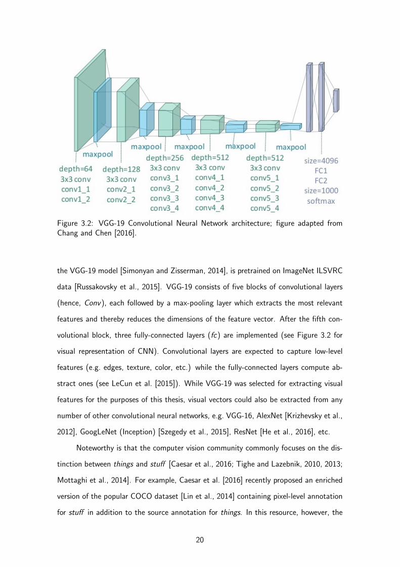
data [Russakovsky et al., 2015]. VGG-19 consists of five blocks of convolutional layers

(hence, Conv), each followed by a max-pooling layer which extracts the most relevant

features and thereby reduces the dimensions of the feature vector. After the fifth con-

volutional block, three fully-connected layers (fc) are implemented (see Figure 3.2 for

visual representation of CNN). Convolutional layers are expected to capture low-level

features (e.g. edges, texture, color, etc.) while the fully-connected layers compute ab-

stract ones (see LeCun et al. [2015]). While VGG-19 was selected for extracting visual

features for the purposes of this thesis, visual vectors could also be extracted from any

number of other convolutional neural networks, e.g. VGG-16, AlexNet [Krizhevsky et al.,

2012], GoogLeNet (Inception) [Szegedy et al., 2015], ResNet [He et al., 2016], etc.

Noteworthy is that the computer vision community commonly focuses on the dis-

tinction between things and stuff [Caesar et al., 2016; Tighe and Lazebnik, 2010, 2013;

Mottaghi et al., 2014]. For example, Caesar et al. [2016] recently proposed an enriched

version of the popular COCO dataset [Lin et al., 2014] containing pixel-level annotation

for stuff in addition to the source annotation for things. In this resource, however, the

20

stuff class does not align with the mass category defined linguistically. To illustrate, the

stuff class contains nouns such as mirror, door, table, tree, mountain, and house, which

are count nouns from a linguistic perspective. As a consequence, using existing resources

is not feasible for the purposes of this project, and we move on to the construction of

an appropriate dataset for this study.

21

4. Dataset

This chapter discusses the construction of the dataset used for the various experi-

ments presented herein. In addition to the previously mentioned WordNet [Miller, 1995]

which provides linguistic information, ImageNet [Deng et al., 2009] is utilized in order

to provide the link to the computer vision side. ImageNet is a resource that maps noun

senses from WordNet to their corresponding images. “ImageNet aims to populate the

majority of the 80,000 synsets of WordNet with an average of 500-1000 clean and full

resolution images. This will result in tens of millions of annotated images organized by

the semantic hierarchy of WordNet” [Deng et al., 2009]. Bounding box annotations are

available for a subset of the synsets available in ImageNet and are performed and verified

by hand using Amazon Mechanical Turk.

In order to obtain mass/count categorization of nouns, and more specifically cat-

egorization of their respective senses, the Bochum English Countability Lexicon (BECL)

[Kiss et al., 2016] is used. This resource maps synsets within WordNet to their respective

countability classes, with noun senses annotated as either mass, count, both, or neither

based on a series of syntactic patterns. Since the intention is to approach the matter

from a vision perspective, we first check how many of the labeled synsets are available

within ImageNet, with an additional requirement that the images have available bound-

ing box annotations. Bounding boxes are necessary in order to crop the images so that

only the region of interest, namely the object, remains. Among the available synsets are

36 mass, 58 both, and a remarkable 686 count. This could well be a byproduct of the

22

Figure 4.1: Various steps performed in building the dataset. Cropped image examplesare presented on the far right, with their respective (overlaid) bounding box annotationsvisible immediately to the left.

fact that count objects are seemingly easier to annotate with bounding boxes given that

they are discrete instances and are more often present in the foreground of an image.

For this reason, it could also be argued that more pictures are taken of count objects

in general, which could explain the synset availability bias within ImageNet regarding

mass/count nouns.

Investigation into the synsets annotated as mass reveals entities such as various

sports (soccer, basketball, etc.) whose corresponding images depict countable entities

such as players or balls. We also encounter collective nouns such as equipment, furni-

ture, luggage, housing, and artwork, which are merely collections of countable objects.

Other examples include nouns such as radio that, while the labeled sense can indeed

be described as mass, in this case a “medium of communication,” the images extracted

from ImageNet are instead of the more concrete count sense of a radio set. Similarly,

the abstract concept of housing provides images of houses. After later implementing a

second exclusion criterion for animacy, we are left with very few pure mass candidates

23

#syns #uniq nouns #imgs (avg) #imgs (range) OANC freq (avg) OANC freq (range)

mass 58 56 214.66 64 - 705 112.6 10 - 447count 58 53 303.93 60 - 1467 1556.17 624 - 4121

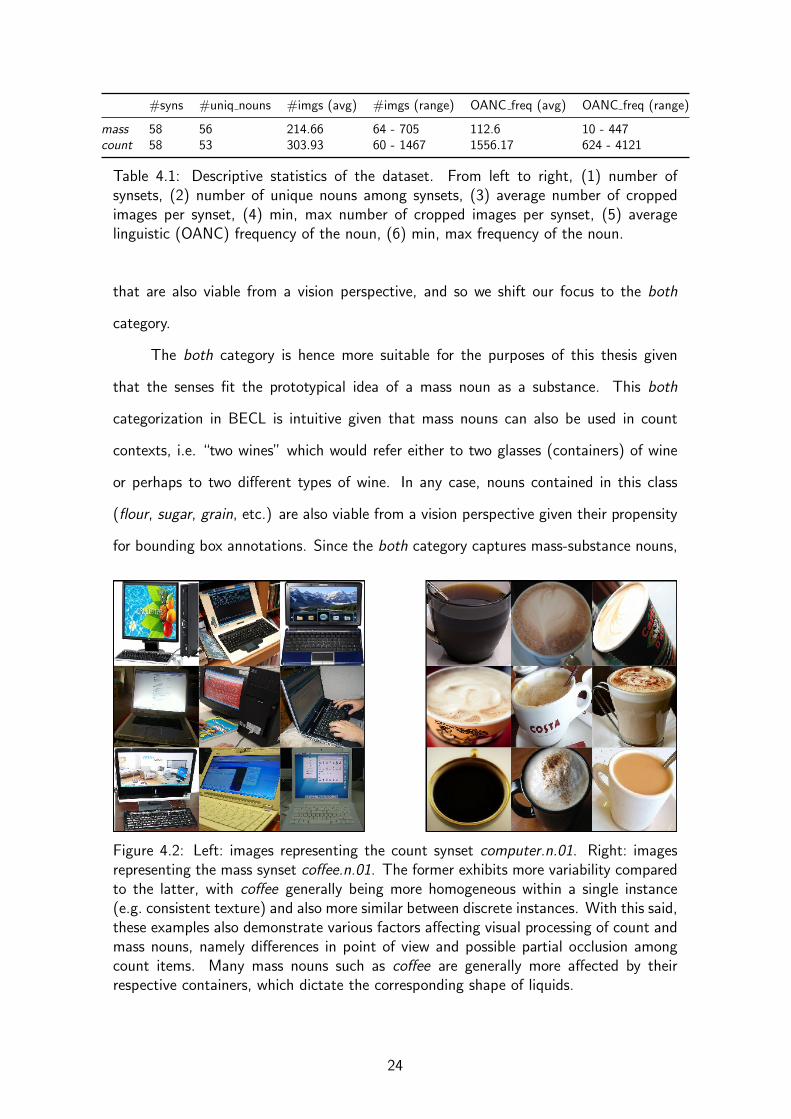
Table 4.1: Descriptive statistics of the dataset. From left to right, (1) number ofsynsets, (2) number of unique nouns among synsets, (3) average number of croppedimages per synset, (4) min, max number of cropped images per synset, (5) averagelinguistic (OANC) frequency of the noun, (6) min, max frequency of the noun.

that are also viable from a vision perspective, and so we shift our focus to the both

category.

The both category is hence more suitable for the purposes of this thesis given

that the senses fit the prototypical idea of a mass noun as a substance. This both

categorization in BECL is intuitive given that mass nouns can also be used in count

contexts, i.e. “two wines” which would refer either to two glasses (containers) of wine

or perhaps to two different types of wine. In any case, nouns contained in this class

(flour, sugar, grain, etc.) are also viable from a vision perspective given their propensity

for bounding box annotations. Since the both category captures mass-substance nouns,

Figure 4.2: Left: images representing the count synset computer.n.01. Right: imagesrepresenting the mass synset coffee.n.01. The former exhibits more variability comparedto the latter, with coffee generally being more homogeneous within a single instance(e.g. consistent texture) and also more similar between discrete instances. With this said,these examples also demonstrate various factors affecting visual processing of count andmass nouns, namely differences in point of view and possible partial occlusion amongcount items. Many mass nouns such as coffee are generally more affected by theirrespective containers, which dictate the corresponding shape of liquids.

24

Figure 4.3: Illustration of image cropping according to ImageNet bounding boxes as wellas preprocessing by the Convolutional Neural Network. Cropping is performed accordingto the original bounding box on the far left, after which the CNN takes the largestpossible square from the center of the cropped object.

it is henceforth referred to simply as mass. Of these 58 mass noun senses none are

animate, and so to avoid any possible confounding effects due to animacy, the countable

objects are also constrained to be inanimate, choosing the 58 most frequent where

frequency is a BECL metric based on the Open American National Corpus (OANC).

Images for the 58 + 58 synsets are downloaded and cropped according to bounding box

annotations. Figure 4.1 illustrates the various steps followed to build the dataset, with

descriptive statistics of the dataset reported in Table 4.1. For a complete list of employed

synsets along with an individual breakdown of the dataset statistics, see Synsets used in

Appendix.

Figure 4.2 shows example cropped images of one count synset along with one

mass. These additional examples are provided to demonstrate various factors affecting

processing of count and mass nouns in the visual modality, namely differences in ori-

entation (point of view) and possible occlusion among count items. Many mass nouns

such as the presented coffee are generally more affected by their respective containers,

which dictate the corresponding shape of liquids.

Figure 4.3 shows a detailed description of the image transformations that go into

25

building the dataset and also how the CNN preprocesses the input. Cropping is per-

formed according to the bounding box annotations provided by ImageNet, after which

the VGG-19 implementation takes the largest possible square from the center of the

cropped object. This square is then resized to a standard 224 x 224 pixels to feed the

Convolutional Neural Network as input.

26

5. Experiments and results

As part of the investigation into a possible difference in the visual representations

of mass and count noun referents, three experiments are presented herein. The first

experiment looks at whether there is indeed a significant difference in the visual variance

of mass and count feature vectors, as extracted from a convolutional neural network.

The second looks at the degree to which these visual features can be exploited to classify

objects as either mass or count. The third experiment tests the feature of mass nouns of

being arbitrarily divisible from a computational perspective. In other words, the ability

to learn the countability of half objects is explored.

5.1 Experiment I: Mean variance of images6

To investigate the progression from the low-level, more concrete image features to

the more abstract representations, a deep Convolutional Neural Network (CNN) is used.

This state-of-the-art CNN, namely the VGG-19 model [Simonyan and Zisserman, 2014]

elaborated upon in Chapter 3, is pretrained on ImageNet ILSVRC data [Russakovsky

et al., 2015]. Four of the five convolutional blocks (Conv2 -Conv5) are evaluated by

extracting the outputs of the first and last layers for each block7 as well as the output

of the three fully-connected layers (fc6, fc7, and fc8). Convolutional layers are expected

6 This experiment was published in the Proceedings of the 12th International Conference on Com-putational Semantics (IWCS); see Smith et al. [2017].

7 The first Conv1 block, which has approximately 3.2M dimensions, is not considered due to com-putational constraints.

27

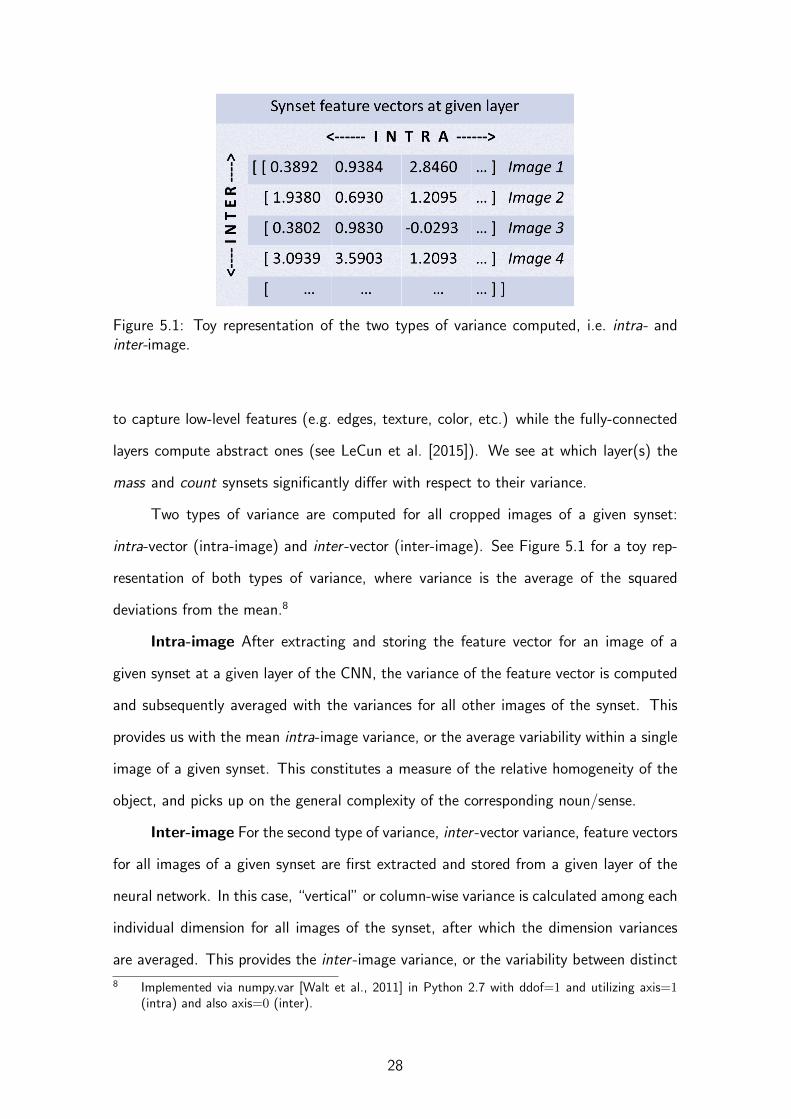
Figure 5.1: Toy representation of the two types of variance computed, i.e. intra- andinter-image.

to capture low-level features (e.g. edges, texture, color, etc.) while the fully-connected

layers compute abstract ones (see LeCun et al. [2015]). We see at which layer(s) the

mass and count synsets significantly differ with respect to their variance.

Two types of variance are computed for all cropped images of a given synset:

intra-vector (intra-image) and inter -vector (inter-image). See Figure 5.1 for a toy rep-

resentation of both types of variance, where variance is the average of the squared

deviations from the mean.8

Intra-image After extracting and storing the feature vector for an image of a

given synset at a given layer of the CNN, the variance of the feature vector is computed

and subsequently averaged with the variances for all other images of the synset. This

provides us with the mean intra-image variance, or the average variability within a single

image of a given synset. This constitutes a measure of the relative homogeneity of the

object, and picks up on the general complexity of the corresponding noun/sense.

Inter-image For the second type of variance, inter -vector variance, feature vectors

for all images of a given synset are first extracted and stored from a given layer of the

neural network. In this case, “vertical” or column-wise variance is calculated among each

individual dimension for all images of the synset, after which the dimension variances

are averaged. This provides the inter -image variance, or the variability between distinct

8 Implemented via numpy.var [Walt et al., 2011] in Python 2.7 with ddof=1 and utilizing axis=1(intra) and also axis=0 (inter).

28

Figure 5.2: Difference between mass/count variance through the various CNN layersin both inter- (blue, top) and intra- (orange, bottom) settings. The x axis shows thevarious layers while the y axis reports the ratio of average count versus mass synsetvariance. *** refers to a significant difference at p<.001, ** at p<.01, * at p<.05.

images of the same synset, which is a measure of the relative consistency between

instances of a given entity and its corresponding noun/sense.

Both types of variance are computed using the original, full-size vectors as ex-

tracted from the network.9 That is, no dimensionality reduction technique is utilized

which could result in information loss affecting the variance values. To determine whether

there is a significant difference between mass and count nouns, a two-tailed t-test is

performed for each type of variance and for each layer of the CNN.

Both intra-image and inter -image variances are found to be significantly lower

for mass nouns as compared to count nouns throughout all tested convolutional layers

up until Conv5 1, with only one exception (intra-image variance in Conv3 4). From

Conv5 4, in contrast, the difference becomes no longer significantly different, again with

just one exception (intra-image variance in fc7).

9 Vector size ranges from 1.6M dimensions of Conv2 to 1K dimensions of fc8.

29

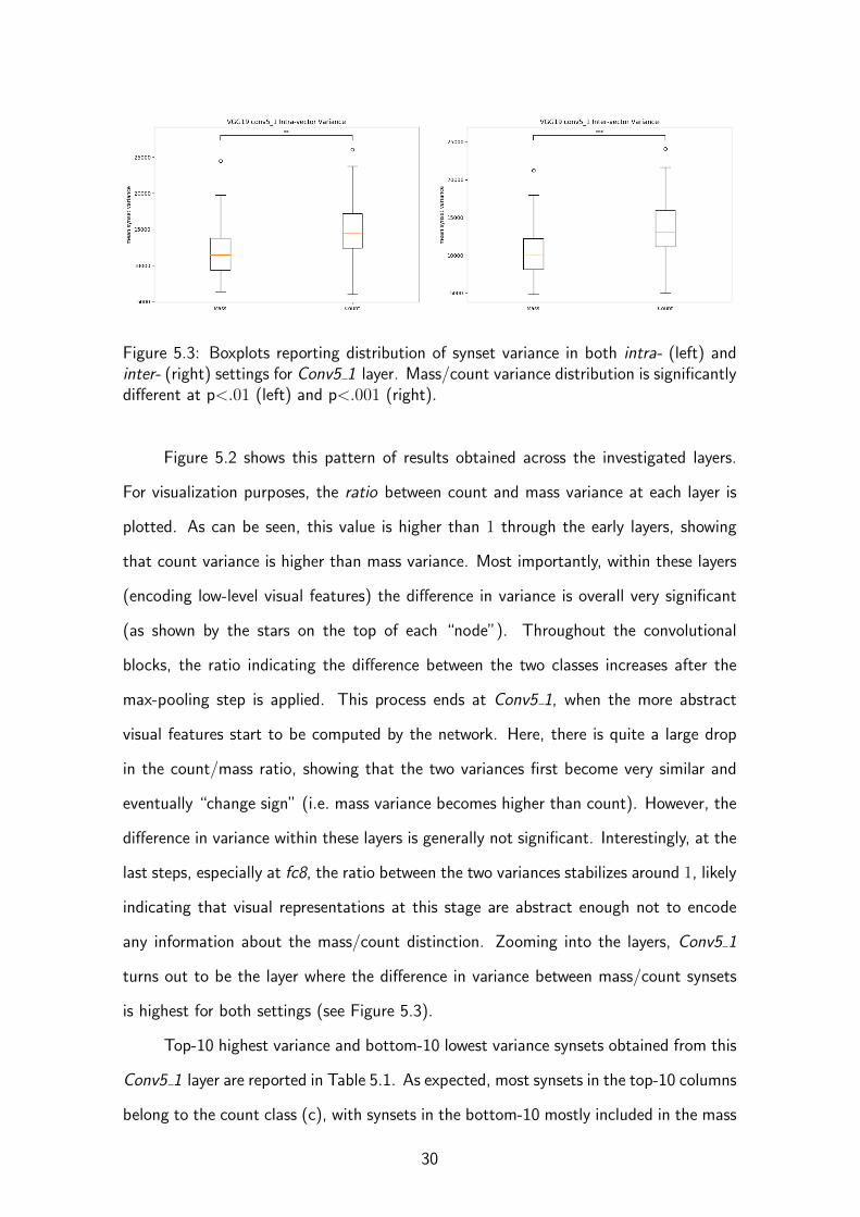
Figure 5.3: Boxplots reporting distribution of synset variance in both intra- (left) andinter- (right) settings for Conv5 1 layer. Mass/count variance distribution is significantlydifferent at p<.01 (left) and p<.001 (right).

Figure 5.2 shows this pattern of results obtained across the investigated layers.

For visualization purposes, the ratio between count and mass variance at each layer is

plotted. As can be seen, this value is higher than 1 through the early layers, showing

that count variance is higher than mass variance. Most importantly, within these layers

(encoding low-level visual features) the difference in variance is overall very significant

(as shown by the stars on the top of each “node”). Throughout the convolutional

blocks, the ratio indicating the difference between the two classes increases after the

max-pooling step is applied. This process ends at Conv5 1, when the more abstract

visual features start to be computed by the network. Here, there is quite a large drop

in the count/mass ratio, showing that the two variances first become very similar and

eventually “change sign” (i.e. mass variance becomes higher than count). However, the

difference in variance within these layers is generally not significant. Interestingly, at the

last steps, especially at fc8, the ratio between the two variances stabilizes around 1, likely

indicating that visual representations at this stage are abstract enough not to encode

any information about the mass/count distinction. Zooming into the layers, Conv5 1

turns out to be the layer where the difference in variance between mass/count synsets

is highest for both settings (see Figure 5.3).

Top-10 highest variance and bottom-10 lowest variance synsets obtained from this

Conv5 1 layer are reported in Table 5.1. As expected, most synsets in the top-10 columns

belong to the count class (c), with synsets in the bottom-10 mostly included in the mass

30

Conv5 1 intra- variance Conv5 1 inter- variancetop-10 bottom-10 top-10 bottom-10

magazine 01 (c) range 04 (c) magazine 01 (c) egg yolk 01 (m)salad 01 (m) dough 01 (m) shop 01 (c) range 04 (c)shop 01 (c) mountain 01 (c) salad 01 (m) dough 01 (m)church 02 (c) mesa 01 (c) machine 01 (c) mountain 01 (c)machine 01 (c) flour 01 (m) church 02 (c) mesa 01 (c)floor 02 (c) milk 01 (m) stage 03 (c) milk 01 (m)press 03 (c) glacier 01 (m) press 03 (c) flour 01 (m)stage 03 (c) butter 01 (m) floor 02 (c) butter 01 (m)pasta 01 (m) egg yolk 01 (m) brunch 01 (m) glacier 01 (m)brunch 01 (m) floor 04 (c) building 01 (c) sugar 01 (m)

Table 5.1: Synsets with highest (top-10) and lowest (bottom-10) variance in both intra-and inter- settings. Underlined synsets are those belonging to the lesser-represented classin each column. The bottom-10 columns are presented starting from lowest varianceand in ascending order.

class (m). Moreover, it can be noted that most of the synsets in the intra- setting also

appear in the inter- setting, at times with an almost perfect alignment. Finally, by

looking at the nouns that fall outside the expected pattern, it is possible to notice some

interesting cutting-edge cases (i.e. mass in top-10, count in bottom-10). Mountain and

range (here with the sense of “a series of hills or mountains”), for instance, are count

nouns whose visual texture is intuitively homogeneous, as well as salad and pasta which

are mass nouns referring to entities that inherently consist of many isolable parts, and

thus vary more on average across instances. For image examples of cropped objects from

the top- and bottom-3 synsets for each type of variance (keeping in mind that there is

a large overlap between the two types), see Example synset images in Appendix.

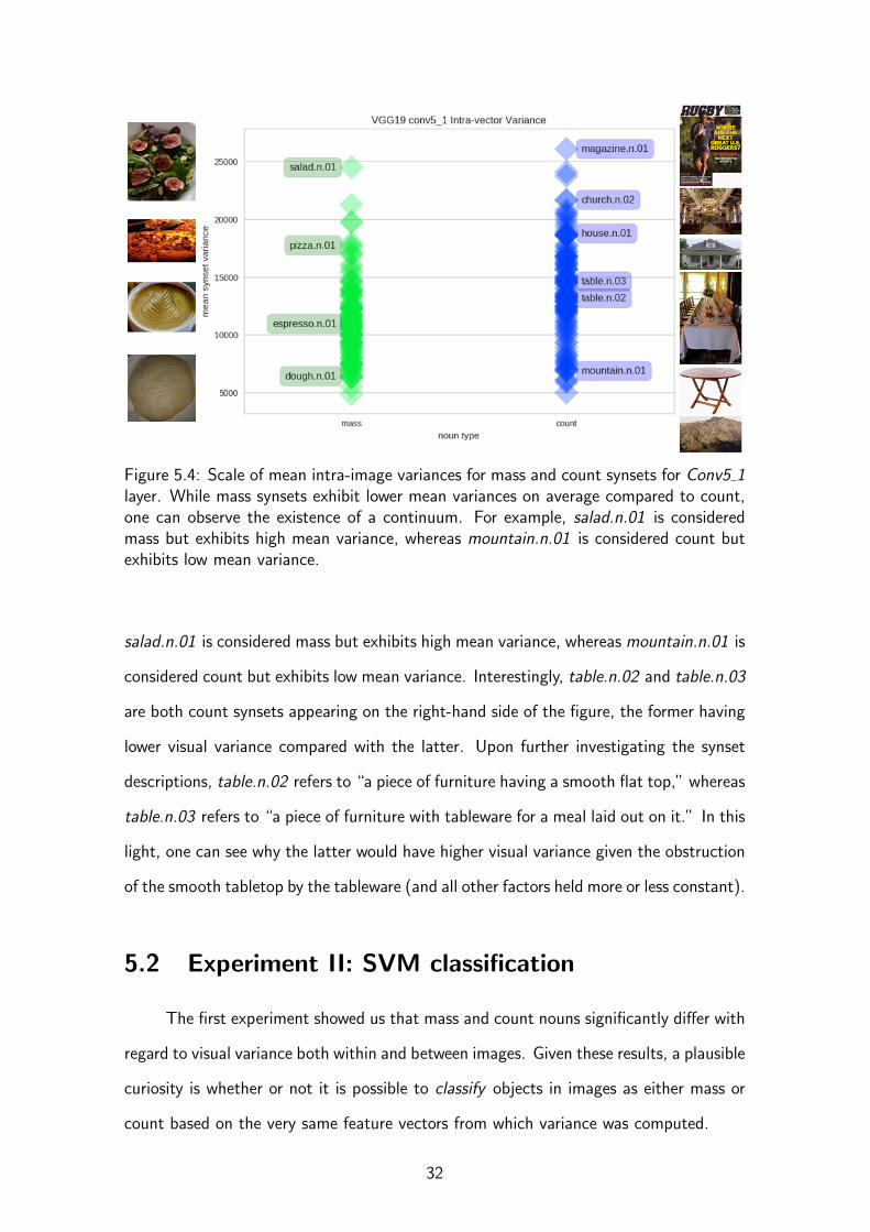
Figure 5.4 shows a scale of mean intra-image variances for mass and count synsets

for the Conv5 1 layer. This provides further evidence for the existence of a continuum of

countability which ranges from mass to count, from generally low visual variance to high

visual variance. Noteworthy also is that the same scale among mass and count synsets

is found with both types of variance, i.e. inter-image variance as well. Prototypical

examples such as the mass dough.n.01 which exhibits low visual variance as well as

the count magazine.n.01 with high visual variance coincide with the norm. With that

said, we also see the somewhat abnormal cases which fall somewhere along the way:

31

Figure 5.4: Scale of mean intra-image variances for mass and count synsets for Conv5 1layer. While mass synsets exhibit lower mean variances on average compared to count,one can observe the existence of a continuum. For example, salad.n.01 is consideredmass but exhibits high mean variance, whereas mountain.n.01 is considered count butexhibits low mean variance.

salad.n.01 is considered mass but exhibits high mean variance, whereas mountain.n.01 is

considered count but exhibits low mean variance. Interestingly, table.n.02 and table.n.03

are both count synsets appearing on the right-hand side of the figure, the former having

lower visual variance compared with the latter. Upon further investigating the synset

descriptions, table.n.02 refers to “a piece of furniture having a smooth flat top,” whereas

table.n.03 refers to “a piece of furniture with tableware for a meal laid out on it.” In this

light, one can see why the latter would have higher visual variance given the obstruction

of the smooth tabletop by the tableware (and all other factors held more or less constant).

5.2 Experiment II: SVM classification

The first experiment showed us that mass and count nouns significantly differ with

regard to visual variance both within and between images. Given these results, a plausible

curiosity is whether or not it is possible to classify objects in images as either mass or

count based on the very same feature vectors from which variance was computed.

32

CNN layerconv5 1 fc6 fc7 fc8

no norm 0.835 0.817 0.821 0.828norm 0 0.844 0.812 0.806 0.856norm 1 0.861 0.873 0.872 0.879

Table 5.2: Overall SVM accuracies trained to distinguish mass versus count from visualvectors. Various normalization techniques are explored among various CNN layers, andeach entry is an average of 10 random train/test data splits.

To this end, Support Vector Machine (SVM) classifiers are trained and tested10

to evaluate the hypothesis that indeed the mass versus count distinction should be

inherent in the visual vectors and yield overall high classification accuracies (while varying

slightly depending on layer). SVMs manipulate features into support vectors which map

datapoints into a high-dimensional space with a hyperplane separating the two classes to

the greatest extent possible (see for example Kotsiantis et al. [2007]). The previous 58

mass and 58 count synsets were randomly split 80%/20%, hence giving 47+47 training

synsets and 11 + 11 testing synsets. This random split was consistently repeated 10

times for each normalization and layer combination, after which resulting accuracies

were averaged for each. This provided an average training datapoint size of 24,600 and

average testing datapoints of 5,682 (or roughly an 81%/19% split in the end). Layers

selected for testing include each of the three fully-connected layers from VGG-19 (fc6,

fc7, fc8), partly due to their reduced dimensionality,11 as well as Conv5 1 which showed

the most significant difference in visual variance from the previous experiment.

To note, the data was split among synsets in order to make the classification a

bit more challenging, i.e. the split could have also been a simple 80%/20% split among

all datapoints, ignoring their respective synset labels. However, this would mean the

classifier would see examples of all synset classes in training, which could make the

classification task in testing significantly easier. Instead, the decision was made to test

the mass/count classification on novel synsets, or ones that have not been previously

seen by the system.

10 Linear kernel employed via sklearn.svm.LinearSVC (see Pedregosa et al. [2011]) in Python 2.7.11 4096, 4096, and 1000 dimensions respectively.

33

Two different normalization techniques12 of the feature vectors were tested: norm 0,

which normalizes by dimension, and the default norm 1 that normalizes by sample. This

is similar to the inter- and intra-vector variance, respectively, in that norm 0 normalizes

a single dimension at a time (among all samples), whereas norm 1 normalizes a single

sample at a time (independently of all other samples). This is compared against SVM

classification without any prior normalization of feature vectors (no norm).

It is clear from the data that the standard practice of normalizing vectors by

sample (norm 1) provides superior results. The accuracies presented in Table 5.2 show

the proportion of correctly-classified mass and count feature vectors. The best results

are obtained from the final fully-connected layer, fc8, which makes sense given that this

is the final layer before the CNN outputs the type of object in a given image. Since the

visual information has been made abstract at this level, the network is able to generalize

well about the countability of the respective objects as well. Also to note, Conv5 1 has

the highest classification accuracy for no norm which is expected from the results of

Experiment I: since the visual vectors vary the most between mass and count nouns at

this layer, it follows that these discrepancies can be exploited for classification in this

task. Furthermore, the normalization techniques can be said to confound the ability of

the classifier to capitalize on variance in the visual features, which gives the upper hand

to the fully-connected layers in the normalized settings.

5.3 Experiment III: Half ' whole?

We have previously seen that count nouns are atomic in nature, whereas mass

nouns generally are not. Following the same notion, mass nouns are said to be arbitrarily

divisible, meaning that if you divide flour, for example, you obtain (multiple instances of)

flour. This property for count nouns does not hold, as splitting a bicycle does not leave

you with multiple bicycles. In this experiment we aim to test whether convolutional neural

networks can make such a distinction. To this end, we test if the network can decide

whether an object is fully represented or not by the visual features of whole versus half

12 l2 ’soft’ normalization via sklearn.preprocessing.normalize utilizing default axis 1 and also axis 0.

34

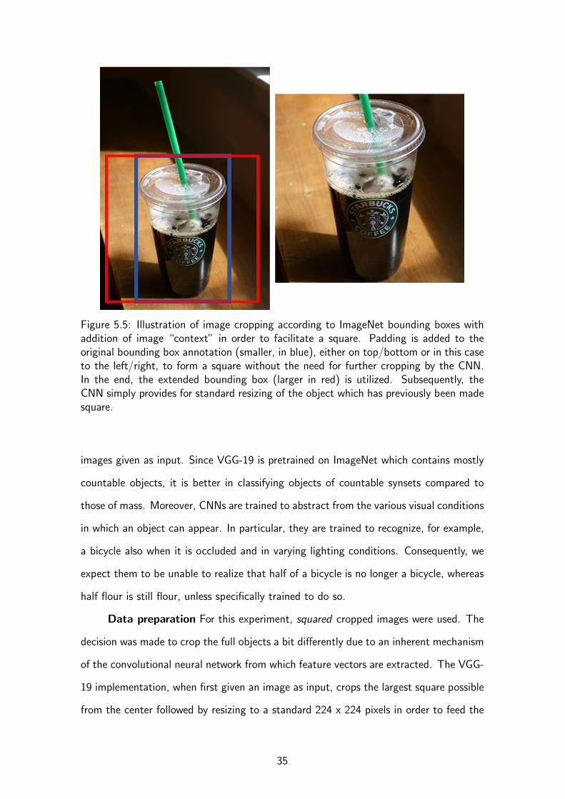
Figure 5.5: Illustration of image cropping according to ImageNet bounding boxes withaddition of image “context” in order to facilitate a square. Padding is added to theoriginal bounding box annotation (smaller, in blue), either on top/bottom or in this caseto the left/right, to form a square without the need for further cropping by the CNN.In the end, the extended bounding box (larger in red) is utilized. Subsequently, theCNN simply provides for standard resizing of the object which has previously been madesquare.

images given as input. Since VGG-19 is pretrained on ImageNet which contains mostly

countable objects, it is better in classifying objects of countable synsets compared to

those of mass. Moreover, CNNs are trained to abstract from the various visual conditions

in which an object can appear. In particular, they are trained to recognize, for example,

a bicycle also when it is occluded and in varying lighting conditions. Consequently, we

expect them to be unable to realize that half of a bicycle is no longer a bicycle, whereas

half flour is still flour, unless specifically trained to do so.

Data preparation For this experiment, squared cropped images were used. The

decision was made to crop the full objects a bit differently due to an inherent mechanism

of the convolutional neural network from which feature vectors are extracted. The VGG-

19 implementation, when first given an image as input, crops the largest square possible

from the center followed by resizing to a standard 224 x 224 pixels in order to feed the

35

Figure 5.6: Illustration of cropping of half images from the original object (which waspreviously cropped according to ImageNet bounding box annotations). Half cropping isperformed along the longest dimension of the original object, i.e. either along the y axis(left) or x axis (right).

first convolutional layer and proceed through the network. Given that we would like

to have the entire (full) object from the bounding box provided from ImageNet, the

bounding box is extended either on the x or y axis (if possible) in order to create a

square before feeding the CNN (see Figure 5.5). If the original image does not provide

for extending the bounding box as a square, this bounding box is discarded.13

In adding this so-called context to the image, we avoid any possible partial cropping

of the full object in order to make it square, and hence the network simply provides for

the resizing of the (already square) image. While adding this context could indeed have

a mild impact on the feature vectors to be extracted, either by adding distractive “noise”

or by adding clues to the identity of a given object (think salt placed beside pepper, for

example), this is balanced by the fact that for this experiment full representations of

whole objects are essential, and the preservation of the external shape necessitates this

method.

To note, the cropping of half objects is done simply from the original bounding

boxes (see Figure 5.6). Cropping half objects from the squared full objects would not

make sense given that half of a square is no longer a square. Therefore, it is better to

13 Average number of mass cropped images drops from 214.66 to 150.28 when squaring, while meannumber of count cropped images drops from 303.93 to 110.76.

36

slice the original bounding boxes in half along the longest dimension. Also, even if a

small portion of these half images is discarded by the CNN in order to make a square, it

is still seeing a significant part of the original object which is perfectly acceptable for our

purposes. Noteworthy is that only half objects which have available (squared) full objects

are utilized going forward. In addition, the above cropping guidelines were only applied

to images with a single bounding box annotation, i.e. images with a single instance

of the given object, in order to avoid confounding effects of overlapping annotations or

possible multiple annotations of a single object instance. Feature vectors were computed

via VGG-19 both for the squared full objects as well as for their half counterparts. In each

of the forthcoming network configurations, normalized feature vectors are utilized.14

To note, the following experiment was originally performed using visual features

both from Conv5 1 as well as from fc7. In this case, the Conv5 1 results showed the

same trends as did those from fc7 but simply to a lesser extent. This is intuitive given

that the later fully-connected layers of the network encode more abstract information

about the object class, which of course also helps in our synset classification. For this

reason, the focus of this experiment will be to report the fc7 findings which are similar

to but more pronounced than the findings from the earlier convolutional layer. Training,

validation, and testing data are split 70/10/20% among each individual synset in order

to guarantee that images from each synset are a part of each phase. Validation data is

utilized to help achieve maximum generalization from the network, providing the ability

to discontinue training when the network starts to overfit on the training data.15

Classification The normalized feature vectors are subsequently fed to a three-

layer neural network. The first two hidden layers serve to map the visual vector to its

corresponding synset (and hence indirectly to its corresponding countability class). To

some extent, this is a method for reengineering the final fully-connected layers of VGG-19

in order to obtain classification specifically for our 58 mass and 58 count synsets. The

third and final additional layer is a softmax layer which serves to output probabilities

that a given image belongs to each possible synset, which is compared with a one-hot

14 Normalization by sample (norm 1 from Experiment II).15 The number of epochs is optimized for each configuration, ranging from 11 to 25 and utilizing

dropout to help avoid overfitting.

37

whole image half imagetop1 top2 top3 top1 top2 top3

fc7overall 0.631 0.783 0.843 0.462 0.612 0.686count 0.689 0.839 0.899 0.507 0.672 0.745mass 0.557 0.713 0.772 0.405 0.537 0.611

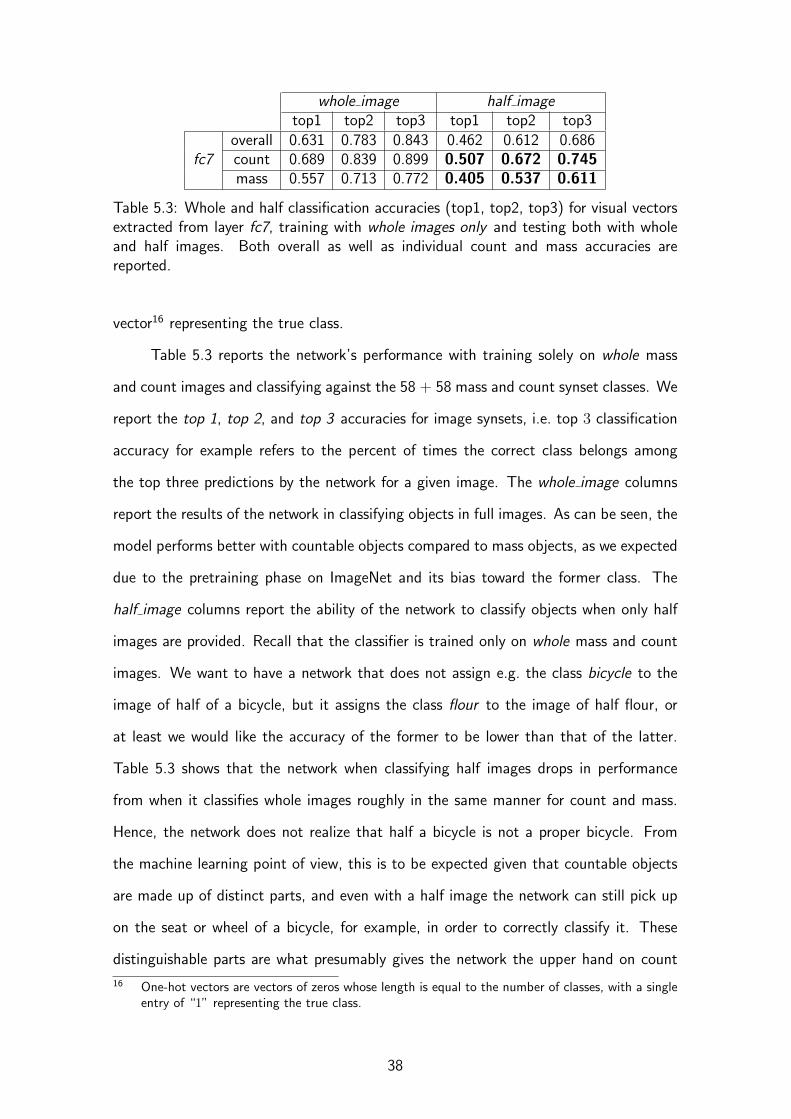
Table 5.3: Whole and half classification accuracies (top1, top2, top3) for visual vectorsextracted from layer fc7, training with whole images only and testing both with wholeand half images. Both overall as well as individual count and mass accuracies arereported.

vector16 representing the true class.

Table 5.3 reports the network’s performance with training solely on whole mass

and count images and classifying against the 58 + 58 mass and count synset classes. We

report the top 1, top 2, and top 3 accuracies for image synsets, i.e. top 3 classification

accuracy for example refers to the percent of times the correct class belongs among

the top three predictions by the network for a given image. The whole image columns

report the results of the network in classifying objects in full images. As can be seen, the

model performs better with countable objects compared to mass objects, as we expected

due to the pretraining phase on ImageNet and its bias toward the former class. The

half image columns report the ability of the network to classify objects when only half

images are provided. Recall that the classifier is trained only on whole mass and count

images. We want to have a network that does not assign e.g. the class bicycle to the

image of half of a bicycle, but it assigns the class flour to the image of half flour, or

at least we would like the accuracy of the former to be lower than that of the latter.

Table 5.3 shows that the network when classifying half images drops in performance

from when it classifies whole images roughly in the same manner for count and mass.

Hence, the network does not realize that half a bicycle is not a proper bicycle. From

the machine learning point of view, this is to be expected given that countable objects

are made up of distinct parts, and even with a half image the network can still pick up

on the seat or wheel of a bicycle, for example, in order to correctly classify it. These

distinguishable parts are what presumably gives the network the upper hand on count

16 One-hot vectors are vectors of zeros whose length is equal to the number of classes, with a singleentry of “1” representing the true class.

38

predicted classcount mass precision recall f-score

actualclass

count 2744 142 0.912 0.951 0.931mass 265 2015 0.934 0.884 0.908

predicted classcount whole mass whole precision recall f-score

actualclass

count whole 938 24 0.953 0.975 0.964mass whole 46 714 0.967 0.939 0.953

predicted classcount half mass half precision recall f-score

actualclass

count half 1806 118 0.892 0.939 0.915mass half 219 1301 0.917 0.856 0.885

Table 5.4: Confusion matrices for count versus mass classification via fc7 visual vectors,training with whole images only and testing both with whole and half images. Thecountability prediction here is indirect given that the model classifies a given image to asynset and hence indirectly as count or mass. The countability classification is consideredcorrect even if the synset classification is incorrect as long as the predicted synset stillbelongs to the target countability class. Overall results are reported (top) as well as theseparate confusion matrices for whole (middle) and half images (bottom).

objects in general.

Table 5.4 shows the confusion matrix for this network, providing a somewhat

simplified look into mass versus count discrimination ability of this network configuration.

Note that the countability prediction here is indirect given that the model classifies

a given image to a synset and hence indirectly as count or mass. The countability

classification is considered correct even if the synset classification is incorrect as long as

the predicted synset still belongs to the target countability class. Granularity is also added

by further separating the overall mass versus count distinction into distinct confusion

matrices for whole and half images.17

Finally, we investigate whether we can explicitly train the network away from

this countable tendency in favor of a more theoretical understanding. Table 5.5 shows

classification accuracies for other training settings of the same network architecture,

namely that in these settings half images are added to the training phase, still using fc7

feature vectors. An important difference in these two configurations is that 58 additional

17 Note that the same images are used in whole and half testing, and hence the doubling of thenumber of test half images compared to whole.

39

whole image half imagetop1 top2 top3 top1 top2 top3

fc7half count train

overall 0.577 0.746 0.810 0.439 0.586 0.663count 0.597 0.777 0.840 0.534 0.701 0.786mass 0.550 0.702 0.764 0.318 0.440 0.506

fc7half count +

half mass train

overall 0.598 0.763 0.817 0.499 0.657 0.739count 0.610 0.780 0.832 0.502 0.669 0.758mass 0.580 0.739 0.795 0.497 0.642 0.715

Table 5.5: Whole and half classification accuracies (top1, top2, top3) for visual vectorsextracted from layer fc7 with different training settings. half count train includes halfcount images in training, while half count + half mass train includes half count as wellas half mass objects in training. Both overall as well as individual count and massaccuracies are reported.

synset classes are added for half count images. Classes for half mass images are not

necessary or appropriate since half mass images should predict the regular (full) mass

synset/class. Given that the neural network is good at classifying half count images

from the previous configuration, the extra classes are added and half count images

added to training in an attempt to explicitly train the network that half count objects

are different from–and should not belong to–their whole synset counterparts. In the first

half count train configuration, only half count images are added to training, while in the

second half count + half mass train setting both half count as well as half mass images

are added to training.18 As can be noted in the bolded figures of the table, while we

checked in the first setting if the network is able to generalize on its own about half mass

images, it is evident that training examples of both types of half images are necessary in

order for the network to be able to generalize (i.e. 31.8% versus 49.7% top1 accuracy

for half mass images between the two settings).

Table 5.6 shows the confusion matrices for these two network configurations,

half count train and half count + half mass train. Note the mass whole and mass half

prediction classes are collapsed simply into mass given our premise that there is no

significant cognitive distinction between flour and half flour, for example. In the end

the half classification accuracies in the final setting are more or less the same for count

and mass (50.2% versus 49.7% top1 accuracies respectively), showing that with explicit

18 In this case, whole image data points are used twice in training in order to balance the number oftheir half image counterparts.

40

predicted classcount whole mass count half precision recall f-score

actualclass

count whole 767 20 175 0.730 0.797 0.762mass whole 34 696 30

0.973 0.714 0.823mass half 22 931 567count half 227 26 1671 0.684 0.869 0.765

predicted classcount whole mass count half precision recall f-score

actualclass

count whole 795 33 134 0.721 0.826 0.770mass whole 29 717 14

0.933 0.922 0.927mass half 19 1385 116count half 260 118 1546 0.854 0.804 0.828

Table 5.6: Confusion matrices for count versus mass classification with training onhalf images in addition to whole images, still utilizing fc7 feature vectors. Results arereported for a network trained on half count images only (half count train, top) andalso for a network trained both on half count as well as half mass images (half count +half mass train, bottom). Testing occurs also both with whole and half images, but notethe mass whole and mass half prediction classes are collapsed simply into mass givenour premise that there is no significant cognitive distinction between flour and half flour,for example.

training on half objects the network is able to generalize equally well between these

countability classes. Therefore, the cognition-based hypothesis for this experiment is

not directly confirmed by the results which show that half count synset classification is

generally more accurate than that of half mass. Again, this is simply a product of the

fact that the convolutional neural network is previously trained on ImageNet and picks

up on distinct parts and pieces of items in order to correctly classify them. However,

the results indeed show that with explicit half training the network is able to generalize

equally well between half mass and half count objects. In this light, the network can

learn that half of a bicycle is no longer a proper bicycle whereas half of a given instance

of flour is still flour when explicitly taught. Therefore, we still hold that half mass objects

are more similar to their whole counterparts than for count.

41

6. Discussion and future work

In Experiment I, mass-substance nouns are shown to have significantly lower intra-

and inter-image variance than do count nouns, which manifests itself throughout the

early convolutional layers of a state-of-the-art CNN. This could be useful in applica-

tions such as Visual Question Answering (VQA) or image caption generation, where a

proper understanding of countability can lead to better responses and descriptions. Also,

the results of this work could be combined with current research on quantification in

Language and Vision, with a sort of multi-task approach: correct understanding of the

countability of an object could aid in the task of quantifying it, and vice versa.

With that said, one can also see that there are cases which lie somewhere in

the middle, exhibiting visual properties belonging to the opposing mass/count class.

Interestingly, count nouns which are labeled as “stuff” in the things vs. stuff distinction,

namely mountain, door, etc., are found to behave more like mass. More in general,

there seems to be a visual continuum ranging from mass-substance all the way to count

nouns. Similarly, recent studies in linguistics point to the fact that the distribution of

nouns with respect to their syntactic contexts of occurrence is not consistent with a

dichotomist division of the lexicon in two clear-cut classes of mass and count nouns

[Zanini et al., 2016]. Also, metalinguistic judgments collected in various languages point

to an interpretation of mass and count nouns as poles of a continuous distribution

[Kulkarni et al., 2013]. Further investigations on the relation between the visual features

of referents and cross-linguistic features are thus desirable.

42

In this light, a possible extension of this work on mass and count representations

in the visual modality lies in cross-linguistic countability of nouns. In other words, the

correlation between visual features such as variance and a given noun’s countability usage

in (multilingual) corpora could be explored. Given that it has been shown that mass and

count usage of nouns indeed has a significant basis in vision, the hypothesis would be

that the prototypical nouns from a vision perspective, i.e. mass nouns with low visual

variance and count nouns with high visual variance, would have consistent countability

uses across languages, i.e. always mass or always count. Likewise, irregular nouns from

a vision perspective, i.e. mass nouns with high visual variance and count nouns with low

visual variance, would be those that vary linguistically from one language to another.

Experiment II further capitalizes on these various distinctions between mass and

count objects in the visual modality to show that countability classification based on

visual features is indeed possible and in general yields high accuracies overall. A desired

extension of this experiment would be to make the SVM results more fine-grained as

well, reporting separate classification accuracies for mass as well as count objects, in

addition to the current overall figures.

Regarding Experiment III, the Convolutional Neural Network is in the end very

robust to changes such as in point of view and possible partial occlusion of objects

given that it is previously exposed to many thousands of images from ImageNet. In

this light, the CNN is already set in its way, and the extracted feature vectors are very

much characteristic of this exhaustive training. For this reason, the network is able to

pick up on parts of half-count items, for example, and still correctly classify them to

their corresponding synsets. With that said, with explicit training of the network both

on half-mass and half-count items, we achieve an acceptable result. A future extension

of this work could be to train a CNN from scratch with a dataset of mass and count

images to further advance the goals of this experiment and of this study in general.

43

Acknowledgments

A tremendous thanks to my supervisors Raffaella Bernardi and Inaki Inza and

also to Sandro Pezzelle for their invaluable insight as well as oversight. In addition, I

am grateful to the Erasmus Mundus European Master in Language and Communication

Technologies (EM LCT) for the scholarship provided for my participation in this program.

44

7. Appendix

7.1 Example synset images

Figure 7.1: Example images of magazine.n.01.

45

Figure 7.2: Example images of salad.n.01.

Figure 7.3: Example images of shop.n.01.

46

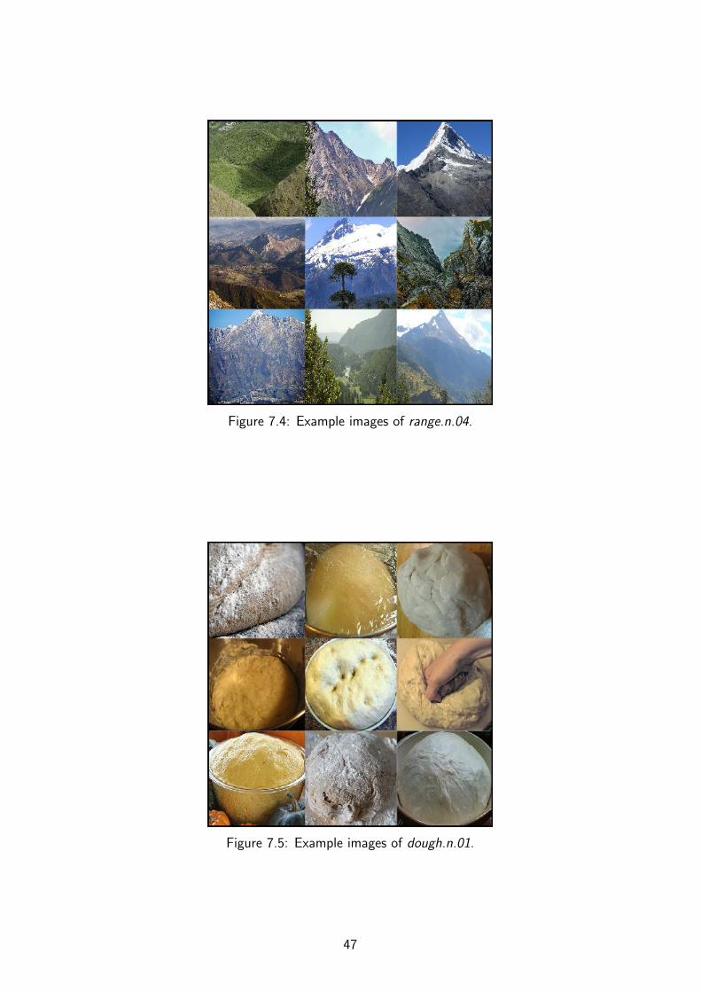
Figure 7.4: Example images of range.n.04.

Figure 7.5: Example images of dough.n.01.

47

Figure 7.6: Example images of mountain.n.01.

Figure 7.7: Example images of egg yolk.n.01.

48

7.2 Synsets used

Table 7.1: List of 58 mass + 58 count synsets used, with each class sorted by Open Amer-ican National Corpus (OANC) frequency in descending order. To note, some synsetshave multiple surface forms (lemmata) appearing in corpora, e.g. certain uses of soil anddirt both correspond to the soil.n.02 synset and hence to its corresponding images. Forthese synsets, only the most frequent lemma based on OANC frequency is presented.Noteworthy is that the listed synsets are clickable in the digital version, linking to thecorresponding ImageNet pages which provide synset descriptions and example imagesamong other information.

type lemma synset #images OANC freq

mass port port.n.02 142 447

mass soil soil.n.02 235 398

mass milk milk.n.01 196 386

mass sand sand.n.01 205 362

mass coffee coffee.n.01 159 356

mass coffee coffee.n.02 70 356

mass bread bread.n.01 145 277

mass cream cream.n.03 178 271

mass sugar sugar.n.01 130 267

mass rice rice.n.01 167 262

mass fabric fabric.n.01 151 259

mass wire wire.n.01 191 195

mass cotton cotton.n.02 199 166

mass grain grain.n.02 97 163

mass sauce sauce.n.01 151 147

mass salad salad.n.01 181 143

mass soy soy.n.04 70 139

mass juice juice.n.01 205 129

mass pizza pizza.n.01 604 118

mass butter butter.n.01 176 116

49

Table 7.1: List of 58 mass + 58 count synsets used, continued.

type lemma synset #images OANC freq

mass honey honey.n.01 398 109

mass rope rope.n.01 388 109

mass canvas canvas.n.01 64 106

mass soup soup.n.01 386 102

mass pottery pottery.n.01 251 98

mass candy candy.n.01 87 87

mass wheat wheat.n.01 73 86

mass yolk egg yolk.n.01 240 83

mass flour flour.n.01 201 49

mass pasta pasta.n.01 188 48

mass champagne champagne.n.01 383 47

mass dough dough.n.01 497 45

mass rose blush wine.n.01 152 45

mass tonic pop.n.02 184 37

mass pudding pudding.n.03 264 33

mass pudding pudding.n.01 160 33

mass gin gin.n.01 117 33

mass lettuce lettuce.n.03 297 32

mass chili chili.n.01 182 28

mass salsa salsa.n.01 182 26

mass gravel gravel.n.01 356 25

mass ade fruit drink.n.01 189 25

mass syrup syrup.n.01 129 25

mass yogurt yogurt.n.01 164 24

mass whiskey whiskey.n.01 124 23

mass glacier glacier.n.01 132 22

50

Table 7.1: List of 58 mass + 58 count synsets used, continued.

type lemma synset #images OANC freq

mass barley barley.n.01 80 22

mass pastry pastry.n.01 202 21

mass liqueur liqueur.n.01 169 21

mass brunch brunch.n.01 173 20

mass brandy brandy.n.01 160 19

mass casserole casserole.n.01 149 18

mass cocoa cocoa.n.01 178 16

mass ale ale.n.01 213 14

mass lotion lotion.n.01 705 11

mass espresso espresso.n.01 656 11

mass lemonade lemonade.n.01 134 11

mass vino wine.n.01 191 10

count paper newspaper.n.01 445 4121

count house house.n.01 178 4067

count mouse mouse.n.04 532 3965

count structure structure.n.01 142 3114

count room room.n.01 186 2605

count computer computer.n.01 229 2596

count guy guy.n.03 117 2460

count range range.n.04 177 2241

count center center.n.03 175 2215

count step step.n.04 277 2210

count plant plant.n.02 332 2170

count plant plant.n.01 204 2170

count building building.n.01 341 2140

count tv television receiver.n.01 185 1867

51

Table 7.1: List of 58 mass + 58 count synsets used, continued.

type lemma synset #images OANC freq

count magazine magazine.n.01 478 1838

count stage stage.n.03 480 1825

count papers document.n.01 268 1791

count weight weight.n.02 183 1723

count street street.n.01 528 1700

count street street.n.02 504 1700

count gun gun.n.01 223 1669

count call call.n.01 176 1661

count press press.n.03 166 1548

count phone earphone.n.01 586 1522

count phone telephone.n.01 308 1522

count file file.n.03 462 1470

count store shop.n.01 183 1401

count road road.n.01 171 1401

count store memory.n.04 157 1401

count church church.n.02 468 1368

count box box.n.01 382 1263

count table table.n.02 489 1249

count table table.n.03 334 1249

count table mesa.n.01 131 1249

count arm weapon.n.01 153 1233

count restaurant restaurant.n.01 1467 1196

count sign sign.n.02 573 1169

count sign signboard.n.01 202 1169

count door door.n.01 465 1159

count door door.n.04 197 1159

52

Table 7.1: List of 58 mass + 58 count synsets used, continued.

type lemma synset #images OANC freq

count machine machine.n.04 141 1022

count floor floor.n.04 389 993

count floor floor.n.02 60 993

count radio radio receiver.n.01 135 964

count window window.n.01 346 932

count complex building complex.n.01 174 916

count fire fire.n.04 201 848

count mountain mountain.n.01 241 826

count plane airplane.n.01 459 824

count diet diet.n.03 178 792

count video video recording.n.01 169 792

count boat boat.n.01 272 758

count apartment apartment.n.01 133 715

count flower flower.n.01 236 696

count bed bed.n.01 346 682

count filter filter.n.01 419 666

count bag bag.n.01 311 639

count temple temple.n.01 164 624

53

Bibliography

Abraham, A. (2005). Artificial neural networks. Handbook of measuring system design.

Barner, D. and Snedeker, J. (2005). Quantity judgments and individuation: Evidence

that mass nouns count. Cognition, 97(1):41–66.

Brown, R. and Berko, J. (1960). Word association and the acquisition of grammar.

Child Development, pages 1–14.

Caesar, H., Uijlings, J., and Ferrari, V. (2016). COCO-Stuff: Thing and Stuff Classes

in Context. arXiv preprint arXiv:1612.03716.

Cameron, W. B. (1963). Informal sociology: A casual introduction to sociological

thinking, volume 21. Random House.

Chang, M. and Chen, Y.-N. (2016). Applied Deep Learning - Convolutional Neu-

ral Networks. https://www.csie.ntu.edu.tw/~yvchen/f105-adl/doc/161103_

ConvolutionalNN.pdf. [Online; accessed 17-Sept-2017].

Cheng, C.-Y. (1973). Comments on Moravcsik’s paper. In Approaches to natural lan-

guage, pages 286–288. Springer.

Chierchia, G. (1998). Reference to kinds across language. Natural language semantics,

6(4):339–405.

Chierchia, G. (2010). Mass nouns, vagueness and semantic variation. Synthese,

174(1):99–149.

Clark, E. V. (1995). The lexicon in acquisition, volume 65. Cambridge University Press.

54

Deng, J., Dong, W., Socher, R., Li, L.-J., Li, K., and Fei-Fei, L. (2009). ImageNet: A

large-scale hierarchical image database. In Computer Vision and Pattern Recognition,

2009. CVPR 2009. IEEE Conference on, pages 248–255. IEEE.

Doron, E. and Muller, A. (2010). The cognitive basis of the mass-count distinction: Ev-

idence from bare nouns. Abstract. The Hebrew University of Jerusalem and University

of Sao Paolo.

Fieder, N., Nickels, L., and Biedermann, B. (2014). Representation and processing of

mass and count nouns: a review. Frontiers in psychology, 5.

He, K., Zhang, X., Ren, S., and Sun, J. (2016). Deep residual learning for image

recognition. In Proceedings of the IEEE conference on computer vision and pattern

recognition, pages 770–778.

Iwasaki, N., Vinson, D. P., and Vigliocco, G. (2010). Does the grammatical count/mass

distinction affect semantic representations? Evidence from experiments in English and

Japanese. Language and Cognitive Processes, 25(2):189–223.

Khaligh-Razavi, S.-M. and Kriegeskorte, N. (2014). Deep supervised, but not unsuper-

vised, models may explain IT cortical representation. PLoS computational biology,

10(11):e1003915.

Kiss, T., Pelletier, F. J., Husic, H., Poppek, J. M., and Simunic, R. N. (2016). A Sense-

Based Lexicon for Count and Mass Expressions: The Bochum English Countability

Lexicon. In Proceedings of LREC 2016.

Kotsiantis, S. B., Zaharakis, I., and Pintelas, P. (2007). Supervised machine learning:

A review of classification techniques.

Krizhevsky, A., Sutskever, I., and Hinton, G. E. (2012). Imagenet classification with deep

convolutional neural networks. In Advances in neural information processing systems,

pages 1097–1105.

55

Kulkarni, R., Rothstein, S., and Treves, A. (2013). A statistical investigation into the

cross-linguistic distribution of mass and count nouns: Morphosyntactic and semantic

perspectives. Biolinguistics, 7:132–168.

LeCun, Y., Bengio, Y., and Hinton, G. (2015). Deep learning. Nature, 521(7553):436–

444.

Lin, T.-Y., Maire, M., Belongie, S., Hays, J., Perona, P., Ramanan, D., Dollar, P., and

Zitnick, C. L. (2014). Microsoft COCO: Common objects in context. In European

Conference on Computer Vision, pages 740–755. Springer.

MacNamara, J. (1972). Cognitive basis of language learning in infants. Psychological

review, 79(1):1.

Malt, B. C., Sloman, S. A., Gennari, S., Shi, M., and Wang, Y. (1999). Knowing versus

naming: Similarity and the linguistic categorization of artifacts. Journal of Memory

and Language, 40(2):230–262.

Middleton, E. L., Wisniewski, E. J., Trindel, K. A., and Imai, M. (2004). Separating the

chaff from the oats: Evidence for a conceptual distinction between count noun and

mass noun aggregates. Journal of Memory and Language, 50(4):371–394.

Miller, G. A. (1995). WordNet: a lexical database for English. Communications of the

ACM, 38(11):39–41.

Mottaghi, R., Chen, X., Liu, X., Cho, N.-G., Lee, S.-W., Fidler, S., Urtasun, R., and

Yuille, A. (2014). The role of context for object detection and semantic segmentation

in the wild. In Proceedings of the IEEE Conference on Computer Vision and Pattern

Recognition, pages 891–898.

Pedregosa, F., Varoquaux, G., Gramfort, A., Michel, V., Thirion, B., Grisel, O., Blondel,

M., Prettenhofer, P., Weiss, R., Dubourg, V., Vanderplas, J., Passos, A., Cournapeau,

D., Brucher, M., Perrot, M., and Duchesnay, E. (2011). Scikit-learn: Machine learning

in Python. Journal of Machine Learning Research, 12:2825–2830.

56

Pramod, R. and Arun, S. (2016). Do computational models differ systematically from

human object perception? In Proceedings of the IEEE Conference on Computer Vision

and Pattern Recognition, pages 1601–1609.

Quine, W. and Van, O. (1960). Word and object: An inquiry into the linguistic mecha-

nisms of objective reference.

Russakovsky, O., Deng, J., Su, H., Krause, J., Satheesh, S., Ma, S., Huang, Z., Karpathy,

A., Khosla, A., Bernstein, M., et al. (2015). ImageNet large scale visual recognition

challenge. International Journal of Computer Vision, 115(3):211–252.

Simonyan, K. and Zisserman, A. (2014). Very deep convolutional networks for large-scale

image recognition. arXiv preprint arXiv:1409.1556.

Smith, D. A., Pezzelle, S., Franzon, F., Zanini, C., and Bernardi, R. (2017). Can

You See the (Linguistic) Difference? Exploring Mass/Count Distinction in Vision.

In Proceedings of the 12th International Conference on Computational Semantics

(IWCS).

Szegedy, C., Liu, W., Jia, Y., Sermanet, P., Reed, S., Anguelov, D., Erhan, D., Van-

houcke, V., and Rabinovich, A. (2015). Going deeper with convolutions. In Pro-

ceedings of the IEEE conference on computer vision and pattern recognition, pages

1–9.

Tighe, J. and Lazebnik, S. (2010). Superparsing: scalable nonparametric image parsing

with superpixels. Computer Vision–ECCV 2010, pages 352–365.

Tighe, J. and Lazebnik, S. (2013). Superparsing. International Journal of Computer

Vision, 101(2):329–349.

Walt, S. v. d., Colbert, S. C., and Varoquaux, G. (2011). The numpy array: a structure

for efficient numerical computation. Computing in Science & Engineering, 13(2):22–

30.

Wierzbicka, A. (1988). The semantics of grammar, volume 18. John Benjamins Pub-

lishing.

57

Wisniewski, E., Lamb, C., and Middleton, E. (2003). On the conceptual basis for the

count and mass noun distinction. Language and cognitive processes, 18(5-6):583–624.

Zanini, C., Benavides-Varela, S., Lorusso, R., and Franzon, F. (2016). Mass is more: The

conceiving of (un) countability and its encoding into language in 5-year-old-children.

Psychonomic Bulletin & Review, pages 1–11.

58