Masters Thesis: Oil-Reservoir Flooding Optimization … Flooding Optimization using the Simultaneous...

Delft Center for Systems and Control

Oil-Reservoir Flooding Optimiza-

tion using the Simultaneous

Method

L.M.C.F. Alblas

Maste

rof

Scie

nce

Thesis

Oil-Reservoir Flooding Optimization

using the Simultaneous Method

Master of Science Thesis

For the degree of Master of Science in Systems and Control at DelftUniversity of Technology

L.M.C.F. Alblas

November 25, 2010

Faculty of Mechanical, Maritime and Materials Engineering · Delft University of Technology

Cover image is adopted from [Brouwer and Jansen, 2004].

Copyright © Delft Center for Systems and Control (DCSC)All rights reserved.

Delft University of TechnologyDepartment of

Delft Center for Systems and Control (DCSC)

The undersigned hereby certify that they have read and recommend to the Faculty ofMechanical, Maritime and Materials Engineering for acceptance a thesis entitled

Oil-Reservoir Flooding Optimization using the Simultaneous Method

by

L.M.C.F. Alblas

in partial fulfillment of the requirements for the degree of

Master of Science Systems and Control

Dated: November 25, 2010

Supervisor(s):ir. A.E.M. Huesman

prof.dr.ir. P.M.J. Van den Hof

ir. G.M. van Essen

Reader(s):ir. A.E.M. Huesman

prof.dr.ir. P.M.J. Van den Hof

VI

ir. G.M. van Essen

prof.dr.ir. A.W. Heemink

prof.dr. S. Weiland

L.M.C.F. Alblas Master of Science Thesis

Abstract

Today, oil recovery is often based on reactive control using water flooding. Water is injectedto push the oil towards the producing wells until water is being produced, which requiresa shutdown of the producing well. This form of production may not yield more than 35%of the oil initially present. A better strategy exists which is based on closed-loop reser-voir management (CLRM). CLRM uses a reservoir model which is successively updated andoptimized, resulting in a theoretical maximization of the net present value (NPV). The opti-mization is called flooding optimization.

A flooding optimization problem is an optimal control problem based on a non-linear deter-ministic reservoir model and solved using the sequential method. This method performs asequential procedure of integration of every ordinary differential equation (ODE) and opti-mization using a discrete set of control inputs. The main issue of the sequential method isthat it cannot deal with state-constraints directly, resulting in solutions which are in practiceinfeasible. Furthermore, the optimized control input may suffer from chattering1. However,a variance minimization is difficult when using the sequential method. Besides these twoissues, the sequential method is a computationally expensive optimization as it performs 30to 100 ODE integrations. Moreover, implementation of the sequential method may be a labo-riously procedure because gradient information has to be pre-programmed manually in theODE solver.

To overcome the issues of the sequential method, a literature study has been conducted whichconcluded that the simultaneous method should provide a solution. The simultaneous methodis used in the chemical industry to solve the issue of handling state-constraints. Besides, themethod can be implemented using algebraic modeling, providing automatic discretizationsupport and symbolic differentiation. Although the simultaneous method may provide asolution to the issues of the sequential method, it is known to have several limitations as well.The first limitation is the large non-linear programming (NLP) problem which is obtained dueto full discretization in both space and time of all variables and states. The second limitationis that it may be difficult to obtain an initial guess (IG) for all discrete variables, because theIG has to satisfy all constraints.

1Chattering refers to the optimized non-unique solution to the control input, which causes the input-profileto behave irregularly.

Master of Science Thesis L.M.C.F. Alblas

ii

It is investigated how the simultaneous method can be applied to a flooding optimizationproblem, what the limitations are of the current implementation and if the performance iscomparable to the results obtained by the sequential method.

Application of the simultaneous method to the flooding optimization problem results in a setof difference equations due to the spatial and time discretization of every partial differentialequation (PDE). The states are integrated using implicit Euler. The simultaneous method isimplemented using General Algebraic Modeling System (GAMS). The IGs of the implementa-tion and its verification are based on Simple Simulator (SimSim). SimSim is a matrix-orientedforward reservoir simulator. The known limitations of the simultaneous method, which arehaving a large NLP and being sensitive to IGs, are investigated. The sequential method iscompared to the simultaneous method. It is investigated to what extent the simultaneousmethod handles state-constraints and whether the simultaneous method can be used for multi-objective optimization. The optimization performance of both methods is compared as well.Modular Reservoir Simulator (MoReS), the in-house simulator of the Dutch oil company Shell,has been used to perform the sequential optimizations.

The GAMS model is verified and it is concluded that the simultaneous method can be appliedto a flooding optimization problem. GAMS provides automatic discretization support andsymbolic differentiation. There are two drawbacks of the current implementation of the si-multaneous method. The first is the fact that it is sensitive to IGs, meaning that an incorrectlyselected IG will not result in an optimal NPV. This is due to the distinct modeling environ-ments of GAMS and the IG generator, resulting in an initial error. The second drawback is thatthe reservoir model cannot be scaled up to more than 16 grid blocks. The main issues of thesequential method, which are dealing with state-constraints and having chattering control in-puts, are avoided by using the simultaneous method. The dynamics of both models in forwardsimulations appear to be similar, but distinct modeling environments result in differences inthe underlying models. The methods are therefore not directly comparable. Optimizationusing both methods resulted in different optimal injection and production strategies. GAMS

did not start directly with the injection of water where MoReS did. The optimal solution ofGAMS results in a lower total production rate with a lower saturation and produces for thisreason less water. The optimized NPVs of both methods differ not more than 1%, where GAMS

obtains the highest NPV.

For future research it is recommended to discretize the ODEs or PDEs using orthogonal col-location. This includes a function approximation of the states and enables to decrease thenumber of discretization points, resulting in a smaller NLP. It is also recommended to elimi-nate the small differences between the IG generator and the simultaneous method by using anequation-oriented modeling environment for the IGs. These improvements will decrease themethod’s sensitivity to IGs and improve the possibilities for scaling up the model. At last, thecomparison of the simultaneous method to the sequential method can be improved to get abetter understanding of the convergence properties, computational speed and optimal result.


Table of Contents

Acknowledgements vii

1 Introduction 1

1-1 Background Information . . . . . . . . . . . . . . . . . . . . . . . . . . . . . . . 1

1-1-1 Oil Recovery . . . . . . . . . . . . . . . . . . . . . . . . . . . . . . . . . 1

1-1-2 Flooding Optimization . . . . . . . . . . . . . . . . . . . . . . . . . . . 2

1-1-3 Closed-Loop Reservoir Management . . . . . . . . . . . . . . . . . . . . 2

1-1-4 Non-Linear Optimal Control Methods . . . . . . . . . . . . . . . . . . . 3

1-2 Problem Statement . . . . . . . . . . . . . . . . . . . . . . . . . . . . . . . . . 4

1-3 Approach . . . . . . . . . . . . . . . . . . . . . . . . . . . . . . . . . . . . . . . 5

2 Description of the Sequential Method and the Simultaneous Method 7

2-1 Dynamic Non-Linear Optimization . . . . . . . . . . . . . . . . . . . . . . . . . 7

2-1-1 Dynamic Optimization . . . . . . . . . . . . . . . . . . . . . . . . . . . 7

2-1-2 Non-Linear Programming . . . . . . . . . . . . . . . . . . . . . . . . . . 8

2-2 Sequential Method . . . . . . . . . . . . . . . . . . . . . . . . . . . . . . . . . 8

2-2-1 Theory . . . . . . . . . . . . . . . . . . . . . . . . . . . . . . . . . . . . 9

2-2-2 Advantages and Disadvantages . . . . . . . . . . . . . . . . . . . . . . . 10

2-3 Simultaneous Method . . . . . . . . . . . . . . . . . . . . . . . . . . . . . . . . 11

2-3-1 Theory . . . . . . . . . . . . . . . . . . . . . . . . . . . . . . . . . . . . 11

2-3-2 Advantages and Disadvantages . . . . . . . . . . . . . . . . . . . . . . . 14

2-4 Summary and Concluding Remarks . . . . . . . . . . . . . . . . . . . . . . . . . 14


iv Table of Contents

3 Application of the Simultaneous Method to a Flooding Optimization Problem 15

3-1 Motivation for using a Two-Phase Two-Dimensional Model . . . . . . . . . . . . 15

3-2 Transformation of the Model PDEs into ODEs . . . . . . . . . . . . . . . . . . . 16

3-2-1 PDE Representation . . . . . . . . . . . . . . . . . . . . . . . . . . . . . 16

3-2-2 Simplifications . . . . . . . . . . . . . . . . . . . . . . . . . . . . . . . . 17

3-2-3 Simplified PDE Representation . . . . . . . . . . . . . . . . . . . . . . . 18

3-2-4 ODE Representation . . . . . . . . . . . . . . . . . . . . . . . . . . . . 18

3-3 Discretization of the ODEs . . . . . . . . . . . . . . . . . . . . . . . . . . . . . 18

3-3-1 Spatial Discretization . . . . . . . . . . . . . . . . . . . . . . . . . . . . 18

3-3-2 Difference Equation Representation . . . . . . . . . . . . . . . . . . . . . 22

3-3-3 Time Discretization and Integration . . . . . . . . . . . . . . . . . . . . 22

3-4 Optimization . . . . . . . . . . . . . . . . . . . . . . . . . . . . . . . . . . . . . 22

3-4-1 Objective Function . . . . . . . . . . . . . . . . . . . . . . . . . . . . . 22

3-4-2 Physical Constraints . . . . . . . . . . . . . . . . . . . . . . . . . . . . . 23

3-4-3 Boundaries . . . . . . . . . . . . . . . . . . . . . . . . . . . . . . . . . . 24

3-5 Concluding Remarks . . . . . . . . . . . . . . . . . . . . . . . . . . . . . . . . . 24

4 Implementation of a Flooding Optimization Problem in GAMS 25

4-1 Model Verification . . . . . . . . . . . . . . . . . . . . . . . . . . . . . . . . . . 25

4-1-1 The Initial Error in GAMS due to the Initial Guess . . . . . . . . . . . . 26

4-1-2 Comparison of GAMS with the Forward Simulator SimSim . . . . . . . . 27

4-2 Selection of the Best Performing Solver . . . . . . . . . . . . . . . . . . . . . . 29

4-2-1 Description of Different Solvers . . . . . . . . . . . . . . . . . . . . . . . 29

4-2-2 Comparison of Different Solvers . . . . . . . . . . . . . . . . . . . . . . 30

4-3 Scaling . . . . . . . . . . . . . . . . . . . . . . . . . . . . . . . . . . . . . . . . 32

4-4 Sensitivity to Initial Guesses . . . . . . . . . . . . . . . . . . . . . . . . . . . . . 33

4-4-1 Sensitivity Measure to Different Initial Guesses . . . . . . . . . . . . . . 34

4-4-2 Sensitivity to Ill-Conditoned Initial Guesses . . . . . . . . . . . . . . . . . 36


5 Comparison of the Simultaneous Method and the Sequential Method 39

5-1 Applying State-Constraints . . . . . . . . . . . . . . . . . . . . . . . . . . . . . 39

5-1-1 Single Pressure Constraint . . . . . . . . . . . . . . . . . . . . . . . . . 39

5-1-2 Reservoir Pressure Constraint . . . . . . . . . . . . . . . . . . . . . . . . 40

5-2 Multi-Objective Optimization . . . . . . . . . . . . . . . . . . . . . . . . . . . . 40

5-2-1 Regularization . . . . . . . . . . . . . . . . . . . . . . . . . . . . . . . . 41

5-2-2 Lexicographic Optimization . . . . . . . . . . . . . . . . . . . . . . . . . 42

5-3 Comparison with the Sequential Optimization Method . . . . . . . . . . . . . . 43

5-3-1 Model Verification using a Forward Simulation . . . . . . . . . . . . . . . 44

5-3-2 Comparison of the Optimization Performance . . . . . . . . . . . . . . . 44



Table of Contents v

6 Conclusions and Recommendations 49

6-1 Conclusions . . . . . . . . . . . . . . . . . . . . . . . . . . . . . . . . . . . . . 49

6-2 Recommendations . . . . . . . . . . . . . . . . . . . . . . . . . . . . . . . . . . 50

A Adjoint Method 53

B Reservoir Modeling based on the Principles of Flow through Porous Media 55

B-1 Single-Phase Flow . . . . . . . . . . . . . . . . . . . . . . . . . . . . . . . . . . 55

B-1-1 Single-Phase One-Dimensional Flow . . . . . . . . . . . . . . . . . . . . 55

B-1-2 Single-Phase Two-Dimensional and Three-Dimensional Flow . . . . . . . 56

C Non-Linear Properties of the used Reservoir Model 59

C-1 Types of Non-Linearities . . . . . . . . . . . . . . . . . . . . . . . . . . . . . . . 59

C-1-1 Elliptic Equation . . . . . . . . . . . . . . . . . . . . . . . . . . . . . . . 60

C-1-2 Parabolic Equation . . . . . . . . . . . . . . . . . . . . . . . . . . . . . 60

C-1-3 Hyperbolic Equation . . . . . . . . . . . . . . . . . . . . . . . . . . . . . 60

C-2 Sources of Non-Linearities in the Pressure and Saturation Differential Equations . 60

C-2-1 Pressure Differential Equation . . . . . . . . . . . . . . . . . . . . . . . 61

C-2-2 Saturation Differential Equation . . . . . . . . . . . . . . . . . . . . . . 61

D GAMS code and Matlab code for the 2x3 Reservoir Model 63

D-1 Edited Files from SimSim . . . . . . . . . . . . . . . . . . . . . . . . . . . . . . 63

D-2 Matlab Code for Communication between SimSim and GAMS . . . . . . . . . . 65

D-3 GAMS Code . . . . . . . . . . . . . . . . . . . . . . . . . . . . . . . . . . . . . 68

Bibliography 79

Glossary 83

List of Acronyms . . . . . . . . . . . . . . . . . . . . . . . . . . . . . . . . . . . 83

List of Symbols . . . . . . . . . . . . . . . . . . . . . . . . . . . . . . . . . . . 84


vi Table of Contents


Acknowledgements

I would like to thank my supervisors ir. A.E.M. Huesman, prof.dr.ir. P.M.J. Van den Hofand ir. G.M. van Essen for the data and assistance they provided during the writing ofmy MSc thesis project. Besides I would like to thank prof.dr.ir. J.D. Jansen and prof.dr.ir.A.W. Heemink for their help regarding reservoir engineering and large-scale optimizationrespectively. The information provided by prof. L.T. Biegler of Carnegie Mellon Universityand prof. H.D. Mittelmann of Arizona State University has been valuable on judging thedifferent solvers.

Next, I would like to thank my fellow students of Delft Center for Systems and Control (DCSC);Roel Dobbe, Vincent Gusdorf, Robert Hillen and Riny Vermue. Besides the coffee breaks andworkshops we had together it proved to be very valuable to simultaneously work on our thesisprojects and to review each others presentations and reports. This provided a fun but alsoproductive learning experience.

Finally, I would like to thank my family and girlfriend who did a great job on reviewing mythesis report.

Lodewijk Alblas

Delft, University of Technology L.M.C.F. AlblasNovember 25, 2010


viii Acknowledgements


Chapter 1

Introduction

1-1 Background Information

1-1-1 Oil Recovery

Hydrocarbons (oil) are contained in porous heterogeneous rock hundreds to thousands metersbelow the surface in subsurface oil reservoirs. These reservoirs typically cover an area ofseveral squared kilometers with a height of tens of meters [Jansen et al., 2008]. When a wellis drilled, oil will most likely come out naturally due to the over-pressurized reservoir, a formof production called primary oil recovery. The over-pressurized reservoir can only provideoil until the reservoir pressure reaches its hydrostatic pressure, resulting in a recovery factorof 5% to 15% [Van den Hof et al., 2009]. The recovery factor is defined as the amount of oilproduced divided by the amount of oil initially present. After the primary oil recovery stageis finished, the reservoir still contains oil, which can possibly be acquired using secondary andeventually tertiary techniques.

Secondary oil recovery is not only based on the production of oil, but also on injectionof water or gas using injection wells. The injected water or gas pushes the oil towards theproduction wells. When the injected water or gas is being produced, the producing wellis shutdown. This is called reactive control, illustrated in Figure 1-1. Water flooding isused for over 50% of the oil production in the u.s.a. [Van den Hof et al., 2009]. Secondarytechniques will yield a theoretical recovery factor of 20% to 70% of the total amount of oil[Van den Hof et al., 2009].

Tertiary oil recovery techniques such as steam or polymer injection are used to recover oilwhich is still trapped in pores after the secondary recovery stage. In theory, it is possible toobtain a recovery factor of 90% when using all three techniques of oil recovery.

In practice, tertiary techniques are expensive and with the current oil price often econom-ically infeasible compared to secondary techniques [Jansen et al., 2008]. The practical re-covery factor of secondary recovery will not be more than 35%. This is partly due to theeconomic feasibility, but mostly due to inefficient deployment of the reservoir because no


2 Introduction

Figure 1-1: Illustration of reactive control using water flooding provided by G.M. van Essen.Water is injected until it is being produced again, resulting in a shutdown of the production well.

knowledge is available on how to use these recovery techniques in an economically efficientway [Van den Hof et al., 2009].

As the recovery factor is lower in practice than in theory, there is still room for improvementof the recovery factor without the cost of any additional production or injection equipment.With this idea flooding optimization has been introduced.

1-1-2 Flooding Optimization

The goal of flooding optimization is to maximize the total oil recovery or net presentvalue (NPV) of an oil reservoir model over a finite time horizon. It is an optimal controlproblem because the underlying reservoir model is dynamic and described by a set of PDEs.In flooding optimization, the controls are often combinations of injection rates, productionrates, BHPs and/or valve-settings [Zandvliet et al., 2007]. The bottem-hole pressure (BHP) isthe pressure at the opening of the well located in the reservoir.

A reservoir model describes the flow of all media within an oil reservoir using an oil phase,a water phase and possibly a gas phase. Such a model is based on the conservation of massand the conservation of linear momentum. When all three phases are present, a vapor-liquidequilibrium will exist as well [Aziz and Settari, 1979]. Next to these reservoir dynamics, a wellmodel is incorporated which is essential to relate the diffusive behavior of the reservoir pressurewith the BHPs and the flow rates of the well [Peaceman, 1983]. The states of the reservoir aredescribed by pressures and saturations, which are volume-percentages of water at a certainpoint in time in the reservoir. Every well is represented by a BHP and a flow rate, which arerelated by the states of the model. The physical controlled inputs are injection BHPs and totalproduction rates. The physical observed outputs are injection rates and production BHPs. Ina reservoir model, the physical inputs and outputs can be exchanged. Solving a floodingoptimization problem requires to discretize the reservoir model in space. This may result inlarge-scale models with millions of finite volumes or grid blocks [van Essen et al., 2009c].

1-1-3 Closed-Loop Reservoir Management

Flooding optimization is part of a major research area known as ‘smart fields’ or closed-loop reservoir management (CLRM). CLRM can be interpreted as an adaptive control


1-1 Background Information 3

Model-Based

Observer

Actual

flow rates

Valve

settingsSystem

(reservoir, wells

& facilities)

Reservoir Model

Update

Optimal

input

Noise Disturbances Noise

Measured

output

Measured

input

Optimalparameters

Flooding

Optimization----------------------------

Reservoir Model

State estimate

Parameter estimate

Figure 1-2: Schematic representation of closed-loop reservoir management adapted from[Van den Hof et al., 2009].

technique. Firstly, the reservoir model is defined as a white deterministic physics-basedmodel. Secondly, the model parameters are estimated using heuristic real-life data called data-assimilation. However, when used for academic purpose, synthetic data may be used. Then,thirdly, a flooding optimization determines an optimal control input. After the initializationof the oil production, additional data and knowledge becomes available over time allowingfor an improvement of the model. The model will be updated periodically and a floodingoptimization will be performed successively. This successive process of CLRM is illustrated inFigure 1-2.

1-1-4 Non-Linear Optimal Control Methods

The behavior of a reservoir is dynamic and highly non-linear; pressure behaves diffusivelyand saturation diffusive-convectively [Jansen, 2009]. The control problem is therefore a non-linear optimal control problem. Reservoirs have a typical life-time of several decades with atime-delay of multiple years. The optimal control problem is for this reason solved using areservoir model. Advanced solution techniques are required to solve these types of problems.Three methods can be considered, which are dynamic programming, indirect methods anddirect methods.

With dynamic programming, all variables and inputs are discretized in time and quantifiedas a finite set of possible values. This results in a finite set of possible solutions. However, forlarge optimization problems this method suffers from the Curse of Dimensionality, since many


4 Introduction

function evaluations are needed to determine the optimal solution. Indirect methods firstrewrite the optimization problem as a set of first-order necessary conditions for optimality.The indirect method involves intensive work on symbolic manipulation, has problems dealingwith inequality constraints and suffers from the difficulty of selecting a suitable initial guess(IG). Direct methods transcribe the non-linear optimization problem into a finite time-independent non-linear optimization problem or non-linear programming (NLP) problem usingparametrization. Finite refers to a limited number of decision variables, which are thevariables which may be changed by the NLP solver to obtain the optimum of an objectivefunction.

Direct methods can be classified into two types [Biegler and Grossmann, 2004]. The first di-rect method is the sequential method, in which numerical integration of every differentialalgebraic equation (DAE) provides state-profiles and gradient information. The integration al-ternates with an NLP optimization. The second direct method is the simultaneous method,in which the underlying model inputs, outputs and states of the optimization problem arefully discretized in time. The states are related through a function approximation of theDAEs, which are applied as supplementary equality constraints. The resulting NLP problemis then solved in one go.

1-2 Problem Statement

The sequential method is used today in industry to solve flooding optimization problems.This method is able to optimize large-scale flooding optimization problems resulting in atheoretical increase in NPV [van Essen et al., 2009c], [Brouwer and Jansen, 2002]. However,the sequential method has also several disadvantages, of which the following are encounteredin flooding optimization:

• State-constraints cannot be handled directly. The values of the states are ob-tained by a numerical integration or forward simulation. The states are not incorpo-rated in the finite set of decision variables and thus not included in the NLP problem[Biegler and Grossmann, 2004]. The handling of state-constraints is therefore limitedto the control parametrization [Biegler, 2007]. As state-constraints are always present[Sarma et al., 2006], the theoretical increase in NPV may not be feasible when used forpractical problems. The handling of state-constraints has still a large scope of furtherimprovement [Kraaijevanger et al., 2007].

• The optimal control inputs show chattering1 behavior, which is not accepted asinput by production engineers [Jansen et al., 2009]. A solution may be to use lexico-graphic optimization, which bounds the obtained NPV by adding an inequality constraintand then minimizes the variance. However, the bound on the NPV is dependent on thestates and is therefore difficult to implement [van Essen et al., 2010].

• Repeated numeric integration may become time-consuming for large-scaleproblems [Kameswaran and Biegler, 2006]. In the article of [van Essen et al., 2009b],

1Chattering refers to the optimized non-unique solution to the control input, which causes the input-profileto behave irregularly.


1-3 Approach 5

it can be found one optimization procedure with the sequential method requires about 30to 100 iterations and thus 30 to 100 integrations of the DAEs. This is a computationallyexpensive procedure.

• Programming the gradient information for a sequential flooding optimizationis labor-intensive. The gradient information has to be preprogrammed manuallyin order to use the sequential optimization method efficiently. This causes a lot ofeffort as modern reservoir programs may contain up to several million lines of code[Jansen et al., 2009].

Summarizing, the use of the sequential method enables to increase the theoretical NPV.However, in practice, it is still difficult to implement the obtained control input as phys-ical constraints may be violated and chattering is likely to occur. Besides, the sequentialmethod suffers from the expensive cost of multiple integrations of the ordinary differentialequation (ODE) and from the difficulty to set up an efficient optimization.

In real-life, flooding optimization uses reservoir models with millions of grid blocks. Suchlarge models cannot be solved efficiently by the earlier explained indirect method or dynamicprogramming method. The mentioned issues with the sequential method may for this reasonbe solved with an alternative direct method, which is the simultaneous method. This methodapplies full discretization. Handling (dynamic) constraints turns out to be possible due tothe fact that the states are incorporated in the NLP problem [Biegler and Grossmann, 2004].Therefore, it is likely a lexicographic optimization can be performed as well, which is demon-strated for a small problem in the article of [Huesman et al., 2008]. As the model is solved atonce, the simultaneous method does not require multiple integrations of the DAEs, which mayavoid computationally expensive intermediate solutions [Biegler, 2007]. The simultaneousmethod can be implemented using algebraic modeling software. Algebraic modeling allows touse symbolic differentiation and automatic discretization and therefore avoids manual imple-mentation of gradient information.

Although the simultaneous method sounds attractive, two significant disadvantages are known.Firstly, the NLP is large due to the incorporation of discrete states in the NLP problem. Asa result efficient algorithms are required [Biegler, 2007]. Secondly, finding suitable values forthe IG can be difficult as all the variables and states must be approximated over the completetime-horizon while satisfying all constraints.

Concluding, the simultaneous method may be an interesting alternative to the sequentialmethod, nonetheless, several issues may arise, resulting in the following problem statement:

To what extent is the simultaneous method able to solve a floodingoptimization problem?

1-3 Approach

The simultaneous method has not been applied yet to a flooding optimization problem. Itis for this reason of interest to discover how the simultaneous method can be applied to


6 Introduction

a flooding optimization problem, what the limitations are of this implementation and howthis method compares to the sequential method. The problem statement is for this reasonseparated into three parts:

1. How can the simultaneous method be applied to a flooding optimization problem?

2. What are the limitations of the used implementation?

3. How does the simultaneous method compare to the sequential method?

The scope of this thesis will be to research two-dimensional small reservoir models with just awater and an oil phase. The dynamic equations will be integrated similarly as done in industryto allow for verification of the model implementation. Furthermore, the simultaneous methodwill be implemented using algebraic modeling to make use of the advantages of automaticdiscretization support and symbolic differentiation.

To get a better understanding of the direct methods, both the sequential method and thesimultaneous method are explained in detail in Chapter 2. The question on how to apply thesimultaneous method to a flooding optimization problem is discussed in Chapter 3, where aflooding optimization problem is described and discretized such that the simultaneous methodcan be applied. Next, in Chapter 4, the implementation of the simultaneous method is verifiedand tested to provide a proof of principle. The effects of the known disadvantages of the largeNLP and the sensitivity to IGs are investigated. The comparison of the simultaneous methodwith the sequential method is discussed in Chapter 5. This chapter investigates whetherthe problems of dealing with state-constraints and having chattering control inputs can besolved with the simultaneous method. Both methods are compared on their optimizationperformance as well. Chapter 6 concludes the research and gives further recommendations.


Chapter 2

Description of the Sequential Method

and the Simultaneous Method

This chapter will explain how the sequential method and the simultaneous method solve adynamic optimization problem and will summarize the advantages and disadvantages of bothmethods. The properties of dynamic non-linear optimization are explained first in Section 2-1.The theory, advantages and disadvantages are presented next in Section 2-2 for the sequentialmethod and in Section 2-3 for the simultaneous method. Section 2-4 will summarize theimportant properties of both methods.

2-1 Dynamic Non-Linear Optimization

Although flooding optimization is both non-linear and dynamic, it is important to distinguishbetween those two different properties. The basic form of a dynamic optimization problemwill be presented first, after which non-linear programming (NLP) will be explained.

2-1-1 Dynamic Optimization

Dynamic optimization aims to optimize an objective function with respect to equality and in-equality constraints of which one or more equality constraints are DAEs. The general dynamicoptimization problem is described by Eq. (2-1).

minu(t)

J(u(t))

subject to f(x(t), z(t), u(t), p) =δx(t)

δt, x(t0) = x0,

g(x(t), z(t), u(t), p) = 0,h(x(t), z(t), u(t), p) ≥ 0,

(2-1)


8 Description of the Sequential Method and the Simultaneous Method

where J(u(t)) is the objective function and f(x(t), z(t), u(t), p) are the dynamic equalityconstraints. The static equality and static inequality constraints are represented by functiong(x(t), z(t), u(t), p) and function h(x(t), z(t), u(t), p) respectively. The variables x(t), z(t), u(t)are defined as the differential, algebraic and control variables. The differential variablesrepresent the states of the system, whereas the algebraic variables represent the time-varyingproperties of the system. The parameter-vector p contains the time-independent parameters.The time is indicated by t with t0 the initial point in time.

The sequential method and the simultaneous method can be used to solve the dynamic opti-mization problem. They transcribe the dynamic problem into an NLP problem, which will beexplained next.

2-1-2 Non-Linear Programming

Non-linear programming is the process of optimizing an objective function J(q) using a finiteset of decision variables q with respect to equality constraints g(q) and inequality constraintsh(q) of which one or more constraints and/or the objective function are non-linear. Decisionvariables are the variables which may be modified by the NLP solver. The problem can bedescribed as in Eq. (2-2).

minq

J(q)

subject to g(q) = 0,h(q) ≥ 0.

(2-2)

The problem of Eq. (2-2) is then solved as illustrated by Figure 2-1. An NLP solver willcalculate an optimal q denoted as q∗ by using the gradient information of the objectivewith respect to the decision variables. Such a solver is an algorithm tailored to solving NLP

problems, which is explained in detail in [Nocedal and Wright, 1999].

NLP SolverJ q*δJ

δqq

Figure 2-1: Schemetic representation of an NLP solver.

Both the sequential method as well as the simultaneous method will define an NLP froma dynamic optimization problem. The methods differ in their approach, explained in thefollowing sections.

2-2 Sequential Method

The sequential method uses a set of decision variables based on the control inputs which arediscretized with respect to time as illustrated in Figure 2-2. A forward simulation is performedby executing a numerical integration of the DAEs. The sensitivity may be computed as wellduring this integration step. The sensitivity is the derivative of the objective function with


2-2 Sequential Method 9

0 N

Discretized Input

t

u

0 N

Continuous State

t

x

Figure 2-2: Illustration of the discretized inputs used by the sequential method. The discretizedinputs are modified by the NLP solver to optimize an objective function. After optimization, anintegration of the dynamic states x is performed, resulting in the state-profile. This procedure isrepeated sequentially.

respect to the decision variables. Both the objective as well as the sensitivity is used by anNLP solver to compute an optimal set q∗. The forward simulation and the NLP optimizationare executed sequentially.

2-2-1 Theory

Referring to Eq. (2-1), the control input u(t) is discretized with respect to time into N timesteps as a piecewise constant function:

un(t) = qn, t ∈ [tn, tn+1], n = {0, 1, ..., N − 1}, (2-3)

where the last control input qN does not affect the optimization and is therefore left out. Thetime-independent control inputs qn, presented by Eq. (2-4), form a set of decision variables qwith length Nu · Nt presented by Eq. (2-4). Nu is equal to number of inputs. Nt refers to thenumber of time-steps in which the input is parametrized.

qn = {q0, q1, ..., qN−1}. (2-4)

The DAEs can be integrated numerically using q∗, resulting in a feasible solution to thedynamic states. The states and sensitivity computed by this integration are used to calculatea new q∗. The sequential process of integration and optimization is repeated until a predefinedconvergence criterion is met.

Three methods are commonly used to compute the sensitivity [Støren and Hertzberg, 1999].One is numerical perturbation, which is based on performing a forward simulation for every



perturbed decision variable to obtain the gradient information. This method is computa-tionally expensive. Two other methods use numerical integration, which are the sensitivitymethod and the adjoint method, explained next.

Gradient Calculation by using Numerical Integration

The gradient of the objective function is defined by the following relation:

(dJ

dq

)

=

(∂J

∂q

)

+

(∂J

∂x

)(∂x

∂q

)

, (2-5)

where J is the objective function, x are the states and q are the decision variables. Eq. (2-5)is also known as the sensitivity equation. Considering the objective a function of the deci-sion variables will result in a cheap computation for the derivative of ∂J/∂q. The deriva-tives ∂J/∂x and ∂x/∂q are more complex and require a forward integration of the sys-tem [Petzold et al., 2006]. The latter calculation can be avoided using the adjoint equation[Kraaijevanger et al., 2007].

The adjoint method uses the sensitivity equation in a more efficient way. The right term ofEq. (2-5) is replaced:

(dJ

dq

)

=

(∂J

∂q

)

+ λ

(∂f

∂q

)

, (2-6)

where f are the dynamic model equations. ∂f/∂q can be calculated symbolically. The adjointλ is defined as

λ ,

(∂J

∂x

)(∂f

∂x

)−1

. (2-7)

The adjoint has the advantage it does not depend on the number of inputs. λ can be computedbackwards, by starting at λN . This is further explained in Appendix A. The adjoint equationis currently used by the Modular Reservoir Simulator (MoReS). MoReS is the in-house simulatorof Shell, a Dutch oil company.

2-2-2 Advantages and Disadvantages

The advantages (+) and disadvantages (-) of the sequential method are based on the papersof [Binder et al., 2001], [Diehl et al., 2006] and [Biegler and Grossmann, 2004].

+ The relative small-sized NLP problem enables the use of off-the-shelf NLP solvers, whichmay efficiently limit the numerical effort.

+ Only IGs concerning the initial state-values are needed as the state-values are computedby integration of the DAEs.

+ State-of-the-art DAE solvers can be used enabling to profit from the latest researchdevelopments.


2-3 Simultaneous Method 11

- The constraints on the state-profiles and the end-points may be violated. Both arehandled by approximation within the limits of the control parametrization.

- Multiple integration of the DAEs can be computationally expensive for large-scale mod-els.

- The sequential method cannot handle unstable systems. Knowledge of the state-profileon initialization cannot be used by the NLP solver. The solution to the DAE may dependnonlinearly on q which makes unstable systems difficult to resolve.

2-3 Simultaneous Method

The simultaneous method uses a set of decision variables based on the control inputs, statesand algebraic variables which are discretized with respect to time. This is illustrated for thecontrol inputs and states in Figure 2-3. The dynamic states are related over time by usingfunction approximations of the dynamic states, also known as collocation on finite elements[Biegler, 2007]. After parametrization, the resulting NLP is solved without the need for inte-grating the DAEs as their function approximations are implemented as equality constraints.

0 N

Discretized Input

t

u

0 n−1 n k0 k1 k2 k3 k4 N

Parameterized State

t

x

Figure 2-3: Illustration of the in N time-elements and K collocation points discretized inputs andparameterized states used by the simultaneous method. The discretized inputs and parameterizedstates are modified by the NLP solver to optimize an objective function. After optimization, thestate-profiles are directly solved as they are incorporated in the NLP problem.

2-3-1 Theory

The control inputs, variables and dynamic states from Eq. (2-1) are discretized into N time-steps resulting in the finite set of decision variables q:



q = {u0, u1, ..., uN−1, z0, z1, ..., zN , x0, x1, ..., xN , p}. (2-8)

The non-dynamic control inputs un, variables zn and parameters p do not require to berelated by a function and may therefore be parametrized as piecewise constant. However, thedynamic states have to be approximated by a function at the discrete time-intervals, knownas collocation. The most basic form will be presented first.

The dynamic equations of the optimal control problem must be written as first order DAE:

δx(t)

δt= f(x(t), z(t), u(t), p). (2-9)

The states will be related by using an implicit Euler integration, which is a well-knownmethod because of its good stability for stiff problems and higher order accuracy accordingto [Kameswaran and Biegler, 2006]:

∆tn = tn+1 − tn,xn+1 = xn + ∆tnf(xn+1, zn+1, un+1, p),

(2-10)

where t is time and n the time-step. The dynamic equations are now replaced by algebraicequations. With the parametrization of x(t) and the discretization of z(t), u(t), the dynamicoptimization problem can be written as an NLP as presented in Section 2-1-2, where allconstraints are functions of the set of decision variables q.

The function approximation which has been used is still based on the integration of thedynamic equations. More advanced collocation methods are known as orthogonal collocation.With orthogonal collocation, the states are approximated using orthogonal polynomials. Thisis explained in the following subsection.

Orthogonal Collocation

Orthogonal collocation (also referred to as the pseudospectral method) applies function ap-proximations using collocation points which are chosen to be the roots of orthogonal poly-nomials [Huntington and Rao, 2008]. The method is explained by using a Lagrange basisrepresentation. The dynamic problem is again fully discretized, but instead of only discretiz-ing the control inputs, states and variables in N time-elements, every time-element is alsodivided in K collocation points as illustrated in Figure 2-3. This representation applies apiecewise function approximation for every variable or state on every element n through thecollocation points k:

xn(t) =K∑

k=0

xn,kφn,k(t),

zn(t) =K∑

k=1

zn,kφn,k(t),

un(t) =K∑

k=1

un,kφn,k(t),

(2-11)


2-3 Simultaneous Method 13

where zn(t), un(t) are a K-th order polynomials and xn is a (K + 1)-th order polynomial dueto the existence of an initial condition at k = 0. This initial condition is the end-point ofthe previous time-interval and therefore essential to enforce continuity of the dynamic states.The variable φn,k(t) is the Lagrange interpolation polynomial

φn,k(t) =K∏

p=0,p 6=k

t − tp

tk − tp=

(t − t0)

(tk − t0)· · · (t − tk−1)

(tk − tk−1)

(t − tk+1)

(tk − tk+1)· · · (t − tK)

(tk − tK), (2-12)

where the subscript p is used as index for multiplication of all collocation points. The variablesand inputs are now approximated by piecewise continuous polynomials and the states areapproximated by continuous polynomials. The dynamic states x are not related yet to thedynamic equations, for which a residual equation Rn is introduced. The residual should vanishand is therefore set to zero [Cuthrell and Biegler, 1987].

Rn =K∑

k=0

xn,kφ̇n,k(tn) − f(xn, zn, un, p) = 0. (2-13)

The continuous dynamic function f(xn, zn, un, p) can be discretized using the implicit Eulerrelation of Eq. (2-10):

f(xn+1, zn+1, un+1, p) =xn+1 − xn

tn+1 − tn. (2-14)

Note the difference of the earlier explained basic collocation method compared with orthogonalcollocation. The time-discretization is performed using orthogonal polynomials instead ofdirectly starting with applying the time-discretization.

The residual equation constrains the derivative of the function approximation of the states atthe collocation points to the first-order dynamic function. The residual equation Rn is addedas an equality constraint to the final NLP problem [Kameswaran and Biegler, 2006], where itreplaces the system equations. This results in the following NLP:

minq

J(q)

subject to g(q) = 0,Rn(q) = 0 where n = 0, 1, ..., N,h(q) ≥ 0.

(2-15)

Instead of performing a DAE integration, the NLP is now tailored to perform a functionapproximation [Wright, 1970]. The advantage of orthogonal collocation is the fact that acoarser time grid may be selected as the collocation points force the ’in-between’ solutions tofit the DAE. To put it even stronger, according to [Huntington and Rao, 2008], the methodworks the best in terms of precision and robustness when using a global approach whereN = 1. Global refers to using only a single time-element. This may reduce the size of theNLP drastically.

In general, the number of decision variables for the simultaneous method adds up to (Nu +Nx + Nz)Nt + Np, with Nu, Nx, Nz, Np the number of inputs, states, algebraic variables andparameters respectively. Nt is equal to the number of time-steps or elements.



2-3-2 Advantages and Disadvantages

The advantages (+) and disadvantages (-) of the simultaneous method are derived fromthe papers of [Binder et al., 2001], [Diehl et al., 2006], [Biegler and Grossmann, 2004] and[Kameswaran and Biegler, 2006].

+ All constraints are satisfied after successful termination due to complete discretization.

+ Replacing the DAEs by algebraic equations eliminates the need for sequential integration.

+ The system equations are treated as nonlinear constraints which can be violated, butin the end they have to be satisfied. Intermediate solutions which may not exist cantherefore be avoided.

+ The simultaneous method perfectly handles unstable systems, because the states canbe bounded.

- The relatively large-sized NLP problem requires advanced and tailored NLP solvers.

- initial guess (IG)s are required for all decision variables.

- The model equations are only fulfilled after successful termination of the NLP solver.

2-4 Summary and Concluding Remarks

Both the sequential method and the simultaneous method are explained and the advantagesand disadvantages are mentioned. The sequential method has the property of having a smallNLP size, but comes at the cost of having difficulties dealing with state-constraints and per-forming multiple integrations of the DAEs. On the contrary, the simultaneous method candeal with all constraints, but with the cost of having a large NLP size. This is summarized inTable 2-1.

Table 2-1: Summary of the properties of the sequential method and the simultaneous method.

Property Sequential Method Simultaneous Method

Relative NLP size Small LargeNumber of decision variables NuNt + Np (Nu + Nx + Nz)Nt + Np

Sparse NLP No YesIGs of the states Initial values at t0 Initial values at tn

with n = {0, 1, ..., N}Deals with state constraints Difficult YesDAE Integration After every NLP solution Once


Chapter 3

Application of the Simultaneous

Method to a Flooding Optimization

Problem

This chapter will demonstrate how to apply the simultaneous method to a flooding opti-mization problem. A two-phase reservoir model is used. The choice for this model will bemotivated in Section 3-1, after which the model is presented as a set of PDEs and transformedto continuous ODEs in Section 3-2. This set of continuous ODEs is then discretized in spaceand in time in Section 3-3 to obtain a set of difference equations. The objective function andconstraints of the optimization are described in Section 3-4. Finally Section 3-5 will be usedfor final remarks on the implementation.

3-1 Motivation for using a Two-Phase Two-Dimensional Model

A reservoir model based on a real-life reservoir has three dimensions and consists of an oil, awater and a gas phase. Oil can be volatile resulting in mass-transfer between these differentphases. Every phase is described by its own PDE. In this thesis, a two-phase, two-dimensionalmodel will be used as a compromise between complexity and usability for academic purpose.There are three motivations for using such a model:

• A two-phase model is less complicated compared to a three-phase model. The absenceof a compressible gas-phase leaves out an additional mass-balance and allows to neglectthe mass-transfer between phases. The non-linear properties of the model as describedin Appendix C will not change.

• A two-dimensional model is more straightforward compared to a three-dimensionalmodel. A three-dimensional model is more complex as gravity-effects influence thedynamics. With a two-dimensional model, gravity-effects can be neglected.


16 Application of the Simultaneous Method to a Flooding Optimization Problem

• An open-source forward simulator called Simple Simulator (SimSim) is available. SimSim

provides two-phase two-dimensional models which can be used for verification. A secondadvantage is that SimSim can be used as initial guess (IG) generator to obtain values forall in time and in space discretized variables.

Although the two-phase two-dimensional model is simplified due to omitting of the gas-phaseand gravitational forces, it is assumed that the fundamental properties of the optimizationproblem do not change. With the fundamental properties is referred to the non-linear (Ap-pendix C), large-scale, equality and inequality constrained, non-convex and deterministicproperties of the optimization problem.

3-2 Transformation of the Model PDEs into ODEs

This section presents the model equations as PDEs and derives two ODEs in continuous timeas basis for the discretization step.

3-2-1 PDE Representation

The model used is based on the PDEs as described in [Aziz and Settari, 1979] of which aderivation can be found in Appendix B. The model equations, based on the conservation ofboth mass and the conservation of momentum through substitution of Darcy’s Law (SectionB-1-2), are given by Eq. (3-1) and Eq. (3-2) for water and oil denoted by subscripts w and o.

∇ ·(

αρwKkrw

µw(∇pw − ρwg∇d)

)

+ ρwqw = α∂(φρw)Sw

∂t, (3-1)

∇ ·(

αρoKkro

µo(∇po − ρog∇d)

)

+ ρoqo = α∂(φρo)So

∂t, (3-2)

where ∇ is the difference operator, α the geometry factor in m3, ρ the fluid density in kg/m3,K the permeability matrix in m2, kr the dimensionless relative permeability, µ the fluidviscosity in Pa · s, p the pressure in Pa, g the gravitational force in m2/s, d the depth withinthe reservoir in m, q the volumetric flow rate in m3/s, φ the dimensionless porosity of therock, S the dimensionless fluid saturation and t the time in s. The difference operator ∇ isused to describe the PDEs into terms of Cartesian coordinates:

∇K =∂(kx)

∂x+

∂(ky)

∂y. (3-3)

The geometry factor α and the permeability matrix K are defined below as

α(x) = A∆x (1D)α(x, y) = H∆x∆y (2D)α(x, y, z) = ∆x∆y∆z (3D),

(3-4)

where A is the area, H the height and


3-2 Transformation of the Model PDEs into ODEs 17

K(~x) =

kxx kxy kxz

kyx kyy kyz

kzx kzy kzz

. (3-5)

The vector ~x represents the set with Cartesian coordinates {x, y, z}.

3-2-2 Simplifications

The PDEs will be further simplified to comply with the reservoir models used in SimSim.

Assumptions

Simplifications are based on the following assumptions:

• The influence of gravity on a two-dimensional horizontal model can be neglected, leadingto ρg∇d = 0 [Jansen, 2009].

• It is assumed water and oil are completely miscible, meaning oil and water form a singlesolution. Capillary pressures are pressures between immiscible fluids and can due tothis assumption be neglected. Therefore, it is assumed po = pw = p [Jansen, 2009].

• As theoretical models are considered, it can be assumed the coordinates of the grid arealigned with the layering of the rock. This simplifies K to a diagonal 2 × 2 matrix, withvalues kxx and kyy [Peaceman, 1977].

Algebraic Simplifications

Theoretical simplifications are implemented as well:

• The oil saturation is expressed in terms of the water saturation, So = 1−Sw. The watersaturation Sw is written as s for simplicity.

• The iso-thermal compressibilities cl(p) and cr(p) in 1/Pa of respectively liquid (eitherwater or oil) and rock represent the relation between density ρ and pressure p (Eq. (3-6)).

cl(p) ,1

ρl

∂ρl

∂p

∣∣∣∣TR

,

cr(p) ,1

φ

∂φ

∂p

∣∣∣∣TR

,(3-6)

where TR is the reservoir or reference temperature.



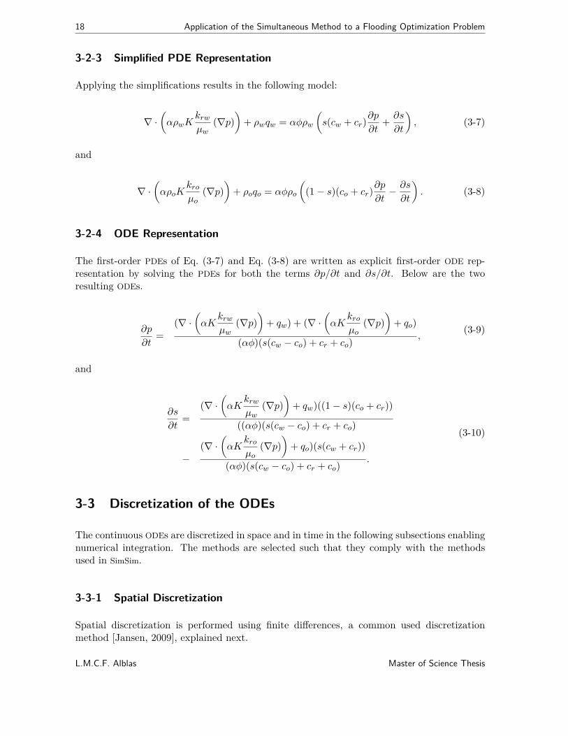
3-2-3 Simplified PDE Representation

Applying the simplifications results in the following model:

∇ ·(

αρwKkrw

µw(∇p)

)

+ ρwqw = αφρw

(

s(cw + cr)∂p

∂t+

∂s

∂t

)

, (3-7)

and

∇ ·(

αρoKkro

µo(∇p)

)

+ ρoqo = αφρo

(

(1 − s)(co + cr)∂p

∂t− ∂s

∂t

)

. (3-8)

3-2-4 ODE Representation

The first-order PDEs of Eq. (3-7) and Eq. (3-8) are written as explicit first-order ODE rep-resentation by solving the PDEs for both the terms ∂p/∂t and ∂s/∂t. Below are the tworesulting ODEs.

∂p

∂t=

(∇ ·(

αKkrw

µw(∇p)

)

+ qw) + (∇ ·(

αKkro

µo(∇p)

)

+ qo)

(αφ)(s(cw − co) + cr + co),

(3-9)

and

∂s

∂t=

(∇ ·(

αKkrw

µw(∇p)

)

+ qw)((1 − s)(co + cr))

((αφ)(s(cw − co) + cr + co)

−(∇ ·

(

αKkro

µo(∇p)

)

+ qo)(s(cw + cr))

(αφ)(s(cw − co) + cr + co).

(3-10)

3-3 Discretization of the ODEs

The continuous ODEs are discretized in space and in time in the following subsections enablingnumerical integration. The methods are selected such that they comply with the methodsused in SimSim.

3-3-1 Spatial Discretization

Spatial discretization is performed using finite differences, a common used discretizationmethod [Jansen, 2009], explained next.


3-3 Discretization of the ODEs 19

Finite Difference Discretization

The discretization is explained using the mass-balance for the water-phase equations, but themethod applies to the oil-phase equations as well. Firstly, the part of the continuous ODEscontaining the difference operator ∇ is elaborated. As earlier stated, K is a 2 × 2 diagonalmatrix with the values kxx, kyy.

∇ ·(

Kkrw

µw(∇p)

)

=∂

∂x

(

kxxkrw

µw

(∂p

∂x

))

+∂

∂y

(

kyykrw

µw

(∂p

∂y

))

. (3-11)

Secondly, the continuous space is approximated in discrete space as:

∂

∂x

(

kxxkrw

µw

(∂p

∂x

))

+∂

∂y

(

kyykrw

µw

(∂p

∂y

))

≈

∆

∆x

(

kxxkrw

µw

(∆p

∆x

))

+∆

∆y

(

kyykrw

µw

(∆p

∆y

))

.

(3-12)

Finally, the discretization is done using equally spaced grid-blocks in both the x-direction andthe y-direction, using the central difference approximation. The central difference approxi-mation is a method to numerically calculate a discrete derivative:

∆f(x)

∆x=

(

f(x + 12∆x) − f(x)

)

−(

f(x) − f(x − 12∆x)

)

∆x, (3-13)

where f(x) and x are an arbitrary function and an arbitrary variable used for demonstration.Applying the central difference approximation to Eq. (3-12) yields:

([

kxxkrw

µw

]

i+ 1

2,j,n

([p]i+1,j,n − [p]i,j,n) −[

kxxkrw

µw

]

i− 1

2,j,n

([p]i,j,n − [p]i−1,j,n)

)

(∆x)2+

([

kyykrw

µw

]

i,j+ 1

2,n

([p]i,j+1,n − [p]i,j,n) −[

kyykrw

µw

]

i,j− 1

2,n

([p]i,j,n − [p]i,j−1,n)

)

(∆y)2.

(3-14)

The subscripts i, j, n refer to the discrete space (i, j) (Figure 3-1) at time-step n.

Implementation of the Discrete Permeabilities

The central difference approximation requires to calculate the permeabilities at the borderof two grid blocks. The calculation for both the rock and the relative permeabilities will beexplained.

Rock permeabilities are approximated using the harmonic average:



1,1

2,1

1,j

i,ji,1

1,2

Figure 3-1: Representation of a two dimensional reservoir model with i rows and j columns.

[kxx]i+ 1

2,j = 2

[kxx]i+1,j [kxx]i,j[kxx]i+1,j + [kxx]i,j

,

[kyy]i,j+ 1

2

= 2[kyy]i,j+1[kyy]i,j

[kyy]i,j + [kyy]i,j+1.

(3-15)

Relative permeabilities cannot be computed using the harmonic average. The relative perme-abilities depend on the saturation which is described by a non-linear hyperbolic PDE, whichcorresponds to a moving water front through the reservoir (Section C-2-2). The saturationfor a certain grid block may change very rapidly in time as the water front moves along thisgrid block. Using a harmonic average as in Eq. (3-15) for the relative permeabilities is forthis reason not correct and will give an incorrect result [Aziz and Settari, 1979, p.153]. Therelative permeabilities in a certain grid block will be based on the saturation of the flow intothe grid block. This can be implemented by using upstream weighting:

[krw]i+ 1

2,j,n =

{

[krw]i,j,n if [p]i,j,n ≥ [p]i+1,j,n

[krw]i+1,j,n if [p]i,j,n < [p]i+1,j,n.(3-16)

The relative permeabilities are based on a basic Corey model [Corey, 1954], which is presentedin Eq. (3-17) and describes the relative permeability as exponential function of the normalizedwater saturation [Swn]i,j,n.

[krw]i,j,n = k0rw[Sn]nw

i,j,n,

[kro]i,j,n = k0ro(1 − [Sn]i,j,n)no ,

(3-17)

where k0rw, k0

ro are the endpoint permeabilities and nw, no are called the Corey exponents.The normalized water saturation Swn is defined as function of the water saturation s.

[Swn]i,j,n ,[s]i,j,n − Swc

1 − Sor − Swc, with 0 ≥ Sn ≥ 1. (3-18)


3-3 Discretization of the ODEs 21

With Swn ∈ [0, 1], this implies s ∈ [Swc, 1 − Sor]. Swc is the connate water saturation andSor is the residual oil saturation. The connate water saturation and residual oil saturationdetermine the minimum and maximum value of the actual water saturation s.

Eq. (3-16) causes the model to be discontinuous. Discontinuous models cannot be optimizedusing the simultaneous method. The relative permeabilities will be fixed to maintain contin-uous model equations. The fixation will be based on the pressure-values of the IG to complywith the models as obtained from SimSim.

Combination of the Discrete Equations

The transition from the continuous ODEs into difference equations will be described. Thediscretization steps are explained using Eq. (3-12) ,Eq. (3-13) and Eq. (3-14). The perme-abilities used in the ODEs are described in discrete space by Eq. (3-15), Eq. (3-16), Eq. (3-17)and Eq. (3-18).

Using these equations, the term with the difference operators will be recovered in two stages,using the transmissibility term T and the volumetric flow rate U .

∇ ·(

αKkrw

µw

)

(∇p) + qw =

Tw︷︸︸︷

∇ ·(

αKkrw

µw

)(1

∆x+

1

∆y

)

∆p + qw

︸︷︷︸

Uw

(3-19)

First the transmissibility parameters will be explained by defining [Tw,1]i,j,n, [Tw,2]i,j,n, [Tw,3]i,j,n,[Tw,4]i,j,n. The parameter α is replaced according to Eq. (3-4) with h∆x∆y.

[Tw,1]i,j,n = [Tw]i+ 1

2,j =

2h

µw

∆y

∆x

[kxx]i+1,j [kxx]i,j[kxx]i+1,j + [kxx]i,j

[krw]i+1/2,j,n

[Tw,2]i,j,n = [Tw]i− 1

2,j =

2h

µw

∆y

∆x

[kxx]i−1,j [kxx]i,j[kxx]i−1,j + [kxx]i,j

[krw]i−1/2,j,n

[Tw,3]i,j,n = [Tw]i,j+ 1

2

=2h

µw

∆x

∆y

[kyy]i,j+1[kyy]i,j[kyy]i,j+1 + [kyy]i,j

[krw]i,j+1/2,n

[Tw,4]i,j,n = [Tw]i,j− 1

2

=2h

µw

∆x

∆y

[kyy]i,j−1[kyy]i,j[kyy]i,j−1 + [kyy]i,j

[krw]i,j−1/2,n

(3-20)

The transmissibility terms are multiplied by the pressure differences. This recovers the withthe geometry factor multiplied Darcy velocities, which creates the volumetric flow rate U . Ifa well is enclosed in a grid block, the volumetric flow rate q will be added to the equation ofthe total volumetric flow rate U .

[Uw]i,j,n = [Tw,1]i,j,n([p]i+1,j,n − [p]i,j,n) + [Tw,2]i,j,n([p]i−1,j,n − [p]i,j,n)

+ [Tw,3]i,j,n([p]i,j+1,n − [p]i,j,n) + [Tw,4]i,j,n([p]i,j−1,n − [p]i,j,n) + [qw]i,j,n.(3-21)

Note from Eq. (3-21) the fact that a flow into a grid block has a positive sign, where flow outof a grid block will have a negative sign. Production flow rates are therefore negative.



3-3-2 Difference Equation Representation

With above steps it is possible to write the set of continuous ODEs presented by Eq. (3-9)and Eq. (3-10) as set of difference equations:

[∆p

∆t

]

i,j,n=

([Uw]i,j,n) + ([Uo]i,j,n)

(h∆x∆y)[φ]i,j([s]i,j,n(cw − co) + cr + co)(3-22)

[∆s

∆t

]

i,j,n=

([Uw]i,j,n)((1 − [s]i,j,n)(co + cr)) − ([Uo]i,j,n)([s]i,j,n(cw + cr))

(h∆x∆y)[φ]i,j([s]i,j,n(cw − co) + cr + co)(3-23)

3-3-3 Time Discretization and Integration

The difference equations represented by Eq. (3-22) and Eq. (3-23) are used to obtain the state-profiles of p and s using the by Eq. (3-24) backward or implicit Euler integration method.This is explained in Section 2-3 and complies to the SimSim models.

[t]n = [t]n−1 + ∆t,

[p]i,j,n = [p]i,j,n−1 + ∆t

[∆p

∆t

]

i,j,n,

[s]i,j,n = [s]i,j,n−1 + ∆t

[∆s

∆t

]

i,j,n.

(3-24)

3-4 Optimization

This section will describe the objective function which needs to be maximized and the physicalconstraints and the boundary conditions to enforce a feasible solution.

3-4-1 Objective Function

Maximizing the yield of the reservoir is done by setting a profit for produced oil and a lossfor injected and produced water, which is used to calculate the net present value (NPV).The objective function ϕ presented by Eq. (3-25) is based on the function described in[Jansen et al., 2009] and expressed in US dollars (usd).

ϕ([qw,inj ]i,j,n, [qw,prod]i,j,n, [qo,prod]i,j,n) =

Nt∑

t=1

Ni∑

i=1

Nj∑

j=1

(

[qw,inj ]i,j,n · rw,inj + [qw,prod]i,j,n · rw,prod + [qo,prod]i,j,n · ro,prod

)

(1 + b)tt/τ∆tt

,(3-25)


3-4 Optimization 23

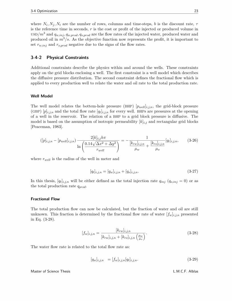
where Ni, Nj , Nt are the number of rows, columns and time-steps, b is the discount rate, τis the reference time in seconds, r is the cost or profit of the injected or produced volume inusd/m3 and qw,inj , qw,prod, qo,prod are the flow rates of the injected water, produced water andproduced oil in m3/s. As the objective function now represents the profit, it is important toset rw,inj and ro,prod negative due to the signs of the flow rates.

3-4-2 Physical Constraints

Additional constraints describe the physics within and around the wells. These constraintsapply on the grid blocks enclosing a well. The first constraint is a well model which describesthe diffusive pressure distribution. The second constraint defines the fractional flow which isapplied to every production well to relate the water and oil rate to the total production rate.

Well Model

The well model relates the bottem-hole pressure (BHP) [pwell]i,j,n, the grid-block pressure(GBP) [p]i,j,n and the total flow rate [qt]i,j,n for every well. BHPs are pressures at the openingof a well in the reservoir. The relation of a BHP to a grid block pressure is diffusive. Themodel is based on the assumption of isotropic permeability [k]i,j and rectangular grid blocks[Peaceman, 1983].

([p]i,j,n − [pwell]i,j,n)2[k]i,jhπ

ln

(

0.14√

∆x2 + ∆y2

rwell

) = − 1

[krw]i,j,n

µw+

[kro]i,j,n

µo

[qt]i,j,n, (3-26)

where rwell is the radius of the well in meter and

[qt]i,j,n = [qw]i,j,n + [qo]i,j,n. (3-27)

In this thesis, [qt]i,j,n will be either defined as the total injection rate qinj (qo,inj = 0) or asthe total production rate qprod.

Fractional Flow

The total production flow can now be calculated, but the fraction of water and oil are stillunknown. This fraction is determined by the fractional flow rate of water [fw]i,j,n presentedin Eq. (3-28).

[fw]i,j,n =[krw]i,j,n

[krw]i,j,n + [kro]i,j,n

(µw

µo

) . (3-28)

The water flow rate is related to the total flow rate as:

[qw]i,j,n = [fw]i,j,n[qt]i,j,n. (3-29)



3-4-3 Boundaries

A minimum number of variables needs to be bounded in order to satisfy the physical con-straints of the reservoir. This avoids the optimization algorithm to terminate in a non-physicaloptimum.

Saturations

The normalized water saturation Swn is bounded to Swn ∈ [0, 1]. Neglecting this bound wouldgenerate negative water saturations, leading to an infeasible and infinitely high oil production.

Well Pressures

The BHP of the well described by the pressure pwell is limited to avoid an infinite pressuredifference between the GBP p and the BHP pwell, what would result in an infinite flow rate aswell.

Flow Rates

To distinguish between an injection or a production well, the flow rates will be limited to beeither positive or negative respectively to avoid production wells turning into injection wellsand vice versa.

Flow at the Reservoir Boundaries

The reservoir is assumed to be a finite volume with no mass interaction with the surround-ings. This closed reservoir is obtained by influencing the transmissibilities at the reservoirboundaries where they are forced to be zero.

3-5 Concluding Remarks

It has been demonstrated how the simultaneous method can be applied to a flooding op-timization problem for a simplified reservoir model. Future work might include the use ofthree-dimensional models and include multiple phases. The steps of obtaining explicit first-order ODEs and applying a time-discretization would still hold for a three-phase model. Anadditional phase would result in an additional mass-balance and an additional state.

For compliance with SimSim as IG generator, the simulator which will be used for verificationand generation of the IGs, two implementation options have been adopted which might not bethe best choice in terms of optimization performance. The first is the problem of discontinuousbehavior of the relative permeabilities. The directions are now based on the pressure statesof the IG, which might result in a bad convergence behavior when the IG is selected lessoptimal. The second adoption is the use of the implicit Euler method for integration, whereorthogonal collocation could be used instead. This would results in a function approximationof the state-profiles, eliminating the need for direct integration as discussed in Section 2-3-1.


Chapter 4

Implementation of a Flooding

Optimization Problem in GAMS

The implementation of a flooding optimization problem using the simultaneous method isverified and tested to analyze its limitations. The limitations are explored by scaling up themodel and by selecting different values for the initial guess (IG). A flooding optimizationproblem is implemented in General Algebraic Modeling System (GAMS). GAMS is a softwarepackage based on algebraic modeling and is designed for solving optimization problems. Ithas the advantages of providing automatic discretization support and symbolic differentiation.State-of-the-art solvers can be selected for solving an optimization problem without the needfor adjusting the code. Compared to other software packages, solvers are better integrated inGAMS and GAMS can communicate with Matrix Laboratory (MatLab).

This chapter will first compare the GAMS implementation with a Simple Simulator (SimSim)model in order to verify the GAMS implementation in Section 4-1. Next, the optimizationperformance of four solvers will be described in Section 4-2, because they might give verydifferent results [Wächter and Biegler, 2006], [Poku and Biegler, 2004]. As the simultaneousmethod is known to be sensitive to IGs and given the fact that the size of the NLP may growrapidly [Biegler, 2007], both the feasibility of upscaling and the sensitivity to IGs are testedin Section 4-3 and Section 4-4 respectively. The chapter will be concluded in Section 4-5.

4-1 Model Verification

The GAMS model is verified using SimSim. SimSim is being developed by J.D. Jansen since2004 and used and improved since then. SimSim is based on the simplified PDEs presentedin Section 3-2 and is a matrix-oriented forward simulator using implicit Euler integration.It has also been compared to Modular Reservoir Simulator (MoReS), the in-house simulatorof Shell. Therefore, it is assumed SimSim provides representative and valid reservoir modelswhich can be used for model verification. The reservoir model used for verification is givenin Figure 4-1. The GAMS code is presented in Appendix D.


26 Implementation of a Flooding Optimization Problem in GAMS

i

j

1

2

31 2

Injection Well

Production Well

High Permeability

Medium Permeability

Low Permeability

Figure 4-1: Illustration of the reservoir model used for verification. The model consists of highpermeability fields (1e−12 m2), medium permeability fields (1e−13 m2) and a low permeabilityfield (1e−14 m2). One injection well is placed in grid block ((i, j) = (1, 1)) and one productionwell is placed in grid block ((i, j) = (2, 3)).

The verification is performed in two directions. Firstly, GAMS starts optimizing using flowrates, pressures and saturations obtained from a forward simulation in SimSim. GAMS startswith an initial error, which is a summation of the numerical errors and model differences.Secondly, after termination of the GAMS optimization, the resulting flow rates are used toperform a forward simulation in SimSim. The SimSim simulation is then compared with thevalues from GAMS for verification.

4-1-1 The Initial Error in GAMS due to the Initial Guess

The cause of the initial error is explained first, after which the origin of the error is discussed.

Cause of the Initial Error in GAMS

Every equation in GAMS is programmed once using spatial and time indexes (e.g. fi,j,n), afterwhich GAMS performs an automatic discretization in space and in time. The optimizationhorizon is 10 years, with a maximum time-step of 30 days, resulting in 123 time-steps. Soevery equation with spatial indexes i, j and time index n results in i · j · n = 2 · 3 · 123 = 738equations after automatic discretization. In total, the model consists of 13, 394 equations afterautomatic discretization. The equations are evaluated using the IG from SimSim. However,due to numerical or model errors the left-hand side may not be equal to the right-hand sideof these equations. The errors are added up for all 13, 394 equations, resulting in the initialerror.

Origin of the Initial Error in GAMS

GAMS initiates with an initial error in the order of 1e−1 due to errors in the implicit Eulerequations and the Peaceman well-model. The IG influences the initial error. For this reason,an IG has been selected which does not violate any constraints and which has only a smalldifference between the injection and production rates. The IG is for this reason based on aconstant injection rate of 0.0059 m3/s and a constant production rate of −0.0061 m3/s.


4-1 Model Verification 27

It has been investigated which relative errors are the largest. The relative errors are calculatedusing the absolute error of the equation divided by the order of magnitude of the equation.The highest relative error is selected. This is summarized in Table 4-1.

Equation Order of Relative Error

Peaceman Well Model 1e+02%Implicit Euler Saturation 1e−03%Implicit Euler Pressure 1e−08%

Table 4-1: A presentation of the maximum relative initial errors in GAMS. The maximum relativeerrors are calculated using the maximum absolute error of the equation divided by the order ofmagnitude of the equation. The absolute errors are based on the summation of the errors due todifferences in the left-hand side and right-hand side of the in GAMS discretized equations. Thehighest relative error is presented. A relative error in the order of 1e+02% for the Peacemanequation implies that one side of the equation may be a multiple of the other side.

A relative error in the order of 1e+02% implies that one side of the equation may be amultiple of the other side. Evaluation of the error for every single Peaceman equation revealsthe error to be present from time-step n > 95. This appears to be the point where waterbreaks through. The Peaceman well model has been compared to SimSim and both modelsare identical. All three major errors are reproducible and therefore not due to the limit ofcomputational precision. Increasing the time horizon does not increase the maximum relativeerror.

4-1-2 Comparison of GAMS with the Forward Simulator SimSim

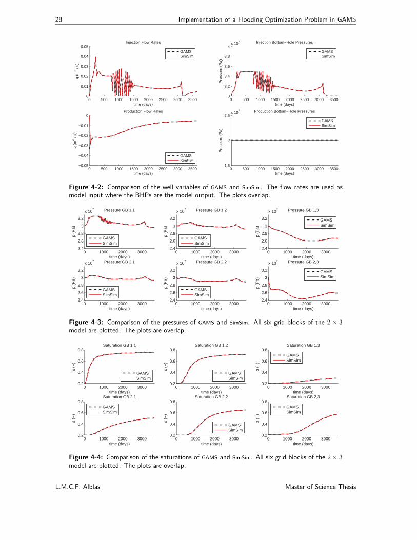
The results of GAMS are compared to the results of SimSim. The results of SimSim are basedon the flow rates of a GAMS optimization. Selecting flow rates as input will result in the BHPsas output. The BHPs have therefore the largest error. The time profiles of the well variables,pressures and saturations are presented in Figure 4-2 , Figure 4-3 and Figure 4-4.

Both models are using an equal time-step discretization of maximum 30 days, which is de-termined by SimSim. In total, 123 time-steps are used to simulate the forward model for aoptimization horizon of 10 years. The fluctuations of BHP are limited to [+50e5, 0] Pa and[0, −100e5] Pa. Although a fluctuation in BHP of −50e5 Pa may be more realistic, a bound of−100e5 Pa is selected to allow for an IG based on a production rate of −0.0061 m3/s withoutviolation of any boundaries. The boundaries in GAMS are not implemented in SimSim, thoughthey are still satisfied.

Both models behave similar. The error in terms of percentage has been calculated for time-steps n = 2, 3, ..., N . The first time-step is left out because the first time-step is not correctlycalculated by SimSim. For example, BHPs at time-step n = 1 are zero where they shouldbe equal to the reservoir pressure. All the values for the error in terms of percentage arepresented in Table 4-2. Although the models behave similar, small differences are present.It is clear well rates are used as simulation input. The highest error is not more than 0.5%.Using a time-horizon of 40 years does not change the maximum error in terms of percentage.



0 500 1000 1500 2000 2500 3000 35000

0.01

0.02

0.03

0.04

0.05Injection Flow Rates

time (days)

q (m

3 / s)

GAMSSimSim

0 500 1000 1500 2000 2500 3000 3500−0.05

−0.04

−0.03

−0.02

−0.01

0Production Flow Rates

time (days)

q (m

3 / s)

GAMSSimSim

0 500 1000 1500 2000 2500 3000 35003

3.2

3.4

3.6

3.8

4x 10

7 Injection Bottom−Hole Pressures

time (days)

Pre

ssur

e (P

a)

GAMSSimSim

0 500 1000 1500 2000 2500 3000 35001.5

2

2.5x 10

7 Production Bottom−Hole Pressures

time (days)

Pre

ssur

e (P

a)

GAMSSimSim

Figure 4-2: Comparison of the well variables of GAMS and SimSim. The flow rates are used asmodel input where the BHPs are the model output. The plots overlap.

0 1000 2000 30002.4

2.6

2.8

3

3.2

x 107 Pressure GB 1,1

time (days)

p (P

a)

GAMSSimSim

0 1000 2000 30002.4

2.6

2.8

3

3.2


time (days)

p (P

a)

GAMSSimSim

0 1000 2000 30002.4

2.6

2.8

3

3.2


time (days)p

(Pa)

GAMSSimSim

0 1000 2000 30002.4

2.6

2.8

3

3.2


time (days)

p (P

a)

GAMSSimSim

0 1000 2000 30002.4

2.6

2.8

3

3.2


time (days)

p (P

a)

GAMSSimSim

0 1000 2000 30002.4

2.6

2.8

3

3.2


time (days)

p (P

a)

GAMSSimSim

Figure 4-3: Comparison of the pressures of GAMS and SimSim. All six grid blocks of the 2 × 3model are plotted. The plots are overlap.

0 1000 2000 30000.2

0.4

0.6

0.8Saturation GB 1,1

time (days)

s (−

)

GAMSSimSim

0 1000 2000 30000.2

0.4

0.6


time (days)

s (−

)

GAMSSimSim

0 1000 2000 30000.2

0.4

0.6


time (days)

s (−

)

GAMSSimSim

0 1000 2000 30000.2

0.4

0.6


time (days)

s (−

)

GAMSSimSim

0 1000 2000 30000.2

0.4

0.6


time (days)

s (−

)

GAMSSimSim

0 1000 2000 30000.2

0.4

0.6


time (days)

s (−

)

GAMSSimSim

Figure 4-4: Comparison of the saturations of GAMS and SimSim. All six grid blocks of the 2 × 3model are plotted. The plots are overlap.


4-2 Selection of the Best Performing Solver 29

Variable Error (%) Variable Error (%)

[p]1,1,n 1.4e−02 [s]1,1,n 2.1e−08[p]1,2,n 5.7e−03 [s]1,2,n 4.2e−04[p]1,3,n 5.5e−04 [s]1,3,n 1.8e−03[p]2,1,n 4.5e−07 [s]2,1,n 5.0e−01[p]2,2,n 4.5e−07 [s]2,2,n 6.9e−02[p]2,3,n 5.1e−08 [s]2,3,n 1.4e−02

[qw]1,1,n 0.0e+00 [qw]2,3,n 6.2e−02[qo]1,1,n 0.0e+00 [qo]2,3,n 2.0e−07[pwell]1,1,n 1.4e−02 [pwell]2,3,n 7.0e−07

Table 4-2: The maximum error in terms of percentage calculated for all states, inputs andoutputs of GAMS and SimSim. The well rates of GAMS are used by SimSim to perform a forwardsimulation. The highest error is not more than 0.5%.

4-2 Selection of the Best Performing Solver

Solvers may perform very different depending on the optimization problem, as can be foundin for example [Wächter and Biegler, 2006] and [Poku and Biegler, 2004]. It is therefore in-vestigated which solvers perform the best when applied to a flooding optimization problem.Multiple solvers have been applied to flooding optimization problems, of which the four mostpromising solvers are selected. The selected solvers will be described first after which theresults will be compared on the obtained NPV, optimization time and behavior.

4-2-1 Description of Different Solvers

Four selected solvers are described. They all exploit the sparsity of the NLP and approxi-mate the second-order derivative information based on the algebraically calculated first-ordergradient.

CONOPT 3.0

CONOPT is introduced by [Drud, 1985] and uses a generalized reduced gradient (GRG) al-gorithm. A GRG algorithm basically takes an iteration-step along its vertices, where thevertices are the boundaries of the search-space, for example equality constraints or active in-equality constraints, better known as active sets. Unbounded variables, also called super-basicvariables, are then used to minimize the optimization problem. According to the article of[Biegler and Grossmann, 2004], GRG methods are the most poplar among all gradient basedNLP solvers.

CONOPT can handle up to 4000 equations [Drud, 1994]. More recent publications are notavailable, but according to [Mittelmann, 2010] the solver will still be able to handle 1e5decision variables.

IPOPT 3.8



IPOPT is initiated by [Wächter, 2002] and uses an interior point (IP) algorithm. An IP algo-rithm basically adds constraints to the objective function using barrier functions. A barrierfunction is zero when the constraint is satisfied, but will go to infinity along a smooth pathwhen a constraint is violated. According to [Biegler and Grossmann, 2004], IPOPT can solveproblems up to 1e6 variables on a high-end personal computer.

KNITRO 6.0

KNITRO is initially introduced as an IP solver. In a later stage it has been extended with asecond IP solver and with an sequential linear programming (SLP) algorithm using active sets.This SLP algorithm can be interpreted as a GRG algorithm on a linearized problem. This isused to improve the robustness in convergence, where the SLP algorithm is also used effectivelyto determine active constraints [Byrd et al., 2006]. KNITRO shows to be very effective withmany active constraints [Gould et al., 2005].

From [Mittelmann, 2010], and according to [F. Cadoux] of the company Artelys and theKNITRO website1, it shows that KNITRO should be capable of problems in the order of 1e6variables and constraints on a high-end personal computer.

SNOPT 6.0

SNOPT uses a sparse sequential quadratic programming (SQP) algorithm [Gill et al., 2002]with an approximated Hessian. An SQP algorithm adds the constraints to the objectivefunction and uses a second-order Taylor polynomial as minimization function. SNOPT isrelatively efficient if the number of degrees of freedom (DOF) is small. Compared to othersolvers, SNOPT requires few function evaluations due to the quadratic approximation of theLagrange function.

According to the articles of [Gill et al., 2002] and [Mittelmann, 2010] SNOPT can handle upto 1e5 variables.

4-2-2 Comparison of Different Solvers

CONOPT, IPOPT and SNOPT might be able to obtain a local optimum when applied to aflooding optimization problem. KNITRO and all other NLP solvers which come with GAMS

were not able to solve a flooding optimization problem, resulting in an infeasible termination.The solvers are compared using the reservoir model presented in Figure 4-1. The IG is basedon a constant injection rate of 0.0059 m3/s and a constant production rate of −0.0061 m3/s.These settings give typical results which are also obtained using smaller models or differentIGs.

The results are presented in Table 4-3, where the solvers are compared on the obtained NPV

and the optimization time. SNOPT will only obtain a feasible solution, but does not optimizethe problem. IPOPT is almost two times faster than CONOPT, but the NPV found by CONOPT

is significantly higher compared to other solvers. KNITRO terminates infeasible. Solvers come


4-2 Selection of the Best Performing Solver 31

Solver NPV Optimization Time(usd) (s)

Initial Guess 3.84e8 not applicable

CONOPT 8.16e8 50.5IPOPT 5.57e8 27.8KNITRO infeasible > 1800SNOPT 3.84e8 2.9

Table 4-3: Presentation of four GAMS solvers compared to the IG. The performance is comparedon the obtained NPV and the required optimization time. Using CONOPT results in the highestNPV. SNOPT is the fastest, but does not optimize the problem. IPOPT is faster than CONOPT butdoes not obtain the highest NPV. KNITRO terminates infeasible.

with option files which can be tweaked to improve the performance. This has been done forCONOPT described in Section D-3.

The resulting profiles of the well variables are presented in Figure 4-5. Although CONOPT

provides the highest NPV, the output is the most chattering as well. It has been tried to usetwo solvers successively, which did neither improve the NPV nor the required optimizationtime nor the output behavior.

0 500 1000 1500 2000 2500 3000 3500

0

0.01

0.02

0.03


time (days)

q (m

3 / s)

IG SimSimCONOPTIPOPTKNITROSNOPT

0 500 1000 1500 2000 2500 3000 3500−0.04

−0.03

−0.02

−0.01


time (days)

q (m

3 / s)


0 500 1000 1500 2000 2500 3000 3500

3

3.2

3.4

3.6

3.8

x 107 Injection Bottom−Hole Pressures

time (days)

Pre

ssur

e (P

a)


0 500 1000 1500 2000 2500 3000 35001.8

2

2.2

2.4

2.6

2.8

3x 10


time (days)

Pre

ssur

e (P

a)

Figure 4-5: Presentation of four GAMS solvers compared to the initial guess. The performanceis compared on resulting behavior of the optimal solution. CONOPT gives the most chatteringbehavior.

1http://www.ziena.com/papers/case_performance.pdf



4-3 Scaling

Compared to the sequential method, the simultaneous method generates a very large non-linear programming (NLP) problem due to the spatial and time discretization for all variablesand states. This section will be used to demonstrate the size of the NLP problem as well asto discover whether the current implementation can be used for larger models.

A 2 × 2 model with a homogeneous rock permeability of 1e−13 m2 and square grid blocksis used initially. The decision for such a model is based on the fact that SimSim cannot dealwith smaller models and cannot deal with non-square grid blocks. The model has an injectorin the top-left corner and a producer in the bottom-right corner. The rock permeability isthe logarithmic average of the model used for verification. The optimizations are initiatedwith an IG based on a constant injection rate of 0.006 m3/s and a constant production rateof −0.0065 m3/s. The upscaling will be done by adding an additional column of two verticalgrid blocks in between the wells as illustrated in Figure 4-6.

i

j

1

2

1 2

j

31 2

Injection Well

Production Well

Figure 4-6: Illustration of a first step in upscaling; Grid blocks will be added as a column inbetween the columns containing the wells. The injection well will be placed in the top-left cornerand the production well will be placed in the bottom-right corner.

The upscaling will change the model properties due to the displacement of the wells and thesize of the model in terms of cubic meters. Therefore the net present value (NPV) of thedifferent models is not compared. A better approach would be to refine the grid blocks bydividing every grid block in nine smaller grid blocks. This would keep the model propertiesidentical. However, the current implementation of the simultaneous method is not yet ableto solve these larger models. For this reason, the upscaling of the model is limited to smallproblems.

The optimizations are executed on a standard desktop computer with a 2.8 ghz processorand 4 gb of memory running at a 64-bit Windows operating system. 30 test cases have beenoptimized for different IGs, of which 6 are presented in Table 4-4 to demonstrate the increasein the number of variables and optimization time when scaling up the model. Models of2 × 5 grid blocks could only be solved incidentally depending on the time-horizon. Models of2 × 6 grid blocks and larger have been tried to optimize as well, but conopt was not able toproduce feasible solutions.

Comparing cases 3 and 4 of Table 4-4, the optimization horizon quadruples, while the op-timization time increases with more than a factor 18. This behavior is similar for cases (1and 2) and (5 and 6). The optimization horizons are different, because models may become


4-4 Sensitivity to Initial Guesses 33

Case Ni Nj Nt Horizon No. Variables Optimization Time Initial Error(-) (-) (-) (years) (-) (s) (-)

1 2 2 123 10 9,516 3.9 0.302 2 2 243 20 18, 984 25.9 2.293 2 3 123 10 13,777 10.3 0.734 2 3 487 40 54, 545 189.1 6.125 2 4 123 10 17,959 53.1 9.886 2 4 609 50 88, 915 2746.5 17.51

Table 4-4: Comparison of six optimizations which differ in model size (Ni ·Nj) and in the numberof time steps (Nt), resulting in a different optimization horizon due to a constant time-step. Themodels are compared on the number of variables, the required optimization time and the initialerror. For every model size, two time-horizons were selected. The horizons differ because someoptimizations terminated infeasible. The bold optimizations have identical optimization horizonsand can therefore be compared on the effect of upscaling the model in terms of the number ofgrid blocks. The optimizations are initiated with an IG based on a constant injection rate of0.006 m3/s and a constant production rate of −0.0065 m3/s.

infeasible for specific horizons. Besides an increase in the number of time steps, an increasein the number of model grid blocks is of significant influence on the optimization time as well.Comparing cases 1 and 5, the number of grid blocks doubles while the optimization timeincreases with a factor 13.6. It can be computed that the number of variables is almost linearto the number of grid blocks multiplied by the number of time steps. On the 30 test-cases,the average number of decision variables is close to 18 variables per grid block per time-step.

It must be noted that the number of decision variables is not a hard number, as auxiliaryvariables are counted as well. However, the number is a measure of the size of the NLP

problem. Note the difference in NLP size compared to the sequential method, where the NLP

of cases 1, 3 and 5 would consist of 2 wells · 123 time-steps or 246 variables, independent ofthe number of grid blocks.

Tests have also been performed to investigate the influence of the selected rock permeability.A model with 2 × 8 grid blocks and 246 time-steps with a rock permeability of 1e−12 m2 hasbeen solved in 702.5 s. Decreasing the permeability to values of 1e−14 m2 has the oppositeeffect resulting in less feasible solutions. Again, the number of variables and the numberof grid blocks are not a hard indication and dependent on the model parameters, but theydemonstrate the problems of upscaling due to use of the simultaneous method.

4-4 Sensitivity to Initial Guesses

An IG provides initial values for all decision variables of an NLP problem. The IG mayinfluence the optimization performance and optimal objective value as it can be difficult tofind suitable values for all states for the complete time-horizon ([Cuthrell and Biegler, 1987],[Poku and Biegler, 2004]), as they must satisfy all constraints.

For this reason it is investigated what the impact of different IGs is on the NPV and theoptimization time. The model presented in Figure 4-1 is used. The IGs are generated bySimSim and based on continuous injection and production rates. The time horizon is 10 years



divided in 123 time-steps of 30 days. The optimization has injection and production bottem-hole pressure (BHP) constraints of +50e5 Pa and −100e5 Pa. Injection rates are positive andproduction rates are negative.

4-4-1 Sensitivity Measure to Different Initial Guesses

58 different IGs are tested which are based on flow rates of which the absolute productionrate is higher than the injection rate. Or, qinj + qprod < 0. The IGs are based on flow ratesbetween 1e−1 m3/s and 1e−5 m3/s. For reference, an optimized flow rate will be in the orderof 1e−2 m3/s. The IGs are compared on NPV, optimization time and other observations asthe initial error in GAMS and the initial violation of constraints.

Net Present Value

From the 58 optimizations, 43 terminated locally optimal and 15 terminated infeasible. 22of the 43 local optimal solutions terminated with an NPV which do not differ more than 1%from the highest obtained NPV. The 20 highest NPVs do not differ more than 0.08%. It hasbeen investigated what the initial NPV has been for the best performing optimizations, andfor every optimization the initial NPV was less than the optimized NPV. The smallest initialerrors did not give the best optimization performance neither in terms of NPV nor in termsof time. The IGs from 8 of the 22 optimizations with the highest NPV did violate the BHP

constraints.

The absolute differences between the injection and production flow rates from the 22 bestperforming optimizations in terms of NPV where less then 0.005 m3/s. The production ratewas never more than twice the injection rate. However, the injection and production ratesdid vary between values from 1e−2 m3/s to 1e−5 m3/s.

Optimization Time

The optimization times varied between several seconds to minutes. From the 10 fastest opti-mizations which terminated locally optimal, only 3 were also one of the ten highest obtainedNPVs. The 10 best performing optimizations in terms of time all violated the BHP constraints,where some BHPs were even zero over a period of multiple time-steps.

Observations

Several IGs are presented in a plot to observe whether the best IGs resulting in the highestNPVs do have similar dynamics compared to the optimized well variables. In terms of theresulting NPV of the optimization, the best 7 (optimal), the worst 5 (feasible) and 4 infeasibleIGs are plotted in Figure 4-7 and Figure 4-8. This is done for the grid block with the injectionwell, because this grid block is the first to show changes in the states. The pressures of the IGsresulting in the highest NPV all show an initial increase to a value above 300e5Pa, however,it is not a guarantee for an optimal solution as also infeasible IGs may have such a profile.For the saturations the profile of the optimal IGs do not follow a clear path.


4-4 Sensitivity to Initial Guesses 35

0 500 1000 1500 2000 2500 3000 35002.4

2.6

2.8

3

3.2

3.4

3.6x 10

7 Injector Grid Block Pressure

time (days)

p (P

a)

OptimizedIG with Optimal ResultIG with Feasible ResultIG with Infeasible Result

0 100 200 300 400 5002.98

2.99

3

3.01

3.02

3.03

3.04

3.05x 10

7 Injector Grid Block Pressure − Zoomed In

time (days)

p (P

a)


Figure 4-7: In terms of the resulting NPV after optimization, the best 7 (optimal), the worst5 (feasible) and 4 infeasible IGs are plotted. The left graph shows the pressure for the fulloptimization horizon, where the right graph is zoomed in on the first 500 days, indicated in theleft graph with a box. There is no clear distinction between the optimal, feasible and infeasibleIGs.

0 500 1000 1500 2000 2500 3000 35000

0.1

0.2

0.3

0.4

0.5

0.6

0.7

0.8

0.9

1Injector Grid Block Saturation

time (days)

s (−

)


0 100 200 300 400 5000.2

0.205

0.21

0.215

0.22

0.225

0.23

0.235

0.24

0.245

0.25Injector Grid Block Saturation − Zoomed In

time (days)

s (−

)


Figure 4-8: In terms of the resulting NPV after optimization, the best 7 (optimal), the worst5 (feasible) and 4 infeasible IGs are plotted. The left graph shows the saturation for the fulloptimization horizon, where the right graph is zoomed in on the first 500 days, indicated in theleft graph with a box. There is no clear distinction between the optimal, feasible and infeasibleIGs.



4-4-2 Sensitivity to Ill-Conditoned Initial Guesses

Other IGs have also been tried, based on the following criteria:

1. Contra-intuitive flow rates; qinj + qprod > 0, creating a lower production rate thaninjection rate.

2. No activity; qinj = qprod = 0.

3. Elimination of flow rates in the pressure ordinary differential equation (ODE) (Eq. (3-9))is known to cause singularities; choosing qw + qo = 0 can be achieved by choosingqinj + qprod = 0 as the production of water is initially very small relative to the oilproduction.

4. No IG; so all variables are set to zero initially.

Selecting IGs based on contra-intuitive flow rates or zero flow rates resulted in an infeasibletermination of the optimization. No IG lead to an infeasible solution as well. However,choosing the IGs such that the flow rates cancel out did provide comparable results as wherethe IGs were based on higher production rates than injection rates.

As indicated in Section 3-5, the relative permeabilities are fixed to enable continuous modeling.The influence of optimal solutions has been investigated and the changed flow directions areless than 2%. The change in the transmissibility term may be significant, as this terms isdirectly dependent on the relative permeability, which can change from grid block to gridblock up to a factor 25.


The GAMS model has been verified with SimSim and four solvers have been compared. Analysisshowed that the implementation of the current simultaneous method terminates infeasiblewhen scaled up and that it is sensitive to IGs.

GAMS supports automatic discretization and calculates gradient information symbolically. Arelative large initial error is caused by the equations of the Peaceman well model. Nonethelessthe well models used in both equations are similar. Comparing the GAMS results in SimSim

shows the error to be maximum 0.5%. Every optimization run produces an identical error.This indicates that the error is not due to computational limitations, but due to implementa-tion differences. The differences are caused by distinct modeling environments, where SimSim

is matrix-oriented and GAMS is equation-oriented.

The behavior of the optimal state-profiles can be physically interpreted. As much as possibleoil is pushed out of the reservoir, after which the injection rate is relaxed in order to let waterflow into the less permeable grid blocks. In the end, more water is injected to enable to pushout the last oil. The hyperbolic behavior of the saturations is encountered as explained inSection C-2-2.

conopt gives the best performance in terms of NPV. Although conopt is not the fastestsolver, the NPV is significantly higher compared to ipopt and snopt. Other solvers terminate


4-5 Concluding Remarks 37

infeasible, this points to either an ill-conditioned optimization problem or indicates that theother solvers cannot be applied to this type of optimization problem. An ill-conditionedproblem is a problem which does not have a unique optimal solution or which is discontinuous.In this case a non-unique or weak solution exists.

Upscaling of the model is limited to 16 grid blocks or 88,915 decision variables. Increasing thenumber of variables will enhance the chance of the optimization to terminate infeasible. Thecomputer is not running out of memory, indicating the infeasibilities are likely to be due tothe fact the optimization problem is ill-conditioned, the IG generator is not good enough orthat conopt cannot deal with larger models. As described in Section 4-2, the simultaneousmethod has been applied to problems in the order of 1e6 variables. This indicates thereshould still be room for improvement.

IGs based on constant injection and production rates showed to have significant influenceon the outcome of the simultaneous method. Only 22 of the 58 optimizations obtained itsmaximum within a bound of 1% of the highest NPV. The high sensitivity can be either causedby large model differences or it can be due to a weak solution, because the 20 highest NPVsdiffer less than 0.08%

To emphasize the relevance of the next chapter, it is observed that a chattering injectionflow rate influences the pressure of the injection grid block. However, the chattering signalvanishes over space and completely disappears in the producing grid block. The pressuredistribution is diffusive as described in Section C-2-1. Together with the fact none of theNPVs are identical, this indicates the existence of a weak solution.




Chapter 5

Comparison of the Simultaneous

Method and the Sequential Method

This chapter will compare the simultaneous method with the sequential method with respectto dealing with state-constraints in Section 5-1 and multi-objective optimization in Section 5-2.Section 5-3 compares both optimizations of the sequential method and the simultaneousmethod on the obtained optimal well-variable profiles. The sequential optimization will beperformed using Modular Reservoir Simulator (MoReS), the in-house reservoir simulator ofShell. Finally, Section 5-4 will end the chapter with concluding remarks.

5-1 Applying State-Constraints

One of the main issues of the currently used sequential method is the limited ability to dealwith state-constraints [Kraaijevanger et al., 2007]. The simultaneous method should providean advantage, which will be tested. The reservoir model has two types of states, pressuresand saturations. The pressure constraints are always present in practice [Sarma et al., 2006].Saturations are already bounded as explained in Section 3-4-3 for implementation reasons.For this reason, only pressure constraints are applied. The constraints are applied on a singlegrid block and on the whole reservoir.

5-1-1 Single Pressure Constraint

A single pressure constraint is applied on grid block (i, j) = (1, 2). As can be seen in Fig-ure 4-4, most of the water flows through this grid block due to the high permeability. Thepressure constraint is set to [p]1,2,n ∈ [299e5, 301e5]. The initial guess (IG) is based on aconstant injection rate of 0.0059 m3/s and a constant production rate of −0.0061 m3/s.

The simultaneous method is able to deal with the state-constraint. The net present value(NPV) changes from 8.155e8 usd to 8.134e8 usd, which is a change of less than −0.27%. It


40 Comparison of the Simultaneous Method and the Sequential Method

0 500 1000 1500 2000 2500 3000 35002.9

2.92

2.94

2.96

2.98

3

3.02

3.04

3.06

3.08

3.1x 10

7 Pressure GB 1,2

time (days)

p (P

a)

ConstrainedUnconstrainedBoundaries

Figure 5-1: Pressure in grid block (i, j) = (1, 2) for a constrained ([p]1,2,n ∈ [299e5, 301e5])and unconstrained optimization.

has also been investigated and confirmed that the simultaneous method is able to deal withstate-constraints at single points in time.

5-1-2 Reservoir Pressure Constraint

The reservoir pressure is constrained to [p]i,j,n ∈ [295e5, 305e5] as presented in Figure 5-2.The IG have been adjusted and multiplied by 1e−1 to avoid having an infeasible IG violatingthe pressure constraints. The IG is for this reason based on a constant injection rate of0.00059 m3/s and a constant production rate of −0.00061 m3/s.

From Figure 5-2 it can be observed all the constraints are satisfied. The optimum however isaffected and equal to 2.132e8 usd. The chattering disappears.

5-2 Multi-Objective Optimization

A multi-objective optimization is difficult to implement in the sequential method as it re-quires a combination of input, output and state constraints. This has been encounteredby [van Essen et al., 2010], in which a multi-objective optimization shows to be computa-tionally expensive. The chattering behavior of the solution demonstrated in Figure 4-2and Figure 4-3 is also mentioned in [Jansen et al., 2009]. Both [van Essen et al., 2010] and[Jansen et al., 2009] recognize the existence of a weak solution. An indication for a weak so-lutions is described in Section 4-4, where different values for the NPV are found. However, thehighest 20 NPVs do not differ more than 0.08%. The existence of a weak solution indicatesan under-constrained problem. The remaining degrees of freedom (DOF) can for examplebe used to minimize the variance of the solution. This can be done in two ways. The firstmethod is to optimize the problem by adding the variance as cost to the objective function,called regularization. The second method is called lexicographic optimization and bounds theoptimal NPV after which a variance minimization is performed. The variance of the inputs


5-2 Multi-Objective Optimization 41

0 1000 2000 30002.4

2.6

2.8

3

3.2

3.4

3.6x 10

7 Pressure GB 1,1

time (days)

p (P

a)


0 1000 2000 30002.4

2.6

2.8

3

3.2

3.4

3.6x 10

7 Pressure GB 1,2

time (days)

p (P

a)


0 1000 2000 30002.4

2.6

2.8

3

3.2

3.4

3.6x 10

7 Pressure GB 1,3

time (days)

p (P

a)


0 1000 2000 30002.4

2.6

2.8

3

3.2

3.4

3.6x 10

7 Pressure GB 2,1

time (days)

p (P

a)


0 1000 2000 30002.4

2.6

2.8

3

3.2

3.4

3.6x 10

7 Pressure GB 2,2

time (days)

p (P

a)


0 1000 2000 30002.4

2.6

2.8

3

3.2

3.4

3.6x 10

7 Pressure GB 2,3

time (days)

p (P

a)


Figure 5-2: The reservoir model pressures for a constrained ([p]i,j,n ∈ [295e5, 305e5]) andunconstrained optimization.

is described using a quadratic convex function often used in model predictive control (MPC)[Qin and Badgwell, 2003]. This is done using the Euclidean norm with a finite time-horizon,presented by Eq. (5-1).

Jvar = −Nt−1∑

n=1

[

[ww]n(

[qw]i,j,n − [qw]i,j,n+1

)2+ [wo]n

(

[qo]i,j,n − [qo]i,j,n+1

)2]

, (5-1)

where Jvar is the additional objective representing the variance of the weighted flow rateswith the weightings [ww]n, [wo]n. The term above is a sum of convex functions and thereforeconvex as well. The term has to be negative since a maximization is performed instead of aminimization.

5-2-1 Regularization

The regularized optimization is executed by adding the term of Eq. (5-1) to the NPV presentedby Eq. (3-25). Eleven regularized optimizations are compared to a standard or non-regularizedoptimization.

For the 11 best performing IGs in terms of NPV obtained in Section 4-4, the final NPV showed tobe affected less than 0.06%. For the weighting values are selected such that the smootheningis in the order 1e−2 of the NPV, putting the weighting on optimization of the NPV. This



0 500 1000 1500 2000 2500 3000 35000

0.01

0.02

0.03

0.04


time (days)

q (m

3 / s)

RegularizedNon−Regularized

0 500 1000 1500 2000 2500 3000 3500−0.05

−0.04

−0.03

−0.02

−0.01

0Flow Rates

time (days)

q (m

3 / s)


0 500 1000 1500 2000 2500 3000 35002.8

3

3.2

3.4

3.6x 10

7 Bottom−Hole Pressures

time (days)

Pre

ssur

e (P

a)


0 500 1000 1500 2000 2500 3000 35001.5

2

2.5x 10

7 Bottom−Hole Pressures

time (days)

Pre

ssur

e (P

a)


Figure 5-3: Regularized optimization compared to a non-regularized optimization. The wellvariables of the regularized optimization are smooth with a loss in NPV of less than 0.06%.

resulted in [ww]n = [wo]n = 1e10. Tuning the weighting may be a difficult procedure as theweighting influences the value of the variance. The difference in optimization time has alsobeen compared and is summarized in Table 5-1. The optimization time of the regularizedoptimization compared to non-regularized optimization may be significant. Chattering iseliminated as shown in Figure 5-3. The optimal solution becomes non-singular and thereforeunique or non-weak. This is also described in the paper of [Jacobson et al., 1970].

Change in Optimization Time

Median +19%Mean +23%Minimum −45%Maximum +125%

Table 5-1: Time performance of a regularized optimization compared to a non-regularized op-timization based on 11 optimizations. A regularized optimization can improve the optimizationtime, but may take on average 23% more time.

It has also been tried to increase the weighting of the smoothening function drastically, afterwhich the influence would slowly diminish. However, this resulted in an NPV of < 50% of thenon-regularized NPV. The values of the NPV for the regularized optimizations were 8 out of 11times identical where they were all different for non-regularized optimizations. The variancedecreases with a factor in the order of 1e2.

5-2-2 Lexicographic Optimization

The lexicographic optimization method first optimizes the NPV, after which the NPV isbounded and a variance minimization is performed. This method is a more convenient way to


5-3 Comparison with the Sequential Optimization Method 43

minimize variance, as the influence of the variance minimization can be controlled very wellby bounding the NPV.

Different lower-bounds have been implemented on the NPV. The bounds on the NPV werealways satisfied during the 11 test-cases. The results of lexicographic optimization are verysimilar to regularized optimization as presented in Figure 5-3.

To compare the lexicographic method with the regularized method, the lower bound is set toϕmin = ϕ−5e5 usd. This results in a change in the value of the objective function of < 0.06%which has also been encountered in the regularized optimization. The results in optimizationtime are presented in Table 5-2.

Change in Optimization Time

Median +52%Mean +66%Minimum +32%Maximum +152%

Table 5-2: Time performance of a lexicographic optimization compared to a basic optimizationbased on 11 optimizations. A lexicographic optimization may take on average 66% more time.

The optimization takes on average 66% more time which is significant and more compared toa regularized optimization, where the average additional time is 23%.

5-3 Comparison with the Sequential Optimization Method

This section will compare the simultaneous method with the sequential method. MoReS, thein-house simulator of Shell, is used for the sequential optimizations. Two optimizations willbe performed, of which Case 1 has only maximum injection and production constraints onthe bottem-hole pressure (BHP), where the optimization of Case 2 also has constraints on theflow rates, presented in Table 5-3.

Case 1 Case 2

qinj,IG 0.0059 m3/s 0.01 m3/sqprod,IG −0.0061 m3/s −0.012 m3/s

qinj,max n.a. 0.01 m3/sqprod,min n.a. −0.012 m3/spinj,max 350e5 Pa 350e5 Papprod,min 200e5 Pa 200e5 Pa

Table 5-3: IGs and constraints for two test-cases which will be used to compare the simultaneousmethod with the sequential method.

In the first subsection, a comparison will be made between the models of MoReS and Sim-ple Simulator (SimSim) by comparing the IGs used for optimizations in MoReS and GeneralAlgebraic Modeling System (GAMS). The results of these optimizations are presented in thesecond subsection.



0 500 1000 1500 2000 2500 3000 35000

0.005

0.01


time (days)

q (m

3 / s)

MoReSSimSim

0 500 1000 1500 2000 2500 3000 3500−0.015

−0.01

−0.005


time (days)

q (m

3 / s)

MoReSSimSim

0 500 1000 1500 2000 2500 3000 35003

3.05

3.1

3.15

3.2x 10


time (days)

Pre

ssur

e (P

a)

MoReSSimSim

0 500 1000 1500 2000 2500 3000 35001.8

2

2.2

2.4

2.6

2.8

3x 10


time (days)

Pre

ssur

e (P

a)

MoReSSimSim

Figure 5-4: IG of Case 1 for the comparison of MoReS with SimSim. Except for an initial errorboth plots overlap.

5-3-1 Model Verification using a Forward Simulation

For both test-cases, the IGs are plotted in Figure 5-4 and Figure 5-5. The time-steps andintegration methods are identical. For case 1, the models behave comparable, however, forcase 2 errors develop from the moment the constraints become boundaries of the variables.As the SimSim model behaves identical to GAMS, the comparison of GAMS and MoReS may forthis reason not be valid. However, as the dynamics of both models are comparable, it is stillinteresting to see what the different results will be of both optimization methods.

5-3-2 Comparison of the Optimization Performance

The optimal injection and production strategies of both MoReS and GAMS are presented inFigure 5-6 for Case 1. GAMS generates a chattering injection flow rate. For this reason,the injection is smoothened using regularization to allow for a clearer distinction betweenboth optimization methods. Although the models differ, it is clear the injection strategy ofGAMS does not directly fully inject water while MoReS does. Comparing the NPVs, GAMS

wins slightly with less than 1% due to the fact it delays the water-front by waiting with theinjection of water. This results in a lower saturation in the producing grid block. However,the increase in NPV may not be due to the use of the simultaneous method as the modeldynamics are not completely similar.

Studying Case 2 in Figure 5-7 shows comparable results as in Case 1. The water injection inGAMS is delayed as well, which is compensated with a lower production. The producing gridblock of the GAMS model has a delayed increase in the value of the saturation compared to theMoReS optimization. The delay observed in the saturation at the producer grid block is similarto the delay found in the IG in Figure 5-5. The better performance of GAMS can thereforenot be presumed to be due to the different optimization methods. The solution of GAMS tothe injection flow rate is a bang-bang solution, which is a result of the rate constraints. The


5-3 Comparison with the Sequential Optimization Method 45

0 500 1000 1500 2000 2500 3000 35000

0.005

0.01


time (days)

q (m

3 / s)

MoReSSimSim

0 500 1000 1500 2000 2500 3000 3500−0.015

−0.01

−0.005


time (days)

q (m

3 / s)

MoReSSimSim

0 500 1000 1500 2000 2500 3000 35003

3.05

3.1

3.15

3.2x 10


time (days)

Pre

ssur

e (P

a)

MoReSSimSim

0 500 1000 1500 2000 2500 3000 35001.8

2

2.2

2.4

2.6

2.8

3x 10


time (days)

Pre

ssur

e (P

a)

MoReSSimSim

Figure 5-5: IG of Case 2 for the comparison of MoReS with SimSim. Activation of the constraintsresults in different profiles of the well variables for MoReS and SimSim. The dynamics of bothmodels are comparable.

0 500 1000 1500 2000 2500 3000 35000

0.01

0.02

0.03

0.04


time (days)

q (m

3 / s)

MoReSGAMSGAMS Regularized

0 500 1000 1500 2000 2500 3000 3500−0.05

−0.04

−0.03

−0.02

−0.01


time (days)

q (m

3 / s)


0 500 1000 1500 2000 2500 3000 3500

2.8

3

3.2

3.4


time (days)

Pre

ssur

e (P

a)


0 500 1000 1500 2000 2500 3000 35001.8

2

2.2

2.4

2.6

2.8

3x 10


time (days)

Pre

ssur

e (P

a)


Figure 5-6: Optimal solutions of Case 1 obtained by both MoReS and GAMS. The solver CONOPT

generates a chattering profile, which has been smoothened using regularization for comparisonpurposes. Both MoReS and GAMS obtain similar optima, but with different dynamics.



0 500 1000 1500 2000 2500 3000 35000

0.01

0.02

0.03

0.04


time (days)

q (m

3 / s)

MoReSGAMS

0 500 1000 1500 2000 2500 3000 3500−0.05

−0.04

−0.03

−0.02

−0.01


time (days)

q (m

3 / s)

MoReSGAMS

0 500 1000 1500 2000 2500 3000 3500

2.8

3

3.2

3.4


time (days)

Pre

ssur

e (P

a)

MoReSGAMS

0 500 1000 1500 2000 2500 3000 35001.8

2

2.2

2.4

2.6

2.8

3x 10


time (days)

Pre

ssur

e (P

a)

MoReSGAMS

Figure 5-7: Optimal solutions of Case 2 obtained by both MoReS and GAMS. Both MoReS andGAMS obtain similar optima, but with different dynamics.

pressure constraint in GAMS for the injection BHP is not triggered, where the constraint of thesequential method is. Using the optimal variables from GAMS as IG for MoReS and vice versadoes not result in an optimal solution directly, emphasizing the differences in the models.

An interesting remark on the computational time; MoReS takes about 3 minutes for an opti-mization with 30 integrations on a special server where GAMS needs less then 1 minute on adesktop computer. The speed of GAMS is remarkable. However, as observed in Section 4-3,the optimization time of GAMS quickly increases when used for larger models.

It has been tried to eliminate the differences in both optimizations by choosing different IGsfor the GAMS optimization, including the optimal result of MoReS. This gave worse or identicalresults as which have been presented.


The issues of dealing with state-constraints and performing a variance minimization whenusing the sequential method are solved by using the simultaneous method. A comparisonof the simultaneous method with the sequential method has been made, but the underlyingmodels are different.

A pressure constraint has been implemented which could not be controlled directly by theinjector or producer. Such a constraint is almost impossible to satisfy using the sequentialmethod. Although the constraint became active, it has not been violated. Also, pressureconstraints were applied to the whole reservoir, which were all satisfied as well.

Multi-objective optimization with both regularization and lexicographic optimization is pos-sible and results in smooth variable profiles. Regularization may be faster than lexicographicoptimization. Regularized optimization has resulted 8 out of 11 times in identical optima andeliminates the weak optimum. Regularization has a disadvantage compared to lexicographic


5-4 Concluding Remarks 47

optimization, because tuning of the weighting of the variance is required. The weighting in-fluences the value of the variance and is therefore difficult to control. This is not a problemwhen using lexicographic optimization, in which the influence of the minimization can becontrolled perfectly as the NPV can be bounded. This is a computationally very expensiveoptimization when performed with the sequential method.

The simultaneous method is compared to the sequential method as used by MoReS, the in-house simulator of Shell. Although the dynamics are comparable, the models are not com-pletely identical. The resulting NPVs of both models differ less than 1%. The difference canbe either due to model differences or due to the fact that the simultaneous method keepsthe saturations in the production well low for a longer period, resulting in less water produc-tion. Physically this may also be logical, as waiting with injection of water will give time tothe lower permeable grid blocks to release their oil. Well constraints were satisfied in bothoptimizations, which may be due to the fact the reservoir model used for comparison is notcomplex enough and the states are relatively easy to be controlled indirectly. Using the op-timal data of one method as IG to the other method did not result in an instant optimality,emphasizing the differences in the models. GAMS requires less than 1 minute to solve a modelwith 2×3 grid blocks and 123 time-steps where MoReS requires about 3 minutes to execute theoptimization, this is due to multiple integrations of the ordinary differential equation (ODE)sin the sequential optimization method.

The simultaneous method and the sequential method are compared, but due to differences inthe underlying reservoir models, not completely comparable. Although the dynamics showedto be similar, it cannot be concluded which method is better in terms of NPV. The simul-taneous method is able to deal with state-constraints and allows for using multi-objectiveoptimization. The method is for this reason more practical for real-life situations.




Chapter 6

Conclusions and Recommendations

6-1 Conclusions

In this research, it has been investigated to what extent the simultaneous method is ableto solve a flooding optimization problem. The problem is divided into three parts. Firstly,it has been demonstrated how the simultaneous method can be applied to a flooding opti-mization problem. Secondly, the current implementation has been verified and it has beenresearched what its limitations are. Thirdly, the simultaneous method has been compared tothe sequential method. The main conclusions are given below.

1. The simultaneous method can be applied to a flooding optimization problem by ap-plying a discretization in both space and time. All PDEs are transcribed to first-orderdifference equations. Integration of the difference equations is based on in industry usedimplicit Euler integration. he difference equations are implemented in General AlgebraicModeling System (GAMS). GAMS supports automatic discretization and symbolic dif-ferentiation which improves the time needed for model implementation as well as thecomputational time.

2. The GAMS model has been verified to Simple Simulator (SimSim), which is a forwardreservoir simulator. The difference between both models is not more than 0.5%. This isdue to distinct modeling environments. GAMS is equation-oriented and SimSim matrix-oriented.

The current implementation of a flooding optimization problem in GAMS has solvedproblems based on reservoir models of up to 16 grid blocks and 88,915 decision variables.This number gives an indication of the current possibilities. However, it is not a hardmeasure as it depends on the model parameters. The current implementation of thesimultaneous method is very sensitive to IGs. From 58 reasonable IGs, only 22 convergedto an NPV which did not differ more than 1% from the highest obtained NPV. 15optimizations terminated infeasible.


50 Conclusions and Recommendations

3. Compared to the sequential method, the simultaneous method is able to deal withstate-constraints and allows for using multi-objective optimization to eliminate chatter-ing. The simultaneous method is for this reason more practical for real-life situationscompared to the sequential method. Multi-objective optimization can be achieved rel-atively easy by using regularization or lexicographic optimization. The regularizationmethod may be difficult to tune, but has the advantage that it results in a non-singularoptimization problem. Regularization increases optimization time with 23% on aver-age compared to a non-regularized optimization, where lexicographic optimization takes66% longer on average. The lexicographic optimization allows to control the influenceof the variance minimization on the NPV perfectly.

The simultaneous method has been compared to the sequential method in terms ofoptimization performance as well. The underlying models of both methods are notcompletely identical. During an optimization executed via the simultaneous method,GAMS initially holds off any water injection, which results in lower saturation values.The simultaneous method produces therefore less water compared to the sequentialmethod, resulting in a slightly higher net present value (NPV). The NPVs obtained byboth methods differ less than 1%, but this may not be due the different optimizationmethods as the models are not completely identical. MoReS has been used to performthe sequential optimizations. For a model with 6 grid blocks and 123 time-steps, MoReS

takes about 3 minutes for an optimization with 30 integrations on a special server whereGAMS needs less then 1 minute on a desktop computer.

On the one hand it is demonstrated that drawbacks of the sequential method can be avoidedby using the simultaneous method. On the other hand, solving a flooding optimization prob-lem with the current implementation of the simultaneous method may introduce new issues.Recommendations are given in the next section which are likely to improve the performanceof the current implementation.

6-2 Recommendations

The current implementation of the simultaneous method is still limited to small reservoirmodels and sensitive to IGs. This may be improved by subsequent research, which shouldinclude the following recommendations.

• The application of the simultaneous method to a flooding optimization problem can beimproved on two points. The first is the use of orthogonal collocation. This methodapplies a function approximation on the model ODEs or even on the model PDEs. Theapproximated functions are fitted to the ODEs or PDEs at discrete points in space and/orin time. This drastically reduces the NLP size and generally improves the precision ofthe solution and the required optimization time. The improvement can be used forupscaling to larger reservoir models. The second point of improvement is the factthat the relative permeabilities are based on the IG and not on the GAMS model. Thestatic relative permeabilities can be made time-varying, which will give a more realisticoutcome and may improve the optimization performance as well.


6-2 Recommendations 51

• The implementation of a flooding optimization problem in GAMS can be improved byusing a better initial guess (IG). Firstly, GAMS starts with an initial error and thereforeas an infeasibility problem, instead of an optimization problem. This is caused by dis-tinct modeling environments. GAMS is equation-oriented, where the sequential methodand the IG generator are implemented in a matrix-oriented environment. Using an IG

from an equation-oriented environment would eliminate the initial error and allow GAMS

to start as an optimization problem instead of an infeasibility problem. Secondly, theIGs are based on constant flow-rates, but the optimal flow-rates are time-varying. Itmay for this reason be better to obtain IGs which are based on more realistic varyingflow-rates. Both improvements will reduce the sensitivity to IGs.

• The comparison of the sequential method with the simultaneous method can be im-proved. Both optimization methods are not compared in depth due to the distinctmodeling environments. An improved comparison will give a better understanding ofconvergence properties, computational speed and optimal result of both methods.

The simultaneous method is an improvement to the currently used sequential method in termsof dealing with state-constraints and performing multi-objective optimizations. However,real-life problems cannot be solved yet due to the fact real-life reservoir models are based onmillions of grid blocks.

For this reason, the current implementation of the simultaneous method must be improvedbefore it is possible to compare both optimization methods. The first step is to eliminatethe initial error by using an equation-oriented IG generator. The second step is to implementorthogonal collocation which enables to reduce the number of decision variables. At last, it isimportant to have identical reservoir models to compare the performance of both optimizationmethods.

With these improvements, reservoir models which are currently used in industry may notbe solved yet. In literature, problems have been solved with millions of decision variables.This allows to have 1 decision variable per grid block, where the current implementation hasaround 18 decision variables per grid block per time-step. This indicates a big gap betweenthe possibilities of the current implementation and the requirements for real-life floodingoptimization problems.

Although real-life reservoir models may not be solved today, it is likely that ongoing develop-ments may result in a future possibility of using the simultaneous method to solve floodingoptimization problems. The first development is that it is being investigated to reduce theresolution of reservoir models. High resolution models do not add value due to high uncertain-ties in the model data. The second ongoing development is research to more efficient solveralgorithms. Better solvers allow for better convergence properties. The third development isthat computers are improving, enabling to solve larger models.

Summarizing, the current implementation is not able to deal with real-life reservoir models.However, in the future the method is likely to be able to be applied to these models. Itis therefore of interest to continue this research because the simultaneous method is ableto obtain feasible practical solutions, which is difficult with the currently used sequentialmethod.


52 Conclusions and Recommendations


Appendix A

Adjoint Method

The adjoint or backward sensitivity method is the most efficient method for calculating thesensitivity equations and currently used in flooding optimization. The method is independentof the number of decision variables and about as expensive as the forward simulation of themodel [Sarma et al., 2005]. The adjoint equations are obtained analytically, which is a labor-intensive process for large models due to the large number of equations and symbolic workinvolved to obtain Equation (A-5). The method is explained according to [Sarma et al., 2005],[van Essen et al., 2009a] and [Brouwer and Jansen, 2004].

The adjoint method makes use of the augmented objective function ϕ̂A, which is the accumu-lation of the objective function with the system equations multiplied by a Lagrange multiplier.The system equations are adjoined to the objective function as follows:

ϕ̂A(x, q, λ) =N−1∑

i=0

[Li(xi+1, xi, qi, λi+1)] , (A-1)

where x represents both the differential and algebraic states for simplicity, q the decisionvariables, λ a Lagrange multiplier and Li the auxiliary function:

Li(xi+1, xi, qi, λi+1) = ϕi(qi) + λTi+1fi(xi+1, xi, qi). (A-2)

In order to achieve optimality, the derivative of the augmented objective function with respectto the states x, the decision variables q and the Lagrange multiplier λ must be equal to zerofor all separate four terms of Equation (A-3).


54 Adjoint Method

δϕ̂A = 0 =N−1∑

i=1

[(∂Li−1

∂xi+

∂Li

∂xi

)

δxi

]

+

(∂LN−1

∂xN

)

δxN

+N−1∑

i=0

[(∂Li

∂qi

)

δqi

]

+N−1∑

i=0

[(∂Li

∂λi+1

)

δλi+1

]

.

(A-3)

The latter term is equal to zero by definition, because ∂Li/∂λi+1 = fi = 0. The first andsecond terms are:

(∂Li−1

∂xi+

∂Li

∂xi

)

δxi = λTi

∂f(i − 1)

∂xi+

∂ϕ̂i

∂xi+ λT

i+1

∂fi

∂xi= 0,

(∂LN−1

∂xN

)

δxN = λTN

∂fN−1

∂xN+

∂ϕ̂N

∂xN= 0.

(A-4)

The equations can be solved for λi. The next equation is known as the adjoint model:

λTi = −

[∂ϕ̂i

∂xi+ λT

i+1

∂fi

∂xi

](∂fi−1

∂xi

)−1

,

λTN = −

[∂ϕ̂N

∂xN

](∂fN−1

∂xN

)−1

.

(A-5)

The Lagrange multipliers are solved backward, starting with the latter term λN . The multi-pliers are calculated by using the stored states of a previous forward simulation of the reservoirmodel by the DAE solver. Notice the independence of the decision variables q. The abovesteps reduce Equation (A-3) to:

δϕ̂A =N−1∑

i=0

[(∂Li

∂qi

)

δqi

]

,

=N−1∑

i=0

[(∂ϕ̂i

∂qi+ λT

i+1

∂fi

∂qi

)

δqi

]

.

(A-6)


Appendix B

Reservoir Modeling based on the

Principles of Flow through Porous

Media

A reservoir model describes the flow of all media within an oil reservoir. This appendix willdescribe the derivation of a white-box model. The model is based on the conservation ofmass, conservation of linear momentum using Darcy’s Law and possibly also a vapor-liquidequilibrium. Firstly, the basic equations for a single-phase flow are derived. Next, a basicmulti-phase multi-dimensional model is described.

B-1 Single-Phase Flow

Models describing single-phase flow are relatively easy to obtain. This section will brieflyexplain the model by describing one-dimensional flow, after which a model for two-dimensionaland three-dimensional flow will be presented. All the media described are assumed to becompressible and the processes are assumed to be iso-thermal.

B-1-1 Single-Phase One-Dimensional Flow

A fluid is considered to flow horizontal in a one-dimensional direction (Figure B-1).

The equations are obtained from [Peaceman, 1977], [Aziz and Settari, 1979] and [Jansen, 2009]:

(Aρvx)x︸︷︷︸

In

− (Aρvx)x+∆x︸︷︷︸

Out

+ qA∆x︸︷︷︸

Source

= A∂(φρ)

∂t∆x

︸︷︷︸

Accumulation

, (B-1)

where A(x) is the cross-sectional area and constant in time, ρ(t, x) is the fluid density, vx(t, x)is the Darcy Velocity in the x-direction (Section B-1-2), q(t, x) is the flow rate of unit volume


56 Reservoir Modeling based on the Principles of Flow through Porous Media

dx

vx(x) vx(x + dx)

Ax(x) Ax(x + dx)

Figure B-1: Single-Phase One-dimensional Flow

per unit time, φ(t, x) is the porosity of the medium and t is the time. The flow rate q(t, x)will be negative for a production well.

By firstly dividing Eq. (B-1) by ∆x and secondly taking the limit ∆x → 0, Eq. (B-1) can besimplified:

− ∂(Aρvx)

∂x+ Aq = A

∂(φρ)

∂t. (B-2)

B-1-2 Single-Phase Two-Dimensional and Three-Dimensional Flow

We can write Eq. (B-1) for two or three-dimensional flow as:

− ∇ · (αρ~v) + αq = α∂(φρ)

∂t, (B-3)

where ∇ is the difference operator, where vz is only present in the three-dimensional case;

∇ · (~v) =∂(vx)

∂x+

∂(vy)

∂y+

∂(vz)

∂z, (B-4)

and with α as the geometry-factor defined in [Peaceman, 1977] to allow for downscaling ofthe dimensions;

1D : α(x) = A(x)2D : α(x, y) = H(x, y)3D : α(x, y, z) ≡ 1.

(B-5)

Darcy’s Law

Darcy’s Law describes the flow through a porous medium as a function of permeability,viscosity and pressure difference. From this law, the Darcy velocity vector ~v is introduced as:

~vi = −~Kkri

µi(∇pi − ρig∇d). (B-6)

where µ is the fluid viscosity, ~K(~x) is the rock permeability tensor, g is the gravitationalacceleration, d(~x) is the depth and subscript i refers to the water, oil or gas phase. Thevector ~x represents (x), (x, y) or (x, y, z) all depending on the flow dimensions.


B-1 Single-Phase Flow 57

~K(~x) =

kxx kxy kxz

kyx kyy kyz

kzx kzy kzz

. (B-7)

The tensor ~K(~x) is diagonal if the coordinates can be aligned with the geological layering. Ifkxx = kyy = kzz the medium is called isotropic.

A combination of Eq. (B-3) and Eq. (B-6) gives:

∇ ·(

αρiKkri

µi(∇pi − ρig∇d)

)

+ ρiqi = α∂(φρi)Si

∂t, (B-8)


58 Reservoir Modeling based on the Principles of Flow through Porous Media


Appendix C

Non-Linear Properties of the used

Reservoir Model

Studying the non-linearities of the reservoir may provide useful information to increase theoptimization performance. In general, three types of PDEs exist, discussed in Section C-1.The non-linearities of the differential equations for pressure and saturation will be evaluatedin Section C-2.

C-1 Types of Non-Linearities

Three types of non-linearities are known [Farlow, 1993]. The types are explained using

a general second-order continuously differentiable PDE (L(u,∂u

∂x,∂u

∂t)) with variable u(x, t)

[Courant et al., 1962]:

L(u,∂u

∂x,∂u

∂t) = A

∂2u

∂x2+ B

∂2u

∂x∂t+ C

∂2u

∂t2(C-1)

The non-linearities are in this case caused by the second-order differentials. Eq. (C-1) is ananalogy with the following quadratic equation [Peaceman, 1977]:

L(x, t) = Ax2 + Bxt + Ct2 = 0, (C-2)

or

A(x/t)2 + B(x/t) + C = 0. (C-3)

The root to this equation is obtained by:


60 Non-Linear Properties of the used Reservoir Model

(x/t) =B ±

√B2 − 4AC

2A. (C-4)

The three types of behavior depend on the value of the discriminant B2 − 4AC.

C-1-1 Elliptic Equation

Elliptic equations occur when B2 − 4AC < 0, which means there will be no real solution toEq. (C-4). An example is the Laplace equation, where B is zero;

∂2u

∂x2+

∂2u

∂y2= 0. (C-5)

C-1-2 Parabolic Equation

When B2 −4AC = 0, there is only one real solution to Eq. (C-4). Considering the case whereB and C are zero, this will result in a diffusive behavior in space as time propagates. Anexample is the Fourier equation of diffusion;

∂2u

∂x2=

∂u

∂t. (C-6)

C-1-3 Hyperbolic Equation

A hyperbolic equation occurs when B2 − 4AC > 0 and Eq. (C-4) has two real solutions. Anexample is the wave equation:

∂2u

∂x2− ∂2u

∂t2= 0. (C-7)

However, it may be noticed more simplistic hyperbolic PDEs do exist as well. Such as thesingle-wave equation, which is comparable to the equation above with the second-order termsreplaced with first-order terms.

C-2 Sources of Non-Linearities in the Pressure and Saturation Dif-

ferential Equations

The reservoir model equations are non-linear. To get a better understanding on the type ofnon-linearities in the reservoir model, the simplified differential equations as given in Eq. (3-7)and Eq. (3-8) are further examined.


C-2 Sources of Non-Linearities in the Pressure and Saturation Differential Equations 61

C-2-1 Pressure Differential Equation

Eq. (3-9) can be written as:

∇ ·(

α

(

~Kkrw

µw+ ~K

kro

µo

)

(∇p)

)

+ qw + qo = αφ

(

(s(cw − co) + co + cr)∂p

∂t

)

. (C-8)

When evaluating the differential equation for the pressure as given in Eq. (C-8), the equationcan be further simplified assuming all variables except for the pressure as constant:

∇ · (κ1 (∇p)) = κ2∂p

∂t. (C-9)

Eq. (C-9) is a parabolic PDE as the discriminant is zero. However, currently, the capillarypressures are neglected. When they are present, though most of the time very small, thepressure differential equation will be elliptic [Peaceman, 1977]. This elliptic behavior is thencaused by the second-order derivatives of the pressure with respect to time. The diffusive ornear-elliptic behavior is plausible as the pressure is known to behave diffusively.

C-2-2 Saturation Differential Equation

The differential equation for the saturation is computed differently. Again assume one of themass-balances;

∇ ·(

α ~Kkrw

µw(∇p)

)

+ qw = αφ

(

s(cw + cr)∂p

∂t+

∂s

∂t

)

, (C-10)

The Darcy velocity is used to eliminate the pressure on the left-hand side while the compress-ibilities for rock and liquid as given in Eq. (3-6) are used to eliminate the pressure differentialon the right-hand side, resulting in:

∇ · (α~vw) + qw = αφ

(

s

(1

ρw

∂ρw

∂p+

1

φ

∂φ

∂p

)∂p

∂t+

∂s

∂t

)

= αφ

(

s

(1

ρw

∂ρw

∂t+

1

φ

∂φ

∂t

)

+∂s

∂t

)

.(C-11)

In order to evaluate the differential equation only for the change in saturation, the porosityφ and fluid density ρw are assumed to be constant. Next, as the water velocity is unknown,it will be replaced by the total velocity ~vt multiplied by the fractional flow of water fw. Thesaturation differential equation is then:

∇ · (αfw~vt) + qw = αφ

(∂s

∂t

)

(C-12)

As the fractional flow is a function of the saturation, we can write [Peaceman, 1977]:

∇fw =δfw

δs∇s. (C-13)


62 Non-Linear Properties of the used Reservoir Model

When looking explicitly at the flow within the reservoir it is possible to neglect the well flowrates. Next, implementation of Eq. (C-13) results in:

δfw

δs

δs

δx∇ (α~vt) = αφ

(∂s

∂t

)

− fwqt. (C-14)

Above equation shows the nature of the saturation differential equation to be first-order hy-perbolic when neglecting other influences as capillary pressures and assuming incompressibleflow [Aziz and Settari, 1979]. When including the capillary pressures, the behavior may turnto be elliptic when they dominate, which is mostly not the case [Peaceman, 1977]. The hyper-bolic nature of the equation results in a convective behavior of the saturation, describing themovement of the water front through the reservoir. The behavior of the saturation equationis highly non-linear [Aziz and Settari, 1979] compared to the pressure equation.


Appendix D

GAMS code and Matlab code for the

2x3 Reservoir Model

The model used for verification is based on a 2×3 finite difference model. The model consistsof one injector and one producer and has a heterogeneous permeability field as shown inFigure 4-1.

Firstly, the files of the IG generator SimSim which needed to be edited will be given. These areedited to enable import data from GAMS and export data to GAMS. will be given as whichare used to import and run GAMS data. Next, the two files used for data transfer betweenSimSim and GAMS and vice versa will be presented. As last, the GAMS code as used for modelverification is given.

D-1 Edited Files from SimSim

Several m-files have been edited in order to simulate the GAMS data in SimSim, based on theflow-rates.

simsim_inp_six_blocks.m

77 % % Well locations and constraints :

78 W_p = [];

79 W_q = [1, 0.0059 , inf; % injector with prescribed rate

80 6, -0.0061 , 0 ]; % producer with prescribed rate

81 r_w = 4.5 * 0.0254; % well bore radius , m

132 if intyp == 4

133


64 GAMS code and Matlab code for the 2x3 Reservoir Model

134 load ../ RM_06_Output.mat

135

136 kk = 1;

137

138 injection = q_w (1,1,kk);

139 production = q_w (2,3,kk) + q_o (2,3,kk);

140

141 p_well_inj = p_well (1,1,kk);

142 p_well_prod = p_well (2,3,kk);

143

144 % Rate Contrained

145 W_p = [];

146 W_q = [1, injection , inf; % injector with prescribed rate and

no pressure constraint

147 6, production , 0 ]; % producer with prescribed rate and

no pressure constraint

148

149

150 end

simsim_forward.m

29 if intyp == 4

30


32 kk = 1;

33 Delta_t = dt(kk);

34

35 end

50 case 4 % implicit Euler with Newton iteration ( variable time step)

51

52 [E,M,stats ,t_x ,t_y ,X,Y] = simsim_Eul_Newton_GAMS (comp ,

con ,C,Delta_t ,geo ,intpar ,...

53 intyp ,I_q ,j_con ,k,L_uq ,mu ,phi ,rel ,solpar ,t_c ,well ,x_0);

simsim_Eul_Newton_GAMS.m

In the file simsim_forward.m is referred to simsim_Eul_Newton_GAMS.m, this file is theedited version of simsim_Eul_Newton.m file with replacing the code at the given line-numbers.


61

62 while kk < length (q_w (1 ,1 ,:))


D-2 Matlab Code for Communication between SimSim and GAMS 65

63 % Determine time step:

64 if kk > 1

65 % Determine time step:

66 Delta_t = dt(kk); % computes new time step

67 if t_kk + Delta_t > t_end

68 Delta_t = t_end - t_kk;

69 end

70 end

71

72 % write info to screen every kk_info steps

73 kk_info = 5;

74 if round (kk/ kk_info ) == kk/ kk_info

75 kk

76 t_d = t_kk /(3600*24)

77 Delta_t_d = Delta_t /(3600*24)

78 end

79

80 injection = q_w (1,1,kk +1);

81 production = q_w (2,3,kk +1) + q_o (2,3,kk +1);

82

83 % Rate Contrained

84 well.W_p = [];

85 well.W_q = [1, injection , inf; % injector with prescribed rate

86 6, production , 0 ]; % producer with prescribed rate

87

88 Delta_x = 500; % grid block length , m

89 Delta_y = 500; % grid block width , m

90 n_x = 3; % number of grid blocks in x-direction , -

91 well.W_xy = simsim_aux_well (Delta_x ,Delta_y ,n_x ,well.W_p , well.W_q );

D-2 Matlab Code for Communication between SimSim and GAMS

Data is transferred from SimSim to GAMS for initiating the initial guesses after runningRM_06_ObtainInitialGuesses.m. Then, after running GAMS, data is transferred back toMatLab by RM_06_ReadGAMSOutput.m.

RM_06_ObtainInitialGuesses.m

1 %% PARAMETERS

2

3 i = model.geo.n_y ;

4 j = model.geo.n_x ;

5 t = length ( results.t_y );

6

7 label_i = cell (1,i);

8 label_j = cell (1,j);

9 label_t = cell (1,t);

10



11 for ii = 1:i

12 label_i (ii) = { strcat ('I' , num2str (ii)) };

13 end

14 for jj = 1:j

15 label_j (jj) = { strcat ('J' , num2str (jj)) };

16 end

17 for tt = 1:t

18 label_t (tt) = { strcat ('T' , num2str (tt)) };

19 end

20

21 dt = diff( results.t_y )

22 dt(t) = dt(t-1);

23

24 %% PRODUCTION & INJECTION VARIABLES

25

26 q_w = zeros(i,j,t);

27 q_w (1 ,1 ,1: end) = results.Y (5 ,:); q_w (2 ,3 ,1: end) = results.Y (6 ,:);

28 q_o = zeros(i,j,t);

29 q_o (1 ,1 ,1: end) = results.Y (3 ,:); q_o (2 ,3 ,1: end) = results.Y (4 ,:);

30

31 p_well = zeros (i,j,t);

32 p_well (1 ,1 ,1: end) = results.Y (1 ,:);

33 p_well (2 ,3 ,1: end) = results.Y (2 ,:);

34

35 %% STATE VARIABLES

36 p = zeros (i,j,t);

37 s = zeros (i,j,t);

38

39 for ii = 1:i

40 for jj = 1:j

41 p(ii ,jj ,:) = results.X ( j*( ii-1) + jj ,:);

42 s(ii ,jj ,:) = results.X ( j*i+ j*( ii-1) + jj ,:);

43

44 end

45 end

46

47 % %%%%%%%%% FOR CHECK

48 dpdt = zeros(i,j,t-1);

49 dsdt = zeros(i,j,t-1);

50

51 for ii = 1:i

52 for jj = 1:j

53 dpdt(ii ,jj ,:) = diff(p(ii ,jj ,:));

54 dsdt(ii ,jj ,:) = diff(s(ii ,jj ,:));

55

56 end

57 end

58

59 for tt = 1:t-1

60 dpdt (:,:,tt) = dpdt (:,:,tt) / dt(tt);

61 dsdt (:,:,tt) = dsdt (:,:,tt) / dt(tt);

62 end

63


D-2 Matlab Code for Communication between SimSim and GAMS 67

64 %% COUNTER VARIABLE

65 time = results.t_x ;

66

67 %% WELL VARIABLES

68

69 L_q_w.name = 'set_q_w ';

70 L_q_w.val = q_w;

71 L_q_w.labels = { label_i label_j label_t };

72

73 L_q_o.name = 'set_q_o ';

74 L_q_o.val = q_o;

75 L_q_o.labels = { label_i label_j label_t };

76

77 L_p_well.name = 'set_p_well ';

78 L_p_well.val = p_well ;

79 L_p_well.labels = { label_i label_j label_t };

80

81 %% STATE VARIABLES

82 L_p.name = 'set_p ';

83 L_p.val = p;

84 L_p.labels = { label_i label_j label_t };

85

86 L_s.name = 'set_s ';

87 L_s.val = s;

88 L_s.labels = { label_i label_j label_t };

89

90 %% TIMER VARIABLE

91 L_dt.name = 'set_dt ';

92 L_dt.val = dt;

93 L_dt.labels = { label_t };

94

95 L_time.name = 'set_time ';

96 L_time.val = time;

97 L_time.labels = { label_t };

98

99 gams('', L_q_w ,L_q_o ,L_p ,L_s ,L_p_well ,L_time ,L_dt);

RM_06_ReadGAMSOutput.m

1 %% read output

2 [q_w ,q_o ,p_well ,p,s,time ,dt] = gams ();

3

4 q_w = q_w.val ;

5 q_o = q_o.val ;

6 p_well = p_well.val ;

7 p = p.val ;

8 s = s.val ;

9 time = time.val ;

10 dt = dt.val ;

11



12 file_name_out = 'Output.mat ';

13 save( file_name_out ,'q_w ','q_o ','p_well ','p','s','time ','dt ');

D-3 GAMS Code

The GAMS model is given below. The relative permeabilities are calculated by using theinput-date from SimSim. The if-signs used in GAMS are dollar signs, however, due to problemswith LaTeX changed to double dollar signs.

GAMS.gms

1 *** GAMS code of the Reservoir Model by Lodewijk Alblas

2

3 SETS

4 *** *************************************************

5 *** SETS is used to define the spce and time grid

6

7 i row index of model cells / I1 * I2 /

8 j column index of model cells / J1 * J3 /

9 t time index / T1 * T123 /

10

11 ;

12

13 SCALARS

14 *** *************************************************

15

16 dx grid size x (m) /500/

17 dy grid size y (m) /500/

18 h grid size height (m) / 20/

19 co compressibility (1: Pa) - oil / 1.000E-8/

20 cw compressibility (1: Pa) - water / 1.000E-8/

21 cr compressibility (1: Pa) - rock / 1.000E-8/

22

23 no Corey exponent (-) - oil / 2/

24 nw Corey exponent (-) - water / 2/

25

26 Sor Residual Oil Saturation (-) / 0.2/

27 Swc Connate Water Saturation (-) / 0.2/

28

29 muo viscosity (Pa s) - oil / 0.500E-3/

30 muw viscosity (Pa s) - water / 1.000E-3/

31 rhoo density (kg : m^3) - oil /850/

32 rhow density (kg : m^3) - water /1000/

33

34 kro0 end point relative permeability (-) - oil /0.9/

35 krw0 end point relative permeability (-) - water /0.6/

36

37 rwell well bore radius for all wells (m) /0.1143/


D-3 GAMS Code 69

38 pi pi /3.141592653589793/

39

40

41 rwinj cost of injecting water ( dollar per m^3) / 10 /

42 rwprod cost of producing water ( dollar per m^3) / 30 /

43 roprod profit of producing oil ( dollar per m^3) / 300 /

44 b discount rate of money (0 - 1) (-) / 0.10 /

45 tau reference time for discount rate 1 yr (s) / 31536000 /

46

47 setvarphi

48 ;

49

50 PARAMETER WellType (i,j);

51 *** *************************************************

52 *** (1 = injection | 0 = no well | -1 = production )

53

54 WellType (i,j) = 0;

55 WellType ('I1 ','J1 ') = 1;

56 WellType ('I2 ','J3 ') = -1;

57

58 PARAMETERS

59 k_xx(i,j) grid permeabilities x- direction (m^2)

60 k_yy(i,j) grid permeabilities y- direction (m^2)

61 phi(i,j) porosity vector (-)

62 J_con(i,j) Well-term constants

63 dt(t) time-step

64

65 set_q_w (i,j,t) Set initial guess water flow using Matlab

66 set_q_o (i,j,t) Set initial guess oil flow using Matlab

67 set_p_well (i,j,t) Set initial guess well pressure using Matlab

68 set_p(i,j,t) Set initial guess pressures using Matlab

69 set_s(i,j,t) Set initial guess saturations using Matlab

70 set_time (t) Set time using Matlab

71 set_dt (t) Set timesteps using Matlab

72

73 ;

74

75 TABLE k(i,j) grid permeabilities (m^2)

76

77 J1 J2 J3

78 I1 1e-12 1e-12 1e-14

79 I2 1e-13 1e-12 1e-13

80 ;

81

82 kxx(i,j) = k(i,j);

83 kyy(i,j) = k(i,j);

84 phi(i,j) = 0.3;

85

86

87 Jcon(i,j)$$( WellType (i,j) ne 0) =

88 (2* pi*k(i,j)*h) / (log (0.14* sqrt(dx*dx + dy*dy) / rwell ) );

89 dt(t) = 1;

90



91 VARIABLES

92 *** *************************************************

93

94 *** WELL VARIABLES

95 qt(i,j,t)

96 qw(i,j,t)

97 qo(i,j,t)

98 pwell(i,j,t) Well pressure

99

100 *** STATE VARIABLES

101 p(i,j,t) Pressure (Pa)

102 s(i,j,t) Saturation (-)

103

104 dpdt(i,j,t) Pressure Differential Equation (Pa : s)

105 dsdt(i,j,t) Saturation Differential Equation (- : s)

106

107 *** RELATIVE PERMEABILITIES

108 Swn(i,j,t) Normalized Water Saturation

109 krw(i,j,t) Relative Permeability Water

110 kro(i,j,t) Relative Permeability Oil

111 fw(i,j,t) Fractional Flow Water

112

113 *** TRANSMISSIBILITY VARIABLES

114 Tw1(i,j,t) Transmissibility of water to grid- block i+1

115 Tw2(i,j,t) Transmissibility of water to grid- block i-1

116 Tw3(i,j,t) Transmissibility of water to grid- block j+1

117 Tw4(i,j,t) Transmissibility of water to grid- block j-1

118 To1(i,j,t) Transmissibility of oil to grid- block i+1

119 To2(i,j,t) Transmissibility of oil to grid- block i-1

120 To3(i,j,t) Transmissibility of oil to grid- block j+1

121 To4(i,j,t) Transmissibility of oil to grid- block j-1

122

123 *** TOTAL FLOW RATES

124 Uw(i,j,t) Total water flow rate into a grid- block

125 Uo(i,j,t) Total oil flow rate into a grid-block

126

127 *** OBJECTIVE VARIABLE (S)

128 varphi Optimization Variable

129

130 *** TIME VARIABLE

131 time(t) Cumulative time

132

133 ;

134

135 *** *************************************************

136 *** BOUNDARIES

137 *** *************************************************

138 qw.up(i,j,t)$$( WellType (i,j) eq -1) = 0;

139 qw.lo(i,j,t)$$( WellType (i,j) eq 1) = 0;

140 qo.up(i,j,t)$$( WellType (i,j) eq -1) = 0;

141 qo.fx(i,j,t)$$( WellType (i,j) ne -1) = 0;

142

143


D-3 GAMS Code 71

144 pwell.lo(i,j,t)$$( WellType (i,j) eq -1) = 200 e5;

145 pwell.up(i,j,t)$$( WellType (i,j) eq -1) = 300 e5;

146

147 pwell.lo(i,j,t)$$( WellType (i,j) eq 1) = 300 e5;

148 pwell.up(i,j,t)$$( WellType (i,j) eq 1) = 350 e5;

149

150 Swn.lo(i,j,t) = 0;

151 Swn.up(i,j,t) = 1;

152

153

154 *** INITIAL VALUES

155 p.fx(i,j,'T1 ') = 300 e5;

156 s.fx(i,j,'T1 ') = 0.2;

157 time.fx('T1') = 0;

158

159 *** *************************************************

160 *** INITUAL GUESSES FROM MATLAB

161 *** *************************************************

162 $$if exist matdata .gms $$include matdata .gms

163

164 p.l(i,j,t) = setp(i,j,t);

165 s.l(i,j,t) = sets(i,j,t);

166

167 qw.l(i,j,t) = setqw (i,j,t);

168 qo.l(i,j,t) = setqo (i,j,t);

169

170 pwell.l(i,j,t) = setpwell (i,j,t);

171

172 time.l(t) = settime (t);

173 dt(t) = setdt(t);

174

175

176 DISPLAY setqw ,qw.l,setqo ,qo.l,setp ,p.l,sets ,s.l,setpwell ,pwell.l;

177 DISPLAY settime ,time.l,setdt ,dt ,Jcon;

178

179 *** Bound saturations to avoid undefined initial guesses

180 s.l(i,j,t)$$(s.l(i,j,t) < 0.2) = 0.2;

181 s.l(i,j,t)$$(s.l(i,j,t) > 0.8) = 0.8;

182

183 Swn.l(i,j,t) = (s.l(i,j,t)-Swc)/(1-Sor-Swc);

184 Swn.l(i,j,t)$$(Swn.l(i,j,t) < 0) = 0;

185 Swn.l(i,j,t)$$(Swn.l(i,j,t) > 1) = 1;

186

187 krw.l(i,j,t) = krw0 * ( Swn.l(i,j,t))** nw;

188 kro.l(i,j,t) = kro0 * (1-Swn.l(i,j,t))** no;

189

190

191 qt.l(i,j,t) = qw.l(i,j,t) + qo.l(i,j,t);

192 fw.l(i,j,t)$$( WellType (i,j) eq -1) = krw.l(i,j,t) / (krw.l(i,j,t) +

kro.l(i,j,t) * (muw/muo));

193

194

195 *** Transmissibilities including upstream weighting of the pressures



196 Tw1.l(i,j,t) = ( (2*h/muw) * (dy/dx) * (kxx(i+1,j)*kxx(i,j))

197 / (kxx(i+1,j)+kxx(i,j))

198 * ( krw.l(i,j,t)$$(setp(i,j,t) ge setp(i+1,j,t))

199 + krw.l(i+1,j,t)$$(setp(i,j,t) < setp(i+1,j,t)) )

200 )$$(ord(i) ne card(i));

201

202 Tw2.l(i,j,t) = ( (2*h/muw) * (dy/dx) * (kxx(i-1,j)*kxx(i,j))

203 / (kxx(i-1,j)+kxx(i,j))

204 * ( krw.l(i,j,t)$$(setp(i,j,t) ge setp(i-1,j,t))

205 + krw.l(i-1,j,t)$$(setp(i,j,t) < setp(i-1,j,t)) )

206 )$$(ord(i) ne 1 );

207

208 Tw3.l(i,j,t) = ( (2*h/muw) * (dx/dy) * (kyy(i,j+1)*kyy(i,j))

209 / (kyy(i,j+1)+kyy(i,j))

210 * ( krw.l(i,j,t)$$(setp(i,j,t) ge setp(i,j+1,t))

211 + krw.l(i,j+1,t)$$(setp(i,j,t) < setp(i,j+1,t)) )

212 )$$(ord(j) ne card(j));

213

214 Tw4.l(i,j,t) = ( (2*h/muw) * (dx/dy) * (kyy(i,j-1)*kyy(i,j))

215 / (kyy(i,j-1)+kyy(i,j))

216 * ( krw.l(i,j,t)$$(setp(i,j,t) ge setp(i,j-1,t))

217 + krw.l(i,j-1,t)$$(setp(i,j,t) < setp(i,j-1,t)) )

218 )$$(ord(j) ne 1 );

219

220 To1.l(i,j,t) = ( (2*h/muo) * (dy/dx) * (kxx(i+1,j)*kxx(i,j))

221 / (kxx(i+1,j)+kxx(i,j))

222 * ( kro.l(i,j,t)$$(setp(i,j,t) ge setp(i+1,j,t))

223 + kro.l(i+1,j,t)$$(setp(i,j,t) < setp(i+1,j,t)) )


225

226 To2.l(i,j,t) = ( (2*h/muo) * (dy/dx) * (kxx(i-1,j)*kxx(i,j))

227 / (kxx(i-1,j)+kxx(i,j))

228 * ( kro.l(i,j,t)$$(setp(i,j,t) ge setp(i-1,j,t))

229 + kro.l(i-1,j,t)$$(setp(i,j,t) < setp(i-1,j,t)) )

230 )$$(ord(i) ne 1 );

231

232 To3.l(i,j,t) = ( (2*h/muo) * (dx/dy) * (kyy(i,j+1)*kyy(i,j))

233 / (kyy(i,j+1)+kyy(i,j))

234 * ( kro.l(i,j,t)$$(setp(i,j,t) ge setp(i,j+1,t))

235 + kro.l(i,j+1,t)$$(setp(i,j,t) < setp(i,j+1,t)) )


237 To4.l(i,j,t) = ( (2*h/muo) * (dx/dy) * (kyy(i,j-1)*kyy(i,j))

238 / (kyy(i,j-1)+kyy(i,j))

239 * ( kro.l(i,j,t)$$(setp(i,j,t) ge setp(i,j-1,t))

240 + kro.l(i,j-1,t)$$(setp(i,j,t) < setp(i,j-1,t)) )

241 )$$(ord(j) ne 1 );

242

243

244 *** Total water and oil flows

245 Uw.l(i,j,t) =

246 ( Tw1.l(i,j,t) * (p.l(i+1,j,t)-p.l(i,j,t)))$$(ord(i) ne card(i) )

247 + ( Tw2.l(i,j,t) * (p.l(i-1,j,t)-p.l(i,j,t)))$$(ord(i) ne 1 )

248 + ( Tw3.l(i,j,t) * (p.l(i,j+1,t)-p.l(i,j,t)))$$(ord(j) ne card(j) )


D-3 GAMS Code 73

249 + ( Tw4.l(i,j,t) * (p.l(i,j-1,t)-p.l(i,j,t)))$$(ord(j) ne 1 )

250 + ( qw.l(i,j,t) )$$( WellType (i,j) ne 0);

251

252 Uo.l(i,j,t) =

253 ( To1.l(i,j,t) * (p.l(i+1,j,t)-p.l(i,j,t)))$$(ord(i) ne card(i) )

254 + ( To2.l(i,j,t) * (p.l(i-1,j,t)-p.l(i,j,t)))$$(ord(i) ne 1 )

255 + ( To3.l(i,j,t) * (p.l(i,j+1,t)-p.l(i,j,t)))$$(ord(j) ne card(j) )

256 + ( To4.l(i,j,t) * (p.l(i,j-1,t)-p.l(i,j,t)))$$(ord(j) ne 1 )

257 + ( qo.l(i,j,t) )$$( WellType (i,j) eq -1);

258

259 *** Initialize ODE

260 dpdt.l(i,j,t) =

261 (Uw.l(i,j,t) + Uo.l(i,j,t) )

262 / (h*dx*dy * phi(i,j) * (s.l(i,j,t)*(cw-co) + cr + co));

263 dsdt.l(i,j,t) =

264 (Uw.l(i,j,t)*(1-s.l(i,j,t))*( co+cr)-Uo.l(i,j,t)*s.l(i,j,t)*( cw+cr))

265 / (h*dx*dy * phi(i,j) * (s.l(i,j,t)*(cw-co) + cr + co));

266

267

268 varphi .l = - sum( (i,j,t)$$( WellType (i,j) eq 1) ,

269 qw.l(i,j,t)*rwinj *dt(t)/(1+b)**( time.l(t)/tau))

270 + sum( (i,j,t)$$( WellType (i,j) eq -1) ,

271 qw.l(i,j,t)* rwprod *dt(t)/(1+b)**( time.l(t)/tau))

272 - sum( (i,j,t)$$( WellType (i,j) eq -1) ,

273 qo.l(i,j,t)* roprod *dt(t)/(1+b)**( time.l(t)/tau));

274

275 EQUATIONS

276 *** *************************************************

277

278 *** Well Reate

279 TotalWellRate (i,j,t)

280 FractionalFlowWater (i,j,t)

281 RelationWaterTotalRate (i,j,t)

282

283 *** RELATIVE PERMEABILITIES

284 SNormalized (i,j,t)

285 RelPermw (i,j,t)

286 RelPermo (i,j,t)

287

288 *** TRANSMISSIBILITY FUNCTIONS

289 TotalRateWater (i,j,t)

290 TotalRateOil (i,j,t)

291 EQTw1(i,j,t)

292 EQTw2(i,j,t)

293 EQTw3(i,j,t)

294 EQTw4(i,j,t)

295 EQTo1(i,j,t)

296 EQTo2(i,j,t)

297 EQTo3(i,j,t)

298 EQTo4(i,j,t)

299

300 *** STATE EQUATIONS

301 ODEp(i,j,t)



302 ODEs(i,j,t)

303

304 ImplicitEulerp (i,j,t)

305 ImplicitEulers (i,j,t)

306

307 *** WELL MODELS

308 Peaceman (i,j,t)

309

310 *** TIME COUNTER

311 Counter (t)

312

313 *** OBJECTIVE FUNCTION (S)

314 ObjectiveFunction

315

316 ;

317 SNormalized (i,j,t).. Swn(i,j,t) =e= (s(i,j,t)-Swc)/(1-Sor-Swc);

318 RelPermw (i,j,t).. krw(i,j,t) =e= krw0 * ( Swn(i,j,t))**nw;

319 RelPermo (i,j,t).. kro(i,j,t) =e= kro0 * (1-Swn(i,j,t))**no;

320

321 TotalWellRate (i,j,t)$$( WellType (i,j) ne 0) ..

322 qt(i,j,t) =e= qw(i,j,t) + qo(i,j,t);

323 FractionalFlowWater (i,j,t)$$( WellType (i,j) eq -1) ..

324 fw(i,j,t) =e= krw(i,j,t) / (krw(i,j,t) + kro(i,j,t) * (muw/muo));

325 RelationWaterTotalRate (i,j,t)$$( WellType (i,j) eq -1) ..

326 qw(i,j,t) =e= fw(i,j,t) * qt(i,j,t);

327

328

329 EQTw1(i,j,t)..

330 Tw1(i,j,t)=e= ( (2*h/muw)*( dy/dx)*( kxx(i+1,j)*kxx(i,j))

331 / (kxx(i+1,j)+kxx(i,j))

332 * ( krw(i,j,t)$$(setp(i,j,t) ge setp(i+1,j,t))

333 + krw(i+1,j,t)$$(setp(i,j,t) < setp(i+1,j,t)) )


335

336 EQTw2(i,j,t)..

337 Tw2(i,j,t) =e= ( (2*h/muw) * (dy/dx) * (kxx(i-1,j)*kxx(i,j))

338 / (kxx(i-1,j)+kxx(i,j))

339 * ( krw(i,j,t)$$(setp(i,j,t) ge setp(i-1,j,t))

340 + krw(i-1,j,t)$$(setp(i,j,t) < setp(i-1,j,t)) )

341 )$$(ord(i) ne 1 );

342 EQTw3(i,j,t)..

343 Tw3(i,j,t) =e= ( (2*h/muw) * (dx/dy) * (kyy(i,j+1)*kyy(i,j))

344 / (kyy(i,j+1)+kyy(i,j))

345 * ( krw(i,j,t)$$(setp(i,j,t) ge setp(i,j+1,t))

346 + krw(i,j+1,t)$$(setp(i,j,t) < setp(i,j+1,t)) )


348 EQTw4(i,j,t)..

349 Tw4(i,j,t) =e= ( (2*h/muw) * (dx/dy) * (kyy(i,j-1)*kyy(i,j))

350 / (kyy(i,j-1)+kyy(i,j))

351 * ( krw(i,j,t)$$(setp(i,j,t) ge setp(i,j-1,t))

352 + krw(i,j-1,t)$$(setp(i,j,t) < setp(i,j-1,t)) )

353 )$$(ord(j) ne 1 );

354 EQTo1(i,j,t)..


D-3 GAMS Code 75

355 To1(i,j,t) =e= ( (2*h/muo) * (dy/dx) * (kxx(i+1,j)*kxx(i,j))

356 / (kxx(i+1,j)+kxx(i,j))

357 * ( kro(i,j,t)$$(setp(i,j,t) ge setp(i+1,j,t))

358 + kro(i+1,j,t)$$(setp(i,j,t) < setp(i+1,j,t)) )


360 EQTo2(i,j,t)..

361 To2(i,j,t) =e= ( (2*h/muo) * (dy/dx) * (kxx(i-1,j)*kxx(i,j))

362 / (kxx(i-1,j)+kxx(i,j))

363 * ( kro(i,j,t)$$(setp(i,j,t) ge setp(i-1,j,t))

364 + kro(i-1,j,t)$$(setp(i,j,t) < setp(i-1,j,t)) )

365 )$$(ord(i) ne 1 );

366 EQTo3(i,j,t)..

367 To3(i,j,t) =e= ( (2*h/muo) * (dx/dy) * (kyy(i,j+1)*kyy(i,j))

368 / (kyy(i,j+1)+kyy(i,j))

369 * ( kro(i,j,t)$$(setp(i,j,t) ge setp(i,j+1,t))

370 + kro(i,j+1,t)$$(setp(i,j,t) < setp(i,j+1,t)) )


372 EQTo4(i,j,t)..

373 To4(i,j,t) =e= ( (2*h/muo) * (dx/dy) * (kyy(i,j-1)*kyy(i,j))

374 / (kyy(i,j-1)+kyy(i,j))

375 * ( kro(i,j,t)$$(setp(i,j,t) ge setp(i,j-1,t))

376 + kro(i,j-1,t)$$(setp(i,j,t) < setp(i,j-1,t)) )

377 )$$(ord(j) ne 1 );

378

379

380 TotalRateWater (i,j,t)..

381 Uw(i,j,t) =e= (Tw1(i,j,t)*(p(i+1,j,t)-p(i,j,t)))$$(ord(i) ne card(i))

382 + (Tw2(i,j,t)*(p(i-1,j,t)-p(i,j,t)))$$(ord(i) ne 1 )

383 + (Tw3(i,j,t)*(p(i,j+1,t)-p(i,j,t)))$$(ord(j) ne card(j))

384 + (Tw4(i,j,t)*(p(i,j-1,t)-p(i,j,t)))$$(ord(j) ne 1 )

385 + (qw(i,j,t))$$( WellType (i,j) ne 0 );

386

387 TotalRateOil (i,j,t)..

388 Uo(i,j,t) =e= (To1(i,j,t)*(p(i+1,j,t)-p(i,j,t)))$$(ord(i) ne card(i))

389 + (To2(i,j,t)*(p(i-1,j,t)-p(i,j,t)))$$(ord(i) ne 1 )

390 + (To3(i,j,t)*(p(i,j+1,t)-p(i,j,t)))$$(ord(j) ne card(j))

391 + (To4(i,j,t)*(p(i,j-1,t)-p(i,j,t)))$$(ord(j) ne 1 )

392 + (qo(i,j,t))$$( WellType (i,j) eq -1);

393

394

395 ODEp(i,j,t).. dpdt(i,j,t) =e=

396 (Uw(i,j,t) +Uo(i,j,t) )

397 / ( h*dx*dy * phi(i,j) * (s(i,j,t)*( cw-co) + cr + co) );

398 ODEs(i,j,t).. dsdt(i,j,t) =e=

399 (Uw(i,j,t)*(1-s(i,j,t))*( co+cr)-Uo(i,j,t)*s(i,j,t)*( cw+cr))

400 / ( h*dx*dy * phi(i,j) * (s(i,j,t)*( cw-co) + cr + co) );

401

402

403

404 ImplicitEulerp (i,j,t)$$(ord(t) ne card(t))..

405 p(i,j,t+1) =e= p(i,j,t) + dt(t) * dpdt(i,j,t+1);

406 ImplicitEulers (i,j,t)$$(ord(t) ne card(t))..

407 s(i,j,t+1) =e= s(i,j,t) + dt(t) * dsdt(i,j,t+1);



408

409

410 Peaceman (i,j,t)$$( WellType (i,j) ne 0) ..

411 (p(i,j,t) - pwell(i,j,t)) * Jcon(i,j) =e=

412 -(1/ (kro(i,j,t)/muo + krw(i,j,t)/muw)) * qt(i,j,t);

413

414

415 Counter (t)$$(ord(t) ne 1).. time(t) =e= time(t-1) + dt(t-1);

416

417 ObjectiveFunction ..

418 varphi =e= - sum( (i,j,t)$$( WellType (i,j) eq 1) ,

419 qw(i,j,t)* rwinj*dt(t) / (1+b)**( time(t)/tau) )

420 + sum( (i,j,t)$$( WelType (i,j) eq -1) ,

421 qw(i,j,t)* rwprod *dt(t) / (1+b)**( time(t)/tau) )

422 - sum( (i,j,t)$$( WellType (i,j) eq -1) ,

423 qo(i,j,t)* roprod *dt(t) / (1+b)**( time(t)/tau) );

424

425

426

427 *** *************************************************

428 *** SOLVE THE MODEL

429 *** *************************************************

430

431 MODEL reservoirmodel /all /;

432 reservoirmodel . scaleopt = 1;

433 reservoirmodel . optfile = 1;

434 *** Limit number of written out equations .

435 Option limrow = 1000;

436 reservoirmodel . reslim = 10000 ;

437

438

439 Option NLP = CONOPT ;

440 SOLVE reservoirmodel using nlp maximizing varphi ;

441

442 DISPLAY varphi .l ;

443

444 *** *************************************************

445 *** OUTPUT TO MATLAB

446 *** *************************************************

447

448

449 $$libinclude matout qw.l i j t

450 $$libinclude matout qo.l i j t

451 $$libinclude matout pwell.l i j t

452 $$libinclude matout p.l i j t

453 $$libinclude matout s.l i j t

454 $$libinclude matout time.l t

455 $$libinclude matout dt t


D-3 GAMS Code 77

CONOPT.opt

The option file for CONOPT used to enable scaling down of the model equations with a factorof maximum 1e−7. Upscaling is standard incorporated in the algorithm with a maximum of1e7.

1 RTMINS =1E-7




Bibliography

[Aziz and Settari, 1979] Aziz, K. and Settari, A. (1979). Petroleum Reservoir Simulation.ISBN 0-85334-787-5. Elsevier Applied Science Publishers.

[Biegler, 2007] Biegler, L. T. (2007). An overview of simultaneous strategies for dynamicoptimization. Chemical Engineering and Processing: Process Intensification, 46:1043–1053.

[Biegler and Grossmann, 2004] Biegler, L. T. and Grossmann, I. E. (2004). Retrospective onoptimization. Computers & Chemical Engineering, 28:1169–1192.

[Binder et al., 2001] Binder, T., Blank, L., Bock, H. G., Bulirsch, R., Dahmen, W., Diehl, M.,Kronseder, T., Marquardt, W., Schil Joder, J., and von Stryk, O. (2001). Introduction tomodel based optimization of chemical processes on moving horizons. Online Optimization

of Large Scale Systems, 1:295–339.

[Brouwer and Jansen, 2002] Brouwer, D. R. and Jansen, J. D. (2002). Dynamic optimizationof water flooding with smart wells using optimal control theory. In European Petroleum

Conference, Aberdeen, U.K., 28-29 Januray 2002.

[Brouwer and Jansen, 2004] Brouwer, D. R. and Jansen, J. D. (2004). Dynamic optimizationof waterflooding with smart wells using optimal control theory. SPE Journal, 9:391–402.

[Byrd et al., 2006] Byrd, R. H., Nocedal, J., and Waltz, R. A. (2006). Knitro: An integratedpackage for nonlinear optimization. In Large-Scale Nonlinear Optimization, volume 83 ofNonconvex Optimization and Its Applications, pages 35–59. Springer US.

[Corey, 1954] Corey, A. T. (1954). The interrelation between gas and oil relative permeabili-ties. Producers Monthly, 19:38–41.

[Courant et al., 1962] Courant, R., Hilbert, D., and Teichmann, T. (1962). Methods of math-ematical physics. Physics Today, 15:62–63.

[Cuthrell and Biegler, 1987] Cuthrell, J. E. and Biegler, L. T. (1987). On the optimizationof differential-algebraic process systems. AIChE Journal, 33:1257–1270.


80 Bibliography

[Diehl et al., 2006] Diehl, M., Bock, H. G., Diedam, H., and Wieber, P. B. (2006). Fast

Motions in Biomechanics and Robotics. Springer Berlin / Heidelberg.

[Drud, 1985] Drud, A. J. (1985). Conopt: A grg code for large sparse dynamic nonlinearoptimization problems. Mathematical Programming, 31:153–191.

[Drud, 1994] Drud, A. J. (1994). Conopt - a large-scale grg code. ORSA Journal on Com-

puting, 6:207–216.

[Farlow, 1993] Farlow, S. J. (1993). Partial Differential Equations for Scientists and Engi-

neers. Dover Publications.

[Gill et al., 2002] Gill, P. E., Murray, W., and Saunders, M. A. (2002). Snopt: An sqpalgorithm for large-scale constrained optimization. SIAM Journal on Optimization, 12:979–1006.

[Gould et al., 2005] Gould, N., Orban, D., and Toint, P. (2005). Numerical methods forlarge-scale nonlinear optimization. Acta Numerica, 14:299–361.

[Huesman et al., 2008] Huesman, A. E. M., Bosgra, O. H., , and Van den Hof, P. M. J.(2008). Integrating mpc and rto in the process industry by economic dynamic lexico-graphic optimization; an open-loop exploration. In AIChE Annual Meeting, Philadelphia,

Pennsylvania, U.S.A., 16-21 November 2008.

[Huntington and Rao, 2008] Huntington, G. and Rao, A. (2008). Comparison of global andlocal collocation methods for optimal control. Journal of Guidance, Control, and Dynamics,31:432–436.

[Jacobson et al., 1970] Jacobson, D., Gershwin, S., and Lele, M. (1970). Computation ofoptimal singular controls. IEEE Transactions on Automatic Control, 15:67–73.

[Jansen, 2009] Jansen, J. D. (2009). Lecture notes; systems theory for reservoir management.Version 5e, September 2009.

[Jansen et al., 2008] Jansen, J. D., Bosgra, O. H., and Van den Hof, P. M. J. (2008). Model-based control of multiphase flow in subsurface oil reservoirs. Journal of Process Control,18:846–855.

[Jansen et al., 2009] Jansen, J. D., Douma, S. D., Brouwer, D. R., Van den Hof, P. M. J.,Bosgra, O. H., and Heemink, A. W. (2009). Closed loop reservoir management. In SPE

Reservoir Simulation Symposium, The Woodlands, Texas, U.S.A., 2-4 February 2009.

[Kameswaran and Biegler, 2006] Kameswaran, S. and Biegler, L. T. (2006). Simultaneousdynamic optimization strategies: Recent advances and challenges. Computers & Chemical

Engineering, 30:1560–1575.

[Kraaijevanger et al., 2007] Kraaijevanger, J. F. B. M., Egberts, P. J. P., Valstar, J. R., andBuurman, H. W. (2007). Optimal waterflood design using the adjoint method. In SPE

Reservoir Simulation Symposium, Houston, Texas, U.S.A., 26-28 February 2007.

[Mittelmann, 2010] Mittelmann, H. D. (2010). Ampl-nlp benchmark of 15 november 2010 ˙http://plato.asu.edu/ftp/ampl-nlp.html.


http://plato.asu.edu/ftp/ampl-nlp.html

81

[Nocedal and Wright, 1999] Nocedal, J. and Wright, S. J. (1999). Numerical Optimization.ISBN 0-387-98793-2. Springer.

[Peaceman, 1977] Peaceman, D. W. (1977). Fundamentals of Numerical Reservoir Simula-

tion. ISBN 0-444-41578-5. Elsevier Scientific Publishing Company.

[Peaceman, 1983] Peaceman, D. W. (1983). Interpretation of well-block pressures in numer-ical reservoir simulation with nonsquare grid blocks and anisotropic permeability. SPE

Journal, 23:531–543.

[Petzold et al., 2006] Petzold, L., Li, S., Cao, Y., and Serban, R. (2006). Sensitivity analysisof differential-algebraic equations and partial differential equations. Computers & Chemical

Engineering, 30:1553–1559.

[Poku and Biegler, 2004] Poku, M. Y. B. and Biegler, L. T. (2004). Nonlinear optimizationwith many degrees of freedom in process engineering. Industrial and Engineering Chemistry

Research, 43:6803–6812.

[Qin and Badgwell, 2003] Qin, S. J. and Badgwell, T. A. (2003). A survey of industrial modelpredictive control technology. Control Engineering Practice, 11:733–764.

[Sarma et al., 2005] Sarma, P., Aziz, K., and Durlofsky, L. J. (2005). Implementation of ad-joint solution for optimal control of smart wells. In SPE Reservoir Simulation Symposium,

Houston, Texas, U.S.A., 31 January - 2 February 2005.

[Sarma et al., 2006] Sarma, P., Chen, W. H., Durlofsky, L. J., and Aziz, K. (2006). Produc-tion optimization with adjoint models under nonlinear control-state path inequality con-straints. In Intelligent Energy Conference and Exhibition, Amsterdam, The Netherlands,

11-13 April 2006.

[Støren and Hertzberg, 1999] Støren, S. and Hertzberg, T. (1999). Obtaining sensitivity in-formation in dynamic optimization problems solved by the sequential approach. Computers

& Chemical Engineering, 23:807–819.

[Van den Hof et al., 2009] Van den Hof, P. M. J., Jansen, J. D., van Essen, G. M., andBosgra, O. H. (2009). Model-based control and optimization of large scale physical systems- challenges in reservoir engineering. In Chinese Control and Decision Conference, Guilin,

China, 17-19 June 2009.

[van Essen et al., 2009a] van Essen, G. M., Jansen, J. D., Brouwer, D. R., Douma, S. G.,Rollett, K. I., and Harris, D. P. (2009a). Optimization of smart wells in the st. joseph field.In Asia Pacific Oil and Gas Conference and Exhibition, Jakarta, Indonesia, 4-6 August

2009.

[van Essen et al., 2010] van Essen, G. M., Jansen, J. D., and Van den Hof, P. M. J.(2010). Lexicographic optimization of multiple economic objectives in oil production frompetroleum reservoirs. In American Control Conference, Baltimore, Maryland, U.S.A., 30

June - 2 July 2010.

[van Essen et al., 2009b] van Essen, G. M., Van den Hof, P. M. J., and Jansen, J. D. (2009b).Hierarchical long term and short term production optimization. In SPE Annual Technical

Conference and Exhibition, New Orleans, Louisiana, U.S.A., 4-7 October 2009.


82 Bibliography

[van Essen et al., 2009c] van Essen, G. M., Zandvliet, M. J., Van den Hof, P. M. J., Bosgra,O. H., and Jansen, J. D. (2009c). Robust waterflooding optimization of multiple geologicalscenarios. SPE Journal, 14:202–210.

[Wächter, 2002] Wächter, A. (2002). An Interior Point Algorithm for Large-Scale Nonlin-

ear Optimization with Applications in Process Engineering. PhD thesis, Carnegie MellonUniversity.

[Wächter and Biegler, 2006] Wächter, A. and Biegler, L. T. (2006). On the implementa-tion of an interior-point filter line-search algorithm for large-scale nonlinear programming.Mathematical Programming, 106:25–57.

[Wright, 1970] Wright, K. (1970). Some relations between implicit runge-kutta, collocationand lanczos methods, and their stability properties. BIT Numerical Mathematics, 10:217–227.

[Zandvliet et al., 2007] Zandvliet, M. J., Bosgra, O. H., Jansen, J. D., Van den Hof, P. M. J.,and Kraaijevanger, J. F. B. M. (2007). Bang-bang control and singular arcs in reservoirflooding. Journal of Petroleum Science and Engineering, 58:186–200.


Glossary

List of Acronyms

BHP bottem-hole pressure

CLRM closed-loop reservoir management

CONOPT constrained optimization

DAE differential algebraic equation

DCSC Delft Center for Systems and Control

DOF degrees of freedom

GAMS General Algebraic Modeling System

GBP grid-block pressure

GRG generalized reduced gradient

IG initial guess

IP interior point

IPOPT Interior Point Optimizer

KNITRO Nonlinear Interior-point Trust-Region Optimizer (the K is silent)

MatLab Matrix Laboratory

MoReS Modular Reservoir Simulator

MPC model predictive control

NLP non-linear programming

NPV net present value

ODE ordinary differential equation

PDE partial differential equation

SimSim Simple Simulator

SLP sequential linear programming

SNOPT sparse nonlinear optimizer

SQP sequential quadratic programming


84 Glossary

List of Symbols

Dynamic Optimization

J Objective Function

f Dynamic Equality Constraint

g Static Equality Constraint

h Static Inequality Constraint

x Differential Variable

z Algebraic Variable

u Control Variable

p Time-independent Parameter

q Finite set with Decision Variables

λ Adjoint Equation

t Time

φ Lagrange Interpolation Polynomial

R Residual Equation

Nu, Nx, Nz Number of Inputs, States, Algebraic Variables

Np, Nt Number of Parameters and Time-Steps

Reservoir Modeling and Flooding Optimization

α Geometry Factor

A Area

b Discount Value

co, cw, cr Oil, Water, Rock Compressibility

d Depth

ϕ Objective Function representing the Net Present Value

φ Porosity

f Fractional Flow Rate

g Gravitational Velocity

H Height

Jvar Objective Function for Minimization of the Variance

k Permeability

kr Relative Permeability~K Rock Permeability Tensor

µ Fluid Viscosity

Ni, Nj Number of Rows and Columns

Nt Number Time-Steps

p Pressure


85

q Flow Rate

r Cost

ρ Fluid Density

s Water Saturation

S Saturation

Sor Residual Oil Saturation

Swc Connate Water Saturation

Swn Normalized Water Saturation

t Time

τ Reference Time

T Transmissibility

TR Reference Temperature

U Total Volumetric Flow Rate

w Weight of the Variance

Subscripts

i, j, n Index referring to Grid Block (i, j) and Time-Step n

o, w Oil or Water Phase

prod, inj Production or Injection Well


86 Glossary


Date post:	20-Mar-2018
Category:	Documents
Upload:	lyphuc
View:	220 times
Download:	6 times

Masters Thesis: Oil-Reservoir Flooding Optimization … Flooding Optimization using the Simultaneous...

Documents