Master’s Thesis Pricing Constant Maturity Swap Derivatives Thesis submitted in partial fulfilment of the requirements for the Master of Science degree in Stochastics and Financial Mathematics by Noemi C. Nava Morales Supervisors: Dr. Frans Boshuizen Dr. P.J.C. (Peter) Spreij August 30, 2010
6.1.1 Pricing CMS swaps under Hull’s and LSM Model . . . . . 356.1.2 Pricing CMS swaps using Monte Carlo simulation . . . . 38
6.2 Example 2. Asian CMS Cap . . . . . . . . . . . . . . . . . . . . . 406.2.1 Pricing Asian CMS cap under Levy Approximation . . . . 416.2.2 Pricing Asian CMS cap using Monte Carlo simulation . . 43
A Moments under Black’s model 44
B Detailed derivation of Black’s formula to price options 46
1
Acknowledgments
This thesis has been written as an internship project at SNS REAAL, RiskManagement Department. I would like to thank Eelco Scheer for giving me theopportunity to start this project. My sincere appreciation goes to my supervisorsFrans Boshuizen and Peter Spreij for reading carefully this thesis and for all thehelpful comments. Special thanks goes to Robert Schultz for all the supportand willingness to help me every time I needed. I will also like to thank DirkVeldhuizen for the enthusiasm and for all the valuable recommendations. Andfinally, I am indeed grateful to Alfred Larm for all the support he gave me notonly during this thesis but through my entire master’s programme.
2
Chapter 1
Introduction
During the last decades the interest rate derivatives market has expanded enor-mously and the instruments traded there tend to be more complicated everyday. This has implied a need for sophisticated models to price and hedge theseinstruments.
Some of the many products that are traded there are Constant MaturitySwap (CMS) derivatives. These derivatives are primarily structured as swaps.CMS swaps differ from a regular fixed-to-float or float-to-float swap, becausethe floating leg does not reset periodically to LIBOR or other short term ratebut resets to a long term rate like 10-year swap rate.
When pricing these instruments an adjustment to the swap rate is needed.This adjustment comes from the fact that the swap price is not a linear functionof the interest rate. It is in fact a decreasing convex function of the rate.
To price derivatives we assumed forward prices equal the expected value offuture prices, i.e., if we denote by V (YT ) the function that gives the price ofa swap based on the future rate YT at time T , and by Y0 the current forwardswap rate, we have the next relationship
V (Y0) = E[V (YT )].
Since V (Y ) is a convex function, Jensen’s inequality gives
E[V (YT )] ≥ V (E[YT ]),
using the fact that the swap price is a Decreasing function of the rate, we alsohave
Y0 ≤ E[YT ].
This means the expected value of the future swap rate will not be equal tothe forward swap rate, as it is assumed in almost all the cases when pricingderivatives. To price CMS instruments, we will need to make a good estimationof the future swap rate, in order to change the previous inequality into anequality we will need to add another term to the right hand side. This term,denoted by CA, is called Convexity Adjustment.
Y0 ≈ E[YT ] + CA.
In a mathematical framework this Convexity Adjustment is due to a wrongpricing under a measure that is not the natural martingale measure. In chapter
3
2 we will provide the martingale framework that is used to price CMS deriva-tives. In Chapter 3 we will describe two models to calculate the ConvexityAdjustment. The models relies on a number of approximation that are widelyused by market participants.
Other type of instruments that are also considered in this thesis are AsianCMS options. In Chapter 4 an approximation to price these instruments is pro-vided. The challenge with these options is that the distribution of the averageswap rate is not known when we make the usual assumption that the underlyingswap rate follows a geometric Brownian motion. With a log-normal approxima-tion we can get a Black-Scholes style formula.
One of the oldest approaches to price interest rate derivatives is based onmodelling the evolution of the instantaneous short interest rate. In literature,there are many models trying to simulate the stochastic movements of this rate.In Chapter 5, an implementation of the no-arbitrage Hull-White short ratemodel is presented. The calibration procedure to find the parameters of thismodel is also included. In this calibration, we minimize the difference betweenCap prices obtained from the Hull-White model and actual prevailing marketprices.
Finally, in Chapter 6 some results obtained from the implemented modelsare compared. Two specific contracts are described and analysed.
4
Chapter 2
Pricing Framework
The aim of this chapter is to provide mathematical tools that will be used inthe implementation of the interest rate models to price Constant Maturity Swap(CMS) derivatives. The theoretical framework that a pricing model should dealwith will be introduced. The no arbitrage condition and the change of numerairetechnique will also be presented. This chapter is mainly based on Pelsser [11]and Hull [8].
2.1 No-Arbitrage Theory
Consider a continuous trading market within a compact time interval [0,T].The uncertainty is modelled by a probability space (Ω,F ,P) equipped with afiltration Ft, t ∈ [0, T ] satisfying the usual conditions.1
Consider also a financial market that consists of a number of assets. Wedenoted the price of an asset by S(t). Each price process is driven by a Brownianmotion W , and follows a stochastic differential equation (SDE) of the form:
dS(t) = µtdt+ σt dWt,
where the processes µt and σt are assumed to be Ft-adapted and satisfying∫ T
0
| µt | dt <∞
∫ T
0
σ2t dt <∞.
Definition 1. A trading strategy is a n-dimensional predictable process,δ(t) = (δ1(t), δ2(t), . . . , δn(t)), where δj(t) denotes the number of units of assetj held at time t.
The predictability condition means, in general terms, that the value δj(t) isknown immediately before time t.
The value Vt(δ) at time t of a trading strategy δ is given by
Vt(δ) =n∑i=1
δi(t)Si(t).
1A filtration F satisfies the usual conditions if F is right continuous and Ft contains for allt, all the measure zero sets of (Ω,F , P).
5
2.1. No-Arbitrage Theory
A trading strategy is self-financing if
dVt(δ) =n∑i=1
δi(t) dSi(t),
or equivalently
Vt(δ) = V0(δ) +n∑i=1
∫ t
0
δi(s) dSi(s).
In other words, the price of a self-financing portfolio does not allow for in-fusion or withdrawal of capital. All changes in its value are due just to changesin the asset prices.
A fundamental assumption in pricing derivatives is the absence of arbitrageopportunities. This is equivalent to the absence of zero cost investment strate-gies that allow to make a profit without taking some risk of a loss.
Definition 2. An arbitrage opportunity is a self financing trading strategy δ(t)such that
P [VT (δ) > 0] > 0
P [VT (δ) ≥ 0] = 1
andV0(δ) = 0.
Another important concept in pricing theory is a numeraire. Geman et al. [6]introduced the next definition.
Definition 3. A numeraire is any asset with price process B(t) that pays nodividend, i.e.,
B(t) > 0 ∀ t ∈ [0, T ] a.s.
Examples of numeraires are money market account, a zero-dividend stock,or the m-maturity zero-coupon bond.
The role of a numeraire B(t) is to discount other asset price processes, andexpress them as relative prices,
SBj (t) =Sj(t)B(t)
.
Notice that the relative price of an asset is its price expressed in the units ofthe numeraire.
A probability measure Q∗ on (Ω,F) is called an equivalent martingale mea-sure for the above financial market with numeraire B(t), t ∈ [0, T ], if it has thefollowing properties
• Q∗ is equivalent to P, i.e. both measures have the same null-sets.2
• The relative price processes SBj (t) are martingales under the measure Q∗for all j, i.e., for t ≤ s we have
E∗[SBj (s)|Ft] = SBj (t).
2Q∗ is equivalent to P if Q∗ P and P Q∗ where ” ” denotes absolutely continuity.And Q∗ P if Q∗(A) = 0 whenever P(A) = 0.
6
2.2. Change of numeraire Theorem
A contingent claim is defined as a FT -measurable random variable H(T )such that 0 < E∗[|H(T )|] <∞. This random variable can be interpreted as theuncertain payoff of a derivative.
Definition 4. A contingent claim is attainable if there exists a self-financingtrading strategy δ such that VT (δ) = H(T ). The self-financing trading strategyis then called a replicating strategy.
Definition 5. A financial market is complete if all the contingent claims areattainable.
Suppose we can construct a new measure Q (the so-called risk neutral mea-sure) such that all numeraire-expressed asset prices become martingales. This isthe Unique Equivalent Martingale Measure Theorem, and in one of its versionsit is loosely stated as follows:
Theorem 2.1.1. (Equivalent Martingale Measure Theorem). An arbitrage freemarket is complete if and only if there exists a unique equivalent martingalemeasure Q.
An important consequence of this theorem is the arbitrage pricing law. Itaffirms that given a numeraire, there is a unique probability measure Q suchthat the relative price processes are martingales. So, given the numeraire B(t)the value of any derivative V(t) at time t < T is uniquely determined by theQ-expected value of its future value expressed in terms of the numeraire, i.e
V (t)B(t)
= EQ[V (T )B(T )
∣∣Ft]. (2.1)
This value must be independent of the choice of numeraire, together withthe measure defined by this numeraire. One should be able to change from onenumeraire to another one, and the Radon Nikodym Theorem is the key to makethis change.
2.2 Change of numeraire Theorem
Theorem 2.2.1. (Radon-Nikodym). Let P and Q be two probability measureson (Ω,F). If P Q, there exists a unique non-negative F-measurable functionf on (Ω,F ,Q) such that
P(A) =∫A
f dQ ∀ A ∈ F .
The measurable function f is called the Radon-Nikodym derivative or density ofP w.r.t. Q and is denoted by dP
dQ .
This theorem implies that for every random variable X for which EQ|X dPdQ | <
∞ we have
EP[X] = EQ[XdPdQ
].
More generally, when dealing with conditional expectation, we have
EP[X|Ft] =EQ[X dP
dQ |Ft]EQ[ dP
dQ |Ft].
7
2.3. Examples of numeraires
A result proved by Geman et al. [6] affirms that if we have two numerairesN and M with numeraires measures QN and QM respectively, equivalent to theinitial P measure, such that the price of any traded asset V relative to N or Mis a martingale under QN or QM respectively, then Equation (2.1) implies
N(t)EQN[V (T )N(T )
∣∣Ft] = M(t)EQM[V (T )M(T )
∣∣Ft]. (2.2)
This can be written as
EQN[C(T )
∣∣Ft] = EQM[C(T )
N(T )/N(t)M(T )/M(t)
∣∣Ft],where C(T ) = V (T )/N(T ).
The Radon-Nikodym derivative defining the measure QN on F is then givenby
dQN
dQM=
N(T )/N(t)M(T )/M(t)
.
2.3 Examples of numeraires
In the valuation of interest rate options we encounter different numeraires, thatare associated to different measures. Here some examples.
2.3.1 Value of a money market account as numeraire
The money market account numeraire is simply a deposit of ¤1 that earns theinstantaneous risk free rate r. This interest rate may be stochastic. If we setB(t) equal to the money market account value at time t, its value is given bythe differential equation
dB(t) = rtB(t) dt
i.e.
B(t) = exp( ∫ t
0
r(s) ds).
By defining D(t, T ) as the stochastic discount factor between two time in-stants t and T , D(t, T ) is given by
D(t, T ) =B(t)B(T )
= exp(−∫ T
t
r(s) ds).
The Equivalent Martingale Measure Theorem was first proved using themoney market account as the numeraire, so the main result from (2.1) was
V (t) = EQ[V (T ) D(t, T )|Ft]. (2.3)
We define P (t, T ) as the value at time t of a zero-coupon bond that pays off¤1 at time T . Letting V (t) = P (t, T ) and noting that P (T, T ) = 1, we have
P (t, T ) = EQ[D(t, T )|Ft].
This is an important relationship between the discount factor and the bondprice when the interest rate is not deterministic.
8
2.3. Examples of numeraires
2.3.2 Zero coupon price as the numeraire
For the fixed time T , The T -forward measure is the one associated with thenumeraire P (t, T ). This measure is useful when we want to price derivativeswith the same maturity T . The related expectation is denoted by ET.
From Equation (2.3), changing from measure Q to the T -forward measure,we have
V (t) = EQ[V (T ) D(t, T )|Ft]
= ET[V (T ) D(t, T )D(T, T )P (t, T )D(t, T )P (T, T )
|Ft]
= P (t, T )ET[V (T )|Ft]. (2.4)
Using the T -forward measure we simplify things. The discount factor is nowoutside the expectation operator. So what has been done, rather than assumingdeterministic discount factors, is a change of measure. We have factored outthe stochastic discount factor and replaced it with the related bond price, butin order to do so we had to change the probability measure under which theexpectation is taken.
If we set V (t) = P (t, S), the last equations imply that
P (t, S) = P (t, T )ET[P (T, S)|Ft]
(2.5)
for 0 ≤ t ≤ T ≤ S.
Forward rates are interest rates for a future period of time implied by ratesprevailing in the market today. These rates are martingales under the Forwardmeasure (hence its name). Define R(t, S, T ) as the simply compounded forwardrate as seen at time t for the time interval [S, T ], we have
ET[R(t, S, T )|Fu] = ET[ 1(T − S)
(P (t, S)P (t, T )
− 1)∣∣Fu]
=1
(T − S)ET[P (t, S)− P (t, T )
P (t, T )
∣∣Fu] (2.6)
where P (t, S)− P (t, T ) is a portfolio of two zero coupon bonds divided by thenumeraire P (t, T ), so it is a martingale under the T -forward measure. ThenEquation (2.6) can be written as
ET[R(t, S, T )|Fu] =1
(T − S)
(P (u, S)− P (u, T )
P (u, T )
)= R(u, S, T ) (2.7)
for 0 ≤ u ≤ t ≤ S ≤ T .
We can conclude that the forward interest rate equals the expected futureinterest rate when considering the T -forward measure as the risk neutral mea-sure.
9
2.3. Examples of numeraires
2.3.3 Annuity factor as numeraire
A swap is a contract that exchanges interest rate payments on some prede-termined notional principal3 between two differently indexed legs. Consider aforward starting swap with start date t0 and payment dates t1, t2, . . . , tn.
Figure 2.1: Swap cash flow.
Figure 2.1 shows the cash flows of a vanilla swap, which has a set of paymentdates t1, t2, . . . , tn. The time interval [t0, tn] is known as the swap tenor.
Assume that the predetermined principal is ¤1 and that the rate in the fixedleg is given by K. This leg pays out an amount of
δiK
at every payment date; δi represents the year fraction from ti−1 and ti. Thetotal value Vfix(t) of this leg at time t, with t ≤ t0 ≤ tn, is then given by
Vfix(t) = KA(t) (2.8)
where
A(t) =n∑i=1
δiP (t, ti). (2.9)
Notice that A(t) is a linear combination of bond prices that is always posi-tive, so it can be taken as a numeraire and indeed it is called the Annuity factornumeraire denoted by A. The measure associated with this numeraire is theswap measure and is essential for pricing Constant Maturity Swaps.
The floating leg of this swap pays out an amount corresponding to the in-terest rate R(ti) observed at time ti. This rate is reset at dates t0, t1, . . . , tn−1
and is paid at dates t1, t2, . . . , tn. This way of payment is referred as the nat-ural time lag. The value of this floating leg can be calculated as the expectedvalue of the discounted payment under the martingale measure, in this case, theti-forward measure, then we have
Vfloat(t) =n∑i=1
P (t, ti)δiEti [R(ti−1, ti−1, ti)]
=n∑i=1
P (t, ti)δi1δi
(P (t, ti−1)P (t, ti)
− 1)
=n∑i=1
(P (t, ti−1)− P (t, ti))
= P (t, t0)− P (t, tn). (2.10)
3Notional principal of a derivative contract is a hypothetical underlying quantity uponwhich interest rate or other payment obligations are computed.
10
2.3. Examples of numeraires
The forward swap rate SR(t, t0, tn) is the rate that makes the value of thiscontract zero at inception. It is given by
SR(t, t0, tn) =P (t, t0)− P (t, tn)∑n
i=1 δiP (t, ti), (2.11)
Its corresponding spot swap rate determined in the future is
SR(t0, t0, tn) =P (t0, t0)− P (t0, tn)∑n
i=1 δiP (t0, ti)
=1− P (t0, tn)∑ni=1 δiP (t0, ti)
. (2.12)
The quantity P (t, t0)−P (t, tn) can be seen as a tradable asset that, expressed inA(t) units, coincides with the forward swap rate. So according to the EquivalentMartingale Measure Theorem, the expected value of the future swap rate is thecurrent swap rate, i.e.
SR(t, t0, tn) = EA[SR(t0, t0, tn)|Ft]
where EA denotes the expectation under the swap measure.
In the next chapter we will simplify notation by replacing SR(t, t0, tn) bySR(t, t0), just keeping in mind that tn is the maturity of the swap. If t = 0,then we simply write SR(0, t0). At the same time the spot swap rate will bereplaced by SR(t0, t0).
11
Chapter 3
Constant Maturity SwapsDerivatives
A constant maturity swap (CMS) is a contract that exchanges a swap rate1
with a certain time to maturity against a fixed rate or floating rate, that canbe for example a LIBOR rate, on a given notional principal. The amount ofthe notional, however, is never exchanged. In a standard swap, we exchangea floating short term rate, like a LIBOR rate, against a fixed rate. In a CMSswap, the floating rate is no longer a short term rate, but a swap rate with acertain time to maturity. For example, we pay every 6 months the 5-year swaprate and receive a fixed rate payment.
It is because of the mix of short-term resetting on long-term rates that theCMS is a useful instrument. It gives investors the ability to place bets on theshape of the yield curve over time and enables positions or views on the longerpart of the curve but with a shorter life.
When pricing this special swap, we can follow the same approach as with abasis or fixed/floating swap described in section 2.3.3. The fair value will be thevalue of the fixed rate leg less the value of the floating leg (where one is payingand the other receiving). The only hard part is coming up with the rates on thefloating side. In this part we will use an adjustment that can be attributed totwo factors:
• Convexity adjustment. This adjustment is the difference between the ex-pected swap rate and the forward swap rate. Since the relationship be-tween the swap price and the swap rate is non-linear, it is not correct tosay that the expected swap rate is equal to the forward swap rate.
• Timing adjustment. It is necessary to make this adjustment when aninterest rate derivative is structured so that it does not incorporate thenatural time lag implied by the interest rate. This the case of the CMSrate where the swap rate instead of being paid during the whole life of theswap is paid only once.
In a mathematical framework the previous adjustments are due to a valua-tion done under the ”wrong” martingale measure. We will analyse this in thefollowing section.
1A swap rate is the fixed rate in an interest rate swap that makes the swap to have a valueof zero.
12
3.1. CMS Swaps under the Hull’s Model
It is market practice to price European interest rate derivative using Black’smodel. This classical approach is a variation of the Black-Scholes option modeladapted to options where the underlying is an interest rate rather than a stock.
Black’s model involves calculating the expected payoff under the Q risk-neutral measure, that makes the process driftless, i.e., if SR(t, t) is the under-lying interest rate observed at time t, this rate follows a geometric Brownianmotion given by equation
dSR(t, t) = σtSR(t, t)dWt (3.1)
where Wt is a standard Brownian motion under the Q measure and σt is thevolatility. We will work under this assumption to price CMS derivatives.
3.1 CMS Swaps under the Hull’s Model
First, consider the case of a CMS swap where the rate is observed and paid onthe same day. Usually underlying rates are set in advance, i.e., they are set atthe start of each payment period and paid at the end of that period.
To get the price of a CMS payer swap2 we need to price the two differentlegs, the leg based on the swap rate (CMS leg) and the leg that can depend on afloating (LIBOR, Euribor) rate or on a fixed rate. This later leg will be simplycalled fix leg. The value of the CMS payer swap at time 0 is given by
Vswap(0) = Vfix(0)− VCMS(0). (3.2)
Formula (2.8) or (2.10) in the previous chapter give the value of the fix legwhen the rate is fix or floating respectively. So we will focus on the pricing ofthe CMS leg.
Let t0, t1, . . . , tm−1 be the reset dates of the CMS leg and let δi = ti − ti−1
for i = 1, . . . ,m. The observed CMS rate is based on a swap that may havedifferent payment frequency. Let q be the underlying swap’s payment frequencyand n the number of payments. Define sj = j
(12q
), for j = 0, 1, . . . , n as the
time of the ith payment (in months), then at every reset date ti, i = 0, . . . ,m−1the underlying swap has payment dates ti + s1, . . . , ti + sn, where ti + sj is a
date j(
12q
)months after ti.
From Equation (2.12) in the previous chapter, the observed swap rate attime ti is defined as
SR(ti, ti) =P (ti, ti)− P (ti, ti + sn)∑n
j=1 αjP (ti, ti + sj)(3.3)
=1− P (ti, ti + sn)∑nj=1 αjP (ti, ti + sj)
, (3.4)
where αj is the time between ti + sj and ti + sj−1.
2A payer CMS swap gives the owner the right to enter into a swap where he/she pays thefixed leg and receives the floating (CMS) leg.
13
3.1. CMS Swaps under the Hull’s Model
Consider a single CMS swap leg payment for the period [ti−1, ti]. Since thepayment is made at time ti−1, according to equation (2.4), to factor out thediscount term, we need to use the ti−1-forward measure, then we have
VCMS(0) = Eti−1 [SR(ti−1, ti−1)δiD(0, ti−1)]
= P (0, ti−1)δiEti−1 [SR(ti−1, ti−1)]. (3.5)
However SR(ti−1, ti−1) is not a martingale under the ti−1-forward measure, soits expected value is not simply the value of the forward swap rate at time zero.
To get the last expected value we will use a bond that has the same life andfrequency as the underlying swap, with coupons equal to the forward swap rateSR(0, ti−1) and face value equal to ¤1. Remember that the price of a bond isgiven by the present value of the stream of cash flows, so we have that the priceof this bond at time ti−1 is given by
B(ti−1) = SR(0, ti−1)n∑j=1
αjP (ti−1, ti−1 + sj) + P (ti−1, ti−1 + sn).
Let yi−1 be the yield to maturity (ytm) or par yield3 of the bond with priceB(ti−1). Assume G is the function that gives the price of a bond given the ytm,i.e.
G(ti−1, yi−1) = SR(0, ti−1)n∑j=1
αj1(
1 + yi−12
)2(ti−1+sj−ti−1)
+1(
1 + yi−12
)2(ti−1+sn−ti−1),
considering that the underlying swap rate is paid in a semi-annual basis.
Expanding G(ti−1, yi−1) in a second order Taylor series expansion with re-spect to yi−1 around SR(0, ti−1) we get
The assumption is that yi−1 is close to the current forward swap rate. Noticethat G(ti−1, SR(0, ti−1)) = 1 since a bond with coupons equal to the ytm tradesat par, i.e. its price equals its face value. Taking conditional expectation underthe ti−1-forward measure, we obtain
3The par yield for a certain bond is the coupon rate that causes the bond price to equalits face value. It is merely a convenient way of expressing the price of a coupon-bearing bondin terms of a single interest rate.
To estimate Eti−1 [(yi−1 − SR(0, ti−1))2], this model uses the assumptionthat the change of rates between today and time ti−1 is slight, i.e., that we canapproximate SR(ti−1, ti−1) by yi−1. Under this assumption we have
But the ti−1-forward measure is not the natural martingale measure for the swaprate, then to compute the last expectation we would need to make a change ofmeasure. Using the Radon Nikodym Theorem we would get
Eti−1[(SR(ti−1, ti−1)− SR(0, ti−1))2
]=
EA
[(SR(ti−1, ti−1)− SR(0, ti−1))2
(P (ti−1, ti−1)/P (0, ti−1)A(ti−1)/A(0)
)]=
EA[(SR(ti−1, ti−1)− SR(0, ti−1))2]+
A(0)P (0, ti−1)
CovA[(SR(ti−1, ti−1)− SR(0, ti−1)
)2,
1A(ti−1)
].
The value of the covariance term is unknown, and it is not always negligible.Then, to compute the expected value given by Equation (3.8), this model re-places the true Qti−1-dynamics of the swap rate by its QA-dynamics. Thisapproximation has been tested in [4], and it works well when the maturity ofthe swap is not too long. Using the fact that the swap rate follows Black’smodel, Appendix A, Equation (A.5), gives the following approximation
is the volatility of the forward swap rate. This volatility can beobtained from market swaption prices, since prices of European-style swaptionsare also obtained under the Black’s model.
From (3.7) we can finally get
Eti−1 [SR(ti−1, ti−1)] = SR(0, ti−1)
−(1
2G′′(ti−1, SR(0, ti−1))G′(ti−1, SR(0, ti−1))
SR(0, ti−1)2σ2SRti−1
ti−1
).
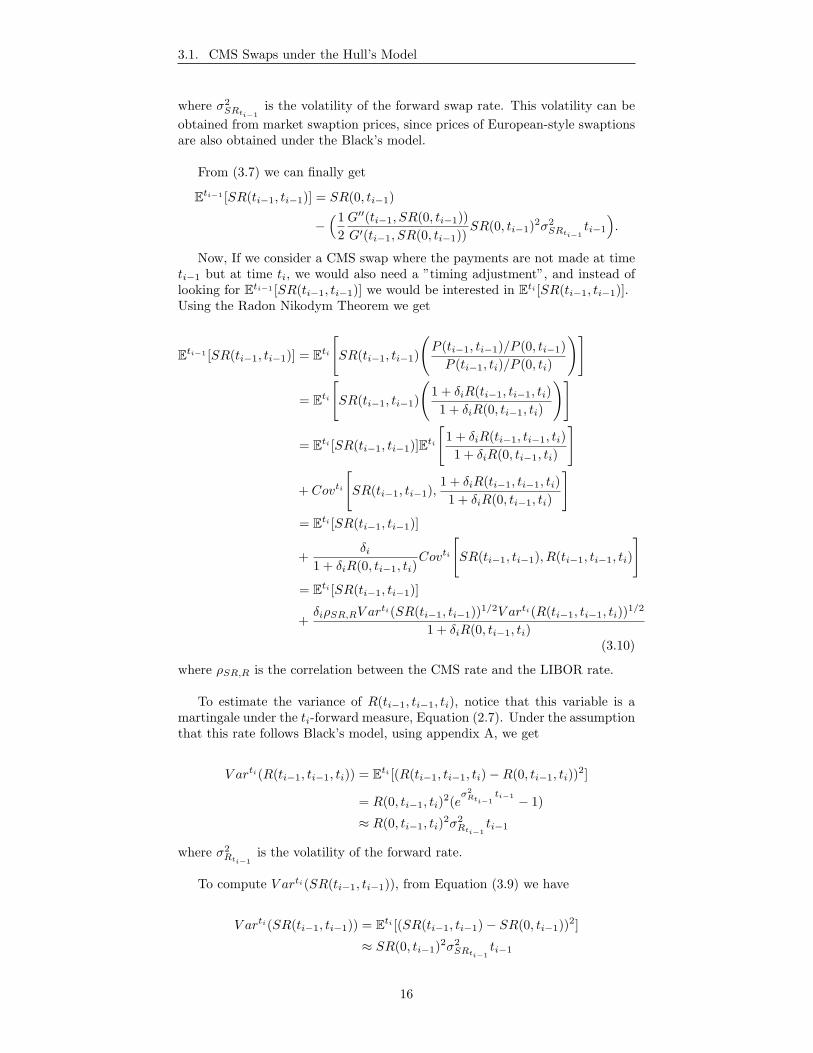
Now, If we consider a CMS swap where the payments are not made at timeti−1 but at time ti, we would also need a ”timing adjustment”, and instead oflooking for Eti−1 [SR(ti−1, ti−1)] we would be interested in Eti [SR(ti−1, ti−1)].Using the Radon Nikodym Theorem we get
Eti−1 [SR(ti−1, ti−1)] = Eti[SR(ti−1, ti−1)
(P (ti−1, ti−1)/P (0, ti−1)P (ti−1, ti)/P (0, ti)
)]
= Eti[SR(ti−1, ti−1)
(1 + δiR(ti−1, ti−1, ti)
1 + δiR(0, ti−1, ti)
)]
= Eti [SR(ti−1, ti−1)]Eti[
1 + δiR(ti−1, ti−1, ti)1 + δiR(0, ti−1, ti)
]
+ Covti
[SR(ti−1, ti−1),
1 + δiR(ti−1, ti−1, ti)1 + δiR(0, ti−1, ti)
]= Eti [SR(ti−1, ti−1)]
+δi
1 + δiR(0, ti−1, ti)Covti
[SR(ti−1, ti−1), R(ti−1, ti−1, ti)
]= Eti [SR(ti−1, ti−1)]
+δiρSR,RV ar
ti(SR(ti−1, ti−1))1/2V arti(R(ti−1, ti−1, ti))1/2
1 + δiR(0, ti−1, ti)(3.10)
where ρSR,R is the correlation between the CMS rate and the LIBOR rate.
To estimate the variance of R(ti−1, ti−1, ti), notice that this variable is amartingale under the ti-forward measure, Equation (2.7). Under the assumptionthat this rate follows Black’s model, using appendix A, we get
V arti(R(ti−1, ti−1, ti)) = Eti [(R(ti−1, ti−1, ti)−R(0, ti−1, ti))2]
= R(0, ti−1, ti)2(eσ2Rti−1
ti−1 − 1)
≈ R(0, ti−1, ti)2σ2Rti−1
ti−1
where σ2Rti−1
is the volatility of the forward rate.
To compute V arti(SR(ti−1, ti−1)), from Equation (3.9) we have
V arti(SR(ti−1, ti−1)) = Eti [(SR(ti−1, ti−1)− SR(0, ti−1))2]
≈ SR(0, ti−1)2σ2SRti−1
ti−1
16
3.2. CMS Swaps under the Linear Swap Rate Model (LSM)
where σ2SRti−1
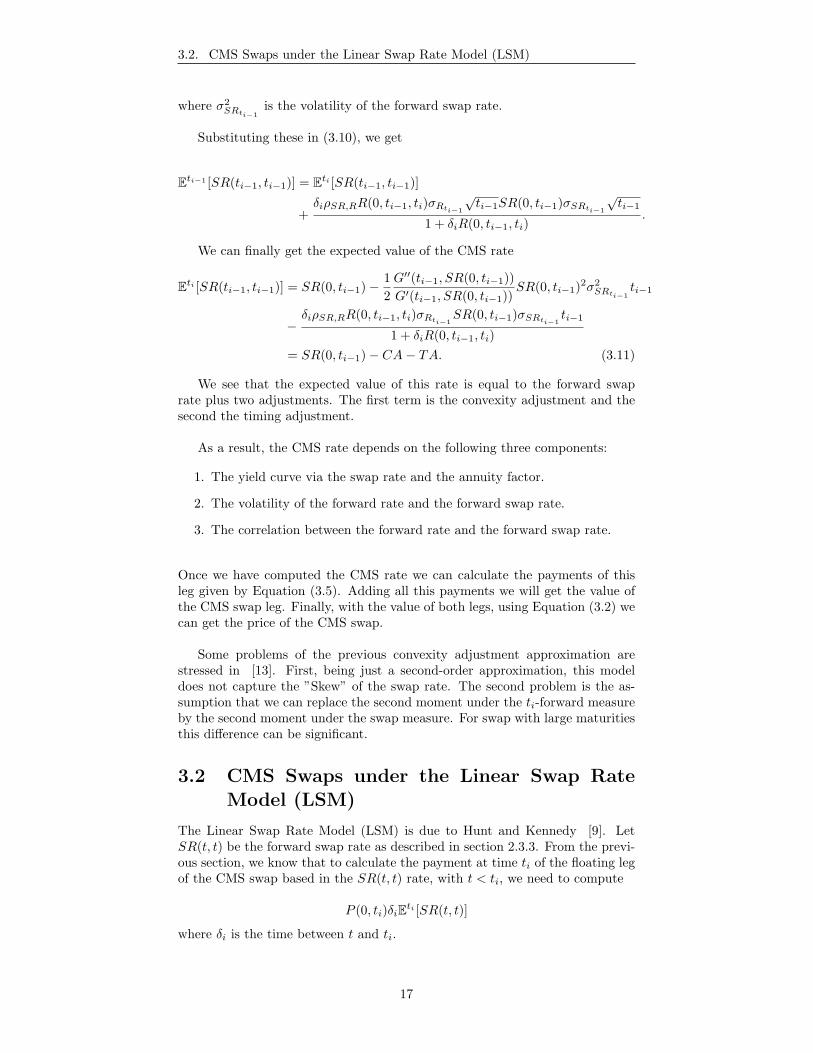
is the volatility of the forward swap rate.
Substituting these in (3.10), we get
Eti−1 [SR(ti−1, ti−1)] = Eti [SR(ti−1, ti−1)]
+δiρSR,RR(0, ti−1, ti)σRti−1
√ti−1SR(0, ti−1)σSRti−1
√ti−1
1 + δiR(0, ti−1, ti).
We can finally get the expected value of the CMS rate
We see that the expected value of this rate is equal to the forward swaprate plus two adjustments. The first term is the convexity adjustment and thesecond the timing adjustment.
As a result, the CMS rate depends on the following three components:
1. The yield curve via the swap rate and the annuity factor.
2. The volatility of the forward rate and the forward swap rate.
3. The correlation between the forward rate and the forward swap rate.
Once we have computed the CMS rate we can calculate the payments of thisleg given by Equation (3.5). Adding all this payments we will get the value ofthe CMS swap leg. Finally, with the value of both legs, using Equation (3.2) wecan get the price of the CMS swap.
Some problems of the previous convexity adjustment approximation arestressed in [13]. First, being just a second-order approximation, this modeldoes not capture the ”Skew” of the swap rate. The second problem is the as-sumption that we can replace the second moment under the ti-forward measureby the second moment under the swap measure. For swap with large maturitiesthis difference can be significant.
3.2 CMS Swaps under the Linear Swap RateModel (LSM)
The Linear Swap Rate Model (LSM) is due to Hunt and Kennedy [9]. LetSR(t, t) be the forward swap rate as described in section 2.3.3. From the previ-ous section, we know that to calculate the payment at time ti of the floating legof the CMS swap based in the SR(t, t) rate, with t < ti, we need to compute
P (0, ti)δiEti [SR(t, t)]
where δi is the time between t and ti.
17
3.2. CMS Swaps under the Linear Swap Rate Model (LSM)
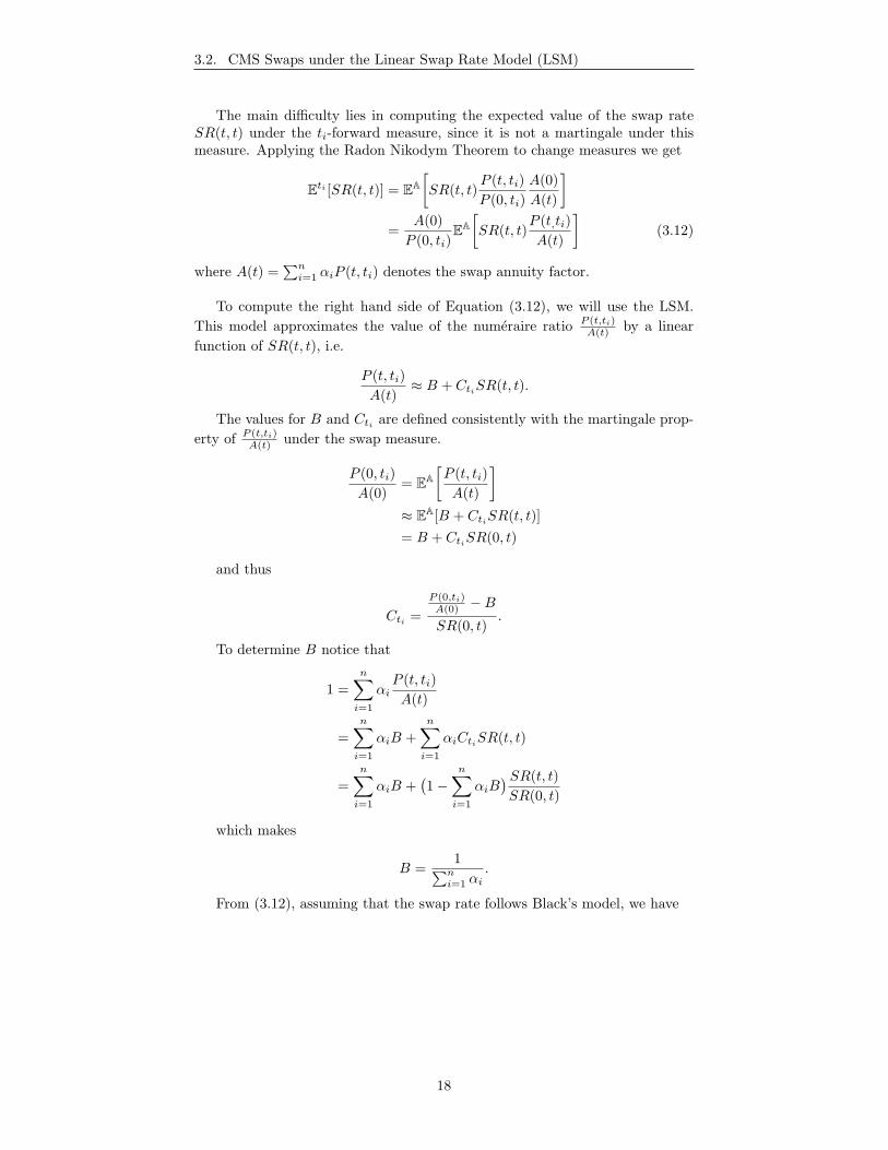
The main difficulty lies in computing the expected value of the swap rateSR(t, t) under the ti-forward measure, since it is not a martingale under thismeasure. Applying the Radon Nikodym Theorem to change measures we get
Eti [SR(t, t)] = EA[SR(t, t)
P (t, ti)P (0, ti)
A(0)A(t)
]=
A(0)P (0, ti)
EA[SR(t, t)
P (t,ti)A(t)
](3.12)
where A(t) =∑ni=1 αiP (t, ti) denotes the swap annuity factor.
To compute the right hand side of Equation (3.12), we will use the LSM.This model approximates the value of the numeraire ratio P (t,ti)
A(t) by a linearfunction of SR(t, t), i.e.
P (t, ti)A(t)
≈ B + CtiSR(t, t).
The values for B and Cti are defined consistently with the martingale prop-erty of P (t,ti)
A(t) under the swap measure.
P (0, ti)A(0)
= EA[P (t, ti)A(t)
]≈ EA[B + CtiSR(t, t)]= B + CtiSR(0, t)
and thus
Cti =P (0,ti)A(0) −BSR(0, t)
.
To determine B notice that
1 =n∑i=1
αiP (t, ti)A(t)
=n∑i=1
αiB +n∑i=1
αiCtiSR(t, t)
=n∑i=1
αiB +(1−
n∑i=1
αiB) SR(t, t)SR(0, t)
which makes
B =1∑ni=1 αi
.
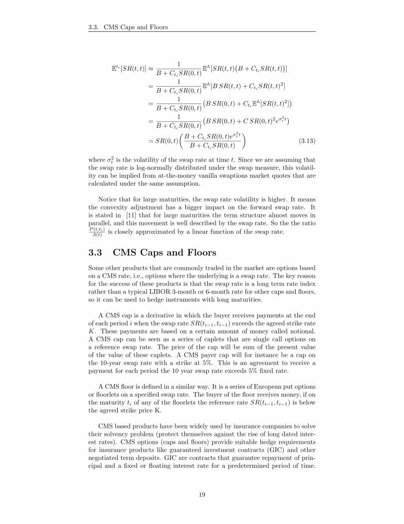
From (3.12), assuming that the swap rate follows Black’s model, we have
18
3.3. CMS Caps and Floors
Eti [SR(t, t)] ≈ 1B + CtiSR(0, t)
EA[SR(t, t)(B + CtiSR(t, t)
)]
=1
B + CtiSR(0, t)EA[B SR(t, t) + CtiSR(t, t)2]
=1
B + CtiSR(0, t)(B SR(0, t) + CtiEA[SR(t, t)2]
)=
1B + CtiSR(0, t)
(B SR(0, t) + C SR(0, t)2eσ
2t t)
= SR(0, t)(B + CtiSR(0, t)eσ
2t t
B + CtiSR(0, t)
)(3.13)
where σ2t is the volatility of the swap rate at time t. Since we are assuming that
the swap rate is log-normally distributed under the swap measure, this volatil-ity can be implied from at-the-money vanilla swaptions market quotes that arecalculated under the same assumption.
Notice that for large maturities, the swap rate volatility is higher. It meansthe convexity adjustment has a bigger impact on the forward swap rate. Itis stated in [11] that for large maturities the term structure almost moves inparallel, and this movement is well described by the swap rate. So the the ratioP (t,ti)A(t) is closely approximated by a linear function of the swap rate.
3.3 CMS Caps and Floors
Some other products that are commonly traded in the market are options basedon a CMS rate, i.e., options where the underlying is a swap rate. The key reasonfor the success of these products is that the swap rate is a long term rate indexrather than a typical LIBOR 3-month or 6-month rate for other caps and floors,so it can be used to hedge instruments with long maturities.
A CMS cap is a derivative in which the buyer receives payments at the endof each period i when the swap rate SR(ti−1, ti−1) exceeds the agreed strike rateK. These payments are based on a certain amount of money called notional.A CMS cap can be seen as a series of caplets that are single call options ona reference swap rate. The price of the cap will be sum of the present valueof the value of these caplets. A CMS payer cap will for instance be a cap onthe 10-year swap rate with a strike at 5%. This is an agreement to receive apayment for each period the 10 year swap rate exceeds 5% fixed rate.
A CMS floor is defined in a similar way. It is a series of European put optionsor floorlets on a specified swap rate. The buyer of the floor receives money, if onthe maturity ti of any of the floorlets the reference rate SR(ti−1, ti−1) is belowthe agreed strike price K.
CMS based products have been widely used by insurance companies to solvetheir solvency problem (protect themselves against the rise of long dated inter-est rates). CMS options (caps and floors) provide suitable hedge requirementsfor insurance products like guaranteed investment contracts (GIC) and othernegotiated term deposits. GIC are contracts that guarantee repayment of prin-cipal and a fixed or floating interest rate for a predetermined period of time.
19
3.3. CMS Caps and Floors
Guaranteed investment contracts are typically issued by life insurance compa-nies and often bought for retirement plans.
CMS based products provide a suitable hedge to liabilities arising from GIC.A CMS Floor for instance, provides a hedge to GIC’s when rates are falling andthe insurance company has to make guaranteed fixed interest payments. Simi-larly, CMS caps provide hedge in a rising environment.
The payoff of each CMS caplet/floorlet at time ti is given by
• Lδi max [SR(ti−1, ti−1)−K, 0]
• Lδi max [K − SR(ti−1, ti−1), 0]
where L is the principal, δi is the time between time ti and ti−1.
Practitioners focus on the computation of the forward CMS rate as they usethis adjusted rate to price simple options on CMS (cap, floor, swaption). Oncethat the CMS rate has been adjusted they use it in the Black’s model to priceoptions.
To compute the value at time zero of a caplet, according to the option pricingtheory, we need to compute the expected value of the discounted payoff underthe martingale measure. Since the payoff is made at time ti we will use theti-forward measure. Then we have
Lδi P (0, ti)Eti[
max[SR(ti−1, ti−1)−K, 0]].
From the log-normal assumption, and using appendix B, we have that thevalue of the expected payoff at time 0 is given by
Lδi P (0, ti)[Eti [SR(ti−1, ti−1)]N(d1)−KN(d2)
].
where N(x) denotes the standard normal cumulative distribution function.
We know the value of Eti [SR(ti−1, ti−1)], this is the adjusted swap rate fromprevious chapters, Equation (3.11) and Equation (3.13). This adjusted rate willbe denoted by SR(0, ti−1)′.
The values for d1 and d2 are given by
d1 =ln(SR(0,ti−1)′
K ) + σ2ti−12
σ√ti−1
d2 = d1 − σ√ti−1.
Notice that the volatility σ is multiplied by√ti−1 because the swap rate
SR(ti−1, ti−1) is observed at time ti−1. The discount factor P (0, ti) reflects thefact that the payoff is at time ti.
The value of the corresponding floorlet is given by
Lδi P (0, ti)[KN(−d2)− Eti [SR(ti−1, ti−1)]N(−d1)
].
It has been emphasized in [7] that the main problem with the Black’s modelis that it does not consider the smile or skew observed in the market volatility.And some recommendations to diminish this problem are made there. For a
20
3.3. CMS Caps and Floors
CMS swap the volatility of at-the-money swaptions should be used. Out-of-the-money caplets and floorlets can be priced using the volatility for the strike K,and finally for in-the-money caplets or floorlets the call-put parity should beused, i.e. the price of an in-the-money caplet will be the price of a CMS swapplus the price of an out-of-the-money floorlet.
21
Chapter 4
Average CMS options
Average (Asian) options are path-dependant securities which payoff depends onthe average of the underlying asset price over certain time interval. Stock prices,stock indices, commodities, exchange rates, and interest rates are example ofunderlying assets. Since no general analytical solution for the price of the Asianoption is known, a variety of techniques have been developed to analyse theprice of these financial instruments.
Asian options have a lower volatility, that makes them cheaper relative totheir European counterparts. They were introduced partly to avoid a commonproblem for European options, where the speculators could drive up the gainsfrom the option by manipulating the price of the underlying asset near to thematurity. The name ”Asian option” probably originates from the Tokyo officeof bankers Trust, where it was first offered.
In this chapter we present a method to approximate the value of averageCMS options (caps and floors). As explained in section 3.3, a cap or floor canbe seen as a series of caplets or floorlets respectively, that are single options ona reference rate. For the case of an Asian CMS cap, the price of every singlecaplet will be calculated, to later add them up and have the price of the cap.
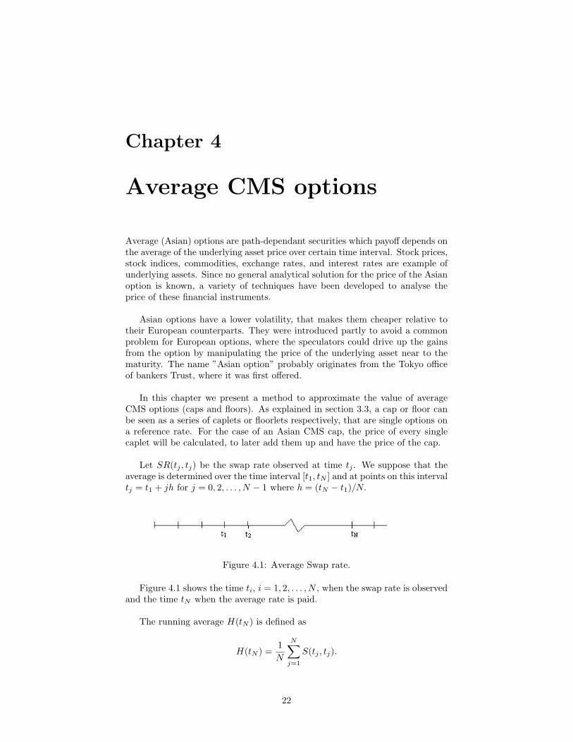
Let SR(tj , tj) be the swap rate observed at time tj . We suppose that theaverage is determined over the time interval [t1, tN ] and at points on this intervaltj = t1 + jh for j = 0, 2, . . . , N − 1 where h = (tN − t1)/N.
Figure 4.1: Average Swap rate.
Figure 4.1 shows the time ti, i = 1, 2, . . . , N , when the swap rate is observedand the time tN when the average rate is paid.
The running average H(tN ) is defined as
H(tN ) =1N
N∑j=1
S(tj , tj).
22
4.1. Levy Log-normal Approximation
The average CMS option is characterized by the payoff function at time tNgiven by
LδtN max[H(tN )−K, 0
](4.1)
for a caplet option, and
LδtN max[K −H(tN ), 0
](4.2)
for a floorlet option. In both cases L is the notional, δtN is the time betweeneach caplet/floorlet payment, and K is the strike price of the option.
4.1 Levy Log-normal Approximation
To price the average CMS option we will need to compute the distribution ofthe arithmetic average. It is well known that no analytical solution exists forthe price of European calls or puts written on the arithmetic average when theunderlying index follows a log-normal process described in Section 3.1, equation(3.1).
Hence, the pricing of such options becomes an interesting field in finance.We will use an approximation by Levy [10], that consists in approximate theaverage H(tN ) with a log-normal distribution. This approach relies on the factthat all the moments of the arithmetic average can be easily calculated eventhough the distribution of the average is unknown.
Based on the risk neutral pricing method, the value C at time 0 of a capletwith payoff given by equation (4.1) is
C = P (0, tN ) δtNEtN[
max[H(tN )−K, 0]]
where EtN denotes the expectation under the tN -forward measure.
Under the log-normal distribution assumption, the value of the last expec-tation will be a Black-Scholes style formula. Denoting by f(x) the log-normalprobability density function, we have
EtN[Max [H(tN )−K, 0]
]=∫ ∞K
xf(x) dx−K∫ ∞K
f(x) dx.
To solve the first integral∫ ∞K
xf(x) dx =∫ ∞K
x1
λx√
2πexp
(− (lnx− ν)2
2λ2
)dx
we will use a change of variable
y =ν + λ2 − lnx
λdy = − 1
λxdx.
It follows∫ ∞K
xf(x) dx =∫ ∞ν+λ2−lnK
λ
− exp(ν + λ2 − λy)1√2π
exp(− 1
2(y − λ)2
)dy
= exp(ν +12λ2)
∫ ν+λ2−lnKλ
∞
1√2π
exp(−12y2) dy
= exp(ν +12λ2)N
(ν + λ2 − lnKλ
)(4.3)
23
4.1. Levy Log-normal Approximation
where N(x) denotes the standard normal cumulative distribution.
To compute the second integral we go along the same lines, using the changeof variable
z =ν − lnx
λdz = − 1
λxdx
we get ∫ ∞K
xf(x) dx = N(ν − lnK
λ
). (4.4)
Using (4.3) and (4.4) the price of a CMS caplet option is
C = P (0, tN ) δTN(
exp(ν +12λ2)N(d1)−KN(d2)
)(4.5)
where
d1 =ν + λ2 − lnK
λ(4.6)
d2 = d1 − λ. (4.7)
The parameters ν and λ can be estimated from the following expression fora log-normal distribution
E[H(tN )s] = esν+ 12 s
2λ2. (4.8)
Estimating the first and second moments, we get
ν = 2 ln E[H(tN )]− 12
ln E[H(tN )2]
λ2 = ln E[H(tN )2]− 2 ln E[H(tN )].
We still have to compute the moments of the average variable H(tN ) underthe tN forward measure. The first moment is given by
EtN [H(tN )] = EtN [1N
N∑j=1
S(tj , tj)]
=1N
N∑j=1
EtN [S(tj , tj)]
=1N
N∑j=1
S(0, tj)′
where S(0, tj)′ denotes the convexity adjusted rate that we have extensivelyworked out in Chapter 3, equations (3.11) and (3.13). We need this convex-ity adjusted rate because for the valuation of the caplet we work under thetN -forward measure rather than the martingale measure for the swap rate. An-other difference in these payments is that they are not made one period afterthe rate is observed, but at the end of the average period. So for each swap rateobserved at time ti and considered in the average payment made at time tN ,the timing adjustment will be made for these associated two forward measures.
24
4.1. Levy Log-normal Approximation
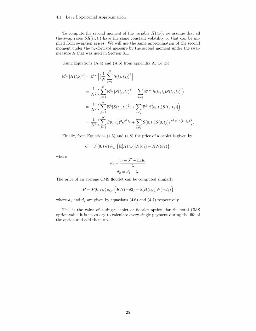
To compute the second moment of the variable H(tN ), we assume that allthe swap rates SR(ti, ti) have the same constant volatility σ, that can be im-plied from swaption prices. We will use the same approximation of the secondmoment under the tN -forward measure by the second moment under the swapmeasure A that was used in Section 3.1.
Using Equations (A.4) and (A.6) from appendix A, we get
EtN [H(tN )2] = EtN[( 1N
N∑j=1
S(tj , tj))2]
=1N2
( N∑j=1
EtN [S(tj , tj)2] +∑i6=j
EtN [S(ti, ti)S(tj , tj)])
≈ 1N2
( N∑j=1
EA[S(tj , tj)2] +∑i 6=j
EA[S(ti, ti)S(tj , tj)])
=1N2
( N∑j=1
S(0, tj)2eσ2tj +
∑i 6=j
S(0, ti)S(0, tj)eσ2 minti,tj
).
Finally, from Equations (4.5) and (4.8) the price of a caplet is given by
C = P (0, tN ) δtN(E[H(tN )]N(d1)−KN(d2)
).
where
d1 =ν + λ2 − lnK
λ
d2 = d1 − λ.
The price of an average CMS floorlet can be computed similarly
P = P (0, tN ) δtN(KN(−d2)− E[H(tN )]N(−d1)
)where d1 and d2 are given by equations (4.6) and (4.7) respectively.
This is the value of a single caplet or floorlet option, for the total CMSoption value it is necessary to calculate every single payment during the life ofthe option and add them up.
25
Chapter 5
Pricing CMS Derivativeswith Monte CarloSimulation
Derivatives valuation involves the computation of expected values of complexfunctional of random paths. The Monte Carlo method can be applied to com-pute approximated values for these quantities. This method plays an importantrole in the valuation of some interest rate derivatives, that usually require thesimulation of the entire yield curve. It simulates the component that includesuncertainty. We will use a Monte Carlo approximation to implement a shortrate model.
The short rate, r, is the rate that applies to an infinitesimally short periodof time. Derivatives prices depend on the process followed by r in a risk neutralworld. The most common short rate models are single-factor Markovian models,where there is only one source of uncertainty and the evolution of the short ratedoes not depend on previous interest rate movements. Some examples of thesemodels are the Vasicek, Ho-Lee or Hull-White model. These models are widelyused since they are easily implemented and under them some derivatives havea price expressed in a closed formula.
These models are described by a Stochastic Differential Equation (SDE),that under the risk neutral measure Q has the form
drt = µ(rt)dt+ σ(rt)dWt (5.1)
where µ is the drift function, σ is the diffusion function and W is a Q-Brownianmotion. The short rate models differ from each other in how the functions µand σ are defined.
5.1 Hull-White Model
The Hull-White model (1994) is one of the no-arbitrage models that is designedto be consistent with the actual term structure of interest rate. In this model,also called extended Vasicek model, the function µ(r) is defined as
µ(r) = θ − ar
26
5.1. Hull-White Model
where a is a constant that represents the mean reversion parameter and θ is afunction determined uniquely by the term structure.
The SDE that defines the Hull-White model is then given by
drt = [θt − art]dt+ σdWt (5.2)
the constants a and σ will be determined by a calibration process. In practice,the Hull-White model is calibrated by choosing the mean reversion rate andvolatility in such a way so that they are consistent with option prices observedin the market.
The model implies that the short-term rate is normally distributed and sub-ject to mean reversion. The mean reversion parameter a ensures consistencywith the empirical observation that long rates are less volatile than short rates.
Lemma 5.1.1. The process rt is normally distributed with mean
E[rt] = e−atr0 +∫ t
0
e−a(t−u)θudu (5.3)
and variance
V ar[rt] =σ2
2a(1− e−2at). (5.4)
Proof. Let Xt = eatrt, by Ito’s lemma we get
dXt =∂X
∂rtdrt +
∂X
∂tdt+
12∂2X
∂r2t
[dXt]2
= eatdrt + eatart dt.
Substituting the dynamics of drt, Equation (5.2), and expressing dXt inintegral form, we get
Xt = X0 +∫ t
0
eau(θu − aru)du+∫ t
0
eauσdWu +∫ t
0
eauarudu
= X0 +∫ t
0
eauθudu+∫ t
0
eauσdWu.
Then
rt = e−atXt
= e−atr0 +∫ t
0
e−a(t−u)θudu+∫ t
0
e−a(t−u)σdWu. (5.5)
We can now compute the moments of this random variable. First, noticethat
E[∫ t
0
e−a(t−u)σdWu] = 0
then we have
E[rt] = e−atr0 +∫ t
0
e−a(t−u)θudu
27
5.1. Hull-White Model
and the variance is given by
V ar[rt] = E[rt − E[rt]
]2= E
[ ∫ t
0
e−a(t−u)σdWu
]2
= E[σ2
∫ t
0
e−2a(t−u)du
]=σ2
2a(1− e−2at).
5.1.1 Bond and Option pricing
We denote by P (t, T ) the price at time t of a zero coupon bond maturing attime T . It’s value is given by
P (t, T ) = EQ[e−∫ Ttrsds|Ft].
where Q denotes the risk neutral measure. In order to compute this expectationwe need to know the distribution of
∫ Ttrsds. Define
B(t, T ) =1− e−a(T−t)
a. (5.6)
From Equation (5.5), integrating rs from t to T , and interchanging integrals weget∫ T
t
rsds =∫ T
t
e−asr0 ds+∫ T
t
∫ s
0
e−a(s−u)θu du ds+∫ T
t
∫ s
0
e−a(s−u)σ dWu ds
=∫ T
t
e−asr0 ds+∫ t
0
∫ T
t
e−a(s−u)θu ds du+∫ T
t
∫ T
u
e−a(s−u)θu ds du
+∫ t
0
∫ T
t
e−a(s−u)σ ds dWu +∫ T
t
∫ T
u
e−a(s−u)σ ds dWu.
Using (5.6) we rewrite this as
∫ T
t
rsds = r0e−atB(t, T ) + e−atB(t, T )
∫ t
0
eauθu du+∫ T
t
B(u, T )θu du
+ e−atσB(t, T )∫ t
0
eau dWu + σ
∫ T
t
B(u, T ) dWu
= rtB(t, T ) +∫ T
t
B(u, T )θu du+ σ
∫ T
t
B(u, T ) dWu.
It follows that∫ Ttrsds is conditionally normally distributed with
E[∫ T
t
rsds|Ft] = rtB(t, T ) +∫ T
t
B(u, T )θudu
and variance
V ar[∫ T
t
rudu|Ft] = σ2
∫ T
t
B(u, T )2du.
28
5.1. Hull-White Model
Thus, the bond price can be calculated as the expected value of a log-normaldistributed variable.
P (t, T ) = EQ[e−∫ Ttrsds|Ft]
= e−rtB(t,T )−∫ TtB(u,T )θudu+ 1
2σ2 ∫ TtB(u,T )2du
= eA(t,T )−B(t,T )rt
where
A(t, T ) =∫ T
t
(12σ2B(u, T )2 −B(u, T )θu
)du. (5.7)
We have not given an explicit formula for the function θT , but we mentionedthat it can be calculated from the initial term structure of the instantaneousforward rate. Denoting the theoretical instantaneous forward rate observed attime zero with maturity T by f(0, T ), we have that its value is given by
f(0, T ) = −∂ lnP (0, T )∂T
= −∂(A(0, T )−B(0, T )r0)∂T
.
From Equation (5.7) we have
∂A(0, T )∂T
=12σ2B(T, T )2 + σ2
∫ T
0
B(u, T )∂B(u, T )∂T
du
−B(T, T )θT −∫ T
0
∂B(u, T )∂T
θu du
and from Equation (5.6) we get
∂B(t, T )∂T
= e−a(T−t).
Putting this together we get
f(0, T ) = −∂A(0, T )∂T
+∂B(0, T )∂T
r0
=∫ T
0
e−a(T−u)θu du+σ2
a2
[12
(1− e−2aT )− (1− e−aT )]
+ e−aT r0.
(5.8)
Taking the derivative with respect to T to get the value of θT , we have
∂f(0, T )∂T
= θT − a∫ T
t
e−a(T−u)θu du+σ2
a
(e−2aT − e−aT
)− ae−aT r0.
Using Equation (5.8) last equation can be written as
∂f(0, T )∂T
= θT − af(0, T ) +σ2
a
[12
(1− e−2aT )− (1− e−aT )]
+ ae−aT r0 +σ2
a
(e−2aT − e−aT
)− ae−aT r0
= θT − af(0, T )− σ2
2a(1− e−2aT
).
29
5.1. Hull-White Model
If we denote by fM (0, T ) the market instantaneous forward rate, we wouldlike to match the theoretical rate f(0, T ) with the observed rate, which means
θT =∂fM (0, T )
∂T+ afM (0, T ) +
σ2
2a(1− e−2aT ). (5.9)
This procedure is called fitting the model to the term structure of interest rate.
We can finally get the bond price substituting (5.9) into Equation (5.7).This yields
P (t, T ) =PM (0, T )PM (0, t)
exp(B(t, T )fM (0, t)− σ2
4a(1− e−2at)B(t, T )2 −B(t, T )rt
),
(5.10)where PM (0, T ) denotes the market bond price seeing at time zero with matu-rity T .
5.1.2 Simulation of the short interest rate
A more convenient representation of rt, uses a deterministic function αt thatreflects the term structure at time 0, and a random process xt, that is indepen-dent of market data.
From Equation (5.5) we have that the short rate rt can be expressed as
rt = e−atr0 +∫ t
0
e−a(t−u)θudu+∫ t
0
e−a(t−u)σdWu
= αt + xt (5.11)
where
αt = e−atr0 +∫ t
0
e−a(t−u)θudu
and
xt =∫ t
0
e−a(t−u)σ dWu. (5.12)
Substituting Equation (5.9) into the expression for αt, we get
αt = e−atr0 +∫ t
0
e−a(t−u)[∂fM (0, u)
∂u+ afM (0, u) +
σ2
2a(1− e−2au)
]du
= e−atr0 + e−at[ ∫ t
0
eau∂fM (0, u)
∂udu+
∫ t
0
eauafM (0, u)du
+∫ t
0
eauσ2
2a(1− e−2au)du
]= fM (0, t) +
σ2
2a2(1− e−at)2.
To simulate the evolution of rt, we will use an Euler scheme, the simplestand most common discretization scheme. We have that for a small time step∆, Equation (5.1) can be approximated by
The increments W∆(t+1) −W∆t are independent normally distributed variableswith mean zero and variance ∆.
For the Hull-White model, we will apply this approximation to the processxt defined by Equation (5.12). Then we have
ea∆(t+1)x∆(t+1) − ea∆tx∆t = σ
∫ ∆(t+1)
∆t
eaudWu.
Notice that these variables are also normally distributed with mean zero andvariance
σ2
∫ ∆(t+1)
∆t
e2audu = σ2e2a∆t e2a∆ − 1
2a.
Hence
ea∆(t+1)x∆(t+1) − ea∆tx∆t ∼ ea∆t
√12σ2e2a∆ − 1
2aZk, (5.14)
where Zk is a standard Gaussian random variable generated in the kth iteration.
We can finally write
x∆(t+1) − ea∆tx∆t ∼√
12σ2B(0, 2∆)Zk.
Once we have the short rate term structure rt = αt+xt, we are able to computethe bond prices P (t, T ), using formula (5.10), required to get the value of theswap rate SR(ti, ti) at time ti. This swap rate represents the pay off of theCMS leg. From Chapter 2, formula (2.12), we have
SR(ti, ti) =1− P (ti, ti + sn)∑nj=1 αjP (ti, ti + sj)
.
The discount factors P (0, T ) = EQ[e−∫ T0 rsds] will be calculated using an
approximation for the integral e−∫ T0 rsds ≈ e−∆
∑k rk .
5.1.3 Model Calibration
A term structure model has to be calibrated to the market before it can be usedfor valuation purposes. After fitting the term structure with the parameter θ,there are still two constants to be determined, a and σ. The procedure of choos-ing the constants a and σ that match market prices for certain instruments withthe prices we get with the model is called calibration.
To calibrate the model to market prices we need to find the best fit for aand σ simultaneously. In this case we will use Euro-Caplets derivatives as in-struments to calibrate the model, since they are quite liquid in the market andsince we have an analytical formula under the Hull-White model to price them,see Equation (5.16).
So, if we have M European caplet prices, we should minimize the function
M∑i=1
(model(a, σ)i −marketimarketi
)2
(5.15)
31
5.1. Hull-White Model
where model(a, σ)i and marketi stand for model and market prices respectively.
We will use the Euro-caplets volatility quotes from the market to calculatethe market prices. According to the Black’s model, mentioned in section 3.3,the volatilities uniquely determined the caplet prices. The model prices will becomputed using the analytical formulas under the Hull-White model providedin next subsection.
Finally, to minimize the previous function we will use a Levenberg-Marquardtalgorithm, that is a popular alternative to the Gauss-Newton method of findingthe minimum of a function that is a sum of squares of nonlinear functions.
Caplet Prices under the Hull-White Model
To price European options with maturity at time T under the Hull-White model,we need to compute the expected value of the payoff under the T -forward mea-sure. We will need to express the dynamics of the short rate rt, given by equation(5.11), under this measure. An application of Girsanov’s Theorem is used tochange the dynamics of the process xt, used in the decomposition of rt = αt+xt,from the Q risk-neutral measure to the T -forward measure, see Brigo [4]. Thenwe have
dx(t) =[−B(t, T )σ2 − ax(t)
]dt+ σdWT (t)
dWT (t) = dW (t) + σB(t, T ) dt
where B(t, T ) is given by Equation (5.6), and WT is a Brownian motion underthe T -forward measure.
Then for s ≤ t ≤ T
xt = xse−a(t−s) −MT (s, t) + σ
∫ t
s
e−a(t−u)dWT (u)
with
MT (s, t) =σ2
a2
[1− e−a(t−s)]− σ2
2a2
[e−a(T−t) − e−a(T+t−2s)
].
The short rate rt conditional on Fs and under the T -forward measure, isnormally distributed with mean and variance given by
E[rt|Fs] = xse−a(t−s) −MT (s, t) + α(t)
V ar[rt|Fs] =σ2
2a(1− e−2a(t−s)).
Under this distribution, we can calculate the price at time t of a Europeancaplet on a rate L(T, S), that can be a Euribor rate for the period [T, S]. Thisrate is reset at time T and paid at time S. If the cap rate is equal to K and thenotional value is X then its price is given by 1
1The following formulas can be derived through the same methodology given in AppendixB.
32
5.1. Hull-White Model
where
h1 =1σplnP (t, S)(1 +Kτ)
P (t, T )+σ2p
2
h2 = h1 − σpand
σp = σ
√1− e−2a(T−t)
2aB(T, S).
33
Chapter 6
Example of CMSDerivatives
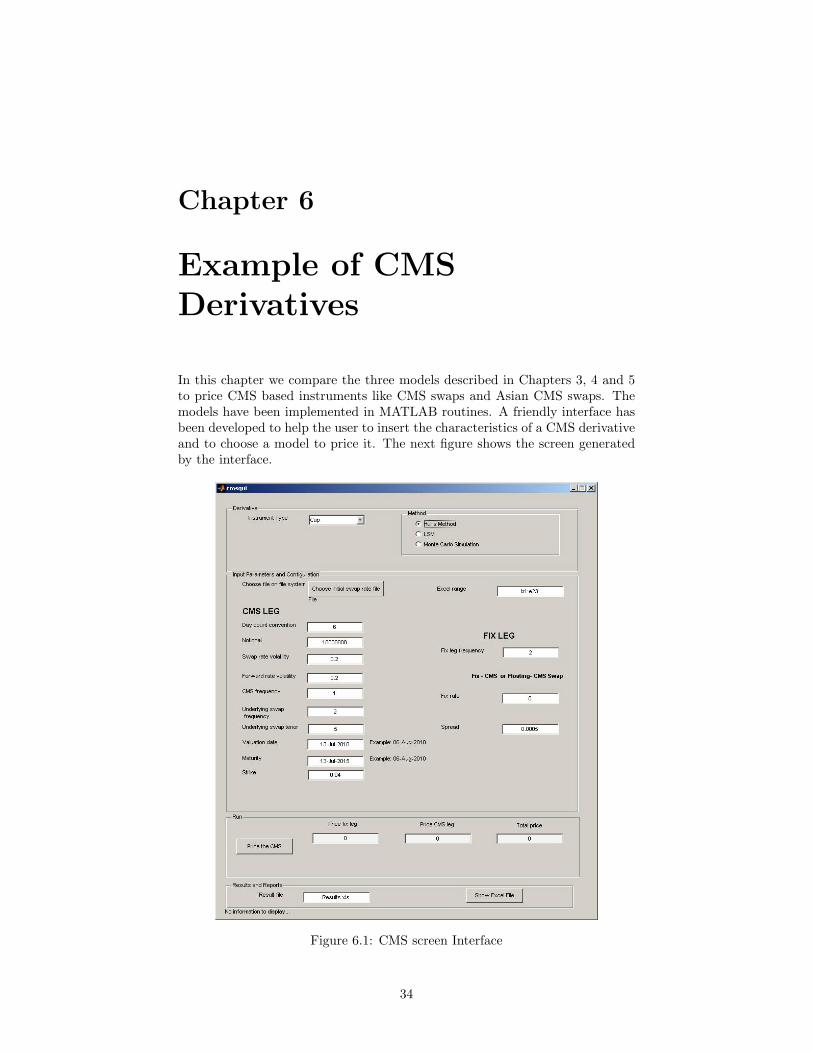
In this chapter we compare the three models described in Chapters 3, 4 and 5to price CMS based instruments like CMS swaps and Asian CMS swaps. Themodels have been implemented in MATLAB routines. A friendly interface hasbeen developed to help the user to insert the characteristics of a CMS derivativeand to choose a model to price it. The next figure shows the screen generatedby the interface.
Figure 6.1: CMS screen Interface
34
6.1. Example 1. CMS Swap
Once the screen has been filled, the instrument can be priced and an Excelfile with the results is generated. In the next two examples, we will see thisExcel file.
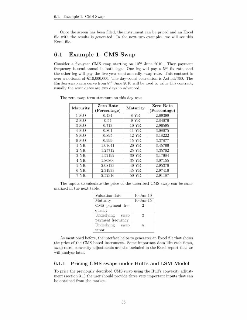
6.1 Example 1. CMS Swap
Consider a five-year CMS swap starting on 10th June 2010. They paymentfrequency is semi-annual in both legs. One leg will pay a 5% fix rate, andthe other leg will pay the five-year semi-annually swap rate. This contract isover a notional of ¤10,000,000. The day-count convention is Actual/360. TheEuribor-swap zero curve from 8th June 2010 will be used to value this contract;usually the reset dates are two days in advanced.
The zero swap term structure on this day was:
MaturityZero Rate
MaturityZero Rate
(Percentage) (Percentage)1 MO 0.434 8 YR 2.693992 MO 0.54 9 YR 2.840763 MO 0.713 10 YR 2.965954 MO 0.801 11 YR 3.080755 MO 0.895 12 YR 3.182226 MO 0.999 15 YR 3.378771 YR 1.07641 20 YR 3.457662 YR 1.25712 25 YR 3.357023 YR 1.52192 30 YR 3.176844 YR 1.80806 35 YR 3.071555 YR 2.08133 40 YR 2.953766 YR 2.31933 45 YR 2.974167 YR 2.52316 50 YR 2.91187
The inputs to calculate the price of the described CMS swap can be sum-marized in the next table.
Valuation date 10-Jun-10Maturity 10-Jun-15CMS payment fre-quency
2
Underlying swappayment frequency
2
Underlying swaptenor
5
As mentioned before, the interface helps to generates an Excel file that showsthe price of the CMS based instrument. Some important data like cash flows,swap rates, convexity adjustments are also included in the Excel report that wewill analyse later.
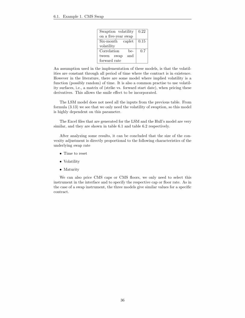
6.1.1 Pricing CMS swaps under Hull’s and LSM Model
To price the previously described CMS swap using the Hull’s convexity adjust-ment (section 3.1) the user should provide three very important inputs that canbe obtained from the market.
35
6.1. Example 1. CMS Swap
Swaption volatilityon a five-year swap
0.22
Six-month capletvolatility
0.15
Correlation be-tween swap andforward rate
0.7
An assumption used in the implementation of these models, is that the volatil-ities are constant through all period of time where the contract is in existence.However in the literature, there are some model where implied volatility is afunction (possibly random) of time. It is also a common practise to use volatil-ity surfaces, i.e., a matrix of (strike vs. forward start date), when pricing thesederivatives. This allows the smile effect to be incorporated.
The LSM model does not need all the inputs from the previous table. Fromformula (3.13) we see that we only need the volatility of swaption, so this modelis highly dependent on this parameter.
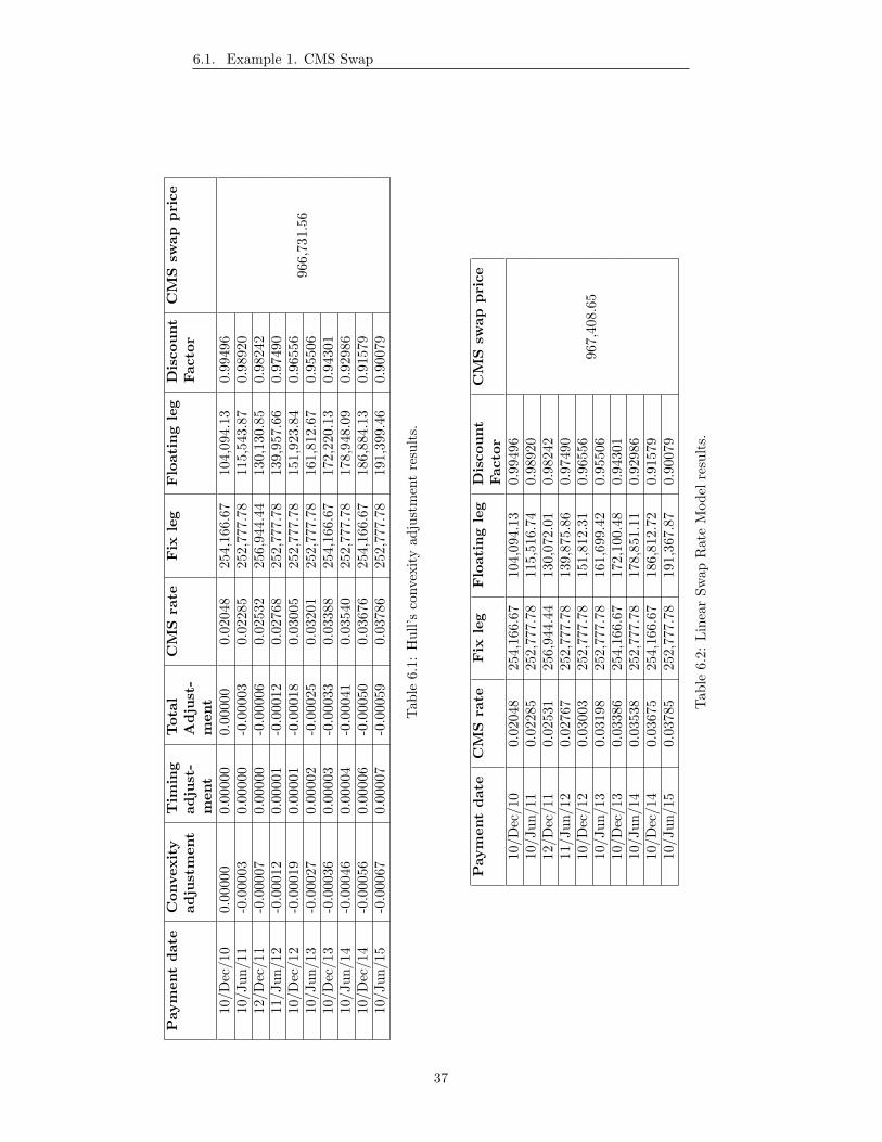
The Excel files that are generated for the LSM and the Hull’s model are verysimilar, and they are shown in table 6.1 and table 6.2 respectively.
After analyzing some results, it can be concluded that the size of the con-vexity adjustment is directly proportional to the following characteristics of theunderlying swap rate
• Time to reset
• Volatility
• Maturity
We can also price CMS caps or CMS floors, we only need to select thisinstrument in the interface and to specify the respective cap or floor rate. As inthe case of a swap instrument, the three models give similar values for a specificcontract.
36
6.1. Example 1. CMS Swap
Pay
men
td
ate
Con
vexit
yad
just
men
tT
imin
gad
just
-m
ent
Tot
alA
dju
st-
men
t
CM
Sra
teF
ixle
gF
loat
ing
leg
Dis
cou
nt
Fac
tor
CM
Ssw
app
rice
10/D
ec/1
00.
0000
00.
0000
00.
0000
00.
0204
825
4,16
6.67
104,
094.
130.
9949
6
966,
731.
56
10/J
un/1
1-0
.000
030.
0000
0-0
.000
030.
0228
525
2,77
7.78
115,
543.
870.
9892
012
/Dec
/11
-0.0
0007
0.00
000
-0.0
0006
0.02
532
256,
944.
4413
0,13
0.85
0.98
242
11/J
un/1
2-0
.000
120.
0000
1-0
.000
120.
0276
825
2,77
7.78
139,
957.
660.
9749
010
/Dec
/12
-0.0
0019
0.00
001
-0.0
0018
0.03
005
252,
777.
7815
1,92
3.84
0.96
556
10/J
un/1
3-0
.000
270.
0000
2-0
.000
250.
0320
125
2,77
7.78
161,
812.
670.
9550
610
/Dec
/13
-0.0
0036
0.00
003
-0.0
0033
0.03
388
254,
166.
6717
2,22
0.13
0.94
301
10/J
un/1
4-0
.000
460.
0000
4-0
.000
410.
0354
025
2,77
7.78
178,
948.
090.
9298
610
/Dec
/14
-0.0
0056
0.00
006
-0.0
0050
0.03
676
254,
166.
6718
6,88
4.13
0.91
579
10/J
un/1
5-0
.000
670.
0000
7-0
.000
590.
0378
625
2,77
7.78
191,
399.
460.
9007
9
Tab
le6.
1:H
ull’s
conv
exit
yad
just
men
tre
sult
s.
Pay
men
td
ate
CM
Sra
teF
ixle
gF
loat
ing
leg
Dis
cou
nt
Fac
tor
CM
Ssw
app
rice
10/D
ec/1
00.
0204
825
4,16
6.67
104,
094.
130.
9949
6
967,
408.
65
10/J
un/1
10.
0228
525
2,77
7.78
115,
516.
740.
9892
012
/Dec
/11
0.02
531
256,
944.
4413
0,07
2.01
0.98
242
11/J
un/1
20.
0276
725
2,77
7.78
139,
875.
860.
9749
010
/Dec
/12
0.03
003
252,
777.
7815
1,81
2.31
0.96
556
10/J
un/1
30.
0319
825
2,77
7.78
161,
699.
420.
9550
610
/Dec
/13
0.03
386
254,
166.
6717
2,10
0.48
0.94
301
10/J
un/1
40.
0353
825
2,77
7.78
178,
851.
110.
9298
610
/Dec
/14
0.03
675
254,
166.
6718
6,81
2.72
0.91
579
10/J
un/1
50.
0378
525
2,77
7.78
191,
367.
870.
9007
9
Tab
le6.
2:L
inea
rSw
apR
ate
Mod
elre
sult
s.
37
6.1. Example 1. CMS Swap
6.1.2 Pricing CMS swaps using Monte Carlo simulation
A Monte Carlo simulation was also implemented in a MATLAB routine. Theinputs are quite similar, but for this model the swap rate volatility, forwardrate volatility and the correlation are not required. As explained in Chapter5, to generate the short rate rt, the process xt of Equation (5.14) needs to besimulated.
The main difficulty for this simulation is to estimate the constants a and σthat are required for the Hull-White model. Unlike the other parameters, a andσ are not directly provided by the market. The MATLAB code has an opti-mization routine, that calculates these two parameters. To calibrate the modelwe need to provide market data from plain vanilla caplets. These data includecaplets maturities, implied volatilities and strikes that will be used to calculatecaplet prices using the Black’s model (1976)1.
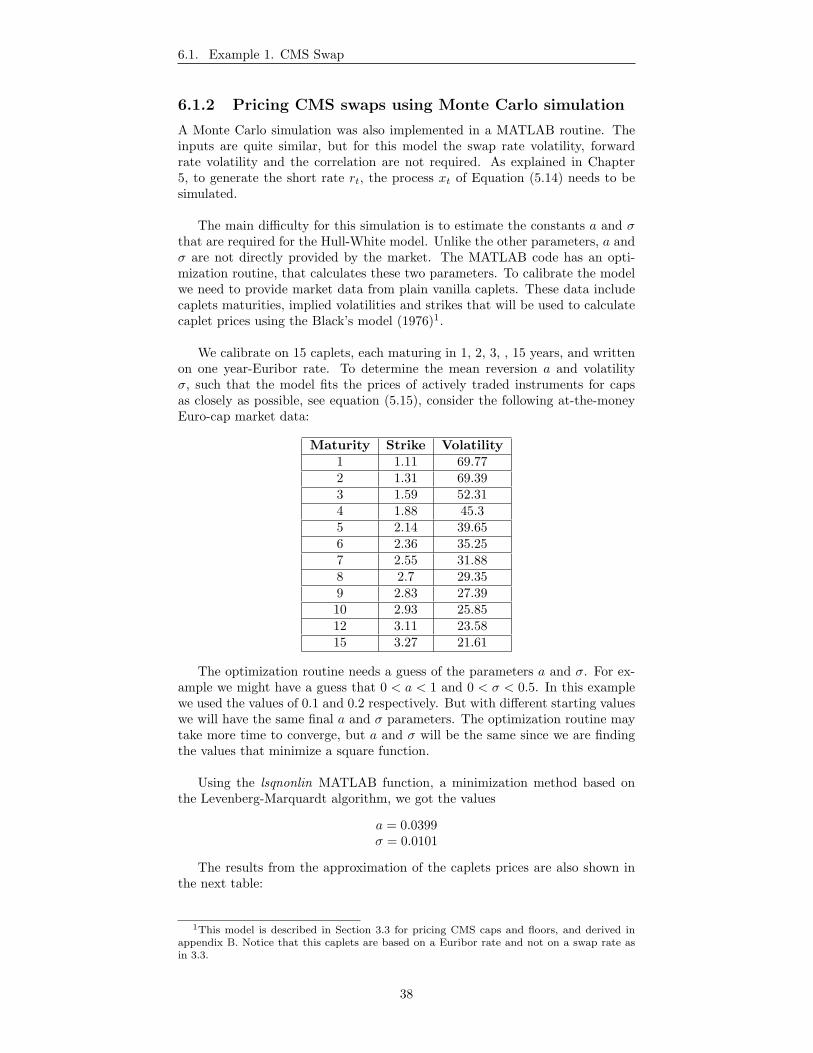
We calibrate on 15 caplets, each maturing in 1, 2, 3, , 15 years, and writtenon one year-Euribor rate. To determine the mean reversion a and volatilityσ, such that the model fits the prices of actively traded instruments for capsas closely as possible, see equation (5.15), consider the following at-the-moneyEuro-cap market data:
The optimization routine needs a guess of the parameters a and σ. For ex-ample we might have a guess that 0 < a < 1 and 0 < σ < 0.5. In this examplewe used the values of 0.1 and 0.2 respectively. But with different starting valueswe will have the same final a and σ parameters. The optimization routine maytake more time to converge, but a and σ will be the same since we are findingthe values that minimize a square function.
Using the lsqnonlin MATLAB function, a minimization method based onthe Levenberg-Marquardt algorithm, we got the values
a = 0.0399σ = 0.0101
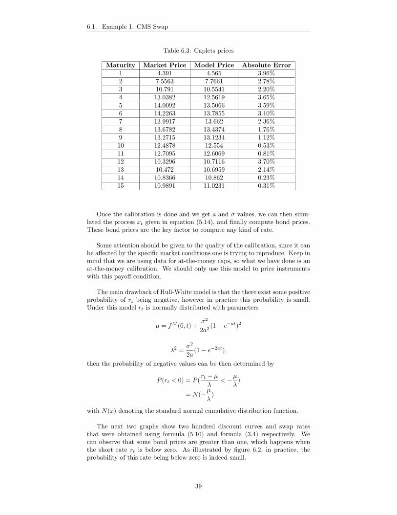
The results from the approximation of the caplets prices are also shown inthe next table:
1This model is described in Section 3.3 for pricing CMS caps and floors, and derived inappendix B. Notice that this caplets are based on a Euribor rate and not on a swap rate asin 3.3.
Once the calibration is done and we get a and σ values, we can then simu-lated the process xt given in equation (5.14), and finally compute bond prices.These bond prices are the key factor to compute any kind of rate.
Some attention should be given to the quality of the calibration, since it canbe affected by the specific market conditions one is trying to reproduce. Keep inmind that we are using data for at-the-money caps, so what we have done is anat-the-money calibration. We should only use this model to price instrumentswith this payoff condition.
The main drawback of Hull-White model is that the there exist some positiveprobability of rt being negative, however in practice this probability is small.Under this model rt is normally distributed with parameters
µ = fM (0, t) +σ2
2a2(1− e−at)2
λ2 =σ2
2a(1− e−2at),
then the probability of negative values can be then determined by
P (rt < 0) = P (rt − µλ
< −µλ
)
= N(−µλ
)
with N(x) denoting the standard normal cumulative distribution function.
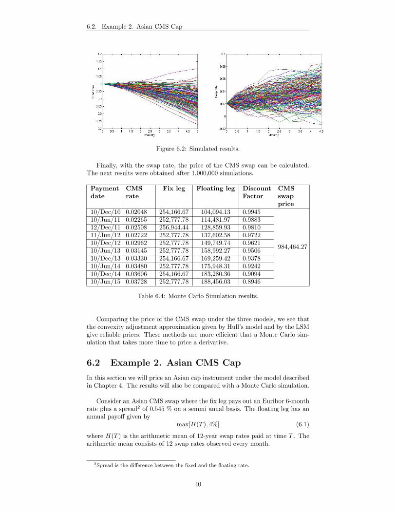
The next two graphs show two hundred discount curves and swap ratesthat were obtained using formula (5.10) and formula (3.4) respectively. Wecan observe that some bond prices are greater than one, which happens whenthe short rate rt is below zero. As illustrated by figure 6.2, in practice, theprobability of this rate being below zero is indeed small.
39
6.2. Example 2. Asian CMS Cap
Figure 6.2: Simulated results.
Finally, with the swap rate, the price of the CMS swap can be calculated.The next results were obtained after 1,000,000 simulations.
Comparing the price of the CMS swap under the three models, we see thatthe convexity adjustment approximation given by Hull’s model and by the LSMgive reliable prices. These methods are more efficient that a Monte Carlo sim-ulation that takes more time to price a derivative.
6.2 Example 2. Asian CMS Cap
In this section we will price an Asian cap instrument under the model describedin Chapter 4. The results will also be compared with a Monte Carlo simulation.
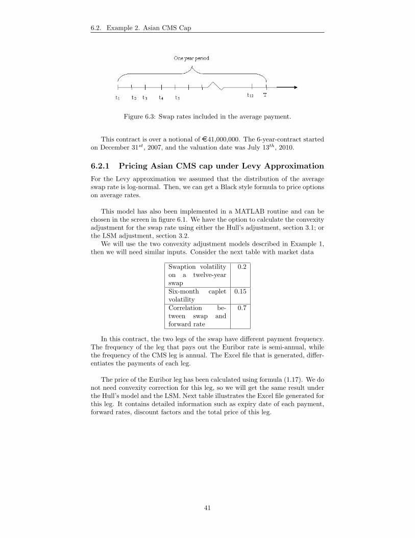
Consider an Asian CMS swap where the fix leg pays out an Euribor 6-monthrate plus a spread2 of 0.545 % on a semmi anual basis. The floating leg has anannual payoff given by
max[H(T ), 4%] (6.1)
where H(T ) is the arithmetic mean of 12-year swap rates paid at time T . Thearithmetic mean consists of 12 swap rates observed every month.
2Spread is the difference between the fixed and the floating rate.
40
6.2. Example 2. Asian CMS Cap
Figure 6.3: Swap rates included in the average payment.
This contract is over a notional of ¤41,000,000. The 6-year-contract startedon December 31st, 2007, and the valuation date was July 13th, 2010.
6.2.1 Pricing Asian CMS cap under Levy Approximation
For the Levy approximation we assumed that the distribution of the averageswap rate is log-normal. Then, we can get a Black style formula to price optionson average rates.
This model has also been implemented in a MATLAB routine and can bechosen in the screen in figure 6.1. We have the option to calculate the convexityadjustment for the swap rate using either the Hull’s adjustment, section 3.1; orthe LSM adjustment, section 3.2.
We will use the two convexity adjustment models described in Example 1,then we will need similar inputs. Consider the next table with market data
Swaption volatilityon a twelve-yearswap
0.2
Six-month capletvolatility
0.15
Correlation be-tween swap andforward rate
0.7
In this contract, the two legs of the swap have different payment frequency.The frequency of the leg that pays out the Euribor rate is semi-annual, whilethe frequency of the CMS leg is annual. The Excel file that is generated, differ-entiates the payments of each leg.
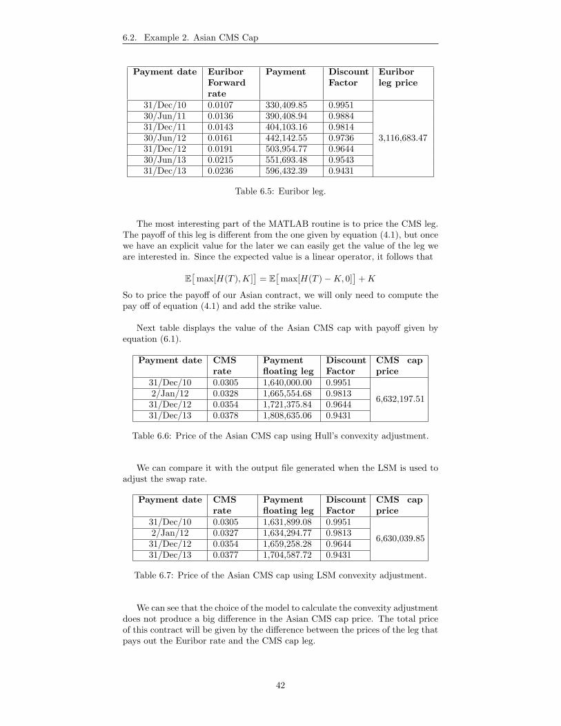
The price of the Euribor leg has been calculated using formula (1.17). We donot need convexity correction for this leg, so we will get the same result underthe Hull’s model and the LSM. Next table illustrates the Excel file generated forthis leg. It contains detailed information such as expiry date of each payment,forward rates, discount factors and the total price of this leg.
The most interesting part of the MATLAB routine is to price the CMS leg.The payoff of this leg is different from the one given by equation (4.1), but oncewe have an explicit value for the later we can easily get the value of the leg weare interested in. Since the expected value is a linear operator, it follows that
E[
max[H(T ),K]]
= E[
max[H(T )−K, 0]]
+K
So to price the payoff of our Asian contract, we will only need to compute thepay off of equation (4.1) and add the strike value.
Next table displays the value of the Asian CMS cap with payoff given byequation (6.1).
Table 6.7: Price of the Asian CMS cap using LSM convexity adjustment.
We can see that the choice of the model to calculate the convexity adjustmentdoes not produce a big difference in the Asian CMS cap price. The total priceof this contract will be given by the difference between the prices of the leg thatpays out the Euribor rate and the CMS cap leg.
42
6.2. Example 2. Asian CMS Cap
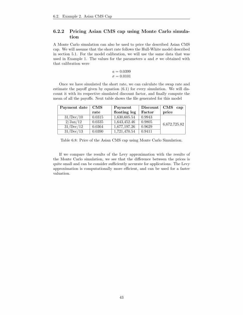
6.2.2 Pricing Asian CMS cap using Monte Carlo simula-tion
A Monte Carlo simulation can also be used to price the described Asian CMScap. We will assume that the short rate follows the Hull-White model describedin section 5.1. For the model calibration, we will use the same data that wasused in Example 1. The values for the parameters a and σ we obtained withthat calibration were
a = 0.0399σ = 0.0101
Once we have simulated the short rate, we can calculate the swap rate andestimate the payoff given by equation (6.1) for every simulation. We will dis-count it with its respective simulated discount factor, and finally compute themean of all the payoffs. Next table shows the file generated for this model
Table 6.8: Price of the Asian CMS cap using Monte Carlo Simulation.
If we compare the results of the Levy approximation with the results ofthe Monte Carlo simulation, we see that the difference between the prices isquite small and can be consider sufficiently accurate for applications. The Levyapproximation is computationally more efficient, and can be used for a fastervaluation.
43
Appendix A
Moments under Black’smodel
The Black’s model can be generalized into a class of models known as log-normalforward models, the main assumption is that the modelled rate at maturity islog-normally distributed. Let Si be the modelled rate. Under the risk neutralmeasure Q, Si is a martingale. The process followed by this rate is given by
dSi(t) = σi(t)Si(t) dW (t) (A.1)
where σi(t) is the instantaneous volatility, and Wi(t) is a standard Brownianmotion under the Q measure . Using Ito’s formula the solution of last equationis
Si(T ) = Si(0)e∫ T0 σi(t)dW (t)− 1
2
∫ T0 σ2
i (t)dt. (A.2)
The stochastic integral∫ T
0σi(t)dW (t) is well defined since σi(t) is a deter-
ministic function. It is normally distributed with mean zero. If∫ T
0σi(t)2dt <∞
then the variance is given by
V ar[ ∫ T
0
σi(t)dW (t)]
= E[( ∫ T
0
σi(t)dW (t))2]
=∫ T
0
σi(t)2dt
where we used Ito’s isometry in the last step.
It is worth noting that the moment generating function of a random variableX that is N (µ, σ2) distributed is given by
E[etX ] = eµt+12σ
2t2 . (A.3)
We will often need to compute the second moment of the log-normally dis-tributed rate Si, that can be written as
EQ[Si(T )2] = EQ[Si(0)2e2
∫ T0 σi(t)dW (t)−
∫ T0 σ2
i (t)dt]
= Si(0)2e−∫ T0 σ2
i (t)dtEQ[e2∫ T0 σi(t)dW (t)
]= Si(0)2e
∫ T0 σ2
i (t)dt.
44
The last equality is an application of (A.3).
If σ is constant, then the expected value becomes
EQ[Si(T )2] = Si(0)2eσ2i T . (A.4)
Another quantity that is frequently used is
EQ[(Si(T )− Si(0))2] = EQ[Si(0)2
(e∫ T0 σi(t)dW (t)− 1
2
∫ T0 σ2
i (t)dt − 1)2]
= Si(0)2(EQ[e2∫ T0 σi(t)dW (t)−
∫ T0 σ2
i (t)dt]
+ EQ[− 2 e
∫ T0 σi(t)dW (t)−
∫ T0 σ2
i (t)dt + 1])
= Si(0)2(e∫ T0 σ2
i (t)dt − 1)
= Si(0)2(eσ
2i T − 1
). (A.5)
And finally, the expectation of the product of two rates is given by
EQ[Si(Ti)Sj(Tj)] = EQ[Si(0)e
∫ Ti0 σi(t)dW (t)− 1
2
∫ Ti0 σ2
i (t)dt
∗ Sj(0)e∫ Tj0 σj(t)dW (t)− 1
2
∫ Tj0 σ2
j (t)dt]
= Si(0)Sj(0)e−12
( ∫ Ti0 σ2
i (t)dt+∫ Tj0 σ2
j (t)dt)
∗ EQ[e∫ Ti0 σi(t)dW (t)+
∫ Tj0 σj(t)dW (t)
].
To compute the last expectation we will use (A.3). Notice that the co-variance between the variables
∫ Ti0σi(t)dW (t) and
∫ Tj0σj(t)dW (t) is given by
σiσj minTi, Tj, when the volatility σi and σj are constants.Then we have
EQ[Si(Ti)Sj(Tj)] = Si(0)Sj(0)e−12 (σ2
i Ti+σ2jTj)e
12 (σ2
i Ti+σ2jTj+2σiσj minTi,Tj)
= Si(0)Sj(0)eσiσj minTi,Tj. (A.6)
45
Appendix B
Detailed derivation ofBlack’s formula to priceoptions
To price a caplet with underlying rate Si(T ) observed at time T , that followsthe Black’s model described in previous appendix, equation (A.1), we need tocompute the expected value of its payoff
EQ[max [Si(T )−K, 0]]
where Q denotes the equivalent martingale measure.
From Equation (A.2), we have that
Si(T ) = Si(0)e∫ T0 σi(t)dW (t)− 1
2
∫ T0 σ2
i (t)dt
= Si(0)em+V y
where m is given by
m = −12
∫ T
0
σ2i (t)dt
and V 2 has the form
V 2 =∫ T
0
σ2i (t)d(t)
the random variable y is standard normally distributed.
Then the expected value can be written as
EQ[max [Si(T )−K, 0]]
= EQ[max [Si(0)em+V y −K, 0]]
=∫ ∞−∞
max [Si(0)em+V y −K, 0]f(y) dy
where f(x) is the normal probability density function.
Note that Si(0)em+V y −K > 0 if and only if
y >− ln
(Si(0)K
)−m
V=: y′
46
then we have
EQ[max [Si(T )−K, 0]]
=∫ ∞y′
(Si(0)em+V y −K)f(y) dy
= Si(0)∫ ∞y′
em+V yf(y) dy −K∫ ∞y′
f(y) dy
= Si(0)1√2π
∫ ∞y′
e−12y
2+m+V y dy −K(1−N (y′)
)= Si(0)em+ 1
2V2 1√
2π
∫ ∞y′
e−12 (y−V )2 dy −K
(1−N (y′)
)= Si(0)
1√2π
∫ ∞y′−V
e−12 z
2dz −K
(1−N (y′)
)= Si(0)
(1−N (y′ − V )
)−K
(1−N (y′)
)= Si(0)N (−y′ + V )−KN (−y′)= Si(0)N (d1)−KN (d2)
where
d1 =ln Si(0)
K + 12
∫ T0σi(t)2dt√∫ T
0σi(t)2dt
and
d2 = d1 −
√∫ T
0
σi(t)2dt.
If σi is constant, then d1 and d2 can be simply be expressed as
d1 =ln Si(0)
K + 12σ
2i T
σi√T
andd2 = d1 − σi
√T .
47
Bibliography
[1] Benhamou, E. (2000), ”A Martingale Result for Convexity Adjustment inthe Black Pricing Model”, London School of Economics, Working Paper.
[2] Benhamou, E. (2000), ”Pricing Convexity Adjustment with WienerChaos”, London School of Economics, Working Paper.
[3] Benhamou, E. (2002), ”Swaps: Constant maturity swaps and constantmaturity Treasury swaps”. Goldman Sachs International.
[4] Brigo, D. and Mercurio, F. (2001), Interest Rate Models Theory and Prac-tice, Springer Finance.
[5] F. Boshuizen, A.W. van der Vaart, H. van Zanten, K. Banachewicz andP. Zareba, (2010), ”Notes for the course Stochastic Processes for Finance,Risk Management Tools”, Vrije Universiteit.
[6] Geman, H., El Karoui, N. and Rochet, J.-C. (1995), ”Changes of numeraire,changes of probability measure and option pricing”, Journal of AppliedProbability, 32(2), 443-458.