Masters Thesis: Testing of fast transfer relay by an EMTP ...

Testing of Fast Transfer Relay

by an EMTP-based Approach

Wenbin Wu

Pro

ject

Rep

ort

Testing of Fast Transfer Relay by an

EMTP-based Approach

By

Wenbin Wu

In partial fulfilment of the requirements for the degree of

Master of Science in Electrical Sustainable Energy

at the Delft University of Technology, To be defended publicly on Monday, 16 July 2018 at 10:00 AM

Supervisor: Dr. Dipl-Ing Marjan Popov, TU Delft- IEPG

Thesis Committee: Prof. Ir. Mart van der Meijden, TU Delft- IEPG

Dr.Ir. Mohamad Ghaffarian Niasar TU Delft-DCSECS

Ir. Steven.A.de Clippelaar DOW Energy System Technology Center (ESTC)

An electronic version of this thesis is available at http://repository.tudelft.nl/

http://staff.tudelft.nl/en/M.A.M.M.vanderMeijden/

https://www.tudelft.nl/staff/m.ghaffarianniasar

http://repository.tudelft.nl/

Abstract

Industries such as chemical companies need a continuous power supply and the fast transfer

relay Siemens 7uv68 is designed to transfer from present feeder which encounters a fault to an

auxiliary feeder and minimizes the transient torque of the induction motors during transfer.

The relay will be installed in a DOW power plant in South Tarragona, and it should be

validated that the relay can operate well in all kinds of fault scenarios and no mal-operation

would occur in such power plant.

To perform the relay testing, first, the fault signals which reflect the dynamic performance

of DOW Tarragona are generated by ATP-EMTP. The EMTP model of the DOW power plant

has two main parts: the Tarragona power plant with auxiliary relays (overcurrent 50/50N,

differential 87T) which send tripping and blocking command to 7UV68. Besides, in order

to track the frequency and phase deviation between auxiliary feeder bus and the motor

bus during transfer and configure a proper setting of the relay, the frequency measurement

is accomplished by a zero-crossing method and the phase angle is measured by Clarke

transformation. The test setup is made by 2 Omicron Amplifiers and a PLC which is used to

simulate breakers’ behavior for main-tie configuration.

Based on the testing requirements, the relay settings are tuned to ensure the motor bus

transfer can be initiated by all kinds of faults in feeder bus, and the relay is blocked when

faults occur in motor bus. .Besides, the motor bus can also be transferred to the auxiliary bus

when a fault occurs in transmission grid with the help of relay self-start function.

Furthermore, the trip delay of differential relay 87T and the communication delay affects the

transfer time and the transfer inrush behaviors.

Keywords: ATP-EMTP, Mot Bus Transfer, Frequency Tracking, Induction Motors,

Transient torques, Fast transfer relay, Industrial Plant Protection

Table of Contents

Acknowledgements viii

Glossary x

1 Introduction 1

1-1 Background and Introduction . . . . . . . . . . . . . . . . . . . . . . . . . . . . 1

1-2 Literature Review . . . . . . . . . . . . . . . . . . . . . . . . . . . . . . . . . . 2

1-3 Objectives . . . . . . . . . . . . . . . . . . . . . . . . . . . . . . . . . . . . . . 3

1-4 Research Methodology . . . . . . . . . . . . . . . . . . . . . . . . . . . . . . . 4

1-5 Thesis Layout . . . . . . . . . . . . . . . . . . . . . . . . . . . . . . . . . . . . 4

2 Basic Theory of Fast Transfer 7UV68 6

2-1 Introduction . . . . . . . . . . . . . . . . . . . . . . . . . . . . . . . . . . . . . 6

2-2 Motor Behaviors during Motor Bus Transfer . . . . . . . . . . . . . . . . . . . . 6

2-3 Basic Transfer Scheme .................................................................................................... 10

2-4 Introduction of Fast Transfer 7UV68 ............................................................................. 13

3 Network modelling in DOW Tarragona South 14

3-1 Introduction ....................................................................................................................... 14

3-2 Network Description ......................................................................................................... 14

3-3 Transmission and Distribution Network Modelling ....................................................... 16

3-3-1 The 230kV Transmission System Modelling ...................................................... 16

3-3-2 Cable Modelling .................................................................................................... 16

3-3-3 Transformer Modelling ......................................................................................... 17

3-4 Electrical Load Modelling ................................................................................................. 19

3-4-1 Static Load and Capacitor Modelling ................................................................ 20

3-4-2 Induction Motor Modelling ................................................................................. 20

Table of Contents iii

3-4-3 Synchronous motor modelling .......................................................................... 27

3-5 Measurement Instrument Modelling ............................................................................. 30

3-5-1 Voltage Transformer Modelling.......................................................................... 30

3-5-2 Current Transformer Modelling .......................................................................... 31

3-6 Auxiliary Relay Modelling and Configuration ................................................................ 33

3-7-1 Simplification for Relay Modelling ..................................................................... 33

3-7-2 Differential Relay Modelling ............................................................................... 33

3-7-3 Instantaneous Overcurrent Relay Modelling ................................................... 35

3-8 Motor Bus Residual Voltage Tracking ................................................................................. 37

3-8-1 Voltage Frequency Tracking .................................................................................... 38

3-8-2 Voltage Amplitude and Phase angle Tracking ..................................................... 38

4 Testing Setup Design 42

4-1 Introduction ...................................................................................................................... 42

4-2 Simulation Results Recording .............................................................................................44

4-3 Test Signals Generation .................................................................................................. 44

4-4 Breaker Time Delay Imitation ........................................................................................ 45

5 Relay Testing 51

5-1 Introduction ....................................................................................................................... 51

5-2 Test Requirement and Test Cases Design ..................................................................... 51

5-2-1 Test Requirement ................................................................................................. 51

5-2-2 Test Cases Design ............................................................................................... 53

5-3 Relay Configuration and Testing for Feeder Bus and Motor Bus Fault ........................ 54

5-3-1 Motor Bus Residual Voltage Behavior after Losing Power ................................. 54

5-3-2 Relay Setting Configuration ............................................................................... 56

5-3-3 Relay Testing Based for Feeder or Motor Bus Fault ........................................... 64

5-4 Relay Configuration and Testing for Transmission Grid Fault ........................................ 64

5-5 Sensitivity Testing on Differential Relay Trip Delay ......................................................... 65

5-6 Sensitivity Testing on Communication Delay .................................................................... 69

6 Conclusion and Future Work 70

6-1 Conclusion ........................................................................................................................ 70

6-2 Future Work ................................................................................................................................... 71

A Test Setup 72

B System Data of DOW Tarragona 73

C Model for Auxiliary Relay and Additional Measurement 75

Table of Contents iii

D The relay setting of 7UV68 80

E EMTP Modelling For Starting a Synchronous Motor 85

F Basic Testing for Simultaneous Transfer Sequence 87

iv Table of Contents

List of Figures

1-1 Motor Bus Transfer System with Main-Tie Configuration .............................................. 2

2-1 The schematic diagram of induction motor [15]............................................................ 7

2-2 Illustration of Residual and Reference Voltage .................................................................. 10

2-3 Illustration of Different Transfer Modes .......................................................................... 12

2-4 Rate Input of the relay 7UV68 [16] ................................................................................... 13

3-1 The Transmission Network in DOW South Tarragona ......................................................... 15

3-2 The Distribution Network in DOW South Tarragona ........................................................... 15

3-3 The Short Circuit Level of 230kV Transmission Grid ...................................................... 16

3-4 The Short Circuit Level of 230kV Transmission Grid .................................................. 17

3-5 Simulated Short Circuit Level in 230kV Bus ..................................................................... 17

3-6 Input Data of BCTRAN Transformer Model ................................................................... 19

3-7 Short Circuit in TP Low Voltage Side............................................................................... 19

3-8 The Static Load Model and Result Validation .................................................................... 20

3-9 The Typical Data of Industrial Induction Motors ......................................................... 21

3-10 The Induction Motor Parameters Estimation ................................................................. 21

3-11 The Torque and Current Graph with a Slip change ........................................................ 22

3-12 Representation and Input Data of Induction Motor in EMTP ......................................... 23

3-13 The Induction Motor Model ............................................................................................ 24

3-14 The Load Curve Fitting of Typical Industrial Rotary Pump ............................................ 25

3-15 The Speed and Torque Curve of the Induction Motor ......................................................... 25

3-16 Speed and Stator Current during Motor Start-up ........................................................ 26

3-17 Stretch of Synchronous Motor [15] ...................................................................................... 27

3-18 Input Data in ATP-EMTP ........................................................................................................ 28

3-19 Excitation Behavior for Different Fault ................................................................................ 29

vi List of Figures

3-20 The Illustration of a Compressor [17]............................................................................... 30

3-21 The Load and Stator Current of Synchronous Motor MC331 ..................................... 31

3-22 The Equivalent Circuit of VT...........................................................................................32

3-23 The EMTP Model of Voltage Transformer .......................................................................... 32

3-24 The Equivalent Circuit of Current Transformer ................................................................ 33

3-25 The Non-linear Magnetizing Curve ................................................................................ 33

3-26 The CT Model in EMTP ................................................................................................... 34

3-27 The Fault Current Contribution from All Motors ............................................................... 37

3-28 Simulation of Single Phase Fault in 25kV Motor Bus ................................................... 38

3-29 Illustration of Zero Crossing Method ............................................................................ 38

3-30 Frequency Measurement of Voltage Signal .................................................................. 39

3-31 Voltage Amplitude and Phase Angle Difference under symmetrical condition ............40

3-32 Voltage Amplitude and Phase Angle Difference under unsymmetrical condition...41

4-1 The Overall Testing Setup .............................................................................................. 42

4-2 Analog and Binary Signals Sending to the Relay 7UV68 ............................................ 42

4-3 The OCC Test Library for Different Fault Scenarios ....................................................... 43

4-4 Basic Technical Data of Two Amplifiers ........................................................................ 44

4-5 Time constant of breakers during opening .................................................................. 45

4-6 Time constant of breakers during closing .................................................................... 46

4-7 Connections of LOGO PLC................................................................................................. 47

4-8 Ladder Diagram of PLC ................................................................................................... 48

4-9 Simulation of PLC Ladder Graph ................................................................................... 49

5-1 The sketch of Tarragona power plant .......................................................................... 51

5-2 The Voltage Magnitude and delta phase angle for inadvertent breaker opening...54

5-3 The stator current and speed behavior of induction motor in single phase fault...55

5-4 The CFC logic of Load Shedding Function ....................................................................... 56

5-5 Relay Operation Sequence for 25kV single phase Fault ................................................. 56

5-6 Delta Phase Angle Recording for 25kV single phase Fault ............................................. 57

5-7 Comparison of Inrush Torque by Two Transfer Modes ............................................... 57

5-8 Comparison of delta phase angle by Two Transfer Modes ......................................... 58

5-9 Maximum Inrush torque of motors for 25kV LN Fault ..................................................... 58

5-10 Motor Bus Transfer Time Based on Fault Type and Location ..................................... 60

5-11 Maximum Inrush Torque for 25kV side fault ................................................................ 61

5-12 Maximum Inrush Torque for 230kV side fault .............................................................. 61

5-13 The Changed Setting from Suggested Values for self-Start ........................................ 62

5-14 Sensitivity Study of Relay Trip Time ............................................................................. 66

5-15 Sensitivity Study (Inrush Torque) of Relay Trip Time ................................................... 67

5-16 Sensitivity Study of Communication Delay.....................................................................68

Vii List of Figures

5-17 Sensitivity Study (Inrush Torque) of Communication Delay ......................................... 69

Viii List of Tables

List of Tables

3-1 The Transformer Data ....................................................................................................... 19

3-2 The Relationship between mechanical and electrical parameters in universal motor model .............................................................................................................................................. 25

3-3 Load Data of Four Synchronous Motor .................................................................................. 27

3-4 The Parameters of Voltage Transformer ................................................................................ 32

4-1 Basic Technical Parameters of Basic Module and Expansion Module of PLC...............46

4-2 Truth Table of Breaker State ............................................................................................. 47

4-3 Truth table of SR Flip-flop ................................................................................................ 48

5-1 Test List for Feeder Fault .......................................................................................................... 54

5-2 Voltage Amplitude and Delta Phase Angle After Fault ....................................................... 56

5-3 Blank Time for Transmission Grid Fault ............................................................................ 65

5-4 Transfer Mode and Transfer Time for Transmission Grid Fault .................................. 65

Acknowledgements

First of all, I would like to give the greatest gratitude to my supervisor Dr. Dipl-Ing. Marjan

Popov who helped me during the whole period I worked on my master thesis. Besides, I

would like to express my sincere thanks to Steven A. de Clippelaar from DOW for

providing countless academic guide.

Besides, great thanks are going to my family. Without your support, it was impossible for

me to go so far. Finally, I thank all my friends in Delft. I will never forget the colourful

days in Delft.

Delft, University of Technology Wenbin Wu

July 5, 2018

“Whatever is reasonable is true, and whatever is true is reasonable.”

— Georg Wilhelm Friedrich Hegel

Nomenclature

resU : Motor bus residual voltage after an open-circuit

refU : Feeder voltage of the auxiliary bus which acts as a reference for motor transfer

diffU : Voltage difference between motor bus residual voltage and the reference voltage

df : Frequency difference between motor bus residual voltage and the reference voltage

d : Phase angle difference between motor bus residual voltage and reference feeder voltage

lT : Torque of mechanical loads

r : Rotor speed of motors

diffI : Differential current of differential relay 87T

ResI : Restraint Current of differential relay 87T

sU *

sU *

0U : The representation of three phase voltage in space vector domain

aU bU cU : Instantaneous voltages in abc frame

U U : Two perpendicular signals transferred by Clarke Transformation

aI bI cI : Instantaneous currents in abc frame

0I : Zero Sequence Current

rdcI : DC current induced in rotor winding when motor loses power supply

: Load Angle of Synchronous motor

Glossary

ATP-EMTP Alternative Transient Programs- ElectroMagnetics Transient Programs

MBT Motor Bus Transfer

ABT Automatic Bus Transfer

CB Circuit Breaker

OCC Omicron Control Centre

DFT Discrete Fourier Transformation

IO Input and Output

ANSI American National Standards Institute

MMF Magnetic Motive Force

PLC Programmable Logic Controller

RDFT Recursive Discrete Fourier Transformation

HSBT High Speed Bus Transfer

RTDS Real-time Digital Power System Simulator

GTAO Gigabit Transceiver Analogue Output

GTFPI Gigabit Transceiver Front Panel Interface

Chapter 1

Introduction

1-1 Background and Introduction

A typical chemical plant relies heavily on electricity to supply mechanical equipment, drive

electrochemical processes, and implement process controls. The majority of electrical loads

in the chemical industries for instance DOW are induction motors which serve for the pumps,

fans as well as compressors.

In the absence of protection and control equipment, a power blackout would lead to an

uncontrolled shutdown of the process operations. If the process operation involves large

quantities of hazardous chemicals, an uncontrolled shutdown can release hazardous

chemicals with catastrophic consequences and even contributes to severe explosions.

Statistics indicate that electrical faults account for 7%-11% of accidents for chemical

industries [1]. A severe blackout may contribute to the losing speed of all motors and the

failure of all control units such as PLC and SCADAs. Consequently, it is crucial that a

chemical company should maintain the continuity and increase the reliability of power

supply.

In order to ensure the reliability of such electrical power plant, a network with an auxiliary

power supply is designed (main-tie configuration). During the fault, motor buses require a

transfer from a present feeder to an auxiliary feeder. A simplified diagram of the motor bus

transfer (MBT) system is shown in figure 1-1.

2 Introduction

Figure 1-1: A Motor Bus Transfer System with Main-Tie Configuration

The motor bus transfer (MBT) schemes are employed to maintain the continuity in processes

served by aggregates of motors. Following an event such as the generator trip, all the

motors which connect with the feeder bus are disconnected from their main power source

and shift to the auxiliary bus (healthy feeder). However, if there is no intelligent electronic

device to control such transfer, the re-closing of the breaker in the auxiliary bus would

contribute a large inrush current and torque which reduces the lifetime of all motors. Based

on that, the fast transfer (high speed bus transfer) relay has been designed. Such relay has

some significant benefits: the disruption (transfer time) is quite short to ensure the

continuous operation of the critical loads, and more importantly, the fast transfer relay can

decrease the large transient current and torque of induction motors when a motor transfer

happens. The secure transfer is realized by monitoring the difference of voltage magnitude

diffU , phase angle d and frequency df between motor bus and feeder bus. If those three

parameters fulfill particular thresholds, the breaker of the healthy feeder (auxiliary feeder)

will close and motors are transferred successfully.

1-2 Literature Review

The bus transfer system has been analyzed and employed for a long period of time and the

first research paper on motor bus transfer was published in 1950 by Lewis and Marsh [2].

They gave a basic understanding and modelling of a bus transfer based on statistically

analyzing the behavior of motors. Walter [3] indicated that the first 0.5s are the most critical

time period for bus transfer by determining the auxiliary bus voltage and angle from the

dynamic equivalent circuit of a single motor. Yeager [4] presented the result of multi-motor

transfer behaviors in several conditions by transient stability analysis method. Beckwith and

Hartmann [5] in 2005 used an experimental way to analyze the voltage behavior of motor

bus during transfer and suggested that the decaying rates of the residual voltage magnitude

and frequency depend on various factors including the type and size of the motors, combined

3 Introduction

inertia and open-circuit time constant of the motors, and motor loads.

After the 2000s, more research was focused on the automatic bus transfer (ABT) system

design. Murty [6] from Beckwith electric company addressed the design of both hardware and

transfer algorithm of a high-speed motor bus transfer relay. That paper elaborated the

motor bus transfer scheme which includes fast, in phase and residual transfer mode and

proposed an adaptive time window Discrete Fourier Transform (DFT) algorithm for both

frequency and phase angle measurement. This was realized by changing the sampling rate

and decreasing the error of conventional DFT method when frequency deviates from the

nominal value.

As illustrated in chapter 1-1, the frequency should be measured continuously after the breaker

in fault bus trips to ensure a successful motor transfer and therefore, many researchers

developed different frequency measurement method. The most intuitive method for

frequency tracking is zero-crossing where the frequency is measured based on the time

interval of two zero crossing point [7]. However, such method will lose frequency

information during one measurement circle, and Begovic [8] designed a modified method to

enhance the accuracy. E. Aboutanios [9] adopted Clarke transformation which represented

the three-phase single by one phasor and decomposed such vector into 2 orthogonal planes to

track the frequency. V.Eckhardt [10] proposed a method which use PLL (Phase Lock loop) to

track the frequency, which can achieve high accuracy in quasi-steady state. However, the time

delay of the PI controller introduces measurement error in dynamic measurement with steep

frequency changes. Furthermore, Pony method and Smart DFT method were elaborated

by J.Z.Yang [11] and T. Lobos [12] for more accurate frequency tracking with existing of

high order harmonics, but such method requires a high computational complexity and RAM

storage.

Except for the scientific study, industries have also developed some standards for motor

transfer. The ANSI (American National Standards Institute) published standards in 1978 for

fast transfer criterion C50.41-2000 [13] which suggests that the resultant voltage vector per

frequency diffU

freq (the voltage phasor difference between motor bus and incoming bus divided

by instantaneous frequency) should not exceed 1.33 PU. The testing of the MBT relay was

shown by Thomas R. [14]. The Beckwith relay has been tested, and the relay setting has

been proposed for general power plants. Case studies of a number of live MBTs were

presented and analyzed, and finally, a transfer metric has been shown based on the transfer

mode and transfer time.

1-3 Objectives

Although a lot of research has been done for the motor bus transfer, most of those studies were

mainly focused on the transient simulation of the system. Only a few papers are referred to

the fast Transfer relay testing. However, the fast relay testing only gave the general result

based on simple testing cases instead of the fault recording from power system simulations.

Besides, the previous testing designed by other engineers only focused on the transfer mode

and transfer time of the fast transfer relay and gave no testing results about transient torque

behavior of motors controlled by the relay. Hence, this thesis combines both relay testing of

Siemens fast transfer relay and transient torque behavior analysis of induction motors by

4 Introduction

building EMTP models of the DOW Tarragona.

The research objectives of the thesis are listed as follow:

1. Studying and understand the basic theory of fast transfer relay;

2. Building an EMTP model for the testing signals generation and system dynamics study;

3. Designing the testing setup for fast transfer relay testing;

4. Selecting a proper setting of the fast relay 7UV68 and test the relay based on the testing requirements.

1-4 Research Methodology

The whole project is performed in 4 steps. First, the basic transfer scheme and theory should

be analyzed to make preparation for the system modelling and testing setup design. Then,

in order to have the analog signals (voltage and current signal) and binary signals (breaker

position and auxiliary input) which act as the relay input, the power system of DOW South

Tarragona with protection relays (over-current and differential relays) need to be modelled

and configured in ATP-EMTP to get different dynamic fault signals. Third, the testing setup

should be developed with a combination of software (Omicron Control Center) and hardware

(Omicron CMC356, CMS156, Siemens Logo PLC) configuration. Finally, the testing results

(transfer time and transfer modes) recorded by Omicrons will be re-applied to the EMTP

simulation to analyze the transient inrush torque of all induction motors a when the breaker

in reference feeder closes.

1-5 Thesis Layout

There are six chapters in this thesis:

Chapter.1: Introduction:

This chapter addresses the importance of fast transfer relay for industries and highlights the

previous studies about the fast transfer system. Then the objectives of the thesis are

introduced, followed by the thesis layout.

Chapter.2: Basic theory of fast transfer:

This chapter gives a brief illustration of fast transfer relay. First, the motor behavior when

losing power supply is analyzed by the space vector method, followed by the introduction of

typical transfer scheme of motor transfer relays. Finally, the Siemens fast transfer relay

7UV68 is introduced.

Chapter.3: DOW Tarragona power plant modelling:

This chapter mainly illustrates the power plant modelling in DOW Tarragona. First, the

power network including electrical loads, transmission and distribution grids is modelled.

Then, to acquire suitable analog and binary signals for the fast transfer relay testing, the

measurement instruments and auxiliary relays are modelled. Finally, to analyze the testing

results, the real-time amplitude, phase angle and frequency of voltages in both motor bus and

reference feeder bus are measured.

5 Introduction

Chapter.4: Testing Setup Design:

This chapter focuses on the testing setup design for fast transfer relay testing. The hardware

setup and software configuration of the testing are illustrated in detail.

Chapter.5: Fast transfer relay testing:

This chapter elaborates detailed testing results of fast transfer relay based on the EMTP

model of DOW Tarragona. In this chapter, the test requirements are shown at the

beginning. Next, the relay settings based on the testing requirements are configured. The

testing results including the transfer mode, the transfer time and the inrush torque of each

fault scenarios are shown in this chapters. Finally, sensitivity testing on both tripping delay

of 87T and communication delay are proposed, and the most severe cases for motor bus

transfer can be examined.

Chapter.6: Conclusion and Future Work

This chapter makes an overall conclusion based on previous chapters and gives

recommendations for future research.

Chapter 2

Basic Theory of Fast Transfer 7UV68

2-1 Introduction

When talking about a fast transfer relay, two things should be clear: what is the motor bus

transfer and why the fast transfer relay is needed. As the brief introduction in chapter 1

shows, motor bus transfer relays transfer all motors from fault feeder to the healthy bus, but

why it is not possible to transfer the motors by manually open the fault feeder and close the

auxiliary feeder. This chapter elaborates the significance of fast transfer relay by showing the

motor behaviours during transfer. Besides, an introduction about the testing object,

Siemens fast transfer relay 7UV68 in this thesis will be introduced.

2-2 Motor Behaviors during Motor Bus Transfer

In industry companies such as DOW, a majority of mechanical loads are pumps driven by

induction motors. As figure 1-1 shows, when feeder 1 encounters contingencies such as a

single phase fault, the breaker CB1 should trip to cut the fault from the source. Therefore,

all induction motors will lose power supply. It is essential to understand the motor behavior

in such open circuit period.

To simplify the problem, we only consider the condition where a single induction connects

to an infinite bus. As the schematic of induction motor shows (figure 2-1), typical induction

motors have two winding groups stator windings and rotor windings. The three windings

phase have a 120

shift in space. When a symmetrical 3 phase AC voltage applies to such

three phase windings, a rotating magnetic field will be generated. The relative movement

between rotating magnetic motive force F1 and rotor windings induces a current in rotor

winding. With the help of the rotating field and induced current, the induction motors can

generate torques.

7 Basic Theory of Fast transfer 7UV68

If the power source of a single induction motor trips, the stator current of the motors

disappears immediately, and the MMF (magnetic motive force) SF generated by stator

current disappears simultaneously. However, based on the magnetic theory, the magnetic

flux density B generated by three-phase current cannot change immediately. Therefore, to maintain the magnetic flux density, the rotor winding should induce a DC current which compensates the vanishing of stator current.

Figure 2-1: The schematic diagram of the induction motor [15]

Some books and studies [5] [15] indicate that the DC rotor current decays by the rotor

winding time constant /r r rT L R . The MMF generated by the decaying DC rotor current rF

has a relative rotation speed r (mechanical speed of rotor) with the stator. Therefore, the

stator winding can induce a voltage called motor residual voltage resU . When the motors lose

power supply, the air gap torque of the motor becomes to zero as there is no electrical power input. Therefore, the rotation speed will decrease because of the drag force of the mechanical

load. With the decaying amplitude of the dc rotor current rdcI and rotor rotation speed r ,

the amplitude and frequency of motor residual voltage will decay. However, until now, there are no anayltical solutions for the motor behavior after an open circuit of a running motor. Therefore, this thesis derives the anayltical solutions for an open-circuit of a single motor.

Some assumptions should be made before solving those equations: the magnetic saturation and eddy current are neglected. In order to represent the three phase voltages by one parameter, a space vector method has been developed in the book [15]. The three-phase voltages in abc domain are converted into the space vector coordinate by equation 2-1.

2

* 2

12

13

1 1 1

2 2 2

a

b

c

a a u

a a u

u

s

s

s0

u

u

u

(2-1)


In equation 2-1,120ja e

,2 240ja e

are the constants of space vector transformation. The

instantaneous voltage au , bu and cu are converted to voltage space vector su . *

su is the

conjugate of the voltage vector su and can be ignored. *

s0u is the zero sequence voltage which

can be neglected in symmetrical conditions.

Based on the same transformation, we can convert the current and flux linkage in the space vector domain. Based on Faraday’s law, we can have both the rotor and stator voltage equation in space vector domain:

s

r

dR

dt

dR

dt

ss s

rr r

Ψu i

Ψu i

(2-2)

Where sΨ and rΨ are flux linkages in stator and rotor winding.

Such flux linkages are calculated by self-inductance and mutual inductance.

j

s m

j

r m

L M e

L M e

s s r

r r s

Ψ i i

Ψ i i (2-3)

Where mM is the mutual inductance between rotor and stator; sL and rL are the self-

inductance of stator and rotor respectively; is the angle difference between the rotating

rotor frame and stator frame which is equal to rt ; r is the mechanical speed of the

motor.

If we convert the rotor side parameters into the stator frame then we have:

'

'

'

j

r r

j

r r

j

r e

e

e

e

u u

i i

(2-4)

Where the'

ru ,'

ri ,'

r represent the rotor quantities in the stator frame.

Applying equation 2-4 to 2-2 and 2-3 respectively, we can have the voltage and flux linkage

equation respectively:

'' '

'

' '

s

rr r

r

r

r

m s

r

s m

s r

dR

dt

d

M

dt

M

R j

L

L

ss s

s s

Ψu i

Ψu i Ψ

Ψ i i

Ψ i i

(2-5)


If the power supply is tripped, the three-phase current becomes 0, which means 0si , and

since the rotor winding is short-circuited (rotor voltage is zero), ' 0ru and equation 2-5

changes to:

'

0 r r

im

r

d

dt

dR j

dt

s

r

Ψu

Ψi

(2-6)

Suppose the motor was tripped at 0t , and the rotor current at that moment is 0rtI . Based on

the first order response of LR circuit, current flows the rotor can be derived as:

0

0

'

t t

jTrrtI e e

r

i (2-7)

Where r

r

LTr

R is the time constant of rotor winding (a RL circuit).

Combining equation 2-6 and 2-7, we can have the analytical solution of residual voltage for

a single induction motor: 0

0

1( )r r

t t

T j t

m dc rM I e jw eTr

im

u (2-8)

Based on the equation 2-8, the amplitude of motor residual voltage for single induction

motors is proportional to the mutual inductance of rotor and stator mM , the time constant

of the rotor winding rT as well as the rotor speed r . The complex notation rj te

indicates

that the voltage vector is rotating is in the space vector coordinate with a rotating speed r

. Therefore, the frequency of the residual voltage in abc coordinate depends on the rotating

speed.

At the mechanical side, if we assume that the inertia of the induction motor is J , the friction

constant is D , and the load torque LT ,we can have:

0rL r

dJ T D

dt

(2-9)

From equation 2-10 we can see that the inertia and mechanical load impacts the rotating

speed. High motor inertia and low mechanical load contributes to a slow rotor speed

decaying and consequently leads to a slow decaying of voltage frequency.

However, for synchronous motors which have a constant excitation loop, we will have a

different expression of motor bus residual voltage. For a synchronous motor with a constant

excitation, during the open circuit period, we have equation 2-10, where fI is the constant

excitation current: ' j

fI e ri (2-10)

Applying 2-11 into 2-7, we have:

( ) rj t

m f rM I j esmu (2-11)


From equation 2-11 we can conclude that the magnitude of the motor residual voltage of

synchronous motors will also decrease with the respective of decaying rotating speed.

However since the excitation current fI is constant for a synchronous motor, the

attenuation 0t t

Tre

disappears.

Therefore, we can conclude that the residual voltage of a single synchronous motor will

decrease slowly than the induction motor. Based on that, the magnitude of residual voltage

in a motor bus with both synchronous motors and induction motors delays slower than

purely induction motors.

For some power plants such as DOW Tarragona, the induction motors and static loads are

connected to the same bus. When losing power supply, the inductions motors generate a

residual voltage, and therefore, the static load is supplied by the motor bus residual voltage

resU, and the current will flow from the motor groups to the loads. In such cases, the

induction motors act as generators and supply electrical power to the static loads. Based on

the law of conservation of energy, the electrical power flows through such loads must be

converted from the remaining flux, which leads to further decay of flux. Therefore, the

residual voltage will decay fast when connecting a static load.

The analytic way is only suitable for a single motor and numerical ways are used to simulate

the motor residual voltage with more motors. In this thesis, we use ATP-EMTP to simulate

the motor bus residual voltage for mutli-motors with loads (chapter 3).

2-3 Basic Transfer Scheme

For motor bus transfer, both the motor bus residual voltage resU and the feeder bus voltage

refU which acts as the reference for transfer should be measured. Equation 2-8 and 2-11

indicate that both the magnitude and frequency of the residual voltage in motor bus decays.

The decaying of frequency contributes to a fast changing of phase angle. Figure 2-2 indicates

the phasor diagram of motor bus residual voltage and the reference voltage.


Figure 2-2: Illustration of Residual and Reference Voltage

Suppose at the instant 0t , the breaker opens (no fault occurs before breaker opens), then the

root of residual voltage phasor follows the blue line, with a changing magnitude and initial

phase angle. Consequently, the rotating residual voltage phasor resU and stationary reference

voltage phasor in auxiliary feeder refU may lead to a voltage difference diffU which is also

called resultant voltage. When motors transfer from fault feeder to auxiliary feeder, the voltage difference contributes to a large inrush current which is usually 8-12 times higher than nominal motor current. [5] The large current may lead to overheating of the stator winding and a large inrush torque which damages the motors’ mechanical structure and eventually curtails the lifetime.

To decrease the inrush current and current and limit the damage to the motors, the American

National Standards Institute (ANSI) standard C50.41-2000 claims that the resultant voltage

should follow the criterion below: 1.33( / )diff

PU Hzfreq

U .

Here 1 PU represents the nominal line to line voltage of the motor.

Based on the ANSI regulations, an intelligent device called fast transfer relay is designed.

Before talking about the motor bus transfer modes, the breaker switching sequence which

plays a significant role in the motor bus transfer should be analyzed. Breaker switching

sequence means the operating sequence of running source breaker and an alternative feeder

breaker during the whole transfer

Typically, there are three kinds of transfer sequences: parallel sequence, simultaneous

sequence and sequential sequence.

1. Parallel Sequence

In parallel sequence transfer, the auxiliary source is already connected to the motor bus

before the fault bus is tripped. The aim of the parallel sequence is to initiate a transfer of

all motors without any interruption, so there would be an over-leaping period when both the


two feeder sources connect to the motor bus. However, there would be a small voltage angle

difference between two sources. Therefore, a parallel connection of two power source leads

to a circulation of power flow in steady state. Besides, the parallel sequence transfer has

another significant shortcoming. Once there is a fault, the fault would be fed by both two

sources during the over-leaping period which results in an increase of short-circuit current

and instability of power system. In practice, such mode is only used for synchro-check of

two feeders.

2. Simultaneous Sequence

As the name indicates, in a simultaneous transfer scheme, the trip command is sent to the

breaker in faulty feeder, and at the same time, the close command is sent to the breaker in

the auxiliary bus. Theoretically, this breaker sequence is the best since there is no blank time

that all motors lose power supply for such scheme. In addition, there is no fault feeding from

the auxiliary bus. However in practice, if the breaker at the faulty bus takes more time to

open (usually occurs due to the arc) or refuse to open, the simultaneous closing of the

breaker in auxiliary bus contributes to a fault feeding from two sources and leads to a severe

problem. Appendix F shows the parallel operation of two sources when the fault time is

longer than the breaker closing time during the simultaneous seqeunce. Besides, appendix

F also supplies some basic testing result based on DOW’s request.

3. Sequential Sequence

In sequential transfer, the auxiliary source only connects to the motor bus after the tripping

of the faulty bus. Sequential sequence deliberately avoids the parallel operation of the two

source and will have a blank time that motors lose power supply. In order to avoid the

parallel operation of two power sources, the sequential sequence with a more conservative

breaker transfer scheme is chosen in this thesis.

Based on the sequential sequence transfer sequence, the fast transfer relay supplies the

following transfer modes:

1. Fast Mode

From figure 2-2, we can see that after the breaker trips, the phase difference and voltage

amplitude difference | |diffU are quite small at the first 10-100ms. Therefore, the fast

transfer scheme attempts to decrease the delta phase angle between feeder bus and motor

bus d by minimizing the motor tripping time before transferring to an auxiliary bus. The

fast transfer mode requires high speed and accurate phase angle measurement algorithm.

Based on the factory testing [16], Siemens proves that when the boundary of the delta phase

angle is about 60,

diffU

freq is less than 1PU/Hz. Considering the breaking time of the breaker

(usually 50ms), Siemens suggests that the threshold of delta phase angle should be about

20to 40

and the real-time delta frequency df should be set as 1.0 to 2.0 Hz. As the relay

needs time to analyze the faulty signals, the shortest action time is one electrical cycle

(20ms). The fast mode is only valid for the first 120ms. A time expiration leads to other

transfer modes.

2. Real-time Fast Mode

If fast mode fails (usually most fault cases cannot fulfill the fast mode threshold), then the

relay automatically goes to a real-time fast mode. This mode extends the threshold of the


delta phase angle d to 90 meanwhile the resultant voltage per frequency

diffU

freq should be

less than 1.33PU/Hz. Besides, the typical setting value of frequency difference fd ranges

from 3Hz to 6Hz.

3. In Phase Mode

If fast transfer and real-time fast mode fail, the device can turn into in-phase transfer mode.

As the name indicates, the motor bus residual voltage is almost in phase with the reference

voltage, which is pretty good to decrease the inrush current. The typical value of the phase

angle difference d is set from 5

to 10

and the typical setting of the delta frequency df is

range from 5Hz-10Hz.

4. Residual Voltage Mode

If in-phase mode fails, then the relay would change to the residual voltage mode. In this

mode of transfer, the motors are transferred if the amplitude of the motor bus voltage uA

reaches a low value to prevent motor damage. However, it takes a very long time for the motor

bus residual voltage to decay to a low value. In this case, we do not care about the phase angle

difference since the magnitude of the motor bus voltage is relatively low. The typical setting

of uA is from 0.2 PU to 0.3 PU. However, it is crucial for motors transferring in this mode,

as in such transfer mode, the motor speed would be quite low and stalling would occur for

system with a very low inertia. Besides, the long transfer time (typically 300-600ms) would

interrupt the continuous chemical process.

5 Long-Time Mode

If all previous modes fail due the to the software or hardware problem of the relay itself

(usually not possible), the long-time mode which acts as the final backup would be initiated

and the system will transfer to the auxiliary bus after 2s. The figure 2-3 summarize all

transfer modes:

Figure 2-3: Illustration of Different Transfer Modes


2-4 Introduction of Fast Transfer 7UV68

The relay 7UV68 (testing object) is a Siemens fast transfer device, which is designed for a very

fast motor bus transfer with rotating motors. The relay can be used for main-tie and main-

tie-main configuration with 2 or 3 CBs respectively. The integrated programmable logic

(CFC) allows the users to design and implement new functions. The communication

interfaces follow the IEC 61850 standard with Ethernet and Profibus-DP [16]. The Siemens

relay contains all transfer modes which are illustrated in chapter 2-3 and the users can

activate only one mode or make a combination of different modes in the relay setting. Except

of the basic motor transfer function, the relay also has an overcurrent protection for the tie-

breaker in the main-tie-main configuration (not in this thesis).

To initiate a successful transfer, the fast transfer relay requires three types of signals: analog

signals, breaker states and auxiliary binary signals. To analyze the fault signals, both the

feeder bus and motor bus voltage should be measured by such relay. The current signal in

feeder bus should be sent to 7UV68 by current transformers. Besides, the relay also needs to

know the exact state of breakers in two feeder buses. In addition, the relay requires two

essential binary signals (initiation signal and blocking signal). The initiation signal is sent to

the fast transfer relay to initiate a transfer for feeder bus faults. When a fault occurs in the

motor bus, it is meaningless to initiate a transfer and a blocking signal should be sent to fast

transfer relay and block the transfer.

The rate values of the relay inputs are shown in figure 2-4.

Figure 2-4: Rate Input of the relay 7UV68 [16]

15 Network Modelling in DOW Tarragona South

Chapter 3

Network modelling in DOW Tarragona

South

3-1 Introduction

In order to perform the testing of 7VU68, the chemical plant in DOW Tarragona should be

modelled properly to ensure that the testing signal generated from the simulation (analog

and binary signals) can reflect the dynamic behavior of the DOW power plant during all

kinds fault. The modelling consists of three parts. The first is the power network modelling

of transmission and distribution grids. Then, to acquire accurate binary signals for relay

testing, the auxiliary relays are modelled. Finally, to configure the relay setting and to

analyze the testing result, the real-time amplitude, phase angle and frequency of voltages

in both motor bus and reference feeder bus are measured by Clarke Transform and Zero-

Crossing method respectively.

3-2 Network Description

As figure 3-1 indicates, the Tarragona South site has a single feeder with a transfer

capability to a second feed. The DOW process plant is connected to the 25kV bus with a

fast transfer relay which controls the switches of the two 25kV feeders. Such two 25kV

feeder bus is connected to the 230kV transmission grid via 2 transformers ‘TP’ and ‘TR’. In

2015, a large generator connected directly to the tertiary winding of the transformer TP.

However, such a generator has been already removed. Consequently, the tertiary winding

of TP can be regarded as an open circuit. Besides, the dynamic behavior of motor bus

voltage will not be affected by the generator after breaker opens.

Figure 3-2 is a brief indication of the distribution network of DOW plant. The 6kV buses all

connect to the 25kV motor bus by 25/6kV transformers. Normally, the tie-switches of the

6kV bus are open. Except for aggregation of small power induction motors, four large

synchronous compressors are running on the 6kV.


Figure 3-1: The Transmission Network in DOW South Tarragona

Figure 3-2: The Distribution Network in DOW South Tarragona


3-3 Transmission and Distribution Network Modelling

3-3-1 The 230kV Transmission System Modelling

Since in this thesis the voltage behavior in the 25kV bus are emphasized, the transient

and dynamic process of the 230kV transmission system is not taken into consideration. In

order to decrease the computational complexity and simplify the modelling system, such a

transmission system can be regarded as a swing bus. More specifically, the swing bus can be

modelled by an infinite power source with RL coupled lines. In ATP - EMTP such a line model

requires the positive and zero sequence resistance and inductance R0, L0 R1 and L1 as the

input parameter.

The equivalent impendence seeing from DOW plant side to transmission grid is given by

DOW (figure 3-3):

Figure 3-3: The Short Circuit Level of 230kV Transmission Grid

The value of the sequence impedance can be calculated as follow:

2

529nbase

base

UZ

S (3-1)

And based on the base value we can have that: 1 0.162%*529 0.85R and then we have

0 9.42L 0 0.42R

and 1 15.87L can be calculated. In order to increase the

convergence of the modelling, a large resistor (710 ) is added, and the model of the 230kV

bus is shown in figure 3-4:


Figure 3-4: The 230kV Transmission Grid Model

Then a validation of the short circuit level can be made. Based on IEC 60909 and considering the voltage correction factor, the theoretical short-circuit current can be calculated by:

9.18.3

1.1shortI KA . From figure 3-5, it can be seen that the RMS value of short circuit current

in simulation (three-phase fault) is the same as the calculated value.

Figure 3-5: Simulated Short Circuit Level in 230kV Bus for Three Phase Fault

3-3-2 Cable Modelling

In this thesis, cables are modelled by a combination of uncoupled RLC components, where

resistors represent the 50Hz ac resistance, and the inductors represent the impendence of the

cable under power frequency. The cable data are shown in Appendix B.


3-3-3 Transformer Modelling

The transformers in DOW plant are shown in table 3-1:

As the table indicates, there are nine two-winding transformers and 2 three-winding

transformers. In ATP-EMTP software, there are a variety of transformer models which can

be chosen such as the ideal model and BCTRAN model. Considering the accuracy and the

transformer data given by DOW, BCTRAN models can be used.

Table 3-1: The Transformer Data

Bus name

Transformer Type Grounding resistors (Ω)

PDB-3 (A and B side) 25/6kV 14MVA uk 7.2% DYn5 11 (low voltage side)

Train-1 (A and B side) 25/6kV 10MVA uk 9% DYn11 11 (low voltage side)

Train-2 (A and B side) 25/6kV 10MVA uk 8.8% DYn11 11 (low voltage side)

Train-3 (A and B side) 25/6.3kV 20MVA uk 10% DYn11 11 (low voltage side)

Train-MC102 25/6.3kV 2.6MVA uk 11.5% DYn11 11.5 (low voltage side)

TP 230±12%/26/19kV 500/200/500MVA YNyn0d1 24 (low voltage side)

TR 230±15%/26.5/6.8kV 230/230/25MVA YNyn0d1 24 (low voltage side)

The representation of transformers in the BRTRAN models can be described by a

combination of branch resistance and inductance matrices [R] and [L]. In this modelling

the power transformer is under 50Hz power frequency. The transformer equation of

BCTRAN model can be written as: [V]=[R][i]+L[di/dt].

Figure 3-6 shows the input data of a BCTRAN transformer model.

Figure 3-6: Input Data of BCTRAN Transformer Model


Except for the nominal voltage and rate power, the short circuit and open circuit

parameters which determine the performance of a transformer are also required in ATP-

EMTP. Usually, those data are given by the factory test. Beside in BRTRAN models, the

non-linear B-H curve can also be added to the simulation in order to analyze the

saturation effect. However, in this thesis, the non-linear character is not considered in

the EMTP simulation, as the non-linearity of iron core of transformers cannot affect the

short-circuit behavior of the power system.

Besides, the ground resistors of the transformers plays a significant role when ground fault

occurs. The grounded resistors of TP and TR in the transformer low voltage winding

limits the single phase fault current at 600A RMS value (as figure 3-7 indicates), which

impacts the transient performance during and the protection design.

Figure 3-7: A single-Phase Fault in Transformer Low Voltage Winding

3-4 Electrical Load Modelling

There are four kinds of electrical loads in DOW Tarragona: static loads, reactive loads,

induction motors and four large synchronous motors. The load data can be found in

Appendix B.

3-4-1 Static Load and Capacitor Modelling

Based on the load files given by DOW, the static load can be modelled. The static load can

be modelled by a combination of resistors and inductors which represent the active power

consumption and reactive consumption of the static loads respectively. Taking static load

A in bus ‘PDB-3’ as an example, the value of the resistors and the inductors can be

calculated by two simple equations:


2U

RP

(3-2)

2

100

UL

Q (3-3)

The static load can be modelled as shown in figure 3-8 and the power consumption can be validated by the load data in appendix.

a.The Static Load Model b. The Active and Reactive Power of Static Load

Figure 3-8: The Static Load Model and Result Validation

Besides the static load, there are some capacitors in the DOW power plant. Those capacitors which act as reactive power sources are used to improve the power factor of the system. Usually, those capacitors are disconnected from the system and should be connected if the power system faces a lack of reactive power.

3-4-2 Induction Motor Modelling

Induction motors account for the majority of electrical loads in chemical industries. Typically, the motors used in DOW industries are single cage induction motors. However, in EMTP, there are no single cage induction models. Therefore, in this thesis, the universal motor model with double rotor cages is used. Although the motor structures are different, the universal motor models can have the same dynamic performance as single cage induction motors by choosing suitable motor parameters. The following industrial motor data (figure 3-9) can be used to simulate the dynamic behavior of single cage motors by using universal motor model.

W (VA) Active power

Reactive power (lagging)


Figure 3-9: The Typical Data of Industrial Induction Motors

Since those electrical parameters of induction motors are unknown, a Matlab toolbox "asynchronous motor parameters estimation" can be used to obtain all the electrical

parameters. The electrical parameters vector x= ( sR , mL , 1rR , 1lrL , 2rR , 2lrL )' can be obtained

by a Newton method, which solves six non-linear equation by an approaching way. The estimation function and result are shown in figure 3-10 and 3-11 respectively.

Figure 3-10: The Induction Motor Parameter Estimation


Figure 3-11: The Torque and Current Graph with Speed

From figure 3-11, it is clear that the start torque is the same as the nominal torque and the maximum torque is about 2.5 of nominal torque.

The dynamic model of the induction motor are depicted by the differential equation in ‘dq’

frame (a rotating frame with rotor speed r ).

0 0

0 0

s dd q

s qq d

r

r r

r r

RU

RU dp

R dt

R

(3-4)

Where aR represent the resistor in armature winding, r is the rotor speed, d and q are

the flux linkage in dq axis.

The electrical input data of the universal motors in EMTP are shown in figure 3-12 and all input

parameters are obtained by a Matlab toolbox.


Figure 3-12: Input Data of Induction Motor in EMTP

The mechanical part of the induction motor is modelled in a different way. In the universal

motor model, mechanical components must be converted into an equivalent electric network

with lumped electric elements R L and C. Those parameters are also treated as the parts of

the electric network. The torque is simulated by a current which is injected into the electric

network. The table 3-2 indicates the relationship between the mechanical and electrical

parameters in the simulation of the mechanical structure.

Table 3-2: The Relationship between mechanical and electrical parameters Mechanical Electrical

Torque on Mass (T) [Nm] Current inject to nodes (I) [A]

Mechanical Angular speed ( r ) [rad/s] Node voltage (U) [V]

Angular position of Rotor ( ) [rad] Capacitor charge (q) [C]

Inertia (J) [2kgm ]

Capacitance (C) [F]

Spring constant (K) [Nm/rad] reciprocal of inductance (1/L) [1/H]

Mechanical Damping (D) [nms/rad] Conductance (1/R) [S]

A whole motor both with electrical and mechanical is modelled as figure 3-13:

Figure 3-13: The Induction Motor Model


The initial speed of the induction motor is set as the asynchronous speed to decrease

transient fluctuation of the motor when the simulation begins. The inertia which plays a

significant role in motor bus transfer can be calculated by the inertia H:

2

0

2HSJ

(3-5)

As the derivation in chapter 2 shows, high overall motor inertia in the system will lead to

low decaying of motor bus residual voltage resU .

The mechanical loads of the induction motor are industrial pumps. In practice, for different

utilization conditions, the torque curve for pumps are different. There are usually two ways

to depict the torque and speed relationship of a mechanical pump: analytically ways which

use a look up table and polynomial function fitting [17].

In this thesis, the typical industrial rotary pump curve given by DOW are described by the

3rd order polynomial function with the form like: 2 3

0 1 2 3lT A A A A (3-6)

The result of the polynomial fitting is shown in figure 3-14:

Figure 3-14: The Load Curve Fitting of Typical Industrial Rotary Pump


After finishing the motor modelling, a validation of the induction motor behavior can be made.

The motor speed and torque in steady state are shown in figure 3-15.

Figure 3-15: The Speed and Torque Curve of the Induction Motor

Compared with the nominal torque of motor ‘PDB-a’ (3758Nm), the steady state torque is

lower than the nominal torque. Based on the torque curve (figure 3-14), when the motor

runs in asynchronous speed, the mechanical torque is 92.1% of the motor nominal torque

and therefore leads to a lower steady state air-gap torque compared with the nominal value.

The start-up of the induction motor can also be simulated to examine the dynamic behavior

of induction motors, the simulation results are shown in figure 3-16:

Figure 3-16: Speed and Stator Current during Motor Start-up

a. Motor Speed b. Motor Torque

Rad/s Nm


It can been seen that the startup current is 5.5 times the steady state current and the

motor takes 2.2s to reach the steady state which corresponds to the given motor dynamic

behavior (figure 3-9).

3-4-3 Synchronous motor modelling

Except for the induction motors, there are four large synchronous motors which drive the

compressors in DOW south Tarragona.

The nominal parameters of all synchronous motors are given by DOW, and the nominal

power of different motors are listed as follow:

Table 3-3: Load Data of Four Synchronous Motor

Motor name Nominal Voltage (kV) Nominal Power (Mw) Power Factor

MC-102A 6 2.35 0.85

MC-103 6 0.37 0.9

MC-331/341 6 1.6 0.9

MC-331/341 6 7.46 0.95

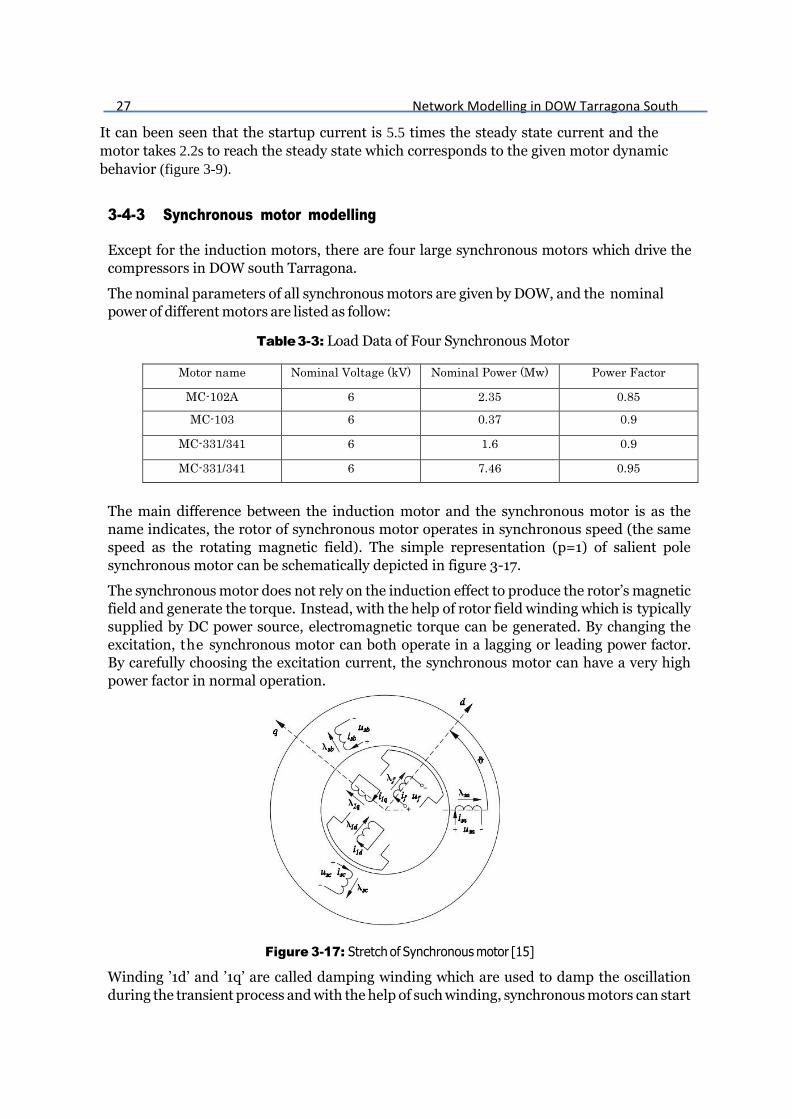
The main difference between the induction motor and the synchronous motor is as the

name indicates, the rotor of synchronous motor operates in synchronous speed (the same

speed as the rotating magnetic field). The simple representation (p=1) of salient pole

synchronous motor can be schematically depicted in figure 3-17.

The synchronous motor does not rely on the induction effect to produce the rotor’s magnetic

field and generate the torque. Instead, with the help of rotor field winding which is typically

supplied by DC power source, electromagnetic torque can be generated. By changing the

excitation, the synchronous motor can both operate in a lagging or leading power factor.

By carefully choosing the excitation current, the synchronous motor can have a very high

power factor in normal operation.

Figure 3-17: Stretch of Synchronous motor [15]

Winding ’1d’ and ’1q’ are called damping winding which are used to damp the oscillation

during the transient process and with the help of such winding, synchronous motors can start


as an induction motor (short circuit the field winding).

Compared with the induction motors, the synchronous motor has an excitation winding and therefore, the dynamic model of the synchronous motor can be described as follow (d-q frame):

1 1

1 1

0

0 0

0 0

s dd q

s qq d

f f rf

d d

q q

RU

RUd

R pUdt

R

R

(3-7)

In this thesis, we define the open circuit voltage and the motor terminal voltage as fE and

tV respectively. The angle difference between fE and tV is called the power angle which

determines the active power and reactive power consumption of the motor. Based on the

phasor diagram, the active and reacitve power consumption for salient pole motor in steady

state has been derived in the book[15]:

2| | | || |sin sin 2

2

t d qt t

d d q

V X XV EP

X X X

(3-8)

2 22

| || | sin coscos | | | |

t f

t

d q d

V EQ V

X X X

(3-9)

Typically, the load angle is quite small for large synchronous motors. By adjusting the

load angle , different active power consumption P can be obtained. The reactive power Q

can be adjusted by changing the excitation field which impacts amplitude of the open circuit

voltage fE .

Compared with the cylinder pole motors, the maximum power point angle for salient pole

(small signal stability point) is a bit lower and less than 90 degree due to the salienty. The

motor model used in this thesis is S.M 59. The input data of the synchronous motor in EMTP

is shown in figure 3-18:


Figure 3-18: Input Data in ATP-EMTP

The excitation of this synchronous motor is a simple DC excitation with under and

overexcitation regulator controlled by GTO. The DC voltage input is produced by a three-

phase full bridge diode rectifier, which is connected to the 6 kV distribution grid with a

6kV/0.38kV transformer. As the DC excitation is connected to the 6kV bus by transformers,

the voltage variation of the motor bus will impact the output of excitation. To simplify the

modelling, it can be regarded that the diode in rectifiers are ideal diodes without parasitic

capacity and the forward voltages are 0. As the excitation winding is also fed by the 25kV

feeder, both the short-circuit and open-circuit of the feeder bus affect the output of motor

excitation.

a. Opening Circuit without any Fault b.Open circuit caused by Unsymmetrical Fault

Figure 3-19: Excitation Behavior for Different Fault

As we can see in figure 3-19, a disconnecting with the power source at 1.08s contributes to a

voltage dip in the motor bus. Since the field voltage is rectified from the motor bus, the

excitation field voltage also decreases. Besides, we can see a very small voltage oscillation


which is the voltage ripple caused by the commutation of the rectifier. However, during the

unbalanced fault, the three phase input voltages are not symmetrical anymore and the

mutation of diodes lead to steep oscillations of the output DC voltage which detriments the

motor stability.

Mechanical load modelling of the synchronous motors is completely different from the

induction motor. As equation 3-7 shows, the torque curve of small rotary pumps is time

independent and the torque is only dependent with the rotation speed. However, loads of

the 4 synchronous motors are large compressors driven by a reciprocated piston.

The sketch of the mechanical structure of a simple compressor is show as follow:

Figure 3-20: The Illustration of a Compressor [17]

In order to compress the gases, the compressors have two working conditions: high load

condition and low load conditions. When the piston moves until the maximum point, the

pressure will increase gradually. If the gas pressure reaches a certain value, the discharge

valve will open to release pressure. Then the compressor goes to the low load stage which

is the opposite of the high load condition. In such a process, the pressure of the gas

decreases with an increase in gas volume. Therefore, the load curve of the compressors is an

oscillating one with maximum and minimum value, and the mechanical load of reciprocated

compressors is not only speed dependent but also time dependent. Consequently, the

mechanical load of synchronous motor cannot reach to a steady state. It is quite hard to give

an analytical solution of the reciprocated compressors since both the time and speed varies.

A widely used method is to use FEM (finite element method) to find a numerical solution.

[17]

Since DOW did not supply the torque-speed character for compressor load, this thesis

cannot model the compressor load precisely (a precise modelling requires a CFD simulation

[17] which is not the subject of this thesis). J. Wang [18] supplies a method for the qualitative

study of the compressor load based on Fourier Expansion. In this thesis, the following 4th

order Fourier series are used for rough modelling of the compressor load:

0 1 2 3 4( ) (3 ) (5 ) (7 )l r r r rT A A sin t A sin t A sin t A sin t (3-8)

The coefficients of Fourier fitting are tuned based on the stator current behavior given by

DOW, as the stator current is directly related to the motor torque. Although such load

modelling is not quite accurate when rotor speed decreases dramatically, it at least depicts

the fact that the torque would decrease with decreasing rotor speed and the reciprocated

behavior of mechanical loads in steady state.

The torque curve and current of motor MC331 are shown in figure 3-21:


a. Mechanical Load Curve b. Real-time and RMS Current

Figure 3-21: The Mechanical Load and Stator Current of Synchronous Motor MC331

As figure 3-21 indicates, the current of the motor oscillates, and no steady states can

be reached. Compared with the current recording, the coefficient of Fourier expansion can

reflect the behavior of the motor properly for normal operation. The maximum RMS

current is almost 3 times the minimum one, and therefore the input electrical power is

oscillating.

The dynamic start of the synchronous motor can be realized by a variable frequency start

with power electronic converter, but in industrial companies, the motors can start as

induction motors with the help of damper winding. There is a separate section for

synchronous startup which can be found in Appendix E.

3-6 Measurement Instruments Modelling

In order to convert the relatively high voltage and current in the power system into a safe

value for the relay operation, current and voltage transformers are applied. Typically, the

output value is range from 1-5A and 100-120V of the current transformer (CT) and voltage

transformer (VT) respectively.

3-6-1 Voltage Transformer Modelling

There are four voltage transformers used for relay testing (seen from the appendix). Two

VTs are for the feeder bus voltage measurement and two for the motor bus measurement.

All VTs are 25kV/110V with the same parameters. The equivalent circuit of VTs is shown

in figure 3-22, and all parameters are referred to the primary side.


Figure 3-22: The Equivalent Circuit of VT

In this thesis, the core saturation of the VT is ignored since the voltage during fault would

not increase too much during the fault, and the iron core is still in the linear region. All

the parameters supplied by the DOW power plant are listed in table 3-5:

Table 3-5: The Parameters of Voltage Transformer

The VT model in the EMTP is shown in figure 3-23. The VT model is composed by three single-

phase TRAFOS saturable transformers.

Figure 3-23: The EMTP Model of Voltage Transformer

3-6-2 Current Transformer Modelling

Two current transformers are used to measure the feeder bus current. All the current trans-

formers is 1600/5A with a 5P10 accuracy class. However, compared with the VT, the


saturation of the current transformer must be taken into consideration since the current

magnitude during short circuit almost 10-20 times than the nominal current, and the

magnetizing current increases, which leads to a non-linear flux behavior. It should be aware

that the secondary winding of current transformer should not be open circuit otherwise the

primary current would flow through the magnetizing loop and contributes to an extremely

high secondary voltage. The schematic diagram of CT is the same as follow:

Figure 3-24: The Equivalent Circuit of Current Transformer

The CTs in EMTP are modelled by ideal transformers with non-linear inductance NLIND96.

Based on the data given by DOW, the magnetization curve of the nonlinear inductance is

illustrated in figure 3-25.

Figure 3-25: The Non-linear Magnetizing Curve

The three-phase current transformers in EMTP are modelled based on figure 3-26. The burden

resistor lR is calculated by the rate power. 2

0.4l

rate

PR

I .


Figure 3-26: The CT Model in EMTP

3-7 Auxiliary Relay Modelling and Configuration

For the relay testing, auxiliary trip and block signals are needed. When a fault occurs in the

feeder bus, the transformer differential relay 87T and line differential relay 87 will trip the

relevant breakers in feeder bus which leads to a voltage dip. The trip signals from differential

relay should also be sent to the relay 7UV68 as an initial signal to initiate the transfer. When

a fault occurs in the motor bus, the CB in feeder bus is also tripped to cut down the power

supply by instantaneous overcurrent relay 50/50N. However, in such scenarios, the relay

7UV68 should not transfer. Therefore, the trip signal sends from overcurrent relay should

also block the fast transfer 7UV68.

Overall, two binary signals are required for the relay: initial signal from the differential relay

and block signal from the overcurrent relay. The settings of two relays should be tuned

properly to ensure that the tripping and blocking signal would not occur simultaneously.

3-7-1 Simplification for Relay Modelling

This thesis focus on the performance of fast transfer relay and the function of overcurrent and

differential relay is to send the auxiliary binary signal to the fast transfer relay. Therefore,

some simplification should be made for the differential 87T and overcurrent 50/50N relay

modelling.

General Simplification

1. Two relays have no signal resampling.

(Resampling has no impact on the relay tripping logic.)

2. The primary values are used.

(A lack of relevant measurement data, and for the normal operation the error caused by

measurement instrument can be neglect.)

Differential Relay

1. The second harmonic block function is omitted.

(We do not simulate the reclosing of unloaded transformers for 7UV68 testing and no inrush

current will flow through the differential relay. Therefore the second harmonic block is not

needed. )


3-7-2 Differential Relay Modelling

The basic principle of the differential relay is quite intuitive. Based on Kirchhoff's current law,

when a fault occurs in the protection zone, the differential current is 1 2

1 2

dif

I II C

N N

while when a fault occurs in out zone 1 2

1 2

0dif

I II

N N . Therefore the in-zone fault and out-

zone fault can be easily distinguished with very high sensitivity. However, in practice, the

differential relay should have a constraint to prevent to mal-opreation when there is a small

disturbance in the power system. Based on that a bias character of the differential relay is

designed. The minimum bias is set to be larger than the sum of the disturbance current and

possible CT errors.

Since the tertiary winding of the transformer is unloaded, the three winding transformer can

be regarded as a two winding transformer for differential protection.

In order to get the differential current and constraint current, the fundamental frequency

phasor of the primary and secondary current Ip and Is should be extracted respectively. Those

current phasors are extracted by a widely used recursive DFT (Discrete Fourier Transform)

algorithm.

First, let us consider a sinusoidal input signal with a constant frequency:

0( ) 2 ( )x t Xsin t (3-10)

This sinusoidal signal can be represented as a phasor:

( ( ) ( ))X cos jsin X

(3-11)

Assume that x(t) is sampled by N times per cycle and we have a discrete signal, the sampling

should satisfy with Nyquist Criterion to prevent a loss of information:

22 ( )kx sin k

N

(3-12)

Based on the definition of discrete Fourier transform, kx can be transformed to:

1 1

0 0

2 2 2 2( ) ( )

N N

d k k k c s

i i

X x cos k j x x sin k X jXN N N N

(3-13)

For the real-time phasor measurement, the relay works with moving window, and for a

particular window number 'w' we have:


1

1

1

2 2

2 2 2 2 ( )

4 2 ( ( ) ( )) 2

w Nw

c k

k w

w N

k w

w N

k w

X x cos kN N

Xsin k cos kN N N

ksin sin Xsin

N

(3-14)

Based on the same approach, the sine component w

sX can be represented as:

2 cosw

sX X . Hence, the DFT transformation of the signal kx can be represented as:

2( )dX Xcos Xsin and it can be proved that the DFT algorithm can extract the

phasor representation of a sinusoidal signal.

Therefore, a full cycle recursive DFT method is designed. For a digital sequence x(m) with N

values, the DFT result of window 'w+1' ( 1w

cX and 1w

sX ) is based on the value of window 'w'

( w

cX and w

sX ).

The two 230kV/25kV transformers in the feeder buses are three winding transformers with

unloaded tertiary winding. Therefore those transformers can be regarded as two winding

transformers which have a YnYn0 connection group. Such connection groups supply

convenience for relay modelling, as there is no phase shift between the primary and

secondary side. In the EMTP model is unnecessary to design the phase correction function.

Based on such RDFT method, we can obtain the current phasor in the primary side and

secondary side of the transformer during steady state and fault conditions. Consequently, we

can define the differential current and the restraining current phasors as: | |1 2

difN N

p s

I II

and1 2

0.3*| | | |N N

p s

Res

I II . When a fault occurs out of the protection zone, it is apparent

that the differential current phasor difI is almost zero and the restraining current ResI is

larger than difI . Therefore, the relay will not trip. When an in-zone fault occurs, the

differential current will be larger than constraint current and the differential relay can send

a trip signal to the relevant breakers.

3-7-3 Instantaneous Overcurrent Relay Modelling

The modelling of the overcurrent current relay is simple. The relay model calculates the RMS

value of the feeder current per phase. However, the configuration of the overcurrent relay must


take fault current contribution from motors into consideration.

The industrial motors during fault act as generators which feed the fault. Figure 3-27 indicates a

three-phase short circuit which occurs near the stator winding. During the shortcircuit

period, the motors lose a sustained power supply. In chapter 2, we derived that the rotating

magnetic field generated by field winding still exist and induce a voltage when motors lose

power supply. Driving by such voltage, there should be a current flow from the motor to the

fault point.

The settings of overcurrent relay need to be tuned properly to ensure that the lowest operating

threshold of such relay should be larger than the maximum current contribution from motors

to prevent a mal-operation when a fault occurs in feeder bus. Based on the EMTP simulation

result, the highest fault current (RMS value) contributing from motors is 3.1KA. Considering

some margin (1.2 times higher than maximuim motor current contribution), this thesis sets

the threshold of the operating current of the overcurrent relay as 3.8KA.

Figure 3-27: The Fault Current Contribution from All Motors

However, when a single phase fault occurs in the low voltage winding, the 600A ground resistor

limits the fault current at 600A. Figure 3-28.a shows that the motor will not be affected during

the fault period and operates as normal operation. Therefore, the RMS value of motor bus

current is almost the same as normal operation.

Therefore, the overcurrent relay will not trip based on the 3.8KA threshold. In order to trip the

single- phase fault, except for adding a directional component, a simple way is to detect the

zero sequence current I0, where 0 A B CI I I I . As figure 3-28.b shows, when a single

phase fault occurs in the motor bus, the level of the zero sequence current is the same as

fault current (600A). Based on that, the threshold of zero sequence current tripping is set as

500A. With a combination of instantons overcurrent relay and zero sequence current

detection, the block signal can be sent to fast transfer relay reliably when a fault occurs in the

motor bus.


a. Fault Current in Time Domain b.Zero Sequence Current

Figure 3-28: Simulation of Single Phase Fault in 25kV Motor Bus

3-8 Motor Bus Residual Voltage Tracking

As mentioned in chapter 2, both the magnitude and frequency of the residual voltages decay

after the feeder CB opens. Besides, the phase angle difference between the motor residual

voltage and the reference voltage in auxiliary feeder varies. To configure a proper setting of

fast transfer relay, it is necessary to track parameters of motor bus voltage after the feeder CB

opens.

3-8-2 Voltage Frequency Tracking

The frequency tracking method which used in this thesis is quite intuitive. In this thesis, a

method called full cycle zero crossing is used.

Figure 3-29: Illustration of Zero Crossing Method


As figure 3-29 shows, the frequency of one electrical cycle is measured by calculating the time

difference between two zero-crossing point 1T and 2T .However, since the voltage signal is

discrete, it is not possible to always have an exact ’0’ point. Therefore, for a sequence x(k) if

x(N-1) is positive and x(N) is negative, the point x(N) can be regarded as a full cycle zero

crossing point.

Figure 3-30 a shows the voltage signal after the breaker opens and 3-30 b illustrates the

frequency of the voltage signal.

a. Voltage Signal b.Instantaneous Frequency

Figure 3-30: Frequency Measurement of Voltage Signal

Compared with other frequency measurement method, zero-crossing method is easier to

implement for real-time measurement because of the extremely low computational

complexity. Besides, since this method measures a global frequency of the period 2 1mT T T

, the sharp changes and sparks would not contribute to instability of measurement. The main

drawback of zero-crossing method is such method can only measure the average frequency of

one electrical cycle which contributes to measurement inaccuracy. However, in this project,

the frequency measurement does not require high accuracy, and zero crossing method is

acceptable.

3-8-3 Voltage Amplitude and Phase angle Tracking

Typically, the amplitude of voltage signal can be measured by the RDFT (Recursive Discrete

Fourier Transformation) method as we talked in 3-6-2. However, such method is only valid

under fundamental frequency. As chapter 2 and chapter 3-7-1 shows, the frequency of

voltage in motor bus decays and RDFT method is not possible. Fortunately, in this thesis, we

only focus on the behavior of motor bus voltage after all motors lose power supply and in

such period the residual voltages are symmetrical. Therefore, the Clarke transformation

method which used for only symmetrical power system can be used.

Supposing we have symmetrical three-phase voltage signals (V 2 )a Acos t

22 ( )

3bV Acos t

and

22 ( )

3cV Acos t

, such three signals can be represented by


a rotating space vector which can be composed by two perpendicular signals V and V. To

maintain the same magnitude of voltage signals before and after the transformation, the

transformation matrix is equation 3-15:

1 112 2

2 10 13 3

1 1 102 2 2

V V

V V

VV

a

b

c

(3-15)

Based on equation 3-15 and the representation of signals aV bV and cV , we can obtain:

( )

( )

V

V

Acos t

Asin t

(3-16)

Based on 3-16, the real-time amplitude of the three phase voltages can be easily acquired as:

2 2VVA (3-17)

Besides, it can be derived that:

actaV

Vn

(3-18)

where t is the real-time phase of the signal Va . If the real-time phase angle of the motor

bus residual voltage and the reference source voltage is res andref , then the phase angle

difference between such two signals isref resd .

Figure 3-31 indicates the voltage amplitude A and delta phase angle d between the motor

bus and reference feeder bus when the breaker of faulty bus opens inadvertently.

a.Voltage Amplitude A b.Phase Angle Difference d

Figure 3-31: Voltage Amplitude and Phase Angle Difference in Open Circuit Condition

As we can see in figure 3-31， the Clarke transform method has a very fast response for system

transients. Such a method will give a clear indication of how the amplitude and phase angle

difference changes.


However, the fault cannot always be symmetrical, which leads to unsymmetrical voltages in the

three phases during the fault. As figure 3-32 shows, the double-phase-to-ground fault in high

voltage winding of the transformer leads to the unsymmetrical motor bus voltages. Therefore,

in such an unsymmetrical fault period, both the magnitude (blue line in 3-32a) and phase

difference measurement (3-32b) is unstable. When CB tripped by the differential relay, the

three phase voltages become symmetrical again and consequently, the measurement starts to

be accurate again. Since the goal of this thesis is to analyze the residual voltage after CB opens

in fault bus, the unsymmetrical period (fault period) can be ignored.

a.Voltage Amplitude b.Phase Angle Difference

Figure 3-32: Voltage Amplitude and Phase Angle Difference under unsymmetrical condition

42 Test Setup Design

Chapter 4

Testing Setup Design

4-1 Introduction

In chapter 3, the simulations are accomplished by ATP-EMTP, and both the analog and

binary signals can be obtained from the simulation. In this chapter, the setup is proposed for

the fast transfer relay testing. The overall hardware connection of the testing setup is shown

in figure 4-1:

Figure 4-1: The Overall Testing Setup

As figure 4.1 indicates, the whole testing setup is composed of 2 Omicron amplifiers (CMC356

and CMS156), a computer controlled OCC control center, and a Siemens PLC. The OCC

control center sends the fault signal recordings simulated by EMTP to Omicrons. After

testing, the control center receives and visualizes all testing results and recording. The

amplifiers are used to send the real test signals (analog and binary) to the relay and receive

the breakers’ reaction and relay binary output during testing. The PLC which shows a

significant role in the testing is programmed as three 25kV vacuum breakers for main-tie

configuration. The PLC sends the breaker states to the relay by 2-bit digital numbers, and


the position should change when the relevant command is sent by the relay. The following

parts elaborate the details of designing test setups.

4-2 Simulation Results Recording

To prepare the testing, first step is to convert the EMTP simulation result into OCC files

which can be used as the input of Omicron. Figure 4-2 is the schematic drawing of relay

input and output connection. Based on that we can see there should be ten analog signals

input for the relay operation. The line to line voltage abV(green line) and phase current

bI (blue line) of both feeder buses and three-phase motor bus voltages aV

bV and cV

(yellow line) in both side of the motor bus should be recorded. Besides, three binaries

signals (red line) inputs should also be saved to Omicron Control center to send the

initiating and blocking commands to the relay 7UV68 in the testing

Figure 4-2: Analog and Binary Signals Sending to the Relay 7UV68

As discussed in chapter 3, the vacuum breakers are controlled both by fast transfer relay

7UV68 and auxiliary relays (instantaneous overcurrent relay 50N and differential relay 87T).

Therefore, one additional binary output of Omicrons is required to simulate the trip signal

which trips the vacuum breaker in 25kV feeders by auxiliary relays.


Therefore, four binary signals and ten analog signals should be recorded by ATP-EMTP and

then converted to OCC (Omicron Control Center) files. The OCC files are created by the

following steps: First is to save the interested signals to PL4 files for different fault scenarios,

followed by converting PL4 files to COMTRADE files.

Next, a single advanced transplay test module can be made. Such a module can obtain the

test signals from both COMTRADE and DAT format. Then signal repetitions are needed to

enlarge the period of steady state signal since the operation of the relay 7UV68 requires at

least 10s steady state signal input. (Considering the calculation complexity the steady state

in the EMTP simulation is 1s).

Finally, all advanced transplay test modules for different test cases are integrated into the

OCC test library as figure 4-3 indicates. When performing a test, each embedded function in

OCC will be executed sequentially. However, in the testing for 7UV68, the breaker position

should be reset before a new test module. In this thesis, all testing modules are executed

manually instead of the automatic execution.

Figure 4-3: The OCC Test Library for Different Fault Scenarios

4-3 Test Signals Generation

Both the analog and binary signals sending to the fast transfer relay are generated by 2

Omicrons CMC356-ETH2 and CSM156. Those two Omicrons are connected by Ethernet, and

can be controlled together by the OCC computer control center via WIFI or Ethernet. The

basic technical data of 2 amplifiers are shown as follow:


Figure 4-4: Basic Technical Data of Two Amplifiers

The connections of all analog signals are intuitive. The analog output of the Omicrons is

just directly connected to the related relay terminals. However, the binary outputs of

Omicrons (binary inputs of the fast transfer relay) as we can see in figure 4-2 connect a DC

voltage output and act as a switch. Once the binary signal of Omicron output is ’1’ (high),

the switch which connects the relay with the DC voltage supply closes. Subsequently the

related terminals of the relay (block or initial) would see a 110v DC voltage, and the relevant

commands will be executed by the fast transfer relay.

Except for sending the binary signals to the relay, amplifier CMC 356 also receives the binary

signals which send from the relay 7uv68 and PLC (breaker close and open time, load shedding

time, command sequence). The input binary signals ’1’ and ’0’ (high and low) to the Omicron

correspond to the DC voltage potential difference of between the ’+’ and ’-’ . The threshold

for ’1’ are set as 77V which means if the DC voltage potential of the two ports is larger than

77V then the binary input to the Omicron is regarded as ’1’.

4-4 Breaker Time Delay Imitation

As we talked in chapter two, 25kV breakers in DOW power plant are controlled by both the

differential relay 87T and the fast transfer 7UV68. When the trip command is sent by either

differential or fast transfer relay, a DC voltage would be applied t o t h e b r e a ke r s .

T h e n , the opening coil of the breaker would induce a magnetic force which unlatches the

open spring. After that, the moving contact of the breakers separates very fast from the

stationary contact and eventually the breaker trips. On the contrary, when the closing

command is sent to the breakers, closing coils are energized, which leads to unlatch the close

spring. Then the breaker close and the charging motors charge the spring to prepare for next

closure.

However, in our testing setup design, it is unnecessary to connect the relay with 3 real breakers

which increase the overall cost of the testing. Besides, the closing and tripping of the 25kV

breakers contribute to enormous noises. Therefore, a PLC is used to imitate the breaker time

constants. Before the time delay imitation, the basic theory of breaker should be clear.


The breakers, as the name indicates are used to break current under abnormal conditions such

as short circuit. In normal conditions, the breakers which act as good conductors are in the

closed position, and the current flows from the contacts. When a release latch is energized, the

breaker cannot close or trip immediately because of the latch release delay and the moving

time of the contacts. Therefore, it should have 3 states for a breaker: close state open state and

a dynamic process between close and open called intermediate state. Besides, three constants

are defined for vacuum breakers the total breaking time, open time and close time.

As figure 4-5 shows, when a breaker receives a trip command from the relay, it needs time

for coils unlatch the springs to separate contacts of three phases. The time duration from

receiving a trip command to contact separation is called close time. After the contact

separation, there is arc ignition and the current still goes through the breaker until the arc

extinguishes; this period is called arc time. The sum of both close time and arc time is called

breaking time (tripping time). breaking close arcT T T

Figure 4-5: Time Constant of Breakers for the Breaker Opening

In contrast, when a breaker opens (figure 4-6), the close time for such breaker can be defined

as the time period after coil receives closing command until all contacts in three phases are

contacted with each other. However, the electric field of two contacts increases when the air

gap decreases. Therefore, the vacuum gap will breakdown before contacts close and the

current will flow through the breaker before contacts close.

The three breakers in DOW power plant have an average opening time about 30ms and

close time 50ms. Considering the breaker usually takes about one electrical cycle to

extinguish the arc (arc time 20ms), the total breaking time is about 50ms.


Figure 4-6: Time Constant of Breakers for the Breaker Opening

For simulating both the breaking and the opening time of the vacuum breaker, a Siemens

LOGO PLC is used. The PLC is a universal logic module integrating analog and digital

control functions as well as interface of Ethernet communication. The basic module of LOGO

PLC with display and configuration panel contains 8 digital inputs and 4 digital outputs. If

analog control functions and more digital portal are required, the PLC basics should be

extended by expansion modules. LOGO basics support a maximum of 24 digital inputs, 8

analog inputs, 20 digital outputs, and 8 analog outputs. The expansion modules connect to

the basic module by physical connection.

Table 4-1: Basic Technical Parameters of Basic Module and Expansion Module of PLC

Module Type Power Supply Input Output

LOGO! 230RCE 115 VAC/VDC to 240 VAC/VDC 8 digital 4 relays(10A)

LOGO! DM16 230R 115 VAC/VDC to 240 VAC/VDC 8 digital 8 relays(5A)

Figure 4-7 shows the connections of the PLC. The input of the PLC connects to both the

trip/close command terminals of the 7UV68 (red array) and one Omicron binary output

(purple array) which imitates the trip signal from differential relay 87T.


Figure 4-7: Connections of LOGO PLC

The outputs (digital outputs) of the PLC are simple switches between DC voltages and

"position state" indication ports of the relay. By controlling the output of PLC, the relay

will see different breaker states and based on that we can use PLC to imitate the breaker

delay.

As figure 4-7 shows, in fast transfer relay, two ports represent one particular state of a

breaker. Taking breaker CB1 as an example, a high voltage potential (110V) in terminal

CB1_52b means the breaker is closed while high voltage potential in CB1_52a indicates that

the breaker is open. If there is no voltage potential in both ports "CB1_52a" and

"CB1_52b", the relay will know that the breaker is in the intermediate state. Both ‘high’ in

those two ports are not available for the relay. If we regard high voltage potential as a digital

number ’1’ and zero voltage potential as ’0’, then a 2 bits digital number can represent a

particular position of the breaker and the truth table of breaker state as shown as below:

Table 4-2: Truth Table of Breaker State

As there are 3 breakers in the testing, 6 digital inputs and outputs are required.

The controlling and programming of the PLC can b e either realized by the control panel

in LOGO basic or by a computer which connects the LOGO PLC by Ethernet. In practice, it

is more convenient for users to control and program the PLC by a computer compared with

using the control panel. The control software used in this thesis is LOGO Soft Comfort 8.1.


Internal logic in PLC is programmed by Ladder graph, a graphical way to indicate the

relationships between input and output. Except for the basic functions which a r e given

by the software, LOGO SOFT also allows users to create new logic and control functions.

The ladder graph which is designed for the breaker simulation is shown in figure 4-8:

Figure 4-8: Ladder Diagram of PLC

In this thesis, we only focus on the main-tie configuration, so CB3 is always closed. Therefore,

in the ladder diagram output Q5 and Q6 are ’0’ and ’1’ respectively.

Usually, the lasting time of the trip and close signals are very short (about 200ms), and

the command only acts as a trigger which unlatches the closing and tripping spring of breakers

respectively.

In PLC programming, the trigger functions are accomplished by SR flip-flops as figure 4-8

indicates. SR flip-flops have two inputs R S and two output Q , Q . SR flip-flops is a

rising edge sensitivity latch, which means that the output of SR flip-flop only changes when

a single rising edge occurs. It is not available that the two inputs are in the high state. The

table below is a truth table of an SR flip-flop (the outputs state at this moment right now

have Q=Q，Q Q ).

Table 4-3: Truth table of SR Flip-flop


As mentioned before, the tripping delay and the opening delay are both about

approximately 50ms. Those delays are simulated in the LOGO by delay functions. When

simulating the vacuum breaker delay, the internal delay of PLC should be taken into

consideration. The internal delay of PLC is about 40ms. Therefore, a 10ms rising edge

sensitivity delay is added before the PLC output.

In motor bus transfer, motors are required to transfer from one feeder bus to another. Before

the feeder fault occurs, either CB1 or CB2 should be in closed state. The close state of

breakers are fulfilled by a ’wiping relay function’. Although the binary input is ’0’ at the

beginning, a combination of wiping relay block and ’or’ block (as figure 4-8 indicates) can

send a 10ms pulse with high voltage potential ’1’. Such pulse leads to a high voltage potential

output ’1’ in Q4 and low voltage output ’0’ in Q3. Consequently, relay will see a closed state

of CB2.

Before transferring the logic data to PLC, the output can be simulated in LOGO Soft. Figure

4-9 shows the simulation result of PLC ladder graph for the initial state. The blue line

indicates the low voltage potential ’0’ while red line represents the digital output ’1’. Based

on table 4-2, it is clear that CB1 is open while CB2 and CB3 are closed.

Figure 4-9: Simulation of PLC Ladder Graph

Chapter 5

Relay Testing

5-1 Introduction

All of the previous chapters are preparations of the relay testing. In chapter 3, the DOW

power plant is modelled and testing hardware is designed in chapter 4. Before testing, the

requirement should be specified. Based on different requirements the relay 7UV68 has a

different setting. In this thesis, the desired relay setting should be configured based on

having a short transfer time and small inrush current and torque when auxiliary feeder

closes. The relay is tested under the desired setting. The whole testing process has two main

parts. First, the testing should be done based on the fault locations to ensure the relay can

operate in abnormal conditions and contingencies which the DOW power system may

encounter. Next, to understand the impact of fault time and communication delay on the

transfer behaviors, a sensitivity testing should be done. Based on the sensitivity testing the

DSOs and DOW power plant will have a clear understanding of the worst scenarios and some

relevant approaches can be implemented to prevent such scenarios.

5-2 Test Requirement and Test Cases Design

5-2-1 Test Requirement

From the perspective of system engineering, the testing should be done based on the relevant

specification and requirements. Next, the test cases which acts as an input of the testing

should be designed based on the requirements.

Figure 5-1 is a sketch of the power plant in Tarragona. As figure 5-1 indicates, the fault can

occur in 230kV transmission grid, feeder buses, as well as the motor bus. For these three

types of fault locations, different requirements should be developed.

52 Relay Testing

Figure 5-1: The sketch of Tarragona power plant

Basic requirement

1. The relay 7UV68 should ensure a safe ( 1.33diff

fre

U

q PU/Hz) and fast transfer for all

abnormal and fault conditions in its protection zone.

2. Taking requirement one as a premise, the transfer time and transient torque caused

by breaker shifting should be as small as possible.

3. Before shifting the fault feeder to auxiliary bus, all synchronous motors should be

disconnected from the 25kV motor bus. During the fault and voltage dip period, the load

angle of the synchronous increases and it is impossible to track the real-time load angle by

7VU68. Besides, from the simulation and the DOW’s fault record, some synchronous motors

lose their stability after about 100ms. Considering the breaker time and fault time, for most

fault cases, the synchronous motors cannot maintain the stability before closing the auxiliary

breaker. In order to prevent the instability caused by reconnecting the synchronous motors,

the relay 7UV68 should trip such motors before bus shifting. After a successful transfer, the

synchronous motors can be manually restarted.

The specific requirements of different fault locations are listed as follow:

Feeder Bus Fault

The relay should have a breaker inadvertent open detection function.

53 Relay Testing

The elementary function of the fast transfer relay is to transfer from the fault feeder to the

auxiliary feeder. Typically, the trip signal from the differential relay would initiate the relay.

However, if the communication channel is congested or mal-operation of workers, the breaker

in the feeder bus will open without any auxiliary relay indication. Therefore, the relay should

detect the breaker opening and initiate a transfer.

Motor Bus Fault

The relay should be blocked reliably by a blocking signal.

As elaborated in chapter 3, the feeder breaker can also be tripped by motor bus over-current

relay when a fault occurs in the motor bus. In such scenarios, the relay should be blocked as

there is no fault in the feeder bus.

Fault in 230kV Transmission Grid

The relay should initiate a self-transfer which avoids a fault when a voltage dip is caused by the transmission grid fault.

The fault may also occur in 230kV transmission lines which are connected to TP or TR.

Such a grid is owned by a relevant TSO Company. The protection in transmission grid such

as line differential and distance protection will trip the relevant breaker and lead to a voltage

dip in the 25kV motor bus. In order to ensure the system stability, the fault in transmission

grid should be tripped less than a given time (critical clear time). Different TSOs has a

different grid code for the critical fault clear time. Based on the grid code from Tennet [19],

the critical fault clear time for EHV (extra high voltage) transmission grid is defined as

150ms.

Both the transmission grid fault and the feeder bus fault results in a voltage dip in the 25kV

motor bus. However for a transmission grid fault, no fault indication is sent to the fast

transfer relay. Therefore, in order to initiate a transfer to the auxiliary feeder when a fault

occurs in transmission grid, a self-start function should be designed to initiate the transfer

although no indication is sent to the fast transfer relay. However, we do not want to initiate

the transfer during the fault period, which leads to a severe stability problem, so the transfer

should be blocked during the fault period. A very simple way to prevent a transfer during a

fault is to create a blank time which is longer than the critical fault clear time for 230kV

transmission grid. The self-start transfer will be initiated after such a blank time. Based on

the grid code, the self-start function should not initiate in 150ms after a voltage dip in the

25kV bus to wait for the extinguishing of fault current.

5-2-2 Test Cases Design

The test cases are designed by requirements. After each test, the fault records from Sigra and

Omicrons are saved. The period after fault feeder trips until reference auxiliary feeder close

is called transfer time in the following chapters. Such transfer time is recorded from the fault

recording. All the testing cases are listed as follow:

Feeder Bus Fault

Faults are designed near the primary and secondary winding of both transformer TP and TR.

54 Relay Testing

Since the fault location is near the transformer winding, the transformer differential relay will

regard such fault as an in-zone fault. Therefore, the pre-designed differential relay model will

trip the relevant breakers and send the initial signal to the testing object (7UV68).The test

list for transfer from BUS1 to BUS 2 for feeder fault cases listed as table 5-1(BUS2 to BUS1

is the same):

Table 5-1: Test List for Feeder Fault

Transfer Direction Fault Location Fault Type

BUS1 to BUS1

25kV

Three-Phase

Double-Phase-to-Ground

Phase-to-Phase

Single- Phase

Inadvertently Open

230kV

Three-Phase

Double-Phase-to-Ground

Phase-to-Phase

Single- Phase

Inadvertently Open

Motor Bus Fault

Since we only test the relay under the main-tie configuration, the motor bus voltage in motor

bus 1 and 2 are the same. Therefore, only 4 testing cases are needed (single-phase, phase-

to=phase, double-phase-to-ground, three-phase).

Transmission Grid Fault

The transmission grid fault can be either a short circuit fault or open circuit fault. In the

transmission grid fault, the differential relay cannot send the initial signal. Five testing

cases are designed with four types of short circuit cases and one open circuit fault case.

5-3 Relay Configuration and Testing for Feeder Bus and Motor

Bus Fault

5-3-1 Motor Bus Residual Voltage Behavior after Fault

To configure a proper relay setting, first, the motor bus residual voltage behaviors after

breaker opens should be analyzed. For most cases, the breaker is tripped by differential or

overcurrent relay when a fault occurs. Different fault types should have different impacts

on the motor residual voltage after the fault is cleared (breaker opens). (Fault time is

designed as 70ms and communication delay are set as 20ms for all testing cases for the

relay configuration). Besides, the breaker can be opened inadvertently by mal-operation or

defection of breakers. Table 5-2 illustrates the phase angle difference d between the

motor bus voltage and reference feeders, amplitude, and frequency of the motor bus voltage

after the fault feeder trips for each fault scenarios.

55 Relay Testing

Table 5-2: Voltage Amplitude and Delta Phase Angle after Fault

At first, we can see that the inadvertent opening of the feeder breaker contributes to a

small voltage and frequency decay, although there is no short circuit fault before the breaker

opens. Moreover, there is a 27.28

phase angle shift between the motor bus voltage and the

feeder bus voltage. The reason for the amplitude and angle change can be described as

follows. Induction motors account for the majority of loads in DOW power plant. Such

induction motors operate asynchronously at the instant when the feeder breaker opens. The

amplitude, real-time phase and frequency of the induced voltage in the motor bus is

directly relevant to the motor rotation speed. Therefore, the asynchronous rotating speed

r (lower than synchronous electrical speed) leads to a changing of both voltage magnitude,

frequency and phase angle although there is no fault before the breaker open. Figure 5-2

indicates the voltage amplitude A and voltage phase difference d between the motor bus

and auxiliary feeder source.

Figure 5-2: The Voltage Magnitude, Frequency and Delta Phase Angle for Breaker Inadvertent Opening

Besides, what should attract our attention is the single-phase fault. The amplitude of motor

bus residual voltage uA and phase angle difference d for single-phase fault in the

Fault Location

Fault Type Phase Angle

Difference(degree)

Voltage Amplitude

Compared with nominal

Value (%)

Frequency

(Hz)

25kV side

Single-phase 27.76 91.31 48.91

Three-phase 79.21 47.63 47.05

Phase-to-phase 52.6 62.29 47.85

Double-phase-to-ground

52.728 61.54 47.84

230kV side

Single-phase 41.21 72.63 48.31

Three-phase 75.74 47.23 47.31

Phase-to-phase 48.12 63.91 47.89

Double-phase-to- ground

56.12 57.83 47.74

Breaker inadvertent open 27.28 91.72 48.94

56 Relay Testing

25kV feeder bus is almost the same as the inadvertent opening of the breaker. This means

that the single-phase fault in 25kV feeder bus has almost no impact on the behavior of motor bus residual voltage. With the help of 600A ground resistors in the 25kV winding, the single-phase fault current is limited at 600A, and the current flows from the feeder to

the motor bus is almost the same as normal operation. Seen from figure 5-3, the stator current and motor rotating speed during the single-phase fault is the same as normal operation. That is the main advantage of the 600A ground resistor in the 25kV winding.

a.The stator current b.The rotor speed

Figure 5-3: The Stator Current and Speed Behavior of Induction Motor during Single Phase Fault

For a single phase fault in the 230kV side, as there is no grounding resistor, one of the stator

winding loses power supply and motors supply current to the fault point which leads to a

weakening of trapped magnetic energy in the fault period. Therefore, the voltage amplitude

uA and frequency f would be lower than single-phase fault in 25kV side after breaker

opens.

Furthermore, in table 5-2, the three-phase fault leads to the highest voltage dip and phase

difference. For the three phase faulty period, except for no electrical power input, all three

phase supplies current to the fault location, which weakens the trapped magnetic energy

dramatically and therefore, leads to a maximum voltage decay and phase difference.

5-3-2 Relay Setting Configuration

Before the testing, the fast transfer relay should be configured properly. As shown in chapter

2, the safety of the transfer is ensured by the boundary threshold of each transfer modes, so it

is essential to set a proper threshold. Both the Siemens [16] and Beckwith company [20] give

a different suggested threshold setting for fast transfer mode for typical industrial companies.

However, such pre-configured thresholds may not be optimal for every power plant and

should be adjusted based on the different requirements. Before tuning the relay setting for a

different transfer mode, the synchronous motor load shedding should be added.

During both short circuit and open circuit period, the load angles of synchronous motors keep

increasing.

57 Relay Testing

As the load angle of synchronous motors is unknown, the re-energizing of synchronous

motors may lead to instability of the system. Therefore, a conservative way is to trip all

synchronous motors before auxiliary feeder closes.

The relay 7UV68 does not supply the synchronous load shedding function. Therefore, it

is necessary to add such function by CFC logic. The CFC is an integrated logic

programming tools in Digsi. Relay 7UV68 prepares the spare terminals for additional CFC

functions. It is desired that the load shedding signal is sent at the moment when the relay

sends the close signal to the auxiliary breaker. Based on such logic, the load shedding

function is designed as follow:

As figure 5-4 shows, the input signals are the close commands for both CB1 and CB2. As

such two signals connect to a ’or’ logic, a close signal of both CB1 and CB2 lead to a load

shedding and the synchronous motors can be tripped when shifting breakers.

Figure 5-4: The CFC logic of Load Shedding Function

As table 5-2 shows, at the instant the breaker in fault feeder opens, except for the case of

single-phase fault in the 25kV side, most fault cases leads to a severe voltage dip and a large delta phase angle. Therefore, for those fault case with large voltage dip and delta phase angle, it is not possible for the relay to transfer in fast mode (real-time fast mode) since the voltage angle cannot fulfill the relevant thresholds. The optimal way is to transfer such faults in the in-phase mode which can decrease the high inrush torque caused by a

large voltage difference diffU between reference feeder source and motor bus.

However, the single phase fault in the 25kV side would not contribute to large voltage dip and phase angle difference. Based on the simulation result (table 5-2), at the instant when CB1

is tripped the delta phase angle is 24.98° and the voltage amplitude is about 90% of the

nominal voltage. Therefore, it is possible for the single phase fault in 25kV bus to initiate either a fast transfer or real-time fast transfer mode based on different setting configurations.

The selection of the fast transfer mode or the real-time fast mode is based on the testing result

of transfer time and motor inrush torque. By such results, a proper transfer mode has been

chosen.

If the boundary threshold of the delta phase angle d is set as 30 , then the relay will

transfer in fast mode with a 98 ms transfer time. The fault recording and operation sequence

of the relay are shown in 5-5 and 5-6 respectively:

58 Relay Testing

Figure 5-5: Relay Operation Sequence for 25kV single phase Fault

Figure 5-6: Delta Phase Angle Recording for 25kV single phase Fault

Following the same procure with different setting (delta phase angle d is set as 20 ), the

single-phase fault in the 25kV side would initiate a real-time fast transfer mode with a

243ms transfer time. From the perspective of motor transfer time, fast transfer mode has a shorter transfer time compared with the real-time fast mode, which means the fast transfer motor has less interruption of the industrial process. However, the transfer time is only one dimension to evaluate the transfer performance. Except for the transfer time, another essential criterion to evaluate the transfer is the inrush torque when the auxiliary feeder closes. Therefore, the torque behavior should be analyzed for those two transfer modes.

By applying such transfer time in EMTP simulation, the inrush torque behavior of motors

(taking induction motor M1b as an example) when auxiliary feeder closes for two transfer

modes are shown in figure 5-7.

59 Relay Testing

a. Real-time Fast Mode b.Fast Mode

Figure 5-7: Comparison of Inrush Torque by Two Transfer Modes

As illustrated in figure 5-7, the maximum inrush torque for fast mode transfer is almost twice

as the real-time fast mode, although the transfer time for fast mode is quite short. The delta

phase angle behavior during bus transfer is shown in figure 5-8. It can be shown that the

phase angle difference in fast mode transfer is quite high (almost 90) compared with the

real-time fast transfer mode (31). Such large voltage angle difference contributes to high

inrush current and therefore, leads to a large inrush torque.

a.Real-time Fast Mode b.Fast Mode

Figure 5-8: Comparison of delta phase angle by Two Transfer Modes

Figure 5-9 shows the maximum torque behavior of all induction motors, and it can be

concluded that although the magnitude of the inrush torque of each induction motors is

different, the maximum inrush torques for all motors in fast mode are higher than real-

time fast mode for single phase fault in 25kV side .

60 Relay Testing

Figure 5-9: Maximum Inrush torque of motors for 25kV LN Fault

The reason why fast transfer mode leads to a high inrush torque compared with real-time

fast mode are elaborated as follows. As we can see in chapter 4-3, after the breaker receives

a close command, due to the delay of the magnetic coil and mechanical drag, the breaker

cannot close immediately. Such delay is called breaker closing time. During such closing

time, the motor bus is still disconnected from the power source. Therefore, the speed of all

motors keeps decreasing and leads to a large voltage amplitude and phase angle difference.

However, the fast transfer mode requires a relay reaction with a high speed. To achieve

such high-speed transfer, the computational complexity must be decreased, and there is no

prediction of the voltage amplitude and phase angle difference diffU and d . For large

power system with high overall inertia, the breaker closing time will not have too many

impacts, since the mechanical speed r of all the motors cannot drop too fast. However,

in DOW Tarragona, except for low inertia, the static loads exacerbate the decreasing of

motor speed. Thus, the difference of phase angle and voltage changes dramatically during

the breaker closing time and even leads to a 90 phase angle difference. In summary, for

the power system with low inertia, the fast transfer mode is not a good choice from the

perspective of enhancing the lifetime of motors.

Compared with the fast transfer mode, the real-time fast mode as the name indicates， can

estimate the real-time amplitude and phase angle difference caused by the breaker closing

time. The relay in real-time fast mode sends a closing signal to the breaker based on the

estimation of voltage parameters in the next 50ms instead of the instant right now.

Overall, since the 240ms transfer time is acceptable for DOW Tarragona, it is better for all

motors in 25kV single-phase fault to transfer in real-time fast mode to decrease the inrush.

61 Relay Testing

5-3-3 Relay Testing Based for Feeder or Motor Bus Fault

As the fault time and signal transmission delay would impact the transfer time and mode,

which will be illustrated in chapter 5-5 and 5-6, the testing based on fault locations and

fault types should have a constant fault time and a signal communication delay. In this case,

we suppose that both the auxiliary relays (transformer differential relay 87T) and

communication links operate in normal condition. Based on that, a typical fault time 50ms

and communication delay 20ms is used in the following testing.

The testing is to ensure that the relay can operate when contingencies occur in feeder bus

and are blocked when faults occur in the motor bus. The figure 5-10 gives an overview of the

transfer modes and transfer time (time period after fault feeder trips until auxiliary feeder

close) in different locations with different fault types. The fault locations for feeder fault

testing are designed near the 230kV and 25kV winding which is in the protection zone of the

transformer differential relay 87T. The fast transfer relays are required to have a bi-

directional transfer, so the testing results include the transfer time and modes from bus1 to

bus2 or the opposition.

For the motor bus fault, the relay should be blocked by the block signal sent from overcurrent

relay, and no transfer would be imitated when faults occur in the motor bus, which ensures

the selectivity of the relay. As illustrated in figure 5-10 and figure, no motor faults initiated a

motor transfer.

For all feeder fault cases, there is no big difference on transfer time whether the transfer is

initiated from feeder1 to feeder2 or the other way around. The time differences between two

transfer directions are less than 10ms. Such time differences are caused by the inaccuracy of

the PLC. The PLC has a ±5ms inherent operation error. Such error can be eliminated by

repeating one testing case for several times and choose the numerical average of the transfer

time, but it is unnecessary to do such averaging since the real vacuum breakers also have an

inaccuracy in both closing and opening time.

Figure 5-10: Motor Bus Transfer Time Based on Fault Type and Location

62 Relay Testing

Except for the single-phase fault, whether a fault occurs in the high voltage or in the low

voltage side of the transformers, there is a slight impact on the motor bus transfer behavior.

Such small transfer time differences are caused by the internal impedance of the transformer

TP and TR. Due to the internal transformer impedance, the current contribution from

motors are different when a fault occursin 230kV or 25kV feeder. Consequently, the voltage

behaviors of the motor bus are different after breaker trips, which leads to a small difference

in transfer time.

For a single-phase fault, as table 5-2 indicates, with the help of 600A ground resistor, the

single phase fault in the 25kv side has almost no impact on the motor residual voltage in

whole short-circuit period. Based on the configuration, the single phase fault in 25kV side

leads to a real-time fast transfer. The fault in the high voltage side leads to a high voltage

dip and phase angle difference after breaker trips, so the relay will go to in-phase mode

transfer mode with a different transfer time.

As we get the transfer time from the relay testing, the maximum inrush torque of all motors

based on different faults can be obtained. As figure 5-10 shows, the transfer time from bus 1

to bus 2 or the opposite is almost the same. Therefore, we only analyze the torque behavior

when the transfer happens from feeder 1 to feeder 2. Figure 5-11 and 5-12 shows the

maximum inrush torque of all motors when the breaker closes in the auxiliary bus.

Figure 5-11: Maximum Inrush Torque for 25kV side fault

Figure 5-12: Maximum Inrush Torque for 230kV side fault

For the same fault scenario, the magnitudes of inrush torques of all motors are different.

The induction motor group ’mPDBb’ has encountered the highest inrush torque among all

motors while motor ’m2b’ faces the lowest inrush torque. The reason why different motor

groups have different inrush torques is explained as follows. First, the parameters of each

63 Relay Testing

25kV/6kV are different, which contributes a different equivalent impedance between the

feeder bus and all motors and leads a different inrush current and torque. Besides, the air-

gap torque of the induction motors for dynamic studies is deduced by [15]

2

S S

3( )

2e R R

r

MT p i i i i

L (5-1)

Where p is the number of poles; M is the mutual inductance between the rotor and stator;

rL is the self-inductance of rotor winding; Si , Si and Ri , Ri is the stator current and

rotor current in frame respectively.

Based on equation 5-1, it is clear that the self and mutual inductances of the induction

motor also affects the inrush torque behavior. As the inductance of all motors is different,

the magnitude of inrush torque must be different.

For different fault conditions, the relative relationship of inrush torque between all motor

keeps the same. Therefore, it is reasonable to analyze the impacts of fault types on motors’

inrush torque by examining one motor instead of all motors.

Based on that, we just take motor groups ‘m1a’ as an example. In most fault cases (except

for single phase fault), there are no large differences of the inrush torque either the fault

occurs in 25kV winding or in 230kV winding, as the transfer time and transfer mode is

almost the same for such two fault locations. The motor inrush torque decreases when a

single phase fault occurs in 230kV side compared with the fault in the 25kV side. As figure

5-10 shows, the single phase fault in the 25kV winding initiates a real-time fast transfer,

while the same fault in the 230kV side leads to an in-phase transfer mode. Based on the

simulation results of inrush torque, we can deduce that although the real-time fast transfer

mode leads to a lower inrush torque than fast mode, the real-time fast transfer mode still

results in a bit higher inrush torque compared with the in-phase transfer mode. The in-phase

mode transfer can limit the delta phase angle d less than 10°compared with the 30°

delta phase angle in real-time fast mode.

5-4 Relay Configuration and Testing for Transmission Grid Fault

For transmission grid fault, there is no initial signal sending to the fast transfer relay,

although the motor bus would encounter a voltage dip. Based on the requirements in

chapter 5-2, the relay needs to initiate a self-start when a fault occurs in the transmission

grid and be blocked during the fault period.

The difficulty of configuring the transmission grid fault is that the DOW power plant does

not know the exact fault point. We do not want to initiate a self-start transfer during the fault

period. DOW does not know where the exact fault point is in the transmission grid, but the

motor acts as a generator and supplies a current to the fault point. As the relay also

measures the feeder current, the feeder current detection function can be added to detect the

current contribution from motors and block the transfer when current flows through one

of the feeder buses when a fault occurs in tranmission grid. Besides, the transmission grid

may also encounter open circuit fault. Then the DOW power plant would see a voltage dip.

With the help of self-start function, the relay can also initiate a transfer when transmission

64 Relay Testing

grid faces an open circuit fault. In order to prevent the motor bus transfer caused by a

small voltage oscillation, it is desired to set a relatively low threshold of self-start (0.8 PU

of nominal motor bus voltage, 2Hz frequency decay and the change rate of frequency: -

0.5Hz/s in the motor bus voltage). Based on the combination of those three self-start

thresholds and fault current detection functions (line dead current), we can ensure that the

fast transfer relay cannot transfer during the fault period. Figure 5-13 shows the settings

changed from the default setting.

Figure 5-13: The Changed Setting from Suggested Values for self-Start

Based on such configuration, the relay can have a blank time (time period after a fault occurs

until relay sends the pick-up signal) shown in table 5-3 for self-start in transmission grid fault.

After such a blank time, the fast transfer relay will initiate a transfer which avoids the

transfer during the fault period. The transfer time and the mode of transmission grid fault

are listed as follow:

Table 5-3 Blank Time for Transmission Grid Fault

Fault Type Self-start Blank Time (ms)

Short Circuit Fault

Single-Phase Fault 196

Double-Phase Fault 184

Phase-to-Phase Fault 181

Three-Phase Fault 171

Open Circuit Fault 174

After the blank time in table 5-3, the fast transfer relay will initiate a transfer which avoids

the transfer during fault period. The transfer time and modes of transmission grid fault are

listed as table 5-4:

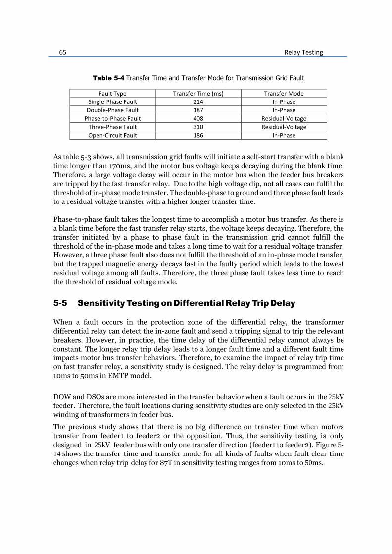
65 Relay Testing

Table 5-4 Transfer Time and Transfer Mode for Transmission Grid Fault

Fault Type Transfer Time (ms) Transfer Mode

Single-Phase Fault 214 In-Phase

Double-Phase Fault 187 In-Phase

Phase-to-Phase Fault 408 Residual-Voltage

Three-Phase Fault 310 Residual-Voltage

Open-Circuit Fault 186 In-Phase

As table 5-3 shows, all transmission grid faults will initiate a self-start transfer with a blank

time longer than 170ms, and the motor bus voltage keeps decaying during the blank time.

Therefore, a large voltage decay will occur in the motor bus when the feeder bus breakers

are tripped by the fast transfer relay. Due to the high voltage dip, not all cases can fulfil the

threshold of in-phase mode transfer. The double-phase to ground and three phase fault leads

to a residual voltage transfer with a higher longer transfer time.

Phase-to-phase fault takes the longest time to accomplish a motor bus transfer. As there is

a blank time before the fast transfer relay starts, the voltage keeps decaying. Therefore, the

transfer initiated by a phase to phase fault in the transmission grid cannot fulfill the

threshold of the in-phase mode and takes a long time to wait for a residual voltage transfer.

However, a three phase fault also does not fulfill the threshold of an in-phase mode transfer,

but the trapped magnetic energy decays fast in the faulty period which leads to the lowest

residual voltage among all faults. Therefore, the three phase fault takes less time to reach

the threshold of residual voltage mode.

5-5 Sensitivity Testing on Differential Relay Trip Delay

When a fault occurs in the protection zone of the differential relay, the transformer

differential relay can detect the in-zone fault and send a tripping signal to trip the relevant

breakers. However, in practice, the time delay of the differential relay cannot always be

constant. The longer relay trip delay leads to a longer fault time and a different fault time

impacts motor bus transfer behaviors. Therefore, to examine the impact of relay trip time

on fast transfer relay, a sensitivity study is designed. The relay delay is programmed from

10ms to 50ms in EMTP model.

DOW and DSOs are more interested in the transfer behavior when a fault occurs in the 25kV

feeder. Therefore, the fault locations during sensitivity studies are only selected in the 25kV

winding of transformers in feeder bus.

The previous study shows that there is no big difference on transfer time when motors

transfer from feeder1 to feeder2 or the opposition. Thus, the sensitivity testing is only

designed in 25kV feeder bus with only one transfer direction (feeder1 to feeder2). Figure 5-

14 shows the transfer time and transfer mode for all kinds of faults when fault clear time

changes when relay trip delay for 87T in sensitivity testing ranges from 10ms to 50ms.

66 Relay Testing

Figure 5-14: Sensitivity Study of Relay Trip Time

When a relay trip delay changes from 10ms to 50ms, the transfer time initiated by a three-

phase fault changes dramatically from a minimum transfer time 184ms (in-phase mode) to a

maximum transfer time 591ms (residual transfer mode). When the relay trip delay is

relatively small (less than 30ms), the fast transfer relay is transferred in the in-phase mode

for most fault cases (except for single phase fault). Besides, the transfer time for all fault

scenarios increases except for single phase fault with the increase of 87T trip delay.

For single phase faults, the trip delay of 87T has no impact on the transfer time. The ground

resistor in t h e low voltage side limits the fault current, and all motors in DOW power

plant operates normally. Therefore, no matter how long the single-phase fault lasts, the

motors cannot be affected during the fault period. Consequently, the motor bus residual

voltage cannot be affected although single-phase fault time changes. That is the reason why

the relay trip delay has no impacts on the motor bus transfer time.

For a phase-to-phase fault and a double-phase-to-ground fault, the dynamic behavior of

the motor bus voltage can be impacted by different fault time. A long fault time leads to

a low voltage amplitude and frequency.

During the period of three-phase fault, all three phases of the motors are lost power supply

and motors contributes to a relatively high fault current level to the fault point. Based on

the law of conservative of energy, the trapped magnetic energy depletes very fast and leads

to a relatively low voltage amplitude which is lower than the threshold of in-phase mode

after breaker opens.

As the voltage amplitude threshold UA for a residual voltage mode transfer is set at a

relatively low value, the relay needs time to wait for a residual mode transfer, which means

the amplitude of the motor bus should be lower than 0.25PU (suggested threshold are given

by Siemens [16] and Beckwith [20]). That is the reason why the 50ms trip delay leads to a

shorter transfer time than 40ms for three-phase faults. The 50ms 87T trip delay results in a

higher voltage dip than 40ms delay and therefore, takes less time to reach the 0.25PU threshold

to have a residual-voltage transfer.

Then, the inrush torque can be obtained based on the same method in chapter 5-4-1. As the

67 Relay Testing

relative relationships of the inrush torque for different motors keep the same, the motor group ‘m1a’ is chosen for the inrush torque study.

Figure 5-15: Sensitivity Study (Inrush Torque) of Relay Trip Time

As figure 5-15 indicates, except for a three-phase fault, the relay trip delay (less than 50ms)

has almost no impact on the inrush torque behavior because such fault cases initiate the

same transfer modes (in-phase transfer mode).

However, we can see a sharp increase in the inrush torque when the 87T trip delay is larger

than 30ms for a three-phase fault. In figure 5-15, it can be seen that the motor bus is

transferred in the residual voltage mode if the trip delay is larger than 30ms. Compared

with the in-phase transfer mode, there is a high inrush torque in the residual voltage mode

due to a long transfer time. A long transfer time leads to a low voltage amplitude of the

motor bus voltage and contributes to a high voltage difference between the feeder bus and

the motor bus compared with the in-phase transfer mode. Therefore, such high voltage

difference leads to a large inrush torque. In practice, the operators should take measures to

avoid a residual voltage mode transfer.

5-6 Sensitivity Testing on Communication Delay

The trip signal of 87T acts as an initial signal to pick up the fast transfer relay. However, the

differential relay is always installed very far away from the fast transfer relay and therefore,

the trip signal must be sent via the communication channel (optical fiber). Consequently, it

needs time for fast transfer relay 7UV68 to receive such an initial signal. Typically, the

communication delay takes 20ms, but in practice, it is inevitable for a communication

network to encounter congestions which increase the communication delay. For some

particular cases, such as broken communication links or routers, the fast transfer will not

receive the initial signal although the relative breaker is tripped by the 87T. The relay is still

required to transfer in such cases. The transfer is ensured by the breaker inadvertent opening

detection if no trip command is received by the fast transfer. Once the relay detects the

opening of the healthy breaker, the transfer will be initiated after a 50ms time delay.

The sensitivity testing for communication delay is also only designed for fault in the 25kV

68 Relay Testing

bus, and only one direction transfer is considered (feeder1 to feeder2). In the sensitivity

testing, the communication time is ranged from 10ms to 70ms. Besides, a special scenario

where the fast transfer relay cannot receive is also added into the sensitivity testing.

Figure 5-16: Sensitivity Study of Communication Delay

As figure 5-16 shows, the transfer time and the transfer mode will not be affected when the

communication delay is less than the breaker breaking time (50ms) because the relay has

already received the initiation signal before fault feeder opens.

However, if the communication time is longer than breaking time (60ms and 70ms cases),

there would be a blank time period that the breaker opens, but no tripping signal is received

by the relay. The longer the communication delay is, the longer the blank time will be.

During such blank time, the motor bus residual voltage resU keeps decaying and leads to a

longer transfer time for long communication delay, especially for three-phase fault. For

fault cases where the communication delay is less than 70ms, the real-time fast mode

transfer is initiated by a single phase fault, and other fault leads to in-phase mode transfer.

Besides, this thesis also considers the most severe cases where no initial signals are received

by the fast transfer relay, the bus transfer needs a long time because the relay regards the

faults without tripping signal as an inadvertent breaker opening. It needs time for the

breaker-opening-detection function to initiate the transfer. Such time delay results in an in-

phase mode transfer for a single phase fault and the transfer mode for other fault scenarios

do not change (still in in-phase modes).

Based on the transfer time of the sensitivity study, the inrush torque behaviors of motors

can be analyzed. Figure 5-17 shows the inrush torque of motor group ‘m1a’when

communication delay ranges from 10ms to infinite (no tripping signal).

69 Relay Testing

Figure 5-17: Sensitivity Study (Inrush Torque) of Communication Delay

As figure 5-17 shows, there are no big differences for the inrush torques when the

communication delay varies from 10ms to 70ms. The small torque variation is caused by the

slight differences in transfer time. However, if the fast transfer relay cannot receive the trip

signal, except for a single phase fault, other fault types lead to a higher inrush torque. For

such fault scenarios, the transfer modes do not change, but the transfer takes a long time

(more than 300ms). As we can see in chapter 5-5, a long transfer time will lead to a high

inrush torque. That’s the reason why we can see an increase in the inrush torque when no

trip is sent to the relay.

Nevertheless, for the single-phase fault cases without tripping signal, the transient torque

decreases a bit compared with the normal communication delay. Such decrease is caused

by the changing of the transfer mode (from real-time fast mode to in-phase mode). In

chapter 5-3, we can see that the in-phase transfer mode has less inrush torque compared

with the real-time fast mode.

Chapter 6

Conclusion and Future Work

6-1 Conclusion

Although some testing has been already designed to examine the transfer behavior of fast

transfer relay by engineers from industries, that testing is general testing, and no testing is

designed based on the actual power system model. Besides, no testing results have been

proposed about the motor inrush torque behavior. This thesis deals with testing of the fast

transfer relay 7UV68 based on the EMTP modelling of DOW Tarragona. Except for fast

transfer relay testing, such a power plant model can also be used for stability analysis and

configuration of other types of relays. Based on the EMTP simulation and the relay testing

result, overall conclusions are given as follows:

1. The power loss in the motor bus with running motors leads to a residual voltage resU

with a decaying magnitude and frequency in the motor bus. The reclosing of the auxiliary

feeder bus leads to a high inrush current and a torque due to the voltage parameter

difference between the reference feeder and the motor bus.

2. Sequential transfer scheme has the longest transfer time, but such scheme absolutely

avoids the motor bus transfer and the parallel operation of the two sources during the

fault period and increase the stability of the system.

3. Transfer in fast (real-time fast) mode will only happen with a single-phase to ground

faults in the 25kV feeder in DOW Tarragona plant. Other fault scenarios in such plant

will lead to transfers in in-phase or residual voltage transfer modes.

4. From the perspective of decreasing inrush torque, a fast transfer mode is not suitable for

a power system with low inertia, because such mode cannot make an estimation on the

voltage change caused by the breaker close delay.

5. The trip delay of the differential relay (87T) affects the behavior of the motor bus transfer.

A three phase fault with a long 87T trip delay is the most severe case for a relay to

transfer, as such faults contribute to the longest transfer time and the highest inrush

torque.

71 Conclusion and Future Work

6. A Short communication delay between the fast transfer relay and the

transformer differential relay (87T) has no impact on the transfer behavior of the

motor bus whilst a long communication delay (longer than breaker breaking

time) will lead to a long transfer time.

6-2 Future Work

1. Testing of the relay can be designed by a hardware-in-the-loop testing system

with RTDS (real-time digital power system simulator). With the help of real-time

simulation, it is much easier to have a comprehensive understanding of the

dynamic behavior of the motors and the impact of different faults on the

performance of the fast transfer relay. There will be two stages of designing the

hardware-in-the-loop testing. The first step is the same as this thesis, which is

the power system modelling. The second step is to design the testing hardware.

The analog signals to the fast relay will be generated from the RSCAD simulation

via Gigabit Transceiver Analogue Output (GTAO) cards and amplifiers to the

relay. The binary inputs and outputs should connect to Gigabit Transceiver Front

Panel Interface (GTFPI) cards.

2. The vacuum breakers of the 25kV bus may experience overvoltages after they are

switched off. The transient recovery voltage behavior can be analyzed by

designing suitable vacuum breakers and arc models in EMTP.

Appendix A

Testing Setup and Installation

1 Figure of Testing Setup

Figure Appendix A.1 Testing Setup and Connection

Appendix B

System Data of DOW Tarragona

1. Cable Data

Table Appendix B.1 Cable Data

Cable type Nominal/Maximu

m Voltage(kV)

AC Resistance

90C (Ω/km)

Reactance

50Hz (Ω/km)

Feeding cable

bus3:3**240 sqmm

XLPE CU 500m(BusA

and B)

18/30 0.0976 0.117

Feeding cable bus2:3*240

sqmm XLPE AL 990m

BusA 360m BusB

18/30 01.61 0.117

Feeding cable PDB:3*240

sqmm XLPE CU 360m

(BusA and B)

18/30 0.0976 0.117

Feeding cable TR-

MC:3*240 sqmm XLPE

CU 60m

18/30 0.0976 0.117

Feeding cable

principle:3*240 sqmm

XLPE CU 30m (BusA and

B)

18/30 0.0976 0.117

Cable TP to TR:3*3*1 630

sqmm XLPE AL 600

(BusA and B)

19/33(36) 0.063 0.102

Cable 230kV gird:3*1*630

sqmm XLPE CU 800m

(BusA and B)

3.8/6.6(7.2) 0.063 0.11

Appendix B

2. Load Data

Table Appendix B.2 Load Data

Appendix C

Model for Auxiliary Relay and

Additional Measurement

1 Differential Relay Model

MODEL Simple Differential Relay Model

DATA

FREQ dflt:50 -- Frequency of the first harmonic

SampleFreq dflt:400

Scale dflt:1

Algorithm dflt:1 --DFT recursive

INPUT

xt[1..3]

xm[1..3] -- The input signal which is to be analyzed

OUTPUT

--re[1..3] -- Magnitude values of the fundamental frequency component.

Phase ABC

--im[1..3]

irest[1..3]

isum[1..3] -- Magnitude values of the fundamental frequency component.

Phase ABC

trip2

VAR

re[1..3], im[1..3],OMEGA,NSAMPL,alpha,D,i,delta_T[0..7],

x7,x72,xre,xim,x[1..3],ab[1..3],ab2[1..3],re2[1..3],im2[1..3],D2,xm7,n,trip

1

irest[1..3],isum[1..3],

trip[1..3],flag,trip2,isum1[1..3]

TIMESTEP min:recip(SampleFreq)

DELAY CELLS (X[1..3]): recip(FREQ*timestep)+2

DELAY CELLS (XM[1..3]): recip(FREQ*timestep)+2 -- Need at least one first

harmonic periode of sampling

HISTORY X[1..3] DFLT:0

xm[1..3]DFLT:0 -- Fills the signal with zeroes when time <= 0

trip1dflt:0

INIT

FOR i:= 0 TO 7 DO

delta_T[i] := i/(FREQ*8)

ENDFOR

Appendix C

alpha:=1/sqrt(2)

OMEGA:=2*PI*FREQ

NSAMPL:=recip(FREQ*timestep)

if abs(NSAMPL-trunc(NSAMPL))>1e-9 then

write('%%%WARNING in ABC2PHR2: SAMPLEFREQ/FREQ is not an integer

number')

endif

re[1..3] :=0

im[1..3] :=0

re2[1..3] :=0

im2[1..3] :=0

trip[1..3]:=0

trip1:=0

flag:=0

ENDINIT

EXEC

for i:=1 to 3 do

x[i]:=8.702*xt[i]

if Algorithm =1 then

--DFT recursive moving window

x7:=delay(X[i],1/FREQ,2)

x72:=delay(XM[i],1/FREQ,2)

D:=2/NSAMPL*(X[i]-x7)*cos(OMEGA*T) --recursive DFT

re[i]:=re[i]+D*Scale

D:=2/NSAMPL*(X[i]-x7)*sin(OMEGA*T)

im[i]:=im[i]-D*Scale

xm7:=delay(XM[i],1/FREQ,2)

D2:=2/NSAMPL*(XM[i]-x72)*cos(OMEGA*T)

re2[i]:=re2[i]+D2*Scale

D2:=2/NSAMPL*(XM[i]-x72)*sin(OMEGA*T)

im2[i]:=im2[i]-D2*Scale

endif

ab[i]:=sqrt(re[i]**2+im[i]**2)

ab2[i]:=sqrt(re2[i]**2+im2[i]**2)

endfor

if flag=0 then

for n:=1 to 3 do

isum1[n]:=sqrt((re[n]+re2[n])**2+(im[n]+im2[n])**2)

if isum1[n]<20 then

isum[n]:=0

endif

irest[n]:=1/2*(sqrt(re[n]*re[n]+im[n]*im[n])+sqrt(re2[n]*re2[n]+im2[n]*im2[

n]))

Appendix C

isum[n]:=sqrt((re[n]-re2[n])**2+(im[n]-im2[n])**2)

if t>1.06 then

isum[n]:=0

endif

if isum[n]>0.3*irest[n] then

trip[n]:=1

flag:=1

endif

endfor

else

trip[1..3]:=1

endif

trip1:=or(trip[1],trip[2],trip[3])

trip2:=delay(trip1,0.02,1)

ENDEXEC

ENDMODEL

Appendix C

2 Overcurrent Relay Model

MODEL currentrelay1

DATA

freq -- base frequency

xrms_ini dflt:-1 -- initial rms value

scale dflt:1 --multiply output by this number

SampleFreq

INPUT

x[1..3] -- monitored signal

--block

OUTPUT

trip[1..3]

trip1 -- rms value of monitored signal

i0rms

VAR

xrms[1..3]

x2[1..3] -- internal, x*x

ix2[1..3]

ix20

period -- 1/freq

n

trip[1..3]

trip2

flag

trip1

i0

i0rms

x20

trip0

History

trip2 dflt:0

ix2[1..3]dflt:0

init

trip[1..3]:=0

trip2:=0

flag:=0

trip0:=0

endinit

TIMESTEP min:recip(SampleFreq) --this restricts local timestep to avoid

overflow

DELAY CELLS(ix2[1..3],ix20,trip2,trip1,trip0): 2*recip(freq*timestep)

INIT

Appendix C

period:= recip(freq)

histdef(ix2[1..3]) := 0

histdef(ix20) := 0

histdef(trip2):=0

integral(x2[1..3]) := 0

integral(x20):=0

flag:=0

IF xrms_ini <0 THEN xrms[1..3]:=0 ELSE xrms[1..3]:=xrms_ini ENDIF

ENDINIT

EXEC

i0:=x[1]+x[2]+x[3] –zero sequence current

x20:=i0*i0

ix20:=integral(x20)

i0rms:= sqrt((ix20 - delay(ix20, period))*freq)*scale–RMS value

if flag=0 then

FOR n:=1 TO 3 DO

x2[n] := x[n]*x[n]

ix2[n] := integral(x2[n])

IF t>period THEN

xrms[n] := sqrt((ix2[n] - delay(ix2[n], period))*freq)*scale

else

xrms[n]:=0

ENDIF

if (xrms[n]>6000) then

trip[n]:=1

flag:=1

else

trip[n]:=0

endif

ENDFOR

else

trip[1..3]:=1

endif

if (i0rms>500) then –threshold of zero current sequence measurement

trip0:=1

flag:=1

else

trip0:=0

endif

trip2:=or(trip[1],trip[2],trip[3],trip0)

trip1:=delay(trip2,0.015)

ENDEXEC

ENDMODEL

Appendix C

3 Frequency Measurement

MODEL fremea

DATA f0 -- initial frequency

band -- max acceptable change

INPUT x -- monitored signal

VAR f -- measured frequency

txing -- time of last detected zero-crossing

xprev -- previous value of signal

dtmin -- minimum sampling half-period

dtmax -- maximum sampling half-period

a -- temp variable

OUTPUT f

INIT

f := f0

txing := -2

xprev := x

dtmax := 1/(1-band/100)/f0

dtmin := 1/(1+band/100)/f0

ENDINIT

EXEC

IF txing = -2 THEN txing := -1

ELSIF txing = -1 AND xprev*x <=0 AND xprev<x THEN txing:=t

ELSIF xprev*x <=0 AND xprev<x AND t-txing >= dtmin AND t-txing <= dtmax

THEN – Finding Zero Crossing Point

a := backtime(x,0,1)

f := 1/(a-txing)

txing := a

ENDIF

xprev := x

ENDEXEC

ENDMODEL

Appendix C

4 Amplitude and Phase measurement

MODEL phasormeasure

INPUT u[1..3] -- phase voltages

OUTPUT vamp, ure, uim ,angle,freq

---DATA

--sample DFLT:0.0 -- phase betw. d-axis and alpha-axis

VAR

ualpha,ubeta,angle,vamp,ure,uim,vampt,freq

history

angledflt:0.00

EXEC

-- From three-phase to alfa-beta-zero

ualpha := 2/3*(u[1] - 0.5*(u[2]+u[3]))

ubeta := 1/(SQRT(3))*(u[2] - u[3]) – Clarke Transformation

vampt := SQRT(ualpha*ualpha+ubeta*ubeta)

vamp := vampt

angle := atan(ualpha/ubeta)/(2*3.141596)*360

ure := ualpha

uim := ubeta

if uim >=0 then angle:= acos(ure/vampt)

else

angle:= -acos(ure/vampt)

endif

ENDEXEC

ENDMODEL

Appendix D

The relay setting of 7UV68

1 Power System Setting for Fast Transfer Relay

Figure Appendix D.1 Basic Power System Data

Appendix D

Figure Appendix D.2 Relay Startup

Figure Appendix D.3 VT Setting

Appendix D

Figure Appendix D.4 CT Setting

Figure Appendix D.5 Minimum CB Duration Setting

Appendix D

2 HSBT (high speed bus transfer) Function Setting

Figure Appendix D.6 Overall Setting Group

Figure Appendix D.7 Setting of Transfer Initialization Function (A)

Appendix D

Figure Appendix D.8 Setting of Transfer Initialization Function (B)

Figure Appendix D.9 Transfer Sequence and Self-start Function Design (A)

Appendix D

Figure Appendix D.10 Transfer Sequence and Self-start Function Design (B)

Figure Appendix D.11 Transfer Mode Selection

Appendix D

Figure Appendix D.12 Transfer threshold of Different Transfer Mode (A)

Figure Appendix D.13 Transfer threshold of Different Transfer Mode (B)

Appendix D

3 Supervisory Function Setting

Figure Appendix D.13 Additional Supervisory Function

Appendix E

EMTP Modelling For Starting a

Synchronous Motor

This part is not relevant to this thesis. Such model is used as a reference for DOW to

simulate the motor start for Tarragona and other power plant.

Except for the startup of synchronous motor by varying frequency, which uses power electronic

converters, a simpler way can be used for starting such motors.

The synchronous machines can be directly connected to AC voltage power source. As figure 3-17

shows the synchronous motors have excitation winding and damper windings which damps the

oscillations. Such short-circuited windings act as the rotor winding of the induction motors and

with the help of such windings, the synchronous motor can start as an induction motor. As the

speed increases to the asynchronous speed, the excitation of the motor is added. With the help

of the excitation field, the synchronous motors can run in a synchronous speed.

To simulate the startup, all parameters of the EMTP model S.M.59 should be tuned precisely.

The initial machine speed should be set as a very low value (1%- 2% the nominal speed). Besides,

the initial voltage, the frequency and the capacity in the relevant synchronous motor model

should be 2% of the nominal value. When the motor speed reach 98%, the excitation field can be

added.

The synchronous motor used in this thesis is a 28 poles motor with a 6kV nominal voltage and a

9.6 MW nominal power. The nominal speed of the motor can be calculated as:

60214.28

fn

p (1)

The mechanical load used in this chapter is the reciprocated industrial load (seen from chapter

3-4), such load is added when synchronous motor reach to the nominal speed (after 5s). The

input data of the startup simulation are shown in figure Appendix E.1

Appendix E

Appendix E.1 input data of the startup simulation

As we can see from figure appendix E.2, the motor can reach to the synchronous speed at about 2s and at such period the excitation is added.

Appendix E.2 The startup of Synchronous Motor

Appendix F

Basic Testing for Simultaneous

Transfer Sequence

Such transfer sequence is not used in the relay testing in this thesis. As discussed in chapter

2, in simultaneous transfer scheme, a trip command is sent to the breaker in the faulty feeder

at the same time when the close command is sent to the switch of the auxiliary bus.

As the figure indicates, the feeder breaker is already tripped by the differential relay when a

short circuit occurs. Based on the internal logic of the simultaneous scheme, the relay sent

both the trip command to fault breaker (although such breaker has already received the trip

signal) and the close command to the healthy feeder. If the fault clearing time is longer than

the breaker closing time, the breaker in the auxiliary bus will close although the fault does not

clear. The auxiliary feeder continues to feed the fault, which makes more difficult for the fault

to be cleared and this leads to instability of the whole power system. That is the reason why

simultaneous schemes are not used in this thesis.

Figure Appendix F.1 Simultaneous Transfer for 150ms Three-phase Fault

Appendix F

However, the simultaneous transfer sequence has some drawbacks, as some basic testing for

such transfer scheme as a reference for DOW has been done. The test is only performed for

the feeder bus with 50ms breaker closing and opening time, 20ms communication delay, and

20ms 87T trip delay.

The testing result are shown as table Appendix F.1:

Table Appendix F.1

From the testing result, it is clear that the fault time has only impact on the transfer time

when the simultaneous transfer scheme is chosen. Since the close command is sent to the

auxiliary breakers at the same time when the trip command is sent to breaker in the faulty

feeder.

Fault Location Fault Type Transer Time (ms)

Single-Phase Fault 41.2

Double-Phase Fault 42.3

Phase to Phase Fault 45.7

Three Phase Fault 40.3

Single-Phase Fault 43.7

Double-Phase Fault 42.1

Phase to Phase Fault 36.7

Three Phase Fault 40.1

25kV Side

220kV Side

Bibliography

[1] F. I. Khan and S. Abbasi, “Techniques and methodologies for risk analysis in chemical

process industries,” Journal of Loss Prevention in the Process Industries, vol. 11, no. 4,

pp. 261 – 277, 1998.

[2] D. G. Lewis and W. D. Marsh, “Transfer of steam-electric generating-station auxiliary

busses [includes discussion],” Transactions of the American Institute of Electrical Engi- neers. Part III: Power Apparatus and Systems, vol. 74, Jan 1955.

[3] W. C. Huening, “Calculating short-circuit currents with contributions from induction

motors,” IEEE Transactions on Industry Applications, vol. IA-18, pp. 85–92, March

1982.

[4] K. E. Yeager, “Bus transfer of multiple induction motor loads in a 400 megawatt fossil

power plant,” IEEE Transactions on Energy Conversion, vol. 3, pp. 451–457, Sep 1988.

[5] T. R. Beckwith and W. G. Hartmann, “Motor bus transfer: considerations amp; meth-

ods,” in IEEE Systems Technical Conference on Industrial and Commercial Power 2005., pp. 62–76, May 2005.

[6] M. V. V. S. Yalla, “Design of a high-speed motor bus transfer system,” in Conference

Record 2009 IEEE Industrial Commercial Power Systems Technical Conference, pp. 1– 12, May 2009.

[7] L. Asnin, V. Backmutsky, M. Gankin, J. Blashka, and M. Sedlachek, “Dsp methods for

dynamic estimation of frequency and magnitude parameters in power system transients,” in 2001 IEEE Porto Power Tech Proceedings (Cat. No.01EX502), vol. 4, pp. 6 pp. vol.4–,

2001.

[8] M. M. Begovic, P. M. Djuric, S. Dunlap, and A. G. Phadke, “Frequency tracking in power

networks in the presence of harmonics,” IEEE Transactions on Power Delivery, vol. 8, pp. 480–486, Apr 1993.

Master thesis Wenbin Wu

95

Bibliography

[9] E. Aboutanios, “An adaptive clarke transform based estimator for the frequency of bal- anced and unbalanced three-phase power systems,” in 2017 25th European Signal Pro- cessing Conference (EUSIPCO), pp. 1001–1005, Aug 2017.

[10] V. Eckhardt, P. Hippe, and G. Hosemann, “Dynamic measuring of frequency and frequency oscillations in multiphase power systems,” IEEE Transactions on Power Delivery,

vol. 4, pp. 95–102, Jan 1989.

[11] J.-Z. Yang and C.-W. Liu, “A precise calculation of power system frequency,” IEEE Transactions on Power Delivery, vol. 16, pp. 361–366, Jul 2001.

[12] T. Lobos and J. Rezmer, “Real-time determination of power system frequency,” IEEE Transactions on Instrumentation and Measurement, vol. 46, pp. 877–881, Aug 1997.

[13] “C50.41-2000,” American National Standard for Polyphase Induction Motors for Power Generating Stations, 2000.

[14] T. R. Beckwith and C. J. Mozina, “Motor bus transfer system performance testing and

the search for a new transfer success criterion,” IEEE Transactions on Industry Appli- cations, vol. 53, pp. 653–659, Jan 2017.

[15] M. Hoeijmakers, Modelling of ac machines. Delft University of Technology, 2004.

[16] Siemens AG, Multi-function High Speed Motor Bus Transfer 7VU683, 2016.

[17] D. Homa and W. WrÃşblewski, “Modelling of flow with cavitation in centrifugal pump,”

Journal of Physics: Conference Series, vol. 530, no. 1, p. 012032, 2014.

[18] J. Wang, Z. Bao and D. Chen, “Frequency spectrum analysis of vibration signals and

fault diagnosis of reciprocating compressor,” Applied Mechanics and Material, Vols.

336-338, pp 982-987, 2008

[19] Tennet TSO GmbH, Grid Code for high and extra high voltage, 2015.

[20] Beckwith Electric Co., Digital Motor Bus Transfer System, 2004.

Date post:	05-Dec-2021
Category:	Documents
Upload:	others
View:	1 times
Download:	0 times

Masters Thesis: Testing of fast transfer relay by an EMTP ...

Documents