34
| Date post: | 08-Dec-2015 |
| Category: |
Documents |
| Upload: | haziq718507637 |
| View: | 16 times |
| Download: | 0 times |


CONTENTS
I VECTORS 3
II MATRICES 6
III PLOTS 10
IV \VORKSPACE 18
V M-FILES AND FUNCTIONS 21
VI MISCELLANEOUS FUNCTIONS 26
VII SIGNAL PROCESSING 31

~······
Kl;
3
I. VECTORS
When you run MATLAB, command window appears. All commands are written on that com
mand line. We first begin with entering vectors and basic vector operations. Let's first define a row vector whose elements are (2,4,5).
»a=[2 4 5]
a=
2 4 5
You can also put commas between the elements, there will be no difference.
»a=[2,4,5]
a=
2 4 5
Now let's define a column vector, in order to define a column vector you have to put a semicolon between the elements.
»b=[2;3;5]
b=
2
3
5
After defining a vector you may need to know what is the i'h element of the vector. For example the 3rd element of the vector b is:
»b(3)
ans=
5
Below the characters of some vector'£bpe~ations are given.
+ addition
subtraction
* multiplicatian
/ division
transpose
Multiply a and b,
»a*b
ans=
41
...... -------------------

4
c = bT, c is b transpose,
~c=b'
c =
2 3 5
add aand c,
~a+c
ans=
4 7 10 . Additionally, there are many MATLAB functions which do different operations. Some vector func
tions are explained.
CROSS: Cross product of two vectors.
~cross(a,c)
ans=
5 0 -2
DOT: Dot product of two vectors.
~dot(a,c)
ans=
41
SUM: Sum of the vector elements.
~sum(a)
ans=
11
LENGTH: Length of the vector.
~length(a)
ans = 3
However, most of. the vectors we define have length of hundreds which is not efficient to enter
all the elements one by one. There are efficient ways to do it. The following example defines a
vector whose first element is -5, last element is 2 and the subsequent elements are increasing by 1.

»d=[-5:2]
d=
-5 -4 -3 -2
5
-1 0 1 2
The default increment is 1, but you can define it as another value as in the following example,
the increment between the elements is 0.4.
»d=[3:0.4:5]
d=
3.0000 3.4000 3.8000 4.2000 4.6000 50000 J Another very important syntax is semicolon. If we use semicolon after ·the command line, the
elements are not displayed, but they are assigned. This will be useful when you do not want to see
the contents of the vector, especially when their length is large. In the following example when we
put semicolon after the command line we will not see again the elements of z, however when you want to see the elements of z just type z.
»z=[l 2 6];
z=
1 2 6

6
II. MATRICES
The general rules for defining matrices is:
»a.==[5 6 2;0 -1 -8;1 0 -2]
a=
5 6 2
0 -1 -8
1 0 -2
We use [ J for identifying matrices; we use space or comma (,) for every term of the rows and
we use semicolon for idel\tifying the columns.
To see the ij'h element of the matrix:
»a(2,3)
ans=
-8
To see the ith row of the matrix:
»a(3,:)
ans=
1 0 -2
To see the j'h column of the matrix:
»a(:,2)
ans=
6
-1
0
Let's look at some matrix functions.
SIZE: Size of a matrix.
» size(a)
ans=
3 3
matrix a is 3x3

/ "~-
INV:· Finds inverse of a matrix.
» inv(a)
ans=
-0.0556 -0.3333 1.2778
0.2222 0.3333 -1.1111
-0.0278 -0.1667 0.1389
DET: Finds the determinant of a matrix.
»det(a)
ans=
-36
EIG: Finds eigenvalues of a matrix.
» eig(a)
ans=
3.0000 + O.OOOOi
3.0000 - O.OOOOi
-4.0000
EYE: Gives the identity matrix, eye(N) is the N-by-N identity matrix.
» eye(3)
nns =
1 0 0
0 1 0
L 0 0 I
ZEROS: zeros(M,N) is an M-by-N matrix of zeros;'
» zeros(2,3)
ans=
0
0
0
0
0
0
ONES: ones(M,N) is an M-by-N matrix of ones.
»ones(l,5)
ans =
1 1 1 1 l

Matf.ia; Operators
+ addition
subtraction
* multiplication
I division
power
* array multiply
./ array divide
array power
Power is used as follows, xY is·x to the power y, it can be used for numbers as well.
» a'2
ans = 27 24 -42
-8 1 24
3 6 6
Array operators denotes element-by-element operations. The following examples will make it clearer.
»bilkent=[l 2 3;4 5 6)
bilkent =
1 2 3
4 5 6
»ee=[6 7 8;9 10 11)
ee = 6 7 8
9 10 11
1 I

» bilkent. *ee
ans=
6 14 24
36 50 66
» ee./bilkent
ans = 6.0000
2.2500
» bilkent. '3
ans =
3.5000
2.0000
1 8 27
64 125 216
2.6667
1.8333
The ij'h element of the resulting matrices is obtained by doing the operation between the ijth elements of the two matrices.
,
, -..
............... --------------~~

III. PLOTS
In most cases when you use MATLAB, you have to plot your data to observe what is going on
clearly. Moreover, it is always the case in your homework assignments and projects. Therefore, you
should pay special attention to this part. Let's start with the plot function. First of all we will
define a vector, let's call it x.
» x=[0:0.1:1]
x=
Columns 1 through 7
0 0.1000 0.2000 0.3000 0.4000 0.5000 0.6000
Columns 8 through 11
0.7000 0.8000 0.9000 1.0000
if we write plot{x), this will plot the columns of x versus their index numbers. Our data con
. tains values only for integer values but function plot connects these data points with straight lines.
I »plot(x) j
After this command, we obtain the plot in Figure 1.
..• .. '' "'
, .. '·'
'·'
" Fig. 1.
Now let's define another vector called y.
»y=x.'2
y=
Columns 1 through 7
0 0.0100. 0.0400
Columns 8 through 11
0.4900 0.6400 0.8100
0.0900
1.0000
0.1600 0.2500 0.3600
If we write plot{x,y), this time the columns of x will be plotted versus columns of y.

r !
~plot(x,y)
We obtain the plot in Figure 2.
'' '·' '·'
'·'
'"
Fig. 2.
Yon have just learned the basics of how to plot by using MATLAB. But in our homework as
signments and projects, we have to indicate what the figure shows. Therefore, we will need to label
x-axis and y-axis, give a name to the figure, add text to the figure, and so on. Using the following
functions of MATLAB we will do all these.
XLABEL{'text') : This function adds the text under x-axis, thus the x-axis is labelled. YLABEL
and for 3-D plots ZLABEL are also available in the same format.
TITLE( 'text') : This function adds the text at the top of the figure.
TEXT{x,y, 'text') : This function add8 the text at the location (x,y). Therefore, we can indi-~'· )
cate special points on the figure by_ l.lsing this function. §32'
GTEXT('text') : When you write this function, the graph window will be displayed with a
cross. You can move the cross by using the mouse and when you press the mouse button the text
will be displayed at that point.
LEGEND{'text') : This function adds a legend at the right top of the figure. This legend can be
moved by using the mouse.
GRID: Adds grid line_s to the plot.Grid, by itself, toggles the grid state.
Now it is time to use these functions. On the MATLAB command window write the followings:

-.: __ _
» p!ot(x,y)
» xlabel('IEEE')
» ylabel('Student Branch')
,,» title('Bilkent University') ' c"//
» legeµd('EE Department') ,;:' __ .-·-»grid
\
·~ The plot obtained is shown in Figure 3, Actually in MATLAB 5.3 there are options on the menu
bar of Figure window to play with such properties of the graph.
Fig. 3.
What we will do if we have to make more than 'one plots on same graph? For example we want
make plots, plot(x,y) and plot(y,x) on the same graph, if we write,
» plot(x,y)
» plot(y,x)
I
The problem is that first plot goes away and you will see only the second plot. One solution is
to plot graphs on the same Figure window. Let's try the following commands:
»hold on
» plot(x,y)
» plot(y,x)
The result is displayed in Figure 4.
As seen from Figure 4, the function hold on holds the previous figures. By using this function
you can plot many graphs on the same Figure window. To disable this use hold off.
If you want to plot the graph on the same figure but as separate plots, solution is to divide the
Figure window into parts like a matrix and plot each graph on different parts. We will use subplot
function to do this.
l I

r 1:1 !\
I '' '·'
'·'
'·' '·' '·'
Fig. 4.
SUBPLOT(a,b,c) : This function divides the Figure window into an a-by-b matrix of small
axes. C indicates the selected axes for the current plot. Now let's try the following commands:
» subplot(2,1,1)
» plot(x,y)
» subplot(2,1,2)
» plot(y,x)
The result is shown in Figure 5 .
.. "
''
.. '·' " ., ' '
:Sc '/
'·' '·' '' '·' ,, ,, '·' .. ,.
Fig. 5.
But if we would like to plot only one graph on a single Figure window, we have to use the figure
function that opens a new Figure window, therefore the new graph is not plotted over the previous
one.
» plot(y,x)
» figure
» plot(x,y)

By using the commands above, graphs will be plotted on different Figure windows.
Plot function scales the axes automatically but you can define the limits of x-axis and y-axis by
using axis function.
AXIS([xmin xmax ymin ymax]f This function sets limits for the x-axis and y-axis on the
current plot.
» plot(x,y)
» axis([0.3 0. 7 0.2 0.8])
The effect of axis command is seen in Figure 6.
'·'
'"
'·'
,,
'"'----~-~--=-~-~-~-~--' u - u - u - u -
Fig. 6.
Another useful function is zoom. After plotting a graph if you type zoom, on the Figure window
click the left mouse button to zoom in on the point under the mouse and click the right mouse
button to zoom out. To disable this type again zoom, on the command window. Therefore, zoom
function toggles the zoom state.
Sometimes closing all of the windows will be cumbersome work. In such cases, use the close all
function. This will close all the open Figure windows .
. If we do not want MATLAB to connect our discrete data values, we will use stem function. Stem
plots the data sequence as stems from the x-axis and these stems will be terminated with circles at
the data values. Here you can see examples for both stem(x) and stem(x,y).
I» steffiWJ
We obtain the plot in Figure 7.
j »stem(x,y) j

r ! :
' " ' .. ' ·' ' .. .. ·' ·' ·' r
' 10 11
Fig. 7.
The result is displayed in Figure 8.
I . .
.•
.. ·' ' .•
' .. ' ·' ·' .I
i I - y
Fig. 8.
Sometimes we need to put marks on data points and use colors. We use the function plot(x,y,s)
where s is a character string. This string may contain at most one element from three different
columns. You can see these columns by usiug. help plot Command. Here is an example,
» plot(x,y,'g*:')
This command plots a green dotted line with an * at each data point. The resulting plot is in
Figure 9.
Also by using this function, we can plot many functions on the same figure with different colors
and marks.
I » plot(x,y,'g*:',y,x,'bd-.')
The plot is shown in Figure 10.
Now lets look at 3D plots. In 3D either lines or planes can be plotted. Let's plot the following

. ... .. .. "' • ••• .
... • OA
• ., .• ti
02
.··"' '" .• ...
........ . . "' '"
., '·' •.. . .. '" •• ... Fig. 9.
_ .. ••• ,,-.-· .. ... - •
'" .~-.- • ... ~ . o.o . /¥' -.. '/>' • ' ' '·' -~
' •
J '·' i ' •
~· 'I ... .• '" • .. , ...
·•• .. , .. ••• • •• •• ., ... ••• '
Fig. 10.
function of a helix. x = sin(t), y = cos{t), z = t. To plot that function we need a vector t, and then
find the corresponding x,y and z vectors and plot them, for plotting three vectors we use plot3 .The
following code plots our helix in Figure 11.
t =O:pi/50:10*pi;
· plot3(sin(t),cos(t),t);
xlabel('x-axis');
ylabel('y-axis');
zlabel( 'z~axis ');
2 2 It is time to plot a plane in 3D. Let's plot the plane, z = x.e-z -y First we use meshgrid
function and then mesh fllnction ..
[x,y] = meshgrid(-3:.2:2, -2:.2:4);
z = x . * exp(-x. ·2 - y.-2);
mesh(x,y,z);

, !'I !
,j ,, i: I I
i:
!
I '"'' ,'ff"' :-g;&s, };ji8 4?A
.1~rr1
" "'
" !.. " ' • ' -.
-o.s - _, -1
•-«•
Fig. 11.
In the code above meshgrid takes x values between -3 and 2, y values between -2 and 4 with
0.2 intervals. Then we put x and y variables in the function and calculate z. Finally we plot with
mesh function, plane is shown in Figure 12 .
.... •
Fig. 12.
'

IV. WORKSPACE
The environment we work in and the variables here are called. workspace. In this chapter we
describe some MATLAB functions which enables you to search, save and etc. Some of the functions
may not be understood clearly, by just reading their description, but if you try to use them probably
there will be no problem, all of them are easy to use.
LOOKFOR: One of the most important functions that we generally use, is the lookfor com
mand. This command is used for searching a function that is related to a keyword. As a result it
brings out the functions that are concerned with that key word with explanation.For example, let's
try to find out MATLAB functions related to the keyword identity.
» lookfor identity
EYE Identity matrix.
SPEYE Sparse identity matrix.
HELP: When we want to know how to use functions and their properties we use help command. For
example, you made a search by using lookfor and found some functions but you don't know how to
use them. In that case we use help command to get explanations about the functions. As an example:
· » help eye ;
EYE Identity matrix.
EYE(N) is the N-by-N identity matrix.
EYE(M,N) or EYE([M,N]) is an M-by-N matrix with l's on
the diagonal and zeros elsewhere.
EYE(SIZE(A)) is the same size as A.
See also ONES, ZEROS, RAND, RANDN.
As you see help command also gives other functions related with that subject.
SET PATH: Set path is the command in the File menu. This commands allows you to change
the directory that MATLAB saves your work, before saving your work you should set the path to
the directory where you want save it.
WHOS: This command shows the current variables in the workspace with the details. See the
example in the next page.

»whos
Name Size Bytes Class
a 2x3 48 doublearray
b lx3 24 doublearray
n 2x3 48 doublearray
x 23x42 7728 doublearray
Grand total is 981 elements using 7848 bytes.
CLEAR ALL: This command clears all the variables you have in your work space. For exam
ple, after clear all command you won't see any variables if you use whoa, because all variables are
cleared out.
DIARY: This command lets you to save the text you write on the command line. You use this·
command by first writing diary; it will open a file and start to write your text in that file. When
you finish your work, again type diary, now you your job is saved in a file named diary.
SA VE: This command allows you to save your important variables, matrices or constants to path
you set. By this way you can keep your important data, in some projects you will have matrix size
of thousands, which will be data you obtained after some manipulations and you will need to save·
that data. Saving format is: save /name variable. For example, you want to save a matrix named
A, to a file name mydata, let A,
»A=[l 2;3 4]
A=
1 2
3 4
»save mydata A
The m~trix A is saved into a file mydata.m.d{ . If you want to use that data you can read it by
load command,
\ »load mydata I Now, the data stored in mydata.mat is loaded into the workspace.
DIR: It shows the files in the current path( directory).
»dir
dtft.m fig.fig odev.m
dtft3.a.mat q4.m
In order to see the current path we use pwd command.
r:::/-- .. ·. .-.. . f:::-"···\
:, ?'

»pw<l
ans=
D:\JEEEBILKENT\MatlabTutorial

V. M-FILES AND FUNCTIONS
M-Files
For simple problems, entering your commands in the command window is fast and efficient. How
ever as the number of commands you have to write increases, typing the MATLAB code in command
window is not efficient. MATLAB provides a solution to this problem. It allows you to place your
MATLAB code in a file. You can tell MATLAB to open the file and execute the code in it. Those
files are called m-files. We can open an m-file from menu bar File/New/M-file. Then a file will
appear, write your code in that file and save it to the directory where you set the path.Assume that
we wrote the following code to the m-file we opened .and saved as ieeesb.m, by the way if you want
to write comments put % character in front of a comment. I
% m-file ieeesb
%Creates three matrices.
A= zeros (3,3);
B= ones (3,3);
C= (1 5 65];
;
When we write the file name to the command line,
I » ieeesb I . three matrices will be defined at an instant. Additionally, you can copy the code anc;I paste to
the command window, then press ENTER, the code will be executed.
Functions
We can write our own functions in MATLAB. We define functions in m-files. The functions are
not much different than the functions written in programming languages. We can use some loop
operators and condition statements in t!iese functions.Actually MATLAB is a kind of programming
platform. Let's write a simple fi}nction to demonstrate the syntax.
% This function takes three vectors and returns their sum
3 The input are a,b,c vectors and output is vector d
function d=addVectros(a,b,c)
d=a+b+c;
Now we have a a simple function, while saving the file you have to be careful, the m-file name
should be the same as function name, so we have to save our file as add Vectors. m. Assume that
there were previously defined three vectors q, w and e with same size. If we write the following
command, the vector r will be the ;;:lun fl: '!V and e.

22
[ »r=addVectors(q,w,e);
Surely we can write much more complicated functions. In order to write them let's learn the syntax
of loop and condition statements in MATLAB .
. Loops
For
There is no reason to panic when we see FOR loop. Because it is not that different from what
~e have learned before, while studying JAVA. It executes the statements in the loop in a specific
number.of times as in JAVA. Also its syntax is not different. The syntax is:
FOR variable = expression,
statement
statement
END
Let's first examine an example of for loop, which creates a vector whose entries are its square
of the index.
for i=l:5,
A(i)=i'2;
end
This loop will be executed until the index i is greater than 5. After each step of executing it !
will increment the index by 1 until it reaches to 5.
We can also use another way to increment or decrease the index.
for i=l:-0.1:0, I
The for statement above decreases the index from 1 to 0 by 0.1 width steps.
While
This type of loop executes the statements till the condition is not satisfied. This is again similar
to the while in JAVA language. The general syntax is:
WHILE expression,
Statements
END

Let's see an example:
a=l;
while a(= 10,
B(a)=a'2;
a=a+l;
end
As we can see above it is no different than while in Java. After loop terminates B is,
B =I 4 9 16 25 36 49 64 81
IF
100 I
If a condition in an IF statement is satisfied, statements owned by that condition will be executed
as in the JAVA codes again. The syntax for IF statement is:
IF Condition,
Statements
ELSEIF Condition,
Statements
ELSE
Statements
END
The following code will make it much. clear. ·
i=lj
while (i (= 10)
if i==5,
B(i)=5;
elseif i(5,
B(i)=i '2;
else
B(i)=i '3;
end %end of if block
i=i+l;
~· ....
end % end of while loop

24
In the example the entries of a vector are being assigned. There are three conditions and only
one of them can be true at an instant. If the index is five it is assigned as 5; If it is less than five
the entry is the square of the index; in other conditions, the entry is cube of the, index. The result
will be as below.
B=l 4 9 16 5 216 343 512 729 1000
We can also write functions in a specific function. These are called subfunctions. Let's write a
function with a subfunction.
function sum=tripleSum(n),
sum=n + square(n) + cube(n);
function s=square( a) %subfunction square
s=a*a;
function c=cube(b) %subfunction cube
c=b*b*b;
»w=tripleSum(2)
w=
14
Since we save our m file as tripleSum.m MATLAB understands that it is our main function, and
others are subfunctions.
In some cases you will need to return more than one variables. The following example demon
strates how to write such functions.
% ,It will return two variables addition and dot product of two vectors
% operator(A,B)
functian[d, a] ~ operatar(x, y)
a= x+y; % variable a the vector addition
d= dot (x,y); % second variable d is the dot product of vectors

» x = [1
» y = [3
2
2
3];
1];
»[n,m]=operator(x,y)
n=
4 4 4
m=
10
------- ----- ----------------

26
VI. MISCELLANEOUS FUNCTIONS
In this chapter we present some important miscellaneous functions. The aim of this chapter is not
to teach you all useful functions but to give an insight about the function types available in MAT
LAB. Here some functions are not explained with all details, please use help command to get more
information about them. Additionally, many functions are classified and explained in MATLAB
Help Window, you can reach there from menu bar Help/Help Window.
()ADDPATH: In order to run an m-file on the command window with its name, you must specify
· the path of the directory or folder that contains the file. There are two ways to do this. First, you
can select the Set Path option from the File menu. Then you browse the directory that is desired
to access. Another way is to use the addpath function. You simply type the path of the directory
after addpath. Suppose that your m-file, homework.m , is in the signal folder under the c directory.
You should type,
I »addpath c: \signal I
No~. you can run your m-file just typing,
»homework j
JEAN: If you wan~ to find the mean of a set of numbers, what you should do is to generate
a vector containing that set. Mean function takes the vector as a parameter and returns the mean
of the set.Let the set be
3 5 9 6.5
» x = [3 5 9 6.5 23 15 7.43 16] ;
» mean(x)
ans = 10.6163
23 15 7.43 16
In addition, std function computes the standard deviation, cov returns the variance of the 'ele
ments of the vector input. Min and max functions return the minimum and maximum element of
the vector respectively. If you use the vector x defined above,

27
»std(x)
ans=
6.7699
»min(x)
ans=
3
»max(x)
ans=
23
If x is a matrix, the functions above operate on the columns of the matrix and returns a row
vector that contains the results from the operations on each column.
RAND: In order to obtain random numbers, you can use the rand function. It generates ran
V <lorn numbers between 0 and 1 with uniform distribution.
»rand
ans =
0.4057
. Sometimes you need matrices whose entries are random numbers, rond(N) returns N by N matrix
with random entries. Simply, to generate N by M matrix with random entries, N and M are should
be included to the function as arguments as rand(N,M).
»rand(2,3)
ans = 0.9355
0.9169
0.4103
0.8936 .
0.0579.
0.3529 .-.:\ . •)' ,,.
. . ~~~·, •:
In order to obtam mteger random fitimbers, you can generate algorithms. For example, if the
interval is 20-30, one way is the following:
I » 20 + fix(rand*ll) I
where fix rounds toward zero.
Normal distribution can also be obtained with the rondn function. rondn(M,N) returns an M by
N matrix with normally distributed entries .
LJNSPACE: linspace(a,b) produces a row vector of 100 linearly equally spaced points in the

28
a-b interval. You can vary the number of points by including the N as argument. linspace(a,b,N)
returns a row vector with N entries linearly equally spaced between a and b. For example, if you
need 7 points linearly equally spaced between -1 and 1,
\ .. » linspace(-1, 1, 7)
ans=
-1.0000 -0.6667 -0.3333 0 0.3333 0.6667 1.0000
HIST: hist(:JJ) performs the histogram function. Suppose the vector x contains points between
a and b, hist(:JJ) divides the a-b interval into 10 sub-intervals. It determines the number of points
in each sub-interval and puts the results in the row vector, y, with 10 elements each corresponding
to one sub-interval. Suppose x is:
» x = [O, 0.5, 1.5, 2.5, 2.5, 2.5, 3.5, 3.5, 4.5, 4.5, 5.5, 6.5, 6.5, 6.5, 6.5, 7.5, 7.5, 8.5, 9 ]; » y=hist(x)
y=2 1 3 2 2 0 1 4 2 2
You can adjust the number of sub-intervals with an additional argument. y=hist(x,K) creates
K intervals.
TRAPZ:You can use the trt>pz(:JJ,y) method to find;the area of the graph specified by the vector
x and y, integral of J¥ with respect to y. It is simply the computation of the approximate integral
using the trapezoidal method. Let's look at the following example.
» x=(O:O.Ol:pi];
» y=(sin(x). "3 +cos(x). "2).*(x. "3).*(2. --x);
» trapz(x,y)
ans = 4.2325
INT and DIFF: MATLAB has the capability of performing indefinite integration and differ--~
Ve~~iation. However, before the operation, you should generate symbolic variables with using the
syms function. Then the expression to be integrated or differentiated should be in the arguments
of int and diff functions. For example, we want to integrate and differentiate x3 + 4x. First, define
x as a symbolic variable.

m· 11 I 1// II II ii
I/
I
» syms x
» int(x'3+4*x)
ans ==
l/4*x' 4+2*x'2
» diff(x' 3+4*x )
ans=
3*x'2+4
It is also possible to perform indefinite integrals and differentiation on functions with more than
one variable. The second argument determines the variable used i~ the operation. For example,
» syms x y;
» y=3*x;
» int(y'2,x);
ans=
3*x'3
»diff(y'2,x)
ans=
18*x
Definite integrals can be also taken by passing the limits of the integrals to the function as ar
. guments. Let's take the integral of y'2 with respect to x from 0 to 1 where y==3*x.
» syms x y;
» y==3*x;
» int(y'2,x,0,l)
ans=
3
. ""·'"' - ' Moreover, differentiation in higher orders is possible:' "I'he order of differentiation is passed as an
argument. The following example diff1£f~ntiates lO*y three times with respect to x where y==x5
.
» syms x y;
» y=x'5;
» diff(IO*y,x,3)
ans=
600*x'2
TAYLOR: You can find the taylor series expansion of functions with using the taylor(f). Aff
in~fnt·a;d diff, the symbolics variables should be generated with syms function. Let's find the tayJor series expansion of exp(-x).

30
» syms x
» taylor(exp(-x))
ans = l-x+l/2*x2
- 1/6 * x3 + 1/24 * x4 - 1/120 * x5
It gives the first 6 terms of the infinite series.
LOG: The log(x) function evaluates the natural logarithm of the x, if xis a scalar or elements of
J',··if x is a vector. For example,
» x=[3 4 6 8 ];
» log(x)
ans=
1.0986 1.3863 1.7918 2.0794
To take the logarithm of x with bases 2 and 10, functions log2(x) and loglO(x) are used respec
tively.
EXP: Returns e to the x, if xis a scalar, exponential of the elements ofx. if it is a vector.For example,
» x=[l 2 3 4];
» exp(x)
ans = 2.7183 7.3891 20.0855 54.5982

VII. SIGNAL PROCESSING
In MATLAB there are many signal processing functions, however we want to introduce only the
basic ones that you will need. Again we emphasize that the functions may have more details than
explained here, for more details you can refer to help command.
CONV(a,b): Convolves vectors a and h.
The following example takes two rectangles and convolves them, also the plots of vectors and the
convolution are provided. Write this code in an m-file.
a=[l 1 1 1 1];
b=[l 1 1 11];
subplot(3,l,1);
stem( a);
title('a');
.subplot(3,l,2);
stem(b);
title('b');
c=conv(a,b);
subplot(3,1,3);
stem(c);
title('convolution a & b');
The results are shown in Figure 13. To approximate a continuous time signal you can take the intervals very small.
·:l . ~· ! .. l· . I J 11.s2asa3,5••.ss
'
~1 I I I J 11.522.533,544.:>5
:1 ; ; i 1 ... i ; ; l 1 234567311
Fig. 13.
FFT: FFT takes the discrete time fourier transform. As you know discrete time fourier is periodic

32
with 2ir, so it is enough to show the fourier transform in 2ir interval, and fft returns the resul.t in
interval [O, 2ir]. However, we usually want to see the result in [-ir, ir] interval, for this reason after
taking fjt, we use fftshift which shifts the interval to [-ir, ir] . In other words, if we use only fft
we will obtain the fourier transform in [O, 2ir] interval, however following fft if we fjtshift use the
result will be in [-ir., ir] interval. Let's examine the following example, where abs takes the absolute
value and angle returns the phase.
h=[l 1 1 1 1];3 impulse reponse
H=fft(h,32);3 this number 32 is because of the fft algorithm, choose it greater than size of
3 h, and power of 2. Know that as rule of thumb. Now H is vector of size 32.
Magn..H=abs( fftshift(.H));
Phase..H=angle( fftshift(H));
3 shift it and take the absolute value
3 shift it and find the phase
n=[-2:1:2]; w=linspace(-pi,pi,32);
subplot(3,1,1); stem(n,h);
3 to plot the graphs with better defined x axis values.
xlabel( 't ') ;ylabel('h( t) ') ;title('impulse response');
subplot(3,1,2); plot(w,Magn..H);
xlabel('w');ylabel('JH(jw)J');title('Magnitude of Freq. Response');
subplot(3,1,3); plot(w,Phase..H);
xlabel('w');ylabel('Phase of H(jw)');title('Phase of Freq. Response');
After executing that code we obtain the plots in Figure 14.
FILTE.R(B,A,X}: This funct.ion filters the data in vector X with the filter described by vec-
·ll -11 '1 • - ~ - • u ' u •
':I ::2S:: I -4-34-1 0 1 2 3 4
Iii • • ---- • • I -4 -3 4 ~ 0 1 2 3 4
w
Fig. 14.
tors A and B and creates output data Y.
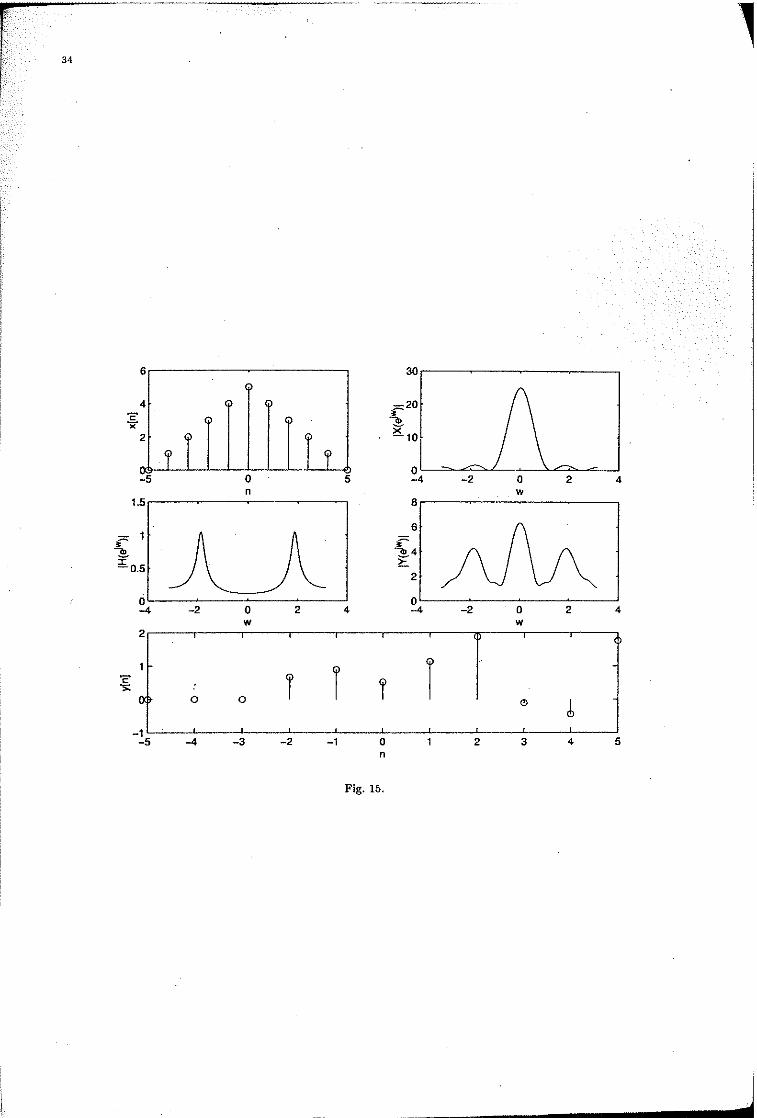
Let a filter be characterized by the difference equation
4y[n-2]+2y[n-1]+3y[n]=x[n-2], frequency response of the filter is -21..,
H(eJW) = 3+2e e'"'+4e-21w \
and ±[n] is a triangle , -5 (n (5 . We want to find the output y[n] and its frequency response,

33
Y(e1w).
The following code solves the problem and plots the graphs.
x=[O 1 2 3 4 5 4 3 2 1 OJ; 'Yodefine x[n]
n=[-5:5]; %define n's
subplot(3,2,1);
stem(n,x); %plot x[n]
xlabel(' n') ;ylabel ( 'x[ n J ');
X=fftshift(fft(x,256)); %find frequency response
w=linspace(-pi,pi,256); %take 256 points between -7r&7r
subplot(3,2,2);
plot(w,abs(X)); %plot the magnitude of the Freq. response ofx[n]
xlabel('w');ylabel('IX( e 'jw JI');
H=exp(-2*j. *w)./( 4*exp(-j. *w). '2+2*exp(-j.*w)+3);%Freq. response of the filter
subplot(3,2,3);
plot( w ,abs(H)); %::ilot the magnitude Gf the frequency response
xlabel('w');ylabel('IH( e 'jw) I');
y=filter([O 0 2],[3 2 4],x);%filter the input
subplot(3,2,4);
plot(w,abs(fftshift(fft(y,256))));% find and plot the freq. response of output
xlabel('w');ylabel('IY( e 'jw) I');
subplot(3,l,3); % we used a trick here
stem(n,y); %plot the output
xlabel('n ') ;ylabel( 'y[n] ');
--~\' ' '()' ,,
The output of the code is in Figur<i 15, x[n], IX(eiw)I, IH(&w)I, IY(eiw)/ and y[n] are plotted.
The filter is a band pass filter and~~~ngthens the signals around center frequencies, while other
frequency components are attenuated.
. I
-------~····---·--------
34
6
4 ,, ()
' ' 2 )
r r -5 0 5
n 1.5
{" 1
":!. ;;. 0.5
0 -4 -2 0 2 4
w 2 ' ' .
~ i 0• 0 0 r -1
. -5 -4 -3 -2 -1 0
n
Fig. 15.
30
·~20
g: 10
0 -4 -2
8
6
·~4 ~
2
0 -4 -2
' "
r . 2
0 w
0 w
'
3
2 4
2 4
' •D
-
.!, . 4 5


