Matching Methods for Causal Inference:A Review and a Look ForwardElizabeth A. Stuart
Abstract. When estimating causal effects using observational data, it is de-sirable to replicate a randomized experiment as closely as possible by ob-taining treated and control groups with similar covariate distributions. Thisgoal can often be achieved by choosing well-matched samples of the originaltreated and control groups, thereby reducing bias due to the covariates. Sincethe 1970s, work on matching methods has examined how to best choosetreated and control subjects for comparison. Matching methods are gainingpopularity in fields such as economics, epidemiology, medicine and politicalscience. However, until now the literature and related advice has been scat-tered across disciplines. Researchers who are interested in using matchingmethods—or developing methods related to matching—do not have a singleplace to turn to learn about past and current research. This paper providesa structure for thinking about matching methods and guidance on their use,coalescing the existing research (both old and new) and providing a summaryof where the literature on matching methods is now and where it should beheaded.
Key words and phrases: Observational study, propensity scores, subclassi-fication, weighting.
1. INTRODUCTION
One of the key benefits of randomized experimentsfor estimating causal effects is that the treated andcontrol groups are guaranteed to be only randomlydifferent from one another on all background covari-ates, both observed and unobserved. Work on matchingmethods has examined how to replicate this as muchas possible for observed covariates with observational(nonrandomized) data. Since early work in matching,which began in the 1940s, the methods have increasedin both complexity and use. However, while the fieldis expanding, there has been no single source of infor-mation for researchers interested in an overview of themethods and techniques available, nor a summary ofadvice for applied researchers interested in implement-ing these methods. In contrast, the research and re-sources have been scattered across disciplines such as
Elizabeth A. Stuart is Assistant Professor, Departments ofMental Health and Biostatistics, Johns Hopkins BloombergSchool of Public Health, Baltimore, Maryland 21205, USA(e-mail: [email protected]).
statistics (Rosenbaum, 2002; Rubin, 2006), epidemiol-ogy (Brookhart et al., 2006), sociology (Morgan andHarding, 2006), economics (Imbens, 2004) and polit-ical science (Ho et al., 2007). This paper coalescesthe diverse literature on matching methods, bringingtogether the original work on matching methods—ofwhich many current researchers are not aware—andtying together ideas across disciplines. In addition toproviding guidance on the use of matching methods,the paper provides a view of where research on match-ing methods should be headed.
We define “matching” broadly to be any method thataims to equate (or “balance”) the distribution of co-variates in the treated and control groups. This mayinvolve 1 : 1 matching, weighting or subclassification.The use of matching methods is in the broader con-text of the careful design of nonexperimental studies(Rosenbaum, 1999, 2002; Rubin, 2007). While exten-sive time and effort is put into the careful design of ran-domized experiments, relatively little effort is put intothe corresponding “design” of nonexperimental stud-ies. In fact, precisely because nonexperimental studiesdo not have the benefit of randomization, they require
even more careful design. In this spirit of design, wecan think of any study aiming to estimate the effect ofsome intervention as having two key stages: (1) design,and (2) outcome analysis. Stage (1) uses only back-ground information on the individuals in the study, de-signing the nonexperimental study as would be a ran-domized experiment, without access to the outcomevalues. Matching methods are a key tool for stage (1).Only after stage (1) is finished does stage (2) begin,comparing the outcomes of the treated and control in-dividuals. While matching is generally used to estimatecausal effects, it is also sometimes used for noncausalquestions, for example, to investigate racial disparities(Schneider, Zaslavsky and Epstein, 2004).
Alternatives to matching methods include adjustingfor background variables in a regression model, instru-mental variables, structural equation modeling or se-lection models. Matching methods have a few key ad-vantages over those other approaches. First, matchingmethods should not be seen in conflict with regressionadjustment and, in fact, the two methods are comple-mentary and best used in combination. Second, match-ing methods highlight areas of the covariate distribu-tion where there is not sufficient overlap between thetreatment and control groups, such that the resultingtreatment effect estimates would rely heavily on ex-trapolation. Selection models and regression modelshave been shown to perform poorly in situations wherethere is insufficient overlap, but their standard diag-nostics do not involve checking this overlap (Dehejiaand Wahba, 1999, 2002; Glazerman, Levy and My-ers, 2003). Matching methods in part serve to make re-searchers aware of the quality of resulting inferences.Third, matching methods have straightforward diag-nostics by which their performance can be assessed.
The paper proceeds as follows. The remainder ofSection 1 provides an introduction to matching meth-ods and the scenarios considered, including some ofthe history and theory underlying matching methods.Sections 2–5 provide details on each of the steps in-volved in implementing matching: defining a distancemeasure, doing the matching, diagnosing the matching,and then estimating the treatment effect after match-ing. The paper concludes with suggestions for futureresearch and practical guidance in Section 6.
1.1 Two Settings
Matching methods are commonly used in two typesof settings. The first is one in which the outcome valuesare not yet available and matching is used to select sub-jects for follow-up (e.g., Reinisch et al., 1995; Stuart
and Ialongo, 2009). It is particularly relevant for stud-ies with cost considerations that prohibit the collectionof outcome data for the full control group. This was thesetting for most of the original work in matching meth-ods, particularly the theoretical developments, whichcompared the benefits of selecting matched versus ran-dom samples of the control group (Althauser and Ru-bin, 1970; Rubin, 1973a, 1973b). The second setting isone in which all of the outcome data is already avail-able, and the goal of the matching is to reduce bias inthe estimation of the treatment effect.
A common feature of matching methods, which isautomatic in the first setting but not the second, isthat the outcome values are not used in the matchingprocess. Even if the outcome values are available at thetime of the matching, the outcome values should notbe used in the matching process. This precludes the se-lection of a matched sample that leads to a desired re-sult, or even the appearance of doing so (Rubin, 2007).The matching can thus be done multiple times and thematched samples with the best balance—the most sim-ilar treated and control groups—are chosen as the fi-nal matched samples; this is similar to the design ofa randomized experiment where a particular random-ization may be rejected if it yields poor covariate bal-ance (Hill, Rubin and Thomas, 1999; Greevy et al.,2004).
This paper focuses on settings with a treatment de-fined at some particular point in time, covariates mea-sured at (or relevant to) some period of time before thetreatment, and outcomes measured after the treatment.It does not consider more complex longitudinal settingswhere individuals may go in and out of the treatmentgroup, or where treatment assignment date is undefinedfor the control group. Methods such as marginal struc-tural models (Robins, Hernan and Brumback, 2000)or balanced risk set matching (Li, Propert and Rosen-baum, 2001) are useful in those settings.
1.2 Notation and Background: EstimatingCausal Effects
As first formalized in Rubin (1974), the estimationof causal effects, whether from a randomized experi-ment or a nonexperimental study, is inherently a com-parison of potential outcomes. In particular, the causaleffect for individual i is the comparison of individuali’s outcome if individual i receives the treatment (thepotential outcome under treatment), Yi(1), and individ-ual i’s outcome if individual i receives the control (thepotential outcome under control), Yi(0). For simplicity,we use the term “individual” to refer to the units that
MATCHING METHODS 3
receive the treatment of interest, but the formulationwould stay the same if the units were schools or com-munities. The “fundamental problem of causal infer-ence” (Holland, 1986) is that, for each individual, wecan observe only one of these potential outcomes, be-cause each unit (each individual at a particular point intime) will receive either treatment or control, not both.The estimation of causal effects can thus be thoughtof as a missing data problem (Rubin, 1976a), wherewe are interested in predicting the unobserved poten-tial outcomes.
For efficient causal inference and good estimation ofthe unobserved potential outcomes, we would like tocompare treated and control groups that are as similaras possible. If the groups are very different, the pre-diction of Y(1) for the control group will be made us-ing information from individuals who look very dif-ferent from themselves, and likewise for the predictionof Y(0) for the treated group. A number of authors,including Cochran and Rubin (1973), Rubin (1973a,1973b), Rubin (1979), Heckman, Ichimura and Todd(1998), Rubin and Thomas (2000) and Rubin (2001),have shown that methods such as linear regression ad-justment can actually increase bias in the estimatedtreatment effect when the true relationship betweenthe covariate and outcome is even moderately nonlin-ear, especially when there are large differences in themeans and variances of the covariates in the treated andcontrol groups.
Randomized experiments use a known randomizedassignment mechanism to ensure “balance” of thecovariates between the treated and control groups:The groups will be only randomly different fromone another on all covariates, observed and unob-served. In nonexperimental studies, we must posit anassignment mechanism, which determines which in-dividuals receive treatment and which receive con-trol. A key assumption in nonexperimental studiesis that of a strongly ignorable treatment assignment(Rosenbaum and Rubin, 1983b) which implies that(1) treatment assignment (T ) is independent of the po-tential outcomes (Y(0), Y (1)) given the covariates (X):T ⊥(Y (0), Y (1))|X, and (2) there is a positive prob-ability of receiving each treatment for all values ofX: 0 < P(T = 1|X) < 1 for all X. The first compo-nent of the definition of strong ignorability is some-times termed “ignorable,” “no hidden bias” or “uncon-founded.” Weaker versions of the ignorability assump-tion are sufficient for some quantities of interest, asdiscussed further in Imbens (2004). This assumption isoften more reasonable than it may sound at first since
matching on or controlling for the observed covariatesalso matches on or controls for the unobserved covari-ates, in so much as they are correlated with those thatare observed. Thus, the only unobserved covariates ofconcern are those unrelated to the observed covariates.Analyses can be done to assess sensitivity of the resultsto the existence of an unobserved confounder related toboth treatment assignment and the outcome (see Sec-tion 6.1.2). Heller, Rosenbaum and Small (2009) alsodiscuss how matching can make effect estimates lesssensitive to an unobserved confounder, using a conceptcalled “design sensitivity.” An additional assumption isthe Stable Unit Treatment Value Assumption (SUTVA;Rubin, 1980), which states that the outcomes of oneindividual are not affected by treatment assignment ofany other individuals. While not always plausible—for example, in school settings where treatment andcontrol children may interact, leading to “spillover”effects—the plausibility of SUTVA can often be im-proved by design, such as by reducing interactions be-tween the treated and control groups. Recent work hasalso begun thinking about how to relax this assump-tion in analyses (Hong and Raudenbush, 2006; Sobel,2006; Hudgens and Halloran, 2008).
To formalize, using notation similar to that in Rubin(1976b), we consider two populations, Pt and Pc,where the subscript t refers to a group exposed to thetreatment and c refers to a group exposed to the control.Covariate data on p pre-treatment covariates is avail-able on random samples of sizes Nt and Nc from Pt
and Pc. The means and variance covariance matrix ofthe p covariates in group i are given by μi and �i , re-spectively (i = t, c). For individual j , the p covariatesare denoted by Xj , treatment assignment by Tj (Tj = 0or 1), and the observed outcome by Yj . Without loss ofgenerality, we assume Nt < Nc.
To define the treatment effect, let E(Y (1)|X) =R1(X) and E(Y (0)|X) = R0(X). In the matching con-text effects are usually defined as the difference inpotential outcomes, τ(x) = R1(x) − R0(x), althoughother quantities, such as odds ratios, are also some-times of interest. It is often assumed that the re-sponse surfaces, R0(x) and R1(x), are parallel, so thatτ(x) = τ for all x. If the response surfaces are not par-allel (i.e., the effect varies), an average effect over somepopulation is generally estimated. Variation in effectsis particularly relevant when the estimands of interestare not difference in means, but rather odds ratios orrelative risks, for which the conditional and marginaleffects are not necessarily equal (Austin, 2007; Lunt
4 E. A. STUART
et al., 2009). The most common estimands in nonex-perimental studies are the “average effect of the treat-ment on the treated” (ATT), which is the effect forthose in the treatment group, and the “average treat-ment effect” (ATE), which is the effect on all individu-als (treatment and control). See Imbens (2004), Kurthet al. (2006) and Imai, King and Stuart (2008) for fur-ther discussion of these distinctions. The choice be-tween these estimands will likely involve both substan-tive reasons and data availability, as further discussedin Section 6.2.
1.3 History and Theoretical Development ofMatching Methods
Matching methods have been in use since the firsthalf of the 20th Century (e.g., Greenwood, 1945;Chapin, 1947), however, a theoretical basis for thesemethods was not developed until the 1970s. This de-velopment began with papers by Cochran and Rubin(1973) and Rubin (1973a, 1973b) for situations withone covariate and an implicit focus on estimating theATT. Althauser and Rubin (1970) provide an early andexcellent discussion of some practical issues associ-ated with matching: how large the control “reservoir”should be to get good matches, how to define the qual-ity of matches, how to define a “close-enough” match.Many of the issues identified in that work are topicsof continuing debate and discussion. The early papersshowed that when estimating the ATT, better matchingscenarios include situations with many more controlthan treated individuals, small initial bias between thegroups, and smaller variance in the treatment groupthan the control group.
Dealing with multiple covariates was a challenge dueto both computational and data problems. With morethan just a few covariates, it becomes very difficult tofind matches with close or exact values of all covari-ates. For example, Chapin (1947) finds that with initialpools of 671 treated and 523 controls there are only 23pairs that match exactly on six categorical covariates.An important advance was made in 1983 with the intro-duction of the propensity score, defined as the proba-bility of receiving the treatment given the observed co-variates (Rosenbaum and Rubin, 1983b). The propen-sity score facilitates the construction of matched setswith similar distributions of the covariates, without re-quiring close or exact matches on all of the individualvariables.
In a series of papers in the 1990s, Rubin and Thomas(1992a, 1992b, 1996) provided a theoretical basis formultivariate settings with affinely invariant matching
methods and ellipsoidally symmetric covariate distri-butions (such as the normal or t-distribution), againfocusing on estimating the ATT. Affinely invariantmatching methods, such as propensity score or Maha-lanobis metric matching, are those that yield the samematches following an affine (linear) transformation ofthe data. Matching in this general setting is shown to beEqual Percent Bias Reducing (EPBR; Rubin, 1976b).Rubin and Stuart (2006) later showed that the EPBRfeature also holds under much more general settings, inwhich the covariate distributions are discriminant mix-tures of ellipsoidally symmetric distributions. EPBRmethods reduce bias in all covariate directions (i.e.,makes the covariate means closer) by the same amount,ensuring that if close matches are obtained in some di-rection (such as the propensity score), then the match-ing is also reducing bias in all other directions. Thematching thus cannot be increasing bias in an outcomethat is a linear combination of the covariates. In addi-tion, matching yields the same percent bias reductionin bias for any linear function of X if and only if thematching is EPBR.
Rubin and Thomas (1992b) and Rubin and Thomas(1996) obtain analytic approximations for the reduc-tion in bias on an arbitrary linear combination of thecovariates (e.g., the outcome) that can be obtainedwhen matching on the true or estimated discriminant(or propensity score) with normally distributed covari-ates. In fact, the approximations hold remarkably welleven when the distributional assumptions are not satis-fied (Rubin and Thomas, 1996). The approximationsin Rubin and Thomas (1996) can be used to deter-mine in advance the bias reduction that will be pos-sible from matching, based on the covariate distribu-tions in the treated and control groups, the size of theinitial difference in the covariates between the groups,the original sample sizes, the number of matches de-sired and the correlation between the covariates andthe outcome. Unfortunately these approximations arerarely used in practice, despite their ability to help re-searchers quickly assess whether their data will be use-ful for estimating the causal effect of interest.
1.4 Steps in Implementing Matching Methods
Matching methods have four key steps, with thefirst three representing the “design” and the fourth the“analysis”:
1. Defining “closeness”: the distance measure used todetermine whether an individual is a good match foranother.
MATCHING METHODS 5
2. Implementing a matching method, given that mea-sure of closeness.
3. Assessing the quality of the resulting matched sam-ples, and perhaps iterating with steps 1 and 2 untilwell-matched samples result.
4. Analysis of the outcome and estimation of the treat-ment effect, given the matching done in step 3.
The next four sections go through these steps one at atime, providing an overview of approaches and adviceon the most appropriate methods.
2. DEFINING CLOSENESS
There are two main aspects to determining the mea-sure of distance (or “closeness”) to use in matching.The first involves which covariates to include, and thesecond involves combining those covariates into onedistance measure.
2.1 Variables to Include
The key concept in determining which covariates toinclude in the matching process is that of strong ignor-ability. As discussed above, matching methods, and infact most nonexperimental study methods, rely on ig-norability, which assumes that there are no unobserveddifferences between the treatment and control groups,conditional on the observed covariates. To satisfy theassumption of ignorable treatment assignment, it is im-portant to include in the matching procedure all vari-ables known to be related to both treatment assignmentand the outcome (Rubin and Thomas, 1996; Heckman,Ichimura and Todd, 1998; Glazerman, Levy and My-ers, 2003; Hill, Reiter and Zanutto, 2004). Generallypoor performance is found of methods that use a rela-tively small set of “predictors of convenience,” such asdemographics only (Shadish, Clark and Steiner, 2008).When matching using propensity scores, detailed be-low, there is little cost to including variables that areactually unassociated with treatment assignment, asthey will be of little influence in the propensity scoremodel. Including variables that are actually unassoci-ated with the outcome can yield slight increases in vari-ance. However, excluding a potentially important con-founder can be very costly in terms of increased bias.Researchers should thus be liberal in terms of includingvariables that may be associated with treatment assign-ment and/or the outcomes. Some examples of matchinghave 50 or even 100 covariates included in the proce-dure (e.g., Rubin, 2001). However, in small samplesit may not be possible to include a very large set of
variables. In that case priority should be given to vari-ables believed to be related to the outcome, as there is ahigher cost in terms of increased variance of includingvariables unrelated to the outcome but highly related totreatment assignment (Brookhart et al., 2006). Anothereffective strategy is to include a small set of covari-ates known to be related to the outcomes of interest, dothe matching, and then check the balance on all of theavailable covariates, including any additional variablesthat remain particularly unbalanced after the matching.To avoid allegations of variable selection based on esti-mated effects, it is best if the variable selection processis done without using the observed outcomes, and in-stead is based on previous research and scientific un-derstanding (Rubin, 2001).
One type of variable that should not be included inthe matching process is any variable that may havebeen affected by the treatment of interest (Rosenbaum,1984; Frangakis and Rubin, 2002; Greenland, 2003).This is especially important when the covariates, treat-ment indicator and outcomes are all collected at thesame point in time. If it is deemed to be critical tocontrol for a variable potentially affected by treat-ment assignment, it is better to exclude that variable inthe matching procedure and include it in the analysismodel for the outcome (as in Reinisch et al., 1995).1
Another challenge that potentially arises is whenvariables are fully (or nearly fully) predictive of treat-ment assignment. Excluding such a variableshould be done only with great care, with the beliefthat the problematic variable is completely unassoci-ated with the outcomes of interest and that the ignora-bility assumption will still hold. More commonly, sucha variable indicates a fundamental problem in estimat-ing the effect of interest, whereby it may not be possi-ble to separate out the effect of the treatment of interestfrom this problematic variable using the data at hand.For example, if all adolescent heavy drug users are alsoheavy drinkers, it will be impossible to separate out theeffect of heavy drug use from the effect of heavy drink-ing.
2.2 Distance Measures
The next step is to define the “distance”: a mea-sure of the similarity between two individuals. There
1The method is misstated in the footnote in Table 1 of that pa-per. In fact, the potential confounding variables were not used inthe matching procedure, but were utilized in the outcome analysis(D. B. Rubin, personal communication).
6 E. A. STUART
are four primary ways to define the distance Dij be-tween individuals i and j for matching, all of whichare affinely invariant:
1. Exact:
Dij ={ 0, if Xi = Xj ,
∞, if Xi �= Xj .
2. Mahalanobis:
Dij = (Xi − Xj)′�−1(Xi − Xj).
If interest is in the ATT, � is the variance covariancematrix of X in the full control group; if interest is inthe ATE, then � is the variance covariance matrixof X in the pooled treatment and full control groups.If X contains categorical variables, they should beconverted to a series of binary indicators, althoughthe distance works best with continuous variables.
3. Propensity score:
Dij = |ei − ej |,where ek is the propensity score for individual k,defined in detail below.
4. Linear propensity score:
Dij = | logit(ei) − logit(ej )|.Rosenbaum and Rubin (1985b), Rubin and Thomas(1996) and Rubin (2001) have found that matchingon the linear propensity score can be particularlyeffective in terms of reducing bias.
Below we use “propensity score” to refer to either thepropensity score itself or the linear version.
Although exact matching is in many ways the ideal(Imai, King and Stuart, 2008), the primary difficultywith the exact and Mahalanobis distance measures isthat neither works very well when X is high dimen-sional. Requiring exact matches often leads to many in-dividuals not being matched, which can result in largerbias than if the matches are inexact but more individ-uals remain in the analysis (Rosenbaum and Rubin,1985b). A recent advance, coarsened exact matching(CEM), can be used to do exact matching on broaderranges of the variables; for example, using incomecategories rather than a continuous measure (Iacus,King and Porro, 2009). The Mahalanobis distance canwork quite well when there are relatively few covari-ates (fewer than 8; Rubin, 1979; Zhao, 2004), but itdoes not perform as well when the covariates are notnormally distributed or there are many covariates (Guand Rosenbaum, 1993). This is likely because Maha-lanobis metric matching essentially regards all interac-tions among the elements of X as equally important;
with more covariates, Mahalanobis matching thus triesto match more and more of these multi-way interac-tions.
A major advance was made in 1983 with the intro-duction of propensity scores (Rosenbaum and Rubin,1983b). Propensity scores summarize all of the covari-ates into one scalar: the probability of being treated.The propensity score for individual i is defined as theprobability of receiving the treatment given the ob-served covariates: ei(Xi) = P(Ti = 1|Xi). There aretwo key properties of propensity scores. The first isthat propensity scores are balancing scores: At eachvalue of the propensity score, the distribution of the co-variates X defining the propensity score is the same inthe treated and control groups. Thus, grouping individ-uals with similar propensity scores replicates a mini-randomized experiment, at least with respect to the ob-served covariates. Second, if treatment assignment isignorable given the covariates, then treatment assign-ment is also ignorable given the propensity score. Thisjustifies matching based on the propensity score ratherthan on the full multivariate set of covariates. Thus,when treatment assignment is ignorable, the differencein means in the outcome between treated and controlindividuals with a particular propensity score value isan unbiased estimate of the treatment effect at thatpropensity score value. While most of the propensityscore results are in the context of finite samples andthe settings considered by Rubin and Thomas (1992a,1996), Abadie and Imbens (2009a) discuss the asymp-totic properties of propensity score matching.
The distance measures described above can also becombined, for example, doing exact matching on keycovariates such as race or gender followed by propen-sity score matching within those groups. When exactmatching on even a few variables is not possible be-cause of sample size limitations, methods that yield“fine balance” (e.g., the same proportion of AfricanAmerican males in the matched treated and controlgroups) may be a good alternative (Rosenbaum, Rossand Silber, 2007). If the key covariates of interest arecontinuous, Mahalanobis matching within propensityscore calipers (Rubin and Thomas, 2000) defines thedistance between individuals i and j as
Dij =⎧⎪⎨⎪⎩
(Zi − Zj)′�−1(Zi − Zj),
if | logit(ei) − logit(ej )| ≤ c,
∞, if | logit(ei) − logit(ej )| > c,
where c is the caliper, Z is the set of “key covari-ates,” and � is the variance covariance matrix of Z.This will yield matches that are relatively well matched
MATCHING METHODS 7
on the propensity score and particularly well matchedon Z. Z often consists of pre-treatment measures ofthe outcome, such as baseline test scores in educationalevaluations. Rosenbaum and Rubin (1985b) discuss thechoice of caliper size, generalizing results from Ta-ble 2.3.1 of Cochran and Rubin (1973). When the vari-ance of the linear propensity score in the treatmentgroup is twice as large as that in the control group,a caliper of 0.2 standard deviations removes 98% ofthe bias in a normally distributed covariate. If the vari-ance in the treatment group is much larger than thatin the control group, smaller calipers are necessary.Rosenbaum and Rubin (1985b) generally suggest acaliper of 0.25 standard deviations of the linear propen-sity score.
A more recently developed distance measure is the“prognosis score” (Hansen, 2008). Prognosis scoresare essentially the predicted outcome each individualwould have under the control condition. The benefit ofprognosis scores is that they take into account the re-lationship between the covariates and the outcome; thedrawback is that it requires a model for that relation-ship. Since it thus does not have the clear separation ofthe design and analysis stages that we advocate here,we focus instead on other approaches, but it is a poten-tially important advance in the matching literature.
2.2.1 Propensity score estimation and model spec-ification. In practice, the true propensity scores arerarely known outside of randomized experiments andthus must be estimated. Any model relating a binaryvariable to a set of predictors can be used. The mostcommon for propensity score estimation is logisticregression, although nonparametric methods such asboosted CART and generalized boosted models (gbm)often show very good performance (McCaffrey, Ridge-way and Morral, 2004; Setoguchi et al., 2008; Lee,Lessler and Stuart, 2009).
The model diagnostics when estimating propensityscores are not the standard model diagnostics for lo-gistic regression or CART. With propensity score esti-mation, concern is not with the parameter estimates ofthe model, but rather with the resulting balance of thecovariates (Augurzky and Schmidt, 2001). Because ofthis, standard concerns about collinearity do not apply.Similarly, since they do not use covariate balance as acriterion, model fit statistics identifying classificationability (such as the c-statistic) or stepwise selectionmodels are not helpful for variable selection (Rubin,2004; Brookhart et al., 2006; Setoguchi et al., 2008).One strategy that is helpful is to examine the balance
of covariates (including those not originally includedin the propensity score model), their squares and inter-actions in the matched samples. If imbalance is foundon particular variables or functions of variables, thoseterms can be included in a re-estimated propensityscore model, which should improve their balance in thesubsequent matched samples (Rosenbaum and Rubin,1984; Dehejia and Wahba, 2002).
Research indicates that misestimation of the propen-sity score (e.g., excluding a squared term that is inthe true model) is not a large problem, and that treat-ment effect estimates are more biased when the out-come model is misspecified than when the propensityscore model is misspecified (Drake, 1993; Dehejia andWahba, 1999, 2002; Zhao, 2004). This may in part bebecause the propensity score is used only as a tool toget covariate balance—the accuracy of the model isless important as long as balance is obtained. Thus, theexclusion of a squared term, for example, may haveless severe consequences for a propensity score modelthan it does for the outcome model, where interest isin interpreting a particular regression coefficient (thaton the treatment indicator). However, these evaluationsare fairly limited; for example, Drake (1993) consid-ers only two covariates. Future research should involvemore systematic evaluations of propensity score es-timation, perhaps through more sophisticated simula-tions as well as analytic work, and consideration shouldinclude how the propensity scores will be used, for ex-ample, in weighting versus subclassification.
3. MATCHING METHODS
Once a distance measure has been selected, the nextstep is to use that distance in doing the matching. Inthis section we provide an overview of the spectrumof matching methods available. The methods primar-ily vary in terms of the number of individuals that re-main after matching and in the relative weights that dif-ferent individuals receive. One way in which propen-sity scores are commonly used is as a predictor in theoutcome model, where the set of individual covari-ates is replaced by the propensity score and the out-come models run in the full treated and control groups(Weitzen et al., 2004). Unfortunately the simple use ofthis method is not an optimal use of propensity scores,as it does not take advantage of the balancing prop-erty of propensity scores: If there is imbalance on theoriginal covariates, there will also be imbalance on thepropensity score, resulting in the same degree of model
8 E. A. STUART
extrapolation as with the full set of covariates. How-ever, if the model regressing the outcome on the treat-ment indicator and the propensity score is correctlyspecified or if it includes nonlinear functions of thepropensity score (such as quantiles or splines) and theirinteraction with the treatment indicator, then this canbe an effective approach, with links to subclassifica-tion (Schafer and Kang, 2008). Since this method doesnot have the clear “design” aspect of matching, we donot discuss it further.
3.1 Nearest Neighbor Matching
One of the most common, and easiest to imple-ment and understand, methods is k : 1 nearest neighbormatching (Rubin, 1973a). This is generally the most ef-fective method for settings where the goal is to selectindividuals for follow-up. Nearest neighbor matchingnearly always estimates the ATT, as it matches controlindividuals to the treated group and discards controlswho are not selected as matches.
In its simplest form, 1 : 1 nearest neighbor match-ing selects for each treated individual i the control in-dividual with the smallest distance from individual i.A common complaint regarding 1 : 1 matching is thatit can discard a large number of observations and thuswould apparently lead to reduced power. However, thereduction in power is often minimal, for two main rea-sons. First, in a two-sample comparison of means, theprecision is largely driven by the smaller group size(Cohen, 1988). So if the treatment group stays thesame size, and only the control group decreases in size,the overall power may not actually be reduced verymuch (Ho et al., 2007). Second, the power increaseswhen the groups are more similar because of the re-duced extrapolation and higher precision that is ob-tained when comparing groups that are similar versusgroups that are quite different (Snedecor and Cochran,1980). This is also what yields the increased powerof using matched pairs in randomized experiments(Wacholder and Weinberg, 1982). Smith (1997) pro-vides an illustration where estimates from 1 : 1 match-ing have lower standard deviations than estimates froma linear regression, even though thousands of obser-vations were discarded in the matching. An additionalconcern is that, without any restrictions, k : 1 matchingcan lead to some poor matches, if, for example, thereare no control individuals with propensity scores simi-lar to a given treated individual. One strategy to avoidpoor matches is to impose a caliper and only select amatch if it is within the caliper. This can lead to dif-ficulties in interpreting effects if many treated individ-uals do not receive a match, but can help avoid poor
matches. Rosenbaum and Rubin (1985a) discuss thosetrade-offs.
3.1.1 Optimal matching. One complication of sim-ple (“greedy”) nearest neighbor matching is that theorder in which the treated subjects are matched maychange the quality of the matches. Optimal match-ing avoids this issue by taking into account the over-all set of matches when choosing individual matches,minimizing a global distance measure (Rosenbaum,2002). Generally, greedy matching performs poorlywhen there is intense competition for controls, and per-forms well when there is little competition (Gu andRosenbaum, 1993). Gu and Rosenbaum (1993) findthat optimal matching does not in general perform anybetter than greedy matching in terms of creating groupswith good balance, but does do better at reducing thedistance within pairs (page 413): “. . . optimal match-ing picks about the same controls [as greedy match-ing] but does a better job of assigning them to treatedunits.” Thus, if the goal is simply to find well-matchedgroups, greedy matching may be sufficient. However, ifthe goal is well-matched pairs, then optimal matchingmay be preferable.
3.1.2 Selecting the number of matches: Ratio match-ing. When there are large numbers of control indi-viduals, it is sometimes possible to get multiple goodmatches for each treated individual, called ratio match-ing (Smith, 1997; Rubin and Thomas, 2000). Select-ing the number of matches involves a bias :variancetrade-off. Selecting multiple controls for each treatedindividual will generally increase bias since the 2nd,3rd and 4th closest matches are, by definition, furtheraway from the treated individual than is the 1st closestmatch. On the other hand, utilizing multiple matchescan decrease variance due to the larger matched sam-ple size. Approximations in Rubin and Thomas (1996)can help determine the best ratio. In settings where theoutcome data has yet to be collected and there are costconstraints, researchers must also balance cost consid-erations. More methodological work needs to be doneto more formally quantify the trade-offs involved. Inaddition, k : 1 matching is not optimal since it doesnot account for the fact that some treated individualsmay have many close matches while others have veryfew. A more advanced form of ratio matching, variableratio matching, allows the ratio to vary, with differ-ent treated individuals receiving differing numbers ofmatches (Ming and Rosenbaum, 2001). Variable ratiomatching is related to full matching, described below.
MATCHING METHODS 9
3.1.3 With or without replacement. Another key is-sue is whether controls can be used as matches formore than one treated individual: whether the match-ing should be done “with replacement” or “without re-placement.” Matching with replacement can often de-crease bias because controls that look similar to manytreated individuals can be used multiple times. This isparticularly helpful in settings where there are few con-trol individuals comparable to the treated individuals(e.g., Dehejia and Wahba, 1999). Additionally, whenmatching with replacement, the order in which thetreated individuals are matched does not matter. How-ever, inference becomes more complex when matchingwith replacement, because the matched controls are nolonger independent—some are in the matched samplemore than once and this needs to be accounted for inthe outcome analysis, for example, by using frequencyweights. When matching with replacement, it is alsopossible that the treatment effect estimate will be basedon just a small number of controls; the number of timeseach control is matched should be monitored.
3.2 Subclassification, Full Matching and Weighting
For settings where the outcome data is already avail-able, one apparent drawback of k : 1 nearest neighbormatching is that it does not necessarily use all thedata, in that some control individuals, even some ofthose with propensity scores in the range of the treat-ment groups’ scores, are discarded and not used in theanalysis. Weighting, full matching and subclassifica-tion methods instead use all individuals. These meth-ods can be thought of as giving all individuals (ei-ther implicit or explicit) weights between 0 and 1, incontrast with nearest neighbor matching, in which in-dividuals essentially receive a weight of either 0 or1 (depending on whether or not they are selected asa match). The three methods discussed here repre-sent a continuum in terms of the number of groupingsformed, with weighting as the limit of subclassificationas the number of observations and subclasses go to in-finity (Rubin, 2001) and full matching in between.
3.2.1 Subclassification. Subclassification formsgroups of individuals who are similar, for example,as defined by quintiles of the propensity score distri-bution. It can estimate either the ATE or the ATT, asdiscussed further in Section 5. One of the first usesof subclassification was Cochran (1968), which exam-ined subclassification on a single covariate (age) in in-vestigating the link between lung cancer and smok-ing. Cochran (1968) provides analytic expressions for
the bias reduction possible using subclassification ona univariate continuous covariate; using just five sub-classes removes at least 90% of the initial bias dueto that covariate. Rosenbaum and Rubin (1985b) ex-tended that to show that creating five propensity scoresubclasses removes at least 90% of the bias in the esti-mated treatment effect due to all of the covariates thatwent into the propensity score. Based on those results,the current convention is to use 5–10 subclasses. How-ever, with larger sample sizes more subclasses (e.g.,10–20) may be feasible and appropriate (Luncefordand Davidian, 2004). More work needs to be doneto help determine the optimal number of subclasses:enough to get adequate bias reduction but not too manythat the within-subclass effect estimates become unsta-ble.
3.2.2 Full matching. A more sophisticated form ofsubclassification, full matching, selects the number ofsubclasses automatically (Rosenbaum, 1991; Hansen,2004; Stuart and Green, 2008). Full matching creates aseries of matched sets, where each matched set con-tains at least one treated individual and at least onecontrol individual (and each matched set may havemany from either group). Like subclassification, fullmatching can estimate either the ATE or the ATT. Fullmatching is optimal in terms of minimizing the aver-age of the distances between each treated individualand each control individual within each matched set.Hansen (2004) demonstrates the method in the contextof estimating the effect of SAT coaching. In that exam-ple the original treated and control groups had propen-sity score differences of 1.1 standard deviations, but thematched sets from full matching differed by only 0.01to 0.02 standard deviations. Full matching may thushave appeal for researchers who are reluctant to discardsome of the control individuals but who want to obtainoptimal balance on the propensity score. To achieve ef-ficiency gains, Hansen (2004) also introduces restrictedratios of the number of treated individuals to the num-ber of control individuals in each matched set.
3.2.3 Weighting adjustments. Propensity scores canalso be used directly as inverse weights in estimatesof the ATE, known as inverse probability of treatmentweighting (IPTW; Czajka et al., 1992; Robins, Her-nan and Brumback, 2000; Lunceford and Davidian,2004). Formally, the weight wi = Ti
ei+ 1−Ti
1−ei, where ek
is the estimated propensity score for individual k. Thisweighting serves to weight both the treated and con-trol groups up to the full sample, in the same way that
10 E. A. STUART
survey sampling weights weight a sample up to a pop-ulation (Horvitz and Thompson, 1952).
An alternative weighting technique, weighting by theodds, can be used to estimate the ATT (Hirano, Imbensand Ridder, 2003). Formally, wi = Ti + (1 − Ti)
ei
1−ei.
With this weight, treated individuals receive a weightof 1. Control individuals are weighted up to the fullsample using the 1
1−eiterm, and then weighted to the
treated group using the ei term. In this way both groupsare weighted to represent the treatment group.
A third weighting technique, used primarily in eco-nomics, is kernel weighting, which averages over mul-tiple individuals in the control group for each treatedindividual, with weights defined by their distance(Imbens, 2000). Heckman, Hidehiko and Todd (1997),Heckman et al. (1998) and Heckman, Ichimura andTodd (1998) describe a local linear matching estimatorthat requires specifying a bandwidth parameter. Gen-erally, larger bandwidths increase bias but reduce vari-ance by putting weight on individuals that are furtheraway from the treated individual of interest. A compli-cation with these methods is this need to define a band-width or smoothing parameter, which does not gener-ally have an intuitive meaning; Imbens (2004) providessome guidance on that choice.
A potential drawback of the weighting approaches isthat, as with Horvitz–Thompson estimation, the vari-ance can be very large if the weights are extreme(i.e., if the estimated propensity scores are close to 0or 1). If the model is correctly specified and thus theweights are correct, then the large variance is appro-priate. However, a worry is that some of the extremeweights may be related more to the estimation proce-dure than to the true underlying probabilities. Weighttrimming, which sets weights above some maximumto that maximum, has been proposed as one solutionto this problem (Potter, 1993; Scharfstein, Rotnitzkyand Robins, 1999). However, there is relatively lit-tle guidance regarding the trimming level. Because ofthis sensitivity to the size of the weights and potentialmodel misspecification, more attention should be paidto the accuracy of propensity score estimates whenthe propensity scores will be used for weighting vs.matching (Kang and Schafer, 2007). Another effectivestrategy is doubly-robust methods (Bang and Robins,2005), which yield accurate effect estimates if eitherthe propensity score model or the outcome model arecorrectly specified, as discussed further in Section 5.
3.3 Assessing Common Support
One issue that comes up for all matching methodsis that of “common support.” To this point, we haveassumed that there is substantial overlap of the propen-sity score distributions in the two groups, but poten-tially density differences. However, in some situationsthere may not be complete overlap in the distributions.For example, many of the control individuals may bevery different from all of the treatment group mem-bers, making them inappropriate as points of compar-ison when estimating the ATT (Austin and Mamdani,2006). Nearest neighbor matching with calipers auto-matically only uses individuals in (or close to) the areaof common support. In contrast, the subclassificationand weighting methods generally use all individuals,regardless of the overlap of the distributions. When us-ing those methods it may be beneficial to explicitly re-strict the analysis to those individuals in the region ofcommon support (as in Heckman, Hidehiko and Todd,1997; Dehejia and Wahba, 1999).
Most analyses define common support using thepropensity score, discarding individuals with propen-sity score values outside the range of the other group.A second method involves examining the “convexhull” of the covariates, identifying the multidimen-sional space that allows interpolation rather than ex-trapolation (King and Zeng, 2006). While these pro-cedures can help identify who needs to be discarded,when many subjects are discarded it can help the inter-pretation of results if it is possible to define the discardrule using one or two covariates rather than the propen-sity score itself.
It is also important to consider the implications ofcommon support for the estimand of interest. Exam-ining the common support may indicate that it is notpossible to reliably estimate the ATE. This could hap-pen, for example, if there are controls outside the rangeof the treated individuals and thus no way to esti-mate Y(1) for the controls without extensive extrapo-lation. When estimating the ATT it may be fine (and infact beneficial) to discard controls outside the range ofthe treated individuals, but discarding treated individ-uals may change the group for which the results apply(Crump et al., 2009).
4. DIAGNOSING MATCHES
Perhaps the most important step in using match-ing methods is to diagnose the quality of the resultingmatched samples. All matching should be followed byan assessment of the covariate balance in the matched
MATCHING METHODS 11
groups, where balance is defined as the similarity ofthe empirical distributions of the full set of covariatesin the matched treated and control groups. In otherwords, we would like the treatment to be unrelated tothe covariates, such that p(X|T = 1) = p(X|T = 0),where p denotes the empirical distribution. A match-ing method that results in highly imbalanced samplesshould be rejected, and alternative methods should beattempted until a well-balanced sample is attained. Insome situations the diagnostics may indicate that thetreated and control groups are too far apart to providereliable estimates without heroic modeling assump-tions (e.g., Rubin, 2001; Agodini and Dynarski, 2004).In contrast to traditional regression models, which donot examine the joint distribution of the predictors(and, in particular, of treatment assignment and the co-variates), matching methods will make it clear whenit is not possible to separate the effect of the treat-ment from other differences between the groups. Awell-specified regression model of the outcome withmany interactions would show this imbalance and maybe an effective method for estimating treatment effects(Schafer and Kang, 2008), but complex models likethat are only rarely used.
When assessing balance we would ideally comparethe multidimensional histograms of the covariates inthe matched treated and control groups. However, mul-tidimensional histograms are very coarse and/or willhave many zero cells. We thus are left examining thebalance of lower-dimensional summaries of that jointdistribution, such as the marginal distributions of eachcovariate. Since we are attempting to examine differentfeatures of the multidimensional distribution, though, itis helpful to do a number of different types of balancechecks, to obtain a more complete picture.
All balance metrics should be calculated in wayssimilar to how the outcome analyses will be run, asdiscussed further in Section 5. For example, if subclas-sification was done, the balance measures should becalculated within each subclass and then aggregated.If weights will be used in analyses (either as IPTW orbecause of variable ratio or full matching), they shouldalso be used in calculating the balance measures (Joffeet al., 2004).
4.1 Numerical Diagnostics
One of the most common numerical balance diag-nostics is the difference in means of each covariate,divided by the standard deviation in the full treated
group: Xt−Xc
σt. This measure, sometimes referred to as
the “standardized bias” or “standardized difference in
means,” is similar to an effect size and is comparedbefore and after matching (Rosenbaum and Rubin,1985b). The same standard deviation should be usedin the standardization before and after matching. Thestandardized difference of means should be computedfor each covariate, as well as two-way interactions andsquares. For binary covariates, either this same formulacan be used (treating them as if they were continuous),or a simple difference in proportions can be calculated(Austin, 2009).
Rubin (2001) presents three balance measures basedon the theory in Rubin and Thomas (1996) that providea comprehensive view of covariate balance:
1. The standardized difference of means of the propen-sity score.
2. The ratio of the variances of the propensity score inthe treated and control groups.
3. For each covariate, the ratio of the variance of theresiduals orthogonal to the propensity score in thetreated and control groups.
Rubin (2001) illustrates these diagnostics in an exam-ple with 146 covariates. For regression adjustment tobe trustworthy, the absolute standardized differencesof means should be less than 0.25 and the variance ra-tios should be between 0.5 and 2 (Rubin, 2001). Theseguidelines are based both on the assumptions underly-ing regression adjustment as well as on results in Rubin(1973b) and Cochran and Rubin (1973), which usedsimulations to estimate the bias resulting from a num-ber of treatment effect estimation procedures when thetrue relationship between the covariates and outcomeis even moderately nonlinear.
Although common, hypothesis tests and p-valuesthat incorporate information on the sample size (e.g.,t-tests) should not be used as measures of balance,for two main reasons (Austin, 2007; Imai, King andStuart, 2008). First, balance is inherently an in-sampleproperty, without reference to any broader populationor super-population. Second, hypothesis tests can bemisleading as measures of balance, because they of-ten conflate changes in balance with changes in sta-tistical power. Imai, King and Stuart (2008) show anexample where randomly discarding control individu-als seemingly leads to increased balance, simply be-cause of the reduced power. In particular, hypothesistests should not be used as part of a stopping rule to se-lect a matched sample when those samples have vary-ing sizes (or effective sample sizes). Some researchersargue that hypothesis tests are okay for testing bal-ance since the outcome analysis will also have reduced
12 E. A. STUART
power for estimating the treatment effect (Hansen,2008), but that argument requires trading off Type I andType II errors. The cost of those two types of errorsmay differ for balance checking and treatment effectestimation.
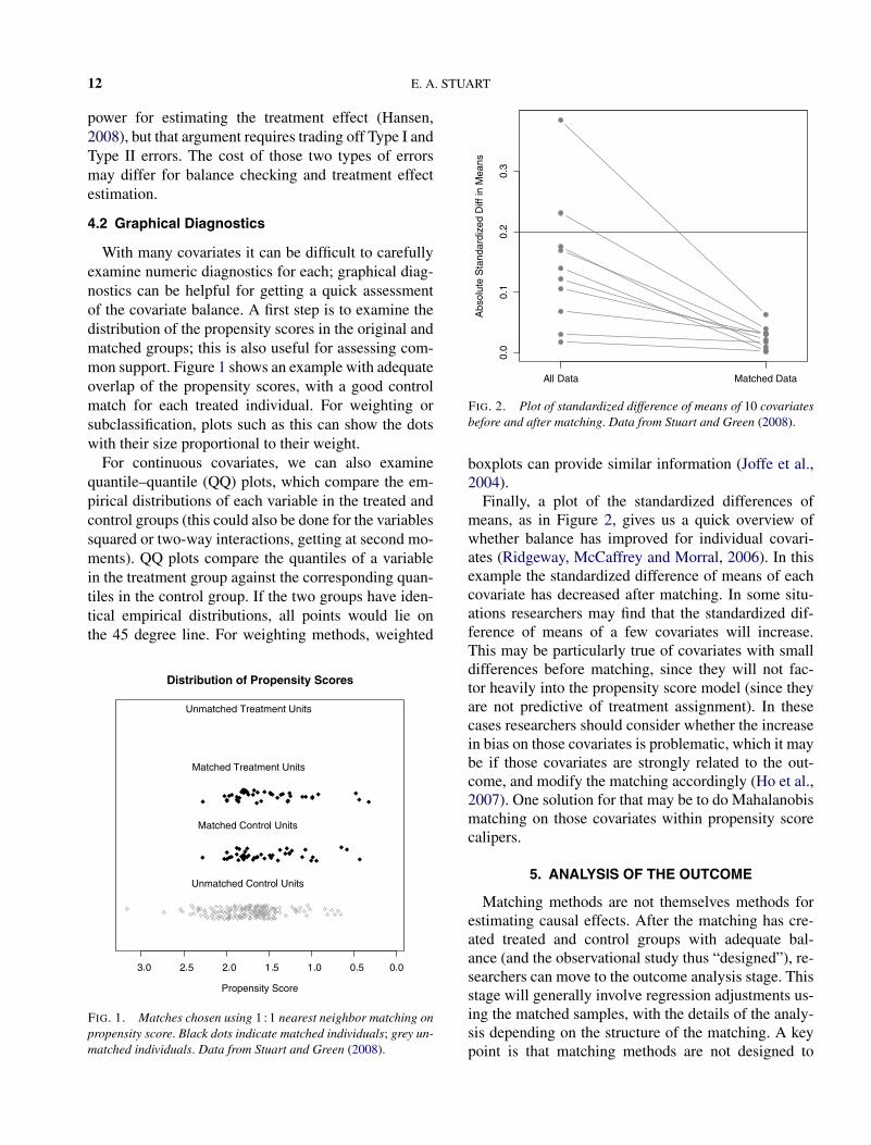
4.2 Graphical Diagnostics
With many covariates it can be difficult to carefullyexamine numeric diagnostics for each; graphical diag-nostics can be helpful for getting a quick assessmentof the covariate balance. A first step is to examine thedistribution of the propensity scores in the original andmatched groups; this is also useful for assessing com-mon support. Figure 1 shows an example with adequateoverlap of the propensity scores, with a good controlmatch for each treated individual. For weighting orsubclassification, plots such as this can show the dotswith their size proportional to their weight.
For continuous covariates, we can also examinequantile–quantile (QQ) plots, which compare the em-pirical distributions of each variable in the treated andcontrol groups (this could also be done for the variablessquared or two-way interactions, getting at second mo-ments). QQ plots compare the quantiles of a variablein the treatment group against the corresponding quan-tiles in the control group. If the two groups have iden-tical empirical distributions, all points would lie onthe 45 degree line. For weighting methods, weighted
FIG. 1. Matches chosen using 1 : 1 nearest neighbor matching onpropensity score. Black dots indicate matched individuals; grey un-matched individuals. Data from Stuart and Green (2008).
FIG. 2. Plot of standardized difference of means of 10 covariatesbefore and after matching. Data from Stuart and Green (2008).
boxplots can provide similar information (Joffe et al.,2004).
Finally, a plot of the standardized differences ofmeans, as in Figure 2, gives us a quick overview ofwhether balance has improved for individual covari-ates (Ridgeway, McCaffrey and Morral, 2006). In thisexample the standardized difference of means of eachcovariate has decreased after matching. In some situ-ations researchers may find that the standardized dif-ference of means of a few covariates will increase.This may be particularly true of covariates with smalldifferences before matching, since they will not fac-tor heavily into the propensity score model (since theyare not predictive of treatment assignment). In thesecases researchers should consider whether the increasein bias on those covariates is problematic, which it maybe if those covariates are strongly related to the out-come, and modify the matching accordingly (Ho et al.,2007). One solution for that may be to do Mahalanobismatching on those covariates within propensity scorecalipers.
5. ANALYSIS OF THE OUTCOME
Matching methods are not themselves methods forestimating causal effects. After the matching has cre-ated treated and control groups with adequate bal-ance (and the observational study thus “designed”), re-searchers can move to the outcome analysis stage. Thisstage will generally involve regression adjustments us-ing the matched samples, with the details of the analy-sis depending on the structure of the matching. A keypoint is that matching methods are not designed to
MATCHING METHODS 13
“compete” with modeling adjustments such as linearregression, and, in fact, the two methods have beenshown to work best in combination (Rubin, 1973b;Carpenter, 1977; Rubin, 1979; Robins and Rotnitzky,1995; Heckman, Hidehiko and Todd, 1997; Rubin andThomas, 2000; Glazerman, Levy and Myers, 2003;Abadie and Imbens, 2006). This is similar to the ideaof “double robustness,” and the intuition is the same asthat behind regression adjustment in randomized ex-periments, where the regression adjustment is used to“clean up” small residual covariate imbalance betweenthe groups. Matching methods should also make thetreatment effect estimates less sensitive to particularoutcome model specifications (Ho et al., 2007).
The following sections describe how outcome analy-ses should proceed after each of the major types ofmatching methods described above. When weight-ing methods are used, the weights are used directlyin regression models, for example, using weightedleast squares. We focus on parametric modeling ap-proaches since those are the most commonly used,however, nonparametric permutation-based tests, suchas Fisher’s exact test, are also appropriate, as de-tailed in Rosenbaum (2002, 2010). The best resultsare found when estimating marginal treatment effects,such as differences in means or differences in propor-tions. Greenland, Robins and Pearl (1999) and Austin(2007) discuss some of the challenges in estimatingnoncollapsible conditional treatment effects and whichmatching methods perform best for those situations.
5.1 After k : 1 Matching
When each treated individual has received k
matches, the outcome analysis proceeds using thematched samples, as if those samples had been gen-erated through randomization. There is debate aboutwhether the analysis needs to account for the matchedpair nature of the data (Austin, 2007). However, thereare at least two reasons why it is not necessary toaccount for the matched pairs (Schafer and Kang,2008; Stuart, 2008). First, conditioning on the vari-ables that were used in the matching process (suchas through a regression model) is sufficient. Second,propensity score matching, in fact, does not guaran-tee that the individual pairs will be well-matched onthe full set of covariates, only that groups of individ-uals with similar propensity scores will have similarcovariate distributions. Thus, it is more common tosimply pool all the matches into matched treated andcontrol groups and run analyses using the groups as awhole, rather than using the individual matched pairs.
In essence, researchers can do the exact same analysisthey would have done using the original data, but usingthe matched data instead (Ho et al., 2007).
Weights need to be incorporated into the analy-sis for matching with replacement or variable ratiomatching (Dehejia and Wahba, 1999; Hill, Reiter andZanutto, 2004). When matching with replacement,control group individuals receive a frequency weightthat reflects the number of times they were selectedas a match. When using variable ratio matching, con-trol group members receive a weight that is propor-tional to the number of controls matched to “their”treated individual. For example, if 1 treated individ-ual was matched to 3 controls, each of those controlsreceives a weight of 1/3. If another treated individualwas matched to just 1 control, that control receives aweight of 1.
5.2 After Subclassification or Full Matching
With standard subclassification (e.g., the formationof 5 subclasses), effects are generally estimated withineach subclass and then aggregated across subclasses(Rosenbaum and Rubin, 1984). Weighting the sub-class estimates by the number of treated individualsin each subclass estimates the ATT; weighting by theoverall number of individuals in each subclass esti-mates the ATE. There may be fairly substantial im-balance remaining in each subclass and, thus, it is im-portant to do regression adjustment within each sub-class, with the treatment indicator and covariates aspredictors (Lunceford and Davidian, 2004). When thenumber of subclasses is too large—and the numberof individuals within each subclass too small—to esti-mate separate regression models within each subclass,a joint model can be fit, with subclass and subclassby treatment indicators (fixed effects). This is espe-cially useful for full matching. This estimates a sepa-rate effect for each subclass, but assumes that the rela-tionship between the covariates X and the outcome isconstant across subclasses. Specifically, models suchas Yij = β0j + β1jTij + γXij + eij are fit, where i
indexes individuals and j indexes subclasses. In thismodel, β1j is the treatment effect for subclass j , andthese effects are aggregated across subclasses to obtainan overall treatment effect: β = Nj
N
∑Jj=1 β1j , where J
is the number of subclasses, Nj is the number of in-dividuals in subclass j , and N is the total number ofindividuals. (This formula weights subclasses by theirtotal size, and so estimates the ATE, but could be mod-ified to estimate the ATT.) This procedure is somewhatmore complicated for noncontinuous outcomes when
14 E. A. STUART
the estimand of interest, for example, an odds ratio, isnoncollapsible. In that case the outcome proportions ineach treatment group should be aggregated and thencombined.
5.3 Variance Estimation
One of the most debated topics in the literature onmatching is variance estimation. Researchers disagreeon whether uncertainty in the propensity score estima-tion or the matching procedure needs to be taken intoaccount, and, if so, how. Some researchers (e.g., Hoet al., 2007) adopt an approach similar to randomizedexperiments, where the models are run conditional onthe covariates, which are treated as fixed and exoge-nous. Uncertainty regarding the matching process isnot taken into account. Other researchers argue that un-certainty in the propensity score model needs to be ac-counted for in any analysis. However, in fact, underfairly general conditions (Rubin and Thomas, 1996;Rubin and Stuart, 2006), using estimated rather thantrue propensity scores leads to an overestimate of vari-ance, implying that not accounting for the uncertaintyin using estimated rather than true values will be con-servative in the sense of yielding confidence intervalsthat are wider than necessary. Robins, Mark and Newey(1992) also show the benefit of using estimated ratherthan true propensity scores. Analytic expressions forthe bias and variance reduction possible for these situ-ations are given in Rubin and Thomas (1992b). Specif-ically, Rubin and Thomas (1992b) states that “. . . withlarge pools of controls, matching using estimated lin-ear propensity scores results in approximately halfthe variance for the difference in the matched sam-ple means as in corresponding random samples for allcovariates uncorrelated with the population discrimi-nant.” This finding has been confirmed in simulations(Rubin and Thomas, 1996) and an empirical example(Hill, Rubin and Thomas, 1999). Thus, when it is pos-sible to obtain 100% or nearly 100% bias reduction bymatching on true or estimated propensity scores, usingthe estimated propensity scores will result in more pre-cise estimates of the average treatment effect. The in-tuition is that the estimated propensity score accountsfor chance imbalances between the groups, in additionto the systematic differences—a situation where over-fitting is good. When researchers want to account forthe uncertainty in the matching, a bootstrap procedurehas been found to outperform other methods (Lechner,2002; Hill and Reiter, 2006). There are also some em-pirical formulas for variance estimation for particularmatching scenarios (e.g., Abadie and Imbens, 2006,
2009b; Schafer and Kang, 2008), but this is an area forfuture research.
6. DISCUSSION
6.1 Additional Issues
This section raises additional issues that arise whenusing any matching method, and also provides sugges-tions for future research.
6.1.1 Missing covariate values. Most of the litera-ture on matching and propensity scores assume fullyobserved covariates, but of course most studies have atleast some missing data. One possibility is to use gen-eralized boosted models to estimate propensity scores,as they do not require fully observed covariates. An-other recommended approach is to do a simple singleimputation of the missing covariates and include miss-ing data indicators in the propensity score model. Thisessentially matches based both on the observed valuesand on the missing data patterns. Although this is gen-erally not an appropriate strategy for dealing with miss-ing data (Greenland and Finkle, 1995), it is an effec-tive approach in the propensity score context. Althoughit cannot balance the missing values themselves, thismethod will yield balance on the observed covariatesand the missing data patterns (Rosenbaum and Rubin,1984). A more flexible method is to use multiple impu-tation to impute the missing covariates, run the match-ing and effect estimation separately within each “com-plete” data set, and then use the multiple imputationcombining rules to obtain final effect estimates (Rubin,1987; Song et al., 2001). Qu and Lipkovich (2009) il-lustrate this method and show good results for an adap-tation that also includes indicators of missing data pat-terns in the propensity score model.
In addition to development and investigation ofmatching methods that account for missing data, oneparticular area needing development is balance diag-nostics for settings with missing covariate values, in-cluding dignostics that allow for nonignorable missingdata mechanisms. D’Agostino, Jr. and Rubin (2000)suggests a few simple diagnostics such as assess-ing available-case means and standard deviations ofthe continuous variables, and comparing available-case cell proportions for the categorical variables andmissing-data indicators, but diagnostics should be de-veloped that explicitly consider the interactions be-tween the missing data and treatment assignmentmechanisms.
MATCHING METHODS 15
6.1.2 Violation of ignorable treatment assignment.A critique of any nonexperimental study is that theremay be unobserved variables related to both treatmentassignment and the outcome, violating the assump-tion of ignorable treatment assignment and biasing thetreatment effect estimates. Since ignorability can neverbe directly tested, researchers have instead developedsensitivity analyses to assess its plausibility, and howviolations of ignorability may affect study conclusions.One type of plausibility test estimates an effect on avariable that is known to be unrelated to the treatment,such as a pre-treatment measure of the outcome vari-able (as in Imbens, 2004), or the difference in outcomesbetween multiple control groups (as in Rosenbaum,1987b). If the test indicates that the effect is not equalto zero, then the assumption of ignorable treatment as-signment is deemed to be less plausible.
A second approach is to perform analyses of sensi-tivity to an unobserved variable. Rosenbaum and Ru-bin (1983a) extends the ideas of Cornfield (1959),examining how strong the correlations would haveto be between a hypothetical unobserved covariateand both treatment assignment and the outcome tomake the observed treatment effect go away. Sim-ilarly, bounds can be created for the treatment ef-fect, given a range of potential correlations of theunobserved covariate with treatment assignment andthe outcome (Rosenbaum, 2002). Although sensitivityanalysis methods are becoming more and more devel-oped, they are still used relatively infrequently. Newlyavailable software (McCaffrey, Ridgeway and Morral,2004; Keele, 2009) will hopefully help facilitate theiradoption by more researchers.
6.1.3 Choosing between methods. There are a widevariety of matching methods available, and little guid-ance to help applied researchers select between them(Section 6.2 makes an attempt). The primary advice tothis point has been to select the method that yields thebest balance (e.g., Harder, Stuart and Anthony, 2010;Ho et al., 2007; Rubin, 2007). But defining the best bal-ance is complex, as it involves trading off balance onmultiple covariates. Possible ways to choose a methodinclude the following: (1) the method that yields thesmallest standardized difference of means across thelargest number of covariates, (2) the method that min-imizes the standardized difference of means of a fewparticularly prognostic covariates, and (3) the methodthat results in the fewest number of “large” standard-ized differences of means (greater than 0.25). Anotherpromising direction is work by Diamond and Sekhon
(2006), which automates the matching procedure, find-ing the best matches according to a set of balancemeasures. Further research needs to compare the per-formance of treatment effect estimates from methodsusing criteria such as those in Diamond and Sekhon(2006) and Harder, Stuart and Anthony (2010), to de-termine what the proper criteria should be and examineissues such as potential overfitting to particular mea-sures.
6.1.4 Multiple treatment doses. Throughout thisdiscussion of matching, it has been assumed that thereare just two groups: treated and control. However, inmany studies there are actually multiple levels of thetreatment (e.g., doses of a drug). Rosenbaum (2002)summarizes two methods for dealing with doses oftreatment. In the first method, the propensity scoreis still a scalar function of the covariates (e.g., Joffeand Rosenbaum, 1999; Lu et al., 2001). In the secondmethod, each of the levels of treatment has its ownpropensity score (e.g., Rosenbaum, 1987a; Imbens,2000) and each propensity score is used one at a time toestimate the distribution of responses that would havebeen observed if all individuals had received that dose.
Encompassing these two approaches, Imai and vanDyk (2004) generalizes the propensity score to arbi-trary treatment regimes (including ordinal, categori-cal and multidimensional). They provide theorems forthe properties of this generalized propensity score (thepropensity function), showing that it has propertiessimilar to that of the propensity score in that adjustingfor the low-dimensional (not always scalar, but alwayslow-dimensional) propensity function balances the co-variates. They advocate subclassification rather thanmatching, and provide two examples as well as sim-ulations showing the performance of adjustment basedon the propensity function. Diagnostics are also com-plicated in this setting, as it becomes more difficult toassess the balance of the resulting samples when thereare multiple treatment levels. Future work is needed toexamine these issues.
6.2 Guidance for Practice
So what are the take-away points and advice regard-ing when to use each of the many methods discussed?While more work is needed to definitively answer thatquestion, this section attempts to pull together the cur-rent literature to provide advice for researchers inter-ested in estimating causal effects using matching meth-ods. The lessons can be summarized as follows:
1. Think carefully about the set of covariates to in-clude in the matching procedure, and err on the side of
16 E. A. STUART
including more rather than fewer. Is the ignorability as-sumption reasonable given that set of covariates? If not,consider in advance whether there are other data setsthat may be more appropriate, or if there are sensitivityanalyses that can be done to strengthen the inferences.
2. Estimate the distance measure that will be usedin the matching. Linear propensity scores estimated us-ing logistic regression, or propensity scores estimatedusing generalized boosted models or boosted CART,are good choices. If there are a few covariates onwhich particularly close balance is desired (e.g., pre-treatment measures of the outcome), consider using theMahalanobis distance within propensity score calipers.
3. Examine the common support and implicationsfor the estimand. If the ATE is of substantive interest, isthere enough overlap of the treated and control groups’propensity scores to estimate the ATE? If not, couldthe ATT be estimated more reliably? If the ATT is ofinterest, are there controls across the full range of thetreated group, or will it be difficult to estimate the ef-fect for some treated individuals?
4. Implement a matching method.
• If estimating the ATE, good choices are generallyIPTW or full matching.
• If estimating the ATT and there are many more con-trol than treated individuals (e.g., more than 3 timesas many), k : 1 nearest neighbor matching withoutreplacement is a good choice for its simplicity andgood performance.
• If estimating the ATT and there are not (or not many)more control than treated individuals, appropriatechoices are generally subclassification, full match-ing and weighting by the odds.
5. Examine the balance on covariates resultingfrom that matching method.
• If adequate, move forward with treatment effect esti-mation, using regression adjustment on the matchedsamples.
• If imbalance on just a few covariates, consider in-corporating exact or Mahalanobis matching on thosevariables.
• If imbalance on quite a few covariates, try anothermatching method (e.g., move to k : 1 matching withreplacement) or consider changing the estimand orthe data.
Even if for some reason effect estimates will not beobtained using matching methods, it is worthwhile togo through the steps outlined here to assess the ad-equacy of the data for answering the question of in-terest. Standard regression diagnostics will not warn
researchers when there is insufficient overlap to reli-ably estimate causal effects; going through the processof estimating propensity scores and assessing balancebefore and after matching can be invaluable in termsof helping researchers move forward with causal infer-ence with confidence.
Matching methods are important tools for appliedresearchers and also have many open research ques-tions for statistical development. This paper has pro-vided an overview of the current literature on matchingmethods, guidance for practice and a road map for fu-ture research. Much research has been done in the past30 years on this topic, however, there are still a num-ber of open areas and questions to be answered. Wehope that this paper, combining results from a varietyof disciplines, will promote awareness of and interestin matching methods as an important and interestingarea for future research.
7. SOFTWARE APPENDIX
In previous years software limitations made itdifficult to implement many of the more advancedmatching methods. However, recent advances havemade these methods more and more accessible.This section lists some of the major matching pro-cedures available. A continuously updated version isalso available at http://www.biostat.jhsph.edu/~estuart/propensityscoresoftware.html.
• Matching software for R
– cem, http://gking.harvard.edu/cem/Iacus, S. M., King, G. and Porro, G. (2009). cem:Coarsened exact matching software. Can also be im-plemented through MatchIt.
– Matching, http://sekhon.berkeley.edu/matchingSekhon, J. S. (in press). Matching: Multivariate andpropensity score matching with balance optimiza-tion. Forthcoming, Journal of Statistical Software.Uses automated procedure to select matches, basedon univariate and multivariate balance diagnostics.Primarily k : 1 matching, allows matching with orwithout replacement, caliper, exact. Includes built-in effect and variance estimation procedures.
– MatchIt, http://gking.harvard.edu/matchitHo, D. E., Imai, K., King, G. and Stuart, E. A. (inpress). MatchIt: Nonparametric preprocessing forparameteric causal inference. Forthcoming, Jour-nal of Statistical Software. Two-step process: doesmatching, then user does outcome analysis. Wide ar-ray of estimation procedures and matching methods
– optmatch, http://cran.r-project.org/web/packages/optmatch/index.htmlHansen, B. B. and Fredrickson, M. (2009). opt-match: Functions for optimal matching. Variable ra-tio, optimal and full matching. Can also be imple-mented through MatchIt.
– PSAgraphics, http://cran.r-project.org/web/packages/PSAgraphics/index.htmlHelmreich, J. E. and Pruzek, R. M. (2009). PSA-graphics: Propensity score analysis graphics. Jour-nal of Statistical Software 29. Package to do graphi-cal diagnostics of propensity score methods.
– rbounds, http://cran.r-project.org/web/packages/rbounds/index.htmlKeele, L. J. (2009). rbounds: An R package for sen-sitivity analysis with matched data. Does analysis ofsensitivity to assumption of ignorable treatment as-signment.
– twang, http://cran.r-project.org/web/packages/twang/index.htmlRidgeway, G., McCaffrey, D. and Morral, A. (2006).twang: Toolkit for weighting and analysis of non-equivalent groups. Functions for propensity scoreestimating and weighting, nonresponse weighting,and diagnosis of the weights. Primarily uses gener-alized boosted regression to estimate the propensityscores.
• Matching software for Stata
– cem, http://gking.harvard.edu/cem/Iacus, S. M., King, G. and Porro, G. (2009). cem:Coarsened exact matching software.
– match, http://www.economics.harvard.edu/faculty/imbens/software_imbensAbadie, A., Drukker, D., Herr, J. L. and Imbens,G. W. (2004). Implementing matching estimators foraverage treatment effects in Stata. The Stata Journal4 290–311. Primarily k : 1 matching (with replace-ment). Allows estimation of ATT or ATE, includingrobust variance estimators.
– pscore, http://www.lrz-muenchen.de/~sobecker/pscore.htmlBecker, S. and Ichino, A. (2002). Estimation of av-erage treatment effects based on propensity scores.The Stata Journal 2 358–377. Does k : 1 nearestneighbor matching, radius (caliper) matching andsubclassification.
– psmatch2, http://econpapers.repec.org/software/bocbocode/s432001.htmLeuven, E. and Sianesi, B. (2003). psmatch2. Statamodule to perform full Mahalanobis and propen-sity score matching, common support graphing, andcovariate imbalance testing. Allows k : 1 matching,kernel weighting, Mahalanobis matching. Includesbuilt-in diagnostics and procedures for estimatingATT or ATE.
– Note: 3 procedures for analysis of sensitivity to theignorability assumption are also available: rbounds(for continuous outcomes), mhbounds (for categor-ical outcomes), and sensatt (to be used after thepscore procedures).rbounds, http://econpapers.repec.org/software/bocbocode/s438301.htm;mhbounds, http://ideas.repec.org/p/diw/diwwpp/dp659.html;sensatt, http://ideas.repec.org/c/boc/bocode/s456747.html.
• Matching software for SAS
– SAS usage note: http://support.sas.com/kb/30/971.html
– Greedy 1 : 1 matching, http://www2.sas.com/proceedings/sugi25/25/po/25p225.pdfParsons, L. S. (2005). Using SAS software to per-form a case-control match on propensity score in anobservational study. In SAS SUGI 30, Paper 225-25.
– gmatch macro, http://mayoresearch.mayo.edu/mayo/research/biostat/upload/gmatch.sasKosanke, J. and Bergstralh, E. (2004). gmatch:Match 1 or more controls to cases using theGREEDY algorithm.
– Proc assign, http://pubs.amstat.org/doi/abs/10.1198/106186001317114938Can be used to perform optimal matching.
– 1 : 1 Mahalanobis matching within propensityscore calipers, www.lexjansen.com/pharmasug/2006/publichealthresearch/pr05.pdfFeng, W. W., Jun, Y. and Xu, R. (2005). A method/macro based on propensity score and Mahalanobisdistance to reduce bias in treatment comparison inobservational study.
– vmatch macro, http://mayoresearch.mayo.edu/mayo/research/biostat/upload/vmatch.sasKosanke, J. and Bergstralh, E. (2004). Match casesto controls using variable optimal matching. Vari-able ratio matching (optimal algorithm).
Leslie, S. and Thiebaud, P. (2006). Using propensityscores to adjust for treatment selection bias.
ACKNOWLEDGMENTS
Supported in part by Award K25MH083846 fromthe National Institute of Mental Health. The contentis solely the responsibility of the author and does notnecessarily represent the official views of the NationalInstitute of Mental Health or the National Institutesof Health. The work for this paper was partially donewhile the author was a graduate student at HarvardUniversity, Department of Statistics, and a Researcherat Mathematica Policy Research. The author particu-larly thanks Jennifer Hill, Daniel Ho, Kosuke Imai,Gary King and Donald Rubin, as well as the review-ers and Editor, for helpful comments.
REFERENCES
ABADIE, A. and IMBENS, G. W. (2006). Large sample propertiesof matching estimators for average treatment effects. Economet-rica 74 235–267. MR2194325
ABADIE, A. and IMBENS, G. W. (2009a). Bias corrected matchingestimators for average treatment effects. Journal of Educationaland Behavioral Statistics. To appear. Available at http://www.hks.harvard.edu/fs/aabadie/bcm.pdf.
ABADIE, A. and IMBENS, G. W. (2009b). Matching on the esti-mated propensity score. Working Paper 15301, National Bureauof Economic Research, Cambridge, MA.
AGODINI, R. and DYNARSKI, M. (2004). Are experiments theonly option? A look at dropout prevention programs. Reviewof Economics and Statistics 86 180–194.
ALTHAUSER, R. and RUBIN, D. (1970). The computerized con-struction of a matched sample. American Journal of Sociology76 325–346.
AUGURZKY, B. and SCHMIDT, C. (2001). The propensity score:A means to an end. Discussion Paper 271, Institute for the Studyof Labor (IZA).
AUSTIN, P. C. (2007). The performance of different propensityscore methods for estimating marginal odds ratios. Stat. Med.26 3078–3094. MR2380505
AUSTIN, P. (2009). Using the standardized difference to comparethe prevalence of a binary variable between two groups in obser-vational research. Comm. Statist. Simulation Comput. 38 1228–1234.
AUSTIN, P. C. and MAMDANI, M. M. (2006). A comparisonof propensity score methods: A case-study illustrating the ef-fectiveness of post-ami statin use. Stat. Med. 25 2084–2106.MR2239634
BANG, H. and ROBINS, J. M. (2005). Doubly robust estimation inmissing data and causal inference models. Biometrics 61 962–972. MR2216189
BROOKHART, M. A., SCHNEEWEISS, S., ROTHMAN, K. J.,GLYNN, R. J., AVORN, J. and STURMER, T. (2006). Variableselection for propensity score models. American Journal of Epi-demiology 163 1149–1156.
CARPENTER, R. (1977). Matching when covariables are normallydistributed. Biometrika 64 299–307.
CHAPIN, F. (1947). Experimental Designs in Sociological Re-search. Harper, New York.
COCHRAN, W. G. (1968). The effectiveness of adjustment by sub-classification in removing bias in observational studies. Biomet-rics 24 295–313. MR0228136
COCHRAN, W. G. and RUBIN, D. B. (1973). Controlling bias inobservational studies: A review. Sankhya Ser. A 35 417–446.
COHEN, J. (1988). Statistical Power Analysis for the BehavioralSciences, 2nd ed. Earlbaum, Hillsdale, NJ.
CORNFIELD, J. (1959). Smoking and lung cancer: Recent evidenceand a discussion of some questions. Journal of the NationalCancer Institute 22 173–200.
CRUMP, R., HOTZ, V. J., IMBENS, G. W. and MITNIK, O. (2009).Dealing with limited overlap in estimation of average treatmenteffects. Biometrika 96 187–199.
CZAJKA, J. C., HIRABAYASHI, S., LITTLE, R. and RUBIN, D. B.(1992). Projecting from advance data using propensity model-ing. J. Bus. Econom. Statist. 10 117–131.
D’AGOSTINO, JR., R. B. and RUBIN, D. B. (2000). Estimatingand using propensity scores with partially missing data. J. Amer.Statist. Assoc. 95 749–759.
DEHEJIA, R. H. and WAHBA, S. (1999). Causal effects in non-experimental studies: Re-evaluating the evaluation of trainingprograms. J. Amer. Statist. Assoc. 94 1053–1062.
DEHEJIA, R. H. and WAHBA, S. (2002). Propensity score match-ing methods for non-experimental causal studies. Review ofEconomics and Statistics 84 151–161.
DIAMOND, A. and SEKHON, J. S. (2006). Genetic matchingfor estimating causal effects: A general multivariate matchingmethod for achieving balance in observational studies. Work-ing paper. Univ. California, Berkeley. Available at http://sekhon.berkeley.edu/papers/GenMatch.pdf.
DRAKE, C. (1993). Effects of misspecification of the propensityscore on estimators of treatment effects. Biometrics 49 1231–1236.
FRANGAKIS, C. E. and RUBIN, D. B. (2002). Principal stratifica-tion in causal inference. Biometrics 58 21–29. MR1891039
GLAZERMAN, S., LEVY, D. M. and MYERS, D. (2003). Nonex-perimental versus experimental estimates of earnings impacts.Annals of the American Academy of Political and Social Sci-ence 589 63–93.
GREENLAND, S. (2003). Quantifying biases in causal models:Classical confounding vs collider-stratification bias. Epidemi-ology 14 300–306.
GREENLAND, S. and FINKLE, W. D. (1995). A critical lookat methods for handling missing covariates in epidemiologicregression analyses. American Journal of Epidemiology 1421255–1264.
GREENLAND, S., ROBINS, J. M. and PEARL, J. (1999). Con-founding and collapsibility in causal inference. Statist. Sci. 1429–46.
GREENWOOD, E. (1945). Experimental Sociology: A Study inMethod. King’s Crown Press, New York.
GREEVY, R., LU, B., SILBER, J. H. and ROSENBAUM, P. (2004).Optimal multivariate matching before randomization. Biostatis-tics 5 263–275.
GU, X. and ROSENBAUM, P. R. (1993). Comparison of multivari-ate matching methods: Structures, distances, and algorithms.J. Comput. Graph. Statist. 2 405–420.
HANSEN, B. B. (2004). Full matching in an observational studyof coaching for the SAT. J. Amer. Statist. Assoc. 99 609–618.MR2086387
HANSEN, B. B. (2008). The essential role of balance testsin propensity-matched observational studies: Comments on‘A critical appraisal of propensity-score matching in the medicalliterature between 1996 and 2003’ by Peter Austin, Statistics inMedicine. Stat. Med. 27 2050–2054.
HANSEN, B. B. (2008). The prognostic analogue of the propensityscore. Biometrika 95 481–488. MR2521594
HARDER, V. S., STUART, E. A. and ANTHONY, J. (2010).Propensity score techniques and the assessment of measuredcovariate balance to test causal associations in psychological re-search. Psychological Methods. To appear.
HECKMAN, J. J., HIDEHIKO, H. and TODD, P. (1997). Matchingas an econometric evaluation estimator: Evidence from evaluat-ing a job training programme. Rev. Econom. Stud. 64 605–654.
HECKMAN, J. J., ICHIMURA, H., SMITH, J. and TODD, P. (1998).Characterizing selection bias using experimental data. Econo-metrica 66 1017–1098. MR1639419
HECKMAN, J. J., ICHIMURA, H. and TODD, P. (1998). Matchingas an econometric evaluation estimator. Rev. Econom. Stud. 65261–294. MR1623713
HELLER, R., ROSENBAUM, P. and SMALL, D. (2009). Split sam-ples and design sensitivity in observational studies. J. Amer. Sta-tist. Assoc. 104 1090–1101.
HILL, J. L. and REITER, J. P. (2006). Interval estimation for treat-ment effects using propensity score matching. Stat. Med. 252230–2256. MR2240098
HILL, J., REITER, J. and ZANUTTO, E. (2004). A comparisonof experimental and observational data analyses. In AppliedBayesian Modeling and Causal Inference From an Incomplete-Data Perspective (A. Gelman and X.-L. Meng, eds.). Wiley,Hoboken, NJ. MR2134801
HILL, J., RUBIN, D. B. and THOMAS, N. (1999). The design ofthe New York School Choice Scholarship Program evaluation.In Research Designs: Inspired by the Work of Donald Campbell,(L. Bickman, ed.) 155–180. Sage, Thousand Oaks, CA.
HIRANO, K., IMBENS, G. W. and RIDDER, G. (2003). Effi-cient estimation of average treatment effects using the estimatedpropensity score. Econometrica 71 1161–1189. MR1995826
HO, D. E., IMAI, K., KING, G. and STUART, E. A. (2007).Matching as nonparametric preprocessing for reducing modeldependence in parametric causal inference. Political Analysis15 199–236.
HOLLAND, P. W. (1986). Statistics and causal inference. J. Amer.Statist. Assoc. 81 945–960. MR0867618
HONG, G. and RAUDENBUSH, S. W. (2006). Evaluating kinder-garten retention policy: A case study of causal inference formultilevel observational data. J. Amer. Statist. Assoc. 101 901–910. MR2324091
HORVITZ, D. and THOMPSON, D. (1952). A generalization ofsampling without replacement from a finite universe. J. Amer.Statist. Assoc. 47 663–685. MR0053460
HUDGENS, M. G. and HALLORAN, M. E. (2008). Toward causalinference with interference. J. Amer. Statist. Assoc. 103 832–842. MR2435472
IACUS, S. M., KING, G. and PORRO, G. (2009). CEM: Softwarefor coarsened exact matching. J. Statist. Software 30 9. Avail-able at http://gking.harvard.edu/files/abs/cemR-abs.shtml.
IMAI, K. and VAN DYK, D. A. (2004). Causal inference withgeneral treatment regimes: Generalizing the propensity score.J. Amer. Statist. Assoc. 99 854–866. MR2090918
IMAI, K., KING, G. and STUART, E. A. (2008). Misunderstand-ings among experimentalists and observationalists in causal in-ference. J. Roy. Statist. Soc. Ser. A 171 481–502. MR2427345
IMBENS, G. W. (2000). The role of the propensity score inestimating dose–response functions. Biometrika 87 706–710.MR1789821
IMBENS, G. W. (2004). Nonparametric estimation of average treat-ment effects under exogeneity: A review. Review of Economicsand Statistics 86 4–29.
JOFFE, M. M. and ROSENBAUM, P. R. (1999). Propensity scores.American Journal of Epidemiology 150 327–333.
JOFFE, M. M., TEN HAVE, T. R., FELDMAN, H. I. and KIMMEL,S. E. (2004). Model selection, confounder control, and mar-ginal structural models. Amer. Statist. 58 272–279. MR2109415
KANG, J. D. and SCHAFER, J. L. (2007). Demystifying doublerobustness: A comparison of alternative strategies for estimatinga population mean from incomplete data. Statist. Sci. 22 523–539. MR2420458
KEELE, L. (2009). rbounds: An R package for sensitivity analysiswith matched data. R package. Available at http://www.polisci.ohio-state.edu/faculty/lkeele/rbounds.html.
KING, G. and ZENG, L. (2006). The dangers of extreme counter-factuals. Political Analysis 14 131–159.
KURTH, T., WALKER, A. M., GLYNN, R. J., CHAN, K. A.,GAZIANO, J. M., BERGER, K. and ROBINS, J. M. (2006). Re-sults of multivariable logistic regresion, propensity matching,propensity adjustment, and propensity-based weighting underconditions of nonuniform effect. American Journal of Epidemi-ology 163 262–270.
LECHNER, M. (2002). Some practical issues in the evaluation ofheterogeneous labour market programmes by matching meth-ods. J. Roy. Statist. Soc. Ser. A 165 59–82. MR1888488
LEE, B., LESSLER, J. and STUART, E. A. (2009). Improvingpropensity score weighting using machine learning. Stat. Med.29 337–346.
LI, Y. P., PROPERT, K. J. and ROSENBAUM, P. R. (2001). Bal-anced risk set matching. J. Amer. Statist. Assoc. 96 455, 870–882. MR1946360
LU, B., ZANUTTO, E., HORNIK, R. and ROSENBAUM, P. R.(2001). Matching with doses in an observational study of a me-dia campaign against drug abuse. J. Amer. Statist. Assoc. 961245–1253. MR1973668
LUNCEFORD, J. K. and DAVIDIAN, M. (2004). Stratification andweighting via the propensity score in estimation of causal treat-ment effects: A comparative study. Stat. Med. 23 2937–2960.
LUNT, M., SOLOMON, D., ROTHMAN, K., GLYNN, R., HYRICH,K., SYMMONS, D. P., STURMER, T., THE BRITISH SO-CIETY FOR RHEUMATOLOGY BIOLOGICS REGISTER andTHE BRITISH SOCIETY FOR RHEUMATOLOGY BIOLOGICS
REGISTER CONTRL CENTRE CONSORTIUM (2009). Differentmethods of balancing covariates leading to different effect esti-mates in the presence of effect modification. American Journalof Epidemiology 169 909–917.
MCCAFFREY, D. F., RIDGEWAY, G. and MORRAL, A. R. (2004).Propensity score estimation with boosted regression for evaluat-ing causal effects in observational studies. Psychological Meth-ods 9 403–425.
MING, K. and ROSENBAUM, P. R. (2001). A note on optimalmatching with variable controls using the assignment algorithm.J. Comput. Graph. Statist. 10 455–463. MR1939035
MORGAN, S. L. and HARDING, D. J. (2006). Matching estimatorsof causal effects: Prospects and pitfalls in theory and practice.Sociological Methods & Research 35 3–60. MR2247150
POTTER, F. J. (1993). The effect of weight trimming on nonlin-ear survey estimates. In Proceedings of the Section on SurveyResearch Methods of American Statistical Association. Amer.Statist. Assoc., San Francisco, CA.
QU, Y. and LIPKOVICH, I. (2009). Propensity score estimationwith missing values using a multiple imputation missingnesspattern (MIMP) approach. Stat. Med. 28 1402–1414.
REINISCH, J., SANDERS, S., MORTENSEN, E. and RUBIN, D. B.(1995). In utero exposure to phenobarbital and intelligencedeficits in adult men. Journal of the American Medical Asso-ciation 274 1518–1525.
RIDGEWAY, G., MCCAFFREY, D. and MORRAL, A. (2006).twang: Toolkit for weighting and analysis of nonequivalentgroups. Software for using matching methods in R. Availableat http://cran.r-project.org/web/packages/twang/index.html.
ROBINS, J. and ROTNITZKY, A. (1995). Semiparametric efficiencyin multivariate regression models with missing data. J. Amer.Statist. Assoc. 90 122–129. MR1325119
ROBINS, J. M., HERNAN, M. A. and BRUMBACK, B. (2000).Marginal structural models and causal inference in epidemiol-ogy. Epidemiology 11 550–560.
ROBINS, J. M., MARK, S. and NEWEY, W. (1992). Estimatingexposure effects by modelling the expectation of exposure con-ditional on confounders. Biometrics 48 479–495. MR1173493
ROSENBAUM, P. R. (1984). The consequences of adjustment fora concomitant variable that has been affected by the treatment.J. Roy. Statist. Soc. Ser. A 147 656–666.
ROSENBAUM, P. R. (1987a). Model-based direct adjustment.J. Amer. Statist. Assoc. 82 387–394.
ROSENBAUM, P. R. (1987b). The role of a second control groupin an observational study (with discussion). Statist. Sci. 2 292–316.
ROSENBAUM, P. R. (1991). A characterization of optimal designsfor observational studies. J. Roy. Statist. Soc. Ser. B 53 597–610.MR1125717
ROSENBAUM, P. R. (1999). Choice as an alternative to control inobservational studies (with discussion). Statist. Sci. 14 259–304.
ROSENBAUM, P. R. (2002). Observational Studies, 2nd ed.Springer, New York. MR1899138
ROSENBAUM, P. R. (2010). Design of Observational Studies.Springer, New York.
ROSENBAUM, P. R. and RUBIN, D. B. (1983a). Assessing sen-sitivity to an unobserved binary covariate in an observationalstudy with binary outcome. J. Roy. Statist. Soc. Ser. B 45 212–218.
ROSENBAUM, P. R. and RUBIN, D. B. (1983b). The central role ofthe propensity score in observational studies for causal effects.Biometrika 70 41–55. MR0742974
ROSENBAUM, P. R. and RUBIN, D. B. (1984). Reducing bias inobservational studies using subclassification on the propensityscore. J. Amer. Statist. Assoc. 79 516–524.
ROSENBAUM, P. R. and RUBIN, D. B. (1985a). The bias due toincomplete matching. Biometrics 41 103–116. MR0793436
ROSENBAUM, P. R. and RUBIN, D. B. (1985b). Constructing acontrol group using multivariate matched sampling methodsthat incorporate the propensity score. Amer. Statist. 39 33–38.
ROSENBAUM, P. R., ROSS, R. N. and SILBER, J. H. (2007). Min-imum distance matched sampling with fine balance in an obser-vational study of treatment for ovarian cancer. J. Amer. Statist.Assoc. 102 75–83. MR2345534
RUBIN, D. B. (1973a). Matching to remove bias in observationalstudies. Biometrics 29 159–184.
RUBIN, D. B. (1973b). The use of matched sampling and regres-sion adjustment to remove bias in observational studies. Bio-metrics 29 185–203.
RUBIN, D. B. (1974). Estimating causal effects of treatments inrandomized and nonrandomized studies. Journal of EducationalPsychology 66 688–701.
RUBIN, D. B. (1976a). Inference and missing data (with discus-sion). Biometrika 63 581–592. MR0455196
RUBIN, D. B. (1976b). Multivariate matching methods that areequal percent bias reducing, I: Some examples. Biometrics 32109–120. MR0400555
RUBIN, D. B. (1979). Using multivariate matched sampling andregression adjustment to control bias in observational studies.J. Amer. Statist. Assoc. 74 318–328.
RUBIN, D. B. (1980). Bias reduction using Mahalanobis metricmatching. Biometrics 36 293–298.
RUBIN, D. B. (1987). Multiple Imputation for Nonresponse in Sur-veys. Wiley, New York. MR0899519
RUBIN, D. B. (2001). Using propensity scores to help design ob-servational studies: Application to the tobacco litigation. HealthServices & Outcomes Research Methodology 2 169–188.
RUBIN, D. B. (2004). On principles for modeling propensityscores in medical research. Pharmacoepidemiology and DrugSafety 13 855–857.
RUBIN, D. B. (2006). Matched Sampling for Causal Inference.Cambridge Univ. Press, Cambridge. MR2307965
RUBIN, D. B. (2007). The design versus the analysis of observa-tional studies for causal effects: Parallels with the design of ran-domized trials. Stat. Med. 26 20–36. MR2312697
RUBIN, D. B. and STUART, E. A. (2006). Affinely invariantmatching methods with discriminant mixtures of proportionalellipsoidally symmetric distributions. Ann. Statist. 34 1814–1826. MR2283718
RUBIN, D. B. and THOMAS, N. (1992a). Affinely invariant match-ing methods with ellipsoidal distributions. Ann. Statist. 201079–1093. MR1165607
RUBIN, D. B. and THOMAS, N. (1992b). Characterizing the effectof matching using linear propensity score methods with normaldistributions. Biometrika 79 797–809. MR1209479
RUBIN, D. B. and THOMAS, N. (1996). Matching using estimatedpropensity scores, relating theory to practice. Biometrics 52249–264.
RUBIN, D. B. and THOMAS, N. (2000). Combining propensityscore matching with additional adjustments for prognostic co-variates. J. Amer. Statist. Assoc. 95 573–585.
SCHAFER, J. L. and KANG, J. D. (2008). Average causal effectsfrom nonrandomized studies: A practical guide and simulatedcase study. Psychological Methods 13 279–313.
SCHARFSTEIN, D. O., ROTNITZKY, A. and ROBINS, J. M.(1999). Adjusting for non-ignorable drop-out using semipara-metric non-response models. J. Amer. Statist. Assoc. 94 1096–1120. MR1731478
SCHNEIDER, E. C., ZASLAVSKY, A. M. and EPSTEIN, A. M.(2004). Use of high-cost operative procedures by Medicare ben-eficiaries enrolled in for-profit and not-for-profit health plans.The New England Journal of Medicine 350 143–150.
SETOGUCHI, S., SCHNEEWEISS, S., BROOKHART, M. A.,GLYNN, R. J. and COOK, E. F. (2008). Evaluating uses of datamining techniques in propensity score estimation: A simulationstudy. Pharmacoepidemiology and Drug Safety 17 546–555.
SHADISH, W. R., CLARK, M. and STEINER, P. M. (2008). Cannonrandomized experiments yield accurate answers? A ran-domized experiment comparing random and nonrandom assign-ments. J. Amer. Statist. Assoc. 103 1334–1344.
SMITH, H. (1997). Matching with multiple controls to estimatetreatment effects in observational studies. Sociological Method-ology 27 325–353.
SNEDECOR, G. W. and COCHRAN, W. G. (1980). StatisticalMethods, 7th ed. Iowa State Univ. Press, Ames, IA. MR0614143
SOBEL, M. E. (2006). What do randomized studies of housing mo-bility demonstrate?: Causal inference in the face of interference.J. Amer. Statist. Assoc. 101 1398–1407. MR2307573
SONG, J., BELIN, T. R., LEE, M. B., GAO, X. and ROTHERAM-BORUS, M. J. (2001). Handling baseline differences and miss-
ing items in a longitudinal study of HIV risk among runawayyouths. Health Services & Outcomes Research Methodology 2317–329.
STUART, E. A. (2008). Developing practical recommendationsfor the use of propensity scores: Discussion of “A critical ap-praisal of propensity score matching in the medical literaturebetween 1996 and 2003” by P. Austin. Stat. Med. 27 2062–2065.MR2439885
STUART, E. A. and GREEN, K. M. (2008). Using full matchingto estimate causal effects in non-experimental studies: Examin-ing the relationship between adolescent marijuana use and adultoutcomes. Developmental Psychology 44 395–406.
STUART, E. A. and IALONGO, N. S. (2009). Matching methodsfor selection of subjects for follow-up. Multivariate BehavioralResearch. To appear.
WACHOLDER, S. and WEINBERG, C. R. (1982). Paired versustwo-sample design for a clinical trial of treatments with dichoto-mous outcome: Power considerations. Biometrics 38 801–812.
WEITZEN, S., LAPANE, K. L., TOLEDANO, A. Y., HUME, A. L.and MOR, V. (2004). Principles for modeling propensity scoresin medical research: A systematic literature review. Pharma-coepidemiology and Drug Safety 13 841–853.
ZHAO, Z. (2004). Using matching to estimate treatment effects:Data requirements, matching metrics, and Monte Carlo evi-dence. Review of Economics and Statistics 86 91–107.