Math 143: Introduction to Biostatisticsrpruim/courses/m143/S11/fromClass/Math143S...X-squared =...

Math 143: Introduction to Biostatistics

R Pruim

Spring 2011

0.2

Last Modified: April 4, 2011 Math 143 : Spring 2011 : Pruim

Contents

8 Goodness of Fit Testing 18.1 Testing Simple Hypotheses . . . . . . . . . . . . . . . . . . . . . . . . . . . . . . . . . . . . . . . 18.2 Testing Complex Hypotheses . . . . . . . . . . . . . . . . . . . . . . . . . . . . . . . . . . . . . . 58.3 Reporting Results of Hypothesis Tests . . . . . . . . . . . . . . . . . . . . . . . . . . . . . . . . . 6

9 Chi-squared for Contingency Tables 1

10 Normal Distributions 110.1 The Family of Normal Distributions . . . . . . . . . . . . . . . . . . . . . . . . . . . . . . . . . . 110.2 The Central Limit Theorem . . . . . . . . . . . . . . . . . . . . . . . . . . . . . . . . . . . . . . . 310.3 Confidence Intervals . . . . . . . . . . . . . . . . . . . . . . . . . . . . . . . . . . . . . . . . . . . 6

11 Inference for the Mean of a Population 111.1 Hypothesis Tests . . . . . . . . . . . . . . . . . . . . . . . . . . . . . . . . . . . . . . . . . . . . . 111.2 Confidence Intervals . . . . . . . . . . . . . . . . . . . . . . . . . . . . . . . . . . . . . . . . . . . 311.3 Overview of One-Sample Methods . . . . . . . . . . . . . . . . . . . . . . . . . . . . . . . . . . . 3

12 Comparing Two Means 112.1 The Distinction Between Paired T and 2-sample T . . . . . . . . . . . . . . . . . . . . . . . . . . 112.2 Comparing Two Means in R . . . . . . . . . . . . . . . . . . . . . . . . . . . . . . . . . . . . . . . 212.3 Formulas for 2-Sample T . . . . . . . . . . . . . . . . . . . . . . . . . . . . . . . . . . . . . . . . . 3

3

7.4


Goodness of Fit Testing 8.1

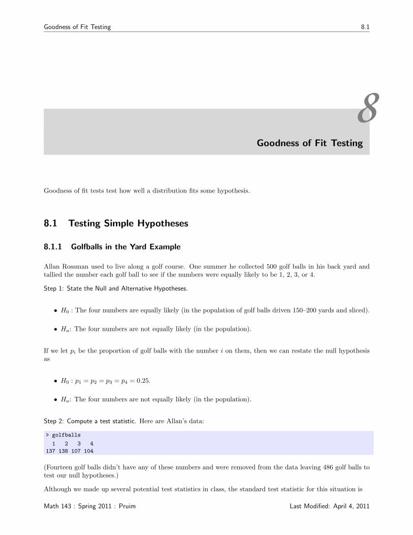
8Goodness of Fit Testing

Goodness of fit tests test how well a distribution fits some hypothesis.

8.1 Testing Simple Hypotheses

8.1.1 Golfballs in the Yard Example

Allan Rossman used to live along a golf course. One summer he collected 500 golf balls in his back yard andtallied the number each golf ball to see if the numbers were equally likely to be 1, 2, 3, or 4.

Step 1: State the Null and Alternative Hypotheses.

• H0 : The four numbers are equally likely (in the population of golf balls driven 150–200 yards and sliced).

• Ha: The four numbers are not equally likely (in the population).

If we let pi be the proportion of golf balls with the number i on them, then we can restate the null hypothesisas

• H0 : p1 = p2 = p3 = p4 = 0.25.

• Ha: The four numbers are not equally likely (in the population).

Step 2: Compute a test statistic. Here are Allan’s data:

> golfballs

1 2 3 4

137 138 107 104

(Fourteen golf balls didn’t have any of these numbers and were removed from the data leaving 486 golf balls totest our null hypotheses.)

Although we made up several potential test statistics in class, the standard test statistic for this situation is

Math 143 : Spring 2011 : Pruim Last Modified: April 4, 2011

8.2 Goodness of Fit Testing

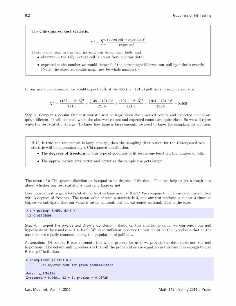
The Chi-squared test statistic:

X2 =∑ (observed− expected)2

expected

There is one term in this sum for each cell in our data table, and• observed = the tally in that cell (a count from our raw data)

• expected = the number we would “expect” if the percentages followed our null hypothesis exactly.(Note: the expected counts might not be whole numbers.)

In our particular example, we would expect 25% of the 486 (i.e., 121.5) golf balls in each category, so

X2 =(137− 121.5)2

121.5+

(138− 121.5)2

121.5+

(107− 121.5)2

121.5+

(104− 121.5)2

121.5= 8.469

Step 3: Compute a p-value Our test statistic will be large when the observed counts and expected counts arequite different. It will be small when the observed counts and expected counts are quite close. So we will rejectwhen the test statistic is large. To know how large is large enough, we need to know the sampling distribution.

If H0 is true and the sample is large enough, then the sampling distribution for the Chi-squared teststatistic will be approximately a Chi-squared distribution.

• The degrees of freedom for this type of goodness of fit test is one less than the number of cells.

• The approximation gets better and better as the sample size gets larger.

The mean of a Chi-squared distribution is equal to its degrees of freedom. This can help us get a rough ideaabout whether our test statistic is unusually large or not.

How unusual is it to get a test statistic at least as large as ours (8.47)? We compare to a Chi-squared distributionwith 3 degrees of freedom. The mean value of such a statistic is 3, and our test statistic is almost 3 times asbig, so we anticipate that our value is rather unusual, but not extremely unusual. This is the case:

> 1 - pchisq( 8.469, df=3 )

[1] 0.03725096

Step 4: Interpret the p-value and Draw a Conclusion. Based on this smallish p-value, we can reject our nullhypothesis at the usual α = 0.05 level. We have sufficient evidence to cast doubt on the hypothesis that all thenumbers are equally common among the population of golfballs.

Automation. Of course, R can automate this whole process for us if we provide the data table and the nullhypothesis. The default null hypothesis is that all the probabilities are equal, so in this case it is enough to giveR the golf balls data.

> chisq.test( golfballs )

Chi-squared test for given probabilities

data: golfballs

X-squared = 8.4691, df = 3, p-value = 0.03725



8.1.2 Plant Genetics Example

A biologist is conducting a plant breeding experiment in which plants can have one of four phenotypes. If thesephenotypes are caused by a simple Mendelian model, the phenotypes should occur in a 9:3:3:1 ratio. She raises41 plants with the following phenotypes.

phenotype 1 2 3 4

count 20 10 7 4

Should she worry that the simple genetic model doesn’t work for her phenotypes?

> plants <- c( 20, 10, 7, 4 )

> chisq.test( plants, p=c(9/16, 3/16, 3/16, 1/16) )


data: plants


Things to notice:

• plants <- c( 20, 10, 7, 4 ) is the way to enter this kind of data by hand.

• This time we need to tell R what the null hypothesis is. That’s what p=c(9/16, 3/16, 3/16, 1/16) isfor.

• The Chi-squared distribution is only an approximation to the sampling distribution of our test statistic,and the approximation is not very good when the expected cell counts are too small.

Our rule of thumb will be this:

To use the chi-squared approximation

• All the expected counts should be at least 1.

• Most (at least 80%) of the expected counts should be at least 5.

Notice that this depends on expected counts, not observed counts.

Our expected count for phenotype 4 is only 116 · 41 = 2.562, which means that 75% of our expected counts are

between 1 and 5, so our approximation will be a little crude. (The other expected counts are well in the saferange.)

When this happens, we can ask R to use the empirical method (just like we did with statTally) instead.

> chisq.test( plants, p= c(9/16, 3/16, 3/16, 1/16), simulate = T )

Chi-squared test for given probabilities with simulated p-value (based on 2000

replicates)

data: plants

X-squared = 1.9702, df = NA, p-value = 0.5932

This doesn’t change our overall conclusion in this case. These data are not inconsistent with the simple geneticmodel. (The simulated p-value is not terribly accurate either if we use only 2000 replicates. We could increasethat for more accuracy. If you repeat the code above several times, you will see how the empirical p-value variesfrom one computation to the next.)



If we had more data . . .

Interestingly, if we had 10 times as much data in the same proportions, the conclusion would be very different.

> plants <- c( 200, 100, 70, 40 )

> chisq.test( plants, p=c(9/16, 3/16, 3/16, 1/16) )


data: plants


8.1.3 When there are only two categories

We can redo our toads example using a goodness of fit test instead of the binomial test.

> binom.test(14,18)

Exact binomial test

data: 14 and 18

number of successes = 14, number of trials = 18, p-value = 0.03088

alternative hypothesis: true probability of success is not equal to 0.5

95 percent confidence interval:

0.5236272 0.9359080

sample estimates:

probability of success

0.7777778

> chisq.test(c(14,4))


data: c(14, 4)


Both of these test the same hypotheses:

• H0 : pL = pR = 0.5

• Ha : pL 6= pR

where pL and pR are proportions of right and left-handed toads in the population).

Although both tests test the same hypotheses and give similar p-values (in this example), the binomial test isgenerally used because

• The binomial test is exact for all sample sizes while the Chi-squared test is only approximate, and theapproximation is poor when sample sizes are small.

• Later we will learn about the confidence interval associated with the binomial test. This will be anotheradvantages of the binomial test over the Chi-squared test.



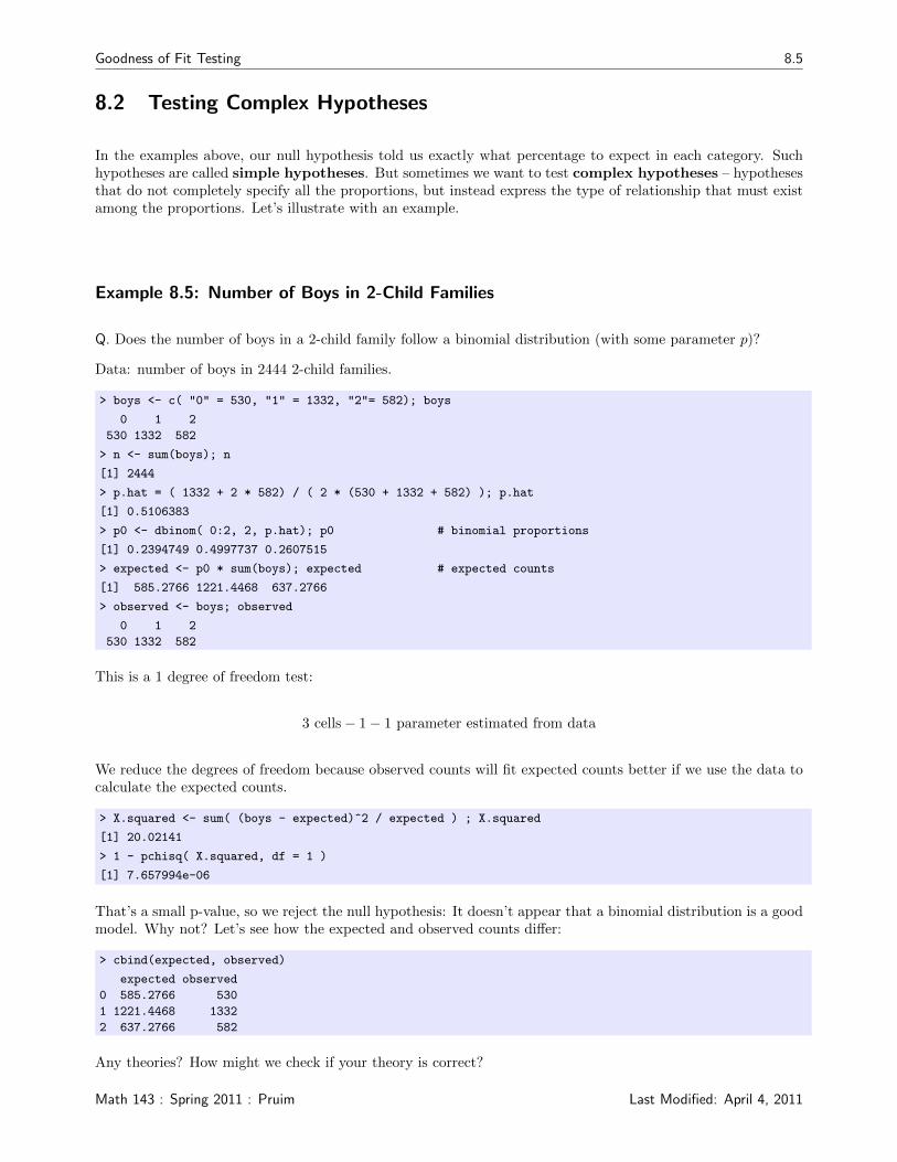
8.2 Testing Complex Hypotheses

In the examples above, our null hypothesis told us exactly what percentage to expect in each category. Suchhypotheses are called simple hypotheses. But sometimes we want to test complex hypotheses – hypothesesthat do not completely specify all the proportions, but instead express the type of relationship that must existamong the proportions. Let’s illustrate with an example.

Example 8.5: Number of Boys in 2-Child Families

Q. Does the number of boys in a 2-child family follow a binomial distribution (with some parameter p)?

Data: number of boys in 2444 2-child families.

> boys <- c( "0" = 530, "1" = 1332, "2"= 582); boys

0 1 2

530 1332 582

> n <- sum(boys); n

[1] 2444

> p.hat = ( 1332 + 2 * 582) / ( 2 * (530 + 1332 + 582) ); p.hat

[1] 0.5106383

> p0 <- dbinom( 0:2, 2, p.hat); p0 # binomial proportions

[1] 0.2394749 0.4997737 0.2607515

> expected <- p0 * sum(boys); expected # expected counts

[1] 585.2766 1221.4468 637.2766

> observed <- boys; observed

0 1 2

530 1332 582

This is a 1 degree of freedom test:

3 cells− 1− 1 parameter estimated from data

We reduce the degrees of freedom because observed counts will fit expected counts better if we use the data tocalculate the expected counts.

> X.squared <- sum( (boys - expected)^2 / expected ) ; X.squared

[1] 20.02141

> 1 - pchisq( X.squared, df = 1 )

[1] 7.657994e-06

That’s a small p-value, so we reject the null hypothesis: It doesn’t appear that a binomial distribution is a goodmodel. Why not? Let’s see how the expected and observed counts differ:

> cbind(expected, observed)

expected observed

0 585.2766 530

1 1221.4468 1332

2 637.2766 582

Any theories? How might we check if your theory is correct?



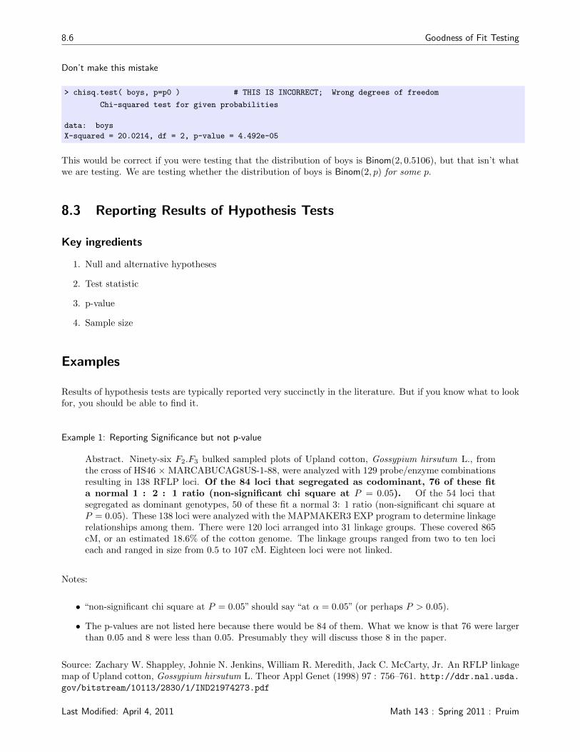
Don’t make this mistake

> chisq.test( boys, p=p0 ) # THIS IS INCORRECT; Wrong degrees of freedom


data: boys

X-squared = 20.0214, df = 2, p-value = 4.492e-05

This would be correct if you were testing that the distribution of boys is Binom(2, 0.5106), but that isn’t whatwe are testing. We are testing whether the distribution of boys is Binom(2, p) for some p.

8.3 Reporting Results of Hypothesis Tests

Key ingredients

1. Null and alternative hypotheses

2. Test statistic

3. p-value

4. Sample size

Examples

Results of hypothesis tests are typically reported very succinctly in the literature. But if you know what to lookfor, you should be able to find it.

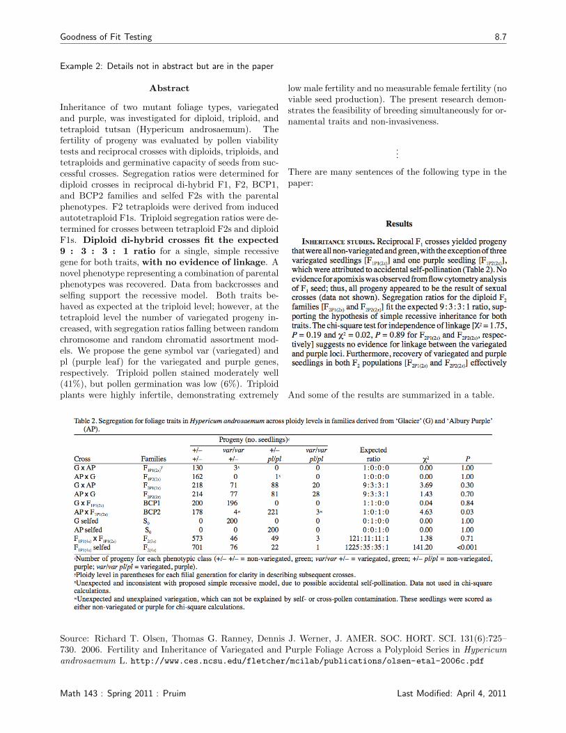
Example 1: Reporting Significance but not p-value

Abstract. Ninety-six F2.F3 bulked sampled plots of Upland cotton, Gossypium hirsutum L., fromthe cross of HS46 × MARCABUCAG8US-1-88, were analyzed with 129 probe/enzyme combinationsresulting in 138 RFLP loci. Of the 84 loci that segregated as codominant, 76 of these fita normal 1 : 2 : 1 ratio (non-significant chi square at P = 0.05). Of the 54 loci thatsegregated as dominant genotypes, 50 of these fit a normal 3: 1 ratio (non-significant chi square atP = 0.05). These 138 loci were analyzed with the MAPMAKER3 EXP program to determine linkagerelationships among them. There were 120 loci arranged into 31 linkage groups. These covered 865cM, or an estimated 18.6% of the cotton genome. The linkage groups ranged from two to ten locieach and ranged in size from 0.5 to 107 cM. Eighteen loci were not linked.

Notes:

• “non-significant chi square at P = 0.05” should say “at α = 0.05” (or perhaps P > 0.05).

• The p-values are not listed here because there would be 84 of them. What we know is that 76 were largerthan 0.05 and 8 were less than 0.05. Presumably they will discuss those 8 in the paper.

Source: Zachary W. Shappley, Johnie N. Jenkins, William R. Meredith, Jack C. McCarty, Jr. An RFLP linkagemap of Upland cotton, Gossypium hirsutum L. Theor Appl Genet (1998) 97 : 756–761. http://ddr.nal.usda.gov/bitstream/10113/2830/1/IND21974273.pdf


http://ddr.nal.usda.gov/bitstream/10113/2830/1/IND21974273.pdf

http://ddr.nal.usda.gov/bitstream/10113/2830/1/IND21974273.pdf


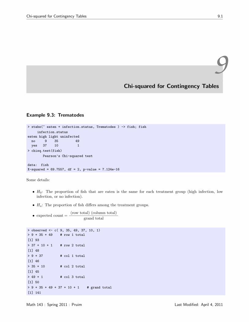
Example 2: Details not in abstract but are in the paper

Abstract

Inheritance of two mutant foliage types, variegatedand purple, was investigated for diploid, triploid, andtetraploid tutsan (Hypericum androsaemum). Thefertility of progeny was evaluated by pollen viabilitytests and reciprocal crosses with diploids, triploids, andtetraploids and germinative capacity of seeds from suc-cessful crosses. Segregation ratios were determined fordiploid crosses in reciprocal di-hybrid F1, F2, BCP1,and BCP2 families and selfed F2s with the parentalphenotypes. F2 tetraploids were derived from inducedautotetraploid F1s. Triploid segregation ratios were de-termined for crosses between tetraploid F2s and diploidF1s. Diploid di-hybrid crosses fit the expected9 : 3 : 3 : 1 ratio for a single, simple recessivegene for both traits, with no evidence of linkage. Anovel phenotype representing a combination of parentalphenotypes was recovered. Data from backcrosses andselfing support the recessive model. Both traits be-haved as expected at the triploid level; however, at thetetraploid level the number of variegated progeny in-creased, with segregation ratios falling between randomchromosome and random chromatid assortment mod-els. We propose the gene symbol var (variegated) andpl (purple leaf) for the variegated and purple genes,respectively. Triploid pollen stained moderately well(41%), but pollen germination was low (6%). Triploidplants were highly infertile, demonstrating extremely

low male fertility and no measurable female fertility (noviable seed production). The present research demon-strates the feasibility of breeding simultaneously for or-namental traits and non-invasiveness.

...

There are many sentences of the following type in thepaper:

And some of the results are summarized in a table.

Source: Richard T. Olsen, Thomas G. Ranney, Dennis J. Werner, J. AMER. SOC. HORT. SCI. 131(6):725–730. 2006. Fertility and Inheritance of Variegated and Purple Foliage Across a Polyploid Series in Hypericumandrosaemum L. http://www.ces.ncsu.edu/fletcher/mcilab/publications/olsen-etal-2006c.pdf


http://www.ces.ncsu.edu/fletcher/mcilab/publications/olsen-etal-2006c.pdf



Chi-squared for Contingency Tables 9.1

9Chi-squared for Contingency Tables

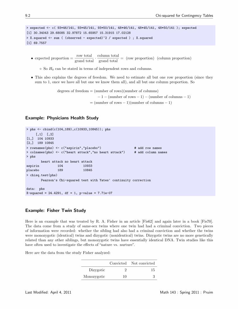
Example 9.3: Trematodes

> xtabs(~ eaten + infection.status, Trematodes ) -> fish; fish

infection.status

eaten high light uninfected

no 9 35 49

yes 37 10 1

> chisq.test(fish)

Pearson's Chi-squared test

data: fish


Some details:

• H0: The proportion of fish that are eaten is the same for each treatment group (high infection, lowinfection, or no infection).

• Ha: The proportion of fish differs among the treatment groups.

• expected count =(row total) (column total)

grand total

> observed <- c( 9, 35, 49, 37, 10, 1)

> 9 + 35 + 49 # row 1 total

[1] 93

> 37 + 10 + 1 # row 2 total

[1] 48

> 9 + 37 # col 1 total

[1] 46

> 35 + 10 # col 2 total

[1] 45

> 49 + 1 # col 3 total

[1] 50

> 9 + 35 + 49 + 37 + 10 + 1 # grand total

[1] 141


9.2 Chi-squared for Contingency Tables

> expected <- c( 93*46/141, 93*45/141, 93*50/141, 48*46/141, 48*45/141, 48*50/141 ); expected

[1] 30.34043 29.68085 32.97872 15.65957 15.31915 17.02128

> X.squared <- sum ( (observed - expected)^2 / expected ) ; X.squared

[1] 69.7557

• expected proportion =row total

grand total· column total

grand total= (row proportion) (column proportion)

◦ So H0 can be stated in terms of independent rows and columns.

• This also explains the degrees of freedom. We need to estimate all but one row proportion (since theysum to 1, once we have all but one we know them all), and all but one column proportion. So

degrees of freedom = (number of rows)(number of columns)

− 1− (number of rows− 1)− (number of columns− 1)

= (number of rows− 1)(number of columns− 1)

Example: Physicians Health Study

> phs <- cbind(c(104,189),c(10933,10845)); phs

[,1] [,2]

[1,] 104 10933

[2,] 189 10845

> rownames(phs) <- c("aspirin","placebo") # add row names

> colnames(phs) <- c("heart attack","no heart attack") # add column names

> phs

heart attack no heart attack

aspirin 104 10933

placebo 189 10845

> chisq.test(phs)

Pearson's Chi-squared test with Yates' continuity correction

data: phs


Example: Fisher Twin Study

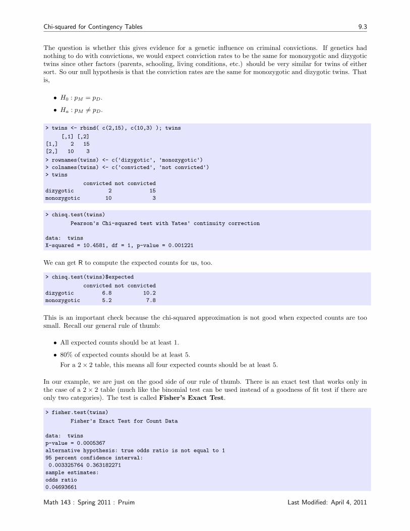
Here is an example that was treated by R. A. Fisher in an article [Fis62] and again later in a book [Fis70].The data come from a study of same-sex twins where one twin had had a criminal conviction. Two piecesof information were recorded: whether the sibling had also had a criminal conviction and whether the twinswere monozygotic (identical) twins and dizygotic (nonidentical) twins. Dizygotic twins are no more geneticallyrelated than any other siblings, but monozygotic twins have essentially identical DNA. Twin studies like thishave often used to investigate the effects of “nature vs. nurture”.

Here are the data from the study Fisher analyzed:

Convicted Not convicted

Dizygotic 2 15

Monozygotic 10 3



The question is whether this gives evidence for a genetic influence on criminal convictions. If genetics hadnothing to do with convictions, we would expect conviction rates to be the same for monozygotic and dizygotictwins since other factors (parents, schooling, living conditions, etc.) should be very similar for twins of eithersort. So our null hypothesis is that the conviction rates are the same for monozygotic and dizygotic twins. Thatis,

• H0 : pM = pD.

• Ha : pM 6= pD.

> twins <- rbind( c(2,15), c(10,3) ); twins

[,1] [,2]

[1,] 2 15

[2,] 10 3

> rownames(twins) <- c('dizygotic', 'monozygotic')> colnames(twins) <- c('convicted', 'not convicted')> twins

convicted not convicted

dizygotic 2 15

monozygotic 10 3

> chisq.test(twins)


data: twins


We can get R to compute the expected counts for us, too.

> chisq.test(twins)$expected

convicted not convicted

dizygotic 6.8 10.2

monozygotic 5.2 7.8

This is an important check because the chi-squared approximation is not good when expected counts are toosmall. Recall our general rule of thumb:

• All expected counts should be at least 1.

• 80% of expected counts should be at least 5.

For a 2× 2 table, this means all four expected counts should be at least 5.

In our example, we are just on the good side of our rule of thumb. There is an exact test that works only inthe case of a 2 × 2 table (much like the binomial test can be used instead of a goodness of fit test if there areonly two categories). The test is called Fisher’s Exact Test.

> fisher.test(twins)

Fisher's Exact Test for Count Data

data: twins

p-value = 0.0005367

alternative hypothesis: true odds ratio is not equal to 1


0.003325764 0.363182271

sample estimates:

odds ratio

0.04693661



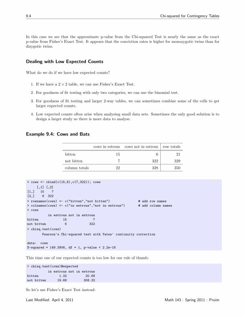
In this case we see that the approximate p-value from the Chi-squared Test is nearly the same as the exactp-value from Fisher’s Exact Test. It appears that the conviction rates is higher for monozygotic twins than fordizygotic twins.

Dealing with Low Expected Counts

What do we do if we have low expected counts?

1. If we have a 2× 2 table, we can use Fisher’s Exact Test.

2. For goodness of fit testing with only two categories, we can use the binomial test.

3. For goodness of fit testing and larger 2-way tables, we can sometimes combine some of the cells to getlarger expected counts.

4. Low expected counts often arise when analysing small data sets. Sometimes the only good solution is todesign a larger study so there is more data to analyse.

Example 9.4: Cows and Bats

cows in estrous cows not in estrous row totals

bitten 15 6 21

not bitten 7 322 329

column totals 22 328 350

> cows <- cbind(c(15,6),c(7,322)); cows

[,1] [,2]

[1,] 15 7

[2,] 6 322

> rownames(cows) <- c("bitten","not bitten") # add row names

> colnames(cows) <- c("in estrous","not in estrous") # add column names

> cows

in estrous not in estrous

bitten 15 7

not bitten 6 322

> chisq.test(cows)


data: cows

X-squared = 149.3906, df = 1, p-value < 2.2e-16

This time one of our expected counts is too low for our rule of thumb:

> chisq.test(cows)$expected

in estrous not in estrous

bitten 1.32 20.68

not bitten 19.68 308.32

So let’s use Fisher’s Exact Test instead:



> fisher.test(cows)

Fisher's Exact Test for Count Data

data: cows

p-value < 2.2e-16

alternative hypothesis: true odds ratio is not equal to 1


29.94742 457.26860

sample estimates:

odds ratio

108.3894

In this example the conclusion is the same: extremely strong evidence against the null hypothesis.

Odds and Odds Ratio

odds = O =p

1− p

=pn

(1− p)n

=number of successes

number of failures

odds ratio = OR =odds1

odds2=

p11−p1p2

1−p2

=p1

1− p1· 1− p2

p2

We can estimate these quantities using data. When we do, we put hats on everything

estimated odds = O =p

1− p

estimated odds ratio = OR =O1

O2

=

p11−p1p2

1−p2

=p1

1− p1· 1− p2

p2

The null hypothesis of Fisher’s Exact Test is that the odds ratio is 1, that is, that the two proportions are equal.fisher.test() uses a somewhat more complicated method to estimate odds ratio, so the formulas above won’texactly match the odds ratio displayed in the output of fisher.test(), but the value will be quite close.

> (2/15) / (10/3) # simple estimate of odds ratio

[1] 0.04

> (10/3) / (2/15) # simple estimate of odds ratio with roles reversed

[1] 25

Notice that when p1 and p1 are small, then 1− p1 and 1− p2 are both close to 1, so

odds ratio ≈ p1

p2= relative risk

Relative risk is easier to understand, but odds ratio has nicer statistical and mathematical properties.




Normal Distributions 10.1

10Normal Distributions

10.1 The Family of Normal Distributions

Normal Distributions

• are symmetric, unimodel, and bell-shaped

• can have any combination of mean and standard deviation (as long as the standard deviation is positive)

• satisfy the 68–95–99.7 rule:

Approximately 68% of any normal distribution lies within 1 standard deviation of the mean.

Approximately 95% of any normal distribution lies within 2 standard deviations of the mean.

Approximately 99.7% of any normal distribution lies within 3 standard deviations of the mean.

standard deviations from the mean

−4 −2 0 2 4

0.683


−4 −2 0 2 4

0.954


−4 −2 0 2 4

0.997

Many naturally occurring distributions are approximately normally distributed.

Normal distributions are also an important part of statistical inference.


10.2 Normal Distributions

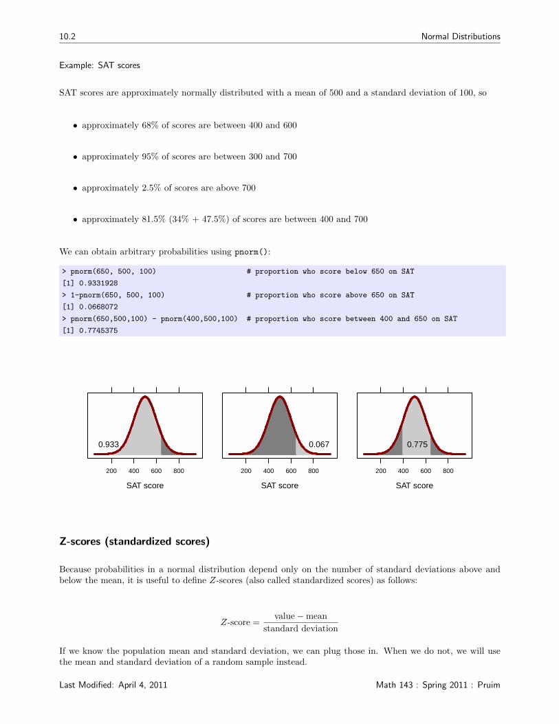
Example: SAT scores

SAT scores are approximately normally distributed with a mean of 500 and a standard deviation of 100, so

• approximately 68% of scores are between 400 and 600

• approximately 95% of scores are between 300 and 700

• approximately 2.5% of scores are above 700

• approximately 81.5% (34% + 47.5%) of scores are between 400 and 700

We can obtain arbitrary probabilities using pnorm():

> pnorm(650, 500, 100) # proportion who score below 650 on SAT

[1] 0.9331928

> 1-pnorm(650, 500, 100) # proportion who score above 650 on SAT

[1] 0.0668072

> pnorm(650,500,100) - pnorm(400,500,100) # proportion who score between 400 and 650 on SAT

[1] 0.7745375

SAT score

200 400 600 800

0.933

SAT score

200 400 600 800

0.067

SAT score

200 400 600 800

0.775

Z-scores (standardized scores)

Because probabilities in a normal distribution depend only on the number of standard deviations above andbelow the mean, it is useful to define Z-scores (also called standardized scores) as follows:

Z-score =value−mean

standard deviation

If we know the population mean and standard deviation, we can plug those in. When we do not, we will usethe mean and standard deviation of a random sample instead.



10.2 The Central Limit Theorem

The importance of the normal distributions comes from the

The Central Limit Theorem. The sampling distribution of a sample mean or sample sum of a largeenough random sample is approximately normally distributed. In fact,

• Y ≈ Norm(µ, σ√n

)

•∑Y ≈ Norm(µ, σ

√n)

The approximations are better

• when the population distribution is similar to a normal distribution,

• when the sample size is larger,

and are exact when the population distribution is normal.

The Central Limit Theorem is illustrated nicely in an applet available from the Rice Virtual Laboratory inStatistics (http://onlinestatbook.com/stat_sim/sampling_dist/index.html).

10.2.1 Normal Approximation to the Binomial

Since a binomial random variable is a sum of 0’s and 1’s from each trial, the Central Limit Theorem impliesthat

Binom(n, p) ≈ Norm(np,√np(1− p)

)Our rule of thumb for the quality of this approximation is that it is good enough for our purposes when np ≥ 5and n(1− p) ≥ 5 – that is, when we would expect at least 5 success and at least 5 failures. (Many books requireat least 10 of each. The true story is that the approximation gets better and better as the smaller of np andn(1− p) gets larger.

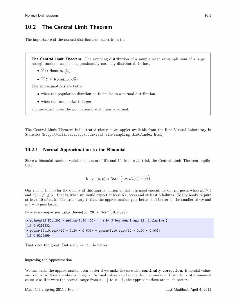
Here is a comparison using Binom(50, .20) ≈ Norm(10, 2.828):

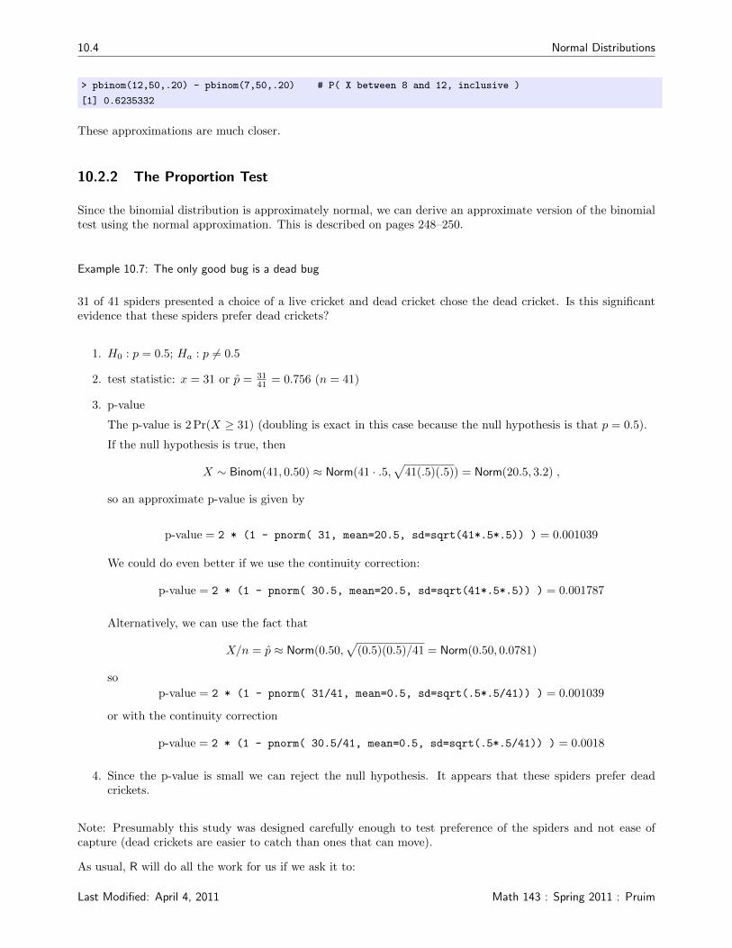
> pbinom(12,50,.20) - pbinom(7,50,.20) # P( X between 8 and 12, inclusive )

[1] 0.6235332

> pnorm(12,10,sqrt(50 * 0.20 * 0.80)) - pnorm(8,10,sqrt(50 * 0.20 * 0.80))

[1] 0.5204999

That’s not too great. But wait, we can do better . . .

Improving the Approximation

We can make the approximation even better if we make the so-called continuity correction. Binomial valuesare counts, so they are always integers. Normal values can be any decimal amount. If we think of a binomialcount x as if it were the normal range from x− 1

2 to x+ 12 , the approximations are much better.


http://onlinestatbook.com/stat_sim/sampling_dist/index.html


> pbinom(12,50,.20) - pbinom(7,50,.20) # P( X between 8 and 12, inclusive )

[1] 0.6235332

These approximations are much closer.

10.2.2 The Proportion Test

Since the binomial distribution is approximately normal, we can derive an approximate version of the binomialtest using the normal approximation. This is described on pages 248–250.

Example 10.7: The only good bug is a dead bug

31 of 41 spiders presented a choice of a live cricket and dead cricket chose the dead cricket. Is this significantevidence that these spiders prefer dead crickets?

1. H0 : p = 0.5; Ha : p 6= 0.5

2. test statistic: x = 31 or p = 3141 = 0.756 (n = 41)

3. p-value

The p-value is 2 Pr(X ≥ 31) (doubling is exact in this case because the null hypothesis is that p = 0.5).

If the null hypothesis is true, then

X ∼ Binom(41, 0.50) ≈ Norm(41 · .5,√

41(.5)(.5)) = Norm(20.5, 3.2) ,

so an approximate p-value is given by

p-value = 2 * (1 - pnorm( 31, mean=20.5, sd=sqrt(41*.5*.5)) ) = 0.001039

We could do even better if we use the continuity correction:

p-value = 2 * (1 - pnorm( 30.5, mean=20.5, sd=sqrt(41*.5*.5)) ) = 0.001787

Alternatively, we can use the fact that

X/n = p ≈ Norm(0.50,√

(0.5)(0.5)/41 = Norm(0.50, 0.0781)

so

p-value = 2 * (1 - pnorm( 31/41, mean=0.5, sd=sqrt(.5*.5/41)) ) = 0.001039

or with the continuity correction

p-value = 2 * (1 - pnorm( 30.5/41, mean=0.5, sd=sqrt(.5*.5/41)) ) = 0.0018

4. Since the p-value is small we can reject the null hypothesis. It appears that these spiders prefer deadcrickets.

Note: Presumably this study was designed carefully enough to test preference of the spiders and not ease ofcapture (dead crickets are easier to catch than ones that can move).

As usual, R will do all the work for us if we ask it to:



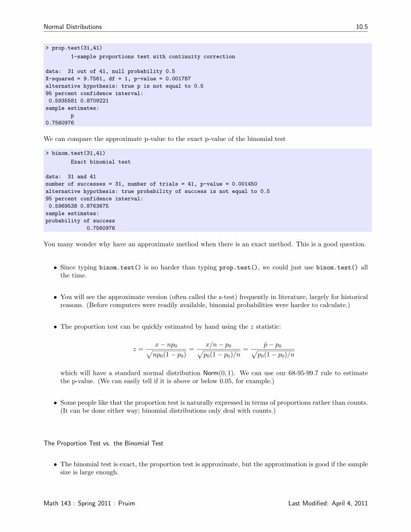
> prop.test(31,41)

1-sample proportions test with continuity correction

data: 31 out of 41, null probability 0.5


alternative hypothesis: true p is not equal to 0.5


0.5935581 0.8709221

sample estimates:

p

0.7560976

We can compare the approximate p-value to the exact p-value of the binomial test

> binom.test(31,41)

Exact binomial test

data: 31 and 41




0.5969538 0.8763675

sample estimates:


0.7560976

You many wonder why have an approximate method when there is an exact method. This is a good question.

• Since typing binom.test() is no harder than typing prop.test(), we could just use binom.test() allthe time.

• You will see the approximate version (often called the z-test) frequently in literature, largely for historicalreasons. (Before computers were readily available, binomial probabilities were harder to calculate.)

• The proportion test can be quickly estimated by hand using the z statistic:

z =x− np0√np0(1− p0)

=x/n− p0√p0(1− p0)/n

=p− p0√

p0(1− p0)/n

which will have a standard normal distribution Norm(0, 1). We can use our 68-95-99.7 rule to estimatethe p-value. (We can easily tell if it is above or below 0.05, for example.)

• Some people like that the proportion test is naturally expressed in terms of proportions rather than counts.(It can be done either way; binomial distributions only deal with counts.)

The Proportion Test vs. the Binomial Test

• The binomial test is exact, the proportion test is approximate, but the approximation is good if the samplesize is large enough.



10.3 Confidence Intervals

Note: Much of this information is from Section 7.3

The sampling distribution for a sample proportion (assuming samples of size n) is

p ∼ Norm

(p,

√p(1− p)

n

)

The standard deviation of a sampling distribution is called the standard error (abbreviated SE), so in this casewe have

SE =

√p(1− p)

n

This means that for 95% of samples, our estimated proportion p will be within (1.96)SE of p. This tells us howwell p approximates p. It says that usually p is between p− 1.96SE and p+ 1.96SE.

Key idea: If p is close to p, then p is close to p.

That is, for most samples p is between p− 1.96SE and p+ 1.96SE.

Our only remaining difficulty is that we don’t know SE because it depends on p, which we don’t know. We willestimate SE as follows.

SE ≈√p(1− p)

n

We will call the interval between p− 1.96√

p(1−p)n and p+ 1.96

√p(1−p)n a 95% confidence interval for p. Often

we will write this very succinctly asp± 1.96SE

(Note: we are being a little bit lazy and using SE for the estimated standard error. Some books only referto these estimates as the standard error, further adding to the notational confusion. Fortunately, the idea issimpler than the notation.)

Example

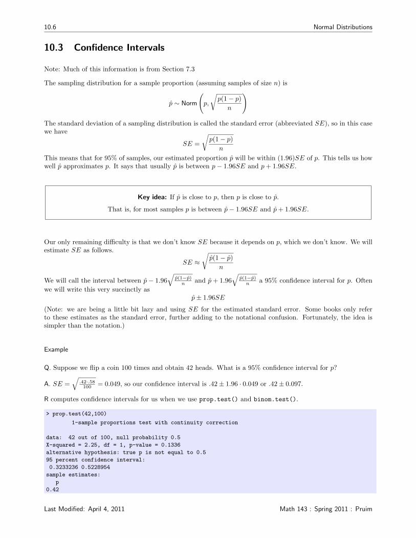
Q. Suppose we flip a coin 100 times and obtain 42 heads. What is a 95% confidence interval for p?

A. SE =√

.42·.58100 = 0.049, so our confidence interval is .42± 1.96 · 0.049 or .42± 0.097.

R computes confidence intervals for us when we use prop.test() and binom.test().

> prop.test(42,100)






0.3233236 0.5228954

sample estimates:

p

0.42



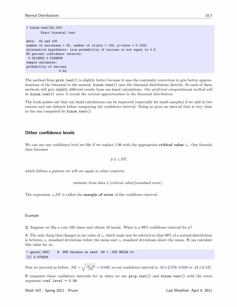
> binom.test(42,100)

Exact binomial test

data: 42 and 100




0.3219855 0.5228808

sample estimates:


0.42

The method from prob.test() is slightly better because it uses the continuity correction to give better approx-imations of the binomial to the normal. binom.test() uses the binomial distribution directly. So each of thesemethods will give slightly different results from our hand calculations. Our preferred computational method willbe binom.test() since it avoids the normal approximation to the binomial distribution.

The book points out that our hand calculations can be improved (especially for small samples) if we add in twosuccess and two failures before computing the confidence interval. Doing so gives an interval that is very closeto the one computed by binom.test().

Other confidence levels

We can use any confidence level we like if we replace 1.96 with the appropriate critical value z∗. Our formulathen becomes

p± z∗SE

which follows a pattern we will see again in other contexts:

estimate from data± (critical value)(standard error) .

The expression z∗SE is called the margin of error of the confidence interval.

Example

Q. Suppose we flip a coin 100 times and obtain 42 heads. What is a 99% confidence interval for p?

A. The only thing that changes is our value of z∗ which must now be selected so that 99% of a normal distributionis between z∗ standard deviations below the mean and z∗ standard deviations above the mean. R can calculatethis value for us:

> qnorm(.995) # .995 because we need .99 + .005 BELOW z*

[1] 2.575829

Now we proceed as before. SE =√

.42·.58100 = 0.049, so our confidence interval is .42±2.576 ·0.049 or .42±0.127.

R computes these confidence intervals for us when we use prop.test() and binom.test() with the extraargument conf.level = 0.99.



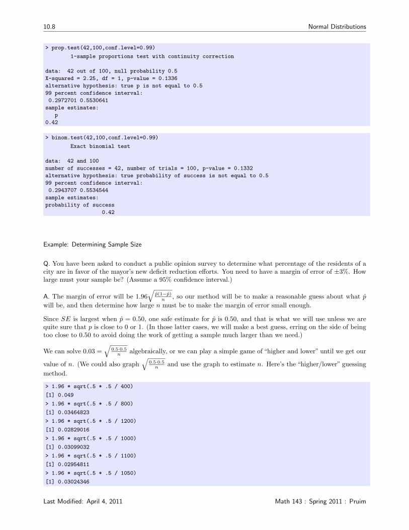
> prop.test(42,100,conf.level=0.99)






0.2972701 0.5530641

sample estimates:

p

0.42

> binom.test(42,100,conf.level=0.99)

Exact binomial test

data: 42 and 100




0.2943707 0.5534544

sample estimates:


0.42

Example: Determining Sample Size

Q. You have been asked to conduct a public opinion survey to determine what percentage of the residents of acity are in favor of the mayor’s new deficit reduction efforts. You need to have a margin of error of ±3%. Howlarge must your sample be? (Assume a 95% confidence interval.)

A. The margin of error will be 1.96√

p(1−p)n , so our method will be to make a reasonable guess about what p

will be, and then determine how large n must be to make the margin of error small enough.

Since SE is largest when p = 0.50, one safe estimate for p is 0.50, and that is what we will use unless we arequite sure that p is close to 0 or 1. (In those latter cases, we will make a best guess, erring on the side of beingtoo close to 0.50 to avoid doing the work of getting a sample much larger than we need.)

We can solve 0.03 =√

0.5·0.5n algebraically, or we can play a simple game of “higher and lower” until we get our

value of n. (We could also graph√

0.5·0.5n and use the graph to estimate n. Here’s the “higher/lower” guessing

method.

> 1.96 * sqrt(.5 * .5 / 400)

[1] 0.049

> 1.96 * sqrt(.5 * .5 / 800)

[1] 0.03464823

> 1.96 * sqrt(.5 * .5 / 1200)

[1] 0.02829016

> 1.96 * sqrt(.5 * .5 / 1000)

[1] 0.03099032

> 1.96 * sqrt(.5 * .5 / 1100)

[1] 0.02954811

> 1.96 * sqrt(.5 * .5 / 1050)

[1] 0.03024346



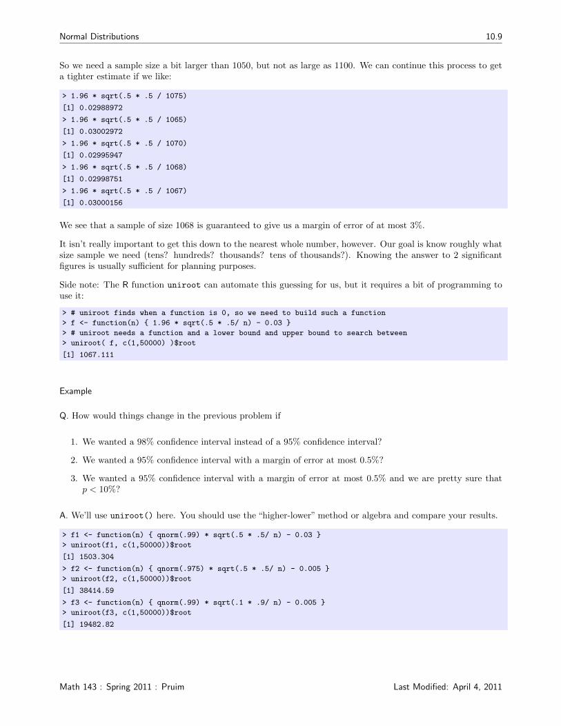
So we need a sample size a bit larger than 1050, but not as large as 1100. We can continue this process to geta tighter estimate if we like:

> 1.96 * sqrt(.5 * .5 / 1075)

[1] 0.02988972

> 1.96 * sqrt(.5 * .5 / 1065)

[1] 0.03002972

> 1.96 * sqrt(.5 * .5 / 1070)

[1] 0.02995947

> 1.96 * sqrt(.5 * .5 / 1068)

[1] 0.02998751

> 1.96 * sqrt(.5 * .5 / 1067)

[1] 0.03000156

We see that a sample of size 1068 is guaranteed to give us a margin of error of at most 3%.

It isn’t really important to get this down to the nearest whole number, however. Our goal is know roughly whatsize sample we need (tens? hundreds? thousands? tens of thousands?). Knowing the answer to 2 significantfigures is usually sufficient for planning purposes.

Side note: The R function uniroot can automate this guessing for us, but it requires a bit of programming touse it:

> # uniroot finds when a function is 0, so we need to build such a function

> f <- function(n) { 1.96 * sqrt(.5 * .5/ n) - 0.03 }

> # uniroot needs a function and a lower bound and upper bound to search between

> uniroot( f, c(1,50000) )$root

[1] 1067.111

Example

Q. How would things change in the previous problem if

1. We wanted a 98% confidence interval instead of a 95% confidence interval?

2. We wanted a 95% confidence interval with a margin of error at most 0.5%?

3. We wanted a 95% confidence interval with a margin of error at most 0.5% and we are pretty sure thatp < 10%?

A. We’ll use uniroot() here. You should use the “higher-lower” method or algebra and compare your results.

> f1 <- function(n) { qnorm(.99) * sqrt(.5 * .5/ n) - 0.03 }

> uniroot(f1, c(1,50000))$root

[1] 1503.304



[1] 38414.59



[1] 19482.82




Inference for the Mean of a Population 11.1

11Inference for the Mean of a Population

The Central Limit Theorem tells us that if we compute the sample mean from a random sample taken from apopulation with mean µ and standard deviation σ, then for large enough samples,

Y ≈ Norm

(µ,

σ√n

)All the results in this section are based on this distribution.

11.1 Hypothesis Tests

11.1.1 T Distributions

The test statistic

z =y − µ0

SE

where

SE =σ√n

has a standard normal distribution, so if we knew σ we would be all set.

Since we don’t know σ we will use the standard deviation of our sample instead:

t =y − µ0

SE

where

SE =s√n.

This does not have a normal distribution, it has a t-distribution with n−1 degrees of freedom. The t-distributionslook like shorter, fatter versions of normal distributions. They become more and more like normal distributionsas the sample size gets larger.

11.1.2 Example: Is the Mean Human Body Temperature Really 98.6?

Let’s answer this question by following or usual 4 step method based on the following sample.


11.2 Inference for the Mean of a Population

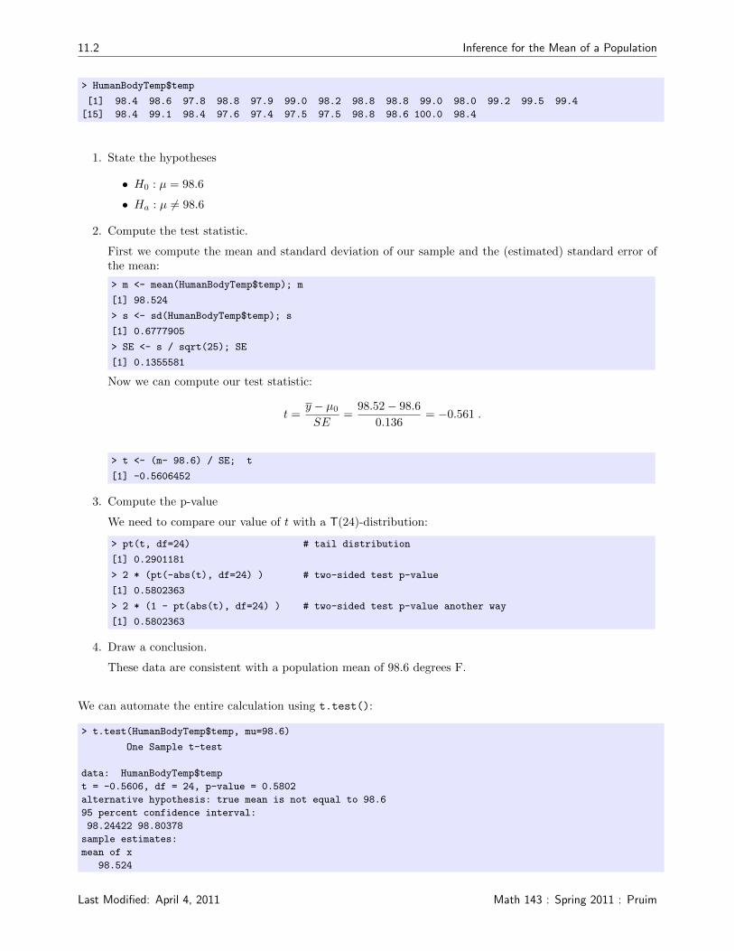
> HumanBodyTemp$temp

[1] 98.4 98.6 97.8 98.8 97.9 99.0 98.2 98.8 98.8 99.0 98.0 99.2 99.5 99.4

[15] 98.4 99.1 98.4 97.6 97.4 97.5 97.5 98.8 98.6 100.0 98.4

1. State the hypotheses

• H0 : µ = 98.6

• Ha : µ 6= 98.6

2. Compute the test statistic.

First we compute the mean and standard deviation of our sample and the (estimated) standard error ofthe mean:

> m <- mean(HumanBodyTemp$temp); m

[1] 98.524

> s <- sd(HumanBodyTemp$temp); s

[1] 0.6777905

> SE <- s / sqrt(25); SE

[1] 0.1355581

Now we can compute our test statistic:

t =y − µ0

SE=

98.52− 98.6

0.136= −0.561 .

> t <- (m- 98.6) / SE; t

[1] -0.5606452

3. Compute the p-value

We need to compare our value of t with a T(24)-distribution:

> pt(t, df=24) # tail distribution

[1] 0.2901181

> 2 * (pt(-abs(t), df=24) ) # two-sided test p-value

[1] 0.5802363

> 2 * (1 - pt(abs(t), df=24) ) # two-sided test p-value another way

[1] 0.5802363

4. Draw a conclusion.

These data are consistent with a population mean of 98.6 degrees F.

We can automate the entire calculation using t.test():

> t.test(HumanBodyTemp$temp, mu=98.6)

One Sample t-test

data: HumanBodyTemp$temp

t = -0.5606, df = 24, p-value = 0.5802

alternative hypothesis: true mean is not equal to 98.6


98.24422 98.80378

sample estimates:

mean of x

98.524


Inference for the Mean of a Population 11.3

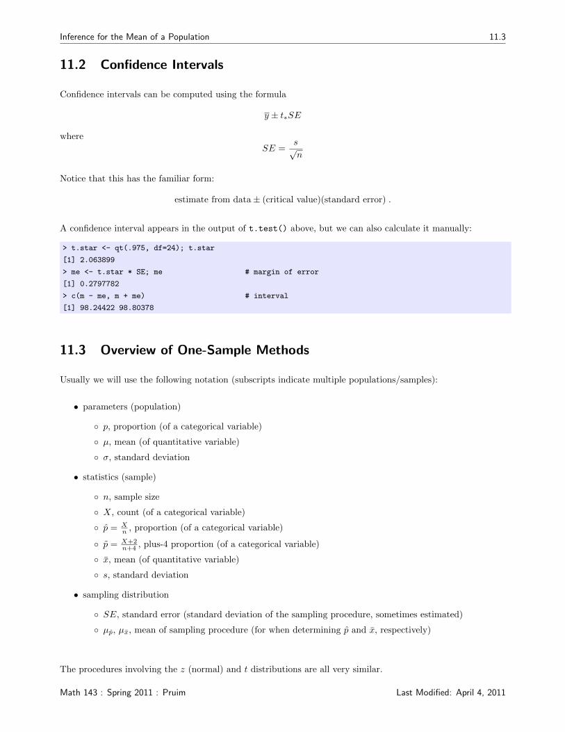
11.2 Confidence Intervals

Confidence intervals can be computed using the formula

y ± t∗SE

where

SE =s√n

Notice that this has the familiar form:

estimate from data± (critical value)(standard error) .

A confidence interval appears in the output of t.test() above, but we can also calculate it manually:

> t.star <- qt(.975, df=24); t.star

[1] 2.063899

> me <- t.star * SE; me # margin of error

[1] 0.2797782

> c(m - me, m + me) # interval

[1] 98.24422 98.80378

11.3 Overview of One-Sample Methods

Usually we will use the following notation (subscripts indicate multiple populations/samples):

• parameters (population)

◦ p, proportion (of a categorical variable)

◦ µ, mean (of quantitative variable)

◦ σ, standard deviation

• statistics (sample)

◦ n, sample size

◦ X, count (of a categorical variable)

◦ p = Xn , proportion (of a categorical variable)

◦ p = X+2n+4 , plus-4 proportion (of a categorical variable)

◦ x, mean (of quantitative variable)

◦ s, standard deviation

• sampling distribution

◦ SE, standard error (standard deviation of the sampling procedure, sometimes estimated)

◦ µp, µx, mean of sampling procedure (for when determining p and x, respectively)

The procedures involving the z (normal) and t distributions are all very similar.


11.4 Inference for the Mean of a Population

• To do a hypothesis test, compute the test statistic as

t or z =data value− hypothesis value

SE,

and compare with the appropriate distribution (using tables or a computer).

• To compute a confidence interval, determine the critical value for the desired level of confidence (z∗ ort∗), then the confidence interval is

data value± (critical value)(SE) .

Note: Each of these procedures is only valid when certain assumptions are met. In particular, remember

• The sample must be an SRS (or something very close to it).

• The sample sizes must be “large enough.”

• Procedures involving means are generally sensitive to outliers, because outliers can have a large effect onthe mean (and standard deviation).

• Procedures involving the t statistic generally assume a population that is normal or nearly normal. Theseprocedures are sensitive to to skewness (for small sample sizes) and to outliers (for any size).

• You can’t do good statistics from bad data. The margin of error in a confidence interval, for example,only accounts for random sampling errors, not for errors in experimental design.


Comparing Two Means 12.1

12Comparing Two Means

12.1 The Distinction Between Paired T and 2-sample T

• A paired t-test or interval compares two quantitative variables measure on the same observational units.

◦ Data: two quantitative variables

◦ Example: each swimmer swims in both water and syrup and we compare the speeds. We recordspeed in water (quantitative) and speed in syrup (quantitative) for each swimmer.

• A paired t-test is really just a 1-sample t-test after we take our two measurements and combine them intoone, typically by taking the difference (most common) or the ratio.

• A 2-sample t-test or interval looks at one quantitative variable in two populations.

◦ Data: one quantitative variable and one categorical variable (telling which group the subject is in).

◦ Example: Some swimmers swim in water, some swim in syrup. We record the speed (quantitative)and what they swam in (categorical) for each swimmer.

An advantage of the paired design (when it is available) is the potential to reduce the amount of variability bycomparing individuals to themselves rather than comparing individuals to individuals in an independent sample.

Paired tests can also be used for “matched pairs designs” where the observational units are pairs of people,animals, etc. For example, we could use a matched pairs design with married couples as observational units.We would have one quantitative variable for the husband and one for the wife.

In a 2-sample situation, we need two independent samples (or as close as we can get to that).


12.2 Comparing Two Means

12.2 Comparing Two Means in R

12.2.1 Using R for Paired T

> react <- read.csv('http://www.calvin.edu/~rpruim/data/calvin/react.csv')> # Is there improvement from first try to second try with the dominant hand?

> t.test(react$dom1 - react$dom2)

One Sample t-test

data: react$dom1 - react$dom2

t = -1.6024, df = 19, p-value = 0.1256

alternative hypothesis: true mean is not equal to 0


-2.3062108 0.3062108

sample estimates:

mean of x

-1

> # This gives slightly nicer labeling of the otherwise identical output

> t.test(react$dom1, react$dom2, paired=TRUE)

Paired t-test

data: react$dom1 and react$dom2

t = -1.6024, df = 19, p-value = 0.1256

alternative hypothesis: true difference in means is not equal to 0


-2.3062108 0.3062108

sample estimates:

mean of the differences

-1

12.2.2 Using R for 2-Sample T

> # Is there improvement from first try to second try?

> t.test(dom1 ~ Sex.of.Subject, react)

Welch Two Sample t-test

data: dom1 by Sex.of.Subject

t = -0.5098, df = 17.998, p-value = 0.6164



-4.096683 2.496683

sample estimates:

mean in group female mean in group male

30.0 30.8

> # Is the first try with the dominant hand better if you get to do the other hand first?

> t.test(dom1 ~ Hand.Pattern, react)

Welch Two Sample t-test

data: dom1 by Hand.Pattern

t = -1.0936, df = 16.521, p-value = 0.2898



-4.642056 1.477221

sample estimates:

mean in group dominant first mean in group other first

29.84615 31.42857


Comparing Two Means 12.3

12.3 Formulas for 2-Sample T


12.4 Comparing Two Means


Bibliography

[Fis62] R. A. Fisher, Confidence limits for a cross-product ratio, Australian Journal of Statistics 4 (1962).

[Fis70] , Statistical methods for research workers, 14th ed., Oliver & Boyd, 1970.

5

Date post:	13-Jun-2018
Category:	Documents
Upload:	duongthuy
View:	214 times
Download:	0 times

Math 143: Introduction to Biostatisticsrpruim/courses/m143/S11/fromClass/Math143S...X-squared =...

Documents