Math 413: Introduction to Analysisepearse/resources/Math413-AdvAnalysis/lecture... · 3.3.1 Key...

Math 413: Introduction to Analysis

Erin P. J. Pearse

May 2, 2007

2 Math 413

Contents

0 Pre-preliminaries 7

0.1 Course Overview . . . . . . . . . . . . . . . . . . . . . . . . . . . . . . . . . 7

0.2 Logic and inference . . . . . . . . . . . . . . . . . . . . . . . . . . . . . . . . 8

0.2.1 Set operations and logical connectives. . . . . . . . . . . . . . . . . . 13

1 Preliminaries 15

1.1 Quantifiers . . . . . . . . . . . . . . . . . . . . . . . . . . . . . . . . . . . . 15

1.2 Infinite Sets . . . . . . . . . . . . . . . . . . . . . . . . . . . . . . . . . . . . 18

1.2.1 Countable sets . . . . . . . . . . . . . . . . . . . . . . . . . . . . . . 18

1.3 The rational numbers . . . . . . . . . . . . . . . . . . . . . . . . . . . . . . 22

1.3.1 The abstract structure of Q. . . . . . . . . . . . . . . . . . . . . . . . 22

1.4 Axiom of Choice . . . . . . . . . . . . . . . . . . . . . . . . . . . . . . . . . 26

1.5 A vocabulary for sequences . . . . . . . . . . . . . . . . . . . . . . . . . . . 27

2 Construction of the real numbers 29

2.1 Cauchy sequences . . . . . . . . . . . . . . . . . . . . . . . . . . . . . . . . . 30

2.2 The reals as an ordered field . . . . . . . . . . . . . . . . . . . . . . . . . . . 33

2.3 Limits and completeness . . . . . . . . . . . . . . . . . . . . . . . . . . . . . 35

2.4 Other constructions . . . . . . . . . . . . . . . . . . . . . . . . . . . . . . . 37

3 Topology of the Real Line 39

3.1 Limits and bounds . . . . . . . . . . . . . . . . . . . . . . . . . . . . . . . . 39

3.1.1 Limit Points . . . . . . . . . . . . . . . . . . . . . . . . . . . . . . . 42

3.2 Open sets and closed sets . . . . . . . . . . . . . . . . . . . . . . . . . . . . 47

3.2.1 Open sets . . . . . . . . . . . . . . . . . . . . . . . . . . . . . . . . . 47

3.3 Compact sets . . . . . . . . . . . . . . . . . . . . . . . . . . . . . . . . . . . 53

4 Math 413 CONTENTS

3.3.1 Key properties of compactness . . . . . . . . . . . . . . . . . . . . . 57

4 Continuous functions 59

4.1 Concepts of continuity . . . . . . . . . . . . . . . . . . . . . . . . . . . . . . 59

4.1.1 Definitions . . . . . . . . . . . . . . . . . . . . . . . . . . . . . . . . 59

4.1.2 Limits of functions and limits of sequences . . . . . . . . . . . . . . . 61

4.1.3 Inverse images of open sets . . . . . . . . . . . . . . . . . . . . . . . 62

4.1.4 Related definitions . . . . . . . . . . . . . . . . . . . . . . . . . . . . 63

4.2 Properties of continuity . . . . . . . . . . . . . . . . . . . . . . . . . . . . . 65

5 Differentiation 71

5.1 Concepts of the derivative . . . . . . . . . . . . . . . . . . . . . . . . . . . . 71

5.1.1 Definitions . . . . . . . . . . . . . . . . . . . . . . . . . . . . . . . . 71

5.1.2 Continuity and differentiability . . . . . . . . . . . . . . . . . . . . . 72

5.2 Properties of the derivative . . . . . . . . . . . . . . . . . . . . . . . . . . . 73

5.2.1 Local properties . . . . . . . . . . . . . . . . . . . . . . . . . . . . . 73

5.2.2 IVT and MVT . . . . . . . . . . . . . . . . . . . . . . . . . . . . . . 73

5.3 Calculus of derivatives . . . . . . . . . . . . . . . . . . . . . . . . . . . . . . 76

5.3.1 Arithmetic rules . . . . . . . . . . . . . . . . . . . . . . . . . . . . . 76

5.4 Higher derivatives and Taylor’s Thm . . . . . . . . . . . . . . . . . . . . . . 78

5.4.1 Interpretations of f ′′ . . . . . . . . . . . . . . . . . . . . . . . . . . . 78

5.4.2 Taylor’s Thm . . . . . . . . . . . . . . . . . . . . . . . . . . . . . . . 78

6 Integration 81

6.1 Integrals of continuous functions . . . . . . . . . . . . . . . . . . . . . . . . 81

6.1.1 Existence of the integral . . . . . . . . . . . . . . . . . . . . . . . . . 81

6.2 Properties of the Riemann Integral . . . . . . . . . . . . . . . . . . . . . . . 86

6.3 Improper Integrals . . . . . . . . . . . . . . . . . . . . . . . . . . . . . . . . 91

7 Sequences and Series of Functions 93

7.1 Complex Numbers . . . . . . . . . . . . . . . . . . . . . . . . . . . . . . . . 93

7.1.1 Basic properties of C . . . . . . . . . . . . . . . . . . . . . . . . . . . 93

7.2 Numerical Series and Sequences . . . . . . . . . . . . . . . . . . . . . . . . . 97

7.2.1 Convergence and absolute convergence . . . . . . . . . . . . . . . . . 97

7.2.2 Rearrangements . . . . . . . . . . . . . . . . . . . . . . . . . . . . . 104

7.2.3 Summation by parts . . . . . . . . . . . . . . . . . . . . . . . . . . . 105

CONTENTS 5

7.3 Uniform convergence . . . . . . . . . . . . . . . . . . . . . . . . . . . . . . . 108

7.3.1 Definition of uniform convergence . . . . . . . . . . . . . . . . . . . . 110

7.3.2 Criteria for uniform convergence . . . . . . . . . . . . . . . . . . . . 111

7.3.3 Continuity and uniform convergence . . . . . . . . . . . . . . . . . . 111

7.3.4 Spaces of functions . . . . . . . . . . . . . . . . . . . . . . . . . . . . 113

7.3.5 Term-by-term integration . . . . . . . . . . . . . . . . . . . . . . . . 114

7.3.6 Term-by-term differentiation . . . . . . . . . . . . . . . . . . . . . . 115

7.4 Power series . . . . . . . . . . . . . . . . . . . . . . . . . . . . . . . . . . . . 117

7.4.1 Radius of convergence . . . . . . . . . . . . . . . . . . . . . . . . . . 117

7.4.2 Analytic continuation . . . . . . . . . . . . . . . . . . . . . . . . . . 118

7.5 Approximation by polynomials . . . . . . . . . . . . . . . . . . . . . . . . . 120

7.5.1 Convolution and approximate identities . . . . . . . . . . . . . . . . 120

7.5.2 The Stone-Weierstrass Theorem . . . . . . . . . . . . . . . . . . . . 125

7.5.3 Convolution and differential equations . . . . . . . . . . . . . . . . . 128

6 Math 413 CONTENTS

Chapter 0

Pre-preliminaries

0.1 Course Overview

The study of the real numbers, R, and functions of a real var, f(x) = y where x, y real.

Given f : R→ R which describes some system, how to study f?

• Need rigourous vocab for properties of f (definitions)

• Need to see when some properties imply others (theorems)

Result: can make inferences about the system.

Motivation for analysis: limits, the heart & soul of calculus.

Limits provide a rigourous basis for ideas like sequences, series, continuity, derivatives,

integrals. More adv: model an arbitrary function as a limit of a sequence of “nice”

functions (polys, trigs) or as a sum of “nice” functions (Fourier, wavelets). All of this

requires understanding limits of numbers.

Outline:

1. Logic: not, and, or, implication; rules of inference

2. Sets: elements, intersection, union, containment; special sets

3. The real numbers: algebraic properties (+,×), order properties (<), completeness

properties

8 Math 413 Pre-preliminaries

4. Sequences: types of, convergence, basic results (arithmetic, etc), subsequences, con-

vergence, Cauchy sequences

5. Series: convergence tests, absolute convergence, power series

6. Functions: arith, behavior, continuity & limits, IVT, compact domains

7. Differentiation: MVT, L’Hopital, Taylor & linearization

8. Integrals: integrability and the Riemann integral

9. Special functions: exp, log, gamma

10. Seqs and series of functions

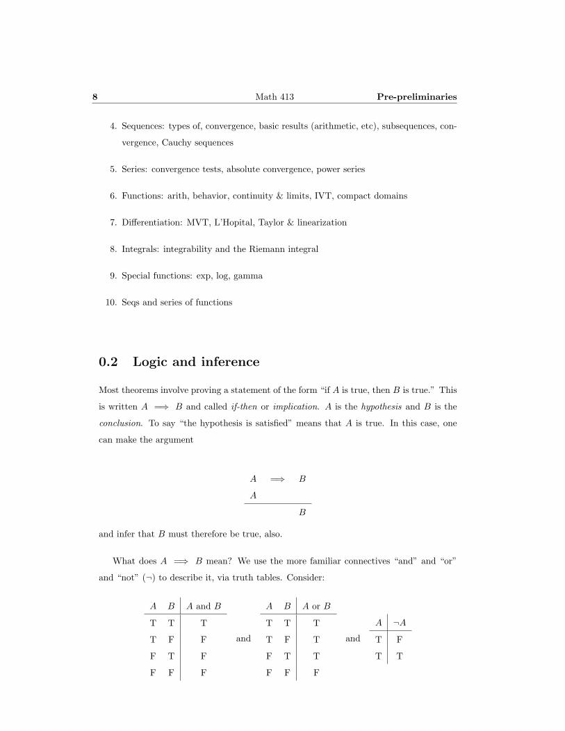
0.2 Logic and inference

Most theorems involve proving a statement of the form “if A is true, then B is true.” This

is written A =⇒ B and called if-then or implication. A is the hypothesis and B is the

conclusion. To say “the hypothesis is satisfied” means that A is true. In this case, one

can make the argument

A =⇒ B

A

B

and infer that B must therefore be true, also.

What does A =⇒ B mean? We use the more familiar connectives “and” and “or”

and “not” (¬) to describe it, via truth tables. Consider:

A B A and B

T T T

T F F

F T F

F F F

and

A B A or B

T T T

T F T

F T T

F F F

and

A ¬A

T F

T T

0.2 Logic and inference 9

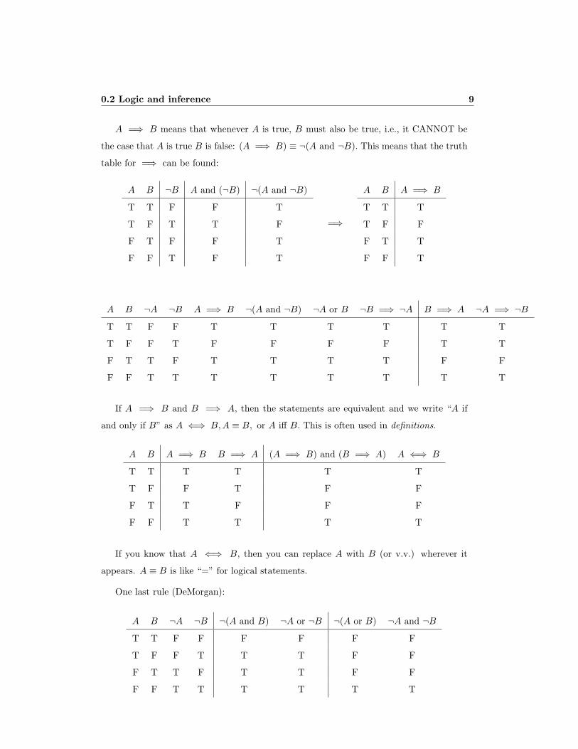
A =⇒ B means that whenever A is true, B must also be true, i.e., it CANNOT be

the case that A is true B is false: (A =⇒ B) ≡ ¬(A and ¬B). This means that the truth

table for =⇒ can be found:

A B ¬B A and (¬B) ¬(A and ¬B)

T T F F T

T F T T F

F T F F T

F F T F T

=⇒

A B A =⇒ B

T T T

T F F

F T T

F F T

A B ¬A ¬B A =⇒ B ¬(A and ¬B) ¬A or B ¬B =⇒ ¬A B =⇒ A ¬A =⇒ ¬B

T T F F T T T T T T

T F F T F F F F T T

F T T F T T T T F F

F F T T T T T T T T

If A =⇒ B and B =⇒ A, then the statements are equivalent and we write “A if

and only if B” as A ⇐⇒ B,A ≡ B, or A iff B. This is often used in definitions.

A B A =⇒ B B =⇒ A (A =⇒ B) and (B =⇒ A) A ⇐⇒ B

T T T T T T

T F F T F F

F T T F F F

F F T T T T

If you know that A ⇐⇒ B, then you can replace A with B (or v.v.) wherever it

appears. A ≡ B is like “=” for logical statements.

One last rule (DeMorgan):

A B ¬A ¬B ¬(A and B) ¬A or ¬B ¬(A or B) ¬A and ¬B

T T F F F F F F

T F F T T T F F

F T T F T T F F

F F T T T T T T


Thus, ¬(A and B) ≡ (¬A or ¬B) and ¬(A or B) ≡ (¬A and ¬B).

Example 0.2.1. Thm: a bounded increasing sequence converges.

This means: If a sequence {an} is increasing and bounded, then it converges, i.e.,

({an} increasing) and ({an} bounded) =⇒ {an} converges.

Suppose we are considering the sequence where an = 1 − 1n . We apply the theorem and

see that an must converge (to something?).

Suppose we are considering the sequence an = (−1)n, which is known to diverge. The

theorem is still helpful; by contrapositive,

¬({an} converges) =⇒ ¬(({an} increasing) and ({an} bounded))

{an} diverges =⇒ ¬({an} increasing) or ¬({an} bounded),

using DeMorgan. So an is either not increasing or unbounded. However, an is bounded,

because every term is contained in the finite interval [−1, 1]. Thus, we can infer that an

must not be increasing. (Note: not increasing does not imply decreasing!)

How to prove A =⇒ B.

Direct proof.

1. Assume the hypothesis, i.e., assume A is true, just for now.

2. Apply this “fact” and other basic knowledge.

3. Show that B is true, based on all this.

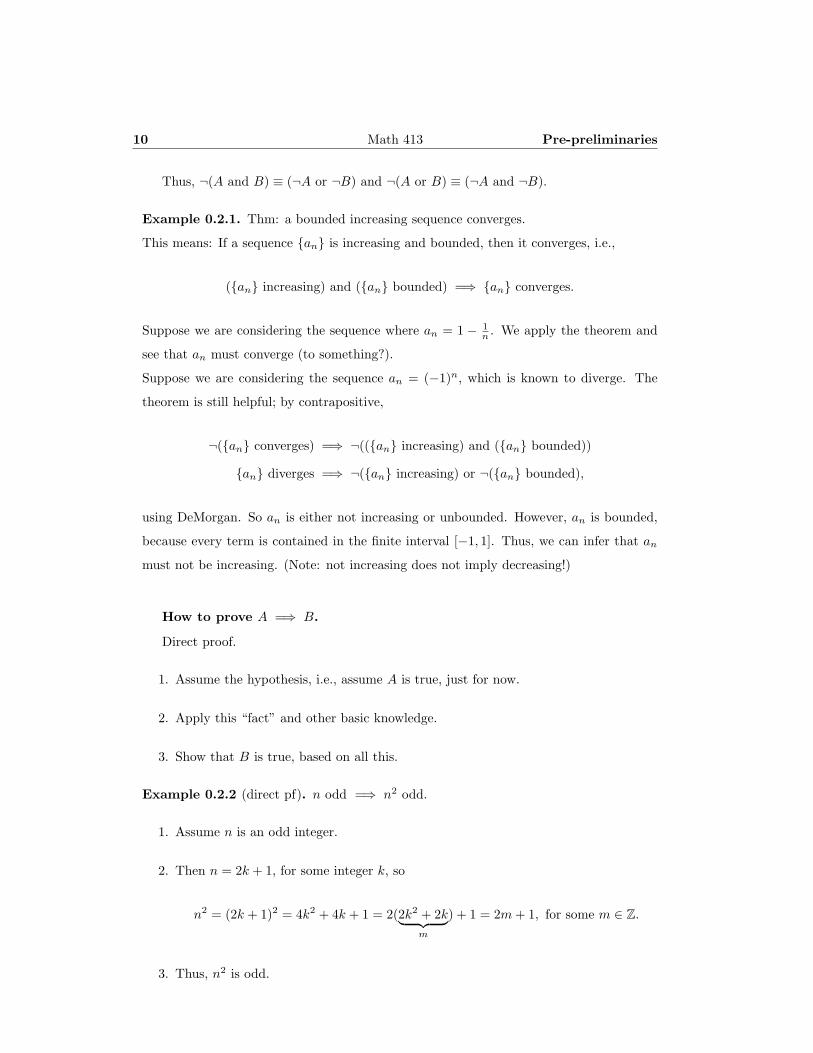
Example 0.2.2 (direct pf). n odd =⇒ n2 odd.

1. Assume n is an odd integer.

2. Then n = 2k + 1, for some integer k, so

n2 = (2k + 1)2 = 4k2 + 4k + 1 = 2(2k2 + 2k︸︷︷︸m

) + 1 = 2m + 1, for some m ∈ Z.

3. Thus, n2 is odd.


Indirect proof: Proof by contrapositive.

(A =⇒ B) ≡ (¬B =⇒ ¬A),

so show ¬B =⇒ ¬A directly.

Example 0.2.3 (contrapositive). 3n + 2 odd =⇒ n odd.

The contrapositive is: n even =⇒ 3n + 2 even.

1. Assume n is an even integer.

2. Then n = 2k, for some integer k, so

3n + 2 = 3(2k) + 2 = 6k + 2 = 2(3k + 1) = 2m, for some m ∈ Z.

3. Thus, 3n + 2 is even.

Example 0.2.4 (contrapositive). n2 even =⇒ n even.

This is just the contrapositive of the prev. example.

Indirect proof: Proof by contradiction.

In order to show that A is true by contradiction,

1. assume that A is false (assume ¬A is true)

2. derive a contradiction (show that ¬A implies something which is clearly false/impossible)

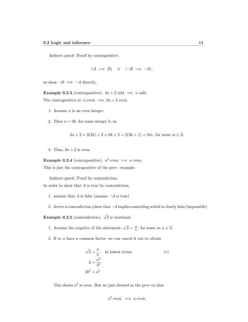
Example 0.2.5 (contradiction).√

2 is irrational.

1. Assume the negative of the statement:√

2 = mn , for some m,n ∈ Z.

2. If m,n have a common factor, we can cancel it out to obtain

√2 =

a

b, in lowest terms (∗)

2 =a2

b2

2b2 = a2

This shows a2 is even. But we just showed in the prev ex that

a2 even =⇒ a even,


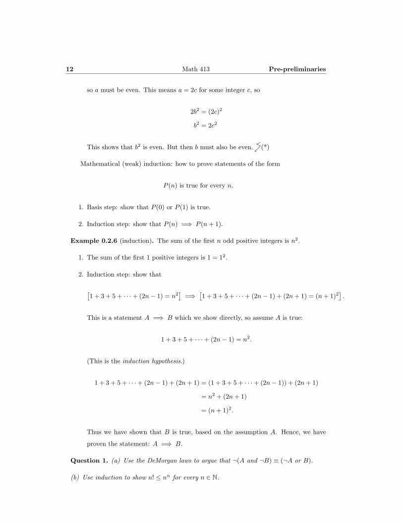
so a must be even. This means a = 2c for some integer c, so

2b2 = (2c)2

b2 = 2c2

This shows that b2 is even. But then b must also be even. <↙(*)

Mathematical (weak) induction: how to prove statements of the form

P (n) is true for every n.

1. Basis step: show that P (0) or P (1) is true.

2. Induction step: show that P (n) =⇒ P (n + 1).

Example 0.2.6 (induction). The sum of the first n odd positive integers is n2.

1. The sum of the first 1 positive integers is 1 = 12.

2. Induction step: show that

[1 + 3 + 5 + · · ·+ (2n− 1) = n2

]=⇒ [

1 + 3 + 5 + · · ·+ (2n− 1) + (2n + 1) = (n + 1)2].

This is a statement A =⇒ B which we show directly, so assume A is true:

1 + 3 + 5 + · · ·+ (2n− 1) = n2.

(This is the induction hypothesis.)

1 + 3 + 5 + · · ·+ (2n− 1) + (2n + 1) = (1 + 3 + 5 + · · ·+ (2n− 1)) + (2n + 1)

= n2 + (2n + 1)

= (n + 1)2.

Thus we have shown that B is true, based on the assumption A. Hence, we have

proven the statement: A =⇒ B.

Question 1. (a) Use the DeMorgan laws to argue that ¬(A and ¬B) ≡ (¬A or B).

(b) Use induction to show n! ≤ nn for every n ∈ N.


0.2.1 Set operations and logical connectives.

intersection: A ∩B = {x ... x ∈ A and x ∈ B}

union: A ∪B = {x ... x ∈ A or x ∈ B}

complement: Ac = {x ... x /∈ A}

difference: A \B = {x ... x ∈ A and x /∈ B} = A ∩Bc

product: A×B = {(x, y) ... x ∈ A and y ∈ B}

containment: A ⊆ B ⇐⇒ (x ∈ A =⇒ x ∈ B)

Example 0.2.7. “Convergent sequences are bounded.”

({an} is convergent) =⇒ ({an} is bounded)

The set of convergent sequences is a subset of the bounded sequences.

Question 2. (a) Use the DeMorgan laws to argue that (A∩B)c = Ac∪Bc and (A∪B)c =

Ac ∩Bc.

(b) Prove that the empty set is a subset of every set.


Chapter 1

Preliminaries

1.1 Quantifiers

1

Sentential logic/propositional calculus:

A,B are absolute statements about the state of affairs. Any expression like A is (globally)

true or false.

How to express more delicate ideas: relations between specific objects/individuals, etc?

Predicate logic (aka 1st order logic):

A(x), B(x) are statements about a variable x. It may be that A(n) is true but A(m) is

false!

So how to express when something is always true or sometimes true or never true?

Use quantifiers.

Definition 1.1.1 (Universal quantifier). If A(x) is true for every possible value of x

(under discussion), we say ∀x,A(x).

Example 1.1.1. x2 ≥ 0, ∀x ∈ R. TRUE

∀x, a < b =⇒ a2 < b2. FALSE

∀x ≥ 0, a < b =⇒ a2 < b2. TRUE

∀x ∈ (0, 1), ∀n, xn < x. TRUE (assume n ∈ N).

1May 2, 2007

16 Math 413 Preliminaries

Definition 1.1.2 (Existential quantifier). If A(x) is true for at least one allowable value

of x, we say ∃x,A(x), or ∃x such that A(x).

Example 1.1.2. ∃x, x = −x. TRUE (x = 0)

∃x, x2 = x. TRUE (x = 0, 1)

What are the negations?

¬∃x,A(x) means there is no x for which A(x) is true, i.e., A(x) is false for every x:

¬∃x,A(x) ≡ ∀x,¬A(x).

∃x,¬A(x) means there is an x for which A(x) is false, i.e., A(x) is not true for every x:

∃x,¬A(x) ≡ ¬∀x,A(x).

Example 1.1.3. 1. ¬∃x ∈ R, x2 < 0 is the same as ∀x ∈ R, x2 ≥ 0.

2. Not every triangle is equilateral: ¬∀t, Eq(t).

There are nonequilateral triangles: ∃t,¬Eq(t).

3. Every prime number is odd:

∀p ∈ P, Odd(p) ⇐⇒ ¬¬∀p ∈ P, Odd(p) ⇐⇒ ¬∃p ∈ P,¬Odd(p).

We used A ≡ ¬¬A. However, 2 ∈ P and ¬Odd(2) imply the contradiction ∃p,¬Odd(p).

Therefore, the original statement ∀p ∈ P, Odd(p) is false.

Order of quantifiers.

∀x, ∀y, A(x, y) ≡ ∀y, ∀x,A(x, y)

∃x, ∃y, A(x, y) ≡ ∃y, ∃x,A(x, y)

However, cannot interchange different types of quantifier!

∃x, ∀y, A(x, y) ≡/ ∀y, ∃x,A(x, y)

Example 1.1.4. Suppose M(x, y) means “x is the mother of y”. Then:

∀y, ∃x,M(x, y) means that every y has a mother, but

∃x, ∀y, M(x, y) means that there is some x which is the mother of every y.

1.1 Quantifiers 17

Note: one implication is valid.

∃x, ∀y, A(x, y) =⇒ ∀y, ∃x,A(x, y).

1.1.3 Exercises: #3 Due: Jan. 29

Question 3. Interpret in words: ∀x, ∃y, y > x but not ∃y, ∀x, y > x. (x, y are integers)


1.2 Infinite Sets

1.2.1 Countable sets

Definition 1.2.1. Two sets A and B have the same cardinality iff they can be put in

one-to-one correspondence, i.e., if every element of A corresponds to a unique element of

B; all elements are “paired off”.

Cardinality is “size” for finite sets, but it works for infinite sets, too.

Definition 1.2.2. A set A is infinite iff there is a proper subset B ⊆ A which has the

same cardinality as A.

Definition 1.2.3. A set A is countable iff it has the same cardinality as the natural

numbers N = {1, 2, 3, 4, . . . }, i.e., if we can write

A = {a1, a2, a3, . . . }.

Are some infinite sets larger than others? Yes! Some sets have too many elements to

count.

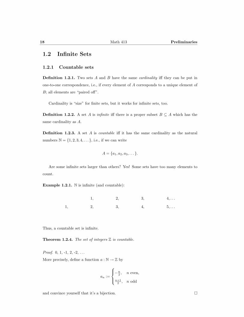
Example 1.2.1. N is infinite (and countable):

1, 2, 3, 4, . . .

1, 2, 3, 4, 5, . . .

Thus, a countable set is infinite.

Theorem 1.2.4. The set of integers Z is countable.

Proof. 0, 1, -1, 2, -2, . . .

More precisely, define a function a : N→ Z by

an :=

−n

2 , n even,

n+12 , n odd

and convince yourself that it’s a bijection.

1.2 Infinite Sets 19

Theorem 1.2.5. N is “the smallest” infinite set, i.e., every subset of N is either finite or

countable.

Proof. Homework. Write it out, cross ’em off.

Theorem 1.2.6. If A is countable and B is countable, then A ∪B is countable.

Proof. Since A = {a1, a2, a3, . . . } and B = {b1, b2, b3, . . . }, we can write

A ∪B = {a1, b1, a2, b2, a3, b3, . . . }.

That was a direct proof.

Theorem 1.2.7. Suppose A1, A2, A3, . . . An are countable. Then the union is also count-

able:n⋃

k=1

Ak = A1 ∪ · · · ∪An = {x ... x ∈ Ak, for some n}.

Proof. Homework. Use induction and the previous result.

What if we take an infinite union?

Theorem 1.2.8. Suppose A1, A2, A3, . . . is a countable sequence of countable sets. Then

the union is also countable:

∞⋃

k=1

Ak = {x ... ∃k such that x ∈ Ak}.

Proof. If we write Ai = {ai1, ai,2, . . . }, then: (grid).

How about a product?

Theorem 1.2.9. Suppose A1, A2, A3, . . . An are countable. Then so is the product:

n∏

k=1

Ak = A1 ×A2 ×A3 × · · · ×An = {(a1, a2, . . . , an) ... ak ∈ Ak}

Proof. We use induction. The basis step is to see that the product of two countable sets

is countable:

A×B = {(x, y) ... x ∈ A, y ∈ B} =

⋃

x∈A

⋃

y∈B

(x, y).


Now for the induction step, assume∏n−1

k=1 Ak is countable. Then

A1 ×A2 ×A3 × · · · ×An−1 ×An =

(n−1∏

k=1

Ak

)×An

is a product of two countable sets, hence countable by the basis step.

Corollary 1.2.10. The set of rational numbers Q is countable.

Proof. Homework.

How about a countable product?

Theorem 1.2.11. Let A1, A2, A3, . . . all have more than one element. Then∏∞

k=1 Ak is

uncountable.

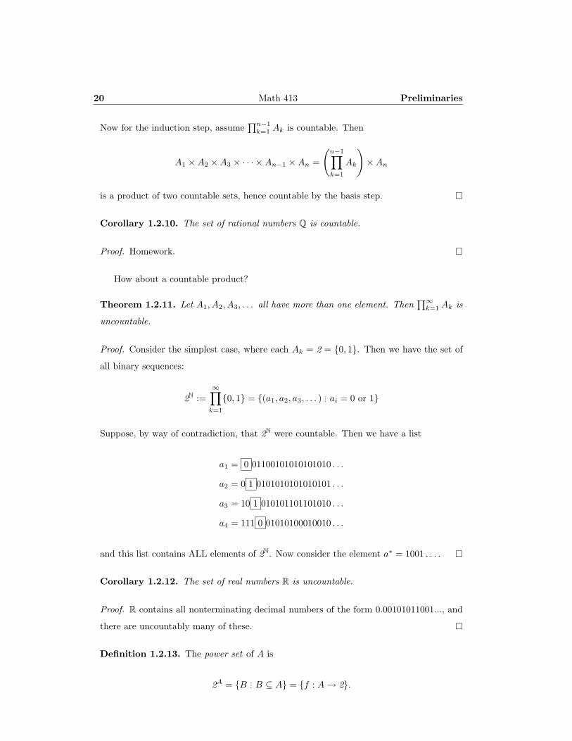
Proof. Consider the simplest case, where each Ak = 2 = {0, 1}. Then we have the set of

all binary sequences:

2N :=∞∏

k=1

{0, 1} = {(a1, a2, a3, . . . ) ... ai = 0 or 1}

Suppose, by way of contradiction, that 2N were countable. Then we have a list

a1 = 0 01100101010101010 . . .

a2 = 0 1 0101010101010101 . . .

a3 = 10 1 010101101101010 . . .

a4 = 111 0 01010100010010 . . .

and this list contains ALL elements of 2N. Now consider the element a∗ = 1001 . . . .

Corollary 1.2.12. The set of real numbers R is uncountable.

Proof. R contains all nonterminating decimal numbers of the form 0.00101011001..., and

there are uncountably many of these.

Definition 1.2.13. The power set of A is

2A = {B ... B ⊆ A} = {f : A → 2}.

1.2 Infinite Sets 21

Example 1.2.2. Suppose A = {1, 2, 3, 4, 5}. Then the subset {2, 3, 5} corresponds to

(0, 1, 1, 0, 1) ∈ 2A. This is the function 1 7→ 0, 2 7→ 1, 3 7→ 1, 4 7→ 0, 5 7→ 1

1.2.3 Exercises: #1,3 Recommended: #2,4 Due: Jan. 29

1. Every subset of N is either finite or countable.

2. If A1, A2, A3, . . . An are countable then⋃n

k=1 Ak is countable.

3. Show that the set of algebraic numbers is countable. A number x is algebraic iff

a0 + a1x + a2x2 + · · ·+ anxn = 0,

for some integers ai. Hint: for N ∈ N, there are only finitely many equations with

n + |a0|+ · · ·+ |an| = N.

4. Is the set of all irrational real numbers countable?


1.3 The rational numbers

The evolution of numbers ...

N = {1, 2, 3, 4 . . . }.

To solve equations like x + 5 = 2, need to add negatives:

Z = {. . . ,−2,−1, 0, 1, 2, . . . }.

To solve equations like x× 5 = 2, need to add rationals:

Q = {m

n... m,n ∈ Z, n 6= 0}.

To solve equations like xn = 2, need to add roots like n√

2. What if we add solutions to

all polynomials anxn + . . . a1x + a0 = 0? We get A with

π /∈ A, but√−1 ∈ A.

So what is R anyway? Roughly:

R ≈ {limxn ... {xn} ⊆ Q, {xn} converges}.

Problem: how to define lim xn only in terms of Q? The usual definition of limit says that

limxn = L iff

∀ε > 0, ∃N, n ≥ N =⇒ |xn − L| < ε.

This is circular: cannot use a real number L to define itself. Cauchy sequences will

overcome this.

1.3.1 The abstract structure of Q.

Definition 1.3.1. A group is a set with an associative binary operation, an identity, and

inverses. Written additively, (G, +, 0) must satisfy

1. x, y ∈ G =⇒ x + y is a well-defined element of G.

2. ∃!0 such that x + 0 = 0 + x = x, ∀x ∈ G.

1.3 The rational numbers 23

3. ∀x ∈ G, ∃!y ∈ G such that x + y = y + x = 0. Write y = −x.

Written multiplicatively, (G,×, 1) must satisfy

1. x, y ∈ G =⇒ x× y is a well-defined element of G.

2. ∃!1 such that x× y = y × x = x,∀x ∈ G.

3. ∀x ∈ G, ∃!y ∈ G such that x× y = y × x = 1. Write y = 1x .

Theorem 1.3.2. Z, Q, R, C are groups under addition. N, N0 are not.

Theorem 1.3.3. Let Q× = {x ∈ Q ... x 6= 0}. Then Q× is a group under multiplication.

So are R× and C×. Z× is not.

Definition 1.3.4. A set which is a group under addition, and whose nonzero elements

form a group under multiplication is called a field if the two operations behave nicely

together:

a× (b + c) = (a× b) + (a× c) (Distributive law)

and the operations +,× are commutative.

Theorem 1.3.5. Q, R, C are fields. GLn = {invertible n× n matrices} is not.

The set Q is defined

Q = {(m,n) ... m,n ∈ Z, n 6= 0} .

and the operations +,× are defined on it in terms of the familiar operations in Z by:

(p, q) + (r, s) = (ps + rq, qs)

(p, q)× (r, s) = (pr, qs)

p

q+

r

s=

ps + qr

qsp

q× r

s=

pr

sq.

With these operations, Q has the algebraic structure of a field.

From now on, write × by juxtaposition or · .There is an equivalence relation on Q:

(p, q) 'Q (r, s) ⇐⇒ ps =Z qrp

q' r

s⇐⇒ ps = qr.

Definition 1.3.6. Any equivalence relation satisfies the following, for all elements of the

set:

1. x ' x. (reflexivity)


2. x ' y =⇒ y ' x. (symmetry)

3. x ' y, y ' z =⇒ x ' z. (transitivity)

There is a total order structure on Q.

Definition 1.3.7. Any order relation < satisfies the following, for all elements of the set:

1. x ≮ x. (antireflexivity)

2. x < y =⇒ y ≮ x. (antisymmetry)

3. x < y, y < z =⇒ x < z. (transitivity)

Definition 1.3.8. A total order also satisfies:

∀x, y, exactly one is true: x < y, x = y, or y < x. (trichotomy)

NOTE: trichotomy may allow you to break a proof into cases!

x ≤ y is shorthand for (x < y or x = y).

Definition 1.3.9. An ordered field is a field with an order < that satisfies

1. x, y > 0 =⇒ x + y, x× y > 0

2. x < y ⇐⇒ x + z < y + z.

Theorem 1.3.10. Q, R are ordered fields. C is not.

An order structure on a field allows us to define a notion of distance. First, we define

a notion of size by

Definition 1.3.11. The absolute value (or magnitude or modulus) of a is

|a| =

a, a ≥ 0,

−a, a < 0.

NOTE: obviously, −|a| ≤ a ≤ |a|.Then the distance from one element to another is defined as the size of the difference:

dist(x, y) = |x− y|.

Theorem 1.3.12 (Triangle inequality). |a + b| ≤ |a|+ |b|.

1.3 The rational numbers 25

Proof 1. Using the OBVIOUS note,

−|a| ≤ a ≤ |a|−|b| ≤ b ≤ |b|

−(|a|+ |b|) ≤ a + b ≤ |a|+ |b||a + b| ≤ ||a|+ |b|| = |a|+ |b|.

Proof 2. |a + b|2 = (a + b)(a + b) = a2 + 2ab + b2 ≤ a2 + 2|a||b|+ b2 = (|a|+ |b|)2.

This allows for quantitative version of “if x is close to y and y is close to z, then x is

close to z”: let |x− y| < ε and |y − z| < ε. Then:

|x− z| = |x + (−y + y)− z| = |(x− y) + (y − z)|≤ |x− y|+ |y − z|< ε + ε = 2ε.

So if we want x to be within 12 of z, find x within 1

4 of y and z within 14 of y.

Other forms of ∆ ineq:

|x− y| ≥ |x| − |y|

|x− y| ≥ ||x| − |y||∣∣∣∣∣

n∑

i=1

xi

∣∣∣∣∣ ≤n∑

i=1

|xi|

Proof. Fun! (And required)

Theorem 1.3.13 (Axiom of Archimedes). Let x > 0. Given any M (no matter how

large), ∃y ∈ Q such that xy > M .

By the field properties of Q, this is equivalent to:

Let x > 0. Given any ε (no matter how small), ∃y ∈ Q such that 0 < xy < ε.

These are also true for R.

A basic idea of analysis:

a < b =⇒ ∃c ∈ (a, b) ∩ R.


I.e., a < c < b and c ∈ R.

Question 4. What does this mean?

∀ε > 0, |a− b| < ε

1.4 Axiom of Choice

Given a sequence of nonempty sets A1, A2, . . . , the product∏∞

k=1 Ak is nonempty.

1.5 A vocabulary for sequences 27

1.5 A vocabulary for sequences

Definition 1.5.1. A sequence of numbers is an countable ordered list a1, a2, . . . . Also, a

function a : N→ R, where a(n) = an.

A sequence can be specified by giving

(i) the first few terms: {1, 12 , 1

3 , . . . }

(ii) an explicit formula for the nth term: { 1n}, or

(iii) a recurrence relation for the nth term: a1 = 1, an+1 = n−1n an.

Example 1.5.1. The Fibonacci numbers can be described by

(i) {1, 1, 2, 3, 5, 8, 13, 21, . . . }

(ii){

1√5

(1+√

52

)n

− 1√5

(1−√5

2

)−n}

, or

(iii) a0 = 1, a1 = 1, an+2 = an+1 + an.

Definition 1.5.2. {an} is increasing iff an ≤ an+1, ∀n.

{an} is strictly increasing iff an < an+1, ∀n.

{an} is increasing, (strictly increasing) iff an ≥ an+1(an > an+1), ∀n.

Definition 1.5.3. {an} is monotone iff it is increasing or decreasing.

Definition 1.5.4. A sequence {an} is bounded above if there is a number B ∈ R such

that an ≤ B, ∀n. This B is an upper bound for the sequence {an}.

Definition 1.5.5. {an} is bounded below if there is a number B ∈ R such that an ≥ B, ∀n.

This B is an lower bound for the sequence {an}.

Definition 1.5.6. {an} is bounded iff it is bounded above and bounded below.

Definition 1.5.7. {an} positive (negative), written an ≥ 0 (an ≤ 0) iff {an} is bounded

below (above) by 0.


Chapter 2

Construction of the real numbers

The completeness of R. 1

We have seen that Q and R are both ordered fields, so what is the difference? Topology:

R is connected, Q is not. For example,√

2 is not rational: Q has a “hole” at√

2.

In topology, a set X is defined to be connected iff there are two nonempty open sets

A,B such that A ∪B = X and A ∩B = ∅. Example:

Q = (−∞,√

2) ∪ (√

2,∞).

R cannot be written in such a way.

Another way to phrase this: completeness. Let A ⊆ (b, c). Then ∃x ∈ R such that

1. x is an upper bound for A: ∀a ∈ A, a ≤ x.

2. y is an upper bound for A =⇒ x ≤ y.

We say x is the least upper bound for A or supremum of A, and write x = sup A.

Example: there is no “smallest rational number” that is larger than (or at least as

large as) every element of A = (0,√

2).

1May 2, 2007

30 Math 413 Construction of the real numbers

2.1 Cauchy sequences

Definition 2.1.1. Let {xn} be a sequence in Q. We say the limit of {xn} is L (or that

{xn} converges to L) iff

For each m = 1, 2, . . . , ∃Nm such that n ≥ N =⇒ |xn − L| < 1m

.

Write lim xn = L or xn → L.

This is the same as the more familiar definition

∀ε > 0, ∃Nε, n ≥ N =⇒ |xn − L| < ε.

NOTE 1: the presence of ∀ makes the strictness of the inequality irrelevant, i.e., equiv

to

∀ε > 0, ∃Nε, n ≥ N =⇒ |xn − L| ≤ ε.

NOTE 2: since ∃N occurs after ∀ε, it is implicit that N depends on ε. From now on,

drop the ε.

Definition 2.1.2. If given N ∈ N, we can always find xn > N , then we say lim xn = ∞,

i.e., xn →∞.

Definition 2.1.3. A sequence {xn} in Q is a Cauchy sequence iff

∀ε > 0,∃N such that m,n ≥ N =⇒ |xm − xn| < ε, i.e., |xm − xn| m,n→∞−−−−−−−→ 0.

Example 2.1.1 (Nonexample). 1, 2, 2 12 , 3, 3 1

3 , 3 23 , 4, . . . .

Definition 2.1.4 (Alternative). A sequence {xn} in Q is a Cauchy sequence iff

∀ε > 0,∃(a, b) such that |b− a| < ε and {xN , xN+1, xN+1, . . . } ⊆ (a, b), for some N.

Example 2.1.2. The tail of the nonCauchy sequence has no upper bound, so any interval

containing it is of the form [x,∞).

The definition of Cauchy sequence makes no claim about convergence! (To a specified

limiting object.) How to know when a Cauchy sequence converges? Define

R = {{xn} ... {xn} is a Cauchy sequence in Q}.

2.1 Cauchy sequences 31

Idea: as a real number, {xn} = lim xn.

Then prove:

Theorem 2.1.5. A sequence in R has a limit ⇐⇒ it is Cauchy.

Proof. Later: §2.3. For now, pretend it sounds good.

PROBLEM: uniqueness. What if two Cauchy sequences tend to the same L?

SOLUTION: define them to be the same if they do tend to the same L:

Definition 2.1.6. Two Cauchy sequences {xn} and {yn} are equivalent ({xn} ' {yn})iff

∀ε > 0, ∃Nε such that n ≥ N =⇒ |xn − yn| < ε

THINK: By Thm just above, this means: two Cauchy sequences are equivalent iff they

have the same limit.

Theorem 2.1.7. Equivalence of Cauchy sequences really is an equivalence relation.

Proof. Must show: reflexivity, symmetry, transitivity.

1. reflexive: {xn} ' {xn}.

∀ε > 0, ∃Nε such that n ≥ N =⇒ |xn − xn| = 0 < ε.

2. symmetric: {xn} ' {yn} =⇒ {yn} ' {xn}.Since |xn − yn| = |yn − xn|, this is clear.

3. transitive. Suppose {xn} ' {yn} and {yn} ' {zn}. Must show {xn} ' {zn}.Fix m ∈ N. From {xn} ' {yn}, can find N1 such that

n ≥ N1 =⇒ |xn − yn| < 1m

. (∗)

From {yn} ' {zn}, can find N2 such that

n ≥ N2 =⇒ |yn − zn| < 1m

. (∗∗)

If N := max{N1, N2}, then N satisfies both (*) and (**).

|xn − zn| = |xn − yn + yn − zn| ≤ |xn − yn|+ |yn − zn| < 2m

.


PROOF REDUX: make initial < 12m to end with < 1

m .

Theorem 2.1.8 (The K-ε principle.). Suppose {an} is a sequence and for any ε > 0, it

is true that |an − L| < Kε for n ≥ N , where K > 0 is a fixed constant (doesn’t depend

on n, ε). Then lim an = L.

Proof. Exercise.

Definition 2.1.9. A real number is an (equivalence class of) Cauchy sequences of rational

numbers. Therefore, “x ∈ R” means

∃{xn} ⊆ Q, {xn} Cauchy, and x := lim xn.

So to prove something about x, y ∈ R, prove it for {xn}, {xn}.

Theorem 2.1.10 (Uniqueness of limits). A sequence xn has at most one limit.

Proof. We must show that (xn → L) and (xn → L′) =⇒ L = L′. Assume that both L

and L′ are limits of xn and suppose, by way of contradiction, that L 6= L′. Then we may

choose ε = 12 |L − L′|, so that ε > 0 and 2ε = |L − L′|. From the assumptions, we have

|xn − L| < ε and |xn − L′| < ε for all large n. Thus,

|L− L′| = |L− xn + xn − L′| ≤ |L− xn|+ |xn − L′| < 2ε = |L− L′|. <↙x ≮ x.

2.2 The reals as an ordered field 33

2.2 The reals as an ordered field

A rigorous argument would construct R as equivalence classes of Cauchy sequences, and

then prove:

• R is an ordered field.

• Every Cauchy sequence in R converges to a point in R.

• R satisfies the Axiom of Archimedes.

We give the idea.

Properties defined on Q can be passed to R by the limit. For example, the field

operations:

Definition 2.2.1. Let x, y ∈ R. Then pick any rational sequences {xn}, {yn} with

limxn = x and lim yn = y. Define x + y = lim(xn + yn) and x · y = lim(xn · yn).

This definition only makes sense if {xn + yn}, {xn · yn} are Cauchy:

Theorem 2.2.2. If {xn} and {yn} Cauchy in Q, then (i) so is {xn + yn}, and (ii) so is

{xn · yn}.

Proof. (i) Given ε > 0, we can find N1, N2 such that

m, n ≥ N1 =⇒ |xm − xn| < ε, and m,n ≥ N2 =⇒ |ym − yn| < ε.

Then let N = max(N1, N2). For m,n ≥ N , we have

|(xm + ym)− (xn + yn)| = |(xm − xn) + (ym − yn)|≤ |xm − xn|+ |ym − yn| < ε + ε = 2ε.

(ii) Given k > 0, we can again find N1, N2 such that

m,n ≥ N1 =⇒ |xm − xn| < 1k

, and m,n ≥ N2 =⇒ |ym − yn| < 1k

.

Then let N = max(N1, N2) and

|xmym − xnyn| = |xmym − xnym + xnym − xnyn|≤ |xmym − xnym|+ |xnym − xnyn|


≤ |ym||xm − xn|+ |xn||ym − yn|

< |ym|1k

+ |xn|1k

< 2N1k

Cauchy sequences are bounded

Lemma 2.2.3. Every Cauchy sequence is bounded.

Proof. Let {xn} be Cauchy, and choose ε = 1. Then there is some (a, b) and N such that

|b − a| < 1 and {xN , xN+1, . . . } ⊆ (a, b). Define M := max{|x1|, |x2|, . . . , |xN−1|, |a|, |b|}.Since this is a finite set, it has a maximum. For xk,

k < N =⇒ |xk| ≤ |xk|,k ≥ N =⇒ xk ∈ (a, b) =⇒ |xk| ≤ |a| or |xk| ≤ |b|.

Theorem 2.2.4. R is a complete ordered field. Furthermore, there is only one complete

ordered field (up to isomorphism). Also, R satisfies the Axiom of Archimedes.

Theorem 2.2.5 (Density of Q in R). Let a < b be real numbers. Then

(i) ∃r ∈ Q such that a < r < b, and

(ii) ∃s ∈ R \Q such that a < s < b.

Proof. (i) b−a > 0, so we can find n such that n(b−a) > 1 by the Archimedean property.

Let m be an integer such that m−1 ≤ na < m. (This is possible, since⋃Z[m−1,m) = R.)

na < m ≤ 1 + na < nb

a <m

n< b.

(ii) Homework. Use (i) and√

2 /∈ Q.

This can be extended: see optional HW.

2.3 Limits and completeness 35

2.3 Limits and completeness

Theorem 2.3.1 (Completeness of R). A sequence {x,x2, . . . } of real numbers converges

iff it is a Cauchy sequence.

Proof. (⇒) Assume {xn} converges to x ∈ R. Then fix ε > 0 and find N such that

n ≥ N =⇒ |x− xn| < ε.

Then if j, k ≥ N ,

|xj − xk| = |xj − x + x− xk| ≤ |xj − x|+ |x− xk| < ε + ε = 2ε.

(⇐) Assume {xn} is Cauchy. We need to find a Cauchy sequence {yn} ⊆ Q to define

y, and then show lim xn = y.

1. For xk, we can find a rational in (xk − 1k , xk + 1

k ) by density; call it yk. To see that

yk is Cauchy, fix a positive error distance ε > 0 and find N such that

j, k ≥ N =⇒ |xj − xk| < ε.

This is possible, since xn are Cauchy. Then

|yj − yk| ≤ |yj − xj |+ |xj − xk|+ |xk − yk| < 1j+ ≥ +

1k

.

So if we pick j, k so large that 1j + 1

k < ε, we get |yj − yk| < 2ε, and {yn} is Cauchy.

2. Now show lim xn = y:

|y − xk| ≤ |y − yk|+ |yk − xk| ≤ |y − yk|+ 1k

< ε for k >> 1.

Theorem 2.3.2. Let xn → x and yn → y. Then

1. xn + yn → x + y and xn · yn → x · y.

2. If y 6= 0, then yk 6= 0 for large k and xk/yk → x/y.

3. xn ≤ yn =⇒ x ≤ y. (Limit location thm)


Proof. (i) already done. (ii) is similar. (iii) Use contradiction: suppose not.

Then xn ≤ yn but x > y. Then |x− y| > 0, so find N such that

|xn − x| < |x− y|2

and |yn − y| < |x− y|2

for n ≥ N. (SPLIT IT)

For each xn, yn past the N th, yn < x + |x−y|2 < xn. <↙

Corollary 2.3.3. (Squeeze Thm) If xn → L, yn → L and xn ≤ zn ≤ yn for some

sequences {xn}, {yn}, {zn}, then lim zn = L.

NOTE: for both, even if xn < yn, can only conclude x ≤ y.

R does not have a hole at√

2.

Theorem 2.3.4. For a > 0, there is a unique positive b ∈ R such that b2 = a. (b =√

a).

Proof. First, suppose a > 1. Then a(a− 1) > 0, so

a2 = a + a(a− 1) > a =⇒ 1 < a < a2.

Define y1 := 1 and z1 := a2. Divide-and-conquer: define the midpoint m1 := (y1 + z1)/2.

(Sketch).

Pick the interval [y2, z2] such that a ∈ [y22 , z2

2 ].

Find the next midpoint m2 := (y2+z2)/2. This procedure generates two Cauchy sequences

{yn} and {yn}: {yN , yN+1, . . . } is contained in an interval of length (a2 − 1)/2N , so we

can define b := lim yn = lim zn. Then

y2n ≤ a ≤ z2

n =⇒ b2 ≤ a ≤ b2 =⇒ b2 = a.

For uniqueness, note that if c2 = a, then b2 − c2 = (b + c)(b − c) = 0. Since R is a field,

b + c = 0 or b− c = 0. Since both b, c are positive, b− c = 0 =⇒ b = c.

The case a = 1 is trivial: b = 1.

Finally, 0 < a < 1 =⇒ 1a > 1, so there is a unique real number b ∈ R such that b2 = 1

a ,

by the first part. Then 1b2 =

(1b

)2 = a.

In the same way, but with significantly worse algebra, one can show:

Theorem 2.3.5. For every x > 0 and n ∈ N, there is a unique y > 0 such that yn = x.

Theorem 2.3.6. a, b > 0 and n ∈ N imply (ab)1/n = a1/nb1/n.

2.4 Other constructions 37

Proof. Put α = a1/n and β = b1/n, so that ab = αnβn, by commutativity of mult. The

uniqueness part of the previous thm gives

(ab)1/n = αβ = a1/nb1/n.

§2.3.3 Exercise: #3 Recommended: #7,8

1. If {an} is an increasing sequence and an → L, show that an ≤ L,∀n.

2. (a) Between any two rationals, there is another rational.

(b) Between any two rationals, there is an irrational. ((ii) above)

(c) Between any two irrationals, there is an irrational.

3. Prove |a− b| ≥ ||a| − |b||.

2.4 Other constructions

(SKIP)


Chapter 3

Topology of the Real Line

“Topology”: the study of qualitative geometric properties: connected, continuous, ... 1

Abstractly, this amounts to studying open sets. In R, this is unions of intervals (a, b).

In analysis, topology is all about knowing when a sequence converges.

xn → L ⇐⇒ (U is an open nbd of L =⇒ xn ∈ U for all but finitely many n).

3.1 Limits and bounds

Not all sequences have a limit, so we need another idea.

Definition 3.1.1. Let A be a nonempty subset of R. Then define the supremum of A to

be the least (smallest) upper bound of A. In other words, a = sup A means:

1. A ≤ a, that is, x ∈ A =⇒ x ≤ a. So a is an upper bound of A.

2. A ≤ b =⇒ a ≤ b. So a is the smallest upper bound.

If A has no upper bound, write supA = ∞.

Definition 3.1.2. The infimum of a nonempty set A ⊆ R is the greatest lower bound of

A, defined analogously.

Example 3.1.1. Let A = {x ... x2 ≤ 2} and B = {x ..

. x2 ≥ 2}. Then A is the set of lower

bounds of B and B is the set of upper bounds of A.

1May 2, 2007

40 Math 413 Topology of the Real Line

Theorem 3.1.3. If x is an upper bound of A and x ∈ A, then x = sup A.

Proof. Homework.

Definition 3.1.4. An ordered set S has the least-upper-bound property iff

A ⊆ S, A nonempty and bounded above =⇒ sup A exists in S.

Every ordered set with the l-u-b property also has the greatest lower bound property:

Theorem 3.1.5. Let S have the l-u-b property, and let B ⊆ S be a nonempty set which

is bounded below. Let L be the set of all lower bounds of B. Then α = sup L exists in S

and α = inf B.

Proof. (i) B is bounded below, so L 6= ∅.

(ii) Every x ∈ B is an upper bound of L, because

L = {y ∈ S ... y ≤ x, ∀x ∈ B}.

By (i) and (ii), the l-u-b property implies that L has a supremum α := sup L. We will

show α = inf B.

To see that α ∈ L, i.e., that α is a lower bound of B, let x < α = sup L.

Idea : (x ∈ B =⇒ α ≤ x) ≡ (x < α =⇒ x /∈ B).

Then x is not an upper bound of L, by the defn of sup. Since B is the set of upper bounds

of L (just shown), this means x /∈ B. By contrapositive (Idea), we have shown that α is

a lower bound for B, hence α ∈ L.

Now since α := sup L, α is an upper bound on L and

α < β =⇒ β /∈ L.

We have shown that α is a lower bound of B, and that β is not, if α < β.

Moral: if the set has sups, it also has infs (and vice versa).

Theorem 3.1.6 (Completeness of R, alt version). R has the l-u-b property (and hence

also the g-l-b property).

3.1 Limits and bounds 41

Proof. Use the Cauchy sequence construction; see Strichartz.

Theorem 3.1.7. A monotone increasing sequence {an} ⊆ R is convergent iff it is bounded

above. In this case, the limit is the sup of the set {a1, a2, . . . }.

Proof. (⇒) If it’s convergent, then it’s Cauchy. If it’s Cauchy, then it’s bounded.

(⇐) Since R is l-u-b and the set sup{a1, a2, . . . } is bounded above, let α := sup{a1, a2, . . . }.Then α is an upper bound, so ak ≤ α, ∀k. Then α − 1

m is not an upper bound for the

sequence, for any m ∈ N i.e., there is some N for which α− 1m < aN . Since the sequence

is monotone, this will also be true for every term thereafter:

j ≥ J =⇒ α− 1m

< an.

By the Squeeze Thm, lim(α− 1m ) = α implies that lim an = α.

Example 3.1.2. We use two results from discrete math.

Binom formula:

(1 + x)k = 1 + kx + · · ·+(

k

i

)xi + · · ·+ xn

Geometric sum (finite):

1 + r + r2 + · · ·+ rn =1− rn+1

1− r.

When r = 12 , this gives 1 + 1

2 + 14 + · · ·+ 1

2n = 2(1− 1

2n+1

)< 2.

Theorem 3.1.8. The sequence an =(1 + 1

2n

)2n

has a limit. (The limit is e).

Proof. By a theorem, suffices to show an bounded & increasing. Since n →∞, suffices to

consider n ≥ 2.

an is incr: need(1 + 1

2n

)2n

<(1 + 1

2n+1

)2n+1

.

b 6= 0 =⇒ b2 > 0 =⇒ (1 + b)2 > 1 + 2b (WHY ?)

=⇒ ((1 + b)2

)2n

> (1 + 2b)2n

=⇒ (1 + 1

2n+1

)2n+1

>(1 + 1

2n

)2n

b = 12n+1 .


an is bounded above. First, note that

k(k − 1) . . . (k − i + 1) ≤ ki, and1i!

=1i· 1i− 1

. . .12≤

(12

)i−1

.

Then

(1 +

1k

)k

= 1 + k

(1k

)+ · · ·+ k(k − 1) . . . (k − i + 1)

i!

(1k

)i

+ · · ·+ k!k!

(1k

)k

= 1 + k

(1k

)+ · · ·+ ki

i!

(1k

)i

+ · · ·+ kk

k!

(1k

)k

= 1 + 1 +12

+ · · ·+ 12i−1

+ · · ·+ 12k−1

< 1 + 2 = 3.

So k = 2n shows 3 is an upper bound for an.

3.1.1 Limit Points

Definition 3.1.9. x is a limit point or a cluster point of the set A iff every open interval

around x contains an infinite number of points of A.

This is equivalent to:

Definition 3.1.10. Let {xj} be a sequence with limit point x. Then for every n ∈ N,

there are an infinite number of terms xj satisfying |x− xj | < 1n .

Example 3.1.3. Consider {(−1)n(1 + 1n )}. This has limit points 1 and −1. However,

neither of these is the sup or inf.

Contrast:

Definition 3.1.11. x is an isolated point of A if x ∈ A and there is some open set U with

x ∈ U and U ∩A = ∅. So a limit point is one which is not isolated.

Definition 3.1.12. If {xn} is a sequence, then a subsequence is a new sequence obtained

from the original by deleting some (possibly infinitely many) terms, but keeping the order

intact. The subsequence is denoted {xnk}.


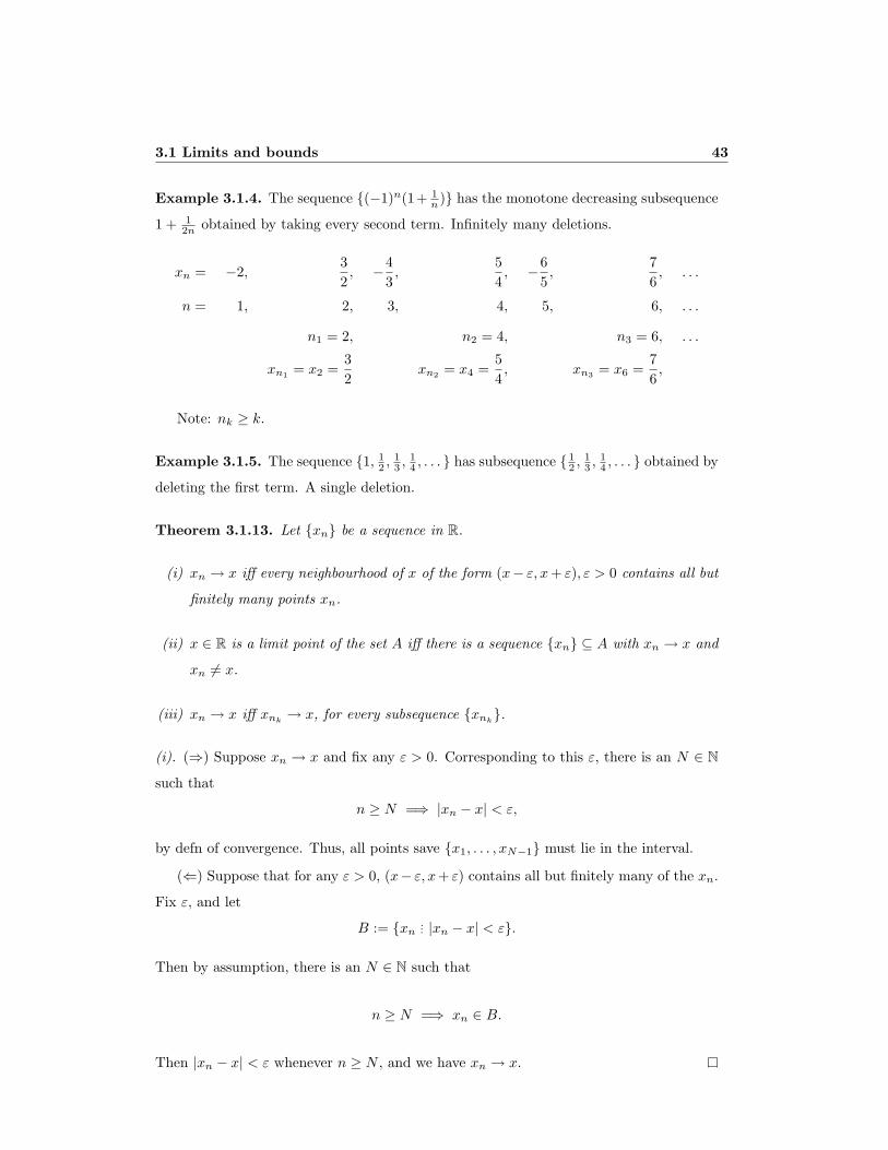
Example 3.1.4. The sequence {(−1)n(1+ 1n )} has the monotone decreasing subsequence

1 + 12n obtained by taking every second term. Infinitely many deletions.

xn = −2,32, −4

3,

54, −6

5,

76, . . .

n = 1, 2, 3, 4, 5, 6, . . .

n1 = 2, n2 = 4, n3 = 6, . . .

xn1 = x2 =32

xn2 = x4 =54, xn3 = x6 =

76,

Note: nk ≥ k.

Example 3.1.5. The sequence {1, 12 , 1

3 , 14 , . . . } has subsequence {1

2 , 13 , 1

4 , . . . } obtained by

deleting the first term. A single deletion.

Theorem 3.1.13. Let {xn} be a sequence in R.

(i) xn → x iff every neighbourhood of x of the form (x− ε, x + ε), ε > 0 contains all but

finitely many points xn.

(ii) x ∈ R is a limit point of the set A iff there is a sequence {xn} ⊆ A with xn → x and

xn 6= x.

(iii) xn → x iff xnk→ x, for every subsequence {xnk

}.

(i). (⇒) Suppose xn → x and fix any ε > 0. Corresponding to this ε, there is an N ∈ Nsuch that

n ≥ N =⇒ |xn − x| < ε,

by defn of convergence. Thus, all points save {x1, . . . , xN−1} must lie in the interval.

(⇐) Suppose that for any ε > 0, (x− ε, x+ ε) contains all but finitely many of the xn.

Fix ε, and let

B := {xn ... |xn − x| < ε}.

Then by assumption, there is an N ∈ N such that

n ≥ N =⇒ xn ∈ B.

Then |xn − x| < ε whenever n ≥ N , and we have xn → x.


(ii). (⇒) Fix ε > 0. For each n ∈ N, there is a point in A ∩ (x − 1n , x + 1

n ) which is not

x. Call it xn, so |xn − x| < 1n . Since 1

n decreases,

n ≥ N =⇒ |xn − x| < 1n≤ 1

N< ε.

Since we can choose N arbitrarily large, this shows xn → x.

(⇐) Immediate from the hypothesis and definition of limit point.

(iii). Homework.

Corollary 3.1.14 (to part (ii), above). x ∈ R is a limit point of the sequence {xn} ⊆ Riff there is a subsequence {xnk

} with xnk→ x.

Proof. Let A = {xn}. Note: the requirement xn 6= x is dropped because {an} allows for

repetition.

A sequence {xn} with limit point x is like a combination of a sequence which converges

to x with a bunch of “noise”. A sequence may have many limit points.

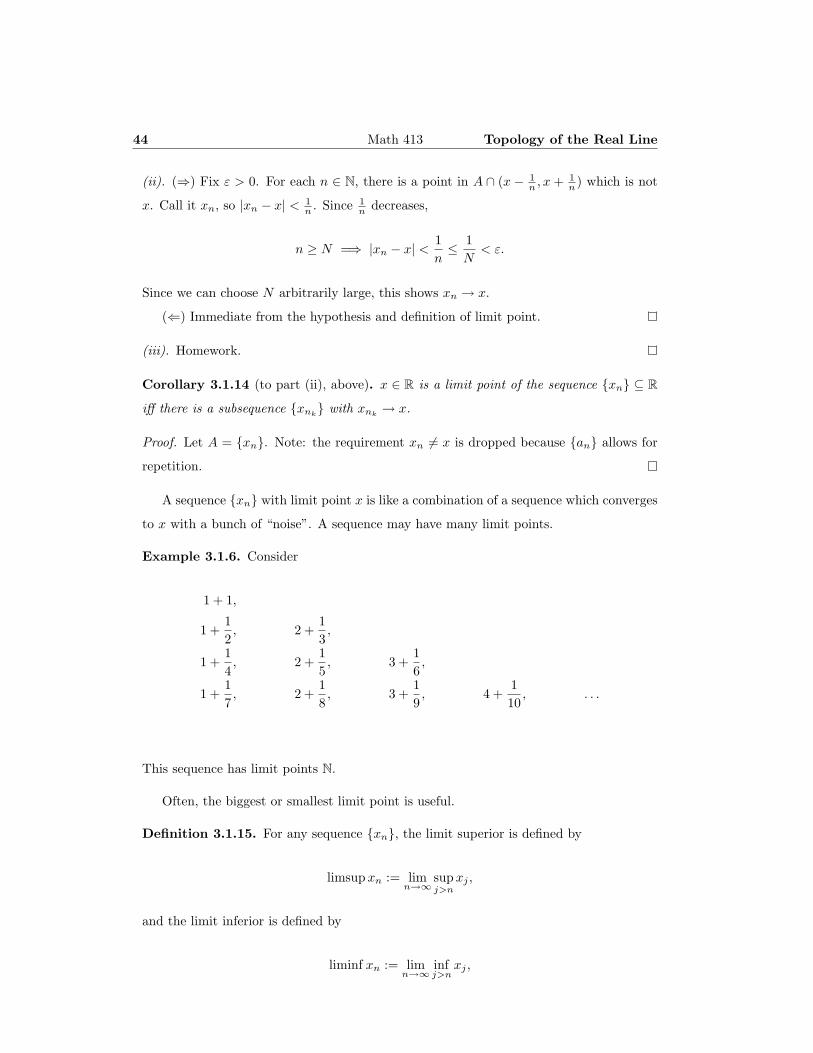
Example 3.1.6. Consider

1 + 1,

1 +12, 2 +

13,

1 +14, 2 +

15, 3 +

16,

1 +17, 2 +

18, 3 +

19, 4 +

110

, . . .

This sequence has limit points N.

Often, the biggest or smallest limit point is useful.

Definition 3.1.15. For any sequence {xn}, the limit superior is defined by

limsup xn := limn→∞

supj>n

xj ,

and the limit inferior is defined by

liminf xn := limn→∞

infj>n

xj ,


Example 3.1.7. Consider the sequence {xn} = {(−1)n(1+ 1n )}. We’ve seen that sup xn =

32 and inf xn = −2, but these don’t describe the limiting behavior of the sequence.

This sequence has limit points 1 and −1, so limsup xn = 1 and liminf xn = −1.

Theorem 3.1.16. (i) limsup xj is a limit point of {xj}.

(ii) limsup xj is the supremum of the set of limits points of {xj}.

Proof of (i). Let y = limsupxj , and start with the case y < ∞. Given n ∈ N, we can find

K such that

k ≥ K =⇒ |y − supj>k

xj | < 1n

.

Since y is finite, this shows supj>k xj is also finite, hence there is some x` satisfying

` > k, and |x` − supj>k

xj | < 1n

.

Together, |x`− supj>k xj | < 2n . By picking larger indices (say k1 > k) we can find another

point (say x`1 , `1 > `) satisfying the same criteria. Hence there are infinitely many, and

y is a limit point of the sequence.

If y = ∞, then {supj>k xj} is unbounded above. Thus {xj} is unbounded above, and

∞ is a limit point. If y = −∞, then for any −n, n ∈ N, there is K such that

k ≥ K =⇒ supj>k

xj < −n.

Since this shows there are infinitely many xj with xj ≤ −n, −∞ is a limit point.

Proof of (ii). Suffices to show that y = limsup xj is an upper bound, by Thm. 3.1.3 (a

contained upper bound is a max). Let x be a limit point, so that xjm → x for some

subsequence {xjm}. Since jk+1 > k, we have

yk = supj>k

xj = sup{xj ... j > k} ≥ xjk+1 =⇒ y ≥ x.

Theorem 3.1.17. {xn} converges iff liminf xn = limsup xn. (In this case, the common

value is limxn.)

Proof. (⇒) Fix ε > 0 and suppose xn → x converges. Then for |x| < ∞, we can find N

such that

n ≥ N =⇒ |xn − x| < ε.


This implies | supn>N xn − x| ≤ ε, so limsup xn = x. Similarly for liminf xn.

(⇐) Since

k ≥ N =⇒ infn>N

xn ≤ xk ≤ supn>N

xn,

we apply the Squeeze Thm to the hypotheses.

This theorem is extendable to the case xn → ±∞. For x = ∞, lim xn = limsup xn by

the prev thm. Also, the condition n ≥ N =⇒ xn > K implies that infk>n xk ≥ K →∞.

Similarly for x = −∞.

§3.1.3 Exercise: #3,4,9 Recommended: #2,5,12

1. If x is an upper bound of A and x ∈ A, then x = sup A.

2. Prove that the two definitions of limit point are equivalent.

3. Prove that the following is also an equivalent definition of limit point : given any

n,m ∈ N, there is a j ≥ m for which |x− xj | < 1n .

3.2 Open sets and closed sets 47

3.2 Open sets and closed sets

3.2.1 Open sets

QUESTION: Why are open sets handy? ANSWER: They have wiggle room.

Definition 3.2.1. limxn = L iff ∀ε > 0, ∃N, n ≥ N =⇒ |xn − L| < ε.

This is equivalent in R to a more general definition:

∀U (open interval containing L), ∃N such that n ≥ N =⇒ xn ∈ U.

REASON: L ∈ (a, b) =⇒ |L − a|, |L − b| > 0. Take ε to be the smaller of the two.

Then |xn − L| < ε =⇒ xn ∈ (a, b). Other direction is similar.

Definition 3.2.2. A set U is open iff every point of U lies in an open interval which is

contained in U , i.e., if

x ∈ U =⇒ ∃a, b such that x ∈ (a, b) ⊆ U.

This means open sets are automatically “big”: they contain uncountably many points;

contain EVERY point between the inf and sup of any subinterval. An open set automat-

ically has positive length.

Interpretation of defn: Roughly, no point of an open set lies on the boundary.

Definition 3.2.3. x is an interior point of A iff there is an open set U with x ∈ U ⊆ A.

So an alternative definition of open set is: A is open iff every point of A is an interior

point.

Example 3.2.1. (0, 1) is open because it does not contain its boundary points 0,1. If we

added 0, then and tiny interval (−ε, ε) about 0 will always contain negative numbers, so

(−ε, ε) * (0, 1). So [0, 1) is not open.

NOTE: two open intervals overlap by a positive amount, or else not at all. If overlap,

then the union is a single interval. If disjoint, then the union is two disjoint intervals.

Consider (a, b) and (c, d), where a < d. Two cases: b > c or b ≤ c.

Theorem 3.2.4. A set U ⊆ R is open iff it is a finite or countable union of disjoint open

intervals, i.e.,

U =N⋃

n=1

(an, bn), N may be ∞.


Proof. Define an open subinterval I ⊆ U to be maximal iff

I ⊆ (a, b) ⊆ U =⇒ I = (a, b).

Then let A be the collection of maximal intervals. It is clear that⋃

A∈AA ⊆ U . For the

reverse inclusion, consider the collection of subintervals of U that contain x. The union

of all of these is again a subinterval of U which contains x. Also, it is maximal. Thus

U ⊆ ⋃A∈AA.

Maximal intervals are disjoint (proof by contradiction).

Pick a rational number from each interval in A (by density of Q in R). (See HW)

Since maximal intervals are disjoint, these numbers are all distinct. So the cardinality of

A cannot exceed the cardinality of Q.

Theorem 3.2.5. Let A1, A2, . . . be open sets. Then

(i) Any union, like G =⋃

An, is open.

(ii) Any finite intersection, like F =⋂k

i=1 Ani , is open.

Proof of (i). Pick x ∈ G. Then ∃n, x ∈ An. Since An is open, can find an open interval

U with x ∈ U ⊆ An. Then x ∈ U ⊆ G.

Proof of (ii). This is trivial if the intersection is empty, so assume it isn’t. Then can pick

x ∈ F =⋂k

i=1 Ai, so ∀i = 1, . . . , k, x ∈ Ai. For each Ai, have x ∈ (bi, ci) ⊆ Ai. Define

b = max{bi} and c = min{ci}.KEY POINT: b < x < c, since these are finite sets! Then

x ∈ (b, c) ⊆ Ai,∀i = 1, . . . , k =⇒ x ∈ (b, c) ⊆⋂

Ai.

Example 3.2.2. Let An := (− 1n , 1 + 1

n ). Then

∞⋂n=1

An = [0, 1],

which is not open: there is no interval about 0 or 1 which is contained in the set.

Definition 3.2.6. A neighbourhood of x is an open set U with x ∈ U . Typically, we use

neighbourhoods of the form (x− ε, x + ε), but it need not be an interval.


Definition 3.2.7. The interior of A ⊆ R is

intA := {x ∈ A ... x ∈ (a, b) ⊆ A, for some a, b}.

x is an interior point of A iff x ∈ intA.

It is obvious that every set contains its interior points. For a set to be open, it means

that every point is an interior point.

Theorem 3.2.8. x = lim xn iff every neighbourhood of x contains all but finitely many

points of {xn}.

Proof. Exercise: this is basically the same as the first theorem in this section.

Definition 3.2.9. x is a limit point of A iff every neighbourhood U of x contains a point

of A, other than x itself. For U open,

A′ := {x ... ∀U open nbd, {x} ( U ∩A}.

Write A′ for the set of limit points of A.

If a sequence has only a finite number of repetitions, this coincides with the defn of

limit point of a sequence:

{5, 5, 5, 5, 5, . . . }

has 5 as a limit point of the sequence, but not the set. (This is because of the requirement

{x} ( U ∩A.) See HW §3.2.3 #2.

Example 3.2.3. Every point of [0, 1] is a limit point.

2 is not a limit point of [0, 1] ∪ {2}.√

2 is a limit point of Q.

Definition 3.2.10. A set C is closed iff C contains all its limit points, i.e.,

x ∈ C ′ =⇒ x ∈ C.

Theorem 3.2.11. A set is open iff its complement is closed.

Proof. (⇒) Suppose A is open. Let x be a limit point of Ac. Then every neighbourhood

U of x contains a point of Ac and so is not contained in A, i.e., x is not an interior point

of A. Since A is open x ∈ Ac, i.e., Ac contains all its limit points.


(⇐) Suppose Ac is closed. Pick some x ∈ A, so that x /∈ Ac and hence x is not a

limit point of Ac. Then there is a neighbourhood U of x which does not intersect Ac, i.e,

U ⊆ A.

Example 3.2.4. 0 is a limit point of (0, 1), but isn’t an element of (0, 1]. So (0, 1] is not

closed. Is it open?

(0, 1]c = (−∞, 0] ∪ (1,∞)

1 is a limit point of this set which is not contained in it, so (0, 1]c not closed =⇒ (0, 1]

not open.

Alt: 1 has no open nbd contained in (0, 1]; no wiggle room to the right.

NOTE: two disjoint closed sets are separated by some positive distance, i.e., min{|x−y| ..

. x ∈ A, y ∈ B} > 0 whenever A,B are closed and disjoint.

Theorem 3.2.12. If C1, C2, . . . are closed sets, then

(i) Any intersection, like⋂

Cn, is closed.

(ii) Any finite union, like⋃k

i=1 Cni , is closed.

Proof of (i).⋂

Cn =⋂

(Ccn)c = (

⋃Cc

n)c. Ccn open =⇒ ⋃

Ccn open =⇒ ⋂

Cn closed.

Definition 3.2.13. The closure of a set is the union of the set and all its limit points:

A := A ∪A′.

Theorem 3.2.14. The closure of a set A is the intersection of all closed sets containing

A:

A =⋂

A⊆C

C, C closed.

Proof. (⊆) If x ∈ A ∪ A′, then x ∈ A or x ∈ A′. If x ∈ A, then x ∈ C trivially, for any

C ⊇ A, and done. So assume x ∈ A′. Let C be any closed set containing A. Then for

every open neighbourhood U of x, there is y ∈ U ∩ A ⊆ U ∩ C, y 6= x. Thus, x is a limit

point of C, and hence contained in C. Since C was any arbitrary closed set containing A,

this is true for all closed sets containing A, and hence for the intersection of them.

(⊇) We show x /∈ A∪A′ =⇒ x /∈ ⋂A⊆C C. So assume x ∈ (A∪A′)c = Ac ∩ (A′)c, so

that x /∈ A and x /∈ A′. Then we can find an open neighbourhood U of x which is disjoint

from A, i.e., U ⊆ Ac. Then A ⊆ U c, and U c is a closed set by prev thm. We need to show

that x ∈(⋂

A⊆C C)c

=⋃

A⊆C Cc, so we’re done.


Corollary 3.2.15. The closure of A is the smallest closed set containing A.

Definition 3.2.16. B is a dense subset of A iff A ⊆ B.

Example 3.2.5 (The Cantor Set). Define a nested sequence of sets Ck+1 ⊆ Ck by

C0 = [0, 1]

C1 = [0, 13 ] ∪ [ 23 , 1]

C2 = [0, 19 ] ∪ [ 29 , 1

3 ] ∪ [ 23 , 79 ] ∪ [ 89 , 1]

...

The Cantor set is C :=⋂∞

n=0 Cn.

Alternative definition: define f1(x) = x3 and f2(x) = x

3 + 23 . Then C is the unique

nonempty closed and bounded set for which f1(C) ∪ f2(C) = C.

Theorem 3.2.17. 1. The Cantor set is closed.

2. Every point of the Cantor set is a limit point.

3. The Cantor set is totally disconnected, i.e., it contains no open interval.

4. The Cantor set contains uncountably many points.

5. The Cantor set has measure zero (length 0) as seen by 1−∑j=1

(13

)j.

6. For x ∈ [0, 1], define the ternary expansion of x by

x =d1

3+

d2

9+

d3

27+ · · ·+ dn

3n+ · · · =

∞∑

k=1

dk

3k,

where dk ∈ {0, 1, 2}. Then the Cantor set consists of exactly those x ∈ [0, 1] which

have dk ∈ {0, 2}, ∀k.

§3.2.3 Exercise: #1,4,7,8,13 Recommended: #2,5,14 #7,13 are short-

answer.

1. Suppose U is open, C is closed, and K is compact.

(a) Is U \ C open? Is C \ U closed?

(b) Is U \K open? Is C \K compact?


(c) If V is open, can U \ V be open?

(d) If J is compact, can K \ J be compact?

2. Prove the theorems about the Cantor set, using whichever of the definitions seems

best.

3.3 Compact sets 53

3.3 Compact sets

Definition 3.3.1. A set K ⊆ R is compact iff every sequence {xn} ⊆ K has a cluster

point x ∈ K.

This is an abstract version of “small” just like open was an abstract version of “big”.

We will characterize compactness in R:

Theorem 3.3.2. A set K ⊆ R is compact iff it is closed and bounded.

but first, need two theorems.

Definition 3.3.3. Let A1, A2, . . . be a sequence of sets in R. This sequence is nested iff

A1 ⊇ A2 ⊇ . . . . If this is a sequence of intervals An = [an, bn] = {x ... an ≤ x ≤ bn}, then

this means

an ≤ an+1 ≤ bn+1 ≤ bn, ∀n.

Note:⋂∞

n=1 An = {x ... x ∈ An, ∀n}.

Theorem 3.3.4 (Nested Intervals Thm). Suppose that An = [an, bn] is a nested sequence

of intervals with lim(an − bn) = 0. Then⋂∞

n=1 An = {L}. Also, an → L and bn → L.

Proof. There are 5 steps.

(i) an ≤ bm for any n,m. Suppose an > bm. Then

n > m =⇒ bn ≤ bm < an<↙

n < m =⇒ bm < an ≤ am<↙

(ii) {an} is increasing by nestedness, and bounded by (i), so converges by completeness.

Thus, let L = lim an.

(iii) ∀n, an ≤ L ≤ bn. Part (ii) shows an ≤ L

(EXERCISE: an ↗ L =⇒ an ≤ L)

an ≤ bm =⇒ L ≤ bm by Limit Location Thm.

(iv) L is the only number common to all intervals and bn → L.

Add the two convergent sequences {bn − an} and {an} to get

lim bn = lim((bn − an) + an) = lim(bn − an) + lim an = 0 + L = L.


Theorem 3.3.5 (Bolzano-Weierstrass). A bounded sequence in R has a convergent sub-

sequence.

Proof. Suppose {xn} is bounded, so that

a0 ≤ xn ≤ b0, ∀n.

By a previous theorem, suffices to find a cluster point of the sequence.

Apply the bisection method (aka divide-and-conquer): let c e the midpoint of [a0, b0].

Then at least one of [a, c] or [c, b0] contains infinitely many points xn; call it [a1, b1].

(Choose the first one, if both have infinitely many.) Continuing, we get a nested sequence

[a0, b0] ⊇ [a1, b1] ⊇ . . . ⊇ [am, bm] ⊇ . . .

Since

|bn − an| = |b0 − a0|2n

→ 0,

the Nested Intervals Thm gives

∃!L ∈⋂

[an, bn].

Claim: L is a cluster point of {xn}. Given ε > 0, choose N large enough that |bn−an| < ε.

Then [an, bn] ⊆ (L− ε, L + ε) and contains infinitely many of the xn.

Theorem 3.3.6. A set K ⊆ R is compact iff it is closed and bounded.

Proof. (⇒) Use contrapositive: K not (closed and bounded) implies K not compact. So

assume K is either not closed or not bounded; we show that K contains a sequence with

no limit point in K (just need one).

case (1) K is not closed. Then there is some limit point x of K, and x /∈ K. Since

x is a limit point, we can always find an ∈ (x − 1n , x + 1

n ) satisfying an ∈ K and

an 6= x. By construction, the only possible limit point of {an} is x, but x /∈ K.

case (2) K is not bounded. Then for each n ∈ N, there is an ∈ K with |an| > n.

Then an can have no limit point in R, and certainly not in K.

(⇐) Suppose K is closed and bounded and let {xn} be any sequence in K. Then the

Bolzano-Weierstrass Theorem gives a convergent subsequence {xnk} with xnk

→ x ∈ K.

Then x ∈ K is a limit point of K.

3.3 Compact sets 55

Corollary 3.3.7. Any infinite subset of a compact set has a cluster point.

Proof. This comes from the two previous theorems

Definition 3.3.8. An open cover of A ⊆ R is a collection of open sets {Ui} with A ⊆ ⋃Ui.

Example 3.3.1. (0, 1) ⊆ (0, 1) ⊆ (−1, 2).

(0, 1) ⊆ (0, 23 ) ∪ ( 1

3 , 1).

(0, 1) ⊆ ⋃n( 1

n , 1− 1n ).

R ⊆ ⋃n(−n, n).

U ⊆ ⋃x∈U (x− ε, x + ε).

Theorem 3.3.9. Let K ⊆ R be compact, and let B be a closed subset of K. Then B is

compact.

Proof. K is closed and bounded, by thm, so B ⊆ K must also be bounded. Since B is

closed by hypothesis, B is compact.

Theorem 3.3.10 (Heine-Borel Thm). A set is compact iff every open cover has a finite

subcover.

Proof. (⇒) Suppose A is an open cover of a compact set K. First, reduce A to a countable

subcover B. Let I be any open interval with rational endpoints. If there is an open set of

A which contains I, then add it to B. If not, then don’t. Now any point of K is contained

in an open interval with rational endpoints, and hence contained in one of the sets from

A that was added to B. So B ⊆ A is a subcover of K which is at most countable, so

B = B1, B2, . . . .

If B is finite, we are done, so suppose not. Then for each n ∈ N, we can choose a

point xn ∈ K which is not contained in⋃n

k=1 Bk. Then we have a subsequence xnk→

x ∈ K, by compactness. Since x ∈ K ⊆ ⋃Bk, we have x ∈ BN for some N . But

{xN , xN+1, xN+2, . . . } ⊆ BcN by construction. <↙

(⇐) Note that⋃∞

n=1(−n, n) is an open cover of R, hence also of K. Since we are

assuming the subcover property, we have K ⊆ (−n, n) for some n >> 1. So K is bounded.

To see K is closed, we show Kc is open.

Pick x ∈ Kc. We must produce an open set U such that x ∈ U ⊆ Kc, i.e., an open

neighbourhood U of x which is disjoint from K.


For each point y ∈ K, separate x from y by open sets: choose open neighbourhoods

of Uy of x and Vy of y which are disjoint (Ux ∩ Vy = ∅). Since U :=⋂

Uy is disjoint from

K, we would like to use this as a neighbourhood of x:

x ∈ U ⊆ Kc =⇒ x is an interior point of Kc.

Problem: an arbitrary intersection need not be open.

Meanwhile, {Vy} is an open cover of K. By the compactness of K, there must be

some finite open subcover of K which we can denote by {Vi}ni=1. Then by looking at the

neighbourhoods of x which correspond to these sets Vi, we have Ui∩Vi = ∅, ∀i = 1, . . . , n.

Since(⋂n

j=1 Uj

)⊆ Ui,∀i = 1, . . . , n, we have

(⋂Ui

)∩ Vi = ∅, ∀i =⇒

(⋂Ui

)∩

⋃Vi = ∅.

Thus

K ⊆⋃

Vi =⇒(⋂

Ui

)is disjoint from K.

Moreover, since (⋂n

i=1 Ui) is a finite intersection of open sets, it is also open. Therefore,

we can take U =⋂n

i=1 Ui as our open neighbourhood of x which is disjoint from K.

Theorem 3.3.11. A nested sequence A1 ⊇ A2, . . . of nonempty compact sets has a

nonempty intersection.

Proof. For each n, choose a xn ∈ An. Then {xn} ⊆ A1 by nesting, so it has a limit point

x ∈ A1 (since A1 is compact). But x is also a limit point of {xn, xn+1, . . . }, so x ∈ An.

Etc, x ∈ ⋂An.

Theorem 3.3.12. Let K be compact, and let B be a closed subset of K. Then B is

compact. (Same as earlier, but now don’t require K ⊆ R.)

Proof. Let {Uα}α∈A be an open cover of B. We need to find a finite subcover. Since B is

closed, we know that its complement Bc is open. Then

{Uα}α∈A ∪ {Bc}

is an open cover of the whole set K, and hence has a finite open subcover

{Ui}ni=1 ∪ {Bc}.

3.3 Compact sets 57

Since Bc doesn’t cover any part of B, we can throw it out and still have that

{Ui}ni=1

is an open cover of B. This is a finite subcover for B, i.e., B is compact.

Example 3.3.2. Define An = (0, 1n ). Then

⋂An = ∅.

3.3.1 Key properties of compactness

K ⊆ R is compact iff

1. Every sequence {xn} ⊆ K has a limit point x ∈ K.

2. K is closed and bounded.

3. Every open cover of K has a finite subcover.

Later, after we’ve seen continuity, we’ll also want

Theorem 3.3.13.

Let f : X → R be continuous, and let K ⊆ X be compact. Then there exist points

m,M ∈ K such that f(m) ≤ f(x) ≤ f(M), ∀x ∈ K.

Example 3.3.3. f(x) : (0, 1) → R by f(x) = x2 or f(x) = 1x .

Theorem 3.3.14. Let f : K → Y be continuous, where K is compact. Then f(K) is

compact in Y .

Theorem 3.3.15. On a compact set, any continuous function is automatically uniformly

continuous.

§3.3.3 Exercise: #4,8 Recommended: #3,6,10

#3 is short-answer; a rigorous proof is not required.

1. If F is closed and K is compact, then F ∩K is compact.


2. Suppose K = {Kα} is a collection of compact sets. if K has the property that

the intersection of every finite subcollection is nonempty, then prove that⋂

Kα is

nonempty. (Try contradiction or DeMorgan’s.)

3. Suppose that every point of the nonempty closed set A is a limit point of A. Show

that A is uncountable. (Try contradiction, and use the previous problem.)

Chapter 4

Continuous functions

4.1 Concepts of continuity

4.1.1 Definitions

Definition 4.1.1. 1 A function from a set D to a set R is a subset f ⊆ D×R for which

each element d ∈ D appears in only one element (d, ·) ∈ f . Write f : D → R. If (x, y) ∈ f ,

then we usually write f(x) = y.

D is the domain of the function; the subset of R of elements x for which the function is

defined.

R is the range; a subset of R which contains all the points f(x). Generally, assume R = R.

Definition 4.1.2. A function is a rule of assignment x 7→ f(x), where for each x in the

domain, f(x) is a unique and well-defined element of the range.

f(x) = y means “f maps x ∈ D to f(x) ∈ R”.

Definition 4.1.3. The image of f is the subset

Im f := {y ∈ R ... ∃x ∈ D, f(x) = y} ⊆ R.

The function f is surjective or onto iff Im f = R, that is,

∀y ∈ R, ∃x ∈ D, f(x) = y.

1May 2, 2007

60 Math 413 Continuous functions

Definition 4.1.4. For f : D → R, the preimage of B ⊆ R is the subset

f−1(B) := {x ... f(x) ∈ B} ⊆ D.

Example 4.1.1. The preimage of [0, 1] under f(x) = x2 is [−1, 1].

The preimage of [−1, 1] under f(x) = sin x is R.

The preimage of {1} under f(x) = sin x is {2kπ}k∈Z.

The preimage of [0, 1] under log x is [1, e].

Definition 4.1.5. A function f is injective or one-to-one iff no two distinct points in D

get mapped onto the same point in R, i.e.

f(x) = f(y) =⇒ x = y.

Example 4.1.2. f(x) = x2 is injective on (0,∞) but not on R.

f(x) = 1x is injective on R \ {0}.

A function is usually described by a formula or by its graph. If the graph is a connected

curve, we want to call the function continuous. To formalize:

x ≈ y =⇒ f(x) ≈ f(y).

Definition 4.1.6. f is continuous at x ∈ D iff

∀ε > 0,∃δ, |x− t| < δ =⇒ |f(x)− f(t)| < ε.

Write limt→x f(t) = f(x).

IDEA: |x− t| < δ means “t → x”, and |f(x)− f(t)| < ε means “f(t) → f(x)”, i.e.

t → x =⇒ f(t) → f(x).

Example 4.1.3. Define the Heaviside function

H(x) =

0, x < 0

1, x ≥ 0.

H is not continuous at 0: pick ε = 12 . If t < 0, then no matter how small |x− t|, we still

4.1 Concepts of continuity 61

have

|f(x)− f(t)| = |1− 0| = 1 >12

= ε,

so f(t) 9 f(x).

MORAL: the defn of continuity prevents a function from changing too rapidly; |f(x)|cannot “jump”.

Definition 4.1.7. f is a continuous function iff it is continuous at each x in its domain,

i.e.,

∀ε > 0, ∀x, ∃δ, |x− t| < δ =⇒ |f(x)− f(t)| < ε.

Strengthen this idea by disallowing a function from growing faster than a “globally

controlled” rate.

Definition 4.1.8. f is uniformly continuous on D iff

∀ε > 0, ∃δ,∀x, |x− t| < δ =⇒ |f(x)− f(t)| < ε.

This δ depends only on ε, not on x; thus, it works for ALL x simultaneously. NOTE:

uniformly continuous is a global property; it makes no sense to ask if f is uniformly

continuous at x0.

Example 4.1.4. f(x) = x2 is not uniformly continuous on R.

¬(∀ε > 0,∃δ,∀x, (|x− t| < δ =⇒ |f(x)− f(t)| < ε))

∃ε > 0,∀δ,∃x, ¬(|x− t| < δ =⇒ |f(x)− f(t)| < ε)

∃ε > 0,∀δ,∃x, (|x− t| < δ and |f(x)− f(t)| ≥ ε), (for some t).

Let δ > 0 be fixed. Then for points t of the form x + δ2 , we have |x − t| = |x − x + δ

2 | =δ/2 < δ. However,

|f(x)− f(t)| = |x2 − (x + δ)2| = |2xδ − δ2| = 2δ(x− δ) ≮ ε, x >> 1.

4.1.2 Limits of functions and limits of sequences

Continuous functions are useful because they preserve limits:

limt→x

f(t) = f(limt→x

t) = f(x),


i.e., f is a continuous function iff it takes convergent sequence to convergent sequences.

Theorem 4.1.9. limt→x f(t) = L iff limn→∞ f(xn) = L for every {xn} with xn → x

Proof. (⇒) Choose a sequence xn → x, and fix ε > 0. Since f is continuous, ∃δ > 0 for

which

|x− t| < δ =⇒ |f(t)− L| < ε.

Also, there is N such that

n ≥ N =⇒ |xn − x| < δ.

Thus, n ≥ N =⇒ |f(xn)− L| < ε.

(⇐) Contrapositive: suppose it is false that limt→x f(t) = L. Then:

∃ε > 0,∀δ > 0,∃t, |x− t| < δ and |f(t)− L| ≥ ε

∃ε > 0, ∀n ∈ N,∃tn, |x− tn| < 1n and |f(tn)− L| ≥ ε

This produces tn → x for which it is false that limn→∞ f(xn) = L.

Corollary 4.1.10. If f has a limit at x, this limit is unique.

Proof. Combine prev thm with uniqueness thm for sequences.

4.1.3 Inverse images of open sets

Theorem 4.1.11. Suppose the domain of f is open. f is continuous iff the preimage of

every open set is open.

Proof. (⇒) Let f be continuous and let V ⊆ R be open. Must show: every point of f−1(V )

is an interior point. Pick p ∈ D for which f(p) ∈ V . Since V is open, (f(p)−ε, f(p)+ε) ⊆ V

for some ε > 0. Since f is continuous, there is a δ > 0 such that

|x− p| < δ =⇒ |f(x)− f(p)| < ε.

Thus, x ∈ f−1(V ) as soon as |x− p| < δ, i.e. x ∈ (p− δ, p + δ) ⊆ f−1(V ).

(⇐) Suppose that V open in R implies that f−1(V ) is an open subset of D. Fix any

p ∈ D and ε > 0. Choose a specific V = (f(p) − ε, f(p) + ε). Then f−1(V ) open means

that p ∈ f−1(V ) is an interior point of f−1(V ). In particular, we can find δ > 0 such that

4.1 Concepts of continuity 63

x ∈ f−1(V ) as soon as x ∈ (p− δ, p + δ). But

x ∈ f−1(V ) =⇒ f(x) ∈ V =⇒ |f(x)− f(p)| < ε.

Corollary 4.1.12. f is continuous iff the preimage of every closed set is closed.

Proof. HW.

Connectedness

Definition 4.1.13. A set X is connected iff it CANNOT be written

X = A ∪B, A ∩B = ∅, A, B 6= ∅,

for two open sets A, B.

Theorem 4.1.14. The continuous image of a connected set is connected.

Proof. Let f : X → R be continuous, and let X be connected. Must show f(X) is

connected. Suppose, by way of contradiction, that f(X) = A∪B is a separation of f(X).

Then f−1(A) and f−1(B) are disjoint nonempty open sets whose union is X. <↙

A ∩B = ∅ =⇒ f−1(A ∩B) = ∅, because

x ∈ f−1(A ∩B) =⇒ x ∈ f−1(A) and x ∈ f−1(B) =⇒ f(x) ∈ A ∩B.

4.1.4 Related definitions

Definition 4.1.15. f is a Lipschitz function (or strongly continuous function) iff

|f(x)− f(y)| ≤ M |x− y|

for some constant M . (The Lipschitz constant.)

Then

|x− y| < ε

M=⇒ |f(x)− f(y)| < ε.


Definition 4.1.16. f is a Holder function (or satisfies a Holder condition of order α) iff

|f(x)− f(y)| ≤ M |x− y|α, 0 < α ≤ 1,

for some constant M . (The Lipschitz constant.)

NOTE: if α = 0, this would just say that f is bounded (with max variation M).

Then

|x− y| <( ε

M

)1/α

=⇒ |f(x)− f(y)| < ε.

NOTE: for α ≈ 0,(

εM

)1/α → 0 fast (ε < M).

Definition 4.1.17. f has a limit from the right at x (or is right-continuous at x) iff

∀ε > 0,∃δ, 0 < t− x < δ =⇒ |f(t)− L| < ε.

Write f(x+) := limt→x+ f(t) = L.

Similarly for f(x−) := limt→x− f(t):

∀ε > 0,∃δ, 0 < x− t < δ =⇒ |f(t)− L| < ε.

4.2 Properties of continuity 65

4.2 Properties of continuity

Theorem 4.2.1. If f, g are continuous, then so are f + g, f · g, and (if g 6= 0) f/g.

Proof. Continuous functions preserve sequences, and limits are linear & multiplicative for

sequences.

NOTE: Define (f + g)(x) := f(x) + g(x), etc.

USE this with the thm that lim commutes with continuous functions:

Example 4.2.1. NOTE: all limits are finite, and the denom 6= 0!

limt→1

3t2 −√t

t2 + 1=

limt→1(3t2 −√t)limt→1(t2 + 1)

=3 limt→1 t2 − limt→1

√t

limt→1 t2 + limt→1 1=

3−√limt→1 t

1 + 1=

22

= 1

Theorem 4.2.2. Let x = g(t), c = g(b). If g(t) is continuous at b and f(x) is continuous

at c, then f ◦g(t) = f(g(t)) is continuous at b.

Proof. Given ε > 0, ∃δ > 0 such that

f(x) ≈ε f(c) for x ≈δ c continuity of f

g(t) ≈δ g(b) for t ≈α b continuity of g.

Then t ≈α b =⇒ x = g(t) ≈δ g(b) = c =⇒ f(x) ≈ε f(c).

Theorem 4.2.3 (Pasting Lemma). Suppose f : A → R and g : B → R where A,B are

closed. If f(x) = g(x) for every x ∈ A ∩B, then h : A ∪B → R is continuous:

h(x) :=

f(x), x ∈ A

g(x), x ∈ B.

Proof. Suppose C ⊆ R is a closed set. By elementary set theory,

h−1(C) = f−1(C) ∪ g−1(C).

f continuous =⇒ f−1(C) closed, and g continuous =⇒ g−1(C) closed, so the finite

union h−1(C) is closed.

Theorem 4.2.4. If f, g continuous then so are max{f, g} and min{f, g}.


Proof. Apply the Pasting Lemma to

max{f, g}(x) :=

f(x), f(x) ≥ g(x)

g(x), g(x) ≥ f(x).

The intersection is the set where f = g by defn, so only remains to check the two sets are

closed.

{x ... f(x) ≥ g(x)} = {x ..

. f(x)− g(x) ≥ 0} = {x ... (f − g)(x) ≥ 0} = (f − g)−1 ([0,∞))

Theorem 4.2.5 (Intermediate Value Theorem). If f is continuous on [a, b], then f as-

sumes all values between f(a) and f(b).

Proof 1. If f(a) = f(b), it is trivial, so wlog let f(a) < f(b). Suppose c ∈ (f(a), f(b)).

Let

A := {x ... f(x) < c}

B := {x ... f(x) > c}.

Assume, by way of contradiction, that c /∈ f(a, b). Then A ∪ B = [a, b] and clearly

A ∩B = ∅. Since a ∈ A and b ∈ B, neither is empty. <↙[a, b] is connected.

Proof 2. Again, suppose c ∈ (f(a), f(b)) and ∀x, f(x) 6= c. Then A = (−∞, c), B = (c,∞)

is a disconnection of f([a, b]). <↙

Corollary 4.2.6. Let f be continuous on [a, b]. If f changes sign on the interval (say

f(a) < 0 < f(b)), then ∃c ∈ [a, b] for which f(c) = 0.

Example 4.2.2. A polynomial of odd degree has a real zero.

Proof. Consider x2k+1 = x(x2)k. Then

x < 0 =⇒ x(x2)k < 0, x > 0 =⇒ x(x2)k > 0.

Apply this to the polynomial a0 + a1x + . . . anxn, assuming an 6= 0 (so it has degree

n = 2k + 1). The lesser terms will not matter for |x| >> 1:

∣∣an−1xn−1 + · · ·+ a0

∣∣ ≤ |an−1|∣∣xn−1

∣∣ + · · ·+ |a0|


≤ |anxn|(∣∣∣∣

an−1

anx

∣∣∣∣ +∣∣∣∣an−2

anx2

∣∣∣∣ + · · ·+∣∣∣∣

a0

anxn

∣∣∣∣)

≤ |anxn|,

since the expression in parentheses is < 1 for x >> 1.

NEXT: The continuous image of a compact set is compact.

Theorem 4.2.7. Let f be continuous, where K is compact. Then f(K) is compact.

Proof. Let {Uα}α∈A be a covering of f(K) by open sets Uα. NTS: ∃ a finite subcover.

Since f is continuous, every set f−1(Uα) will be open in K.

Since the Uα cover f(K), we have an open cover {f−1(Uα)} of K.

K is compact by hypothesis, so there must be some finite subcover {f−1(Ui)}ni=1 of K.

K ⊆n⋃

i=1

f−1(Ui) =⇒ f(K) ⊆ f

(n⋃

i=1

f−1(Ui)

)by S&M 4(a)

=n⋃

i=1

f(f−1(Ui)

)by S&M 4(b)

⊆n⋃

i=1

Ui by S&M 1(b),

and we have f(K) contained in the finite subcover {Ui}ni=1. I.e., f(K) is compact.

Corollary 4.2.8. A continuous function on a compact set is bounded and attains its sup

and inf.

Proof. If K is compact, then so is f(K), by prev. So f(K) is closed and bounded.

Theorem 4.2.9. On a compact set, continuity and uniform continuity are equivalent.

Proof. It is clear that uniform continuity implies continuity. For the converse, fix ε > 0.

Since f is continuous, for each x in the domain, can find δx such that

|x− y| < δx =⇒ |f(x)− f(y)| < ε

2.

For each x, define a neighbourhood Ux to be a δx

2 -ball about x:

Ux := (x− δx

2 , x + δx

2 ).


Then {Ux} is an open cover, so there are finitely many points {x1, . . . , xn} such that {Uxi}

is a finite subcover. We have the corresponding numbers δi := δxi . Define

δ := mini=1,...,n

{ δi

2 }.

NOTE: finiteness here is why compactness is necessary — then δ > 0.

Now show this δ satisfies the defn of uniformly continuous: pick any p, q in the domain

with |p− q| < δ. Since {Uxi} is a cover,

∃i, p ∈ Uxi =⇒ |p− xi| < δi

2(∗)

Then

|q − xi| ≤ |q − p|+ |p− xi|

< δ +δi

2by (*)

≤ δi. (∗∗)

So by the initial defn of δi, (*) and (**) give

|f(p)− f(q)| ≤ |f(p)− f(xi)|+ |f(xi)− f(q)| < ε.

A monotone function on an interval has one-sided limits at all points of the domain,

finite except possibly at the endpoints.

Theorem 4.2.10. If f is monotonic increasing on (a, b), then for every x ∈ (a, b),

supa<t<x

f(t) = f(x−) ≤ f(x) ≤ f(x+) = infa<t<x

f(t).

Further, for a < x < y < b, f(x+) ≤ f(y−).

Proof. Let A := sup{f(t) ... a < t < x}. Since f(x) is an upper bound for the set, we know

A exists. To prove A = f(x−), fix ε > 0. Since A is a l-u-b, can find δ > 0 such that

a < x− δ < x and A− ε < f(x− δ) ≤ A.


Since f is monotonic,

f(x− δ) ≤ f(t) ≤ A for x− δ < t < x.

Combine prev two eqns to get |f(t)−A| < ε. Thus, A = f(x−).

Next, for a < x < y < b, monotonicity gives

supa<t<y

f(t) = supy−δ<t<y

f(t) = f(y−)

from which

f(x+) = infa<t<y

f(t) ≤ supa<t<y

f(t) = f(y−).

Corollary 4.2.11. A monotone function on an interval has at most a countable number

of discontinuities, all of which are jump discontinuities.

Proof. Wlog, let f be increasing, and let D be the set of discontinuities of f . For each

x ∈ D, associate a rational number r(x) such that f(x−) < r(x) < f(x+). Since

x < y =⇒ f(x+) ≤ f(y−),

the strict inequalities above give

x 6= y =⇒ r(x) 6= r(y).

r is injective, and thus gives a bijection between the jumps and a subset of Q.

§4 Exercise: #2,5,11 Recommended: #3,9

1. Show f is continuous iff the preimage of every closed set is closed.

2. Show that a continuous function is determined by its values on a dense subset of the

domain: let f, g : X → R be continuous, and let D be dense in X. Prove that f(D)

is dense in f(X) and that

(f(x) = g(x), ∀x ∈ D) =⇒ (f(x) = g(x), ∀x ∈ X).


3. Let I := [0, 1]. If f : I → I is continuous, show that f has a fixed point, i.e.,

∃x ∈ I, f(x) = x.

4. Consider the function which is 0 on every irrational, and takes the value 1n if x is a

rational written as mn in lowest terms:

f(x) =

0, x ∈ R \Q1n , x = m

n ∈ Q, n > 0.

Show that f is continuous at every irrational, and has a simple discontinuity at every

rational.

Chapter 5

Differentiation

5.1 Concepts of the derivative

1

5.1.1 Definitions

Definition 5.1.1. f is differentiable at x0 iff

∀ε > 0, ∃δ > 0|x− x0| < δ =⇒∣∣∣∣f(x)− f(x0)

x− x0− L

∣∣∣∣ < ε,

in which case f ′(x0) = L.

Since x 6= x0, multiply the inequality to obtain

Definition 5.1.2. f is differentiable at x0 iff

∀m > 0,∃n > 0|x− x0| < 1n

=⇒ |f(x)− (f(x0) + f ′(x0)(x− x0))| < |x− x0|m

.

So f ≈ g for g(x) = f(x0) + f ′(x0)(x− x0).

Definition 5.1.3. If f(x)g(x)

x→x0−−−−−→∞, then f “blows up” faster than g. If f(x)g(x)

x→x0−−−−−→ 0,

then g “blows up” faster than f ; write f(x) = o(g(x)).

Write f(x) = O(g(x)) iff f(x)g(x) ≤ b < ∞ as x → x0.

1May 2, 2007

72 Math 413 Differentiation

Then “f is differentiable” means f(x) − g(x) = o(|x − x0|), where g is the affine

approximation to f : g(x) = f(x0) + f ′(x0)(x− x0).

5.1.2 Continuity and differentiability

Theorem 5.1.4. f is differentiable at x0 implies f is continuous at x0.

Proof. f(t)− f(x) =f(t)− f(x)

t− x· (t− x) → f ′(x) · 0 = 0.

In fact, f must be Lipschitz.

Definition 5.1.5. f is differentiable on an open set U iff it is differentiable at every point

of U . f is C1 on U iff f ′ is continuous on U and Ck iff f (k) is continuous on U .

NOTE: f ∈ C0 means that f is continuous.

Example 5.1.1. A function which is C2 but not C3 on R:

f(x) =

x2

2 + x + 1, x ≤ 0

ex, x ≥ 0.

5.2 Properties of the derivative 73

5.2 Properties of the derivative

5.2.1 Local properties

Definition 5.2.1. f is monotone increasing at x iff f(s) ≤ f(x) ≤ f(t) for a < s < x <

t < b. f is strictly increasing at x iff f(s) < f(x) < f(t) for a < s < x < t < b.

Proposition 5.2.2. f is (monotone or strictly) increasing on (a, b) iff f is order-preserving

on (a, b).

Proof. Immediate.

Definition 5.2.3. f has a local maximum at x iff f(t) ≤ f(x), for all t ∈ (x− ε, x + ε).

f has a strict local maximum at x iff f(t) > f(x), for all t 6= x in (x− ε, x + ε).

Theorem 5.2.4. If x is a local max or min of f , then f ′(x) = 0.

Proof. Choose δ such that a < x− δ < x < x + δ < b. Then for x− δ < t < x, we have

f(t)− f(x)t− x

≥ 0.

Letting t → x, get f ′(x) ≥ 0. Similarly for the other inequality.

Example 5.2.1. f(x) = x3 is strictly increasing, but has derivative 0 at 0.

Also, f doesn’t have a max or min at 0.

Theorem 5.2.5 (Rolle’s). If f is continuous on [a, b] and differentiable on the interior

and f(a) = f(b), then ∃x ∈ (a, b) such that f ′(x) = 0.

Proof. If f is constant on the interval, we are done, so wlog let h(t) > h(a) somewhere.

Then f attains its max at some point x ∈ (a, b) (since f([a, b]) is compact), and the prev

thm gives f ′(x) = 0.

5.2.2 IVT and MVT

Theorem 5.2.6 (Continuity of derivatives). f is differentiable on (a, b). Then f ′ assumes

every value between f ′(s) and f ′(t), for a < s < t < b.

Proof. Let λ ∈ (f ′(s), f ′(t)), and define g(t) = f(t)− λt so that

g′(a) = f(a)− λ < 0 =⇒ g(t1) < g(a) for some a < t1 < b, and


g′(b) = f(b)− λ > 0 =⇒ g(t2) < g(b) for some a < t2 < b.

Then g attains its min on [a, b] at some point x such that a < x < b. It follows that

g′(x) = 0, hence f ′(x) = λ.

Corollary 5.2.7. If f is differentiable on [a, b], then f ′ cannot have any simple or jump

discontinuities on [a, b].

Theorem 5.2.8 (Cauchy mean value thm). f, g are continuous on [a, b] and differentiable

on the interior. Then ∃x ∈ (a, b) for which

[f(b)− f(a)]g′(x) = [g(b)− g(a)]f ′(x).

Proof. Define

h(t) := [f(b)− f(a)]g(t)− [g(b)− g(a)]f(t) a ≤ t ≤ b

so that h is continuous on [a, b] and differentiable on the interior and

h(a) = f(b)g(a)− f(a)g(b) = h(b).

By Rolle’s Thm, get h′(x) = 0 for some x.

Interp: x = f(s), y = g(t) (SKETCH).

Corollary 5.2.9 (“The” Mean Value Thm). If f continuous on [a, b] and differentiable

on the interior, then ∃x ∈ (a, b) for which

f(b)− f(a) = (b− a)f ′(x).

Theorem 5.2.10. f is differentiable on (a, b).

1. If f ′(x) ≥ 0,∀x ∈ (a, b), then f is increasing.

2. If f ′(x) ≤ 0,∀x ∈ (a, b), then f is decreasing.

3. If f ′(x) = 0,∀x ∈ (a, b), then f is constant.

Proof. These can all be read off from the equation

f(t)− f(s) = (t− s)f ′(x),

5.2 Properties of the derivative 75

which is always valid for some x ∈ (s, t).


5.3 Calculus of derivatives

5.3.1 Arithmetic rules

Theorem 5.3.1 (Linearity).

f, g differentiable at x =⇒ (af + bg)′(x) = af ′(x) + bg′(x),∀a, b ∈ R.

Proof. HW (follows immediately from limit defn)

Theorem 5.3.2 (Product rule).

f, g differentiable at x =⇒ (fg)′(x) = f ′(x)g(x) + f(x)g′(x).

Proof. Let h = fg so that

h(t)− h(x) = f(t)g(t)− f(t)g(x) + f(t)g(x)− f(x)g(x)

h(t)− h(x)t− x

=f(t)[g(t)− g(x)]

t− x+

g(x)[f(t)− f(x)]t− x

.

Theorem 5.3.3 (Quotient rule).

f, g differentiable at x, g(x) 6= 0 =⇒(

fg

)′(x) = f ′(x)g(x)−f(x)g′(x)

g2(x) .

Proof. HW: Let h = f/g so that

h(t)− h(x)t− x

=1

g(t)g(x)

[g(x)

f(t)− f(x)t− x

− f(x)g(t)− g(x)

t− x

].

Theorem 5.3.4 (Chain Rule). If f is differentiable at x and g is differentiable at f(x),

then g◦f is differentiable at x with (g◦f)′(x) = g′(f(x))f ′(x).

Proof. Let y = f(x) and s = f(t) and define h(t) = g(f(t)). By the defn of derivative,

f(t)− f(x) = (t− x)[f ′(x) + o(1)] as t → x

g(s)− g(y) = (s− y)[g′(y) + o(1)] as s → y.

So : h(t)− h(x) = g(f(t))− g(f(x))

= (s− y)[g′(y) + o(1)]

= [f(t)− f(x)] [g′(f(x)) + o(1)]

= [(t− x)[f ′(x) + o(1)]] [g′(f(x)) + o(1)]

h(t)− h(x)t− x

= [f ′(x) + o(1)][g′(f(x)) + o(1)].

5.3 Calculus of derivatives 77

Note: s → y as t → x, by continuity of f .

Theorem 5.3.5 ((Baby) Inverse Fn Thm). f : (a, b) → (c, d) is C1 and f ′(x) > 0 on

(a, b). Then f is invertible and is C1 with (f−1)′(y) = 1/f ′(x), if y = f(x).

Proof. Use the chain rule to differentiate both sides of the identity f−1(f(x)) = x.


5.4 Higher derivatives and Taylor’s Thm

5.4.1 Interpretations of f ′′

Definition 5.4.1. If f ′ is defined in a neighbourhood of x and differentiable at x, then f

is twice differentiable at x, with f ′′(x) = (f ′)′(x). If f ′′ is continuous, then f ∈ C2.

Theorem 5.4.2. Suppose f ′′ exists in some neighbourhood of x.

(i) f ′(x) = 0, f ′′(x) > 0 =⇒ x is a strict local min.

(ii) If x is a local max, then f ′′(x) ≤ 0.

(iii) f ′′(x) > 0 =⇒ the graph of f(x) lies below any secant line.

Proof. (i) f ′′(x) > 0 means f ′ is increasing on some open interval (a, b) around x, with

f ′(a) < 0 and f ′(b) > 0 (since f ′(x) = 0). Then f is decreasing on (a, x) and

increasing on (x, b).

(ii) This is implied by the contrapositive of (1).

(iii) Let g be an affine function whose graph intersects f ’s at x = s and x = t. We need

to show f(x) < g(x), i.e. that h := f − g is negative on (s, t) (note h(s) = h(t) = 0).

If f ′′(x) > 0 for a < x < b, then h is also, since g′′ = 0. Suppose h were not negative

on (s, t); then it would have a local max on this interval at some point c. By Part

(1), this would imply h′′(c) ≤ 0. <↙

Part (i) holds, in particular, for g(t) = f(x) + f ′(x)(x− t).

5.4.2 Taylor’s Thm

Definition 5.4.3. If f ∈ Cn, the Taylor expansion of f at a is

Tn(a, x) = f(a) + f ′(a)(x− a) +12f ′′(a)(x− a)2 + · · ·+ 1

n!f (n)(a)(x− a)n,

where f (n) = (f (n−1))′ is defined by induction.

Theorem 5.4.4. If f (n) exists at a, then Tn(a, x) is the unique polynomial of degree n in

powers of (x− a) having nth-order agreement with f(x) at a.

5.4 Higher derivatives and Taylor’s Thm 79

Proof. Suppose p is a polynomial in (x− a):

p(x) = c0 + c1(x− a) + · · ·+ cn(x− a)n.

After k differentiations, the terms c0, . . . , ck−1 vanish:

p(k)(x) = k!ck + (terms with (x− a) as a factor).

So p(k)(a) = k!ck. If f(x) and p(x) have nth-order agreement,

f (k)(a) = k!ck =⇒ ck =f (k)(a)

k!, ∀k = 1, . . . , n.

Theorem 5.4.5 (Taylor’s Thm). Suppose f ∈ Cn+1(I) for some open interval I contain-

ing a and x. Then for some c between a and x,

f(x) = f(a) + f ′(a)(x− a) +12f ′′(a)(x− a)2 + · · ·+ 1

n!f (n)(a)(x− a)n + Rn(x),

Rn(x) =f (n+1)(c)(n + 1)!

(x− a)n+1.

NOTE: c depends on x, so RHS of f is not a polynomial; f (n+1)(c) is not a constant.

Proof. We show the theorem holds at x = b. Let P be defined by

P (x) = Tn(a, x) + C(x− a)n+1,

where C is chosen so that f(b) = P (b), i.e., C = f(b)−Tn(a,b)(b−a)n+1 . Let

g(x) = f(x)− P (x)

so that g(a) = g(b) = 0. Must show f (n+1)(c) = (n + 1)!C for some c ∈ (a, b). Since

g(n+1)(x) = f (n+1)(x)− (n + 1)!C, suffices to find a zero of g(n+1) on (a, b).

Since T(k)n (a) = f (k) for k = 0, . . . , n, we have

g(a) = g′(a) = · · · = g(n+1)(x) = 0.


Applying the MVT n times to the derivatives of g,

g(x) = g′(x1)(x− a)

g′(x1) = g′′(x2)(x1 − a)

...

g(n)(xn) = g′(xn+1)(xn − a),

each time using g(k)(xk) = 0 and the fact that f ∈ Cn =⇒ g ∈ Cn. Then g(n+1)(xn) = 0

for xn ∈ (a, b).

Corollary 5.4.6. f = Tn + o(|x− a|n) as x → a.

Theorem 5.4.7 (L’Hopital’s Rule). Suppose f, g ∈ C1(a, b) satisfy limx→c f(x) = limx→c g(x) =

0 for c ∈ (a, b). If g′(c) 6= 0, then

limx→c

f(x)g(x)

= limx→c

f ′(x)g′(x)

.

Proof. We only need to take the limit of

f(x)g(x)

=f(c) + f ′(c)(x− c) + o(|x− c|)g(c) + g′(c)(x− c) + o(|x− c|) Taylor’s Thm

=f ′(c)(x− c) + o(|x− c|)g′(c)(x− c) + o(|x− c|) continuity

=f ′(c) + o(1)g′(c) + o(1)

cancellation.

Theorem 5.4.8 (L’Hopital’s Other Rule). Suppose f, g ∈ C1(a, b) satisfy limx→c f(x) =

limx→c g(x) = ∞, then the same result holds.

§5 Exercise: # Recommended: #

1. Prove the linearity of differentiation.

2. Prove the quotient rule.

Chapter 6

Integration

6.1 Integrals of continuous functions

1

6.1.1 Existence of the integral

Let f(x) be a function defined on [a, b]. We want to define its integral∫ b

af(x) dx.

Definition 6.1.1. A partition P of the interval [a, b] is a finite set of points {a =

x0, x1, x2, . . . , xn = b}, xi < xi+1.

Definition 6.1.2. On each subinterval [xi, xi+1], of the partition P , define

Mi = sup f(x) xi−1 ≤ x ≤ xi

mi = inf f(x) xi−1 ≤ x ≤ xi

U(f, P ) =n∑

i=1

Mi(xi − xi−1)

L(f, P ) =n∑

i=1

mi(xi − xi−1)

U(f, P ) is the upper sum of f on the partition P , and L(f, P ) is the lower sum of f on

the partition P .

1May 2, 2007

82 Math 413 Integration

Definition 6.1.3. If supP L(f, P ) = infP U(f, P ), then the integral of f on [a, b] is defined

to be the common value, denoted∫ b

af(x) dx. We say f is (Riemann-) integrable on [a, b]

and write f ∈ R[a, b].

Definition 6.1.4. The partition P ′ is a refinement of P iff P ⊆ P ′.

Note that adding points to the partition has two effects:

1. the lengths of the subintervals decreases, and

2. L(f, P ) increases and U(f, P ) decreases.

Theorem 6.1.5. For P ⊆ P ′, L(f, P ′) ≥ L(f, P ) and U(f, P ) ≤ U(f, P ).

Proof. Do the case where P ′ = P ∪ {y} first; then the sums only change on the one

subinterval. General case by repetition.

Suppose we have a nested sequence of partitions P1 ⊆ P2 ⊆ . . . . Then {L(f, Pi)} and

{U(f, Pi)} are monotonic sequences, each bounded by any element of the other. So both

converge. f is integrable when they converge to the same value.

Definition 6.1.6. The oscillation of f is Osc(f, P ) = U(f, P )− L(f, P ).

Next:∫ b

af(x) dx exists iff Osc(f, Pn) → 0, for some nested sequence {Pn}.

Theorem 6.1.7 (Oscillation). f ∈ R[a, b] iff ∀ε > 0, ∃P such that Osc(f, P ) < ε.

Proof. (⇒) Let f ∈ R and fix ε > 0. Then there are partitions P1, P2 such that

U(f, P1)−∫

f < ε

∫f − L(f, P1) < ε.

Let P = P1 ∪ P2 be the common refinement. Then

U(f, P ) ≤ U(f, P2) <

∫f + ε < L(f, P1) + 2ε ≤ L(f, P ) + 2ε,

so that U(f, P )− L(f, P ) < 2ε.

(⇐) Apply the inequality U(f, P )− L(f, P ) < ε to

L(f, P ) ≤ supP

L(f, P ) ≤ infP

U(f, P ) ≤ U(f, P )

to get 0 < infP U(f, P )− supP L(f, P ) < ε. Since this is true for any ε > 0, done.

6.1 Integrals of continuous functions 83

Definition 6.1.8. A norm on a vector space is a function from X to R that satisfies

(i) ‖x‖ ≥ 0, ‖x‖ = 0 ⇐⇒ x = 0.

(ii) ‖ax‖ = |a| · ‖x‖,∀a ∈ R.

(iii) ‖x− z‖ ≤ ‖x− y‖+ ‖y − z‖, ∀x, y, z ∈ X.

Example 6.1.1. On R, absolute value is a norm.

For x = (a, b) ∈ R2, ‖x‖ =√

a2 + b2.

For f ∈ R(D), ‖f‖1 :=∫

D|f(x)| dx.

Definition 6.1.9. A step function is one which is locally constant except for finitely many

points. Thus, a step function is usually defined in terms of a partition; it is constant on

each subinterval and can have a jump discontinuity at each point of the partition.

Example 6.1.2. Define the step functions

fP (x) = infxi−1≤x≤xi

f(x) and fP (x) = supxi−1≤x≤xi

f(x).

Then the previous theorem states that f is integrable iff there is a sequence of partitions

{Pn} with ∫|fPn(x)− fPn(x)| dx

n→∞−−−−−→ 0.

Since we can always take a common refinement of two partitions, this amounts to

saying that f is integrable iff it can be approximated by step functions, i.e.,

∀ε > 0,∃g ∈ Step, n ≥ N =⇒ ‖f − g‖1 < ε.

Often, showing that f is integrable amounts to approximating it by g ∈ Step with

respect to the norm ‖ · ‖1.

For Osc arguments, showing f ∈ R(I) amounts to showing that

‖fP − fP ‖1 < ε =⇒ ‖g − f‖1 < ε,

for the step function g = fP (or fP ). The justification is that

fP ≤ f ≤ fP .

Next, two sufficient conditions for integrability: continuity and monotonicity.


Theorem 6.1.10. If f is continuous on [a, b] then f ∈ R[a, b].

Proof. Fix ε > 0 and choose γ > 0 such that 0 < (b − a)γ < ε. Since f is uniformly

continuous on [a, b], there is δ > 0 such that |f(x)− f(t)| < γ whenever

|x− t| < δ, x, t ∈ [a, b].

If P is any partition of [a, b] such that |xi − xi−1| < δ,∀i, then

|x− t| < δ =⇒ |f(x)− f(t)| < γ =⇒ Mi −mi < γ.

Therefore,

Osc(f, P ) = U(f, P )− L(f, P ) =n∑

i=1

(Mi −mi)(xi − xi−1)

≤ γ

n∑

i=1

(xi − xi−1)

= γ|b− a|< ε.

By Oscillation thm, f ∈ R.

Theorem 6.1.11. f monotonic on [a, b] =⇒ f ∈ R[a, b].

Proof. Suppose f is monotonic increasing (the proof is analogous in the other case) so

that on any partition,

Mi = f(xi), mi = f(xx−i), i = 1, . . . , n.

For any n, choose a partition by dividing [a, b] into n equal subintervals; then xi−xi−1 =

(b− a)/n for each i = 1, . . . , n. Then can get

Osc(f, P ) = U(f, P )− L(f, P ) =n∑

i=1

(f(xi)− f(xi−1))(xi − xi−1)

=b− a

n· [f(b)− f(a)] < ε

for large enough n. Then apply Oscillation thm.

6.1 Integrals of continuous functions 85

Theorem 6.1.12. Let f ∈ R[a, b], m ≤ f ≤ M . If ϕ is continuous on [m,M ] and

h(x) := ϕ(f(x)) for x ∈ [a, b], then h ∈ R[a, b].

Proof. Fix ε > 0. Since ϕ is uniformly continuous on [m,M ], find 0 < δ < ε such that

|s− t| < δ =⇒ |ϕ(s)− ϕ(t)| < ε, s, t ∈ [m,m].

Since f ∈ R, find P = {x0, . . . , xn} such that

Osc(f, P ) < δ2.

Mi,mi are extrema of f , M ′i ,m

′i are for h. Subdivide the set of indices {1, . . . , n} into

two classes:

i ∈ A ⇐⇒ Mi −mi < δ,

i ∈ B ⇐⇒ Mi −mi ≥ δ.

For i ∈ A, have M ′i−m′

i ≤ ε by choice of δ. For i ∈ B, have M ′i−m′

i ≤ 2 supm≤t≤M |ϕ(t)|.By prev bound of δ2,

δ∑

i∈B

(xi − xi−1) ≤∑

i∈B

(Mi −mi)(xi − xi−1) < δ2

∑

i∈B

(xi − xi−1) < δ.

Then

Osc(h, P ) =∑

i∈A

(M ′i −m′

i)(xi − xi−1) +∑

i∈B

(M ′i −m′

i)(xi − xi−1)

≤ ε(b− a) + 2δ sup |ϕ(t)|< ε(b− a + 2 sup |ϕ(t)|).

For all of these Osc arguments, showing f ∈ R(I) amounts to showing that ‖fP −fP ‖1 < ε, i.e., that f can be approximated from above and below by step functions, with

respect to the norm ‖ · ‖1.


6.2 Properties of the Riemann Integral

Theorem 6.2.1. Let f, g ∈ R[a, b].

(i) (Linearity) f+g ∈ R[a, b] and cf ∈ R[a, b], ∀c ∈ R, with∫

(f+g) dx =∫

f dx+∫

g dx

and∫

cf dx = c∫

f dx.

(ii) max{f, g}, min{f, g} ∈ R[a, b].

(iii) fg ∈ R[a, b].

(iv) f ≤ g on [a, b] =⇒ ∫ b

af(x) dx ≤ ∫ b

ag(x) dx.

(v) |f | ∈ R[a, b] and∣∣∣∫ b

af(x) dx

∣∣∣ ≤∫ b

a|f(x)| dx.

(vi) For a < c < b,∫ c

af(x) dx +

∫ b

cf(x) dx =

∫ b

af(x) dx.

(vii) If |f(x)| ≤ M on [a, b], then∫ b

af(x) dx ≤ M(b− a).

Theorem 6.2.2. Let f, g ∈ R[a, b].

(i) (Linearity) f+g ∈ R[a, b] and cf ∈ R[a, b], ∀c ∈ R, with∫

(f+g) dx =∫

f dx+∫

g dx

and∫

cf dx = c∫

f dx.

Proof. Fix ε > 0 and suppose h = f1 + f2. Find partitions P1, P2 such that

Osc(f1, P1) < ε, and Osc(f2, P2) < ε

Let P = P1 ∪ P2 be the common refinement. Then these inequalities are still true,

and

L(f1, P ) + L(f2, P ) ≤ L(f, P ) ≤ U(f, P ) ≤ U(f1, P ) + U(f2, P ),

which implies Osc(f, P ) < 2ε. Hence, f ∈ R, and

U(fj , P ) <

∫fj(x) dx + ε,

which implies (by the long inequality above) that

∫f dx ≤ U(f, P ) <

∫f1 dx +

∫f2 dx + 2ε.

6.2 Properties of the Riemann Integral 87

Since ε was arbitrary, this gives∫

f dx ≤ ∫f1 dx +

∫f2 dx. Similarly for the other

inequality. For cf , use∑

cMi(xi − xi−1) = c∑

Mi(xi − xi−1), etc.

(ii) max{f, g}, min{f, g} ∈ R[a, b].

Proof. Let h(x) := max{f(x), g(x)}. Since f(x), g(x) ≤ h(x),

Osc(h, P ) ≤ Osc(f, P ) + Osc(g, P ) < ε.

(iii) fg ∈ R[a, b].

Proof. Use ϕ(t) = t2 to get f2 ∈ R, then observe 4fg = (f + g)2 − (f − g)2.

(iv) f ≤ g on [a, b] =⇒ ∫ b

af(x) dx ≤ ∫ b

ag(x) dx.

Proof. HW. Use g − f ≥ 0 and part (i).

(v) |f | ∈ R[a, b] and∣∣∣∫ b

af(x) dx

∣∣∣ ≤∫ b

a|f(x)| dx.

Proof. Use ϕ(t) = |t| to get |f | ∈ R, then choose c = ±1 to make c∫

f ≥ 0 and

observe

cf ≤ |f | =⇒∣∣∣∣∫

f

∣∣∣∣ = c

∫f =

∫cf ≤

∫|f |.

(vi) For a < c < b,∫ c

af(x) dx +

∫ b

cf(x) dx =

∫ b

af(x) dx.

Proof. HW. Note that you can always refine the partition by adding c.

(vii) If |f(x)| ≤ M on [a, b], then∫ b

af(x) dx ≤ M(b− a).

Proof. HW. Use (iv) and show∫ b

a1 dx = b− a.

“The fundamental theorem(s) of calculus” (next two thms) shows that integration and

differentiation are almost inverse operations.

Theorem 6.2.3 (Differentiation of integral). If f ∈ R[a, b], then F (x) =∫ x

af(t) dt ∈

C0[a, b] and F ′(c) = f(c) if f is continuous at c.


Proof. Since f ∈ R, |f(t)| ≤ M for a ≤ t ≤ b. For a ≤ x < y ≤ b,

|F (y)− F (x)| =∣∣∣∣∫ y

x

f(t) dt

∣∣∣∣ ≤∫ y

x

|f(t)| dt ≤ M(y − x).

This Lipschitz condition gives uniform continuity of F on [a, b].

If f is continuous at c, then given ε > 0, have δ > 0 such that

|t− c| < δ =⇒ |f(t)− f(c)| < ε, ∀t ∈ [a, b].

If we choose s < t ∈ [a, b] such that c− δ < s ≤ c ≤ t < c + δ, then

∣∣∣∣F (t)− F (s)

t− s− f(c)

∣∣∣∣ =∣∣∣∣

1t− s

∫ t

s

[f(u)− f(c)] du

∣∣∣∣ < ε

shows that F ′(c) = f(c).

NOTE: f ∈ C0[a, b] =⇒ F ∈ C1[a, b].

Theorem 6.2.4 (Integration of derivative). If f ∈ R[a, b] and f has a primitive F which

is differentiable on [a, b], then∫ b

af(x) dx = F (b)− F (a).

Proof. Fix ε > 0 and choose a partition P = {x0, . . . , xn} of [a, b] such that Osc(f, P ) < ε.

By the MVT, get ti ∈ [xi−1, xi] such that

f(ti)(xi − xi−1) = F (xi)− F (xi−1), i = 1, . . . , n

n∑

i=1

f(ti)(xi − xi−1) =n∑

i=1

F (xi)− F (xi−1) = F (b)− F (a).

Since L(f, P ) ≤ ∑f(ti)(xi − xi−1) ≤ U(f, P ),

Osc(f, P ) < ε =⇒∣∣∣∣∣

n∑

i=1

f(ti)(xi − xi−1)−∫ b

a

f(x) dx

∣∣∣∣∣ < ε.

Theorem 6.2.5. Any two primitives of f differ only by a constant.

Proof. Let F, G both be primitives of f . Then

(F −G)′ = F ′ −G′ = f − f = 0 =⇒ F −G = c, for some c ∈ R.

6.2 Properties of the Riemann Integral 89

Putting this minor result together with the previous two shows that

D(I(f)) = f, but I(D(f)) = f + c,

so integration and differentiation are almost inverse operations.

Theorem 6.2.6 (Integration by parts). If f, g ∈ C1[a, b], then

∫ b

a

f(x)g′(x) dx = f(b)g(b)− f(a)g(a)−∫ b

a

f ′(x)g(x) dx.

Proof. Put h(x) = f(x)g(x), so h, h′ ∈ R by Integral properties thm. Use the Integration

of derivative thm on h′.

NOTE: IBP is product rule in reverse, just like CoV is chain rule in reverse.

Theorem 6.2.7 (Change of variable). If g ∈ C1[a, b], g is increasing, and f ∈ R[g(a), g(b)],

then f ◦g ∈ R[a, b] and

∫ b

a

f(g(x))g′(x) dx =∫ g(b)

g(a)

f(y) dy.

Proof. First, show f◦g ∈ R. To each partition P = {x0, . . . , xn} of [a, b], there corresponds

a partition Q = {y0, . . . , yn} of [g(a), g(b)], so that g(xi) = yi. Since the range of f on

[yi−1, yi] is the same as the range of f ◦g on [xi−1, xi],

U(f ◦g, P ) = U(f, Q) L(f ◦g, P ) = L(f, Q)

Since f ∈ R, can choose P so that both Osc(f, Q) < ε, in which case Osc(f ◦g, P ) < ε,

and ∫ b

a

(f ◦g)(x) dx =∫ g(b)

g(a)

f(y) dy.

Next, let F be a primitive of f , so F ′ = f . Then the chain rule gives

(F (g(x)))′ = f(g(x))g′(x)∫ b

a

(F (g(x)))′ dx =∫ b

a

f(g(x))g′(x) dx = F (g(b))− F (g(a)) =∫ g(b)

g(a)

f(y) dy,

where the last two equalities come by the integration of derivatives thm.


Theorem 6.2.8. If f is bounded and has only finitely many discontinuities on [a, b], then

f ∈ R[a, b].

Proof. We build a clever partition by working around the “bad points” of f . Away from

the bad points, we use continuity to get integrability. At the bad points, we use the bound

on f (and a “horizontal squeeze” to estimate the oscillation.

Let α1 < α2 < · · · < αn be the discontinuities of f on [a, b]. Let Ik = (αk− ε2n , αk+ ε

2n )

be an open interval about αk. Then the total measure of these intervals is

∣∣∣∣∣n⋃

k=1

Ik

∣∣∣∣∣ ≤n∑

k=1

|Ik| =n∑

k=1

ε

n= ε.

If we remove the intervals Ik from [a, b], the remaining set K = [a, b] \ ⋃Ik is compact,

and so f is uniformly continuous on K. Choose δ > 0 such that

‖s− t| < δ =⇒ |f(s)− f(t)| < ε.

Now let P = {a = x0, x1, . . . , xm = b} be any partition of [a, b] such that

(a) P contains the endpoints {u1, . . . , un, v1, . . . , vn} of the “removed” intervals Ik.

(b) P contains no point x which lies inside an interval Ik.

(c) Whenever xi is not one of the uk, then xi − xi−1 < δ.

Put M = sup |f(x)|. Then Mk −mk ≤ 2M . In fact, we have Mi −mi ≤ ε unless xi−1

is one of the uk.

Osc(f, P ) = U(f, P )− L(f, P ) =n∑

i=1

(Mi −mi)(xi − xi−1)

=∑

contin

(Mi −mi)(xi − xi−1) +∑

k

(Mk −mk)(vk − uk)

≤ ε∑

contin

(xi − xi−1) + 2M∑

k

(vk − uk)

= ε(b− a) + 2Mε.

By Oscillation thm and K-ε (with K = (b− a) + 2M), f ∈ R.

6.3 Improper Integrals 91

6.3 Improper Integrals

Definition 6.3.1. Roughly, an improper integral is an integral which can only be defined

on a domain by taking a limit of its values on subdomains.

Example 6.3.1. f(x) = xα has an integrable singularity at x = 0 iff α > −1 and an

integrable singularity at ∞ iff α < −1.

Solution.

∫ t

s

xα dx =

[xα+1

α+1

]t

s, α 6= −1,

[log x]ts , α = −1,

=

tα+1−sα+1

α+1 , α 6= −1,

log tlog s , α = −1.

Let α > −1, so α + 1 > 0. Then we have the improper integrals

∫ t

0

xα dx = lims→0

∫ t

s

xα dx =tα+1

α + 1,

∫ ∞

s

xα dx = limt→∞

∫ t

s

xα dx = ∞.

Let α < −1, so α + 1 < 0. Then we have the improper integrals

∫ t

0

xα dx = lims→0

∫ t

s

xα dx = ∞,

∫ ∞

s

xα dx = limt→∞

∫ t

s

xα dx = − sα+1

α + 1.

If α = −1, then log tlog s diverges as s → 0 or as t →∞, so neither improper integral exists.

On an infinite domain, a new possibility arises: the integral can fail to exist due to

oscillations.

Example 6.3.2. limn→∞∫∞0

sin xx dx exists, but limn→∞

∫∞0

∣∣ sin xx

∣∣ dx does not.

Proof. lims→0sin x

x dx = 1 (L’Hop), so this is not a problem. If s < t, then

∫ s

0

sin x

xdx−

∫ t

0

sin x

xdx =

∫ t

s

sin x

xdx = −cos t

t+

cos s

s−

∫ t

s

cosx

x2dx

∣∣∣∣∫ s

0

sin x

xdx−

∫ t

0

sin x

xdx

∣∣∣∣ ≤∣∣∣∣cos t

t

∣∣∣∣ +∣∣∣cos s

s

∣∣∣−∣∣∣∣∫ t

s

cosx

x2dx

∣∣∣∣

≤ 1t

+1s

+∫ t

s

∣∣∣cos x

x2

∣∣∣ dx

≤ 2s

+t− s

s2


< ε, for s >> 1.

However, note that sin x >√

2/2 for x ∈ (π4 , 3π

4 ), and so for any m ∈ N we have

2kπ +π

4≤ x ≤ 2kπ +

3π

4=⇒ sin x >

√2/2

(2k + 1)π +π

4≤ x ≤ (2k + 1)π +

3π

4) =⇒ sin x < −

√2/2.

Each of these intervals has length π2 > 1, so

∫ M

0

∣∣∣∣sin x

x

∣∣∣∣ dx ≥m∑

j=0

∫ (j+3/4)π

(j+1/4)π

∣∣∣∣sin x

x

∣∣∣∣ dx

≥m∑

j=0

∫ (j+3/4)π

(j+1/4)π

1/√

2x

dx

≥ 1√2

m∑

j=0

π

21

(j + 3/4)π

≥ π

2√

2

m∑

j=0

1(j + 3/4)π

Definition 6.3.2. Suppose f is defined on [0, 1] and f ∈ R[ε, 1] for every ε > 0. f has

an absolutely convergent improper integral on [0, 1] iff limε→0

∫ 1

ε|f(x)| dx exists.

NOTE: This implies that limε→0

∫ 1

εf(x) dx exists.

Definition 6.3.3. The Cauchy principal value integral P.V.∫ 1

−1f(x) dx is defined to be

limε→0

(∫ −ε

−1+

∫ 1

εf(x) dx

)if the limit exists.

§6 Exercise: # Recommended: #

1.

Chapter 7

Sequences and Series of Functions

7.1 Complex Numbers

1

7.1.1 Basic properties of C

Consider the plane

R2 := {(x, y) ... x, y ∈ R}.

This space already has a vector space structure:

(x1, y1) + (x2, y2) = (x1 + x2, y1 + y2)

a(x1, y1) = (ax1, ay1).

We can also endow it with a multiplicative structure by defining

(a, b) · (c, d) := (ac− bd, ad + bc).

This makes R2 into a field called C. To check that this alleged field has inverses, note that

(x, y) · 1x2 + y2

(x,−y) = 1.

1May 2, 2007

94 Math 413 Sequences and Series of Functions

Typically, one writes the basis vectors of R2 as 1 = (1, 0) and i = (0, 1), so that general

elements are

z = x(1, 0) + y(0, 1) = x + yi.

Then

i2 = (0, 1)(0, 1) = (0− 1, 0 + 0) = −(1, 0) = −1.

Theorem 7.1.1. Let p ∈ C[x] be a polynomial of degree n. Then p has n roots in C.

That is, if

p(x) = a0 + a1x + a2x2 + · · ·+ anxn, aj ∈ C,

then one can write

p(x) = c0(x− c1) . . . (x− cn), cj ∈ C.

Remarkably, every known proof relies on topology (completeness) somehow.

NOTE: a > 0 implies automatically that a ∈ R, not C. Earlier: C is complete, but

not ordered.

Theorem 7.1.2. For any real numbers a and b,

(a, 0) + (b, 0) = (a + b, 0) (a, 0) · (b, 0) = (ab, 0).

This allows us to identify R with the subfield of C consisting of the elements (x, 0).

C has another useful operation.

Definition 7.1.3. z is the conjugate of z, defined by

z = x + yi = x− yi.

This corresponds to reflection in the horizontal axis R.

Note: : C→ C is a continuous function.

Theorem 7.1.4. For z, w ∈ C,

1. z + w = z + w,

2. zw = zw,

3. if z = x + iy, then z + z = 2 Re(z) = 2x and z − z = 2i Im(z) = 2y,

4. zz = |z|2 ≥ 0, with equality iff z = 0.

7.1 Complex Numbers 95

Definition 7.1.5. We can extend |x| to |z|:

|z| := (zz)1/2 or |x + iy| :=√

x2 + y2.

Note: | · | : C→ R+ is a continuous function.

Theorem 7.1.6. 1. |z| = |z|.

2. |zw| = |z||w|.

Proof. HW: show |zw|2 = |z|2|w|2 and take √ .

3. |Re z| ≤ |z|.

Proof. a2 ≤ a2 + b2 and take √ .

4. |z + w| ≤ |z|+ |w|.

Proof.

|z + w|2 = (z + w)(z + w) = zz + zw + zw + ww

= |z|2 + 2Re(zw) + |w|2

≤ |z|2 + 2|zw|+ |w|2 prev

= |z|2 + 2|z||w|+ |w|2

= (|z|+ |w|)2.

Note that (x, y) · (0, 1) = (−y, x), so multiplying by i corresponds to rotation by π2

(ccw). In general, if |α| = 1, then αz corresponds to rotating z about 0.

eiθ =∞∑

n=0

(θi)n

n!

=∞∑

k=0

(θi)2k

(2k)!+

∞∑

k=0

(θi)2k+1

(2k + 1)!

=∞∑

k=0

(−1)kθ2k

(2k)!+ i

∞∑

k=0

(−1)kθ2k+1

(2k + 1)!

= (cos θ, sin θ)


This shows that any complex number with unit norm can be written eiθ, and that any eiθ

has unit norm.

Definition 7.1.7. An ε-ball around a point z ∈ C is

B(z, ε) = {z + reiθ ... 0 ≤ r < ε, θ ∈ R}

= {w ∈ C ... |z − w| < ε}.

This means we can still use the same notation to discuss complex-valued functions,

e.g., continuity is

∀ε > 0, ∃δ > 0, |z − w| < ε =⇒ |f(z)− f(w)| < ε.

Functions of a complex variable are discussed in a different class, but we can still

discuss complex-valued functions of a real variable, i.e. f : R→ C.

If f, g are real functions, then Z(x) = f(x) + g(x)i is a complex function. Most (but

not all) theorems will remain true for complex functions. Exceptions: without order, there

is no notion of “between” in the range, so IVT, Bolzano, MVT, Taylor remainder don’t

make much sense.

One can always decompose a complex-valued function f(x) = u(x) + iv(x), where

u(x) = Re(f(x)) and v(x) = Im(f(x)).

IDEA: since the domain is 1-dimensional, the image will be a curve (1-dimensional) in C,

which is topologically identical to R2.

Theorem 7.1.8. f : R→ C, |f | ∈ R[a, b] and∣∣∣∫ b

af(x) dx

∣∣∣ ≤∫ b

a|f(x)| dx.

Proof. Use ϕ(t) = |t| to get |f | ∈ R by composition. Since z =∫

f ∈ C, there is some

α ∈ C, |α| = 1, such that αz ∈ R, i.e., αz = |z|. Let u = Re(αf). Then u ≤ |αf | = |f |, so

∣∣∣∣∫

f

∣∣∣∣ = α

∫f =

∫αf ≤

∫|f |.

§7.1 Exercise: # Recommended: #

1.

7.2 Numerical Series and Sequences 97

7.2 Numerical Series and Sequences

7.2.1 Convergence and absolute convergence

Definition 7.2.1. An (infinite) series is a sum of a sequence {ak}:

∞∑

k=0

ak = a0 + a1 + a2 + . . . .

To make it clear that the terms of the sequence {ak} are added in order, define

∞∑

k=0

ak = limn→∞

n∑

k=0

ak = lim sn,

where sn :=∑n

k=0 ak. The series∑

ak converges or diverges as the sequence sn does.

Thus, a series is a any sequence which can be written in a certain simple recursive

form:

sn = sn−1 + f(n).

Example 7.2.1. Geometric series: 1 + r + r2 + · · · = ∑∞k=0 rk is the limit of

sn = 1 + r + r2 + · · ·+ rn = sn−1 + rn.

Example 7.2.2. Harmonic series: 1 + 12 + 1

3 + · · · = ∑∞k=1

1k is the limit of

sn = 1 +12

+13

+ · · ·+ 1n

= sn−1 +1n

.

Definition 7.2.2. A telescoping series is one that can be written in the form

∞∑

k=0

(ak+1 − ak).

A telescoping series has partial sums

sn = (a1 − a0) + (a2 − a1) + (a3 − a2) + · · ·+ (an−1 − an−2) + (an − an−1) = an − a0.

So the sum can be found as

∞∑

k=0

(ak+1 − ak) = lim sn = lim an − a0.


Given any sequence, this provides a way to write a series which has as partial sums, the

terms of the original sequence:

1. Start with any sequence {xn}.

2. Define a0 = x0 and for n ≥ 1, let an := xn − xn−1.

3. Then xn is the nth partial sum

n∑

k=0

ak = x0 + (x1 − x0) + (x2 − x1) + · · ·+ (xn − xn−1) = xn.

Theorem 7.2.3.∑

an converges =⇒ an → 0.

Proof. HW.

Let sn be a partial sum of the series and S = lim sn. Then

sn = sn−1 + an

an = sn − sn−1

lim an = lim(sn − sn−1) = lim sn − lim sn−1 = S − S = 0.

Theorem 7.2.4 (Tail-convergence).∑∞

n=N0an converges ⇐⇒ ∑∞

n=0 an converges ⇐⇒ ∑∞n=N an, ∀N .

Proof. Idea: lim sn = lim sn+N .

Theorem 7.2.5 (Cauchy Criterion for series).∑

an converges iff

∀ε > 0, m > n >> 1 =⇒∣∣∣∣∣

m∑

k=n+1

ak

∣∣∣∣∣ < ε.

Proof. This is just the Cauchy Criterion for sequences applied to the partial sums:

|sn − sm| =∣∣∣∣∣

n∑

k=0

ak −m∑

k=0

ak

∣∣∣∣∣ =

∣∣∣∣∣m∑

k=n+1

ak

∣∣∣∣∣ , n < m.

Theorem 7.2.6 (Linearity). ∀p, q ∈ R, if∑

an and∑

bn converge, then∑

(pan + qbn)

converges and∑

(pan + qbn) = p∑

an + q∑

bn.

Proof. lim(psn + qtn) = p lim sn + q lim tn.


NOTE: series are not multiplicative like sequences are:

∑anbn 6=

∑an

∑bn, because

1 + a1b2 + a2b2 + . . . anbn 6= (1 + a1 + · · ·+ an)(1 + b2 + · · ·+ bn).

(More cross terms on right.)

Theorem 7.2.7 (Increasing & bounded). If 0 ≤ an,∀n, then∑

an converges iff the

partial sums are bounded.

Proof. (⇒) lim sn exists =⇒ {sn} bounded.

(⇐) sn = sn−1+an ≥ sn−1, so monotone. Then {sn} bounded implies {sn} convergent

by completeness.

Definition 7.2.8.∑

an is absolutely convergent iff∑ |an| converges.

∑an is conditionally convergent iff

∑ |an| diverges but∑

an converges.

Example 7.2.3. 1. For a positive-term series, convergence ≡ absolute convergence.

2.∑ (−1)n

2n and∑ (−1)n

n! are absolutely convergent, since∑

12n and

∑1n! are conver-

gent.

3.∑ (−1)n

n is conditionally convergent, since the harmonic series diverges.

Most comparison tests actually establish absolute convergence. In a moment, we’ll see

that absolute convergence implies convergence, so this is a stronger result.

Theorem 7.2.9 ((Direct) Comparison Thm). If |an| ≤ bn, ∀n, then

∑bn converges =⇒

∑|an| converges.

In this case,∑

an ≤∑

bn.

Proof. Fix ε > 0 and apply the Cauchy Criterion and ∆-ineq:

∣∣∣∣∣m∑

k=n

an

∣∣∣∣∣ ≤m∑

k=n

|an| ≤m∑

k=n

bn < ε, n, m >> 1.

The converse of this last theorem is also quite helpful:

0 ≤ an ≤ bn,∑

an diverges to ∞ =⇒∑

bn diverges to ∞.


Theorem 7.2.10 (Absolute convergence thm).∑ |an| converges =⇒ ∑

an converges.

Proof 1. Split the series into positive and negative components:

a+n := max{an, 0} =

|an|, an ≥ 0

0, an ≤ 0.

a−n := −min{an, 0} =

|an|, an ≤ 0

0, an ≥ 0.

Then an = a+n − a−n and the Comp Thm gives

0 ≤ a+n ≤ |an| =⇒

∑a+

n ≤∑

|an|,

and same for a−n . Linearity Thm lets us add two convergent series.

Proof 2. Apply the Cauchy criterion to |∑mk=n ak| ≤

∑mk=n |ak|.

Completeness is what implies the Comparison Thm, so it also implies this Thm.

Strangely, this property is equivalent to completeness! First, need a couple of definitions.

Definition 7.2.11. A vector space is a set X where any two element of X can be added,

or multiplied by a number in R. (There are more details, but this is all we’ll need.)

Definition 7.2.12. A norm on a vector space is a function from X to R that satisfies

(i) ‖x‖ ≥ 0, ‖x‖ = 0 ⇐⇒ x = 0.

(ii) ‖ax‖ = |a| · ‖x‖,∀a ∈ R.

(iii) ‖x− z‖ ≤ ‖x− y‖+ ‖y − z‖, ∀x, y, z ∈ X.

NOTE: the scalars in these two definitions can be replaced by Q, C, or any other field.

Example 7.2.4.

Rn with ‖x‖ =(∑n

i=1 x2i

)1/2.

Mn(R) with ‖A‖ =∑n

i=1 |aij |.the continuous functions on an interval C(I) with ‖f‖ = supx∈I |f(x)|.the continuous functions on an interval C(I) with ‖f‖1 =

∫I|f(x)| dx.

the continuous functions on an interval C(I) with ‖f‖2 =(∫

I|f(x)|2 dx

)1/2.

Now we can show that in any normed vector space, completeness (defined as conver-

gence of Cauchy sequences) is equivalent to summability of absolutely convergent series.


Theorem 7.2.13. Suppose we have a vector space (X, ‖·‖). Then X is complete iff every

absolutely convergent series in X converges.

Proof. (⇒) Suppose that every Cauchy sequence in X converges and that∑∞

k=1 ‖xk‖converges. Must show that

∑∞k=1 xk converges.

Show that the sequence of partial sums is Cauchy, hence converges.

Let sn =∑n

k=1 xk. Then for n > m, we have

‖sn − sm‖ =

∥∥∥∥∥n∑

k=1

xk −m∑

k=1

xk

∥∥∥∥∥ =

∥∥∥∥∥n∑

k=m+1

xk

∥∥∥∥∥

≤n∑

k=m+1

‖xk‖ by ∆ ineq

< ε, for m >> 1,

since∑

k=1 ‖xk‖ converges,∑∞

k=N ‖xk‖ N→∞−−−−−−→ 0 by Tail-Conv Thm.

(⇐) Suppose that∑∞

k=1 ‖xk‖ converges =⇒ ∑∞k=1 xk converges. Use this to show

that any Cauchy sequence converges.

Let {xn} be Cauchy. Then

∀ε > 0, ∃N, such that m,n ≥ N =⇒ ‖xn − xm‖ < ε, or

∀j ∈ N, ∃nj , such that m,n ≥ nj =⇒ ‖xn − xm‖ <12j

.

So we can find a subsequence {xnj}, choosing n1 < n2 < . . . . Define

y1 = xn1 ,

yj = xnj − xnj−1 , j > 1.

Then∑k

j=1 yj = xnk(by telescoping), and

∞∑

j=1

‖yj‖ ≤ ‖y1‖+∞∑

j=1

12j

= ‖y1‖+ 1 < ∞.

So lim xnk=

∑yj exists, i.e., xnj → x ∈ X. Since {xn} is Cauchy, it must also converge

to the same limit (REC HW); for m,n ≥ N , have

‖xn − x‖ = ‖xn − xnk+ xnk

− x‖ ≤ ‖xn − xnk‖+ ‖xnk

− x‖ < 2ε,N >> 1.


Recap: (⇒) comes by writing a series as a sequence, (⇐) comes by writing a sequence

as a series, using the telescoping trick.

Theorem 7.2.14 (Ratio test). Suppose an 6= 0, n >> 1, and∣∣∣an+1

an

∣∣∣ < r < 1 for n >> 1.

Then∑

an converges absolutely. Conversely, if∣∣∣an+1

an

∣∣∣ > r > 1 for n >> 1, then∑

an

diverges.

Proof. Compare∑ |an| to geometric series.

case (1) Pick M such that r < M < 1. Then for n >> 1, we get a recursion relation

∣∣∣∣an+1

an

∣∣∣∣ < M =⇒ |an+1| < |an|M.

Applying this to aN+k and iterating,

|aN+k| < |aN+k−1|M < |aN+k−2|M2 < · · · < |aN |Mk

∞∑

k=0

|aN+k| <∞∑

k=0

|aN |Mk = |aN |∞∑

k=0

Mk

RHS converges by geom, so Comp Thm gives convergence of LHS.

Then Tail-Conv Thm gives convergence of∑ |an|

case (2) L > 1. This follows BSA.

Theorem 7.2.15 (Root test). Suppose |an|1/n < r < 1 for n >> 1. Then∑ |an| converges

absolutely. Similarly, if |an|1/n > r > 1, then∑

an diverges.

Proof. By cases, like for Ratio Test.

The Ratio Test is easier and more common, but the Root Test is stronger:

Theorem 7.2.16. If∣∣∣an+1

an

∣∣∣ < r for n >> 1, then n√|an| < r for n >> 1.

Proof. HW.

Theorem 7.2.17 (Integral Test). Suppose f(x) ≥ 0 and decreasing for x ≥ N ∈ N. Then∑

f(n) converges iff∫∞

Nf(x) dx converges.

Proof. Define the area An :=∫ n+1

nf(x), dx. The area of the rectangle under the graph is

f(n + 1)× |n− (n + 1)| = f(n + 1). Thus,

0 ≤ f(n + 1) ≤ An, for n ≥ N.


Shifting one unit to the right, the region under the graph is contained in the rectangle, so

0 ≤ An ≤ f(n), for n ≥ N.

This gives

N+n∑

k=N+1

f(k) ≤∫ N+n

N+1

f(x) dx ≤N+n−1∑

k=N

f(k) ≤∫ N+n−1

N

f(x) dx

and so the two sequences converge or diverge together.

Theorem 7.2.18 (p-series).∑

1np converges iff p > 1.

Proof. For p ≥ 0, 1np is decreasing, so apply the integral test to

∫ ∞

1

1xp

dx = limr→∞

∫ r

1

1xp

dx =

limr→∞ r1−p−11−p , p 6= 1,

limr→∞ log r, p = 1.

For p = 1, log r →∞ and both diverge.

For p > 1, r1−p → 0, so both are finite.

For 0 ≤ p < 1, r1−p →∞, so both diverge.

Finally, consider p < 0 and put q = −p > 0. Then∑

nq diverges by nth term test.

Theorem 7.2.19 (Asymptotic comparison test). If lim |an||bn| = L, where L ∈ (0,∞) then

∑|an| converges ⇐⇒

∑|bn| converges.

Proof. HW: reduce to Direct comparison for n >> 1.

Theorem 7.2.20 (Alternating series test). If {an} is positive and decreasing with an → 0,

then∑

(−1)nan converges.

Proof. Briefly postponed.

Corollary 7.2.21. For an alternating series, en = |sn−S| < an+1, where S =∑

(−1)nan.

Proof. HW.

Example 7.2.5. |sin x− x| < |x|33! , etc.


Theorem 7.2.22 (Cauchy’s subsequence test). Suppose a1 ≥ a2 ≥ · · · ≥ 0. Then

∞∑n=1

an converges ⇐⇒∞∑

k=0

2ka2k converges.

a1, a2, a3, a4, a5, a6, a7, a8, a9, a10, . . .

a1, 2a2, 4a4, 8a8, . . .

Sketch of proof. Since positive-term, enough to show boundedness of partial sums. Define

sn := a1 + a2 + · · ·+ an,

tk := a1 + 2a2 + · · ·+ 2ka2k .

Note that n 6= k here. For n < 2k, get sn ≤ tk. For n > 2k, get 2sn ≥ tk, so that

sn ≤ tk ≤ 2sn, so that both bounded or both unbounded.

7.2.2 Rearrangements

Theorem 7.2.23. If∑

an is absolutely convergent, then any rearrangement of it is also

convergent, and has the same sum.

Proof. First, suppose an ≥ 0. Let∑

an′ denote a rearrangement of the original series;

the partial sums are sn and s′n. Fix ε > 0 and show |sn − s′n| < ε.

The hypothesis means that (by Tail-conv) for some N ,

∞∑

k=N

|ak| < ε.

By going far enough in the rearranged series, can ensure that

{a1, a2, . . . , aN} ⊆ {a′1, a′2, . . . , a′p},

so that ∞∑

k=p+1

|a′k| ≤∞∑

k=N

|ak| < ε.


an is conditionally convergent, then for any x ∈ R, there is a

rearrangement which sums to x (or even diverges to ±∞).

Sketch of proof. To be conditionally convergent, must have infinitely many positive and


negative terms, so separate into∑

a+n and

∑a−n , and reindex so that each is decreasing.

For x ≥ 0, form rearrangement as follows:

1. Add positive terms until sum exceeds x. Stop as soon as∑J

j=1 a+j ≥ x.

2. Add negative terms until x exceeds sum. Stop as soon as∑J

j=1 a+j −

∑Kk=1 a−k ≤ x.

3. Repeat.

Since a+n → ∞ and a−n → ∞, neither step (i) nor step (ii) can ever go on for infinitely

many steps. Since an is conditionally convergent, an → 0 and the procedure generates a

nested sequence of intervals.

To make the series diverge to ∞, add positive terms until the sum exceeds 1 more than

the first negative term. Then add the negative term. Repeat.

Absolute convergence allows for the possibility of working with double sums:∑

i

∑j aij .

Example 7.2.6. Define a doubly indexed series by

aij =

0, i < j

−1, i = j

2j−i, i > j.

−1 0 0 0 . . . −112 −1 0 0 . . . − 1

2

14

12 −1 0 . . . − 1

4

18

14

12 −1 . . . − 1

8

......

......

...

0 0 0 0 . . . 0 or − 2?

7.2.3 Summation by parts

Theorem 7.2.25 (Summation by parts). Given two sequences {an}, {bn}, write An =∑n

k=0 ak and A−1 := 0. Then

q∑n=p

anbn =q−1∑n=p

An(bn − bn+1) + Aqbq −Ap−1bp.

Proof. Bang it out.


Theorem 7.2.26 (Dirichlet’s test). Suppose that the partial sums An =∑n

i=1 ai form a

bounded sequence, and suppose there is a sequence {bi} with bi ≥ bi+1 and bi → 0. Then

show∑

aibi converges.

Proof. We will use the Cauchy criterion on∑

aibi. Let |An| ≤ M and fix ε > 0. For some

N , we have bN < ε, and for q ≥ p ≥ N ,

∣∣∣∣∣q∑

n=p

anbn

∣∣∣∣∣ =

∣∣∣∣∣q−1∑n=p

An(bn − bn+1) + Aqbq −Ap−1bp

∣∣∣∣∣

≤ M

∣∣∣∣∣q−1∑n=p

(bn − bn+1) + bq + bp

∣∣∣∣∣ bn ≥ 0

≤ 4Mbp

≤ 4MbN .

By K-ε, the Cauchy criterion gives convergence

Theorem 7.2.27 (Alternating series test). If {cn} is positive and strictly decreasing with

cn → 0, then∑

(−1)ncn converges.

Proof. Use Dirichlet’s Test with an = (−1)n, bn = cn.

Theorem 7.2.28 (Cauchy Product). Suppose that∑

an = A and∑

bn = B, and at least

one of them converges absolutely. Define cn =∑n

k=0 akbn−k. Then∑

cn = AB.

Proof. Wlog, suppose it is∑

an that converges absolutely, and define

An :=n∑

k=0

an, Bn :=n∑

k=0

bn, Cn :=n∑

k=0

cn, βn = Bn −B.

Thus B + βn = Bn. Then we use an error term estimate:

Cn = a0b0 + (a0b1 + a1b0) + · · ·+ (a0bn + a1bn−1 + · · ·+ anb0)

= a0Bn + a1Bn−1 + · · ·+ anB0

= a0(B + βn) + a1(B + βn−1) + · · ·+ an(B + β0)

= AnB + a0βn + · · ·+ anβ0.

So let en := a0βn + · · ·+ anβ0 and it will suffice to show en → 0.

To use the absolute convergence of∑

an, let α :=∑ |an|.


Fix ε > 0. Since∑

bn converges, choose N such that n ≥ N =⇒ |βn| < ε, so that

|en| ≤ |a0βn + . . . an−N−1βN+1|+ |βNan−N + · · ·+ anβ0|≤ εα + |βNan−N + · · ·+ anβ0|.

Now since an → 0, for N fixed and n >> 1, we can make |βNan−N + · · ·+anβ0| < ε. Then

|en| < (α + 1)ε.


1.∑

an converges =⇒ an → 0.

2. If {xn} is Cauchy in R and some subsequence {xnk} converges to x ∈ R, then prove

the full sequence {xn} also converges to x.

3. If∣∣∣an+1

an

∣∣∣ < r for n >> 1, then n√|an| < r for n >> 1.

4. If lim |an||bn| = 1, then

∑|an| converges ⇐⇒

∑|an| converges.


7.3 Uniform convergence

What does it mean to say a sequence of functions {fn} converges? I.e., how to define

when lim fn(x) = f(x)? There are different (nonequivalent) ways to define such a limit.

What does it mean to say a sum of functions {fn} converges? I.e., how to define∑

fn(x) = f(x)? For example, power series have fn(x) = anxn. What about other kinds

of functions?

We want to know when things are valid, like for f(x) =∑

fn(x),

f ′(x)? =∑

f ′n(x)∫

f(x) dx? =∑ ∫

fn(x) dx,

The Gamma function is defined Γ(x) =∫∞0

tx−1e−t dt. Is it valid to compute

Γ′(x)? =∫ ∞

0

∂∂x (tx−1e−t) dt =

∫ ∞

0

tx−1 log t

etdt?

These operations all involve interchanging the order of limits; series, integrals and

derivatives are all defined in terms of limits.

Definition 7.3.1. Let {fn} be a sequence of functions all defined on some common

domain I. Then fn converges pointwise iff limn fn(x) exists for every x ∈ I. In this case,

we can define the limit function by

f(x) := limn

fn(x),

and write fnpw−−−→ f . The defn is equivalent to:

∀ε > 0, ∀x ∈ I, ∃N, n ≥ N =⇒ fn(x) ≈ε f(x).

Example 7.3.1. Let fn(x) = xx+n on R. Then

limx→∞

limn→∞

fn(x) = limx→∞

0 = 0,

limn→∞

limx→∞

fn(x) = limn→∞

1 = 1.

7.3 Uniform convergence 109

Example 7.3.2. Let fn(x) = xn on I = [0, 1]. Then {fn} converges pointwise and

f(x) =

0, 0 ≤ x < 1,

1, x = 1.

So a sequence of continuous functions can converge pointwise to something which is not

continuous! In fact, fn ∈ C∞(I), but f /∈ C(I)!

Even worse:

Example 7.3.3. Let fk(x) = limn→∞(cos k!xπ)2n. Then whenever k!x is an integer,

fk(x) = 1. If x = p/q is rational, then for k ≥ q, fn(x) = 1. If k!x is not an integer (for

example, if x is irrational), then fk(x) = 0. We have an everywhere discontinuous limit

function

f(x) = limk→∞

limn→∞

(cos k!xπ)2n =

0, x ∈ R \Q,

1, x ∈ Q.

Example 7.3.4. Let fn(x) = x2

(1+x2)n on R and consider

f(x) =∞∑

n=0

fn(x) =∞∑

n=0

x2

(1 + x2)n=

0, x = 0,

1 + x2, x 6= 0,

since the series is geometric for x 6= 0. So a series of continuous functions can converge

pointwise to something which is not continuous! (Not even integrable!)

Example 7.3.5. Let fn(x) = sin nx√n

on R. Then

f(x) = limn→∞

fn(x) = 0, ∀x ∈ R,

so f ′(x) = 0. On the other hand, f ′n(x) =√

n cos(nx) so that limn→∞ f ′n(x) 6= f ′(x).

Example 7.3.6. Let fn(x) = n2x(1 − x2)n on [0, 1]. Then limn→∞ fn(x) = 0 for any

x ∈ [0, 1]. Thus, trivially∫ 1

0limn→∞ fn(x) dx = 0. However,

limn→∞

∫ 1

0

fn(x) dx = limn→∞

n2

2n + 2= ∞.

CONCLUSION: pointwise convergence sucks.


7.3.1 Definition of uniform convergence

Definition 7.3.2. Let {fn} be a sequence of functions with a common domain I. The

sequence converges uniformly to f on I iff there exists some function f for which

∀ε > 0, ∃N, n ≥ N =⇒ fn(x) ≈ε f(x), ∀x ∈ I.

We write fnunif−−−−→ f .

NOTE: ∀x appears at the end: N does not depend on x. This is the “uniform nature”

of the convergence; N works globally for all of I.

NOTE: uniform convergence implies pointwise convergence.

Theorem 7.3.3. Suppose f(x) = limn fn(x) pointwise. Then

fnunif−−−−→ f ⇐⇒ sup

x∈I|fn(x)− f(x)| n→∞−−−−−→ 0.

Proof. |fn(x)− f(x)| < ε, ∀x is equivalent to the condition supx∈I |fn(x)− f(x)| < ε.

Example 7.3.7. xn does not converge uniformly on [0, 1).

For f(x) ≡ 0, sup |fn(x)− f(x)| = 1 9 0.

More directly, choose ε = 12 . For any fixed n, one can find x ≈ 1− such that xn > 1

2 = ε.

Definition 7.3.4.∑

fn converges pointwise or uniformly iff the corresponding sequence

of partial sums converges pointwise or uniformly.

Example 7.3.8.∑

xn

n converges uniformly to ex on any compact interval [−R, R], but

not on R.

Since |c| < R =⇒ 0 < ec < eR, Taylor’s Thm with Lagrange remainder gives have

∣∣∣∣ex −(

1 + x +x2

2+ · · ·+ xn

n!

)∣∣∣∣ ≤ec|c|n+1

(n + 1)!≤ eRRn+1

(n + 1)!n→∞−−−−−→ 0.

To see that the convergence is not uniform on R, note that for any given (fixed) n,

n = 2k =⇒ limx→−∞

sn(x) = ∞

n = 2k + 1 =⇒ limx→−∞

sn(x) = −∞,

whereas limx→−∞ ex = 0. Hence the sup is ∞ for any n and cannot go to 0.


7.3.2 Criteria for uniform convergence

Theorem 7.3.5 (Cauchy Criterion). {fn} converges uniformly on I iff

∀ε > 0, ∃N m, n ≥ N =⇒ |fn(x)− fm(x)| < ε, ∀x.

Proof. HW. (⇒), use ∆ ineq. (⇐), use pointwise Cauchy Crit to obtain the limit f .

Theorem 7.3.6 (Weierstrass M -test). Let {fn} be defined on I and satisfy |fn(x)| ≤ Mn.

If∑

Mn converges, then∑

fn(x) converges uniformly on I.

Proof. Fix ε > 0. Then

∣∣∣∣∣m∑

i=n

fi(x)

∣∣∣∣∣ ≤m∑

i=n

|fi(x)| ≤m∑

i=n

Mn < ε,

for n, m >> 1, because∑

Mn converges. The result follows from the previous thm.

Example 7.3.9.∑

cos nxn2 converges uniformly on R.

Note that∣∣ cos nx

n2

∣∣ ≤ 1n2 and

∑1

n2 converges.

In fact,∑ cos fn(x)

n2 converges uniformly on R for any arbitrary fn(x).

7.3.3 Continuity and uniform convergence

Theorem 7.3.7. A uniform limit of continuous functions is continuous.

Proof. Suppose we have fnunif−−−−→ f , where each fn ∈ C0(I). Then NTS f is continuous

at an arbitrary point c ∈ I. Given ε > 0, use unif convergence to pick N such that

n ≥ N =⇒ fn(x) ≈ε f(x).

Then since fn is continuous at c,

x ≈δ c =⇒ fn(x) ≈ε fn(c).

Combine the two to obtain, for x ≈δ c,

f(x) ≈ε fn(x) ≈ε fn(c) ≈ε f(c) =⇒ f(x) ≈3ε f(c).


In ∆-ineq form, we used estimates on the RHS of

|f(x)− f(c)| ≤ |f(x)− fn(x)|+ |fn(x)− fn(c)|+ |fn(c)− f(c)|.

Corollary 7.3.8. If fnunif−−−−→ f on I and each fn is uniformly continuous on I, then f

is uniformly continuous.

Proof. HW.

Corollary 7.3.9. If∑

fn(x) converges uniformly on I, then it converges to a continuous

function. In particular, a power series is continuous inside its interval of convergence.

Proof. We’ll prove that it’s differentiable in a moment, so wait until then.

Theorem 7.3.10 (Unrestricted convergence). Let fn ∈ C(D), where D is compact. Then

fnunif−−−−→ f iff fn(xn) → f(x) whenever xn → x.

Proof. Skip.

Theorem 7.3.11. Let f ∈ R[a, b] and |f(x)| ≤ B for a ≤ x ≤ b. Then there is a sequence

{fn} ⊆ C([a, b]) with |fn(x)| ≤ B for all x ∈ [a, b] and n ∈ N such that

∫ b

a

|fn(x)− f(x)| dxn→∞−−−−−→ 0.

Proof. Fix ε > 0. Since f is integrable, choose a partition P = {x0, . . . , xN} for which

Osc(f, P ) < ε2 . Now consider this partition as defining a step function g, whose integral

approximates f ’s: define g(x) piecewise on P by

g(x) := sup f(x), x ∈ [xi−1, xi].

Clearly g is integrable (| sup f − f(x)| ≤ | sup f − inf f |), and∫ b

a|f − g| dx ≤ Osc(f, P ).

Although g is not continuous, we can fix it to be. Let A = supi(Mi −mi). Choose δ > 0

such that

(2δ) ·N ·A < ε and δ < 12 min |xi − xi−1|.

Now define h(x) to be equal to g, except in the δ-ball about each point of the partition,

where we let h be the affine function joining (xi−1−δ, f(xi−1−δ)) to (xi−δ, f(xi−δ)).


7.3.4 Spaces of functions

The previous result may be rephrased as: C[a, b] is dense in R[a, b] in the ‖ · ‖1-norm. Is

C[a, b] dense in R[a, b] in the ‖ · ‖∞-norm? No: consider the Heaviside function

H(x) =

0, x < 0

1, x ≥ 0.

For any f ∈ C(R), sup |H(x) − f(x)| ≥ 12 by the IVT, so the sup cannot be made less

than ε for ε < 12 .

This is one manifestation of the fact that the topologies associated with the ‖·‖1-norm

and the ‖ · ‖∞-norm are different. Here is another: a sequence which converges with

respect to the ‖ · ‖1-norm but not the ‖ · ‖∞-norm. Define

fn(x) :=

2nx, x ∈ [0, 12n ],

2− 2nx, x ∈ [ 12n , 1

n ],

0, else.

Then fn is a triangular “tent function” with a symmetric peak of height 1 over the point

x = 12n and support [0, 1

n ]. {fn} converges to f(x) ≡ 0 in the ‖ · ‖1-norm (and also

pointwise) but not in ‖ · ‖∞-norm, since sup |fn(x)− f(x)| = 1 9 0.

Definition 7.3.12. A step function is one which is locally constant except for finitely

many points. Thus, a step function is usually defined in terms of a partition; it is constant

on each subinterval and can have a jump discontinuity at each point of the partition.

Step(I) = pw − const(I) ⊆ pw − contin(I) ⊆ R(I)

C(I) ⊆ R(I)

monotone(I) ⊆ R(I)


7.3.5 Term-by-term integration

Theorem 7.3.13 (Integration of a uniform limit). Let fnunif−−−−→ f , where each fn ∈

R[a, b]. Then f ∈ R[a, b] and lim∫ b

afn(x) dx =

∫ b

af(x) dx.

Proof. Put en := supa≤x≤b |fn(x)− f(x)| so that fn − en ≤ f ≤ fn + en. Then the upper

and lower sums satisfy

∫ b

a

(fn − en) dx ≤ L(f, P ) ≤ U(f, P ) ≤∫ b

a

(fn + en) dx (∗)

and thus 0 ≤ Osc(f, P ) ≤ 2εn(b− a) n→∞−−−−−→ 0. Thus f ∈ R[a, b]. Now (*) becomes

∫ b

a

(fn − en) dx ≤∫ b

a

f dx ≤∫ b

a

(fn + en) dx,

which gives ∣∣∣∣∣∫ b

a

fn dx−∫ b

a

f dx

∣∣∣∣∣ ≤ 2en(b− a) n→∞−−−−−→ 0.

Theorem 7.3.14 (Term-by-term integration of a series). If∑

fk(x) converges uniformly

on [a, b] and each fk ∈ R[a, b], then∫ b

af dx =

∑ ∫ b

afk(x) dx.

Proof.

∫ b

a

f dx =∫ b

a

( ∞∑

k=0

fk(x)

)dx = lim

n→∞

∫ b

a

n∑

k=0

fk(x) dx prev thm

= limn→∞

n∑

k=0

∫ b

a

fk(x) dx linearity.

Example 7.3.10 (Sawtooth function). It can be shown (using Fourier series) that

f(x) =π

2− 4

π

∞∑

k=0

cos(2k + 1)x(2k + 1)2

converges to the function g(x) = x, for 0 ≤ x ≤ π. By Weierstrass M -test, it converges

uniformly (prev example). Integrating term-by-term,

x2

2=

πx

2− 4

π

(sin x +

sin 3x

33+

sin 5x

53+ . . .

).

Since the sum converges uniformly, f(x) ∈ C0(R). In fact, f is 2π-periodic and an even

function. Thus, f is the sawtooth: /\/\/\/\/\


Theorem 7.3.15 ((Baby) dominated convergence thm). Suppose fn ∈ R[a, b] for every

0 < a < b < ∞, and suppose fnunif−−−−→ f on every compact subset of (0,∞). If g ∈

R[0,∞), then

|fn| ≤ g =⇒ limn→∞

∫ ∞

0

fn(x) dx =∫ ∞

0

f(x) dx.

Proof. HW.

Theorem 7.3.16 (Stirling’s Formula). limx→∞Γ(x+1)

(x/e)x√

2πx= 1.

Proof. HW.

Often: limn→∞ n!(n/e)n

√2πn

= 1, meaning that n! ∼ (n/e)n√

2πn.

7.3.6 Term-by-term differentiation

Example 7.3.11. Recall fn(x) = sin nx√n

. This is uniformly dominated by 1√n, so converges

uniformly to f ≡ 0, but f ′n(x) 9 f ′(x)! Not even uniform convergence can save us now!

Need stronger hypothesis.

Theorem 7.3.17. Let fn ∈ C1(I), fnpw−−−→ f and f ′n

unif−−−−→ g. Then f ∈ C1(I) and

f ′(x) = g(x).

Proof. Fix a point a ∈ I. Then FToC1 gives

fn(x)− fn(a) =∫ x

a

f ′n(t) dtn→∞−−−−−→

∫ x

a

g(t) dt.

However, we also have fn(x)− fn(a) → f(x)− f(a), so apply FToC2 to

f(x)− f(a) =∫ x

a

g(t) dt

to see that f ∈ C1(I) with f ′(x) = g(x).

This can be strengthened:

Theorem 7.3.18. Suppose fn ∈ C1(I) and {f ′n} converges uniformly. If {fn(c)} con-

verges for some c ∈ I, then fnunif−−−−→ f ∈ C1(I) and limn→∞ f ′n(x) = f ′(x).

Proof. Not for the faint of heart.

Corollary 7.3.19. Let fk ∈ C1(I). If∑

fk converges pointwise and∑

f ′k converges

uniformly, then f(x) :=∑

fk(x) ∈ C1(I) and f ′(x) =∑

f ′k(x).


Proof. Let sn(x) :=∑n

k=0 fk(x). Then s′n(x) =∑n

k=0 f ′k(x) unif−−−−→ f ′, sn ∈ C1(I), and

snpw−−−→ f , so apply the previous thm.

Example 7.3.12 (Sawtooth function). Recall the uniformly convergent series

f(x) =π

2− 4

π

∞∑

k=0

cos(2k + 1)x(2k + 1)2

= x, 0 ≤ x ≤ π.

Differentiating term-by-term,

1 = f ′(x)? =? − 4π

(sin x +

sin 3x

3+

sin 5x

5+ . . .

).

To establish this equality, we’d need uniform convergence of the series on the right. Unfor-

tunately, this doesn’t converge uniformly on R. If it did, prev thm would give f ′ ∈ C0(R),

but the sawtooth is clearly nondifferentiable for x = kπ.

It turns out that it does converge uniformly on (kπ, (k + 1π). Moral: convergence of

Fourier series can be subtle.


1. If fn(x) unif−−−−→ f(x) on I and each fn is uniformly continuous on I, then f is

uniformly continuous.

2. (Dominated convergence thm) Suppose fn ∈ R[a, b] for every 0 < a < b < ∞, and

suppose fnunif−−−−→ f on every compact subset of (0,∞). If g ∈ R[0,∞), then

|fn| ≤ g =⇒ limn→∞

∫ ∞

0

fn(x) dx =∫ ∞

0

f(x) dx.

7.4 Power series 117

7.4 Power series

7.4.1 Radius of convergence

Definition 7.4.1. A power series is a series of the form∑

anxn, where x is a variable.

The nth term of a power series is fn(x) = anxn (rather than just an).

∑anxn is a family of series, one for each value of x. We are interested in the subfamily

corresponding to

A = {x ∈ R ...

∑|anxn| converges}.

Then we can define a function

f : A → R, f(x) =∑

anxn.

Definition 7.4.2. For any power series∑

anxn, ∃!R ≥ 0 such that

∑anxn converges absolutely for |x| < R,

∑anxn diverges for |x| > R.

R is the radius of convergence of the power series. (Note: may have R = 0.) By convention,

R = ∞ iff the series converges ∀x ∈ R.

Now must validate the assertion of the definition: that such an R exists. This

will be shown by computing R explicitly.

Theorem 7.4.3. The radius R of a power series∑

cnzn is given by

1R

= limsupn→∞

n√|cn|.

Proof. Suppose |z| < R, where R is defined as above. Observe that

limsupn→∞

n√|an| < 1 ⇐⇒ n

√|an| < r < 1, n >> 1.

Thus we can apply the Root Test to∑

an where an = cnzn.

limsupn→∞

n√|an| = |z| limsup

n→∞n√|cn| = |z|

R< 1.

The case |z| > R follows BSA.


NOTE: sup A < p =⇒ ∃q, a ≤ q < p, ∀a ∈ A. (Proof: let q = sup A.)

Theorem 7.4.4 (Unif convergence of power series). If∑

anxn has radius of convergence

R, then the series converges uniformly on [−L,L] whenever 0 ≤ L < R.

Proof. We know∑

anxn converges absolutely for |x| ≤ L < R, so apply the Weierstrass

M -test with |anxn| ≤ |an|Ln = Mn.

7.4.2 Analytic continuation

Definition 7.4.5. A function f is analytic iff it has a power series expansion about every

point in its domain.

Heaviside fails analyticity at only one point ...

Theorem 7.4.6. f is analytic iff Tn(a, x) → f(x), ∀a.


an(x− c)n convergent with radius R, define f(x) :=∑

an(x− c)n.

Then f has a power series expansion about each point y ∈ B(c′, R) which converges on

any B(c′, r) ⊆ B(c,R).

Corollary 7.4.8. Any function defined as a power series is automatically analytic.

If∑

an(x− c)n converges to f in B(c, r), then an = f(n)(c)n! by Taylors Thm. Thus,

∑an(x− c)n =

∑bn(x− c)n =⇒ an = bn, ∀n,

so the expansion is unique at c. However, can have x ∈ B(c1, R1) ∩B(c2, R2), with

f(x) =∑

an(x− c1)n =∑

bn(x− c2)n, an 6= bn.

Definition 7.4.9. Moving from a power series expansion at one point to a power series

expansion about a different point is called analytic continuation (or magic).

Suppose you know the values of an analytic function f on an open set, so that you

know them on B(c,R). Since power series can be differentiated term-by term on their

interval of convergence, you can determine all values f (n)(c),

hence all the values an = f (n)(c)/n!,

hence all values f(x) for x ∈ B(c,R).

So for x = c′ ∈ B(c′, r) ⊆ B(c,R), can start the process over.

7.4 Power series 119

Theorem 7.4.10. If f is analytic and f(x) = 0, ∀x ∈ (a, b), then f ≡ 0.

Theorem 7.4.11. If f, g are analytic, then so are f ± g, f · g, f/g (for g 6= 0), and f ◦g(for dom f ⊆ Im g)


1.


7.5 Approximation by polynomials

7.5.1 Convolution and approximate identities

Definition 7.5.1. The support of f is the closure of the largest open set on which f 6= 0.

Since the zero set of a function is closed,

spt f = {x ... f(x) = 0}C .

f is always defined on all of spt f .

The support of f is where does anything interesting. For example:

Theorem 7.5.2. For f ∈ R(D),∫

Df(x) dx =

∫spt f

f(x) dx.

Definition 7.5.3. If f, g ∈ R(R), then their convolution f ∗ g is defined by

(f ∗ g)(x) :=∫

f(x− y)g(y) dy.

Convolution is a weighted average of translates.

NOTE: if at least one of f, g has compact support, then the convolution will exist. For

the rest of this section, we assume that functions have compact support, or equivalently,

that we are working on a compact interval.

Convolution as a product

Theorem 7.5.4. Suppose f, g, h ∈ R(D), D compact.

(i) (Linearity) f ∗ (g + h) = (f ∗ g) + (f ∗ h) and (cf) ∗ g = c(f ∗ g) = f ∗ (cg), ∀c ∈ C.

Proof. Immediate from linearity of the integral.

(ii) (Commutativity) f ∗ g = g ∗ f .

Proof. Change of variables: y 7→ x− y.

(iii) (Associativity) f ∗ (g ∗ h) = (f ∗ g) ∗ h.

Proof. Fubini theorem:∫ ∫

ϕ(x, y) dx dy =∫ ∫

ϕ(x, y) dy dx.

(iv) (Fourier transform) f ∗ g(ξ) = f(ξ)g(ξ).

7.5 Approximation by polynomials 121

Convolution is a smoothing operation.

Theorem 7.5.5. For f, g ∈ R(D), f ∗ g is continuous, D compact.

Proof. First, prove it for the case when f, g are continuous. Fix ε > 0 and c ∈ D. Compact

support gives a bound for the continuous function f , say |f(x)| < B. Also, it gives uniform

continuity of g, so find δ > 0 such that

|x− c| < δ =⇒ |(x− y)− (c− y)| < δ =⇒ |g(x− y)− g(c− y)| < ε.

Now for |x− c| < δ, we have

|(f ∗ g)(x)− (f ∗ g)(c)| =∣∣∣∣∫

D

f(y)g(x− y)− g(c− y) dy

∣∣∣∣

≤∫

D

|f(y)| · |g(x− y)− g(c− y)| dy

≤ Bε · | spt f |.

Now suppose that f, g are not necessarily continuous. Let {fn} ⊆ C(D) be a sequence

with |fn(x)| ≤ B and∫

D|fn(x)− f(x)| dx

n→∞−−−−−→ 0, and similarly {gn} ⊆ C(D). Then

f ∗ g − fn ∗ gn = (f − fn) ∗ g + fn ∗ (g − gn).

Consequently, we have

|((f − fn) ∗ g)(x)| ≤∫

D

|f(x− y)− fn(x− y)| · |g(y)| dy

≤ supy∈D

|g(y)|∫

D

|f(x− y)− fn(x− y)| dyn→∞−−−−−→ 0.

Note that this actually shows supx∈D |((f − fn) ∗ g)(x)| → 0, so that (f − fn) ∗ gunif−−−−→ 0

on D. Similarly, fn ∗ (g− gn) unif−−−−→ 0 on D. Since each fn ∗ gn is continuous, the uniform

limit f ∗ g is, too.

In fact, convolution is almost magically smoothing:

Theorem 7.5.6. Let f, g ∈ C1(D), D compact. Then f ′ ∗ g = f ∗ g′ = (f ∗ g)′.

Proof. The first equality is immediate by integration by parts; boundary terms vanish,


since the functions have compact support. For the other equality,

f ∗ g(x)− f ∗ g(c)x− c

=1

x− c

(∫f(x− y)g(y) dy −

∫f(c− y)g(y) dy

)

=∫ (

f(x− y)− f(c− y)x− c

)g(y) dy.

Thus, it suffices to see that f(x−y)−f(c−y)x−c

unif−−−−→ f ′(c − y). MVT gives z ∈ (x, c) where

f ′(z) = f(x−y)−f(c−y)x−c . Then f ∈ C1(D) implies f ′ is uniformly continuous on the compact

set D, so

x → c =⇒ z → c =⇒ f ′(z − y) unif−−−−→ f ′(c− y).

That is, since f is uniformly continuous, get δ such that sup |f ′(z−y)−f ′(c−y)| < ε.

Theorem 7.5.7. f ∈ Cn, g ∈ Cm =⇒ f ∗ g ∈ Cn+m.

Proof. By prev, (f ∗ g)(n+m) = f (n) ∗ g(m). Then f (n), g(m) continuous (by hypothesis)

implies the convolution of them is continuous.

In other words, convolving against a smooth function produces something which is at

least as smooth as your original function.

Proposition 7.5.8. If g is a polynomial and f is continuous with compact support, then

f ∗ g is a polynomial.

Proof. Let g(x) =∑n

k=0 akxk. Then

f ∗ g(x) =∫

g(x− y)f(y) dy =∫ (

n∑

k=0

ak(x− y)k

)f(y) dy

=∫ n∑

k=0

k∑

j=0

(k

j

)(−1)k−jakxjyk−jf(y) dy

=n∑

j=0

n∑

k=j

(k

j

)(−1)k−jak

∫yk−jf(y) dy

xj .

Definition 7.5.9. An approximate identity (or a family of good kernels) is a sequence of

continuous (smooth?) functions {gn} such that

(i) gn ≥ 0,

(ii)∫

gn(x) dx = 1, and


(iii) For every δ > 0, limn→∞∫|x|≥δ

gn(x) = 0.

If f ∗ gn is the weighted average of f(y−x), with weights given by gn, then (iii) shows

that gn concentrates all weight at the origin as n →∞. In fact, (iii) is equivalent to

(iii’) ∀δ > 0, n >> 1 =⇒ spt gn ⊆ (−δ, δ).

It turns out that the Dirac delta δ is the identity with respect to convolution: f ∗ δ =

δ ∗ f = f , for any f . An approximate identity is the best one can do at a continuous

approximation of δ. Even though f ∗ gn 6= f , we do have the following.

Theorem 7.5.10. Let {gn} be an approximate identity, and let f ∈ R(I). Then

f is continuous at x =⇒ limn→∞

(f ∗ gn)(x) = f(x).

If f is continuous, then the limit is uniform.

Proof. If ε > 0 and f is continuous at x, choose δ > 0 such that

|y| < δ =⇒ |f(x− y)− f(x)| < ε.

Then by the properties of the approx identity,

(f ∗ gn)(x)− f(x) =∫

gn(y)f(x− y) dy − f(x)

=∫

gn(y)f(x− y) dy −∫

gn(y)f(x) dy

=∫

gn(y)[f(x− y)− f(x)] dy

|(f ∗ gn)(x)− f(x)| ≤∫

gn(y)|f(x− y)− f(x)| dy

=∫

|y|<δ

gn(y)|f(x− y)− f(x)| dy +∫

|y|≥δ

gn(y)|f(x− y)− f(x)| dy

= ε

∫

|y|<δ

gn(y) dy + (2 sup f) ·∫

|y|≥δ

gn(y) dy.

Now the second integral goes to 0 by AI property (iii), and the first integral is bounded

above by ε∫

g = ε. By K-ε, f ∗ gn is continuous at x.

If f is continuous, then it is uniformly continuous on its compact support, so we can

pick a δ that works for all x. Repeating the same argument gives supx |(f ∗ gn)(x)− f(x)| ≤Kε, and the convergence is uniform.


Theorem 7.5.11 (Weierstrass approximation theorem). Let f ∈ C[a, b]. Then there is a

sequence of polynomials {gn} converging uniformly to f on [a, b].

Proof. First, observe some simplifications.

1. We can assume f vanishes outside [a, b] (else extend linearly to [a− 1, b + 1]).

2. If p(x) is a polynomial on [a− b, b− a] then f ∗ p will be a polynomial for x ∈ [a, b].

3. Wlog, may assume [a, b] = [−1, 1], since the general case can be obtained by com-

posing with an appropriate affine function.

Define an approximate identity for f ∈ Cc[−1, 1], f(−1) = f(1) = 0, by

gn(x) :=

cn(1− x2)n, x ∈ [−1, 1]

0, else,

where cn = 1/∫ 1

−1(1 − x2)n dx. The first two AI properties are clearly satisfied, but we

must show (iii).

Since gn is even, it suffices to show that for any δ > 0, we have gnunif−−−−→ 0 on [δ, 1].

But gn is decreasing on this interval, so it suffices to see that sup gn = gn(δ) → 0, ∀δ > 0.

For this, it suffices to see that cn is bounded.

By the Binomial Theorem,

(1− x2)n ≥ 1− nx2 ≥ 1− n

(1

2√

n

)2

= 1− 14

=34.

Let |x| ≤ 1/2√

n. Then

∫ 1

−1

(1− x2)n dx ≥∫ 1/2

√n

−1/2√

n

(1− x2)n dx ≥ 34n−1/2 =⇒ cn ≤ 4

3n1/2,

and hence

gn(δ) = cn(1− δ2)n ≤ 43n1/2(1− δ2)n n→∞−−−−−→ 0,

since nan → 0 for a > 0 (old HW). Now f ∗ gn is a sequence of polynomials converging

uniformly to f on [−1, 1].

Corollary 7.5.12. For every interval [−a, a], there is a sequence of real polynomials fn

such that fn(0) = 0 and such that fn(x)unif−−−−→ |x| on [−a, a].


Proof. By Weierstrass’ Thm, there is a sequence {gn} of real polynomials converging

uniformly to |x|. Then let

fn(x) := gn(x)− gn(0).

7.5.2 The Stone-Weierstrass Theorem

We will isolate the properties of the polynomials which makes such an approximation

possible.

Definition 7.5.13. A family of functions A defined on a set X is an algebra iff (i)

f + g ∈ A, (ii) fg ∈ A, and cf ∈ A whenever f, g ∈ A and c is a constant. (If A is an

algebra of complex functions, then c ∈ C.)

Definition 7.5.14. An algebra A is uniformly closed (or closed in the topology of uniform

convergence) iff

fnunif−−−−→ f, fn ∈ A =⇒ f ∈ A.

The uniform closure of A is the set of all functions which are limits of uniformly convergent

sequences of elements of A.

Example 7.5.1. The polynomials on [a, b] form an algebra of functions.

Weierstrass’ Thm states that C[a, b] is the uniform closure of the polynomials on [a, b].

Definition 7.5.15. A set of functions A on I is said to separate points iff for every

x 6= y ∈ I, there is a f ∈ A for which f(x) 6= f(y).

Example 7.5.2. The algebra of polynomials separates points, but the algebra of even

polynomials on any symmetric interval does not, since f(x) = f(−x).

Definition 7.5.16. A set of functions A on I is said to vanish at no point of I iff for

every x ∈ I, there is a f ∈ A for which f(x) 6= 0.

Theorem 7.5.17. Let A be an algebra of functions that vanishes at no point of I and

separates points. Suppose x, y ∈ I are distinct and a, b are constants (real, if A is a real

algebra). Then A contains a function f such that f(x) = a, f(y) = b.

Proof. From the hypothesis, we have g, h, k ∈ A such that

g(x) 6= g(y), h(x) 6= 0, k(x) 6= 0.


Then the algebra also contains the functions ϕ,ψ defined by

ϕ := gk − g(x)k, ψ := gh− g(y)h.

From these definitions, ϕ(x) = ψ(y) = 0, ϕ(y) 6= 0, ψ(x) 6= 0. Then the function we want

is

f =a

ψ(x)ψ +

b

ϕ(x)ϕ.

Theorem 7.5.18 (Stone-Weierstrass). Let A be an algebra of real continuous functions

on a compact interval K. If A separates points and vanishes at no point of K, then the

uniform closure A is B = C(K).

Proof. Step (1) If f ∈ B, then |f | ∈ B.

Proof. Fix ε > 0 and let a = supx∈K |f(x)|. By the previous corollary, we can

find c1, . . . , cn ∈ R such that for y ∈ [−a, a],

∣∣∣∣∣n∑

i=1

ciyi − |y|

∣∣∣∣∣ < ε.

Then since B is an algebra, the function g =∑n

i=1 cifi is an element of B. Then

by the displayed equation and the defn of a, we have

∣∣∣g(x)− |f(x)|∣∣∣ < ε, x ∈ K

Since B is uniformly closed, this shows that |f | ∈ B.

Step (2) If f, g ∈ B, then max{f, g} and min{f, g} are, too.

Proof. This follows from the previous step and the identities

max{f, g} =f + g

2+|f − g|

2,

min{f, g} =f + g

2− |f − g|

2.

By iteration, this gives max{f1, f2, . . . , fn} ∈ B, etc.


Step (3) If f ∈ C(K), x ∈ K, and ε > 0, then there is a function gx ∈ B such that

gx(x) = f(x) and gx(t) > f(t)− ε, for t ∈ K.

Proof. Note that x and ε are fixed. Since A ⊆ B and A satisfies the hypothesis of

the previous theorem, so does B. Then for any fixed y ∈ K, we can find hy ∈ Bthat agrees with f at x and y:

hy(x) = f(x), hy(y) = f(y).

By the continuity of hy and the positivity theorem, there exists an open neigh-

bourhood Uy of y such that

hy(t) > f(t)− ε, t ∈ Uy.

Since K is compact, there is a finite set of points y1, . . . , yn such that

K ⊆ Uy1 ∪ · · · ∪ Uyn .

Put gx := max{hy1 , . . . , hyn}. By the last step, gx ∈ B, and gx has the required

properties.

Step (4) If f ∈ C(K) and ε > 0, there is h ∈ B such that |h(t)− f(t)| < ε, for t ∈ K.

Proof. For each x ∈ K, we have the function gx ∈ B from the previous step. By

the Positivity Thm, each x ∈ K has an open neighbourhood Vx for which

gx(t) < f(t) + ε, t ∈ Vx.

Again using the compactness of K, choose a finite subcover

K ⊆ Vx1 ∪ · · · ∪ Vxm .

Put h := min{gx1 , . . . , gxm} so that h ∈ B by Step 2. Then ∀t ∈ K,

f(t)− ε < h(t) Step (2)

< f(t) + ε this construction

=⇒ |h(t)− f(t)| < ε.


Since B is uniformly closed, this proves the theorem.

7.5.3 Convolution and differential equations

Above, we said that δ turns out to be the identity for ∗. In fact, this is almost how it’s

defined: δ has the property that

(f ∗ δ)(x) =∫

f(x− y)δ(y) dy = f(x).

The closest thing to a function that makes this work is something like

δ(x) :=

∞, x = 0

0, else,

but of course this isn’t a function. However, δ can be defined honestly as a measure

δ(E) :=

1, 0 ∈ E

0 0 /∈ E,

or as a distribution (that is, a linear map δ : C∞ → R)

δ(f) = 〈δ, f〉 := f(0).

Note that f(0) ∈ R and δ is linear because

δ(af + bg) = (af + bg)(0) = af(0) + bg(0) = aδ(f) + bδ(g), a, b ∈ R.

In any case, (δ ∗ f)(x) = (f ∗ δ)(x) = f(x) is true, so that δ ∗ f = f ∗ δ = f .

Consider a linear partial differential equation like

a(x1, x2)∂2

∂x1∂x2u(x) + b(x1, x2)

∂

∂x1u(x) + c(x1, x2)

∂2

∂x22

u(x) = f(x1, x2),

where a, b, c, f ∈ C∞(R2). In general, such an equation is written

Pu =∑

aα∂αu = f,

where P =∑

aα∂α is the general form of a linear differential operator and α = (α1, α2, . . . , αn)


is a multi-index, denoting ∂(1,2) = ∂∂x1

∂2

∂x22, etc.)

Definition 7.5.19. Call E a fundamental solution of P iff PE = δ. (What is E?)

Then a solution of Pu = f can be found by convolving with E:

P (E ∗ f) = PE ∗ f by the magic property

= δ ∗ f E is a fund. soln.

= f δ is the identity for ∗,

so that u = E ∗ f is a solution. Note also that E ∗ (Pu) = E ∗ f = u, so that E is a left

and right inverse for P .

Date post:	30-Aug-2018
Category:	Documents
Upload:	phunganh
View:	215 times
Download:	0 times

Math 413: Introduction to Analysisepearse/resources/Math413-AdvAnalysis/lecture... · 3.3.1 Key...

Documents