138
Math 456/501 Course Notes Spring 2014
Math 456/501 Course Notes
Spring 2014

These are daily notes for the Spring 2014 Introduction to Geometry course at Penn.The notes are a combination of notes of my own presentation, and notes derived from sources.Where notes are derived from books of other authors, I shall attempt to give references.
1

Preliminaries
0.1 Non-Calculus Basics
0.1.1 Distance
Given two points ~x, ~y ∈ Rn where ~x = (x1, . . . , xn)T and ~y = (y1, . . . , yn)T , we have thedot product
~x · ~y , x1y1 + x2y2 + . . . + xnyn. (1)
Given a point ~x ∈ Rn where ~x = (x1, . . . , xn)T , the norm of ~x, denoted ‖~x‖ is
‖~x‖ =
√(x1)
2+ (x2)
2+ . . . + (xn)
2(2)
One can prove the triangle inequality
‖~x + ~y‖ ≤ ‖~x‖ + ‖~y‖ (3)
and the Cauchy-Schwarz inequality
|~x · ~y| ≤ ‖~x‖ ‖~y‖ . (4)
Given two points ~x = (x1, . . . , xn) and ~y = (y1, . . . , yn) in Rn, the distance between them is
dist(~x, ~y) , ‖~x − ~y‖ . (5)
Given any three points ~x, ~y, ~z ∈ Rn, we have the triangle inequality
dist(~x, ~z) ≤ dist(~x, ~y) + dist(~y, ~z). (6)
0.1.2 Functions
Given a function f , it is often convenient to specify its domain and range, even withoutspecifying the exact form of the function itself. For example the function
f(x) = x2 + cos(x) for x ∈ [a, b] (7)
2
could be written
f : [a, b] −→ R (8)
if we don’t know (or don’t care about) exactly what the function is. Of course we may havemulti-variable functions; for instance
~f(x, y) =(x2, y2 + xy, xy + log(1 + x2)
)(9)
could be written
f : R2 −→ R3. (10)
It is normally more important to be careful with the range than the domain. Forinstance, since log(0) does not exist, the function
~f(x, y) =(x2, y2 + xy, xy + log(x2 + y2)
)(11)
should be written
f : R2 \ 0 −→ R3. (12)
0.2 Calculus: Integration
The process of integration is breaking a region into very small (indeed infinitesimal) parts,and summing. In the case of a continuous 1-variable function f : [a, b]→ R, we can approx-imate the (signed) area under the curve by selecting N many points x1 = a, x2, . . . , xNand setting the (discrete) length of the ith interval by 4xi , xi−1 − xi and computing
N∑i=1
f(xi)4xi. (13)
As the partition becomes finer and finer, so N → ∞ and 4xi → 0 for each i, the discretesum
∑becomes an “infintesimal” sum
∫, and we have the exact signed area under the curve∫ b
a
f(x) dx = limN→∞
N∑i=1
f(xi)4xi. (14)
0.3 Calculus: Differentiation
Single variable functions
The process of differentiation is conceptually more difficult; perhaps the best we to thinkabout it is as a way to find the best linear approximation to a function. The definition
f ′(x0) = lim4x→0
4f∣∣x0
4x(15)
3

where 4f∣∣x0
= f(x0 +4x) − f(x0). Then the best linear approximation to f(x) at x0 isthe linear expression
f(x0) + f ′(x0) · (x − x0) . (16)
However there are further interpretations.
Real-valued functions of several variables
In the case of a function
f : Rn −→ R (17)
the linear approximation (equation of a hyperplane) to a f(~x) at ~x0 is
f(~x0) + ~∇f(x0) · (~x − ~x0) (18)
where the · is matrix multiplication and the gradient is the row vector
~∇f =
(∂f
∂x1,∂f
∂x2, . . . ,
∂f
∂xn
)(19)
0.3.1 Vector-valued functions of several variables
In the case of a function
~F : Rn −→ Rm (20)
the linear approximation (equation of a hyperplane) to a ~F (~x) at ~x0 is
~F (~x0) + ~∇~F (x0) · (~x − ~x0) (21)
where the · is matrix multiplication and ~∇~f is the Jacobian matrix of ~f :
~∇~F =
∂F 1
∂x1∂F 1
∂x2 . . . ∂F 1
∂xn
∂F 2
∂x1∂F 2
∂x2 . . . ∂F 2
∂xn
.... . .
...
∂Fm
∂x1∂Fm
∂x2 . . . ∂Fm
∂xn
(22)
4

Lecture 1 - Curves in Rn
Delivered Thursday Jan. 16
1.1 A word on notation
In the past, coordinates on Rn would be denumerated with subcripts, that is as x1, x2, . . . , xn,and coordinates given as a row vector, for instance (x1, . . . , xn). As will be increasinglyclear throughout the course, it will be convenient to use superscripts instead, and also toconsider points in Rn to be column vectors, not row vectors.
To be precise, let
~e1 =
10...0
, ~e2 =
01...0
, ~en =
00...1
, (1.1)
be the basis vectors of Rn. Then an arbitrary vector ~v ∈ Rn has components v1, . . . , vn,and ~v is the column vector we write
~v =
n∑i=1
vi~ei =
v1
v2
...vn
(1.2)
We may abbreviate this by (vi). At times we want to deal with row vectors; these areindicated by lower indices. A row vector would be denoted (v1, v2, . . . , vm). For instanceif v1 = 1, v2 = 0, v3 = −2, the row vector (vi) would be (1, 0,−2).
This gives a convenient way to denote matrices as well. The matrix (aij) would be
(aij)
=
a1
1 a12 . . . a1
n
a21 a2
2 a2n
.... . .
...am1 am2 . . . amn
(1.3)
5

so the notation is
arowcolumn (1.4)
1.2 Curves
Given a 1-dimensional object in some space, there is a difference between the geometricobject itself and the parametrization used to describe it.
A parametrized curve in Rn is a continuous function
~γ : I −→ Rn (1.5)
where I ⊆ R is any interval. Following with our convention of considering points in Rn tobe column vectors, the path has components γi(t) and we have
~γ(t) =
γ1(t)γ2(t)
...γn(t)
(1.6)
If ~γ is differentiable, the tangent vector at x0 ∈ I is just the column vector
d~γ
dt=
dγ1
dt
dγ2
dt
...
dγn
dt
(1.7)
Reparametrizations
If ~γ(t) is any parametrized curve, the length of the curve between points p0 = ~γ(t0) andp1 = ~γ(t1) is geometric, meaning independent of parametrization. It is given by∫ p1
p0
|d~γ| =
∫ t1
t0
∣∣∣∣d~γdt∣∣∣∣ dt =
∫ t1
t0
√(dγ1
dt
)2
+
(dγ2
dt
)2
+ . . . +
(dγn
dt
)2
dt (1.8)
Given a fixed point p0 = ~γ(t0) on the curve, this allows us to define the arclength as afunction of t:
s = s(t) =
∫ t
t0
∣∣∣∣d~γdτ∣∣∣∣ dτ (1.9)
6

Example. Consider the curve in R2 given by
~γ(t) =
(2tt2
). (1.10)
From the initial point (0, 0)T = ~γ(0), determine arclength as a function of time.
Solution. We compute
d~γ
dt=
(22t
)(1.11)
and |d~γ/dt| = 2√
1 + t2. From (1.9) we then compute
s =
∫ t
0
√1 + τ2 dτ = t
√1 + t2 + ln
(|t|+
√1 + t2
)(1.12)
1.2.1 Calculus of Curves
The unit tangent to the curve, denoted ~T (or ~T~γ if the function ~γ needs to be specified) isthe normalized tangent vector
~T =d~γ/dt
‖d~γ/dt‖=
d~γ/ds
‖d~γ/ds‖. (1.13)
The principal normal is the direction (not the magnitude) in which the unit tangent isbending in:
~N =d~T/dt∥∥∥d~T/dt∥∥∥ =
d~T/ds∥∥∥d~T/ds∥∥∥ . (1.14)
The magnitude of the change in the tangent vector is called the path curvature or geodesiccurvature of the curve, and is denoted κ:
κ =
∥∥∥∥∥d~Tds∥∥∥∥∥ =
∥∥∥d~Tdt ∥∥∥∣∣dsdt
∣∣ (1.15)
1.2.2 Computation of κ
For twice-differentiable curves, from (1.14) we have the formula
d~T
dt= κ ~N (1.16)
7

which is really only useful if we have a shortcut for computing κ. We compute
d~T
dt=
d
dt
(d~γ
dt
∥∥∥∥d~γdt∥∥∥∥−1
)
=d2~γ
dt2
∥∥∥∥d~γdt∥∥∥∥−1
+d~γ
dt
d
dt
∥∥∥∥d~γdt∥∥∥∥−1
=d2~γ
dt2
∥∥∥∥d~γdt∥∥∥∥−1
+d~γ
dt
d
dt
(∥∥∥∥d~γdt∥∥∥∥2)− 1
2
=d2~γ
dt2
∥∥∥∥d~γdt∥∥∥∥−1
− 1
2
d~γ
dt
d
dt
∥∥∥∥d~γdt∥∥∥∥2(∥∥∥∥d~γdt
∥∥∥∥2)− 3
2
=
d2~γdt2
∥∥∥d~γdt ∥∥∥2
− 12d~γdt
ddt
∥∥∥d~γdt ∥∥∥2
∥∥∥d~γdt ∥∥∥3
=d2~γdt2
d~γdt ·
d~γdt −
d~γdtd2~γdt2 ·
d~γdt∥∥∥d~γdt ∥∥∥3
(1.17)
Then
∥∥∥∥∥d~Tdt∥∥∥∥∥
2
=
∥∥∥∥∥∥∥d2~γdt2
d~γdt ·
d~γdt −
d~γdtd2~γdt2 ·
d~γdt∥∥∥d~γdt ∥∥∥3
∥∥∥∥∥∥∥2
=
d2~γdt2 ·
d2~γdt2
(d~γdt ·
d~γdt
)2
− 2(d2~γdt ·
d~γdt
)2 (dγdt ·
dγdt
)+ d~γ
dt ·d~γdt
(d2~γdt2 ·
d~γdt
)2
∥∥∥d~γdt ∥∥∥6
=
(d2~γdt2 ·
d2~γdt2
)(d~γdt ·
d~γdt
)−(d2~γdt ·
d~γdt
)2
∥∥∥d~γdt ∥∥∥4 =
∥∥∥~γ∥∥∥2 ∥∥∥~γ∥∥∥2
−(~γ · ~γ
)2
∥∥∥~γ∥∥∥4
κ2 =
∥∥∥∥∥d~Tds∥∥∥∥∥
2
=
∥∥∥d~Tdt ∥∥∥2
∣∣dsdt
∣∣2 =
∥∥∥~γ∥∥∥2 ∥∥∥~γ∥∥∥2
−(~γ · ~γ
)2
∥∥∥~γ∥∥∥6
(1.18)
κ =
√∥∥∥~γ∥∥∥2 ∥∥∥~γ∥∥∥2
−(~γ · ~γ
)2
∥∥∥~γ∥∥∥3(1.19)
8
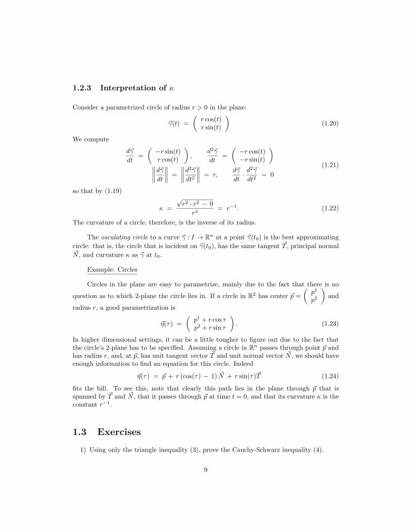
1.2.3 Interpretation of κ
Consider a parametrized circle of radius r > 0 in the plane:
~γ(t) =
(r cos(t)r sin(t)
)(1.20)
We compute
d~γ
dt=
(−r sin(t)r cos(t)
),
d2~γ
dt=
(−r cos(t)−r sin(t)
)∥∥∥∥d~γdt
∥∥∥∥ =
∥∥∥∥d2~γ
dt2
∥∥∥∥ = r,d~γ
dt· d
2~γ
dt2= 0
(1.21)
so that by (1.19)
κ =
√r2 · r2 − 0
r3= r−1. (1.22)
The curvature of a circle, therefore, is the inverse of its radius.
The osculating circle to a curve ~γ : I → Rn at a point ~γ(t0) is the best approximating
circle: that is, the circle that is incident on ~γ(t0), has the same tangent ~T , principal normal~N , and curvature κ as ~γ at t0.
Example: Circles
Circles in the plane are easy to parametrize, mainly due to the fact that there is no
question as to which 2-plane the circle lies in. If a circle in R2 has center ~p =
(p1
p2
)and
radius r, a good parametrization is
~η(τ) =
(p1 + r cos τp2 + r sin τ
). (1.23)
In higher dimensional settings, it can be a little tougher to figure out due to the fact thatthe circle’s 2-plane has to be specified. Assuming a circle in Rn passes through point ~p andhas radius r, and, at ~p, has unit tangent vector ~T and unit normal vector ~N , we should haveenough information to find an equation for this circle. Indeed
~η(τ) = ~p + r (cos(τ) − 1) ~N + r sin(τ)~T (1.24)
fits the bill. To see this, note that clearly this path lies in the plane through ~p that isspanned by ~T and ~N , that it passes through ~p at time t = 0, and that its curvature κ is theconstant r−1.
1.3 Exercises
1) Using only the triangle inequality (3), prove the Cauchy-Schwarz inequality (4).
9

2) Using only the triangle inequality for norms (3), prove the triangle inequality fordistances (6).
3) Consider the path ~γ : R → R3 given by γ1(t) = 23 t
32 , γ2(t) = sin(t), γ3(t) = cos(t).
Determine arclength s as a function of time, where s(0) = 0.
4) Reparametrize the path ~γ from problem (3) in terms of arclength.
5) Determine the best linear approximation to the given functions at the given points.
a) f : R→ R, f(x) = x2ex at x0 = 1
b) f : R2 → R, f(~x) = 2 + x1x2 +(x1)2
at ~x0 = (1,−1)T
c) ~f : R2 → R3, ~f(~x) =
(x1)2x2 + 1
x1x2
x1 + x2
at ~x0 =
(11
)
6) Determine the unit tangent ~T and the principal normal ~N for the following curves:
a) ~γ(t) =
(12 tt2
)b) ~η(t) = (cos(t), sin(t), t)
T
7) For curves (a) and (b) in problem (6), graph a portion of each curve, and graph ~T (t0)
and ~N(t0) at t0 = 1
8) Consider the plane curve ~γ(t) = (cos(t), 2 sin(t))T
.
a) Compute κ as a function of t.
b) Determine the equations of the osculating circles for t = 0 and t = π2 .
c) Sketch the graph of ~γ along with the osculating circles for t = 0 and t = π2 .
9) Consider the plane curve ~γ(t) = (t, t3)T ; its graph is the standard cubic. Determinethe osculating circle to the graph when t = 0.
10) If time is measured in seconds (s) and space is measured in meters (m), then what arethe units of geodesic curvature, κ?
No additional problems for 501 students this time.
10

Lecture 2 - Euler Curvature
Lecture given Tuesday Jan 21 — class shortened by snow.
2.1 Old calculus and new notation
2.1.1 Directional derivatives
In the new notational conventions, rows are parametrized with upper indices and columnswith lower indices. Let f : Rn → R be a real-valued function. Its partial derivatives aregiven the notation
f,i ,∂f
∂xi. (2.1)
so that it is natural to consider its gradient to be a row vector:
~∇f =
(∂f
∂x1,∂f
∂x2, . . . ,
∂f
∂xn
)= (f,1, f,2, . . . , f,n) (2.2)
Letting
~v =
v1
v2
...vn
(2.3)
be a vector, the rate of change of f in the ~v-direction is just the matrix product
(~∇f)
(~v) =(f,1, f,2, . . . , f,n)
v1
v2
...vn
=
n∑i=1
f,ivi. (2.4)
11

Consider another calculus problem. You are given a vector field
~F (x1, . . . , xn) =
F 1(x1, . . . , xn)...
Fn(x1, . . . , xn)
=
F 1
...Fn
(2.5)
and you wish to determine how the field is changing, at the point ~x in the direction ~v. Theanswer, of course, is to take the Jacobian of ~F
~∇~F =(F i,j)
=
F 1,1 F 1
,2 . . . F 1,n
F 2,1 F 2
,2 F 1,n
.... . .
...Fn,1 Fn,2 . . . Fn,n
(2.6)
where we have defined F i,j ,∂F i
∂xj , and to apply ~v = (v1, . . . , vn)T :
d~F
d~v= ~∇~F · ~v =
F 1,1 F 1
,2 . . . F 1,n
F 2,1 F 2
,2 F 1,n
.... . .
...Fn,1 Fn,2 . . . Fn,n
v1
v2
...vn
=
∑F 1,jv
j∑F 2,jv
j
...∑Fn,jv
j
(2.7)
A related question is the following. Given a function F : Rn → R and straight lineγ(t) = ~p+ ~vt in R2, what are the first and second derivatives of F γ? We have
dF
d~v= ~∇F ~v = (F,1, F,2, . . . , F,n)
v1
v2
...vn
=∑i
F,ivi (2.8)
The Hessian of F , namely
~∇2F = (F,ij) (2.9)
is a 2× 2 array whose indexing indicates it is a column-column matrix (instead of the usualrow-column matrix). This obviously can’t be drawn, but consider the usefulness of ourindexing scheme:
d
d~v
dF
d~v=
n∑i,j=1
F,ijvivj = ∇2F · ~v · ~v (2.10)
This is often denoted ∇2F (~v, ~v). In particular, any function F : R → R provides is with abilinear form:
∇2F (~v, ~w) =
n∑i,j=1
F,ijviwj . (2.11)
12

2.1.2 The Einstein sum convention
The Einstein sum convention consists of simply leaving off the sum sign, and wheneverrepeated upper and lower indices appear as a product, one knows to sum over them. So forinstance
dF
d~v= F,iv
i
∇2F (~v, ~w) = F,ijviwj .
(2.12)
and we can also write the inner product
〈~v, ~w〉 = ~vi ~wjδij (2.13)
Indeed the transpose of the column vector ~v = (vi) is the row vector (δijvj).
2.2 Curves on a surface
First consider the issue of unit-parametrized, straight-line paths in R2—these are determinedby a point ~p ∈ R2 and a direction, encoded by an angle θ. Then a unit-parametrized path
in R2 through ~p =
(p1
p2
)is given by
~µ(t) =
(p1 + t cos θp2 + t sin θ
). (2.14)
If further clarity is needed, we can explicitly index ~µ by its starting point ~p and direction θ:
~µ~p,θ(t) =
(p1 + t cos θp2 + t sin θ
). (2.15)
Now consider the graph of a function f(x1, x2). A path ~µ~p,θ(t) lifts to a graph on thesurface, given by
~γ~p,θ(t) =
p1 + t cos θp2 + t sin θ
f(p1 + t cos θ, p2 + t sin θ)
(2.16)
2.3 Euler’s notions of surface curvature
Let f(x1, x2) be some function, and let (p1, p2, f(p1, p2))T be a point on the graph, andconsider the family of paths through this point:
~γθ(t) =
p1 + t cos θp2 + t sin θ
f(p1 + t cos θ, p2 + t sin θ)
) (2.17)
13

(where we have left ~p implicit).
Now for each θ the curve γθ lies on the surface and has its own geodesic curvature.Each path passes through the point (p1, p2, f(p1, p2))T at time zero, so we can record thecurvature κ at that point. We define
κ(~p, θ) = curvature of the path ~γθ at time 0. (2.18)
Obviously κ will vary with θ. Fixing the point ~p and allowing θ to vary, we will find a largestand smallest curvature.
To arrive at Euler’s notion of surface curvature, we must also require that the principalnormal of these curves is also normal to the surface. When this is the case, the largest andsmallest curvatures are called the Eulerian principal curvatures κ1(~p) and κ2(~p). Specifically
κ1(~p) = supθ∈[0,π)
κ(~p, θ)
κ2(~p) = infθ∈[0,π)
κ(~p, θ).(2.19)
From these, Euler determined two measures of the curvature of a surface at a point:the Eulerian mean curvature and the Eulerian curvature, defined to be, respectively,
M =1
2(κ1 + κ2)
K = κ1κ2.(2.20)
2.4 Exercises
1) (Practice with notation.) Suppose the 3× 3 matrix (Aij) is given by Aij = −1 + i+ j.Also let
~v =
10−1
~w =
−110
(2.21)
a) Find the vector (Aijvj).
b) Express (δijvj) as a vector (is it a row or a column vector?).
c) Find the scalar Aijδikvjwk.
2) Consider the vector-valued function ~F : R3 → R3 given by
~F (x1, x2, x3) =
x1x2
12
((x1)2
+(x2)2
+ x2x3)
x1 − x2
(2.22)
14

a) Determine F 2,2 as a function of x1, x2 and x3.
b) At the point ~x = (1, 1, 1)T , how is the vector field changing in the direction~v = (
√3,√
3,√
3)T ?
3) Consider the surface given by the graph of f(x1, x2) = 12
((x1)2
+(x2)
2
10
). Simply
set ~p =
(00
)and determine the curvature κ(~p, θ) as a function of θ. Determine the
principal curvatures at this point.
Problems due Thursday Jan 30.
15

Lecture 3 - Euler Curvature,continued
Lecture given Thursday Jan 23.
3.1 A conceptual look at Euler curvature
Formal definition of principal curvature
Euler’s work was in surfaces in R3, so let’s spend a moment looking into the geometry here.
Given a point ~p ∈ R3 and a vector ~v based at ~p, how many planes exist that both passthrough ~p and contain the vector ~v? The answer, of course, is half a circle’s worth.
Now consider any (twice differentiable) surface Σ in R3, and let ~p be a point on Σ. At
~p, the surface itself has a normal vector ~N , so follows:
Now consider the family of planes that passes through ~p and that have a direction in
16

common with ~N . Two examples of such planes are as follows:
As you can see, each plane cuts out a curve that is both a plane-curve, and also a curveon the surface. At ~p itself, the tangent to each curve lies tangent to the surface, and becauseit is a plane curve, the normal to the curve must lie both along the plane and perpendicularto the unit tangent tangent, so each curve has as its normal the vector ~N , the normal tothe surface. Two examples of such curves are as follows:
17

Having fixed the point ~p and the normal vector ~N , we obtain a family of curves passingthrough ~p, and so that the principal normal of each curve at ~p is parallel to ~N . At p, eachcurve has a curvature κ. We make one more note: we define κ to be positive if the curve’sprincipal normal is ~N , and define κ to be negative if the curve’s principal normal is − ~N .
Now we can precisely define principal curvatures. Among all such curves passingthrough ~p, there will be a largest and a smallest curvature (possibly both negative!) .These are called the principal curvatures, and we label them
κ1(~p) and κ2(~p). (3.1)
This geometrical formulation has two main points. First, it is completely independentof any coordinate system. Thus there is no question of ambiguity arising from choosingdifferent origins, coordinate axes, or choosing spherical over rectangular coordinates, say.
The second point is even more significant. The reason for insisting that the principalnormals of the paths themselves are parallel to the surface’s normal is to unsure that, asmuch as possible, the paths are bending the way the surface is bending, and that the pathsare not bending in any way within the surface itself.
Procedure for computing principal curvatures
Somehow we have to parametrize the curves we obtained from the slicings described above.Since everything is coordinate-independent, the first step is to choose a propitious coordinatesystem: choose a system so that the point under consideration, ~p, is at the origin, and choosethe x1-x2 coordinate plane to be tangent to the surface at ~p.
In this case, the normal to the graph is simply the vector that points straight up
along the z-axis: ~N =
001
. The planes through the origin O that contain ~N can be
parametrized by the angle they make with the x1-axis, which we may call θ:
P (θ) = the 2-plane through O spanned by ~N =
001
and
cos θsin θ
0
= all linear combinations of
001
and
cos θsin θ
0
(3.2)
We can assume that the surface is given by the graph of a function f(x1, x2). The nextquestion is, how can we parametrize the path produced by the intersection of the graphx3 = f(x1, x2) and the plane P (θ)? If we call this path ~γθ, then
~γθ(t) =
t cos θt sin θ
f (t sin θ, t cos θ)
. (3.3)
18

3.2 Computation of curvatures, assuming ~∇f = 0
3.2.1 Geodesic curvatures of curves on a surface
Now let Σ be a surface in R3 given by the graph of a function, meaning
Σ =
x1
x2
f(x1, x2)
∣∣∣ ( x1
x2
)∈ Ω
(3.4)
where Ω is some domain in R2. We have assumed the coordinate system is chosen so thatf(0, 0) = 0 and ~∇f = ~0 The paths ~γθ(t), described in the previous section, are given by
~γθ(t) =
t cos θt sin θ
f (t cos θ, t sin θ)
(3.5)
The velocity and acceleration vectors are
d~γ
dt=
cos θsin θ
cos θ f,1 + sin θ f,2
d2~γ
dt2=
00
cos2 θ f,11 + 2 cos θ sin θ f,12 + sin2 θ f,22
(3.6)
and we compute∥∥∥∥d~γdt∥∥∥∥2
= 1 + (cos θ f,1 + sin θ f,2)2
∥∥∥∥d2~γ
dt2
∥∥∥∥2
=(cos2 θ f,11 + 2 cos θ sin θ f,12 + sin2 θ f,22
)2(d2~γ
dt2· d~γdt
)2
= (cos θ f,1 + sin θ f,2)2 (
cos2 θ f,11 + 2 cos θ sin θ f,12 + sin2 θ f,22
)2(3.7)
so that
κ =cos2 θ f,11 + 2 cos θ sin θ f,12 + sin2 θ f,22(
1 + (cos θ f,1 + sin θ f,2)2) 3
2
(3.8)
Notice that we dropped the absolute value. This is to account for the sign of κ, as discussedin the previous section. Finally, our assumption that ~∇f = ~0 forces f,1 = f,2 = 0, so weobtain
κ(θ) = cos2 θ f,11 + 2 cos θ sin θ f,12 + sin2 θ f,22 (3.9)
19

3.2.2 Principal curvatures
At our chosen point (the origin), we now have κ as a function of θ being
κ(θ) = cos2 θ f11 + 2 cos θ sin θ f12 + sin2 θ f22. (3.10)
We want to extremize κ, so we take a derivative and set to zero:
0 =dκ
dθ
= −2 cos θ sin θ f11 + 2(cos2 θ − sin2 θ
)f12 + 2 cos θ sin θ f22
= − sin(2θ) (f11 − f22) + 2 cos(2θ)f12
(3.11)
We obtain
cot(2θ) =f11 − f22
2f12. (3.12)
Noting that we must accept all solutions for θ ∈ [0, π) so that 2θ may be in [0, 2π), wetherefore obtain two solutions for θ, characterized by
sin(2θ) = ± 2f12√(f11 − f22)
2+ 4 (f12)
2
cos(2θ) = ± f11 − f22√(f11 − f22)
2+ 4 (f12)
2.
(3.13)
From the half-angle formulas we get
sin2 θ =1− cos(2θ)
2=∓ (f11 − f22) +
√(f11 − f22)
2+ 4 (f12)
2
2
√(f11 − f22)
2+ 4 (f12)
2
cos2 θ =1 + cos(2θ)
2=± (f11 − f22) +
√(f11 − f22)
2+ 4 (f12)
2
2
√(f11 − f22)
2+ 4 (f12)
2
(3.14)
Putting this in to (3.10) we find that the two principal curvatures are
κ1 =f11 + f22 +
√(f11 − f22)
2+ 4 (f12)
2
2
κ2 =f11 + f22 −
√(f11 − f22)
2+ 4 (f12)
2
2.
(3.15)
3.2.3 Euler’s first theorem and Gauss’ second derivative test
Theorem 3.2.1 (Euler, 1760) The two paths that represent the principal curvatures of asurface Σ at any point ~p intersect at right angles.
20
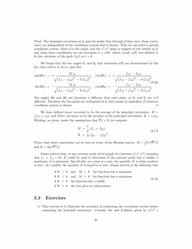
Proof. The principal curvatures at ~p, and the paths that through ~p that carry those curva-tures, are independent of the coordinate system that is chosen. Thus we can select a specialcoordinate system, where ~p is the origin, and the x1-x2 plane is tangent to the surface at ~p,and using these coordinates we can extremize κ = κ(θ), where, recall, κ(θ) was defined tobe the curvature of the path ~γθ(t) at t = 0.
We found that the two angles θ1 and θ2 that extremize κ(θ) are characterized by thefact that each is in [0, π), and that
sin(2θ1) = +2f,12√
(f,11 − f,22)2 − 4 (f,12)
2, cos(2θ1) = +
f,11 − f,22√(f,11 − f,22)
2 − 4 (f,12)2
sin(2θ2) = − 2f,12√(f,11 − f,22)
2 − 4 (f,12)2, cos(2θ2) = − f,11 − f,22√
(f,11 − f,22)2 − 4 (f,12)
2
(3.16)
The angles 2θ1 and 2θ2 are therefore π different from each other, so θ1 and θ2 are π/2different. Therefore the two paths are orthogonal at ~p, and remain so regardless of whatevercoordinate system is chosen.
We have defined mean curvature to be the average of the principal curvatures: M =12 (κ1 + κ2), and Euler curvature to be the product of the principal curvatures: K = κ1κ2.
Working, as above, under the assumption that ~∇f = 0, we compute
M =1
2(f11 + f22)
K = f11f22 − (f12)2.
(3.17)
Notice that these expressions can be seen in terms of the Hessian matrix: M = 12Tr(
~∇2f)
and K = det(~∇2f).
Gauss noticed that, at any extreme point of the graph of a function f(x1, x2) (meaningthat f,1 = f,2 = 0), K could be used to determine if the extreme point was a saddle, amaximum, or a minimum. Specifically, at a max or a min, the quantity K is either positiveor zero. At a saddle, the quantity K is negative or zero. Gauss arrived at the following rule:
if K > 0 and M > 0 the function has a minimum
if K > 0 and M < 0 the function has a maximum
if K < 0 the function has a saddle
if K = 0 the test gives no information.
(3.18)
3.3 Exercises
1) This exercise is to illustrate the necessity of rechoosing the coordinate system beforecomputing the principal curvatures. Consider the unit 2-sphere, given by (x1)2 +
21

(x2)2 + (x3)2 = 1 in x1, x2, x3 coordinates. Let ~p =(
1√2, 0, 1√
2
)T. We can consider
the upper-half sphere to be the graph of f(x1, x2) =
√1 − (x1)
2 − (x2)2. Let ~γθ be
the path, passing through ~p at time t = 0 whose osculating plane is parallel to thex3-axis and makes the angle θ with the x1-axis. This path is given by
~γθ(t) =
1√2
+ t cos θ
t sin θ
f(
1√2
+ t cos θ, t sin θ) . (3.19)
a) Find the curvature κ of the path ~γθ, as a function of θ.
b) What is the maximum and the minimum of the function κ(θ) from (a)?
c) For the unit sphere, we know that K = 1 and M = 1 (see problem (2)). Howeverif you were to find κ1 and κ2 from (b), you would compute larger values for both.Explain why; especially explain why the spurious values from this problem arelarger and not smaller than the true values.
2) Consider the sphere of problem (1), along with the point ~p =(
1√2, 0, 1√
2
)T. Go
through the whole process of determining the mean and Eulerian curvatures at ~p,including re-choosing the coordinate system, compute κ as a function of θ, and so on.You must describe the method step by step, but if you use some common sense andyour basic knowledge of spheres, this won’t be a difficult problem. Was there anythingspecial about the point ~p?
3) Consider the surface obtained by graphing f(x1, x2) = x1x2. Find K and M at thepoint (0, 0, 0)T on the surface. Explain why κ1 and κ2 have opposite signs.
4) Given our computations (3.10) and (3.13), verify formula (3.15).
5)* Given any n × n symmetric matrix A = (aij), prove that its eigenvalues are real andnon-degenerate, and it has orthogonal eigenvectors.
6)* Euclidean space Rn is the n-dimensional vector space with distance measured by thePythagorean theorem, infinitesimally expressed by
ds =
√(dx1)
2+ . . . + (dxn)
2. (3.20)
Now define Rn,k to be the (n + k)-dimensional vector space with distance measured(infinitesimally) by
ds =
√(dx1)
2+ . . . + (dxn)
2 − (dxn+1)2 − . . . − (dxn+k)
2. (3.21)
In particular, the spaces R1,k (or sometimes Rn,1) are the Lorentzian vector spaces ofspecial relativity. Sketch the following paths, and compute their lengths as a functionof t
22

a) ~γ(t) =
(t1
)in R1,1
b) ~γ(t) =
(tt
)in R1,1
c) ~γε(t) =
(εtt
)(as a function of ε and t) in R1,1
d) ~γ(t) =
tcos(t)sin(t)
, t ∈ [0, t0], any t0, in R1,2
Exercises marked with a “∗” are for 501 students.
Problems due Thursday Jan 30.
23
Lecture 4 - Euler’s Theorem.The Gauss Map.
4.1 Aside: Symmetric 2× 2 matrices
Let A be a matrix of the form (a cc b
). (4.1)
Any symmetric matrix has real, orthogonal eigenvalues. Further, computation reveals thatthe two eigenvectors and corresponding eigenvectors are
λ1 =a+ b+
√(a− b)2 + 4c2
2, ~v1 =
2c
−a+ b+√
(a− b)2 + 4c2
λ2 =
a+ b−√
(a− b)2 + 4c2
2, ~v2 =
2c
−a+ b−√
(a− b)2 + 4c2
(4.2)
4.2 Euler’s Second Theorem
Consider again the surface Σ, with a point ~p ∈ Σ, and a choice of coordinate systems thatmakes ~p the origin with the x3-axis parallel to the normal ~N at ~p.
At ~p denote the principal directions by ~V1 and ~V2. These are the initial velocities ofthe paths that carry the principal curvatures. From (3.14) we easily compute
~V1 =
2f12
− (f11 − f22) +
√(f11 − f22)
2+ 4 (f12)
2
~V2 =
2f12
− (f11 − f22)−√
(f11 − f22)2
+ 4 (f12)2
(4.3)
24
which of course are the eigenvectors of the Hessian ~∇2f . We make a final computationbefore wrapping things up. Consider a path along the graph through ~p that makes an angleof ϕ with the ~V1-direction. Then using (3.15)
cos2 ϕκ1 + sin2 ϕκ2 =f11 + f22 + cos(2ϕ)
√(f11 − f22)
2+ 4 (f12)
2
2(4.4)
Recall that we used θ to denote the angle with respect to the x1-axis in our special coordinatesystem. Now ϕ and θ are related by an offset that we shall call θ1, which is just the angle~V1 makes with the x1-axis, whose sine and cosine are given by (3.14). We compute
cos(2ϕ) = cos(2θ − 2θ1)
= cos(2θ) cos(2θ1) + sin(2θ) sin(2θ1)
= cos(2θ)f11 − f22√
(f11 − f22)2
+ 2 (f12)2
+ sin(2θ)2f12√
(f11 − f22)2
+ 2 (f12)2
(4.5)
so that
cos2 ϕκ1 + sin2 ϕκ2 =f11 + f22 + cos(2θ) (f11 − f22) − 2 sin(2θ) f12
2
=1 + cos(2θ)
2f11 +
1− cos(2θ)
2f22 + sin(2θ) f12
= cos2 θ f11 + sin(2θ) f12 + sin2 θ f22 = κ
(4.6)
This is the Euler curvature formula, which is Euler’s second theorem.
Theorem 4.2.1 (Euler, 1760) Let κ1 and κ2 be the principal curvatures at a point ~p
on a surface, and let ~V1, ~V2 be the corresponding principal directions. Then ~V1 and ~V2
are orthogonal, and the direction along the surface that makes an angle of ϕ with ~V1 hascurvature
κ(ϕ) = cos2 (ϕ) κ1 + sin2 (ϕ) κ2. (4.7)
4.3 Some geometry of level-sets
4.3.1 Gauss’ idea
Recall the Frenet formulas
d
ds
~T~N~B
=
0 κ 0−κ 0 τ0 −τ 0
~T~N~B
(4.8)
25
In Euler’s methodology, the curves used to study the surface are also plane curves, so τ = 0.This means that
d~T
ds= κ ~N
d ~N
ds= −κ~T .
(4.9)
for each of the curves. So instead of studying the tangent vectors of these paths, we couldstudy the way the normal vectors change. However these normal vectors are chosen tocoincide with the normal to the surface itself.
Gauss’ idea was to study the normal vector to the surface itself, without the compli-cation of having to choose specific curves on the surface. Gauss’ methods, which we willspend the next few lectures on, have the added advantage of being easily applicable in higherdimension.
4.3.2 Level-sets and normals
We have been considering surfaces given by the graph of a function, but in the study ofgeometry it is often better to study level sets of functions. This allows us to study objectsthat cannot be expressed as the graph of anything. For instance, consider the objects
F (x1, x2, x3) =((x1)2
+(x2)2
+(x3)2)
, F (x1, x2, x3) = c
F (x1, x2, x3) =((x1)2
+(x2)2
+(x3)2 − 1
) (x1 + x2 − x3
), F (x1, x2, x3) = 0.
(4.10)
The first is the sphere of radius√c, and the second is the union of sphere of radius 1 with
the plane x3 = x1 + x2.
A hypersurface in Rn will, from now on, be considered to be a level-set of the formF = 0 for some function F : Rn → R. The gradient of a function F is always orthogonal toits level-sets (as long as |~∇F | is non-zero), so we have the two unit normals:
n = ±~∇F∣∣∣~∇F ∣∣∣ . (4.11)
A surface F = 0 is called non-singular at ~p = (x1, . . . , xn)T if (in addition to F (~p) = 0) we
have ~∇F (~p) 6= ~0. A point on the surface F = 0 is singular if also ~∇F = ~0. Note that the
system of equations F = 0 and ~∇F = ~0 is overdetermined, meaning you usually can’t findany critical points. This is a primitive version of Sard’s theorem.
26

4.4 The Gauss Map
Let Mn−1 be the (n− 1)-dimensional surface in Rn given by a non-singular level set F = 0,where F : Rn → R. The Gauss map, G, is simply the map that sends each point p ∈Mn−1
to the normal vector at that point. Since any normal vector lies on the sphere Sn−1 ⊂ Rn,this map can be thought of as a map
G : Mn−1 −→ Sn−1. (4.12)
We have a formula for the unit normal to a surface, provided the surface is given by thelevel-set F = 0. Let’s look at a few examples of the Gauss map for surfaces Σ ∈ R3.
Example: The Gauss map for the flat 2-plane
Choosing Σ ⊂ R3 to be the x1-x2 plane, the normal vector field ~N is the constant
~N = (0, 0, 1) . (4.13)
The image of the Gauss map is therefore simply the north pole on the 2-sphere.
Example: The Gauss map for the cylinder.
Consider the function F (x1, x2, x3) =(x1)2
+(x2)2 − 1. The level-set
Σ = (x1, x2, x3)T | F (x1, x2, x3) = 0 (4.14)
is simply the cylinder of radius 1 that is translated up and down the x3-axis. If ~p =(p1, p2, p3)T ∈ Σ, then the unit normal is
∇F|∇F |
(p1, p2, p3) =
(2p1, 2p2, 0
)2
√(p1)
2+ (p2)
2=(p1, p2
). (4.15)
The image of the Gauss map is therefore the equator of the unit sphere.
Example: The Gauss map for the sphere of radius r.
The point ~p = (p1, p2, p3)T is on the sphere of radius r if(p1)2
+(p2)2
+(p3)2
= r2.The unit normal at ~p is quite simply ~p/|~p|. The image of the Gauss map is therefore theentire sphere.
Indeed, the Gauss map on the unit 2-sphere can be considered the identity map.
Example: The Gauss map for a paraboloid.
Let F (x1, x2, x3) = x3 − 12
((x1)2
+(x2)2)
, and set Σ = F = 0. The unit normal is
∇F|∇F |
=(−x1,−x2, 1)√
1 + (x1)2 + (x2)2=
(−x1,−x2, 1)√1 + 2x3
(4.16)
27
Notice that the inner product⟨
(0, 0, 1), ∇F|∇F |
⟩> 0 at all times. This means that the angle
between the unit normal and the vertical vector is always acute, so the image of the Gaussmap is within the upper hemisphere. It is easy to see that the image in indeed the entire(open) upper hemisphere.
4.5 Exercises
1) Verify the formulas in (4.2). Examine the cases that a = b and that c = 0.
2) Consider the case of “hypersurfaces” in R2 (that is, curves). Specifically, consider thelevel sets Fc(x
1, x2) = 0, where Fc is the cubic, parametrized by c, given by:
Fc(x1, x2) = (x2)2 − 1
3(x1)3 + x1 − c. (4.17)
For generic c, determine all singular points of the curve. Graph several representativecurves, and explicitly label all singular points.
3) Consider the family of surfaces in R3, parametrized by c, given by the quadratic
polynomials Fc(x1, x2, x3) = −
(x1)2−(x2
)2+(x3)2
+c. Sketch several representativesurfaces for c in the range, say, [−2, 2]. For each c, determine all singular points andlabel them on your graph.
*4) Prove that mean curvature is not just the mean of the principal curvatures, but themean of all curvatures as θ varies through the entire circle of directions.
**5) Can Euler curvature can be expressed as a total integral for θ ∈ [0, 2π), as you ex-pressed mean curvature in (3)?
6) Consider the parabola in R2; this is given by the zero-set of F = −x2 +(x1)2
. Sketchthe image of the Gauss map, and label, on S1, the images of the points (0, 0)T , (1, 1)T
and (−1, 1)T .
7) Compute, explicitly, the Gauss map G of Σ = F = 0, where F (x1, x2, x3) =
x3 − 12
((x1)2 − (x2
)2). Label the images of the points (0, 0, 0)T , (1, 1, 0)T , and
(√
3, 1, 1)T ?. As a set, what is the image G(Σ)?
*8) Let Σ be a surface in R3 that is the graph of a (twice continuously differentiable)function. Prove that the image of the Gauss map is contained in a hemisphere of S2.
Exercises marked with a “∗” are for 501 students. Exercises marked with a “∗∗” areoptional.
Problems due Thursday Feb 6.
28
Lecture 5 - The First andSecond Fundamental Forms
5.1 Gauss’ definition of curvature
If Σ2 is a surface in R3, the Gauss map G : Σ2 → R3 distorts the shape of Σ rather severely.In particular, consider a domain R ⊂ Σ, and consider how it maps to S2. Its image is G (R).Now consider a point p ∈ Σ, and consider all domains Rp in Σ that contain p. The Gaussiancurvature of Σ at p, denoted KG, was defined by Gauss to be
KG(p) = limRp→p
Area(G(Rp))Area(Rp)
(5.1)
Now this definition is not rigorous, because exactly what is meant by limRp→p is problem-atic. Possibly a clear notion of this limit can be obtained, but it would require an involvedargument to prove that the limit doesn’t depend on the way that the domains Rp shrinkdown to the set p. Further below, we take a more modern approach to all this.
5.2 Tangent Spaces and the First Fundamental Form
Let Σ be the hyper-surface in Rn given by F (x1, . . . , xn) = 0. A point p ∈ Σ is said to
be a singular point provided ~∇F = ~0. If the point p is non-singular, then it is possible todetermine a tangent space to Σ at p. This is denoted TpΣ, and defined to be the followingvector space:
TpΣ ,
vectors ~v based at p such that⟨~V , ~N
⟩= 0
. (5.2)
Gauss defined a bilinear form, the first fundamental form to be simply the restriction of theinner product to the tangent space:
I (~v, ~w) = 〈~v, ~w〉 , provided ~v, ~w ∈ TpΣ. (5.3)
Often the form I is denoted by g.
29

5.3 The Second Fundamental Form
The Gauss map is a map that sends any non-singular surface Σ ∈ Rn to the unit sphereSn−1. Gauss wants to look at how regions in Σ map to regions on Sn−1, but his methodis not rigorously defined. Still, if we want to look at the infinitesimal way that areas aredistorted, we look at the Jacobian of the Gauss map. This is the matrix
~∇
~∇F∣∣∣~∇F ∣∣∣ =
((Fi|∇F |
)j
)ni,j=1
(5.4)
This Jacobian is useful in a number of ways. For instance if you want to know how the
normal vector~∇F|~∇F |
is changing in the direction ~v, you simply compute
~∇
~∇F∣∣∣~∇F ∣∣∣ (~v) . (5.5)
We define the second fundamental form to be this Jacobian, restricted to the tangentspace at p ∈ Σ:
II , ~∇
~∇F∣∣∣~∇F ∣∣∣∣∣∣∣∣∣
TpΣ
II (~v, ~w) = ∇(∇F|∇F |
)(~v, ~w) , for ~v, ~w ∈ TpM
(5.6)
In coordinates, after letting ~v = (vi) and ~w = (wi) be vectors in TpΣ, we have
II (~v, ~w) = ∇(∇F|∇F |
)(~v, ~w)
=
F,i∣∣∣~∇F ∣∣∣,j
vi wj
=∂
∂xi
1∣∣∣~∇F ∣∣∣ ∂F∂xj vi wj
(5.7)
5.4 Examples
Consider the surface Σ ⊂ R3 given by F = 0 where F (x1, x2, x3) =(x1)2
+(x2)2−(x3
)2−1.
Assuming p ∈ Σ, we will determine ~N(p), a basis for TpΣ, and the two fundamental formsexpressed in this basis.
30

The normal vector is
~N =
(2x1, 2x2, −2x3
)√4 (x1)
2+ 4 (x2)
2+ 4 (x3)
2
=
(x1, x2, −x3
)√(x1)
2+ (x2)
2+ (x3)
2.
(5.8)
At the point p = (p1, p2, p3)T , we can simplify this (slightly) to
~N(p) =
(x1, x2, −x3
)√1 + 2 (x3)
2(5.9)
Let ~Z = (0, 0, 1) be the unit vector in the x3-direction, and let ~R = (−x2, x1, 0) be the
radial vector field. At the moment, there is no reason to believe that ~Z, ~R ∈ TpΣ. But these
vectors are independent of ~N , so we can apply a normalization process. Set
~v1(p) = ~Z −
⟨~Z, ~N
⟩⟨~N, ~N
⟩ ~N
= (0, 0, 1) −⟨(0, 0, 1), (p1, p2,−p3)
⟩√1 + 2 (p3)
2·(p1, p2, −p3
)√1 + 2 (p3)
2
=
(p1p3, p2p3, 1 +
(p3)2)
1 + 2 (p3)2
(5.10)
and
~v2(p) = ~R −
⟨~R, ~N
⟩⟨~N, ~N
⟩ ~N
=(−p2, p1, 0
)−⟨(−p2, p1, 0), (p1, p2,−p3)
⟩√1 + 2 (p3)
2·(p1, p2, −p3
)√1 + 2 (p3)
2
=(−p2, p1, 0
)(5.11)
(so it turns out that ~v2 was orthogonal to ~N after all). Now the two vectors ~v1 and ~v2 are
orthogonal to ~N (and indeed are orthogonal to each other), so that
TpΣ = span ~v1, ~v2 . (5.12)
31

In this basis, we compute the first fundamental form:
I(p) =
(I11 I12
I21 I22
)=
(〈~v1, ~v1〉 〈~v1, ~v2〉〈~v2, ~v1〉 〈~v2, ~v2〉
)
=
1+(p3)
2
1+2(p3)20
0 1 +(p3)2 (5.13)
For the second fundamental form, the easiest thing to do is to compute ∇(∇F/|∇F |)as a 3 × 3 matrix in the variables x1, x2, and x3, and then evaluate at ~v1 and ~V2. Wecompute
∇(∇F|∇F |
)=
∂∂x1
(1|∇F |
∂F∂x1
)∂∂x1
(1|∇F |
∂F∂x2
)∂∂x1
(1|∇F |
∂F∂x3
)∂∂x2
(1|∇F |
∂F∂x1
)∂∂x2
(1|∇F |
∂F∂x2
)∂∂x2
(1|∇F |
∂F∂x3
)∂∂x3
(1|∇F |
∂F∂x1
)∂∂x3
(1|∇F |
∂F∂x2
)∂∂x3
(1|∇F |
∂F∂x3
)
(5.14)
Using (5.8) (NOT (5.9)), we compute
∇(∇F|∇F |
)= 1
((x1)2+(x2)2+(x3)2)32
(x2)2
+(x3)2 −x1 x2 x1 x3
−x1 x2(x1)2
+(x3)2
x2 x3
−x1 x3 −x2 x3 −(x1)2 − (x2
)2
(5.15)
As an aside, notice that this matrix is not symmetric.
Now we can compute II. We have
IIp =
(IIp (~v1, ~v1) IIp (~v1, ~v2)IIp (~v2, ~v1) IIp (~v2, ~v2)
)
=
− 1+(p3)2
(1+2(p3)2)5/2 0
0 1+(p3)2
(1+2(p3)2)1/2
(5.16)
5.5 Exercises
1) (First fundamental form) Consider the surface given by F = 0 and x3 > 0 where
F (x1, x2, x3) = −(x1)2 − (x2
)2+(x3)2 − 1. (5.17)
32

Determine a basis ~v1, ~v2 for TpΣ, where p = (p1, p2, p3)T . In your basis, determine
the matrix I. (Hint: Let ~X = (1, 0, 0) and ~Y = (0, 1, 0), and apply a normalizationprocess.)
2) (Second fundamental form) Consider the surface from problem (1). In your chosenbasis, and at the point p = (0, 0, 1)T , compute II as a 2× 2 matrix.
3) Let Σ be a hypersurface given as the graph of some function x3 = f(x1, x2). Compute~N , and determine a basis for TpΣ at p = (p1, p2, p3)T .
*4) In the situation of problem (3), compute ∇(∇F|∇F |
)in components.
5) (Parametriations) A third way to describe surfaces is via parametrizations. A parametrizedsurface in Rn is a surface Σ ⊂ Rn along with a map P : Ω→ Σ where Ω is a domainin R2 that is differntiable, one-to-one and onto.
a) Graph the surface
P : R2 −→ R3
P (s, t) =
s2 + t2
st
.(5.18)
*b) What kind of parametrized surface is this?
P : [0, 2π)× [0, 2π) −→ Σ ⊂ R4
P (s, t) =
1√2
cos(t)1√2
sin(t)1√2
cos(s)1√2
sin(s)
.(5.19)
Also, verify that Σ is contained within the unit sphere S3 ⊂ R4.
6) (Coordinate Charts) If Σ is some surface in Rn and Ω is some domain in Σ, then acoordinate chart is a map S : Ω→ R2 that is differentiable and one-to-one (but needn’tbe onto). If p ∈ Σ, then the coordinates of p are the two coordinates of S(p). Let
Σ be the unit sphere S2 ⊂ R3, given by(x1)2
+(x2)2
+(x3)2 − 1 = 0. For a point
p = (p1, p2, p3) ∈ S3, define
S(p) =
x1
√1−x3
x2√
1−x3
(5.20)
What are the coordinates of the following points?
p =
1/√
2
1/√
20
, q =
00−1
, r =
100
, s =
1/√
3
1/√
3
1/√
3
(5.21)
33

*7) Under what conditions is it true that II = ∇2F|∇F |? That II = ∇2F? In the case of a
graph of a function: F (x1, x2, x3) = x3 − f(x1, x2), what does II = ∇2F|∇F | at a point
(x1, x2, f(x1, x2))T imply about f at the point (x1, x2)?
Exercises marked with a “∗” are for 501 students.
Problems due Thursday Feb 6.
34

Lecture 6 - Gaussian Curvature
Lecture from Thursday Feb 6, 2012.
6.1 Identity and transpose operators
Symbolically, all of δji , δij and δij are the same. However, consider a vector ~v = (vi), whichis a column vector. The vector (δijv
j) is simply ~v again. But (δijvj) is not ~v but rather ~vT .
Similarly (f,jδij) is a column vector, instead of a row vector.
If A = (Aij) is a matrix, we can transpose either of its indices if we wish: we coulddefine
Bij = Akj δik (6.1)
or
Cij = Aikδkj . (6.2)
We briefly consider the case of symmetric matrices; these are matrices so that A = AT .Symbolically, it is true that Aij = Aji . But this is weird: we are equating symbols withmixed-up indices. It is notationally correct to write
Aij = δikδljAlk (6.3)
which means the same thing.
6.2 Coordinate systems
Let xini=1 be a coordiate system on En. A basic fact is that each of the xi is a function.This means that, if yana=1 is a second coordinate system, then we can take the derivativeof any of the xi with respect to any of the ya.
Example (Polar and rectangular coordinates on E2.)
35

Let x1, x2 be orthonormal coordinates on 2-dimensional Euclidean space. Let
y1 =
√(x1)
2+ (x2)
2y2 = tan−1
(x1/x2
). (6.4)
However we can also define the original coordinates in terms of the new coordinates:
x1 = y1 cos(y2)
x2 = y1 sin(y2). (6.5)
We have the transition matrices
(∂ya
∂xi
)=
∂y1
∂x1∂y1
∂x2
∂y2
∂x1∂y2
∂x2
=
x1√
(x1)2 + (x2)2x2√
(x2)2 + (x2)2
−x2
(x1)2 + (x2)2x1
(x1)2 + (x2)2
(6.6)
and
(∂xi
∂ya
)=
∂x1
∂y1∂x1
∂y2
∂x2
∂y1∂x2
∂y2
=
cos(y2) −y1 sin(y2)
sin(y2)
y1 cos(y2)
(6.7)
Now consider the product:
(∂ya
∂xi
)·(∂xi
∂ya
)=
∂y1
∂x1∂y1
∂x2
∂y2
∂x1∂y2
∂x2
∂x1
∂y1∂x1
∂y2
∂x2
∂y1∂x2
∂y2
=
x1 cos(y2)+x2 sin(y2)√
(x1)2 + (x2)2−x1y1 sin(y2)+x2y1 cos(y2)√
(x1)2 + (x2)2
−x2 cos(y2)+x1 sin(y2)
(x1)2 + (x2)2x1y1 cos(y2)+x2y1 sin(y2)
(x1)2 + (x2)2
(6.8)
Now since cos(y2) = x1/√
(x1)2 + (x2)2 and sin(y2) = x2/√
(x1)2 + (x2)2, we compute(∂ya
∂xi
)·(∂xi
∂ya
)=
(1 00 1
)(6.9)
Is this an accident? No.
36

Theorem 6.2.1 Let xini=1 and yana=1 be two coordinate systems. Then
δij =∂xi
∂ya∂ya
∂xjand
δab =∂ya
∂xi∂xi
∂yb.
(6.10)
Proof. By the chain rule we have
∂
∂xj=
∂ya
∂xj∂
∂ya(6.11)
Noting that ∂xi
∂xj = δij , we have
δij =∂xi
∂xj=
∂ya
∂xj∂xi
∂ya(6.12)
which proves the first assertion. The second assertion can be shown likewise.
6.3 Gaussian Curvature
Recall Gauss’ definition of curvature
KG(p) “ = ” limR→p
Area (G(R))
Area (R)(6.13)
where the limit is, in principal, taken as the open regions R get smaller and smaller, con-verging on the point p. Of course, this is not rigorous. We formally define
KG(p) =det IIpdet Ip
. (6.14)
The determinants are taken after a basis ~v1, ~v2 is chosen at p ∈ TpΣ. To be specific, thematrices are
I =
(I11 I12
I21 I22
)=
(〈~v1, ~v1〉 〈~v1, ~v2〉〈~v2, ~v1〉 〈~v2, ~v2〉
)
II =
(II11 II12
II21 II22
)=
∇( ∇F|∇F |) (~v1, ~v1) ∇(∇F|∇F |
)(~v1, ~v2)
∇(∇F|∇F |
)(~v2, ~v1) ∇
(∇F|∇F |
)(~v2, ~v2)
(6.15)
6.4 Exercises
We didn’t get through a lot this time, so we have only a few workbook-style exercises.
37

1) (Coordinates) Let x1, x2 be the standard coordinates on R2. Define new coordinates
y1 =(x1)2 − (x2
)2y2 = x1 − x2.
(6.16)
a) Determine x1 and x2 as functions of y1 and y2.
b) Make a sketch of the coordinate system y1, y2. Label the points (0, 0)T ), (1, 1)T
and (−1,−2)T (given in y-coordinates). Sketch the graph of the function
y2 = 3y1 + 1.
c) Compute the matrices (∂xi
∂ya
)and
(∂ya
∂xi
)(6.17)
and prove that they are inverses of each other.
2) Assume that the coordinate systems xi and yi are mutually orthogonal; this meansthat the matrices (
∂xi
∂ya
)ni,a=1
and
(∂ya
∂xi
)ni,a=1
(6.18)
are not just inverses (which we proved is always the case), but that they are transposes.Prove that
δab∂xi
∂ya∂xj
∂yb= δij . (6.19)
To get full credit, you must use the correct symbolic calculus as outlined in Section 1.
3) Consider F : R3 → R given by F (x1, x2, x3) =(x1)2
+(x2)2
+(x3)2 − 1, and let Σ
be the surface F = 0. Let ~X = (1, 0, 0)T and ~Y = (0, 1, 0)T be vector fields on R3.
a) Given any point (p1, p2, p3)T ∈ Σ, find ~N .
b) At each point of Σ, project ~X and ~Y onto the tangent space of Σ (there is a basicformula for this). Call the new vectors ~v1 and ~v2.
c) Show that ~v1 and ~v2 span TpΣ, except for when p is on the “equator” (theintersection of Σ and the x1-x2 plane).
d) Let p ∈ Σ be any point that’s not on the equator. In the ~v1, ~v2 basis, show that
Ip =
(1− (x1)2 −x1x2
−x1x2 1− (x2)2
), (6.20)
and show that, as expected, Ip is singular when p is on the equator.
4) Let F and Σ be as in (3).
38

a) Compute ∇(|∇F |−1∇F
)as a 3× 3 matrix. Show that it is singular.
b) In the basis from (3b), compute II as a matrix.
c) Prove that KG(p) = 1.
*5) On tangent spaces in Rn,k, we use the inner product
〈~v, ~w〉 = ~vT In,k ~w (6.21)
where
In,k =
1 0. . .
1−1
. . .
0 −1
(6.22)
where there are 0’s in every entry except along the main diagonal, where there are nmany 1’s followed by k many −1’s. Likewise, recall the Rn,k Pythagorean theorem:in standard coordinates, if p = (p1, . . . , pn+k)T is a point, then the distance from theorigin to p is
dist(O, p) =
√(p1)
2+ · · ·+ (pn)
2 − (pn+1)2 − · · · − (pn+k)
2. (6.23)
The set of all points p ∈ R1,2 that have distance 1 to the origin is a surface of twocomponents; the component with x1 > 0 is known as the unit pseudosphere. Make asketch of this pseudosphere. Prove that its first fundamental form is in fact positivedefinite.
Problems due Thursday 2/13
39
Lecture 7 - Gaussian andEulerian Curvature
Lecture from Tuesday Feb 11, 2012
7.1 Bases and Change of Basis
7.1.1 Bases
Given an n-dimensional vector space Vn, a basis is normally indexed with lower indices:
~e1, . . . , ~en. (7.1)
For instance, we could have the standard basis when Vn = Rn
~ei =
0...1...0
(7.2)
where the 1 is in the ith position. Then a vector ~v can be expressed as a linear combinationof the basis vectors:
~v = viei =
v1
...vn
(7.3)
40
7.1.2 Change of basis
Assume ~eini=1 and ~fini=1 are two bases for Vn. We have change of basis symbols
~ej = Aij~fi
~fj = Bij~vi.(7.4)
We have that matrices (Aij) and (Bij) are inverses of one another: AijBjk = δik. This is simple
to prove:
~ei = Aji~fj = AjiB
kj ~ek. (7.5)
But, because ~ej is a basis, the only linear combination of the ~ej that gives ~ei is given
by ~ei = δki ~ek. Therefore AjiBkj = δki .
7.2 Gaussian curvature and change of basis
Recall the first and second fundamental forms:
I = 〈·, ·〉∣∣TpΣ
II = ∇(∇F|∇F |
)∣∣∣∣TpΣ
(7.6)
After a basis ~v1, ~v2 is chosen for TpΣ, we can express these as matrices:
I =
(I11 I12
I21 I22
)=
(〈~v1, ~v1〉 〈~v1, ~v2〉〈~v2, ~v1〉 〈~v2, ~v2〉
)
II =
(II11 II12
II21 II22
)=
∇( ∇F|∇F |) (~v1, ~v1) ∇(∇F|∇F |
)(~v1, ~v2)
∇(∇F|∇F |
)(~v2, ~v1) ∇
(∇F|∇F |
)(~v2, ~v2)
.
(7.7)
After doing all this, the Gaussian curvature KG and the Gaussiam mean curvature MG aredefined as follows:
KG = det(I−1II
)=
det(II)
det(I)
MG =1
2Tr(I−1II
).
(7.8)
A glaring issue is in the choice of basis: if we choose a different basis for TpΣ, the matrixrepresentations of II and I are obviously not the same. So aren’t the values of KG and MG
affected? The answer is no.
Theorem 7.2.1 The values of KG and MG are independent of the basis that is chosen.
41

Proof. Let ~v1, ~v2 and ~w1, ~w2 be two different bases for TpΣ, with transitions
~vi = Aji ~wj
~wi = Bji~vj(7.9)
Let
I =
(I11 I12
I21 I22
)II =
(II11 II12
II21 II22
)(7.10)
I ′ =
(I ′11 I ′12
I ′21 I ′22
)II ′ =
(II ′11 II ′12
II ′21 II ′22
)(7.11)
be the first and second fundamental forms expressed in the two bases. Explicitly, let
Iij = 〈~vi, ~vj〉 IIij = ∇(∇F|∇F |
)(~vi, ~vj)
I ′ij = 〈~wi, ~wj〉 II ′ij = ∇(∇F|∇F |
)(~wi, ~wj).
(7.12)
Now both of these forms are bilinear, so we compute
Iij = 〈~vi, ~vj〉 =⟨Aki ~wk, A
lj ~wl⟩
= AkiAjl 〈~wk, ~wl〉 = AkiA
jl I′kl
(7.13)
and
IIij = ∇(∇F|∇F |
)(~vi, ~vj) = ∇
(∇F|∇F |
)(Aki ~wk, A
lj ~wl)
= AkiAlj ∇
(∇F|∇F |
)(~wk, ~wl) = AkiA
ljII′kl
(7.14)
With this, we compute
det(IIij)
det(Iij)=
det(AkiAljII′kl)
det(AkiAljI′kl)
=(det(A))
2det(II ′kl)
(det(A))2
det(I ′kl)=
det(II ′kl)
det(I ′kl)
Tr(I−1II) = Tr((AI ′A)−1(AII ′A))
= Tr(A−1I ′−1II ′A) = Tr(I ′
−1II ′AA−1) = Tr(I ′
−1II ′).
(7.15)
In the last line, we used the cyclic property of traces: Tr(A1A2 . . . Ak) = Tr(A2 . . . AkA1).
7.3 Gaussian and Eulerian Curvature
In this section we prove the first significant theorem from Gauss’ 1827 paper.
42
Theorem 7.3.1 Let Σ be a surface in 3-space E3, given as the zero-set of some function:Σ = F = 0. If K(p), M(p) are the Eulerian curvature and Eulerian mean curvature atp ∈ Σ, and if KG(p), MG(p) are the Gaussian curvature and Gaussian mean curvature atp ∈ Σ, then
KG(p) = K(p) and MG(p) = M(p). (7.16)
Proof. We have already known that K and M are invariant under choosing a differentcoordinate system. We now know that this is true for KG and MG as well: changing thecoordinate systems amounts to a change of basis, and we just proved that KG and MG areindependent of change of basis.
Letting p be an arbitrary point of Σ, this fact allows us to pick a coordinate systemx1, x2, x3 so that p is the origin, and TpΣ is just the x1-x2 plane. Now in this coordinatesystem we can express the surface Σ as a graph: x3 = f(x1, x2) for some function f . ThenF (x1, x2, x3) = f(x1, x2)− x3. Because of the way we chose the coordinates, we have that
∂f
∂x1(p) =
∂f
∂x2(p) = 0. (7.17)
Now letting ~v1, ~v2 ∈ TpΣ be the vectors
~v1 =
100
, ~v2 =
010
(7.18)
we compute
II(~vi, ~vj) = ∇(∇F|∇F |
)(~vi, ~vj)
=∂
∂xj
(∂F∂xi
|∇F |
)
=∂2f
∂xi∂xj√1 + |∇f |2
−∂f∂xi
∂∂xj
√1 + |∇f |2
1 + |∇f |2.
(7.19)
Then using the fact that f,i = 0 and f,j = 0 at p we have
IIp(~vi, ~vj) =∂2f
∂xi∂xj. (7.20)
Therefore, in our special coordinate system, we have
Ip =
(1 00 1
)IIp =
(f,11 f,12
f,21 f,22
) (7.21)
43

We now compute
KG(p) =det IIpdet Ip
= f,11f,22 − (f,12)2
= K(p)
MG(p) =1
2Tr(I−1
p IIp) =1
2(f,11 − f,22) = M(p).
(7.22)
Since p was an arbitrary point on Σ, we have that KG = K and MG = M on Σ.
7.4 Exercises
1) Assume that Σ is the graph of a function: x3 = f(x1, x2), where f : R2 → R iscontinuously twice differentiable on R2.
a) Prove that it is always possible to choose two complete, continuously differentiablevector fields ~v1, ~v2 on Σ, so that at every point p ∈ Σ they span TpΣ.
b) Show that it is possible to choose ~v1, ~v2 to be orthonormal at each point p ∈ Σ.
c) Given p ∈ Σ, what is Ip in the ~v1, ~v2 basis?
*d) If Σ is not the graph of a surface, show that it is not necessarily the case that Σhas two complete, continuous vector fields that span TpΣ at every point.
2) (Generalization of Euler’s formula) Let Σ be the graph of a function x3 = f(x1, x2).If p = (p1, p2, p2)T is a point on Σ where (p1, p2)T is a critical point of f , we know
that K(p) = f,11f,22 − (f,12)2
and M(p) = 12 (f,11 + f,22).
a) Letting F be the defining function for Σ, compute ∇(∇F|∇F |
)in terms of the f,i,
f,ij , etc. Do not use the symbol ∇f in your final formula.
*b) If f is a quadratic function, what is the falloff rate of M and K at infinity? If fis any polynomial in two variables, what can you say about the curvature falloffat infinity? (Hint: You’ll probably have to use the frame ~v1, ~v2 from Problem (1)to demonstrate your answer rigorously. But it would be a bad idea to attemptto evaluate M and K explicitly.)
44

Lecture 8 - Examples. MinimalSurfaces
Lecture given Tuesday Feb 18, 2012.
8.1 Definition
A surface is called a minimal surface if its mean curvature is zero.
8.2 Example
We look at the example f(x, y) = xy, where F (x, y, z) = f(x, y)− z. We compute
∇F = (y, x, −1)
~N =
(y√
1 + x2 + y2,
x√1 + x2 + y2
,−1√
1 + x2 + y2
)
∇(∇F|∇F |
)=(1 + x2 + y2
)− 32
−xy 1 + x2 01 + y2 −xy 0−x −y 0
(8.1)
Now we pick a pair of vector fields. Let ~X = (1, 0, 0) and ~Y = (0, 1, 0) be vector fields onR3, and let
~V1 = ~X −⟨~X, ~N
⟩~N ~V2 = ~Y −
⟨~Y , ~N
⟩~N (8.2)
45

From this we compute the first fundamental form and its inverse:
I =
1 −⟨~X, ~N
⟩2
−⟨~X, ~N
⟩⟨~Y , ~N
⟩−⟨~X, ~N
⟩⟨~Y , ~N
⟩1 −
⟨~Y , ~N
⟩2
=
(1+x2
1+x2+y2−xy
1+x2+y2
−xy1+x2+y2
1+y2
1+x2+y2
)
I−1 =
(1 + y2 xyxy 1 + x2
)(8.3)
For the second fundamental form, we obtain
II =(1 + x2 + y2
)− 52
(−xy(1 + x2) 1 + x2 + y2 + 2x2y2
1 + x2 + y2 + 2x2y2 −xy(1 + y2)
)(8.4)
Then we have
I−1II = (1 + x2 + y2)−52
x3y3 (1 + x2)(1 + y2)2
(1 + x2)2(1 + y2) x3y3
(8.5)
Therefore
K =−1
1 + x2 + y2
M = 0
(8.6)
We see that this is a minimal surface. Note that this surface becomes flatter and flatter
More to come!
46

Lecture 9 - The TheoremaEgregium
Lecture given on Thursday Feb 20, 2012
Section 9.4 of today’s notes is based on portions of Spivak’s Volume II, Chapter 3
9.1 Directional Derivatives
9.1.1 Basic computations
If ~v is a vector field, we denote the derivative in the direction of ~v by
∂
∂~v. (9.1)
For instance if f is a function then
∂f
∂~v= 〈∇f, ~v〉 . (9.2)
But we can also take the directional derivative of a vector field. If ~A is any (continuouslydifferentiable) vector field on En, we denote
∂ ~A
∂~v(9.3)
to be the derivative of ~A in the direction ~v. Letting ~e1, . . . , ~en be the standards orthonormalfields, then we can write ~A = Ai~ei and ~v = vi~ei. We have
∂ ~A
∂~v=
∂(Ai~ei)
∂~v=
∂Ai
∂~v~ei
= vj∂Ai
∂~ej~ei
=⟨~v, ∇Ai
⟩~ei.
(9.4)
47

9.1.2 The Product Rule
The product rule holds for directional derivatives:
∂
∂~v〈~x, ~y〉 =
⟨∂~x
∂v, ~y
⟩+
⟨~x,
∂~y
∂~v
⟩. (9.5)
9.2 The Second Fundamental Form
The main purpose of this sectin is to prove that II is symmetric: II(~v, ~w) = II(~w,~v) forall ~v, ~w ∈ TpΣ. Let’s take a closer look.
Lemma 9.2.1 If ~v, ~w are vectors in TpΣ, then
II(~v, ~w) =
⟨∂ ~N
∂~v, ~w
⟩. (9.6)
Proof. We compute
II(~v, ~w) = ~∇ ~N(~v, ~w) =
(F,j|∇F |
),i
viwj
= vi∂
∂xi
(F,j|∇F |
)wj = vi
∂
∂xi
(F,k|∇F |
)wl⟨~ek, ~el
⟩=
⟨vi
∂
∂xi
(F,k|∇F |
)~ek , wl~el
⟩=
⟨∂
∂~v
(F,k|∇F |
)~ek, ~w
⟩=
⟨∂
∂~v
(∇F|∇F |
), ~w
⟩(9.7)
Theorem 9.2.2 If ~v, ~w ∈ TpΣ, then II(~v, ~w) = II(~w, ~v).
Proof. We begin with one of the stages of the previous computation. Using the product ruleand then a bit of simplification, we have
II(~v, ~w) =
⟨vi
∂
∂xi
(F,k|∇F |
)ek, ~w
⟩=
⟨viF,ki|∇F |
~ek, ~w
⟩−⟨viF,k|∇F |,i|∇F |2
~ek, ~w
⟩=
⟨viF,ki|∇F |
~ek, ~w
⟩− vi|∇F |,i|∇F |
⟨F,k|∇F |
~ek, ~w
⟩=
⟨viF,ki|∇F |
~ek, wl~el
⟩− vi|∇F |,i|∇F |
⟨~N, ~w
⟩(9.8)
48

But because ~N and ~w are perpendicular, we arrive at
II(~v, ~w) = viwjF,ji|∇F | (9.9)
Switching the roles of ~v and ~w we get
II(~w, ~v) = wivjF,ji|∇F |
= viwjF,ij|∇F | (9.10)
Therefore
II(~w, ~v) − II(~w, ~v) = viwj(F,ji|∇F |
− F,ij|∇F |
)(9.11)
which is zero, by the commuatitvity of second partial derivatives.
9.3 Vector Fields and Directional Derivatives on Σ
9.3.1 Extending vector fields
Often we are given a vector located at a point p ∈ Σ, but it will sometimes be necessary (oruseful) to use such a vector as though it were an entire vector field.
Let ~V ∈ TpΣ. The problem is to extend ~V to a vector field on Σ, in such a way that it
remains tangent to Σ. To do this, let ~A be the constant vector field on Rn that agrees with~V at p. Obviously this is not going to be tangent to Σ. So we define
~v = ~A −⟨~A, ~N
⟩~N. (9.12)
9.3.2 Comparing Directional Derivatives
Let ~V , ~W ∈ TpΣ be vectors based at p ∈ Σ. Letting ~A, ~B be the extension of these fields toE3, we define
~v = ~A −⟨~A, ~N
⟩~N
~w = ~B −⟨~B, ~N
⟩~N
(9.13)
49

We wish to compare the directional derivatives ∂~v∂ ~w and ∂ ~w
∂~v . We compute, at the point ~p,that
∂~v
∂w
∣∣∣∣p
= − ∂
∂w
(⟨~A, ~N
⟩~N)
because ~A is constant
= − ∂
∂w
(⟨~A, ~N
⟩)~N −
⟨~A, ~N
⟩ ∂ ~N
∂wproduct rule
= − ∂
∂w
(⟨~A, ~N
⟩)~N because at ~p,
⟨~A, ~N
⟩= 0
= −
⟨~A,∂ ~N
∂w
⟩~N by the product rule, and because ~A is constant
= −
⟨~v,∂ ~N
∂w
⟩~N at ~p, we have ~A = ~v
(9.14)
Now we are in a good position, for by Lemma 9.2.1 the inner product is the second funda-mental form. We have
∂~v
∂w= −II (~v, ~w) ~N. (9.15)
Therefore
∂~v
∂w− ∂ ~w
∂v= − (II (~v, ~w) − II (~v, ~w)) ~N. (9.16)
which is zero, by Theorem 9.2.2. We summarize this in the following Lemma.
Lemma 9.3.1 Let ~V , ~W ∈ TpΣ be vectors at p ∈ Σ. Let ~A, ~W be the constant vector fields
on E3 that equal ~V , ~W at p (respctively). Then define
~v = ~A −⟨~A, ~N
⟩~N
~w = ~B −⟨~B, ~N
⟩~N
(9.17)
at points of Σ. Then ~v, ~w are vector fields that are tangent to Σ, and at ~p, we have
∂~v
∂ ~w
∣∣∣∣p
=∂ ~w
∂v
∣∣∣∣p
. (9.18)
One must be careful here: at other points of Σ, it is usually not the case that ∂~v∂ ~w = ∂ ~w
∂v .
9.3.3 A final useful expression of II
In the calculations in the following section, it will be necessary to express the second fun-damental form without taking a derivative of ~N . But II is a first order operator, so somederivatives will be necessary: in II(~v, ~w) we will have to take derivatives of ~v and/or ~w, andto do so, we will have to extend ~v and ~w to fields.
50

Lemma 9.3.2 Let p ∈ Σ and let ~v and ~w be the vector fields of Lemma 9.3.1. Specifically,~v(p), ~w(p) ∈ TpΣ and ∂~v
∂ ~w
∣∣p
= ∂ ~w∂v
∣∣p. Then
II(~v, ~w) = −⟨~N,
∂~v
∂ ~w
⟩. (9.19)
Proof. Exercise.
9.4 The Theorema Egregium
Gauss’ great Theorema Egregium states that the second fundamental form can be deter-mined entirely from the first fundamental form, along with some first and second derivativesof its entries. What this means is that if two surfaces have, in some sense, the same firstfundamental forms, then the two surfaces have the same Gaussian curvature.
Theorem 9.4.1 (Gauss) The Gaussian curvature K = det(I−1II) can be expressed en-tirely in terms of entries of I along with first and second derivatives of its entries.
Corollary 9.4.2 (The Theorema Egregium) If one surface can be mapped to anotheris such a way that intrinsic distances are preserved, then the two surfaces have the sameGaussian curvature.
Proof of the Theorem.
Going back to Gauss, it is traditional to label the components of I and II as follows:
I =
(E FF G
)II =
(l mm n
) (9.20)
so that
K =ln − m2
EG − F 2. (9.21)
Now we use the fact that the cross product ~v × ~w is proportional to the unit normal ~N .Indeed
~N =~v × ~w√det(I)
=~v × ~w√EG − F 2
(9.22)
51

Combining this with Lemma 9.3.2 we have
l =
⟨~N,
∂~v
∂~v
⟩=
1√EG− F 2
⟨~v × ~w,
∂~v
∂~v
⟩m =
⟨~N,
∂ ~w
∂~v
⟩=
1√EG− F 2
⟨~v × ~w,
∂ ~w
∂~v
⟩n =
⟨~N,
∂ ~w
∂ ~w
⟩=
1√EG− F 2
⟨~v × ~w,
∂ ~w
∂ ~w
⟩ (9.23)
The inner products on the right are triple products, which can be expressed as determinants:
l =1√
EG− F 2Det
(∂~v
∂~v,~v, ~w
)m =
1√EG− F 2
Det
(∂ ~w
∂~v,~v, ~w
)n =
1√EG− F 2
Det
(∂ ~w
∂ ~w,~v, ~w
).
(9.24)
Therefore
Det(I)2 ·K = Det
(∂~v
∂~v,~v, ~w
)·Det
(∂ ~w
∂ ~w,~v, ~w
)− Det
(∂ ~w
∂~v,~v, ~w
)2
= Det
(∂~v
∂~v,~v, ~w
)·Det
(∂ ~w
∂ ~w
T
, ~vT , ~wT
)− Det
(∂ ~w
∂~v,~v, ~w
)Det
(∂ ~w
∂~v
T
, ~vT , ~wT
)
= Det
((∂~v
∂~v,~v, ~w
)(∂ ~w
∂ ~w
T
, ~vT , ~wT
))− Det
((∂ ~w
∂~v,~v, ~w
)(∂ ~w
∂~v
T
, ~vT , ~wT
)).
(9.25)
We can multiply out these matrices to get
Det(I)2 ·K = Det
⟨∂~v∂~v ,
∂ ~w∂ ~w
⟩ ⟨~v, ∂ ~w∂ ~w
⟩ ⟨~w, ∂ ~w∂ ~w
⟩⟨∂~v∂~v , ~v
⟩〈~v,~v〉 〈~w,~v〉⟨
∂~v∂~v , ~w
⟩〈~v, ~w〉 〈~w, ~w〉
− Det
⟨∂ ~w∂~v ,
∂ ~w∂~v
⟩ ⟨~v, ∂ ~w∂~v
⟩ ⟨~w, ∂ ~w∂~v
⟩⟨∂ ~w∂~v , ~v
⟩〈~v,~v〉 〈~w,~v〉⟨
∂ ~w∂~v , ~w
⟩〈~v, ~w〉 〈~w, ~w〉
(9.26)
We will continue the proof in class next time.
9.5 Exercises
1) Prove Lemma 9.3.2.
2) Let ~A = Ai~ei be a vector field in E3, where the ~ei are the standard basis vectors, and
A1 = 1, A2 = x1, A3 = x1x2 − (x2)2. Compute ∂ ~A∂~v when
a) ~v = e1
52

b) ~v = e1 + 12e2
c) ~v = v1e1 + v2e2
3) With ~N = ∇F|∇F | , we have defined
II(~v, ~w) = ~∇ ~N (~v, ~w) = vi(F,j|∇F |
)i
wj (9.27)
when ~v, ~w ∈ TpΣ. This interprets ~∇ ~N as an operator
~∇ ~N : TpΣ× TpΣ −→ R. (9.28)
If we insert just one vector instead of two, we can interpret
~∇ ~N : TpΣ −→ TpΣ (9.29)
To be specific,
~∇ ~N (~v) = vi(F,k|∇F |
)i
δkj~ej . (9.30)
Interpretted this way, ~∇ ~N is known as the Weingarten map, or the shape operator.
a) Justify the claim that ~∇ ~N : TpΣ → TpΣ (that is, show that the target space iswhat is claimed).
b) A surface Σ is called umbilic at p ∈ Σ if the shape operator is a multiple of theidentity operator. At an umbilic point, show that II is proportional to I.
*c) If p ∈ Σ is an umbilic point, what can you say about curvatures at p? If Σ iswithout boundary, is non-singular, and is umbilic at all points, what can you sayabout Σ?
4) When ~v and ~w are the special vector fields constructed above, we showed that ∂ ~w∂~v
∣∣p
=∂~v∂ ~w
∣∣p. However ∂ ~w
∂~v = ∂~v∂ ~w is almost always false if ~v and ~w are not these special fields.
a) Show by example that ∂ ~w∂~v = ∂~v
∂ ~w is not always true.
*b) Let ~ϕ : Ω→ Σ be a parametrization, where Ω is a domain in R2. We can express~ϕ(s, t) as
~ϕ(s, t) =
ϕ1(s, t)ϕ2(s, t)ϕ3(s, t)
(9.31)
Let ~X1 = (1, 0)T and ~X2 = (0, 1)T be the standard coordinate fields in R2. Thesefields “push forward” under ~ϕ to become fields
~v1 =∂ϕi
∂s~ei
~v2 =∂ϕi
∂t~ei
(9.32)
53

Prove that ∂~v1∂~v2
= ∂~v2∂~v1
. This is a weakened version of what is known as theFrobenius integrability theorem.
Problems due Thursday 2/27
54

Lecture 10 - The TheoremaEgregium
Lecture given on Tuesday Feb 25, 2012.
Section 10.2 of today’s notes is based on portions of Spivak’s Volume II, Chapter 3
10.1 Two lemmas. Commuting vector fields.
The first lemma is a fact about determinants of matrices
Lemma 10.1.1 Let
A =
a b cd I Je K L
, B =
α β γδ I Jγ K L
(10.1)
be two matrices with a common same lower-right 2× 2 minor. Then
Det
a b cd I Je K L
± Det
α β γδ I Jγ K L
= Det
a± α b cd I Je K L
± Det
0 β γδ I Jγ K L
(10.2)
Proof. Let Aij (respectively, Bij) be the ij minor of A (repsectively, B). Then
Det(A) = aA11 − bA12 + cA13
Det(B) = αB11 − βB12 + γB13.(10.3)
55
But since A11 = B11 we have
Det(A)±Det(B) = (a± α)A11 − bA12 − cA13 ± (0 · B11 − βB12 + γB13)
= Det
a± α b cd I Je K L
± Det
0 β γδ I Jγ K L
(10.4)
This lets us establish some new terminology. Two vector fields are said to commute ifand only if
∂~v
∂ ~w=∂ ~w
∂~v. (10.5)
We define the bracket of two vector fields to be
[~v, ~w] ,∂ ~w
∂~v− ∂~v
∂ ~w(10.6)
The second lemma should be familiar-sounding: it asserts the commutativity of mixedpartials in a new situation. But we learn that mixed partial commute only when ∂~v
∂ ~w = ∂ ~w∂~v .
Lemma 10.1.2 Let ~v, ~w, and ~z be any three vector fields in En. Then
∂2~z
∂~v∂ ~w− ∂2~z
∂ ~w∂~v=
∂~z
∂ [~v, ~w]. (10.7)
Therefore, if, at some point p, we have
∂~v
∂ ~w
∣∣∣∣p
=∂ ~w
∂~v
∣∣∣∣p
(10.8)
then
∂2~z
∂~v∂ ~w
∣∣∣∣p
=∂2~z
∂ ~w∂~v
∣∣∣∣p
. (10.9)
Proof.
First we express these fields in component form
~v = vi~ei, ~w = wi~ei, and ~z = zi~ei, (10.10)
and then we compute:
∂
∂ ~w
∂~z
∂~v=
∂
∂ ~w
(∂zi
∂~v
)ei
= wk∂
∂xk
(vj∂zi
∂xj
)ei
(10.11)
56

and likewise
∂
∂~v
∂~z
∂ ~w= vk
∂
∂xk
(wj
∂zi
∂xj
)ei (10.12)
Therefore
∂
∂ ~w
∂~z
∂~v− ∂
∂~v
∂~z
∂ ~w= wk
∂
∂xk
(vj∂zi
∂xj
)ei − vk
∂
∂xk
(wj
∂zi
∂xj
)ei
=
(wk
∂vj
∂xk− vk
∂wj
∂xk
)∂zi
∂xjei +
(wkvj
∂2zi
∂xk∂xj− vkwj
∂2zi
∂xk∂xj
)ei(10.13)
The second term vanishes simply by commutativity of partial derivatives. For the first term,consider the computation
∂~v
∂ ~w− ∂ ~w
∂~v=
(wk
∂vj
∂xk− vk
∂wj
∂xk
)~ej (10.14)
This is precisely the coefficient of the first term in (10.13). Therefore (10.13) is zero at pprovided ∂~v
∂ ~w = ∂ ~w∂~v at p.
10.2 Continuation of the Proof of the Theorema Egregium
10.2.1 Set-up from last time
Recall we had labelled the components of I and II as follows:
I =
(E FF G
)II =
(l mm n
).
(10.15)
We have
l =1√
EG− F 2
⟨~v × ~w,
∂~v
∂~v
⟩m =
1√EG− F 2
⟨~v × ~w,
∂ ~w
∂~v
⟩n =
1√EG− F 2
⟨~v × ~w,
∂ ~w
∂ ~w
⟩ (10.16)
57

and we computed that
Det(I)2 ·K = Det
⟨∂~v∂~v ,
∂ ~w∂ ~w
⟩ ⟨~v, ∂ ~w∂ ~w
⟩ ⟨~w, ∂ ~w∂ ~w
⟩⟨∂~v∂~v , ~v
⟩〈~v,~v〉 〈~w,~v〉⟨
∂~v∂~v , ~w
⟩〈~v, ~w〉 〈~w, ~w〉
− Det
⟨∂ ~w∂~v ,
∂ ~w∂~v
⟩ ⟨~v, ∂ ~w∂~v
⟩ ⟨~w, ∂ ~w∂~v
⟩⟨∂ ~w∂~v , ~v
⟩〈~v,~v〉 〈~w,~v〉⟨
∂ ~w∂~v , ~w
⟩〈~v, ~w〉 〈~w, ~w〉
(10.17)
10.2.2 Continuation of the Proof
The next step is to use Lemma 10.1.1 to rewrite (10.17). We have
(Det I)2K = Det
⟨∂~v∂~v ,
∂ ~w∂ ~w
⟩−⟨∂ ~w∂~v ,
∂ ~w∂~v
⟩ ⟨~v, ∂ ~w∂ ~w
⟩ ⟨~w, ∂ ~w∂ ~w
⟩⟨∂~v∂~v , ~v
⟩〈~v,~v〉 〈~w,~v〉⟨
∂~v∂~v , ~w
⟩〈~v, ~w〉 〈~w, ~w〉
− Det
0⟨~v, ∂ ~w∂~v
⟩ ⟨~w, ∂ ~w∂~v
⟩⟨∂ ~w∂~v , ~v
⟩〈~v,~v〉 〈~w,~v〉⟨
∂ ~w∂~v , ~w
⟩〈~v, ~w〉 〈~w, ~w〉
(10.18)
Then we make the simple observations that⟨∂ ~w
∂ ~w, ~v
⟩=
∂
∂ ~w〈~w, ~v〉 − 1
2
∂
∂~v〈~w, ~w〉 =
∂F
∂ ~w− 1
2
∂G
∂~v⟨∂ ~w
∂ ~w, ~w
⟩=
1
2
∂
∂ ~w〈~w, ~w〉 =
1
2
∂G
∂ ~w⟨∂~v
∂~v, ~v
⟩=
1
2
∂
∂~v〈~v, ~v〉 =
1
2
∂E
∂~v⟨∂~v
∂~v, ~w
⟩=
∂
∂~v〈~v, ~w〉 − 1
2
∂
∂ ~w〈~v, ~v〉 =
∂F
∂~v− 1
2
∂E
∂ ~w⟨∂ ~w
∂~v, ~v
⟩=
1
2
∂E
∂ ~w⟨∂ ~w
∂~v, ~w
⟩=
1
2
∂G
∂~v
(10.19)
and rewrite the expression as
Det(I)2 ·K = Det
⟨∂~v∂~v ,
∂ ~w∂ ~w
⟩−⟨∂ ~w∂~v ,
∂ ~w∂~v
⟩∂F∂ ~w −
12∂G∂~v
12∂G∂ ~w
12∂E∂~v E F
∂F∂~v −
12∂E∂ ~w F G
− Det
0 12∂E∂ ~w
12∂G∂~v
12∂E∂ ~w E F
12∂G∂~v F G
(10.20)
58
Lastly we deal with the second derivative term. We compute⟨∂~v
∂~v,∂ ~w
∂ ~w
⟩−⟨∂ ~w
∂~v,∂ ~w
∂~v
⟩=
∂
∂~v
⟨~v,∂ ~w
∂ ~w
⟩−⟨~v,
∂2 ~w
∂~v∂ ~w
⟩− ∂
∂ ~w
⟨~v,∂ ~w
∂~v
⟩−⟨~v,
∂2 ~w
∂ ~w∂~v
⟩ (10.21)
By the commutativity of partial derivatives, we have⟨∂~v
∂~v,∂ ~w
∂ ~w
⟩−⟨∂ ~w
∂~v,∂ ~w
∂~v
⟩=
∂
∂~v
⟨~v,∂ ~w
∂ ~w
⟩− ∂
∂ ~w
⟨~v,∂ ~w
∂~v
⟩=
∂
∂~v
(∂
∂ ~w〈~v, ~w〉 − 1
2
∂
∂~v〈~w, ~w〉
)− 1
2
∂
∂ ~w
(∂
∂ ~w〈~v, ~v〉
)=
∂2F
∂ ~w∂~v− 1
2
∂2G
∂~v∂~v− 1
2
∂2E
∂ ~w∂ ~w
(10.22)
At last we arrive at
K =
Det
∂2F∂ ~w∂~v −
12∂2G∂~v∂~v −
12∂2E∂ ~w∂ ~w
∂F∂ ~w −
12∂G∂~v
12∂G∂ ~w
12∂E∂~v E F
∂F∂~v −
12∂E∂ ~w F G
− Det
0 1
2∂E∂ ~w
12∂G∂~v
12∂E∂ ~w E F
12∂G∂~v F G
Det(I)2
(10.23)
10.3 Exercises
1) Formally prove that, for any function f , we have
∂2f
∂~v∂ ~w− ∂2f
∂ ~w∂~v=
∂f
∂[~v, ~w]. (10.24)
2) Prove the Jacobi identity: given three arbitrary (differentiable) fields ~v, ~w, and ~z, show
[~v, [~w, ~z]] + [~w, [~z, ~v]] + [~z, [~v, ~w]] = 0. (10.25)
Hint: do not try to evaluate directly. Rather, use (10.7) to write
∂
∂[~v, [~w, ~z]]=
∂
∂~v
∂
∂[~w, ~z]− ∂
∂[~w, ~z]
∂
∂~v
=∂3
∂~v∂ ~w∂~z− ∂3
∂~v∂~z∂ ~w− ∂3
∂ ~w∂~z∂~v+
∂3
∂~z∂ ~w∂~v
(10.26)
and so forth. Finally, conclude that when a directional derivative is zero on all func-tions, the direction itself must be the “zero” direction.
59

Lecture 11 - The end of Gauss’paper
Tuesday March 20, 2014
11.1 Review
If ~v, ~w are vector fields n a surface Σ and [~v, ~w] = 0, and if
I =
(E FF G
)=
(|~v|2 〈~v, ~w〉〈~v, ~w〉 |~w|2
)(11.1)
then we determined that
K =
Det
∂2F∂ ~w∂~v −
12∂2G∂~v∂~v −
∂2E∂ ~w∂ ~w
∂F∂ ~w −
12∂G∂~v
12∂G∂ ~w
12∂E∂~v E F
∂F∂~v −
12∂E∂ ~w F G
− Det
0 1
2∂E∂ ~w
12∂G∂~v
12∂E∂ ~w E F
12∂G∂~v F G
Det(I)2
.
(11.2)
This was Gauss’ computation of K solely in terms of the surface’s intrinsic geometry (asencoded by its first fundamental form).
11.2 Results from the In-Class Worksheet
Here we will outline the intended results from our in-class worksheet, culminating in theformula ????.
60
11.2.1 The intrinsic distance function
Let Σ be a non-singular surface in R3, and choose a point p ∈ Σ. Define the function
r : Σ→ Rr(q) = dist(p, q)
(11.3)
where dist(p, q) indicate the length of the shortest path from p to q, where the paths underconsideration are required to lie on the surface Σ itself. This is the intrinsic distancefunction.
11.2.2 Geodesic polar coordinates
We shall take (without proof) that if p, q ∈ Σ are points, there is at least one shortest pathform p to q. Pick an arbitrary vector ~v0 ∈ TpΣ; we shall call this the reference vector. Givena point q ∈ Σ, define the value θ(q) to be
θ(q) = angle that the initial vector of the shortest path from p to q makes with ~v (11.4)
If there is more than one shortest vector from p to q, then leave θ(q) undefined. Also, θ(p)is undefined. We shall take for granted that θ is uniquely defined on a at least some regionaround p.
We can take r, θ to a coordinate system for a region near p. That is, the point q hasthe coordinates (r(p), θ(q)). These are called geodesic polar coordinates around p. In thecan of R2, if we choose ~v to be the unit vector in the x1-direction, then the geodesic normalcoordinates at the origin are simply the standard polar coordinates on R2.
11.2.3 The coordinate fields
Given the geodesic polar coordinates (r, θ), we have partial derivatives:
∂f
∂r= rate of change in f in the direction of unit change in r and no change in θ
∂f
∂θ= rate of change in f in the direction of unit change in θ and no change in r
(11.5)
We can then define the coordinate fields ~vr and ~vθ implicitly by
∂
∂~vr=
∂
∂r∂
∂~vθ=
∂
∂θ
(11.6)
61

Note that these two fields actually commute. To see this, note that
∂
∂[~vr, ~vθ]=
∂2
∂~vr∂~vθ− ∂2
∂~vθ∂~vr=
∂2
∂r∂θ− ∂2
∂θ∂r= 0 (11.7)
The final equality is simply the usual commutativity of partial derivatives. Because ∂∂[~vr,~vθ]
is the zero directional derivative, then [~vr, ~vθ] must be the “zero” direction, meaning thezero vector.
Finally, it is easy to see that |~vr|2 = 1, and it is reasonable to conclude that 〈~vr, ~vθ〉 = 0(this is a bit difficult to prove formally; it is a version of what is called “Gauss’ Lemma”).
11.2.4 Curvature computation
Defining the function g = g(r, θ) by g = |~vθ|2, we have the first fundamental form
I =
(1 00 g
)(11.8)
Because [~vr, ~vθ] = 0, we can use (11.2) to compute
K = − 1√g
∂2√g∂r2
(11.9)
This formula is remarkable for its simplicity and compactness. The hard work we did incarefully defining our coordinate system lead to a far, far simpler expression for K.
11.2.5 Taylor series for K
It is clear that limr→0√g(r, θ) = 0. Although somewhat less clear, it is reasonable to
guess that limr→0∂√g
∂r (r, θ) = 1. From this and (11.9) we find limr→0∂2√g∂r2 (r, θ) = 0 and
limr→0∂3√g∂r3 (r, θ) = −K Therefore the Taylor series is
√g(r, θ) = r − 1
6K(0, θ)r3 + terms in r and θ of order 4 or more in r
√g(r, θ) = r − 1
6K(p)r3 + r4 h(r, θ).
(11.10)
11.2.6 Circumference of geodesic circles
For a fixed number ρ, consider the locus r = ρ. This will usually not actually be a circle,but, by abusing terminology, we may call it a geodesic circle. The circumference of the
62

geodesic circle is then
C(ρ) =
∫ 2π
0
|~vθ| dθ =
∫ 2π
0
√g(ρ, θ) dθ. (11.11)
11.2.7 Conclusion: A new curvature formula
Combining (11.10) and (11.11), we have
C(r) =
∫ 2π
0
(r − 1
6K(p)r3 + r4h(r, θ)
)dθ
= 2πr − 1
6r3K(p) + r4
∫ 2π
0
h(r, θ) dθ
(11.12)
Re-arranging this, we have
3
π
2πr − C(r)
r3= K − 3
πr
∫ 2π
0
h(r, θ) dθ. (11.13)
Therefore
K =3
πlimr→0
CE(r) − C(r)
r3(11.14)
where CE(r) = 2πr is the circumference of the Euclidean circle of radius r.
This is a remarkable formula. It gives a purely intrinsic way of computing the Gaussiancurvature K at a point p. Namely, if geodesic circles are too small compared to Euclideancircles, the curvature is positive. If geodesic circles are too big compared to Euclideancircles, the curvature is positive.
11.3 Exercises
1) Let p be a point on a sphere of radius ρ.
a) Letting r(q) = dist(p, q) be the intrinsic distance on the sphere. If r0 ∈ [0, 2πρ]is a constant, show that the arclength of the locus r = r0 is 2πρ sin(r0/ρ).
b) Using only part (a) and (11.14), determine the Gaussian curvature of the sphereof radius ρ.
2) Do problem C.1.2.
3) Do problem C.1.3.
63

*4) Consider the vector space V of functions f : R → R that are infinitely differentiable,and that have compact support (for those who know the terminology, V is the vectorspace C∞c (R)). This is called the space of test functions. The vector space V∗ is calledthe space of distributions.
a) Show that the function
f(x) =
0 x ∈ (−∞,−1) ∪ (1,∞)
e− 1
1−x2 x ∈ [−1, 1](11.15)
is indeed an element of V.
b) Show that if x ∈ R, namely x is a point in the domain of the functions f ∈ V,then we can consider x ∈ V∗.
c) If g : R → R is any function that is locally integrable, give a way of interpretingg ∈ V∗ (so functions are themselves also distributions). In particular, exhibit anatural embedding V ⊂ V∗.
d) (Rigorous definition of the Dirac delta.) Let δ : V → R be the linear functionalgiven by
δ(f) = f(0). (11.16)
Explain why δ should be considered the Dirac delta “function.”
64
Lecture 12 - New Vector Spacesfrom Old
Thursday March 20, 2014
12.1 Vector Spaces and Dual Spaces
12.1.1 Definition of the dual of a vector space
To every vector space V we can canonically associate a second vector space, V ∗, calledthe dual of V . The space V ∗ is defined to be the vector space of linear functionals on V .Specifically
V ∗ =F : V → R
∣∣ F is linear. (12.1)
Obviously there must be an addition operation and a scalar multiplication:
cF : V → R is the operator (cF )(x) = c F (x)
(F +G) : V → R is the operator (F +G)(x) = F (x) +G(x).(12.2)
An element of the vector space V ∗ is usually called a covector.
It is typical to represent vectors (elements of V ) with Latin letters and lower indices:~v1, ~v2 and so forth. Likewise it is typical to represent covectors (elements of V ∗) with Greekletters and upper indices: η1, η2 and so forth.
12.1.2 Equality of dimension
Obviously a basic tool in the study of vector spaces is a choice of basis. Let
~e1, . . . , ~en (12.3)
be a basis of V . Given such a basis for V , we can find a corresponding set of basis covectorsin V ∗, namely linear functionals η1, . . . , ηn defined (implicitly) by
ηi(~ej) = δij . (12.4)
65

It is easy to see that the functionals η1, . . . , ηn are independent: assuming a1, . . . , an areconstants, then consider the operator a1η
1 + . . . + anηn and its action on the vector ~ei:(
a1η1 + . . . + anη
n)
(~ei) = a1η1(~ei) + . . . + anη
n(~ei)
= a1δ1i + . . . + anδ
ni = ai.
(12.5)
Therefore a1η1 + . . . + anη
n is the zero operator if and only if each ai is zero. Thus theη1, . . . , ηn are linearly independent.
Second, we can show that the independent set ηi actually spans V ∗. So assumeF ∈ V ∗ is a linear functional. Define numbers Fi by Fi = F (~vi), and then define a secondlinear operator F = F1η
1 + . . . + Fnηn. We shall show that F = F , verifying that F is
indeed a linear combination of the ηi.
So let ~v = v1~e1 + . . . + vn~en be an arbitrary vector in V . We compute the action ofboth F and F on ~v:
F (~v) = F(v1~e1 + . . . + vn~en
)= v1F (~e1) + . . . + vnF (~en)
= v1F1 + . . . + vnFn
F (~v) =(F1η
1 + . . . + Fnηn) (v1~e1 + . . . + vn~en
)= F1η
1(v1~e1 + . . . + vn~en
)+ . . . + Fnη
n(v1~e1 + . . . + vn~en
)= F1v
1η1 (~e1) + . . . + F1vnη1 (~en)
+ . . .
+ Fnv1ηn (~e1) + . . . + Fnv
nηn (~en)
= F1v1δ1
1 + . . . + F1vnδ1n
+ . . .
+ Fnv1δn1 + . . . + Fnv
nδnn
= F1v1 + . . . + Fnv
n.
(12.6)
Therefore, indeed, F (~v) = F (~v) for any vector ~v, so F = F as operators.
12.1.3 The double-dual V ∗∗
An obvious question is, what happens when we take the dual of the dual? In fact, the doubledual V ∗∗ is canonically isomorphic to V .
To see why this is, consider that ~v acts on a linear function F via transposition:
~v(F ) = F (~v) ∈ R. (12.7)
The Kernel of this map is trivial: if ~v is the zero operator, then indeed ~v must be zero. Tosee this, again choose a basis ~e1, . . . , ~en (so that we automatically also have a dual basis
66

η1, . . . , ηn) and express ~v in this basis:
~v = v1~e1 + . . . + vn~en, F = F1η1 + . . . + Fnη
n. (12.8)
Then consider the evaluation of ~v on each of the basis elements of the dual space:
~v(ηi) =(v1~e1 + . . . + vn~en
) (ηi)
= v1~e1
(ηi)
+ . . . + vn~en(ηi)
= v1δi1 + . . . + vnδin = vi(12.9)
Therefore ~v is the zero operator if and only if vi is zero for every i, which means ~v is exactlythe zero vector.
12.1.4 The Einstein Convention
The Einstein summation convention is a notational convenience that simplifies working ina basis.
By convention, a vector basis is indexed with lower indices, and the coefficients areindexed with upper indices:
~v = v1~e1 + . . . + vn~en =
n∑i=1
vi~ei (12.10)
and a covector basis is indexed with upper indices, with coefficients indexed with lowerindices:
F = F1η1 + . . . + Fnη
n =
n∑i=1
Fiηi. (12.11)
The Einstein convention is simply to leave off the sum symbol, with an implicit understand-ing that repeated upper- and lower-index pairs are summed:
vi~ei means precisely
n∑i=1
vi~ei. (12.12)
12.2 Exercises
1) Do C.3.1. Specifically, prove that Hom(V,W ) is a vector space.
2) Consider the vector space V of quadratic polynomials in one variable. Let v1 = 1,v2 = x, and v3 = x2 be a basis, and let v1,v2,v3. Let A : V → R be the linearfunctional
A(f) =
∫Re−x
2
f(x) dx (12.13)
What are A1, A2, A3? Express A in terms of the given dual basis.
67

3) Do C.4.1.
68

Lecture 13 - The Tensor Algebra
Tuesday March 25, 2014
13.1 Material
We discussed more material from Appendix C of the book. Some aspects of class differedfrom the book’s presentation, so we’ll review our class material in the notes.
13.1.1 Review of Basics
Let V be a vector space. There is a second vector space, its dual, which is the vecotr spaceof linear operators:
V ∗ =A : V → R
∣∣∣ A is linear. (13.1)
If it is finite dimensional, we may choose a basis
B = e1, . . . , en (13.2)
after which we get a dual basis
B∗ =η1, . . . , ηn
. (13.3)
where the linear operators ηi are each defined, implicitly, by
ηi(ej) = δij . (13.4)
Given vector spaces V , W , we define the Hom-space:
Hom(V, W ) =F : V →W
∣∣∣ F is linear. (13.5)
and also the tensor product of two vector spaces:
V ⊗W = finite linear combinations of elements v ⊗w where v ∈ V , w ∈W (13.6)
69
13.1.2 The Tensor Algebra over V
The graded tensor algebra
Let V be a vector space. Then we have a variety of new vector spaces:
V ⊗k ,⊗k
V , V ⊗ V ⊗ · · · ⊗ V (k many factors) (13.7)
and by convention we define
V ⊗0 ,⊗0
V , R. (13.8)
We define the graded Tensor algebra to be the space⊗∗V , R ⊕ V ⊕ V ⊗2 ⊕ V ⊗3 ⊕ . . .⊗∗V =
∞⊕k=0
⊗kV
(13.9)
An element of V ⊗k is said to be homogeneous of degree k, or to be a tensor of degree k.The product is the obvious product.
The bigraded tensor algebra
We define the bi-graded tensor algebra over V to be
⊗∗,∗V =
( ∞⊕k=0
⊗kV ∗
)⊗
( ∞⊕l=0
⊗lV
)(13.10)
Elements of this huge vector space have forms like
v1 ⊗ v2 (homogeneous of bidegree (1,1))
v2 ⊗ v3 ⊗ v2 (homogeneous of bidegree (2,1))
v9 (homogeneous of bidegree (0,1))
v9 + v1 ⊗ v2 (not homogeneous)
(13.11)
Definition: An element of the subspace⊗i
V ∗ ⊗⊗j
V ⊂⊗∗,∗
V is called a homogeneoustensor of bidegree (i, j). We define the algebra product as follows:
if v1 ⊗ . . .vi ⊗ v1 ⊗ . . .vj ∈⊗i,j
V
and w1 ⊗ . . .wk ⊗w1 ⊗ . . .wl ∈⊗k,l
V(13.12)
70

then we define(v1 ⊗ . . .vi ⊗ v1 ⊗ . . .vj
)⊗(w1 ⊗ . . .wk ⊗w1 ⊗ . . .wl
)(13.13)
to be
v1 ⊗ . . .vi ⊗w1 ⊗ . . .wk ⊗ v1 ⊗ . . .vj ⊗w1 ⊗ . . .wl ∈⊗i+k,j+l
V (13.14)
To be specific, we allow elements of V ∗ and V to commute, but elements of V ∗ do notcommute with each other, and elements of V do not commute with each other.
The tensor algebra
Lastly there is the full tensor algebra. This is similar to the bi-graded case, except we donot allow elements of V ∗ to commute with elements of V . For instance
v3 ⊗ v4 ⊗ v2 (13.15)
is not the same as
v3 ⊗ v2 ⊗ v4 (13.16)
13.1.3 An example
So what good are tensors? As an example, we’ll see how all the theory of n× n matrices ismerely a subset of the theory of tensors.
Consider a finite dimensional vector space V with basis B = e1, . . . , en. Then ageneric element v ∈ V can be expressed
v = viei (13.17)
where the vi are scalars (that is, elements of R). We can also express v as a column vector:
v =
v1
...vn
[B]
, v1e1 + . . . + vnen (13.18)
If η ∈ V ∗ is a generic element of the dual space, then η = ηiei, and we can express η as a
row vector:
η = (η1, . . . , ηn) , ηiei (13.19)
Now a generic element of V ∗ ⊗ V is a linear combination of basis vectors ej ⊗ ei canbe expressed as
A ∈ V ∗ ⊗ VA = Aij ej ⊗ ei
(13.20)
71

From above, we know that V ∗ ⊗ V ∈ Hom(V, V ). But we also know that Hom(V, V ), thespace of endomorphisms on V , is, after choice of basis, the space of n× n matrices.
Considering an element A ∈ Hom(V, V ) = V ∗ ⊗ V and element v ∈ V , we have thatA(v) is precisely
A(v) = A(viei)
= viA(ei)
= viAjiej .
(13.21)
and therefore, in column vector notation, we have
A(v) =
A1i vi
A2i vi
...Ani v
i
[B]
=
A1
1v1 + A1
2v2 + . . . + A1
nvn
A21v
1 + A22v
2 + . . . + A2nv
n
...An1 v
1 + An2 v2 + . . . + Annv
n
[B]
=
A1
1 A12 . . . A1
n
A21 A2
2...
. . ....
An1 An2 . . . Ann
[B]
v1
v2
...vn
[B]
(13.22)
where
A = Aijej ⊗ ei and v = viei. (13.23)
Thus the action of A on v, when expressed in matrix notation, is nothing more than matrixmultiplication.
13.2 Exercises
1) Let V be the vector space of polynomials of order up to 5 in the variable x. LetA : V → V be the operator A = x d
dx . Pick a basis, and express A as a matrix.
2) (Change of basis) Let B = e1, . . . , en and C = f1, . . . , fn be two different basesfor the vector space V . Let Aij be the collection of numbers with the property that
fi = Ajiej . (13.24)
Obviously Aij can be considered a matrix. Let Bij be the inverse matrix.
72
a) We took the inverse of the matrix Aij , but is this matrix even invertible? Explainhow you know. (Hint: what is its rank space?)
b) Specifically what does it mean that Aij and Bij are inverse matrices? Expressyour answer with correct notation.
c) Express ei in terms of the fi.
d) The two given bases each have their own set of dual bases: B∗ = e1, . . . , enand C∗ = f1, . . . , fn. Compute ei(fj).
e) Using your computation from (d), determine the transition matrices for the dualbases.
3) If V is a finite dimensional vector space, then consider the vector space V ∗ ⊗ V ; wealready know that this is isomorphic to Hom(V, V ). Show that it’s also isomorphic toHom(V ∗, V ∗).
73
Lecture 14 - Inner and OuterProducts
Thursday March 27, 2014
14.1 Contraction
If r, s ≥ 1 then there are maps⊗r,sV −→
⊗r−1,s−1V (14.1)
given by
vi1 ⊗ · · · ⊗ vir−1 ⊗ vir ⊗ vj1 ⊗ vj2 ⊗ · · · ⊗ vs1 7→ vir (vj1) · vi1 ⊗ · · · ⊗ vir−1 ⊗ vj2 ⊗ · · · ⊗ vs1(14.2)
For instance consider an element of V ∗ ⊗ V . The contraction of
Aijej ⊗ ei (14.3)
is
Aijej (ei) = Aijδ
ji = Aii (14.4)
which is the trace!
14.2 The Symmetric Algebra
14.2.1 The Symmetric Product
Given a pure k-tensor ei1 ⊗ · · · ⊗ eik , we define its symmetrization to be
Sym (ei1 ⊗ · · · ⊗ eik) =1
k!
∑π∈Sk
eiπ1 ⊗ · · · ⊗ eiπn (14.5)
74

This has the porperty that
Sym (Sym (ei1 ⊗ · · · ⊗ eik)) = Sym (ei1 ⊗ · · · ⊗ eik) (14.6)
It also has the property that if two pure tensors ei1 ⊗ · · · ⊗ eik and ej1 ⊗ · · · ⊗ ejk arere-arrangements of each other, their symmetrizations are identical.
We can extend Sym to the entire tensor algebra by linearity.
14.2.2 Example
Let’s compute an example. Let V = spane1, e2, e3 and let T = e1 ⊗ e2. Then, usingi1 = 1 and i2 = 2, we have T = ei1 ⊗ ei2 . There are exactly two elements in the symmetricgroup S2. Thus we have
Sym (e1 ⊗ e2) =1
2!
∑π∈S2
eiπ1⊗ eiπ2
=1
2(ei1 ⊗ ei2 + ei2 ⊗ ei1)
=1
2(e1 ⊗ e2 + e2 ⊗ e1)
(14.7)
Let’s try another. Consider T = e1 ⊗ e1 so that i1 = i2 = 1. We have
Sym (e1 ⊗ e1) =1
2!
∑π∈S2
eiπ1⊗ eiπ2
=1
2(e1 ⊗ e1 + e1 ⊗ e1)
= e1 ⊗ e1
(14.8)
Let’s try one more. This times set T = e1 ⊗ e2 ⊗ e3. Now we are dealing with thesymmetry group S3 which has 6 elements. Setting i1 = 1, i2 = 2, i3 = 3 we get
Sym (e1 ⊗ e2 ⊗ e3) =1
3!
∑π∈S3
eiπ1⊗ eiπ2
⊗ eiπ3
=1
6(e1 ⊗ e2 ⊗ e3 + e1 ⊗ e3 ⊗ e2 + e2 ⊗ e1 ⊗ e3
+e2 ⊗ e3 ⊗ e1 + e3 ⊗ e1 ⊗ e2 + e3 ⊗ e2 ⊗ e1)
(14.9)
75

14.2.3 The Symmetric Product
If T and S are aymmetric tensors of degree k and l, respectively, then we define the symmetricproduct to be
T S ,(k + l)!
k!l!Sym (T ⊗ S) (14.10)
This has the property that
Sym(T S) = T S. (14.11)
We can iterate the symmetric product, for instance defining vw z = (v w) z. Thisproduct is associative.
This leads to the Symmetric Algebra:⊙∗V = R⊕ V ⊕ V 2 ⊕ V 3 . . .
=
∞⊕k=1
⊙kV
(14.12)
14.2.4 Examples
Let’s compute some examples.
e1 e1 =(1 + 1)!
1!1!Sym (e1 ⊗ e1)
= 2!1
2!
∑π∈S2
e1 ⊗ e1
= e1 ⊗ e1.
(14.13)
Another: with i1 = 1, i2 = 1, i3 = 2 we have
e1 e1 e2 = (e1 e1) e2
=3!
2!1!Sym ((e1 ⊗ e1)⊗ e2)
=3!
2!1!
1
3!
∑π∈S3
eiπ1⊗ eiπ2
⊗ eiπ3
=1
2(e1 ⊗ e1 ⊗ e2 + e1 ⊗ e2 ⊗ e1 + e1 ⊗ e1 ⊗ e2
+e1 ⊗ e2 ⊗ e1 + e2 ⊗ e1 ⊗ e1 + e2 ⊗ e1 ⊗ e1)
= e1 ⊗ e1 ⊗ e2 + e1 ⊗ e2 ⊗ e1 + e2 ⊗ e1 ⊗ e1
(14.14)
76

14.3 The Exterior Product
Given a pure k-tensor ei1 ⊗ · · · ⊗ eik , we define its antisymmetrization to be
Alt (ei1 ⊗ · · · ⊗ eik) =1
k!
∑π∈Sk
(−1)πeiπ1 ⊗ · · · ⊗ eiπn (14.15)
This has the porperty that
Alt (Alt (ei1 ⊗ · · · ⊗ eik)) = Alt (ei1 ⊗ · · · ⊗ eik) (14.16)
We can extend Alt to the entire tensor algebra by linearity.
This has the property that if ei1⊗· · ·⊗ein has any repeated index, then its alternationis zero.
Assuming V is an n-dimensional vector space, then this forces Alt(T ) = 0 whenever Tis a tensor of order greater than n.
14.3.1 The exterior product and the exterior algebra
Assuming T and S are alternating tensors of degrees k and l, respectively, the define theexterior product or the wedge product of T and S to be
T ∧ S =(k + l)!
k!l!Alt(T ⊗ S). (14.17)
This leads to the exterior algebra:∧∗V = R⊕ V ⊕
∧2V ⊕
∧3V⊕
=
∞⊕k=0
∧kV
(14.18)
14.3.2 Examples
We compute
e1 ∧ e2 =(1 + 1)!
1!1!Alt (e1 ⊗ e2)
= 2!1
2!(e1 ⊗ e2 − e2 ⊗ e1)
= e1 ⊗ e2 − e2 ⊗ e1.
(14.19)
77

We compute
e1 ∧ e2 ∧ e3 = (e1 ∧ e2) ∧ e3
=(2 + 1)!
2!1!Alt ((e1 ⊗ e2 − e2 ⊗ e1)⊗ e3)
=3!
2!1!
1
3!(Alt (e1 ⊗ e2 ⊗ e3)−Alt (e2 ⊗ e1 ⊗ e3))
=3!
2!1!(Alt (e1 ⊗ e2 ⊗ e3)−Alt (e2 ⊗ e1 ⊗ e3))
= (e1 ⊗ e2 ⊗ e3 − e1 ⊗ e3 ⊗ e2 − e2 ⊗ e1 ⊗ e3
+e2 ⊗ e3 ⊗ e2 + e3 ⊗ e1 ⊗ e2 − e3 ⊗ e2 ⊗ e1)
(14.20)
14.4 Inner Product Spaces
14.4.1 Inner Products
A vector space with a bilinear map g : V ⊗V → R is called an inner product space providedg satisfies
i) (Positivity) g(v,v) ≥ 0 with equality if and only if v = o.
ii) (Symmetry) g(v,w) = g(w,v)
iii) (Bilinearity) g(αv1 + βv2, w) = αg(v1,w) + βg(v2,w) and g(v, αw1 + βw2) =αg(v,w1) + βg(v,w2)
Then g(·, ·) is called an inner product. By (iii) we know that g ∈ V ∗⊗V ∗. By (ii) we knowthat, in addition, g ∈ V ∗ V ∗.
14.4.2 The Musical Isomorphisms
If V is an inner product space, then there is a canonical isomorphism V → V ∗ which isdenoted with a [. If v ∈ V we define
v 7−→ g (v, · ) = v[ ∈ V ∗ (14.21)
This is a linear funcional on V , which we denote by v[.
Conversely, the ] map is the inverse V ∗ → V . If η ∈ V ∗, this is defined implicitly by
η 7−→ η] ∈ V
η(w) =⟨η], w
⟩.
(14.22)
78

14.4.3 The interior product
The interior product is a kind of converse of the exterior product (aka the wedge product).
Consiider the case that T ∈∧k
V ∗ and v ∈ V . We have the exterior product:
v :∧k
V ∗ −→∧k+1
V ∗
T 7−→ v[ ∧ T.(14.23)
We also have the interior product:
v :∧k
V ∗ −→∧k−1
V ∗
T (·, ·, . . . , ·) 7−→ T (v, ·, . . . , ·).
(14.24)
Let’s do an example. Consider the 3-dimensional vector space V with the inner product g.We can choose and orthonormal basis
B = e1, e2, e3 (14.25)
Let T be the alternating tensor
T = e1 ∧ e2 ∈∧2
V ∗. (14.26)
We make three computations: ie1T , ie2
T , and ie3T . We get
ie1T = T (e1, ·) = (e1 ∧ e2)(e1)
= (e1 ⊗ e2 − e2 ⊗ e1)(e1, ·)= e1(e1)e2 − e2(e1)e1
= e2
(14.27)
ie2T = T (e2, ·) = (e1 ∧ e2)(e2)
= (e1 ⊗ e2 − e2 ⊗ e1)(e2, ·)= e1(e2)e2 − e2(e2)e1
= −e1
(14.28)
ie3T = T (e3, ·) = (e1 ∧ e2)(e3)
= (e1 ⊗ e2 − e2 ⊗ e1)(e3, ·)= e1(e3)e2 − e2(e3)e1
= 0
(14.29)
14.5 Exercises
1) If V is a 3-dimensional space, show that every homogeneous form is pure. In 4-dimensions, show that there are some 2-forms that are not pure.
79

*2) We consider the case of a Lorentzian inner product on 3-space. To be specific, givena basis B = e1, e2, e3 of V , let g be the symmetric bilinear operator given byg(e1, e1) = 1, g(e2, e2) = −1, g(e3, e3) = −1, and g(ei, ej) = 0 when i 6= j.
a) We know that g ∈ V ∗ ⊗ V ∗. Express g in tensor form.
b) Show that some vectors are self-orthogonal.
c) Show that the inner product g still indices a [-map, [ : V → V ∗, that is invertible.
d) If g is any bilinear form (that is g ∈ V ∗V ∗), show that g ∈ Hom(V, V ∗). Underwhat conditions, specifically, is g not an isomporphism?
3) Let T = Tijei ⊗ ej be a (1, 1)-tensor.
a) If C = f1, . . . , fn is another basis with transitions ei = Aji fj , express the tensorT in the new basis.
To be specific, we already have numbers T ji where T = T ji ei ⊗ ej , but the
same tensor T can be expressed with a different array of numbers T ji where
T = T ji f i ⊗ fj . The challenge here is to express the numbers T ji in terms of the
numbers T ji and the various transition matrices.
b) Show that the contraction of T is invariant with respect to change of basis. Thatis, whichever basis you compute the contraction in, you get the same number.
80

Lecture 15 - Raising andLowering Indices
Tuesday April 1, 2014
15.1 Contraction
Recall the contraction: this is a way of taking a (r, s) tensor and producing a (r − 1, s− 1)tensor (as long as r, s > 1). For example if T = Tij
kei ⊗ ej ⊗ ek is a (2, 1)-tensor, there aretwo distinct ways to contract:
T = Tijkei(ek)⊗ ej
= Tijkδike
j
= Tiji ej
T = Tijkeiej(ek)
= Tijkδike
iδjk
= Tijj ei
(15.1)
15.2 The metric
If V is a vector space of n dimensions and B = e1, . . . , en is a basis, there is an automatic
dual basis B∗ = e1, . . . , en. A metric is an element g ∈⊙2
V ∗ that satisfies the propertythat g(v,v) > 0 unless v = o. A metric is the same thing as an inner product. A metriccan be expressed g = gij ei ej .
Proposition 15.2.1 If g ∈⊙2
V ∗, then it can be expressed as
g = gij ei ⊗ ej (15.2)
where gij = gji.
81

Proof. Any such g can of course be expressed
g = gij ei ej (15.3)
Then by the definition of the symmetric product, we have
g = gij ei ej
= gij(ei ⊗ ej + ej ⊗ ei
)= gij ei ⊗ ej + gij ej ⊗ ei
= gkl ek ⊗ el + glk ek ⊗ el
= (gkl + glk) ek ⊗ el
(15.4)
Therefore
g = gkl ek ⊗ el (15.5)
where gkl = gij + gji obviously satisfies gkl = glk.
Recall that if V has a metric g, then there is a canonical map [ : V → V ∗ defined by
v[ = g(v, ·). (15.6)
This map is invertible, and its inverse is denoted ] : V ∗ → V . Recall that if g is a metric onV , then there is an automatic metric on V ∗, defined by
g(η, γ) , g(η], γ]) where η, γ ∈ V ∗. (15.7)
Theorem 15.2.2 (Characterization of the metric on the dual space) If g = gijei⊗
ej ∈ V ∗ V ∗ is a metric on v, then the corresponding metric on V ∗ is an element
g ∈ V V (15.8)
where g = gijei ⊗ ej has the property that gij is the inverse matrix of gij. Specifically,
gikgkj = δji .
Proof. We define the symbols gij so that the matrix (gij) is the inverse of the matrix (gij).Given a basis covector ei, let’s find out how to express (ei)] in terms of the basis vectorsei. Our job is to determine the coefficients Aij of
(ei)] = Aijej . (15.9)
The implicit definition of (ei)] is that
g((ei)], · ) = g(Aikek, ·
)= Aikg(ek, ·) (15.10)
82

Then using g = gijei ⊗ ej we get
ei = g((ei)], ·)= Aik
(gste
s ⊗ et)
(ek, ·)= Aik gst e
s(ek)et
= Aik gst δsk et
= Aik gkt et
(15.11)
This forces Aikgkt = δit. Therefore Aik in fact equals gik.
So we have proved that (ei)] = gijej . Then using the definition of g on V ∗ we have
g(ei, ej) , g((ei)], (ej)]
)= g
(gikek, g
jlel)
= gikgjlg (ek, el)
= gikgjlgkl
= gikδjk
= gij
(15.12)
15.3 The Musical isomorphisms: raising and loweringindices
We now have the following:
(ei)[ = gijej
(ei)] = gijej .
(15.13)
Now consider a vector v = viej . We have that
v[ = vi(ei)[ = vigijej . (15.14)
So if the coefficients of v are vi then the coefficients of v[ are vigij This conversion of avector to a covector is called the lowering of indices.
Conversely if η = ηiei is a covector, we have that
η] = (ηiei)] = ηi(e
i)] = ηigijej . (15.15)
So if the coefficients of η are ηi then the coefficients of η] are ηigij This conversion of a
covector to a vector is called the raising of indices.
83

The raising and lowering of indices extends to tensors of any order. Consider, forinstance, the tensor (2, 1)-tensor
T = Tijk ei ⊗ ej ⊗ ek (15.16)
This can be converted to a (3, 0) tensor by lowering of an index:
T = Tijkei ⊗ ej ⊗ ek (15.17)
where the symbols T ijk are defined as such:
Tijk = Tijsgsk. (15.18)
There are two ways to convert this to a (1, 2) tensor
T = Tijk ei ⊗ ej ⊗ ek
T = T ijk ei ⊗ ej ⊗ ek.
(15.19)
where
Tijk , Tis
kgsj and T ijk , Tsj
kgsi. (15.20)
15.4 Tracing
The trace is the combination of raising (or lowering) followed by contraction. For example,if T = Tije
i ⊗ ej is some (2, 0)-tensor, then to take its trace we raise an index
Tijei ⊗ ej −→ Ti
jei ⊗ ej (15.21)
followed by a contraction:
Tijei ⊗ ej −→ Ti
jei ⊗ ej −→ Tijei(ej) = Ti
i (15.22)
Because Tij = Tisg
sj we have that the trace is
Tijgij . (15.23)
Likewise if
T = T ijei ⊗ ej (15.24)
is a (0, 2)-tensor then its trace is
T ijgij . (15.25)
84

15.5 The interior product
15.5.1 First Definition
If η is a k-form and v ∈ V , meaning
η ∈∧k
V ∗, v ∈ V (15.26)
then we define the interior product by setting
ivη = η(v, ·, . . . , ·) ∈∧k−1
V ∗ (15.27)
For example if η = e1∧
e2 then we have
iv(e1 ∧ e2) = (e1 ∧ e2)(v, ·)= (e1 ⊗ e2 − e2 ⊗ e1)(v, ·)= e1(v) e2 − e2(v)e1
(15.28)
We have the following:
Theorem 15.5.1 If η ∈∧k
V ∗ and γ ∈∧l
V ∗ and v ∈ V then we have the followingLeibniz rule
iv(η ∧ γ) = (ivη) ∧ γ + (−1)kη ∧ (ivγ) . (15.29)
15.5.2 Second definition
There is an axiomatic way to define the interior product
(Constant Rule) If a ∈∧0
V ∗ = R is a constant, then iva = 0.
(Sum and Difference Rule) If η, γ ∈∧∗
V ∗ then iv (η ± γ) = ivη ± ivγ
(Action on Covectors) If η ∈∧1
V ∗ = V ∗ is a covector, then ivη = η(v)
(Leibniz Rule) If η ∈∧k
V ∗ and γ ∈∧k
V ∗ and iv(η ∧ γ) = (ivη) ∧ γ + (−1)kη ∧ (ivγ)
Using these rules, we can compute the action of iv on any form. For instance
ie1
(e2 ∧ e1 ∧ e3
)= (ie1e
2) ∧ e1 ∧ e3 − e2 ∧ (ie1
(e1 ∧ e3
)Leibniz Rule
= (ie1e2) ∧ e1 ∧ e3 − e2 ∧ (ie1
e1) ∧ e3 + e2 ∧ e1 ∧ (ie1e3) Leibniz Rule again
= e2(e1)e1 ∧ e3 − e1(e1)e2 ∧ e3 + e3(e1)e2 ∧ e1 Evaluation on covectors
= −e2 ∧ e3
(15.30)
85

15.6 Exercises
1) Consider R2 with its standard metric; we know that an orthonormal basis is
(10
),
(10
)with corresponding dual basis is (1, 0), (0, 1) ⊂ (R2)∗. Now consider a new basisB = e1, e2 where
e1 =
(31
), e2 =
(−22
)(15.31)
a) Determine the corresponding dual basis B∗ = e1, e2b) Express g in terms of the basis B∗. Verify explicitly that gij = gji.
c) Express the metric on (R2)∗ in terms of the basis B.
d) Compute the conjugate basis. Graph both the basis and the conjugate basis forR2 on the same set of coordinate axes. Be sure to clearly label your graph.
2) The moral of this problem is that all linear operations are tensor products and traces.
a) Let A be a (1,1)-tensor
A = Aji ej ⊗ ei (15.32)
If v is a vector, we know that A(v) is also a vector. Show that A(v) is equal tothe tensor product A⊗ v followed by a contraction.
b) Let A = Aji ej ⊗ ei and B = Bj
i ej ⊗ ei be (1,1)-tensors. Show that the matrixproduct between A and B is the tensor product A⊗ B (a (2,2)-tensor) followedby a contraction (resulting in a (1,1)-tensor).
3) Let V be a 2-dimensional vector space, and let Tijk be the (2, 1) tensor given by
T1jk =
(1 00 1
), T2j
k =
(3 10 1
). (15.33)
a) Express T explicitly in terms of the ei and ei.
b) Determine, explicitly, the two traces of T . In particular show that the two cov-ectors you obtain are not equal.
4) Let V be an n-dimensional vector space. Show that the trace of g = gijei ⊗ ej is n.
5) Show that, if η is any k-form then ivivη = 0. Do this with an induction argument:
show it is true when η ∈∧1
, and then assuming this is true for all η′ ∈∧k
V ∗, show
it is true whenever η ∈∧k+1
V ∗ (you will have to use the Leibniz rule).
*6) If η is any k-form and v ∈ V , then show that
iv(v[ ∧ η) + v[ ∧ (ivη) = |v|2η. (15.34)
(Hint: rely on the properties of iv, and this is a one-line proof!)
86

Lecture 16 - The Hodge DualityOperator
Thursday April 3, 2014
16.1 Inner products on tensor spaces
16.1.1 Heuristics
If T and S are tensors of the same degree, we can define an inner product. For instance if
T = Tijkei ⊗ ej ⊗ ek S = Sij
kei ⊗ ej ⊗ ek (16.1)
then
〈T, S〉 = TijkSlm
n gilgjmgkn (16.2)
Let’s see this in an example. Let T = e1 ⊗ e2 and S = e1 ⊗ e1. Then T12 = 1 and S11 = 0and all other symbols are zero. Therefore
〈T, S〉 = TijSklgikgjl
= T12Sklg1kg2l because Tij = 0 unless i = 1, j = 2
= T12S11g11g21 because Sij = 0 unless i = 1, j = 1
= g11g21 because T12 = 1 and S11 = 0
=⟨e1, e1
⟩ ⟨e2, e1
⟩.
(16.3)
Thus we have found that⟨e1 ⊗ e2, e1 ⊗ e1
⟩=⟨e1, e1
⟩ ⟨e2, e1
⟩. (16.4)
The same sort of computation would give, for arbitrary fixed i, j, k, l, the expression⟨ei ⊗ ej , ek ⊗ el
⟩=⟨ei, el
⟩ ⟨ej , el
⟩. (16.5)
87
16.1.2 The inner product on the bigraded tensor algebra
If
T = T i1...ilj1...jkej1 ⊗ . . . ejk ⊗ ei1 ⊗ eil
S = Si1...ilj1...jkej1 ⊗ . . . ejk ⊗ ei1 ⊗ eil
(16.6)
are (k, l)-tensors, then their inner product is defined to be
〈T, S〉 = T i1...ilj1...jkSm1...mln1...nk
gj1n1 . . . gjlnlgi1m1 . . . gilml . (16.7)
16.1.3 Second Definition of the inner product on the bigraded ten-sor algebra
The equation (16.5) leads us to the second
Definition. Let v1, . . . ,vl, w1, . . . ,wl be vectors and let η1, . . . , ηk, γ1, . . . , γkbe covectors (no claim is made that these are bases). Then the inner product of twomonomials of bidegree (k, l) is defined by
g(η1 ⊗ · · · ⊗ ηk ⊗ v1 ⊗ · · · ⊗ vl, γ
1 ⊗ · · · ⊗ γk ⊗w1 ⊗ · · · ⊗wl)
= g(η1, γ1
). . . g
(ηk, γk
)g (v1,w1) . . . g (vl,wl) .
(16.8)
We extend this inner product, by bilinearity, to the entire tensor algebra.
16.2 Inner Products on the Exterior Algebra
16.2.1 Diret extension to the exterior algebra
Forms are just examples of tensors, so the inner product explained above carries over. Forexample, if vi,wi are various covectors (no claim is made that this is a basis), then usingthe definitions above we get
g(vi ∧ vj , wk ∧wl
)= g
(vi ⊗ vj − vj ⊗ vi, wk ⊗wl −wl ⊗wk
)= g
(vi ⊗ vj , wk ⊗wl
)− g
(vi ⊗ vj , wl ⊗wk
)− g
(vj ⊗ vi, wk ⊗wl
)+ g
(vj ⊗ vi, wl ⊗wk
)= g(vi,wk)g(vj ,wl)− g(vi,wl)g(vj ,wk)− g(vj ,wk)g(vi,wl) + g(vj ,wl)g(vi,wk)
= 2(⟨
vi,wk⟩ ⟨
vj ,wl⟩−⟨vi,wl
⟩ ⟨vj ,wk
⟩)= 2 det
( ⟨vi,wk
⟩ ⟨vj ,wk
⟩⟨vi,wl
⟩ ⟨vj ,wl
⟩ ) .(16.9)
88

Similarly
g(vi ∧ vj ∧ vk, wl ∧wm ∧wn
)= 6 det
⟨vi, wl
⟩ ⟨vj , wl
⟩ ⟨vk, wl
⟩⟨vi, wm
⟩ ⟨vj , wm
⟩ ⟨vk, wm
⟩⟨vi, wn
⟩ ⟨vj , wn
⟩ ⟨vk, wn
⟩ (16.10)
In general we have
g(v1 ∧ · · · ∧ vk, w1 ∧ · · · ∧wk
)= k! det
⟨v1, w1
⟩. . .
⟨vk, w1
⟩...
. . ....⟨
v1, wk⟩
. . .⟨vk, wk
⟩ (16.11)
16.2.2 Modified Definition
The factors of k! are annoying, so it is conventional to simply define inner products by thefollowingDefinition.
⟨v1 ∧ · · · ∧ vk, w1 ∧ · · · ∧wk
⟩= det
⟨v1, w1
⟩. . .
⟨vk, w1
⟩...
. . ....⟨
v1, wk⟩
. . .⟨vk, wk
⟩ (16.12)
Unless otherwise stated, this is always the inner product that isused on exterior forms.
16.3 The Volume Form
16.3.1 Definition of the volume form
If V is a vector space with dim(V ) = n, then we know that
dim(∧n
V ∗)
= 1. (16.13)
Assume V has an inner product and that B = e1, . . . , en is an orthonormal basis, thenB∗ = e1, . . . , en is also an orthonormal basis, and we define the volume form to be
dV ol = e1 ∧ · · · ∧ en ∈∧n
V ∗. (16.14)
Notice that
|dV ol|2 = det (Idn×n) = 1. (16.15)
However this is not quite canonical. The choice of a volume form is determined only up to asign. A choice of an element of
∧nV ∗ of length 1 (of which there are two possible choices)
is called a choice of orientation; a volume form is also sometimes called an orientation.
89

16.3.2 Why is it called a “volume form”?
Let dV ol = e1∧· · ·∧en be a volume form, where B∗ = e1, . . . , en is an orthonormal basisof covectors. Consider a collection v1, . . . ,vn of n-many vectors (no claim is made thatthis is a basis). Then the action of dV ol on these n many vectors gives the signed n-volumeof the parallelotope spanned by these vectors:
dV ol (v1, . . . ,vn) =
e1(v1) e1(v2) . . . e1(vn)e2(v1) e2(v2) e2(vn)
.... . .
...en(v1) en(v2) . . . en(vn)
= signed volume of the parallotope spanned by v1,v2.
(16.16)
Once an ordered orthonormal basis is chosen, an orientation is automatic. If any two ele-ments of the ordered basis are switched, then the orientation reverses sign.
16.3.3 The right-hand rule
In dimensions 2 and 3, the notion of orientation is already quite familiar. In particular,a choice of orientation is equivalent to a choice of using either the right-hand rule or theleft-hand rule.
For instance, let e1, e2 be the standard orthonormal covectors, with volume formdV ol = e1 ∧ e2. Let’s pick two vectors, v = 2e1 + e2 and w = e1 + 2e2, for instance.In accordance with the right-hand rule, the ordering (v,w) should be the positive orderingand the ordering (w,v) should be the negative ordering. So let’s compute:
dV ol(v,w) = e1(v)e2(w) − e2(v)e1(w)
= 2 · 2 − 1 · 1 = 3
dV ol(w,v) = e1(w)e2(v) − e2(w)e1(v)
= 1 · 1 − 2 · 2 = −3
(16.17)
which is what we expected.
90

16.4 The Hodge Duality Operator
16.4.1 The volume form as a tensor
Recall the Levi-Civita symbol:
εi1i2...in =
0 if any two of the ij are equal to each other
sgn(π) if all the ij are unequal, where π is the permutation
of n letters that takes (i1, i2, . . . in) to (1, 2, . . . , n).
(16.18)
This is also called the totally antisymmetric symbol. We can use the Levi-Civita symbol εto express dV ol in tensor form:
dV ol = εi1...inei1 ⊗ · · · ⊗ ein . (16.19)
16.4.2 First definition of the Hodge star
The Hodge star operator is simply any of the tensoral forms of the volume form. For instance,if we raise one index, we get
∗ :∧1
V ⊗∧n−1
V ∗ ≈ Hom
(∧1V ∗,
∧n−1V ∗)
∗ = gi1jiεi1...in ei1 ⊗ ei2 ⊗ · · · ⊗ ein .
(16.20)
If we raise two indices, we get
∗ :∧2
V ⊗∧n−2
V ∗ ≈ Hom
(∧2V ∗,
∧n−1V ∗)
∗ = gi1jigi2j2εi1...in ei1 ⊗ ei2 ⊗ ei2 ⊗ · · · ⊗ ein .
(16.21)
Raising k ≤ n many indices we obtain an operator
∗ :∧k
−→∧n−k
. (16.22)
16.4.3 Second definition of the Hodge star
An equivalent definition is as follows. If η is a pure k-form, then we define
∗η = the (n− k)-form so that η ∧ ∗η = |η|2dV ol (16.23)
and extend by linearlity.
91

For instance consider V ≈ R3 with B∗ = e1, e2, e3 an orthonormal basis and withvolume form dV ol = e1 ∧ e2 ∧ e3. Then we compute
∗e1 = the 2-form so that e1 ∧ ∗e1 = 1·dV ol= e2 ∧ e3
∗e2 = the 2-form so that e3 ∧ ∗e3 = 1·dV ol= −e1 ∧ e3
∗e3 = the 2-form so that e3 ∧ ∗e3 = 1·dV ol= e1 ∧ e3
(16.24)
Similarly
∗(e1 ∧ e2) = e3
∗(e1 ∧ e3) = −e2
∗(e2 ∧ e3) = e1
(16.25)
Theorem 16.4.1 The Hodge star ∗ :∧k → ∧n−k
is an isomorphism. Further, ∗∗ :∧k →∧k
is given by ∗∗ = (−1)k(n−k)Id.
Proof. The second assertion clearly follows from the first, as the inverse of ∗ is then ±∗. Tocompute ∗∗, we work with a basis.
Any pure element of length 1 in∧k
can be expressed in the form
e1 ∧ . . . ek (16.26)
where e1, . . . , ek is an orthonormal set. We can complete this to an ordered orthonormalbasis e1, . . . , en of V ∗. Then we compute
∗(∗e1 ∧ . . . ek
)= ∗ek+1 ∧ · · · ∧ en (16.27)
Second we compute(ek+1 ∧ · · · ∧ en
)∧(e1 ∧ · · · ∧ ek
)= (−1n−k)e1 ∧ ek+1 ∧ · · · ∧ en ∧ e2 ∧ · · · ∧ ek
= (−12(n−k))e1 ∧ e2 ∧ ek+1 ∧ · · · ∧ en ∧ e3 ∧ · · · ∧ ek
...
= (−1k(n−k))e1 ∧ · · · ∧ ek ∧ ek+1 ∧ · · · ∧ en
= (−1)k(n−k) dV ol.
(16.28)
So on the one hand
ek+1 ∧ · · · ∧ en ∧ ∗(ek+1 ∧ · · · ∧ en
)= dV ol (16.29)
92

and on the other hand(ek+1 ∧ · · · ∧ en
)∧(e1 ∧ · · · ∧ ek
)= (−1)k(n−k)dV ol (16.30)
which means that we must have ∗∗ = (−1)k(n−k) as promised.
16.5 Exercises
1) Compute ∗1 and ∗dV ol. Show that ∗ (η ∧ ∗η) = |η|2.
2) Let V be an inner product space of dimension 4, and let B∗ = e1, e2, e3, e4 be anorthonormal basis of V ∗. Let η = 2e1 − e3 and let γ = 3e2. Compute ∗(η ∧ γ). Whatis |η ∧ γ|? What is | ∗ (η ∧ γ)|?
3) If n ≡ 0 (mod 2), then show that ∗ :∧n
2 V ∗ →∧n
2 V ∗. Considering the action of ∗ onthis middle dimension, if n ≡ 0 (mod 4) then show that ∗∗ = Id, and if n ≡ 2 (mod 4)then ∗∗ = −Id.
4) (Complex numbers) Consider V = R2 and give V ∗ the standard basis e1 = (1, 0),e2 = (0, 1) and orientation dV ol = η1 ∧ η2.
a) Show that ∗ :∧1
V ∗ →∧1
V ∗ and that ∗∗ = −Id.
b) Show that under the standard identification R2 ≈ C, then ∗ ≈ i (where i =√−1).
*5) (Spinor spaces.) We know that ∗∗ :∧k → ∧k
is the operator ∗∗ = (−1)k(n−k).
a) If n = 4, then show that ∗∗ :∧2 →
∧2is the identity. Using this, show that the
eigenvalues of the operator ∗ :∧2 →
∧2are ±1.
b) The eigenspaces of∧2
are denoted∧+
and∧−
, where ∗ :∧+ →
∧+acts by
multiplication by 1 and ∗ :∧− → ∧−
acts by multiplication by −1. If η ∈∧2
,show that η + ∗η ∈
∧+and that η − ∗η ∈
∧−.
c) We will construct bases for∧+
and for∧−
. Let B∗ = e1, e2, e3, e4 ⊂ V ∗ bean orthonormal basis. Let η be one of e1∧e2, e1∧e3, e1∧e4. Using the methodof part (b), find three independent elements of
∧+,∧−
, respectively.
d)∧+
and∧−
are sometimes called the right- and left-handed spinor spaces, respec-tively (technically, they are Pauli spinor spaces, not Dirac spinor spaces). Showthat your bases for these spinor spaces are in fact orthogonal, and of length
√2.
93

Lecture 17 - Manifolds
Tuesday April 8, 2014
17.1 The Definition of a Manifold
We begin our migration from geometry as a study of surfaces within an ambient space tofully intrinsic geometry.
Definition. A manifold M is a second countable Hausdorff topological space M suchthat every p ∈M has a neighborhood that is homeomorphic to an open set in Rn.
(Note: in class I mistakenly failed to include the ”second countable” criterion.)
To unwrap this definition, we remind ourselves of a few other definitions.
Definition. A set X with a collection T of subsets is called a topological space provided
i) ∅ ∈ T and X ∈ T
ii) (Closure under finite intersections) If U1, . . . , Uk ∈ T then U1 ∩ · · · ∩ Uk ∈ T
iii) (Closure under arbitrary unions) If Uαα∈Λ is any collection of subsets in T , then⋃α∈Λ Uα ∈ T .
If X with T is a topological space, then the sets in T are called the open sets. As awarning, the notion of “open set” does not necessarily have anything to do with the usualopen sets of Rn that we’re used to.
Example. (The discrete topology). If X is any set, then the discrete topology on X isthe topology where every subset of X is an open set.
Example. (The standard topology on R). Here X = R. and the open sets are thestandard open sets that we’re used to: U ∈ T means that U is any union of a collection ofopen intervals.
94

Example. (The Zariski topology on R). The open sets are arbitrary unions of setsof the form R \ a1, . . . , ak where ak is any finite collection (possibly empty) of points inR. This is also called the topology of finite compliments: open sets are those sets U whosecompliments R \ U consist of finitely many points. (The one exception is the empty set.)
Definition. A topological space is called Hausdroff if the open sets separate points.
To be more precise, a topological space is Hausdorff provided whenever x, y ∈ X, thereare open sets U, V ∈ T so that x ∈ U , y ∈ V , x 6= y, and U ∩ V = ∅.
Example. The discrete topology on any set X is Hausdorff. Specifically, if x, y ∈ Xand x 6= y, then the open sets U = x and V = y contain x and y, respectively, andclearly U ∩ V = ∅.
Example. The Zariski topology on R is not Hausdorff. If x ∈ U and y ∈ V where U, Vare open, then U ∩ V is also open and non-empty, and therefore the compliment of U ∩ Vconsists of only finitely many points. Therefore U ∩ V is not the empty set.
Example. (A set with a non-Hausdorff double point.) Let X be the space formed asfollows: start with the open interval (−1, 1), remove 0, and add in two points p and q. Wewill let the open set be arbitrary unions of sets of the following four types:
i) (a, b) where 0 ≤ a < b ≤ 1
ii) (−b,−a) where 0 ≤ a < b ≤ 1
iii) (−a, 0) ∪ p ∪ (0, b) where 0 < a ≤ 1 and 0 < b ≤ 1
iii) (−a, 0) ∪ q ∪ (0, b) where 0 < a ≤ 1 and 0 < b ≤ 1
In this case, any open set that contains p has a subset of type (iii) and any open set thatcontains q has a subset of type (iv). Yet sets of types (iii) and (iv) always intersect. Thusthe points p and q cannot be separated by open sets.
This last example is particularly interesting, as every point does have a neighborhoodthat is homeomorphic to an open subset of R. Thus with the “Hausdorff” criterion, patho-logical spaces like this would have to be considered manifolds.
17.2 Atlases
Theorem 17.2.1 If M is a manifold, then every point p has a neighborhood U that ishomeomorphic to a neighborhood in some Rn. If M is connected, then the dimension of thetarget space Rn does not vary from point to point.
95

If the manifold M is connected, then it has a well-defined dimension. To indicate thedimension by a superscript: M = Mn.
Now consider the case of a compact manifold.
Theorem 17.2.2 If Mn is a compact manifold, then there are finitely many open subsetsU1, . . . , UN of M so that each Ui is homeomorphic to a neighborhood in Rn and so that
M =
N⋃i=1
Ui. (17.1)
Proof. This is a simple application of the definition of compactness.
A collection of open sets Uα of M is called an atlas for M provided
M =⋃α
Uα. (17.2)
What the theorem says is that every compact manifold has an atlas that consists of finitelymany open sets.
Theorem 17.2.3 If Mn is any manifold (not necessarily compact), then there is a finitecollection Ui∞i=1 of open sets such that
i) Each Ui is homeomorphic to an open set in Rn
ii) We have Mn =⋃∞i=1 Ui
iii) The collection Ui is locally finite. That is, each p ∈M is in only finitely many of thesets Ui.
Example. (An atlas on S1). The manifold S1 can be considered to be a subset of R2,
given by x2 + y2 = 1, where
(xy
)are the standard R2 coordinates. Let R⊂R be the
x-axis, with coordinate u. Let N =
(01
)be the north pole of S1 and let S =
(10
)be
the south pole.
Then we have two maps, northern polar stereographic projection
u = ψN (x, y) =x
1− y(17.3)
and southern polar stereographic projection
u = ψS(x, y) =x
1 + y. (17.4)
96

The atlas consists of the two open sets UN = S1 \ N and US = S1 \ S. Both chartsare homeomorphic to R1 (which is, of course, an open set in R1) via the maps we have justdefined:
ψN : S1 \ N −→ R1
ψS : S1 \ S −→ R1(17.5)
17.3 Exercises
1) Construct some other atlas for the manifold S1, in such a way that does not involve aconstruction like stereographic projection.
2) Find or construct 3 examples of non-manifolds other than the ones described in thenotes or discussed in class.
97

Lecture 18 - Charts and VectorFields
Thursday April 10, 2014
18.1 Atlases
Recall that a manifold Mn can be covered in at most countably many open sets Ui∞i=1
where for each Ui there is a coordinate chart
ϕi : Ui −→ Ui, (18.1)
where Ui is some domain in Rn, and ϕi is a homeomorphism.
18.2 Transitions
Suppose a point p ∈Mn lies in two charts:
ϕU : U → U ⊂ Rn
ϕV : V → V ⊂ Rn
p ∈ U ∩ V.(18.2)
98

For convenience, we shall denote the coordinates of U by x1, . . . , xn and the coordinates ofV be y1, . . . , yn. Thus we can express
ϕU (p) =
x1(p)x2(p)
...xn(p)
and
ϕV (p) =
y1(p)y2(p)
...yn(p)
(18.3)
Now, if the x-coordinates of p are (x1, . . . , xn)T , then what are the y-coordinates of p? Thetransition function (also called the change of coordinates map) is simply
ϕV U , ϕV ϕ−1U : ϕU (U ∩ V ) −→ ϕV (U ∩ V ) . (18.4)
Notice that this is a map from a region in Rn to another region of Rn.
18.3 Example: Stereographic Projection
Let S2 be the locus (x1)2+(x2)2+(x3)2 = 1, and let ϕU : S2\N → R2, ϕV : S2\S → R2
be the usual stereographic projections. We have the projections and their inverses:
ϕU (p) =
(u1(p)u2(p)
)=
x1−z
y1−z
, ϕ−1U (u1, u2) =
2u1
1 + (u1)2+(u2)2
2u2
1 + (u1)2+(u2)2
−1 + (u1)2+(u2)2
1 + (u1)2+(u2)2
ϕV (p) =
(v1(p)v2(p)
)=
x1+z
y1+z
, ϕ−1V (v1, v2) =
2v1
1 + (v1)2+(v2)2
2v2
1 + (v1)2+(v2)2
1− (v1)2−(v2)2
1 + (v1)2−(v2)2
(18.5)
99

So suppose p has u-coordiantes (u1, u2)T . Its v-coordiates must be
ϕV U (u1, u2) = ϕV ϕ−1U (u1, u2)
= ϕV
2u1
1 + (u1)2+(u2)2
2u2
1 + (u1)2+(u2)2
−1 + (u1)2+(u2)2
1 + (u1)2+(u2)2
=
2u1
1+ (u1)2+(u2)2
1+−1+ (u1)2+(u2)2
1+ (u1)2+(u2)2
2u2
1+ (u1)2+(u2)2
1+−1+ (u1)2+(u2)2
1+ (u1)2+(u2)2
=
2u1
1 + (u1)2+(u2)2−1 + (u1)2+(u2)2
2u2
1 + (u1)2+(u2)2−1 + (u1)2+(u2)2
=
u1
(u1)2+(u2)2
u2
(u1)2+(u2)2
(18.6)
You may have seen this operation elsewhere. It is inversion in the unit circle. We havederived the change-of-coordinate maps
v1 =u1
(u1)2 + (u2)2,
v2 =u2
(u1)2 + (u2)2.
(18.7)
18.4 Vector Fields
There are several approaches to the notion of a vector field on a manifold. Today we shallexplore the first of them
A vector field is a directional derivative. This is probably the most important notionin intrinsic geometry.
Assume ϕU : U → U ⊂ Rn is a coordinate chart, where we consider Rn to have
100

u1, . . . , un coordinates. At a point p ∈ Mn, any directional derivative can be expressed inthe following form:
a1 ∂
∂u1
∣∣∣∣p
+ . . . + an∂
∂un
∣∣∣∣p
(18.8)
Now let w be a vector
w = w1 ∂
∂u1+ . . . + wn
∂
∂un(18.9)
expressed in the ui-coordinate system. If p is in a second chart: p ∈ V where ϕV : V → V ⊂Rn and we take this Rn to have coordinates v1, . . . , vn, then recall we have the transitionmap y1
...yn
= ϕV U
x1
...xn
(18.10)
where ϕV U = ϕV ϕ−1U
∣∣ϕU (U∩V )
. If we denote the ith-component of the map ϕV U by
(ϕV U )i, then of course this is merely an expression of the y-coordinates as functions of thex-coordinates:
y1 = (ϕV U )i(x1, . . . , xn)
...
yn = (ϕV U )n
(x1, . . . , xn).
(18.11)
which is just yi in terms of the xj . This lets us use the chain rule to express
w = w1 ∂
∂u1+ . . . + wn
∂
∂un
= w1 ∂vj
∂u1
∂
∂vj+ . . . + wn
∂vj
∂un∂
∂vj
= w1 (ϕV U )j
∂u1
∂
∂vj+ . . . + wn
(ϕV U )j
∂un∂
∂vj.
(18.12)
18.4.1 Example
We will compute the change-of-basis formulas for the two charts on S2 given by the twostereographic projections. So consider the coordinate maps from above:(
u1
u2
)= ϕU (x, y, z) =
( x1−zy
1−z
)(v1
v2
)= ϕV (x, y, z) =
( x1+zy
1+z
).
(18.13)
101
which gives u to v transition(v1
v2
)ϕV U
(u1
u2
)=
(u1
(u1)2+(u2)2
u2
(u1)2+(u2)2
). (18.14)
We shall compute the ∂∂ui -to- ∂
∂vi transitions. We have
∂
∂u1=
∂vi
∂u1
∂
∂vi
=∂v1
∂u1
∂
∂v1+∂v2
∂u1
∂
∂v2
=∂
∂u1
(u1
(u1)2 + (u2)2
)∂
∂v1+
∂
∂u1
(u2
(u1)2 + (u2)2
)∂
∂v2
=
(−(u1)2 + (u2)2
((u1)2 + (u2)2)2
)∂
∂v1−
(2u1u2
((u1)2 + (u2)2)2
)∂
∂v2
=
(−(v1)2 + (v2)2
((v1)2 + (v2)2)2
)(((v1)2 + (v2)2)4
((v1)2 + (v2)2)2
)∂
∂v1−
(2v1v2
((v1)2 + (v2)2)2
)(((v1)2 + (v2)2)4
((v1)2 + (v2)2)2
)∂
∂v2
=(−(v1)2 + (v2)2
) ∂
∂v1− 2v1v2 ∂
∂v2
(18.15)
Similarly we compute
∂
∂u2= −2v1v2 ∂
∂v1+((v1)2 − (v2)2
) ∂
∂v2. (18.16)
Therefore given an arbitrary vector field w expressed in the ui-coordinate system
w = w1 ∂
∂u1+ w2 ∂
∂u2, (18.17)
we can express w in the vi coordinate system as
w = w1 ∂
∂u1+ w2 ∂
∂u2
= w1
((−(v1)2 + (v2)2
) ∂
∂v1− 2v1v2 ∂
∂v2
)+ w2
(−2v1v2 ∂
∂v1+((v1)2 − (v2)2
) ∂
∂v2
)=(w1(−(v1)2 + (v2)2
)− w2
(2v1v2
)) ∂
∂v1
+(w2((v1)2 − (v2)2
)− w1
(2v1v2
)) ∂
∂v2
(18.18)
102

18.5 Differentiable Manifolds
Recall our formula
w = w1 (ϕV U )j
∂u1
∂
∂vj+ . . . + wn
(ϕV U )j
∂un∂
∂vj. (18.19)
Now the map ϕV U maps a region of Rn to another region of Rn. We are taking partialderivatives of the map ϕV U . Therefore, in order for a vector to expressible in more thanone chart, the transition function must be differentiable.
We are then motivated to make the following
Definition. A manifold Mn is called a differentiable manifold if it has an atlas (Ui, ϕi)in which the transition functions ϕji = ϕj ϕ−1
i are differentiable maps from the regionϕi(Ui ∩ Uj) ⊆ Rn to the region ϕj(Ui ∩ Uj) ⊆ Rn.
18.6 Exercises
1) If v = v1 ∂∂x1 + v2 ∂
∂x2 is a vector field expressed in rectangular coordinates, express vin polar coordinates.
2) Let ϕU : S2 \ N → R2 be stereographic projection, where R2 has u1-u2 coordi-nates, and let ϕV : S2 \ S → R2 be stereographic projection, where R2 has v1-v2
coordinates. Let v be the vector field on S2 given in u-coordinates by v = ∂∂u1 .
a) Find the vector field in terms of both the
∂∂ui
and
∂∂vi
bases.
b) Make a graph of this vector field in the u-plane, and in the v-plane.
c) Do your best to sketch this vector field on S2 itself. Does v have a singularity?Where?
3) The torus T2 can be expressed as the image of the map
ϕ : R2 −→ R4
ϕ(u, v) = (cos(2πu), sin(2πu), cos(2πv), sin(2πv))T.
(18.20)
This is not a parametrization, because it is not one-to-one. Find four domainsU1, U2, U3, U4 ⊂ R2 so that the four parametrizations
(U1, ϕ|U1) , (U2, ϕ|U2) , (U3, ϕ|U3) , (U4, ϕ|U4) (18.21)
constitute an atlas.
103

Lecture 19 - Vectors andCovectors
Tuesday April 15, 2014
19.1 Second definition of a vector at a point
Let p ∈Mn be a point in a manifold. A path η through p is a map
η : (−ε, ε) −→ Mn (19.1)
so that η(0) = p. If (U,ϕU ) is a coordinate chart we define
γU : (−ε, ε) −→ Rn
γU (t) , (γ ϕU )(t).(19.2)
A path η is called differentiable if the manifold Mn is differentiable, and ηU is differentiablefor each domain U in the atlas.
Any path through p defines a differential operator at p. If f : Mn → R is a real-valuedfunction, then this operator is given by
d
dt
∣∣∣∣t=0
(f γ) (t) (19.3)
If η is another path through p, then the operator it defines is of course
d
dt
∣∣∣∣t=0
(f η) (t). (19.4)
Possibly these two operators are the same. We define an equivalence relation on differentiablepaths through p by
η ∼ γ if and only ifd
dt
∣∣∣∣t=0
(f γ) (t) =d
dt
∣∣∣∣t=0
(f η) (t). (19.5)
104

The equivalence class of a differentiable path γ is denoted [γ]. Specifically,
[γ] = the set of all paths η : (−ε, ε)→Mn with η(0) = p
and so thatd
dt
∣∣∣∣t=0
(f η) (t) =d
dt
∣∣∣∣t=0
(f γ) (t)
for all differntiable functions f
(19.6)
Now we can define the notion of vectors based at p.
Definition. A vector ~v ∈ TpM based at p is the differential operator associated to anyequivalence class of differentiable paths through p.
Specifically, if [γ] is such a equivalence class, then the vector ~v it defined is the differ-entiable operator whose action on functions is
~v(f) =d
dt
∣∣∣∣t=0
(f γ) (t). (19.7)
19.2 Relation between the new and the old notion ofvectors
Let η be a vector, and let (U,ϕU ) be a coordinate chart, where the coordinates are giventhe labels u1, . . . , un. We will see how to express the vector associated to [γ] in terms of theu-coordinates.
Recall that our previous way of expressing a vector required a coordinate chart, and ageneric vector had the form
~v = ai∂
∂ui(19.8)
Define the real-valued function
fU , f ϕ−1U : U −→ R (19.9)
and the path in Rn
γU : (−ε, ε) −→ U ⊂ Rn
γU , ϕU γ
γU (t) =
γ1U (t)...
γnU (t)
(19.10)
105
Then we compute the action of [γ] on the function f : Mn → R by computing
~v(f) =d
dt
∣∣∣∣t=0
(f γ) (t) Definition of the vector ~v
=d
dt
∣∣∣∣t=0
(f ϕ−1
U ϕU γ)
(t) Trivial
=d
dt
∣∣∣∣t=0
(fU γU ) (t) Notice fU and γU are simply objects defined on Euclidean spaces
=dγiUdt
∂fU∂ui
Ordinary chain rule for functions in Euclidean space.
=
(dγiUdt
∂
∂ui
)(fU )
(19.11)
Thus we have shown that the vector ~v is the operator
~v =dγiUdt
∂
∂ui. (19.12)
From the expression (19.8) we see that the coefficients of the vector ~v that is represented
by the path γ are ai =dγiUdt .
19.3 Covectors
Given a point p ∈ Mn, the tangent space at p is the space of all vectors based at p. If wehave a coordinate chart (U,ϕU ), we know that
TpM = spanR
∂
∂u1, . . . ,
∂
∂un
. (19.13)
This is a vector space. We know that every vector space automatically has a dual; the vectorspace that is dual to TpM is usually denoted T ∗pM . If f is any differentiable function onMn and ~v ∈ TpM then we make the definition
df(~v) = ~v(f). (19.14)
In other words, the “d” map takes functions, and assigns them to covectors. Now considerthe coordinate functions u1, . . . , un. We have the basis
B =
∂
∂u1, . . . ,
∂
∂un
⊂ TpM. (19.15)
Now by definition we have
dui(~v) = ~v(ui) (19.16)
106

so that if we set ~v = ∂∂uj we get
dui(
∂
∂uj
)=
∂ui
∂uj= δij . (19.17)
Therefore
B∗ =du1, . . . , dun
⊂ T ∗PM. (19.18)
is the basis that is dual to B.
19.4 Exercises
1) Consider the 2-sphere S2 given as usual by x2 + y2 + z2 = 1. Let U = S2 \ Nand let ϕU : U → R2 be northern-polar stereographic projection. Define the functionf : S2 → R given by the height function: f(x, y, z) = z.
a) Express f in the u1-u2 coordinate system.
b) Determine the covector df in terms of the basis du1, du2.
107

Lecture 20 - Push-Forwards,Pull-Backs, the ExteriorDerivative, and the Metric
Thursday April 17, 2014
20.1 Vectors and the Push-Forward
20.1.1 Maps and diffeomorphisms
Let Mn and Km be manifolds (not necessarily of the same dimension), and let
ψ : Mn → Km (20.1)
be a map. Let U ⊂ Mn and V ⊂ Km be charts. Assume x1, . . . , xn are coordinates on Uand assume y1, . . . , ym are coordinates on V . Then, provided the image of U under ϕ liesin V , then ψ can be expressed in coordinates:
ψ(x1, . . . , xn) =
ψ1(x1, . . . , xn)...
ψm(x1, . . . , xn)
(20.2)
So if a point p ∈Mn has coordinates
p =
x1
...xn
(20.3)
then ψ(p) ∈ Km has y-coordinates
ψ(p) =
y1
...ym
=
ψ1(x1, . . . , xn)...
ψm(x1, . . . , xn)
(20.4)
108

Definition. The map ψ : Mn → Km is called a differentiable map provided, wheneverψ is expressed in coordinates ψ(x1, . . . , xn) =
(ψ1(x1, . . . , xn), . . . , ψm(x1, . . . , xn)
), the
functions ψi are differentiable.
Definition. A map ψ : Mn → Km is called a diffeomorphism provided ψ is on-to-oneand onto (so in particular m = n), ψ is a differentiable map, and the inverse ψ−1 is adifferentiable map.
20.1.2 Push-Forwards of Vectors
Recall the intrinsic definition of a vector: a vector v based at p ∈ Mn is the differentialoperator associated to any equivalence class of differentiable paths [γ] through p.
Suppose the path γ represents the vector v. This means that γ : (−ε, ε) → Mn hasγ(0) = p and that if f : Mn → R is any differentiable function, then the action of v on f is
v(f) =d
dt
∣∣∣∣t=0
(f γ) (t). (20.5)
Given a differentiable map ψ : Mn → Km (not necessarily a diffeomorphism), the vectorv can be transferred, in a natural way, to Km. This is done simply by mapping the rep-resentative path γ : (−ε, ε) → Mn to the path ψ γ : (−ε, ε) → Km. We call this thepush-forward of the vector v.
Definition. If v ∈ TpM is a vector and ψ : Mn → Km is a differentiable map, thenthe push-forward of v along ψ, denoted ψ∗(v) ∈ Tψ(p)K, is the differential operator givenby the following action on differentiable functions g : Km → R:
ψ∗(v)(g) =d
dt
∣∣∣∣t=0
(g ψ γ)(t) (20.6)
Put simply, if γ represents v ∈ TpM , then ψ γ represents ψ∗(v) ∈ Tψ(p)K.
20.1.3 Expressing the push-forward of a vector in coordinates
Letting ψ : Mn → Km be a differentiable map, let U and V be coordinate charts withp ∈ U and ψ(p) ∈ V . Let the coordinates on U be x1, . . . , xn and let the coordinates on Vbe y1, . . . , ym. Then the differentiable map ψ leads to the change-of-variables
yi = ψi(x1, . . . , xn). (20.7)
109

First we examine the vector associated to a path γ(t). Given a function f : Mn → R, weuse the chain rule to compute
v(f) =d
dt
∣∣∣∣t=0
(f γ) (t)
=dγi
dt
∂f
∂xi
=
(dγi
dt
∂
∂xi
)f.
(20.8)
Thus v is the operator
v = vi∂
∂xiwhere vi =
dγi
dt. (20.9)
Now let’s compute the push-forward. If h : K → R is a function on K, then using thechain rule twice, we have
ψ∗(v)(f) =d
dt
∣∣∣∣t=0
(h ψ γ) (t)
=∂h
∂yj∂ψj
∂xidγi
dt
=
(∂ψj
∂xidγi
dt
∂
∂yj
)h
=
(vi∂yj
∂xi∂
∂yj
)h.
(20.10)
We have shown that
v = vi∂
∂xi
ψ∗(v) = vj∂yi
∂xj∂
∂yi
(20.11)
We have the following theorem
Theorem 20.1.1 If ψ : Mn → Km is a differentiable map and p ∈ M , then ψ∗ : TpM →Tψ(p)K is a linear map. If x1, . . . , xn are coordinates on M near p and y1, . . . , ym arecoordinates on K near ψ(p), then
ψ∗
(∂
∂xi
)=
∂yj
∂xi∂
∂yj. (20.12)
110

20.2 Pull-Back of a Covector
In the situation above, if ψ : Mn → Km is a differentiable map, then for every p ∈ M , ψinduces a linear map
ψ∗ : TpM → Tψ(p)K. (20.13)
If v ∈ TpM is a vector then ψ∗(v) ∈ Tψ(p)K. Now if η ∈ T ∗pK then we can actually define anaction of η on vectors in TpM . This action is called the pull-back action, and the associatedcovector on M is denoted ψ∗(η) ∈ T ∗pM . We define
ψ∗(η)(v) = η (ψ∗(v)) . (20.14)
We can compute this in coordinates. We have bases dx1, . . . , dxn ⊂ T ∗pM and
dy1, . . . , dym ⊂ T ∗ψ(p)K. Thus a covector η ∈ T ∗ψ(p)M can be represented by η = ηidyi.
We check the action of ψ∗(η) on basis vectors ∂∂xj ∈ TpM :
ψ∗(ηidy
i)( ∂
∂xj
)= ηidy
i
(ψ∗
(∂
∂xj
))definition of ψ∗
= ηidyi
(∂yk
∂xj∂
∂yk
)computation from above
=∂yk
∂xjηidy
i
(∂
∂yk
)linearity of the covector operation
=∂yk
∂xjηi δ
ik action of dyi on ∂/∂yk
=∂yi
∂xjηi simplification
(20.15)
On the other hand, a separate computation gives
∂yi
∂xkηidx
k
(∂
∂xj
)=
∂yi
∂xkηiδ
kj
=∂yi
∂xjηi.
(20.16)
These computations imply the following transition under pullback:
ψ∗(dyi)
=∂yi
∂xjdxj (20.17)
20.2.1 Summary
Given a differentiable map: ψ : Mn → Km and local coordinates x1, . . . , xn on M andy1, . . . , ym on K, the maps ψ∗ : TpM → Tψ(p)K and ψ∗ : T ∗ψ(p)K → TpM are linear. We
111

have the transitions
ψ∗
(∂
∂xi
)=
∂yj
∂xi∂
∂yj
ψ∗(dyi)
=∂yi
∂xjdxj .
(20.18)
20.3 The tangent, cotangent, and tensor bundles
We have defined the tangent and cotangent spaces at a point. We can accumulate all tangentspaces at all points on a manifold, and the object is called a bundle.
The Tangent Bundle : TM =⋃p∈M
TpM
The Cotangent Bundle : T ∗M =⋃p∈M
T ∗pM.(20.19)
Similarly, we have tensor algebras at eat point:⊗∗,∗
TpM which we can accumulate intothe tensor algebra
The Tensor Bundle :⊗∗,∗
M =⋃p∈M
⊗∗,∗TpM. (20.20)
One particularly important bundle is the exterior bundle:
The Exterior Bundle :∧∗M =
⋃p∈M
⊗∗,∗T ∗pM. (20.21)
The exterior bundle is only formed over the cotangent spaces, never tangent spaces, at eachpoint.
20.4 The exterior derivative
If f is a differentiable function on a differentiable manifold, we have assigned a meaning tothe symbol df . Namely, if v is a vector based at p, then
df (v) = v(f). (20.22)
Notice that
df
(∂
∂xi
)=
∂f
∂xi(20.23)
112
but also that
∂f
∂xjdxj
(∂
∂xi
)=
∂f
∂xj
(∂xj
∂xi
)=
∂f
∂xjδji
=∂f
∂xi.
(20.24)
Thus we have the formula
df =∂f
∂xidxi. (20.25)
The exterior derivative, so defined, is a map d :∧0
M →∧1
M . We can extend this
to a map d :∧k → ∧k+1
in an axiomatic way as such:
1) (Covector Rule) If f is a differentiable function and v ∈ TpM , any p ∈ M , thendf(v) = v(f).
2) (Composition rule) If f is any function, then ddf = 0.
3) (Sum and difference rule) If η ∈∧k
and ω ∈∧l
then d(η ± ω) = dη ± dω.
4) (Leibniz rule) If η ∈∧k
and ω ∈∧l
then d(η ∧ ω) = (dη) ∧ ω + (−1)kη ∧ (dω).
20.5 Riemannian Metrics
Definition. A Riemannian metric is a choice of a symmetric (0, 2)-tensor g at each pointwith the property that, for any v ∈ TpM , we have g(v,v) ≥ 0 with equality if and only ifv = 0 ∈ TpM .
In simple language, a Riemannian metric is the assignment of an inner product to thetangent space at each point of a manifold.
Definition. A Riemannian manifold is a pair (Mn, g) where Mn is a differentiablemanifold and g is a Riemannian metric.
In coordinates we have the basis dx1, . . . , dxn for the cotangent spaces, and we cantherefore write
g = gijdxi ⊗ dxj . (20.26)
where of course, the coefficients gij are allowed to vary from point to point. That is, thesymbols gij are themselves functions. Notice that
g
(∂
∂xi,∂
∂xj
)= gij . (20.27)
113

Now given a path γ : [a, b]→M , its tangent vector is
γ(t) = γ∗
(d
dt
)=
dγi
dt
∂
∂xi. (20.28)
The norm-square of this vector is
|γ|2 = g(γ, γ)
= g
(dγi
dt
∂
∂xi,dγj
dt
∂
∂xj
)=
dγi
dt
dγj
dtg
(∂
∂xi,∂
∂xj
)=
dγi
dt
dγj
dtgij .
(20.29)
To compute the length of the path γ : [a, b]→M we use the standard formula
L(γ) =
∫ b
a
|γ| dt. (20.30)
This lets us define the distance between any two points on a Riemannian manifold: ifp, q ∈Mn then we define
dist(p, q) = infγL(γ) (20.31)
where the infimum is taken over all possible paths γ with end points at p and q.
20.6 Exercises
1) Prove that ddη = 0 for any k-form η ∈∧k
. To do this, you’ll have to use an inductionargument similar to the one you used to show that ivivη = 0.
2) (The curl operator in 3-space) Recall the curl of a vector field in 3-space:
v = v1 ∂
∂x1+ v2 ∂
∂x2+ v3 ∂
∂x3
∇× v =
(∂v3
∂x2− ∂v2
∂x3
)∂
∂x1+
(∂v3
∂x1− ∂v1
∂x3
)∂
∂x2+
(∂v1
∂x2− ∂v2
∂x1
)∂
∂x3
(20.32)
If η = η1dx1 + η2dx2 + η3dx
3, then show that the curl is ∗dη.
3) (The divergence operator in n-space) If η = η1dx1 + · · ·+ηndx
n is a 1-form in n-space,show that the divergence is ∗d ∗ η.
114

4) Do 3.3.2
5) Do 3.4.1
6) Do 3.3.3
7) Do 4.3.2 (a), (b) in Lovett. He uses the notation ∂i = ∂∂ui . Notice that the coordinates
here are spherical polar coordinates, that is, the coordinates of latitude and longitude.
8) Do 4.3.2
9) Do 4.3.6
10) Do 4.3.11
11) Do 4.3.14
115

Lecture 21 - Pullbacks, metrics,and the distance between twopoints on a manifold
Tueseday April 22, 2014
21.1 Example: The metric on S2
Consider our northern polar parametrization:
ψ : R2 −→ S2 \ N (21.1)
ψ(u1, u2) =
2u1
1+(u1)2+(u2)2
2u2
1+(u1)2+(u2)2
−1+(u1)2+(u2)2
1+(u1)2+(u2)2
(21.2)
We compute the push-forwards of the coordinate fields ∂∂ui . We place coordinates x1, x2, x3
on R3, the ambient space of S2. From (21.2) we have
ψ1(u1, u2) =2u1
1 + (u1)2 + (u2)2
ψ2(u1, u2) =2u2
1 + (u1)2 + (u2)2
ψ3(u1, u2) =−1 + (u1)2 + (u2)2
1 + (u1)2 + (u2)2
(21.3)
116

Therefore
ψ∗
(∂
∂u1
)=
∂ψi
∂u1
∂
∂xi
=∂ψ1
∂u1
∂
∂x1+∂ψ2
∂u1
∂
∂x2+∂ψ3
∂u1
∂
∂x3
=
(2(1− (u1)2 + (u2)2)
(1 + (u1)2 + (u2)2)2
)∂
∂x1−(
4u1u2
(1 + (u1)2 + (u2)2)2
)∂
∂x2+
(4u1
(1 + (u1)2 + (u2)2)2
)∂
∂x3
(21.4)
and likewise
ψ∗
(∂
∂u2
)=
∂ψ1
∂u2
∂
∂x1+∂ψ2
∂u2
∂
∂x2+∂ψ3
∂u2
∂
∂x3
= −(
4u1u2
(1 + (u1)2 + (u2)2)2
)∂
∂x1+
(2(1− (u1)2 + (u2)2)
(1 + (u1)2 + (u2)2)2
)∂
∂x2+
(4u2
(1 + (u1)2 + (u2)2)2
)∂
∂x3
(21.5)
This allows us to compute the pullback metric:
(ψ∗g)
(∂
∂ui,∂
∂uj
)= g
(ψ∗
(∂
∂ui
), ψ∗
(∂
∂uj
))(21.6)
We have
(ψ∗g)
(∂
∂u1,∂
∂u1
)=
(2(1− (u1)2 + (u2)2)
(1 + (u1)2 + (u2)2)2
)2
+
(4u1u2
(1 + (u1)2 + (u2)2)2
)2
+
(4u1
(1 + (u1)2 + (u2)2)2
)2
=4(1 + (u1)4 + (u2)4 − 2(u1)2 + 2(u2)2 − 2(u1)2(u2)2 + 2(u1)2(u2)2
)(1 + (u1)2 + (u2)2)4
+16(u1)2(u2)2
(1 + (u1)2 + (u2)2)4+
16(u1)2
(1 + (u1)2 + (u2)2)4
=4(1 + (u1)4 + (u2)4 + 2(u1)2 + 2(u2)2 + 2(u1)2(u2)2 + 2(u1)2(u2)2
)(1 + (u1)2 + (u2)2)4
=4(1 + (u1)2 + (u2)2
)2(1 + (u1)2 + (u2)2)4
=4
(1 + (u1)2 + (u2)2)2.
(21.7)
Similarly, we compute
(ψ∗g)
(∂
∂u2,∂
∂u2
)=
4
(1 + (u1)2 + (u2)2)2
(ψ∗g)
(∂
∂u1,∂
∂u2
)= 0.
(21.8)
Therefore we have computed
(ψ∗g) =4
(1 + (u1)2 + (u2)2)2
(du1 ⊗ du1 + du2 ⊗ du2
)=
4
(1 + (u1)2 + (u2)2)2 δij du
i ⊗ duj .(21.9)
117

21.2 The circumference of a great circle on the unitsphere
Consider the great circle
S1 =
sin(t)
0cos(t)
∣∣∣∣∣∣ t ∈ [0, 2π)
⊂ S2 (21.10)
Under the stereographic projection
ϕ(x1, x2, x3) =
(x1
1−x3
x2
1−x3
)(21.11)
this becomes the path
γ(t) =
γ1(t)
γ2(t)
=
t
0
(21.12)
Then the tangent vector is
γ(t) =dγ1
dt
∂
∂u1+dγ2
dt
∂
∂u2
=∂
∂u1
(21.13)
Then using our previous computation we obtain
|γ(t)| =2
1 + t2(21.14)
Then the total length of γ, as t varies from −∞ to ∞ is
L(γ) =
∫ ∞−∞|γ| dt
=
∫ ∞−∞
2
1 + t2dt
= 2 tan−1(t)∣∣∣∞t=−∞
= 2(π
2−(−π
2
))= 2π
(21.15)
This computation verifies a fact we already knew: the circumference of a great circle on theunit sphere is 2π.
118

21.3 The Cigar Metric
Consider the metric
g =4
1 + (u1)2 + (u2)2
(du1 ⊗ du1 + du2 ⊗ du2
)(21.16)
This is known as the cigar metric.
21.4 Shortest paths
21.4.1 The setup
Let p and q be points on the Riemannian manifold (Mn, g). We have defined the distancebetween p and q to be the infimum of the lengths of all paths between p and q.
We begin by assuming that some shortest path γ : [a, b] → Mn between p and q doesindeed exist; later on we shall prove this, but for now, we just assume that such a path doesindeed exist. That is to say γ(a) = p and γ(b) = q.
Now we consider a variation of paths. Let γs(t) be a family of paths, where γ0(t) = γ(t)is the original path. We also require the boundary conditions γs(a) = p and γs(b) = q.
21.4.2 The variational field
Consider our family of paths γs. If we fix s and vary t, we are moving along the path. Ifwe vary s, we are seeing how the paths themselves move. We define the variational field
∂γs∂s
=∂γis∂s
∂
∂xi(21.17)
We have the tangent field:
t =∂γs∂t
=∂γis∂t
∂
∂xi(21.18)
We define this to be the variational field:
v =∂γs∂s
∣∣∣∣s=0
=∂γis∂s
∣∣∣∣s=0
∂
∂xi= vi
∂
∂xi. (21.19)
Now given the path γ = γ0 we are free to choose any variation we wish provided theendpoints are fixed, which amounts to choosing an arbitrary variational field v = vi ∂
∂xi .
119

21.4.3 Energy
The length of path is defined to be
L(γ) =
∫ b
a
|γ| dt (21.20)
and the energy of the path to be
E(γ) =
∫ b
a
|γ|2 dt (21.21)
Instead of minimizing the length, we will minimize the energy. Later we will show thatminimizing either length or energy is equivalent.
Now if γ minimizes length, then given any variation γs whatsoever, we must have
d
dsE(γs) = 0 (21.22)
This means
0 =d
dsE(γs)
=d
ds
∫ b
a
|γ|2 dt
=d
ds
∫ b
a
g
(dγisdt
∂
∂xi,dγjsdt
∂
∂xj
)=
d
ds
∫ b
a
gijdγisdt
dγjsdt
dt
(21.23)
21.4.4 The variational argument
The basic argument is to differentiate under the integral, commute partial derivatives, anduse integration by parts.
0 =d
ds
∫ b
a
gijdγisdt
dγjsdt
dt
=
∫ b
a
dgijds
dγisdt
dγjsdt
dt+
∫ b
a
gijd2γisdsdt
dγjsdt
dt+
∫ b
a
gijdγisdt
d2γjsdsdt
dt
=
∫ b
a
dgijds
dγisdt
dγjsdt
dt+
∫ b
a
gijd2γisdtds
dγjsdt
dt+
∫ b
a
gijdγisdt
d2γjsdtds
dt Swap partials
=
∫ b
a
dgijds
dγisdt
dγjsdt
dt−∫ b
a
dγisds
d
dt
(gijdγjsdt
)dt−
∫ b
a
dγjsds
d
dt
(gijdγisdt
)dt Integration by parts
(21.24)
120

We can use that dds is the derivative along the variational field, meaning
∂gij∂s
=∂gij∂xk
∂γks∂s
Then we simplify to obtain
0 =
∫ b
a
dgijdxk
∂γks∂s
dγisdt
dγjsdt
dt
−∫ b
a
dγisds
dgijdt
dγjsdt
dt−∫ b
a
dγisds
gijd2γjsdt2
dt
−∫ b
a
dγjsds
dgijdt
dγisdt
dt−∫ b
a
dγjsds
gijd2γisdt2
dt
(21.25)
Using thatdgijdt =
∂gij∂xk
dγksdt we obtain
0 = −2
∫ b
a
dγisds
gijd2γjsdt2
dt+
∫ b
a
dgijdxk
∂γks∂s
dγisdt
dγjsdt
dt
−∫ b
a
dγjsds
∂gij∂xk
dγksdt
dγisdt
dt−∫ b
a
dγisds
∂gij∂xk
dγksdt
dγjsdt
dt
(21.26)
Now we can use∂γisds = vi along with a re-labeling of indices to obtain
0 = −2
∫ b
a
vlgli
(d2γi
dt2+
[1
2
(∂gjs∂xk
+∂gks∂xj
− ∂gjk∂xs
)gsi]dγj
dt
dγk
dt
)dt (21.27)
The expression in the brackets occurs often enough that it is given a name:
Γkij =1
2
(∂gis∂xj
+∂gjs∂xi
− ∂gij∂xk
)gsk (21.28)
The Γkij are known as the Christoffel symbols. The integral can be expressed
0 = −2
∫ b
a
gilvl
(d2γi
dt2+ Γijk
dγj
dt
dγk
dt
)dt (21.29)
Now we can choose vi arbitrarily, so we can let it be a multiple of d2γi
dt2 + Γkijdγi
dtdγj
dt itself.Then inside the integral is
0 = −2
∫ b
a
ϕ(t)
∣∣∣∣(d2γi
dt2+ Γijk
dγj
dt
dγk
dt
)∂
∂xi
∣∣∣∣2 dt (21.30)
The inside of the integral is always non-negative, and because the integral itself is zero, theinside must be exactly zero. We therefore conclude
d2γi
dt2+ Γijk
dγj
dt
dγk
dt= 0 (21.31)
This is a non-linear second order system of ODEs.
121

21.5 Exercises
1) Still to come.
122

Lecture 22 - Gradients, theBracket, the Connection, andthe Riemann Curvature Tensor
Thursday April 24, 2014
22.1 The Derivatives of Functions
We have the exterior derivative of a function
df (22.1)
which is defined to be the covector field whose action on vectors is
df(v) = v(f). (22.2)
If we have a coordinate system x1, . . . , xn, then we have computed, in the coordinate basisdxii
we have
df =∂f
∂xidxi (22.3)
We define the gradient of f , denoted ∇f to be
∇f = (df)]. (22.4)
Recalling the definition of the ] map, this means that
〈∇f, v〉 = df(v) = ~v(f). (22.5)
We already computed (dxi)] = gij ∂∂xj , and by the linearity of the ] map, we have
(df)]
=
(∂f
∂xidxi)]
=∂f
∂xi(dxi)]
= gij∂f
∂xi∂
∂xj(22.6)
As an aside, this corresponds well with the older notion of the directional derivative. Inclassical vector calculus, the directional derivative of f in the direction v is the dot productof the gradient with the vector: df
d~v = ~v · ∇f .
123

22.2 The Bracket of Two Vector Fields
If X and Y are differentiable vector fields, we define the bracket of X and Y to be thedifferential operator
[X, Y ](f) = X(Y (f)) − Y (X(f)) (22.7)
where f is any twice-differentiable function. On the surface it seems that [X,Y ] is a second-order differentiable operator. However we can prove the [X,Y ] is actually a first orderoperator, and is therefore a directional derivative, and therefore a vector field.
Theorem 22.2.1 If X,Y are differentiable vector fields, then the bracket [X,Y ] is a firstorder differentiable operator, and therefore a vector field.
Proof.
To compute locally near a point p, we can assume there is a coordinate chart U withp ∈ U and coordinates x1, . . . , xn. Then we can express X and Y in these coordinates as
X = ai∂
∂xi, Y = bj
∂
∂xj. (22.8)
Then letting f be a twice differentiable function, we have, by using the definition
[X,Y ](f) = X(Y (f)) − Y (X(f))
= ai∂
∂xi
(bj∂f
∂xj
)− bi ∂
∂xi
(aj∂f
∂xj
)= ai
∂bj
∂xi∂f
∂xj+ aibj
∂2f
∂xi∂xj− bj
∂ai
∂xj∂f
∂xi− aibj
∂2f
∂xj∂xi
(22.9)
By the commutativity of mixed partials, we have aibj ∂2f∂xi∂xj − aibj ∂2f
∂xj∂xi = 0. Therefore
[X,Y ] =
(ai∂bj
∂xi∂
∂xj− bj
∂ai
∂xj∂
∂xi
)=
(ai∂bj
∂xi− bi
∂aj
∂xi
)∂
∂xi
(22.10)
Incidentally, this gives us a formula for [X,Y ]. We have
[X,Y ] =
(ai∂bj
∂xi− bi
∂aj
∂xi
)∂
∂xi(22.11)
where X = ai ∂∂xi and Y = bj ∂
∂xj .
124

22.3 The Covariant Derivative
In contrast to our ideas of derivatives of functions, the notion of a directional derivative ofa vector field is fraught with substantial difficulties. Consider, for instance, what a constantfunction is as opposed to a “constant” vector: a constant function f : Mn → R has thesimple form f(x) = c for all x ∈ Mn. But the idea of a constant vector field has no suchinterpretation. For instance if Mn were to be embedded in Rn, then how can a tangentvector field be constant if the tangent space itself is everywhere changing?
So we take an axiomatic approach. Let X and Y be vector fields. By convention, the“directional derivative” of Y in the direction X is denoted
∇XY. (22.12)
For historical (and other) reasons, the symbol ∇ is called the connection.
Theorem 22.3.1 Given any (differentiable) vector fields X, Y , X1, X2, Y1, Y2, and Z thevector field ∇XY is uniquely defined by the following five axioms:
i) (Linearity in the first variable) If f1, f2 are functions then
∇f1X1+f2X2Y = f1∇X1Y + f2∇X2Y. (22.13)
ii) (Additivity in the second variable) We have
∇X (Y1 ± Y2) = ∇XY1 ± ∇XY2. (22.14)
iii) (The Leibniz Rule) If f is any differentiable function, we have
∇X(fY ) = X(f)Y + f · ∇XY (22.15)
iv) (The Torsion Free Condition) We have
∇XY − ∇YX = [X,Y ] (22.16)
v) (Compatibility with the metric) With the notation 〈X,Y 〉 = g(X,Y ) we have
X 〈Y, Z〉 = 〈∇XY, Z〉 + 〈Y, ∇XZ〉 (22.17)
Further, we have the implicit formula
〈∇XY, Z〉 =1
2X 〈X, Y 〉+
1
2Y 〈X, Z〉 − 1
2Z 〈X, Y 〉
+1
2〈[X,Y ], Z〉 − 1
2〈[Y,Z], X〉 +
1
2〈[Z,X], Y 〉 .
(22.18)
125

Proof. Using the axioms, we verify the formula, which is known as the Koszul formula. Wewrite
2 〈∇XY, Z〉 = X 〈Y, Z〉+ Y 〈X, Z〉 − Z 〈X, Y 〉+ 〈[X,Y ], Z〉 − 〈[Y,Z], X〉 + 〈[Z,X], Y 〉 .
(22.19)
Expanding the right side using compatibility with the metric we have
〈∇XY, Z〉+ 〈Y, ∇XZ〉+ 〈∇YX, Z〉+ 〈X, ∇Y Z〉 − 〈∇ZX, Y 〉 − 〈X, ∇ZY 〉+ 〈[X,Y ], Z〉 − 〈[Y, Z], X〉 + 〈[Z,X], Y 〉 .
(22.20)
Using the torsion-free condition, we have
〈∇XY, Z〉+ 〈Y, ∇XZ〉+ 〈∇YX, Z〉+ 〈X, ∇Y Z〉 − 〈∇ZX, Y 〉 − 〈X, ∇ZY 〉+ 〈∇XY, Z〉 − 〈∇YX, Z〉 − 〈∇Y Z, X〉 − 〈∇ZY, X〉 + 〈∇ZX, Y 〉 + 〈∇XZ, Y 〉 .
(22.21)
Canceling terms, we see that indeed
〈∇XY, Z〉+ 〈Y, ∇XZ〉+ 〈∇YX, Z〉+ 〈X, ∇Y Z〉 − 〈∇ZX, Y 〉 − 〈X, ∇ZY 〉+ 〈∇XY, Z〉 − 〈∇YX, Z〉 − 〈∇Y Z, X〉 − 〈∇ZY, X〉 + 〈∇ZX, Y 〉 + 〈∇XZ, Y 〉= 2 〈∇XY, Z〉 .
(22.22)
This formula unequivocally determines ∇XY .
Definition. The covariant derivative of Y in the direction of X is the field ∇XY .
If x1, . . . , xn is a coordinate system, we can express the metric as
g = gijdxi ⊗ dxj (22.23)
where, of course, the coefficients gij = gij(x1, . . . , xn) are functions of the variables. Let’s
determine the covariant derivatives∇ ∂
∂xi
∂∂xj . Since partials commute, we have [ ∂
∂xs ,∂∂xt ] = 0
for any s, t. From the Koszul formula we have
2
⟨∇ ∂
∂xi
∂
∂xj,∂
∂xs
⟩=
∂
∂xi
⟨∂
∂xj,∂
∂xs
⟩+
∂
∂xj
⟨∂
∂xi,∂
∂xs
⟩− ∂
∂xs
⟨∂
∂xi,∂
∂xj
⟩=
∂
∂xigjs +
∂
∂xjgis −
∂
∂xsgij .
(22.24)
Now ∇ ∂
∂xi
∂∂xj is a vector field, so we can write ∇ ∂
∂xi
∂∂xj = Al ∂
∂xlfor some unknown coeffi-
cients Al. Therefore the left side can be written
2
⟨∇ ∂
∂xi
∂
∂xj,∂
∂xs
⟩= 2
⟨Al
∂
∂xl,∂
∂xs
⟩= 2Algsl. (22.25)
This gives
Algsl =1
2
∂
∂xigjs +
1
2
∂
∂xjgis −
1
2
∂
∂xsgij . (22.26)
126

so that multiplying both sides by the inverse gsk we have
Ak = Algslgsk =
1
2
(∂
∂xigjs +
∂
∂xjgis −
∂
∂xsgij
)gsk (22.27)
You will notice that the right side is a Christoffel symbol. We therefore have
∇ ∂
∂xi
∂
∂xj= Γkij
∂
∂xk. (22.28)
22.4 An interpretation of the geodesic equation
Recall that a path
γ(t) =
γ1(t)...
γn(t)
(22.29)
(expressed in coordinates) is a geodesic provided that the coefficients γi satisfies the secondorder system
dsγk
dt2+ Γkij
dγi
dt
dγj
dt= 0. (22.30)
Now the tangent vector is γ = dγi
dt∂∂xi . We compute
∇γ γ = ∇ dγi
dt∂
∂xi
(dγj
dt
∂
∂xj
)=
dγi
dt∇ ∂
∂xi
(dγj
dt
∂
∂xj
) (22.31)
Using the Leibniz rule, we have
∇γ γ =dγi
dt
∂
∂xi
(dγj
dt
)∂
∂xj+dγi
dt
dγj
dtΓkij
∂
∂xk
=d2γk
dt2∂
∂xk+dγi
dt
dγj
dtΓkij
∂
∂xk
=
(d2γk
dt2+dγi
dt
dγj
dtΓkij
)∂
∂xk.
(22.32)
Therefore a path γ is a geodesic if and only if
∇γ γ = 0. (22.33)
127
22.5 The Riemann Curvature Tensor
As we know, partial derivatives commute. However, partial covariant derivatives of vectorfields do not necessarily commute. We define the Riemann curvature tensor to be
Rm(X, Y )Z = ∇X∇Y Z − ∇Y∇XZ − ∇[X,Y ]Z. (22.34)
This is a measure of the failure of mixed partial derivatives of vector fields to commute.
22.6 Exercises
1) Still to come.
128
Lecture 23 - Parallel Transport,the Riemann Tensor, the RicciTensor, and Scalar Curvature
Wednesday April 30, 2014
23.1 Notions of Curvature
We have come through three notions of curvature:
• Eulerian curvature: Product of principle curvatures (Valid for surfaces in R3)
• Gaussian Curvature: The Jacobian of the Gauss map, which is det(II)/det(I) (Validfor surfaces in R3)
• Riemannian Curvature: The failure of partial derivatives of vector fields to commute(Valid for arbitrary Riemannian manifolds, whether embedded in an ambient space ornot)
The Riemannian notion of curvature is the fully modern notion of curvature. This is not astepping stone to something else; it is the way things continue to be done today.
The Riemann curvature tensor Rm(X,Y )Z is related to to Gaussian curvature via thenotion of sectional curvature: If X,Y ∈ TpM are non-parallel vectors based at p, they spanan ”infinitesimal parallelogram.” The curvature of the ”germ of the plane” spanned by thesevectors is
sec(X, Y ) =〈Rm(X,Y )Y,X〉|X|2|Y |2 − 〈X,Y 〉2
. (23.1)
This should be thought of as the Gaussian curvature of the infinitesimal part of the bentplane spanned by X and Y near p.
129

The infinitesimal manifestation of curvature is the failure of partials to commute whentaking derivatives of vector fields. The large-scale manifestation of curvature is the phe-nomenon of holonomy. This occurs when a vector is transported along a curve in such away that the vector field remains constant along the curve, but when the vector returns tothe starting point, it is no longer pointing in the direction it was when it started.
23.2 Parallel Fields and Parallel Transport
Let γ : [a, b]→Mn be a parametrized path in Mn, with initial point γ(a) = p and terminalpoint γ(b) = q. A vector field X is said to be parallel along γ if
∇γX = 0. (23.2)
Now using γ = dγi
dt∂∂xi and writing X = ai ∂
∂xi , we compute (using linearity and Leibnitzrules)
∇γX = ∇ dγi
dt∂
∂xi
(aj
∂
∂xj
)=
dγi
dt
∂aj
∂xi∂
∂xj+ ai
dγi
dt∇ ∂
∂xi
∂
∂xi
=daj
dt
∂
∂xj+ ai
dγj
dtΓkij
∂
∂xk
=
(dak
dt+ ai
dγj
dtΓkij
)∂
∂xk.
(23.3)
The Christoffel symbols are uniquely determined by the metric, and the path’s velocity
vector γ(t) = dγi
dt∂∂xi are given. Thus this is a linear system of ODEs for the coefficients aj .
Therefore given a vector X ∈ TpM , one can use this as an initial condition, and uniquelysolve the system. This is known as the parallel transport of the vector X along γ.
Given a path γ : [a, b]→ R with γ(a) = γ(b) = p (the end point and the starting pointare the same), we can take a vector X ∈ TpM , transport it around the path γ back to thestarting point. This induces a transformation TpM → TpM , called the holonomy map. Ifthe manifold is flat, the holonomy map is always the identity map. If the manifold is curved,then the holonomy map associated to most paths will not be the identity. Holonomy is thusa manifestation of curvature.
23.3 The Riemann Tensor
Recall the Riamann curvature operator:
Rm(X, Y )Z , ∇X∇Y Z − ∇Y∇XZ = ∇[X,Y ]Z. (23.4)
130

23.3.1 The Riemann operator is a tensor
This appears to be a second-order differential operator acting on Z. Surprisingly, it is not adifferential operator, but indeed a linear operator. To wit, if f is any differentiable functionon M , then we use the Leibniz rule to compute
Rm(X,Y )fZ = ∇X∇Y (fZ) − ∇Y∇X(fZ) − ∇[X,Y ](fZ)
= ∇X (f∇Y Z + Y (f)Z) − ∇Y (f∇XZ −X(f)Z) − f∇[X,Y ]Z − [X,Y ](f) Z
= X(f)∇Y Z + f∇X∇Y Z + X(Y (f))Z + Y (f)∇XZ− Y (f)∇XZ − Y (X(f))Z − f∇Y∇XZ −X(f)∇Y Z− f∇[X,Y ]Z − [X,Y ](f) Z
= f(∇X∇Y Z − ∇Y∇XZ − ∇[X,Y ]Z
)+ X(Y (f))− Y (X(f)) − [X,Y ](f)
= f Rm(X, Y )Z.
(23.5)
Similarly one can compute Rm(X, fY )Z = f Rm(X,Y )Z and Rm(fX, Y )Z = f Rm(X,Y )Z.Therefore the Riemann operator Rm is actually a tensor.
23.3.2 Computation of Rm in terms of g
Since Rm is a tensor, in coordinates it can be expressed
Rm = Rmijkl dxi ⊗ dxj ⊗ dxk ⊗ ∂
∂xk(23.6)
By definition we have
Rmijkl ∂
∂xl= Rm
(∂
∂xi,∂
∂xj
)∂
∂xk(23.7)
Then we compute
Rm
(∂
∂xi,∂
∂xj
)∂
∂xk= ∇ ∂
∂xi∇ ∂
∂xj
∂
∂xk−∇ ∂
∂xj∇ ∂
∂xi
∂
∂xk
= ∇ ∂
∂xi
(Γsjk
∂
∂xs
)−∇ ∂
∂xj
(Γsik
∂
∂xs
)=
∂Γljk∂xi
∂
∂xl+ ΓsjkΓlis
∂
∂xl− ∂Γlik
∂xj∂
∂xl− ΓsikΓljs
∂
∂xl
(23.8)
Factoring out the ∂∂xl
, we have
Rmijkl =
∂Γljk∂xi
− ∂Γlik∂xj
+ ΓsjkΓlis − ΓsikΓljs, where
Γkij =
(∂gis∂xj
+∂gjs∂xi
− ∂gij∂xs
)gsk.
(23.9)
This is a terribly nonlinear second order differential expression in the metric.
131

23.3.3 Properties of the Riemann Tensor
The (4, 0) Riemann tensor is simply
Rm(X,Y, Z,W ) = 〈Rm(X,Y )Z, W 〉 . (23.10)
In components, this is the lowering of an index: Rmijkl = Rmijksgsl. We list the fol-
lowing elementary properties of the Riemann tensor. These are easily proven by followingcomputations similar to those done above.
• Antisymmetry in the first two variables: Rm(X,Y, Z,W ) = −Rm(Y,X,Z,W )
• Symmetry in the first two and the last two variables: Rm(X,Y, Z,W ) = + Rm(Z,W,X, Y )
• Antisymmetry in the last two variables: Rm(X,Y, Z,W ) = −Rm(X,Y,W,Z)
• The Bianchi identity: Rm(X,Y, Z,W )+Rm(Y, Z,X,W )+Rm(Z,X, Y,W ) = 0 (thisis the analogue of the Jacobi identity)
23.4 The Ricci Tensor and Scalar Curvature
The Ricci tensor is a particular trace of the Riemann tensor:
Ricij , Rm sijs = gst Rm sijt (23.11)
In the case of an n-dimensional manifold Mn, this has the following interpretation. LetX ∈ TpM be a vector; then the perpendicular space has orthonormal span e1, . . . , en−1.Then we have precisely
Ric(X,X) =
n−1∑i=1
Rm(ei, X, X, ei) =
n−1∑i=1
sec(X, ei). (23.12)
This Ric(X,X) is the sum of sectional curvature amongst planes that pass through X.
The scalar curvature is the trace of the Ricci tensor:
s , gij Ric ij = gstgij Rm sijt. (23.13)
23.5 The Einstein Gravity Equations
The gravity tensor (also called the Einstein tensor) is
Gij = Ric ij −1
2sgij . (23.14)
132

In physics, all of the matter fields, energy fields, and various energy flows and energy flowtorsions can be encoded into an object called the stress-energy tensor. We won’t be ableto discuss it here, except to say that it is the variational field associated to the matterLagrangian of quantum mechanics. The Einstein Field equations are
Gij =8πG
c4Tij (23.15)
where c is the speed of light and G is Newton’s gravitational constant. It is possible toappend only one more term, while maintaining conservation of energy. If Λ is any constant,then the equations
Gij + Λgij =8πG
c4Tij (23.16)
continue to satisfy conservation of energy. The constant Λ is known as the cosmologicalconstant. Whether it is zero or nonzero has been a contentious issue in cosmology since itwas introduced in a 1917 paper of Einstein’s. The Ricci curvature is essentially a kind of non-linear Laplacian of the metric. The field equations are therefore analogous to a non-linearPoisson equation. (Indeed the signature of the metric of General Relativity is (+,−,−,−),so the Laplacian is, instead, the D’Alembertian; the field equations are therefore better seenas a non-linear wave equation).
23.6 Warped Prodcuts
Consider the graph of a function f(t), rotated about the x-axis. This lead to a surface ofrevolution that can be parametrized by the variable t and the rotational parameter α:
ψ(t, α) =
t− sin(α) f(t)cos(α) f(t)
(23.17)
23.6.1 The surface’s metric
We compute the coordinate fields:
∂
∂t=
∂ψi
∂xi=
dt
dt
∂
∂x− sin(α)
df
dt
∂
∂y+ cos(α)
df
dt
∂
∂z
=∂
∂x− sin(α)f ′(t)
∂
∂y+ cos(α)f ′(t)
∂
∂z
∂
∂α=
∂t
∂α
∂
∂x− f(t)
d sin(α)
dα
∂
∂y+ f(t)
d cos(α)
dα
∂
∂z
= −f(t) cos(α)∂
∂y+ f(t) sin(α)
∂
∂z
(23.18)
133

From this easily compute
g
(∂
∂t,∂
∂t
)=(
1 + (f ′(t))2)
(23.19)
g
(∂
∂t,∂
∂α
)= 0 (23.20)
g
(∂
∂α,∂
∂α
)= f(t)2 (23.21)
so that
g =(
1 + (f ′(t))2)dt⊗ dt + f(t)2 dα⊗ dα (23.22)
This metric becomes simpler if we introduce the following change of coordinates:
r =
∫ t
0
(1 + f ′(τ)) dτ
θ = α
(23.23)
We therefore compute dr =(
1 + (f ′(t))2)dt and dθ = dα. Therefore
g = dr ⊗ dr + f(r)2 dθ ⊗ dθ. (23.24)
Whether or not this metric comes from a surface of revolution in R3, a metric in this formis called a warped product metric.
23.7 The Christoffel symbols
We compute, using the Koszul formula, that
2
⟨∇ ∂
∂r
∂
∂r,∂
∂r
⟩=
∂
∂r
⟨∂
∂r,∂
∂r
⟩+
∂
∂r
⟨∂
∂r,∂
∂r
⟩− ∂
∂r
⟨∂
∂r,∂
∂r
⟩=
∂
∂r1 = 0
2
⟨∇ ∂
∂r
∂
∂r,∂
∂θ
⟩=
∂
∂r
⟨∂
∂r,∂
∂θ
⟩+
∂
∂r
⟨∂
∂r,∂
∂θ
⟩− ∂
∂θ
⟨∂
∂r,∂
∂r
⟩= 0.
(23.25)
134

which gives ∇ ∂∂r
∂∂r = 0 Then we compute
2
⟨∇ ∂
∂r
∂
∂θ,∂
∂r
⟩=
∂
∂r
⟨∂
∂θ,∂
∂r
⟩+
∂
∂θ
⟨∂
∂r,∂
∂r
⟩− ∂
∂r
⟨∂
∂r,∂
∂θ
⟩=
∂
∂θ1 = 0
2
⟨∇ ∂
∂r
∂
∂θ,∂
∂θ
⟩=
∂
∂r
⟨∂
∂θ,∂
∂θ
⟩+
∂
∂θ
⟨∂
∂r,∂
∂θ
⟩− ∂
∂θ
⟨∂
∂r,∂
∂θ
⟩=
∂
∂r(f(r))2 = 2f(r)f ′(r).
(23.26)
which gives ∇ ∂∂r
∂∂θ = f ′(r)
f(r)∂∂θ Finally we compute
2
⟨∇ ∂
∂θ
∂
∂θ,∂
∂r
⟩=
∂
∂θ
⟨∂
∂θ,∂
∂r
⟩+
∂
∂θ
⟨∂
∂θ,∂
∂r
⟩− ∂
∂r
⟨∂
∂θ,∂
∂θ
⟩= − ∂
∂r(f(r)))
2= −2f(r)f ′(r)
2
⟨∇ ∂
∂r
∂
∂θ,∂
∂θ
⟩=
∂
∂θ
⟨∂
∂θ,∂
∂θ
⟩+
∂
∂θ
⟨∂
∂θ,∂
∂θ
⟩− ∂
∂θ
⟨∂
∂θ,∂
∂θ
⟩=
∂
∂θ(f(r))2 = 0.
(23.27)
which gives ∇ ∂∂θ
∂∂θ = −f(r)f ′(r) ∂∂r .
To sum up, we have
∇ ∂∂r
∂
∂r= 0
∇ ∂∂r
∂
∂θ= ∇ ∂
∂θ
∂
∂r=
f ′(r)
f(r)
∂
∂θ
∇ ∂∂θ
∂
∂θ= −f(r)f ′(r)
∂
∂r
(23.28)
135

23.7.1 The Riemann tensor and the sectional curvature of a warpedproduct
We compute
Rm
(∂
∂θ,∂
∂r
)∂
∂r= ∇ ∂
∂θ∇ ∂
∂r
∂
∂r− ∇ ∂
∂r∇ ∂
∂θ
∂
∂r
= −∇ ∂∂r
(f ′(r)
f(r)
∂
∂θ
)= − ∂
∂r
(f ′(r)
f(r)
)∂
∂θ− f ′(r)
f(r)∇ ∂
∂r
∂
∂θ
= −f′′(r)
f(r)
∂
∂θ+
(f ′(r)
f(r)
)2∂
∂θ−(f ′(r)
f(r)
)∂
∂θ
(23.29)
Therefore
Rm
(∂
∂θ,∂
∂r
)∂
∂r=
f ′′(r)
f(r)
∂
∂θ(23.30)
so that the sectional (that is, Gaussian) curvature is
sec
(∂
∂r,∂
∂θ
)=
⟨Rm
(∂∂θ ,
∂∂r
)∂∂r ,
∂∂θ
⟩∣∣ ∂∂r
∣∣2 ∣∣ ∂∂θ
∣∣2 − ⟨∂∂r ,
∂∂θ
⟩2=
⟨− f
′′(r)f(r)
∂∂θ ,
∂∂r
⟩f(r)2
= −f′′(r)
f(r).
(23.31)
23.7.2 Spaces of constant curvature +1 and -1
We have found a new parametrization of the sphere: If we use f(r) = sin(r) then
g = dr ⊗ dr + sin2(r) dθ ⊗ dθ (23.32)
then we find that sec = − 1sin2(r)
d2 sin(r)dr2 = +1, and the parametrization only proceeds for
r ∈ [0, π].
If we use f(r) = sinh(r) instead, then the parametrization proceeds for r ∈ [0,∞)and we find that
g = dr ⊗ dr + sinh2(r) dθ ⊗ dθ (23.33)
has Gaussian curvature
sec
(∂
∂r,∂
∂θ
)= − 1
sinh(r)
d2 sinh(r)
dr2= −1. (23.34)
136
23.8 Exercises
1) Still to come.
137


![Untitled 2 [] · /01-!." *23-!." 456-!." *+,-!7" /01-!7" *23-!7" 456-!7" *+,-#!" /01-#!" *23-#!" 456-#!" *+,-##" /01-##" *23-##" 456-##" *+,-#$" /01-#$" *23-#$" 456-#$" *+,-#%" /01](https://static.documents.pub/doc/80x56/5f2f2b6ad0823628e27434f2/untitled-2-01-23-456-7-01-7.jpg)


![Welcome to DrRacket, version 6.1 [3m]. Language: slideshow ...richter/11-7-2014.pdfNov 07, 2014 · 123 456 789 4 2 123 456 789 5 123 456 789 9 123 456 789 7 7 123 456 789 1 456 789](https://static.documents.pub/doc/80x56/5fd9df3a07c10b0ee2107e89/welcome-to-drracket-version-61-3m-language-slideshow-richter11-7-2014pdf.jpg)


