MATH 710: TOPICS IN MODERN ANALYSIS II – L 2 -METHODS MATTIAS JONSSON * Course Description. This course is about a set of techniques in complex geometry that go under the name of L 2 -methods. They have their roots in H¨ormander’s work in function theory in several complex variables, and have in recent years seen a large range of applications to complex algebraic geometry. Contents 1. January 3rd ........................................................................................ 4 1.1. Example 1: The Ohsawa–Takegoshi Theorem .................................................. 4 1.2. Example 2: The H¨ ormander(-Skoda) Theorem ................................................. 5 1.3. Other Topics ................................................................................... 6 1.4. Review of Several Complex Variables ........................................................... 6 2. January 5th ........................................................................................ 6 2.1. The ∂ -Equation in C n ......................................................................... 6 2.2. Hilbert Space Digression ....................................................................... 9 3. January 8th ........................................................................................ 9 3.1. The ∂ -Equation on Domains in C n ............................................................. 9 3.2. Functional Analysis Background ............................................................... 10 4. January 10th ...................................................................................... 11 4.1. Functional Analysis Background (Continued) ................................................... 11 4.2. The ∂ -Equation in Dimension 1 ................................................................ 12 5. January 12th ...................................................................................... 14 5.1. The ∂ -Equation in Dimension 1 (Continued) ................................................... 14 6. January 17th ...................................................................................... 16 6.1. The ∂ -Equation in Higher Dimensions .......................................................... 16 7. January 19th ...................................................................................... 18 7.1. Complex Geometry Background ................................................................ 18 7.2. Hermitian Metrics and Forms .................................................................. 20 7.3. The *-Operator ................................................................................ 20 8. January 22nd ...................................................................................... 20 8.1. Complex Geometry Background (Continued) ................................................... 20 8.2. Line Bundles ................................................................................... 22 8.3. Metrics on Line Bundles ....................................................................... 23 9. January 24th ...................................................................................... 23 9.1. Metrics on Line Bundles (Continued) ........................................................... 23 9.2. Operations on Line Bundles and Metrics ....................................................... 25 9.2.1. Mappings .................................................................................. 25 * Notes were taken by Matt Stevenson, who is responsible for any and all errors. Special thanks to Takumi Murayama for taking notes for March 5-9, and to Sanal Shivaprasad for his notes for March 16th. Please email [email protected]with any corrections. Compiled on April 16, 2018. 1
Transcript
MATH 710: TOPICS IN MODERN ANALYSIS II – L2-METHODS
MATTIAS JONSSON∗
Course Description. This course is about a set of techniques in complex geometry that go under the name of
L2-methods. They have their roots in Hormander’s work in function theory in several complex variables, and
have in recent years seen a large range of applications to complex algebraic geometry.
∗Notes were taken by Matt Stevenson, who is responsible for any and all errors. Special thanks to Takumi Murayama for takingnotes for March 5-9, and to Sanal Shivaprasad for his notes for March 16th. Please email [email protected] with any corrections.Compiled on April 16, 2018.
The office hours for the class are 1-2 pm on Monday and Friday, and from 2-3pm on Wednesday. A goal forthe course is to use Hilbert space methods to solve certain PDEs that are relevant for complex analytic/algebraicgeometry and applications. References will be given as we go. The plan for today is to state a few examples ofthese results that will be covered in the class.
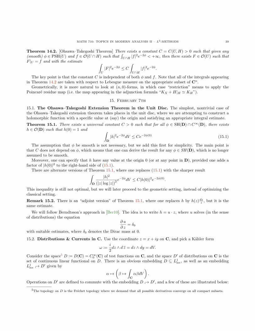
1.1. Example 1: The Ohsawa–Takegoshi Theorem. This is an extension theorem, that comes in twoversions: a function-theoretic version and a geometric one.
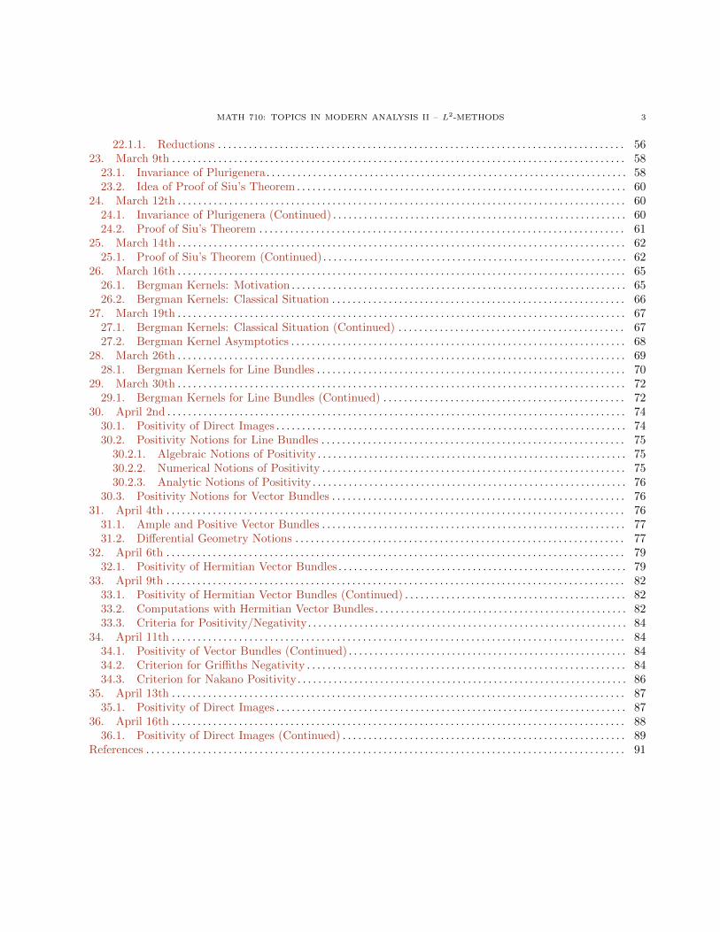
(A) Function-theoretic version. In this form, the result is due to Ohsawa–Takegoshi [OT87]. Let D ⊆ Cdenote the open unit disc. Assume Ω ⊆ Cn−1 ×D is a pseudoconvex domain, and set Ω′ = Ω ∩ zn = 0. Thebasic picture is the following:
zn = 0
Ω′
Ω
Figure 1. The (vertical) hyperplane zn = 0 intersects the ball Ω in the domain Ω′.
Then, for every plurisubharmonic function ϕ ∈ PSH(Ω) and every holomorphic function f ∈ O(Ω′) such that∫Ω′|f |2e−2ϕdλ < +∞,
there exists F ∈ O(Ω) such that F |Ω′ = f , and∫Ω
|F |2e−2ϕdλ ≤ π∫
Ω′|f |2e−2ϕdλ
where dλ denotes the Lebesgue measure (on Ω or on Ω′, as appropriate). The above integral inequality is calleda ‘weighted L2-estimate’.
When one proves this theorem, one generally replaces the term π by a positive constant depending only onthe domain Ω. With additional work, one can show (in the above setup) that the optimal such constant is π;see [Bo13].
(B) Geometric version. In this form, the result is due to Manivel [Man93] and Siu [Siu96]. Here, we have afibration as pictured below:More precisely, let π : X → D be a proper holomorphic submersion (so each fibre of π is a compact complexmanifold). Let L be a holomorphic line bundle on X, and φ a semipositive (singular) metric on L. WriteL0 := L|X0
. Then, given a section s0 ∈ H0(X0,KX0+ L0) (i.e. s0 is an L0-valued holomorphic n-form on X0,
where n is the dimension of any fibre of π), there exists s ∈ H0(X,KX + L) such that “s|X0= s0” (in the sense
of adjunction) and ∫X
|s|2e−2φ ≤ C∫X0
|s0|2e−2φ|L0
for some constant C > 0 independent of φ and f .In the formalism that will be set up later in the class, the expression |s|2e−2φ is a volume form on X, so we
do not need to include the Lebesgue measure in the above integrals.
MATH 710: TOPICS IN MODERN ANALYSIS II – L2-METHODS 5
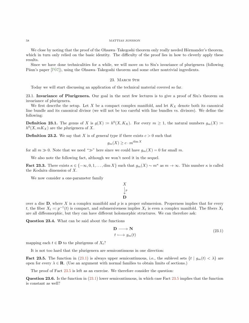
X
D0
X0
t
Xt
π
Figure 2. The fibre of π above a point t ∈ D is denoted by Xt.
The geometric version of the Ohsawa–Takegoshi theorem fits into a more general theme in complex geometry,where one takes an object on the central element of some family and extends it to the whole family in a controlledway. These techniques are very useful.
The method for solving this is a collection of techniques in several complex variables known as the Hormander-Skoda theorems, namely solving the ∂-equation, which we will discuss next.
1.2. Example 2: The Hormander(-Skoda) Theorem. The idea is to solve the equation ∂ u = f withestimates, where f is a given holomorphic (p, q)-form.
(A) Function-theoretic version. Let Ω ⊆ Cn be a pseudoconvex (ψcx) domain (e.g. the unit ball) andϕ ∈ PSH(Ω)∩C∞(Ω). In addition, we require that ϕ is strictly plurisubharmonic: there exists a constant c > 0such that
n∑j,k=1
∂2 ϕ
∂ zj ∂ zk(z)wjwk ≥ c
n∑j=1
|wj |2
for z ∈ Ω and w ∈ Cn, where the terms of the left-hand side form the complex Hessian of ϕ at z. If q > 0, thenfor any smooth (p, q)-form f on Ω with ∂ f = 0, there exists a smooth (p, q)-form u on Ω such that ∂ u = f and∫
Ω
|u|2e−2ϕdλ ≤ 1
c
∫Ω
|f |2e−2ϕdλ
provided the right-hand side is finite.This is one of many different versions of this theorem, but it is the one with which we will begin. In principle,
this is a PDE that we will solve using Hilbert space methods.(B) Geometric version. Let (X,ω) be a Kahler manifold of dimension n (i.e. X is a complex manifold and
ω is a closed, positive (1, 1)-form on X). Let L be a holomorphic line bundle on X, and φ a (smooth) positivemetric on L. Suppose that
ddcφ ≥ cωas (1, 1)-forms, for some positive constant c > 0 (the form ddcφ is some kind of curvature of the metric φ). Ifq > 0, then given any ∂-closed (n, q)-form f with values in L such that ∂ f = 0, there exists an (n, q − 1)-formu with values in L such that ∂ u = f and∫
X
|u|2e−2φ ≤ 1
cq
∫X
|f |2e−2φ,
provided the right-hand side is finite.As before, the formalism is set up in such a way that |u|2e−2φ is a volume form on X.
Remark 1.1. If X is projective (and L is ample), then this can be viewed as a “quantitative” version of theKodaira vanishing theorem, which says that Hq(X,KX + L) = 0 for q > 0. Similarly, a suitable version of theOhsawa–Takegoshi theorem can be viewed as a version of inversion of adjunction.
6 MATTIAS JONSSON
1.3. Other Topics. Once we have discussed Examples 1 and 2, we can move on to further topics, some of whichare listed below.
• Berndtsson’s theorem on the positivity of direct images1 [Ber09];
• Siu’s theorem on the invariance of plurigenera [Siu98, P07];• Nadel’s vanishing theorem [Nad90];• Singularities of plurisubharmonic functions.
The exact material to be covered will depend on time and the interests of the audience.
1.4. Review of Several Complex Variables. Let Ω ⊆ Cn be an open subset.
Definition 1.2. A holomorphic function on Ω is a function f : Ω → C that is complex differentiable: that is,for any z ∈ Ω, there exists a complex-linear map f ′(z) : Cn → C such that
f(z + w) = f(z) + f ′(z)w + o(w)
for w ∈ Cn as w → 0.
As in complex analysis, there is alternate definition in terms of power series.
Definition 1.3. A function f : Ω → C is analytic if for any z ∈ Ω, there exists ε > 0, cα ∈ C (α ∈ Nn) suchthat
∑α |cα|ε|α| < +∞ and
f(z + w) =∑α
cαwα
when w ∈ Cn satisfies |wj | ≤ ε and z + w ∈ Ω.
One of the miracles of several complex variables is that one can show the following, using Cauchy’s formulafor polydiscs.
Theorem 1.4. Holomorphic and analytic functions coincide.
As an aside, if one naively attempts to use these definitions over a non-Archimedean field (e.g. Qp), thenthese two definitions need not coincide.
2. January 5th
While later in the course we will move on to more geometric aspects, we must first work in Cn for the nextfew lectures. For this material, we are following Hormander’s book [H90], and there are also nice notes by BoBerndtsson [Ber10].
2.1. The ∂-Equation in Cn. Fix coordinates (z1, . . . , zn) on Cn. For 0 ≤ p, q ≤ n, a (p, q)-form is a differentialform of the form
f =∑
|I|=p,|J|=q
fI,JdzI ∧ d zJ
where I = (i1, . . . , ip) and J = (j1, . . . , jq) are multi-indices, the fI,J ’s are functions, and
dzI ∧ d zJ := dzi1 ∧ . . . ∧ dzip ∧ d zj1 ∧ . . . d zjq .
We may assume there are no repetitions in the multi-indices I or J , as otherwise the differential form dzI ∧ d zJis zero.
The usual exterior derivative operator d on differential forms can be decomposed as d = ∂+ ∂, where ∂ and∂ are defined as follows: if f is a (p, q)-form, then ∂ f is the (p+ 1, q)-form given by
∂ f :=∑I,J
∂ fI,JdzI ∧ d zJ
1The function-theoretic version of this result is known as the ‘subharmonic variation of Bergman kernels’ in the literature.
MATH 710: TOPICS IN MODERN ANALYSIS II – L2-METHODS 7
and ∂ f is the (p, q + 1)-form given by
∂ f :=∑I,J
∂ fI,JdzI ∧ d zJ ,
where
∂ fI,J :=
n∑k=1
∂ fI,J∂ zk
dzk and ∂ fI.J :=
n∑k=1
∂ fI,J∂ zk
d zk .
The relation d2 = 0 implies that ∂2 = ∂ ∂+ ∂ ∂ = ∂2
= 0.Given an open set U ⊆ Cn, set
C∞(p,q)(U) := (p, q)-forms on U with C∞-coefficients .
These give rise to the Dolbeault cohomology group Hp,q(U) on U , which is given by
Hp,q(U) :=ker(∂ : C∞(p,q)(U)→ C∞(p,q+1)(U)
)im(∂ : C∞(p,q−1)(U)→ C∞(p,q)(U)
) .In the above definition, we are implicitly assuming that q ≥ 1. implicitly assuming here that q ≥ 1. One canshow the following comparison theorem:
Theorem 2.1. [Dolbeault’s Theorem] There is an isomorphism
Hp,q(U) ' Hq(U,ΩpU ),
where the right-hand side is sheaf cohomology on U with values in the sheaf ΩpU of holomorphic p-forms on U .
The main ingredient in the proof of Dolbeault’s theorem (modulo standard sheaf-theoretic yoga) is the fol-lowing lemma.
Lemma 2.2. [∂-Poincare Lemma] If U ⊆ Cn is a polydisc or a ball, then Hp,q(U) = 0 for 0 ≤ p ≤ n and1 ≤ q ≤ n.
This is a complex analogue of the usual Poincare lemma for the d-operator in Rn. One of the first goals ofthe class is to show the following generalization.
Goal 2.3. If U ⊆ Cn is a pseudoconvex domain, prove that Hp,q(U) = 0 using Hilbert space methods.
One should think of pseudoconvex domains as a kind of generalized convex domains with no interestingtopology, and we will discuss them in more depth later.
Let U ⊆ Cn be an open set. Set
L2(U, loc) :=
f : U → C (Lebesgue) measurable function such that
∫K
|f |2dλ < +∞ for all K b U
.
Strictly speaking, we should mod out by those functions that are equal outside a set of measure zero, but wewill ignore this issue. Fix a “weight” ϕ ∈ C0(U), and set
L2(U,ϕ) :=
f ∈ L2(U, loc) :
∫U
|f |2e−2ϕdλ < +∞
This is a Hilbert space with the inner product defined by
〈f, g〉 :=
∫U
fge−2ϕdλ
8 MATTIAS JONSSON
for f, g ∈ L2(U,ϕ). There are versions of these spaces for forms: let L2(p,q)(U, loc) denote the space of (p, q)-forms
with coefficients in L2(U, loc), and let L2(p,q)(U,ϕ) denote the space of (p, q)-forms with coefficients in L2(U,ϕ).
These are both Hilbert spaces with norms defined as follows: if f =∑I,J fI,Jdz
I ∧ d zJ , define the function
|f |2 :=∑I,J
|fI,J |2 : U → [0,+∞]
and declare
‖f‖2 :=
∫U
|f |2e−2ϕdλ
Both L2(U, loc) and L2(U,ϕ) are Hilbert spaces with respect to the above norm.Furthermore, adopting the notation from the theory of distributions, set
D(U) := C∞0 (U) := C∞-functions on U with compact support .
The functions in D(U) are often called the test functions on U . Similarly, set
D(p,q)(U) := (p, q)-forms on U with coefficients in D(U) ,
and elements of this space are known as test (p, q)-forms.
Lemma 2.4. For any weight ϕ ∈ C0(U), D(p,q)(U) is dense in L2(p,q)(U,ϕ).
Sketch. The idea is to use convolution to approximate an arbitrary function a smooth, compactly-supportedone. By approximating the coefficients of a form, we may assume that p = q = 0. Given f ∈ L2(U,ϕ), we mayassume that there is a compact set K b U such that supp(f) ⊆ K (indeed, replace f by f · 1K for a sufficientlylarge compact set K b U). Now, pick a test function χ ∈ D(Cn) such that
∫Cn
χdλ = 1 (and one can alsoassume that χ ≥ 0, and χ ≡ 1 in a neighbourhood of 0). For ε > 0, set
χε(z) := ε−2nχ(z/ε).
That is, we have shrunk the support of χ but maintained that the integral be 1. For 0 < ε 1, one can checkthat f ∗ χε ∈ D(U) and f ∗ χε → f in L2(U,ϕ) as ε→ 0.
Now, fix 3 weights2 ϕ1, ϕ2, ϕ3 ∈ C0(U). Given (p, q) with 0 ≤ p ≤ n and 1 ≤ q ≤ n, consider the following 3Hilbert spaces:
H1 := L2(p,q−1)(U,ϕ1)
H2 := L2(p,q)(U,ϕ2)
H3 := L2(p,q+1)(U,ϕ3)
and there is a diagram
H1T :=∂−→ H2
S:=∂−→ H3
of maps between these Hilbert spaces, where one formally has S T = 0.
Problem 2.5. The maps T and S are not everywhere defined! They are (as we will see) closed, densely-defined,unbounded linear maps.
2This is why Hormander’s method is often referred to as the “method of 3 weights”.
MATH 710: TOPICS IN MODERN ANALYSIS II – L2-METHODS 9
2.2. Hilbert Space Digression. Let H1 and H2 be (complex) Hilbert spaces. A (possibly) unbounded linearmap from H1 to H2 is a pair (DT , T ), where DT ⊆ H1 is a linear subspace and T : DT → H2 is a linear map.Usually, we simply write T for the pair (DT , T ).
We say T is densely-defined if DT ⊆ H1 is dense, and say T is closed if the graph
ΓT := (u, Tu) : u ∈ DT ⊆ H1 ×H2
is closed. More concretely, if un ∈ DT and un → u ∈ H1 and Tun → f ∈ H2, then u ∈ DT and Tu = f .For many purposes, closed and densely-defined linear maps behave similarly to bounded linear maps.
Theorem 2.6. [Definition of Adjoints] If T : H1 → H2 is closed and densely-defined, then there exists a uniqueclosed and densely-defined linear map T ∗ : H2 → H1 such that
〈u, T ∗f〉H1= 〈Tu, f〉H2
(2.1)
for any u ∈ DT and f ∈ DT∗ .
Proof. We begin by defining the domain of the adjoint operator to be
DT∗ := f ∈ H2 : ∃ C > 0 such that |(Tu, f)| ≤ C‖u‖1 for all u ∈ DT .
For f ∈ DT∗ , the map u 7→ (Tu, f) is a bounded linear functional on DT . As DT is dense, this extends to allof H1. By the Riesz representation theorem, there is a unique v ∈ H1 such that (Tu, f) = (u, v) for u ∈ DT .Set T ∗f := v. One must now check that T ∗ is closed and densily-defined. The idea is to work on the graphΓT ⊆ H1 ×H2 and use the closedness of T , which we will explain next time.
3. January 8th
Today, we will continue to discuss the functional analysis necessary to solve the ∂-equation in Cn, i.e. to solve∂ u = f provided ∂ f = 0.
3.1. The ∂-Equation on Domains in Cn. If U ⊆ Cn is an open subset, and a weight ϕ ∈ C0(U), considerthe Hilbert space
L2(p,q)(U,ϕ) :=
(p, q)-forms f with L2(U, loc)-coefficients such that
∫U
|f |2e−2ϕ < +∞,
inside of which lies the dense subset D(p,q)(U) of test forms. Given two weights ϕ1, ϕ2 ∈ C0(U), consider themap
T := ∂ : L2(p,q−1)(U,ϕ1)→ L2
(p,q)(U,ϕ2).
Last time, we asserted the following:
Lemma 3.1. The map T is closed and densely-defined.
Proof. The domain of T is
DT =f ∈ L2
(p,q−1)(U,ϕ1) : ∂ f ∈ L2(p,q)(U,ϕ2)
,
where ∂ f is computed as a current (i.e. a form whose coefficients are distributions). It is clear that DT containsD(p,q−1)(U), so we have that T is densely-defined.
It remains to show that the map T is closed, i.e. the graph ΓT is closed. Suppose that (un, Tun) ∈ ΓTand (un, Tun) → (u, f) ∈ L2
(p,q−1)(U,ϕ1)× L2(p,q)(U,ϕ2). Then, un → u and ∂ un → f in the sense of currents.
Differentiation is (almost by definition) made to be continuous on the space of currents, so it follows that ∂ u = f .Thus, u ∈ DT and Tu = f .
10 MATTIAS JONSSON
3.2. Functional Analysis Background. It is not enough to deal with bounded maps between Hilbert spaces(because differentiation tends not to be a bounded operation), so we instead work with closed and densely-definedoperators.
Theorem 3.2. [Definition of Adjoints] If T : H1 → H2 is a closed and densely-defined map between Hilbertspaces, then there exists a unique closed and densely-defined linear map T ∗ : H2 → H1 such that
〈Tu, f〉H2= 〈u, T ∗f〉H1
for u ∈ DT and f ∈ DT∗ . Furthermore,
(1) ker(T ∗) = im(T )⊥ and ker(T ) = im(T ∗)⊥;
(2) im(T ) = ker(T ∗)⊥ and im(T ∗) = ker(T )⊥;(3) T ∗∗ = T .
More generally, to any closed and densely-defined linear map X → Y between Banach spaces, there is anadjoint Y ∗ → X∗ between the corresponding dual spaces.
Proof. The domain of T ∗ is
DT∗ := f ∈ H2 : ∃C > 0 such that |〈Tu, f〉H2| ≤ C‖u‖1 for all u ∈ DT .
The density of DT in H1 (along with the Riesz representation theorem) implies that for all f ∈ DT∗ , there existsv ∈ H1 such that 〈Tu, f〉H2 = 〈u, v〉H1 for all u ∈ DT . Set T ∗f := v.
It is clear that T ∗ : DT∗ → H1 is linear, and we must show that T ∗ is closed and densely-defined. Define theisometry J : H1 ×H2 → H2 ×H1 by
(u, f) 7→ (−f, u).
Then, one can check that ΓT∗ = J(ΓT )⊥, which implies that T ∗ is closed. (In fact, since the orthogonalcomplement of a subspace is always closed, this argument shows that T ∗ is closed even without assuming thatT is closed.)
To prove that DT∗ is dense in H2, pick g ∈ D⊥T∗ and we must show that g = 0. Observe that
(g, 0) ∈ Γ⊥T∗ = J(ΓT ) = (−Tu, u) : u ∈ DT .
This implies that g = 0. It is now easy to prove (1-3) using the fact that ΓT∗ = J(ΓT ) (and this is left as anexercise).
Consider the following real-variable example.
Example 3.3. Consider H1 = H2 = H = L2(R, x2/4) and T = ddx : H1 → H2, with DT = u ∈ H : u′ ∈ H,
where u′ is computed in the sense of distributions. We want to compute both DT∗ and T ∗.The formal adjoint is defined using only test functions, i.e. we demand 〈Tu, f〉 = 〈u, T ∗f〉 for u, f ∈ D(R).
This can be rewritten as ∫ ∞−∞
u′ · f · e−x2/2dx =
∫ ∞−∞
u · T ∗f · e−x2/2dx,
and, using integration by parts, the first integral is given by
−∫ ∞−∞
ud
dx
(f · e−x
2/2)dx
where the boundary term vanishes by construction. Thus, the formal adjoint is
T ∗formal(f) := −f ′ + xf,
where the right-hand side is computed in the sense of distributions. We claim that
DT∗ = f ∈ H : − f ′ + xf ∈ H
MATH 710: TOPICS IN MODERN ANALYSIS II – L2-METHODS 11
and T ∗f = −f ′ + xf for f ∈ DT∗ . The proof of the claim is an approximation argument: pick χ ∈ D(R) suchthat χ ≥ 0, χ ≡ 1 near 0, and set χk(x) := χ(x/k) for k ∈ N. If u ∈ DT and −f ′ + xf ∈ H, then
〈u,−f ′ + xf〉 = limk→+∞
⟨χku︸︷︷︸∈DT
,−f ′ + xf
⟩= limk→+∞
〈(χku)′, f〉 = limk→+∞
⟨χ′k︸︷︷︸→0
·u+ χk · u′, f
⟩= 〈u′, f〉,
which completes the proof of the claim.
Remark 3.4. If we replace R by (0, 1) in Example 3.3 (and keep all else the same), then the formal adjointremains the same; however, the domain DT∗ is smaller than expected. For example, suppose f ∈ C∞([0, 1]);when is f ∈ DT∗? One requires that there exists C > 0 such that
C · ‖u‖ ≥ |〈Tu, f〉| =∣∣∣∣∫ 1
0
u′ · f · e−x2/2dx
∣∣∣∣ = u(1)f(1)e−1/2 − u(0)f(0)︸ ︷︷ ︸=(∗)
−∫ 1
0
u · (fe−x2/2)′dx
for (at least) all u ∈ C∞([0, 1]). In order for this estimate to hold, the terms (∗) must vanish. Thus, a necessarycondition for f ∈ DT∗ ∩ C∞([0, 1]) is that f(0) = f(1) = 0.
The lesson to take away from Example 3.3 and Remark 3.4 is that boundary phenomena are very annoyingto deal with when using these Hilbert space methods, but we will avoid them by picking weights that render theboundary irrelevant.
We will use functional analysis to prove existence of solutions using a priori estimates, such as the oneappearing the lemma below.
Lemma 3.5. Let T : H1 → H2 be a closed and densely-defined linear map between Hilbert spaces. Then, thefollowing are equivalent:
(1) im(T ) is closed;
(2) there exists δ > 0 such that ‖T ∗f‖ ≥ δ‖f‖ for all f ∈ im(T ) ∩DT∗ .
We will later apply this lemma to the sequence of maps H1∂−→ H2
∂−→ H3 and for f ∈ H2 such that ∂ f = 0.
We then want to solve the equation ∂ u = f , and we will somehow know that f ∈ im(∂). Then, we will provean estimate as in Lemma 3.5.
4. January 10th
There are some notes [Jon18] on the course website that contain more of the details of the functional analysisbackground that we have been discussing.
4.1. Functional Analysis Background (Continued).
Lemma 4.1. Let T : H1 → H2 be a closed and densely-defined linear map. Then, the following are equivalent:
(a) im(T ) is closed;
(b) there exists δ > 0 such that ‖T ∗f‖H1≥ δ‖f‖H2
for all f ∈ im(T ) ∩DT∗ .
In this case, given f ∈ im(T ) = im(T ), there exists u ∈ DT such that Tu = f and ‖u‖ ≤ δ−1‖f‖.
Proof. For (b ⇒ a), pick g ∈ im(T ), then one has the estimate
|〈g, f〉H2 | ≤ δ−1‖g‖H2‖T ∗f‖H1 , f ∈ DT∗ (4.1)
Indeed, decompose H2 = im(T )⊕im(T )⊥
, and (4.1) follows from (b) for f ∈ DT∗∩im(T ), and (4.1) is obvious for
f ∈ DT∗ ∩ im(T )⊥
. Now, (4.1) implies that the antilinear form T ∗f 7→ 〈g, f〉H2, defined on im(T ∗), is bounded.
By Hahn–Banach and the Riesz representation theorem, there exists u ∈ H1 such that
〈g, f〉H2= 〈u, T ∗f〉H1
, f ∈ DT∗
12 MATTIAS JONSSON
This says that g = T ∗∗u = Tu. Furthermore, ‖u‖H1≤ δ−1‖g‖H2
.Conversely, for (a ⇒ b), we must prove that the set
B :=f ∈ im(T ) ∩DT∗ : ‖T ∗f‖H1
≤ 1⊆ im(T ) ⊆ H2
is bounded. The uniform boundedness principle implies that it suffices to show that
supf∈B|〈f, g〉H2 | < +∞
for all g ∈ im(T ). However, the assumption (a) implies that g = Tu for some u ∈ DT , so
|〈f, g〉H2| = |〈f, Tu〉H2
| = |〈T ∗f, u〉H1| ≤ ‖u‖H1
< +∞,where the final inequality follows from Cauchy–Schwarz.
We will record, without proof, some further results that we will use; see [Jon18] for the proofs.
Lemma 4.2. If T : H1 → H2 is closed, then the following are equivalent:
(a) im(T ) is closed;(b) there exists δ > 0 such that ‖Tu‖H2
≥ δ‖u‖H1for all u ∈ ker(T )⊥ ∩DT .
If T were everywhere-defined and bounded, then it is easy to sketch out the idea of Lemma 4.2: replace H2
by im(T ) to assume that the image is dense, and replace H1 by the ker(T )⊥ to assume that T is injective. Then,assuming (a), the Banach open mapping theorem implies (b); the converse is easy. When T is not necessarilyeverywhere, one can employ a similar strategy, but one must instead work on the graph of T .
The upshot of Lemma 4.1 and Lemma 4.2 is that, when T is both closed and densely-defined, then there areestimates on both T and T ∗.
An immediate corollary of Lemma 4.2 is the following result (which also holds for Banach spaces).
Corollary 4.3. [Banach Closed Range Theorem] If T is a closed and densely-defined map between Hilbert spaces,then im(T ) is closed iff im(T ∗) is closed.
Now, consider the situation where we have closed and densely-defined maps
H1T→ H2
S→ H3
between Hilbert spaces and assume that this is a complex, in the sense that im(T ) ⊆ ker(S) In this case, writeS T = 0. It is easy to check that we also have T ∗ S∗ = 0.
Lemma 4.4. In the setting above, there is an orthogonal decomposition
H2 = (ker(S) ∩ ker(T ∗))⊕ im(T )⊕ im(S∗),
and the following are equivalent:
(a) im(T ) = ker(S) and im(S∗) = ker(T ∗);(b) there exists δ > 0 such that ‖Sf‖2H1
+ ‖T ∗f‖H3 ≥ δ2‖f‖2H2for all f ∈ DS ∩DT∗ .
Lemma 4.4 follows formally from the previous results.
4.2. The ∂-Equation in Dimension 1. The plan is to first discuss the solution of the ∂-equation in thedimension 1 case (i.e. for domains in C) following [Ber10], and then to proceed to the geometric version (i.e.extension of sections of line bundles on manifolds).
Let U ⊆ C be an open subset (we will see later that U is pseudoconvex). Let φ ∈ C2(U) ∩ SH(U) be a“smooth”, subharmonic function on U . In fact, we assume that φ is strictly subharmonic, in the sense that
∆φ := 2∂2 φ
∂ z ∂ z> 0.
MATH 710: TOPICS IN MODERN ANALYSIS II – L2-METHODS 13
A solution of the ∂-equation with estimates, which is slightly different from the one discussed previously, is thefollowing theorem.
Theorem 4.5. If f ∈ L2(0,1)(U, loc), then there exists u ∈ L2(U, loc) such that ∂ u = f and∫
U
|u|2e−2φdλ ≤∫U
|f |2
∆φe−2φdλ,
provided the right-hand side is finite.
Theorem 4.5 admits the following (arguably slightly cleaner) corollary.
Corollary 4.6. If ∆φ ≥ δ > 0, then for any f ∈ L2(0,1)(U, φ), there exists u ∈ L2(U, φ) such that ∂ u = f and∫
U
|u|2e−2φdλ ≤ 1
δ
∫U
|f |2e−2φdλ,
provided the right-hand side is finite.
We will aim to prove Corollary 4.6, bypassing the proof of Theorem 4.5. One can make sense of Corollary 4.6without the smoothness assumption on φ, where ∆φ is now well-defined only as a positive measure on U , asopposed to a function (but we will ignore this complication for now).
We follow the Hilbert space approach:
H1 = L2(U, φ)T=∂−→ H2 = L2
(0,1)(U, φ)S=0−→ H3 = 0.
By general results, it suffices to prove the estimate
‖T ∗f‖ ≥ δ‖f‖ (4.2)
for all f ∈ DT∗ . The proof of (4.2) is broken down into two steps:
(1) prove the estimate when f ∈ D(0,1)(U) is a test form;(2) deduce the estimate in general via a suitable approximation technique.
To show (1), take a test form f ∈ D(0,1)(U) and write f = fdz for some test function f ∈ D(U). In this case,
the Hilbert space adjoint agrees with the formal adjoint ∂∗φ on test forms. One can compute ∂
∗φ by integration
by parts, i.e. for all u ∈ D(U) and f ∈ D(0,1)(U)∫U
u∂∗φ fe
−2φ =
∫U
∂ u · fe−2φ.
This implies that
∂∗φ f = −e2φ ∂
(e−2φf
)= −∂ f
∂ z+ 2
∂ φ
∂ zf .
Proposition 4.7. [Basic Identity] If f = fdz ∈ D(0,1)(U), then∫U
∆φ · |f |2e−2φdλ+
∫U
∣∣∣∣∣∂ f∂ z∣∣∣∣∣2
e−2φdλ =
∫U
| ∂∗φ f |2e−2φdλ.
Granted Proposition 4.7, if one assumes that ∆φ ≥ δ > 0, then one obtains the estimate∫U
| ∂∗φ f |2e−2φdλ ≥ δ∫U
|f |2e−2φdλ,
which completes Step 1.
Remark 4.8. The proof of Proposition 4.7 is easy, but it has interesting generalizations in (higher-dimensional)geometric situations. These are often called Bochner-type identities.
14 MATTIAS JONSSON
5. January 12th
The goal for today is to finish the solution of the ∂-equation in dimension 1, following Berndtsson’s notes [Ber10]as well as Hormander’s original paper [H65].
5.1. The ∂-Equation in Dimension 1 (Continued). Let U ⊆ C be an open subset, let φ ∈ C2(U) be strictlysubharmonic (more precisely, there exists a constant c > 0 such that ∆φ ≥ c on U).
Theorem 5.1. For any f ∈ L2(0,1)(U, φ), there exists u ∈ L2(U, φ) such that ∂ u = f and∫
U
|u|2e−2φdλ ≤ 1
c
∫U
|f |2e−2φdλ,
provided the right-hand side is finite.
If z is the coordinate on C, then write f = fdz (so |f | := |f |). By the functional-analytic results from lasttime, it suffices to prove an estimate of the form
‖T ∗f‖2 ≥ c‖f‖2, (5.1)
for all f ∈ DT∗ , where T ∗ is the Hilbert space adjoint of the operator T := ∂, which we view as a closed anddensely-defined map T : L2(U, φ)→ L2
(0,1)(U, φ).
There is also the formal adjoint ∂∗φ : D(0,1)(U)→ D(U) defined by
〈∂ u, f〉 = 〈u, ∂∗φ f〉
for u ∈ D(U) and f ∈ D(0,1)(U). By (e.g.) Stokes’ theorem, one finds that
∂∗φ f = −∂ f
∂ z+ 2
∂ φ
∂ zf . (5.2)
for f ∈ D(0,1)(U).
Remark 5.2.
(1) It is clear that D(0,1)(U) ⊆ DT∗ and T ∗ = ∂∗φ on D(0,1)(U).
(2) If, say, U is bounded and has C1-boundary, then one can define ∂∗φ f for f ∈ C1
(0,1)(U) (i.e. f is the
restriction to U of some (0, 1)-form defined on C with C1-coefficients), but it is not clear that f ∈ DT∗
because of boundary contributions in Stokes’ formula.
Proposition 5.3. [Basic Identity] If f = fdz ∈ D(0,1)(U) is a test form, then∫U
∆φ · |f |2e−2φdλ+
∫U
∣∣∣∣∣∂ f∂ z∣∣∣∣∣2
e−2φdλ =
∫U
∣∣∣∂∗φ f ∣∣∣2 e−2φdλ.
An immediate corollary of the basic identity, obtained by throwing away the second term on the left-handside, is the following:
Corollary 5.4. If ∆φ ≥ c > 0, then ‖T ∗f‖2 ≥ c‖f‖2 for all f ∈ D(0,1)(U).
Lemma 5.5. If f = fdz ∈ D(0,1)(U), then
∂
∂ z
(∂∗φ f)− ∂∗φ
(∂ f)
= f∆φ.
The proof of Lemma 5.5 is an easy exercise, granted the formula (5.2).
MATH 710: TOPICS IN MODERN ANALYSIS II – L2-METHODS 15
Proof of the Basic Identity. Observe that∫U
| ∂∗φ f |2e−2φdλ =
∫U
∂∗φ f · ∂
∗φ f2−2φdλ
=
∫U
∂
∂ z
(∂∗φ f)f e−2φdλ
Lemma 5.5=
∫U
∂∗φ
(∂ f
∂ z
)f e−2φdλ+
∫U
f∆φfe−2φdλ
=
∫U
∣∣∣∣∣∂ f∂ z∣∣∣∣∣2
e−2φdλ+
∫U
∆φ · |f |2e−2φdλ.
In order to apply the functional analytic results, we require the estimate ‖T ∗f‖2 ≥ c‖f‖2 for all f ∈ DT∗ ,but we only have it so far for f ∈ D(0,1)(U). It is enough to show that D(0,1)(U) ⊆ DT∗ is dense for the graphnorm
f 7→(‖f‖2 + ‖T ∗f‖2
)1/2.
Unfortunately, it is not clear whether or not this is true (in fact, Mattias suspects it is false).Following Hormander’s paper, we first assume that U has C2-boundary. Let Ck(U) denote the image of
the restriction map Ck(C) → C0(U), and let Ck(U) ⊆ Ck(U) denote the functions vanishing outside of somecompact set (equivalently, some disc). Similarly, one can define Ck(0,1)(U) and Ck(0,1)(U) and so on.
(a) The set C1(0,1)(U) is dense in DT∗ for the graph norm.
(b) The set C1(U) is dense in DT for the graph norm.
We will not prove the approximation lemma now, but will see (and prove) other versions later.The question is now: how to use the fact that U has C2-boundary? One can pick ρ ∈ C2(U) such that
• ρ < 0 on U ;• ρ = 0 on ∂ U ;• |∇ρ| = 1 on ∂ U .
The last condition can be achieved using partitions of unity. One can use this function to control boundaryintegrals in Green’s (or Stokes’) formula. These calculations lead to the following:
Lemma 5.7. If f = fdz ∈ C1(0,1)(U), then f ∈ DT∗ iff f |∂ U ≡ 0.
Corollary 5.8. The basic identity holds for f ∈ C1(0,1)(U) ∩DT∗ .
The proof of Corollary 5.8 is identical to the proof of Proposition 5.3, because the boundary integrals vanishby Lemma 5.7.
Corollary 5.9. There exists c > 0 such that ‖T ∗f‖2 ≥ c‖f‖2 for all f ∈ DT∗ .
Proof. The estimate is ok by basic identity for f ∈ C1(0,1)(U) ∩DT∗ , and it is true in general by density.
Therefore, we have shown Hormander’s theorem (Theorem 5.1) is true when U has C2-boundary. Now,consider a general open set U ⊆ C, and the idea is to exhaust U from the inside by smooth, bounded domains:write U =
⋃∞j=1 Uj , where Uj b U has C2-boundary (and Uj ⊆ Uj+1). For all j ≥ 1, there exists uj ∈ L2(Uj , φ)
such that ∂ uj = f |Uj and ∫Uj
|uj |2e−2φdλ ≤ 1
c
∫Uj
|f |2e−2φdλ ≤ 1
c
∫U
|f |2e−2φdλ.
16 MATTIAS JONSSON
Extend uj to all of U , and take the weak limit u of the uj ’s in L2(U, φ), i.e. (after possibly passing to asubsequence) uj → u weakly in L2(U, φ), and hence uj → u in the sense of distributions. Thus, (on any compact
subset) ∂ u = limj ∂ uj = limj fj = f on U , and
‖u‖ ≤ lim infj→+∞
‖uj‖ ≤1
c‖f‖2.
One must be careful to make this all precise.Next time, we will begin aiming towards a version of Hormanders theorem for metrics on line bundles on
Kahler manifolds.
6. January 17th
Today, we will discuss Hormander’s theorem for (0, 1)-forms in Cn, the best reference for which are Berndts-son’s notes [Ber95]. Most calculations will be skipped, and we will focus instead on the ingredients of theproof.
6.1. The ∂-Equation in Higher Dimensions. The goal is to solve the equation
∂ u = f,
where f ∈ L2(0,1)(U, loc) satisfies ∂ f = 0 and u ∈ L2(U, loc). Write f =
∑nj=1 fjdzj . Consider a pseudoconvex
open set U ⊆ Cn with C2-boundary; that is.
• we can write U = ρ < 0 for some ρ ∈ C2(Cn), where ∇ρ 6= 0 on ∂ U = ρ = 0;• if p ∈ ∂ U and a ∈ Cn lies in the tangent space at p (i.e.
∑nj=1
∂ ρ∂ zj
(p)aj = 0), then
n∑j,k=1
ρjkajak ≥ 0, (6.1)
where ρjk = ∂2 ρ∂ zj ∂ zk
(p) are the components of the complex Hessian. (Note that this is slightly weaker
than saying ρ is plurisubharmonic, which would require (6.1) to hold for all a ∈ Cn.)
Now, consider a weight φ ∈ C2(U) and assume φ is strictly psh, i.e. the matrix (φjk)nj,k=1 is a positive Hermitian
(and we write (φjk)nj,k=1 > 0). Set (φjk) := (φjk)−1 to be the inverse matrix.
Theorem 6.1. Suppose f ∈ L2(0,1)(U, loc) satisfies ∂ f = 0. Then, there exists u ∈ L2(U, loc) such that ∂ u = f
and ∫U
|u|2e−2φ ≤ 1
2
∫U
n∑j,k=1
φjkfjfke−2φ
provided the right-hand side is finite.
In one variable, this right-hand side is simply |f |2 divided by the Laplacian of φ, as in Theorem 4.5. Unlessotherwise specified, all integrals are taken with respect to Lebesgue measure, so this added notation is oftenomitted.
The setup from before was to consider the “exact” sequence
L2(U, φ)T−→ L2
(0,1)(U, φ)S−→ L2
(0,2)(U, φ),
where both S and T are the operator ∂, viewed as closed and densely-defined operators.
Lemma 6.2. If α ∈ C1(0,1)(U) ∩DT∗ , then
∑nj=1 αj
∂ ρ∂ zj
= 0 on ∂ U .
Informally, the above lemma says that one can view α as a complex tangent vector to the boundary ∂ U .
Sketch. The proof uses the definition of DT∗ and the divergence theorem.
MATH 710: TOPICS IN MODERN ANALYSIS II – L2-METHODS 17
The Bochner-type identity that is used in this setting is (once again) called the Basic Identity.
Theorem 6.3. [Basic Identity] If α ∈ C2(0,1)(U) ∩DT∗ , then
2
∫U
n∑j,k=1
φjkαjαke−2φ +
∫U
n∑j,k=1
∣∣∣∣∂ αj∂ zk
∣∣∣∣2 e−2φ +
∫∂ U
n∑j,k=1
ρjkαjαke−2φ dS
| ∂ ρ|=
∫U
|∂∗φα|2e−2φ +
∫U
| ∂ α|e−2φ,
where dS is the Lebesgue measure on ∂ U .
The proof of the basic identity is analogous to the previous version. By bounding from below by zero thesecond two terms of the left-hand side of the basic identity, we get the basic inequality.
Corollary 6.4. [Basic Inequality] If α ∈ C2(0,1)(U) ∩DT∗ , then
‖T ∗α‖2 + ‖Sα‖2 =
∫U
| ∂∗φ α|2e−2φ +
∫U
| ∂ α|2e−2φ ≥ 2
∫U
n∑j,k=1
φjkαjαke−2φ.
Observe that the right-hand side of the basic inequality is ≥ δ‖α‖2 for some δ > 0, because of the strictplurisubharmonicity of φ.
One now requires an approximation argument in order to get the basic inequality for all α ∈ DT∗ (in whichcase, one can apply the Hilbert space machinery to conclude).
Theorem 6.5. [Approximation] The subset DS ∩ DT∗ ∩ C∞(0,1)(U) is dense in DS ∩ DT∗ in the graph norm,
which is given by
α 7→(‖α‖2 + ‖Sα‖2 + ‖T ∗α‖2
)1/2.
This is a bit tricky! It is written minimalistically in [H65], and done in more detail in [Ber95].
Corollary 6.6. If α ∈ DS ∩DT∗ , then there exists δ > 0 such that
‖T ∗α‖2 + ‖Sα‖2 ≥ 2
∫U
n∑j,k=1
φjkαjαke−2φ ≥ δ‖α‖2.
Now, Corollary 6.6 and the Hilbert space machinery imply that ker(S) = im(T ), i.e. we can solve the ∂-equation. However, for Theorem 6.1, we need improved estimates.
Proof of Theorem 6.1. Set
C :=
1
2
∫U
n∑j,k=1
φjkfjfke−2φ
1/2
< +∞.
Lemma 6.7. For any α ∈ D(0,1)(U), we have
|〈f, α〉| =∣∣∣∣∫U
f · αe−2φ
∣∣∣∣ ≤ C‖ ∂∗φ α‖.Granted Lemma 6.7, then the rule ∂
∗φ α 7→ 〈f, α〉 defines a bounded, antilinear form L on the set
E :=∂∗φ α : α ∈ D(0,1)(U)
⊆ L2(U, φ).
By Hahn–Banach and the Riesz representation theorem, L can be extended to a bounded linear functional on all
of L2(U, φ) and there exists u ∈ L2(U, φ) such that ‖u‖ ≤ C and L(v) = 〈u, v〉 for all v ∈ L2(U, φ). Set v = ∂∗φ α
for some α ∈ D(0,1)(U), so it follows that∫U
u∂∗φ αe
−2φ = L(∂∗φ α) =
∫U
fαe−2φ.
18 MATTIAS JONSSON
This means that ∂ u = f in the sense of distributions (or really, in the sense of currents). One also has that∫U
|u|2e−2φ = ‖u‖2 ≤ C2 =1
2
∫U
n∑j,k=1
φjkfjfke−2φ,
which completes the proof of Theorem 6.1.
Proof of Lemma 6.7. Use the decomposition L2(0,1)(U, φ) = ker(S) ⊕ ker(S)⊥ to write α = β + γ for some β ∈
ker(S) and γ ∈ ker(S)⊥ ⊆ im(T )⊥ = ker(T ∗) ⊆ DT∗ . As α ∈ D(0,1)(U) ⊆ DT∗ , it follows that β = α− γ ∈ DT∗
and T ∗β = T ∗α. Thus, using that 〈f, γ〉 = 0 since f ∈ ker(S), we have
|〈f, α〉|2 = |〈f, β〉|2
=
∣∣∣∣∫U
f · βe−2φ
∣∣∣∣2≤
2
∫U
n∑j,k=1
φjkβjβke−2φ
1
2
∫U
n∑j,k=1
φjkfjfke−2φ
︸ ︷︷ ︸
=C2
,
where the inequality follows from Cauchy–Schwarz. By Corollary 6.6 (using that Sβ = 0), we get that2
∫U
n∑j,k=1
φjkβjβke−2φ
≤ ‖T ∗β‖2 = ‖T ∗α‖2,
which completes the proof.
Next time, we’ll start moving towards the setting of metrics on line bundles on Kahler manifolds, and theanalogue of Hormander’s theorem in that setting.
7. January 19th
Today, we will begin to discuss some background in complex geometry, the references for which are [Dem12,GH78, Voi02]. The goal, once we have finished with the preliminaries, is to have a version of Hormander’stheorem on compact Kahler manifolds.
7.1. Complex Geometry Background. Let X be a (real) C∞-manifold of dimension 2n. For x ∈ X, wehave TxX ' R2n, where TX is the (real) tangent bundle of X.
Definition 7.1. We say X is a complex manifold if it admits an atlas (Uα, ϕα)α, where Uα ⊆ X is an opensubset and ϕα : Uα → Cn ' R2n is a homeomorphism such that the transition maps ϕα ϕ−1
β are holomorphicfor all α, β.
Definition 7.2. We say X is an almost complex manifold if it admits an almost complex structure, i.e. anendomorphism J : TX → TX of the tangent bundle such that J2 = −id.
It is easy to see that if X is a complex manifold, then X is an almost complex manifold: if (z1, . . . , zn) ∈ Cn
are local coordinates with zj = xj + iyj , then setJ(
∂∂ xj
)= ∂
∂ yj,
J(
∂∂ yj
)= − ∂
∂ xj.
The converse implication is addressed by a deep theorem of Newlander–Nirenberg: an integrable almost complexmanifold is a complex manifold.
MATH 710: TOPICS IN MODERN ANALYSIS II – L2-METHODS 19
We will generally work with the complexified tangent bundle TCX := TX ⊗R C, which is a complex vectorbundle of rank 2n. Locally, TCX is spanned by the vectors
∂
∂ z1, . . . ,
∂
∂ zn,∂
∂ z1, . . . ,
∂
∂ zn,
where
∂
∂ zj=
1
2
(∂
∂ xj− i ∂
∂ yj
)and
∂
∂ zj=
1
2
(∂
∂ xj+ i
∂
∂ yj
).
The endomorphism J extends by C-linearity to J : TCX → TCX, and TCX splits into eigenspaces
TCX = T 1,0X ⊕ T 0,1X,
where T 1,0X = spanj
(∂∂ zj
)has eigenvalue +i, and T 0,1X = spanj
(∂∂ zj
)has eigenvalue −i.
Similarly, there is a decomposition
Λ1CX = Λ1,0X ⊕ Λ0,1X,
where Λ1,0X = span (dz1, . . . , dzn) and Λ0,1X = span (d z1, . . . , d zn). Recall that our conventions aredzj = dxj + idyj ,
d zj = dxj − idyj .
Consequently, we can decompose
ΛrCX =⊕p+q=r
Λp,qX,
where the (p, q)-forms Λp,qX are those of the form∑|I|=p,|J|=q αI,Jdz
I ∧ d zJ . The operator d : ΛrX → Λr+1X
splits as d = ∂+ ∂, where we view ∂ and ∂ as operators ∂ : Λp,qX → Λp+1,q and ∂ : Λp,qX → Λp,q+1X.
Definition 7.3. Write dc := i2π (∂− ∂), and hence ddc := i
π ∂ ∂.
The normalization in the definition of dc is chosen so that the Poincare–Lelong formula looks nice. Forexample, if X = C, then this formula says that
ddc log |z| = δ0
in the sense of currents, where δ0 is the Dirac mass at 0 ∈ C. Said differently, for any test function α ∈ D(C),we have ∫
C
log |z|ddcα = α(0).
Example 7.4. If f : C→ R is a smooth function, then
ddcf =i
4π
(∂
∂ x− i ∂
∂ y
)(∂
∂ x+ i
∂
∂ y
)f(dx+ idy) ∧ (dx− idy)
=1
2π
(∂2 f
∂ x2+∂2 f
∂ y2
)dx ∧ dy.
That is, ddcf agrees (up to scale) with the Laplacian of f , viewed as a measure (equivalently, a top form) on C.
20 MATTIAS JONSSON
7.2. Hermitian Metrics and Forms. Let V be a C-vector space of dimension n (which we will later taketo be holomorphic tangent space at a point). We can also view V as an R-vector space VR of dimension 2n,together with an R-linear endomorphism J : VR → VR such that J2 = −id (that is, J encodes how to multiplyby i). As before, there is a decomposition
VC := VR ⊗R C = V 1,0 ⊕ V 0,1,
where V 1,0 and V 0,1 are the two eigenspaces of J . There is also conjugation on VC, under which V 0,1 = V 1,0.
Lemma 7.5. The following objects are in 1-1 correspondence:
(1) Hermitian forms h : V × V → C (i.e. sesquilinear forms that are conjugate symmetric);(2) symmetric bilinear forms g : VR × VR → R such that g(Jv, Jw) = g(v, w) for all v, w ∈ VR;(3) alternating bilinear forms ω : VR × VR → R of type (1, 1) (i.e. the complexification ω : VC × VC → C
satisfies ω ≡ 0 on V 1,0 × V 1,0 and V 0,1 × V 0,1).
Sketch. The relation between the objects is as follows: h = g − iω, and g(u, v) = ω(u, Jv) for all u, v ∈ VR.
We are mainly interested in the case when h is positive: h(v, v) ≥ 0 for all v ∈ V , with equality iff v = 0. Ifthis holds, the corresponding symmetric bilinear form g satisfies the same property.
7.3. The ∗-Operator. The ∗-operation is a construction in multilinear algebra, which we first explain in thereal case and then extend to the complex case.
Let V be an R-vector space of dimension n, and let g : V × V → R be an inner product (i.e. a positive,symmetric, bilinear form). For any 1 ≤ k ≤ n, this induces a positive, symmetric, bilinear form
gk : ΛkV × ΛkV → R
as follows: if e1, . . . , en is an orthonormal basis of V , then (eI)|I|=k is an orthonormal basis for ΛkV , whereeI = ei1 ∧ . . . ∧ eik for indices i1 < i2 < . . . < ik.
Also, pick an orientation of V . This determines an element µ ∈ ΛnV such that |µ| = gn(µ, µ) = 1. Then, wehave an R-linear isometry
∗ : ΛkV → Λn−kV
such that α ∧ ∗β = gk(α, β)µ for all α, β ∈ ΛkV . Note that ∗eI = ±eIc , where Ic := 1, . . . , n\I. See BrianConrad’s notes [Con] for all the details of the construction.
We will use a version of this in the complex case. Let X be a complex manifold of dimension n, let x ∈ X,and let h be a positive Hermitian metric on TxX. If ω is the corresponding alternating bilinear form (in thesense of Lemma 7.5), then view ω ∈ Λ1,1T ∗xX.
Definition 7.6. For any 1 ≤ p ≤ n, set ωp := ωp
p! ∈ Λp,pT ∗xX.
Then, ωn ∈ Λn,nT ∗xX determines an orientation at x. Thus, we can define the ∗-operator as before. Theupshot of this is that we will be able to define the norm of a (p, q)-form, which we will come back to next class.
8. January 22nd
We continue with the preliminaries required to make sense of Hormander’s theorem in the geometric setting.
8.1. Complex Geometry Background (Continued). Let X be a complex manifold of dimension n, and leth be a (positive) Hermitian metric; that is, h determines a Hermitian metric on each complex tangent spaceTxX ' T 1,0
x X for all x ∈ X, varying smoothly with x.By general nonsense, h induces a metric on (p, q)-forms on X. Fix an orthonormal basis dz1, . . . , dzn for
Λ1,0x = T ∗xX ' T ∗1,0x X, which induces a choice of orthonormal basis (dzI ∧ d zJ)′|I|=p,|J|=q for Λp,qx . (Note: the
notation (·)′|I|=p,|J|=q means that one should only allow I and J with increasing indices, so that this actually
forms a basis.)
MATH 710: TOPICS IN MODERN ANALYSIS II – L2-METHODS 21
We would like to express norms of forms using the (1, 1)-form ω induced by h; at x ∈ X, ω is given by
ω =
n∑j=1
idzj ∧ d zj .
For 1 ≤ p ≤ n, define
ωp :=ωp
p!=∑|J|=p
′ ∧j∈J
idzj ∧ d zj .
In particular, ωn =∧nj=1 idzj ∧ d zj is a volume form at x. Furthermore, for 1 ≤ p ≤ n, set cp := ip
2
.
Lemma 8.1. If η is a (p, 0)-form at x, then
|η|2ωn = cpη ∧ η ∧ ωn−pas (n, n)-forms at x.
One can see [Ber95] for a proof of Lemma 8.1 that avoids the choice of an orthonormal basis.
Sketch. If η = dz1 ∧ . . . ∧ dzp, then
cpη ∧ η ∧ ωn−p = ip2
dz1 ∧ . . . ∧ dzp ∧ d z1 ∧ . . . ∧ d zp ∧
n∧j=p−1
idzj ∧ d zj
=
n∧j=1
idzj ∧ d zj
= ωn = |η|2ωn,
where the first equality holds since∧nj=p−1 idzj ∧ d zj is the only term of the sum ωp that survives in the wedge
product. The general case is left as an exercise.
Corollary 8.2. If ξ, η are (p, 0)-forms at x, then
〈ξ, η〉ωn = cpξ ∧ η ∧ ωn−p.
Proof. This is immediate from Lemma 8.1 and polarization.
The same proof yields the analogous result for (0, q)-forms.
Corollary 8.3. If ξ, η are (0, q)-forms at x, then
〈ξ, η〉ωn = cqξ ∧ η ∧ ωn−q.
Lemma 8.4. If η is a (p, 1)-form at x, then
icp(−1)p−1η ∧ η ∧ ωn−p−1 =(|η|2 − |η ∧ ωn−p|2
)ωn
as (n, n)-forms at x.
The proof of Lemma 8.4 is a direct (but a bit painful) calculation in an orthonormal basis.There is also a version of the ∗-operation (which differs from the previous one by complex conjugation): if η
is an (n, q)-form, then there exists an (n− q, 0)-form γη such that
〈ξ, η〉ωn = cn−qξ ∧ γη (8.1)
for all (n, q)-forms ξ. This operation will be used to define and study the adjoint of the ∂-operator on forms.In an orthonormal basis, we have
η =∑|J|=q
′γJdz1 ∧ . . . ∧ dzn ∧ d zJ =⇒ γη =
∑|J|=q
′εJdzJc
22 MATTIAS JONSSON
for some constants |εJ | = 1. In particular, |γη| = |η|.An immediate consequence of (8.1) is that |η|2ωn = cn−qη ∧ γη; however, one in fact can say more, as is
demonstrated below.
Lemma 8.5. If η is an (n, q)-form at x, then η = γη ∧ ωq.
8.2. Line Bundles. Let X be a complex manifold of dimension n. One can study line bundles on X as locallyfree sheaves, but we instead consider the associated total space.
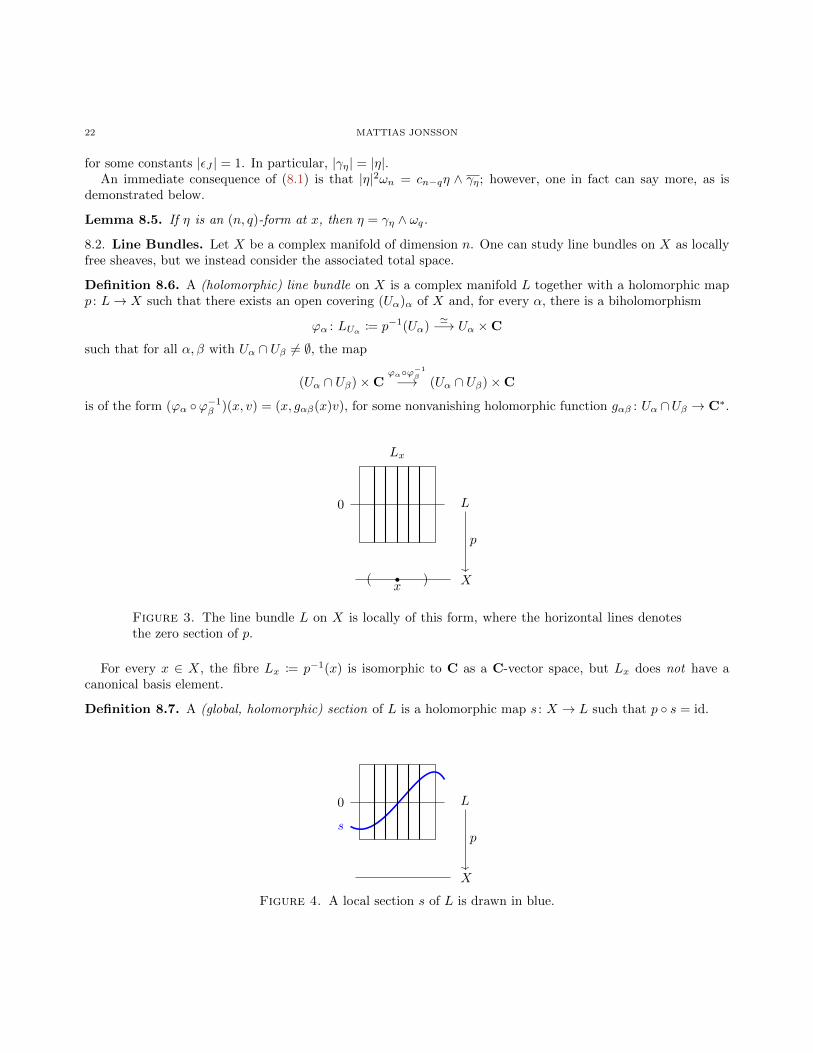
Definition 8.6. A (holomorphic) line bundle on X is a complex manifold L together with a holomorphic mapp : L→ X such that there exists an open covering (Uα)α of X and, for every α, there is a biholomorphism
ϕα : LUα := p−1(Uα)'−→ Uα ×C
such that for all α, β with Uα ∩ Uβ 6= ∅, the map
(Uα ∩ Uβ)×Cϕαϕ−1
β−→ (Uα ∩ Uβ)×C
is of the form (ϕα ϕ−1β )(x, v) = (x, gαβ(x)v), for some nonvanishing holomorphic function gαβ : Uα ∩Uβ → C∗.
0 L
Xx( )
Lx
p
Figure 3. The line bundle L on X is locally of this form, where the horizontal lines denotesthe zero section of p.
For every x ∈ X, the fibre Lx := p−1(x) is isomorphic to C as a C-vector space, but Lx does not have acanonical basis element.
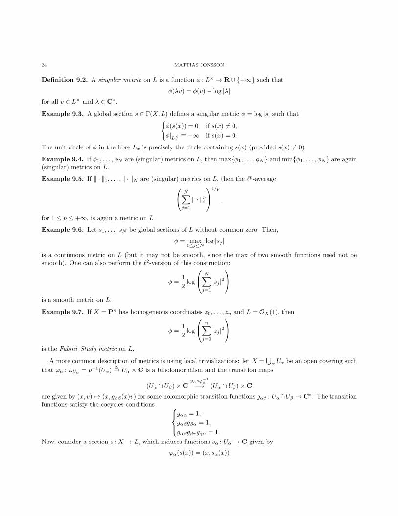
Definition 8.7. A (global, holomorphic) section of L is a holomorphic map s : X → L such that p s = id.
0
s
L
X
p
Figure 4. A local section s of L is drawn in blue.
MATH 710: TOPICS IN MODERN ANALYSIS II – L2-METHODS 23
Example 8.8. The trivial line bundle is L = OX = X × C. The sections of L are precisely the holomorphicfunctions on X.
Example 8.9. The canonical bundle is L = ΩnX , whose sections are the global holomorphic n-forms (equivalently,(n, 0)-forms) on X.
Example 8.10. If X = Pn and m ∈ Z, then there is a family of line bundles L = O(m) whose sections are(holomorphic) homogeneous polynomials of degree m (at least for m ≥ 0).
8.3. Metrics on Line Bundles.
Definition 8.11. A metric on a line bundle L is a function
‖ · ‖ : L→ R+ := [0,+∞)
such that for all x ∈ X, the restriction of ‖ · ‖ to Lx is a norm (on the C-vector space Lx); that is, for all v ∈ Lx,
• ‖v‖ = 0 iff v = 0;• for all λ ∈ C, ‖λv‖ = |λ| · ‖v‖.
Equivalently, ‖ · ‖ determines the unit circle in every fibre Lx of L (though it still does not specify a basis!).
This is a very weak definition, since there is no relation between the fibres. This is often referred to as aFinsler metric on the line bundle.
Definition 8.12. A metric ‖ · ‖ is smooth/continuous/upper semicontinuous (usc)/lower semicontinuous (lsc)if for any local nonvanishing section s : U → L (defined on an open subset U ⊆ X), the function
x 7→ ‖s(x)‖
is smooth/continuous/usc/lsc.
9. January 24th
9.1. Metrics on Line Bundles (Continued). Let X be a complex manifold, and let p : L → X be a linebundle. Last time, we introduced the multiplicative version of a metric on L: a function
‖ · ‖ : L −→ R+ = [0,+∞)
such that the restriction ‖ · ‖|Lx is a vector space norm for all x ∈ X.For various purposes, it is more convenient to look at the additive version of a metric: φ :− − log ‖ · ‖. That
is, the metric φ is now thought of as a function
φ : L× −→ R,
where L× = L\zero section (if one wishes to include the zero section, one must allow φ to take the value +∞).The function φ has the property that
φ(λv) = φ(v)− log |λ|for v ∈ L and λ ∈ C∗.
The choice of a metric ‖ · ‖ or φ on L is equivalent to the choice of a unit circle ‖ · ‖ = 1 = φ = 0 in eachfibre Lx of L.
Example 9.1. A metric on OX = X ×C is equivalent to the data of a R-valued function on X: given a metricφ : O×X = X ×C∗ → R, define a function χ : X → R by the formula
χ(x) = φ(x, 1).
Conversely, given a function χ, set
φ(x, λ) = χ(x)− log |λ|.
24 MATTIAS JONSSON
Definition 9.2. A singular metric on L is a function φ : L× → R ∪ −∞ such that
φ(λv) = φ(v)− log |λ|for all v ∈ L× and λ ∈ C∗.
Example 9.3. A global section s ∈ Γ(X,L) defines a singular metric φ = log |s| such thatφ(s(x)) = 0 if s(x) 6= 0,
φ|L×x ≡ −∞ if s(x) = 0.
The unit circle of φ in the fibre Lx is precisely the circle containing s(x) (provided s(x) 6= 0).
Example 9.4. If φ1, . . . , φN are (singular) metrics on L, then maxφ1, . . . , φN and minφ1, . . . , φN are again(singular) metrics on L.
Example 9.5. If ‖ · ‖1, . . . , ‖ · ‖N are (singular) metrics on L, then the `p-average N∑j=1
‖ · ‖pi
1/p
,
for 1 ≤ p ≤ +∞, is again a metric on L
Example 9.6. Let s1, . . . , sN be global sections of L without common zero. Then,
φ = max1≤j≤N
log |sj |
is a continuous metric on L (but it may not be smooth, since the max of two smooth functions need not besmooth). One can also perform the `2-version of this construction:
φ =1
2log
N∑j=1
|sj |2
is a smooth metric on L.
Example 9.7. If X = Pn has homogeneous coordinates z0, . . . , zn and L = OX(1), then
φ =1
2log
n∑j=0
|zj |2
is the Fubini–Study metric on L.
A more common description of metrics is using local trivializations: let X =⋃α Uα be an open covering such
that ϕα : LUα = p−1(Uα)'→ Uα ×C is a biholomorphism and the transition maps
(Uα ∩ Uβ)×Cϕαϕ−1
β−→ (Uα ∩ Uβ)×C
are given by (x, v) 7→ (x, gαβ(x)v) for some holomorphic transition functions gαβ : Uα∩Uβ → C∗. The transitionfunctions satisfy the cocycles conditions
gαα = 1,
gαβgβα = 1,
gαβgβγgγα = 1.
Now, consider a section s : X → L, which induces functions sα : Uα → C given by
ϕα(s(x)) = (x, sα(x))
MATH 710: TOPICS IN MODERN ANALYSIS II – L2-METHODS 25
for x ∈ Uα. The compatibility/transition rules give that
sα = gαβsβ
on Uα ∩ Uβ .Define local sections eα : Uα → LUα = p−1(Uα) by the formula
ϕα(eα(x)) = (x, 1)
for x ∈ Uα. Now, similar to the case of sections, a metric φ can be described using functions φα : Uα → R, whereφα := φ eα. One can check that
eα = g−1αβeβ ,
φα − φβ = log |gαβ |(9.1)
on Uα∩Uβ . Thus, one can equivalently define a metric φ on L to be a family (φα) of R-valued function satisfyingthe compatibility condition (9.1).
9.2. Operations on Line Bundles and Metrics.
9.2.1. Mappings. If X,Y are complex manifolds, f : Y → X is a holomorphic map, and L is a line bundle on X,then M := f∗L is a line bundle on Y .
L
x = f(y)
Lx
XyY
M
f
My
Figure 5. The pullback line bundle M = f∗L of L.
Given a trivializing cover (Uα) of X and transition function gαβ of L, then (f−1(Uα)) is a trivializing coverof Y and transitions functions gαβ f of M .
If φ is a metric on L corresponding to the family (φα) of R-valued functions on the cover (Uα), then ψ := f∗φis a metric on L given by the family (ψα = φα f) on the cover (f−1(Uα)) of Y .
Example 9.8. If Y → X is an open subset of a closed submanifold, then the pullback of the line bundle issimply the restriction of the line bundle.
Example 9.9. If Y → X = Pn is a closed embedding, then we will often be interested in pulling back L = OX(1)with the Fubini–Study metric.
9.2.2. Tensor Products. If L′ and L′′ are line bundles on X, then L := L′⊗L′′ is a line bundle on X with fibres
Lx = L′x ⊗C L′′x
as (1-dimensional) vector spaces over C. In terms of transition functions, if (g′αβ) and (g′′αβ) are the transition
functions of L′ and L′′ respectively, thengαβ = g′αβ · g′′αβ
are the transition functions of L. We will sometimes use the additive notation L′ + L′′ := L′ ⊗ L′′ (this is notto be confused with the direct sum of line bundles, which would be a vector bundle of higher rank).
26 MATTIAS JONSSON
Now, if φ′ and φ′′ are metrics on L′ and L′′ respectively, then φ = φ′ + φ′′ is a metric on L with localdescription given by
φα = φ′α + φ′′α.
In particular, if φ is a metric on L and χ is a function onX (viewed as a metric onOX in the sense of Example 9.1),then φ+χ is a metric on L. (Conversely, any other metric on L can be obtained from φ from a function on X.)
9.2.3. Inverses. If L is a line bundle on X with transition functions (gαβ), then −L := L−1 is a line bundle on
X with transition functions (g−1αβ ). Similarly, if φ is a metric on L given by the local functions (φα), then −φ
denotes the metric on −L given by the local function (−φα).
9.3. The Curvature Form. Let φ be a smooth (really, C2) metric on a line bundle L onX, which is locally givenby the function (φα) satisfying φα − φβ = log |gαβ | on Uα ∩Uβ , and the transition function gαβ : Uα ∩Uβ → C∗
are holomorphic and non-vanishing. This implies that log |gαβ | is pluriharmonic, i.e.
∂ ∂ log |gαβ | = 0 (9.2)
as a (1, 1)-form on Uα ∩ Uβ .
Definition 9.10. The curvature form of the metric φ is the (1, 1)-form ddcφ that is locally given by
ddcφ := ddcφα =i
π∂ ∂ φα
on Uα. This is well-defined precisely because of (9.2).
Remark 9.11. The normalization in Definition 9.10 of ddcφ is such that the de Rham cohomology class of ddcφin H2(X,R) is equal to the (first) Chern class c1(L) of L.
Definition 9.12. The metric φ is positive if ddcφ is a positive form, which is the pointwise condition on theholomorphic tangent spaces T 1,0
x X thatddcφ(v, v) > 0
for all v ∈ T 1,0x X. Equivalently, this means that the local functions φα are strictly plurisubharmonic for all α:
in local coordinates (z1, . . . , zn), we haven∑
j,k=1
i∂2 φα∂ zj ∂ zk
(x)wjwk > 0
for all x and all w ∈ Cn\0.
Example 9.13. The Fubini–Study metric on Pn is positive.
10. January 26th
10.1. Kahler Manifolds. Let X be a complex manifold.
Definition 10.1. A Kahler form on X is a smooth, positive, closed (1, 1)-form ω (where closed means thatdω = 0, or equivalently ∂ ω = 0 and ∂ ω = 0). We say that (X,ω) (or simply X) is a Kahler manifold.
Example 10.2. If L is a line bundle on X and φ is a smooth, positive, metric on L, then ω := ddcφ = iπ ∂ ∂ φ
is a Kahler form.
Example 10.3. [The Fubini–Study metric/form on Pn] If X = Pn has homogeneous coordinates z0, . . . , zn andL = OX(1), then the Fubini–Study metric on L is given by
φ :=1
2log
n∑j=0
|zj |2 .
MATH 710: TOPICS IN MODERN ANALYSIS II – L2-METHODS 27
In terms of the standard cover X =⋃nj=0 Uj , where Uj = zj 6= 0 ' Cn: on Uj , use coordinates ξi = zi
zjfor
i 6= j and trivializing sections ej = zj , then
φ = log |zj |+1
2log
1 +∑i 6=j
|ξi|2
︸ ︷︷ ︸=φj
,
where we view log |zj | as a metric on O(1)|Uj , and φj as a function on Uj . One can check that φi−φj = log |zj/zi|,where gij = zj/zi are the transition functions.
Claim 10.4. φ is a positive metric.
The claim implies that ω := ddcφ is a Kahler form on X = Pn, called the Fubini–Study form.
Sketch. Consider the function Φ = 12 log
(∑nj=0 |zj |2
)on Cn+1\0 ' L×. It suffices to check that ddcΦ > 0
except along lines thru 0. By the U(n + 1)-invariance of Φ, it suffices to look at the point (z0, . . . , zn) =(1, 0, . . . , 0). Observe that
∂ Φ
∂ zj=
1
2
zj∑ni=0 |zi|2
and
∂2 Φ
∂ zj ∂ zk=
−12
zj zk
(∑ni=0 |zi|2)
2 , j 6= k
12
1−|zj |2
(∑ni=0 |zi|2)
2 , j = k
Thus, at (1, 0, . . . , 0), we get that
ddcΦ =1
2π
n∑j=1
idzj ∧ d zj .
This completes the proof of the claim.
In particular, Pn is a Kahler manifold.
Example 10.5. As a consequence of Example 10.3, any quasiprojective manifold is Kahler: take an embeddingX → Pn and take ω to the pullback of the Fubini–Study form on Pn. (The converse is not true: there areKahler manifolds that do not arise as complex algebraic varieties, e.g. a ‘generic’ complex torus Cn/Λ.)
Example 10.6. Continuing Example 10.3 in the case of P1, we can use the coordinate ξ = ξ1 = z1z0
on C ⊆ P1
to write the Fubini–Study form as
ω =1
2ddc log
(1 + |ξ|2
)=
i
2π
dξ ∧ dξ(1 + |ξ|2)2
.
One can check (in polar coordinates) that∫P1 ω = 1.
10.2. Forms with Values in a Line Bundle. Let X be a complex manifold, and let L be a line bundle on Xwith transitions functions gij corresponding to trivializations (ϕi, Ui, ei).
Definition 10.7. A (p, q)-form η with coefficients in L is a section of the (complex3) vector bundle Λp,q ⊗L onX. More concretely, η is given locally by ηi ⊗ ei, where ηi is a (p, q)-form on Ui, and they satisfy ηi = gijηj .
3This is is a complex, but not holomorphic, vector bundle on X because the transition functions are only smooth in general.
28 MATTIAS JONSSON
Now, fix a (smooth) metric φ on L (corresponding to R-valued functions φi on Ui), then
|η|e−φ := |ηi|e−φ
is a well-defined global function on X, sinceφi − φj = log |gij |,ei = g−1
ij · ej .
If ω is a Kahler (or any positive) form on X, then one can define the L2-norms of (p, q)-forms with values in L:
‖η‖2 :=
∫X
|η|2e−2φdVω,
where dVω is the volume form ωn = ωn
n! . (For example, if φ is a positive metric, then one could take ω = ddcφ.)There are additional global objects that one can associate to L-valued forms:
• If ξ, η are L-valued (p, q)-forms, then 〈ξ, η〉e−2φ is a global function on X, where 〈ξ, η〉 is the pointwiseinner-product.• If ξ, η are L-valued forms, then ξ ∧ ηe−2φ is a global form on X (but it is no longer L-valued); locally,
it is given by
ξi ∧ ηie−2φi ,
and notice that there are no ei’s present in the above expression.
One can also define ∂ on (p, q)-forms (or any forms, really) with values in L: locally, write such a form asη = ηi ⊗ ei, and set
∂ η := ∂ ηi ⊗ ei.This is well-defined since ηi = gijηj , so
∂ ηi = gij ∂ ηj
because the gij ’s are holomorphic. However, there is no d-operator of ∂-operator, unless ∂ gij = 0 (however, if
∂ gij = 0 and ∂ gij = 0, then the gij ’s are constant, which is not very interesting).We can now state a (non-optimal version) of Hormander’s theorem that we will later try to prove.
Theorem 10.8. [Hormander’s Theorem – Non-Optimal Version] Let X be a compact Kahler manifold of di-mension n, let L be a line bundle with a positive metric φ, so ω := ddcφ is a Kahler form on X. Fix q > 0.Given a ∂-closed (n, q)-form f with values in L, then there exists a (n, q − 1)-form u with values in L such that∂ u = f and ∫
X
|u|2e−2φdVω = ‖u‖2 ≤ 1
q‖f‖2,
provided that the right-hand side is finite.
The method of proof will be similar to the more classical versions of Hormander’s theorem: we need tounderstand the adjoint of ∂ and prove a ‘basic identity’. In order to have an adjoint, we need an additionalconstruction called the Chern connection.
10.3. The Chern Connection. Recall that we cannot define ∂ η when η is a form with values in a line bundleL. However, given a smooth metric φ on L, there is the Chern connection, which is a rule
D : L-valued forms of degree r −→ L-valued forms of degree r + 1
satisfying some natural conditions. In our situation, there is a decomposition
D = ∂+δ,
MATH 710: TOPICS IN MODERN ANALYSIS II – L2-METHODS 29
where δ is an operator of bidegree (1, 0) (just as for ∂) and, locally, satisfies
δ (ηi ⊗ ei) =(e2φ ∂ e−2φiηi
)⊗ ei
= (−2 ∂ φi ∧ ηi + ∂ ηi)⊗ ei.
Said differently, δ is a “twisted version” of ∂.
Exercise 10.9. The operator δ is globally-defined.
Exercise 10.10. If ξ, η are forms with values in L, then
∂(η ∧ ξe−2φ
)= ∂ η ∧ ξe−2φ + (−1)∂(η)η ∧ δξe−2φ.
Exercise 10.11. We have the identities ∂2
= 0 and δ2 = 0.
Exercise 10.12. The curvature D2 of the Chern connection D can be expressed as
D2 = δ ∂+ ∂ δ = 2 ∂ ∂ φ = −2πiddcφ,
i.e. we have D2η = 2 ∂ ∂ φ ∧ η for any L-valued form η.
11. January 29th
The goal of today’s class is to work towards the basic identity in the geometric setting. First, we recall thenotation that was established in the previous class.
Let (X,ω) be a Kahler manifold of dimension n, let L be a line bundle on X, and let φ be a smooth metricon L. In terms of local data, if there is an open cover X =
⋃i Ui over which L is trivialized with transition
functions gij , then L has local sections ei and φ is given by functions φi. These satisfy the transition rulesei = g−1
ij ej ,
φi = φj + log |gij |.
Furthermore, an L-valued form η on X is given by the local data η = ηi ⊗ ei, where the ηi’s are local formssatisfying ηi = gijηj .
There are standard operations that can be performed on these forms with values in a line bundle, which aresummarized below:
• if ξ, η are L-valued (p, q)-forms, then 〈ξ, η〉e−2φ is a function on X;• if ξ, η are L-valued forms, then ξ ∧ ηe−2φ is a form on X;• if η is an L-valued form, then ∂ η := ∂ ηi ⊗ ei and
δη :=(e2φi ∂ e−2φiηi
)⊗ ei
= (−2 ∂ φi ∧ ηi + ∂ ηi)⊗ ei.
There are two important formulas satisfied by the ∂ and δ operators:
∂(η ∧ ξe−2φ
)= ∂ η ∧ ξe−2φ + (−1)deg(η)η ∧ δξe−2φ, (11.1)
(δ ∂+ ∂ δ)η = 2 ∂ ∂ φ ∧ η. (11.2)
30 MATTIAS JONSSON
11.1. The Formal Adjoint of ∂. The formal adjoint of ∂, denote ∂∗φ, is an operator that should satisfy the
identity ∫X
〈∂ η, ξ〉e−2φdVω =
∫X
〈η, ∂∗φ ξ〉e−2φdVω, (11.3)
where η is an L-valued (n, q− 1)-form of compact support, and ξ is an L-valued (n, q)-form. We will express ∂∗φ
using the ∗-operator, which sends an (n, q)-form ξ to an (n− q, 0)-form γξ. Recall that there was an equality
〈∂ η, ξ〉e−2φdVω = cn−q ∂ η ∧ γξe−2φ
of (n, n)-forms on X, which one can verify locally. In particular, the left-hand side of (11.3) can be expressed as
cn−q
∫X
∂ η ∧ γξe−2φ = cn−q
∫X
∂ (η ∧ γξ) e−2φ − (−1)n−q+1cn−q
∫X
η ∧ δγξe−2φ (11.4)
where the first equality holds by (11.1). Note that
∂ (η ∧ γξ) e−2φ = 0
for degree reasons (indeed, it is an (n + 1, n− 1)-form on the n-dimensional manifold X, and hence it is zero);thus, it follows that ∫
X
∂ (η ∧ γξ) e−2φ = 0
by Stokes’ formula. Similarly, the integrand on the right-hand side of (11.3) can be written as
〈η, ∂∗φ ξ〉e−2φdVω = cn−q+1η ∧ γ∂∗φ ξe−2φ.
Now, one can check that
cn−q+1 = i(n−q+1)2
cn−q = i(n−q)2
=⇒ cn−q+1 = (−1)n−qcn−q · i
Putting these together, one finds that
i
∫X
η ∧ δγξe−2φ =
∫X
η ∧ γ∂∗φ ξe−2φ (11.5)
for all test forms η. We conclude that
γ∂∗φ ξ= iδγξ . (11.6)
From this formula4, one can get a local description for the formal adjoint ∂∗φ, but really we will only require (11.6).
11.2. Positivity of Forms. The reference for this material is [Dem12, III.1]. Let V be a C-vector space ofdimension n (which we will later take to be the tangent space to X at a point). The exterior power of V ∗C, whichis a 2n-dimensional C-vector space, admits a decomposition
ΛV ∗C =⊕p,q≤n
Λp,qV ∗,
where Λp,qV ∗ is the vector subspace of (p, q)-forms.
4The formula (11.6) might be off by a minus sign.
MATH 710: TOPICS IN MODERN ANALYSIS II – L2-METHODS 31
11.2.1. Positivity of (n, n)-Forms. As C-vector spaces, we have an isomorphism Λn,nV ∗ ' C. Given (linear)
which is a (real) (n, n)-form. Note that, for another choice of coordinates w, τ transforms as
τ(w) = τ(z) ·∣∣∣∣det
(∂ wj∂ zk
)∣∣∣∣2 . (11.7)
We say that an (n, n)-form u is positive if there exists c ≥ 0 such that u = c · τ(z). (In particular, with thisdefinition, the zero (n, n)-form is positive.) By (11.7), this definition of positivity is independent of the choiceof coordinates z.
11.2.2. Positivity of (p, p)-Forms. Given a (p, p)-form u, the following are equivalent:
(1) u|W ≥ 0 for any p-dimensional C-linear subspace W ⊆ V ;(2) u ∧ iα1 ∧ α1 ∧ . . . ∧ iαn−p ∧ αn−p ≥ 0 for any (1, 0)-forms α1, . . . , αn−p.
We say u is positive if (1) and (2) hold.
Fact 11.1.
(1) A (1, 1)-form i∑j,k ujkdzj ∧ d zk is positive iff the corresponding Hermitian form
ξ 7→∑j,k
ujkξjξk
is semipositive definite.(2) If α is a (p, 0)-form, then cpα ∧ α is a positive (p, p)-form.(3) If α is a positive (p, p)-form and β is a positive (1, 1)-form, then α ∧ β is a positive (p+ 1, p+ 1)-form.
While (3) holds, be warned that it is not true in general that the wedge of two positive forms is again positive.
11.3. The Basic Identity. Given a smooth (n, q)-form α with values in L, set
Tα := cn−qγn−q ∧ γn−q ∧ ωq−1e−2φ,
which is a positive (n− 1, n− 1)-form (with values in OX). Note that
Tα ∧ ω = qcn−qγn−q ∧ γn−q ∧ ωqe−2φ
= q|γα|2e−2φdVω
= q|α|2e−2φdVω,
where the final equality follows from the fact that α 7→ γα is an isometry.
Theorem 11.2. [Basic Identity] For an (n, q)-form α with values in L, we have
i ∂ ∂ Tα =(−2Re
⟨∂ ∂∗φ α, α
⟩+ | ∂ γα|2 + | ∂∗φ α|2 − | ∂ α|2
)e−2φdVω + 2i ∂ ∂ φ ∧ Tα (11.8)
as (n, n)-forms on X.
The proof of the basic identity is not difficult - it is simply an integration by parts argument (which we maydiscuss next time). Integrating (11.8) gives the following, important corollary.
Corollary 11.3. If α has compact support (e.g. if X is compact), then
2
∫X
i ∂ ∂ φ ∧ Tα +
∫X
| ∂ γα|2e−2φdVω =
∫X
| ∂ α|2e−2φdVω +
∫X
| ∂∗φ α|2e−2φdVω. (11.9)
32 MATTIAS JONSSON
Proof. By Stokes’ formula,∫X∂ ∂ Tα = 0, and we have∫
X
〈∂ ∂∗φ α, α〉e−2φdVω =
∫X
| ∂∗φ α|2e−2φdVω
by the definition of the adjoint. Thus, (11.9) follows just from integrating (11.8).
Granted Corollary 11.3, if one knows that 2i ∂ ∂ φ ≥ cω, then one obtains an estimate of the form∫X
| ∂ α|2e−2φdVω +
∫X
| ∂∗φ α|2e−2φdVω ≥ c∫X
Tα ∧ ω = cq
∫X
|α|2e−2φdVω,
which will be a good starting point in order to apply L2-methods similar to the ones previously introduced.
12. January 31st
Recall the notation from last time: (X,ω) is a Kahler manifold of dimension n, L is a line bundle on X, andφ is a metric on L. If η is an L-valued (n, q)-form, then γη is an L-valued (n− q, 0)-form satisfying η = γη ∧ ωq,as well as the identities
where the last equality follows since γα ∧ ωq = α, and the second-to-last equality follows since dω = 0. Substi-tuting these two formulas into (12.4) gives (12.1).
By dropping the second term on the left-hand side of (12.1), one gets an obvious corollary of the basic identity.
Corollary 12.2. If α is a smooth (n, q)-form with compact support, then
2
∫X
i ∂ ∂ φ ∧ Tα ≤∫X
| ∂ α|2e−2φdVω +
∫X
| ∂∗φ α|2e−2φdVω. (12.5)
Corollary 12.3. If i ∂ ∂ φ ≥ cω for some positive constant c > 0 (in particular, φ is a positive metric), then∫X
| ∂ α|2e−2φdVω +
∫X
| ∂∗φ α|2e−2φdVω ≥ 2cq
∫X
|α|2e−2φdVω. (12.6)
34 MATTIAS JONSSON
Proof. The inequality i ∂ ∂ φ ≥ cω means that one can write i ∂ ∂ φ = cω + β, where β is a positive (1, 1)-formon X. The positivity of Tα and β (and that β is of bidegreee (1, 1)) implies that β ∧Tα is a positive (n, n)-form;in particular,
∫Xβ ∧ Tα ≥ 0. Also, we have∫
X
ω ∧ Tα =
∫X
ω ∧ cn−qγα ∧ γα ∧ ωq−1e−2φ
= q
∫X
cn−qγα ∧ γα ∧ ωqe−2φ
= q
∫X
cn−qα ∧ γαe−2φ
= q
∫X
|α|2e−2φdVω.
Combining the above expression with (12.5) immediately gives (12.6).
12.2. Setup for the Hilbert Space Machinery. Consider the sequence of closed and densely-defined opera-tors
H1T=∂−→ H2
S=∂−→ H3,
where
H2 =
L-valued (n, q)-forms α with L2
loc-coefficients such that ‖α‖2 :=
∫X
|α|2e−2φdVω
,
and the Hilbert spaces H1 and H3 are defined similarly, with (n, q− 1) and (n, q+ 1)-forms respectively. Corol-lary 12.3 gives the bound
‖T ∗α‖2 + ‖Sα‖2 ≥ 2cq‖α‖2
for all smooth, compactly-support α, and we must extend the bound to all forms α ∈ DT∗ ∩DS . This does notwork in general! (For example, if X = U ⊆ Cn is an open subset, L = OX , and φ is strictly psh, then we mustassume that U is pseudoconvex!).
The methods works when
• X is compact;• (X,ω) is a complete Kahler manifold (i.e. the associated Riemannian metric on X is complete);• (X,ω) is Kahler, and X admits some other complete Kahler metric.
The method used to tackle the final condition is analogous to the approach we used to prove Hormander’stheorem for a pseudoconvex domain in Cn.
The goal of next class is to discuss the approxmation result required to make the above method work.
Theorem 12.4. [Approximation Lemma] Assume that X is compact, and α is an L-valued (n, q)-form.
(1) if α is smooth, then α ∈ DT∗ ∩DS and T ∗α = ∂∗φ α;
(2) if α ∈ DT∗ ∩DS, then there exists a sequence (αk)∞k=1 of L-valued smooth forms such that
‖αk − α‖, ‖Sαk − Sα‖, ‖T ∗αk − T ∗α‖ −→ 0 as k → +∞.
The idea of the proof of the approximation lemma is to use convolution, which we will outline next time.
13. February 2nd
13.1. The Proof of Hormander’s Theorem on Compact Kahler Manifolds. The goal of today’s class isto complete the proof of Hormander’s theorem in the geometric setting, which we recall below.
MATH 710: TOPICS IN MODERN ANALYSIS II – L2-METHODS 35
Theorem 13.1. [Hormander’s Theorem] Let (X,ω) be a compact Kahler manifold of dimension n, let L be aline bundle on X, and let φ be a metric on L such that
2i ∂ ∂ φ ≥ cω.Given an (n, q)-form f with values in L such that ∂ f = 0, then one can solve ∂ u = f with the estimate∫
X
|u|2e−2φdVω ≤1
cq
∫X
|f |2e−2φdVω,
provided the right-hand side is finite.
Last time, we proved the basic identity, from which we deduced the corollary below.
Corollary 13.2. [Of the Basic Identity] With notation as in Theorem 13.1, for any L-valued (n, q)-form α (withcompact support), we have
c‖α‖2 ≤ ‖ ∂ α‖2 + ‖ ∂∗φ α‖2.
Consider the seq uence
H1T=∂−→ H2
S=∂−→ H3
where H1 consists of (n, q − 1) forms, H2 consists of (n, q)-forms, and H3 consists of (n, q + 1)-forms.
Theorem 13.3. [Approximation Lemma] Assume X is compact and α ∈ H2.
(1) If α is smooth, then α ∈ DT∗ ∩DS and T ∗α = ∂∗φ α.
(2) If α ∈ DS ∩DT∗ , then there exists a sequence (αk)∞k=1 of smooth (n, q)-forms such that
‖αk − α‖, ‖Sαk − Sα‖, ‖T ∗αk − T ∗α‖ −→ 0 as k → +∞.
Proof. For (1), it is clear that α ∈ DS . Moreover, the statement that α ∈ DT∗ and T ∗α = ∂∗φ α means that∫
X
〈∂ u, α〉e−2φdVω =
∫X
〈u, ∂∗φ α〉e−2φdVω
for all u ∈ DT (and a form u lies in DT if u ∈ H1 and ∂ u, computed in the sense of distributions, lies in H2).This equality holds by the definition of the distributional derivative (because α is a test form).
For (2), we will only sketch the argument. We first prove that for α ∈ DS ∩DT∗ and χ ∈ C∞(X) (either realor complex-valued), then χα ∈ DS ∩DT∗ . That χα ∈ DS is easy, since
∂ (χα) = ∂ χ ∧ α+ χ∂ α
in the sense of distributions. Further, one must check that χα ∈ DT∗ : this amounts to showing that there existsa constant C > 0 such that
|〈∂ u, χα〉H2| ≤ C‖u‖H1
for all u ∈ DT . Observe that
〈∂ u, χα〉H2=
∫X
〈∂ u, χu〉e−2φdVω
= 〈χ∂ u, α〉H2
= 〈∂(χu), α〉H2 − 〈∂ χ ∧ u, α〉H2 .
As u ∈ DT (hence χu ∈ DT ) and α ∈ DT∗ , it follows from the above equality that there are constants C,C ′ > 0such that
|〈∂(χu, α〉H2| ≤ C‖χu‖H1
≤ C ′‖u‖H1
and|〈∂ χ ∧ u, α〉H2 | ≤ C‖u‖H1 ,
where the last equality follows by the Cauchy–Schwarz inequality. We conclude that χα ∈ DS ∩DT∗ .
36 MATTIAS JONSSON
Now, we can use a partition of unity (ψj) to write α =∑j ψjα and we can approximate each term. Thus,
we can assume WLOG that α has support in a coordinate chart z : U → Cn where L|U is trivial. We cannow use convolutions: pick χ : Cn → R with compact support and
∫Cn
χ = 1, and set χk(z) := k2nχ(kz) andαk := α ∗ χk. Thus, it follows from the general properties of convolution that
‖αk − α‖ −→ 0 as k → +∞.
However, we also need to show that ‖Sαk − Sα‖ → 0 and ‖T ∗αk − T ∗α‖ → 0 as k → +∞. For S = ∂, this isok because S has constant coefficients, i.e. we have
∂(α ∗ χk) = ∂ α ∗ χk.Therefore, the same argument gives that ‖Sαk − Sα‖ → 0 as k → +∞. For T ∗, one must be more carefulbecause it does not have constant coefficents; indeed, when n = 1, recall that
∂∗φ(fdz) =
∂ f
∂ z− 2
∂ φ
∂ zf.
To conclude the estimate for T ∗, one must use Friedrich’s lemma; see [Dem12, VIII,3.3]. This concludes the(sketch of the) proof of the approximation lemma.
13.2. Hormander’s Theorem on Noncompact Kahler Manifolds. Let (X,ω) be a Kahler manifold ofdimension n and we no longer assume that X is compact. Let L and φ be as before; in particular, we have theestimate
2i ∂ ∂ φ ≥ cωon the curvature of φ. Then, the statement of Hormander’s theorem is the same, assuming X admits some othercomplete Kahler metric ω′.
Example 13.4. This condition is satisfied when X is a Stein manifold (e.g. a pseudoconvex open subset of Cn).
Granted this additonal assumption, the proof of Hormander’s theorem is as follows:Step 1. Assume ω′ = ω, so ω is complete. Use this to prove the density of test forms in DS ∩DT∗ .Step 2. Apply Step 1 for (X,ω+k−1ω′) (which is possible since ω+k−1ω′ remains complete for k ∈ Z>0), and
solve ∂ uk = f with estimates. Then, one shows that uk → u, which is a solution with the required estimates.
13.3. Relation to Kodaira’s Theorems.
Theorem 13.5. [The Kodaira Vanishing Theorem] If X is compact of dimension n and L is a positive linebundle on X (i.e. there exists φ such that i ∂ ∂ φ > 0), then the Dolbeault cohomology satisfies
Hn,q(X,L) = 0
for q > 0.
Remark 13.6. The algebro-geometric incarnation of Kodaira’s vanishing theorem says that if X is projectiveand L is ample, then Hq(X,KX + L) = 0 for q > 0.
Theorem 13.5 is almost a consequence of Hormander’s theorem, except the solution u to the equation ∂ u = fis a priori not smooth. One can either modify the approach in the proof of Hormander’s theorem to guaranteeu is smooth (but one loses the estimates), or one can use Hodge theory. Hodge theory shows that each element
of Hn,q(L) is represented by a harmonic form α, i.e. ∆α = (∂∗φ ∂+ ∂ ∂
∗φ)α = 0. This occurs iff ∂ α = ∂
∗φ α = 0.
The Laplacian ∆α is a zeroth-order elliptic operator, so one can use strong results from the theory of ellipticPDE’s; in particular, we can use the estimate
0 = ‖ ∂ α‖2 + ‖ ∂∗φ α‖2 ≥ ‖α‖2
where the norms are taken with respect to the Kahler form ω := 2i ∂ ∂ φ. It is thus clear that, if ∂ α = 0 and
∂∗φ α = 0, then α = 0.
From Theorem 13.5, we can deduce another important result due to Kodaira.
MATH 710: TOPICS IN MODERN ANALYSIS II – L2-METHODS 37
Theorem 13.7. [Kodaira Embedding Theorem] If X is compact and there exists a positive line bundle L onX, then X is projective, i.e. there exists a closed embedding X → PN
C .
Idea of Proof of Theorem 13.7. For m 0, given a basis s0, . . . , sNm of holomorphic sections of ωX ⊗ Lm (i.e.global holomorphic n-forms with values in Lm), define a meromorphic map
X 99K P(H0(X,ωX ⊗ Lm)∗
)given by x 7→ [s0(x) : . . . : sNm(x)], and one checks that this map is well-defined (i.e. holomorphic), injective,and that is separates 1-jets.
We will just explain the first property: given x ∈ X, we must find a (global) holomorphic n-form s withvalues in L such that s(x) 6= 0. The idea is to construct s as s = η−u, where η is a locally-defined smooth format x (with some additional properties) and u is a solution to ∂ u = ∂ η (so that ∂ s = 0) with estimates thatguarantee u(x) = 0 and η(x) 6= 0.
14. February 5th
Let (X,ω) be compact Kahler manifold of dimension n, let L be a line bundle on X, and let φ be a smoothmetric on L such that 2i ∂ ∂ φ ≥ εω. In this setting, we completed the proof of Hormander’s theorem, whichasserts the following: for any L-valued (n, q)-form f such that ∂ f = 0 and
∫X|f |2e−2φdVω < +∞, then there
exists an L-valued (n, q − 1)-form u such that ∂ u = f and with the estimate∫X
|u|2e−2φdVω ≤1
εq
∫X
|f |2e−2φdVω.
14.1. Smoothness of Solutions. In Hormander’s theorem, one can always pick the solution u to have minimalnorm (though there is not a unique such u), and this condition is equivalent to demanding that u ∈ ker(∂)⊥.Now, assume that f is smooth and u is a minimal solution to ∂ u = f . One can consider the Laplace operator
∆ := ∂∗φ ∂+ ∂ ∂
∗φ,
thought of as an operator on the space of (n, q − 1)-forms with values in L. As u ∈ ker(∂)⊥ = im(∂∗φ), we have
∂∗φ u = 0; in particular,
∆u = (∂∗φ ∂+ ∂ ∂
∗φ)u = ∂
∗φ,
which is smooth. It follows from elliptic regularity that u is smooth.
14.2. The Kodaira Embedding Theorem (Continued). We continue the proof of Kodaira’s embeddingtheorem (Theorem 13.7), which we began last time. Let X be compact and let L be a positive line bundle. Fixm 1. Given x ∈ X, construct global holomorphic Lm-valued (n, 0)-forms on X that do not vanish at x (wherem is chosen independent of x). This gives rise to a holomorphic map
X −→ P(H0(X,ωX ⊗ Lm)∗
).
The construction of such sections is discussed below.Pick a (smooth) positive metric φ on L, and consider the Kahler form ω := 2i ∂ ∂ φ. Pick open neighbourhoods
V b W b U of x such that there exists a coordinate chart z : U → Cn with z(x) = 0 and L|U is trivial. Pickχ ∈ C∞(X) such that 0 ≤ χ ≤ 1, supp(χ) ⊆ U , and χ ≡ 1 on W . Given δ > 0, set
ψδ(y) := (n+ 1)χ(y)) · 1
2log(|z(y)|2 + δ2
).
Then, ψδ ∈ C∞(X), supp(ψδ) ⊆ U , δ 7→ ψδ is increasing, and
limδ→0
ψδ(y) = (n+ 1)χ(y) log |z(y)| = ψ0(y)
38 MATTIAS JONSSON
has a singularity at y = x (indeed, it is −∞ there and we understand its growth as y → x). Furthermore,i ∂ ∂ ψδ ≥ 0 on W (i.e. on the locus where χ ≡ 1). We want to “add” ψδ to the metric φ and apply Hormander’stheorem with the resulting metric.
Pick m 1 and ε > 0 such that
2i ∂ ∂ (mφ+ ψδ) ≥ εω (14.1)
for every δ ∈ (0, 1), where mφ + ψδ is thought of as a metric on Lm. (In addition, the estimate (14.1) can bemade uniform in x.) Pick a holomorphic section σ of L|U and assume that σ(x) 6= 0 (this is possible since L|Uis trivial, so one can e.g. take a trivialization). Set
η := χ · σmdz1 ∧ . . . ∧ dzn,
which is a smooth (but not holomorphic) Lm-valued (n, 0)-form on X with supp(η) ⊆ U and ∂ η = 0 on W (i.e. onthe locus where χ ≡ 1). Set f := ∂ η, which is a smooth Lm-valued (n, 1)-form on X such that supp(f) ⊆ U\Wand ∂ f = 0.
Now, use Hormanders’ theorem to get uδ, which is an Lm-valued (n, 0)-form on X such that ∂ uδ = f = ∂ ηand with the estimate ∫
X
|uδ|2e−2(mφ+ψδ)dVω ≤1
ε
∫X
|f |2e−2(mφ+ψδ)dVω, (14.2)
The right-hand side of (14.2) is bounded above by some constant C > 0 that is independent of δ. We want totake u = limδ→0 uδ, but we must be careful about the sense in which this limit is taken. If we set
Hδ :=
v :
∫X
|v|2e−2(mφ+ψδ)dVω < +∞,
then there are inclusions Hδ → Hδ′ for δ < δ′. By a diagonal argument and weak compactness (by the Banach–Alaoglu theorem), there exists a sequence δj 0 and u ∈
⋂j Hδj such that ‖u‖Hδj ≤ C for all j and uδj → u
weakly in Hδj for all j; thus, uδj → u in the sense of distributions, hence ∂ uδj → ∂ u in the sense of distributions.
It follows that ∂ u = f .Set s := η − u, then ∂ s = ∂ η − ∂ u = f − f = 0 in the sense of distributions. However, if the (n, 0)-form s
with values in Lm satisfies ∂ s = 0 in the sense of distributions, then s is holomorphic. In particular, u is smooth(because η is smooth) and it is holomorphic on W . However, we also have the estimates∫
X
|u|2e−2(mφ+ψδj )dVω ≤ C (14.3)
for all j, so the monotone convergence theorem implies that there is the estimate∫X
|u|2e−2(mφ+ψ0)dVω ≤ C. (14.4)
Rewrite e−2ψ0(y) = |z(y)|−(n+1) for y in the neighbourhood W of x, which is not locally integrable at x.Therefore, the only way that (14.4) can hold is if u(x) = 0, and hence s(x) 6= 0, as required.
14.3. The Ohsawa–Takegoshi Theorem. The next goal of the class is to discuss the extension theorem ofOhsawa–Takegoshi, which originates in [OT87] and it has since been generalized in many different directions.Later, we will focus on the geometric version of the extension theorem, but we will begin with the function-theoretic version.
Consider a bounded, pseudoconvex domain U ⊆ Cn (so there is a “good supply” of holomorphic functions onU , for example a polydisc), and fix a hyperplane H ⊆ Cn such that U ∩H 6= ∅.
Question 14.1. Given a holomorphic function on f on U ∩H, does there exist F on U such that F |U∩H = f?
The Ohsawa–Takegoshi theorem asserts that the answer to Question 14.1 is yes, and this can be done withestimates.
MATH 710: TOPICS IN MODERN ANALYSIS II – L2-METHODS 39
Theorem 14.2. [Ohsawa–Takegoshi Theorem] There exists a constant C = C(U,H) > 0 such that given any(smooth) φ ∈ PSH(U) and f ∈ O(U ∩H) such that
∫U∩H |f |
2e−2φ < +∞, then there exists F ∈ O(U) such thatF |U = f and with the estimate ∫
U
|F |2e−2φ ≤ C∫U∩H
|f |2e−2φ.
The key point is that the constant C is independent of both φ and f . Note that all of the integrals appearingin Theorem 14.2 are taken with respect to Lebesgue measure on the appropriate subset of Cn.
Geometrically, it is more natural to look at (n, 0)-forms, in which case “restriction” means to apply thePoincare residue map (i.e. the map appearing in the adjunction formula “KX +H|H ' KH”).
15. February 7th
15.1. The Ohsawa–Takegoshi Extension Theorem in the Unit Disc. The simplest, nontrivial case ofthe Ohsawa–Takegoshi extension theorem takes places in the unit disc, where we are attempting to construct aholomorphic function with a specific value at (say) the origin and satisfying an appropriate integral estimate.
Theorem 15.1. There exists a universal constant C > 0 such that for all φ ∈ SH(D) ∩ C∞(D), there existsh ∈ O(D) such that h(0) = 1 and ∫
D
|h|2e−2φdV ≤ Ce−2φ(0) (15.1)
The assumption that φ be smooth is not necessary, but we add this first for simplicity. The main point isthat C does not depend on φ, which means that one can derive the result for any φ ∈ SH (D), which is no longerassumed to be smooth.
Moreover, one can specify that h have any value at the origin 0 (or at any point in D), provided one adds afactor of |h(0)|2 to the right-hand side of (15.1).
There are alternate versions of Theorem 15.1, where one replaces (15.1) with the sharper result∫D
|h|2
(|z| log |z|)2 e−2φdV ≤ C|h(0)|2e−2φ(0).
This inequality is still not optimal, but we will later proceed to the geometric setting, instead of optimizing theclassical setting.
Remark 15.2. There is an “adjoint version” of Theorem 15.1, where one replaces h by h(z)dzz , but it is thesame estimate.
We will follow Berndtsson’s approach in [Ber10]. The idea is to write h = u · z, where u solves (in the senseof distributions) the equation
∂ u
∂ z= δ0
with suitable estimates, where δ0 denotes the Dirac mass at 0.
15.2. Distributions & Currents in C. Use the coordinate z = x+ iy on C, and pick a Kahler form
ω :=i
2dz ∧ d z = dz ∧ dy = dV.
Consider the space5 D := D(C) = C∞0 (C) of test functions on C, and the space D′ of distributions on C is theset of continuous linear functional on D. There is an obvious embedding D ⊆ L1
loc, as well as an embeddingL1
loc → D′ given by
α 7→(β 7→
∫C
αβdV
).
Operations on D′ are defined to commute with the embedding D → D′, and a few of these are illustrated below:
5The topology on D is the Frechet topology where we demand that all possible derivatives converge on all compact subsets.
40 MATTIAS JONSSON
• Differentiation: if u ∈ D′ and α ∈ D, then 〈∂ u∂ z , α〉 := −〈u, ∂ α∂ z 〉, and similarly for ∂ u∂ z .
• Multiplication: if u ∈ D′ and α, β ∈ D, then 〈αu, β〉 := 〈u, αβ〉.These are the main two operations that we will use.
For 0 ≤ p, q ≤ 1, let D(p,q) be the set of test (p, q)-forms on C, and the space D′(p,q) of currents of bidegree
(p, q) is defined to be the set of continuous linear functions on D(1−p,1−q) (often, we say that the elements ofD′(p,q) are of bidimension (p, q)). Similar to the case of distributions, there is an embedding D(p,q) → D′(p,q)given by
α 7→(β 7→
∫C
α ∧ β).
There are natural operations that one can define on currents:
• Wedge Product : if T ∈ D′(1−p−r,1−q−s), α ∈ D(p,q), β ∈ D(r,s), then 〈T ∧ α, β〉 := 〈T, α ∧ β〉.• Differentiation: define ∂ : D′(p,q) → D′(p+1,q) by the formula
〈∂ T, α〉 := (−1)p+q+1〈T, ∂ α〉,
and similarly one defines ∂ : D′(p,q) → D′(p,q+1). From ∂ and ∂, set d := ∂+ ∂ and dc := i2π (∂− ∂), and
the Laplacian-type operator ddc = iπ ∂ ∂.
One can realize currents as “forms with distribution-coefficients” as follows: consider the isomorphism
D′(0,0)'−→ D′
given by
T 7→ (α 7→ 〈T, αdV 〉) .Similarly, D′(1,0) ' D
′dz, D′(0,1) ' D′d z, and D′(1,1) ' D
′dz ∧ d z via analogous isomorphism.
Lemma 15.3. Computed in D′, we have the equalities
∂
∂ z
1
z=
∂
∂ z
1
z= πδ0.
Proof. Use the Cauchy integral formula: if Ω ⊆ C is open and bounded with ∂ Ω consisting of finitely-manyJordan curves (i.e. we are able to integrate along the boundary), then
u(ξ) =1
2πi
∫∂ Ω
u(z)
z − ξdz +
1
2πi
∫Ω
∂ u∂ z
z − ξdz ∧ d z (15.2)
for all u ∈ C1(Ω) (i.e. u is the restriction of a C1-function on an open neighbourhood of Ω); see the first chapterof [H90]. Now, if α ∈ D, then
〈 ∂∂ z
1
z, α〉 = −〈1
z,∂ α
∂ z〉
= −∫C
1
z
∂ α
∂ z
= − i2
∫C
1
z
∂ α
∂ zdz ∧ d z
= − i2· 2πiα(0)
= πα(0),
where the second-to-last equality follows from Cauchy’s integral formula (15.2). Notice that, since α has compactsupport, we can take all of the integrals to be over some large disc containing the origin.
Corollary 15.4. Computed in D′(1,1), we have ddc log |z| = δ0.
MATH 710: TOPICS IN MODERN ANALYSIS II – L2-METHODS 41
For most purposes (as in Corollary 15.4), it is convenient to think of measures as currents of maximal bidegree.In fact, Corollary 15.4 is a special case of the more general Poincare–Lelong formula.
Proof. Write log |z| = 12 log(z z) so that
ddc log |z| = i
2π∂ ∂ log(z z) =
i
2π∂
(1
zd z
)=
i
2ππδ0dz ∧ d z = δ0 · dV.
Fact 15.5. If u ∈ D′ satisfies ∂ u∂ z = 0, then u is holomorphic (in particular, it is a C∞-function).
This is a simple case of a more general phenomenon known as elliptic regularity, and it also follows fromWeyl’s lemma (which is the analogous fact for (real) harmonic functions).
15.3. The Ohsawa–Takegoshi Extension Theorem in the Unit Disc (Continued). Recall that we mustconstruct h ∈ O(D) such that h(0) = 1 and satisfying the L2-estimate∫
D
|h|2e−2φdV ≤ Ce−2φ(0).
Consider the following heuristics: suppose h exists and write h = u · z for some u ∈ L1loc ⊆ D′, which implies
that ∂ u∂ z = πδ0 in D′. If α ∈ D(D), then this formally gives
πα(0)e−2φ(0) =
∫D
∂ u
∂ zαe−2φdV
=
∫D
u
(∂
∂ z
)∗αe−2φdV
=
∫D
h
(∂∂ z
)∗α
ze−2φdV,
where(∂∂ z
)∗denotes a suitable adjoint operator. Using the Cauchy–Schwarz inequality to estimate this last
integral, we find that
π2|α(0)|2e−4φ(0) ≤(∫
D
|h|2e−2φdV
)︸ ︷︷ ︸
≤Ce−2φ(0)
∫D
∣∣∣( ∂∂ z )∗ α∣∣∣2|z|2
e−2φdV
.
Simplifying, this implies that
|α(0)|2e−2φ(0) ≤ C
π2
∫D
∣∣∣( ∂∂ z )∗ α∣∣∣2|z|2
e−2φdV (15.3)
for all α ∈ D(D). There is one problem with this, namely that |z|−2 is not locally integrable, so this last integralwill often be +∞, and so (15.3) may not have much content to it.
The idea is to prove a modified version of the estimate (15.3), and then use the Hahn–Banach theorem andthe Riesz representation theorem in order to reconstruct a holomorphic function h with the desired properties.
42 MATTIAS JONSSON
16. February 9th
16.1. The Ohsawa–Takegoshi Extension Theorem in the Unit Disc (Continued). Recall that the goalis to show the following: there exists a constant C > 0 such that for all φ ∈ SH(D) ∩ C∞(D), there existsh ∈ O(D) such that h(0) = 1 and with the estimate
∫D
|h|2e−2φdV ≤ Ce−2φ(0). (16.1)
We will prove this with C = 8π, which is larger than the optimal constant C = π.The proof, like the proof of Hormander’s theorem, uses the Hilbert space approach. We will work with
(OX -valued) forms, as opposed to functions. Fix the Kahler form
ω :=i
2dz ∧ d z = dV,
so the norms of dz and d z with respect to this metric are |dz| = |d z | =√
2. For α ∈ D(1,1)(D) = D(1,1), write
α = γ∧ω, where γ = γα ∈ D is such that α = i2γdz∧d z. As before, we have operators ∂ and δ = δφ = e2φ ∂ e−2φ
on such forms.
Proposition 16.1. There exists r < 1 and C = Cr > 0 such that for all test functions γ ∈ D,
|γ(0)|2e−2φ(0) ≤ C∫D
|δγ|2
|z|2re−2φdV. (16.2)
Proposition 16.1 implies the Ohsawa–Takegoshi Theorem. Set
V :=
δγ
|z|r: γ ∈ D
⊆ L2
(1,0)(φ),
and Proposition 16.1 implies that δγ|z|r 7→ γ(0)e−φ(0) is a bounded antilinear functional on V of norm ≤
√C. By
the Hahn–Banach theorem and the Riesz representation theorem, there exists η = ηr ∈ L2(1,0)(φ) such that
∫D
|η|2e−2φdV ≤ C (16.3)
and
γ(0)e−φ(0) =
∫D
〈η, δγ|z|r〉e−2φdV =
∫D
η ∧ δγ
|z|re−2φ (16.4)
for all γ ∈ D. Set u = ur := η|z|r e
−φ(0) ∈ L1(1,0)(loc) ⊆ D′(1,0). Now, (16.3) and (16.4) imply that
∂ u = δ0,∫D|u|2|z|2re−2φ ≤ Ce−2φ(0).
(16.5)
MATH 710: TOPICS IN MODERN ANALYSIS II – L2-METHODS 43
Let us check the equality ∂ u = δ0 of currents more carefully: any test function can be written as γe−2φ for sometest function γ, and so we can check
〈∂ u, γe−2φ〉 = −〈u, ∂(γe−2φ
)〉
= −∫D
u ∧ ∂(γe−2φ)
= −∫D
u ∧ ∂(γe−2φ)
= −∫D
u ∧ δγe−2φ
= −e−φ(0)
∫D
η ∧ δγ
|z|re−2φ
= γ(0)e−2φ(0),
and hence ∂ u = δ0 as currents on D.Now, set β = 2πizu ∈ D′(1,0), then ∂ β = 2πiz ∂ h = 2πiz · δ0 = 0 in the sense of distributions, so Fact 15.5
implies that β is holomorphic; thus, we can write β = hdz for some holomorphic function h. Observe that∂(hdzz
)= 2πiδ0, so h(0) = 1 because ∂
(dzz
)= 2πiδ0. Furthermore,∫
D
|h|2e−2φdV =
∫D
|β|2e−2φdV = 4π2
∫D
|z|2|u|2e−2φdV
≤ 4π2
∫D
|z|2r|u|2e−2φdV
≤ 4π2Ce−2φ(0),
where the last inequality follows from (16.5).
We will prove Proposition 16.1 with the constant C = Cr = 2πr , which gives the final constant of 8π in the
Ohsawa–Takegoshi estimate (16.1).
Proof of Proposition 16.1. We will use the “basic identity”: set T := c0γ ∧ γ ∧ ω0e−2φ = |γ|2e−φ, which is a
function on D, where c0 = 1 and ω0 = 1. Then, the smooth (1, 1)-form i ∂ ∂ T can be written as
i ∂ ∂ T = 2Im((∂ δγ
)· γe−2φ
)+ 2i
(∂ ∂ φ
)· T︸ ︷︷ ︸
≥0
+(| ∂ γ|2 + |δγ|2
)e−2φdV︸ ︷︷ ︸
≥0
,
where the second term is non-negative by the subharmonicity of φ. Thus, we will use the inequality
i ∂ ∂ T ≥ 2Im((∂ δγ
)· γe−2φ
). (16.6)
Now, set w = −r log |z| and W = 1 − e−w, so w ≥ 0 and 0 ≤ W ≤ 1. Multiplying (16.6) by w, integrating,using the Cauchy–Schwarz inequality gives one estimate; repeating the same thing for W gives another estimate;finally, combining these two estimates completes the proof. This proof will be explained in more detail nexttime.
17. February 12th
There will be no class on Friday the 16th and Monday the 19th.
44 MATTIAS JONSSON
17.1. The Ohsawa–Takegoshi Extension Theorem in the Unit Disc (Continued). Recall the versionof the Ohsawa–Takegoshi theorem in the unit disc D that we are in the midst of proving:
Theorem 17.1. [Ohsawa–Takegoshi] For any φ ∈ SH(D) ∩ C∞(D), there exists h ∈ O(D) such that h(0) = 1and satisfying the estimate ∫
X
|h|2e−2φdV ≤ 8πe−2φ(0).
Last time, we reduced the proof of Theorem 17.1 to the following proposition.
Proposition 17.2. For all r < 1 and all γ ∈ D := D(D), we have
|γ(0)|2e−2φ(0) ≤ 2
πr
∫X
|δγ|2
|z|2re−2φdV
Proposition 17.2 implies Theorem 17.1. By the Hahn–Banach theorem and the Riesz representation theorem,there exists η = ηr ∈ L1
(1,0)(φ) such that ∫X
|η|2e−2φdV ≤√
2
πr, (17.1)
and
γ(0)e−φ(0) =
∫X
iη ∧ δγ
|η|re−2φ. (17.2)
Now, (17.2) implies that u := ie−φ(0)
|z|r η satisfies ∂ u = δ0 in D′(1,1); this means that, when paired against any test
function (which can be written as γe−2φ), we have
〈∂ u, γe−2φ〉 = 〈u, ∂(γe−2φ
)〉
= 〈u, ∂(γe−2φ)〉
= 〈u, δγe−2φ〉
=
∫X
u ∧ δγe−2φ
= e−φ(0)
∫X
iη
|z|r∧ δγe−2φ
= γ(0)e−2φ(0),
where the final equality follows from (17.2). Granted the formula ∂ u = δ0, if we set β := 2πizu = hdz ∈ D′(1,0),
then it satisfies ∂ β = 0, so ∂ h = 0 and h(0) = 1. Now, (17.1) implies that∫X
|h|2e−2φdV ≤ 4π2 2
πre−2φ(0),
and one can send r → 1− to conclude.
Recall that the pointwise inner product on (1, 0)-forms satisfies the formula 〈ξ, η〉e−2φ = iξ ∧ ηe−2φ; that is,γξ = ξ in this case.
Proof of Proposition 17.2. The first step is to write the ‘basic identity’: if T := |γ|2e−2φ, then
i ∂ ∂ T = 2Im((∂ ∂ γ
)· γe−2φ
)+ 2i ∂ ∂ φ · T +
(| ∂ γ|2 + |δγ|2
)e−2φdV, (17.3)
which, when combined with the subharmonicity of φ, gives the inequality
i ∂ ∂ T ≥ 2Im((∂ ∂ γ
)· γe−2φ
). (17.4)
MATH 710: TOPICS IN MODERN ANALYSIS II – L2-METHODS 45
Multiplying (17.4) by the non-negative function w := −r log |z| and integrating over D yields the inequality∫X
i ∂ ∂ T · w ≥ 2Im
∫X
∂ δγ · γwe−2φ. (17.5)
By thinking of w as a current, the left-hand side of (17.5) can be rewritten as the pairing of currents
〈w, i ∂ ∂ T 〉 = 〈i ∂ ∂ w, T 〉 = −πrT (0) = −πr|γ(0)|2e−2φ(0).
To compute the right-hand side of (17.5), we want to use Stokes’ theorem, so observe that
d(δγ · γwe−2φ
)= ∂
(δγ · γwe−2φ
)= ∂ δγ · γwe−2φ − δγ ∧ δ(γw)e−2φ (17.6)
where the first equality follows for degree reasons. Using the Leibnitz formula, the second term on the right-handside of (17.6) can be computed as
δ(γw)e−2φ = δ(γw)e−2φ = δγ · we−2φ + γ(∂ w)e−2φ.
Thus, the right-hand side of (17.5) can be rewritten as
2Im
∫X
∂ δγ · γwe−2φ = 2Im
∫X
δγ ∧ δ(γw)e−2φ
= 2Im
∫X
δγ ∧ δγwe−2φ + 2Im
∫X
δγ ∧ γ(∂ w)e−2φ
= −2
∫X
|δγ|2we−2φdV + 2Im
∫X
δγ ∧ γ(∂ w)e−2φ
where the first equality follows from Stokes’ formula. Therefore, (17.5) implies that
πr|γ(0)|2e−2φ(0) ≤ 2
∫X
|δγ|2we−2φdV − 2Im
∫X
δγ ∧ γ(∂ w)e−2φ (17.7)
Now, applying the Cauchy–Schwarz inequality to the last term of (17.7), we get that
−2Im
∫X
δγ ∧ γ(∂ w)e−2φ = −2Im
∫X
ewδγ ∧ e−wγ(∂ w)e−2φ
≤∫X
e2w|δγ|2e−2φdV +
∫X
e−2w|γ|2| ∂ w|2e−2φdV.
Combining the above inequality with (17.7) yields
πr|γ(0)|2e−2φ(0) ≤∫X
(e2w + 2w
)|δγ|2e−2φdV +
∫X
e−2w|γ|2| ∂ w|2e−2φdV. (17.8)
The first term of the right-hand side of (17.8) is essentially want we want, because e2w = 1|z|2r , so we must deal
with the second term. This is done via a trick, where one redoes the same arguments as above, but with adifferent weight function.
Consider the function W := 1− e−2w, so 0 ≤W ≤ 1. Then,∂ W = e−2w ∂ w in D′(0,1),
i ∂ ∂ W = −4e−2w| ∂ w|2dV in D′(1,1).(17.9)
The proof of these equalities is left as an exercise. Now, we want to repeat the previous procedure with Winstead of w: this gives the inequality∫
X
i ∂ ∂ T ·W ≥ 2Im
∫X
∂ ∂ γ · γWe−2φ (17.10)
46 MATTIAS JONSSON
and (17.9) implies that the left-hand side of (17.10) is
−4
∫X
e−2w|γ|2| ∂ w|2e−2φdV,
whereas the right-hand side of (17.10) can (using Stokes’s theorem) be written as
−2
∫X
|δγ|2We−2φdV + 2Im
∫X
δγ ∧ γ(∂ W )e−2φ.
Thus, (17.10) can be rewritten as
4
∫X
e−2w|γ|2| ∂ w|2e−2φdV ≤ 2
∫X
|δγ|2We−2φdV − 2Im
∫X
δγ ∧ γ(∂ W )e−2φ. (17.11)
Now, use the Cauchy–Schwarz inequality on the last term of (17.11) to get
−2Im
∫X
δγ ∧ γ(∂ W )e−2φ ≤∫X
|δγ|2e−2φdV +
∫X
|γ|2| ∂ W |2e−2φdV
=
∫X
|δγ|2e−2φdV +
∫X
|γ|2e−2w| ∂ w|2e−2φdV,
where the last equality follows from (17.9). Combining this inequality with (17.11) gives the inequality
3
∫X
e−2w|γ|2| ∂ w|2e−2φdV ≤∫X
(2W + 1)︸ ︷︷ ︸≤3
|δγ|2e−2φdV. (17.12)
Finally, combining (17.8) and (17.12) gives the inequality
πr|γ(0)|2e−2φ(0) ≤∫X
(e2w + 2w + 1)|δγ|2e−2φdV ≤∫X
2e2w|δγ|2e−2φdV,
where the second inequality follows from the convexity of the exponential function, i.e. ex ≥ x+ 1. Rearranging,we find that
πr|γ(0)|2e−2φ(0) ≤ 2
∫X
e2w|δγ|2e−2φdV = 2
∫X
|δγ|2
|z|2re−2φdV,
as required.
17.2. Preview of the Geometric Version of the Ohsawa–Takegoshi Theorem. Let us quickly explainthe ingredients and players involved in the geometric version of the Ohsawa–Takegoshi extension theorem, whichwill be our next goal.
Let X be a compact Kahler manifold of dimension n (or perhaps one does not assume compactness), letY ⊆ X be a smooth hypersurface, L is a positive line bundle on X, and let φ be a smooth, positive metric onL. Given an L-valued (n − 1, 0)-form u on Y , we want to find an L + OX(Y )-valued (n, 0)-form U on X suchthat PRY (U) = u and some estimates hold, where PRY denotes the Poincare residue map on Y .
To formulate this precisely, one needs a metric ψ on the line bundle OX(Y ) and the assumptions in thetheorem will involve e.g. the usual semipositivity condition i ∂ ∂ φ > 0 and an estimate of the form
i ∂ ∂ φ ≥ c · i ∂ ∂ ψ.
This second estimate is a new geometric restriction on the extension problem (for example, it depends on thepositivity of the normal bundle of Y in X).
Next time, we will aim to formulate one of the many versions of the geometric Ohsawa–Takegoshi theorem.
18. February 14th
There will be no class on Friday the 16th and Monday the 19th.
MATH 710: TOPICS IN MODERN ANALYSIS II – L2-METHODS 47
18.1. Geometric Version of the Ohsawa–Takegoshi Theorem. Let X be a complex manifold of dimensionn, Y ⊆ X be a smooth hypersurface, and L be a holomorphic line bundle on X. Let ωX be the canonicalline bundle on X, i.e. the line bundle whose local sections are holomorphic (n, 0)-forms. We are interestedin the adjoint line bundles ωX ⊗ L, whose local sections are L-valued (n, 0)-forms, as well as the line bundleωX ⊗ L⊗OX(Y ), whose local sections are L-valued (n, 0)-forms with at at most simple pole along Y .
There is the Poincare residue map ResY : ωX ⊗L⊗OX(Y )→ ωY ⊗L, which is a higher-dimensional versionof taking the residue of a differential form in the complex plane. We want to consider the an extension problemrelated to the residue map:
Problem 18.1. Does the Poincare residue map ResY induce a surjective map
H0(X,ωX ⊗ L⊗OX(Y ))→ H0(Y, ωY ⊗ L|Y )
on global sections?
This extension problem can be considered in the algebro-geometric setting: X is a projective manifold andwe identify ωX = OX(KX) for a canonical divisor KX on X, then there is an exact sequence
0→ OX(KX + L)→ OX(KX + L+ Y )→ OY (KY + L|Y )→ 0
of sheaves in either of the Zariski or analytic topologies, and the associated long exact sequence on cohomologyis of the form
Thus, if H1(X,OX(KX + L)) vanishes, then the extension problem has a positive solution; for example, theKodaira vanishing theorem implies that H1(X,OX(KX + L)) = 0 when L is ample.
18.2. The L2-Extension Problem. We are interested in the following L2-version of Problem 18.1.
Problem 18.2. Given u ∈ H0(Y, ωY ⊗L|Y ), can we find U ∈ H0(X,ωX ⊗L⊗OX(Y )) such that ResY (U) = uand with the estimate
‖U‖ ≤ C‖u‖,where C is some ‘controlled’ constant? Here, ‖U‖ and ‖u‖ are measured in some L2-norms.
We will consider the L2-extension problem in various geometric situations:
(1) X and Y are compact.(2) X ⊆ Cn is a (bounded) pseudoconvex domain (e.g. a ball); in this case, OX(Y ) is a trivial line bundle
(as is ωX), so the statement simplifies.(3) p : X → D is a proper submersion (so p is locally diffeomorphic to a product, but not holomorphically-so)
and the fibres Xt := p(t), for t ∈ D, are compact complex manifolds and we set Y := X0; that is, we areextending sections from the central fibre to the whole family.
The situation (3) is relevant for Siu’s proof of the deformation invariance of plurigenera.To proceed further, we must specify the data needed to define L2-norms on the various spaces of sections, i.e.
we want norms on H0(X,ωX ⊗ L⊗OX(Y )) and H0(Y, ωY ⊗ L|Y ). This is ok if we have the following data:
• a Kahler form ω on X, which gives rise to a volume form dVω = ωn = ωn
n! ;• a metric φ on L;• a metric ψ on OX(Y );• a metrics χ on ωX and χ′ on ωY .
Given this data, we can define
‖u‖2 =
∫Y
|u|2e−2(χ′+φ)dVω
and
‖U‖2 =
∫X
|U |2e−2(χ+φ+ψ)dVω.
48 MATTIAS JONSSON
However, we do not need χ, χ′ nor ω, for the reason that we are working with (n, 0)-forms valued in various linebundles (from such forms, we can ‘cook up’ a volume form).
Remark 18.3. [Metrics on the Canonical Bundle] If X is a complex manifold of dimension n, there is a one-to-one correspondence
metrics on ωX ↔ volume forms on X,where here we think of volume forms on X as positive (n, n)-forms on X. Given a volume form dV on X, wedefine a metric on ωX as follows: given a local nowhere-vanishing section η of ωX (i.e. an (n, 0)-form that is alocal frame of ωX), then cnη ∧ η is a positive (n, n)-form, so it can be written as
cnη ∧ η = h · dV,where h > 0 is a (local) function on X (h is defined on the same domain as η), and we set
‖η‖ :=√h.
Here, we adopt the multiplicative notation for metrics, i.e. the metric is a function ‖ ·‖ : ωX → R≥0. Conversely,given a metric ‖ · ‖ on ωX , define a volume form dV by the formula
dV =cnη ∧ η‖η‖1/2
for any local frame η of ωX .
Now, if η is a (local) L-valued (n, 0)-form on X (not necessarily holomorphic), it is locally given by
η = ηi ⊗ eiwhere the ηi’s transform as ηi = gijηj . If φ is a metric on L, then it is locally given by functions φi thattransform as φi − φj = log |gij |. Then, set
|η|2e−2φ := cnη ∧ ηe−2φ loc= cnηi ∧ ηie−2φi .
This is a well-defined volume form on X. Therefore, we only need a metric φ on L in order to define an L2-norm‖ · ‖ on H0(X,ωX ⊗ L): if η ∈ H0(X,ωX ⊗ L), then set
‖η‖2 :=
∫X
|η|2e−2φ.
To define an L2-norm on H0(X,ωX ⊗L⊗OX(Y )), it suffices to have a metric φ on L and a metric ψ on OX(Y ).With this data, if η ∈ H0(X,ωX ⊗ L⊗OX(Y )), then set
‖η‖X :=
∫X
|η|2e−2(φ+ψ),
where φ+ ψ is viewed as a metric on L⊗OX(Y ).We can now formulate a version of the Ohsawa–Takegoshi extension theorem in the geometric setting.
Theorem 18.4. [Ohsawa–Takegoshi Theorem] Suppose X is a complex manifold (with some restrictions6), Yis a smooth, closed complex hypersurface, s ∈ H0(Y,OX(Y )) is the canonical section such that Y = s = 0, Lis a holomorphic line bundle on X, φ is a smooth metric on L, and ψ is a smooth metric on OX(Y ). Assume
‖s‖ψ ≤ e−1,
ddcφ > 0 (i.e. φ is a positive metric),
ddcφ > ddcψ.
6The restrictions (to be added later) say that X is ‘almost’ a Stein manifold; more precisely, we require that X becomes Steinafter removing a hypersurface.
MATH 710: TOPICS IN MODERN ANALYSIS II – L2-METHODS 49
Then, for any holomorphic section u ∈ H0(Y, ωY ⊗ L|Y ) such that∫Y|u|2e−2φ < +∞, there exists U ∈
H0(X,ωX ⊗ L⊗OX(Y )) such that ResY (U) = u and satisfying the estimate∫X
|U |2e−2(φ+ψ) ≤ C∫Y
|u|2e−2φ, (18.1)
where C > 0 is a universal constant. In fact, one can achieve the stronger estimate∫X
|U |2e−2(φ+ψ)(‖s‖ψ log 1
‖s‖ψ
)2 ≤ C∫Y
|u|2e−2φ. (18.2)
The condition that ‖s‖ψ be bounded is an important technical condition, but the choice of e−1 as upperbound is simply a choice of normalization. Furthermore, the condition ddcφ > ddcψ says roughly that “Y ispositively embedded in X”.
The function(‖s‖ log 1
‖s‖
)−2
on X has a pole along Y = s = 0, but it is integrable in the sense that∫Ω
(‖s‖ log
1
‖s‖
)−2
dV < +∞
for any choice of relatively-compact neighbourhood Ω of Y , i.e Y ⊆ Ω b X and any choice of volume form dVon X. The important point of this discussion is that it is harder to satisfy (18.2) than it is to satisfy (18.1).
19. February 21st
19.1. Geometric Version of the Ohsawa–Takegoshi Theorem (Continued). We recall the rough state-ment of the Ohsawa–Takegoshi theorem that we will aim to prove: let X be a complex manifold (with somerestrictions), Y ⊆ X a (smooth) complex hypersurface, L a holomorphic line bundle on X, φ a smooth metricon L, and ψ a smooth metric on OX(Y ). Assume
|s|ψ ≤ e−1 on X,
ddcφ > 0,
ddcφ > ddcψ,
where s is the canonical section of OX(Y ). Then, for any u ∈ H0(Y, ωY ⊗ L|Y ) such that∫Y|u|e−2φ < +∞,
there exists U ∈ H0(X,ωX ⊗ L⊗OX(Y )) such that ResY (U) = u and satisfying∫X
|U |2e−2(φ+ψ)(|s|ψ log 1
|s|ψ
)2 ≤ C∫Y
|u|2e−2φ,
where C is a purely numeric constant.Said differently, we want to extend sections of ωY ⊗ L|Y to sections of ωX ⊗ L⊗OX(Y ) (with estimates).We will first discuss the necessary assumptions that we must place on X (and on Y ): there exists a (possibly
singular, possibly empty) hypersurface Z ⊆ X such that
• X\Z is Stein;• Z contains no connected component of Y .
The definition of Stein manifolds, which are the complex geometric analogue of affine varieties, is given below.
Definition 19.1. A complex manifold is Stein if it is biholomorphic to a closed submanifold of CN , with N ≥ 1.
Example 19.2. Pseudoconvex domains in Cn are Stein (e.g. the unit ball).
Example 19.3. Below we give various examples of X (and Y ) satisfying the above assumptions:
• if X is a Stein manifold;
50 MATTIAS JONSSON
• if X is a projective manifold, i.e. there is a closed embedding X → PN (in this case, one takes Z = H∩Xfor a (very) general hyperplane H ⊆ PN , which exists by a Bertini theorem).
In the proof of the Ohsawa–Takegoshi theorem (with this assumption on X,Y ), then one can reduce to thecase when X is Stein by passing to X\Z. This is a standard argument (for example, it appears in more generalversions of Hormander’s theorem), but to do so we must discuss another extension problem, namely extensionacross subvarieties. More precisely, we require an L2-version of the Riemann’s Hebbarkeitssatz (i.e. the Riemannextension theorem).
19.2. Extension Across Subvarieties. Let X be a complex manifold, let Z ⊆ X be a (possibly singular)subvariety, and let L be a holomorphic line bundle on X.
Lemma 19.4. Suppose u, f are L-valued forms on X with coefficients in L2(loc) such that ∂ u = f on X\Z (inthe sense of currents). Then, ∂ u = f on X (also in the sense of currents).
Remark 19.5. For applications to the Ohsawa–Takegoshi theorem, we want to take f = 0 in Lemma 19.4;however, for more general versions of Hormander’s theorem, f will be taken to be more general.
Proof. First, assume that Z is smooth. The statement is local, so WLOG we may assume L = OX , X isthe unit ball in Cn, and Z = z′ = 0, where z = (z′, z′′) are coordinates Cn with z′ = (z1, . . . , zm) andz′′ = (zm+1, . . . , zn). Pick a smooth function χ : C→ [0, 1] such that
χ(w) = 0 |w| ≤ 12 ,
χ(w) = 1 |w| ≥ 1.
For 0 < δ < 1, set ξδ := χ(‖z′‖δ
), where ‖z′‖ is (say) the L2-norm on the first m coordinates. The function ξδ
is smooth and it approximates the characteristic function 1X\Z . Note that
• Supp(∂ ξδ
)⊆
12δ ≤ ‖z
′‖ ≤ δ
;• ξδ → 1 as δ → 0− in the sense of distributions; in particular, ξδ · u → u and ξδ · f → f in the sense of
because ξδ ≡ 0 near Z and ∂ u = f on X\Z. As differentiation is continuous on currents, the convergenceξδ · u → u implies that ∂(ξδ · u) → ∂ u; therefore, it suffices to prove that ∂ ξδ ∧ u → 0 in the sense of currentsas δ → 0.
This has no reason to be true in general, since u could blow up very fast as one approaches Z, but now wefinally use the condition that these forms have L2(loc)-coefficients. We must prove that the coefficients of ∂ ξδ∧utend to zero in L1(loc). Granted that
Supp(∂ ξδ
)⊆ ‖z′‖ ≤ δ,∫
‖z′‖≤δ |u|2dV → 0,
where the convergence of the integal follows since u has L2(loc)-coefficients, we can use the Cauchy–Schwartzinequality to say (∫
X
| ∂ ξδ ∧ u|2dV)2
≤
(∫‖z′‖≤δ
|u|2dV
)2(∫‖z′‖≤δ
| ∂ ξδ|2dV
)2
,
MATH 710: TOPICS IN MODERN ANALYSIS II – L2-METHODS 51
so it suffices to prove that supδ∫‖z′‖≤δ | ∂ ξδ|
2dV < +∞. This is fine, since | ∂ ξδ| ≤ Cδ 1‖z′‖≤δ, and hence∫
‖z′‖≤δ| ∂ ξδ|2dV ≤
C2
δ2vol (‖z′‖ ≤ δ) ≤ C ′
δ2δ2m ≤ C ′.
This completes the proof when Z is smooth (in fact, if one does the estimates more carefully, this same argumentcan be used to tackle the singular case).
Finally, suppose that Z is singular. Consider the stratification
Z = Z1 t Z2 t . . . ,
where Z1 := Zreg and Zj+1 = (Zj)reg. (Here, we are using a strong result that says that the regular part of an
analytic set is again analytic.) Now, successively prove that ∂ u = f on X\Zj using the argument above (onemust be careful because the Zj ’s are no longer closed, but only locally closed).
Thus, in the Ohsawa–Takegoshi theorem, we may assume that the complex manifold X is Stein (in fact, thesame holds if we assume that the metrics φ and ψ are slightly singular). This begs the question: why is thisuseful? The answer is in two parts.
(1) In the proof, we start with some extension of u with no estimates and we must modify it to produce U .
Theorem 19.6. [Cartan’s Theorem B] For any analytic coherent sheaf F on a Stein manifold X, theCech cohomology Hp(X,F) vanishes for p ≥ 1.
We will apply Cartan’s Theorem B to F = ωX ⊗ L, which will give the surjectivity of the restrictionmap
H0(X,ωX ⊗ L⊗OX(Y )) H0(Y, ωY ⊗ L|Y ).
(2) If X is Stein, we can exhaust X by relatively compact Stein subdomains (Xn)∞n=1, i.e. satisfying Xn bXn+1 b X. (For example, if X ⊆ AN , then take Xn = X ∩B(0, n).)
20. February 23rd
20.1. Geometric Version of the Ohsawa–Takegoshi Theorem (Continued). We recall the rough state-ment of the Ohsawa–Takegoshi theorem that we will aim to prove: let X be a complex manifold (with somerestrictions), Y ⊆ X a (smooth) complex hypersurface and X,Y is “Stein-able” (in the sense discussed lastclass), L a holomorphic line bundle on X, φ a smooth metric on L, and ψ a smooth metric on OX(Y ). Assume
|s|ψ ≤ e−1 on X,
ddcφ > 0,
ddcφ > ddcψ,
where s is the canonical section of OX(Y ). Then, for any u ∈ H0(Y, ωY ⊗ L|Y ) such that∫Y|u|e−2φ < +∞,
there exists U ∈ H0(X,ωX ⊗ L⊗OX(Y )) such that ResY (U) = u and satisfying∫X
|U |2e−2(φ+ψ)(|s|ψ log 1
|s|ψ
)2 ≤ C∫Y
|u|2e−2φ,
where C is a universal constant.
Reductions. Below we note the reductions that we can make in order to prove the Ohsawa–Takegoshi theorem.
(1) Assume X is Stein (this was explained last time, using the extension of holomorphic forms across
subvarieties). Thus, Cartan’s Theorem B implies that there exists U ∈ H0(X,ωX ⊗ L ⊗ OX(Y )) such
that ResY (U) = u (but with no estimates!).
52 MATTIAS JONSSON
(2) Assume that ∫X
|U |2e−2(φ+ψ)(|s|ψ log 1
|s|ψ
)2 < +∞.
To do this, write X =⋃∞n=1Xn, where Xn is a Stein open subset of X, and Xn b Xn+1. Then,∫
Xn
|U |2e−2(φ+ψ)(|s|ψ log 1
|s|ψ
)2 < +∞
for all n ≥ 1. Set Yn := Y ∩ Xn. Suppose we can find (using some modification of U) some formsUn ∈ H0(X,ωX ⊗ L⊗OX(Y )) such that ResYn(Un) = u|Yn and with the estimates∫
Xn
|Un|2e−2(φ+ψ)(|s|ψ log 1
|s|ψ
)2 ≤ C∫Yn
|u|2e−2φ ≤ C∫Y
|u|2e−2φ.
Then, one can extract a limit (uniformly on compacts) U = limj→+∞
Unj that solves the problem on X.
The idea now is to modify U using a solution to the ∂-equation (this is similar to the part of the proof ofthe Kodaira Embedding Theorem, where we cook up a holomorphic section that does not vanish at a specifiedpoint). To that end, pick a smooth function χ : R→ [0, 1] such that
χ = 0 on [1,+∞),
χ = 1 on (−∞, 12 ].
Set χε := χ(|s|2ψε2
), where s is the canonical section of Y ; χε is a smooth function on X and it is an approximation
of the indicator function 1Y of Y . Now, solve the equation ∂ Vε = ∂(χεU) with suitable estimates so thatVε = 0 on Y (this can be arranged by using a non-integrable weight, as in the proof of the Kodaira Embedding
Theorem7). Then, we will set U := χεU − Vε and this function will be the solution to the extension problem.
20.2. Remarks on Hormander’s Theorem. In order to make the aforementioned strategy work, we will needa slight variant of the version of Hormander’s theorem that we proved. Recall the version that we proved:
Theorem 20.1. [Hormander’s Theorem] If X is (say) Stein of dimension n, L is a (positive) line bundle, ω isa Kahler form, φ is a metric on L such that
2i ∂ ∂ φ ≥ cω,then for any L-valued (n, q)-form f , there exists an L-valued (n, q − 1)-form u such that ∂ u = f and∫
X
|u|2e−2φdVω ≤1
qc
∫X
|f |2e−2φdVω. (20.1)
We will only use Hormander’s theorem in the case q = 1. In this case, one can remove the dependence on ω!First, in the left-hand side of (20.1), we have
|u|2e−2φdVω = cnu ∧ ue−2φ
because u is an L-valued (n, 0)-form. For the right-hand side of (20.1), we require a slight modification of this,which is similar to the dimension-1 estimate of the form∫
D
|u|2e−2φ ≤∫D
|f |2
∆φe−2φ (20.2)
7In the proof of the Kodaira Embedding Theorem, the strategy was to show that∫X |f |
2e−2n log ‖z−z0‖dV < +∞, which implies
f(z0) = 0, since the weight function is non-integrable near z0.
MATH 710: TOPICS IN MODERN ANALYSIS II – L2-METHODS 53
on the unit disc D (or the corresponding estimate on Cn that we saw).Recall the basic identity (for q = 1): if α is a compactly-supported L-valued (n, 1)-form, then∫
X
2i ∂ ∂ φ ∧ Tα +
∫X
| ∂ γα|2e−2φdVω =
∫X
| ∂ α|2e−2φdVω +
∫X
| ∂∗φ α|2e−2φdVω, (20.3)
where γα is now an L-valued (n− 1, 0)-form and Tα = cn−1γα ∧ γαe−2φ is an L-valued (n− 1, n− 1)-form. Here,the second term on the left-hand side of (20.3) is ≥ 0 and we will ignore it, and we will work with α such that∂ α = 0 (so the first term on the right-hand side of (20.3) disappears). Now, the first term of the left-hand sideof (20.3) does not depend on the choice of Kahler form ω, and
| ∂∗φ α|2e−2φdVω = |γ∂∗φ α|2e−2φdVω
= |δγα|2e−2φdVω
= cnδγα ∧ δγαe−2φ,
so the term | ∂∗φ α|2e−2φdVω is also independent of ω! Modifying the L2-method using these observations yieldsthe following result:
Theorem 20.2. Given X,L, φ as above, one can solve ∂ u = f with the estimate∫X
|u|2e−2φdVω ≤∫X
fθ · e−2φ, (20.4)
provided the right-hand side is finite, and θ is the Kahler form := 2i ∂ ∂ φ. (Further, the left-hand side of (20.4)is independent of ω.)
The right-hand side of (20.4) is the analogue of the 1-dimesional estimate (20.2). To see this is just someHermitian algebra: working pointwise, the Kahler form θ := 2i ∂ ∂ φ is a positive (1, 1)-form and it defines aHermitian inner product on Λp,q for all p, q (in particular, on Λ1,1). Taking the pairing with θ gives a linearfunction
Λ1,1 (·,θ)−→ C.
This induces a map
Λn,1 ⊗ Λ1,n '−→ Λ1,1 ⊗ Λn,n(·,θ)−→ Λn,n,
i.e. the target consists of volume forms! There is also an L-valued version, given a metric φ: given an L-valued(n, 1)-form f , write fθ · e−2φ for the image of if ⊗ fe−2φ under the map above.
Remark 20.3. [Minimal Solutions] If u is a solution to ∂ u = f and u ⊥ ker(∂), then u is the solution withminimum norm (indeed, up to these only being densely-defined, any solution can be decomposed as the minimalsolution plus an element of ker(∂), and the norms only increase upon adding an element of ker(∂)). Thus, umust satisfy (20.4).
21. March 5th
21.1. Geometric Version of the Ohsawa–Takegoshi Theorem (Continued). The plan is to finish theproof of this version of the Ohsawa–Takegoshi theorem by the next class. Afterwards, we will probably starttalking about invariance of log plurigenera, which will be an application of this theorem.
Theorem 21.1. [Ohsawa–Takegoshi] Let X be a complex manifold and let Y ⊂ X be a smooth analytic hy-persurface (and the pair (X,Y ) is “Steinable”, in the sense of the previous class). Let L be a holomorphic linebundle on X, and let φ and ψ be smooth metrics on L and OX(Y ), respectively. Assume that |s|ψ ≤ e−1 on X,
54 MATTIAS JONSSON
and that ddcφ > 0 and ddcφ > ddcψ. Then, for all u ∈ H0(Y, ωY ⊗L|Y ) such that∫Y|u|2e−2φ <∞, there exists
U ∈ H0(X,ωX ⊗ L⊗OX(Y )) such that ResY U = u and∫X
|U |2e−2(φ+ψ)
(|s|ψ log 1|s|ψ )2
≤ C∫Y
|u|2e−2φ
where C is a universal constant and |s|ψ = |s|e−ψ.
The statement says that you can extend an L-valued top form on Y to an L-valued top form on X, with someestimates. The argument is a bit technical; the statement and proof is from lecture notes [Bou17] by Boucksom.
21.1.1. Reductions So Far. We have reduced to the case when X is Stein, in which case we already know that
there exists U ∈ H0(X,ωX ⊗ L⊗OX(−Y )) such that ResY U = u and∫X
|U |2e−2(φ+ψ)
(|s|ψ log 1|s|ψ )2
<∞.
Note, however, that we have no estimates. The point is then to “correct” U using the ∂-equation, as follows.Pick a C∞ function χ : R→ [0, 1] such that
χ ≡ 0 on [1,∞]
χ ≡ 1 on [−∞, 12 ]
Then, χε := χ(|s|2ψε2 ) is a C∞ function on X that approximates 1Y , where we recall that s is the canonical section
of OX(Y ) such that s = 0 = Y . We then want to solve ∂ Vε = ∂(χεU) with estimates on Vε that force
Vε|Y = 0. If Uε := χεU − Vε, then suitable estimates will show that limε→0 Uε = U works.
21.1.2. Reduction To A Twisted Hormander Estimate. Suppose we can solve the ∂-equation
∂ Vε = ∂(χεU) = ε−2χ′( |s|2ψε2
)∂(|s|2ψ) ∧ U , (21.1)
with an estimate ∫X
|Vε|2|s|−2ψ
(log 1|s|ψ+ε )
2 e−2(φ+ψ) ≤
∫supp ∂ Vε
|U |2|s|−2ψ e−2(φ+ψ) (21.2)
where the constant C is a purely numerical constant. Then, the fact that the left-hand side of (21.2) is finiteforces Vε = 0 on Y (i.e., ResY Vε = 0). Now using (21.1), we have
supp ∂ Vε ⊂ε
2≤ |s|ψ ≤ ε
(21.3)
and the volume of this set is roughly ε2. This would imply that the right-hand side of (21.2) satisfies
limε→0
∫supp ∂ Vε
|U |2|s|−2ψ e−2(φ+ψ) ≤ C
∫Y
|u|2e−2φ (21.4)
by the fact that ResY U = u. Using (21.2) and (21.4), we can take a weak limit (in L2) as ε → 0: Setting
Uε := χεU − Vε, we have that ∂ Uε = 0 hence Uε ∈ H0(X,ωX ⊗ L⊗OX(Y )), and ResY Uε = u. Now
limε→0
∫X
|χεU |2|s|−2ψ
(log 1|s|ψ+ε )
2 e−2(φ+ψ) = 0
since the factor |s|−2ψ /(log 1
|s|ψ+ε )2 is already integrable, hence you can use dominated convergence and the fact
that χεU → 0. Thus, a solution to (21.1) satisfying the estimate in (21.2) would give the estimate in theOhsawa–Takegoshi theorem 21.1.
MATH 710: TOPICS IN MODERN ANALYSIS II – L2-METHODS 55
We will try to use Hormander’s theorem to get a solution ∂ Vε = ∂(χεU) with the estimate in (21.2). By theslightly stronger version that we stated last time (specialized to the case of (n, 0)-forms), we have an estimate∫
X
|Vε|2e−2(φ+ψ+κ) ≤∫X
∂(χεU)θ e−2(φ+ψ+κ) (21.5)
where κ is a smooth function on X that we add for flexibility so that θ := i ∂ ∂(φ + ψ + κ) > 0. Note that
∂(χεU)θ is an (n, n)-form. We will use the following choice of κ:
κ := log|s|ψ = log|s| − ψ
where on the right-hand side, we interpret the two terms as metrics on L. Then, φ + ψ + κ = φ + log|s|,which is a singular semipositive metric. We can approximate it by smooth positive metrics roughly of the form12 log(|s|2 + ε2), in which case we can still use Hormander’s theorem as above. The left-hand side of (21.5) thenbecomes ∫
X
|Vε|2|s|−2ψ e−2(φ+ψ),
which is smaller than the right-hand side of (21.2), and so it suffices to bound this integral.
On the other hand, the right-hand side of (21.5) is not quite what we want. We have that ∂(χεU) = ∂ χε ∧ Uis the wedge product of a (0, 1) form and an (n, 0) form, hence
∂(χεU)θe−2(φ+ψ+κ) = |∂ χε|2θ|U |2e−2(φ+ψ+κ)
is an (n, n)-form, where now |∂ χε|2θ is a function and |U |2e−2(φ+ψ) is an (n, n)-form. The right-hand side of(21.5) is bounded above by
C
∫ ε2≤|s|ψ≤ε
ε−4|∂(|s|2ψ)|2|U |2|s|−2ψ e−2(φ+ψ).
We then want to compare this with the right-hand side of (21.2). The extra factor here is ε−4|∂(|s|2ψ)|2, but
there is a problem: ε−2|∂(|s|2ψ)| has no reason to be bounded when |s|ψ ∼ ε. For example, in dimension 1 when
s = z, we have ∂(|z|2) = z dz has norm roughly equal to ε, so ε−2|∂(|z|2)| ∼ ε−1 0. So the right-hand side of(21.5) is not bounded above by the right-hand side of (21.2).
The solution to this is to use a “twisted” version of the Hormander estimates. We will sketch how this worksnext time. To summarize, the basic idea is that since you want to solve an extension problem for a hypersurface,and Hormander’s estimates work on X itself, you want to try to develop a version of Hormander’s estimateswhen working on a tubular neighborhood of Y .
22. March 7th
22.1. Geometric Version of the Ohsawa–Takegoshi Theorem (Continued). Recall the setup of theproblem: we have a hypersurface Y ⊂ X and we want to extend a section u ∈ H0(Y, ωY ⊗ L|Y ) to a sectionU ∈ H0(X,ωX ⊗ L⊗OX(Y )) with the estimate∫
X
|u|2e−2(φ+ψ)
(|s|ψ log|s|−1ψ )2
≤ C∫Y
|u|2e−2φ
where φ and ψ are metrics on L and OX(Y ), respectively.We mention that a good reference for the Ohsawa–Takegoshi theorem (at least for X = Cn) is a short
preprint [Che11] by Bo-Yong Chen. Boucksom’s lecture notes [Bou17] mentioned last time are an adaptation ofChen’s proof to a more geometric context, although it has some typos.
Today’s goal is to explain the “twist” needed in the application of Hormander’s estimates that we started toexplain last time.
56 MATTIAS JONSSON
22.1.1. Reductions. We first review the reductions performed so far. Without loss of generality, we can assume
that X is Stein, in which case there exists U ∈ H0(X,ωX ⊗ L⊗OX(Y )) such that ResY U = u and∫X
|U |2e−2(φ+ψ)
(|s|ψ log|s|−1ψ )2
<∞.
We then wanted to “correct” U by solving the ∂-problem. Let χ : R → [0, 1] be a C∞ function such that0 ≤ χ ≤ 1, and
χ ≡ 0 on [1,∞)
χ ≡ 1 on (−∞, 12 ]
We set χε = χ(|s|2ψε2 ), which approximates 1Y .
We want to solve
∂ Vε = ∂(χεU) = ∂ χε ∧ U (22.1)
with the estimate ∫X
|Vε|2|s|−2ψ e−2(φ+ψ)
(− 12 log(|s|2ψ + ε2))
2 ≤ C∫
supp ∂ Vε
|U |2|s|−2ψ e−2(φ+ψ). (22.2)
Then, we can take U = limε→0 Uε, where Uε = χεU − Vε. The estimate (22.2) forces Vε = 0 on Y , sincethe denominator blows up there, and the right-hand side converges to the estimate we wanted in the Ohsawa–Takegoshi theorem by the fact that
supp ∂ Vε ⊂ε
2≤ |s|ψ ≤ ε
.
How can we get (22.1)–(22.2)? The idea is to use Hormander’s theorem with a twist. Recall the following:
Theorem 22.1 (Hormander, slightly improved). Let X be a complex manifold, and let L be a line bundle onX. Let η be a Kahler form on X, and let φ be a (smooth) metric on L such that 2i ∂ ∂ φ ≥ η. Then, we cansolve ∂ u = f for an (n, 1)-form f and an (n, 0)-form u, with the estimate∫
X
|u|2e−2φ ≤∫X
fηe−2φ.
The main difference in (22.2) is that there is a denominator that we need to deal with. The idea is that wehave the freedom to choose η and φ in the statement of Hormander’s theorem. We will then consider minimalsolutions satisfying Hormander’s estimate for a suitable choice of η and φ; the fact that they will be orthogonalto ∂ can be exploited to show that the stronger estimate (22.2) holds.
Set κ := log|s|ψ, which is a function on X (that is singular along Y ), and let Vε be the minimal solution to(22.1) in L2(φ+ ψ + κ), i.e., such that ∫
X
|Vε|2e−2(φ+ψ+κ)
is minimal among solutions to (22.1). Note that such solutions exist by Hormander’s theorem. Now Vε ⊥ ker ∂in L2(φ + ψ + κ) by the usual Hilbert space machinery. Let τ = τε ∈ C∞(X) be another auxiliary function.Then, we have that Vεe
2τ ⊥ ker ∂ in L2(φ+ ψ + κ+ τ), since∫X
xVεe2τ · q e−2(φ+ψ+κ+τ) = 0
by canceling out the factors involving τ ’s cancel out. We therefore have a minimal solution to a different∂-equation: Vεe
2τ is the minimal solution in L2(φ+ ψ + κ+ τ) to the equation
∂(Vεe2τ ) = (∂ χε ∧ U + 2 ∂ τ ∧ Vε)e2τ .
MATH 710: TOPICS IN MODERN ANALYSIS II – L2-METHODS 57
The Hormander estimates imply∫X
|Vε|2e4τe−2(φ+ψ+κ+τ) ≤∫X
x(∂ χε ∧ U + 2 ∂ τ ∧ Vε)e2τη e−2(φ+ψ+κ+τ) (22.3)
for every Kahler form η such that2i ∂ ∂(φ+ ψ + κ+ τ) ≥ η. (22.4)
We now choose η and τ to satisfy (22.4) in such a way that we can deduce the inequality in (22.2). Recallthat κ = log|s|ψ = log|s| − ψ, hence
φ+ ψ + κ+ τ = φ+ τ + log|s|,which is a singular metric on OX(Y ). As a current, we have i ∂ ∂ log|s| ≥ 0. Thus, to satisfy (22.4), it sufficesto pick τ such that η := 2i ∂ ∂(φ+ τ) is a Kahler form. The magic choice of τ = τε is the following:
Near Y , we have that s = 0, hence |s|ψ = 0, so 0 < |s|2ψ+ε2 1. Taking logarithms, we have that log(|s|2ψ+ε2)0. Thus, τ ≈ − log(− log(|s|2ψ + ε2)) 0 near Y , but has slow growth as we approach Y .
Aside 6. In C, near 0 ∈ C, a subharmonic function u can satisfy u(0) = −∞, but the maximal growth towards−∞ is u ∼ c log|z|. On the other hand, one can have slower growth, e.g., u = − log(− log|u|) is subharmonic(Exercise). This shows where one might get the idea for how to define τ from.
The point is that now the choice of τ is okay. A straightforward (but painful) calculation (using i ∂ ∂ > 0and i ∂ ∂ φ > i ∂ ∂ ψ) implies that i ∂ ∂(φ + τ) > 0 (using the chain rule and some clever estimates, where ψcomplicates some things and one must use the hypotheses mentioned; this is where the triple log gets used). Soη := 2i ∂ ∂(φ+ τ) is a Kahler form, and Hormander’s theorem applies to the equation
∂(Vεe2τ ) = (∂ χε ∧ U + 2 ∂ τ ∧ Vε)e2τ .
Since Vεe2τ is the minimal solution in L2(φ+ ψ + κ+ τ), it must satisfy the estimates in Hormander’s theorem
in (22.3) with the τ, η that we have chosen.We now expand (22.3) using these choices of τ and η. The left-hand side of (22.3) is∫
X
|Vε|2e4τe−2(φ+ψ+κ+τ) =
∫X
|Vε|2|s|−2ψ e−2(φ+ψ)e2τ
and e2τ is the form that we wanted to get the denominator in the Ohsawa–Takegoshi theorem (up to a factor of12 , maybe). We estimate the right-hand side of (22.3) using Cauchy–Schwarz, where we use the fact that ·η is
a quadratic form, and use Cauchy–Schwarz in the form (a + b)2 ≤ 54a
2 + 5b2. The right-hand side of (22.3) isthen less than or equal to∫
X
(∂ χε ∧ U + 2 ∂ τ ∧ Vε)e2τη e−2(φ+ψ+κ+τ)
≤ 5
∫X
|Vε|2|∂ τ |η|s|−2ψ e−2(φ+ψ)e2τ + 5
∫supp ∂ χε
|∂ χε|2|U |2|s|−2ψ e−2(φ+ψ)e2τ .
Combining the first term of the right-hand side of (22.3) with the left-hand side of (22.3), one can show that|∂ τ |η is small, so this is okay. Now we are essentially done since one can show
e2τ ≥ C−1( 1
12 log(|s|2ψ + ε2)−1
)2
ande2τ |∂ χε|η ≤ C on supp ∂ χε ⊂
ε2≤ |s|ψ ≤ ε
.
This yields the estimate (22.2).
58 MATTIAS JONSSON
We close by noting that the proof of the Ohsawa–Takegoshi theorem only really needed Hormander’s theorem,which in turn only relied on the basic identity. The difficulty of the proof lies in how to cleverly apply theseresults.
Since we have done technicalities for a while, we will move on to Siu’s invariance of plurigenera (following
Paun’s paper [P07]), using the Ohsawa–Takegoshi theorem and some other nontrivial ingredients.
23. March 9th
Today we will start discussing an application of the technical material covered so far.
23.1. Invariance of Plurigenera. Our goal in the next few lectures is to give a proof of Siu’s theorem oninvariance of plurigenera.
We first describe the setup. Let X be a compact complex manifold, and let KX denote both its canonicalline bundle and its canonical divisor (we will not be too careful with line bundles vs. divisors). We define thefollowing:
Definition 23.1. The genus of X is g(X) := h0(X,KX). For every m ≥ 1, the natural numbers gm(X) :=h0(X,mKX) are the plurigenera of X.
Definition 23.2. We say that X is of general type if there exists c > 0 such that
gm(X) ≥ c ·mdimX
for all m 0. Note that we need “” here since we could have gm(X) = 0 for small m.
We also note the following fact, although we won’t need it in the sequel.
Fact 23.3. There exists κ ∈ −∞, 0, 1, . . . ,dimX such that gm(X) ∼ mκ as m→∞. This number κ is calledthe Kodaira dimension of X.
We now consider a one-parameter family
X
D
p
over a disc D, where X is a complex manifold and p is a proper submersion. Properness implies that for everyt, the fiber Xt =: p−1(t) is compact, and submersiveness implies Xt is even a complex manifold. The fibers Xt
are all diffeomorphic, but they can have different holomorphic structures. We can therefore ask:
Question 23.4. What can be said about the functions
D N
t gm(t)(23.1)
mapping each t ∈ D to the plurigenus of Xt?
It is not too hard that the plurigenera are semicontinuous in one direction:
Fact 23.5. The function in (23.1) is always upper semicontinuous, i.e., the sublevel sets t | gm(t) < λ areopen for every λ ∈ R. (Use an argument with normal families to obtain limits of sections.)
The proof of Fact 23.5 is left as an exercise. We therefore consider the question:
Question 23.6. Is the function in (23.1) lower semicontinuous, in which case Fact 23.5 implies that the functionis constant as well?
MATH 710: TOPICS IN MODERN ANALYSIS II – L2-METHODS 59
Remark 23.7. In this setting, adjunction simply says KX0= KX |X0
since OX(X0)|X0∼= OX0
. Thus, lowersemicontinuity of gm becomes an extension problem: you want to extend sections on a fiber to other fibersnearby.
In the most general transcendental setting, there is not much known. We can say something under someassumptions, which bring us closer to an algebraic setting:Theorem 23.8. [Siu98] Assume p : X → D is projective. Then, for every m ≥ 1 and every u ∈ H0(X0,mKX0
),there exists U ∈ H0(X,mKX) such that U |X = u.
This implies what we sought after:
Corollary 23.9. [Invariance of Plurigenera] The plurigenera gm(Xt) are independent of t.
Recall that p : X → D is projective if there is a factorization
X PN ×D
D
p π2
Alternatively, we assume that there exists a relatively ample line bundle A on X, i.e., a line bundle such thatA|Xt is ample for all t. (Strictly speaking, these conditions are not completely equivalent, but will be okay forus since we can replace D with a smaller ball.)
Corollary 23.9 may be false for completely general X and p, but Siu has conjectured the following:
Conjecture 23.10. [Siu] Invariance of pliurigenera also holds when X is Kahler.
The idea behind the proof of Theorem 23.8 is to use a new version of the Ohsawa–Takegoshi theorem. Thisnew version of the Ohsawa–Takegoshi theorem is a bit easier to show than the previous version, but we needa new statement since the proof of Theorem 23.8 requires us to consider singular metrics. We first define thisnotion.
Definition 23.11. A singular metric on a line bundle L on X is a function φ : L× → R ∪ −∞, whereL× := L r zero section. We say that φ is plurisubharmonic (abbreviated psh) or semipositive if for everysection s : V → L× on an open set V ⊂ X, the composition φ s : V → R ∪ −∞ is plurisubharmonic, orequivalently if φ : L× → R ∪ −∞ is plurisubharmonic.
We can now state our new version of the Ohsawa–Takegoshi theorem.
Theorem 23.12 (Ohsawa–Takegoshi). Let p : X → D as above, and let L be a line bundle on X. Let φ be aplurisubharmonic singular metric on L. Then, for every u ∈ H0(X0,KX0
+ L|X0) such that∫
X0
|u|2 e−2φ <∞,
there exists U ∈ H0(X,KX + L) such that U |X0= u and∫
X
|U |2 e−2φ ≤ C ·∫X0
|u|2 e−2φ,
where C is a universal constant.
We will reduce the Ohsawa–Takegoshi theorem 23.12 to the case when φ is smooth and i ∂ ∂ > 0 usingregularization (convolutions). This convolution process is okay on Stein manifolds.
60 MATTIAS JONSSON
23.2. Idea of Proof of Siu’s Theorem. We take the Ohsawa–Takegoshi theorem 23.12 for granted for now,and explain how one would try to prove Siu’s theorem.
If m = 1, then this follows immediately from the Ohsawa–Takegoshi theorem 23.12 by setting L = 0 (i.e. OX)and φ = 0.
If m ≥ 2, then we write
mKX = KX + (m− 1)KX .
Stting L = (m − 1)KX , we can then try to apply the Ohsawa–Takegoshi theorem 23.12. We therefore need tofind a plurisubharmonic metric φ on L that satisfies∫
X0
|u|2 e−2φ <∞.
Note that since φ can attain the value −∞, integrability is not automatic!We will first construct such a metric on L|X0
. In general, if M is a line bundle and s ∈ H0(X,M) is a globalsection, then φ = log|s| is a (singular) plurisubharmonic metric on M by defining φ : M× → R ∪ −∞ to bethe function defined by
φ(s(x)) = 0 if s(x) 6= 0,
φ|M×x ≡ −∞ if s(x) = 0.
In our setting, we are given a section u ∈ H0(X0,mKX0), in which case log|u| is a plurisubharmonic metric onmKX0
, and (1−m−1) log|u| is a plurisubharmonic metric on (1−m−1)mKX0= (m− 1)KX0
= L. Futhermore,∫X0
|u|2 e−2φ =
∫X0
|u|2/m <∞
where we note |u|2/m is a well-defined volume form.To apply the Ohsawa–Takegoshi theorem 23.12, however, we need to extend the metric φ = (1−m−1) log|u|
on mKX0to a plurisubharmonic metric on mKX . It turns out to be easier to extend the metric φ than the
section u. This is where the projectivity assumption is used: a relatively ample line bundle A on X over D givesrise to sections of mKX + `A, which will allow us to solve this extension problem for metrics.
This approach to Siu’s theorem 23.8 and invariance of plurigenera (Corollary 23.9) is due to Mihai Paun [P07].We note that there is an algebraic proof of invariance of plurigenera that only works for fibers of general type;see [Laz04, §11.5].
24. March 12th
24.1. Invariance of Plurigenera (Continued). Consider a proper (holomorphic) submersion p : X → D, sothe fibre Xt := p−1(t) is a compact complex manifold and adjunction says that KX |X0 ' KX0 .
Theorem 24.1. [Siu] Assume p : X → D is projective. Then, for any m ≥ 1 and any m-canonical formu ∈ H0(X0,mKX0), there exists U ∈ H0(X,mKX) such that U |X0 = u.
The proof of Siu’s theorem will involve using the Ohsawa–Takegoshi theorem and it is crucial that we use theversion with uniform estimates.
Siu’s theorem shows that the function t 7→ h0(Xt,mKXt) is lower semicontinuous, and we already know thatit is upper semicontinuous. As this function is integer-valued, we find that:
Corollary 24.2. The plurigenera h0(Xt,mKXt) are independent of t.
The idea of the proof of Siu’s theorem, following [Ber10], is to use the Ohsawa–Takegoshi theorem repeatedlyin the following form:
MATH 710: TOPICS IN MODERN ANALYSIS II – L2-METHODS 61
Theorem 24.3. [Ohsawa–Takegoshi] Let p : X → D be as above, and let L be a line bundle on X. Let φ be a(possibly) singular psh metric on L. Then, for any σ ∈ H0(X0,KX0 +L|X0) such that
∫X0|σ|2e−2φ < +∞, then
there exists σ ∈ H0(X,KX + L) such that σ|X0= σ and satisfying∫
X
|σ|2e−2φ ≤ C∫X0
|σ|2e−2φ,
where C > 0 is a universal constant.
More precisely, when viewed as functions on the total space of L minus the zero section, φ : L× → R∪−∞should be psh.
Example 24.4. Consider examples of such singular psh metrics φ on L:
(1) The metric φ = log |s| for s ∈ H0(X,L)\0 is singular at/above the zero locus of s, and it is smooth(even real-analytic) everywhere else.
(2) The metric φ = 12 log
∑j |sj |2, for sj ∈ H0(X,L), is smooth if the sj ’s have no common zero.
(2’) The metric φ = maxj log |sj | is continuous if the sj ’s are as before.(3) If (φj)j is a decreasing sequence of psh metrics on L, then either
(a) φj −∞ locally uniformly on L×;(b) or φj φ a psh metric on L.
By convention, we do not count the function/metric −∞ as being psh. This process is analogous totaking the decreasing limit of convex functions R→ R.
(4) If (φα)α is a family of psh metrics on L, locally uniformly bounded from above, then (supα φα)∗
is a pshmetric on L, where u∗ denotes the smallest upper semicontinuous function ≥ u.
24.2. Proof of Siu’s Theorem. Without loss of generality, assume m ≥ 2.
Claim 24.5. There exists a (positive) line bundle B on X such that if 0 ≤ p ≤ m, then:
(1) the restriction map H0(X, pKX +B)→ H0(X0, pKX0+B|X0
) is surjective;(2) the global sections of pKX0
+B|X0have no common zeros on X0.
From the point of view of algebraic geometry, the corresponding claim is clear (one takes B to be a very largemultiple of a relatively ample line bundle for p).
Indeed, by assumption, there is a diagram
X PN ×D
D PN
i
p π2
π1
Set A := i∗π∗1O(1), which is a relatively ample line bundle on X, and set B := qA for q 1. For (1), one canuse Theorem 24.3 with L = (p+ 1)KX + B (one can cook up a smooth psh metric on L); for (2), one uses theproof of the Kodaira embedding theorem.
We would like to remove the B-factor involved in Claim 24.5 to recover Siu’s theorem. For p ≤ m − 1, let
(s(p)j )j be a basis of H0(X0, pKX0
+ B|X0), and by Claim 24.5(2), these have no common zero. For any ` ≥ 0,
write ` = km+ p, where 0 ≤ p ≤ m, and set
σ(`)j := uks
(p)j ∈ H
0(X0, `KX0+B|X0
).
These σ(`)j ’s are the sections that we wish to extend to all of X.
Lemma 24.6. For any ` and any j, there exists an extension σ(`)j ∈ H0(X, `KX +B) of σ
(`)j .
One should think of the parameter ` as being very large, in which case the perturbation B becomes negligible.
62 MATTIAS JONSSON
Proof. The proof proceeds by induction on `. We already know the result for ` < m by Claim 24.5(1), i.e. k = 0,
` = p, and σ(`)j = s
(p)j . Assume ` ≥ m. To use Theorem 24.3, we need a metric φ`−1 on (` − 1)KX + B, which
we can cook up using the sections we already have: by induction, we have extensions σ(`−1)i of σ
(`−1)i to X. Set
φ`−1 :=1
2log∑i
∣∣∣∣σ(`−1)i
∣∣∣∣2 .The metric φ`−1 is psh, but one must check that∫
X0
|σ(`)j |
2e−2φ`−1 < +∞
in order to apply Theorem 24.3. To check this, first assume p ≥ 1, in which case ` − 1 = mk + (p − 1). Then,on X0, have
|σ(`)j |
2e−2φ`−1 =|σ(`)j |2∑
i |σ(`−1)i |2
=|u|2mk|s(`)
j |2
|u|2mk∑i |s
(p−1)i |2
=|s(`)j |2∑
i |s(p−1)i |2
This is integrable over X0 since the s(`−1)i ’s have no common zero. The case p = 0 is similar (even better), and
is left as an exercise. By Theorem 24.3, there exists an extension σ(`)j of σ
(`)j , which completes the proof of the
lemma.
In the end of the proof of Lemma 24.6, we also get the estimate∫X
|σ(`)j |
2e−2φ`−1 ≤ C∫X0
|σ(`)j |
2e−2φ`−1 . (24.1)
Recall that, in the proof of Lemma 24.6, we construct psh metrics
φ` =1
2log∑j
∣∣∣∣σ(`)j
∣∣∣∣2on `KX + B. Now, one lets ` → +∞ (in fact, we will write ` = mk and send k → +∞). The idea is thatformally 1
`φ` is a metric on KX + 1`B, where 1
`B is now only a Q-line bundle, and take `→ +∞ to get a metric
on KX . If we can show that 1`φ` → φ, where φ is a psh metric on KX , and we can use this metric to extend the
section u to all of X. More precisely, ψ = (m− 1)φ is a psh metric on (m− 1)KX , and we will use this metricwith Theorem 24.3 to extend the section u of mKX0
= KX0+ (m− 1)KX0
to all of X (with some estimates).
25. March 14th
25.1. Proof of Siu’s Theorem (Continued). Today, we will finish up the proof of Siu’s theorem, as statedbelow.
Theorem 25.1. [Siu] Let p : X → D be a projective submersion, and write X0 = p−1(0). Then, for any m ≥ 1and any u ∈ H0(X0,mKX0
), there exists U ∈ H0(X,mKX) such that U |X0= u.
The main tool in the proof has been the following version of the Ohsawa–Takegoshi extension theorem.
Theorem 25.2. [Ohsawa–Takegoshi] Let L be a line bundle on X, and let φ be a psh metric on L. Then, forany v ∈ H0(X0,KX0
+L|X0) such that
∫X0|v|2e−2φ < +∞, there exists V ∈ H0(X,KX +L) such that V |X0
= v
and satisfying ∫X
|V |2e−2φ ≤ C∫X0
|v|2e−2φ,
where C > 0 is a universal constant.
MATH 710: TOPICS IN MODERN ANALYSIS II – L2-METHODS 63
The idea is to use the Ohsawa–Takegoshi theorem with L = (m− 1)KX , but to do so we need a psh metricon L! Moreover, we must introduce a “perturbation” by a relatively ample line bundle B on X.
More precisely, there exists a line bundle B on X such that for all 0 ≤ p ≤ m− 1, we have
(1) the restriction map H0(X, pKX +B)→ H0(X, pKX0+B|X0
) is surjective;(2) the global sections of H0(X0, pKX0
+B|X0) have no common zero (in particular, pKX0
+B|X0is globally
generated).
Let (s(p)j )j be a basis of H0(X0, pKX0
+B|X0). For ` ≥ 0, set
σ(`)j := uks
(p)j ∈ H
0(X0, `KX0+B|X0
),
where we write ` = mk + p for 0 ≤ p ≤ m− 1.
Lemma 25.3. For any ` ≥ 0 and any j, the section σ(`)j admits an extension σ
(`)j ∈ H0(X, `KX +B).
These extensions σ(`)j are constructed by induction on ` using the Ohsawa–Takegoshi theorem. Along the
way, we construct/use the psh metrics
φ` :=1
2log∑j
∣∣∣∣σ(`)j
∣∣∣∣2 (25.1)
on the line bundle `KX + B. More precisely, we apply Theorem 25.2 with L = (`− 1)KX + B and psh metricφ`−1 on L, and hence we have the estimates∫
X
∣∣∣∣σ(`)j
∣∣∣∣2 e−2φ`−1 ≤ C∫X0
|σ(`)j |e
−2φ`−1 < +∞. (25.2)
We want to construct a psh metric φ on KX as a limit of the psh metrics 1`φ` on KX + 1
`B. Essentially, φ is an
extension of the metric 1m log |u| (as a metric on KX0), and we can then apply the Ohsawa–Takegoshi theorem
one last time to conclude.Note that φ` − φ`−1 is a metric on (`KX +B)− ((`− 1)KX +B) = KX , so e2(φ`−φ`−1) is a volume form on
X (possibly with some zeros and poles).
Lemma 25.4. For ` ≥ 1, the volume forms e2(φ`−φ`−1) have uniformly bounded total mass on X; that is,
sup`≥1
∫X
e2(φ`−φ`−1) < +∞.
Proof. From the estimate (25.2), we have∫X
e2(φ`−φ`−1) =∑j
∫X
∣∣∣∣σ(`)j
∣∣∣∣2 e−2φ`−1
≤ C∑j
∫X0
|σ(`)j |
2e−2φ`−1
=∑j
∫X0
∣∣∣σ(`)j
∣∣∣2∑i |σ
(`−1)i |2
.
Write ` = km+ p for some 0 ≤ p ≤ m− 1. If p ≥ 1, then∣∣∣σ(`)j
∣∣∣2∑i |σ
(`−1)i |2
=|u|2k|s(p)
j |2
|u|2k∑i |s
(p−1)i |2
=|s(p)j |2∑
i |s(p−1)i |2
,
64 MATTIAS JONSSON
and this is a volume form on X0 without any poles, since the the sections (s(p−1)i )i have no common zeros on
X0. In particular, the integral∫Xe2(φ`−φ`−1) is uniformly bounded above in this case, because there are only
finitely-many p’s and j’s. The case p = 0 is similar.
Now, φ`−φ0 is a metric on (`KX +B)−B = `KX , so 1` (φ`−φ0) is a metric on KX , and as before e
2` (φ`−φ0)
is a volume form on X.
Lemma 25.5. For ` ≥ 1, the volume forms e2` (φ`−φ0) have uniformly bounded total mass on X; that is,
sup`≥1
∫X
e2` (φ`−φ0) < +∞.
Proof. Consider the telescoping sum of metrics
φ` − φ0 =∑r=1
(φr − φr−1) ,
and we wish to apply Holder’s inequality; to do so, we need to be working with functions instead of metrics.Pick a smooth (not necessarily psh) reference metric on KX , and write
φr − φr−1 = ψ + fr
for some function fr on X. Thus, 1` (φ` − φ0) = ψ + 1
`
∑`r=1 fr, and hence∫
X
e2` (φ`−φ0) =
∫X
∏r=1
e2` fre2ψ, (25.3)
where e2ψ is viewed as a measure on X. By Holder’s inequality (with many factors), the equation (25.3) isbounded above by ∏
r=1
(∫X
(e
2` fr)`e2ψ
)1/`
=
(∏r=1
∫X
e2(φr−φr−1)
)1/`
. (25.4)
By Lemma 25.4,∫Xe2(φr−φr−1) ≤ C ′ for some C ′ > 0 independent of r, so (25.4) is bounded above by (C ′`)1/` =
C ′ as well.
Now on to the proof of Siu’s theorem: pick ` = km (so p = 0). Write
1
km(φkm − φ0) = ψ + gk,
where ψ is some reference metric on KX as before, and gk is a function on X. In fact, the functions gk are“almost” psh, in the sense that
ddcgk =1
kmddcφkm︸ ︷︷ ︸≥0
− 1
kmddcφ0 − ddcψ ≥ −
1
kmddcφ0 − ddcψ,
and this last curvature form is uniformly bounded from below (in k). (The correct terminology is that gk isω-psh for some fixed Kahler form ω, i.e. ω + ddcgk ≥ 0.) Thus, for all intents and purposes, we can think of thegk’s as actually being psh functions on X.
By Lemma 25.5, we have
supk≥1
∫X
e2gke2ψ = supk≥1
∫X
e2km (φkm−φ0) < +∞,
where we think of e2ψ is a fixed volume form on X. In particular, this gives that supk≥1
∫Xgke
2ψ is boundedabove as well.
MATH 710: TOPICS IN MODERN ANALYSIS II – L2-METHODS 65
If the gk’s were psh, then they would be subharmonic, so the sub-mean-value principle gives uniform pointwiseestimates on the values of gk; more precisely,
supk≥1
supKbX
gk < +∞.
This can be done by using the compactness principle for psh functions (which is also referred to as Hartog’stheorem). The compactness principle asserts that either (a) or (b) holds:
(a) gk → −∞ uniformly on compact subsets;(b) there exists a subsequence gkj → g in L1
loc and ψ + g is a psh metric on KX . In this case,
g =
(lim supj→+∞
gkj
)∗,
where (−)∗ denotes the upper semicontinuous regularization.
(Note that L1loc-convergence is the natural one for psh functions.)
Here, (a) cannot happen because on X0 (which we take as the compact subset K b X), then we have
ψ + gk =1
km(φkm − φ0) =
1
mlog |u|,
which is independent of k and in particular it is 6≡ −∞. Thus, (b) holds. Then, gkj = 1m log |u| − ψ on X0 and
so
g ≥ 1
mlog |u| − ψ
on X0. This implies that φ ≥ 1m log |u| on X0. Thus, we have a psh metric φ on KX such that φ ≥ 1
m log |u|on KX0 (i.e. φ is a “superextension” of the metric 1
m log |u| on KX0 to KX). Now, apply the Ohsawa–Takegoshitheorem with L = (m − 1)KX and the metric (m − 1)φ: the hypothesis of the extension theorem are satisfiedsince ∫
X0
|u|2e−2(m−1)φ =
∫X0
|u|2/m < +∞,
because |u|2/m is some volume form on X0, possibly with zeros but without poles; thus, there exists an extensionU ∈ H0(X,mKX) of u to all of X and moreover we have the estimate∫
X
|U |2e−2(m−1)φ ≤ C∫X0
|u|2e−2(m−1)φ ≤∫X0
|u|2/m < +∞.
This completes the proof of Siu’s theorem.
26. March 16th
There will be no class on Wednesday, March 21st and Friday, March 23rd.
26.1. Bergman Kernels: Motivation. Suppose X is a compact complex manifold of dimension n, L is aholomorphic line bundle on X, and φ is a smooth positive metric on L (so X is projective and L is ample, bythe Kodaira embedding theorem).
Question 26.1. Can we recover the pair (L, φ) from the section ring R = R(X,L) :=⊕
m≥0H0(X,mL)?
Here, the section ring R(X,L) is just thought of as a graded C-algebra. In this setting, the curvature formddcφ of φ is a Kahler form on X, so the top wedge power (ddcφ)n is a volume form on X.
Fact 26.2. The de Rham cohomology class of ddcφ coincides with the first Chern class c1(L) of L; in particular,∫X
(ddcφ)n = (Ln) := 〈c1(L)n, [X]〉.
66 MATTIAS JONSSON
On the other hand, the asymptotic Riemann–Roch theorem says that
dimH0(X,mL) = (Ln) · mn
n!+O(mn−1).
Thus, we can recover∫X
(ddcφ)n from R(X,L). Using Bergman kernels, we can essentially recover φ, as well!
26.2. Bergman Kernels: Classical Situation. Consider a measure space (X,µ) and a closed subspace H ⊆L2(X,µ). Moreover, assume that the following two conditions are satisfied:
(1) for any h ∈ H, the value h(x) is well-defined for all x ∈ X;(2) the linear functional H → C, given by h 7→ h(x), is bounded for all x ∈ X, i.e. there is a constant Cx > 0
such that|h(x)| ≤ Cx‖h‖
for all h ∈ H.
Example 26.3. Let X = D be the unit disc and let µ be the Lebesgue measure. Consider
H :=
D
h→ C holomorphic such that
∫D
|h(x)|2dµ(x) < +∞.
Under these assumptions, the Riesz representation theorem implies that for each x ∈ X, there exists kx ∈ Hsuch that
h(x) = 〈h, kx〉 =
∫X
h(y)kx(y)dµ(y) (26.1)
for all h ∈ H. The function kx is called the Bergman kernel for the point x; alternatively, we write kx(y) =K(x, y). Taking h = ky in (26.1) gives
ky(x) =
∫X
ky(z)kx(z)dµ(z) =⇒ ky(x) = kx(y).
Finally, setting y = x, we find that
kx(x) =
∫X
|kx(z)|2dµ(z).
Definition 26.4. The function K(x) := kx(x) is called the Bergman kernel on the diagonal.
Note that K(x) =∫X|kx(z)|2dµ(z) = ‖kx‖2 is the square of the norm of the “evaluation at x” functional.
There are 2 points of view on Bergman kernels, the first of which is in terms of an orthonormal basis. Fromnow on, fix an orthonormal basis (hj)
∞1 for H.
Claim 26.5.
(1) For any x, y ∈ X, we have kx(y) =∑j hj(y)hj(x).
(2) For any x ∈ X, we have K(x) =∑j |hj(x)|2.
This claim requires justification.
Lemma 26.6. For any N > 0, we have∑Nj=1 |hj(x)|2 ≤ K(x) < +∞ for all x ∈ X.
Proof. Pick a1, . . . , aN ∈ C with∑N
1 |aj |2 ≤ 1, and set h =∑Nj=1 ajbj ∈ H. Then, ‖h‖ ≤ 1, so
|h(x)|2 = |〈h, kx〉|2 ≤ ‖h‖2‖kx‖2 ≤ K(x).
Since the coefficients (aj)N1 arbitrary, we may conclude.
implies that the partial sum∑Nj=1 |hj(x)|2 converges pointwise in x, so
∑j hj(y)hj(x) converges pointwise
and hence∑j hj(·)hj(x) converges in L2 (i.e. in H) to some function k′x ∈ H. Thus, Claim 26.5 follows if we
can show that k′x = kx. However, for all `, we have 〈h`, k′x〉 = h`(x) = 〈h`, kx〉, so k′x = kx as required.
MATH 710: TOPICS IN MODERN ANALYSIS II – L2-METHODS 67
Example 26.7. If X = D, then an orthonormal basis consists of hj(x) =√
j+1π xj ; orthonormality is clear,
since one can check in polar coordinates that∫Dxjx` = 0 unless j = `. Thus,
Kx(y) =∑j
hj(y)hj(x) =1
π
1
(1− xy)2,
and hence
K(x) =1
π
1
(1− |x|2)2.
Remark 26.8. For any g ∈ L2(X,µ) (i.e. g does not necessarily belong to H), set
g(x) := 〈g, kx〉
The second point of view on Bergman kernels is an extremal characterization, exemplified by the propositionbelow.
Proposition 26.9. For any x ∈ X, we have
K(x) = sup‖h‖≤1
|h(x)|2 = suph6=0
|h(x)|2
‖h‖2.
In other words, the function√K(x) is the norm of the ‘evaluation at x’ map.
Proof. Observe that
suph6=0
|h(x)|2
‖h‖2= sup
h6=0
|〈h, kx〉|2
‖h‖2= ‖kx‖2 = K(x).
27. March 19th
There will be no class on Wednesday, March 21st and Friday, March 23rd.
27.1. Bergman Kernels: Classical Situation (Continued). Recall the setup from last time: let (X,µ) bea measure space and let H ⊆ L2(X,µ) be a closed subspace (which is then also a Hilbert space) and assumethat:
(1) h(x) is well-defined for all x ∈ X;(2) the linear functional h 7→ h(x) on H is bounded for all x ∈ X.
By the Riesz representation theorem, there exists kx ∈ H such that
h(x) = 〈h, kx〉 =
∫X
h(y)kx(y)dµ(y)
for all h ∈ H; the function kx is the Bergman kernel at the point x. The function K(x) := kx(x) is the Bergmankernel on the diagonal.
Properties 27.1.
(1) If (hj)j is an orthonormal basis for H, then
kx(y) =∑j
hj(y)hj(x) and K(x) =∑j
|hj(x)|2.
(2) For g ∈ L2(X,µ), set g(x) := 〈g, kx〉 for x ∈ X. Then, g ∈ H is the orthogonal projection of g onto H.
68 MATTIAS JONSSON
(3) For each x ∈ X, K(x) is the square of the norm of the evaluation map h 7→ h(x); that is,
K(x) = suph6=0
|h(x)|2
‖h‖2= sup‖h‖≤1
|h(x)|2,
and the supremum is attained for h = kx.
Example 27.2. If X = B is the unit ball in Cn and µ = dV is the Lebesgue measure, consider the spaceH := L2(X,µ) ∩ O(X) of holomorphic L2-functions. In this case, one can show that
K(z) =1
vol(B)
1
(1− |z|2)n+1.
Typically, the Bergman kernel on the diagonal blows up as one approaches the boundary, as is the case here.
Example 27.3. If X = Dn is the unit polydisc and µ = dV , consider the space H := L2(X,µ) ∩ O(X) ofholomorphic L2-functions. As the Bergman kernel on a product is the product of the Bergman kernels, it followsfrom Example 27.2 that
K(z) =1
πn
n∏j=1
1
(1− |zj |2)2.
Example 27.4. If X = Cn and µ = dV , then the space H := L2(X,µ) ∩ O(X) of holomorphic L2-functions isonly the constant functions C, so K(z) ≡ 1.
Example 27.5. If X = Cn and µ = e−|z|2
dV , then the spaceH := L2(X,µ)∩O(X) of holomorphic L2-functionsis known as the Bargmann–Foch space. In this case, the Bergman kernel on the diagonal is
K(z) = e|z|2
.
Example 27.6. If X = C and µ = 1(1+|z|2)N+2 dV , then the space H := L2(X,µ) ∩ O(X) of holomorphic
L2-functions consists of polynomials of degree ≤ N . (There is an analogous description when X = Cn.) In thiscase, we have
K(z) =N + 1
π
(1 + |z|2
)N.
27.2. Bergman Kernel Asymptotics. Consider an open subset Ω ⊆ Cn, a C2 “weight” function φ : Ω→ R,and the measure µm = e−2mφdV , where dV is the Lebesgue measure on Ω. Set
Hm := L2(Ω, µm) ∩ O(Ω),
and write Km for the Bergman kernel on the diagonal, so Km is a function Ω→ R>0. We are interested in theasymptotics of Km as m→ +∞.
Proposition 27.7. For z ∈ Ω, there is a pointwise inequality
lim supm→+∞
m−nKm(z)e−2mφ(z)dV (z) ≤ 1Ω0(z)
(ddcφ)n
n!(z), (27.1)
where Ω0 := z ∈ Ω: (ddcφ)(z) > 0 is the locus in Ω where ddcφ is a positive (1, 1)-form.
Proof. Without loss of generality, assume z = 0. Use coordinates (ξ1, . . . , ξn) on Cn. To prove (27.1), we usethe extremal characterization of Km(z); that is, write
Km(0) = suph6=0
|h(0)|2∫Ω|h|2e−2mφdV
Pick h ∈ O(Ω) such that∫
Ω|h|2e−2mφdV ≤ 1. We must estimate the value |h(0)| from above.
MATH 710: TOPICS IN MODERN ANALYSIS II – L2-METHODS 69
First, assume that the Taylor expansion of φ near 0 is of the form
φ = φ(0) +1
2
n∑j=1
λj |ξj |2 + o(|ξ|2),
where λj > 0. In particular, (ddcφ)(0) > 0. Pick 0 < λj < λ′j for all 1 ≤ j ≤ n so that φ ≤ φ(0) +∑nj=1 λ
′j |ξj |2
for |ξj | ≤ δ; here, δ > 0 is some number (depending on the λ′j ’s!) that we will fix later. Then, using the polar
coordinates ξj = rjeiθj , we have the inequalities
1 ≥∫|ξj |≤δ
|h|2e−2mφdV
≥ e−2mφ(0)
∫|ξj |≤δ
|h|2e−m∑nj=1 λ
′j |ξj |
2
dV
= e−2mφ(0)
∫0≤rj≤δ
r1 · · · rne−m∑nj=1 λ
′jr
2j dr1 · · · drn
∫0≤θj≤2π
|h(r1eiθ1 , . . . , rne
iθn)|2dθ1 · · · dθn︸ ︷︷ ︸≥(2π)n|h(0)|2
≥ e−2mφ(0)(2π)n|h(0)|2n∏j=1
1
2mλ′j
(1− e−mλ
′jδ
2)
where the upper bound on (2π)n|h(0)|2 follows from the Cauchy estimates. Now, taking the supremum over allsuch h, we have
m−nKn(0)e−2mφ(0) ≤ π−nn∏j=1
λ′j(1− e−mλ′jδ
2
)−1. (27.2)
Now,
(ddcφ)(0) =i
π∂ ∂ φ(0) =
1
π
n∑j=1
λjidzj ∧ d zj ,
and so(ddcφ)n
n!= π−n
n∏j=1
λjdV (27.3)
at 0. Combining (27.2) and (27.3), first let m→ +∞ and then let λ′j λj to recover (27.1).In general, one can write the Taylor series of φ at 0 as
φ = φ(0) + 2Re (p(ξ)) + q(ξ, ξ) + o(|ξ|2),
where p(ξ) is a holomorphic polynomial and q is a Hermitian form. After performing the substitution h 7→ he−mp,one can without loss of generality set p = 0. Now, perform a unitary change of variables to diagonalize q, so thatit can be written as q =
∑j λj |ξj |2 for some λj ∈ R. If λj > 0 for all j, then we are done by the previous case.
If λj ≤ 0 for some j, the same argument goes through (and in fact, the right-hand side of (27.2) only becomeslarger!).
Next, we will have a version of the Bergman kernels for line bundles as well as a version of Proposition 27.7.Moreover, we will have a criterion for equality to occur in (27.1) using the ∂-equation.
28. March 26th
There will be no class on Wednesday, March 28th. Today we begin discussing the global version of theBergman kernels that were introduced last time. We follow the presentation of [Ber10, §4.2].
70 MATTIAS JONSSON
28.1. Bergman Kernels for Line Bundles. Let X be a compact complex manifold of dimension n, L aholomorphic line bundle on X, φ a smooth8 metric on L, and µ a smooth measure (or volume form) on X (whichcorresponds to a metric on KX). Consider the inner product on the space H0(X,L) of global holomorphicsections of L:
〈u, v〉 :=
∫X
uve−2φdµ
for u, v ∈ H0(X,L). Let (uj)j be an orthonormal basis for H0(X,L).
Definition 28.1. The Bergman function of (X,L, φ, µ) (on the diagonal) is
B :=∑j
|uj |2e−2φ,
which is a function on X. The Bergman kernel (again on the diagonal) is K := Be2φ, so
1
2logK =
1
2logB + φ
is a metric on L (in the usual additive terminology for metrics).
As in the classical case, there is an extremal characterization of the Bergman function: for x ∈ X, we have
B(x) = supu6=0
|u(x)|2e−2φ(x)
‖u‖2= sup‖u‖≤1
|u(x)|e−2φ(x).
Consider now the Bergman kernel Bm for (mL,mφ, µ) and we will look at what happens as m→ +∞. Thesame argument as last time (using the sub-mean-value principle) yields the following proposition:
Proposition 28.2. On X, there is a pointwise inequality
lim supm→+∞
m−nBmdµ ≤ 1ddcφ>0(x)(ddcφ)n
n!, (28.1)
where the term Bmdµ is called the Bergman measure on X.
Integrating (28.1) over all of X yields another estimate:
Corollary 28.3. If X0 := ddcφ > 0 ⊆ X, then
lim supm→+∞
n!
mnh0(X,mL) ≤
∫X0
(ddcφ)n. (28.2)
Proof. By construction, we have h0(X,mL) =∫XBm(x)dµ(x). Now, we have
lim supm→+∞
n!
mnh0(X,mL) = lim sup
m→+∞
n!
mn
∫X
Bm(x)dµ(x) ≤∫X
lim supm→+∞
n!
mnBm(x)dµ(x) ≤
∫X0
(ddcφ)n
where the second inequality follows from (28.1), and we would like to use Fatou’s lemma to get the first inequality.To use Fatou’s lemma, one needs an upper bound on m−nBm. Fix x ∈ X. Pick local coordinates z at x suchthat z(x) = 0 and a local trivialization s of L at x such that
φ s = q(z, z) + o(|z|2),
where q is a Hermitian form. Consider u ∈ H0(X,mL) with ‖u‖2 =∫X|u|2e−2mφdµ ≤ 1; in particular, we have
1 ≥∫|z|2≤ 1
m
|u s|2e−2m(φs)dµ.
8Unlike in certain past situations, we will really use that φ is smooth, or at least C2.
MATH 710: TOPICS IN MODERN ANALYSIS II – L2-METHODS 71
Now, if |z|2 ≤ 1m , then |e2mφ| ≤ C < +∞ for some constant C > 0 independent of m. By approximating the
smooth measure dµ by the Lebesgue measure, we find that
1 ≥ C−1
∫|z|2≤ 1
m
|u s|2dµ ≥ C ′m−n|u(s(x))|2,
where the last inequality follows from the sub-mean-value inequality, and C ′ > 0 is again a constant independentof m. Thus, m−n|u(s(x))|2e−2mφ(s(x)) ≤ C ′′ and taking the supremum over such u gives that m−nBm(x) ≤ C ′′(and one can make C ′′ uniform in x, as well). For this reason, we can indeed apply Fatou’s lemma, whichcompletes the proof.
The more interesting estimates are from the opposite direction, for which one must actually construct sections.
Theorem 28.4. Suppose that ddcφ > 0, i.e. φ is a positive metric, and µ = (ddcφ)n
n! . Then,
limm→+∞
m−nBm = 1
pointwise on X.
Remark 28.5. There is a long story of more precise asymptotics for Bm starting with Bouche [Bou90] andTian [Tia90]; other examples include [BBS08, Cat99, Zel98].
Corollary 28.6. [Asymptotic Riemann–Roch] If ddcφ > 0, then
limm→+∞
n!
mnh0(X,mL) = (Ln). (28.3)
From the more precise asymptotics discussed in Remark 28.5, one can show e.g. that the mn−1-term in theasymptotic expansion of the function m 7→ n!
mnh0(X,mL) is the intersection number (KX · Ln−1).
Proof. Theorem 28.4 and the dominated convergence theorem shows that the left-hand side of (28.3) is given by∫X
limm→+∞
n!
mnBm(ddcφ)n =
∫X
(ddcφ)n = (Ln),
where the final equality holds because ddcφ is a smooth form in the first Chern class c1(L) of L.
To prove Theorem 28.4, one needs an estimate on Bm from below. This amounts to constructing sections uof mL with ‖u‖ = 1 and |u(x)|e−φ(x) not too small.
Proof of Theorem 28.4. Fix x ∈ X. Pick local coordinates z at x such that z(x) = 0 and a local trivialization sof L at x such that
φ s =1
2|z|2 + o(|z|2),
Pick a smooth function χ : Cn → R such that χ ≡ 1 on the ball of radius 1 centered at 0, and χ ≡ 0 outside theball of radius 2 centered at 0. Define a local section hm of mL at x by the formula
hm = sm · χ(m1/2δmz),
where δm → 0 but m1/2δm → +∞ as m → +∞. In fact, one can view hm as a global (smooth) section of mL,which is supported near x. On the support, one has φ ∼ 1
2 |z|2.
The idea is now to use Hormander’s theorem to solve the equation ∂ um = fm := ∂ hm with the correctL2-estimates. To do so, we need to compute the L2-norm of fm. In the end, we will set sm := hm − um. This isholomorphic, and one must estimate ‖sm‖2 and sm(x)e−mφ(x) to get the correct bound from below on Bm(x).
First, we estimate ‖hm‖: by a change of variables, we find that∫X
|hm|2e−2mφdµ ∼∫|ξ|≤ 2
m1/2δm⊆Cn
χ(m1/2δmξ)e−m|ξ|2dV (ξ)π−n,
72 MATTIAS JONSSON
where dV (ξ) denotes the Lebesgue measure on Cn. Taking η = m1/2ξ, this last integral becomes
1
(πm)n
∫|η|≤ 2
δm
χ(δmη)e−|η|2
dV (η).
As δm → 0, we have χ(δm·)→ 1 and 2δm→ +∞, and so
1
(πm)n
∫|η|≤ 2
δm
χ(δmη)e−|η|2
dV (η) ∼ 1
(πm)n
∫Cn
e−|η|2
dV (η) = m−n.
The conclusion is that ‖hm‖2 ∼ m−n. We will come back next class and estimate the norm of fm, which willnearly complete the proof.
29. March 30th
29.1. Bergman Kernels for Line Bundles (Continued). The goal is to complete the proof of the Bergmanfunction asymptotics that we began last time. Let us recall the setup: X is a compact complex manifold ofdimension n, L is a holomorphic line bundle on X, φ is a smooth metric on L, and µ is a smooth measure on X.There is an inner product on the global (not necessarily holomorphic, but only measurable) sections of L givenby
〈u, v〉 :=
∫X
uve−2φ.
If (uj)j is an orthonormal basis of H0(X,L), then the Bergman function is
B :=∑j
|uj |2e−2φ.
This, in practice, is a finite sum since X is assumed to be compact. There is an alternate ‘extremal’ characteri-zation of B, namely we can write
B(x) = supu 6=0
|u(x)|2e−2φ(x)
‖u‖2,
which shows that the definition of B is independent of the choice of orthonormal basis.We are interested in the asymptotics of the Bergman functions of mL as m → +∞. Let Bm denote the
Bergman function of mL.
Theorem 29.1. Suppose ddcφ > 0 and µ := (ddcφ)n
n! . Then,
limm→+∞
m−nBm = 1
pointwise on X.
As a corollary of Theorem 29.1, we showed a version of the asymptotic Riemann–Roch theorem.
Corollary 29.2. If ddcφ > 0, then
limm→+∞
n!
mnh0(X,mL) = (Ln).
Last time, we began discussing the proof of Theorem 29.1.
Proof of Theorem 29.1. We only need to prove that lim infm→+∞
m−nBm ≥ 1. Pick x ∈ X, local coordinates z at x
with z(x) = 0, and a local trivializing section s of L such that
φ s =1
2|z|2 + o(|z|2),
where 12 |z|
2 = 12
(|z1|2 + . . .+ |zn|2
). Pick a smooth function χ : Cn → R such that χ(ζ) = 1 if |ζ| ≤ 1, and
χ(ζ) = 0 if |ζ| ≥ 2. Pick a sequence δm > 0 such that δm → 0 but δmm1/2 → +∞, e.g. δm = m−1/3. Set
MATH 710: TOPICS IN MODERN ANALYSIS II – L2-METHODS 73
hm := sm · χ(m1/2δmz), where here we think of z as a map from a small open neighbourhood of x to a smallopen ball around the origin in Cn. Thus, hm is a global (smooth) section of mL with support near x. We willnow “correct” hm (by solving a ∂-equation) to get something holomorphic with similar estimates.
As φ s ∼ 12 |z|
2 on the support of hm (in the sense that the ratio tends to 1 as m→ +∞), it follows that
ddcφloc=
i
π∂ ∂(φ s) ∼ i
2π(dz1 ∧ d z1 + . . .+ dzn ∧ d zn),
and so
µ =(ddcφ)n
n!∼ π−n
n∧i=1
i
2dzj ∧ d zj , (29.1)
and the right-hand side of (29.1) is the Lebesgue measure on Cn. Now, we get that
‖hm‖2 =
∫X
|hm|2e−2mφdµ ∼∫|ζ|≤ 2
m1/2δm⊆Cn
χ(m1/2δmζ)e−m|ζ|2
π−ndV (ζ), (29.2)
where dV (ζ) denotes the Lebesgue measure on Cn. If one makes the change of variables η = m1/2ζ, then theright-hand side of (29.2) becomes
(mπ)−n∫|η|< 2
δmχ(δmη)e−|η|
2
dV (η) ∼ (mπ)−n∫Cn
e−|η|2
dV (η) = m−n, (29.3)
where the comparison above follows because the region |η| < 2δm exhausts Cn as m→ +∞.
Next (in order to solve a ∂-equation), we must estimate ‖ ∂ hm‖2 from above. We know that ∂ hm is supportedwhere 1 ≤ m1/2δm|z| ≤ 2, so there is an estimate of the form | ∂ hm|2e−2mφ ≤ Cmδ2
me−2m(φs) on this region.
and hence
‖ ∂ hm‖2 =
∫X
| ∂ hm|2e−2mφdµ
≤ (mπ)−nCmδ2m
∫ 1δm≤|η|≤ 2
δme−|η|
2
dV (η)
≤ C ′m1−nδ2me−1/δ2m ,
The key factor in this last estimate is the e−1/δ2m term, which goes to zero very fast as m→ +∞.Now, we use Hormander’s theorem to solve ∂ um = fm := ∂ hm with L2-estimates. (The problem is that fm
is a (0, 1)-form, not an (n, 1)-form - we will come back to this). This is done with the weight mφ, which is oksince ddc(mφ) = mddcφ = mω, where ω := ddcφ is a Kahler form on X.
The upshot of Hormander’s theorem is that there exists um such that ∂ um = fm and satisfying
‖um‖2 =
∫X
|um|2e−2mφdµ ≤ 1
m
∫X
|fm|2e−2mφdµ. (29.4)
By the previous estimate, the right-hand side of (29.4) is bounded above by
Cm−nδ2me−1/δ2m ,
which tends to zero very rapidly as m → +∞ (it does so faster than m−n, for example). Set sm := hm − um,then sm ∈ H0(X,mL) (i.e. sm is a holomorphic section) and ‖sm‖2 ∼ ‖hm‖2 ∼ m−n. Now, we must estimate|sm(x)|e−mφ(x) from below. On the one hand, we know that |hm(x)|e−mφ(x) = 1 for all m ≥ 1 by construction.The “correction term” um is holomorphic on Ωm = |z| ≤ 1
m (because when |z| < 1m , we have |m1/2δmz| < 1,
so χ(m1/2δmz) ≡ 1 on this region), and mφ s ≈ 0 on Ωm (because φ s ∼ 12 |z|
2). Thus, the submean-valueprinciple implies that
|um(x)|e−2mφ(x) ≤ Cm2n
∫Ωm
|um|2e−2mφdµ ≤ Cm2n‖um‖2 ≤ Cm2nm−nδ2me−1/δ2m → 0 as m→ +∞.
74 MATTIAS JONSSON
In the above, we have used that vol(Ωm) is (up to a constant factor) equal to m2n. It follows that
|sm(x)|e−2mφ(x) → 1
as m→ +∞ (and, in fact, the convergence is very fast!). Finally, we find that
Bm(x) ≥ |sm(x)|e−2mφ(x)
‖sm‖2∼ 1
m−n,
and hence lim infm→+∞
m−nBm(x) ≥ 1, as required.
The last problem to be dealt with is that we use the “wrong version” of Hormander’s theorem. One way toget around this is roughly as follows: write mL = KX + (mL−KX), and view fm as an (n, 1)-form with valuesin mL−KX . Now, mL−KX 0 for m 0, and use Hormander’s theorem for the line bundle mL−KX fora suitable choice of positive metric.
Next time, we will begin discussing variations of Bergman kernels (that is, how they behave in a family),which will lead into Berndtsson’s theorem [Ber09] on the positivity of direct images.
30. April 2nd
30.1. Positivity of Direct Images. There are various versions of Berndtsson’s theorem [Ber09] on the posi-tivity of direct images, but we will concern ourselves with the more geometric one.
Let X and Y be complex manifolds, and let p : X → Y be a proper holomorphic submersion. (For practicalpurposes, one can think of Y as being 1-dimensional.)
X
Yt
Xt
p
Figure 7. The fibre of p above a point t ∈ Y is denoted by Xt.
For a line bundle L on X, consider the direct image E := p∗(L+KX), which is a coherent sheaf on Y . Theidea is that, under suitable hypothesis, E is a vector bundle with certain positivity properties. In any case, set
Et := H0(Xt, (L+KX)|Xt) ' H0(Xt, L|Xt +KXt)
for t ∈ Y . Basically, if L is semipositive (in the sense that it admits a smooth metric φ such that the curvatureis semipositive, i.e. ddcφ ≥ 0), then the Ohsawa–Takegoshi theorem implies that E is a vector bundle.
Fix a smooth metric φ on L. Then, one can define an L2-norm (i.e. a Hermitian metric) on Et for everyt ∈ Y : if u ∈ Et, then
‖u‖2 :=
∫Xt
|u|2e−2φ,
where we think of u ∈ Et as a holomorphic (n, 0)-form on Xt with values in L|Xt , so the expression |u|2e−2φ isa well-defined volume form on Xt.
Theorem 30.1. [Ber09] If X is Kahler and (L, φ) is (semi)positive, then:
(1) E is a vector bundle on Y ;(2) ‖ · ‖ is a smooth Hermitian metric on E;(3) (E, ‖ · ‖) is (semi)positive in the sense of Nakano.
MATH 710: TOPICS IN MODERN ANALYSIS II – L2-METHODS 75
There are various notions of positivity for vector bundles that we will introduce; Nakano positivity is thestrongest such condition.
There is an interesting special case of Theorem 30.1: consider X = Y ×Z, so the fibres Xt = Z are independentof t ∈ Y . Further, assume that L is the pullback of a line bundle M on Z, so that L|Xt = M . Consider a smoothmetric φ on L such that φ|(L|Xt ) may depend on t; that is, each copy of L|Xt is isomorphic to M , but the metricvaries from fibre to fibre. This is still a nontrivial situation.
30.2. Positivity Notions for Line Bundles. There are algebraic and analytic notions of positivity for linebundles, and we begin with the former.
30.2.1. Algebraic Notions of Positivity. Let X be a complex projective manifold, and let L be an algebraic linebundle on X (in fact, since X is projective, every holomorphic line bundle on X is algebraic).
Definition 30.2. Consider the following algebraic positivity notions defined by sections of the line bundle:
• L is very ample if there exists an embedding φ : X → PN such that L = φ∗O(1); equivalently, therational map into the projective space P(H0(X,L)∨) defined by H0(X,L) is an embedding.
• L is ample if mL is very ample for some m ≥ 1.• L is globally generated (or base point free) if for any x ∈ X, there exists s ∈ H0(X,L) such thats(x) 6= 0; equivalently, the rational map into the projective space P(H0(X,L)∨) defined by H0(X,L) isa morphism.
• L is semiample9 if mL is globally generated for some m ≥ 1.
There are obvious implications
very ample ample
globally generated semiample
but there are no further implications in general.
30.2.2. Numerical Notions of Positivity. Numerical conditions refer to ones that are characterized by intersection-theoretic properties. A classical example is ampleness:
Theorem 30.3. [Nakai–Moishezon Criterion] A line bundle L is ample iff∫Vc1(L)dimV > 0 for every irreducible
subvariety V ⊆ X with dimV > 0.
Definition 30.4. A line bundle L is numerically trivial, written L ≡ 0, if deg(L|C) = 0 for any curve C ⊆ X.
Definition 30.5. The Neron–Severi group of X is N1(X) := Pic(X)/ ≡; equivalently, N1(X) can be constructedas the quotient of the group Div(X) of Cartier divisors on X modulo numerical equivalence.
As a corollary of the Nakai–Moishezon criterion, one can show that:
Corollary 30.6. If L1 ≡ L2, then L1 is ample iff L2 is ample.
where the embedding N1(X)R → H1,1(X,R) is as a linear subspace. Note that H1,1(X,R) (and hence N1(X)R)is a finite-dimensional real vector space. Furthermore, ampleness can be characterized by the image of the linebundle in N1(X)R, from which one deduces that ampleness is an “open” condition.
Fact 30.7. There is an open convex cone Amp(X) ⊆ N1(X)R such that L ∈ Pic(X) is ample iff its image inN1(X)R lies in Amp(X).
9Another term for ‘semiample’ in the literature is ‘eventually free’.
76 MATTIAS JONSSON
Definition 30.8. A line bundle L is nef 10 if its image in N1(X)R lies in the closure Nef(X) of Amp(X).
Theorem 30.9. [Kleiman’s Theorem] A line bundle L is nef iff deg(L|C) ≥ 0 for any curve C ⊆ X.
From Kleiman’s theorem, one deduces the implications:
ample =⇒ semiample =⇒ nef.
30.2.3. Analytic Notions of Positivity. The advantage of working analytically is that one does not have to worryabout first working over Q, and then passing to R. Instead, everything is already defined over R.
Definition 30.10. A cohomology class α ∈ H1,1(X,R) is a Kahler class if it contains a Kahler form.
Fact 30.11. The set K ⊆ H1,1(X,R) consisting of Kahler classes is an open convex cone, called the Kahlercone.
The above fact is always holds, but it is possible that K is empty for a general complex manifold (indeed, thisoccurs iff X is not Kahler).
Definition 30.12. A line bundle L is (semi)positive if it admits a smooth metric φ such that
• (positive) ddcφ > 0;• (semipositive) ddcφ ≥ 0.
In this language, the Kodaira embedding theorem asserts that L is ample iff L is positive. Thus, under theembedding N1(X) → H1,1(X,R), we have Amp(X) = K ∩N1(X)R.
As a consequence, one can also describe the nef cone in analytic terms: L is nef iff for any Kahler form ω andany ε > 0, there exists a smooth metric φε on L such that ddcφε ≥ −εω. There are examples where L is nef butthere does not exist a smooth semipositive metric on L; see [DPS94, Example 1.7].
30.3. Positivity Notions for Vector Bundles. Unlike the case of line bundles, the positivity properties ofvector bundles are messier. To be precise, a holomorphic vector bundle of rank r on X refers to a holomorphicmap π : E → X such that there is a covering (Ui)i∈I of X and for all i, there are homeomorphisms
π−1(Ui) = E|Uiϕ−→ Ui ×Cr
such that
(Ui ∩ Uj)×Crϕiϕ−1
j−→ (Ui ∩ Uj)×Cr
is of the form (x, v) 7→ (x, gij(x)v), where the transition function gij : Ui ∩ Uj → GLr(C) is holomorphic. Thegij ’s are cocycles, in the sense that gijgji = gijgjkgki = id.
An algebraic vector bundle on X is defined similarly, where the transition functions are demanded to bealgebraic. One could also think of a vector bundle as a locally free sheaf, but we instead take the abovegeometric approach.
Next time, we will begin discussing the algebraic and analytic notions of positivity for vector bundles.
31. April 4th
Today we will spend more time on the various positivity notions for vector bundles.
10Other terms for ‘nefness’ in the literature are ‘numerically eventually free’ and ‘numerically effective’.
MATH 710: TOPICS IN MODERN ANALYSIS II – L2-METHODS 77
31.1. Ample and Positive Vector Bundles. Given a finite dimensional vector space V (over C), let
P(V ) := 1-dimensional subspaces of V ,and
P(V ∨) := 1-dimensional quotients of V = hyperplanes of V .These are our conventions for the projective space of a vector space and of its dual.
Let X be a complex projective manifold, and let E be a (holomorphic) vector bundle on X of rank r ≥ 1.Write E∨ for the dual vector bundle. The projectivization P(E∨) is locally given as follows: if E∨ ' U × Cr
locally, then P(E∨) ' U×Pr−1. Thus, one has a map π : P(E∨)→ X with π−1(x) ' Pr−1. The projectivizationP(E∨) comes with the Serre line bundle OP(E∨)(1) such that OP(E∨)(1)|π−1(x) ' O(1) on π−1(x) ' Pr−1.
In algebraic geometry, the standard definition of ampleness of a vector bundle first appeared in [Har66].
Definition 31.1. [Hartshorne] The vector bundle E is ample/nef if the line bundle OP(E∨)(1) on P(E∨) isample/nef.
As is the case for line bundles, there are cohomological characterizations of ampleness and it has goodfunctorial properties. The best reference for this material is [Laz04].
Example 31.2. If L1, . . . , Lr are line bundles on X, then L1 ⊕ . . .⊕ Lr is ample iff each Li is ample.
Example 31.3. If E is a vector bundle on X, then E is ample iff the symmetric power SmE is ample for some(equivalently, any) m ≥ 1.
Remark 31.4. If r = rank(E) > 1, then rank(SmE) > r for m > 1. For this reason, the condition in Exam-ple 31.3 is often difficult to check.
31.2. Differential Geometry Notions. In order to define various differential-geometric notions of positivityof vector bundles, we require some further language from differential geometry. We follow the presentationof [Dem12].
Let X be a complex manifold, and let Eπ→ X be a holomorphic vector bundle of rank r on X. Locally, for
V ⊆ X open, there is a local trivialization θ : E|V'→ V ×Cr, which is a biholomorphism over V , such that
(Vα ∩ Vβ)×Crθαθ−1
β−→ (Vα ∩ Vβ)×Cr
is of the form (x, ξ) 7→ (x, gαβ(x)), and the transition functions gαβ : Vα ∩ Vβ → GLr(C) are holomorphic (andsatisfy the usual cocycle conditions).
Any trivialization θ : E|V'→ V × Cr defines a frame (e1, . . . , er), where ej ∈ C∞(V,E|V ) are local smooth
sections of E. It is given byθ(x, ej(x)) = (x, (0, . . . , 1, . . . , 0)),
where 1 is placed in the j-th position. Any other local smooth section s ∈ C∞(V,E|V ) can be written as
s =
r∑λ=1
σλeλ,
where σλ ∈ C∞(V,C) are smooth complex-valued functions satisfying the transformation ruleσα1...σαr
= σα = gαβσi
on Vα ∩ Vβ .
Definition 31.5. A Hermitian metric on E is a function | · | : E → R≥0 on the total space such that
(1) the restriction of | · |2 to each fibre Ex = π−1(x) ' Cr is a positive Hermitian metric/form;
78 MATTIAS JONSSON
(2) the function | · |2 : E → R≥0 is smooth.
Write 〈·, ·〉 for the corresponding inner product.
Given a trivialization θ : E|V'→ V ×Cr, one gets a matrix H := (hλµ)1≤λ,µ≤r with coefficients in C∞(V,C)
given by
hλµ(x) = 〈eλ(x), eµ(x)〉for x ∈ X. One also gets an induced map
C∞•,•(X,E)× C∞•,•(X,E) −→ C∞•,•(X,C)
given by (s, t) 7→ s, t. The form s, t is defined as follows: write s =∑λ σλ⊗ eλ and t =
∑µ τµ⊗ eµ, and set
s, t =∑λ,µ
〈eλ, eµ〉︸ ︷︷ ︸hλµ
σλ ∧ τµ,
where hλµ is a function and σλ ∧ τµ. Here, C∞•,•(X,E) denotes the smooth forms on X with values in E, andC∞•,•(X,C) denotes the smooth forms on X with values in C.
To the above data, we can associated a canonical connection on E, called the Chern connection. If E isa Hermitian holomorphic vector bundle (i.e. a holomorphic vector bundle equipped with a Hermitian metric),we want to define the curvature of E, which involves second derivatives. Thus, we first need to define a firstderivative, which is what a connection does.
There is always a ∂-operator11 ∂ : C∞p,q(X,E)→ C∞p,q+1(X,D) defined as follows: if s =∑λ σλ ⊗ eλ is a local
section of E on V with respect to the trivialization θ : E|V ' V ×Cr, then set
∂ s :=∑λ
∂ σλ ⊗ eλ.
One must show that this is independent of the choice of trivialization θ: on Vα ∩ Vβ , we have σα = gαβσβ , so
∂ σα = gαβ ∂ σβ since ∂ gαβ = 0.
Fact 31.6. There exists a unique connection D on E compatible with the complex structure and with theHermitian metric on E. It satisfies (and is characterized by) the following properties:
(1) D : C∞m (X,E)→ C∞m+1(X,E) is a linear differential operator of degree 1;
(2) D(f ∧ s) = df ∧ s+ (−1)deg(f)f ∧Ds for f ∈ C∞• (X,C) and s ∈ C∞• (X,E);(3) ds, t = Ds, t+ (−1)deg(s)s,Dt for s, t ∈ C∞• (X,E);(4) if we write D = D′+D′′, where D′ increases bidegree by (1, 0) and D′′ increases bidegree by (0, 1), then
D′′ = ∂.
The operator D is called the Chern connection of the Hermitian metric.
One perform local calculations to show that D is uniquely defined locally, and for that reason it is globallydefined (and uniquely so).
Let us perform a computation in a holomorphic trivialization: given the biholomorphism θ : E|V'→ V ×Cr
and forms s, t ∈ C∞• (X,E), which we write as s =∑λ σλ ⊗ eλ and t =
∑µ τµ ⊗ eµ, then
s, t =∑λ,µ
hλµσλ ∧ τµ = σt ∧Hτ,
where σt denotes the transpose.
Claim 31.7. We have D′ 'θ H−1∂ H.
11In [Dem12], ∂ is written as d′′.
MATH 710: TOPICS IN MODERN ANALYSIS II – L2-METHODS 79
A special case of Claim 31.7 is when E is a line bundle: H > 0 is a positive function on V ⊆ X, so we canwrite H = e−2ϕ for some ϕ ∈ C∞(V,R). Then,
D′ 'θ e2ϕ ∂ e−2ϕ,
which is an expression that arose earlier.The proof of Claim 31.7 is a direct computation using the properties (1-4) in Fact 31.6.We can now define the curvature. The Chern connection can be viewed as a linear differential operator
D : C∞m (X,E) → C∞m+1(X,E), and, in fact, a calculation with the Leibnitz rule shows that the compositeD2 : C∞m (X,E)→ C∞m+2(X,E) is of the form
D2s = Θ(D) ∧ s,where Θ(D) ∈ C∞2 (X,End(E)) is called the curvature tensor of the connection D.
32. April 6th
32.1. Positivity of Hermitian Vector Bundles. Consider a holomorphic vector bundle E → X equippedwith a Hermitian metric ‖ · ‖ : E → R≥0, i.e. a function on the total space of E that defines a Hermitian inner
product on each fibre. Given a trivialization θ : E|V'→ V ×Cr on some open set V ⊆ X, we get a local frame
(e1, . . . , er) with ej ∈ C∞(V,E). Any section s ∈ C∞(V,E) can be written as
s =∑λ
σλ ⊗ eλ,
where σ = (σλ)λ ∈ C∞(V,C)r. Write
hλµ(x) := 〈eλ(x), eµ(x)〉for 1 ≤ λ, µ ≤ r and x ∈ X, and set H := (hλµ)rλ,µ=1, which is a positive definite Hermitian matrix for eachfixed x ∈ X.
Furthermore, consider the sesquilinear mapping C∞• (X,E)×C∞• (X,E)→ C∞• (X,E), given by (s, t) 7→ s, t,where the form s, t is defined as follows: write s =
∑λ σλ ⊗ eλ and t =
∑µ τµ ⊗ eµ, and set
s, t :=∑λ,µ
hλµσλ ∧ τµ = σt ∧Hτ,
where one thinks of σ and τ as column vectors.Finally, we had the Chern connection, which was a map D : C∞m (X,E) → C∞m+1(X,E) for each 0 ≤ m ≤ n
characterized by the following properties:
(1) [Leibnitz Rule] D(f ∧ s) = df ∧ s+ (−1)deg(f)f ∧Ds for f ∈ C∞• (X,C) and s ∈ C∞• (X,E);(2) [Compatibility with Hermitian Structure] ds, t = Ds, t+ (−1)deg(s)s,Dt for s, t ∈ C∞• (X,E);(3) [Compatibility with Holomorphic Structure] if we write D = D′ +D′′ where D′ is the (1, 0)-part of the
operator and D′′ is the (0, 1)-part, then D′′ = ∂.
Given a holomorphic trivialization E|V'→ V ×Cr, then one can view D′ as a map
D′ : C∞p,q(X,C)r → C∞p+1,q(X,C)r.
Then,
D′ = H−1∂ H. (32.1)
That is, D′s = H−1∂ Hσ, where σ is the representation of s in this trivialization as a vector of forms on V . The
proof of (32.1) is left as an exercise (or see [Dem12, p.269]).The operator D2 : C∞m (X,E) → C∞m+2(X,E) is of the form Ds = Θ(E) ∧ s for all s ∈ C∞m (X,E), where
Θ(E) ∈ C∞2 (X,End(E)) is the curvature form of the Chern connection D.
Claim 32.1. We have iΘ(E) ∈ C∞1,1(X,Herm(E)).
80 MATTIAS JONSSON
Proof. For forms s, t ∈ C∞• (X,E), applying the compatibility of D with the Hermitian structure twice, we findthat
0 = d2s, t = Ds, t+ s,D2t = Θ(E) ∧ s, t+ s,Θ(E) ∧ t.If one unwinds the definitions, this implies iΘ(E) ∈ C∞2 (X,Herm(E)). Now, to see that iΘ(E) is of type-(1,1),
consider a holomorphic trivialization E|V'→ V ×Cr, and write D = D′ + ∂ and D′ = H
−1∂ H. Then,
D2 = (D′ + ∂)2 = (D′)2 + (D′ ∂+ ∂ D′) + ∂2︸︷︷︸
=0
.
Further,
(D′)2 = H−1∂ HH
−1∂ H = H
−1∂2H = 0.
Thus, D2 = D′ ∂+ ∂ D′, which is an operator of type-(1,1), and hence Θ(E) ∈ C∞1,1(X,End(E)).
One can also compute iΘ(E) locally with respect to the above holomorphic trivialization: write
D2s = (D′ ∂+ ∂ D′)s
= H−1∂ H ∂ σ + ∂ H
−1∂ Hσ
= H−1∂ H ∧ ∂ σ + ∂ ∂ σ + ∂(H
−1∂ H ∧ σ) + ∂ ∂ σ
= H−1∂ H ∧ ∂ σ + ∂(H
−1∂ H) ∧ σ −H−1
∂ H ∧ ∂ σ
= ∂(H−1∂ H).
Thus, we find that iΘ(E) is locally given by i ∂(H−1∂ H).
For example, if E is a line bundle, then H = H = e−2ϕ for some ϕ : V → R, so the above formula shows that
iΘ(E) = i ∂(e2ϕ ∂ e−2ϕ) = −2i ∂ ∂ ϕ = 2i ∂ ∂ ϕ.
Thus, iΘ(E) is (up to a constant) the same curvature form that we associated to a metric on a line bundle.Now, there is an induced Hermitian form on TX ⊗ E that arises from the curvature form. Recall that
iΘ(E) ∈ C∞1,1(X,End(E)) is a (1, 1)-form with values in Herm(E), and this induces a smooth Hermitian formθE on TX ⊗E: use local coordinates (z1, . . . , zn) on V ⊆ X and an orthonormal frame (e1, . . . , er) of E|V , andthen we can write
iΘ(E) =∑
1≤j,k≤n1≤λ,µ≤r
cjkλµidzj ∧ d zk ⊗e∗λ ⊗ eµ,
where e∗λ denotes the dual basis vector and we think of e∗λ ⊗ eµ as a local section of End(E). The coefficientssatisfy cjkλµ = ckjµλ. Then, set:
θE :=∑j,k,λ,µ
cjkλµ(dzj ⊗ e∗λ)⊗ (dzk ⊗ e∗µ).
This expression θE is thought of as a Hermitian form on TX ⊗E; that is, if u =∑j,λ ujλ
∂∂ zj⊗ eλ ∈ TxX ⊗Ex,
then
θE(u, u) =∑j,k,λ,µ
cjkλµ(x)ujλukµ.
If E is a line bundle, then the rank of TX ⊗ E is just the dimension n of X, but when E has rank r > 1 , therank of TX ⊗E is nr, and for this reason the notions of positivity of E are much hairier than in the line bundlecase.
MATH 710: TOPICS IN MODERN ANALYSIS II – L2-METHODS 81
Definition 32.2. [Nakano, 1955] The Hermitian vector bundle E is Nakano positive if θE is a positive Hermitianform on TX ⊗ E, i.e.
θE(u, u) > 0
for all nonzero u ∈ TX ⊗ E.
There is a weaker notion of positivity that only demands positivity of θE on ‘indecomposables’.
Definition 32.3. [Griffiths, 1969] The Hermitian vector bundle E is Griffiths positive if
θE(ξ ⊗ s, ξ ⊗ s) > 0
for all ξ ∈ TxX\0 and all s ∈ Ex\0. Equivalently, for all ξ ∈ TxX\0, the Hermitian form
s 7→ θE(ξ ⊗ s, ξ ⊗ s)
on Ex is positive definite.
We can define Nakano/Griffiths negative, semipositive, seminegative in the same way. Following [Dem12], wewrite E >Nak 0, E >Grif 0 and so on.
Remark 32.4. For line bundles, Nakano and Griffiths positivity coincide (and they are simply the usual notionof a positive line bundle).
We list various general properties of Nakano and Griffiths positivity without proof (see [Dem12, Ch. VII,Proposition 6.10]):
• E >Nak 0 =⇒ E >Grif 0;• EGrif > 0 ⇐⇒ E∨ <Grif 0 (but this fails for Nakano positivity!);• if 0→ S → E → Q→ 0 is an exact sequence of Hermitian vector bundles, then
(a) E ≥Grif 0 =⇒ Q ≥Grif 0;(b) E ≤Grif 0 =⇒ S ≤Grif 0;
(b’) E ≤Nak 0 =⇒ S ≤Nak 0.The analogous statements are true for ‘<’ and ‘>’, but the assertion (a’) is false.
The third point asserts that ‘positivity increases in quotients’ (for an algebraic example, the quotient of an amplevector bundle is again ample); on the other hand, ‘negativity increases in subbundles’.
One nice aspect of Nakano positive vector bundles is that they satisfy an analogue of the Kodaira vanishingtheorem.
Theorem 32.5. [Nakano Vanishing Theorem] If X is compact Kahler and E >Nak 0, then Hn,q(X,E) = 0 forall q > 0.
See [Dem12, Ch. VII, Theorem 7.3] for a proof of the Nakano vanishing theorem.
Example 32.6. [Dem12, Ch. VII, Example 8.4] If X = Pn and E = TPn, then E >Grif 0 but E 6>Nak 0. ThatE is not Nakano positive can be deduced from the Nakano vanishing theorem.
There is a comparison between the algebraic and analytic definitions of positivity.
Fact 32.7. [Dem12, Ch. VII, Corollary 11.13] If X and E are algebraic and E >Grif 0, then E is ample.
It is a longstanding conjecture of Griffiths that the converse holds.
Conjecture 32.8. [Griffith’s Conjecture] If X and E are algebraic and E is ample, then E >Grif 0.
The conjecture is known if dim(X) = 1 (and even then it is not trivial!). If E is ample, then one gets a metricon some symmetric power of E, and the difficulty is to construct from this a metric on E.
82 MATTIAS JONSSON
33. April 9th
33.1. Positivity of Hermitian Vector Bundles (Continued). Consider a Hermitian holomorphic vectorbundle (E, ‖ · ‖), on which we have the Chern connection D = D1,0 + ∂. For a local section s, we haveD2s = Θ(E) ∧ s, where iΘ(E) ∈ C∞(1,1)(X,Herm(E)) is the (Chern) curvature form.
If (z1, . . . , zn) are local coordinates on X and (e1, . . . , er) is a local orthonormal (hence, not holomorphic)frame of E, then we can write
iΘ(E) = i∑
1≤j,k≤n1≤λ,µ≤r
cjkλµdzj ∧ d zk ⊗e∗λ ⊗ eµ,
where cjkλµ = ckjµλ. From this data, we can define a Hermitian form θE on TX ⊗ E given by
θE =∑
1≤j,k≤n1≤λ,µ≤r
cjkλµ(dzj ⊗ e∗λ)⊗ (dzk ⊗ e∗µ).
Using θE , we can define two notions of positivity for (E, ‖ · ‖), which we recall from last time:
• E is Nakano positive if θE > 0 on TX ⊗ E;• E is Griffiths positive if θE(ξ ⊗ s, ξ ⊗ s) > 0 for all ξ ∈ TxX\0, s ∈ Ex\0, and x ∈ X.
33.2. Computations with Hermitian Vector Bundles. The presentation here follows [Dem12, Ch. V, §15].
Computation 33.1. Given a Hermitian vector space V of dimension n+1, set X = P(V ) and let V := X×V bethe trivial vector bundle on X equipped with the given Hermitian metric. There is a tautological line subbundleO(−1) ⊆ V given by
O(−1) = ([x], v) ∈ P(V )× V : v ∈ Cx .Define H := V /O(−1) to be the quotient bundle, which is a rank n vector bundle on X. One can check thatTX ' H ⊗O(1), where O(1) = O(−1)∗ is the dual of the tautological line bundle.
Question 33.2. Is the Hermitian vector bundle H Nakano/Griffiths positive?
By the definition of H, there is a short exact sequence
0 −→ O(−1) −→ V −→ H −→ 0,
and so one expects at least that H ≥Grif 0, since V ≥Grif 0 (in fact, V =Grif 0, in the sense that the trivialbundle is both Griffiths semipositive and seminegative).
Indeed, fix a ∈ X = P(V ) and pick an orthonormal basis e0, . . . , en of V such that [e0] = a. Define anembedding Cn → P(V ) given by
In particular, 0 7→ a under this embedding. One can check that
Θ(O(±1))|Cn = ±n∑
j,k=1
dzj ∧ d zk .
It follows that O(1) is both Nakano and Griffiths positive (indeed, this form is positive definite; it can be writtene.g. as ∂ ∂ log(1 + |z|2)). One also has a formula for the curvature of H at a ∈ X:
Θ(H)a =∑
1≤j,k≤n
dzj ∧ d zk ⊗ek∗ ⊗ ej ,
MATH 710: TOPICS IN MODERN ANALYSIS II – L2-METHODS 83
where (e1, . . . , en) denotes the image of (e1, . . . , en) in the quotient H|Cn . The corresponding Hermitian formon TX ⊗H can be written (near a) as
θH =∑
1≤j,k≤n
(dzj ⊗ ek∗)⊗ (dzk ⊗ ej∗)
For a local section u =∑
1≤j,λ≤n ujλ∂∂ zj⊗ eλ ∈ (TX ⊗H)a, we have
θH(u, u) =∑
1≤j,λ≤n
ujλuλj .
It follows that H 6≥Nak 0 if n ≥ 2: for example, pick u = ∂∂ z1⊗ en − ∂
∂ zn⊗ e1, so u1n = 1 and un1 = −1, and
hence θH(u, u) = 0. However, H ≥Grif 0. Indeed, it suffices to check that θH(u, u) ≥ 0 for a simple tensor u ofthe form u = ξ ⊗ eλ for some tangent vector ξ ∈ TX. In this case, write ξ =
∑nj=1 bj
∂∂ zj
, then
θH(u, u) = |bλ|2 ≥ 0.
Thus, we have shown that H ≥Grif 0.
Computation 33.3. Let E be a Hermitian holomorphic vector bundle on X of rank r, and let E∗ be the dualvector bundle. Write π : P(E∗)→ X for the projectivization, and it contains a tautological bundle S ⊆ π∗E ofcorank 1 given as follows: for x ∈ X and ξ ∈ E∗x, set
S[ξ] = ξ−1(0) ⊆ Ex.The quotient OE(1) := π∗E/S is the tautological (Serre) line bundle on P(E∗). There is a short exact sequence
0 −→ S −→ π∗E −→ OE(1) −→ 0,
which we would like to use to compute the curvature of OE(1) in terms of the curvature of E.Consider a ∈ P(E∗), and set x = π(a) ∈ X. Pick local coordinates z1, . . . , zn on Z centered at x. One cannot
pick a frame that is both holomorphic and orthonormal in general, but one can construct a holomorphic framethat is “almost orthonormal”, in the sense that there is a small correction term controlled by the curvature:
Fact 33.4. There exists a local holomorphic frame e1, . . . , er of E such that
〈eλ, eµ〉 = δλµ −∑
1≤j,k≤n
cjkλµzjzk +O(|z|3),
for 1 ≤ λ, µ ≤ r, where the cjkλµ are the coefficients of the curvature; that is,
Θ(E) =∑
1≤j,k≤n1≤λ,µ≤r
cjkλµdzj ∧ d zk ⊗e∗λ ⊗ eµ.
Such a frame is called a normal frame.
Now, represent a ∈ P(E∗) by a vector∑rλ=1 aλe
∗λ of length 1. Then, one can extend (z1, . . . , zn) to local
coordinates (z1, . . . , zn, ξ1, . . . , ξr−1) on P(E∗) at a such that
Θ(OP(E∗)(1))a =∑
1≤j,k≤n1≤λ,µ≤r
cjkµλaλaµdzj ∧ d zk +∑
1≤λ≤r−1
dξλ ∧ dξλ.
Furthermore,
Θ(E∗) = −∑
1≤j,k≤n1≤λ,µ≤r
cjkµλdzj ∧ d zk ⊗eλ ⊗ e∗µ.
Therefore, if E ≥Grif 0, then E∗ ≤Grif 0, so OP(E∗)(1) ≥ 0 (here, OP(E∗)(1) is a line bundle, so there is nodistinction between Nakano and Griffiths positivity). Similarly, the same calculation goes through for strictinequalities, which leads to the following corollary:
84 MATTIAS JONSSON
Corollary 33.5. If E >Grif 0, then E is ample (in the sense of Hartshorne: OP(E∗)(1) is ample on P(E∗)).
Proof. The above calculation shows thatOP(E∗)(1) > 0, and henceOP(E∗)(1) is ample by the Kodaira embeddingtheorem.
33.3. Criteria for Positivity/Negativity. In order to prove Berndtsson’s theorem, we require some moredirect criteria for Nakano and Griffiths positivity and negativity. One such criterion is provided below:
Proposition 33.6. Consider a Hermitian holomorphic vector bundle (E, ‖ · ‖) on X.
(a) E ≤Grif 0 iff the function log ‖ · ‖ : E → R ∪ −∞ is plurisubharmonic.(b) E <Grif 0 iff the function log ‖ · ‖ is strictly plurisubharmonic on E\zero section.
Remark 33.7. The corresponding statement of Proposition 33.6 for ≥Grif is false (or at least not the equiva-lence), even for trivial bundles!.
The proof of Proposition 33.6 will be discussed next time, in addition to a criterion for Nakano positivity.
34. April 11th
The plan for today is to explain various positivity and negativity criteria, one of which was stated last time.
34.1. Positivity of Vector Bundles (Continued). Let (E, ‖ · ‖) be a holomorphic Hermitian vector bundle,with Chern connection D = D1,0 + ∂. For a local section s, we have D2s = Θ(E) ∧ s, where iΘ(E) ∈C∞(1,1)(X,Herm(E)) is the (Chern) curvature form. Furthermore, there is an associated Hermitian form θE on
TX ⊗ E.Recall that E is Nakano positive if θE is positive definite, and E is Griffiths positive if θE(ξ⊗ s, ξ⊗ s) > 0 for
ξ ∈ TxX\0, s ∈ Ex\0, and x ∈ X (i.e. θE is positive on simple tensors). Similarly, we can define negativity,seminegativity, and semipositivity. This can be reformulated using the sesquilinear map
C∞p (X,E)× C∞q (X,E) −→ C∞p+q(X,C)
that we denoted (following [Dem12]) by (s, t) 7→ s, t; more precisely,
• E ≥Grif 0 iff
u, iΘ(E) ∧ u = iΘ(E) ∧ u, u ≥ 0 (34.1)
(as a (1,1)-form) for every local section u ∈ C∞(V,E) defined on an open set V ⊆ X (equivalently, itsuffices to verify this condition for local holomorphic sections of E).
• E ≥Nak 0 iff ∑1≤j,k≤n
uj , iΘ(E) ∧ uk ≥ 0 (34.2)
(as a (1,1)-form) for any local (holomorphic) sections u1, . . . , un of E.
Similarly, one can characterize (strict) positivity and negativity and seminegativity in this manner.
34.2. Criterion for Griffiths Negativity. The criterion for Griffiths negativity that was stated last time isthe following:
Proposition 34.1.
(a) E ≤Grif 0 iff the function log ‖ · ‖ is plurisubharmonic on E.(b) E <Grif 0 iff the function log ‖ · ‖ is strictly plurisubharmonic on E\zero section.
Remark 34.2. If rank(E) ≥ 2, then it is not true that E ≥Grif 0 iff − log ‖ · ‖ is psh on E; indeed, see Exam-ple 34.3 below.
MATH 710: TOPICS IN MODERN ANALYSIS II – L2-METHODS 85
Example 34.3. For a Hermitian C-vector space V with r = dimV ≥ 2, set E = X × V . If e1, . . . , er is anorthonormal basis for V , then
‖σ1e1 + . . .+ σner‖2 =
r∑j=1
|σj |2.
In this case, θE = 0, so E ≥Grif 0; however, the function
− log ‖(x, v)‖ = −1
2log
r∑j=1
|σj |2,
where v =∑rj=1 σjej , is not psh if r ≥ 2.
Proof of Proposition 34.1. For (a), assuming E ≤Grif 0, it suffices to prove the following: if u : V → E is a localholomorphic section of E defined on an open subset V ⊆ X, then the function log ‖u‖ is psh on V (because thefunction log ‖ · ‖ is always psh on fibres). Said differently, we must show that i ∂ ∂ log ‖u‖2 ≥ 0, and this willfollow from the definitions. Indeed,
∂ log ‖u‖2 =1
‖u‖2∂ ‖u‖2 =
1
‖u‖2∂u, u (34.3)
Now, by the definition of the Chern connection, we have du, u = Du, u + u,Du; in addition, Du =D1,0u+ ∂ u = D1,0u since u is holomorphic. Thus, du, u = D1,0u, u+ u,D1,0u, where the first term hasbidegree (1, 0) and the second term has bidegree (0, 1). It follows that
∂u, u = D1,0u, u,∂u, u = u,D1,0u.
Combining this observation with (34.3) gives
∂ log ‖u‖2 =1
‖u‖2u,D1,0u. (34.4)
Similarly,
∂u,D1,0u = D1,0u,D1,0u+ u, ∂ D1,0u, (34.5)
where we use that (D1,0)2 = 0. Using the Leibnitz rule as well as the equations (34.4) and (34.5), we find that
i ∂ ∂ log ‖u‖2 = i ∂
(1
‖u‖2u,D1,0u
)=
i
‖u‖2(D1,0u,D1,0u+ u, ∂ D1,0u
)− i
‖u‖4D1,0u, u ∧ u,D1,0u
=i
‖u‖2u, ∂ D1,0u+
i
‖u‖4(u, u · D1,0u,D1,0u − D1,0u, u ∧ u,D1,0u
).
The first term of the above can be rewritten as
i
‖u‖2u, ∂ D1,0u = − 1
‖u‖2u, i ∂ D1,0u = − 1
‖u‖2u, iD2u = − 1
‖u‖2u, iΘ(E) ∧ u ≥ 0,
by the assumption that E ≤Grif 0. The second term is non-negative by a Cauchy–Schwarz argument, which weleave as an exercise. This completes one direction of (a). The converse is shown by picking the sections u in aclever way, which we will not explain here. The assertion (b) follows in the same manner.
86 MATTIAS JONSSON
34.3. Criterion for Nakano Positivity. Let E → X be a holomorphic Hermitian vector bundle and pickx ∈ X. Set n = dimX, and let z1, . . . , zn be local holomorphic coordinates near x. Given local holomorphicsections u1, . . . , un of E at x, define an (n− 1, n− 1)-form Tu on X near x by the formula
and the εjk’s are suitable unimodular constants (i.e. complex numbers of absolute value 1) such that Tu ≥ 0 as
an (n− 1, n− 1)-form. In fact, εjk = (−1)j+ki(n−1)2 works.
By construction, if H is the hyperplane defined by zn =∑n−1`=1 c`z`, then Tu|H is some multiple of
dz1 ∧ . . . ∧ dzn−1 ∧ d z1 ∧d zn,
and so i(n−1)2 times this form is ≥ 0 on H. Said differently, the restriction of Tu to any hyperplane near x isnon-negative.
Proposition 34.4. We have E ≥Nak 0 iff i ∂ ∂ Tu ≤ 0 (as an (n, n)-form) for any local holomorphic sectionsu1, . . . , un of E at any point x such that Duj = 0 at x for 1 ≤ j ≤ n
One should think of the sections u1, . . . , un appearing in the statement of Proposition 34.4 to be “constantto order 1” near the given point.
Proof. If E ≥Nak 0, then computing as in the proof of Proposition 34.1 we find that
∂ Tu =∑
1≤j,k≤n
εjk ∂uj , uk ∧ αj,k =∑
1≤j,k≤n
εjkuj , D1,0uk ∧ αjk,
and hence
∂ ∂ Tu =∑
1≤j,k≤n
εjk(D1,0uj , D
1,0uk+ uj , ∂ D1,0uj)∧ αjk,
where the term D1,0uj , D1,0uk vanishes at x by assumption. Thus, we get that
i ∂ ∂ Tu =∑
1≤j,k≤n
εjk(−1)uj , iΘ(E) ∧ uk ∧ αjk ≤ 0,
where the pointwise inequality holds by the assumption that E ≥Nak 0.The converse holds by the same calculation and the following fact: given any e ∈ Ex, there exists a holomorphic
section u of E at x such that u(x) = e and Du = 0 at x. Indeed, given any u with u(x) = e, we can “correct” uas
u+
n∑j=1
zjvj ,
where z1, . . . , zn are local coordinates centered at x, and v1, . . . , vn are suitable local holomorphic sections of Enear x. Then, at x, we have
D1,0
u+
n∑j=1
zjvj
= D1,0u+
n∑j=1
vj(x)⊗ dzj ,
and we can choose the vj ’s so that this expression is zero.
MATH 710: TOPICS IN MODERN ANALYSIS II – L2-METHODS 87
35. April 13th
35.1. Positivity of Direct Images. Let X be a Kahler manifold of dimension n+m, Y a complex manifoldof dimension n, and p : X → Y a proper holomorphic submersion. The fibre Xt := p−1(t) is a compact Kahlermanifold of dimension n, for t ∈ Y . Let L be a holomorphic line bundle on X, φ a smooth metric on L, andwrite KX for the canonical bundle on X. Consider the direct image sheaf E := p∗(KX + L); it is perhaps morenatural to think of this as E = p∗(KY/X + L) instead.
Berndtsson’s theorem [Ber09] on the positivity of direct images is the following:
Theorem 35.1. [Berndtsson, 2009]
(1) If L is semipositive (i.e. there exists a semipositive metric φ on L), then E is a holomorphic vectorbundle on Y with fibres Et = H0(Xt,KXt + L|Xt) for t ∈ Y .
(2) Equip the fibre Et with the Hermitian inner product
〈u, v〉 :=
∫Xt
cnu ∧ ve−2φt ,
where Lt = L|Xt , φt = φ|Lt , and cnu ∧ ve−2φt is an (n, n)-form on Xt. Then, E is a holomorphicHermitian vector bundle on Y . Further, if φ is (semi)positive, then (E, ‖ · ‖) is Nakano (semi)positive.
The statement in (1) follows from the (geometric version of the) Ohsawa–Takegoshi theorem (use any semi-positive metric on L). To prove (2), we may assume that Y is a ball in Cm (because the statements are local onthe base). For simplicity, we assume m = 1, so Y = D, and use the coordinate t on D. (The main applicationsof the positivity of direct images are when the base is 1-dimensional, so this is not a serious reduction.)
We will use the criterion for Nakano positivity that was proved last time. (Note that when Y is 1-dimensional(as we assumed here) then Griffiths and Nakano positivity coincide.) As Nakano positivity is a local property,we can work at t = 0. What must be proved is the following: for any holomorphic section u ∈ H0(Y,E) suchthat D1,0u = 0 at t = 0, then there is an inequality of currents
i ∂ ∂ Tu ≤ 0,
where D1,0 is the (1, 0)-part of the Chern connection. In this case, the setting is slightly simpler because Tu isa function: indeed, we have Tu = ‖u‖2, where
‖u‖2(t) =
∫Xt
cnu(t) ∧ u(t)e−2φt .
In order to prove this, we should carefully interpret the sections of E. We think of a (local or global) sectionu ∈ C∞(Y,E) as an equivalence class [U ], where U ∈ C∞n,0(X,L), and:
• we need that ∂ U vanishes on fibres, so we can write ∂ U = η ∧ dt+ ν ∧ dt in C∞n,1(X,L);• U1 ∼ U2 if U1 − U2|Xt = 0 for all t ∈ D, which occurs iff U1 − U2 = γ ∧ dt for γ ∈ C∞n−1,0(X,L).
In addition, we can write the Hermitian structure as follows: for ut, vt ∈ Et = H0(Xt,KXt + L|Xt), define avolume form
[ut, vt] := ctut ∧ vte−2φt
on Xt, and its integral
〈ut, vt〉 :=
∫Xt
[ut, vt].
Also write ‖ut‖2 := 〈ut, ut〉. Now, if u, v ∈ C∞(V,E), we can view 〈u, v〉 as a function of t: write u = [U ] andv = [V ] for U, V ∈ C∞n,0(X,L), then
〈u, v〉 := p∗ ([U, V ]) ,
where [U, V ] = cnU ∧V ∈ C∞n,n(X) and p∗ means that one is integrating over fibres. It is easy to check that thisis well-defined (that is, independent of the choice of U and V ).
88 MATTIAS JONSSON
To compute i ∂ ∂ Tu = i ∂ ∂ ‖u‖2, we need to use the Leibnitz rule, and to do so we must understand theChern connection D = D1,0 + ∂ on E. As above, any u ∈ C∞p,q(Y,E) (for 0 ≤ p, q ≤ 1) can be represented as
u = [U ], where U ∈ C∞p+n,q(X,L) such that ∂ U = · ∧ dt + · ∧ dt, and U1 ∼ U2 if U1 − U2 = · ∧ dt. Then, the
(0, 1)-part ∂ of the Chern connection is given by what one expects, i.e.
∂[U ] = [∂ U ].
This is well-defined since ∂(γ ∧ dt) = ∂ γ ∧ dt. If we write ∂ U = η ∧ dt+ ν ∧ dt where ν ∈ C∞n,0(X,L), then
∂[U ] = [ν] ∧ dt.
The (1, 0)-part of the Chern connection on L (induced by φ) is ∂φ : C∞p,q(X,L)→ C∞p+1,q(X,L), and it is givenby
∂φ U = e2φ ∂ e−2φU.
(This is an abuse of notation: it works like this in a given frame of L.) Now, consider u ∈ C∞0,q(Y,E) (for
0 ≤ q ≤ 1), and write u ∈ [U ] for U ∈ C∞n,q(X,L) such that ∂ U = · ∧ dt+ · ∧ dt. Then, ∂φ U ∈ C∞n+1,q(X,L), so
∂φ U = µ ∧ dt,
where µ ∈ C∞n,q(X,L).
Lemma 35.2. For u as above, D1,0u = [µ] ∧ dt.12
Proof. One uses the definition of the Chern connection to write
d〈u, v〉 = D1,0u, v+ u, ∂ v,
where u, v ∈ C∞(Y,E) and where ·, · : C∞• (Y,E) × C∞• (Y,E) → C∞• (Y,C) is the usual sesquilinear pairing.Now, one wants to work on X: write u = [U ] and v = [V ] for U, V ∈ C∞n,0(X,L), then
∂〈u, v〉 = ∂ p∗ ([U, V ])
= cnp∗(∂(U ∧ V e−2φ)
)= cnp∗(∂
φ U ∧ V e−2φ) + (−1)ncnp∗(U ∧ ∂ V e−2φ),
where the third equality follows from the Leibnitz rule. Writing ∂φU = µ∧ dt and ∂ V = η ∧ dt+ ν ∧ dt, we get
that
∂〈u, v〉 = [µ] ∧ dt, v+ u, [ν]dtwhere one must be careful with signs to get this final equality.
Now, granted Lemma 35.2, we can compute i ∂ ∂ Tu after picking a good representative U of u. This will bediscussed next class.
36. April 16th
This is the last class, and we will aim to complete the proof of Berndtsson’s theorem on the positivity ofdirect images.
12 This is not quite correct, one instead has D1,0u = [P (µ)] ∧ dt, where P is an orthogonal projection onto the holomorphicforms on fibres. This is explained next class, as well as in [Ber09]. (Briefly, this is necessary so that this expression is well-defined,
i.e. independent of the choice of U .)
MATH 710: TOPICS IN MODERN ANALYSIS II – L2-METHODS 89
36.1. Positivity of Direct Images (Continued). Recall the setup from last time: X is a Kahler manifoldof dimension n+ 1 and we fix a Kahler form ω, Y = D, p : X → Y is a proper13 holomorphic submersion, L isa holomorphic line bundle on X, φ is a smooth (semi)positive metric on L, and E = p∗(KX + L) is the directimage sheaf. The fibres of E are Ey = H0(Ey,KXy + L|Xy ) for y ∈ Y . We use the coordinate τ on Y = D andset t := p∗τ .
The goal is to prove Berndtsson’s theorem on the positivity of direct images:
Theorem 36.1. [Berndtsson, 2009]
(1) E is a holomorphic Hermitian vector bundle on Y ;(2) E is Nakano (semi)positive.
We know (1) and it remains to show (2).Recall that a smooth section u ∈ C∞(Y,E) of E is given by an equivalence class u = [U ], where U ∈ C∞n,0(X,L)
satisfies ∂ U = ν ∧ dt+ η ∧ dt and [U1] = [U2] iff U1 − U2 = γ ∧ dt.With this notation, the Hermitian metric on E is given as follows:
〈[U ], [V ]〉 := cnp∗(U ∧ V e−2φ),
where cn = in2
is the usual unimodular constant, U∧V e−2φ is viewed as an (n, n)-form onX, and the pushforwardp∗ is the integration along fibres; that is, if α is a form of bidegree (n+ 1− r, n+ 1− s), then p∗α is of bidegree(1− r, 1− s), and this operation satisfies a projection formula
p∗(α ∧ p∗β) = p∗α ∧ β
for forms α, β.The Chern connection on E can be decomposed as D = D1,0 + ∂ and the components act as follows: for
u = [U ] such that ∂ U = η ∧ dt+ ν ∧ dt, then14
∂ u = (−1)n[ν]⊗ dτ.
Now, if the (1, 0)-part of the Chern connection on L is denoted by ∂φ, then write ∂φ U = µ ∧ dt, and we have
D1,0u = [P (µ)]⊗ dτ,
where P (µ) is the orthogonal projection of µ onto the space of L-valued (n, 0)-forms on X that are holomorphicon the fibres of p. This was omitted last class, but one really must use P (µ) instead of µ in order for this to bewell-defined (i.e. independent of the choice of U).
With this data, we have ∂〈u, v〉 = D1,0u, v+ u, ∂ v,∂〈u, v〉 = u,D1,0v+ ∂ u, v,
for E-valued forms u and v, where ·, · denotes the usual pairing on E-valued forms. We won’t verify theseformulas, but they do require proof.
To prove (2), we use the following criterion for Nakano positivity (which coincides with Griffiths positivity inthis setting): for any y ∈ Y , we have
i ∂ ∂ ‖u‖2 ≤ 0
for all u ∈ H0(Y,E) such that (D1,0u)(u) = 0. Below, we do this only for y = 0 ∈ D.Write such a global section u as u = [U ], where U ∈ C∞n,0(X,L), and the condition that ∂ u = 0 translates to
∂ U = η ∧ dt for some η ∈ C∞n−1,1(X,L). We have
‖u‖2 = cnp∗(U ∧ Ue−2φ),
13It is possible that we really require p to be projective in order to apply the relevant Ohsawa–Takegoshi extension theorem.14In [Ber09], there is no (−1)n term in ∂ u, but this is because Berndtsson write ∂ U as dt ∧ η + dt ∧ ν instead.
90 MATTIAS JONSSON
and we will use this to compute i ∂ ∂ ‖u‖2. (We will later need to make a clever choice of representative U inorder to verify the positivity criterion.)
Observe that
∂ ‖u‖2 = cn ∂ p∗(U ∧ Ue−2φ)
= cnp∗(∂(U ∧ Ue−2φ))
= cnp∗(∂ U ∧ Ue−2φ) + (−1)ncnp∗(U ∧ ∂φ Ue−2φ).
The first term vanishes for bidegree reasons: indeed, the projection formula gives that
p∗(∂ U ∧ Ue−2φ) = p∗(η ∧ dt ∧ Ue−2φ)
= (−1)np∗(η ∧ Ue−2φ ∧ p∗dτ)
= (−1)np∗(η ∧ Ue−2φ) ∧ dτ,
and this is a form of bidegree (1, 0). However, ∂ U ∧ Ue−2φ has bidegree (n, n+ 1), and hence p∗(∂ U ∧ Ue−2φ)has bidegree (0, 1). It follows that p∗(∂ U ∧ Ue−2φ) must be zero.
Differentiating the formula for ∂ ‖u‖2 once more gives the expression
We will keep the first term of (36.1), but rewrite the second term using the formula
∂φ ∂+ ∂ ∂φ = 2 ∂ ∂ φ ∧ · (36.2)
as operators. This seems promising because ∂ ∂ φ is (up to a constant factor) the curvature of φ, and this issomething we control. To that end, we have
Now, combining (36.1), (36.2), and (36.4) we get that
i ∂ ∂ ‖u‖2 = (−1)nicnp∗(∂φ U ∧ ∂φ Ue−2φ)− 2cnp∗(U ∧ U ∧ i ∂ ∂ φe−2φ) + (−1)nicnp∗(∂ U ∧ ∂ Ue−2φ). (36.5)
The goal is to show that (36.5) is non-positive. The second term is ≤ 0 since i ∂ ∂ φ ≥ 0. In order to deal withthe first and third terms, we must choose U cleverly, using the hypothesis that (D1,0u)(0) = 0.
Proposition 36.2. [Ber09, Proposition 4.2] Given u as above, we can choose U such that
(1) ∂ U = η ∧ dt, where η ∧ ω|X0= 0 (i.e. η|X0
is primitive);
(2) the (n+ 1, 0)-form ∂φ U is zero at every point on X0.
We will not prove Proposition 36.2, but Berndtsson’s proof uses ideas as before, in that one plays with the
operators ∂, ∂∗
and the Lefschetz decomposition (some Hodge-theoretic input).Granted Proposition 36.2, look at (36.5) when τ = 0, and we want it to be ≤ 0. The first term vanishes (at
τ = 0) by Proposition 36.2(2). Therefore, at τ = 0, we have
i ∂ ∂ ‖u‖2 ≤ (−1)nicnp∗(∂ U ∧ ∂ Ue−2φ). (36.6)
While it is true that cpα ∧ α ≥ 0 whenever α is a (p, 0)-form, we do not quite have that setup in (36.6).Nonetheless, Proposition 36.2(1) allows us to write
MATH 710: TOPICS IN MODERN ANALYSIS II – L2-METHODS 91
As idτ ∧ dτ ≥ 0, we just need to show that p∗(cnη ∧ ηe−2φ) ≤ 0 at τ = 0. However, η|X0is an (n− 1, 1)-form so
(by a calculation that we did a long time ago) we have
cnη ∧ ηe−2φ =(|η ∧ ω|2e−2φ − |η|2e−2φ
)dVω
on X0 and by assumption η ∧ ω vanishes on X0, so
cnη ∧ ηe−2φ = −|η|2e−2φdVω ≤ 0.
This is a similar calculation to what one does when proving the Hodge index theorem analytically. This completesthe verification that i ∂ ∂ ‖u‖2 ≤ 0, and hence it completes the proof of the positivity of direct images.
References
[BBS08] Robert Berman, Bo Berndtsson, and Johannes Sjostrand. A direct approach to Bergman kernel asymptotics for positiveline bundles. Ark. Mat., 46(2):197–217, 2008.
[Ber95] Bo Berndtsson. L2-methods for the ∂-equation. http://www.math.chalmers.se/~bob/not3.pdf, 1995.
[Ber09] Bo Berndtsson. Curvature of vector bundles associated to holomorphic fibrations. Ann. of Math. (2), 169(2):531–560, 2009.
[Ber10] Bo Berndtsson. An introduction to things ∂. In Analytic and algebraic geometry, volume 17 of IAS/Park City Math. Ser.,pages 7–76. Amer. Math. Soc., Providence, RI, 2010.
[Bo13] Zbigniew B l ocki. Suita conjecture and the Ohsawa-Takegoshi extension theorem. Invent. Math., 193(1):149–158, 2013.
[Bou90] Thierry Bouche. Convergence de la metrique de Fubini-Study d’un fibre lineaire positif. Ann. Inst. Fourier (Grenoble),40(1):117–130, 1990.
[Bou17] S. Boucksom. Singularities of plurisubharmonic functions and multiplier ideals. http://sebastien.boucksom.perso.math.
cnrs.fr/notes/L2.pdf, 2017.[Cat99] David Catlin. The Bergman kernel and a theorem of Tian. In Analysis and geometry in several complex variables (Katata,
[Che11] Bo-Yong Chen. A simple proof of the Ohsawa-Takegoshi extension theorem. arXiv:1105.2430v1, 2011.[Con] Brian Conrad. Differential Geometry Handouts. http://math.stanford.edu/~conrad/diffgeomPage/handouts.html.
[Dem12] Jean-Pierre Demailly. Complex-Analytic and Differential Geometry. https://www-fourier.ujf-grenoble.fr/~demailly/
manuscripts/agbook.pdf, 2012.[DPS94] Jean-Pierre Demailly, Thomas Peternell, and Michael Schneider. Compact complex manifolds with numerically effective
tangent bundles. J. Algebraic Geom., 3(2):295–345, 1994.[GH78] Phillip Griffiths and Joseph Harris. Principles of algebraic geometry. Wiley-Interscience [John Wiley & Sons], New York,
1978. Pure and Applied Mathematics.
[H65] Lars Hormander. L2 estimates and existence theorems for the ∂ operator. Acta Math., 113:89–152, 1965.
[H90] Lars Hormander. An introduction to complex analysis in several variables, volume 7 of North-Holland Mathematical
Library. North-Holland Publishing Co., Amsterdam, third edition, 1990.
[Jon18] Mattias Jonsson. Some functional analysis. http://www.math.lsa.umich.edu/~mattiasj/710/refs/fcnan.pdf, 2018.
[Laz04] Robert Lazarsfeld. Positivity in algebraic geometry. II, volume 49 of Ergebnisse der Mathematik und ihrer Grenzgebiete.3. Folge. A Series of Modern Surveys in Mathematics [Results in Mathematics and Related Areas. 3rd Series. A Series
of Modern Surveys in Mathematics]. Springer-Verlag, Berlin, 2004. Positivity for vector bundles, and multiplier ideals.[Man93] Laurent Manivel. Un theoreme de prolongement L2 de sections holomorphes d’un fibre hermitien. Mathematische
Zeitschrift, 212(1):107–122, 1993.[Nad90] Alan Michael Nadel. Multiplier ideal sheaves and Kahler-Einstein metrics of positive scalar curvature. Ann. of Math. (2),
132(3):549–596, 1990.[OT87] Takeo Ohsawa and Kensho Takegoshi. On the extension of L2 holomorphic functions. Mathematische Zeitschrift,
195(2):197–204, 1987.
[P07] Mihai Paun. Siu’s invariance of plurigenera: a one-tower proof. J. Differential Geom., 76(3):485–493, 2007.
[Siu96] Yum-Tong Siu. The Fujita conjecture and the extension theorem of Ohsawa-Takegoshi. Geometric complex analysis(Hayama, 1995), 577592, 1996.
[Siu98] Yum-Tong Siu. Invariance of plurigenera. Inventiones mathematicae, 134(3):661–673, 1998.
[Tia90] Gang Tian. On a set of polarized Kahler metrics on algebraic manifolds. J. Differential Geom., 32(1):99–130, 1990.[Voi02] Claire Voisin. Hodge theory and complex algebraic geometry. I, volume 76 of Cambridge Studies in Advanced Mathematics.
Cambridge University Press, Cambridge, 2002. Translated from the French original by Leila Schneps.
[Zel98] Steve Zelditch. Szego kernels and a theorem of Tian. Internat. Math. Res. Notices, (6):317–331, 1998.