Page 1
Georgia State University Georgia State University
ScholarWorks @ Georgia State University ScholarWorks @ Georgia State University
Mathematics Theses Department of Mathematics and Statistics
4-17-2009
Logistic Regression Analysis to Determine the Significant Factors Logistic Regression Analysis to Determine the Significant Factors
Associated with Substance Abuse in School-Aged Children Associated with Substance Abuse in School-Aged Children
Kori Lloyd Hugh Maxwell
Follow this and additional works at: https://scholarworks.gsu.edu/math_theses
Recommended Citation Recommended Citation Maxwell, Kori Lloyd Hugh, "Logistic Regression Analysis to Determine the Significant Factors Associated with Substance Abuse in School-Aged Children." Thesis, Georgia State University, 2009. https://scholarworks.gsu.edu/math_theses/67
This Thesis is brought to you for free and open access by the Department of Mathematics and Statistics at ScholarWorks @ Georgia State University. It has been accepted for inclusion in Mathematics Theses by an authorized administrator of ScholarWorks @ Georgia State University. For more information, please contact [email protected] .
Page 2
LOGISTIC REGRESSION ANALYSIS TO DETERMINE THE SIGNIFICANT FACTORS
ASSOCIATED WITH SUBSTANCE ABUSE IN SCHOOL-AGED CHILDREN
by
KORI LLOYD HUGH MAXWELL
Under the Direction of Jiawei Liu
ABSTRACT
Substance abuse is the overindulgence in and dependence on a drug or chemical leading to
detrimental effects on the individual�s health and the welfare of those surrounding him or her.
Logistic regression analysis is an important tool used in the analysis of the relationship between
various explanatory variables and nominal response variables. The objective of this study is to use
this statistical method to determine the factors which are considered to be significant contributors
to the use or abuse of substances in school-aged children and also determine what measures can be
implemented to minimize their effect. The logistic regression model was used to build models for
the three main types of substances used in this study; Tobacco, Alcohol and Drugs and this
facilitated the identification of the significant factors which seem to influence their use in children.
INDEX WORDS: Logistic regression, Ordinal regression , Residual plots, Factor analysis, Principal component analysis, Stepwise selection
Page 3
LOGISTIC REGRESSION ANALYSIS TO DETERMINE THE SIGNIFICANT FACTORS
ASSOCIATED WITH SUBSTANCE ABUSE IN SCHOOL-AGED CHILDREN
by
KORI LLOYD HUGH MAXWELL
A Thesis Submitted in Partial Fulfillment of the Requirements for the Degree of
Master of Science
in the College of Arts and Sciences
Georgia State University
2009
Page 4
Copyright by Kori Lloyd Hugh Maxwell
2009
Page 5
LOGISTIC REGRESSION ANALYSIS TO DETERMINE THE SIGNIFICANT FACTORS
ASSOCIATED WITH SUBSTANCE ABUSE IN SCHOOL-AGED CHILDREN
by
KORI LLOYD HUGH MAXWELL
Committee Chair: Jiawei Liu Committee: Yu-Sheng Hsu Xu Zhang
Electronic Version Approved:
Office of Graduate Studies College of Arts and Sciences Georgia State University May 2009
Page 6
iv
ACKNOWLEDGEMENTS
I would like to express my sincere gratitude to all those who assisted in the completion of
my thesis.
Special thanks to Dr. Jiawei Liu, my supervisor, to whom I am deeply indebted for
providing stimulating suggestions, encouragement and for her insight and patience during my
research. Her invaluable advice and support has been greatly appreciated.
I would like to thank the committee members who took the time to review my work and
provide me with valuable feedback.
I would also like to thank my colleagues for the encouragement, help, support and
interest shown and for the enjoyable learning environment which was provided for growth.
Finally, I would like to thank members of my family who have been a pillar of strength
and support. I could not have done this without them.
Page 7
v
TABLE OF CONTENTS
ACKNOWLEDGEMENTS iv LIST OF TABLES vii LIST OF FIGURES viii CHAPTER
1. INTRODUCTION 1
2 . ME T HODOLOGY 3
2.1 Introduction 3
2.2 Ordinal Regression Model 3
2.3 Logistic Regression Model 4
2.4 Model Assumptions 5
2.5 Fitting the Data 5
2.6 Analyzing the Data 6
3. RESULTS 7
3.1 Overview 7
3.2 Tobacco Results 11
3.3 Alcohol Results 21
3.4 Drug Results 29
4. CONCLUSION 36 REFERENCES 38 APPENDICES
APPENDIX A: VARIABLE IDENTIFICATION 44 APPENDIX B: TOBACCO CODES 49
Page 8
vi
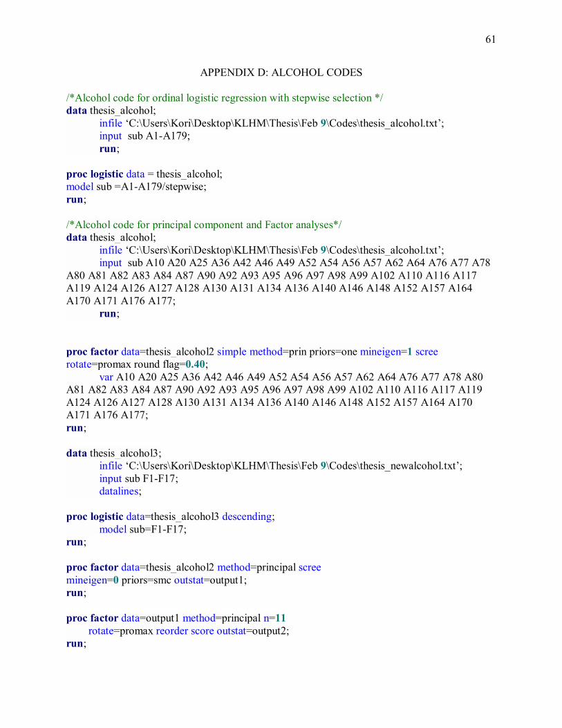
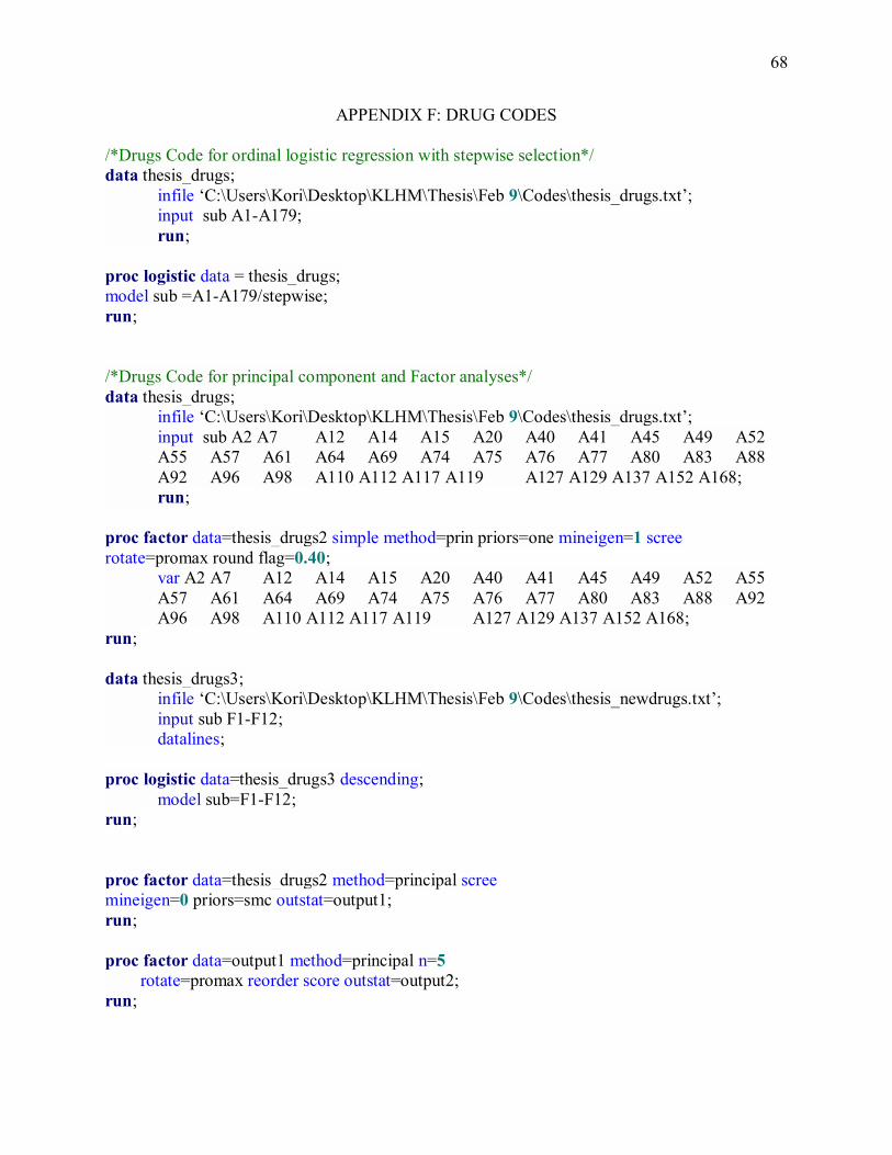
APPENDIX C : TOBACCO RESULTS 51 APPENDIX D : ALCOHOL CODES 61 APPENDIX E: ALCOHOL RESULTS 62 APPENDIX F : DRUG CODES 68 APPENDIX G : DRUG RESULTS 69
Page 9
vii
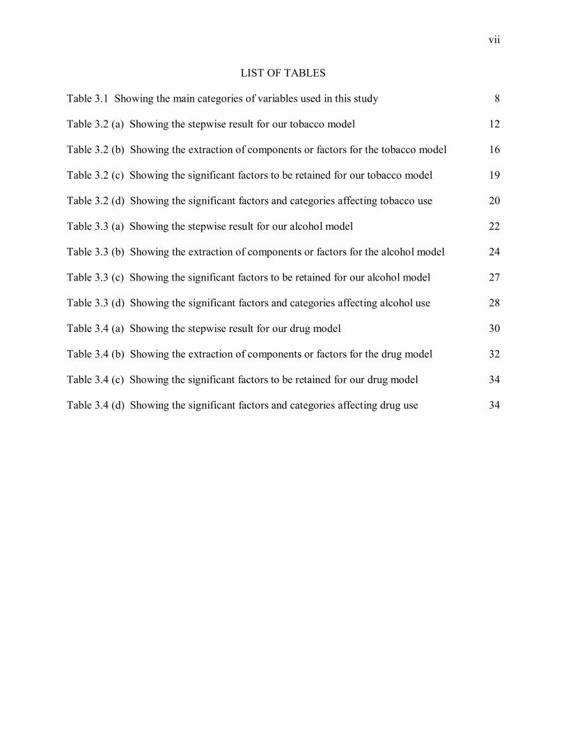
LIST OF TABLES
Table 3.1 Showing the main categories of variables used in this study 8 Table 3.2 (a) Showing the stepwise result for our tobacco model 12 Table 3.2 (b) Showing the extraction of components or factors for the tobacco model 16 Table 3.2 (c) Showing the significant factors to be retained for our tobacco model 19 Table 3.2 (d) Showing the significant factors and categories affecting tobacco use 20 Table 3.3 (a) Showing the stepwise result for our alcohol model 22 Table 3.3 (b) Showing the extraction of components or factors for the alcohol model 24 Table 3.3 (c) Showing the significant factors to be retained for our alcohol model 27 Table 3.3 (d) Showing the significant factors and categories affecting alcohol use 28 Table 3.4 (a) Showing the stepwise result for our drug model 30 Table 3.4 (b) Showing the extraction of components or factors for the drug model 32 Table 3.4 (c) Showing the significant factors to be retained for our drug model 34 Table 3.4 (d) Showing the significant factors and categories affecting drug use 34
Page 10
viii
LIST OF FIGURES
Figure 2.6 Showing the steps taken to fit our model 6 Figure 3.1 (a) Showing tobacco use by gender 9 Figure 3.1 (b) Showing alcohol use by gender 10 Figure 3.1 (c) Showing drug use by gender 10 Figure 3.2 Showing the scree plot of eigenvalues for our tobacco model 18 Figure 3.3 Showing the scree plot of eigenvalues for our alcohol model 26 Figure 3.4 Showing the scree plot of eigenvalues for our drug model 33
Page 11
1
CHAPTER 1
INTRODUCTION
Research has shown that children who abuse substances perform poorly in schools. They
use these substances as a means of acceptance or to gain attention. In this study, we want to
determine the significant factors that affect the use or abuse of substances in school aged
children and what can be done to prevent or reduce their effect.
In undertaking this study, information was obtained from the health behavior in school
aged children (HBSC) article from the Inter-University Consortium for Political and Social
Research website. Since our response variables are considered to be data with nominal levels
(qualitative measurements), we implement the logistic regression model. The purpose of this
study is to obtain a greater understanding of the health behavior and conduct of children and also
devise ways that may edify and influence their health behavior or practice.
The study (US Department of Health and Human Services, 1996) involved here is known
as Health Behavior in School-Aged Children (HBSC) and is an international survey of children
in as many as 30 countries worldwide. The data used here is from the United States survey
conducted during the 2001-2002 school year. Data on a number of health behaviors and factors
which determine them was collected. The response variables in this model are various types of
substances such as tobacco, alcohol and drugs including marijuana, inhalants and other
substances. The independent variables include, but are not limited to, eating habits, body image,
health problems, family make up, personal injuries, aggressive behavior and the school�s policy
on violence and substance abuse. There were a total of fourteen thousand eight hundred and
seventeen (14,817) students from three hundred and forty (340) participating schools in the
United States from grades 6 through 10 for the 2001 to 2002 academic year. Missing cases were
Page 12
2
identified for some significant variables and were not included as a result. There were also
variables (for example, age) with imputed values which were reclassified using the average of
the values depending on the data range.
To perform our analysis on this data, we implemented the logistic regression model
which is considered to be an important tool used to analyze the relationship between several
explanatory variables and the qualitative response variables. This method facilitates the
determination of variables related to substance abuse and also to estimate the magnitude of the
overall effect of the explanatory variables on the outcome of our study.
If we suppose that there is a single quantitative explanatory variable (X), for a binary
response variable (Y), we note that π(x) denotes the �success� probability at value x. The
probability is the parameter for the binomial distribution (Agresti, 2007). The logistic regression
model has linear form for the logit of this probability as follows:
logit[π(x)] = log[π(x)/1- π(x)] = α + βx
where α and β are the regression parameters estimated by the maximum likelihood method
(Agresti, 1996).
Our purpose is to determine which of the categories of variables in the survey contribute
significantly to the use or abuse of substances in school aged children and suggest what can be
done to prevent or reduce their effect. In the upcoming chapters we will focus, in depth, on the
methodology that was used. In this case, logistic regression analysis was implemented to
determine the significant contributory factors influencing the use and abuse of substances,
particularly tobacco, alcohol and drugs on school aged children. In chapter 3, we will discuss the
results of our findings and, finally, chapter 4 discusses our conclusion from our findings.
Page 13
3
CHAPTER 2
METHODOLOGY
2.1 Introduction
Our data contains several variables obtained from the HBSC survey. In order to
appropriately consider all factors that, through extensive research performed, are believed to
affect the level of substance abuse, the following was done. In our initial selection of variables,
we looked for factors that clearly demonstrated risk or protective properties and also for
variables significant for univariate regression (with a p-value <0.25). Risk factors are those
factors believed to have a negative impact on the likelihood of substance abuse while protective
factors are those factors that, when in place, are believed to significantly reduce the likelihood of
substance abuse. After these factors were identified for our model, the logistic regression
procedure was used in combination with the stepwise selection method. This enabled us to select
those significant variables which impact substance abuse, while at the same time removing those
variables which have a lesser impact. The principal component analysis, along with factor
analysis was then utilized, which allowed us to highlight patterns in the data and identify any
similarities and differences. This was done to determine the combination of variables which have
a significant impact on substance abuse.
2.2 Ordinal Regression Model
The application of the ordinal regression model is dependent, in large part, on the
measurement scale of the variables and the underlined assumptions. If the measurement scale of
our response variables is ordered (for example, every day, more than once a week, once a week,
once a month and rarely or never), the ordinal regression model is a preferred modeling tool
Page 14
4
which does not assume normality or constant variance, but requires the assumption of parallel
lines across all levels of the outcome.
The ordinal regression model may take the following form if the logit link is applied:
log {[ P(Y ≤ yj | X)] / [P(Y >yj | X)]}= αj + β1Xj1 + β2Xj2 +� + βpXjp, j = 1, 2, �, k and, where j
is the index of categories of response variables. For multiple explanatory variables in the model,
we would use β1Xj1 + β2Xj2 +� + βpXjp (Bender, 2000).
2.3 Logistic Regression Model
The logistic regression model or the logit model as it is often referred to, is a special case
of a generalized linear model and analyzes models where the outcome is a nominal variable.
Analysis for the logistic regression model assumes the outcome variable is a categorical variable.
It is common practice to assume that the outcome variable, denoted as Y, is a dichotomous
variable having either a success or failure as the outcome.
For logistic regression analysis, the model parameter estimates (α, β1, β2,�,βp) should be
obtained and it should be determined how well the model fits the data (Agresti, 2007). In this
study, the potential explanatory variables were examined to determine whether or not they are
significant enough to be used in our models. The complete model contained all the explanatory
variables and interactions believed to influence the level of substance abuse. From that initial
stage, we performed regression analysis with the stepwise selection procedure to select our
significant variables. Then, factor analysis was used to determine the significant combination of
Page 15
5
factors in our model. For our purposes, significant combinations of factors have large
eigenvalues greater than 1.
2.4 Model Assumptions
For our ordinal regression model to hold, we need to ensure that the assumption of
parallel lines of all levels of the categorical data is satisfied since the model does not assume
normality and constant variance (Bender and Benner, 2000).
Logistic regression does not assume a linear relationship between the dependent and
independent variables, the dependent variables do not need to be normally distributed, there is no
homogeneity of variance assumption, in other words, the variances do not have to be the same
within categories, normally distributed error terms are not assumed and the independent
variables do not have to be interval or unbounded (Wright, 1995).
2.5 Fitting the Data
Since we fit a logistic regression model, we assume that the relationships between the
independent variables and the logits are equal for all logits. The regression coefficients are the
coefficients α, β1, β2,�,βp of the equation:
Logit[π(x)] = α + β1X1 + β2X2 +� + βpXp
The results would therefore be a set of parallel lines for each category of the outcome
variables. This assumption can be checked by allowing the coefficients to vary, estimating them
and determining if they are all equal. So our maximum likelihood parameter estimates,
diagnostic and goodness of fit statistics, residuals and odds ratios were obtained from the final
fitted logistic regression model.
Page 16
6
2.6 Analyzing the Data
Here, the logistic regression model was used to select the significant variables that are
believed to contribute to substance abuse in children. Factor analysis was also used to identify
the combination of variables that have a significant impact on the abuse of substances. After
these variables and combination of variables were identified, the risk and protective factors were
revisited to determine where they fit and how best to relate it to the level of substance abuse.
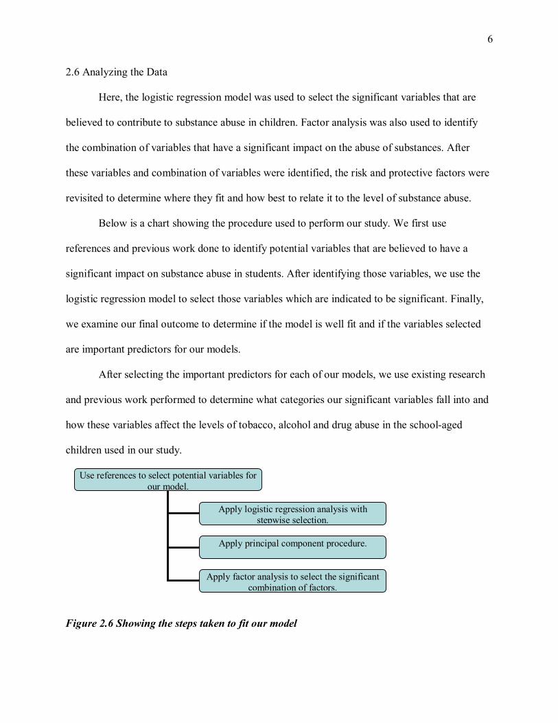
Below is a chart showing the procedure used to perform our study. We first use
references and previous work done to identify potential variables that are believed to have a
significant impact on substance abuse in students. After identifying those variables, we use the
logistic regression model to select those variables which are indicated to be significant. Finally,
we examine our final outcome to determine if the model is well fit and if the variables selected
are important predictors for our models.
After selecting the important predictors for each of our models, we use existing research
and previous work performed to determine what categories our significant variables fall into and
how these variables affect the levels of tobacco, alcohol and drug abuse in the school-aged
children used in our study.
Figure 2.6 Showing the steps taken to fit our model
Use references to select potential variables for our model.
Apply logistic regression analysis with stepwise selection.
Apply principal component procedure.
Apply factor analysis to select the significant combination of factors.
Page 17
7
CHAPTER 3
RESULTS
3.1 Overview
There are a number of factors which can contribute to the abuse of substances. Two main
types of factors that will be focused on in this study are risk and protective factors. From
research conducted through the National Institute on Drug Abuse (NIDA), risk factors are those
factors that increase the risk or likelihood of an individual being affected by the misuse of
substances. On the other hand, protective factors are those factors which reduce the likelihood of
substance abuse.
Risk factors can influence substance abuse in many different ways. The more risks a
child is exposed to, the greater the likelihood of substance abuse. Such risk factors include
aggressive behavior, lack of parental supervision, poverty and drug availability. Protective
factors help in reducing the likelihood of substance abuse and include such factors as parental
monitoring, academic competence and neighborhood or community attachment.
These factors were therefore taken into consideration when selecting variables for our
models. After these factors were initially selected the logistic regression analysis with stepwise
selection was performed to determine which variables significantly influence the abuse of our
substances. The principal component analysis was performed to select significant factors for our
model, and then we applied the logistic procedure again to determine which of those factors
should be retained for further analysis. Finally, factor analysis was then used to determine the
combination of variables that are considered to be significant. The substances that we will
concentrate on here are Tobacco, Alcohol and Drugs and the main categories of predictors are
outlined in the following table:
Page 18
8
Table 3.1 Showing the main categories of variables used in this study
Variables Meaning
Involved in clubs Whether the student was involved in any organizations or clubs.
Living arrangements Determining who the student lives with
Drink alcohol Whether the student drinks alcohol or has ever been drunk
Dieting/Weight control
behavior
Determining if the student uses pills or other methods to control
their weight
Close female friends Determining if the student has close female relationships
Carry weapons Whether the student has carried weapons in the last 30 days
Family vacation If the student goes on family vacations
Tried smoking Determining if the student ever tried smoking
Frequency of drinking Determining how often the student consumes any alcoholic
beverage
Marijuana/inhalant use If the student ever used marijuana or inhalants
Bullied others/been bullied Whether the student is guilty of bullying others or being bullied
Safe/comfortable
neighborhood
Determining if the student resides in a safe friendly
environment/community
Made fun of If the student has been made fun of because of race or religion.
Been in a Fight If they have ever been in a physical confrontation or fight.
Relationship with Family Determining their relationship with family members.
Feeling towards Education How they feel about school and their academic progress.
School�s tobacco policy How the school feels about tobacco use
Adult Responsible Determining who is responsible for the student
School�s violence
protection program
What measures the school implements to protect its students
Life rating How satisfied the student is about his/her life
Substance use Whether the student uses any of the substances and the frequency
of use
Parent�s Education Highest level of education achieved by Parents
Page 19
9
Watching TV Time spent watching the television
Doing homework Time spent doing homework
Computer/Internet use Time spent on the computer
Physical Activity How physically active is the student
Eating habits/nutrition If the student has well balanced meals
Self image How the student feels about their body/image
Parent�s occupation What kind of job/career do their parents have
As can be seen through our analysis, our substances are related in some ways. They have
similar risk and protective factors which seem to influence the level of abuse a student
undergoes. It should be pointed out though that every child is different so different factors can
affect individuals at different stages of development but if it is suspected that a substance is
being abused, the child should be monitored closely and carefully. The following graphs detail
the level of use of the three substances in our model by both males and females in the survey. It
should be noted that there were more females than males in the overall study so their levels may
be greater than that of the males. It should also be pointed out that peer relationships have been a
significant factor for all three of our models which indicates that a student�s relationship with
people his or her own age has a substantial impact on the level of substance abuse exhibited.
Chart showing tobacco use by gender
Yes Yes
NoNo
0
1000
2000
3000
4000
5000
6000
Boys Girls
Gender
Toba
cco
use
YesNo
Figure 3.1 (a) Showing tobacco use by gender
Page 20
10
Figure 3.1 (a) compares the tobacco use between males and females. Of the 6,412 boys,
1908 indicated using tobacco while 4,504 did not. 2,034 girls indicated using tobacco while
4,955 did not, out of the total of 6,988.
Chart showing alcohol use by gender
YesYes
NoNo
0500
10001500200025003000350040004500
Boys Girls
Gender
Alco
hol u
se
YesNo
Figure 3.1 (b) Showing alcohol use by gender
Figure 3.1(b) also compares the use of alcohol by gender. Of the 6,298 boys, 2,603 used
alcohol and 3,695 did not and of the 6,864 girls, 2,859 used alcohol and 4,005 did not.
Chart showing drug use by gender
YesYes
NoNo
0200400600800
10001200140016001800
Boys Girls
Gender
Drug
use Yes
No
Figure 3.1 (c) Showing drug use by gender
Page 21
11
Similarly, Figure 3.1(c) compares drug use between males and females in this study. Of the
2,225 boys, 775 used drugs while 1,479 did not and of the 2,514 girls, 907 used drugs and 1,607
did not.
3.2 Tobacco Results
The probit and logit models are techniques used to analyze the relationship between
independent variables and a binary dependent variable. The main reason for using logits in this
study is that when a linear model using probabilities does not fit the data properly, a linear model
using logits does (DeMaris, 1992). For the tobacco model, the dependent variable is whether the
student has ever smoked tobacco or not, so we are interested in the factors that influence whether
or not a student uses tobacco. The outcome is binary (yes or no) and the predictor variables are
those selected based on their risk or protective factors. From the output obtained using the logit
procedure in SAS, we see that the output describes and tests the overall fit of the model. The
likelihood ratio chi-square of 8456.8384 with a p-value of <0.0001 tells us that the effect of the
factors is deemed significant for our model.
Our analysis has allowed us to determine the significant contributory factors responsible
for the use and abuse of tobacco in school aged children using the logistic regression method and
the stepwise selection procedure. In stepwise selection, an attempt is made to remove any
insignificant variables from the model before adding a significant variable to the model. Each
addition or subtraction of a variable to or from the model is listed as a separate step in the results
and at each step a new model is fitted. The following table provides the result of our logistic
regression procedure with stepwise selection method to determine the significant variables for
our tobacco model.
Page 22
12
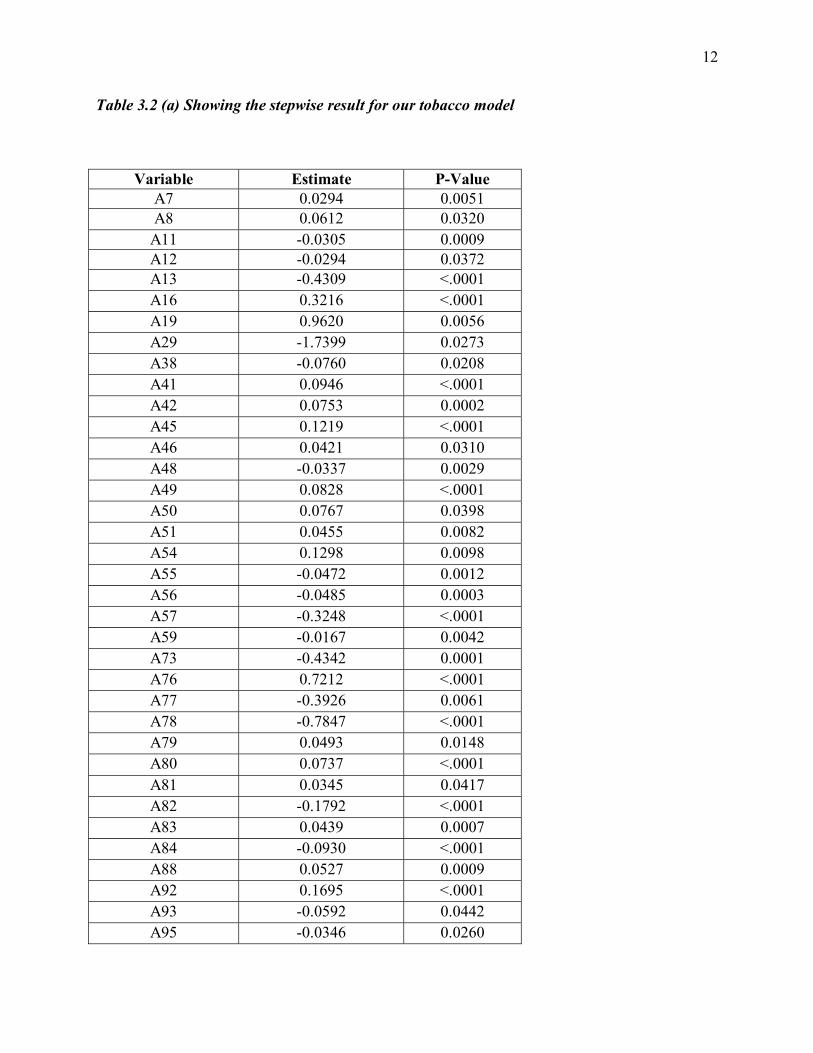
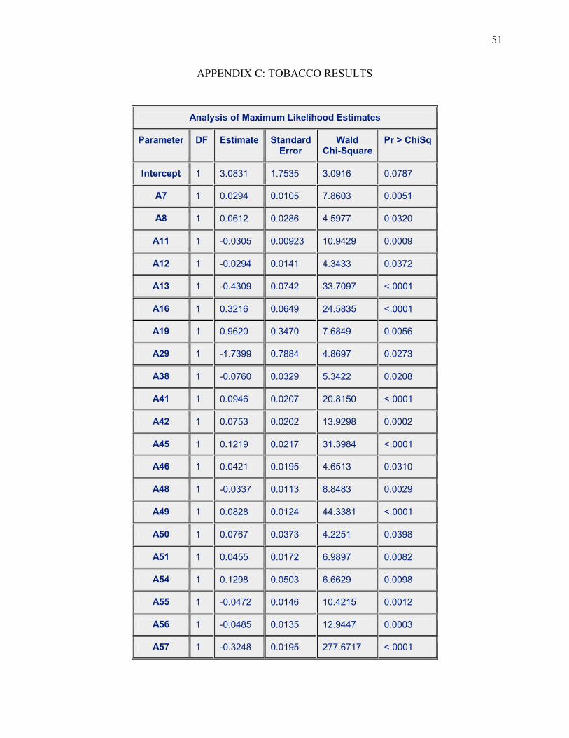
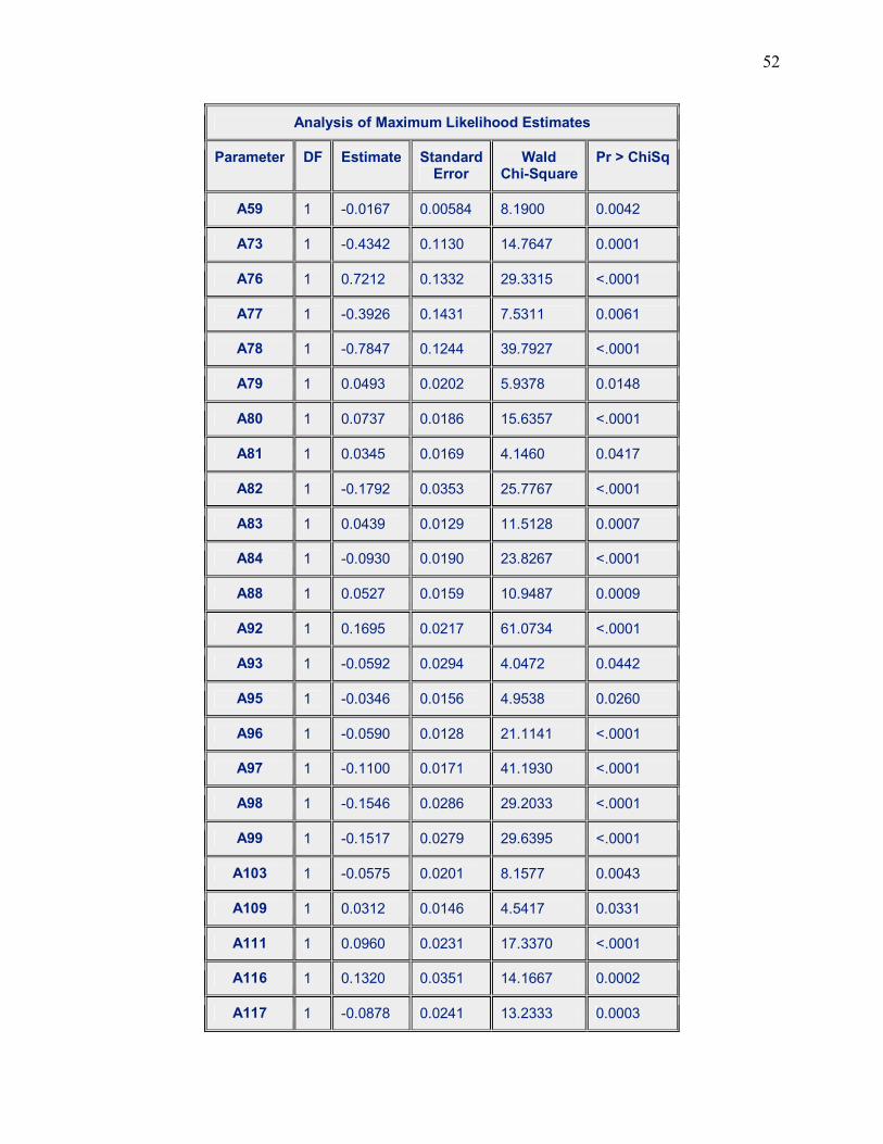
Table 3.2 (a) Showing the stepwise result for our tobacco model
Variable Estimate P-Value A7 0.0294 0.0051 A8 0.0612 0.0320
A11 -0.0305 0.0009 A12 -0.0294 0.0372 A13 -0.4309 <.0001 A16 0.3216 <.0001 A19 0.9620 0.0056 A29 -1.7399 0.0273 A38 -0.0760 0.0208 A41 0.0946 <.0001 A42 0.0753 0.0002 A45 0.1219 <.0001 A46 0.0421 0.0310 A48 -0.0337 0.0029 A49 0.0828 <.0001 A50 0.0767 0.0398 A51 0.0455 0.0082 A54 0.1298 0.0098 A55 -0.0472 0.0012 A56 -0.0485 0.0003 A57 -0.3248 <.0001 A59 -0.0167 0.0042 A73 -0.4342 0.0001 A76 0.7212 <.0001 A77 -0.3926 0.0061 A78 -0.7847 <.0001 A79 0.0493 0.0148 A80 0.0737 <.0001 A81 0.0345 0.0417 A82 -0.1792 <.0001 A83 0.0439 0.0007 A84 -0.0930 <.0001 A88 0.0527 0.0009 A92 0.1695 <.0001 A93 -0.0592 0.0442 A95 -0.0346 0.0260
Page 23
13
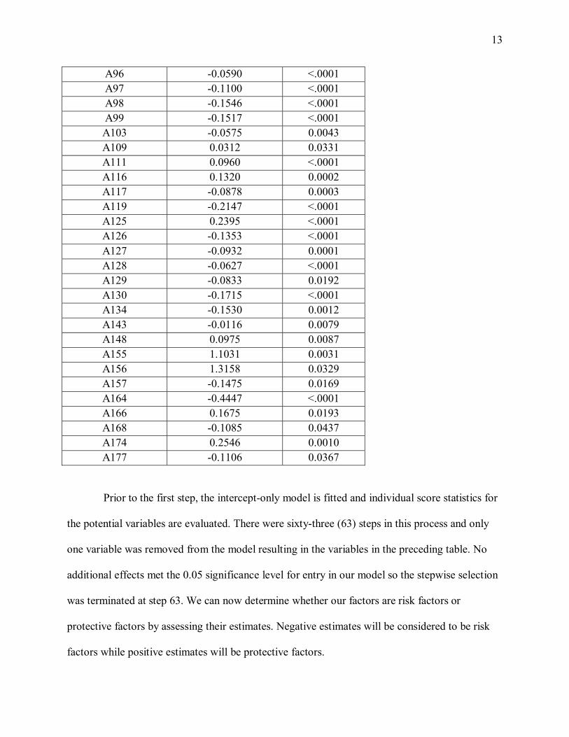
A96 -0.0590 <.0001 A97 -0.1100 <.0001 A98 -0.1546 <.0001 A99 -0.1517 <.0001 A103 -0.0575 0.0043 A109 0.0312 0.0331 A111 0.0960 <.0001 A116 0.1320 0.0002 A117 -0.0878 0.0003 A119 -0.2147 <.0001 A125 0.2395 <.0001 A126 -0.1353 <.0001 A127 -0.0932 0.0001 A128 -0.0627 <.0001 A129 -0.0833 0.0192 A130 -0.1715 <.0001 A134 -0.1530 0.0012 A143 -0.0116 0.0079 A148 0.0975 0.0087 A155 1.1031 0.0031 A156 1.3158 0.0329 A157 -0.1475 0.0169 A164 -0.4447 <.0001 A166 0.1675 0.0193 A168 -0.1085 0.0437 A174 0.2546 0.0010 A177 -0.1106 0.0367
Prior to the first step, the intercept-only model is fitted and individual score statistics for
the potential variables are evaluated. There were sixty-three (63) steps in this process and only
one variable was removed from the model resulting in the variables in the preceding table. No
additional effects met the 0.05 significance level for entry in our model so the stepwise selection
was terminated at step 63. We can now determine whether our factors are risk factors or
protective factors by assessing their estimates. Negative estimates will be considered to be risk
factors while positive estimates will be protective factors.
Page 24
14
As can be seen from the previous table, the variables have p-values less than 0.05 which
indicates their significance. The variables that can have risk properties in this model are lack of
organization involvement, lack of parental supervision, signs of aggressive behavior, weight
control behavior and having a foster home are risk factors that are of concern. Previous studies
have determined that a lack of involvement in community or social based organizations can
result in a student being tempted to abuse substances. A lack of physical activity or involvement
in sports can result in students being idle too often and filling their time experimenting with
harmful substances. This is also true if they do not have a stable home or family life. If their
parents are not in the main home to look out for them, or if they are constantly transported from
one foster home to the next, they are not accustomed to a stable environment so they abuse drugs
to fill the void. Carrying weapons and calling other students names also exhibits certain
aggressive behavior which is a key sign of substance abuse especially if it is out of character for
the student. This allows them to also be susceptible to other abuses. Also, a poor life rating or
lack of close friends may allow feelings of depression and loneliness to set in and, in order to fill
that void, the student turns to smoking. A lack of parental supervision and a lack of
organizational attachment are important risk factors associated with tobacco abuse. If the school
community does not have adequate measures in place to prevent gang violence, then weaker
students may become victims and may turn to substances in order to cope. On the other hand, the
protective factors identified here are professional weight control behavior where the student can
be sufficiently monitored; whether the student is physically active which reduces the likelihood
of substance abuse if he or she participates in extracurricular activities. For students who have an
affluent family life and positive family relationships, that is, they are not in foster care or going
from home to home and their family is well off which allows them the opportunity to take
Page 25
15
vacations, this will lead to positive feelings about their lives and this is a protective factor against
tobacco use. If they spend sufficient time with family, they will feel more comfortable
expressing their problems and seeking help if necessary.
Due to the large number of significant variables in our model, we will not be able to fit
the model with interaction variables; instead, we will now consider the principal component
analysis to determine if our predictor variables are sufficient for this model. A statistical
approach analyzing the inter-relationships among a significant number of variables and
explaining these variables in terms of the underlying dimensions is known as factor analysis.
There are two main types; Principal component analysis, which examines the total variance
among the variables so the solution generated will include as many factors as there are variables;
and the Common factor analysis which uses an estimate of common variance among the original
variables resulting in the factor solution. In this instance, the number of factors will be less than
the number of original variables so selecting the factors to retain for further analysis is more
problematic using common factor analysis (Rummel, 1984).
There are four main steps in conducting factor analysis. First, we collect the data and
generate the correlation matrix. We then extract the initial factor solution; thirdly, interpret our
output and finally, we construct scales or factor scores to use in further analysis. The output of
the factor analysis in the table below details the number of components or factors to be retained
for further analysis. In determining the number of factors, it is common practice or a general rule
of thumb to select those factors with eigenvalues greater than 1.
The following table details the result from our application of the principal component
procedure using the SAS program. This table details the eigenvalues, the proportion of variance
in the data for each factor as well as the cumulative variance in the data as the factor solution.
Page 26
16
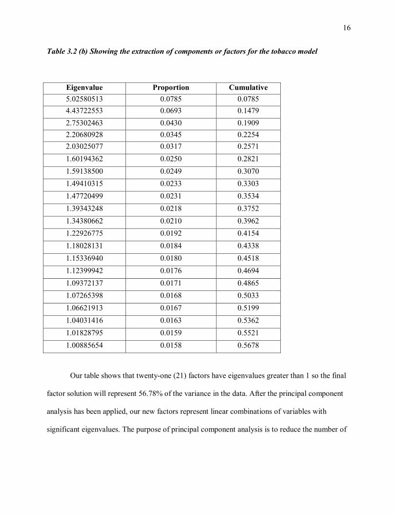
Table 3.2 (b) Showing the extraction of components or factors for the tobacco model
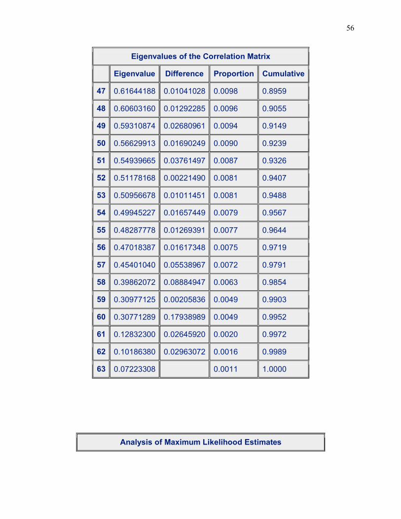
Eigenvalue Proportion Cumulative 5.02580513 0.0785 0.0785 4.43722553 0.0693 0.1479 2.75302463 0.0430 0.1909 2.20680928 0.0345 0.2254 2.03025077 0.0317 0.2571 1.60194362 0.0250 0.2821 1.59138500 0.0249 0.3070 1.49410315 0.0233 0.3303 1.47720499 0.0231 0.3534 1.39343248 0.0218 0.3752 1.34380662 0.0210 0.3962 1.22926775 0.0192 0.4154 1.18028131 0.0184 0.4338 1.15336940 0.0180 0.4518 1.12399942 0.0176 0.4694 1.09372137 0.0171 0.4865 1.07265398 0.0168 0.5033 1.06621913 0.0167 0.5199 1.04031416 0.0163 0.5362 1.01828795 0.0159 0.5521 1.00885654 0.0158 0.5678
Our table shows that twenty-one (21) factors have eigenvalues greater than 1 so the final
factor solution will represent 56.78% of the variance in the data. After the principal component
analysis has been applied, our new factors represent linear combinations of variables with
significant eigenvalues. The purpose of principal component analysis is to reduce the number of
Page 27
17
observed variables into a relatively smaller number of components. First, we examined the
eignevalue-one criterion where we selected those factors that have an eignevalue of at least one.
The rationale for this criterion is simple. Each observed variable contributes one unit of
variance to the total variance in the data set. Any component that displays an eigenvalue greater
than 1 is accounting for a greater amount of variance than had been contributed by one variable.
This component will therefore account for a significant amount of variance and is worth
retaining. Conversely, components with eigenvalues less than 1 account for less variance than
had been contributed by one variable. Since the purpose of the principal component analysis is to
reduce the number of observed variables into a smaller number of components, this will not be
achieved effectively if components that account for less variance than had been contributed by
individual variables are retained. To confirm our results of 21 factors, we apply the scree test of
eigenvalues.
The scree test is a plot of the eigenvalues associated with each component to determine if
there is a break between the components with relatively large eigenvalues and those with small
eigenvalues (Cattell, 1966). The scree plot graphs the eigenvalue against the component number.
We can see as we go further down the graph that the pattern smoothes out. This means that each
successive component is accounting for a smaller and smaller amount of the total variance. We
will continue to keep only those principal components whose eigenvalues are greater than one.
Components with an eignevalue less than one account for less variance than did the original
variable and so are of little use in our study. So the point of principal component analysis is to
redistribute the variance in the correlation matrix to redistribute the variance to the first
components extracted using the method of eigenvalue decomposition.
Page 28
18
Figure 3.2 Showing the scree plot of eigenvalues for our tobacco model
Scree Plot of Eigenvalues ‚ ‚ 5 ˆ ‚ ‚ 1 ‚ ‚ 2 ‚ ‚ 4 ˆ ‚ ‚ ‚ ‚ E ‚ i ‚ g 3 ˆ e ‚ n ‚ 3 v ‚ a ‚ l ‚ u ‚ 4 e 2 ˆ 5 s ‚ ‚ ‚ 67 ‚ 890 ‚ 12 ‚ 3456 1 ˆ 7 89012 345 ‚ 67 89012 34 ‚ 567 89012 34 ‚ 567 89012 3 ‚ 4567 8 ‚ 90 ‚ 12 3 0 ˆ ‚ ‚ Šƒƒƒƒƒˆƒƒƒƒƒˆƒƒƒƒƒˆƒƒƒƒƒˆƒƒƒƒƒˆƒƒƒƒƒˆƒƒƒƒƒˆƒƒƒƒƒˆƒƒƒƒƒˆƒƒƒƒƒˆƒƒƒƒƒˆƒƒƒƒƒˆƒƒƒƒƒˆƒƒƒƒƒˆƒƒƒƒƒƒ 0 5 10 15 20 25 30 35 40 45 50 55 60 65 Number
Page 29
19
Figure 3.2 shows the scree test for our tobacco model. It can be seen that we have twenty-
one components greater than 1 on our scree plot, which confirms our previous conclusion. We
will now use the logistic procedure to determine how many of our twenty-one factors identified
previously are significant. As can be seen in the following table, our logistic procedure has
allowed us to retain seven of our twenty-one factors as significant factors for our tobacco model.
Table 3.2 (c) Showing the significant factors to be retained for our tobacco model
Factor Estimate P-value F1 -0.5818 <.0001 F2 0.0933 <.0001 F3 0.1500 <.0001 F4 0.3823 <.0001 F5 -0.0679 <.0001 F6 0.0395 0.0299 F7 0.0744 <.0001
The result of our factor analysis has allowed us to draw conclusions about the significant
combination of factors or variables which have a significant impact on tobacco use among
school-aged children. In the tobacco model, we have seven significant factors. The combinations
of variables that are believed to be influential are outlined in Table 3.2 (d). For our final tobacco
model, we acquired the significant combination of variables that affect tobacco use among
school-aged children and we grouped them into categories based on existing work and prior
knowledge gained. Table 3.2 (d) breaks down our results for the tobacco model. It should be
noted that all our variables (63) from our logistic procedure with stepwise selection method are
Page 30
20
considered to be significant. However, in Table 3.2 (d), we outline the most significant
combinations of variables, based on their relatively high value, and their related categories.
Table 3.2 (d) Showing the significant factors and categories affecting tobacco use
Factors Values Combination of Variables Category 0.9412 Weight control behavior -
professional 0.9382 Feeling low 0.9267 Weight control behavior � other
1
0.9213 Weight control behavior - vomitting
Low self esteem
0.75091 Jokes at others 0.72659 Times in physical fight 0.67396 Jokes about them 0.57123 Who bullies you 0.48976 With whom fought 0.48356 Called others names 0.46875 Left out
2
0.40764 Going to bed/school hungry
Aggressive behavior
0.6595 Bad temper 0.6198 Talk to father 0.6013 Difficulty sleeping
3
0.5429 Health
Individual
0.6266 E-communication with friends 0.6212 Evening with friends 0.4455 Academic achievement
4
0.4067 Number of medically treated injuries from fights
Peer group
0.5611 Internet access at home 5 0.4307 Family vacations
Family affluence
0.6828 Lunch weekends 0.6393 Days without lunch 0.5013 Breakfast weekends 0.413 Lunch weekdays
6
0.4097 Days eat lunch at school
Health and Nutrition
0.5353 Physically active 0.5325 Homework, weekends
7
0.4857 Staff, no tobacco use on sch transport
School community
Page 31
21
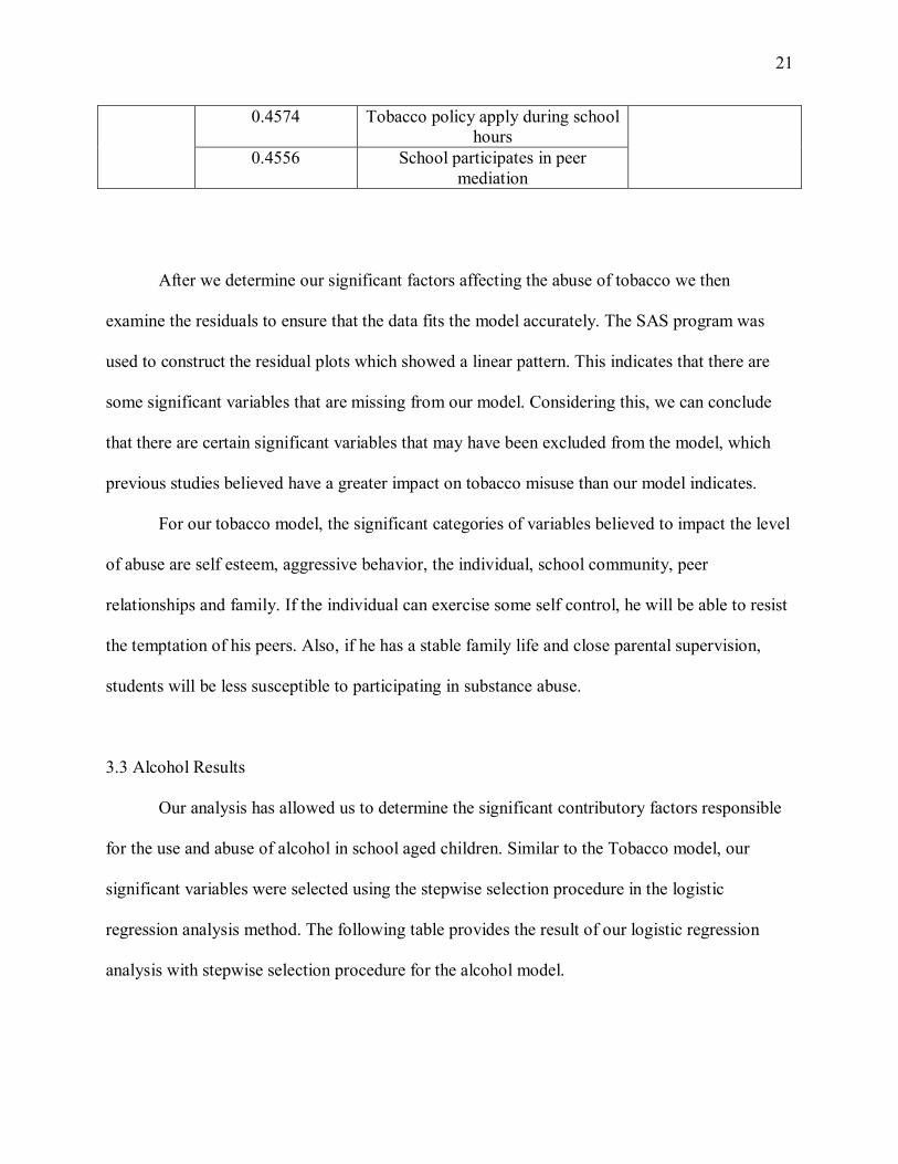
0.4574 Tobacco policy apply during school hours
0.4556 School participates in peer mediation
After we determine our significant factors affecting the abuse of tobacco we then
examine the residuals to ensure that the data fits the model accurately. The SAS program was
used to construct the residual plots which showed a linear pattern. This indicates that there are
some significant variables that are missing from our model. Considering this, we can conclude
that there are certain significant variables that may have been excluded from the model, which
previous studies believed have a greater impact on tobacco misuse than our model indicates.
For our tobacco model, the significant categories of variables believed to impact the level
of abuse are self esteem, aggressive behavior, the individual, school community, peer
relationships and family. If the individual can exercise some self control, he will be able to resist
the temptation of his peers. Also, if he has a stable family life and close parental supervision,
students will be less susceptible to participating in substance abuse.
3.3 Alcohol Results
Our analysis has allowed us to determine the significant contributory factors responsible
for the use and abuse of alcohol in school aged children. Similar to the Tobacco model, our
significant variables were selected using the stepwise selection procedure in the logistic
regression analysis method. The following table provides the result of our logistic regression
analysis with stepwise selection procedure for the alcohol model.
Page 32
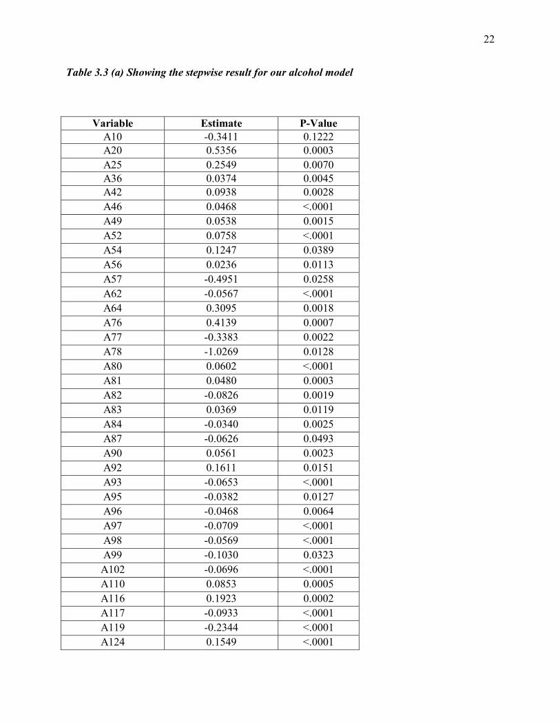
22
Table 3.3 (a) Showing the stepwise result for our alcohol model
Variable Estimate P-Value A10 -0.3411 0.1222 A20 0.5356 0.0003 A25 0.2549 0.0070 A36 0.0374 0.0045 A42 0.0938 0.0028 A46 0.0468 <.0001 A49 0.0538 0.0015 A52 0.0758 <.0001 A54 0.1247 0.0389 A56 0.0236 0.0113 A57 -0.4951 0.0258 A62 -0.0567 <.0001 A64 0.3095 0.0018 A76 0.4139 0.0007 A77 -0.3383 0.0022 A78 -1.0269 0.0128 A80 0.0602 <.0001 A81 0.0480 0.0003 A82 -0.0826 0.0019 A83 0.0369 0.0119 A84 -0.0340 0.0025 A87 -0.0626 0.0493 A90 0.0561 0.0023 A92 0.1611 0.0151 A93 -0.0653 <.0001 A95 -0.0382 0.0127 A96 -0.0468 0.0064 A97 -0.0709 <.0001 A98 -0.0569 <.0001 A99 -0.1030 0.0323 A102 -0.0696 <.0001 A110 0.0853 0.0005 A116 0.1923 0.0002 A117 -0.0933 <.0001 A119 -0.2344 <.0001 A124 0.1549 <.0001
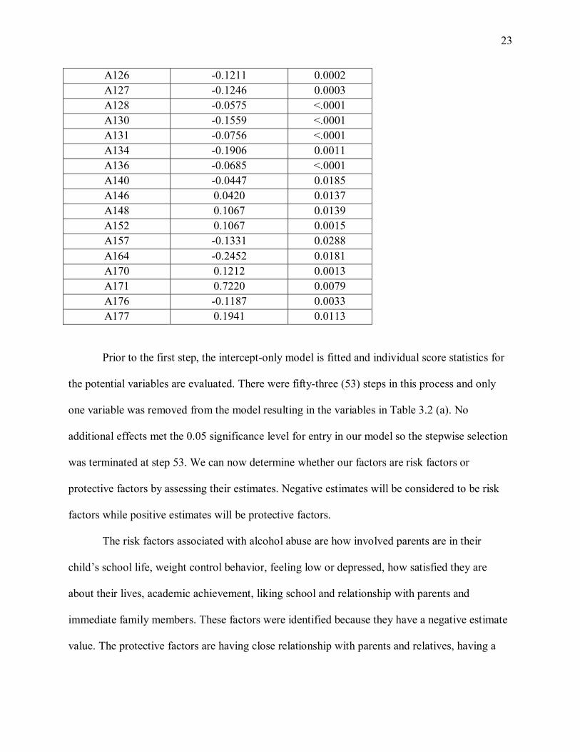
Page 33
23
A126 -0.1211 0.0002 A127 -0.1246 0.0003 A128 -0.0575 <.0001 A130 -0.1559 <.0001 A131 -0.0756 <.0001 A134 -0.1906 0.0011 A136 -0.0685 <.0001 A140 -0.0447 0.0185 A146 0.0420 0.0137 A148 0.1067 0.0139 A152 0.1067 0.0015 A157 -0.1331 0.0288 A164 -0.2452 0.0181 A170 0.1212 0.0013 A171 0.7220 0.0079 A176 -0.1187 0.0033 A177 0.1941 0.0113
Prior to the first step, the intercept-only model is fitted and individual score statistics for
the potential variables are evaluated. There were fifty-three (53) steps in this process and only
one variable was removed from the model resulting in the variables in Table 3.2 (a). No
additional effects met the 0.05 significance level for entry in our model so the stepwise selection
was terminated at step 53. We can now determine whether our factors are risk factors or
protective factors by assessing their estimates. Negative estimates will be considered to be risk
factors while positive estimates will be protective factors.
The risk factors associated with alcohol abuse are how involved parents are in their
child�s school life, weight control behavior, feeling low or depressed, how satisfied they are
about their lives, academic achievement, liking school and relationship with parents and
immediate family members. These factors were identified because they have a negative estimate
value. The protective factors are having close relationship with parents and relatives, having a
Page 34
24
stable home life with parents in the main home, having a close bond with their peers and being
physically active.
The risk factors are evident because if a child�s parent is not actively involved in their
school activities, they would not know what they are getting into so students may feel that they
can experiment with substances and not get caught. Students who feel low or depressed have a
tendency to use substances to make them feel better about themselves or at least to take their
minds off of their problems. Also, if the student is not doing well in school or not liking the
school environment, he or she may resort to abusing substances as a means of escaping. On the
other hand, it can be seen clearly that a feeling of acceptance is instrumental in the prevention of
alcohol abuse. If students have a sense of belonging and feel good enough and accepted, this
reduces the likelihood of them experimenting with alcohol. If they have a stable family life and
are surrounded by relatives who show care and concern for them, they will be less likely to have
a need to fill the void by abusing alcohol.
We will now proceed with principal component and factor analyses to determine the
significant combination of variables for our model. The following table details the result from
our application of the principal component procedure in SAS.
Table 3.3 (b) Showing the extraction of components or factors for the alcohol model
Eigenvalue Proportion Cumulative 4.58693518 0.0865 0.0865 3.52161327 0.0664 0.1530 2.50703957 0.0473 0.2003 2.06013610 0.0389 0.2392 1.64490179 0.0310 0.2702
Page 35
25
1.52459408 0.0288 0.2990 1.39318521 0.0263 0.3253 1.32893326 0.0251 0.3503 1.25133898 0.0236 0.3739 1.22451680 0.0231 0.3970 1.18688609 0.0224 0.4194 1.11148757 0.0210 0.4404 1.06550853 0.0201 0.4605 1.05381216 0.0199 0.4804 1.03130162 0.0195 0.4999 1.02611329 0.0194 0.5192 1.01490764 0.0191 0.5384
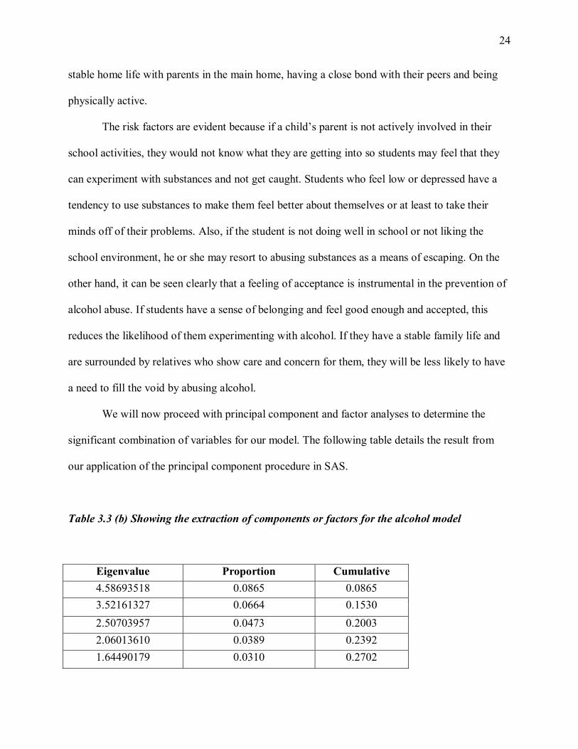
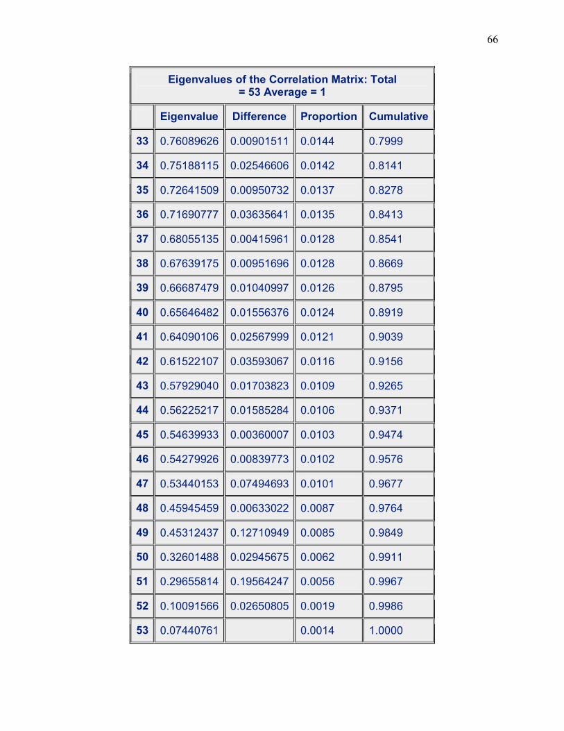
In this model, our results show that we have seventeen (17) eigenvalues greater than 1 so
the final factor solution will represent 53.84% of the variance in the data. To corroborate the
amount of factors to be retained, we perform further analysis using the scree test. This test will
help us to see graphically, all our significant factors with eigenvalues greater than one that we
wish to retain for our alcohol model.
Our graph shows that there are 17 factors with eigenvalues greater than 1 which confirms
our previous results. The factors below our cut-off point are not considered significant for further
analysis so they will not be retained. We will now refer to the logistic procedure to determine
how many of our significant factors we will retain for our model. As can be seen in the following
table, the logistic procedure has allowed us to retain eleven factors as significant for our drugs
model. As a result, further analysis will be performed on these eleven factors to determine how
they relate to substance abuse for our final alcohol model. Refer to Table 3.3 (c) which has the
results of our logistic analysis and Table 3.3 (d) which has the results of our analysis of our
significant factors retained for our model.
Page 36
26
Scree Plot of Eigenvalues ‚ ‚ 5 ˆ ‚ ‚ ‚ 1 ‚ ‚ ‚ 4 ˆ ‚ ‚ ‚ 2 ‚ E ‚ i ‚ g 3 ˆ e ‚ n ‚ v ‚ 3 a ‚ l ‚ u ‚ e 2 ˆ 4 s ‚ ‚ 5 ‚ 6 ‚ 7 ‚ 8 90 ‚ 1 2 1 ˆ 3 456 78 901 ‚ 23 456 78 901 ‚ 23 456 78 90 ‚ 1 23 456 7 ‚ 8 9 ‚ 01 ‚ 23 0 ˆ ‚ ‚ Šƒƒƒƒƒƒˆƒƒƒƒƒƒˆƒƒƒƒƒƒˆƒƒƒƒƒƒˆƒƒƒƒƒƒˆƒƒƒƒƒƒˆƒƒƒƒƒƒˆƒƒƒƒƒƒˆƒƒƒƒƒƒˆƒƒƒƒƒƒˆƒƒƒƒƒƒˆƒƒƒƒƒƒˆƒƒƒƒƒƒ 0 5 10 15 20 25 30 35 40 45 50 55 Number
Figure 3.3 Showing the scree plot of eigenvalues for our alcohol model
Page 37
27
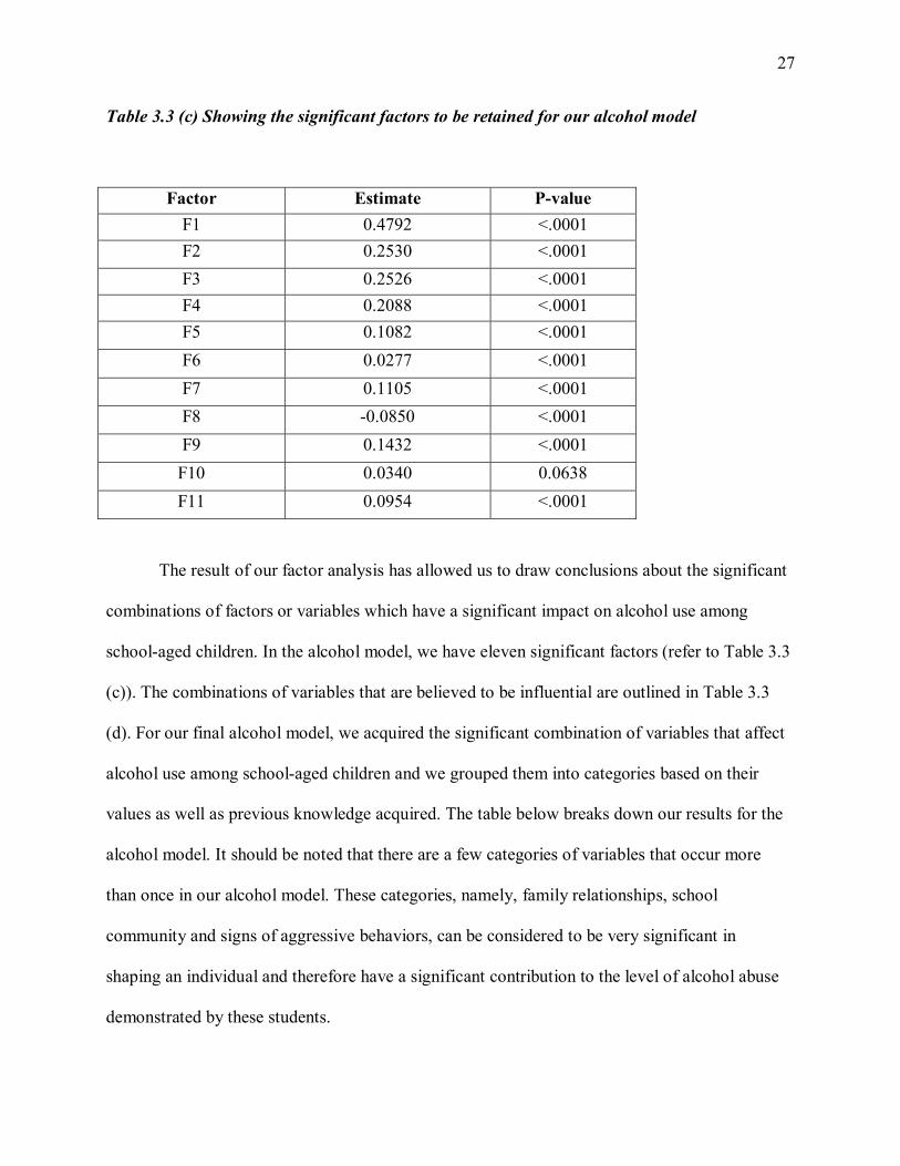
Table 3.3 (c) Showing the significant factors to be retained for our alcohol model
Factor Estimate P-value F1 0.4792 <.0001 F2 0.2530 <.0001 F3 0.2526 <.0001 F4 0.2088 <.0001 F5 0.1082 <.0001 F6 0.0277 <.0001 F7 0.1105 <.0001
F8 -0.0850 <.0001
F9 0.1432 <.0001
F10 0.0340 0.0638 F11 0.0954 <.0001
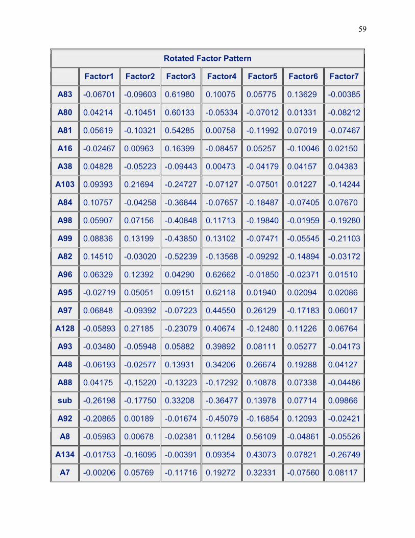
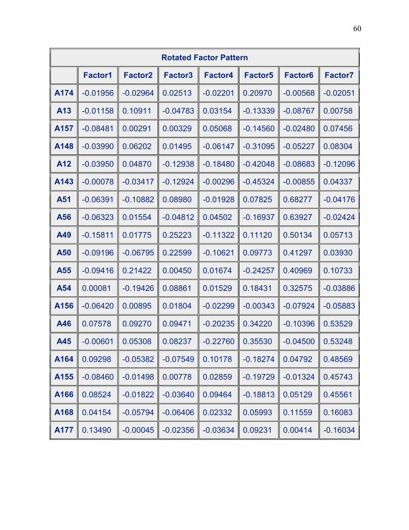
The result of our factor analysis has allowed us to draw conclusions about the significant
combinations of factors or variables which have a significant impact on alcohol use among
school-aged children. In the alcohol model, we have eleven significant factors (refer to Table 3.3
(c)). The combinations of variables that are believed to be influential are outlined in Table 3.3
(d). For our final alcohol model, we acquired the significant combination of variables that affect
alcohol use among school-aged children and we grouped them into categories based on their
values as well as previous knowledge acquired. The table below breaks down our results for the
alcohol model. It should be noted that there are a few categories of variables that occur more
than once in our alcohol model. These categories, namely, family relationships, school
community and signs of aggressive behaviors, can be considered to be very significant in
shaping an individual and therefore have a significant contribution to the level of alcohol abuse
demonstrated by these students.
Page 38
28
Table 3.3 (d) Showing the significant factors and categories affecting alcohol use
Factors Values Combination of Variables Category 0.9257 Weight control behavior-
other 0.9226 Feeling low 0.9144 Weight control behavior�
professional
1
0.5075 Weight control behavior� skip meals
Self/Body image
0.5287 Life satisfaction 0.4901 Student feels down, someone
helps 0.4816 People say hello 0.4702 Parents talk with teachers 0.4542 Talk to step dad
2
0.4221 Liking school
Community attachment
0.7767 Weapon type 0.7588 Family affluence 0.5631 With whom fought 0.4439 Go to school/bed hungry
3
0.4309 Number of medically treated injuries
Aggressive behavior
0.7093 Made fun of others � religion 0.77077 Times in physical fight 0.7032 Make jokes
4
0.6599 Who bullies you
Aggressive behavior
0.7558 Evening with friends 0.7402 E-communication with friends 0.4699 Academic achievement
5
0.4163 Close female friends
Peer relationships
0.7961 Step-dad in second home 6 0.6629 Talk to elder brother
Family relationships
0.5368 Talk to friend of same sex 7 0.5076 Close male friends
Peer relationships
0.6744 Written plan for in school violence
0.6378 After school transportation 0.5443 School requires visitors to
sign it
8
0.4234 School requires uniforms
School community
0.3462 Breakfast, weekends 9 0.3183 Days without lunch
Health/nutrition
Page 39
29
0.6154 Mom�s occupation 10 0.3302 Days without lunch
Family affluence
0.6356 School implement id badges 11 0.318 School policy � no tobacco in
school building
School community
After we determine our significant factors affecting the abuse of alcohol we then examine
the residuals to ensure that the data fits the model accurately. The SAS program was used to
construct the residual plots. Again, our residuals follow a linear pattern, so we conclude that our
model is not considered to be well fit and so, there are some variables that should be included in
our model but were not found to be significant.
We categorized our significant factors from our alcohol model into self or body image,
community attachment, aggressive behavior, peer and family relationships, health, nutrition and
the school community. Peer relationships can have a negative impact on a student as they want to
fit in and feel a sense of belonging so they often give in to the influences of their friends or the
people around them. Also, the individual has a role to play if he or she is strong-willed and
exercises self control then they can overcome the influences of their fellow students.
3.4 Drug Results
For our final model, our analysis has again allowed us to determine the significant
contributory factors responsible for the use and abuse of drugs in school aged children. The
probit and logits will be examined for the response variable and the factor or principal
component analysis will be computed for the explanatory variables. Here we are interested in the
factors that influence whether or not a student uses drugs. The outcome is binary (yes or no) and
the predictor variables are those selected based on their risk or protective factors in addition to
Page 40
30
the significance level (0.05). The following table provides the result of our stepwise regression
analysis for the drugs model.
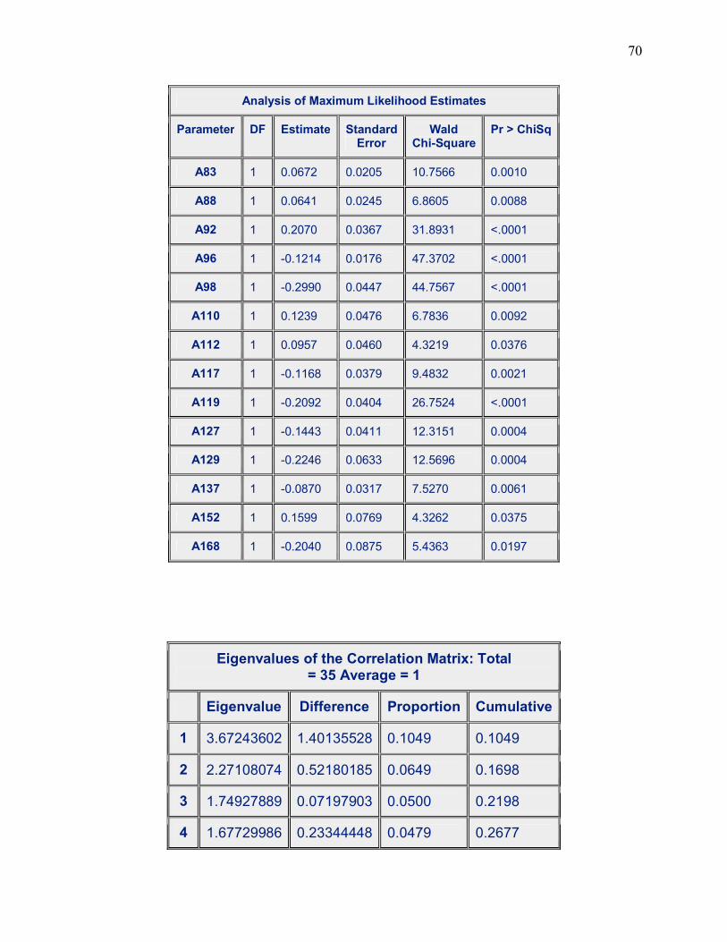
Table 3.4 (a) Showing the stepwise result for our drug model
Variable Estimate P-Value A2 0.0621 0.0123 A7 0.0399 0.0115
A12 -0.0668 0.0016 A14 -0.3900 <.0001 A15 0.5890 0.0032 A20 0.6747 0.0338 A40 -0.9471 0.0375 A41 0.1066 0.0004 A45 0.1421 <.0001 A49 0.0513 0.0060 A52 0.1254 0.0362 A55 -0.0791 0.0018 A57 -0.4305 <.0001 A61 0.1245 0.0086 A64 0.2320 0.0265 A69 -0.1931 0.0146 A74 -0.4093 0.0174 A75 0.4111 0.0072 A76 0.9189 <.0001 A77 -0.5566 0.0011 A80 0.0798 0.0044 A83 0.0672 0.0010 A88 0.0641 0.0088 A92 0.2070 <.0001 A96 -0.1214 <.0001 A98 -0.2990 <.0001 A110 0.1239 0.0092 A112 0.0957 0.0376 A117 -0.1168 0.0021 A119 -0.2092 <.0001 A127 -0.1443 0.0004
Page 41
31
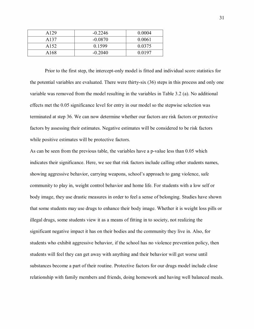
A129 -0.2246 0.0004 A137 -0.0870 0.0061 A152 0.1599 0.0375 A168 -0.2040 0.0197
Prior to the first step, the intercept-only model is fitted and individual score statistics for
the potential variables are evaluated. There were thirty-six (36) steps in this process and only one
variable was removed from the model resulting in the variables in Table 3.2 (a). No additional
effects met the 0.05 significance level for entry in our model so the stepwise selection was
terminated at step 36. We can now determine whether our factors are risk factors or protective
factors by assessing their estimates. Negative estimates will be considered to be risk factors
while positive estimates will be protective factors.
As can be seen from the previous table, the variables have a p-value less than 0.05 which
indicates their significance. Here, we see that risk factors include calling other students names,
showing aggressive behavior, carrying weapons, school�s approach to gang violence, safe
community to play in, weight control behavior and home life. For students with a low self or
body image, they use drastic measures in order to feel a sense of belonging. Studies have shown
that some students may use drugs to enhance their body image. Whether it is weight loss pills or
illegal drugs, some students view it as a means of fitting in to society, not realizing the
significant negative impact it has on their bodies and the community they live in. Also, for
students who exhibit aggressive behavior, if the school has no violence prevention policy, then
students will feel they can get away with anything and their behavior will get worse until
substances become a part of their routine. Protective factors for our drugs model include close
relationship with family members and friends, doing homework and having well balanced meals.
Page 42
32
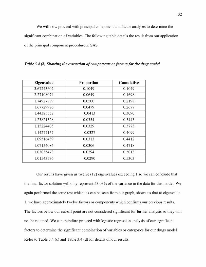
We will now proceed with principal component and factor analyses to determine the
significant combination of variables. The following table details the result from our application
of the principal component procedure in SAS.
Table 3.4 (b) Showing the extraction of components or factors for the drug model
Eigenvalue Proportion Cumulative 3.67243602 0.1049 0.1049 2.27108074 0.0649 0.1698 1.74927889 0.0500 0.2198 1.67729986 0.0479 0.2677 1.44385538 0.0413 0.3090 1.23821328 0.0354 0.3443 1.15224405 0.0329 0.3773 1.14277157 0.0327 0.4099 1.09516439 0.0313 0.4412 1.07154084 0.0306 0.4718 1.03035478 0.0294 0.5013 1.01543576 0.0290 0.5303
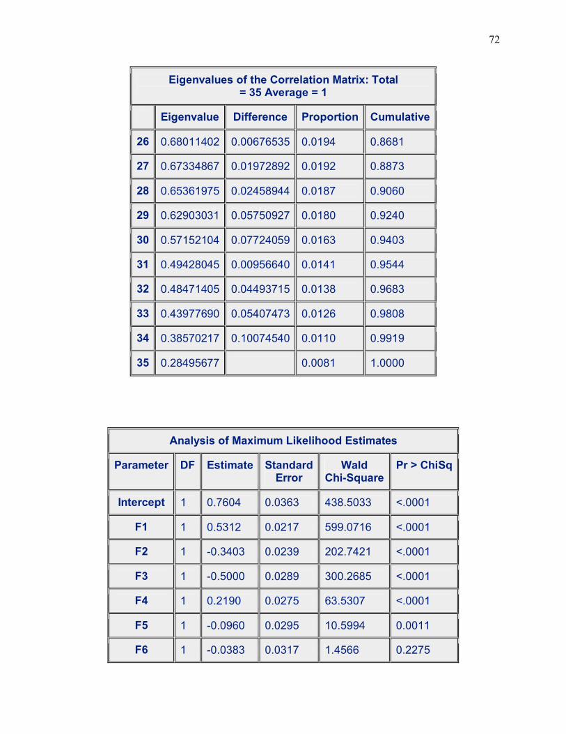
Our results have given us twelve (12) eigenvalues exceeding 1 so we can conclude that
the final factor solution will only represent 53.03% of the variance in the data for this model. We
again performed the scree test which, as can be seen from our graph, shows us that at eigenvalue
1, we have approximately twelve factors or components which confirms our previous results.
The factors below our cut-off point are not considered significant for further analysis so they will
not be retained. We can therefore proceed with logistic regression analysis of our significant
factors to determine the significant combination of variables or categories for our drugs model.
Refer to Table 3.4 (c) and Table 3.4 (d) for details on our results.
Page 43
33
Scree Plot of Eigenvalues ‚ ‚ ‚ ‚ ‚ ‚ 4 ˆ ‚ ‚ 1 ‚ ‚ ‚ ‚ 3 ˆ E ‚ i ‚ g ‚ e ‚ n ‚ 2 v ‚ a 2 ˆ l ‚ u ‚ 3 4 e ‚ s ‚ 5 ‚ 6 ‚ 7 8 9 0 1 ˆ 1 2 3 4 5 ‚ 6 7 8 9 0 1 2 ‚ 3 4 5 6 7 8 ‚ 9 0 ‚ 1 2 3 4 ‚ 5 ‚ 0 ˆ ‚ ‚ ‚ ‚ ‚ Šƒƒƒƒƒƒƒƒƒˆƒƒƒƒƒƒƒƒƒˆƒƒƒƒƒƒƒƒƒˆƒƒƒƒƒƒƒƒƒˆƒƒƒƒƒƒƒƒƒˆƒƒƒƒƒƒƒƒƒˆƒƒƒƒƒƒƒƒƒˆƒƒƒƒƒƒƒƒƒˆƒƒƒƒƒƒƒƒƒƒ 0 5 10 15 20 25 30 35 Number
Figure 3.4 Showing the scree plot of eigenvalues for our drug model
Page 44
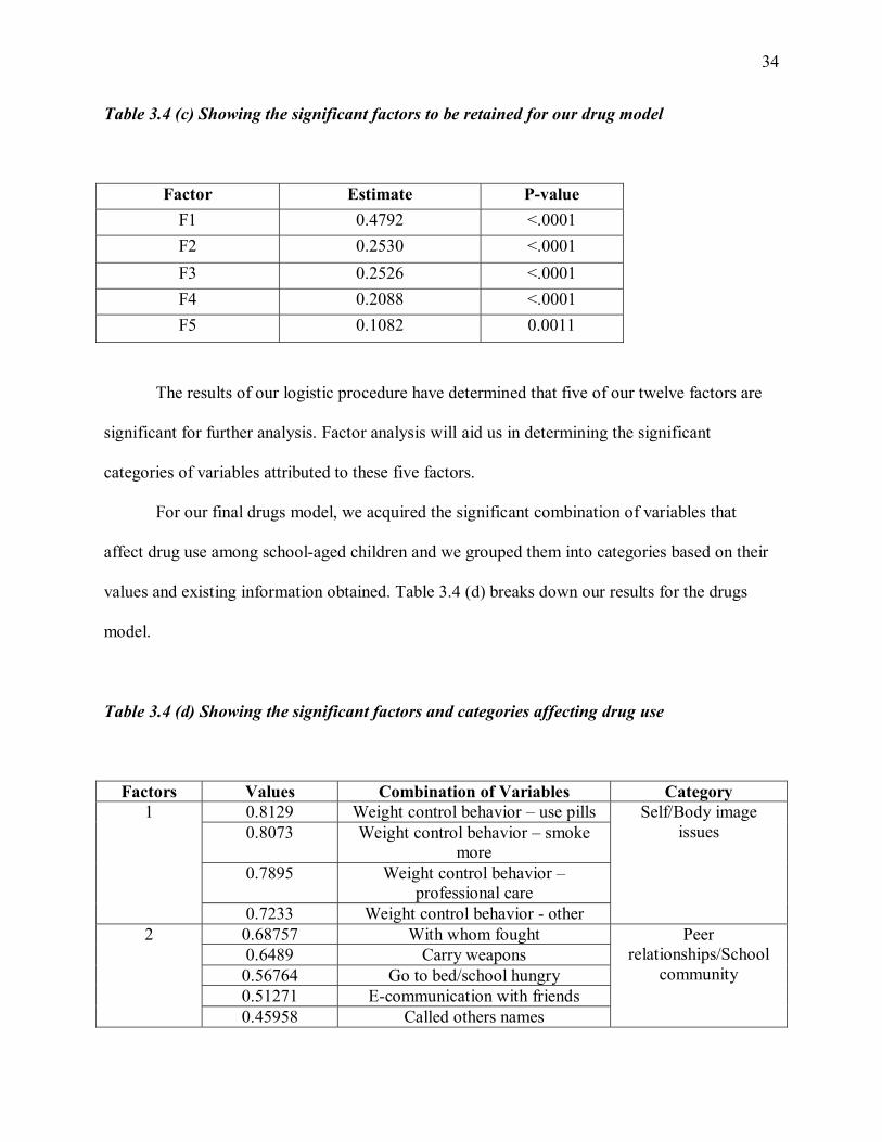
34
Table 3.4 (c) Showing the significant factors to be retained for our drug model
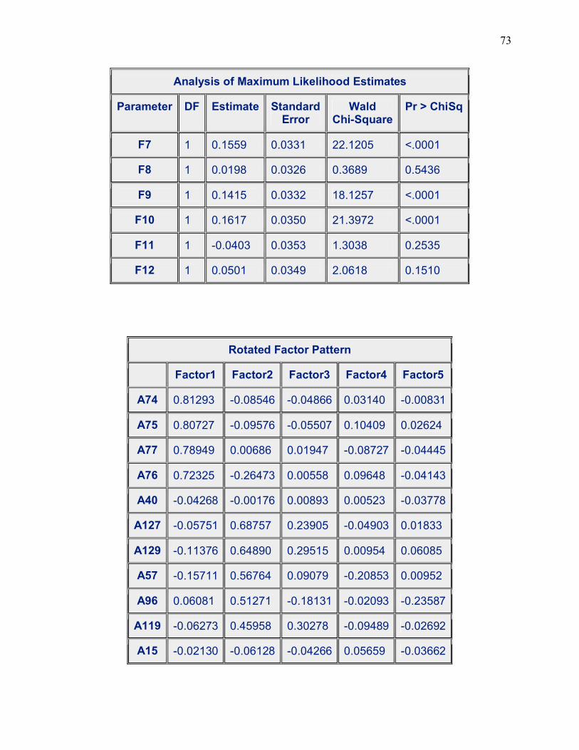
Factor Estimate P-value F1 0.4792 <.0001 F2 0.2530 <.0001 F3 0.2526 <.0001 F4 0.2088 <.0001 F5 0.1082 0.0011
The results of our logistic procedure have determined that five of our twelve factors are
significant for further analysis. Factor analysis will aid us in determining the significant
categories of variables attributed to these five factors.
For our final drugs model, we acquired the significant combination of variables that
affect drug use among school-aged children and we grouped them into categories based on their
values and existing information obtained. Table 3.4 (d) breaks down our results for the drugs
model.
Table 3.4 (d) Showing the significant factors and categories affecting drug use
Factors Values Combination of Variables Category 0.8129 Weight control behavior � use pills 0.8073 Weight control behavior � smoke
more 0.7895 Weight control behavior �
professional care
1
0.7233 Weight control behavior - other
Self/Body image issues
0.68757 With whom fought 0.6489 Carry weapons 0.56764 Go to bed/school hungry 0.51271 E-communication with friends
2
0.45958 Called others names
Peer relationships/School
community
Page 45
35
0.7487 Been hit, kicked or pushed 0.7247 Who usually bullies you
3
0.6633 Been called names
Aggressive behavior
0.57722 Difficulty sleeping 0.56128 Talk to father
4
0.43941 Breakfast, weekends
Individual
0.5834 Weight control behavior� skip meals0.5373 Mom in main home
5
0.4378 Weight control behavior- eat less
Self/Body image issues
Here, we notice that our drugs model has five significant factors. The categories for these
factors are body image, peer relationships, aggressive behavior and the individual. It is clear that
the school community plays an important role in substance abuse. The school community is
where most students interact with their peers and so this community is responsible for shaping
and molding students into acceptable behavior patterns. If the school stresses the importance of
avoiding drugs, students will listen. They can do this by implementing drug policies at school
and showing the students why it is important to maintain a healthy lifestyle.
Page 46
36
CHAPTER 4
CONCLUSION
Through the use of the logistic regression model and factor analysis, we were able to
determine the significant contributory factors that result in the use or abuse of substances in
school-aged children. These factors were subsequently examined in order to determine what
measures can be implemented to ensure that the signs of abuse can be identified at an early stage
and also to determine the best approach to undertake in order to reduce the effect of abuse.
The significant factors which seem to affect all three of the substances examined in this
study are their family relationships, relationships with their peers leading to a sense of belonging,
their surrounding community, their school�s policies regarding various substances and gang
related activity and if they exhibit any aggressive behavior for example, bullying or making fun
of others. It is therefore imperative that, in order to prevent substance abuse in school aged
children, certain measures are implemented.
Our study has identified significant factors believed to affect the level of substance abuse
in school-aged children. These factors can be categorized into risk and protective factors and can
affect students at different stages of their development. Through prevention intervention,
however, risk factors can be addressed. If negative behaviors are not dealt with properly, they
may lead to greater risks which put students at a vulnerable position for further substance abuse.
The more risks a child is exposed to, the greater the likelihood of being a substance abuser.
Studies have shown that some risk factors may be more powerful than others such as peer
pressure for teenagers. Similarly, some protective factors such as strong parental presence and
feeling welcomed and a sense of belonging among their peers may have a significant impact on
reducing the risk of substance abuse in the early developmental stages. An important objective of
Page 47
37
prevention is to shift the balance of risk and protection so that protection outweighs the risk of
substance abuse.
Through extensive research performed, there are some factors believed to have a
significant impact on the level of substance abuse in school aged children. While some variables
were found to be significant at the 5% level of significance, and therefore included in our study,
there were some which studies have shown significantly affect the level of substance abuse but
were not found to be significant enough relative to other variables in our study. The overall
effect of the other excluded variables in our study which may contribute to the level of substance
abuse but not enough to be a factor in our model is significant.
Children seldom grasp the concepts of addiction. Most view themselves as imperious to
peril. For some teens, the stress of adolescence and pressure from their peers is overwhelming,
and drugs become an enticing escape from their reality. Signs of drug use include neglected
appearance or hygiene, poor self image, decrease in grades, violent outbursts at home,
unexplained weight decline, slurred speech, drug paraphernalia, skin abrasions, hostility towards
family members, stealing or borrowing money, change in friends, depression, reckless behavior,
no concern about future, deception, loss of interest in healthy activities, self-centered and a lack
of motivation.
If any of these patterns are identified, they should be taken seriously and the student
should be monitored to ensure that the abuse stops or is prevented from developing. More
emphasis should also be placed on educating students about the negative effects of substance
abuse which should give them the tools necessary to make informed decisions.
Page 48
38
REFERENCES
Agresti, A. 1996. An Introduction to Categorical Data Analysis. John Wiley and Sons,
Inc.
Agresti, A. (2007). An introduction to Categorical Data Analysis (2nd ed). Wiley-Interscience.
Allison, P. D. (1999). Comparing logit and probit coefficients across groups. Sociological
Methods and Research, 28(2): 186-208.
Anscombe, F. J. (1961). Examination of residuals. Proc. Fourth Berkeley Symp. Math. Statist.
Prob. I, 1-36.
Atkinson, A. C. (1985). Plots, Transformations and Regression. Oxford University Press,
Oxford.
Bender, R. and Benner (2000). A. Calculating Ordinal Regression Models in SAS and S-Plus.
Biometrical Journal 42, 6, 677-699.
Berk, K. N. and Booth, D. E. (1995). Seeing a curve in multiple regression. Technometrics 37,
385-398.
Carroll, R. J. and Ruppert, D. (1988). Transformation and Weighting in Regression. Chapman
and Hall, New York.
Cattell, R. B. (1966). The scree test for the number of factors. Multivariate Behavioral Research, 1, 245-276.
Chatterjee, S. and Hadi, A. S. (1988). Sensitivity Analysis in Linear Regression. Wiley, New
York.
Cleveland, W. (1979). Robust locally weighted regression and smoothing scatterplots. J. Amer.
Statist. Assoc. 74, 829-836.
Cook, R. D. and Weisberg, S. (1982). Residuals and Influence in Regression. Chapman and
Hall, London.
Cook, R. D. and Weisberg, S. (1983). Diagnostics for heteroscedasticity in regression.
Biometrika 70, 1-10.
Cook, R. D. (1993). Exploring partial residual plots. Technometrics 35, 351-362.
Cook, R. D. (1994). On the interpretation of regression plots. J. Amer. Statist. Assoc. 89,
177-189.
Cook, R. D. and Weisberg, S. (1994). An Introduction to Regression Graphics. Wiley, New
Page 49
39
York.
Cox, D.R. and E. J. Snell (1989). Analysis of binary data (2nd edition). London: Chapman &
Hall.
DeMaris, Alfred (1992). Logit modeling: Practical applications. Thousand Oaks, CA: Sage
Publications. Series: Quantitative Applications in the Social Sciences, No. 106.
Draper, N. R. and Smith, H. (1966). Applied Regression Analysis, 1st Ed. Wiley, New York.
Estrella, A. (1998). A new measure of fit for equations with dichotomous dependent variables.
Journal of Business and Economic Statistics 16(2): 198-205. Discusses proposed measures for an
analogy to R2.
Fienberg, S. E. (1980). The Analysis of Cross-Classified Categorical Data (Second Edition).
Cambridge, MA: The MIT Press
Fleiss, J. (1981). Statistical Methods for Rates and Proportions (Second Edition). New York:
Wiley
Fox, J (2000). Multiple and generalized nonparametric regression. Thousand Oaks, CA: Sage
Publications. Quantitative Applications in the Social Sciences Series No.131. Covers
nonparametric regression models for GLM techniques like logistic regression. Nonparametric
regression allows the logit of the dependent to be a nonlinear function of the logits of the
independent variables.
Garrett-Mayer, E ; Goodman, S. N. and Hruban, R. H. "The Proportional Odds Model for
Assessing Rater Agreement with Multiple Modalities" (December 2004). Johns Hopkins
University, Dept. of Biostatistics Working Papers. Working Paper 64.
Gill, J (2000). Generalized Linear Model: A Unified Approach. Sage Publication, Thousand
Oaks, California.
Gorsuch, R. L. (1983) Factor Analysis. Hillsdale, NJ: Erlbaum
Greenlan, S. (1994). Alternative Models for Ordinal Logistic Regression. Statistics in Medicine,
13, 1665-1677
Greenland, S. ; Schwartzbaum, Judith A.; & Finkle, William D. (2000). Problems due to small
samples and sparse data in conditional logistic regression. American Journal of Epidemiology
151:531-539.
Hair, J.F. et al. (1992) .Multivariate data analysis (3rd ed.). New York: Macmillan.
Page 50
40
Hanley JA, McNeil BJ. The meaning and use of the area under a receiver operating characteristic
(ROC) curve. Radiology. 1982 Apr;143(1):29�36.
Hatcher, L. & Stepanski, E. (1994). A step-by-step approach to using the SAS system for univariate and multivariate statistics. Cary, NC: SAS Institute Inc.
Hosmer, D. and Stanley, L. (1989, 2000). Applied Logistic Regression. 2nd ed., 2000. NY:
Wiley & Sons. A much-cited treatment utilized in SPSS routines.
Hummel, T.J. and Lichtenberg, J.W. (2001). Predicting Categories of Improvement Among
Counseling Center Clients. Paper presented at the annual meeting of the American Educational
Research Association, Seattle, W.A.
Jaccard, J. (2001). Interaction effects in logistic regression. Thousand Oaks, CA: Sage
Publications. Quantitative Applications in the Social Sciences Series, No. 135.
Jennings, D. E. (1986). Outliers and residual distributions in logistic regression. Journal of the
American Statistical Association (81), 987-990.
Johnston LD, O�Malley PM, Bachman JG. The Monitoring the Future National Survey Results
on Adolescent Drug Use: Overview of Key Findings. 2002 Bethesda, Md: National Institute on
Drug Abuse; 2002:61.
Kaiser, H. F. (1960). The application of electronic computers to factor analysis. Educational and Psychological Measurement, 20, 141-151. Kerlinger, F.N. (1979).Behavioral research: A conceptual approach. New York: Holt.
Kim, J., and Mueller, Charles W. (1978) .Introduction to factor analysis: What it is and how to
do it. Newbury Park, CA: Sage Publications.
Kleinbaum, D. G. (1994). Logistic regression: A self-learning text. New York: Springer-Verlag.
What it says.
Long JS (1997) Regression Models for categorical and limited dependent variables. Thousand
Oaks, CA: Sage Publications.
McCullagh, P. (1980). Regression Models for Ordinal Data (with Discussion), Journal of the
Royal Statistical Society - B 42, 109 - 142.
McCullagh, P. and Nelder (1989). J. A. Generalized Linear Models. Chapman and Hall, New
York.
Page 51
41
McCullagh, P. & Nelder, J. A. (1989). Generalized Linear Models, 2nd ed. London: Chapman &
Hall. Recommended by the SPSS multinomial logistic tutorial.
McFadden, D. (1974). Conditional logit analysis of qualitative choice behavior. In: Frontiers in
Economics, P. Zarembka, eds. NY: Academic Press.
McKelvey, R. and William Zavoina (1994). A statistical model for the analysis of ordinal level
dependent variables. Journal of Mathematical Sociology, 4: 103-120. Discusses polytomous and
ordinal logits.
Menard, S.1995. Applied Logistic Regression Analysis. Sage Publications.Series: Quantitative
Applications in the Social Sciences, No. 106.
Menard, S. (2002). Applied logistic regression analysis, 2nd Edition. Thousand Oaks, CA: Sage
Publications. Series: Quantitative Applications in the Social Sciences, No. 106. First ed., 1995.
Morrison, D. F. (1990) Multivariate Statistical Methods. New York: McGraw-Hill.
Nagelkerke, N. J. D. (1991). A note on a general definition of the coefficient of determination.
Biometrika, Vol. 78, No. 3: 691-692. Covers the two measures of R-square for logistic
regression which are found in SPSS output.
O'Connell, A. A. (2005). Logistic regression models for ordinal response variables. Thousand
Oaks, CA: Sage Publications. Quantittive Applications in the Social Sciences, Volume 146.
Pampel, F. C. (2000). Logistic regression: A primer. Sage Quantitative Applications in the Social
Sciences Series #132. Thousand Oaks, CA: Sage Publications. Pp. 35-38 provide an example
with commented SPSS output.
Pampel FC (2000) Logistic regression: A primer. Sage University Papers Series on Quantitative
Applications in the Social Sciences, 07-132. Thousand Oaks, CA: Sage Publications.
Pedhazur, E. J. (1997). Multiple regression in behavioral research, 3rd ed. Orlando, FL: Harcourt
Brace.
Peduzzi, P., J. Concato, E. Kemper, T. R. Holford, and A. Feinstein (1996). A simulation of the
number of events per variable in logistic regression analysis. Journal of Climical Epidemiology
99: 1373-1379.
Peng, Chao-Ying Joanne; Lee, Kuk Lida; Ingersoll, Gary M. (2002). An Introduction to Logistic
Regression Analysis and Reporting, Journal of Educational Research, Sept-Oct 2002 v96 il
p3(13).
Page 52
42
Peng, Chao-Ying Joann; Lee, Kuk Lida; & Ingersoll, Gary M. (2002). An introduction to logistic
regression analysis and reporting. Journal of Educational Research 96(1): 3-13.
Plank, S. B. and Jordan, Will J. (1997). Reducing Talent Loss. The Impact of Information,
Guidance, and Actions on Postsecondary Enrollment, Report No. 9 Eric No: ED405429
Press, S. J. and S. Wilson (1978). Choosing between logistic regression and discriminant
analysis. Journal of the American Statistical Association, Vol. 73: 699-705. The authors make
the case for the superiority of logistic regression for situations where the assumptions of
multivariate normality are not met (ex., when dummy variables are used), though discriminant
analysis is held to be better when they are. They conclude that logistic and discriminant analyses
will usually yield the same conclusions, except in the case when there are independents which
result in predictions very close to 0 and 1 in logistic analysis. This can be revealed by examining
a 'plot of observed groups and predicted probabilities' in the SPSS logistic regression output.
Raftery, A. E. (1995). Bayesian model selection in social research. In P. V. Marsden, ed.,
Sociological Methodology 1995: 111-163. London: Tavistock. Presents BIC criterion for
evaluating logits.
Rice, J. C. (1994). "Logistic regression: An introduction". In B. Thompson, ed., Advances in
social science methodology, Vol. 3: 191-245. Greenwich, CT: JAI Press. Popular introduction.
Robins, Lynne S.; Gruppen, Larry D.; Alexander, Gwen L.; Fantone, Joseph C.; and Davis,
Romesburg, H.C. (1984) .Cluster analysis for researchers. Belmont, CA: Lifetime Learning
Publications.
Rummel, R.J. (1984) .Applied factor analysis. Evanston, IL: Northwestern University Press.
Scott, Susan C., Goldberg, Mark S., and Mayo, Nancy E. (1997). Statistical Assessment of
Ordinal Outcomes in Comparative Studies. Clinical Epidemiology Vol. 50, No. 1, pp 45-55
SPSS, Inc. (2002), Ordinal Regression Analysis, SPSS Advanced Models 10.0., Chicago, IL.
Swets JA. Indices of discrimination or diagnostic accuracy: their ROCs and implied models.
Psychol Bull. 1986 Jan;99(1):100�117.
Tabachnick , Barbara and Linda Fidell.1996. Using Multivariate Statistics, Third edition. Harper
Collins.
Thomas, Emily H.; Galambos, Nora (2002). What Satisfies Students? Mining Student-Opinion
Data with Regression and Decision-Tree Analysis. Stony Brook, New York: Stony Brook
University.
Page 53
43
Tosteson AN, Begg CB. A general regression methodology for ROC curve estimation. Med
Decis Making. 1988 8(3):204�215.Jul�Sep;
Umbach, Paul D.; Porter, Stephen R. (2001). How Do Academic Departments Impact Student
Satisfaction? Understanding the Contextual Effects of Departments. Paper presented at the
Annual Meeting of the Association for Institutional Research, Long Beach, California. Eric No:
ED456789.
US Department of Health and Human Services. Physical Activity and Health: A Report of the
Surgeon General, Atlanta, GA: US Dept of Health and Human Services, Centers for Disease
Control and Prevention, National Center for Chronic Disease Prevention and Health Promotion;
1996.
Walters, S.J., Campbell, M.J., and Lall, R (2001). Design and Analysis of Trials with Quality of
Life as an Outcome: A Practical Guide. Journal of Biopharmaceutical Statistics 11(3), 155-176.
Wild, N. (2000). Rogue Community College Student Satisfaction Survey, Management Report:
Redwood and Riverside Campuses. Grant Pass, Oregon: Rogue Community College. Eric No:
ED448831.
Wright, R.E. (1995). "Logistic regression". In L.G. Grimm & P.R. Yarnold, eds., Reading and
understanding multivariate statistics. Washington, DC: American Psychological Association. A
widely used recent treatment.
Page 54
44
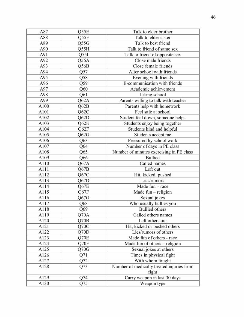
APPENDIX A: VARIABLE IDENTIFICATION
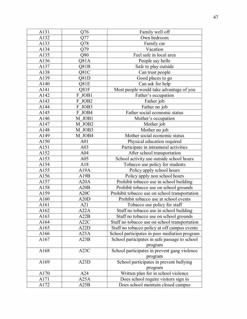
Parameter Question in Survey Meaning A1 Q1 Gender A2 Q4 Grade A3 IMP_AGE Imputed age A4 Q6 Race A5 Q10A Computer use, weekdays A6 Q10B Computer use, weekends A7 Q11 Number of computers at home A8 Q12 Internet connection at home A9 Q13A Never used internet A10 Q13B Age first used internet A11 Q14 Days a week involved in clubs/organizations A12 Q15A1 Mother in main home A13 Q15A2 Father in main home A14 Q15A3 Stepmother in main home A15 Q15A4 Stepfather in main home A16 Q15A5 Grandmother in main home A17 Q15A6 Grandfather in main home A18 Q15A7 Foster home as main home A19 Q15A8 Somewhere else as main home A20 Q15A9 Relatives in main home A21 Q15A10 Adult siblings in main home A22 Q15B1 Mother in second home A23 Q15B2 Father in second home A24 Q15B3 Stepmother in second home A25 Q15B4 Stepfather in second home A26 Q15B5 Grandmother in second home A27 Q15B6 Grandfather in second home A28 Q15B7 Foster home as second home A29 Q15B8 Somewhere else as second home A30 Q15B9 Relatives in second home A31 Q15B10 Adult siblings in second home A32 Q15A_BRO Number of brothers in main home A33 Q15A_SIS Number of sisters in main home A34 Q15B_BRO Number of brothers in second home A35 Q15B_SIS Number of sisters in second home A36 Q16A Time spent in main home A37 Q16B Time spent in second home A38 RESPADLT Adult who is responsible for care A39 SIBGUARD Sibling is responsible for care A40 Q17 Mother�s highest level of education A41 Q18 Father�s highest level of education A42 Q19A Watch TV, weekdays
Page 55
45
A43 Q19B Watch TV, weekends A44 Q20A Time spent on homework, weekdays A45 Q20B Time spent on homework, weekends A46 Q21 Physically active last 7 days A47 Q22 Physically active usual week A48 Q23A Breakfast weekdays A49 Q23B Breakfast weekends A50 Q24A Lunch weekdays A51 Q24B Lunch weekends A52 Q25A Supper weekdays A53 Q25B Supper weekends A54 Q27A Days eat breakfast at school A55 Q27B Days eat lunch at school A56 Q28E Days without lunch A57 Q29 How often go to school or bed hungry A58 BMI Body mass index A59 Q32 Think about looks A60 Q33 Think about body A61 Q34 On a diet A62 Q35 Weight control behavior last year A63 Q36A Weight control behavior � exercise A64 Q36B Weight control behavior � skip meals A65 A36C Weight control behavior - fasting A66 Q36D Weight control behavior � eat fewer sweets A67 Q36E Weight control behavior � eat less fat A68 Q36F Weight control behavior � drink less sodas A69 Q36G Weight control behavior � eat less A70 Q36H Weight control behavior � eat more fruits A71 Q36I Weight control behavior � drink more water A72 Q36J Weight control behavior � restrict to 1 food
group A73 Q36K Weight control behavior � vomiting A74 Q36L Weight control behavior � use pills A75 Q36M Weight control behavior � smoke more A76 Q36N Weight control behavior � professional care A77 Q36O Weight control behavior � other A78 Q41D Feeling low A79 Q41E Irritable or bad temper A80 Q41G Difficulties in sleeping A81 Q42 Health A82 Q43 Life satisfaction A83 Q55A Talk to father A84 Q55B Talk to step-father A85 Q55C Talk to mother A86 Q55D Talk to step-mother
Page 56
46
A87 Q55E Talk to elder brother A88 Q55F Talk to elder sister A89 Q55G Talk to best friend A90 Q55H Talk to friend of same sex A91 Q55I Talk to friend of opposite sex A92 Q56A Close male friends A93 Q56B Close female friends A94 Q57 After school with friends A95 Q58 Evening with friends A96 Q59 E-communication with friends A97 Q60 Academic achievement A98 Q61 Liking school A99 Q62A Parents willing to talk with teacher
A100 Q62B Parents help with homework A101 Q62C Feel safe at school A102 Q62D Student feel down, someone helps A103 Q62E Students enjoy being together A104 Q62F Students kind and helpful A105 Q62G Students accept me A106 Q63 Pressured by school work A107 Q64 Number of days in PE class A108 Q65 Number of minutes exercising in PE class A109 Q66 Bullied A110 Q67A Called names A111 Q67B Left out A112 Q67C Hit, kicked, pushed A113 Q67D Lies/rumors A114 Q67E Made fun � race A115 Q67F Made fun � religion A116 Q67G Sexual jokes A117 Q68 Who usually bullies you A118 Q69 Bullied others A119 Q70A Called others names A120 Q70B Left others out A121 Q70C Hit, kicked or pushed others A122 Q70D Lies/rumors of others A123 Q70E Made fun of others - race A124 Q70F Made fun of others � religion A125 Q70G Sexual jokes at others A126 Q71 Times in physical fight A127 Q72 With whom fought A128 Q73 Number of medically treated injuries from
fight A129 Q74 Carry weapon in last 30 days A130 Q75 Weapon type
Page 57
47
A131 Q76 Family well off A132 Q77 Own bedroom A133 Q78 Family car A134 Q79 Vacation A135 Q80 Feel safe in local area A136 Q81A People say hello A137 Q81B Safe to play outside A138 Q81C Can trust people A139 Q81D Good places to go A140 Q81E Can ask for help A141 Q81F Most people would take advantage of you A142 F_JOB1 Father�s occupation A143 F_JOB2 Father job A144 F_JOB3 Father no job A145 F_JOB4 Father social economic status A146 M_JOB1 Mother�s occupation A147 M_JOB2 Mother job A148 M_JOB3 Mother no job A149 M_JOB4 Mother social economic status A150 A01 Physical education required A151 A03 Participate in intramural activities A152 A04 After school transportation A153 A05 School activity use outside school hours A154 A18 Tobacco use policy for students A155 A19A Policy apply school hours A156 A19B Policy apply non school hours A157 A20A Prohibit tobacco use in school building A158 A20B Prohibit tobacco use on school grounds A159 A20C Prohibit tobacco use on school transportation A160 A20D Prohibit tobacco use at school events A161 A21 Tobacco use policy for staff A162 A22A Staff no tobacco use in school building A163 A22B Staff no tobacco use on school grounds A164 A22C Staff no tobacco use on school transportation A165 A22D Staff no tobacco policy at off campus events A166 A23A School participates in peer mediation programA167 A23B School participates in safe passage to school
program A168 A23C School participates in prevent gang violence
program A169 A23D School participates in prevent bullying
program A170 A24 Written plan for in school violence A171 A25A Does school require visitors sign in A172 A25B Does school maintain closed campus
Page 58
48
A173 A25C Implement staff or adult volunteers to monitor halls
A174 A25D Implement routine bag, desk locker checks A175 A25E Implement no carrying backpacks A176 A25F School implement wearing uniforms A177 A25G School implement id badges A178 A25H Implement mental detectors A179 A25I Implement police or security guards during
school day
Page 59
49
APPENDIX B: TOBACCO CODES
/*Tobacco Code for ordinal logistic regression with stepwise selection */ data thesis_tobacco; infile �C:\Users\Kori\Desktop\KLHM\Thesis\Feb 9\Codes\thesis_tobacco.txt�; input sub A1-A179; run; proc logistic data = thesis_tobacco; model sub=A1-A179/stepwise; run; /*Tobacco Code for principal component and Factor analyses*/ data thesis_tobacco2; infile �C:\Users\Kori\Desktop\KLHM\Thesis\Feb 9\Codes\thesis_tobacco.txt�; input sub A7 A8 A11 A12 A13 A16 A19 A29 A38 A41 A42 A45 A46 A48 A49 A50 A51 A54 A55 A56 A57 A59 A73 A76 A77 A78 A79 A80 A81 A82 A83 A84 A88 A92 A93 A95 A96 A97 A98 A99 A103 A109 A111 A116 A117 A119 A125 A126 A127 A128 A129 A130 A134 A143 A148 A155 A156 A157 A164 A166 A168 A174 A177;; run; proc factor data=thesis_tobacco2 simple method=prin priors=one mineigen=1 scree rotate=promax round flag=0.40; var A7 A8 A11 A12 A13 A16 A19 A29 A38 A41 A42 A45 A46 A48 A49 A50 A51 A54 A55 A56 A57 A59 A73 A76 A77 A78 A79 A80 A81 A82 A83 A84 A88 A92 A93 A95 A96 A97 A98 A99 A103 A109 A111 A116 A117 A119 A125 A126 A127 A128 A129 A130 A134 A143 A148 A155 A156 A157 A164 A166 A168 A174 A177; run; data thesis_drugs3; infile �C:\Users\Kori\Desktop\KLHM\Thesis\Feb 9\Codes\thesis_tobacco.txt�; input sub F1-F21; datalines; proc logistic data=thesis_tobacco3 descending; model sub=F1-F21; run;
Page 60
50
proc factor data=thesis_tobacco2 method=principal scree mineigen=0 priors=smc outstat=output1; run; proc factor data=output1 method=principal n=7 rotate=promax reorder score outstat=output2; run;
Page 61
51
APPENDIX C: TOBACCO RESULTS
Analysis of Maximum Likelihood Estimates
Parameter DF Estimate StandardError
Wald Chi-Square
Pr > ChiSq
Intercept 1 3.0831 1.7535 3.0916 0.0787
A7 1 0.0294 0.0105 7.8603 0.0051
A8 1 0.0612 0.0286 4.5977 0.0320
A11 1 -0.0305 0.00923 10.9429 0.0009
A12 1 -0.0294 0.0141 4.3433 0.0372
A13 1 -0.4309 0.0742 33.7097 <.0001
A16 1 0.3216 0.0649 24.5835 <.0001
A19 1 0.9620 0.3470 7.6849 0.0056
A29 1 -1.7399 0.7884 4.8697 0.0273
A38 1 -0.0760 0.0329 5.3422 0.0208
A41 1 0.0946 0.0207 20.8150 <.0001
A42 1 0.0753 0.0202 13.9298 0.0002
A45 1 0.1219 0.0217 31.3984 <.0001
A46 1 0.0421 0.0195 4.6513 0.0310
A48 1 -0.0337 0.0113 8.8483 0.0029
A49 1 0.0828 0.0124 44.3381 <.0001
A50 1 0.0767 0.0373 4.2251 0.0398
A51 1 0.0455 0.0172 6.9897 0.0082
A54 1 0.1298 0.0503 6.6629 0.0098
A55 1 -0.0472 0.0146 10.4215 0.0012
A56 1 -0.0485 0.0135 12.9447 0.0003
A57 1 -0.3248 0.0195 277.6717 <.0001
Page 62
52
Analysis of Maximum Likelihood Estimates
Parameter DF Estimate StandardError
Wald Chi-Square
Pr > ChiSq
A59 1 -0.0167 0.00584 8.1900 0.0042
A73 1 -0.4342 0.1130 14.7647 0.0001
A76 1 0.7212 0.1332 29.3315 <.0001
A77 1 -0.3926 0.1431 7.5311 0.0061
A78 1 -0.7847 0.1244 39.7927 <.0001
A79 1 0.0493 0.0202 5.9378 0.0148
A80 1 0.0737 0.0186 15.6357 <.0001
A81 1 0.0345 0.0169 4.1460 0.0417
A82 1 -0.1792 0.0353 25.7767 <.0001
A83 1 0.0439 0.0129 11.5128 0.0007
A84 1 -0.0930 0.0190 23.8267 <.0001
A88 1 0.0527 0.0159 10.9487 0.0009
A92 1 0.1695 0.0217 61.0734 <.0001
A93 1 -0.0592 0.0294 4.0472 0.0442
A95 1 -0.0346 0.0156 4.9538 0.0260
A96 1 -0.0590 0.0128 21.1141 <.0001
A97 1 -0.1100 0.0171 41.1930 <.0001
A98 1 -0.1546 0.0286 29.2033 <.0001
A99 1 -0.1517 0.0279 29.6395 <.0001
A103 1 -0.0575 0.0201 8.1577 0.0043
A109 1 0.0312 0.0146 4.5417 0.0331
A111 1 0.0960 0.0231 17.3370 <.0001
A116 1 0.1320 0.0351 14.1667 0.0002
A117 1 -0.0878 0.0241 13.2333 0.0003
Page 63
53
Analysis of Maximum Likelihood Estimates
Parameter DF Estimate StandardError
Wald Chi-Square
Pr > ChiSq
A119 1 -0.2147 0.0250 73.4457 <.0001
A125 1 0.2395 0.0430 30.9714 <.0001
A126 1 -0.1353 0.0329 16.9487 <.0001
A127 1 -0.0932 0.0241 15.0170 0.0001
A128 1 -0.0627 0.0110 32.3227 <.0001
A129 1 -0.0833 0.0356 5.4812 0.0192
A130 1 -0.1715 0.0203 71.6077 <.0001
A134 1 -0.1530 0.0471 10.5571 0.0012
A143 1 -0.0116 0.00435 7.0455 0.0079
A148 1 0.0975 0.0371 6.8818 0.0087
A155 1 1.1031 0.3725 8.7711 0.0031
A156 1 1.3158 0.6168 4.5514 0.0329
A157 1 -0.1475 0.0618 5.7018 0.0169
A164 1 -0.4447 0.0849 27.4231 <.0001
A166 1 0.1675 0.0716 5.4781 0.0193
A168 1 -0.1085 0.0538 4.0666 0.0437
A174 1 0.2546 0.0772 10.8600 0.0010
A177 1 -0.1106 0.0529 4.3655 0.0367
Eigenvalues of the Correlation Matrix
Eigenvalue Difference Proportion Cumulative
1 4.77743136 0.34336741 0.0758 0.0758
2 4.43406395 1.69001862 0.0704 0.1462
Page 64
54
Eigenvalues of the Correlation Matrix
Eigenvalue Difference Proportion Cumulative
3 2.74404533 0.58628424 0.0436 0.1898
4 2.15776109 0.12853068 0.0343 0.2240
5 2.02923040 0.42775883 0.0322 0.2562
6 1.60147158 0.01116348 0.0254 0.2817
7 1.59030810 0.09624339 0.0252 0.3069
8 1.49406472 0.01715070 0.0237 0.3306
9 1.47691401 0.08407063 0.0234 0.3541
10 1.39284339 0.05057465 0.0221 0.3762
11 1.34226874 0.11316146 0.0213 0.3975
12 1.22910728 0.05036859 0.0195 0.4170
13 1.17873869 0.02538314 0.0187 0.4357
14 1.15335554 0.02998182 0.0183 0.4540
15 1.12337372 0.03404649 0.0178 0.4718
16 1.08932723 0.01894874 0.0173 0.4891
17 1.07037849 0.01207277 0.0170 0.5061
18 1.05830572 0.01819488 0.0168 0.5229
19 1.04011084 0.02552561 0.0165 0.5394
20 1.01458523 0.00942632 0.0161 0.5555
21 1.00515892 0.01999829 0.0160 0.5715
22 0.98516062 0.00891491 0.0156 0.5871
23 0.97624571 0.01992015 0.0155 0.6026
24 0.95632556 0.02381732 0.0152 0.6178
Page 65
55
Eigenvalues of the Correlation Matrix
Eigenvalue Difference Proportion Cumulative
25 0.93250825 0.03181511 0.0148 0.6326
26 0.90069314 0.01920611 0.0143 0.6469
27 0.88148704 0.01200902 0.0140 0.6609
28 0.86947801 0.01317963 0.0138 0.6747
29 0.85629838 0.02127875 0.0136 0.6883
30 0.83501964 0.00724740 0.0133 0.7015
31 0.82777223 0.02460915 0.0131 0.7147
32 0.80316308 0.00334913 0.0127 0.7274
33 0.79981395 0.00477858 0.0127 0.7401
34 0.79503537 0.02204382 0.0126 0.7527
35 0.77299155 0.00786134 0.0123 0.7650
36 0.76513020 0.00828161 0.0121 0.7771
37 0.75684859 0.03072809 0.0120 0.7892
38 0.72612050 0.01402334 0.0115 0.8007
39 0.71209716 0.01033268 0.0113 0.8120
40 0.70176448 0.00874334 0.0111 0.8231
41 0.69302114 0.01286416 0.0110 0.8341
42 0.68015698 0.01001991 0.0108 0.8449
43 0.67013707 0.01599756 0.0106 0.8556
44 0.65413951 0.01918650 0.0104 0.8659
45 0.63495301 0.00183401 0.0101 0.8760
46 0.63311900 0.01667712 0.0100 0.8861
Page 66
56
Eigenvalues of the Correlation Matrix
Eigenvalue Difference Proportion Cumulative
47 0.61644188 0.01041028 0.0098 0.8959
48 0.60603160 0.01292285 0.0096 0.9055
49 0.59310874 0.02680961 0.0094 0.9149
50 0.56629913 0.01690249 0.0090 0.9239
51 0.54939665 0.03761497 0.0087 0.9326
52 0.51178168 0.00221490 0.0081 0.9407
53 0.50956678 0.01011451 0.0081 0.9488
54 0.49945227 0.01657449 0.0079 0.9567
55 0.48287778 0.01269391 0.0077 0.9644
56 0.47018387 0.01617348 0.0075 0.9719
57 0.45401040 0.05538967 0.0072 0.9791
58 0.39862072 0.08884947 0.0063 0.9854
59 0.30977125 0.00205836 0.0049 0.9903
60 0.30771289 0.17938989 0.0049 0.9952
61 0.12832300 0.02645920 0.0020 0.9972
62 0.10186380 0.02963072 0.0016 0.9989
63 0.07223308 0.0011 1.0000
Analysis of Maximum Likelihood Estimates
Page 67
57
Parameter DF Estimate StandardError
Wald Chi-Square
Pr > ChiSq
Intercept 1 1.1681 0.0243 2308.6187 <.0001
F1 1 -0.5818 0.0124 2184.9656 <.0001
F2 1 0.0933 0.00984 90.0364 <.0001
F3 1 0.1500 0.0135 124.3627 <.0001
F4 1 0.3823 0.0157 594.3277 <.0001
F5 1 -0.0679 0.0156 19.0476 <.0001
F6 1 0.0395 0.0182 4.7147 0.0299
F7 1 0.0744 0.0171 18.8841 <.0001
F8 1 -0.0178 0.0180 0.9821 0.3217
F9 1 0.0193 0.0179 1.1610 0.2813
F10 1 -0.0330 0.0185 3.1838 0.0744
F11 1 0.0682 0.0188 13.1417 0.0003
F12 1 0.0353 0.0202 3.0406 0.0812
F13 1 0.0525 0.0209 6.3206 0.0119
F14 1 -0.0210 0.0204 1.0573 0.3038
F15 1 -0.0442 0.0207 4.5322 0.0333
F16 1 0.0686 0.0208 10.9028 0.0010
F17 1 0.0707 0.0216 10.7129 0.0011
F18 1 0.1348 0.0217 38.5845 <.0001
F19 1 0.0140 0.0218 0.4130 0.5205
F20 1 0.0895 0.0234 14.6148 0.0001
F21 1 0.1164 0.0218 28.6258 <.0001
Page 68
58
Rotated Factor Pattern
Factor1 Factor2 Factor3 Factor4 Factor5 Factor6 Factor7
A77 0.94117 -0.00879 -0.01414 0.04689 0.07266 -0.07780 0.03417
A78 0.93815 0.02577 -0.02326 0.03855 0.06680 -0.09838 0.04099
A76 0.92671 -0.03851 0.03134 0.00583 0.08298 -0.06619 0.05097
A73 0.92134 -0.02003 0.00817 0.04123 0.06645 -0.04972 0.02632
A11 0.44204 -0.09241 -0.05064 0.04107 0.00445 0.00429 0.00269
A59 0.28973 0.02469 -0.18387 -0.02675 -0.14501 -0.00372 0.03232
A42 -0.18521 -0.01424 0.04638 -0.13533 0.18090 -0.03346 0.12345
A41 -0.24266 -0.00453 0.08118 -0.11169 0.23776 -0.01236 0.10103
A109 -0.28845 -0.01737 0.12478 0.09084 0.06034 0.11725 -0.01736
A125 -0.00882 0.75091 0.08553 -0.04900 -0.03866 -0.07231 -0.05386
A126 0.02490 0.72659 0.00308 0.03413 -0.00583 -0.02619 -0.09069
A116 -0.01327 0.67396 0.01129 -0.15175 0.01693 0.00803 -0.01633
A117 -0.03054 0.57123 -0.23099 -0.12977 0.10687 0.04835 0.03540
A129 -0.07347 0.56699 -0.15791 0.32827 -0.08192 0.01616 0.11037
A127 -0.10979 0.48976 -0.20751 0.40922 -0.09142 0.04212 0.07924
A119 -0.04999 0.48356 -0.17574 0.22983 -0.01195 -0.00351 -0.10784
A111 -0.09369 0.46875 -0.28265 -0.22681 0.10617 0.15951 0.02975
A130 -0.00089 0.45067 -0.10675 0.22101 -0.03116 0.01204 -0.07972
A57 0.06230 0.40764 -0.16013 0.23349 -0.07151 -0.14245 -0.03585
A29 0.00115 -0.11938 -0.04690 -0.00378 0.04134 0.07280 -0.03806
A19 -0.01709 -0.14797 -0.04582 0.02260 0.06691 0.08902 -0.02062
A79 0.01105 -0.12360 0.65951 0.09178 -0.12617 0.05833 -0.11294
Page 69
59
Rotated Factor Pattern
Factor1 Factor2 Factor3 Factor4 Factor5 Factor6 Factor7
A83 -0.06701 -0.09603 0.61980 0.10075 0.05775 0.13629 -0.00385
A80 0.04214 -0.10451 0.60133 -0.05334 -0.07012 0.01331 -0.08212
A81 0.05619 -0.10321 0.54285 0.00758 -0.11992 0.07019 -0.07467
A16 -0.02467 0.00963 0.16399 -0.08457 0.05257 -0.10046 0.02150
A38 0.04828 -0.05223 -0.09443 0.00473 -0.04179 0.04157 0.04383
A103 0.09393 0.21694 -0.24727 -0.07127 -0.07501 0.01227 -0.14244
A84 0.10757 -0.04258 -0.36844 -0.07657 -0.18487 -0.07405 0.07670
A98 0.05907 0.07156 -0.40848 0.11713 -0.19840 -0.01959 -0.19280
A99 0.08836 0.13199 -0.43850 0.13102 -0.07471 -0.05545 -0.21103
A82 0.14510 -0.03020 -0.52239 -0.13568 -0.09292 -0.14894 -0.03172
A96 0.06329 0.12392 0.04290 0.62662 -0.01850 -0.02371 0.01510
A95 -0.02719 0.05051 0.09151 0.62118 0.01940 0.02094 0.02086
A97 0.06848 -0.09392 -0.07223 0.44550 0.26129 -0.17183 0.06017
A128 -0.05893 0.27185 -0.23079 0.40674 -0.12480 0.11226 0.06764
A93 -0.03480 -0.05948 0.05882 0.39892 0.08111 0.05277 -0.04173
A48 -0.06193 -0.02577 0.13931 0.34206 0.26674 0.19288 0.04127
A88 0.04175 -0.15220 -0.13223 -0.17292 0.10878 0.07338 -0.04486
sub -0.26198 -0.17750 0.33208 -0.36477 0.13978 0.07714 0.09866
A92 -0.20865 0.00189 -0.01674 -0.45079 -0.16854 0.12093 -0.02421
A8 -0.05983 0.00678 -0.02381 0.11284 0.56109 -0.04861 -0.05526
A134 -0.01753 -0.16095 -0.00391 0.09354 0.43073 0.07821 -0.26749
A7 -0.00206 0.05769 -0.11716 0.19272 0.32331 -0.07560 0.08117
Page 70
60
Rotated Factor Pattern
Factor1 Factor2 Factor3 Factor4 Factor5 Factor6 Factor7
A174 -0.01956 -0.02964 0.02513 -0.02201 0.20970 -0.00568 -0.02051
A13 -0.01158 0.10911 -0.04783 0.03154 -0.13339 -0.08767 0.00758
A157 -0.08481 0.00291 0.00329 0.05068 -0.14560 -0.02480 0.07456
A148 -0.03990 0.06202 0.01495 -0.06147 -0.31095 -0.05227 0.08304
A12 -0.03950 0.04870 -0.12938 -0.18480 -0.42048 -0.08683 -0.12096
A143 -0.00078 -0.03417 -0.12924 -0.00296 -0.45324 -0.00855 0.04337
A51 -0.06391 -0.10882 0.08980 -0.01928 0.07825 0.68277 -0.04176
A56 -0.06323 0.01554 -0.04812 0.04502 -0.16937 0.63927 -0.02424
A49 -0.15811 0.01775 0.25223 -0.11322 0.11120 0.50134 0.05713
A50 -0.09196 -0.06795 0.22599 -0.10621 0.09773 0.41297 0.03930
A55 -0.09416 0.21422 0.00450 0.01674 -0.24257 0.40969 0.10733
A54 0.00081 -0.19426 0.08861 0.01529 0.18431 0.32575 -0.03886
A156 -0.06420 0.00895 0.01804 -0.02299 -0.00343 -0.07924 -0.05883
A46 0.07578 0.09270 0.09471 -0.20235 0.34220 -0.10396 0.53529
A45 -0.00601 0.05308 0.08237 -0.22760 0.35530 -0.04500 0.53248
A164 0.09298 -0.05382 -0.07549 0.10178 -0.18274 0.04792 0.48569
A155 -0.08460 -0.01498 0.00778 0.02859 -0.19729 -0.01324 0.45743
A166 0.08524 -0.01822 -0.03640 0.09464 -0.18813 0.05129 0.45561
A168 0.04154 -0.05794 -0.06406 0.02332 0.05993 0.11559 0.16083
A177 0.13490 -0.00045 -0.02356 -0.03634 0.09231 0.00414 -0.16034
Page 71
61
APPENDIX D: ALCOHOL CODES
/*Alcohol code for ordinal logistic regression with stepwise selection */ data thesis_alcohol; infile �C:\Users\Kori\Desktop\KLHM\Thesis\Feb 9\Codes\thesis_alcohol.txt�; input sub A1-A179; run; proc logistic data = thesis_alcohol; model sub =A1-A179/stepwise; run; /*Alcohol code for principal component and Factor analyses*/ data thesis_alcohol; infile �C:\Users\Kori\Desktop\KLHM\Thesis\Feb 9\Codes\thesis_alcohol.txt�; input sub A10 A20 A25 A36 A42 A46 A49 A52 A54 A56 A57 A62 A64 A76 A77 A78 A80 A81 A82 A83 A84 A87 A90 A92 A93 A95 A96 A97 A98 A99 A102 A110 A116 A117 A119 A124 A126 A127 A128 A130 A131 A134 A136 A140 A146 A148 A152 A157 A164 A170 A171 A176 A177; run; proc factor data=thesis_alcohol2 simple method=prin priors=one mineigen=1 scree rotate=promax round flag=0.40; var A10 A20 A25 A36 A42 A46 A49 A52 A54 A56 A57 A62 A64 A76 A77 A78 A80 A81 A82 A83 A84 A87 A90 A92 A93 A95 A96 A97 A98 A99 A102 A110 A116 A117 A119 A124 A126 A127 A128 A130 A131 A134 A136 A140 A146 A148 A152 A157 A164 A170 A171 A176 A177; run; data thesis_alcohol3; infile �C:\Users\Kori\Desktop\KLHM\Thesis\Feb 9\Codes\thesis_newalcohol.txt�; input sub F1-F17; datalines; proc logistic data=thesis_alcohol3 descending; model sub=F1-F17; run; proc factor data=thesis_alcohol2 method=principal scree mineigen=0 priors=smc outstat=output1; run; proc factor data=output1 method=principal n=11 rotate=promax reorder score outstat=output2; run;
Page 72
62
APPENDIX E: ALCOHOL RESULTS
Analysis of Maximum Likelihood Estimates
Parameter DF Estimate StandardError
Wald Chi-Square
Pr > ChiSq
Intercept 1 0.9843 0.6368 2.3888 0.1222
A10 1 -0.3411 0.0953 12.8037 0.0003
A20 1 0.5356 0.1985 7.2822 0.0070
A25 1 0.2549 0.0898 8.0566 0.0045
A36 1 0.0374 0.0125 8.9489 0.0028
A42 1 0.0938 0.0172 29.8603 <.0001
A46 1 0.0468 0.0148 10.0537 0.0015
A49 1 0.0538 0.0106 25.9290 <.0001
A52 1 0.0758 0.0367 4.2669 0.0389
A54 1 0.1247 0.0492 6.4169 0.0113
A56 1 0.0236 0.0106 4.9716 0.0258
A57 1 -0.4951 0.0221 502.8658 <.0001
A62 1 -0.0567 0.0181 9.7809 0.0018
A64 1 0.3095 0.0912 11.5257 0.0007
A76 1 0.4139 0.1349 9.4139 0.0022
A77 1 -0.3383 0.1359 6.1981 0.0128
A78 1 -1.0269 0.1232 69.4814 <.0001
A80 1 0.0602 0.0166 13.1268 0.0003
A81 1 0.0480 0.0155 9.6351 0.0019
A82 1 -0.0826 0.0328 6.3210 0.0119
A83 1 0.0369 0.0122 9.1153 0.0025
A84 1 -0.0340 0.0173 3.8667 0.0493
A87 1 -0.0626 0.0205 9.2885 0.0023
Page 73
63
Analysis of Maximum Likelihood Estimates
Parameter DF Estimate StandardError
Wald Chi-Square
Pr > ChiSq
A90 1 0.0561 0.0231 5.9071 0.0151
A92 1 0.1611 0.0205 61.7585 <.0001
A93 1 -0.0653 0.0262 6.2108 0.0127
A95 1 -0.0382 0.0140 7.4246 0.0064
A96 1 -0.0468 0.0119 15.4474 <.0001
A97 1 -0.0709 0.0155 20.9472 <.0001
A98 1 -0.0569 0.0266 4.5813 0.0323
A99 1 -0.1030 0.0264 15.1701 <.0001
A102 1 -0.0696 0.0201 11.9762 0.0005
A110 1 0.0853 0.0232 13.5621 0.0002
A116 1 0.1923 0.0331 33.6774 <.0001
A117 1 -0.0933 0.0223 17.5554 <.0001
A119 1 -0.2344 0.0248 89.5111 <.0001
A124 1 0.1549 0.0409 14.3537 0.0002
A126 1 -0.1211 0.0335 13.0279 0.0003
A127 1 -0.1246 0.0201 38.4094 <.0001
A128 1 -0.0575 0.0102 31.9120 <.0001
A130 1 -0.1559 0.0267 34.1436 <.0001
A131 1 -0.0756 0.0231 10.7131 0.0011
A134 1 -0.1906 0.0428 19.8482 <.0001
A136 1 -0.0685 0.0291 5.5454 0.0185
A140 1 -0.0447 0.0181 6.0727 0.0137
A146 1 0.0420 0.0171 6.0470 0.0139
A148 1 0.1067 0.0335 10.1272 0.0015
Page 74
64
Analysis of Maximum Likelihood Estimates
Parameter DF Estimate StandardError
Wald Chi-Square
Pr > ChiSq
A152 1 0.1067 0.0488 4.7786 0.0288
A157 1 -0.1331 0.0563 5.5897 0.0181
A164 1 -0.2452 0.0763 10.3335 0.0013
A170 1 0.1212 0.0457 7.0449 0.0079
A171 1 0.7220 0.2457 8.6314 0.0033
A176 1 -0.1187 0.0469 6.4153 0.0113
A177 1 0.1941 0.0477 16.5772 <.0001
Eigenvalues of the Correlation Matrix: Total = 53 Average = 1
Eigenvalue Difference Proportion Cumulative
1 4.58693518 1.06532191 0.0865 0.0865
2 3.52161327 1.01457369 0.0664 0.1530
3 2.50703957 0.44690348 0.0473 0.2003
4 2.06013610 0.41523431 0.0389 0.2392
5 1.64490179 0.12030771 0.0310 0.2702
6 1.52459408 0.13140887 0.0288 0.2990
7 1.39318521 0.06425195 0.0263 0.3253
8 1.32893326 0.07759428 0.0251 0.3503
9 1.25133898 0.02682217 0.0236 0.3739
10 1.22451680 0.03763071 0.0231 0.3970
11 1.18688609 0.07539852 0.0224 0.4194
Page 75
65
Eigenvalues of the Correlation Matrix: Total = 53 Average = 1
Eigenvalue Difference Proportion Cumulative
12 1.11148757 0.04597904 0.0210 0.4404
13 1.06550853 0.01169637 0.0201 0.4605
14 1.05381216 0.02251054 0.0199 0.4804
15 1.03130162 0.00518833 0.0195 0.4999
16 1.02611329 0.01120564 0.0194 0.5192
17 1.01490764 0.01736782 0.0191 0.5384
18 0.99753982 0.01630677 0.0188 0.5572
19 0.98123305 0.02555539 0.0185 0.5757
20 0.95567766 0.01963430 0.0180 0.5937
21 0.93604336 0.01392043 0.0177 0.6114
22 0.92212293 0.01334383 0.0174 0.6288
23 0.90877910 0.01315857 0.0171 0.6459
24 0.89562054 0.02564151 0.0169 0.6628
25 0.86997903 0.02264608 0.0164 0.6792
26 0.84733295 0.02977278 0.0160 0.6952
27 0.81756017 0.00209847 0.0154 0.7107
28 0.81546170 0.01255065 0.0154 0.7260
29 0.80291104 0.00840437 0.0151 0.7412
30 0.79450667 0.00563199 0.0150 0.7562
31 0.78887468 0.02385157 0.0149 0.7711
32 0.76502311 0.00412686 0.0144 0.7855
Page 76
66
Eigenvalues of the Correlation Matrix: Total = 53 Average = 1
Eigenvalue Difference Proportion Cumulative
33 0.76089626 0.00901511 0.0144 0.7999
34 0.75188115 0.02546606 0.0142 0.8141
35 0.72641509 0.00950732 0.0137 0.8278
36 0.71690777 0.03635641 0.0135 0.8413
37 0.68055135 0.00415961 0.0128 0.8541
38 0.67639175 0.00951696 0.0128 0.8669
39 0.66687479 0.01040997 0.0126 0.8795
40 0.65646482 0.01556376 0.0124 0.8919
41 0.64090106 0.02567999 0.0121 0.9039
42 0.61522107 0.03593067 0.0116 0.9156
43 0.57929040 0.01703823 0.0109 0.9265
44 0.56225217 0.01585284 0.0106 0.9371
45 0.54639933 0.00360007 0.0103 0.9474
46 0.54279926 0.00839773 0.0102 0.9576
47 0.53440153 0.07494693 0.0101 0.9677
48 0.45945459 0.00633022 0.0087 0.9764
49 0.45312437 0.12710949 0.0085 0.9849
50 0.32601488 0.02945675 0.0062 0.9911
51 0.29655814 0.19564247 0.0056 0.9967
52 0.10091566 0.02650805 0.0019 0.9986
53 0.07440761 0.0014 1.0000
Page 77
67
Analysis of Maximum Likelihood Estimates
Parameter DF Estimate StandardError
Wald Chi-Square
Pr > ChiSq
Intercept 1 0.4016 0.0206 381.7310 <.0001
F1 1 0.4792 0.0115 1724.2675 <.0001
F2 1 0.2530 0.0108 552.0730 <.0001
F3 1 0.2526 0.0134 357.3324 <.0001
F4 1 0.2088 0.0145 206.4757 <.0001
F5 1 0.1082 0.0158 46.7076 <.0001
F6 1 0.0277 0.0165 2.8161 0.0933
F7 1 0.1105 0.0179 38.1329 <.0001
F8 1 -0.0850 0.0177 22.9452 <.0001
F9 1 0.1432 0.0184 60.2898 <.0001
F10 1 0.0340 0.0184 3.4364 0.0638
F11 1 0.0954 0.0188 25.8205 <.0001
F12 1 0.0261 0.0195 1.8030 0.1794
F13 1 0.00419 0.0199 0.0444 0.8331
F14 1 0.0437 0.0200 4.7944 0.0286
F15 1 0.00438 0.0201 0.0476 0.8273
F16 1 0.0520 0.0201 6.6967 0.0097
F17 1 0.1495 0.0202 54.7736 <.0001
Page 78
68
APPENDIX F: DRUG CODES
/*Drugs Code for ordinal logistic regression with stepwise selection*/ data thesis_drugs; infile �C:\Users\Kori\Desktop\KLHM\Thesis\Feb 9\Codes\thesis_drugs.txt�; input sub A1-A179; run; proc logistic data = thesis_drugs; model sub =A1-A179/stepwise; run; /*Drugs Code for principal component and Factor analyses*/ data thesis_drugs; infile �C:\Users\Kori\Desktop\KLHM\Thesis\Feb 9\Codes\thesis_drugs.txt�; input sub A2 A7 A12 A14 A15 A20 A40 A41 A45 A49 A52 A55 A57 A61 A64 A69 A74 A75 A76 A77 A80 A83 A88 A92 A96 A98 A110 A112 A117 A119 A127 A129 A137 A152 A168; run; proc factor data=thesis_drugs2 simple method=prin priors=one mineigen=1 scree rotate=promax round flag=0.40; var A2 A7 A12 A14 A15 A20 A40 A41 A45 A49 A52 A55 A57 A61 A64 A69 A74 A75 A76 A77 A80 A83 A88 A92 A96 A98 A110 A112 A117 A119 A127 A129 A137 A152 A168; run; data thesis_drugs3; infile �C:\Users\Kori\Desktop\KLHM\Thesis\Feb 9\Codes\thesis_newdrugs.txt�; input sub F1-F12; datalines; proc logistic data=thesis_drugs3 descending; model sub=F1-F12; run; proc factor data=thesis_drugs2 method=principal scree mineigen=0 priors=smc outstat=output1; run; proc factor data=output1 method=principal n=5 rotate=promax reorder score outstat=output2; run;
Page 79
69
APPENDIX G: DRUG RESULTS
Analysis of Maximum Likelihood Estimates
Parameter DF Estimate StandardError
Wald Chi-Square
Pr > ChiSq
Intercept 1 -0.3026 1.2959 0.0545 0.8153
A2 1 0.0621 0.0248 6.2692 0.0123
A7 1 0.0399 0.0158 6.3863 0.0115
A12 1 -0.0668 0.0211 10.0147 0.0016
A14 1 -0.3900 0.0755 26.7006 <.0001
A15 1 0.5890 0.1998 8.6941 0.0032
A20 1 0.6747 0.3179 4.5044 0.0338
A40 1 -0.9471 0.4552 4.3285 0.0375
A41 1 0.1066 0.0303 12.3514 0.0004
A45 1 0.1421 0.0279 25.9871 <.0001
A49 1 0.0513 0.0187 7.5369 0.0060
A52 1 0.1254 0.0599 4.3854 0.0362
A55 1 -0.0791 0.0254 9.7240 0.0018
A57 1 -0.4305 0.0321 180.0042 <.0001
A61 1 0.1245 0.0474 6.9139 0.0086
A64 1 0.2320 0.1045 4.9258 0.0265
A69 1 -0.1931 0.0790 5.9690 0.0146
A74 1 -0.4093 0.1720 5.6603 0.0174
A75 1 0.4111 0.1529 7.2309 0.0072
A76 1 0.9189 0.1414 42.2428 <.0001
A77 1 -0.5566 0.1701 10.7038 0.0011
A80 1 0.0798 0.0281 8.0925 0.0044
Page 80
70
Analysis of Maximum Likelihood Estimates
Parameter DF Estimate StandardError
Wald Chi-Square
Pr > ChiSq
A83 1 0.0672 0.0205 10.7566 0.0010
A88 1 0.0641 0.0245 6.8605 0.0088
A92 1 0.2070 0.0367 31.8931 <.0001
A96 1 -0.1214 0.0176 47.3702 <.0001
A98 1 -0.2990 0.0447 44.7567 <.0001
A110 1 0.1239 0.0476 6.7836 0.0092
A112 1 0.0957 0.0460 4.3219 0.0376
A117 1 -0.1168 0.0379 9.4832 0.0021
A119 1 -0.2092 0.0404 26.7524 <.0001
A127 1 -0.1443 0.0411 12.3151 0.0004
A129 1 -0.2246 0.0633 12.5696 0.0004
A137 1 -0.0870 0.0317 7.5270 0.0061
A152 1 0.1599 0.0769 4.3262 0.0375
A168 1 -0.2040 0.0875 5.4363 0.0197
Eigenvalues of the Correlation Matrix: Total = 35 Average = 1
Eigenvalue Difference Proportion Cumulative
1 3.67243602 1.40135528 0.1049 0.1049
2 2.27108074 0.52180185 0.0649 0.1698
3 1.74927889 0.07197903 0.0500 0.2198
4 1.67729986 0.23344448 0.0479 0.2677
Page 81
71
Eigenvalues of the Correlation Matrix: Total = 35 Average = 1
Eigenvalue Difference Proportion Cumulative
5 1.44385538 0.20564210 0.0413 0.3090
6 1.23821328 0.08596923 0.0354 0.3443
7 1.15224405 0.00947248 0.0329 0.3773
8 1.14277157 0.04760717 0.0327 0.4099
9 1.09516439 0.02362355 0.0313 0.4412
10 1.07154084 0.04118606 0.0306 0.4718
11 1.03035478 0.01491902 0.0294 0.5013
12 1.01543576 0.01565065 0.0290 0.5303
13 0.99978511 0.04592966 0.0286 0.5588
14 0.95385546 0.01001191 0.0273 0.5861
15 0.94384354 0.01806367 0.0270 0.6131
16 0.92577987 0.01030819 0.0265 0.6395
17 0.91547168 0.02940704 0.0262 0.6657
18 0.88606465 0.02223907 0.0253 0.6910
19 0.86382557 0.03695763 0.0247 0.7157
20 0.82686794 0.01922287 0.0236 0.7393
21 0.80764507 0.01980506 0.0231 0.7624
22 0.78784001 0.01015477 0.0225 0.7849
23 0.77768524 0.03419319 0.0222 0.8071
24 0.74349205 0.03238797 0.0212 0.8283
25 0.71110408 0.03099006 0.0203 0.8487
Page 82
72
Eigenvalues of the Correlation Matrix: Total = 35 Average = 1
Eigenvalue Difference Proportion Cumulative
26 0.68011402 0.00676535 0.0194 0.8681
27 0.67334867 0.01972892 0.0192 0.8873
28 0.65361975 0.02458944 0.0187 0.9060
29 0.62903031 0.05750927 0.0180 0.9240
30 0.57152104 0.07724059 0.0163 0.9403
31 0.49428045 0.00956640 0.0141 0.9544
32 0.48471405 0.04493715 0.0138 0.9683
33 0.43977690 0.05407473 0.0126 0.9808
34 0.38570217 0.10074540 0.0110 0.9919
35 0.28495677 0.0081 1.0000
Analysis of Maximum Likelihood Estimates
Parameter DF Estimate StandardError
Wald Chi-Square
Pr > ChiSq
Intercept 1 0.7604 0.0363 438.5033 <.0001
F1 1 0.5312 0.0217 599.0716 <.0001
F2 1 -0.3403 0.0239 202.7421 <.0001
F3 1 -0.5000 0.0289 300.2685 <.0001
F4 1 0.2190 0.0275 63.5307 <.0001
F5 1 -0.0960 0.0295 10.5994 0.0011
F6 1 -0.0383 0.0317 1.4566 0.2275
Page 83
73
Analysis of Maximum Likelihood Estimates
Parameter DF Estimate StandardError
Wald Chi-Square
Pr > ChiSq
F7 1 0.1559 0.0331 22.1205 <.0001
F8 1 0.0198 0.0326 0.3689 0.5436
F9 1 0.1415 0.0332 18.1257 <.0001
F10 1 0.1617 0.0350 21.3972 <.0001
F11 1 -0.0403 0.0353 1.3038 0.2535
F12 1 0.0501 0.0349 2.0618 0.1510
Rotated Factor Pattern
Factor1 Factor2 Factor3 Factor4 Factor5
A74 0.81293 -0.08546 -0.04866 0.03140 -0.00831
A75 0.80727 -0.09576 -0.05507 0.10409 0.02624
A77 0.78949 0.00686 0.01947 -0.08727 -0.04445
A76 0.72325 -0.26473 0.00558 0.09648 -0.04143
A40 -0.04268 -0.00176 0.00893 0.00523 -0.03778
A127 -0.05751 0.68757 0.23905 -0.04903 0.01833
A129 -0.11376 0.64890 0.29515 0.00954 0.06085
A57 -0.15711 0.56764 0.09079 -0.20853 0.00952
A96 0.06081 0.51271 -0.18131 -0.02093 -0.23587
A119 -0.06273 0.45958 0.30278 -0.09489 -0.02692
A15 -0.02130 -0.06128 -0.04266 0.05659 -0.03662
Page 84
74
Rotated Factor Pattern
Factor1 Factor2 Factor3 Factor4 Factor5
A88 0.03419 -0.26159 0.10597 -0.10688 0.02488
A45 -0.02318 -0.28011 0.17449 0.24487 -0.16902
sub 0.07758 -0.58113 0.03693 0.32306 -0.03936
A112 -0.10185 0.06111 0.74867 -0.00028 0.07097
A110 -0.07394 0.10681 0.72470 0.01270 0.04388
A117 -0.12815 0.13732 0.66334 -0.03919 -0.00778
A7 0.08788 0.03613 0.17871 0.06422 -0.10133
A2 0.01771 -0.02992 0.07372 -0.00937 -0.01844
A83 0.05319 -0.01730 -0.31846 0.57722 -0.11053
A49 -0.05383 -0.01311 0.01566 0.56128 0.08543
A80 0.12875 -0.13452 -0.26249 0.43941 0.05638
A55 -0.07683 0.22139 0.14411 0.32757 0.23844
A41 0.01323 0.00566 0.09995 0.29872 -0.09724
A52 0.05776 -0.06349 -0.10703 0.26065 0.13179
A20 -0.00891 -0.04025 0.04866 0.15186 0.02697
A14 -0.01950 0.12805 -0.02662 -0.18706 0.12788
A137 0.00067 -0.02062 0.20628 -0.24827 0.22321
A61 -0.07648 -0.21628 0.16912 -0.38695 -0.34940
A98 -0.04524 0.21939 -0.00321 -0.45022 0.25197
A64 0.15030 0.04489 0.01558 -0.04557 0.58336
A12 -0.05795 -0.00097 -0.06012 -0.33096 0.53729
A69 0.36995 0.24753 -0.02644 0.06095 0.43784
Page 85
75
Rotated Factor Pattern
Factor1 Factor2 Factor3 Factor4 Factor5
A92 -0.05674 -0.32558 0.18219 0.04976 0.41295
A152 0.04643 0.04637 0.03889 0.00433 -0.19639
A168 -0.00149 -0.00401 -0.00569 -0.04406 -0.19892