96
MATH6501 Mathematics for Engineers 1 Department of Mathematics, University College London BelginSeymeno˘glu e-mail: [email protected] Autumn 2016
MATH6501 Mathematics for Engineers 1
Department of Mathematics,
University College London
Belgin Seymenoglue-mail: [email protected]
Autumn 2016

Contents
1 Differentiation 2
1.1 Introduction . . . . . . . . . . . . . . . . . . . . . . . . . . . . . . . . . . . . 2
1.2 Basic differentiation . . . . . . . . . . . . . . . . . . . . . . . . . . . . . . . 3
1.3 The Chain Rule . . . . . . . . . . . . . . . . . . . . . . . . . . . . . . . . . . 5
1.3.1 Implicit differentiation . . . . . . . . . . . . . . . . . . . . . . . . . . 7
1.4 Higher derivatives . . . . . . . . . . . . . . . . . . . . . . . . . . . . . . . . 9
1.4.1 Computing the nth derivative of a product . . . . . . . . . . . . . . 10
1.4.2 Parametric differentiation . . . . . . . . . . . . . . . . . . . . . . . . 12
1.5 Using differentiation . . . . . . . . . . . . . . . . . . . . . . . . . . . . . . . 13
1.5.1 Finding stationary points . . . . . . . . . . . . . . . . . . . . . . . . 13
1.5.2 Curve sketching . . . . . . . . . . . . . . . . . . . . . . . . . . . . . . 16
1.5.3 Equations of Tangent and Normal . . . . . . . . . . . . . . . . . . . 20
2 Hyperbolic functions 22
2.1 Definitions of hyperbolic functions . . . . . . . . . . . . . . . . . . . . . . . 22
2.2 Inverse hyperbolic functions . . . . . . . . . . . . . . . . . . . . . . . . . . . 24
2.3 Hyperbolic identities . . . . . . . . . . . . . . . . . . . . . . . . . . . . . . . 25
3 Partial differentiation 28
3.1 Introduction to partial differentiation . . . . . . . . . . . . . . . . . . . . . . 28
3.2 Higher Partial Derivatives . . . . . . . . . . . . . . . . . . . . . . . . . . . . 32
i
CONTENTS ii
4 Integration 35
4.1 The basics . . . . . . . . . . . . . . . . . . . . . . . . . . . . . . . . . . . . . 35
4.2 Integration by substitution . . . . . . . . . . . . . . . . . . . . . . . . . . . 37
4.2.1 A question of logs . . . . . . . . . . . . . . . . . . . . . . . . . . . . 38
4.2.2 Trigonometric and hyperbolic substitutions . . . . . . . . . . . . . . 39
4.2.3 One more trick . . . . . . . . . . . . . . . . . . . . . . . . . . . . . . 40
4.3 Integration by parts . . . . . . . . . . . . . . . . . . . . . . . . . . . . . . . 41
4.4 Using partial fractions . . . . . . . . . . . . . . . . . . . . . . . . . . . . . . 43
4.4.1 Recap: Partial fractions . . . . . . . . . . . . . . . . . . . . . . . . . 43
4.5 Some trigonometric integrals . . . . . . . . . . . . . . . . . . . . . . . . . . 46
4.6 Using integration . . . . . . . . . . . . . . . . . . . . . . . . . . . . . . . . . 46
4.7 Improper integrals . . . . . . . . . . . . . . . . . . . . . . . . . . . . . . . . 50
5 Differential Equations 51
5.1 Introduction . . . . . . . . . . . . . . . . . . . . . . . . . . . . . . . . . . . . 51
5.2 First order separable ODEs . . . . . . . . . . . . . . . . . . . . . . . . . . . 53
5.3 First order linear ODEs . . . . . . . . . . . . . . . . . . . . . . . . . . . . . 55
5.4 Initial Value Problems . . . . . . . . . . . . . . . . . . . . . . . . . . . . . . 58
6 Vectors 61
6.1 Introduction . . . . . . . . . . . . . . . . . . . . . . . . . . . . . . . . . . . . 61
6.2 The Dot Product . . . . . . . . . . . . . . . . . . . . . . . . . . . . . . . . . 64
6.3 The Cross Product . . . . . . . . . . . . . . . . . . . . . . . . . . . . . . . . 67
7 Numerical Methods 71
7.1 Introduction . . . . . . . . . . . . . . . . . . . . . . . . . . . . . . . . . . . . 71
7.2 The Rectangular Rule . . . . . . . . . . . . . . . . . . . . . . . . . . . . . . 72
7.3 The Trapezium Rule . . . . . . . . . . . . . . . . . . . . . . . . . . . . . . . 72
7.4 Simpson’s Rule . . . . . . . . . . . . . . . . . . . . . . . . . . . . . . . . . . 75

CONTENTS iii
7.5 Newton’s Method for Root-Finding . . . . . . . . . . . . . . . . . . . . . . . 77
8 Probability and Statistics 81
8.1 Basic Probability . . . . . . . . . . . . . . . . . . . . . . . . . . . . . . . . . 81
8.2 Random Variables . . . . . . . . . . . . . . . . . . . . . . . . . . . . . . . . 85
8.3 The Binomial Distribution . . . . . . . . . . . . . . . . . . . . . . . . . . . . 88
8.4 The Poisson Distribution . . . . . . . . . . . . . . . . . . . . . . . . . . . . 90

Acknowledgements
These lecture notes are largely an upgraded version of the notes produced by Alex White,which in turn are based on the notes of Professor Robb McDonald. The LaTeX code whichAlex used to make his notes eventually made their way into my hands, without which itwould have been much harder to typeset this version of the lecture notes.
Many years later, Anna Lambert became the previous lecturer for this course. Manythanks goes to Anna for passing on her experience in teaching the course to me. Withher advice in mind, I have made removed some content from Alex’s notes which no longerbelongs on the syllabus.
Some of the content in these notes is also based on two other courses taught by theUCL Maths Department: MATH1403 (Mathematical Methods for Arts and Sciences) andMATH6103 (Differential and Integral Calculus). The lecture notes for these two courseswere kindly shared by Adam Townsend and Matthew Scroggs respectively. Moreover,Adam attended one of my lectures and subsequently offered some constructive advice forimproving the content of the course, while Matthew patiently helped me to debug theLaTeX code. As a result, I am immensely grateful to them both for all their assistance.
I would also like to thank Oliver Southwick for his useful discussion about the chapter onvectors; his perspective of the dot product has been a major influence in the writing up ofSection 6.2 of these notes.
1

Chapter 1
Differentiation
1.1 Introduction
Why differentiation? Well, it is a useful tool because many real-world problems rely on therates of change of quantities. For example, speed is the rate of change of distance of amoving object.
Sometimes an engineer will need to look at a graph of, for example, distance vs time. Inthat case, questions about rate of change become questions about gradients, i.e. slopes ofthe tangent to a curve.
Slope of the chord PQ
=Change in y
Change in x=f(x+ δx)− f(x)
δx,
and as δx→ 0, chord → tangent.
Therefore: Slope of the tangent at x
=dy
dx= lim
δx→0
(f(x+ δx)− f(x)
δx
).
2
CHAPTER 1. DIFFERENTIATION 3
Example 1.1. Use the above definition to differentiate y = f(x) = x2.
dy
dx= lim
δx→0
((x+ δx)2 − x2
δx
)= lim
δx→0
(��x
2 + 2xδx+ (δx)2 −��x2
δx
)= lim
δx→0(2x+ δx)
= 2x.
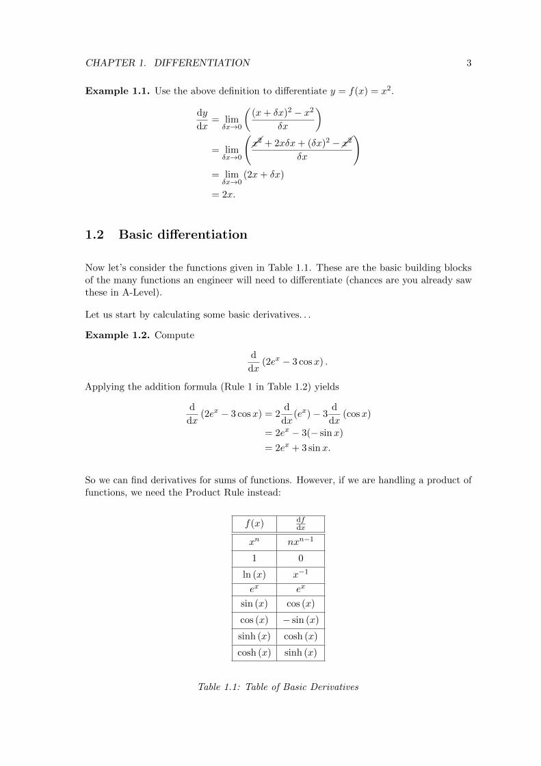
1.2 Basic differentiation
Now let’s consider the functions given in Table 1.1. These are the basic building blocksof the many functions an engineer will need to differentiate (chances are you already sawthese in A-Level).
Let us start by calculating some basic derivatives. . .
Example 1.2. Compute
d
dx(2ex − 3 cosx) .
Applying the addition formula (Rule 1 in Table 1.2) yields
d
dx(2ex − 3 cosx) = 2
d
dx(ex)− 3
d
dx(cosx)
= 2ex − 3(− sinx)
= 2ex + 3 sinx.
So we can find derivatives for sums of functions. However, if we are handling a product offunctions, we need the Product Rule instead:
f(x) dfdx
xn nxn−1
1 0
ln (x) x−1
ex ex
sin (x) cos (x)
cos (x) − sin (x)
sinh (x) cosh (x)
cosh (x) sinh (x)
Table 1.1: Table of Basic Derivatives

CHAPTER 1. DIFFERENTIATION 4
Rule f(x) dfdx Notes
1 u+ v dudx + dv
dx Addition Rule
2 Cu C dudx (C =constant)
3 uv v dudx + udv
dx Product Rule
4 u/vv dudx−u dv
dxv2
Quotient Rule
5 f(u(x)) f ′(u(x))dudx Chain Rule
6 dxdy
1dydx
For Inverse Functions
Table 1.2: Table of Rules for Differentiation
Example 1.3. Computed
dx
(x3 sinx
).
This is a product of two functions, hence the Product Rule is required (Rule 3 in Table 2).This is:
d
dx(uv) = v
du
dx+ u
dv
dx.
For this example, let u = x3 and v = sinx. Then we have. . .
d
dx
(x3 sinx
)=
d
dx
(x3)
sinx+ x3 d
dx(sinx) ,
i.e.d
dx
(x3 sinx
)= 3x2 sinx+ x3 cosx.
The Product Rule still works if you want to compute the derivative of a function that is aproduct of three or more functions.
Example 1.4. Compute
d
dx
(x2ex sinx
)=
d
dx
(x2)ex sinx
+ x2 d
dx(ex) sinx
+ x2exd
dx(sinx)
= (2xex + x2ex) sinx+ x2ex cosx.
This next example shows a standard use of the Quotient Rule:
Example 1.5. Computed
dx
(x− 1
x2 + 1
).

CHAPTER 1. DIFFERENTIATION 5
Applying the Quotient Rule gives
d
dx
(x− 1
x2 + 1
)=
(x2 + 1
)d
dx (x− 1)− (x− 1) ddx
(x2 + 1
)(x2 + 1)2
=
(x2 + 1
)× 1− (x− 1)× 2x
(x2 + 1)2
=−x2 + 2x+ 1
(x2 + 1)2 .
Example 1.6 (Differentiate tanhx using the quotient rule).
d
dx(tanhx) =
d
dx
(sinhx
coshx
)=
coshx ddx (sinhx)− sinhx d
dx (coshx)
cosh2 x
=cosh× coshx− sinhx× sinhx
cosh2 x
=cosh2 x− sinh2 x
cosh2 x,
and now using the hyperbolic identity
cosh2 x− sinh2 x ≡ 1,
this leads to
d
dx(tanhx) =
1
cosh2 x,
and since
sechx ≡ 1
coshx=⇒ sech2 x ≡ 1
cosh2 x,
this leads to the resultd
dx(tanhx) = sech2 x.
This looks very similar to the following result. . .
d
dx(tanx) = sec2 x,
which uses the trigonometric functions instead of hyperbolic ones. You will get to provethis result for yourself in the Problem Sheet!
1.3 The Chain Rule
So far, we have calculated derivatives of sums, products and quotients of functions. Butwhat happens when you have a function of a function?
CHAPTER 1. DIFFERENTIATION 6
Example 1.7. Compute the following derivative
d
dx(sin 2x) .
The Chain Rule says thatd
dx(f(u(x))) = f ′(u(x))
du
dx.
So we let
u(x) = 2x,du
dx= 2,
f(u) = sinudf
du= cosu
then applying the chain rule gives
d
dx(sin 2x) =
d
du(f(u))
du
dx= 2 cosu,
and rewriting back in terms of the original variable x gives
d
dx(sin 2x) = 2 cos 2x.
Let’s try another example. . .
Example 1.8. Compute the following derivative
d
dx
(ln(x2 − 1
)).
Put
u(x) = x2 − 1, u′(x) = 2x,
f(u) = lnu, f ′(u) =1
u,
then applying the chain rule gives
d
dx
(ln(x2 − 1
))=
2x
u=
2x
x2 − 1.
You will want to brace yourself for the next example! This one shows you how to use thechain rule more than once.
Example 1.9. Compute the following derivative
d
dx
(sin(ln(x2ex
)))First apply chain rule with f(u) = sinu, u = ln
(x2ex
)= cos
(ln(x2ex
))× d
dx
(ln(x2ex
))Then apply chain rule again, this time with f(u) = lnu, u = x2ex
= cos(ln(x2ex
)) 1
x2exd
dx
(x2ex
)Finally, apply the product rule with u = x2, v = ex
= cos(ln(x2ex
)) 1
x2ex[x2ex + 2xex
].
CHAPTER 1. DIFFERENTIATION 7
Example 1.10 (2009 Exam Question). Compute the following derivative:
dy
dxfor y = sin
(e−x
x
).
This problem requires the chain rule with
f(u) = sinu,df
du= cosu,
u =e−x
x,
du
dx= −e
−x
x− e−x
x2.
Hencedy
dx= cos
(e−x
x
)(−e−x
x− e−x
x2
).
1.3.1 Implicit differentiation
Sometimes you can’t write a function in terms of x only. In that case, if you are differenti-ating w.r.t. x, you use implicit differentiation.
Example 1.11 (Slope of a circle with radius 1). Suppose x2 + y2 = 1.
• This is the equation of a circle, centre O, radius 1.
• y is an implicit function of x, i.e. not in the form
y = Stuff depending onx only
• To find dydx we take d
dx of all terms:
d
dx
(x2)
+d
dx
(y2)
=d
dx(1) ,
i.e
2x+ 2ydy
dx= 0 ∴
dy
dx= −x
y.
Example 1.12. If the equation of a curve satisfies
x2 + 3xy + y2 = 7,
find dydx in terms of x and y.
Proceed by differentiating each term w.r.t. x:
2x+ 3y + 3xdy
dx+ 2y
dy
dx= 0
(Common error: Forgetting to differentiate the 7!)
i.edy
dx= −2x+ 3y
3x+ 2y.

CHAPTER 1. DIFFERENTIATION 8
Logarithmic differentiation
Sometimes it is useful to take logs on both sides of an equation before differentiating. Bydoing this you are setting up an implicit equation, making this an example of implicitdifferentiation.
Example 1.13. Differentiate the function y = 10x with respect to x.
y = 10x, ∴ ln y = x ln 10.
and so in differentiating w.r.t x
1
y
dy
dx= ln 10,
dy
dx= 10x ln 10.
Example 1.14. Findd
dx(xx) .
First let y = xx, then ln y = lnxx = x lnx.
d
dx(ln y) =
d
dx(x lnx)
⇒ 1
y
dy
dx= lnx+
�x
�x
⇒ dy
dx= y (1 + lnx)
∴dy
dx= xx (1 + lnx) .
Example 1.15.
y =x2 cosx
sin 2x
(=
x2
2 sinx
).
Take logs and differentiate with respect to x to give
ln y = lnx2 + ln cosx− ln sin 2x
1
y
dy
dx=
2x
x2− sinx
cosx− 2
cos 2x
sin 2x.
∴dy
dx= y
(2
x− tanx− 2 cot 2x
)dy
dx=
x2 cosx
sin 2x
(2
x− tanx− 2 cot 2x
).
Differentiating Inverse functions
Believe it or not, when you differentiate an inverse function, you are using implicitdifferentiation (again!)

CHAPTER 1. DIFFERENTIATION 9
Example 1.16.
Finddy
dxwhen y = sin−1 x.
y = sin−1 x
sin y = x
d
dx(sin y) = 1
cos ydy
dx= 1
dy
dx=
1
cos y=
1√1− x2
.
Example 1.17.
Finddy
dxwhen y = cosh−1 x.
y = cosh−1 x
x = cosh y
1 = sinh ydy
dx(Implicit differentiation)
dy
dx=
1
sinh y
=1√
cosh2 y − 1(cosh2 y − sinh2 y ≡ 1)
=1√
x2 − 1.
Thereforedy
dx=
1√x2 − 1
.
1.4 Higher derivatives
Having founddy
dx, we can differentiate this again, which gives the second derivative
d2y
dx2. If
we then differentiate again, we getd3y
dx3,
d4y
dx4, etc. These are collectively known as higher
derivatives.
CHAPTER 1. DIFFERENTIATION 10
Example 1.18.
y = x6
dy
dx= 6x5
d2y
dx2= 6× 5x4 = 30x4
d3y
dx3= 30× 4x3 = 120x3
d4y
dx4= 360x2
d5y
dx5= 720x
d6y
dx6= 720
d7y
dx7= 0
d8y
dx8= 0.
For convenience the following notation is sometimes used for higher derivatives:
dny
dxn= y(n),
and sod2y
dx2= y(2),
d3y
dx3= y(3), etc.
Example 1.19.
For y = sin 2x, finddy
dx,
d2y
dx2, y(3).
dy
dx= 2 cos 2x,
d2y
dx2= −4 sin 2x
y(3) = −8 cos 2x.
Example 1.20. If y = e2x, what isdny
dxn?
dy
dx= y(1) = 2e2x, y(2) = 4e2x, y(3) = 8e2x
∴ y(n) = 2ne2x.
1.4.1 Computing the nth derivative of a product
Suppose we have a function defined as a product, i.e. given by
y = uv, where u = u(x), v = v(x).
CHAPTER 1. DIFFERENTIATION 11
In general if y = uv then applying the product rule gives:
y(1) = u(1)v + uv(1)
y(2) = u(2)v + u(1)v(1) + u(1)v(1) + uv(2)
y(3) = u(3)v + 3u(2)v(1) + 2u(2)v(1) + 2u(1)v(2)
+ u(1)v(2) + uv(3)
= u(3) + 3u(2)v(1) + 3u(1)v(2) + uv(3).
Notice that the binomial coefficients are appearing.
In fact. . .
y(n) = u(n)v +
(n
1
)u(n−1)v(1) +
(n
2
)u(n−2)v(2) + · · ·
+
(n
n− 1
)u(1)v(n−1) + uv(n)
=n∑k=0
(n
k
)u(n−k)v(k), (1.1)
where (n
k
)=
n!
(n− k)!k!.
Equation 1.1 is known as the Leibniz rule for differentiating a product n times.
Example 1.21.
If y = xex, what isdny
dxn?
Using the Leibniz rule with v = x, u = ex gives
y(n) = xdn
dxn(ex) +
(n
1
)d
dx(x)
dn−1
dxn−1(ex)
+���
������
���:0(
n
2
)d2
dx2(x)
dn−2
dxn−2(ex) + 0
= xex + n.1.ex
= ex(x+ n).
Example 1.22.
Let y = x2 sinx. Findd17y
dx17.
Tip: When applying the Leibniz rule for the function uv you should choose v such that itbecomes zero when differentiated a relatively few number of times (if this is possible). Sowe choose u = sinx, v = x2.
y(17) = x2 d17
dx17(sinx) +
(17
1
)2x
d16
dx16(sinx)
+
(17
2
)2
d15
dx15(sinx) + 0.

CHAPTER 1. DIFFERENTIATION 12
Now it can be shown that
d16
dx16(sinx) = sinx, ∴
d17
dx17(cosx) ,
d15
dx15(− cosx) .
∴ y(17) = x2 cosx+ 17.2x sinx+17.16
�2.�2. (− cosx)
= x2 cosx+ 34x sinx− 272 cosx.
1.4.2 Parametric differentiation
In many applications a function is expressed using a PARAMETER, e.g.
y = cos 2t, x = sin t,
where the parameter t ≡time (for example).
• For a given value of t, both x and y may be found.
• This implies that we can generate a curve y = f(x).
Example 1.23. If a curve is defined parametrically as
y = cos 2t, x = sin t, then finddy
dxand
d2y
dx2.
First,dy
dt= −2 sin 2t and
dx
dt= cos t.
Thusdy
dx=
dy
dt.dt
dx︸ ︷︷ ︸Chain Rule
=dydtdxdt
.
Thendy
dx=−2 sin 2t
cos t= −4 sin t���cos t
���cos t= −4 sin t.
What about. . . ?d2y
dx2
(6= d2y
dt2
/d2x
dt2
)By definition
d2y
dx2=
d
dx
(dy
dx
)=
d
dx(−4 sin t)
=d
dt(−4 sin t)
dt
dx(Chain Rule!)
= −4cos t
dxdt
= −4���cos t
���cos t= −4.

CHAPTER 1. DIFFERENTIATION 13
Example 1.24.
y = 3 sin θ − sin3 θ, x = cos3 θ, Finddy
dx,
d2y
dx2.
In this example θ is the parameter.
dy
dx=
dy
dθ
/dx
dθ=�3 cos θ − �3 sin2 θ cos θ
−�3 cos2 θ sin θ,
=cos θ
(1− sin2 θ
)− cos2 θ sin θ
=cos ��
�(cos2 θ
)−���cos2 θ sin θ
= −cos θ
sin θ= − cot θ.
Meanwhile,
d2y
dx2=
d
dx(− cot θ) =
d
dθ(− cot θ)
dθ
dx
= −(− 1
sin2 θ
)/(−3 cos2 θ sin θ
)= − 1
3 cos2 θ sin3 θ.
1.5 Using differentiation
1.5.1 Finding stationary points
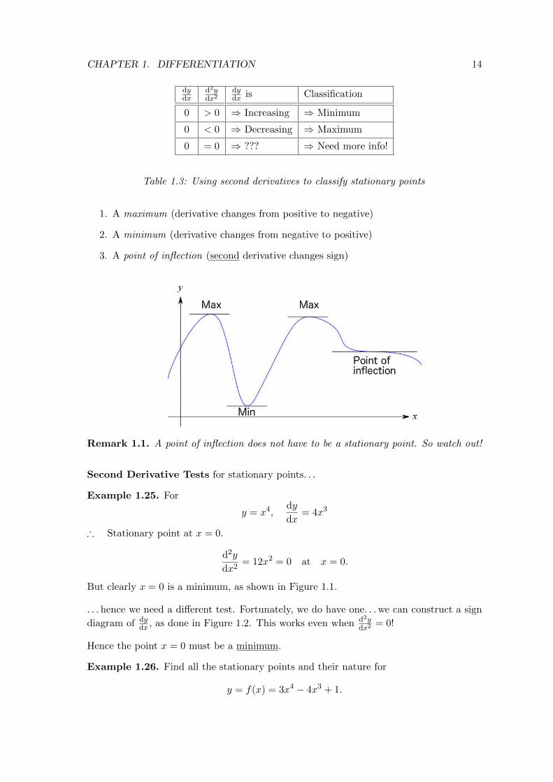
Consider the following diagram...
First observe that
1. If f ′(a) < 0 then f is decreasing near a,
2. If f ′(b) > 0 then f is increasing near b.
A stationary point is where dydx = 0. It can correspond to either. . .
CHAPTER 1. DIFFERENTIATION 14
dydx
d2ydx2
dydx is Classification
0 > 0 ⇒ Increasing ⇒ Minimum
0 < 0 ⇒ Decreasing ⇒ Maximum
0 = 0 ⇒ ??? ⇒ Need more info!
Table 1.3: Using second derivatives to classify stationary points
1. A maximum (derivative changes from positive to negative)
2. A minimum (derivative changes from negative to positive)
3. A point of inflection (second derivative changes sign)
Remark 1.1. A point of inflection does not have to be a stationary point. So watch out!
Second Derivative Tests for stationary points. . .
Example 1.25. For
y = x4,dy
dx= 4x3
∴ Stationary point at x = 0.
d2y
dx2= 12x2 = 0 at x = 0.
But clearly x = 0 is a minimum, as shown in Figure 1.1.
. . . hence we need a different test. Fortunately, we do have one. . . we can construct a sign
diagram of dydx , as done in Figure 1.2. This works even when d2y
dx2= 0!
Hence the point x = 0 must be a minimum.
Example 1.26. Find all the stationary points and their nature for
y = f(x) = 3x4 − 4x3 + 1.
CHAPTER 1. DIFFERENTIATION 15
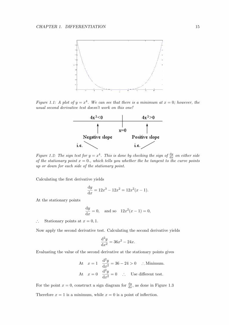
Figure 1.1: A plot of y = x4. We can see that there is a minimum at x = 0; however, theusual second derivative test doesn’t work on this one!
Figure 1.2: The sign test for y = x4. This is done by checking the sign of dydx on either side
of the stationary point x = 0., which tells you whether the he tangent to the curve pointsup or down for each side of the stationary point.
Calculating the first derivative yields
dy
dx= 12x3 − 12x2 = 12x2(x− 1).
At the stationary points
dy
dx= 0, and so 12x2(x− 1) = 0,
∴ Stationary points at x = 0, 1.
Now apply the second derivative test. Calculating the second derivative yields
d2y
dx2= 36x2 − 24x.
Evaluating the value of the second derivative at the stationary points gives
At x = 1d2y
dx2= 36− 24 > 0 ∴ Minimum.
At x = 0d2y
dx2= 0 ∴ Use different test.
For the point x = 0, construct a sign diagram for dydx , as done in Figure 1.3
Therefore x = 1 is a minimum, while x = 0 is a point of inflection.

CHAPTER 1. DIFFERENTIATION 16
Figure 1.3: Sign test for the derivative of 3x4 − 4x3 + 1, which demonstrates that x = 0has a point of inflection.
Example 1.27 (Exam Question (2007)). A curve is given by
x = t2, y = te−t. (1.2)
Find dydx and d2y
dx2.
Where does the curve have a critical (stationary) point? Is it a maximum, minimumor point of inflection? Justify your answer.
Solution: First calculate the derivatives using the chain rule...
dy
dx=
e−t − te−t
2t=
(1− t)e−t
2t
d2y
dx2=
2t[−e−t − (1− t)e−t
]− (1− t)e−t(2)
(2t)3.
= e−t−2t−��2t+ 2t2 − 2 +��2t
8t3.
=e−t
4t3(t2 − t− 1).
=e−t
4t− e−t
4t2− e−t
4t3.
Note that dydx = 0 only when t = 1 (therefore it is the only possible stationary point). For
the second derivatived2y
dx2
∣∣∣t=1
=���e−1
4−���e−1
4− e−1
4< 0,
so our stationary point is a maximum.
Don’t forget to give the Cartesian coordinates for the maximum! To do this, simplysubstitute t = 1 into Equations (1.2). You end up with:
y = 1× e−1 = e−1, x = 12 = 1,
i.e. the maximum is at (1,1
e).
1.5.2 Curve sketching
Thanks to modern technology, we can use graphics calculators (or even computers!) asa guide. However, you should work through the following recipe in order to accuratelysketch a curve.

CHAPTER 1. DIFFERENTIATION 17
First let y = f(x). Then follow this recipe:
1) Where is f defined? (Or put another way, where is it undefined?). Typically we cansometimes get vertical asymptotes.
2) Is f odd or even or neither?
3) Find where f(x) = 0 (if possible), i.e. where the curve cuts the x axis.
4) Find the value of f when x = 0, i.e. y = f(0), where the curve cuts the y axis.
5) Find ALL stationary points and their nature (and the value of f at such points)
6) Analyse the asymptotes
i. Horizontal asymptotes: What happens to y as x→ ±∞?
ii. If x = a is a vertical asymptote, what happens as x→ a+ and x→ a−?
Note: When the notation of x→ a+ is used, this refers to the right-sided limit, i.e. limx→ax>a
y.
Similarly, the notation x→ a− represents the left-sided limit limx→ax<a
y.
Note 2: Often it is possible to deduce the nature of the turning point without calculatingd2ydx2
.
Example 1.28. Sketch the curve y = f(x) = 1x2−1
.
1) Not defined at x = ±1 (i.e. vertical asymptotes as x = ±1).
2) f(−x) = f(x), therefore f(x) is even.
3) f(x) 6= 0 or all x, therefore f(x) never cuts the x-axis.
4) f(0) = −1, i.e. the curve passes through the y-axis at (0,−1)
5) For the derivative
f ′(x) = − 2x
(x2 − 1)2= 0 when x = 0,
where the nature of the turning point can be determined by analysing the verticalasymptotes; you will see that x = 0 is a maximum.
6i) For the horizontal asymptotes,
As x→∞, f(x)→∞,As x→ −∞, f(x)→∞.
6ii) For the vertical asymptotes, look at x→ 1 first.
As x→ 1+, f(x)→∞,As x→ 1−, f(x)→ −∞,

CHAPTER 1. DIFFERENTIATION 18
and similarly for x→ −1,
As x→ −1+, f(x)→ −∞,As x→ −1−, f(x)→∞.
At last! We are now in a position to sketch the curve; see Figure 1.4.
Figure 1.4: A sketch of the function y = f(x) = 1/(x2 − 1). Observe the stationary pointat x = 0; the fact that this is a maximum has been deduced with the help of the verticalasymptotes.
Example 1.29. Sketch the graph of
y2 =x(1− x)
4− x2, (1.3)
Again, we follow the recipe. . .
1) Note that
y2 =x(1− x)
(2− x)(2 + x),
therefore there are vertical asymptotes at x = ±2. Also, are only interested in real y,thus we require y2 > 0. Hence it follows that y is defined only when
x(1− x)
4− x2> 0.
The RHS of (1.3) may change sign at x = 0, 1, and possibly at the position of thevertical asymptotes! Consider the following diagram of the sign of y2:
Therefore the graph of y is undefined for
−2 ≤ x < 0 and 1 < x ≤ 2.
2) y is neither odd nor even, but observe
y = ±√x(1− x)
4− x2
and the ± sign indicated that the graph should be symmetric about the horizontal xaxis.
CHAPTER 1. DIFFERENTIATION 19
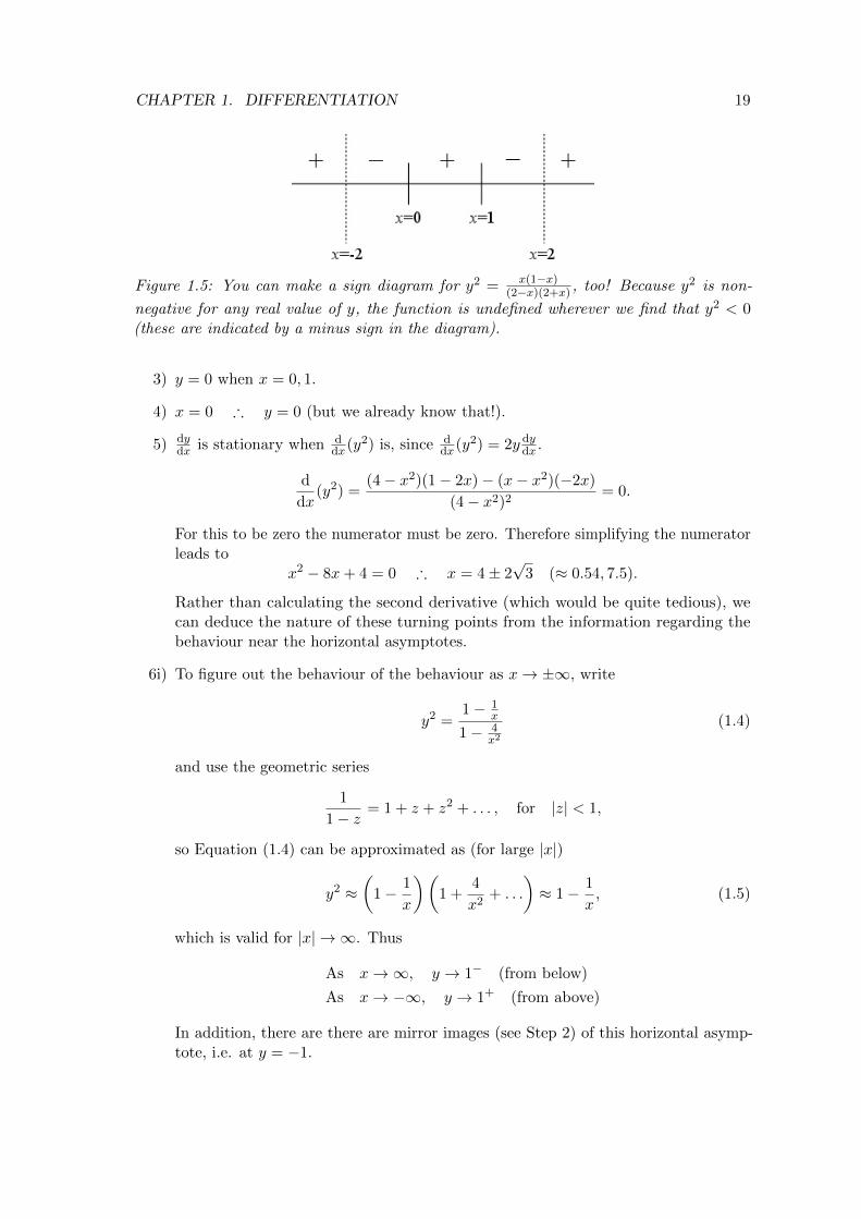
Figure 1.5: You can make a sign diagram for y2 = x(1−x)(2−x)(2+x) , too! Because y2 is non-
negative for any real value of y, the function is undefined wherever we find that y2 < 0(these are indicated by a minus sign in the diagram).
3) y = 0 when x = 0, 1.
4) x = 0 ∴ y = 0 (but we already know that!).
5) dydx is stationary when d
dx(y2) is, since ddx(y2) = 2y dy
dx .
d
dx(y2) =
(4− x2)(1− 2x)− (x− x2)(−2x)
(4− x2)2= 0.
For this to be zero the numerator must be zero. Therefore simplifying the numeratorleads to
x2 − 8x+ 4 = 0 ∴ x = 4± 2√
3 (≈ 0.54, 7.5).
Rather than calculating the second derivative (which would be quite tedious), wecan deduce the nature of these turning points from the information regarding thebehaviour near the horizontal asymptotes.
6i) To figure out the behaviour of the behaviour as x→ ±∞, write
y2 =1− 1
x
1− 4x2
(1.4)
and use the geometric series
1
1− z= 1 + z + z2 + . . . , for |z| < 1,
so Equation (1.4) can be approximated as (for large |x|)
y2 ≈(
1− 1
x
)(1 +
4
x2+ . . .
)≈ 1− 1
x, (1.5)
which is valid for |x| → ∞. Thus
As x→∞, y → 1− (from below)
As x→ −∞, y → 1+ (from above)
In addition, there are there are mirror images (see Step 2) of this horizontal asymp-tote, i.e. at y = −1.

CHAPTER 1. DIFFERENTIATION 20
Figure 1.6: Plots of the upper branch of f(x) for x < −2 and 3 < x < 9 respectively.
6ii) To get the behaviour near the vertical asymptotes it is simplest (in this case) to findwhere the curve cuts its horizontal asymptote, i.e. set y2 = 1:
∴ 4−��x2 = x−��x2 ⇒ x = 4
Hence we can sketch two parts of the upper half of the graph, see Figure 1.6.
And let’s not forget to plot the rest of the graph!
Figure 1.7: The complete sketch for the (implicit) function y2 = x(1−x)4−x2 .
1.5.3 Equations of Tangent and Normal
Example 1.30. Find equations of the tangent and normal to y = x2 at x = 1.
First find dydx , recalling that dy
dx ≡ slope of the tangent.
dy
dx= 2x, ∴
dy
dx
∣∣∣x=1
= 2.
Also, at x = 1 we have y = 1. Therefore using
y − y1 = m(x− x1)

CHAPTER 1. DIFFERENTIATION 21
where x1 = 1, y1 = 1 and m = 2, the line through (1, 1) with slope 2 has equation
y = 2x− 1.
The normal is perpendicular to the tangent. Therefore
Slope of Normal =−1
Slope of Tangent= −1
2.
The normal is the line through (1, 1) with slope = −1/2. Therefore using
y − y1 = m(x− x1)
with x1 = 1, y1 = 1 and m = −1/2 yields the equation for the normal as
y = −1
2x+
3
2.
Example 1.31. Find equations of the tangent and normal to the curve given by
y = t2, x = t3 + 1 at t = 1.
For this we use parametric differentiation
dy
dx=
dydtdxdt
=2t
3t2=
2
3at t = 1.
Also at t = 1, (x, y) = (2, 1).The tangent is the line through (2, 1) with slope 2
3 , i.e.
y − 1 =2
3(x− 2), ∴ y =
2
3x− 1
3.
The normal has slope −32 , and thus its equation is
y − 1 = −3
2(x− 2), ∴ y = −3
2x+ 4.

Chapter 2
Hyperbolic functions
2.1 Definitions of hyperbolic functions
In the first chapter, we got a few glimpses of hyperbolic functions, so now you’re probablyitching to find out just what they are. Well, that’s what this chapter is for!
First things first, here are the definitions:
sinhx =ex − e−x
2
coshx =ex + e−x
2
tanhx =ex − e−x
ex + e−x=
sinhx
coshx.
The three functions are pronounced “shine x”, “cosh x” and “tansh x” respectively.
Recall thatas x→∞, ex →∞ and e−x → 0.
1 If y = coshx = ex+e−x
2 ,cosh (0) = 1.
Also note that
y = cosh (−x) =e−x + e−(−x)
2=e−x + ex
2= coshx.
Therefore the curve is symmetrical about the y axis, i.e. is an even function.And
as x→∞, y → ex + 0
2=
1
2ex →∞.
2 If y = sinhx = ex−e−x2 ,
sinh (0) = 0.
Also,
y = sinh (−x) =e−x − e−(−x)
2=e−x − ex
2= − sinhx,
22
CHAPTER 2. HYPERBOLIC FUNCTIONS 23
therefore the curve is anti-symmetrical about the y axis, i.e. is an odd function.And
as x→∞, y → ex − 0
2=
1
2ex → +∞,
as x→ −∞, y → 0− e−x
2= −1
2e−x → −∞.
3 For
y = tanhx =ex − e−x
ex + e−x=
sinhx
coshx,
we see that
tanh (0) =0
1= 0.
Also, if we consider the limits x→ ±∞:
as x→∞, y → ex − 0
ex + 0→ 1,
as x→ −∞, y → −0− e−x
0 + e−x→ −1.
Finally, note that
tanh (−x) =sinh (−x)
cosh (−x)
=− sinhx
coshx= − tanhx,
so tanhx is an odd function.
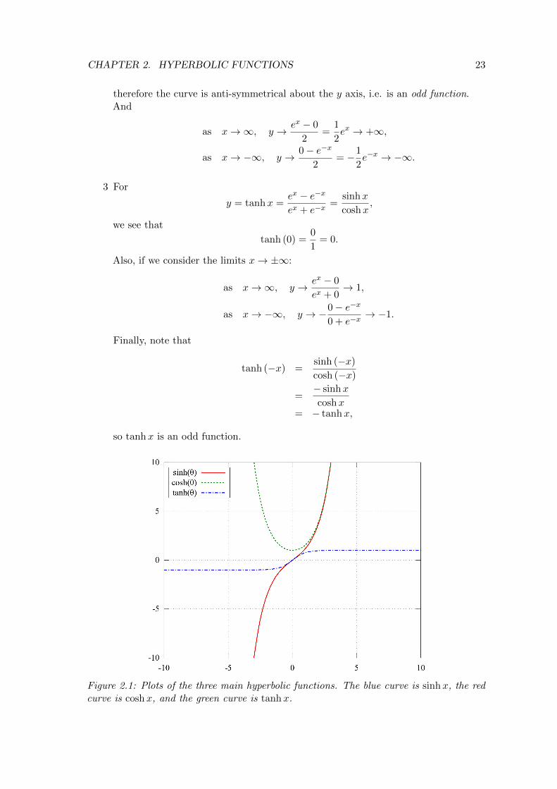
Figure 2.1: Plots of the three main hyperbolic functions. The blue curve is sinhx, the redcurve is coshx, and the green curve is tanhx.

CHAPTER 2. HYPERBOLIC FUNCTIONS 24
2.2 Inverse hyperbolic functions
The hyperbolic functions do come with inverse functions.
1 Suppose thaty = sinh−1 x, ∴ x = sinh y.
Then by definition,
x =1
2
(ey − e−y
)⇐⇒ ey − e−y = 2x
Multiplying by ey givese2y − 1− 2xey = 0,
or(ey)2 − 2x(ey)− 1 = 0,
which is a quadratic equation in ey.
∴ ey =2x±
√4x2 + 4
2
= x±√x2 + 1, .
thusey = x+
√x2 + 1, or ey = x−
√x2 + 1.
Now ey > 0 for all y, but
x−√x2 + 1 < 0,
becausex2 + 1 > x ⇒
√x2 + 1 >
√x2 = x.
So the second option (negative choice) is impossible! Hence we are left with
ey = x+√x2 + 1,
ory = sinh−1 x = ln
(x+
√x2 + 1
).
2 Suppose thaty = cosh−1 x, ⇒ x = cosh y, (so x ≥ 1).
Then by definition of cosh,
1
2
(ey + e−y
)= x ⇐⇒ ey + e−y = 2x
As before, multiply by ey to get
e2y + 1− 2xey = 0
or(ey)2 − 2x(ey) + 1 = 0.
CHAPTER 2. HYPERBOLIC FUNCTIONS 25
which is a quadratic equation in ey (again!)
∴ ey =2x±
√4x2 − 4
2
= x±√x2 − 1,
and this is real since x ≥ 1 anyway. Therefore
ey = x+√x2 − 1, or ey = x−
√x2 − 1.
Now ey > 0 for all y, and
x±√x2 − 1 > 0
are both possibilities (so we can’t rule any option out!) Observe that
1
x+√x2 − 1
=1
x+√x2 − 1
× x−√x2 − 1
x−√x2 − 1
=x−√x2 − 1
x2 − (x2 − 1)
= x−√x2 − 1.
Thus
ey = x+√x2 − 1 or ey =
1
x+√x2 − 1
.
Soy = ln
(x+
√x2 − 1
),
or
y = ln
(1
x+√x2 − 1
)= − ln
(x+
√x2 − 1
),
i.e.y = ± ln
(x+
√x2 − 1
).
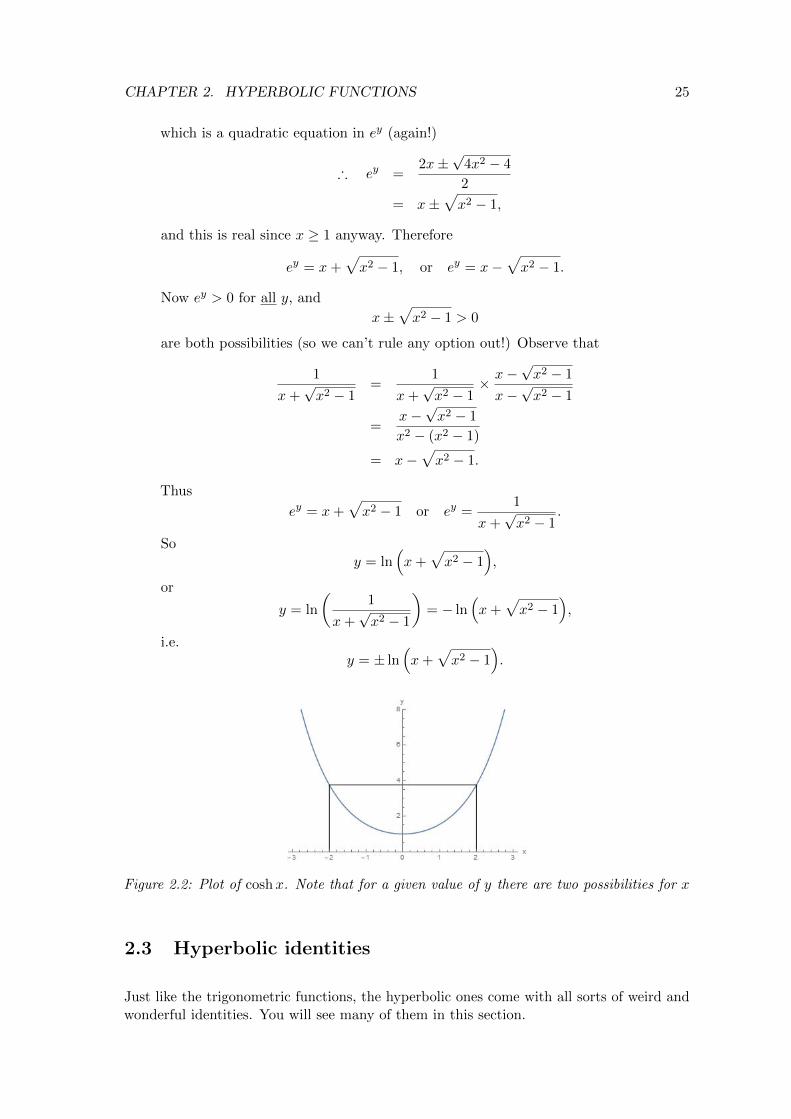
Figure 2.2: Plot of coshx. Note that for a given value of y there are two possibilities for x
2.3 Hyperbolic identities
Just like the trigonometric functions, the hyperbolic ones come with all sorts of weird andwonderful identities. You will see many of them in this section.
CHAPTER 2. HYPERBOLIC FUNCTIONS 26
Now is a good time to introduce three more hyperbolic functions. They are. . .
cothx ≡ 1tanhx
(c.f. cotx ≡ 1
tanx
)(2.1)
sechx ≡ 1coshx
(c.f. secx ≡ 1
cosx
)(2.2)
cosechx ≡ 1sinhx
(c.f. cosecx ≡ 1
sinx
)(2.3)
. . . and they are pronounced ’coth’, ’shec’ and ’coshec’ respectively.
From the definitions of sinhx and coshx,
coshx+ sinhx ≡ ex +��e−x
2+ex −��e−x
2≡ ex,
and similarly
coshx− sinhx ≡ ��ex + e−x
2−��ex − e−x
2≡ e−x,
therefore(coshx+ sinhx) (coshx− sinhx) ≡��ex��e−x ≡ 1
i.e.cosh2 x− sinh2 x ≡ 1,
which is analogous to cos2 x+ sin2 x ≡ 1.
Now divide the above result by sinh2 x to yield
cosh2 x
sinh2 x− 1 ≡ 1
sinh2 x,
∴ cosech2 x ≡ coth2 x− 1,
(which is analogous to cosec2 x ≡ cot2 x+ 1).
Recall that
coshx+ sinhx ≡ ex
coshx− sinhx ≡ e−x.
Squaring both of these yields
cosh2 x+ 2 sinhx coshx+ sinh2 x ≡ e2x (2.4)
cosh2 x− 2 sinhx coshx+ sinh2 x ≡ e2x (2.5)
and then doing (2.4) minus (2.5) yields
4 sinhx coshx ≡ e2x − e−2x ⇐⇒ 2 sinhx coshx ≡ e2x − e−2x
2,
i.e.2 sinhx coshx ≡ sinh 2x,
which is analogous to 2 sinx cosx ≡ sin 2x.
But for now, let’s just admire the Table 2.1. Notice that the hyperbolic identities arevery similar to the trigonometric counterparts, but with some different signs! This iscalled Osborne’s rule, which tells you to flip the sign whenever we have a product of sinhs;this includes cosech2 x, tanh2 x and coth2 x as well as sinh2 x! Otherwise the hyperbolicidentities are essentially the same as their trigonometric versions. You will get to deriveone of these identities as part of your homework!

CHAPTER 2. HYPERBOLIC FUNCTIONS 27
Hyperbolic Trigonometric
cothx ≡ 1/ tanhx cotx ≡ 1/ tanx
sechx ≡ 1/ coshx secx ≡ 1/ cosx
cosechx ≡ 1/ sinhx secx ≡ 1/ sinx
cosh2 x− sinh2 x ≡ 1 cos2 x+ sinx ≡ 1
sech2 x ≡ 1− tanh2 x sec2 x ≡ 1 + tan2 x
cosech2 x ≡ coth2 x− 1 cosec2 x ≡ cot2 x+ 1
sinh 2x ≡ 2 sinhx coshx sin 2x ≡ 2 sinx cosx
cosh 2x ≡ cosh2 x+ sinh2 x cos 2x ≡ cos2 x− sin2 x
cosh 2x ≡ 1 + 2 sinh2 x cos 2x ≡ 1− 2 sin2 x
cosh 2x ≡ 2 cosh2 x− 1 cos 2x ≡ 2 cos2 x− 1
Table 2.1: Lots of hyperbolic identities, along with with their trigonometric counterparts.

Chapter 3
Partial differentiation
3.1 Introduction to partial differentiation
Many quantities that we measure are functions of two or more variables.
Example 3.1. The temperature T of a rod heated suddenly from time t = 0 at one end.
Figure 3.1: The rod is heated at the end x = 0. Initially, T = 0.
Clearly T depends on:
i The distance x from the heated end
ii The time t after heating commenced.
So we writeT = T (x, t),
i.e. T is a function of the two independent variables: x and t.
Example 3.2. (More abstractly), suppose that a function f is defined as
f(x, y) = x2 + 3y2,
then the value of f is determined by every possible pair (x, y), so if (x, y) = (0, 2) then
f(0, 2) = 02 + 3× 22 = 12.
Partial derivatives generalise the derivative to functions of two or more variables.
28
CHAPTER 3. PARTIAL DIFFERENTIATION 29
Definition 3.1. Suppose f is a function of two independent variables x and y, then thepartial derivative of f(x, y) w.r.t x is defined as
∂f
∂x= fx = lim
∆x→0
f(x+ ∆x, y)− f(x, y)
∆x.
Similarly, the partial derivative of f(x, y) w.r.t y is
∂f
∂y= fy = lim
∆y→0
f(x, y + ∆y)− f(x, y)
∆y.
But. . . there’s a shortcut! If you want fx, say, then just pretend that y is a constant anddifferentiate with respect to x only. Similarly, when you want fy, simply pretend that x isconstant and go ahead with differentiating with respect to y only. And yes, this lets youuse (most) of the tricks we have from Chapter 1!
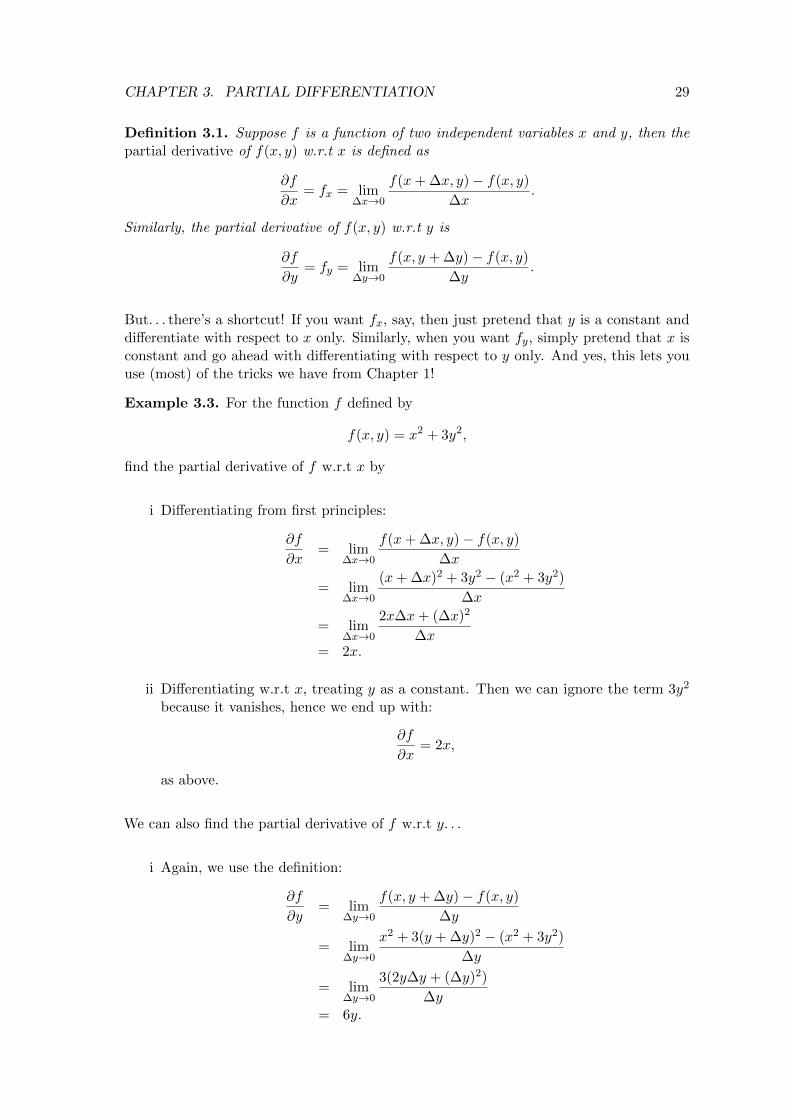
Example 3.3. For the function f defined by
f(x, y) = x2 + 3y2,
find the partial derivative of f w.r.t x by
i Differentiating from first principles:
∂f
∂x= lim
∆x→0
f(x+ ∆x, y)− f(x, y)
∆x
= lim∆x→0
(x+ ∆x)2 + 3y2 − (x2 + 3y2)
∆x
= lim∆x→0
2x∆x+ (∆x)2
∆x= 2x.
ii Differentiating w.r.t x, treating y as a constant. Then we can ignore the term 3y2
because it vanishes, hence we end up with:
∂f
∂x= 2x,
as above.
We can also find the partial derivative of f w.r.t y. . .
i Again, we use the definition:
∂f
∂y= lim
∆y→0
f(x, y + ∆y)− f(x, y)
∆y
= lim∆y→0
x2 + 3(y + ∆y)2 − (x2 + 3y2)
∆y
= lim∆y→0
3(2y∆y + (∆y)2)
∆y= 6y.

CHAPTER 3. PARTIAL DIFFERENTIATION 30
ii Alternatively, if we differentiate f w.r.t y, treating x as a constant, we see that thex2 term vanishes, leaving us with
∂f
∂y= 6y,
as expected.
Physical Interpretation: Consider the heated rod problem.
Figure 3.2: Plots showing how temperature T varies with respect to t and to x separately.
a In the top graph of Figure 3.2, ∂T∂t is the rate of change of T with time at a fixed distance x.
b In bottom graph of the same figure, ∂T∂x is the rate of change of T with distance x at
a particular instance in time.
Example 3.4. Supposef(x, y) = y sinx+ x cos2 y,
Then for the partial derivative fx
∂f
∂x= y cosx+ cos2 y
where we treated y as a constant.Meanwhile,
∂f
∂y= sinx+ 2x cos y(− sin y)
= sinx− x sin 2y
where we treated x as a constant.
Example 3.5. Suppose
f(x, y) = tan−1(yx
)then compute fx and fy.
Recall thatd
du
(tan−1 u
)=
1
1 + u2

CHAPTER 3. PARTIAL DIFFERENTIATION 31
Therefore, calculating fx (treating y as a constant):
fx =1
1 +( yx
)2 ∂
∂x
(yx
)=
1
1 +( yx
)2 (− y
x2
),
i.e∂f
∂x= fx = − y
x2 + y2.
Similarly, calculating fy (treating x as a constant):
fy =1
1 +( yx
)2 ∂
∂y
(yx
)=
1
1 +( yx
)2 (1
x
),
i.e∂f
∂y= fy =
x
x2 + y2.
Example 3.6 (Exam Question 2008). If a function f(x, y) is defined as
f(x, y) = x ln
(x
y
),
then find ∂f∂x and ∂f
∂y .
Solution: Note that
f(x, y) = x ln
(x
y
)= x (lnx− ln y) ,
so for the x derivative,
∂f
∂x= 1 · (lnx− ln y) + x
(1
x− 0
)= (lnx− ln y) +�x ·
1
�x
= lnx− ln y + 1
= ln
(x
y
)+ 1.
Meanwhile, for the y derivative
∂f
∂y= 0− ∂
∂y(x ln y)
= −x ∂∂y
(ln y)
= −xy.
Example 3.7 (Function with three variables). Suppose f(x, y, z) is defined as
f(x, y, z) = zey cosx
then
∂f
∂x= −zey sinx,
∂f
∂y= zey cosx,
∂f
∂y= ey cosx.
CHAPTER 3. PARTIAL DIFFERENTIATION 32
3.2 Higher Partial Derivatives
You can differentiate the first partial derivatives again to obtain second partial derivatives.
fxx =∂
∂x
(∂f
∂x
)=∂2f
∂x2
fyy =∂
∂y
(∂f
∂y
)=∂2f
∂y2
fxy =∂
∂y
(∂f
∂x
)=
∂2f
∂y∂x
fyx =∂
∂x
(∂f
∂y
)=
∂2f
∂x∂y
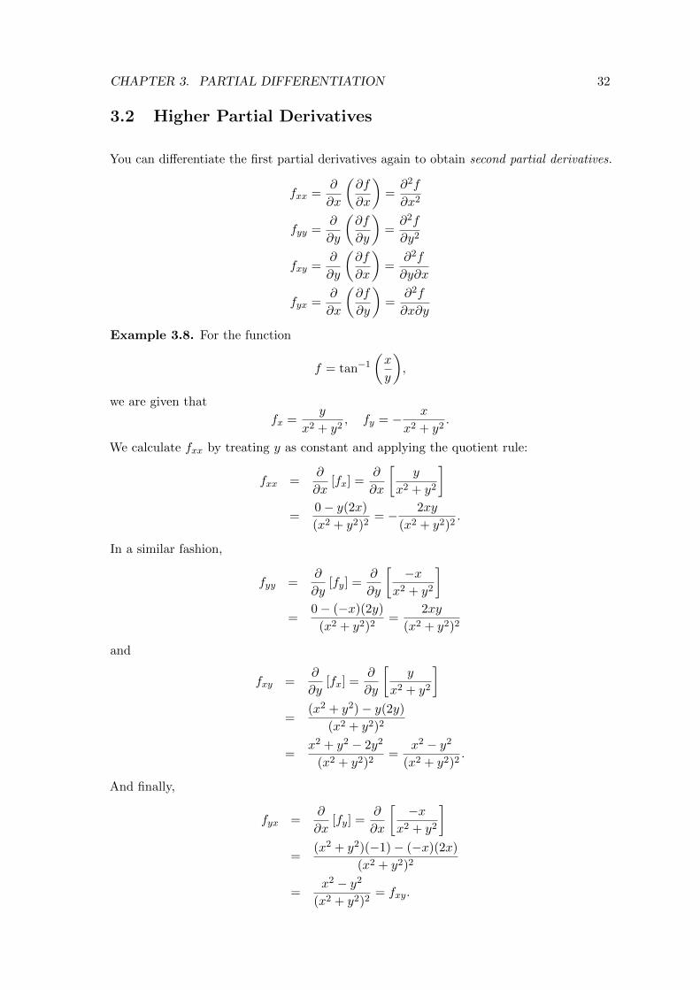
Example 3.8. For the function
f = tan−1
(x
y
),
we are given that
fx =y
x2 + y2, fy = − x
x2 + y2.
We calculate fxx by treating y as constant and applying the quotient rule:
fxx =∂
∂x[fx] =
∂
∂x
[y
x2 + y2
]=
0− y(2x)
(x2 + y2)2= − 2xy
(x2 + y2)2.
In a similar fashion,
fyy =∂
∂y[fy] =
∂
∂y
[−x
x2 + y2
]=
0− (−x)(2y)
(x2 + y2)2=
2xy
(x2 + y2)2
and
fxy =∂
∂y[fx] =
∂
∂y
[y
x2 + y2
]=
(x2 + y2)− y(2y)
(x2 + y2)2
=x2 + y2 − 2y2
(x2 + y2)2=
x2 − y2
(x2 + y2)2.
And finally,
fyx =∂
∂x[fy] =
∂
∂x
[−x
x2 + y2
]=
(x2 + y2)(−1)− (−x)(2x)
(x2 + y2)2
=x2 − y2
(x2 + y2)2= fxy.

CHAPTER 3. PARTIAL DIFFERENTIATION 33
Fact: If fx, fy, fxy and fyx are continuous (i.e. doesn’t ’jump’) at (x, y), then fxy = fyx,i.e. fyx = fxy holds for any f .
Example 3.9. Letf(x, y) = xe2y.
fx = e2y fy = 2xe2y fy = 2xe2y
fxy = 2e2y fyx = 2e2y fyy = 4xe2y
fxyy = 4e2y fyxy = 4e2y fyyx = 4e2y
i.e.fxyy = fyxy = fyyx
so the order does not matter.
Example 3.10 (Exam Question 2004). a) Verify that f(x, y) = e−(1+a2)x cos ay is asolution of the equation
∂f
∂x=∂2f
∂y2− f.
Solution: First compute the required derivatives
∂f
∂x= −(1 + a2)e−(1+a2)x cos ay
∂f
∂y= −ae−(1+a2)x sin ay
∂2f
∂y2= −a2e−(1+a2)x cos ay
So computing the RHS (right hand side)
RHS = fyy − f= −a2e−(1+a2)x cos ay − e−(1+a2)x cos ay
= −(1 + a2)e−(1+a2)x cos ay = LHS.
b Let g = yf(xy). Show that
y∂g
∂y− x∂g
∂x= g.
Solution:
∂g
∂y= = f(xy) + yxf ′(xy),
∂g
∂x= y2f ′(xy),
where primes denote differentiation w.r.t the combined variable xy.
Note: To see this, considerd
dx(sin 2x) = 2 cos 2x,
CHAPTER 3. PARTIAL DIFFERENTIATION 34
i.ed
dx(f(2x)) = 2f ′(2x).
Also consider∂
∂x(sinxy) = y cosxy,
and therefore∂
∂x(f(xy)) = yf ′(xy).
Hence returning to the example,
LHS = yf(xy) +�����xy2f ′(xy)−���
��xy2f ′(xy) = g(x, y) = RHS,
as required.

Chapter 4
Integration
4.1 The basics
There are two ways to interpret integration. . .
1. Integration is the reverse of differentiation! If we have, say,
dA(x)
dx= f(x),
then we can write
A(x) =
∫f(x)dx+ C. [Indefinite integral!]
We say that A is the integral (antiderivative) of f(x).
2. Integration gives the area under a curve To achieve this, you sum the contri-bution of lots of infinitesimally small pieces.
To demonstrate, consider the area bounded by the x-axis, the lines x = a, x = b andthe curve y = f(x), as shown in the following diagram:
It is often taken for granted that the two interpretations are the same. In fact, thisis not obvious, so mathematicians have a big theorem about it. . .
35

CHAPTER 4. INTEGRATION 36
Theorem: Fundamental Theorem of CalculusThe shaded area above is ∫ b
af(x)dx.
Proof: Let A(x) = area from say, the origin O to the point x under the curve. Thenthe area of the shaded rectangle is
A(x+ h)−A ≈ f(x)h.
[Note: The intuition behind the above approximation is that it becomes moreaccurate as h→ 0!]
∴ f(x) ≈ A(x+ h)−A(x)
h→ dA(x)
dxas h→ 0.
Therefore the area from x = a to x = b is
A(b)−A(a) =
∫ b
af(x)dx. [A number; a definite integral!]
�
When tackling an integral, an engineer can count on these standard results. . .
f(x)∫f(x)dx
xn (n 6= −1) 1n+1x
n+1 + C
x−1 ln |x|+ C
eax 1aeax + C
cos (ax) 1a sin (ax) + C
sin (ax) − 1a cos (ax) + C
1x2+1
tan−1 x+ C
Table 4.1: Table of Basic Integrals
CHAPTER 4. INTEGRATION 37
4.2 Integration by substitution
Sometimes an integral is easier to solve if you change the variable you are integrating withrespect to, i.e. make a substitution.
Formally, if I =
∫ x2
x1
f(x) dx,
try introducing u = g(x),
⇒ du
dx= g′(x) or
dx
du=
1
g′(x),
so we end up with something that looks like multiplying and dividing by du:
I =
∫ x2
x1
f(x) dx =
∫ u2
u1
f(u)dx
dudu,
where u1 = g(x1), u2 = g(x2). So you must change the upper and lower limits for yourdefinite integral.
The best time to use this is when you have a function “wrapped” in another function youwould like to unravel.
Example 4.1. Calculate the integral∫(3x− 7)−5dx.
We want to remove the “function of a function”, so let
u = 3x− 7 ⇒ du = 3dx ⇒ dx =1
3du,
then ∫(3x− 7)−5dx =
1
3
∫u−5du
=1
3
(−1
4u−4
)+ C
= − 1
12u−4 + C
= − 1
12(3x− 7)−4 + C.
Don’t forget to rewrite your final answer in terms of x!
Example 4.2. Calculate the integral ∫sin√x√
xdx.
Here, the ’horrible’ bit is√x, so let
u =√x ⇒ du =
1
2√x
dx,

CHAPTER 4. INTEGRATION 38
i.e.dx = 2
√xdu = 2udu∫
sin√x√
xdx =
∫sinu
�u.2�udu
= 2
∫sinudu
= −2 cosu+ C
= −2 cos√x+ C.
Example 4.3.
I =
∫ √x(1 +√x) 1
4 dx.
If we let u =√x we still end up with a term that looks like u2(1+u)
14 which is still difficult
to deal with.
How about. . .u = 1 +√x?
du =1
2√x
dx ⇒ dx = 2√xdu = 2(u− 1) = 2
√xdu.
Subsequently,∫ √x(1 +√x) 1
4 dx =
∫(u− 1)u
14 2(u− 1)du
= 2
∫(u− 1)2u
14 du
= 2
∫u
14(u2 − 2u+ 1
)du
= 2
(4
13u
134 − 2
4
9u
94 +
4
5u
54
)+ C
=8
13(1 +
√x)
134 − 16
9(1 +
√x)
94 +
8
5(1 +
√x)
54 + C.
4.2.1 A question of logs
Let us consider the derivative of the logarithm of some general function f(x):
d
dx(ln(f(x))) =
1
f(x)· d
dx(f(x))
=f ′(x)
f(x)
This implies that: ∫f ′(x)
f(x)dx = ln(f(x)) + c
Example 4.4. Consider the the following integral:
I =
∫2x+ 5
x2 + 5x+ 3dx
CHAPTER 4. INTEGRATION 39
Now, if we choose f(x) = x2 + 5x+ 3, then f ′(x) = 2x+ 5. So, if we differentiate ln(f(x)),in this case we have
d
dx
[ln(x2 + 5x+ 3)
]=
2x+ 5
x2 + 5x+ 3,
by the chain rule. Thus we know the integral must be
I = ln(x2 + 5x+ 3) + C.
4.2.2 Trigonometric and hyperbolic substitutions
If you see Try substituting√a2 − x2 x = a sin θ√a2 + x2 x = a sinh θ√x2 − a2 x = a cosh θ
1
a2 + x2x = a tan θ
Example 4.5 (To show why).
I =
∫1√
a2 + x2dx.
If we let x = a sinh θ, thendx = a cosh θdθ,
thus
I =
∫a cosh θ√
a2 + a2 sinh2 θdθ
=
∫�a cosh θ
�a√
1 + sinh2 θdθ
=
∫cosh θ
cosh θdθ
=
∫1dθ
= θ + C = sinh−1(xa
).
Example 4.6 (Harder!).
I =
∫ −1
−3
1√14− 12x− 2x2
dx
=1√2
∫ −1
−3
1√7− 6x− x2
dx,
Not obvious what the next step is.
Complete the square in the denominator!
7− 6x− x2 = 7− (x+ 3)2 + 9 = 16− (x+ 3)2.
CHAPTER 4. INTEGRATION 40
Hence
I =1√2
∫ −1
−3
1√16− (x+ 3)2
dx,
which looks like1√
a2 − u2,
so we will choose a substitution like a sin θ.
Let u = x+ 3, then du = dx, and as a result:
I =1√2
∫ 2
0
1√16− u2
du.
Now putu = 4 sin θ ⇒ du = 4 cos θdθ.
I =1√2
∫ π6
0
4 cos θ√16− 16 sin2 θ
dθ
=1√2
∫ π6
0
����4 cos θ
����4 cos θ
dθ
=1√2
∫ π6
01dθ
=π
6√
2
=π√
2
12.
4.2.3 One more trick
If you see an integral like ∫sin4 x cosxdx,
try u = sinx, because you get du = cosxdx, making the cos term disappear.
However, if you are facing ∫sin4 x cos3 xdx,
keep your eyes open for less obvious clues!
=
∫sin4 x cos2 x cosxdx
=
∫sin4 x(1− sin2 x) cosxdx
=
∫sin4 x cosxdx−
∫sin6 x cosxdx,
then we can summon u = sinx.

CHAPTER 4. INTEGRATION 41
Remark 4.1. This even works for, say,∫cos5 xdx =
∫(1− sin2 x)2 cosxdx
And finally. . . be bold! Try!
4.3 Integration by parts
This is a good strategy when you are integrating a product of two terms, one of whicheither differentiates or integrates into something simpler.
Recall the product rule:d
dx(uv) = v
du
dx+ u
dv
dx
Now integrate both sides w.r.t. x:
uv =
∫v
du
dxdx+
∫u
dv
dxdx
⇒∫u
dv
dxdx = uv −
∫v
du
dxdx︸ ︷︷ ︸
Another integral!
,
The idea is that u becomes “better” as you differentiate ordv
dxbecomes “better” as you
integrate.
Example 4.7. Find ∫xexdx.
Since x differentiates away nicely,
choose u = x,dv
dx= ex,
thendu
dx= 1, v =
∫exdx = ex.
Apply the by parts formula: ∫xexdx = xex −
∫1 · exdx
= xex − ex + C.
= ex(x− 1) + C.
(4.1)
(Note that the arbitrary constant has been included right at the very last step)
Question: What happens if you try the other way round?
If u = ex,dv
dx= x,

CHAPTER 4. INTEGRATION 42
thendu
dx= ex, v =
x2
2,
which already does not look promising. If we go ahead and use the by-parts rule, then. . .∫xexdx =
x2
2ex − 1
2
∫x2exdx,
which is true, but does not help!
So what have we learned from this example? Well, it does matter which term you choose
for u ordv
dx, as it can make or break your hopes of solving an integral. So choose wisely!
Example 4.8. Find
I =
∫e2x sinxdx.
Let
u = sinx,dv
dx= e2x,
thendu
dx= cosx, v =
1
2e2x
and the by-parts formula gives:
I =1
2e2x sinx− 1
2
∫e2x cosxdx
=1
2e2x sinx− 1
2J ,
where
J =
∫e2x cosxdx,
yet another integral. But don’t panic! This one can be handled by parts too; simply let
u = cosx,dv
dx= e2x,
thendu
dx= − sinx, v =
1
2e2x,
which gives
J =1
2e2x cosx+
1
2
∫e2x sinxdx
=1
2e2x cosx+
1
2I .
∴ I =1
2e2x sinx− 1
4
(e2x cosx+ I
)⇒ 5
4I =
1
2e2x sinx− 1
4e2x cosx,
So, finally, we have:
∴ I =1
5
(2e2x sinx− e2x cosx
)+ C,
not forgetting the constant of integration at the very end!
CHAPTER 4. INTEGRATION 43
Example 4.9. Compute∫lnx dx. (Classic A-Level question!)
∫lnx dx =
∫1 · lnxdx
= x lnx−∫�x
1
�xdx
= x(lnx− 1) + C.
Example 4.10. Find
I =
∫sin−1 x dx.
I =
∫1 · sin−1 xdx
= x sin−1 x−∫
x√1− x2
dx
= x sin−1 x−√
1− x2.
4.4 Using partial fractions
Sometimes we want to compute, say,∫x+ 1
x2 − 3x+ 2dx,
which we can’t integrate directly. Here we must express the integrand as a sum of partialfractions.
4.4.1 Recap: Partial fractions
You can express the functionP (x)
Q(x)with partial fractions if Q(x) factorises.
For every factor of Q(x) You get this partial fraction form:
(ax+ b)A
(ax+ b)
(ax+ b)2 A
(ax+ b)+
B
(ax+ b)2
(ax+ b)3 A
(ax+ b)+
B
(ax+ b)2+
C
(ax+ b)3
(ax2 + bx+ c)Ax+B
ax2 + bx+ c
Then plug in some different values of x to find A, B, . . . (or use any other method youprefer!)
For the next three examples P (x) will be linear and Q(x) will be quadratic polynomials.
CHAPTER 4. INTEGRATION 44
Example 4.11 (Case 1: Denominator has two real roots).∫3x− 5
x2 − 2x− 3dx.
First things first. . . factorise the denominator!
x2 − 2x− 3 ≡ (x− 3)(x+ 1)
∴3x− 5
x2 − 2x− 3≡ A
(x− 3)+
B
x+ 1.
Hence3x− 5 ≡ A(x+ 1) +B(x− 3).
Let’s try two different values of x. How about. . . ?
x = −1⇒ −8 = −4B ⇒ B = 2,
x = 3⇒ 4 = 4A⇒ A = 1,
∴3x− 5
x2 − 2x− 3≡ 1
(x− 3)+
2
x+ 1.
Then ∫3x− 5
x2 − 2x− 3dx
=
∫ (1
x− 3+
2
x+ 1
)dx
=
∫1
x− 3dx+
∫2
x+ 1dx
= ln |x− 3|+ 2 ln |x+ 1|+ C.
Example 4.12 (Case 2: Denominator has one real root).∫x
x2 − 2x+ 1dx.
Start withx
x2 − 2x+ 1≡ x
(x− 1)2≡ A
x− 1+
B
(x− 1)2.
∴ x ≡ A(x− 1) +B ≡ Ax+B −A.
Let’s compare coefficients: the x terms suggest that A = 1. As for the constant terms:
B −A = 0⇒ A = B = 1.
Therefore ∫x
x2 − 2x+ 1dx
=
∫1
x− 1dx+
∫1
(x− 1)2dx
= ln |x− 1| − 1
x− 1+ C.

CHAPTER 4. INTEGRATION 45
Example 4.13 (Case 3: Denominator has no real roots).∫x− 2
x2 − 2x+ 5dx
So we can’t factorise the denominator, but we can still complete the square!
x2 − 2x+ 5 = (x− 1)2 + 4,
thus the integral is ∫x− 2
(x− 1)2 + 4dx.
Looks like something with (u2 + 1), so choose
x− 1 = u, ⇒ dx = du.
Then ∫x− 2
x2 − 2x+ 5dx =
∫u− 1
u2 + 4du
=
∫u
u2 + 4du−
∫1
u2 + 4du.
Now ∫u
u2 + 4du =
1
2ln |u2 + 4|
=1
2ln |(x− 1)2 + 4|,
while for the other u-integral, try
u = 2 tan θ ⇒ du = 2 sec2 θdθ,
hence ∫1
u2 + 4du =
∫2 sec2 θ
4 tan2 θ + 4dθ
=
∫���sec2 θ
2���
sec2 θdθ
=
∫1
2dθ
=1
2θ + C =
1
2tan−1
(x− 1
2
)+ C.
Thus our final answer is∫x− 2
x2 − 2x+ 5dx =
1
2ln(x2 − 2x+ 5
)+
1
2tan−1
(x− 1
2
)+ C.
Remark 4.2. If degree ofP ≥ degree ofQ, use long division first to get N(x) +R(x)
Q(x)(R
for remainder!). Then use partial fractions onR(x)
Q(x).

CHAPTER 4. INTEGRATION 46
Example 4.14. Evaluate the indefinite integral∫x3 + 2x
x− 1dx
Do the long division first:
x2 + x+ 3
x− 1)
x3 + 2x− x3 + x2
x2 + 2x− x2 + x
3x− 3x+ 3
3
∴∫x3 + 2x
x− 1dx =
∫ (x2 + x+ 3 +
3
x− 1
)dx
=x3
3+x2
2+ 3x+ 3 log |x− 1|+ C.
4.5 Some trigonometric integrals
i Evaluate ∫cos2 xdx =
∫1
2(cos 2x+ 1) dx
=1
4sin 2x+
1
2x+ C.
ii Evaluate ∫sin2 xdx =
∫1
2(1− cos 2x)dx
=1
2x− 1
4sin 2x+ C.
4.6 Using integration
As stated at the start of the chapter, integration is great for calculating areas under curves.
Example 4.15 (1997 Exam question). Sketch the region enclosed by the curve y =1
1 + x2
and the line y =1
2and find its area.
Apply the recipe for curve sketching:

CHAPTER 4. INTEGRATION 47
• No vertical asymptotes
• An even function
• Passes through (0, 1)
• y 6= 0, and in fact y > 0 for all x.
• y → 0 as x→ ±∞.
• For the turning points
dy
dx= − 2x
(1 + x2)2= 0 when x = 0.
Now don’t forget the sketch!
Figure 4.1: A sketch of the curve y =1
1 + x2(red) and the line y =
1
2(yellow). The
enclosed region is shaded in green.
A =
∫ 1
−1
1
1 + x2dx− (Area of Rectangle)
=
∫ 1
−1
1
1 + x2dx− 2× 1
2
=[tan−1 x
]1−1− 1
=π
4−(−π
4
)− 1 =
π
2− 1.
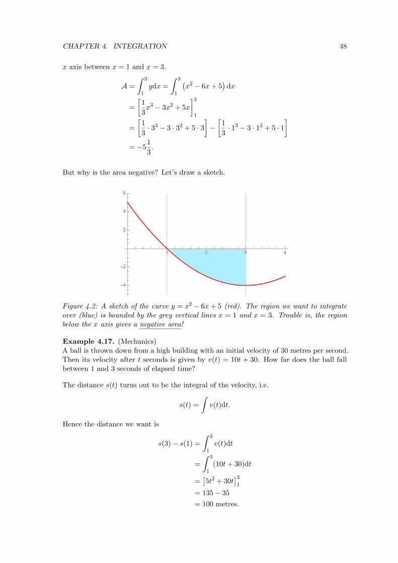
Example 4.16. Question: Find the area bounded by the curve y = x2 − 6x+ 5 and the
CHAPTER 4. INTEGRATION 48
x axis between x = 1 and x = 3.
A =
∫ 3
1ydx =
∫ 3
1
(x2 − 6x+ 5
)dx
=
[1
3x3 − 3x2 + 5x
]3
1
=
[1
3· 33 − 3 · 32 + 5 · 3
]−[
1
3· 13 − 3 · 12 + 5 · 1
]= −5
1
3.
But why is the area negative? Let’s draw a sketch.
Figure 4.2: A sketch of the curve y = x2 − 6x+ 5 (red). The region we want to integrateover (blue) is bounded by the grey vertical lines x = 1 and x = 3. Trouble is, the regionbelow the x axis gives a negative area!
Example 4.17. (Mechanics)A ball is thrown down from a high building with an initial velocity of 30 metres per second.Then its velocity after t seconds is given by v(t) = 10t + 30. How far does the ball fallbetween 1 and 3 seconds of elapsed time?
The distance s(t) turns out to be the integral of the velocity, i.e.
s(t) =
∫v(t)dt.
Hence the distance we want is
s(3)− s(1) =
∫ 3
1v(t)dt
=
∫ 3
1(10t+ 30)dt
=[5t2 + 30t
]31
= 135− 35
= 100 metres.

CHAPTER 4. INTEGRATION 49
Example 4.18. Find the area A of an ellipse, given by the equation
x2
a2+y2
b2= 1,
Figure 4.3: An ellipse
Note from Figure 4.3 that A = 4×A1 by symmetry. Hence for the area A,
A = 4
∫ a
0b
√1− x2
a2dx
= 4b
∫ a
0
√1− x2
a2dx,
an integral that can be solved by substitution. Let
x
a= sinu, ⇒ dx
du= a cosu
and √1− x2
a2=√
1− sin2 u = cosu.
So we have
A = 4b
∫ u2
u1
cosu(a cosu) du.
Reminder: In changing the variable it is also very important to change the limits, i.e.find numerical values for u1 and u2.
When x = a, sinu = 1, ∴ u =π
2.
When x = 0, sinu = 0, ∴ u = 0.
Therefore we have
A = 4ab
∫ π2
0cos2 udu

CHAPTER 4. INTEGRATION 50
Proceeding with the integral, we get
A = 4ab
∫ π2
0cos2 udu
= 4ab
∫ π2
0
(1
2+
1
2cos 2u
)du
= 4ab
(1
2u+
1
4sin 2u
)= 4ab
(π4
+ 0− (0 + 0))
= πab.
Note: For a circle, a = b which givws A = πa2.
4.7 Improper integrals
Often, you will come across integrals of the type∫ ∞a
f(x)dx.
This is an improper integral, and it must be interpreted as
= limb→∞
∫ b
af(x)dx,
if the limit exists! (If it doesn’t, the integral is said to diverge).
Remark 4.3. Technically, there are other kinds of improper integrals, in which
I =
∫ b
af(x)dx
has a problem because f(x) “blows up” at a, b or some point c in between (a < c < b). Butwe won’t worry about them here!
Example 4.19. Consider
I =
∫ ∞1
1
xndx, n > 1.
Then ∫ ∞1
1
xndx = lim
b→∞
∫ b
1
1
xndx
= limb→∞
(1
n− 1
[1− 1
bn−1
])=
1
n− 1
Remark 4.4. This integral in this last example diverges for n ≤ −1.

Chapter 5
Differential Equations
5.1 Introduction
Many problems in engineering and physical science (also biology, economics, etc.) can bereduced to solving differential equations.
Example 5.1 (RLC Series Circuit). Consider the following series circuit comprised of aresistor, a capacitor and an inductor. This circuit is known as an RLC circuit.
Figure 5.1: An RLC Circuit
Ld2I
dt2+R
dI
dt+
1
CI = E (5.1)
where
I ≡ Current Flowing in a Circuit
C ≡ Capacitance
R ≡ Resistance
L ≡ Inductance
E ≡ Voltage.
where C,R,L and E are constants and I is the unknown function to be found.
51
CHAPTER 5. DIFFERENTIAL EQUATIONS 52
An ordinary differential equation (ODE) is a relation between a function y(x), x, and the
derivativesdy
dx,
d2y
dx2, etc.
The order of the ODE is the order of the highest derivative in the equation.
An ODE is linear if there are no products of y and its derivatives, e.g.
ydy
dx, y2
and no functions of y and its derivatives, such as
ey, cos y.
For example, Equation (5.1) is a linear second order ode.
Example 5.2 (Legendre’s Equation).
(1− x2)y′′ − 2xy
′+ k2y = 0 (k = constant)
is ubiquitous in problems with spherical symmetry (e.g a Hydrogen atom). It is a linearsecond order equation.
Example 5.3 (Radioactive decay).
dR
dt= −kR. (k = constant)
This is first order and linear.
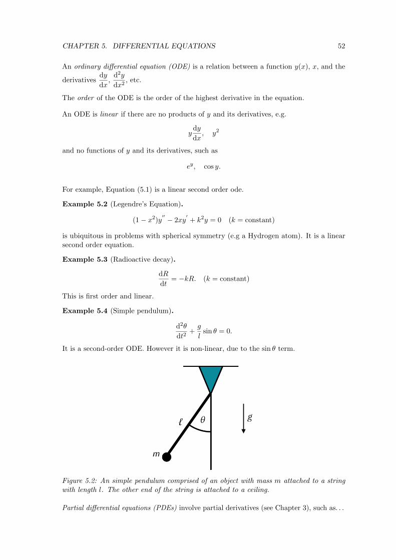
Example 5.4 (Simple pendulum).
d2θ
dt2+g
lsin θ = 0.
It is a second-order ODE. However it is non-linear, due to the sin θ term.
Figure 5.2: An simple pendulum comprised of an object with mass m attached to a stringwith length l. The other end of the string is attached to a ceiling.
Partial differential equations (PDEs) involve partial derivatives (see Chapter 3), such as. . .
CHAPTER 5. DIFFERENTIAL EQUATIONS 53
Example 5.5 (Beam Equation). The Beam Equation provides a model for the loadcarrying and deflection properties of beams, and is given by
∂2u
∂t2+ c2∂
4u
∂x4= 0.
. . . but you won’t see them in this course. You’ll have to wait until Maths for Engineers 3(MATH6503) for that!
5.2 First order separable ODEs
An ODEdy
dx= F (x, y) is separable if we can write F (x, y) = f(x)g(y) for some functions
f(x), g(y).
Example 5.6.dy
dx= y IS separable,
dy
dx= x2 − y2 IS NOT.
Example 5.7. Find the general solution to the ODE
9ydy
dx+ 4x = 0.
“Separating the variables”, we have
9ydy = −4xdx ⇐⇒
9
∫ydy = −4
∫xdx
9
2y2 = −4
2x2 + C,
i.e. the general solution is
x2
9+y2
4= K, (K = C/36)
which describes a ‘family’ of ellipses.
We can check our solution by differentiating:
2
9x+
2
4yy′
= 0
i.e9yy
′+ 4x = 0.
Example 5.8. Find the general solution to
dy
dx=y + 1
x+ 1.

CHAPTER 5. DIFFERENTIAL EQUATIONS 54
⇒∫
1
y + 1dy =
∫1
x+ 1dx
⇒ ln |y + 1| = ln |x+ 1|+ C.
Use log(ab
)= log a− log b:
ln
∣∣∣∣y + 1
x+ 1
∣∣∣∣ = C,
ory + 1
x+ 1= eC = K.
Again we can easily check this using differentiation.
Example 5.9. Solve the ODEdy
dx= 1 + y2
Separating variables: ∫dy
1 + y2=
∫dx
⇒ arctan y = x+ C
⇒ y = tan (x+ C).
Once again, this is easily checked by differentiation.
Example 5.10 (2007 Exam Question). Solve
dy
dx− y(y + 1)
x(x− 1)= 0
finding y explicitly, i.e y = f(x).
Solution: This equation is separable, thus separating the variables and integrating gives
dy
dx=y(y + 1)
x(x− 1)∫dy
y(y + 1)=
∫dx
x(x− 1).
To solve the integrals, use partial fractions:∫ [1
y− 1
y + 1
]dy =
∫ [−1
x+
1
x− 1
]dx
ln y − ln (y + 1) = − lnx+ ln (x− 1) + C
ln
(y
y + 1
)= ln
(x− 1
x
)+ C
y + 1
y= e−C
x
x− 1.
Let K = eC . Then
y = (y + 1)
(x− 1
Kx
)y
[1−
(x− 1
Kx
)]=
(x− 1
Kx
)y(Kx− x+ 1) = x− 1.

CHAPTER 5. DIFFERENTIAL EQUATIONS 55
∴ y =x− 1
Kx− x+ 1
is the explicit solution.
Example 5.11 (2010 Exam Question). Solve
(y + x2y)dy
dx= 1.
Solution:
y(1 + x2)dy
dx= 1∫
y dy =
∫dx
x2 + 1
y2
2= arctanx+ C
i.e. the solution is y = ±√
2 arctanx+ 2C.
5.3 First order linear ODEs
Aside: Exact types An exact type is where the LHS of the differential equation is theexact derivative of the product.
Example 5.12.
xdy
dx+ y = ex
⇒ d
dx(xy) = ex
⇒ xy = ex + C.
Example 5.13.
exeydy
dx+ exey = e2x
⇒ d
dx(exey) = e2x
⇒ exey =1
2e2x + C.
I recommend that you bear this in mind as we proceed. . .
First order linear ODEs are equations that may be written in the form:
dy
dx+ P (x)y = Q(x). (5.2)
Example 5.14.
dy
dx+ y cotx = cosecx. [P (x) = cotx, Q(x) = cosecx]
CHAPTER 5. DIFFERENTIAL EQUATIONS 56
Example 5.15.
tanxdy
dx+ y = ex tanx
⇒ dy
dx+ cotx y = ex. [P (x) = cotx, Q(x) = ex]
In general, Equation (5.2) is NOT exact.
Big question: Can we multiply the equation by a function of x which will make itexact?
Let’s suppose we can, and call this function I(x); the integrating factor (IF). Thenmultiply both sides of (5.2) by I:
Idy
dx+ IPy︸ ︷︷ ︸
Exact type
= IQ.
Compare the LHS withddx
(Iy)︷ ︸︸ ︷I
dy
dx+
dI
dxy,
Hence we require
IP �y =dI
dx �y
⇒ dI
dx= IP
⇒∫
dI
I=
∫P dx
⇒ ln I =
∫P dx [No need for integration constants!]
⇒ ln I = e∫P dx,
and this is the IF. We will substitute this into (5.2):
dy
dx+ P (x)y = Q(x).
Multiply by I:
e∫P dx dy
dx+ e
∫P dxPy = e
∫P dxQ
⇒ d
dx(ye
∫P dx) = e
∫P dxQ
⇒ yI =
∫e∫P dxQdx.
This is the form we end up with.
I will not ask you to go through this derivation in the exam. However, you will need toknow how to apply it.

CHAPTER 5. DIFFERENTIAL EQUATIONS 57
Example 5.16. Solvedy
dx+ 2y = e−x.
We require the IF:I = e
∫P dx = e
∫2 dx = e2x.
Then
e2x dy
dx+ 2e2xy = e2xe−x
⇒ d
dx(ye2x) = ex
⇒ ye2x = ex + C,
ory = e−x + Ce−2x.
Example 5.17. Solve
cosxdy
dx+ y sinx =
1
2sin 2x.
Get it into the right form first!
⇒ dy
dx+ y tanx =
sin 2x
2 cosx=�2 sinx���cosx
�2���cosx
⇒ dy
dx+ y tanx = sinx, (5.3)
so P (x) = tanx. Now seek the IF:
I = e∫P dx = e
∫tanxdx = e− ln(cosx) =
1
eln(cosx)=
1
cosx.
A VERY common error: e− ln(cosx) = cosx.
Multiply (5.3) throughout by I to give
1
cosx
dy
dx+
tanx
cosxy = tanx,
i.e.
d
dx
( y
cosx
)= tanx
⇒ y
cosx=
∫tanx dx+ C = − ln(cosx) + C.
Therefore the general solution is
y = C cosx− cosx ln(cosx).
Example 5.18. Solve
xdy
dx+ = x2 + 3y.
Get it in the right form first. . .dy
dx− 3
xy = x. (5.4)

CHAPTER 5. DIFFERENTIAL EQUATIONS 58
Find the integrating factor
I(x) = e∫− 3x
dx = e−3 lnx = eln(x−3) = x−3,
Now multiply both sides of (5.4) by the integrating factor to make the LHS an exact type:
x−3 dy
dx− 3x−4y = x−2 ∂
∂x
(x−3y
)= x−2,
and integrate both sides of the equation to gain
x−3y = −x−1 + C
y = x3(C − x−1
)y = x2(Cx− 1).
5.4 Initial Value Problems
All the solutions we obtained so far contain an annoying constant of integration C. Whenengineers work with ODEs, they are interested in a particular solution satisfying the giveninitial condition.
An ODE together with an initial condition (IC) is called an initial value problem (IVP). Inother words:
ODE + IC = IVP
We need only two steps to solve an IVP:
1 ODE: Find the general solution, containing an arbitrary constant.
2 IC: Apply the condition to determine the arbitrary constant. Usually, the conditionis given as
y(x0) = y0,
which tells us that when x = x0, y = y0.
Example 5.19. Solve the IVP
2dy
dx− 4xy = 2x, y(0) = 0.
Start by rewriting in the formdy
dx− 2xy = x,
which is a first order linear equation, so we calculate the IF:
I = e∫−2x dx = e−x
2.
∴dy
dxe−x
2 − 2xe−x2y = xe−x
2.
CHAPTER 5. DIFFERENTIAL EQUATIONS 59
Hence
d
dx
(ye−x
2)
= xe−x2
⇒ ye−x2
=
∫xe−x
2dx,
⇒ ye−x2
= −1
2e−x
2+ C
⇒ y = −1
2+ Cex
2.
Now apply the IC y(0) = 0. This gives
0 = −1
2+ C ⇒ C =
1
2,
and so the solution is
y =1
2
(ex
2 − 1).
Example 5.20. Solve the IVP
xdy
dx+ 2y = 4x2, y(1) = 2.
Get the equation in the right form first!
dy
dx+
2
xy = 4x.
Then the IF is:
I = e∫
2x
dx = e2 lnx = elnx2 = x2.
⇒ x2 dy
dx+ 2xy = 4x3
⇒ d
dx
(x2y)
= 4x3
⇒ x2y = x4 + C
⇒ y = x2 + Cx−2.
Apply the condition y(1) = 2:
y(1) = 1 + C = 2 ⇒ C = 1.
So the solution is
y = x2 +1
x2.
Example 5.21 (Logistic Equation). Suppose the rate of change of x is proportional to:
rx (1− x) ,
where r > 0 is constant. Show that if initially x = x0 (at t = 0) and 0 < x0 < 1, thenlimt→∞
x = 1.
First, we set up the ODE:dx
dt= rx (1− x) ,
CHAPTER 5. DIFFERENTIAL EQUATIONS 60
which is the logistic equation. This ODE has applications in many fields of study such asecology, psychology, chemistry and even politics!
The logistic equation can be tackled by separating variables. . .∫dx
x (1− x)= r
∫dt∫ [
1
x+
1
1− x
]dx = rt+ C
ln |x| − ln |1− x| = rt+ C
ln | x
1− x| = rt+ C
x
1− x= ert+C = erteC ,
and let G = eC . We then make x the subject. . .
x = (1− x)Gert
x = Gert − xGert
x(1 +Gert) = Gert,
which leads to
x =Gert
1 +Gert.
Next, find G using the initial condition:
x0 =1
1G + 1
, ⇒ 1
G=
1
x0− 1,
and therefore
x(t) =1
1 +(
1x0− 1)e−rt =
x0
x0 + (1− x0)e−rt,
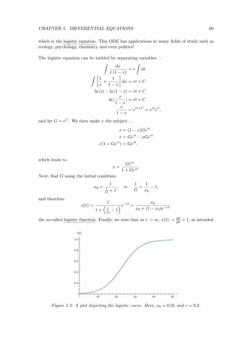
the so-called logistic function. Finally, we note that as t→∞, x(t)→ ��x0��x0
= 1, as intended.
Figure 5.3: A plot depicting the logistic curve. Here, x0 = 0.01 and r = 0.2.
Chapter 6
Vectors
6.1 Introduction
Definition 6.1. A vector is a quantity with both a magnitude (size) and direction.
Many quantities in engineering applications can be described by vectors, e.g. force, velocity,magnetic field.
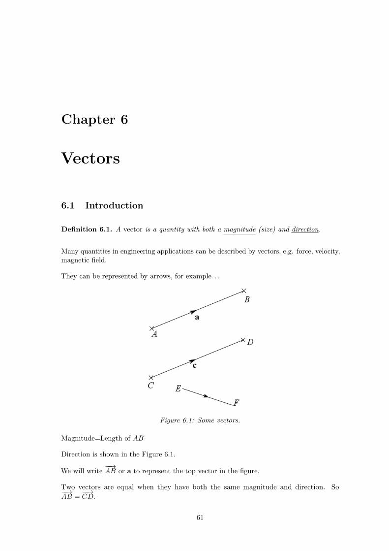
They can be represented by arrows, for example. . .
Figure 6.1: Some vectors.
Magnitude=Length of AB
Direction is shown in the Figure 6.1.
We will write−−→AB or a to represent the top vector in the figure.
Two vectors are equal when they have both the same magnitude and direction. So−−→AB =
−−→CD.
61

CHAPTER 6. VECTORS 62
But−−→AB 6=
−−→EF , since both the magnitude and direction are different.
The sum of two vectors a and b is found by adding the vectors “head to tail”:
Example 6.1 (Forces on an object). Consider the following forces acting on an object:
Forces add to give a net effect or resultant force.
R = F1 + F2
Magnitude: |R| =√
82 + 52 ≈ 9.4N.
Direction: Use tan θ =|F1||F2|
=8
5= 1.6
⇒ θ = 58°.
You can multiply a vector a by a scalar (number) k. Then, as shown in Figure 6.2, if k > 0,ka is a vector in the same direction as a, and the magnitude is k|a|. . . BUT if k < 0, ka isin the opposite direction!
Example 6.2. Two points A and B have position vectors ( i.e. relative to a fixed originO) a and b respectively. What is the position vector of a point on the line joining A andB, equidistant from A and B?
Well, the first thing we need is a sketch of the problem, like in Figure 6.3.
Next, note that−−→AB = b− a.
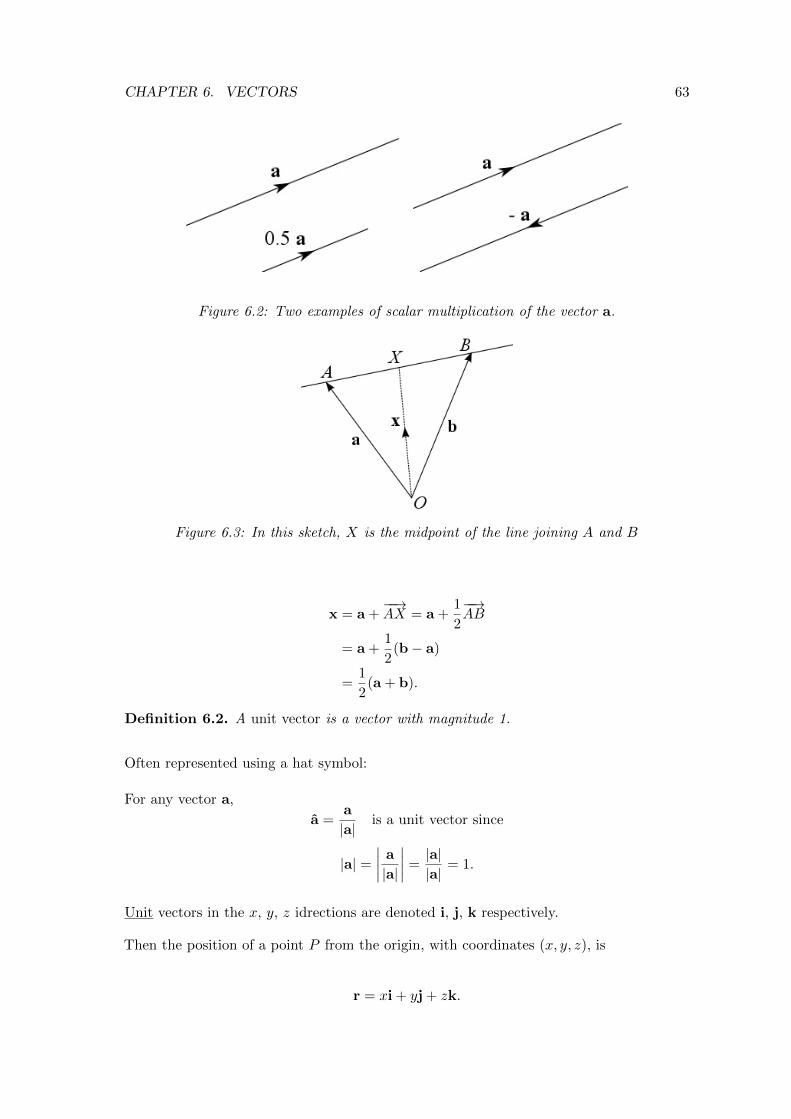
CHAPTER 6. VECTORS 63
Figure 6.2: Two examples of scalar multiplication of the vector a.
Figure 6.3: In this sketch, X is the midpoint of the line joining A and B
x = a +−−→AX = a +
1
2
−−→AB
= a +1
2(b− a)
=1
2(a + b).
Definition 6.2. A unit vector is a vector with magnitude 1.
Often represented using a hat symbol:
For any vector a,
a =a
|a|is a unit vector since
|a| =∣∣∣∣ a
|a|
∣∣∣∣ =|a||a|
= 1.
Unit vectors in the x, y, z idrections are denoted i, j, k respectively.
Then the position of a point P from the origin, with coordinates (x, y, z), is
r = xi + yj + zk.

CHAPTER 6. VECTORS 64
Figure 6.4: ijk
Example 6.3.
a = 6i− 3j + k,
b = 4i + 2j.
Then
a + b = 10i− j− k
b− a = −2i + 5j− k
3a = 18i− 9j + 3k.
For a position vector r = xi + yj + zk, the magnitude is
|r| =√x2 + y2 + z2.
Then for the previous example,
|a| =√
62 + (−3)2 + 12 =√
46,
|b| =√
42 + 22 + 02 = 2√
5.
So far we’ve seen how to add two vectors. Now we have a question. . .
Q: How can we multiply two vectors together?
I’m going to show you that there are in fact two ways to multiply vectors. . .
6.2 The Dot Product
Let us consider the origin of the dot product:
We take two vectors a and b:
We might be interested in the length of the component of a which is in the same directionas b.
Here 0 ≤ θ < π is the angle between a and b.

CHAPTER 6. VECTORS 65
Figure 6.5: The two vectors a and b. We see that the length of the component of a whichis in the same direction as b is |a| cos θ.
Compare with the dot product formula:
a · b = |a||b| cos θ
Looks almost like the length of the component of a, but is rescaled such that we have thesymmetry:
a · b = b · a
So the dot product also gives us a rescaling of the length of the component of b in the samedirection as a. But we expected that in the first place, because of the above symmetryrule!
Figure 6.6: This time, we would like the length of the component of b which is in the samedirection as a. That length is |b| cos θ.
Note that
a · b = |a||b| cos θ ⇒ cos θ =a · b|a||b|
;
which is a useful method for calculating θ if you know a and b.
Two non-zero vectors are perpendicular (orthogonal) if and only if their dot product iszero, i.e.
a.b = 0 ⇒ |a||b| cos θ = 0
⇒ cos θ = 0
⇒ θ =π
2(90°)
Now consider i, j, k. These are unit vectors, and are mutually perpendicular. These twofacts combined show that, e.g.
i · i = 1, i · j = 0, etc.,

CHAPTER 6. VECTORS 66
so if you then let
a = (a1, a2, a3) (= a1i + a2j + a3k)
b = (b1, b2, b3) (= b1i + b2j + b3k),
and multiply out a · b, you obtain
a · b = a1b1 + a2b2 + a3b3.
Note:
a · a =|a||a| cos 0 = |a|2
i.e. |a| =√
a · a.
Let’s try this with r = xi + yj + xk. Then:
|r| =√
r · r =√x2 + y2 + z2,
which is consistent with the earlier formula for the magnitude of r.
Example 6.4. For
a = 6i− 3j + k
b = 4i + 2j,
calculate a · b and find the angle between the two vectors.
a.b = 6× 4 + (−3)× 2 + 1× (0) = 18.
But recalla · b = |a||b| cos θ,
and that|a| =
√46, |b| = 2
√5,
therefore
cos θ =a · b|a||b|
=18
2√
5√
46= 0.593.
∴ θ = cos−1(0.593) = 53.6°.
Example 6.5. Points A,B and C have coordinates (3, 2), (4,−3), (7,−5) respectively.
i Find−−→AB and
−→AC.
ii Find−−→AB·−→AC.
iii Deduce the angle between−−→AB and
−→AC.
i
−−→AB = (4i− 3j)− (3i + 2j) = i− 5j,−→AC = (7i− 5j)− (3i + 2j) = 4i− 7j.
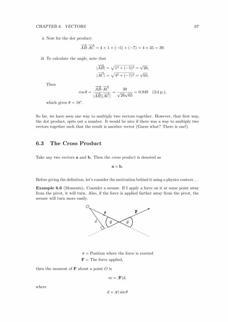
CHAPTER 6. VECTORS 67
ii Now for the dot product:
−−→AB·−→AC = 4× 1 + (−5)× (−7) = 4 + 35 = 39.
iii To calculate the angle, note that
|−−→AB| =
√12 + (−5)2 =
√26,
|−→AC| =
√42 + (−7)2 =
√65.
Then
cos θ =
−−→AB·−→AC
|−−→AB||
−→AC|
=39√
26√
65= 0.949 (3 d.p.),
which gives θ = 18°.
So far, we have seen one way to multiply two vectors together. However, that first way,the dot product, spits out a number. It would be nice if there was a way to multiply twovectors together such that the result is another vector (Guess what? There is one!)
6.3 The Cross Product
Take any two vectors a and b. Then the cross product is denoted as
a× b.
Before giving the definition, let’s consider the motivation behind it using a physics context. . .
Example 6.6 (Moments). Consider a seesaw. If I apply a force on it at some point awayfrom the pivot, it will turn. Also, if the force is applied farther away from the pivot, theseesaw will turn more easily.
r = Position where the force is exerted
F = The force applied,
then the moment of F about a point O is
m = |F|d,
whered = |r| sin θ

CHAPTER 6. VECTORS 68
is the perpendicular distance between O and the line of action of F.
∴ m = |r||F| sin θ.
In fact, the moment vector of F about O, i.e. m, is
m = r× F,
which is perpendicular to both r and F. Moreover, m points in the same direction as theaxis of rotation for the seesaw (here, m points out of the page).
Now, m = |m|, hence the magnitude of m is:
|m| = |r||F| sin θ.
Okay, now I can define the vector product:
Definition 6.3. The cross product of two vectors a and b is
a× b = |a||b| sin θ n,
which is a VECTOR, not a NUMBER. So try not to confuse this with the dot product.
Length of a× b : |a× b| = |a||b| sin θ.Direction of a× b : n, found using the right hand rule.
n is a unit vector perpendicular to a and b.
Figure 6.7: The vectors a, b and a× b. If you put your thumb on a and your index fingeron b, then your middle finger will tell you the direction of a× b.
This definition only works for 3D vectors!
Q: Now, does a× b = b× a?
A: NO!
To see this, let v = a× b and w = b× a. By definition, we will have that |v| = |v|, butwhat about their directions? Well, the right hand rule shows us that v = −w. Hence
b× a 6= a× b!
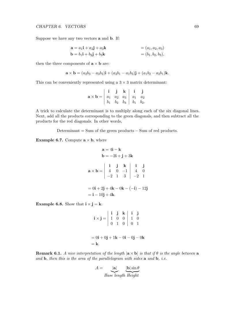
CHAPTER 6. VECTORS 69
Suppose we have any two vectors a and b. If:
a = a1i + a2j + a3k = (a1, a2, a3)
b = b1i + b2j + b3k = (b1, b2, b3),
then the three components of a× b are:
a× b = (a2b3 − a3b2)i + (a3b1 − a1b3)j + (a1b2 − a2b1)k.
This can be conveniently represented using a 3× 3 matrix determinant:
a× b =
∣∣∣∣∣∣i j ka1 a2 a3
b1 b2 b3
∣∣∣∣∣∣i ja1 a2
b1 b2.
A trick to calculate the determinant is to multiply along each of the six diagonal lines.Next, add all the products corresponding to the green diagonals, and then subtract all theproducts for the red diagonals. In other words,
Determinant = Sum of the green products− Sum of red products.
Example 6.7. Compute a× b, where
a = 4i− k
b = −2i + j + 3k
a× b =
∣∣∣∣∣∣i j k4 0 −1−2 1 3
∣∣∣∣∣∣i j4 0−2 1
= 0i + 2j + 4k− 0k− (−i)− 12j
= i− 10j + 4k.
Example 6.8. Show that i× j = k.
i× j =
∣∣∣∣∣∣i j k1 0 00 1 0
∣∣∣∣∣∣i j1 00 1
= 0i + 0j + 1k− 0i− 0j− 0k
= k.
Remark 6.1. A nice interpretation of the length |a×b| is that if θ is the angle between aand b, then this is the area of the parallelogram with sides a and b, i.e.
A = |a|︸︷︷︸Base length
|b| sin θ︸ ︷︷ ︸Height

CHAPTER 6. VECTORS 70
Figure 6.8: A paralellogram, whose sides correspond to vectors a and b. It can be split intotwo triangles.
Proof:A = 2A1,
but
A1 =1
2|a||b| sin θ, [Anyone recognise this trigonometric formula?]
=1
2|a× b|,
henceA = |a× b|.
�
Example 6.9 (Recycled exam question!). Find the area of a triangle with adjacent sidesgiven by
a = i + 2j− k
b = j + k.
Note that
i× j =
∣∣∣∣∣∣i j k1 2 −10 1 1
∣∣∣∣∣∣i j1 20 1
= 2i + 0j + k− (−i)− j− 0k
= 3i− j + k.
We want the area of the shaded region A, but
|a× b| = 2A
⇒ A =1
2|a× b|
=1
2
√32 + (−1)2 + 12
=1
2
√11.
Chapter 7
Numerical Methods
7.1 Introduction
In many cases the integral
I =
∫ b
af(x)dx
can be found by finding a function F (x) such that F ′(x) = f(x), and using
I =
∫ b
af(x)dx = F (b)− F (a)
which is known as the analytical (exact) solution.
But consider ∫ 1
0
√1 + x3 dx, and
∫ 1
0ex
2dx.
Neither of the above integrals can be expressed in terms of functions that we know. Howeverboth of these integrals do exist, since they both represent the area below the curves
√1 + x3
and ex2
between x = 0 and x = 1 (and both curves are well-behaved).
Yet in the above two cases we know what f(x) is. Sometimes, engineers want to calculatean area by computing I, but. . .
• They don’t know the equation for f(x).
• There might be no formula for f(x) at all!
Thankfully, there are some practical methods out there for calculating areas under graphs,e.g. counting squares. But this is time-consuming and boring! Besides, there are othermethods of calculating areas which are much more accurate, even though they are stillonly approximations.
71
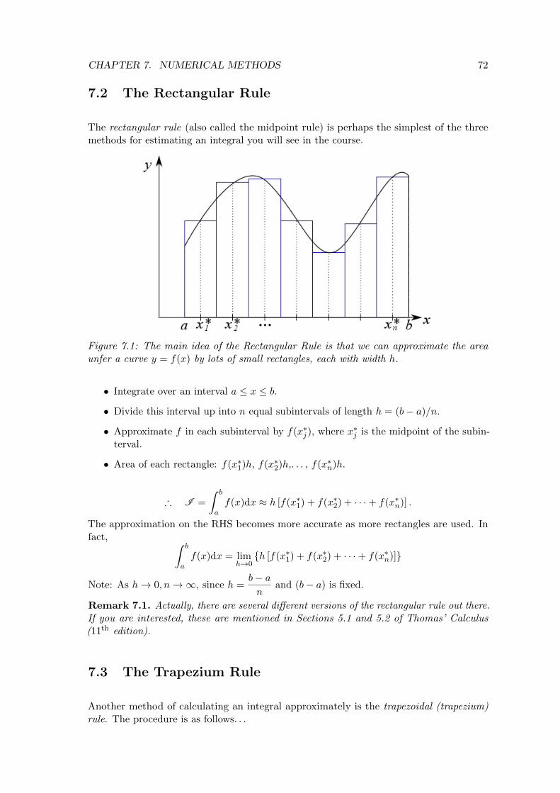
CHAPTER 7. NUMERICAL METHODS 72
7.2 The Rectangular Rule
The rectangular rule (also called the midpoint rule) is perhaps the simplest of the threemethods for estimating an integral you will see in the course.
Figure 7.1: The main idea of the Rectangular Rule is that we can approximate the areaunfer a curve y = f(x) by lots of small rectangles, each with width h.
• Integrate over an interval a ≤ x ≤ b.
• Divide this interval up into n equal subintervals of length h = (b− a)/n.
• Approximate f in each subinterval by f(x∗j ), where x∗j is the midpoint of the subin-terval.
• Area of each rectangle: f(x∗1)h, f(x∗2)h,. . . , f(x∗n)h.
∴ I =
∫ b
af(x)dx ≈ h [f(x∗1) + f(x∗2) + · · ·+ f(x∗n)] .
The approximation on the RHS becomes more accurate as more rectangles are used. Infact, ∫ b
af(x)dx = lim
h→0{h [f(x∗1) + f(x∗2) + · · ·+ f(x∗n)]}
Note: As h→ 0, n→∞, since h =b− an
and (b− a) is fixed.
Remark 7.1. Actually, there are several different versions of the rectangular rule out there.If you are interested, these are mentioned in Sections 5.1 and 5.2 of Thomas’ Calculus(11th edition).
7.3 The Trapezium Rule
Another method of calculating an integral approximately is the trapezoidal (trapezium)rule. The procedure is as follows. . .

CHAPTER 7. NUMERICAL METHODS 73
Again, divide the interval a ≤ x ≤ b into n equal subintervals, i.e.
a = x0 < x1 < x2 < . . . < xn−1 < xn = b,
each with length h = (b− a)/n.
Figure 7.2: The Trapezium Rule visualised. This time, the area under the curve y = f(x)is approximated by a sum of n trapezia, instead of rectangles.
Figure 7.3: This is the first trapezium from Figure 7.2. One way to calculate its area is tosplit it up into a triangle and a rectangle, calculate their areas separately, then add the twoareas together.
Area of first trapezium:A1 = Area of rectangle + Area of triangle
= f(a)h +1
2h(f(x1)− f(a))
=1
2h [f(a) + f(x1)]
Area of next trapezium:A2 =1
2h [f(x1) + f(x2)]
...
Area of penultimate trapezium:An−1 =1
2h [f(xn−2) + f(xn−1)]
Area of last trapezium:An =1
2h [f(xn−1) + f(b)]
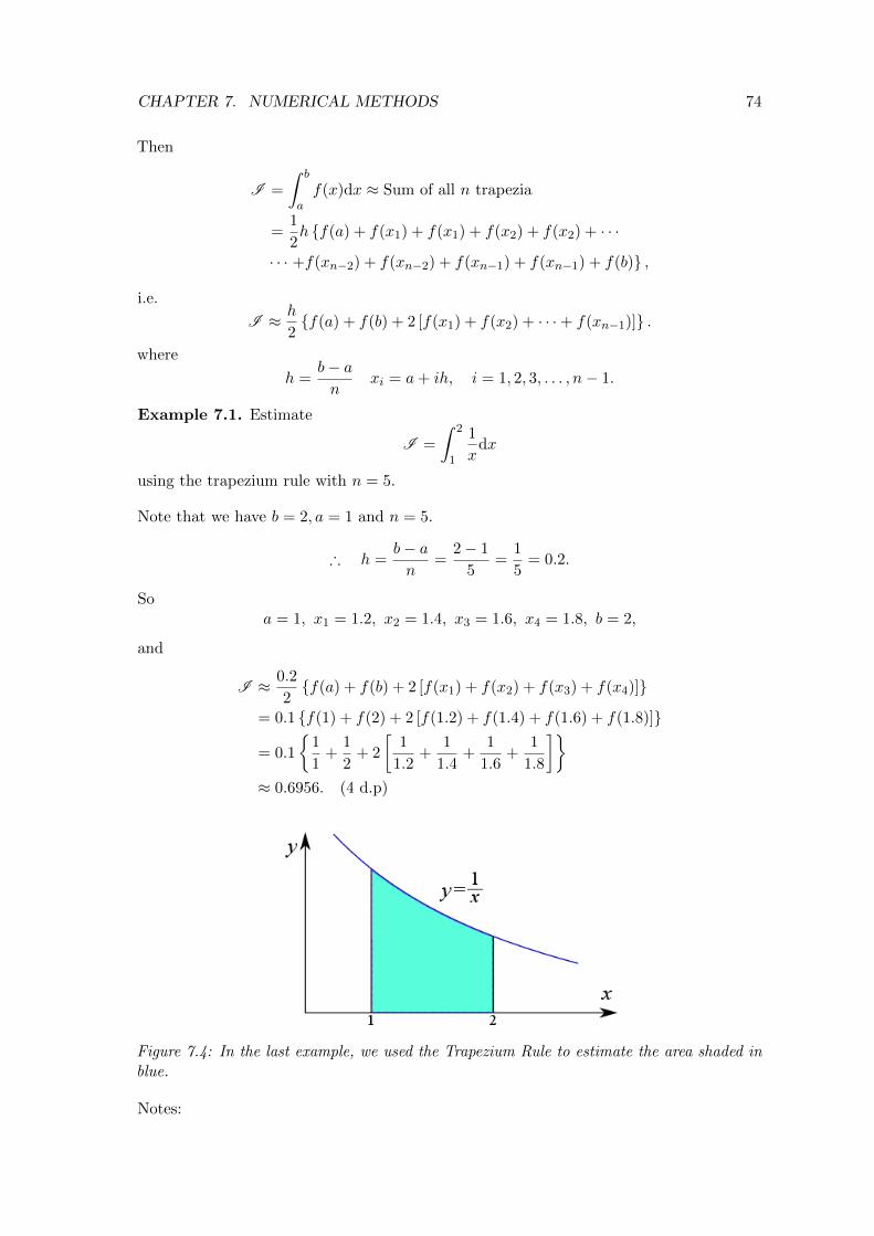
CHAPTER 7. NUMERICAL METHODS 74
Then
I =
∫ b
af(x)dx ≈ Sum of all n trapezia
=1
2h {f(a) + f(x1) + f(x1) + f(x2) + f(x2) + · · ·
· · · +f(xn−2) + f(xn−2) + f(xn−1) + f(xn−1) + f(b)} ,
i.e.
I ≈ h
2{f(a) + f(b) + 2 [f(x1) + f(x2) + · · ·+ f(xn−1)]} .
where
h =b− an
xi = a+ ih, i = 1, 2, 3, . . . , n− 1.
Example 7.1. Estimate
I =
∫ 2
1
1
xdx
using the trapezium rule with n = 5.
Note that we have b = 2, a = 1 and n = 5.
∴ h =b− an
=2− 1
5=
1
5= 0.2.
Soa = 1, x1 = 1.2, x2 = 1.4, x3 = 1.6, x4 = 1.8, b = 2,
and
I ≈ 0.2
2{f(a) + f(b) + 2 [f(x1) + f(x2) + f(x3) + f(x4)]}
= 0.1 {f(1) + f(2) + 2 [f(1.2) + f(1.4) + f(1.6) + f(1.8)]}
= 0.1
{1
1+
1
2+ 2
[1
1.2+
1
1.4+
1
1.6+
1
1.8
]}≈ 0.6956. (4 d.p)
Figure 7.4: In the last example, we used the Trapezium Rule to estimate the area shaded inblue.
Notes:
CHAPTER 7. NUMERICAL METHODS 75
• In the previous example, the analytical value is given by∫ 2
1
1
xdx = [lnx]21 = ln 2− ln 1 = ln 2 = 0.6931 (4.d.p).
• If we used n = 10, we would have
I ≈ 0.6938,
which is even more accurate than using n = 5.
Error in using the Trapezuim Rule
Let I be the trapezium approximation to I , then we define the error εT as
εT = I −I .
Then it turns out that if ∣∣f ′′(x)∣∣ ≤M for all x with a ≤ x ≤ b,
then
|εT | ≤M(b− a)3
12n2.
Example 7.2. What is the smallest n such that
I =
∫ 2
0ex
2dx
has a maximum error of 1?
We must choose n large enough such that |εT | ≤ 1. Note that
f(x) = ex2 ⇒ f ′′(x) =
[2 + 4x2
]ex
2
We are interested in 0 ≤ x ≤ 2; on this interval the maximum value of f ′′(x) occurs atx = 2, thus M = f ′′(2) ≈ 983 (rounded up). So
|εT | ≤M(b− a)3
12n2≤ 983
23
12n2≈ 655
n2
i.e we need655
n2≤ 1 ⇒ n2 ≥ 655.
The smallest such n that satisfies this is n = 26.
7.4 Simpson’s Rule
Simpson’s Rule is yet another method of numerical integration. It is credited to ThomasSimpson (1710-1761), an English mathematician, though there is evidence that similarmethods were used 100 years prior to him.
So far, we looked at two methods for numerical integration:

CHAPTER 7. NUMERICAL METHODS 76
• Piecewise constant approximation =⇒ Rectangular Rule
• Piecewise linear approximation =⇒ Trapezium Rule
• Piecewise quadratic approximation =⇒ Simpson’s Rule
For Simpson’s rule we divide a ≤ x ≤ b into an even number of subintervals n of lengthh = (b− a)/n with endpoints
a = x0 < x1 < x2 < . . . < xn−1 < xn = b,
Main idea: Suppose a typical parabola Pi (i.e. ax2+bx+c) passes through three consecutivepoints (xi−1, yi−1), (xi, yi), (xi+1, yi+1).
Figure 7.5: Simpson’s Rule visualised. For this method, the curve y = f(x) is approximatedusing n parabolae; then the area underneath the parabolae is taken as the approximate valueof the integral.
We will not go through the derivation, but I can tell you that Simpson’s formula turns outto be. . .
h
3(S0 + 4S1 + 2S2) ,
where
S0 = f(a) + f(b), (7.1)
S1 = f(x1) + f(x3) + f(x5) + . . .+ f(xn−1), (7.2)
S2 = f(x2) + f(x4) + f(x6) + . . .+ f(xn−2). (7.3)
(7.4)
Observe that for all the indices that appear in S1, are odd, while those for S2 are even(remember that as n must be even, we have that (n− 1) is odd whilst (n− 2) is even).Meanwhile it can be shown for Simpson’s rule that if
|f (4)(x)| ≤M for all x with a ≤ x ≤ b,

CHAPTER 7. NUMERICAL METHODS 77
then
|εS | ≤M(b− a)5
180n4.
Example 7.3. Evaluate
I =
∫ 2
1
1
xdx
using Simpson’s rule with n = 10, a = 1, b = 2.
Note that
h =2− 1
10=
1
10= 0.1,
and keep track of all the values of xi and f(xi) as follows. . .
i xi f(xi) = 1/xi
0 1.0 11 1.1 10/112 1.2 5/63 1.3 10/134 1.4 5/75 1.5 2/36 1.6 5/87 1.7 10/178 1.8 5/99 1.9 10/1910 2.0 1/2
Sums 1.5000000 3.459539 2.728175
i.e.
S0 = 1.500000
S1 = 3.459539
S2 = 2.728175
and therefore
I =h
3(S0 + 4S1 + 2S2) = 0.693150.
Compare with the exact value
I =
∫ 2
1
dx
x= ln 2 = 0.69314718,
hence this is correct to FIVE d.p. (Trapezium Rule was correct to 1 d.p.)
7.5 Newton’s Method for Root-Finding
In engineering, it is often required to find x such that
f(x) = 0. (7.5)
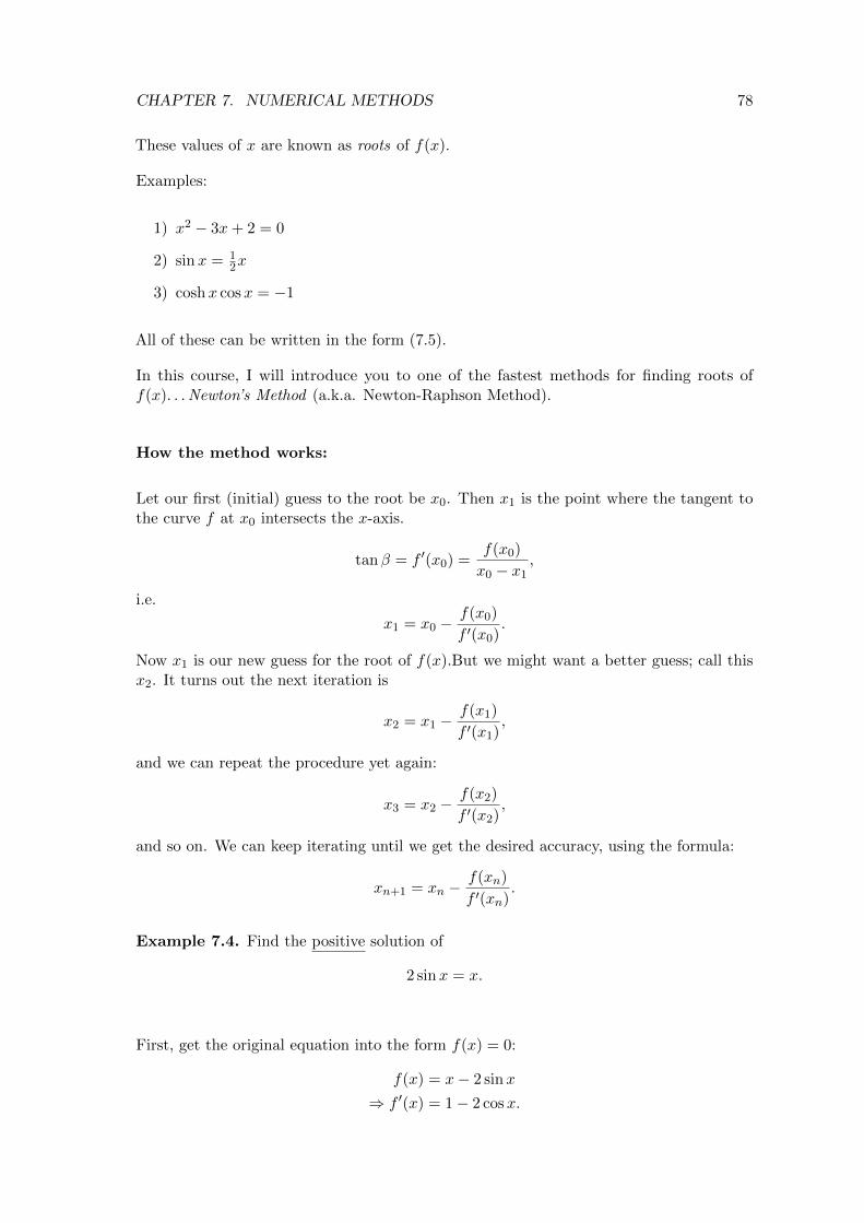
CHAPTER 7. NUMERICAL METHODS 78
These values of x are known as roots of f(x).
Examples:
1) x2 − 3x+ 2 = 0
2) sinx = 12x
3) coshx cosx = −1
All of these can be written in the form (7.5).
In this course, I will introduce you to one of the fastest methods for finding roots off(x). . . Newton’s Method (a.k.a. Newton-Raphson Method).
How the method works:
Let our first (initial) guess to the root be x0. Then x1 is the point where the tangent tothe curve f at x0 intersects the x-axis.
tanβ = f ′(x0) =f(x0)
x0 − x1,
i.e.
x1 = x0 −f(x0)
f ′(x0).
Now x1 is our new guess for the root of f(x).But we might want a better guess; call thisx2. It turns out the next iteration is
x2 = x1 −f(x1)
f ′(x1),
and we can repeat the procedure yet again:
x3 = x2 −f(x2)
f ′(x2),
and so on. We can keep iterating until we get the desired accuracy, using the formula:
xn+1 = xn −f(xn)
f ′(xn).
Example 7.4. Find the positive solution of
2 sinx = x.
First, get the original equation into the form f(x) = 0:
f(x) = x− 2 sinx
⇒ f ′(x) = 1− 2 cosx.

CHAPTER 7. NUMERICAL METHODS 79
Figure 7.6: In the last example, we used the Trapezium Rule to estimate the area shaded inblue.
Figure 7.7: A plot of y = 2 sinx and y = x. The root we are after is the positive x-value atthe point where the two functions intersect.
Then, by Newton’s Method,
xn+1 = xn −xn − 2 sinxn1− 2 cosxn
=2(sinxn − xn cosxn)
1− 2 cosxn=Nn
Dn.
We need an initial guess, e.g. x0 = 2.
n xn Nn Dn xn+1 = Nn/Dn
0 2.00 3.483 1.832 1.9011 1.901 3.125 1.648 1.8962 1.896 3.107 1.639 1.896
The actual solution to 4 d.p is 1.8955.

CHAPTER 7. NUMERICAL METHODS 80
Advantages of Newton’s method:
• Converges very fast!
• You only need to give one initial guess (some methods require TWO).
Disadvantages:
• You need to calculate the derivative of f(x).
• Sometimes the method doesn’t converge to a root at all!
• The method is useless if your first guess is a stationary point of f(x) (because youget a division by zero).
Chapter 8
Probability and Statistics
8.1 Basic Probability
For an event E, the probability of the E occurring, denoted P(E), is a number such that
0 ≤ P(E) ≤ 1.
where
P(E) = 0 =⇒ E is impossible,
P(E) = 1 =⇒ E is certain.
Example 8.1 (Rolling a die). The set of all possible outcomes is the sample space, denotedS, i.e.
S = {1, 2, 3, 4, 5, 6} .
Let A be the event of getting an even number in one roll. Then we have
A = {2, 4, 6}
and therefore
P(A) =3
6=
1
2.
Example 8.2. We randomly select 2 lightbulbs from a set of 5 bulbs (numbered 1 to 5).The sample space consists of 10 possible outcomes:
S = {{1, 2}, {1, 3}, {1, 4}, {1, 5}, {2, 3},{2, 4}, {2, 5}, {3, 4}, {3, 5}, {4, 5}} .
Note that |S| = 10 is the number of elements in S, also known as the cardinality of the setS. We may be interested in the following events:
A: No faulty bulbs
B: One faulty bulb
C: Two faulty bulbs
81

CHAPTER 8. PROBABILITY AND STATISTICS 82
Now assume that bulbs 1, 2 and 3 are all faulty. We see that event A occurs only if wedraw bulbs 4 and 5 (i.e. outcome {4, 5}).
∴ P (A) =1
10.
Event B occurs if we draw {1, 4} , {1, 5} , {2, 4} , {2, 5} , {3, 4} or {3, 5}. Hence
P (B) =6
10.
Meanwhile, Event C occurs if we draw {1, 2} , {1, 3} , {2, 3}, and therefore
P (C) =3
10.
Definition 8.1. The set of all elements (outcomes) not in E in the sample space S iscalled the compliment of E, usually denoted Ec or E.
Example 8.3. E = randomly rolled die gives an even number, i.e.
E = {2, 4, 6} ,
then Ec = randomly rolled die gives an odd number, i.e.
Ec = {1, 3, 5} .
Let A and B be two events in an experiment.
Definition 8.2. The event consisting of all the elements of the sample space that belongto either A or B is called the union of A and B and is denoted as A ∪B.
Figure 8.1: A Venn diagram. The union A ∩B is shaded in green.
Definition 8.3. The event consisting of all the elements of the sample space that belongto both A and B is called the intersection of A and B and is denoted as A ∩B.
Example 8.4. Suppose that we are rolling a die, then consider the following events:
A: The die gives a number not smaller than 4.
B: The die gives a number that is a multiple of 3.
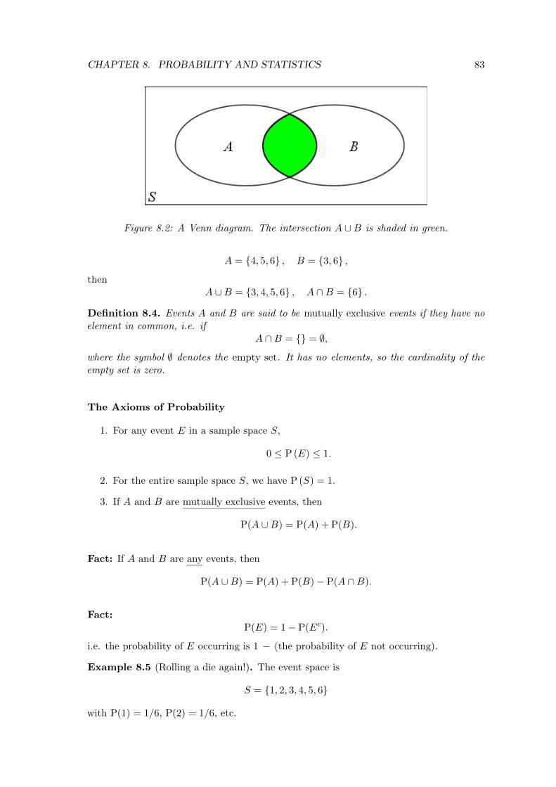
CHAPTER 8. PROBABILITY AND STATISTICS 83
Figure 8.2: A Venn diagram. The intersection A ∪B is shaded in green.
A = {4, 5, 6} , B = {3, 6} ,
thenA ∪B = {3, 4, 5, 6} , A ∩B = {6} .
Definition 8.4. Events A and B are said to be mutually exclusive events if they have noelement in common, i.e. if
A ∩B = {} = ∅,
where the symbol ∅ denotes the empty set. It has no elements, so the cardinality of theempty set is zero.
The Axioms of Probability
1. For any event E in a sample space S,
0 ≤ P (E) ≤ 1.
2. For the entire sample space S, we have P (S) = 1.
3. If A and B are mutually exclusive events, then
P(A ∪B) = P(A) + P(B).
Fact: If A and B are any events, then
P(A ∪B) = P(A) + P(B)− P(A ∩B).
Fact:P(E) = 1− P(Ec).
i.e. the probability of E occurring is 1 − (the probability of E not occurring).
Example 8.5 (Rolling a die again!). The event space is
S = {1, 2, 3, 4, 5, 6}
with P(1) = 1/6, P(2) = 1/6, etc.

CHAPTER 8. PROBABILITY AND STATISTICS 84
A: The event that an even number is given.
P(A) = P(2) + P(4) + P(6) =1
2.
B: The event that a number greater than 4 turns up.
P(B) = P(5) + P(6) =1
3.
Example 8.6. Five coins are tossed simultaneously. What is the probability of obtainingat least one head?
Note: There are in total 25 = 32 possible outcomes, only one of which has no heads.Therefore
P(At least one head) = 1− P(No heads)
= 1− 1
32=
31
32.
Example 8.7. The probability that a person watches TV is P(T ) = 0.6; the probabilitythat the same person listens to the radio P(R) = 0.3. The probability that they do both is0.15. What is the probability that they do neither?
Using the addition law,
P(T ∪R) = P(T ) + P(R)− P(T ∩R)
= 0.6 + 0.3− 0.15 = 0.75.
∴ P(They do neither) = 1− P(T ∪R) = 0.25.
Conditional probability
Often it is required to find the probability of an event B given that an event A has alreadyoccurred. This is known as the conditional probability of B given A, and is denoted P(B|A).
The intuition behind this is that A gives a “reduced sample space”, and therefore
P(B|A) =P(A ∩B)
P(A).
Example 8.8 (Conditional Probability). The probability P(A) that it rains in Manchester
on July 15th is 0.6, while the probability P(A ∩B) that it rains there on both the 15th
and 16th is 0.35. Given that it rains on the 15th, what is the probability that it rains onthe next day?
Note: B is the event that it rains in Manchester on July 16th. We need to find P(B|A),and using the formula for conditional probability :
P(B|A) =PA ∩B
P(A)=
0.35
0.6=
7
12= 0.583. (3 d.p)

CHAPTER 8. PROBABILITY AND STATISTICS 85
Example 8.9. A fridge contains 10 cans of lager, three of which are “4X” (to be avoided).Robb selects 2 cans at random. Find the probability that none of the selected cans are“4X”.
Let A = First can selected is not 4X,
B = Second can selected is not 4X.
We will look at two different cases. . .
1 The case with replacement, i.e. Robb puts the first can back in the fridge beforechoosing the second. Then
P(A) = P(B) =7
10,
and
P(A ∩B) =7
10× 7
10= 0.49.
2 Sampling without replacement, i.e. the first can is NOT put back in the fridge.Then. . .
P(A) =7
10, and P(B|A) =
7× 1
10× 1=
6
9=
2
3.
∴ P(A ∩B) = P(A) P(B|A) =7
10× 2
3=
14
30≈ 0.47.
8.2 Random Variables
Sometimes engineers must work with a variable X whose (real) value is subject to variationsdue to chance (randomness). We call X a random variable.
So X can take on a set of possible different values, each with a corresponding probability.We can say that for each possible value a, for
X = a the probability of this value is P(X = a).
We can then say that the probability that X assumes any value within the range:
1. b < X < c is P(b < X < c)
2. X ≤ c is P(X ≤ c)
3. X > c is P(X > c).
Actually,P(X ≤ c) + P(X > c) = P(All possible values of X) = 1,
or equivalently,P(X > c) = 1− P(X ≤ c).
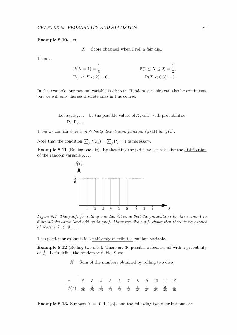
CHAPTER 8. PROBABILITY AND STATISTICS 86
Example 8.10. Let
X = Score obtained when I roll a fair die..
Then. . .
P(X = 1) =1
6, P(1 ≤ X ≤ 2) =
1
3,
P(1 < X < 2) = 0, P(X < 0.5) = 0.
In this example, our random variable is discrete. Random variables can also be continuous,but we will only discuss discrete ones in this course.
Let x1, x2, . . . be the possible values ofX, each with probabilities
P1,P2, . . .
Then we can consider a probability distribution function (p.d.f) for f(x).
Note that the condition∑
j f(xj) =∑
j Pj = 1 is necessary.
Example 8.11 (Rolling one die). By sketching the p.d.f, we can visualise the distributionof the random variable X. . .
Figure 8.3: The p.d.f. for rolling one die. Observe that the probabilities for the scores 1 to6 are all the same (and add up to one). Moreover, the p.d.f. shows that there is no chanceof scoring 7, 8, 9, . . .
This particular example is a uniformly distributed random variable.
Example 8.12 (Rolling two dice). There are 36 possible outcomes, all with a probabilityof 1
36 . Let’s define the random variable X as:
X = Sum of the numbers obtained by rolling two dice.
x 2 3 4 5 6 7 8 9 10 11 12
f(x) 136
236
336
436
536
636
536
436
336
236
136
Example 8.13. Suppose X = {0, 1, 2, 3}, and the following two distributions are:

CHAPTER 8. PROBABILITY AND STATISTICS 87
Figure 8.4: The p.d.f. for rolling two dice. Unsurprisingly, there is zero chance of gaininga sum of thirteen!
i f(x) = 18(1 + x)
ii f(x) = 110(1 + x).
Only one of these is a valid p.d.f. Which one, and why?
Answer: (ii) is valid, but (i) is not.Why: Need
∑j f(xj) = 1. Only (ii) satisfies it.
Definition The mean, expectation or expected value µ of a discrete p.d.f:
[(E(X) =] µ =∑j
xjf(xj) = x1f(x1) + x2f(x2) + · · · .
Example 8.14 (Expected value for rolling a fair die). Recall that
f(xj) =1
6when j = 1, 2, . . . , 6
⇒ µ = 1× 1
6+ 2× 2
6+ . . .+ 6× 6
6= 3.5.
Granted, we can’t gain a score of 3.5 if we roll the die only once. But that is not whatµ means. Actually, µ represents the average “score” you would get if you rolled the diemany times.
Example 8.15. A stranger shows you a game where you draw a ball out of a bag. Thereare 6 white balls and 4 blue balls in the bag.
• If the ball is white, you win 40p.
• If the ball is blue, you lose 80p.
Afterwards, the ball is replaced. What are your expected winnings? And is it worth playingthat game?
Let X = winnings obtained after drawing the ball out.
When X = 40 (x1) P(x1) =6
10,
X = −80 (x2) P(x2) =4
10.
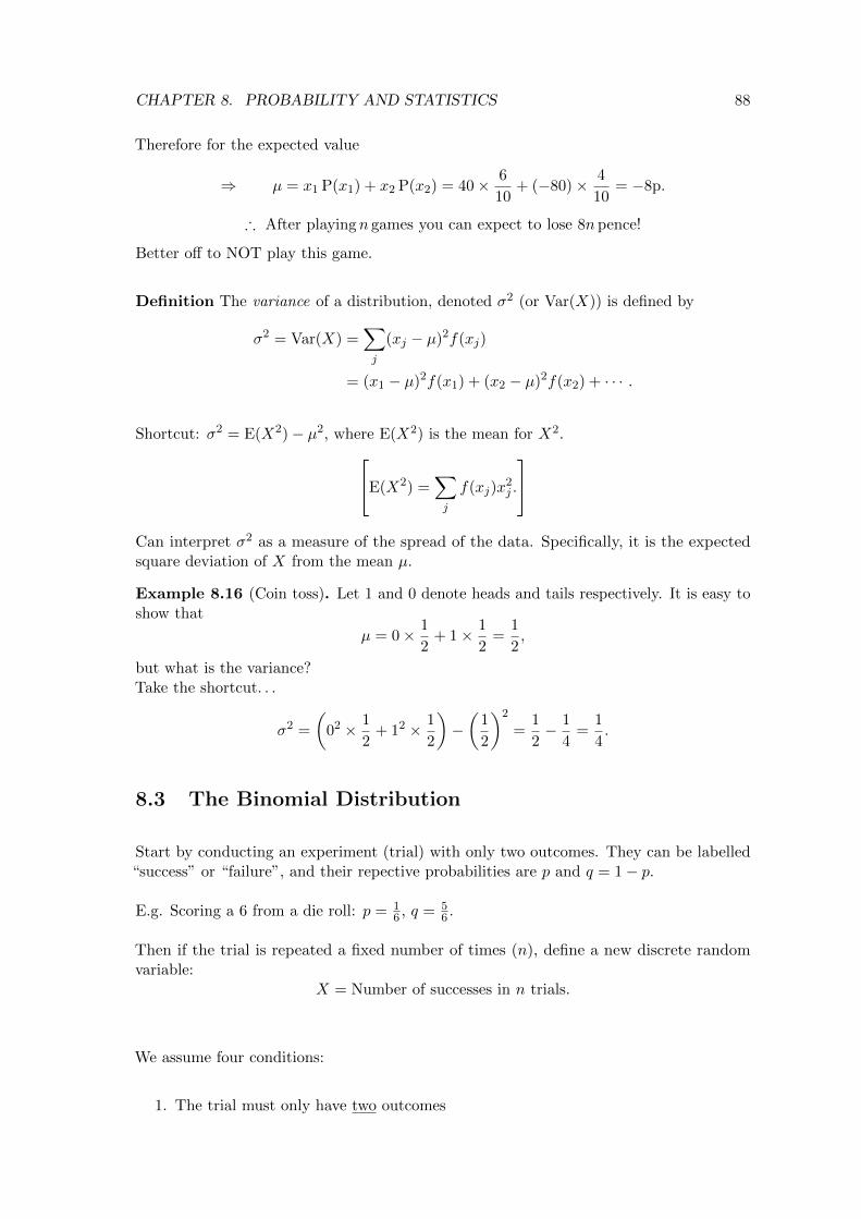
CHAPTER 8. PROBABILITY AND STATISTICS 88
Therefore for the expected value
⇒ µ = x1 P(x1) + x2 P(x2) = 40× 6
10+ (−80)× 4
10= −8p.
∴ After playingn games you can expect to lose 8n pence!
Better off to NOT play this game.
Definition The variance of a distribution, denoted σ2 (or Var(X)) is defined by
σ2 = Var(X) =∑j
(xj − µ)2f(xj)
= (x1 − µ)2f(x1) + (x2 − µ)2f(x2) + · · · .
Shortcut: σ2 = E(X2)− µ2, where E(X2) is the mean for X2.E(X2) =∑j
f(xj)x2j .
Can interpret σ2 as a measure of the spread of the data. Specifically, it is the expectedsquare deviation of X from the mean µ.
Example 8.16 (Coin toss). Let 1 and 0 denote heads and tails respectively. It is easy toshow that
µ = 0× 1
2+ 1× 1
2=
1
2,
but what is the variance?Take the shortcut. . .
σ2 =
(02 × 1
2+ 12 × 1
2
)−(
1
2
)2
=1
2− 1
4=
1
4.
8.3 The Binomial Distribution
Start by conducting an experiment (trial) with only two outcomes. They can be labelled“success” or “failure”, and their repective probabilities are p and q = 1− p.
E.g. Scoring a 6 from a die roll: p = 16 , q = 5
6 .
Then if the trial is repeated a fixed number of times (n), define a new discrete randomvariable:
X = Number of successes in n trials.
We assume four conditions:
1. The trial must only have two outcomes

CHAPTER 8. PROBABILITY AND STATISTICS 89
2. Fixed number of trials
3. The probability of success must be the same for all trials
4. The trials are independent.
Example 8.17. Find the probability of 0,1,2,3,4 successes in an experiment consisting ofup to 4 repeated trials with probability of success p (∴ q = 1− p).
Number of Trials 1 2 3 4
Number of Successes
0 q q2 q3 q4
1 p 2pq 3pq2 4pq3
2 0 p2 3p2q 6p2q2
3 0 0 p3 4p3q
4 0 0 0 p4
Generally, we can consider the p.d.f. f(x) = P(X = x). Then the probability of x successesin n trials is
P(X = x) =
(n
x
)pxqn−x,
where(nx
)is the binomial coefficient, and the p.d.f. corresponds to the Binomial Distribu-
tion.
Recall that (n
x
)=
n!
x!(n− x)!
These binomial coefficients represent the number of ways of choosing x objects from a setof n objects.
Example 8.18. We roll a die 56 times. What is the probability of getting at least threesixes?
Define a random variable X as
X = Number of sixes thrown in 56 trials.
Then we say that
X ∼ B
(n = 56, p =
1
6
)Then we want
P(≥ 3) = 1− P(X = 0, 1 or 2)
1−
[(5
6
)56
+
(56
1
)(5
6
)55(1
6
)+
(56
2
)(5
6
)54(1
6
)2]
Note: It is perfectly fine to leave your answer in this form!
CHAPTER 8. PROBABILITY AND STATISTICS 90
Example 8.19. A factory produces plenty of board pens. However, 10% of the pens aredefective. If I open a random box containing twenty board pens, what is the probabilitythat:
i Exactly 3 pens are defective?
ii More than 3 pens are defective?
(Answer to 3 decimal places)
First, if X = number of faulty pens in a box of 20,
X ∼ B(20, 0.1)
i We want
P(X = 3) =
(20
3
)(0.1)3(0.9)17 ≈ 0.190.
ii This is P(X ≥ 3), i.e.
P(X ≥ 3) = 1− P(X ≤ 2)
= 1−[0.920 +
(20
1
)(0.1)(0.9)19 +
(20
2
)(0.1)2(0.9)18
]≈ 0.323.
Mean and variance of B(n, p)
Since
f(x) =
(n
x
)pxq1−x,
it turns out that
Mean: µ =
n∑x=0
xf(x) =
n∑x=0
(n
x
)pxqn−xx = np
Variance: σ2 = npq = np(1− p).
So for the board pen example, µ = 2, σ2 = 1.8.
8.4 The Poisson Distribution
Consider the following scenarios:
i Number of phone calls arriving at a call centre per hour.
ii Number of cars crossing a bridge per hour.

CHAPTER 8. PROBABILITY AND STATISTICS 91
iii Number of faults in a length of cable.
These problems require a distribution that involves an average rate µ. Actually, there isone - it is the Poisson distribution, and its p.d.f. is:
P(X = x) =e−µµx
x!,
where X = 0, 1, 2, . . . , to ∞.
Example 8.20. On average, 240 cars per hour pass a check point, and a queue forms ifmore than three cars pass through in a given minute.
What is the probability of a queue forming in a randomly selected minute?
Average number of cars per minute =240
60= 4 = µ.
LetX = Number of cars passing at a randomly selected minute.
Then X ∼ Po(4), and we require
P(X ≥ 3) = 1− P(0 ≤ X ≤ 3)
1− [P(X = 0) + P(X = 1) + P(X = 2) + P(X = 3)]
= 1− 0.4331 = 0.5669.
One important use of the Poisson distribution is to APPROXIMATE the Binomial distri-bution, because Poisson is easier to compute.
Recall that for binomial,
f(x) =
(n
x
)pxqn−x.
Then if you let p −→ 0 and n −→∞ with µ = np fixed and finite,
f(x) −→ Po(µ).
Moreover, the Poisson distribution has mean µ and variance µ.
Example 8.21. A factory produces screws. The probability that a randomly selectedscrew is defective is given by p = 0.01.
In a random sample of 100 screws, what is the probability that there will be morethan two defective screws?
Let A = More than two defective screws
⇒ AC = At most 1 defective.
P(AC) =
(100
0
)(0.01)0(0.99)100 +
(100
1
)(0.01)1(0.99)99
+
(100
2
)(0.01)2(0.99)98.
CHAPTER 8. PROBABILITY AND STATISTICS 92
After spending ages on your calculator, you finally get
⇒ P(A) = 1− P(AC) ≈ 0.0794. (3 s.f.)
Alternative: Poisson approximation. As n is large and p small, we have
µ = np = 1, ∴ 1 out of 100 defective on average.
⇒ P(AC) ≈ e−1
(10
0!+
11
1!+
12
2!
)= ×5
2e−1 ≈ 0.9197,
andP(A) = 1− P(AC) ≈ 0.0803. Close to the binomial result!


![CE 6501 ITS [Compatibility Mode]](https://static.documents.pub/doc/80x56/577cd3161a28ab9e7896a680/ce-6501-its-compatibility-mode.jpg)


