arX

iv:c

s/06

0509

0v3

[cs

.MS]

17

Oct

200

8

Mathematica: A System of ComputerPrograms

Santanu K. Maiti

E-mail: santanu.maiti@saha.ac.in

Theoretical Condensed Matter Physics DivisionSaha Institute of Nuclear Physics

1/AF, Bidhannagar, Kolkata-700 064, India

1

Contents

Preface 3

1 Introduction 4

2 Start with Mathematica 4

2.1 Use of a Mathematica Notebook . . . . . . . . . . . . . . . . . . . . . . 5

2.2 Way of Writing a Program in Mathematica . . . . . . . . . . . . . . . . 5

2.2.1 Characterization of Local and Global Variables . . . . . . . . . 7

3 Way to Link External Programs in Mathematica by Proper Math-

Link Commands 8

3.1 Mathlink for XL Fortran-90 Source Files . . . . . . . . . . . . . . . . . 9

3.1.1 Compilation and Optimization of XL Fortran-90 Source Files . . 10

3.1.2 Link of XL Fortran-90 Program with Mathematica . . . . . . . 11

3.1.3 Link of other XL Fortran Programs with Mathematica . . . . . 13

4 Way to Create a Mathematica Batch-file and Run it in Background 13

5 Parallel Evaluation of Mathematica Programs 15

5.1 How to Open Mathematica Slaves in Local Computer ? . . . . . . . . . 16

5.2 How to Open Mathematica Slaves in Remote Computers Available in

Network ? . . . . . . . . . . . . . . . . . . . . . . . . . . . . . . . . . . 17

5.3 Parallelizing of Mathematica Programs by using Remote Computers

Available in Network . . . . . . . . . . . . . . . . . . . . . . . . . . . . 18

Concluding Remarks 21

Acknowledgment 22

References 22

2

Preface

Mathematica is a powerful application package for doing mathematics and is used al-

most in all branches of science. It has widespread applications ranging from quantum

computation, statistical analysis, number theory, zoology, astronomy, and many more.

Mathematica gives a rich set of programming extensions to its end-user language, and it

permits us to write programs in procedural, functional, or logic (rule-based) style, or a

mixture of all three. For tasks requiring interfaces to the external environment, math-

ematica provides mathlink, which allows us to communicate mathematica programs

with external programs written in C, C++, F77, F90, F95, Java, or other languages.

It has also extensive capabilities for editing graphics, equations, text, etc.

In Section 2, we start from the basic level of mathematica and illustrate how to

use a mathematica notebook and write a program in the notebook. Following with

this, here we also describe very briefly about the importance of the local and global

variables those are used in writing programs in mathematica.

Next, in Section 3, we investigate elaborately the way of linking of external programs

with mathematica, so-called the mathlink operation. Using this technique we can run

very tedious jobs quite efficiently, and the operations become extremely fast.

Sometimes it is quite desirable to run jobs in background of a computer which can

take considerable amount of time to finish, and this allows us to do work on other tasks,

while keeping the jobs running. The way of running jobs, written in a mathematica

notebook, in background is quite different from the conventional methods i.e., the

techniques for the programs written in other languages like C, C++, F77, F90, F95,

etc. To illustrate it, in Section 4, we study how to create a mathematica batch-file

from a mathematica notebook and run it in the background.

Finally, in Section 5, we explore the most significant issue of this article. Here we

describe the basic ideas for parallelizing a mathematica program by sharing its inde-

pendent parts into all other remote computers available in the network. Doing the par-

allelization, we can perform large computational operations within a very short period

of time, and therefore, the efficiency of the numerical works can be achieved. Parallel

computation supports any version of mathematica and it also works significantly well

even if different versions of mathematica are installed in different computers.

All the operations studied in this article run under any supported operating sys-

tem like Unix, Windows, Macintosh, etc. For the sake of our illustrations, here we

concentrate all the discussions only for the Unix based operating system.

3

1 Introduction

Mathematica, a system of computer programs, is a high-level computing environment

including computer algebra, graphics and programming. Mathematica is specially

suitable for mathematics, since it incorporates symbolic manipulation and automates

many mathematical operations. The key intellectual aspect of Mathematica is the

invention of a new kind of symbolic computation language that can manipulate the very

wide range of objects needed to achieve the generality required for technical computing

by using a very small number of basic primitives. Just a single line sometimes makes

a meaningful program in mathematica–the syntax, documents and methodology used

for input and output remaining as they are for immediate calculations. It supports

every type of operation–be they data, functions, graphics, programs, or even complete

documents–to be represented in a single, uniform way as a symbolic expression. This

unification has many practical benefits to broadening the scope of applicability of

each function. The raw algorithmic power of mathematica is magnified and its utility

extended. Mathematica is now emerging as an important tool in many branches of

computing, and today it stands as the world’s best system for general computation.

Mathematica has widespread applications in different fields and is often used for

research, loading and analyzing data, giving technical presentations and seminars etc.

Mathematica is extraordinary well-rounded. It is suitable for both numeric and sym-

bolic work, and it has remarkable word-processing capabilities as well. Mathematicians

can search for a working model, do intensive calculation, and write a dissertation on

the project (including complex graphics) – all from within mathematica. It is math-

ematica’s complete consistency in design at every stage that gives it this multilevel

capability and helps advanced usage evolve naturally.

2 Start with Mathematica

We generally use mathematica through documents called notebooks. To start a math-

ematica notebook in Unix we write ‘mathematica &’ from a command line and then

press the ‘Enter’ key from the key-board. A typical notebook consists of cells that may

contain graphics, texts, programs or calculations. Now to exit from a mathematica

notebook we first go to the command ‘File’ and then press ‘Quit’ from the menu bar of

the notebook. Without using a notebook one can also use mathematica by typing the

command ‘math’ from a command line and all the jobs can also be done as well. To

4

exit from mathematica for this particular case, we should write either ‘Exit’ or ‘Quit’

and then press the ‘Enter’ key. Thus one can run mathematica by using any one of

the above two ways, but the most general way to do the interactive calculations in

mathematica is the use of mathematica through notebook documents.

2.1 Use of a Mathematica Notebook

In a notebook, a job is performed in a particular cell and for different jobs we use

different cells. One can also use a single cell for all the operations, but it is quite

easy if different operations are performed in separate cells. A cell is automatically

created when we begin to write anything in the notebook. After writing proper opera-

tion/operations, it is needed to run the jobs. For this purpose, we press the key ‘Shift’

and holding this key, we then press ‘Enter’ from the key-board. The results for the

inputs are evaluated and they are available immediately underneath in a separate cell,

so-called the output cell.

In mathematica we can do all kind of mathematical operations like numerical com-

putation, algebric computation, matrix manipulation, different types of graphics etc.,

and all these things are clearly described by several examples in key mathematica book

of Wolfram Research [1]. So in this article we shall not give any such example further.

Now to do large numerical computations, it is needed to write a complete program. For

this purpose, here we describe something about the way of writing a complete program

in a mathematica notebook.

2.2 Way of Writing a Program in Mathematica

In mathematica, we can write a program efficiently compared to any other existing

languages. As illustrative example, here we mention a very simple program which is:

the generation of a list of two random numbers and the creation of a 2D plot from these

numbers.

The program is:

sample[times−]:=Block[{local variables},

numbers=Table[{Random[], Random[]}, {i, 1, times}];figure=ListPlot[numbers, PlotJoined→True, AxesLabel→{xlabel, ylabel}]]

This is the complete program for the generation of a list of two random numbers and

the creation of a 2D plot from these numbers. This program is written in a single cell.

5

After the end of this program we run it by using the command ‘SHIFT’ + ‘ENTER’,

and then the mathematica does the proper operations and executes the result in an

output cell.

Now to understand this program, it is necessary to describe the meaning of the

different commands used in this program. To start a program it is necessary to specify

a name for the particular program. In this case, we specify ‘sample’ as a program

name, for the sake of simplicity. One can also use any other name in place of ‘sample’,

since this is a dummy name. If there is any running variable, like ‘times’ (a dummy

variable) in this particular case, then it has to be given within the bracket ‘[ ]’. After

0.2 0.6 1.0xlabel

0.2

0.6

1.0

ylable

Figure 1: A 2D plot for a set of two random numbers.

that the symbol ‘−’ is used, which indicates the variable as a functional variable. This

is similar to define a functional variable, like f [x] as f [x−] in mathematica. Now all

the mathematical commands those are used for calculating the job are inserted within

‘Block[. . .]’. This is the central part of the program. This portion i.e., ‘Block[. . .]’ is

connected with ‘sample[times−]’ by the symbols ‘:=’. The symbol ‘:’ has an important

role, and therefore it has to be taken into account properly. Inside the ‘Block’ the ‘local

variables’ for the program are declared within the bracket ‘{ }’. There may also exist

another type of variables called ‘global variables’. Later in this article, we will focus

about these two different types of variables in detail. Now the rest part of the program

differs from program to program depending on the nature of the particular operations.

In this program, first we construct a list of two random numbers. In mathematica,

a random number is generated simply by using the command ‘Random[]’. Therefore,

a list of two such random numbers can be done very easily if we construct a table,

6

which is performed by the command ‘Table’ as given in the program. The integer i

runs from 1 to ‘times’, where the value of ‘times’ can be put anything. So if we write

‘sample[10]’, here ‘times = 10’, then i runs from 1 to 10 and if we take ‘sample[30]’,

where ‘times = 30’, then i goes from 1 to 30. Now it becomes quite user friendly if we

mention different variable names for the different mathematical operations which are

not exactly identical with any built in function available in mathematica like ‘Random’,

‘Table’, ‘Plot’, etc. In this program we use the variable names ‘numbers’ and ‘figure’

for the two different operations. At the end of each mathematical operation, except the

last operation which gives the final output of a program, we put the symbol ‘;’. This

is also very crucial. Here we use the symbol ‘;’ at the end of the second line only, but

not in the last operation since this is the final output of this program. The command

‘ListPlot’ plots the list of data points where the command ‘PlotJoined→True’ connects

the lines between the data points. Finally, the command ‘AxesLabel’ in this line is an

option for the graphics functions to specify the labels in the axes.

The output for this program is shown in Fig. 1, which appears in a separate cell

just below the input cell of the program. So now we can easily write and compile a

program in mathematica.

2.2.1 Characterization of Local and Global Variables

The local and global variables in mathematica play an important role, and therefore

care should be taken about these two types of variables when we write a program

in mathematica. We have already mentioned about the local variables in the previous

section that these variables are introduced only inside the bracket ‘{ }’ at the beginning

of the ‘Block[ ]’. In such a case, the values of these parameters are only defined within

the cell where we write a particular program. Outside this cell, they are undefined and

therefore, we may also use these same parameters for writing other programs without

any trouble.

On the other hand, the global variables are those which are not used within the

bracket ‘{ }’ of a program. For such a case, these variables are assigned throughout

the notebook for all cells. Thus if we declare any value for a such parameter, then it

will read this particular value whenever we use it in any program. Accordingly, it may

cause a difficulty if we use the same variable in another program by mistake. So we

should take care about these two types of variables. To make it clear, here we illustrate

the behavior of these two different kinds of variables by giving proper examples.

7

sample[times−]:=Block[{t = 2.3, p = −1.5},

numbers=Table[{Random[], Random[]}, {i, 1, times}];figure=ListPlot[numbers, PlotJoined→True, AxesLabel→{xlabel, ylabel}]]

Let us consider the above program which is written in a particular cell in the mathemat-

ica notebook. In this program, we introduce two local variables t = 2.3 and p = −1.5.

Both these two variables are given inside the bracket ‘{ }’. Now if we check the values

outside the cell then the output will be simply t and p for these two variables. So

these are the local variables and one can safely use these parameters again in other

programs.

sample[times−]:=Block[{t = 2.3, p = −1.5},

q = 3.5;numbers=Table[{Random[], Random[]}, {i, 1, times}];

figure=ListPlot[numbers, PlotJoined→True, AxesLabel→{xlabel, ylabel}]]

Now we refer to this program where we introduce an extra line for another variable

q = 3.5 compared to the previous program of this section. Once we run this program,

the value of q will be assigned for any cell of the notebook. Therefore, in this case q

becomes the global variable, and if one uses it further in other program then the value

of this parameter q will be assigned as 3.5. Hence a mismatch will occur, and thus we

should be very careful about these two different types of parameters.

3 Way to Link External Programs in Mathematica

by Proper Math-Link Commands

This section illustrates an important part of this article which deals with the way of

linking of an external program with mathematica through proper mathlink commands.

The mechanism for the linking of external program written in C with mathematica

has already been established [2]. But this will not work if one tries to link an external

program written in other languages like F77, F90, F95, etc., with mathematica. This

motivates us to find a way of linking an external program written either in any one of

these later languages (F77, F90, F95) with mathematica. Here we illustrate it for the

FORTRAN-90 source files [3, 4] only, but this mechanism will also work significantly

for the other Fortran source files as well.

8

3.1 Mathlink for XL Fortran-90 Source Files

In order to understand the basic mechanism for linking an external program with

mathematica, let us begin by giving a simple example. Here we set the program as

follows:

1. Construct two square matrices in mathematica.

2. Take the product of these two matrices by using an external program written in

F90.

3. Calculate the eigenvalues of the product matrix in mathematica.

The whole operations can be pictorially represented as,

Mathematica

Notebook

ExternalProgram

Mathlink

Mathlink

Figure 2: Schematic representation of mathlink operations.

The operations 1 and 3 are performed in mathematica, while the operation 2 is evalu-

ated by the external program. The transformations of the datas from the mathematica

notebook to the external program are done by using some proper commands, so-called

mathlink operation. To complete this particular job (operations 1-3), we need two

programs. One is written in mathematica for the operations 1 and 3, while the other

program is written in F90 for the operation 2. Now we describe all these steps one by

one. Let us first concentrate on the external program, given below, where the multi-

plication of the two square matrices (operation 2) is performed. The first line of the

program corresponds to the command line where the symbol ‘!’ is used to make a

statement as a command statement. The next line provides a specific name of the

program which is described by the command ‘program multiplication’. This actually

starts the program, and accordingly, the program is ended by the command ‘end pro-

gram multiplication’. In F90, we can allocate and deallocate array variables in the

9

programs which help us a lot to save memory and are very essential to run many jobs

simultaneously. Here we use three array variables ‘a, b and c’ for the three different

matrices whose dimensions are allocated by the order of the matrix ‘n’. Finally, the

product of the two matrices ‘a’ and ‘b’ is determined by the command ‘matmul(a,b)’

and the datas are stored in the matrix ‘c’. This is the full program for the matrix

multiplication of any two square matrices of order ‘n’.

! A program for matrix multiplication of two square matricesprogram multiplication

implicit double precision (a-h,o-z)double precision, allocatable :: a(:,:),b(:,:),c(:,:)

read * , n !(the order of the matrix)allocate (a(n,n),b(n,n),c(n,n))

read * , ((a(i,j),j=1,n),i=1,n) ; read * , ((b(i,j),j=1,n),i=1,n)! Calculation of matrix multiplication :

c=matmul(a,b)print’(1(1x,f10.6))’,((c(i,j),j=1,n),i=1,n)

end program multiplication

3.1.1 Compilation and Optimization of XL Fortran-90 Source Files

After writing a program, first we need to compile it to check whether there is any

syntax error or not to proceed for further operations. Several commands are accessible

for the compilation and optimization of a program. The commands generally used to

compile a F90 source file are: xlf90, xlf90−r, xlf90

−r7, etc. Thus we can use anyone of

these to compile this program, but different commands optimize a program in different

ways which solely depends on the nature of the particular program. The simplest way

for the compilation of a program is,

xlf90 filename.f

With this operation, an ‘executable file’ named ‘a.out’ is created, by default, in the

present working directory (pwd). But if one uses several programs simultaneously then

it would be much better to specify different names of different ‘executable files’ for

separate programs. To do this we use the prescription,

xlf90 filename.f -o filename

10

Under this process, the ‘executive file’ named as ‘filename’ is created. Thus we can

create proper ‘executive files’ for different jobs and all the jobs can be performed

simultaneously without any difficulty.

For our illustrative purposes, below we mention some other optimization techniques

for the Fortran source files.

• -o : Optimizes code generated by the compiler.

• -o0 : Performs no optimizations. (It is the same as -qnoopt.)

• -o2 : Optimizes code (this is the same as -O).

• -o3 : Performs the -O level optimizations and performs additional optimizations

that are memory or compile time intensive.

• -o4 : Aggressively optimizes the source program, trading off additional compile

time for potential improvements in the generated code. This option implies the

following options: -qarch=auto -qtune=auto -qcache=auto -qhot -qipa.

• -o5 : Same as -O4, but also implies the -qipa=level=2 option.

From these operations, we can make some flavors about the compilation and optimiza-

tion technique for a Fortran source file. For a detailed description of each operation,

we refer to the XL Fortran User’s Guide [5].

3.1.2 Link of XL Fortran-90 Program with Mathematica

This is the heart of this article. Below we set the mathematica program for the opera-

tions 1 and 3, incorporating the operation 2 by using the proper mathlink commands,

and illustrate all the steps properly.

Let us suppose the external program, for the operation 2, is written in the directory

‘/allibmusers/santanu/files/test’. Generally we are habituated to see the working di-

rectory as ‘/user/santanu/...’ or ‘/home/santanu/...’ or ‘/allusers/santanu/...’, etc. So

it can be anything like these. Thus knowing the directory where the external program

is written, we enter into that particular directory and compile the external program

properly to create an ‘executive file’ for further operations. For this particular case, we

create the ‘executive file’ named as ‘mat’ which is used in the 13-th line of the following

mathematica program. Now the external program is ready for the operation, and we

11

enter into the directory where we will run the job in the mathematica notebook for the

operations 1 and 3.

Sitting in the directory where the mathematica notebook is open, we need to connect

the proper directory where the ‘executive file’ for the external program exists. The

name of the pwd can be checked directly from the mathematica notebook by using the

command ‘Directory[]’. Suppose the pwd is ‘/allibmusers/santanu/math’. Now If this

pwd is different from the directory where the file ‘mat’ exists, then we make a link

to that particular directory through the command ‘SetDirectory’. Below we give an

example to connect the directory ‘/allibmusers/santanu/files/test’, where the file ‘mat’

exists.

SetDirectory[“/allibmusers/santanu/files/test”]

For this operation, the total path must be used within the double quotes “ ”. Using the

command ‘ResetDirectory[]’, we can come back to the initial directory. Thus we can

connect and disconnect any directory with the pwd from the mathematica notebook,

and able to link external programs with mathematica very easily.

sample[ns−]:=Block[{t = 0, s = 0,vacuum1= {},vacuum2= {}},

SetDirectory[“/allibmusers/santanu/files/test”];Do[Do[a1 = If[i == j, t, 1.213];

a2 = AppendTo[vacuum1, a1], {j, 1, ns}], {i, 1, ns}];mat1 = Partition[a2, ns];

Do[Do[a3 = If[k == l, s, 2.079];a4 = AppendTo[vacuum2, a3], {l, 1, ns}], {k, 1, ns}];

mat2 = Partition[a4, ns];mat3 = Partition[Flatten[{{mat1}, {mat2}}], ns];

matrixorder = {ns};output = Insert[mat3, matrixorder, 1];

Export[“mat3.dat”, output];matrix = Partition[ Flatten[ReadList[“!mat<mat3.dat”, Number,

RecordLists→ True]], ns];results = Eigenvalues[matrix]]

In the above program, the variables ‘t’ and ‘s’ are the local variables, and we have

already discussed about these variables in the previous section. ‘vacuum1={}’ and

‘vacuum2={}’ are the two empty lists where the datas are stored for each operation

of the two ‘DO’ loops given in the program to make the lists ‘a2’ and ‘a4’ respectively.

12

The ‘Partition’ command makes the partition of a list. The parameter ‘ns’ gives the

order of the two square matrices. By using the command ‘Export’ we send the file

‘mat3.dat’ which is treated as the input file for the external program kept in the direc-

tory ‘/allibmusers/santanu/files/test’. To perform the matrix multiplication by using

the external program and get back the product matrix in the mathematica notebook

we use the operation: ReadList[“!mat<mat3.dat”, Number, RecordLists→True]. Here

the command ‘ReadLeast’ is used to read the objects from a file and the commands

‘Number’ and ‘RecordLists→True’ are the options of the command ‘ReadList’. Finally,

the eigenvalues of the matrix in the mathematica notebook are determined by using

the command ‘Eigenvalues’.

3.1.3 Link of other XL Fortran Programs with Mathematica

Now we can also use the mathlink operations for other programs written either in F77

or F95 by the above mechanisms. For these programs, we should use proper commands

for the compilations and optimizations. As representative example, here we mention

some of the commands for the compilation of these XL Fortran source files those are:

xlf, f77, fort77, xlf−r, xlf

−r7, xlf95, xlf95

−r and xlf95

−r7.

So now we can able to use mathlink commands for any type of Fortran program.

4 Way to Create a Mathematica Batch-file and Run

it in Background

In the above section (Sec. 3), we have studied in detail how to start mathematica,

write programs in mathematica and the way of linking of external programs with a

mathematica notebook by using proper mathlink commands. Now it may be quite

desirable to run jobs in background which take much time to finish, and to do other

works in separate windows, keeping the jobs running. This motivates us to explore the

basic mechanisms for running mathematica programs in background. It can be done

by creating proper mathematica batch-file which we will describe here elaborately.

In order to understand the complete process, let us start by giving a very simple

example of a mathematica program. We set the program as follows:

The generation of a list of two random numbers, a 2D plot from these set of random

numbers and then the creation of an ‘EPS’ file for this 2D plot.

13

For this program, first we need to make a list of two random numbers and then construct

a 2D plot using this set of random numbers. Finally, we make an ‘EPS’ file for this plot.

Here, we are mainly interested to run this complete job in background. Before doing

this job in background, let us now describe the different mathematical operations with

proper commands which are to be done in a mathematica notebook for this particular

operation.

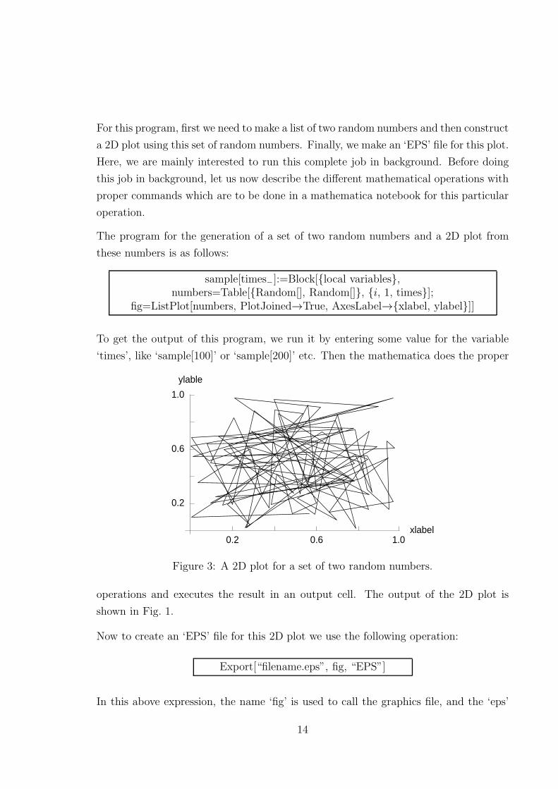
The program for the generation of a set of two random numbers and a 2D plot from

these numbers is as follows:

sample[times−]:=Block[{local variables},

numbers=Table[{Random[], Random[]}, {i, 1, times}];fig=ListPlot[numbers, PlotJoined→True, AxesLabel→{xlabel, ylabel}]]

To get the output of this program, we run it by entering some value for the variable

‘times’, like ‘sample[100]’ or ‘sample[200]’ etc. Then the mathematica does the proper

0.2 0.6 1.0xlabel

0.2

0.6

1.0

ylable

Figure 3: A 2D plot for a set of two random numbers.

operations and executes the result in an output cell. The output of the 2D plot is

shown in Fig. 1.

Now to create an ‘EPS’ file for this 2D plot we use the following operation:

Export[“filename.eps”, fig, “EPS”]

In this above expression, the name ‘fig’ is used to call the graphics file, and the ‘eps’

14

file is saved by the name ‘filename.eps’ in the present working directory.

Thus we are now clear about all the mathematical operations those are to be done

in a mathematica notebook for the above mentioned program. So now we make our

attention for running this program in background.

In order to run this program in background, first we need to create a batch-file which

is a text file from these mathematica input commands those are written in different

cells of a mathematica notebook. For this purpose, we go through these steps:

(a) Select the cells from the mathematica notebook, and then follow the direction by

clicking on Cell → Cell Properties → Initialization Cell from the menu bar to initialize

the cells.

(b) To generate the batch-file, follow the direction by clicking on File → Save As

Special. . . → Package Format from the menu bar.

Then a dialog box appears for specifying the file name and the location of the

mathematica input file. Here we use the input file for the operation of the mathematica

job.

After these steps, let us suppose, we generate a batch-file named as ‘santanu.m’

for the above mathematica program. Generally the batch-files for this purpose are

specified by using the extension ‘.m’ i.e., like the name as ‘filename.m’. To run this

batch-file ‘santanu.m’ in background, we use the following prescription:

nohup time math < santanu.m > santanu.out &

The file name ‘santanu.out’ is the output file, where all the outputs for the different

operations are available. To get both the input and output lines of the mathematica

notebook, it is necessary to use the following command in the first line of the notebook.

AppendTo[$Echo, “stdout”]

At the end of all these steps, we get the output file ‘santanu.out’ and the graphics

file ‘filename.eps’ in ‘EPS’ format in the present working directory where the batch-file

‘santanu.m’ is run in the background.

5 Parallel Evaluation of Mathematica Programs

Parallelization is a form of computation in which one can perform many operations si-

multaneously. Parallel computation uses multiple processing elements simultaneously

15

to finish a particular job. This is accomplished by breaking the job into independent

parts so that each processing element can execute its part of the algorithm simultane-

ously with the others. The processing elements can be diverse and include resources

such as a single computer with multiple processors, several networked computers, spe-

cialized hardware, or any combination of the above.

In this section, we narrate the basic mechanisms for parallelizing a mathematica

program by running its independent parts in several computers available in the network.

Since all the basic mathematical operations are performed quite nicely in any version of

mathematica, it does not matter even if different versions of mathematica are installed

in different computers those are required for the parallel computing.

5.1 How to Open Mathematica Slaves in Local Computer ?

In parallel computation, different segments of a job are computed simultaneously.

These operations can be performed either in a local computer or in remote computers

available in the network. Separate operations are exhibited in separate mathematica

slaves. In order to emphasize the basic mechanisms, let us now describe the way of

starting a mathematica slave in a local computer. To do this, first we load the following

package in a mathematica notebook.

Needs[“Parallel`Parallel`”]

To enable optional features, then we load the package,

Needs[“Parallel`Commands`”]

Now we can open a mathematica slave in the local computer by using the command,

LaunchSlave[“localhost”, “math -noinit -mathlink”]

Using this command, several mathematica slaves can be started from the master slave.

Now it becomes much more significant if we specify the names of different slaves so

that independent parts of a job can be shared into different slaves appropriately. For

our illustrations, below we give some examples how different slaves can be started with

specific names.

link1=LaunchSlave[“localhost”, “math -noinit -mathlink”]link2=LaunchSlave[“localhost”, “math -noinit -mathlink”]link3=LaunchSlave[“localhost”, “math -noinit -mathlink”]

16

Here link1, link2 and link3 correspond to the three different slaves. The details of these

slaves can be available by using the following command,

TableForm[RemoteEvaluate[{$ProcessorID, $MachineName, $SystemID,$ProcessID, $Version}], TableHeadings→{None,{“ID”, “host”, “OS”,

“process”, “Mathematica Version”}}]

The output of the above command becomes (as an example),

ID host OS process Version1 tcmpibm AIX-Power64 463002 5.0 for IBM AIX Power (64 bit)

(November 26, 2003)2 tcmpibm AIX-Power64 299056 5.0 for IBM AIX Power (64 bit)

(November 26, 2003)3 tcmpibm AIX-Power64 385182 5.0 for IBM AIX Power (64 bit)

(November 26, 2003)

The results shown in this table are for the above three slaves named as link1, link2 and

link3 respectively, where all these slaves are opened from the local computer named

as ‘tcmpibm’ (say). To get the information about the total number of slaves those are

opened, we use the command,

Length[$Slaves]

For this case, the total number of slaves becomes 3.

5.2 How to Open Mathematica Slaves in Remote Computers

Available in Network ?

To start a slave in remote computer, the command ‘ssh’ is used which offers secure

cryptographic authentication and encryption of the communication between the local

and remote computer. Before starting a slave in a remote computer, it is necessary to

check whether ‘ssh’ is properly configured or not, and this can be done by using the

prescription,

ssh remotehost math

For example, if we want to connect a remote computer named as ‘tcmpxeon’, we should

follow the command as,

17

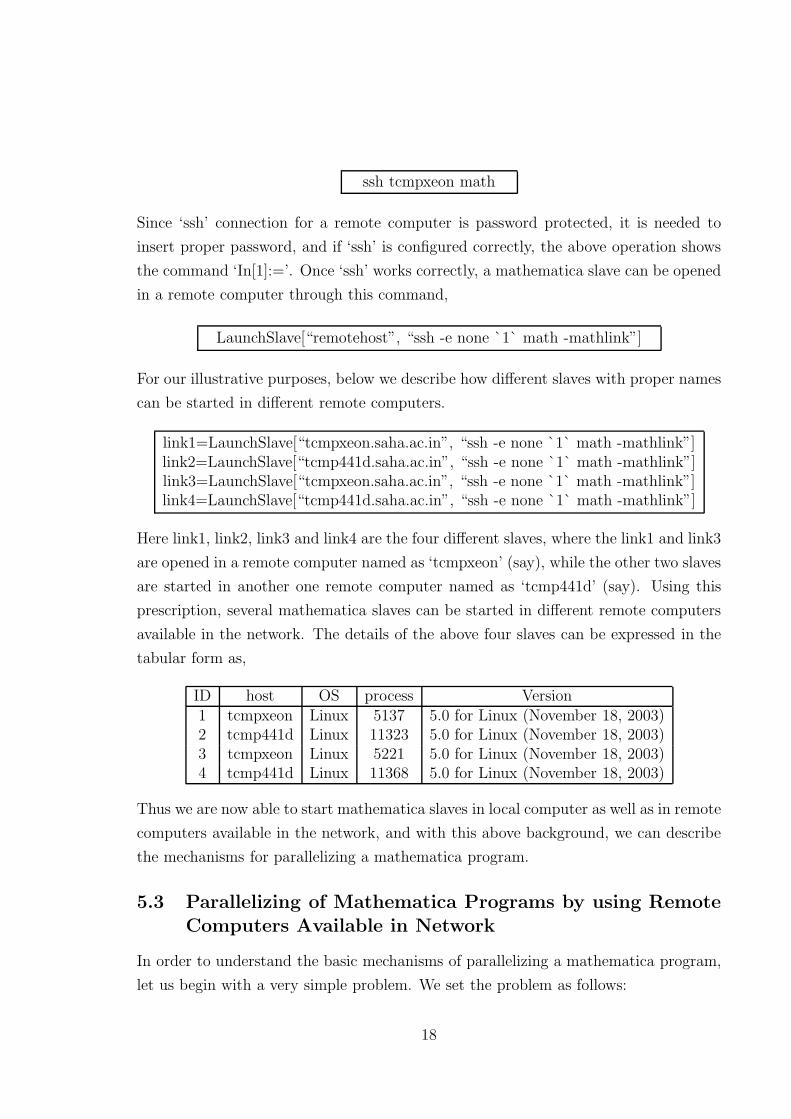
ssh tcmpxeon math

Since ‘ssh’ connection for a remote computer is password protected, it is needed to

insert proper password, and if ‘ssh’ is configured correctly, the above operation shows

the command ‘In[1]:=’. Once ‘ssh’ works correctly, a mathematica slave can be opened

in a remote computer through this command,

LaunchSlave[“remotehost”, “ssh -e none `1` math -mathlink”]

For our illustrative purposes, below we describe how different slaves with proper names

can be started in different remote computers.

link1=LaunchSlave[“tcmpxeon.saha.ac.in”, “ssh -e none `1` math -mathlink”]link2=LaunchSlave[“tcmp441d.saha.ac.in”, “ssh -e none `1` math -mathlink”]link3=LaunchSlave[“tcmpxeon.saha.ac.in”, “ssh -e none `1` math -mathlink”]link4=LaunchSlave[“tcmp441d.saha.ac.in”, “ssh -e none `1` math -mathlink”]

Here link1, link2, link3 and link4 are the four different slaves, where the link1 and link3

are opened in a remote computer named as ‘tcmpxeon’ (say), while the other two slaves

are started in another one remote computer named as ‘tcmp441d’ (say). Using this

prescription, several mathematica slaves can be started in different remote computers

available in the network. The details of the above four slaves can be expressed in the

tabular form as,

ID host OS process Version1 tcmpxeon Linux 5137 5.0 for Linux (November 18, 2003)2 tcmp441d Linux 11323 5.0 for Linux (November 18, 2003)3 tcmpxeon Linux 5221 5.0 for Linux (November 18, 2003)4 tcmp441d Linux 11368 5.0 for Linux (November 18, 2003)

Thus we are now able to start mathematica slaves in local computer as well as in remote

computers available in the network, and with this above background, we can describe

the mechanisms for parallelizing a mathematica program.

5.3 Parallelizing of Mathematica Programs by using Remote

Computers Available in Network

In order to understand the basic mechanisms of parallelizing a mathematica program,

let us begin with a very simple problem. We set the problem as follows:

18

Problem: Construct a square matrix of any order in a local computer and two other

square matrices of the same order with the previous one in two different remote com-

puters. From the local computer, read these two matrices those are constructed in the

two remote computers. Finally, take the product of these three matrices and calculate

the eigenvalues of the product matrix in the local computer.

To solve this problem we proceed through these steps in a mathematica notebook.

Step-1 : For the sake of simplicity, let us first define the names of the three different

computers those are needed to solve this problem. The local computer is named as

‘tcmpibm’, while the names of the other two remote computers are as ‘tcmpxeon’ and

‘tcmp441d’ respectively. Opening a mathematica notebook in the local computer, let

us first load the package for parallelization, and to get the optional features, we load

another one package as mentioned earlier in Section 2. Then we start two mathemat-

ica slaves named as ‘link1’ and ‘link2’ in the two remote computers ‘tcmpxeon’ and

‘tcmp441d’ respectively by using the proper commands as discussed in Section 3.

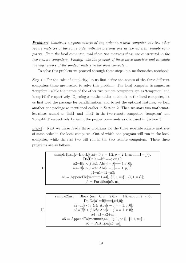
Step-2 : Next we make ready three programs for the three separate square matrices

of same order in the local computer. Out of which one program will run in the local

computer, while the rest two will run in the two remote computers. These three

programs are as follows.

I.

sample1[ns−]:=Block[{esi= 0, t = 1.2, p = 2.1,vacuum1={}},

Do[Do[a1=If[i==j,esi,0];a2=If[i < j && Abs[i − j]== 1, t, 0];a3=If[i > j && Abs[i− j]== 1, p, 0];

a4=a1+a2+a3;a5 = AppendTo[vacuum1,a4], {j, 1, ns}], {i, 1, ns}];

a6 = Partition[a5, ns]]

II.

sample2[ns−]:=Block[{esi= 0, q = 2.6, r = 1.8,vacuum2={}},

Do[Do[a1=If[i==j,esi,0];a2=If[i < j && Abs[i− j]== 1, q, 0];a3=If[i > j && Abs[i − j]== 1, r, 0];

a4=a1+a2+a3;a5 = AppendTo[vacuum2,a4], {j, 1, ns}], {i, 1, ns}];

a6 = Partition[a5, ns]]

19

III.

sample3[ns−]:=Block[{esi= 0, u = 2, v = 3,vacuum3={}},

Do[Do[a1=If[i==j,esi,0];a2=If[i < j && Abs[i − j]== 1, u, 0];a3=If[i > j && Abs[i− j]== 1, v, 0];

a4=a1+a2+a3;a5 = AppendTo[vacuum3,a4], {j, 1, ns}], {i, 1, ns}];

a6 = Partition[a5, ns]]

Since we are quite familiar about the way of writing mathematica programs [1, 6],

we do not describe here the meaning of the different symbols used in the above three

programs further. Thus by using these programs, we can construct three separate

square matrices of order ‘ns’.

Step-3 : We are quite at the end of our complete operation. For the sake of simplicity,

we assume that, the program-I is evaluated in the local computer, while the program-

II and program-III are evaluated in the two remote computers respectively. All these

three programs run simultaneously in three different computers. To understand the

basic mechanisms, let us follow the program.

sample4[ns−]:=Block[{},

ExportEnvironment[“Global`”];mat1 = sample1[ns];

RemoteEvaluate[Export[“data1.dat”, sample2[ns]], link1];RemoteEvaluate[Export[“data2.dat”, sample3[ns]], link2];

mat2 = RemoteEvaluate[ReadList[“data1.dat”, Number, RecordLists→ True],link1];

mat3 = RemoteEvaluate[ReadList[“data2.dat”, Number, RecordLists→ True],link2];

mat4 = mat1.mat2.mat3;Chop[Eigenvalues[mat4]]]

This is the final program. When it runs in the local computer, one matrix called as

‘mat1’ is evaluated in the local computer (3rd line of the program), and the other

two matrices are determined in the remote computers by using the operations given in

the 4th and 5th lines of the program respectively. The 2nd line of the program gives

the command for the transformations of all the symbols and definitions to the remote

computers. After the completion of the operations in remote computers, we call back

these two matrices in the local computer by using the command ‘ReadList’, and store

them in ‘mat2’ and ‘mat3’ respectively. Finally, we take the product of these three

20

matrices and calculate the eigenvalues of the product matrix in the local computer by

using the rest operations of the above program.

The whole operations can be pictorially represented as,

Master slave inlocal computer

tcmpibm

remote computertcmpxeon

Daughter slave in Daughter slave inremote computer

tcmp441d

Figure 4: Schematic representation of parallelization.

At the end of all the operations, we close all the mathematica slaves by using the

following command.

CloseSlaves[ ]

Concluding Remarks

In summary, the basic operations presented in this communication may be quite helpful

for the beginners. Starting from the basic level, in Section 2, we have explored how to

start mathematica, open a mathematica notebook, write a program in mathematica,

etc. Following with this, we have also described the utilities of the local and global

variables those are used for writing programs in mathematica.

Later, in Section 3, we have illustrated the basic mechanisms for the linking of ex-

ternal programs with mathematica notebook. This mathlink operation is an important

part of this article, and it is extremely crucial for doing large numerical computations.

Here we have concentrated the mathlink operation mainly for the XL Fortran 90 source

21

files. But this operation can also be used for any other Fortran source file. In this sec-

tion, we have also illustrated very briefly about the optimization techniques for the

Fortran source files which may help us to run very complicated jobs quite efficiently.

In Section 4, we have addressed in detail how to set up a mathematica batch-file

from a mathematica notebook and run it in the background of a computer. Several

programs are there which can take a considerable amount of time to run. Some may

take few days or even few weeks to complete their analysis. For this reason, it may be

desirable to place such jobs in the background. This is a way of running a program that

allows one to continue working on other tasks (or even log out) while still keeping the

program running. Furthermore, backgrounded jobs are not dependent on our session

remaining open, so even if our computer crashes, the job will continue uninterrupted.

At the end, in Section 5, we have explored the basic mechanisms for parallelizing a

mathematica program by running its independent parts in remote computers available

in the network. By using this parallelization technique, one can enhance the efficiency

of the numerical works, and it helps us to perform all the mathematical operations

within a very short period of time.

Throughout this article, we have focused all the basic operations for the Unix

based operating system only. But all these operations also work very well in any other

supported operating system like Windows, Macintosh, etc.

Acknowledgment

I acknowledge with deep sense of gratitude the illuminating comments and suggestions

I have received from Prof. Sachindra Nath Karmakar during the preparation of this

article.

References

[1] Stephen Wolfram. Mathematica-5.0.

[2] Roman E. Maeder. About Parallel Computing Toolkit. A Wolfram Research Ap-

plication Package.

[3] I. M. Smith. Programming in Fortran 90 : A First Course for Engineers and

Scientists. University of Manchester, UK.

22

[4] Martin Counihan. Fortran 90. University of Southampton.

[5] IBM. XL Fortran for AIX : User’s Guide.

[6] Santanu K. Maiti. A Basic Introduction on Math-Link in Mathematica, Ref.:

arXiv:cs/0603005v3 [cs.MS] 17th October, 2008.

[7] Santanu K. Maiti. How to Run Mathematica Batch-files in Background ?, Ref.:

arXiv:cs/0604088v3 [cs.MS] 17th October, 2008.

[8] Santanu K. Maiti. Parallel Evaluation of Mathematica Programs in Remote Com-

puters Available in Network, Ref.: arXiv:cs/0606023v3 [cs.MS] 17th October, 2008.

23