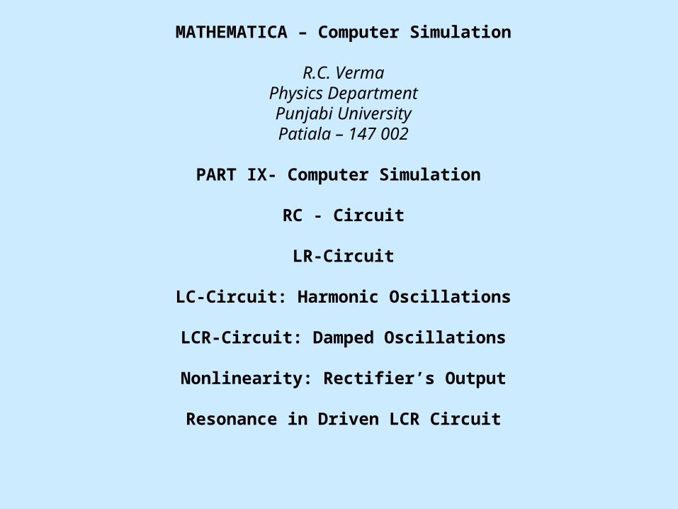
MATHEMATICA – Computer Simulation

R.C. VermaPhysics DepartmentPunjabi UniversityPatiala – 147 002

PART IX- Computer Simulation

RC - Circuit

LR-Circuit

LC-Circuit: Harmonic Oscillations

LCR-Circuit: Damped Oscillations

Nonlinearity: Rectifier’s Output

Resonance in Driven LCR Circuit

Charging and Discharging Capacitor (RC – Circuit)

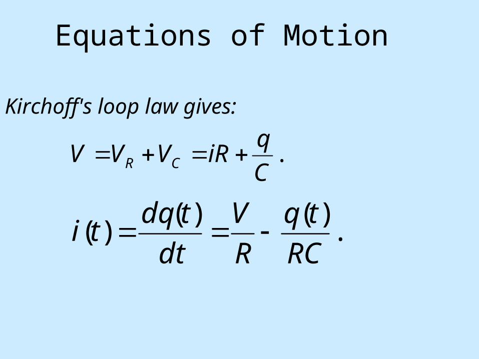
Equations of Motion

Kirchoff's loop law gives:

.

C

qiRVVV CR

.)()(

)(RC

tq

R

V

dt

tdqti

RC- Circuit

Clear["Global`*"]r = 0.85; c = 1.2; (* inputs:- R & C *)v= 0.1; q0=0; (* voltage applied & initial charge *)tmin = 0; tmax = 5;

ndsol = NDSolve[ Join[ {r q'[t]+q[t]/c -v==0}, {q[0]==q0}], q[t], {t, tmin, tmax}

]Plot[ q[t]/.ndsol, {t, tmin, tmax},

PlotLabel->"Charging of a Capacitor", AxesLabel->{"t", "q"} ]

1 2 3 4 5t

0 .02

0 .04

0 .06

0 .08

0 .10

0 .12

q

C harging of a C ap acit or

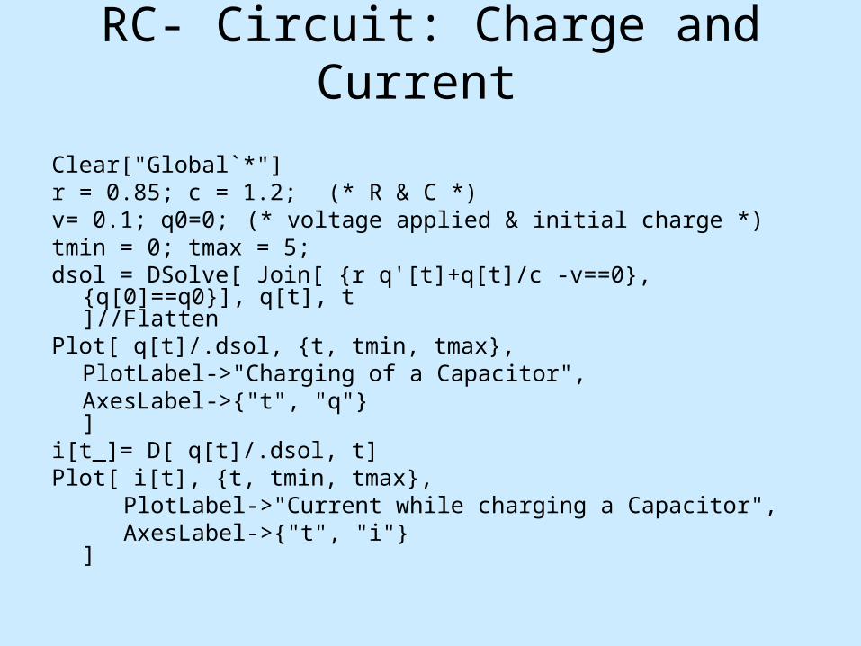
RC- Circuit: Charge and Current

Clear["Global`*"]r = 0.85; c = 1.2; (* R & C *)v= 0.1; q0=0; (* voltage applied & initial charge *)tmin = 0; tmax = 5;dsol = DSolve[ Join[ {r q'[t]+q[t]/c -v==0}, {q[0]==q0}], q[t], t

]//FlattenPlot[ q[t]/.dsol, {t, tmin, tmax}, PlotLabel->"Charging of a Capacitor", AxesLabel->{"t", "q"}

]i[t_]= D[ q[t]/.dsol, t]Plot[ i[t], {t, tmin, tmax}, PlotLabel->"Current while charging a Capacitor",

AxesLabel->{"t", "i"}]

1 2 3 4 5

t

0 .02

0 .04

0 .06

0 .08

0 .10

0 .12

q

C harging of a C ap acit or

{q[t] (-0.980392 t (-0.12+0.12 (0.980392 t)}

0.117647 (0. t-0.980392 (-0.980392 t (-0.12+0.12 (0.980392 t)

1 2 3 4 5t

0 .0 2

0 .0 4

0 .0 6

0 .0 8

0 .1 0

0 .1 2i

C urrent w hile charging a C ap acit or

RC- Circuit: Resistance changes with time

Clear["Global`*"]r=0.85; res[t_]:= r*(1+0.8*t) c = 1.2; (* R & C *)v= 0.1; q0=0; (* voltage applied & initial charge *)tmin = 0; tmax = 8;ndsol = NDSolve[ Join[ {r*q'[t]+q[t]/c -v==0}, {q[0]==q0}], q[t], {t, tmin, tmax}]ndsol1 = NDSolve[ Join[ {res[t]*qv'[t]+qv[t]/c -v==0}, {qv[0]==q0}], qv[t],

{t, tmin, tmax}]i[t_]= D[ q[t]/.ndsol, t]iv[t_]= D[ qv[t]/.ndsol1, t]Plot[ {q[t]/.ndsol, qv[t]/.ndsol1} , {t, tmin, tmax}, PlotLabel->"Charging of a

Capacitor", AxesLabel->{"t", "q"}, PlotStyle-> {Dashing[{}], Dashing[{0.02}]}Plot[ {i[t], iv[t]}, {t, tmin, tmax}, PlotLabel->"Current while charging a Capacitor",

AxesLabel->{"t", "i"}, PlotStyle-> {Dashing[{}], Dashing[{0.02}]} ]

2 4 6 8t

0 .0 2

0 .0 4

0 .0 6

0 .0 8

0 .1 0

0 .1 2

q

C harging of a C ap acit or

2 4 6 8t

0 .01

0 .02

0 .03

0 .04

0 .05

0 .06

i

C urrent w hile charging a C ap acit or

Growth of Current in RL – Circuit

Recalling that voltage across the inductor L is given by

.dt

diLVL

Kirchoff's loop law:

.

i

L

R

L

V

dt

di

RL- Circuit

Clear["Global`*"]r = 0.85; ind = 1.2; (* R & L *)v= 0.1; i0=0; (* voltage applied & initial current *)tmin = 0; tmax = 5;dsol = DSolve[ Join[ { i'[t]+i[t]*r/ind -v/ind==0}, {i[0]==i0}], i[t], t]//FlattenPlot[ i[t]/.dsol, {t, tmin, tmax}, PlotLabel->"Current in RL Circuit",

AxesLabel->{"t", "i"}]

{i[t] (-0.708333 t (-0.117647+0.117647 (0.708333 t)}

1 2 3 4 5t

0 .0 2

0 .0 4

0 .0 6

0 .0 8

0 .1 0

i

C urrent in R L C ircuit

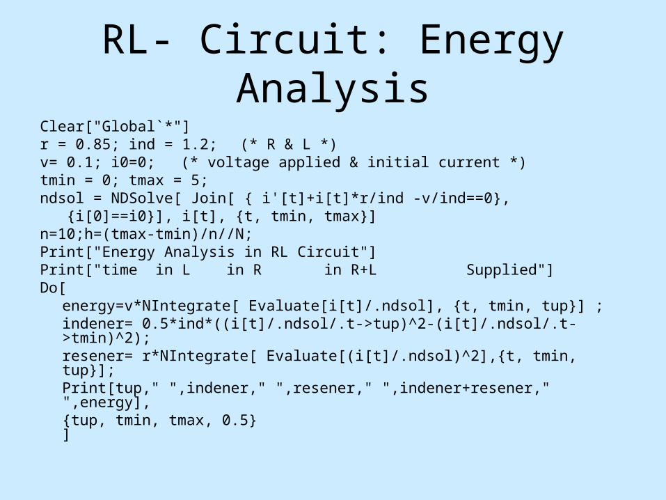
RL- Circuit: Energy AnalysisClear["Global`*"]r = 0.85; ind = 1.2; (* R & L *)v= 0.1; i0=0; (* voltage applied & initial current *)tmin = 0; tmax = 5;ndsol = NDSolve[ Join[ { i'[t]+i[t]*r/ind -v/ind==0}, {i[0]==i0}], i[t], {t, tmin, tmax}]n=10;h=(tmax-tmin)/n//N;Print["Energy Analysis in RL Circuit"]Print["time in L in R in R+L Supplied"]Do[

energy=v*NIntegrate[ Evaluate[i[t]/.ndsol], {t, tmin, tup}] ;indener= 0.5*ind*((i[t]/.ndsol/.t->tup)^2-(i[t]/.ndsol/.t->tmin)^2);resener= r*NIntegrate[ Evaluate[(i[t]/.ndsol)^2],{t, tmin, tup}];Print[tup," ",indener," ",resener," ",indener+resener," ",energy],

{tup, tmin, tmax, 0.5}]

Energy Analysis in RL Circuittime in L in R in R+L Supplied0. {0.} {0} {0.} {0}0.5 {0.000738671} {0.000190181} {0.000928853} {0.000928852}1. {0.00213918} {0.00119587} {0.00333505} {0.00333505}1.5 {0.00355641} {0.00322156} {0.00677798} {0.00677798}2. {0.00476491} {0.00618354} {0.0109484} {0.0109484}2.5 {0.00571834} {0.00991114} {0.0156295} {0.0156295}3. {0.00643929} {0.0142295} {0.0206688} {0.0206688}3.5 {0.00697079} {0.0189887} {0.0259595} {0.0259595}4. {0.00735635} {0.0240704} {0.0314267} {0.0314267}4.5 {0.00763311} {0.0293846} {0.0370177} {0.0370177}5. {0.00783039} {0.0348652} {0.0426956} {0.0426956}

RL- Circuit: Resistance changes with time

Clear["Global`*"]r = 0.85; ind = 1.2; (* R & L *)v= 0.1; i0=0; (* voltage applied & initial current *)tmin = 0; tmax = 5;res[t_]:= r*(1+0.8 *t)ndsol = NDSolve[ Join[ { i'[t]+i[t]*r/ind -v/ind==0}, {i[0]==i0}], i[t], {t, tmin, tmax}]//Flattenndsol1 = NDSolve[ Join[ { iv'[t]+iv[t]*res[t]/ind -v/ind==0}, {iv[0]==i0}], iv[t], {t, tmin, tmax}]//FlattenPlot[ {i[t]/.ndsol, iv[t]/.ndsol1}, {t, tmin, tmax}, PlotLabel->"Current in RL Circuit", AxesLabel->{"t", "i"}, PlotStyle->{Dashing[{}],Dashing[{0.02}] }]

1 2 3 4 5t

0 .0 2

0 .0 4

0 .0 6

0 .0 8

0 .1 0

i

C urrent in R L C ircuit

LC- Circuit: Harmonic Oscillations

,,,dt

diLVCVq

dt

dqi

which can be expressed as

q

LCdt

qd 12

2

natural angular frequency of the oscillations,

,1

LC

LC- CircuitClear["Global`*"]ind = 1.2;cap=0.85; (* L C *)i0=1.0;q0=1.0; (* initial conditions *)tmin = 0; tmax = 15;dsol = DSolve[ Join[ { q''[t]+ q[t]/(ind*cap)==0}, {q[0]==q0, q'[0]==i0}], q[t], t]//Flatten//Chopi[t_]=D[ q[t]/.dsol, t]Plot[ {q[t]/.dsol, i[t]}, {t, tmin, tmax}, PlotLabel->"Oscillations in LC-Circuit", AxesLabel-

>{"t", "q"}, PlotStyle->{Dashing[{}], Dashing[{0.01}]}, PlotPoints->50

]Print[" ----------------------------"]Print[" Energy Analysis in LC Circuit"]Print[" in L in C total"]Print[" ----------------------------"]Do[ indener = 0.5*ind*i[t]^2; capener = 0.5*(q[t]/.dsol)^2/cap; Print[ indener," ",capener," ",indener+capener], {t, tmin, tmax, 1.0}

] Print[" ----------------------------"]

{q[t]1. Cos[0.990148 t]+1.00995 Sin[0.990148 t]}

2 4 6 8 1 0 1 2 1 4t

1 .0

0 .5

0 .5

1 .0

q

O scillat ions in LC C ircuit

Energy Analysis in LC Circuit in L in C total ----------------------------

0.6 0.588235 1.188240.046806 1.14143 1.188241.02406 0.164176 1.188240.799067 0.389168 1.188240.0009749 1.18726 1.188240.861487 0.326748 1.188240.974354 0.213881 1.188240.0239661 1.16427 1.188240.667892 0.520343 1.188241.10552 0.0827127 1.188240.113112 1.07512 1.188240.465737 0.722498 1.188241.17735 0.0108826 1.188240.258068 0.930167 1.188240.278478 0.909757 1.18824

1.18151 0.00672513 1.18824 ----------------------------

LCR-Circuit: Damped Oscillations

Equations governing the system then become,

,,,

iR

dt

diLVCVq

dt

dqi

which are combined to yield

.

12

2

dt

dqR

C

q

Ldt

qd

LCR- CircuitClear["Global`*"]ind = 1.2;cap=0.85;res=0.5; (* L C R *)i0=1.0;q0=1.0; (* initial conditions *)tmin = 0; tmax = 15;dsol = DSolve[ Join[ { q''[t]+q'[t]*res/ind+ q[t]/(ind*cap)==0}, {q[0]==q0, q'[0]==i0}], q[t], t ]//Flatten i[t_]=D[ q[t]/.dsol, t] Plot[ {q[t]/.dsol, i[t]}, {t, tmin, tmax}, PlotLabel->"Damped Oscillations in LCR-Circuit", AxesLabel->{"t", "q & i"}, PlotStyle->{Dashing[{}], Dashing[{0.01}]}, PlotPoints->50 ]

{q[t](-0.208333 t (1. Cos[0.967982 t]+1.2483 Sin[0.967982 t])}

2 4 6 8 10 12 14t

1 .0

0 .5

0 .5

1 .0

q & i

D amp ed O scillat ions in LC R C ircuit

LCR- Circuit: time-varying resistance

Clear["Global`*"]ind = 1.2;cap=0.85;res=0.02; (* L C R *)r[t_]:= res*(1+0.3*t^2)i0=1.0;q0=1.0; (* initial conditions *)tmin = 0; tmax = 25;dsolv = NDSolve[ Join[ { q''[t]+q'[t]*r[t]/ind+ q[t]/(ind*cap)==0}, {q[0]==q0, q'[0]==i0}], q[t], {t, tmin, tmax}]//Flattenp1= Plot[ {q[t]/.dsolv}, {t, tmin, tmax},

PlotLabel->"Time Varying R in LCR-Circuit: ", AxesLabel->{"t", "q"}, PlotStyle->{ Dashing[{0.01}]}, PlotPoints->50 ];

dsol = NDSolve[ Join[ { q''[t]+q'[t]*res/ind+ q[t]/(ind*cap)==0}, {q[0]==q0, q'[0]==i0}], q[t], {t, tmin, tmax}]//Flattenp2 = Plot[ {q[t]/.dsol}, {t, tmin, tmax}, AxesLabel->{"t", "q"},

PlotPoints->50 ];Show[p1, p2]

Nonlinearity : Rectifier's Output

• Clear["Global`*"]• w= 2.0;• tmin = 0; tmax = 6;• eps = 1.1;• v[t_]:= Sin[w*t]• Plot[ v[t], {t, tmin, tmax},• PlotLabel -> "Input Signal", AxesLabel->{"t", "v"}]• Plot[ v[t]+eps*v[t]^2, {t, tmin, tmax},• PlotLabel -> "Output Signal", AxesLabel->{"t", "v"}]

1 2 3 4 5 6t

1 .0

0 .5

0 .5

1 .0

v

Inp ut Signal

1 2 3 4 5 6t

0 .5

1 .0

1 .5

2 .0

v

O utp ut Signal

Nonlinear Circuit

r = 100.0;k = 1.39*10^(-23);t = 300;q = 1.6*10^(-19);i0 = 10^(-10);v1= 15.0;FindRoot[{(v1-v2)/r == i0*(E^(q*v2/(k*t))-1)}, {v2, 0.5}]v1= 15.1;FindRoot[{(v1-v2)/r == i0*(E^(q*v2/(k*t))-1)}, {v2, 0.5}]

{v2 -> 0.549695}{v2 -> 0.549874}

RVVI /)( 21

)1( /0

2 kTqVeII

Familiar I-V equation for Diode, q is electron charge, I0 is leakage current (~10-10 amp)

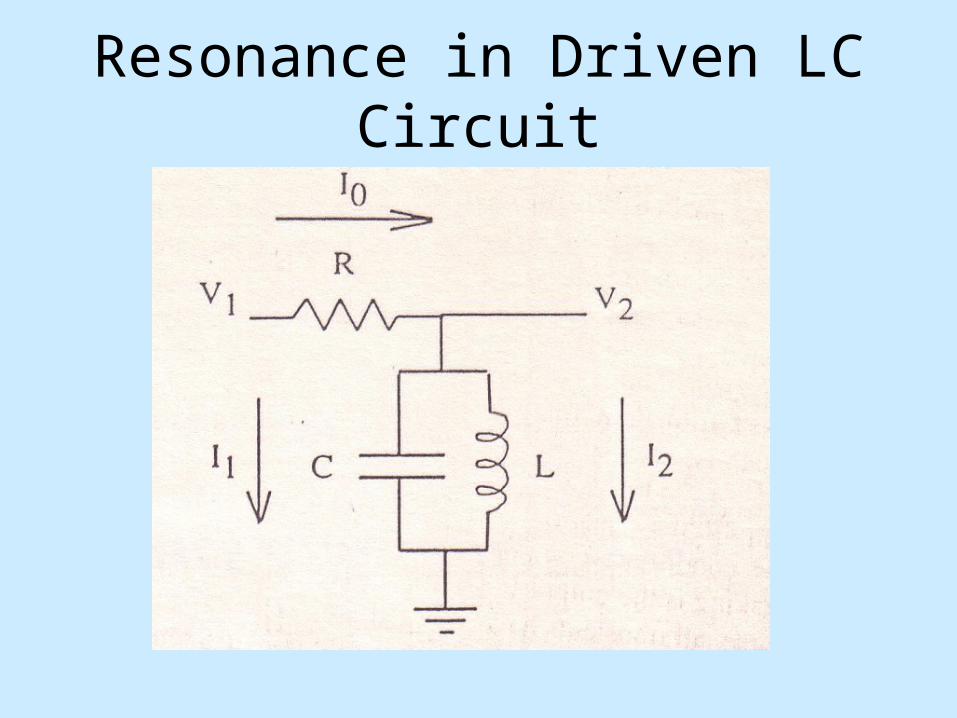
Resonance in Driven LC Circuit

Eqns. for time dependent Voltage

22

12

210

021 )())()((

Vdt

dIL

Idt

dVC

III

RtItVtV

Steady State for w

Clear["Global`*"]dsol = Solve[{v1*E^(I w t)-v2*E^(I w t)== i0*r*E^(I w t), i0== i1+i2, c*D[v2*E^(I w t), t]==i1*E^(I w t), l*D[i2*E^(I w t), t]==v2*E^(I w t)},

{v2, i0, i1, i2}]Simplify[dsol]c = 10^(-6);l = 10^(-3);v1=1;Plot[Release[Table[Abs[v2]/.dsol[[1]]/.r->10^n, {n,2,4,0.5}]], {w, 20000, 40000}, PlotRange -> {0,1}]

v1 I l v1 w c l v1 w {{i0 -> -- + -----------------------------, i1 -> -----------------------------, r r (-r + I l w (-1 - I c r w)) -r + I l w (-1 - I c r w) v1 -I l v1 w i2 -> -(------------------------- ), v2 -> ---------------------------- }} -r + I l w (-1 - I c r w) -r + I l w (-1 - I c r w)

Thank You