Mathematical Analysis and Numerical Simulation of Electromigration by Jon Arthur Wilkening B.S. (University of Arizona) 1996 A dissertation submitted in partial satisfaction of the requirements for the degree of Doctor of Philosophy in Mathematics in the GRADUATE DIVISION of the UNIVERSITY of CALIFORNIA at BERKELEY Committee in charge: Professor James A. Sethian, Chair Professor Alexandre J. Chorin Professor Andrew K. Packard Spring 2002
Transcript
Mathematical Analysis and Numerical Simulation of Electromigration
by
Jon Arthur Wilkening
B.S. (University of Arizona) 1996
A dissertation submitted in partial satisfaction of the
requirements for the degree of
Doctor of Philosophy
in
Mathematics
in the
GRADUATE DIVISION
of the
UNIVERSITY of CALIFORNIA at BERKELEY
Committee in charge:
Professor James A. Sethian, ChairProfessor Alexandre J. ChorinProfessor Andrew K. Packard
Spring 2002
Mathematical Analysis and Numerical Simulation of Electromigration
Copyright 2002
by
Jon Arthur Wilkening
1
Abstract
Mathematical Analysis and Numerical Simulation of Electromigration
by
Jon Arthur Wilkening
Doctor of Philosophy in Mathematics
University of California at BERKELEY
Professor James A. Sethian, Chair
We develop a model for mass transport phenomena in microelectronic interconnect
lines, study its mathematical properties, and present a number of new numerical methods
which are useful for simulating the process.
The central focus of the work is an investigation of the well-posedness of the grain
boundary diffusion problem. The equation is stiff and non-local and depends on gradients
of the stress components σij , which contain singularities near corners and grain boundary
junctions. We show how to recast the problem as an ODE on a Hilbert space, and prove that
the non-selfadjoint compact operator involved has a real, non-negative spectrum and a set
of eigenfunctions which is dense in L2(Γ), where Γ is the grain boundary network. We show
that in the limit of an infinite interconnect line, the eigenfunctions are sines and cosines,
and through numerical studies show that for a finite line, in spite of non-orthogonality, the
eigenfunctions form a well conditioned basis for L2(Γ). We develop a numerical method
for simulating the evolution process, and obtain results which are self-consistent under
mesh-refinement and make physical sense.
The main tool we develop for solving the elasticity equations with high resolution
near corners and grain boundary junctions is a singularity capturing extension of the First
Order System Least Squares finite element method. We call the method XFOSLS. The
method is designed for polygonal domains with corners, cracks, and interface junctions,
and can handle complicated jump discontinuities along interfaces while maintaining smooth
displacement and stress fields (which may be unbounded near corners) within each region of
the domain. Several self-similar (not necessarily singular) solutions may be adjoined to each
2
corner or junction, and the supports of the extra basis functions may overlap one another.
We also present a number of new techniques for computing bases of self-similar
solutions for corners and interface junctions. These include an algorithm for removing rank
deficiency from the basis matrix at isolated parameter values, a stabilization algorithm for
removing near linear dependency from the power solutions corresponding to characteristic
exponents which are clustered together, and a new theorem about Keldysh chains which
leads to an algorithm for computing associated functions. Several examples are given which
illustrate the techniques.
Professor James A. SethianDissertation Committee Chair
1.1 Left: Scanning Electron Micrograph picture of a multilevel CMOS integratedcircuit with the intermatallic dielectric etched away. (From Solid State Elec-tronic Devices, Streetman/Banerjee [73]). Right: Schematic view of the com-ponents of a microchip. (From Microchip Fabrication, Van Zant [81]). . . . 2
2.2 Arbitrary local orientation of grain boundary segment determines tangentialand normal directions, left and right grain labels, etc. . . . . . . . . . . . . 18
2.3 Meaning of the separation function g. The regions between dashed and solidlines in the top two pictures represent material which has been added orremoved from each grain during the transport process. The actual displace-ments would be much smaller than those shown here. . . . . . . . . . . . . 19
2.4 Compatibility condition on the separation function g at a triple point. . . 20
2.5 Volume and surface fluxes J and Js give the number of atoms crossing areaand line elements dA and dl when dotted with them. In 2D simulationswe are still modeling 3D objects, so the units are (cm2s)−1 and (cm s)−1,respectively. . . . . . . . . . . . . . . . . . . . . . . . . . . . . . . . . . . . 21
2.6 The continuity equation and void growth equation are a consequence of massconservation. . . . . . . . . . . . . . . . . . . . . . . . . . . . . . . . . . . . 22
2.7 Left: high resolution TEM microscope image of a large tilt angle grain bound-ary in a gold thin film. (From Electronic Thin Film Science for ElectricalEngineers and Materials Scientists, Tu/Mayer/Feldman [77]). Right: graingrowth occurs when more atoms flow into a region of the grain boundarythan out. . . . . . . . . . . . . . . . . . . . . . . . . . . . . . . . . . . . . . 24
2.8 Two systems in thermal and diffusive contact must have equal chemical po-tentials. . . . . . . . . . . . . . . . . . . . . . . . . . . . . . . . . . . . . . . 25
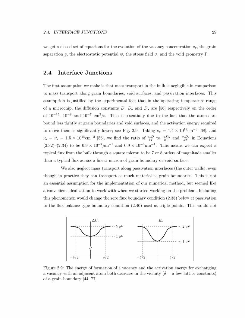
2.9 The energy of formation of a vacancy and the activation energy for ex-changing a vacancy with an adjacent atom both decrease in the vicinity(δ = a few lattice constants) of a grain boundary [44, 77]. . . . . . . . . . . 29
2.10 The electric field can lead to a flux imbalance at a triple point which mustbe compensated by stress gradients to satisfy mass conservation. . . . . . . 31
vi
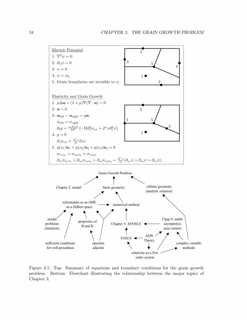
3.1 Top: Summary of equations and boundary conditions for the grain growthproblem. Bottom: Flowchart illustrating the relationship between the majortopics of Chapter 3. . . . . . . . . . . . . . . . . . . . . . . . . . . . . . . . 34
3.2 The force per unit area exerted by the positive side on the negative side of asurface with normal n is given by σn . . . . . . . . . . . . . . . . . . . . . 39
3.3 The geometry and boundary conditions for the grain growth problem on aninfinite strip. . . . . . . . . . . . . . . . . . . . . . . . . . . . . . . . . . . . 45
3.4 A plot of C(ω) for h = 1 and κ = 1.15, 1.4, 2.0, 3.0. Note that C(ω) divergesin the incompressible (κ→ 1), long wavelength (ω → 0) limit. . . . . . . . 47
3.5 A plot of the dissipation rate C(ω)ω2 for h = 1 and κ = 1.001, 1.01, 1.1, 2.0.Note that even though C(ω) is not monotonic for κ < 2, C(ω)ω2 is monotonicfor ω ≥ 0. The envelope of the graphs approaches 3
3.6 The geometry and boundary conditions of a finite interconnect line with asingle horizontal grain boundary running through its center. . . . . . . . . 55
3.7 A contour plot of σ22(x, y) corresponding to the steady state solution. Notethat σ22 decreases linearly along the grain boundary to balance the constantelectromigration force that arises due to the linearly increasing potential ψ.(s22 is σ22). . . . . . . . . . . . . . . . . . . . . . . . . . . . . . . . . . . . 56
3.8 It suffices to be able to solve gt = −LSg for g ∈ L2MZ . . . . . . . . . . . . . 57
3.9 A plot of the absolute value of f(z) = 1z (e−z − 1) + 1 along the rays z = s,
z = 1+2i√5s, z = 1+7i√
50s, z = is. The maximum principle together with the
graph along z = ±is gives that |f(z)| < 1.5 for all z in the right half plane. 633.10 Each grain is triangulated separately, leading to an unstructured mesh with
duplicate nodes along grain boundaries. This particular mesh corresponds toa mesh parameter h = 0.05 for an interconnect line of unit height and lengthtwo. . . . . . . . . . . . . . . . . . . . . . . . . . . . . . . . . . . . . . . . . 65
3.11 Sparsity pattern for several matrices. (a) The stiffness matrix A which resultsfrom the least squares finite element method for the mesh in Fig. 3.10. (b)The lower triangle of the matrix A obtained from A using symamd to re-orderthe rows and columns. (c) The Cholesky factorization L, where LLT = A. 67
3.12 The first 14 basis functions ei for the space of separations. Each of the threespecial basis functions shown consists of a power solution piece (of the formRecrλ) and a quadratic piece. The exponents involved here are λ = 0.680and 1.709± 0.604 i. . . . . . . . . . . . . . . . . . . . . . . . . . . . . . . . 68
3.13 Evolution of the normal stress η along the grain boundary for the two meshesat t = 0.005, 0.01, 0.02, 0.04, 0.08, 0.16, 0.32. . . . . . . . . . . . . . . . . . . 75
3.14 Evolution of the separation function g along the grain boundary for the twomeshes at t = 0.005, 0.01, 0.02, 0.04, 0.08, 0.16, 0.32. . . . . . . . . . . . . . 76
3.15 Log-Log plot of eigenvalues λj of K vs. index j. The red and blue curves(a) and (b) show the eigenvalues obtained from the coarse and fine meshes,respectively. The green line (c) is a plot of 0.32j−3, which appears to be theasymptotic limit of the spectrum of K for large j. In the bottom plot, wezoom in on a portion of the top plot. . . . . . . . . . . . . . . . . . . . . . 77
vii
3.16 The first 4 eigenfunctions ϕk of K. Note that the eigenfunctions are smooth,oscillatory, and satisfy zero flux boundary conditions at the endpoints. Thescales are arbitrary (normalized as vectors in Rn rather than in L2). . . . . 78
3.17 The first 4 eigenfunctions φk of K. Note that they are smooth, oscillatory,and satisfy the zero displacement boundary conditions at the endpoints. Thescales are arbitrary (normalized as vectors in Rn rather than in L2). . . . . 79
3.18 The first 3 eigenfunctions ϕ∗k of K∗ along with the corresponding (rescaled)eigenfunctions φk of K. A surprising discovery: K = K∗. The coefficients inthe expansion η =
∑akϕk are determined by ak =
∫ηϕ∗k, so these functions
can be thought of as linear functionals. . . . . . . . . . . . . . . . . . . . . 80
3.20 Arbitrary local orientation of grain boundary segment determines tangentialand normal directions, left and right grain labels, etc. . . . . . . . . . . . . 82
3.21 Each grain is triangulated separately, leading to an unstructured mesh withduplicate nodes along grain boundaries and triple nodes at triple junctions.Offsets have been added to the nodes of each grain here to show the finiteelement connectivity of the spacially coincident grain boundary nodes tothe interior nodes. This particular mesh corresponds to a mesh parameterh = 0.06 for an interconnect line which fits in a rectangle of length 4.25 andheight 2. . . . . . . . . . . . . . . . . . . . . . . . . . . . . . . . . . . . . . 86
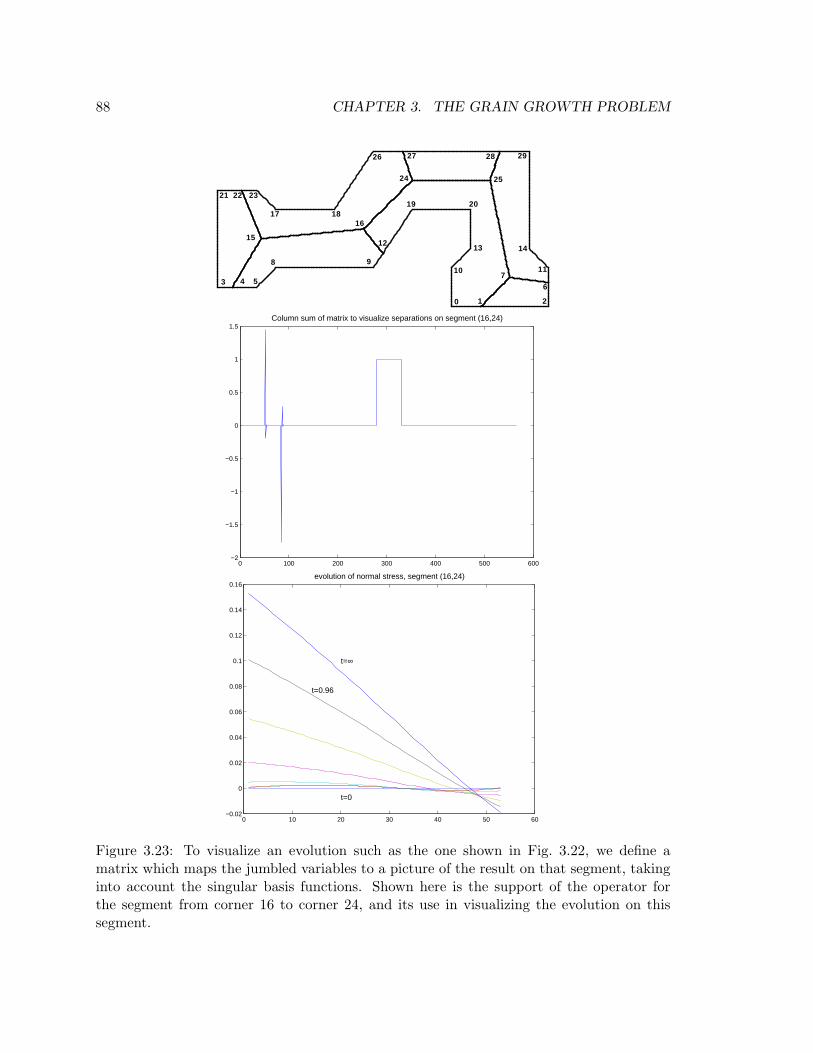
3.22 The normal stress variables are ordered by taking the grain boundary end-points and triple points first, and then sweeping through the interior of eachgrain boundary segment. The separation variables include the special basisfunctions used to capture asymptotic behavior near corners and triple junc-tions. These basis functions all have zero normal stress on grain boundaries.The apparently large amplitude of the coefficients on these special basis func-tions is an artifact of how they are normalized in the code. This evolutionwill be further discussed in Section 3.4.8. . . . . . . . . . . . . . . . . . . . 87
3.23 To visualize an evolution such as the one shown in Fig. 3.22, we define amatrix which maps the jumbled variables to a picture of the result on thatsegment, taking into account the singular basis functions. Shown here is thesupport of the operator for the segment from corner 16 to corner 24, and itsuse in visualizing the evolution on this segment. . . . . . . . . . . . . . . . 88
3.24 Compatibility condition on the separation function g at a triple point. . . . 89
3.25 Top: Corners and grain boundary junctions are numbered arbitrarily. Mid-dle: The electrostatic potential ψ satisfies Laplace’s equation with Dirichletboundary conditions at the ends and Neumann boundary conditions on theside walls. We use standard variational finite elements with quadratic ele-ments on the mesh used in the elasticity problem to determine ψ along Γ.Bottom: A plot of the number of degrees of freedom that affect the variablesat a given vertex or edge node. In this simulation, 101 extra basis functionsnear corners and junctions are used to capture asymptotic behavior. . . . . 93
viii
3.26 The evolution of g and η on the segment from junction 16 to junction 24 inFig. 3.25. Times shown are t = .03, .06, .12, .24, .48, .96,∞. The plot was ob-tained by applying the visualization operator for this segment (c.f. Fig. 3.23)to the evolution of the variables shown in Fig. 3.22 on Page 87. . . . . . . 94
3.27 The evolution of g and η on the segment from junction 24 to junction 27at t = .03, .06, .12, .24, .48, .96,∞. Note that initially material leaves thissegment, but the flux of mass at the triple point changes sign around t = .045and ultimately the grains separate along this segment. . . . . . . . . . . . 95
3.28 The evolution of g and η on the segment from junction 25 to junction 7at t = .03, .06, .12, .24, .48, .96,∞. Note that unlike the simple horizontalgeometry, the steady state normal stress η = P ∗(−ψ
∣∣Γ) does not vary lin-
early along grain boundary segments. Also note that g develops an infiniteslope at the endpoints due to singularities. Asymptotically, g ∼
∑cir
λi
with λ(7)i ∈ 0, .799, .886 and λ
(25)i ∈ 0, .725, .951. The other stress
components diverge at the ends (like rλ−1 with λ(7) ∈ .799, .886 andλ(25) ∈ .725, .951), but η remains well behaved. . . . . . . . . . . . . . . 96
3.29 Top: Magnified view of the steady state separation g(x), obtained by plottingx + Cu+(x) and x + Cu−(x) with x along the grain boundary. Bottom:Contour plot of the magnitude of the displacements in each grain, togetherwith streamlines tangent to the displacement vector field. Note that materialis transported from the left end of the interconnect line to the right, causingthe grains to move toward each other (g < 0) on the left side and to separate(g > 0) on the right. . . . . . . . . . . . . . . . . . . . . . . . . . . . . . . . 97
3.30 Contour plots of the steady state values of p = 12(σ11 + σ22), µ−1σijεij =
κ−12 p2 + γ2 + τ2, and (γ2 + τ2)
12 . Note that the left and right ends of the
line are generally in a state of tension and compression, respectively, dueto the transport of mass from left to right. Also note that the stresses arelargest where the grains have separated the most, and at re-entrant cornersand grain boundary junctions where they have singularities. . . . . . . . . 98
3.31 Contour plots of the steady state values of (u2+v2)12 , p, τ , and κ−1
2 p2+γ2+τ2
for a grain boundary network with two connected components. On eachcomponent, material has been transported from left to right until the gradientof σnn balances the electromigration force. The break in the network in themiddle of the line acts as a barrier to limit the effective length of the line.Large stresses develop at the gb–wall junctions where the centermost grain isbeing pushed to the right by grain growth on its left and grain annihilationon its right, but is clamped in place at the top and bottom. The net result ofthe barrier, however, is to reduce the distance over which the stress gradientmust balance the electromigration force, and hence the maximum stress issmaller than it would be for a single component grain boundary network onan interconnect line of this length. . . . . . . . . . . . . . . . . . . . . . . . 99
ix
3.32 Each grain is traversed counterclockwise with unit inward normal n. Thecontribution of a particular grain boundary segment to the total elastic en-ergy E =
∑Ek contains precisely one term from the left grain and one term
4.1 The angles ωk divide R2 into several regions Ωk. . . . . . . . . . . . . . . . 108
4.2 Geometry of Example 9: a corner with Dirichlet boundary conditions im-posed along one ray and traction boundary conditions imposed along theother. Recall (page 39) that u‖ = u · t, u⊥ = u · n, σs = t · σn, σ⊥ = n · σn,and T = σn. . . . . . . . . . . . . . . . . . . . . . . . . . . . . . . . . . . . 111
4.3 Top: Radial and angular dependence of the six components u, v, p, q, γ, τof a nontrivial solution of the form wj(r, θ) = rλ+tjφj(θ) (λ = 0.6157) to theincompressible Lame equations with Dirichlet boundary conditions on eachray of the region (−π/6 < θ < 7π/6). Bottom: A 3D plot of the variable τ . 117
4.4 Contour plots of the zero level sets of the real and imaginary parts of ∆(λ)along with the contours generated by the clustering algorithm for findingroots. Top: wall–gb–wall geometry with ω0 = 90, ω1 = 173, ω2 = 270.Bottom: triple grain boundary junction with ω0 = −174, ω1 = −51, ω2 =45, ω3 = 186. Note that some clusters contain multiple (or nearly multiple)roots which must be resolved accurately. . . . . . . . . . . . . . . . . . . . 126
4.5 Algorithm for finding all Keldysh chains at λ0. . . . . . . . . . . . . . . . . 132
4.6 Top: Contour plot of the zero level sets of the real and imaginary parts of∆(λ) for a T-shaped triple grain boundary junction with angles ω0 = −90,ω1 = 90, ω2 = 180, ω3 = 270 and elastic constant κ = 1.6. There is a zeroof order 6 at λ = 0, a simple zero at λ = 0.6298473, a zero of order 4 at λ = 1,and a zero of order 3 at λ = 2. At λ = 0, the kernel of A(λ) has dimension 3and there are 3 linearly independent Keldysh chains of length two. At λ = 1and λ = 2, the dimension of the kernel is respectively 4 and 3, so there areno associated functions at these values of λ. Bottom: When the geometry isperturbed, (ω1 → 80 here), the root at λ = 0 remains unchanged (includingKeldysh chain structure), the root at λ = 1 splits into a simple root at λ ≈ 1and a threefold root at λ = 1, and the root at λ = 2 splits into three simpleroots, one equal to 2 and the others complex. This example illustrates manyof the complicated possibilities that can occur. . . . . . . . . . . . . . . . . 133
4.7 Contour plot of the zero level sets of the real and imaginary parts of ∆(λ) for acheckerboard pattern of two materials with Lame coefficients µ1 = 1, µ2 = 10,κ1 = 1, κ2 = 2.4. Note the four nearly identical roots near λ = 2.8± .96i. . 136
5.1 Each grain is triangulated separately, leading to an unstructured mesh withduplicate nodes along grain boundaries. This particular mesh correspondsto a mesh parameter h = 0.033 for an interconnect line of unit height andlength two. . . . . . . . . . . . . . . . . . . . . . . . . . . . . . . . . . . . . 142
x
5.2 The fringe region of a regular hexagonal mesh corresponding to fringe radius=3.Nodes within a radius of 3h inclusive are “near” nodes. Triangles with somenear nodes and some far nodes are “fringe” triangles. If several singularitiesexist at the corner, each may have a different fringe radius. . . . . . . . . . 144
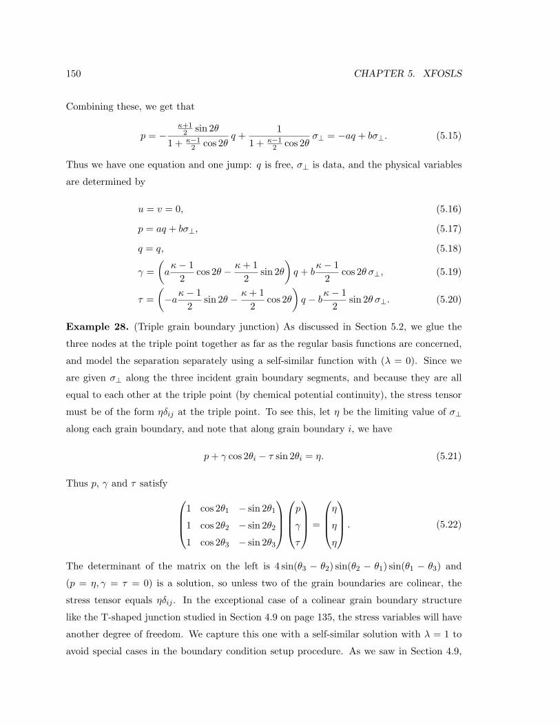
5.3 Typical entry in the boundary condition file. . . . . . . . . . . . . . . . . . 1485.4 Geometry of a junction where a grain boundary meets a wall. . . . . . . . 1495.5 Comparison of γ for the steady state solution to the grain growth problem
near a corner using XFOSLS (top) and standard Galerkin finite elements(bottom). The roughness of the contours in the top plot is an artifact of vi-sualization, where linear interpolation is being used to compute contour lineson the four sub-triangles joining the six nodes of each trianglular element;see also Figure 5.6. . . . . . . . . . . . . . . . . . . . . . . . . . . . . . . . 156
5.6 A contour plot showing the behavior of the solution γ from Figure 5.5 near agrain boundary junction with a wall. Points were uniformly sampled withinthe triangles of the mesh shown. . . . . . . . . . . . . . . . . . . . . . . . . 157
5.7 The solution obtained via the Galerkin method with a much finer grid stillexhibits undesirable behavior near the corner, where the stress obtained viaLagrange multipliers differs significantly from the stress obtained by differ-entiating the displacements. . . . . . . . . . . . . . . . . . . . . . . . . . . 158
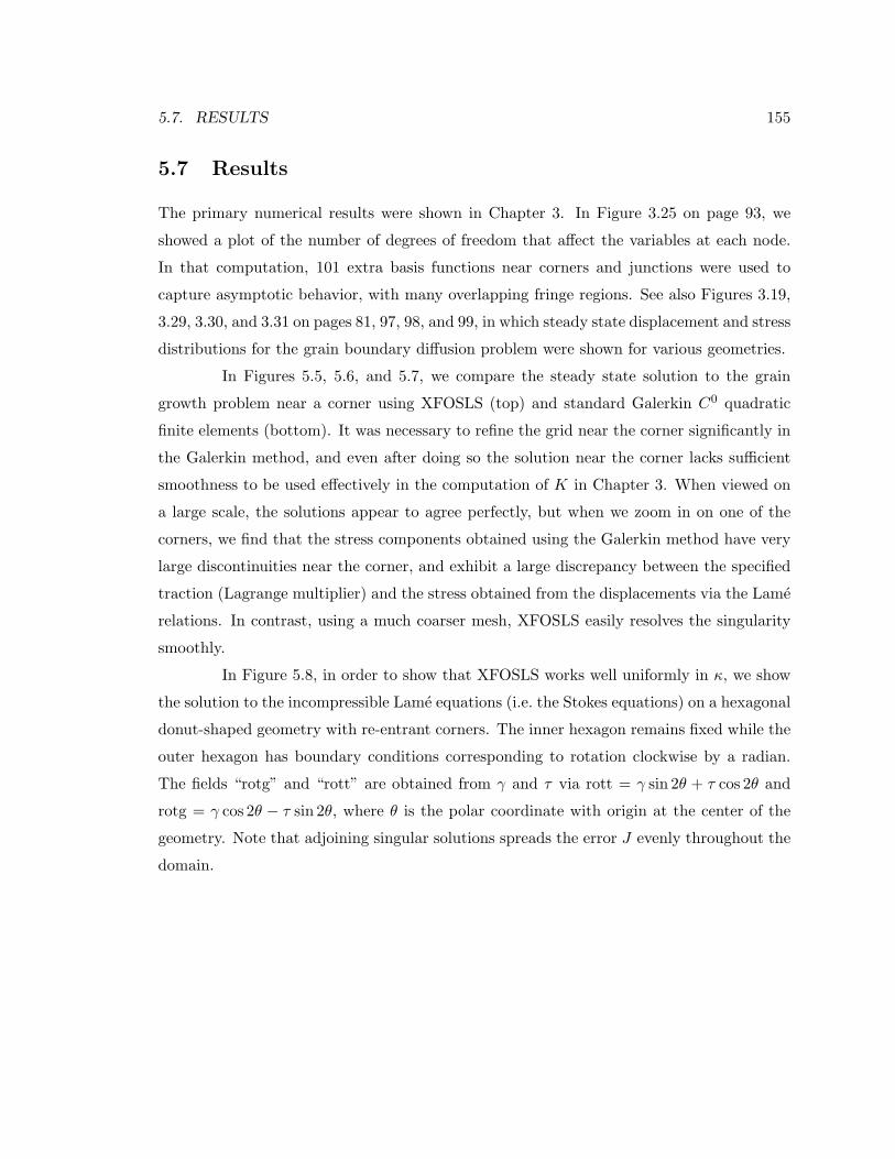
5.8 The solution of the Lame equations with κ = 1 on a hexagonal geometry.Here the inner hexagon remains fixed while the outer hexagon has boundaryconditions corresponding to rotation clockwise by a radian. . . . . . . . . . 159
xi
Acknowledgements
I am very grateful to my dissertation committee, James Sethian, Alexandre Chorin,
and Andrew Packard. Thank you for tolerating my tendency to wait until the last possible
minute to finish things.
I owe special thanks to Len Borucki for all the time and energy he put into working
on the electromigration problem with Jamie and myself during his extended visits to LBL
over the past several years. Len, it has been a pleasure working with you.
My thanks to G. I. Barenblatt for many useful conversations, and for offering a
unique and insightful perspective (both mathematical and historical) on many occasions. I
would also like to thank the many wonderful professors I have taken classes with and got-
ten to know over the years, especially James Sethian, Alexandre Chorin, G. I. Barenblatt,
Ole Hald, Jim Demmel, John Strain, Craig Evans, Michael Christ, William Arveson, Alan
Weinstein, Hendrik Lenstra, James Colliander, Charles Pugh, Alistair Sinclair, Doug Pick-
rell, William Conway, Johann Rafelski, Charles Falco, Donald Huffman, Eugene Commins,
Steven Louie, and Eyvind Wichmann. They have been excellent role models as scientists
and mathematicians.
I have been very fortunate to have the opportunity to work in the mathematics
group at the Lawrence Berkeley National Laboratory. I would especially like to thank Valerie
Heatlie for all her kindness and support. She is without doubt the anchor which binds the
group together socially. Thanks for everything, Val. I would also like to thank David
Adalsteinsson, Ravi Malladi, Anton Kast, Raz Kupferman, Andreas Wiegmann, Sergey
Fomel, Alex Vladimirsky, Alina Chertock, Maria Garzon, Mayya Tokman and Thomas
Deschamps, my recent office mates Alek Shestakov, Dror Givon, and Mike Campbell, and
my fellow students Kevin Lin, Eugene Ingerman, Chris Cameron, Masha Kourkina, Panos
Stinis, Pavel Okunev, Theresa Chow, and Helen Shvets.
I’d like to thank my good friends Kenley Jung, Charles Holton, Joe Fendel and
Kurt Schneider for all the cut-throat poker and monopoly nights, Kevin Lin for braving
several physics courses with me, Darren Kessner for making my first year of graduate school
bearable, and Steve, Rachel, Dell, Anna R., Super Dave, Eric, Abby, Polly and Helen for
being partners in crime at the swimming pool.
I was supported from 1997 through 2001 by a Department of Energy Computa-
tional Science Graduate Student Fellowship. This fantastic program helped connect me to
xii
the world of scientific computing, and I am very grateful to have had the opportunity to be
a part of the program. I very much enjoyed my practicum experience in the T7 and CNLS
divisions at Los Alamos in the summer of 1999. I would particularly like to thank Pieter
Swart, Dave Moulton, Joel Dendy, Mac Hyman, and Antti Pihlaja for making this visit so
enjoyable.
Finally, I get to thank my advisor, James Sethian, for being my friend and mentor,
for being optimistic in the face of difficulties, for being tough on me when I get off track,
for keeping things in perspective and helping me do the same, and for being an exceptional
applied mathematician whom I will always respect and admire. Thank you Jamie.
And to Anna, Mom, Dad, Tom, Katie, Mike, Linda, Louis, Ali and Jason, what
can I say? You guys are the greatest, and I love you dearly.
1
Chapter 1
Introduction
A microelectronic circuit consists of a silicon substrate with doped regions which
function as circuit elements (transistors, diodes, resistors, and capacitors), metal lines and
vias (interconnects) which connect the circuit elements together, intermetallic dielectric
material which keeps the interconnects in place and insulated from each other, various
oxide layers and diffusion barriers which are primarily needed in the manufacturing stage
to control the doping process and keep the aluminum from diffusing into the silicon, and
passivation to keep all the components in place and protected [73, 81]. See Figure 1.1.
A typical interconnect line might be an alloy of Al-0.5%Cu, have dimensions of
0.5 × 0.5 × 300 microns, and carry a current density of 20 mA/µm2. As electrons flow
through the line, they are scattered by imperfections in the crystal lattice of the metal
and impart momentum to the ion cores. This ”electron wind” force is stronger than the
opposing direct force of the electric field, so ions are transported in the same direction as
the flow of electrons. This process is known as electromigration, and is a dominant failure
mechanism in microelectronic devices.
Grain boundaries, void surfaces, and passivation interfaces are fast diffusion paths
along which the diffusion constant is typically 7-8 orders of magnitude higher than in the
grains; therefore, most of the mass transport occurs at these locations. The inhomogeneous
redistribution of atoms leads to the development of stresses in the line. Stress gradients
along grain boundaries and surface tension at void surfaces both contribute to the flux of
atoms, usually opposing the electromigration term and increasing the lifetime of the line.
Significant residual stresses left over from thermal contraction during the manufacturing
process also affect the formation of voids and the transport of atoms.
2 CHAPTER 1. INTRODUCTION
Figure 1.1: Left: Scanning Electron Micrograph picture of a multilevel CMOS integratedcircuit with the intermatallic dielectric etched away. (From Solid State Electronic Devices,Streetman/Banerjee [73]). Right: Schematic view of the components of a microchip. (FromMicrochip Fabrication, Van Zant [81]).
1.1 Literature Survey: Modeling
A good reference on electromigration is the review article by Ho and Kwok [38]. The
concept of the “electron wind” force was formulated by Fiks (1959) and by Huntington and
Grone (1961) [40]. In his experimental work in the 70’s, Blech [7] studied the behavior of thin
films of aluminum and Titanium-Nickel when large currents were passed through them, and
demonstrated the phenomenon of the existence of a threshold current density below which
no damage occurs, which varies inversely with the stripe length. Shortly thereafter, Blech
and Herring [8] offered the explanation that stress gradients were developing along grain
boundaries in the sample to counter the electron wind force, but could only be sustained up
to a critical threshold. Once this threshold was reached, there was no physical mechanism
to stop the transport of material, and the stripe was eroded at one end and formed hillocks
at the other. Herring is best known for his work in the theory of of chemical potentials of
atoms at free surfaces due to surface tension, and along grain boundaries due to stresses [37].
The growth of grain boundary voids in copper wires under stress was studied experimentally
by Hull and Rimmer in 1959 [39].
1.2. LITERATURE SURVEY: NUMERICS 3
Recent theoretical models attempt to explain the role of various combinations of
electromigration, stress gradients, diffusion, temperature, anisotropy, surface tension, and
hillock formation on the mass transport of atoms in the bulk grains, along void surfaces,
along grain boundaries, and at passivation interfaces. Noteworthy theoretical papers that
we are familiar with are the paper of Mullins [56], Korhonen et. al. [47], Sarychev et. al. [68],
Kirchheim [42], and Bower/Craft [9]. The Mullins paper presents a nice overview of mass
transport along surfaces and grain boundaries, and discusses Cobble creep and grain bound-
ary grooving. The papers [68] and [42] are primarily interested in electromigration, stress
driven diffusion, and vacancy generation in the grains, and [47] focuses on electromigration
and grain boundary diffusion. The latter three papers use a statistical argument about the
orientation of the grain boundaries in order to model the stress as a scalar variable instead
of a tensor; one should keep in mind, however, that for any particular sample, the grain
boundaries have a specific geometry, and singularities can occur in the stress field which get
ignored with this simplifying assumption. In [64], the authors attempt to give a quantum
mechanical explanation of the electron wind force experienced by an adatom at the surface
of a current-carrying metal. There is no universal agreement in the electromigration com-
munity on exactly how all the phenomena fit together, especially at junctions where grain
boundaries meet voids or other grain boundaries, and the process of void nucleation is far
from being understood. It is fairly well established, however, that high current densities
together with gradients in chemical potential drive mass transport, which is enough to build
computational models of varying degrees of complexity.
1.2 Literature Survey: Numerics
There have been several numerical simulations of void evolution which take surface diffusion
and electromigration (but not stress) into account. In [69], a boundary element method
is used to follow the evolution of a void in an infinite domain with a constant current
boundary condition at infinity. They investigate the stability of the void shape and speed
of propogation as a function of void size. In [52] and [2], level set methods [70] are employed
to track void evolution for a finite geometry. The former uses the immersed interface method
[51] to compute the electrostatic potentials, and the latter uses black box multigrid [28].
Both suffer from serious timestep limitations due to a CFL condition from surface diffusion,
and neither uses an accurate enough electrostatic solver to compute two derivatives of
4 CHAPTER 1. INTRODUCTION
the electrostatic potential along the void boundary. Both exhibit grid effects. In [6], the
self-similar pinchoff problem for axisymmetric surface diffusion is studied, in which they
introduce a very nice implicit finite difference method which deals effectively with the CFL
problems encountered in the previously mentioned papers. None of these papers includes
the effect of stress or the transport of atoms along grain boundaries or in the bulk.
The most comprehensive computational models with which we are familiar are de-
scribed in several papers by Bower, Craft, Fridline and collaborators; see, for example, [9]
and [33]. They use an advancing front algorithm to generate a sequence of adaptive, evolv-
ing finite element meshes, and have studied grain growth, void evolution, hillock formation,
and grain boundary sliding for possibly anisotropic materials responding to stress, sur-
face tension, thermal expansion, and electromigration. They use some clever semi-implicit
techniques to overcome timestep limitations due to the stiffness of the equations.
1.3 The Grain Growth Problem
In the present work, we focus attention on the grain growth problem with a network of grain
boundaries but no voids. We are particularly interested in the effect of singularities in the
stress field near corners and triple points on the solution, and on questions of well-posedness
of the equations and boundary conditions.
In the limiting case of an interconnect line of infinite length with a single grain
boundary running through its center, we show that it is possible to write down an explicit
formula for the solution by using methods of analytic function theory in planar elasticity.
This formula is useful in understanding the similarities and differences between the grain
growth problem and two well understood parabolic equations, namely ut = uxx (the heat
equation) and ut = −uxxxx (the linearized surface diffusion equation). It provides useful
insight into the nature of the diffusion process involved, and offers reassurance that the
high frequency eigenfunctions for a finite geometry will be almost orthogonal, which is the
one thing we are unable to prove rigorously in our study of the well-posedness of the grain
boundary diffusion problem.
There are several difficulties that make the grain growth problem on a finite domain
with corners and triple points interesting. First, there is the basic numerical challenge
that the equations are stiff, and depend on taking two derivatives of the stress tensor
σij , which itself is a sensitive function of the grain boundary separation g (the jump in
1.3. THE GRAIN GROWTH PROBLEM 5
normal component of displacement across a grain boundary). Second, for most functions g,
the corresponding σ will contain singularities near corners and grain boundary junctions,
which are amplified when derivatives are taken. Since some of the boundary conditions are
expressed in terms of derivatives of the stress components at these points, it is essential that
we understand the precise nature of the singularities there. We will see that the components
of the stress field that enter into the equations and boundary conditions remain finite and
well-behaved near these corners even though the stress tensor as a whole becomes singular.
Third, both the equations and boundary conditions are non-local due to the fact that the
flux depends on g through σ. Flux type boundary conditions constrain the stress field σ at
grain boundary endpoints and junctions, which impose global constraints on the evolution
of g, and are not easy to enforce directly. Stated differently, the rate of growth at a point
on the grain boundary and the boundary conditions which arise as a consequence of mass
conservation and chemical potential continuity at an endpoint or triple point depend on the
current state of the entire system rather than on derivatives of g at that point. One has
to be careful that such constraints on g are compatible with the evolution equation. Using
well understood model problems as a guide, we know that for some problems (such as the
heat equation), it is not possible to specify both Dirichlet and flux boundary conditions
at a boundary. For other problems (such as ut = −uxxxx), obtaining a unique solution
requires that two boundary conditions such as these be specified. Therefore it is important
to investigate the possibility that we have included too many boundary conditions on our
“wish list” of physical properties we would like to hold true. In our analysis, it will turn
out that the grain boundary diffusion problem requires both Dirichlet and flux boundary
conditions, so the physical considerations of Chapter 2 lead to a mathematically well-posed
evolution problem.
The key idea that allows us to handle these difficulties is the reformulation of
the problem as an ordinary differential equation on a Hilbert space. The question of well-
posedness becomes a question of the nature of the spectrum and eigenspaces of a compact
(but non-self-adjoint) operator, and the problem of computing the grain growth evolution
with all the correct boundary conditions enforced becomes a matter of developing a ma-
chinery for computing this operator numerically. Through numerical computations, we
discovered a property of the operator that led us to a proof that the spectrum is real and
non-negative and that the eigenfunctions are dense in L2(Γ), where Γ is the grain boundary
network. Our numerical work also shows that although these eigenfunctions are not orthog-
6 CHAPTER 1. INTRODUCTION
onal, they form a well conditioned basis for L2(Γ) because the high frequency eigenfunctions
are nearly orthogonal to one another. Together with the exact solution we derived for the
infinite interconnect line, this provides strong evidence that the grain boundary diffusion
problem is well-posed.
From a programming perspective, just being able to solve and visualize the solution
to the heat equation on a network of line segments poses a challenging book-keeping problem
due to the lack of a natural ordering of the nodes. But the grain boundary diffusion problem
is considerably more complicated than the heat equation. We must keep track of two levels
of finite element structures which can readily communicate with each other, namely a large
finite element space on which the two dimensional Poisson and Lame equations are solved,
and a small finite element space of grain boundary separations and normal stresses defined
on an essentially one dimensional network of line segments. A considerable amount of
effort was required to design appropriate data structures and algorithms capable of coping
with the complications of jump discontinuities across grain boundaries, singular behavior
of the stress field near corners and junctions, and non-trivial compatibility constraints in
the boundary conditions.
1.4 Stable Asymptotics Near Corners
In Chapter 4, we develop a method of computing stable asymptotics for the solution of
the elastic equations (or any other Agmon-Douglis-Nirenberg elliptic system) near corners.
The problem of understanding the asymptotic behavior of solutions of elliptic systems near
corners in the domain is a well developed subject, and a good deal has been written about
it. Asymptotic solutions to the Laplace equation near a corner of the form rπ/ω sinω (ω is
the opening angle), and the characteristic r−1/2 behavior of the stress field near a crack
tip in the Lame equations, have been understood since the 1930’s and 1950’s, respectively.
The work of Kondratiev, Mazya, Plamenevskij and others in the 1960’s made extensive use
of transform methods to prove isomorphism theorems which characterize the asymptotic
nature of solutions of general elliptic systems in Rn near angular points in the domain; see
the papers [45, 54], the review articles [46, 63], and the books [36, 24] for further details.
These results are appealing mathematically, but are difficult to work with in practice due
to the technical nature of the spaces and the non-constructive description of the results.
Many papers have been written analyzing special cases and equations; for the biharmonic
1.4. STABLE ASYMPTOTICS NEAR CORNERS 7
equation, see [45, 36]; for the Lame system, see [35, 67].
For problems in the plane, the asymptotics near a corner can typically be deter-
mined by solving a generalized eigenvalue problem for an ordinary differential equation.
This has led to a number of computational methods in which this eigenproblem is solved
numerically (with finite elements, for example) in order to determine the characteristic ex-
ponents and angular functions; see [50, 60]. The paper [21] by Costabel and Dauge offers a
nice improvement, in that it gives a constructive description of the singularities for a general
Agmon-Douglis-Nirenberg elliptic system in the plane without recourse to an extraneous
ODE. It becomes possible to solve for the characteristic exponents and angular functions
semi-analytically (only the exponents are inexact), and thus to much higher accuracy for
less computation. They use their method in [23] for non-isotropic linear elasticity. We have
taken their method as a point of departure, and have simplified and solved some of the
technicalities that prevent it from working in special cases. Specifically, we present a new
algorithm for removing rank deficiency from the analytic basis matrix and and show how
to handle multiple or tightly clustered roots of the characteristic determinant ∆(λ) when
finding the critical exponents.
Costabel and Dauge also wrote a paper [22] on stable representations of the asymp-
totics of the solutions, but these representations seem to be of little practical use due to
the fact that they are given in the form of Cauchy integrals with integrands obtained by
existence theorems from the theory of several complex variables; this hides many of the
difficulties of dealing with crossings and branchings of the roots and offers little help in
computations, but is still of theoretical interest. The problem of stability will be further
explained in Chapter 4, but for the present purposes, it means that the most natural choice
of basis functions becomes linearly dependent at certain critical angles of the corner, and
as a result, the coefficients with respect to this basis blow up near these angles.
We present a new algorithm for choosing a different basis for clusters of self-similar
solutions which does not become linearly dependent at the critical angle. We also present
a new theorem about Keldysh chains which leads to an algorithm for computing associated
functions and understanding the structure of the power solutions simply by knowing the
boundary condition matrix A(λ) and its first few derivatives at a critical value of λ. We
have found that our stabilization procedure has the nice feature that at a nearly critical
angle of the geometry, it will give nearly the same power solution basis as the Keldysh chain
procedure at exactly the critical angle. This stabilization process is essential for employing
8 CHAPTER 1. INTRODUCTION
self-similar basis functions in the finite element computations of Chapter 3 due to the fact
that clustered characteristic exponents frequently arise in triple point geometries, and the
corresponding non-stabilized basis functions tend to be highly linearly dependent, leading
to ill-conditioned stiffness matrices if nothing is done for stability.
1.5 Some Pitfalls: How Did We Get Here?
In our initial attempts at solving the grain growth problem, we used variational finite ele-
ments to solve for the normal stresses along grain boundaries given the separation function
g, which is the jump in normal component of displacement. The components of stress σij
are obtained from the displacements ui via the relations
where λ and µ are constants. Because the evolution equation (Eqn. (1.6) below) relates the
rate of change of g to components of σ along the grain boundary, we want the stress field
to be continuous throughout the domain (with a well defined value at each node). By (1.1),
this requires that the displacements be continuously differentiable within each grain and
satisfy special compatibility conditions along the grain boundary. For a horizontal grain
boundary, for example, the conditions
u+1 = u−1 , u+
2 = u−2 + g (1.2)
along the grain boundary imply that
∂xu+1 = ∂xu
−1 , ∂xu
+2 = ∂xu
−2 + g′. (1.3)
Using (1.1) and (1.3) to express stress continuity in terms of displacements, we find that
σ+22 = σ−22 ⇒ ∂yu
+2 = ∂yu
−2 (⇒ σ+
11 = σ−11) (1.4)
σ+12 = σ−12 ⇒ ∂yu
+1 = ∂yu
−1 − g
′. (1.5)
Our initial approach was to model the displacements with C1 Clough-Tocher finite elements
[10] subject to the above constraints on the ui and their derivatives across grain boundaries.
In the simplest case of a horizontal grain boundary with electromigration turned
off, the grain boundary diffusion problem takes the form
gt = −σ22[g]xx (in interior); g = 0, ∂xσ22 = 0 (at endpoints). (1.6)
1.5. SOME PITFALLS: HOW DID WE GET HERE? 9
Here g 7→ σ22[g]xx is a linear functional which maps a given separation function g defined
on the grain boundary to the second derivative of the corresponding normal stress along
the grain boundary obtained by solving the elasticity equations. We immediately ran into
problems due to the fact that the stress components did not belong to the same spaces as
the displacements, being expressed in terms of derivatives of the displacements. Note that
the natural thing to do for Equation (1.6) in the finite element setting is to multiply by a
test function, integrate the right hand side by parts, and split the left hand side into a finite
difference, possibly using a backward Euler, Crank-Nicholson, or Runge-Kutta scheme. This
doesn’t work when g and σ belong to different spaces. We also ran into difficulties deciding
just what boundary conditions to enforce at the walls and triple junctions — after all,
how does one enforce a global constraint like ∂xσ22 = 0 on g? (We answer this question in
Chapter 3). It was not clear at the time that the desired boundary conditions from a physical
point of view were leading to a mathematically well-posed problem. We also were feeling
uncomfortable about what we should do near corners and triple points where the stress field
could develop singularities, and yet also where we wanted flux conditions enforced, which
are expressed in terms of gradients of the stress field. At this point we abandoned this
approach, having learned a good deal about the obstacles involved in solving the problem.
The need for compatible spaces for the stresses and displacements leads to the
literature on mixed finite element methods, where instead of computing the stresses from
derivatives of the displacements, additional variables are added to the system, and the
stresses are expressed in terms of some combination of the new variables and the dis-
placements. (Sometimes the stress components are the new variables). This reformulation
changes the problem from a minimization problem to a saddle point problem; see the book
[10] by Braess for details. It turns out that the spaces used for stress and displacement
cannot be chosen arbitrarily in this framework, but must satisfy the so called inf-sup or
Babuska-Brezzi condition. These methods were primarily designed for the case of nearly
incompressible elastic materials, and there have been quite a variety of strategies used
to construct optimal methods [10, 72, 41, 31, 32], the last containing a class of methods
known as CBB (Circumventing Babuska-Brezzi condition) methods. Unfortunately, all of
them have some property which makes them unsuitable for solving equation 1.6, such as
discontinuous stresses or displacements.
One interesting way to get around the problem of the stress variables belonging to
the wrong spaces is by choosing standard displacement based C0 finite elements, but using
10 CHAPTER 1. INTRODUCTION
Lagrange multipliers to obtain the stresses along grain boundaries instead of differentiating
the displacements. This is analogous to the standard way of imposing a traction boundary
condition, with a few modifications to make it work for a jump condition along a grain
boundary. This is the approach used by Bower, Craft, Fridline, and their collaborators
(see, e.g. [9, 33]). Their approach seems to work quite well, and they have incorporated
an impressive number of interesting phenomena in their model. The method of Lagrange
multipliers does not give stresses at junctions where grain boundaries meet passivation or
other grain boundaries, and there can be large discrepancies near corners between the stress
obtained via Lagrange multipliers and the stress obtained by differentiating the displace-
ments. It is not clear that singularities near corners and triple points can safely be ignored
in this problem, so we take a different approach in order to focus on these issues.
1.6 Capturing Singularities: XFOSLS
In Chapter 5, we develop a singularity capturing, least squares finite element method for
plane elasticity. One can think of standard displacement based variational finite elements
as a problem of finding the state which minimizes the energy functional. In least squares
finite elements (LSFE), we look for the state which minimizes the residual obtained by
plugging the numerical solution into the PDE. The least squares finite element idea goes
back to 1970 with the papers of Bramble and Schatz [11], [12]. There is a nice paper of Aziz,
Kellogg and Stephens [3] written in 1985 which describes how to apply the least squares
finite element method to an arbitrary Agmon-Douglis-Nirenberg elliptic system; specifically
they show how to weight the residuals for the equations and boundary conditions based on
the ADN indices in order to achieve optimal error bounds on the solution. The primary
drawback of their approach is that it leads to unnecessarily bad condition numbers for
the resulting linear systems — a second order system will result in condition numbers of
order h−4 instead of h−2 for the standard Galerkin method. This drawback was removed
(e.g. [18, 62, 15]) with the realization that if the system is first reduced via the Agmon-
Douglis-Nirenberg reduction process [1] to a first order system, then the condition number
is O(h−2) even for problems like the biharmonic equation where the Galerkin method is
O(h−4). The most active work in this direction has led to the FOSLS (First Order System
Least Squares) methodology of Cai, Manteuffel, McCormick and others, where they have
applied it to general second order systems [15], the Stokes problem [16], the pure traction
1.6. CAPTURING SINGULARITIES: XFOSLS 11
problem of planar elasticity [17], and many other problems.
One benefit of using least squares finite elements instead of the Galerkin method
is that there is no Babuska-Brezzi condition to be satisfied [62]. We are free to choose
the spaces for stress and displacement independently. This means that instead of getting
stresses in a space of derivatives of another space, we can use standard quadratic elements
for both displacement and stresses. This is a huge advantage for the grain growth problem.
The other benefit is that we have an a-posteriori gauge of how accurate the solution is,
because we have minimized a residual instead of an energy. On each element of the mesh,
we have a number which tells how accurately the PDE is satisfied on that element. This
idea is made rigorous by Berndt, Manteuffel and McCormick in [4] and [5].
The primary drawback of the FOSLS method is that it requires H2 regularity in
the solution; if the solution is not in H2, the method may fail to converge. One of the key
features which has made variational finite elements so successful is that only H1 regularity
is necessary. When the domain has re-entrant corners, or a change in boudary condition
type from Dirichlet to traction boundary conditions, there is typically a singularity present
that destroys H2 regularity even when the data is smooth. In the grain growth problem,
there are many such singularities, so something must be done in order to get FOSLS to
work. The approach currently being persued by Manteuffel and McCormick to deal with
this problem is known as FOSLS* [14], but this requires giving up the two benefits that led
us to FOSLS in the first place: that the stresses belong to nice spaces and that there is an
a-posteriori error gauge.
Even in the Galerkin setting, singularities invalidate (or weaken the conclusions of)
convergence and regularity proofs, and can make iterative numerical schemes slow. The idea
of augmenting finite element spaces with appropriate singular functions in order to “capture”
the correct asymptotic behavior near corners is an area of active research in the fracture
mechanics community; see [75] and [25] for a sample of some of the recent work in this field.
In the FOSLS framework, Berndt has developed a method of augmenting the finite element
space near interface junctions for the steady state diffusion problem −∇ · (α∇u) = f ,
where the scalar function α may have large jumps across material interfaces. Once these
singularities have been included in the basis set, only the regular part of the solution (the
part that remains when the singularity is subtracted off) needs to be in H2, and the method
converges.
In fracture mechanics, one is primarily interested in crack growth problems, so
12 CHAPTER 1. INTRODUCTION
the difficulty of finding the singularity exponents for each geometry is not confronted – the
geometry is usually a crack, and the characteristic r1/2 behavior for the displacements at a
crack tip has long been known. They do not attempt to include any further terms in the
asymptotic expansion to improve convergence. Berndt’s implementation is also limited to
a single singular function per interface junction, and because he is solving −∇· (α∇u) = f ,
he does not face the difficulties of branching and crossing roots or degenrate or nearly
degenerate singular basis functions that can occur in more general elliptic systems like
elasticity.
In Chapter 5, we develop an approach to augmenting each corner and interface
junction with an arbitrary number of singular functions. We have adopted the name
XFOSLS for our method, following the terminology used by the developers of the extended
finite element method (XFEM) for crack problems [25]. A single singular function is a
chain (usually of length one) of power solutions. They may include logarithm terms, or
simply be an appropriate linear combination of nearly linearly dependent power solutions
to deal with the stability problem discussed in Chapter 4. Each singular function has a
near region, where it is a solution to the PDE, a fringe region, where it transitions to zero,
and a far region where it is zero. Singular functions with smaller real parts are given larger
supports to give the singularity room to die out and become well approximated by the stan-
dard quadratic basis functions. The beauty of the least squares finite element framework
over the Galerkin framework for adjoining singular functions is that because the singular
functions satisfy the PDE in the near and far regions, only the fringe region is relevant for
computing the inner products in the LSFE setting. Therefore inner products only need to
be computed in regions where the functions are well-behaved, and numerical integration
schemes like Gaussian quadrature are fine. By contrast, to adjoin singular functions in
variational finite elements, special methods must be used to get the integration right, and
it is quite difficult to compute the inner products between two different singular functions.
We compare the solution obtained using XFOSLS to solve the Lame equations near
a corner with Dirichlet boundary conditions on one wall and traction boundary conditions
on the other to the solution obtained using the Galerkin finite element method with a locally
refined mesh. When viewed on a large scale, the solutions appear to agree perfectly, but
when we zoom in on one of the corners, we find that the stress components obtained using
the Galerkin method have very large discontinuities near the corner, and exhibit a large
discrepancy between the stress obtained from the displacements using Eqn. (1.1) and the
1.6. CAPTURING SINGULARITIES: XFOSLS 13
specified traction (Lagrange multiplier). In contrast, using a much coarser mesh, XFOSLS
easily resolves the singularity smoothly. We also use XFOSLS to solve the elastic equations
in the incompressible limit (the method works fine over the entire range of poisson ratio)
on a complicated geometry with re-entrant corners to show the effectiveness of the method
outside of the electromigration problem.
15
Chapter 2
A Model of Mass Transport in
Interconnect Lines
In this chapter, we develop a continuum model of mass transport in the bulk grains,
at void surfaces, and along grain boundaries for an interconnect line in a microelectronic
circuit. A typical interconnect line might be made of an alloy of Al-0.5%Cu and have
a diameter of 0.5µm, which is only 1700 times larger than the nearest neighbor distance
for aluminum, which has an FCC lattice structure with a lattice constant of 4.05A and
a nearest neighbor spacing of 2.86A. These interconnects are beginning to approach the
limit in size where it becomes questionable whether there is an intermediate scaling regime
which is large enough that details of the discrete interactions of the atoms in the lattice
can be neglected, but small enough to be considered small in comparison to the geometry
of the macroscopic sample; nevertheless, we believe a continuum approach is useful for
understanding the process of electromigration.
In Section 2.1, we describe the quasi-static aspects of the problem, namely solving
for the electrostatic potential, stress tensor, and displacement field with the void geometry
frozen in time. We define the separation function (jump in normal component of displace-
ment across a grain boundary), derive appropriate boundary conditions at junctions and
endpoints, and discuss the consequences of having jump discontinuities in the displacement
field along grain boundaries. Although these ideas are implicit in [33, 9], no one has pre-
viously singled out the separation function as a key tool for studying the grain growth
problem.
16 CHAPTER 2. A MODEL OF MASS TRANSPORT IN INTERCONNECT LINES
In Sections 2.2–2.4, we describe the role of mass conservation, chemical potential
continuity and the various driving forces for diffusion on the evolution of vacancies, void
surfaces, and grain growth. Although we will ultimately focus on the grain growth problem
in Chapter 3, it is useful to develop our model of grain boundary diffusion in the context of
the more general problem with voids and vacancies taken into account — parallel treatment
helps develop physical insight (and the phenomena are closely related anyway). We treat
the problem as three dimensional in these sections when there is no essential difference
between the two and three dimensional theory.
2.1 The Setup
2.1.1 The Potential Problem
Consider the interconnect line shown in Figure 2.1. We assume the conductivity of the
metal to be homogeneous, and that grain boundaries do not significantly affect the flow of
electric current in the line. The cathode and anode ends of the line are respectively held
at potentials of ψ = 0 and ψ = ψ0, where ψ0 is chosen (depending on the resistivity of the
metal) to produce an average current density across the line of approximately 106 Amp/cm2.
We take ψ0 to be positive, so that electrons are flowing from left to right in the figure. The
other outer walls of the line are assumed to be insulated, so the electric field E = −∇ψhas no component in the normal direction of these walls. Likewise, we take the voids to
be non-conducting, so the electric field is tangent to void surfaces and Neumann boundary
ψ = 0
grain boundary
e−
network ψ = ψ0
void
void
Figure 2.1: Geometry of an interconnect line.
2.1. THE SETUP 17
conditions hold there as well. In summary, at any given instant in time, we assume a steady
current flows through the line, which is modeled by an electrostatic potential ψ satisfying:
∇2ψ = 0 in interior (even at grain boundaries), (2.1)
ψ = 0, ψ = ψ0 at the ends, (2.2)
∂nψ = 0 at other walls and at void boundaries. (2.3)
We remark that although the geometry of the line changes in time, the timescale on which
a void changes shape is practically infinite in comparison to the time it takes for the current
to find its steady state distribution, which justifies this quasi-steady assumption.
2.1.2 The Elasticity Problem
Each grain is assumed to deform elastically, and to satisfy the Lame equations of linear
elasticity. More general non-isotropic linear relationships between stress and strain can
easily be used instead, but we are satisfied with the Lame and Hooke relations:
Lame: σ = 2µε+ λ tr(ε)I, (2.4)
Hooke: ε =1 + ν
Eσ − ν
Etr(σ)I. (2.5)
Here σ is the stress tensor, εij = 12(∂iuj +∂jui) are the components of the strain tensor, u is
the displacement vector field, tr(·) is the trace operator, µ and λ are the Lame coefficients,
and E and ν are Young’s modulus and the Poisson’s ratio; see [48, 19].
When dealing with problems in the plane, we adopt the convention that u has two
components, that σ and ε are 2 × 2 tensors, and that tr(σ) means σ11 + σ22. For plane
strain, we modify (2.5) to account for the neglected σ33 = ν(σ11 + σ22) term:
Hooke: ε =1 + ν
Eσ − ν(1 + ν)
Etr(σ)I. (plane strain) (2.6)
For plane stress, we modify (2.4) to account for the neglected ε33 = − λλ+2µ(ε11 + ε22) term
by using a different expression for λ in terms of E and ν. It is readily verified from (2.4),
(2.5) and (2.6) that the relationship between λ, µ, E and ν is given by
µ =E
2(1 + ν), ν =
λ
(n− 1)λ+ 2µ, (2.7)
λ =Eν
(1 + ν)[1− (n− 1)ν], E =
µ(nλ+ 2µ)12(n− 1)λ+ µ
, (2.8)
18 CHAPTER 2. A MODEL OF MASS TRANSPORT IN INTERCONNECT LINES
where n = 2 in the plane stress case and n = 3 in the plane strain and 3D cases. It will
also prove useful later to make use of the dimensionless parameter κ, defined by
κ =λ+ 3µλ+ µ
=
3− 4ν plane strain (or 3D),
3−ν1+ν plane stress.
(2.9)
The two dimensional Lame equations (c.f. Sec. 3.1) are to be satisfied in the interior of each
grain:
µ∆u + (λ+ µ)∇(∇ · u) = 0. (2.10)
2.1.3 The Separation Function
At any given instant in time, we are given a separation function g which is defined on
the grain boundary network to be the jump in normal component of displacement across
the grain boundary. For any segment on the grain boundary, we choose an orientation for
the segment arbitrarily, which defines a local arclength parameter s, a tangent vector t
pointing in the direction of increasing s, a right adjacent grain (facing in the t direction), a
left adjacent grain, and a normal vector n pointing from right to left (see Figure 2.2). At a
point x in the interior of such a grain boundary segment, we impose four interface boundary
conditions, two which relate the displacement on the right grain to the displacement on the
left grain, and two which express a local balance of forces:
t · (uleft − uright) = 0, (2.11)
n · (uleft − uright) = g, (2.12)
t · (σleftn− σrightn) = 0, (2.13)
n · (σleftn− σrightn) = 0. (2.14)
t
nleft (+)grain
grainright (−)
Figure 2.2: Arbitrary local orientation of grain boundary segment determines tangentialand normal directions, left and right grain labels, etc.
2.1. THE SETUP 19
Equations (2.11) and (2.14) imply that
t · (σleftt− σrightt) = 0, (2.15)
which may be seen by differentiating (2.11) along the grain boundary and writing (2.14)
and (2.15) in terms of derivatives of uleft and uright. Thus we conclude that all components
of the stress tensor are continuous across grain boundaries.
Choosing the opposite orientation for the grain boundary segment will change the
sign of n and swap the right and left labels, so the sign of g is well defined. Physically, a
positive value of g means that two points that were once adjacent to each other on either
side of the grain boundary in the unstressed reference configuration have separated relative
to each other; the gap (in the deformed configuration) between them is to be interpreted
as being filled in by new material that has been added to the grains at the grain boundary.
The orientation of the lattice structure of the new material aligns partly with one grain
and partily with the other; the details of this are not part of our model. Similarly, a
negative value of g means that adjacent points on the grain boundary in the reference
right grain
left grain
right grain
left grain
balancetractionscorresponding points
n
are glued together
gap is filled in
overlap corresponds tomaterial which has been removed
Figure 2.3: Meaning of the separation function g. The regions between dashed and solidlines in the top two pictures represent material which has been added or removed from eachgrain during the transport process. The actual displacements would be much smaller thanthose shown here.
20 CHAPTER 2. A MODEL OF MASS TRANSPORT IN INTERCONNECT LINES
configuration have passed through each other so that an overlap region has developed near
the grain boundary in the deformed state. The seems a little odd at first thought, but within
the linear elasticity model, it is the natural way to represent the physical phenomenon of
removing material from each grain near the grain boundary in the unstressed state and then
gluing the two resulting surfaces together. The overlapping region is the image of the empty
space left behind in the reference configuration rather than a superposition of material. In
Figure 2.3, the displacements are defined on the rectangles bounded by the solid lines in the
reference configuration; the curved dashed lines represent our mental picture of the grain
growth process we are modeling within the linear elasticity framework, but are not part of
the mathematical description; and the curved solid lines in the stressed state are the images
of the displacements along the dotted lines for each grain.
2.1.4 Further Boundary Conditions
At exterior walls, we assume the passivation to be infinitely rigid, and impose the Dirichlet
boundary conditions u = 0. Void surfaces are assumed to be traction free, so if t and n are
tangent and normal vectors to the void surface at x, then t · σ(x)n = 0 and n · σ(x)n = 0.
The separation g is assumed to go to zero at the walls, as it must since both uleft and uright
approach zero there. There is a basic compatibility condition on g where three (or more)
grain boundary segments meet at a point, namely that if we follow the jump in displacement
from grain to grain (counterclockwise, for example), the net jump must be zero when we
get back to the grain we started with. For example, in Figure 2.4, we would require
g(x1)n1 + g(x2)n2 + g(x3)n3 = 0. (2.16)
n1
n2
n3
x1
x2
(the xi are infinitesimallyclose to the triple point.)
x3
Figure 2.4: Compatibility condition on the separation function g at a triple point.
2.2. MASS CONSERVATION 21
We assume g is continuous on each grain boundary segment and has a limiting value at the
endpoints, but the limit is generally different when approaching a triple point from different
segments, subject to the above condition.
Just as we did when computing the electric field, we treat the elasticity problem
as a quasi-steady phenomenon. Although the void geometry will change with time, the
timescale on which voids change shape is very large in comparison to the time it takes the
grains to find their elastic equilibrium, i.e. the speed of void evolution is slow in comparison
to the speed of sound. Thus we may consider the void geometry frozen when determining
the stresses from the separation function g.
In summary, at any instant in time the state of stress of the system is obtained from
the data g by solving the Lame system (2.10) subject to the interface boundary conditions
(2.11)–(2.14) along grain boundaries, the Dirichlet boundary conditions u = 0 along walls,
and traction free boundary conditions at void surfaces.
2.2 Mass Conservation
So far we have only looked at the static aspects of the problem. The dynamics of mass
transport in interconnect lines is governed by mass conservation and various constitutive
laws governing the flux of atoms. In Sections 2.2 and 2.3 we will develop a 3D model of
mass transport in interconnect lines. At each point in the interior of each grain, there is a
flux vector J with units (cm2s)−1 such that for any area element dA the number of atoms
surface flux
dl
dA δJ
J
Jrepresents
J
volume fluxJ
Js
s
s
Figure 2.5: Volume and surface fluxes J and Js give the number of atoms crossing area andline elements dA and dl when dotted with them. In 2D simulations we are still modeling3D objects, so the units are (cm2s)−1 and (cm s)−1, respectively.
22 CHAPTER 2. A MODEL OF MASS TRANSPORT IN INTERCONNECT LINES
crossing dA per unit time is given by J · dA. At each point on a void or grain boundary
surface (speaking three dimensionally here), we have a surface flux Js (denoted Jb for grain
boundaries) with units (cm s)−1 such that for any line element dl the number of atoms
crossing dl per unit time is given by Js · dl. In order to conform as much as possible to
common practice in the electromigration literature, we represent our fluxes, concentrations,
etc. in the units appropriate for three dimensional objects even though our simulations are
done in two dimensions. We simply give the sample a thickness δ and assume all fields are
independent of the coordinate in the transverse direction.
2.2.1 Vacancy Evolution in the Grains
Mass conservation in the bulk grains is expressed via a continuity equation. At each point
in a grain, there is an atomic concentration c which is related to the vacancy concentration
cv and the lattice concentration clat by
c+ cv = clat. (2.17)
If we integrate the flux over a control volume V (see Figure 2.6) and use the divergence
theorem, we obtain the integral form of mass conservation
∂
∂t
∫∫∫Vc dV = −
∫∫∂V
J · n dA = −∫∫∫
V∇ · J dA, (2.18)
from which the continuity and vacancy evolution equations follows immediately:
∂c
∂t+∇ · J = 0, −∂cv
∂t+∇ · J = 0. (2.19)
J
void surface at time t
void surface at time t + ∆t
vn∆t
S
V
J
Js
Figure 2.6: The continuity equation and void growth equation are a consequence of massconservation.
2.3. DRIVING FORCES FOR DIFFUSION 23
In the vacancy equation, one must keep in mind that J is the atomic flux rather than the
(equal and opposite) vacancy flux.
2.2.2 Void Evolution
At void surfaces (speaking three dimensionally), an accumulation of atoms in a region leads
to growth in the normal direction (see Figure 2.6):
1Ω
∫∫SvndA =
∫∫SJ · n dA−
∫∂S
Js · ns dl =∫∫
SJ · n−∇s · Js dA. (2.20)
Here vn is the normal velocity of the void surface, Ω is the volume of an atom in the lattice,
ns is the outward unit surface normal to ∂S (which is tangent to the surface but normal to
the curve ∂S), ∇s · Js is the surface divergence of Js, n is the unit normal pointing away
from the bulk (into the void), and J · n represents the flow of atoms from the bulk (or
grain boundaries) up to the surface. The differential version of this equation gives the void
growth equation
vn + Ω∇s · Js = ΩJ · n (2.21)
2.2.3 Grain Boundary Evolution
Similarly, if along a grain boundary interface there are more atoms flowing into a region
than out (see Fig. 2.7), then the accumulation of atoms will lead to grain growth (i.e. an
increase in grain separation g), which is expressed by the equation
∂g
∂t+ Ω∇s · Jb = 0. (2.22)
The primary difference here is that we do not include the possibility of atoms flowing from
the bulk onto the grain boundary surface; all the physics we have in this model results in
the flow from the right grain to the grain boundary being equal to the flow from the grain
boundary to the left grain, so the net contribution from the bulk is zero.
2.3 Driving Forces for Diffusion
In the previous section we saw how the vacancy concentration (Eqn. 2.19), void surface
velocity (Eqn. 2.21), and grain separation rate (Eqn. 2.22) depend on the fluxes J, Js, and
Jb. In this section we discuss constitutive laws which express the fluxes in terms of the
geometry and state of the system.
24 CHAPTER 2. A MODEL OF MASS TRANSPORT IN INTERCONNECT LINES
grain
boundary
t = 0
new material
t > 0
g
Jb
Jb
Figure 2.7: Left: high resolution TEM microscope image of a large tilt angle grain boundaryin a gold thin film. (From Electronic Thin Film Science for Electrical Engineers and Ma-terials Scientists, Tu/Mayer/Feldman [77]). Right: grain growth occurs when more atomsflow into a region of the grain boundary than out.
2.3.1 The Einstein-Nernst Relation
The central concept in deriving these constitutive laws is the concept of the chemical po-
tential µ of an atom, which in turn relies on the concept of free energy. Free energy is a
measure of the balance between lowering internal energy and raising entropy. In a gas at
constant volume, for example, a system in contact with a heat reservoir will be at thermal
equilibrium when its Helmholtz free energy F = U − TS is minimized; see [43, 82]. If two
systems of a single chemical species are placed in diffusive contact with each other and
in thermal contact with a heat reservoir, the free energy of the combined system will be
minimized at equilibrium with respect to particle exchange between them. Assuming the
free energy is additive, this means we must have equality of the rates of change of each
system with respect to the number of particles (holding temperature and volume fixed), or
else the free energy could be lowered by moving a particle from one system to the other.
This gives the physical importance of the chemical potential µ, defined as
µ(T, V,N) =(∂F
∂N
)T,V
=(∂G
∂N
)T,p
. (2.23)
2.3. DRIVING FORCES FOR DIFFUSION 25
heat reservoir
µ1 µ2
µ1 = µ2
Figure 2.8: Two systems in thermal and diffusive contact must have equal chemicalpotentials.
Here G = U − TS + pV is the Gibbs free energy, which is frequently useful, and plays the
same role as the Helmholtz free energy in the constant pressure case; see Figure 2.8.
In solid mechanics, if an elastic medium occupies a volume V and we perturb the
boundary ∂V infinitesimally to create virtual displacements δu while keeping the system in
mechanical equilibrium, we obtain the following expression for the work done on the system
by the external forces acting on the boundary (n points outward):
∫∂Vδu · (σn) dA =
∫V∂j (δuiσij) dV =
∫V
0︷ ︸︸ ︷(∂jσij) δui + σij (∂jδui) dV
=∫
Vσij
(∂jδui + ∂iδuj
2
)dV =
∫Vσijδεij dV.
(2.24)
The first law of thermodynamics dU = TdS − pdV for a gas is therefore replaced by
dU = TdS +∫
Vσijdεij dV, (2.25)
and the definition of G becomes G = U − TS −∫V σijεij dV . At each point in the inter-
connect line, we consider a volume V centered at this point which is small compared to the
macroscopic dimensions of the sample but large with respect to the atomic spacing, and
compute a value for the chemical potential for the system contained in this volume using
the above formula for G at constant stress. We assume the value µ so obtained becomes
independent of the volume as the volume shrinks to zero (i.e. there is a limit), and in this
way we obtain a spacially varying intensive variable µ, the chemical potential. If the system
were in its final equilibrium stage, µ would be a constant throughout the system. It is
assumed that when the system is not in equilibrium, the chemical potential is continuous,
and the flux of atoms is proportional to the gradient in chemical potential. This is known
26 CHAPTER 2. A MODEL OF MASS TRANSPORT IN INTERCONNECT LINES
as the Einstein-Nernst relation:
J = −cvDkT∇µ, (in bulk), Js = −νsDs
kT∇sµ, (on void and gb surfaces). (2.26)
Here cv is the vacancy concentration (1/cm3), νs is the number of participating atoms per
unit area (1/cm2), D and Ds are the diffusion constants (cm2/s), and k is Boltzmann’s
constant (erg/K). See [56] for further discussion.
2.3.2 The Chemical Potential at a Surface
In [37], Herring argued that the chemical potential of an atom just beneath a curved surface
has the form
µs = µ0 − γΩ(κ1 + κ2), (2.27)
where µ0 is a constant independent of the curvature, γ is the surface tension (typically
∼ 0.1 erg/cm2), and κ1 and κ2 are the principal curvatures of the surface (positive for a
spherical void); see also [13]. Considering the flat case, we see that µ0 is negative and equal
to the cohesive energy per atom in the lattice, or stated differently, the energy required to
form separated neutral atoms divided by the number of atoms. His argument is based on
determining the change in G by looking at the increase in surface energy of a tiny smooth
hump of volume Ω added to the curved surface; the curvature terms come in due to the fact
that the mean curvature κ1 + κ2 is equal to the rate at which the surface area decreases
as the surface moves normally to itself at unit speed. His analysis was done in the more
general case when γ depends on the orientation of the surface, but it reduces to the above
in the isotropic case we are considering.
2.3.3 The Chemical Potential at a Grain Boundary
A similar argument leads to an expression for the chemical potential of an atom near a
grain boundary (see [8]):
µb = µ0 − Ωσnn. (2.28)
Here Ω is the volume of an atom in the lattice and σnn = n · σn is the normal-normal
component of the stress tensor. This can easily be understood by considering the work
done by the stress field when a layer of atoms is added to the grain boundary: only the top
and bottom walls of a small cylindrical control volume placed perpendicular to the grain
boundary move when the layer is added, and only the normal force acting on these walls
2.3. DRIVING FORCES FOR DIFFUSION 27
does work. If the cross section of the control volume is A and the change in height of the
control volume when the layer is added is δ, then the work done by the normal forces is
σnnAδ. Dividing by the number of participating atoms (Aδ/Ω) gives the desired result.
The constant µ0 is again the cohesive energy per atom in the lattice.
2.3.4 The Chemical Potential in the Bulk
To determine the chemical potential of an atom in the bulk, we assume [42, 68] the ex-
istence of a vacancy relaxation factor f between 0 and 1 (typically between 0.2 and 0.4
for a metal [42]) which has the physical interpretation that fΩ is the change in volume of
any macroscopic volume V of the lattice when a vacancy inside V is filled with an atom.
Assuming the inelastic strain field which is responsible for this volume change is localized
at the filled vacancy location and is spherically symmetric, and assuming the stress field
does not change much when a mere vacancy is filled, we find from Eqn. (2.24) that the work
done by the traction forces acting on the boundary of any such V in the process of filling
the vacancy at x is fΩ tr(σ(x)):∫Vσijδεij dV ≈ σij(x)
∫Vδεij dV = σij(x)
(fΩ
δij3
)= f tr(σ)Ω. (2.29)
Also including the standard entropy term to account for the increased number of config-
urations with a given energy which arise when the number of vacancies increases [77], we
obtain the expression
µ = µ1 − fΩ tr(σ)− kT logcvce
(2.30)
for the chemical potential of an atom in the bulk. Here cv is the vacancy concentration, ce
is the equilibrium vacancy concentration, and µ1 is negative in sign and equal to the energy
of formation of a vacancy in the unstressed state, i.e. the energy required to pluck an atom
out of the middle of the lattice and move it to infinity. If the surrounding atoms did not
adjust their relative positions when a vacancy is formed (which would be the f = 0 case),
we would have µ1 = 2µ0 by a standard “when we sum over the atoms we count each bond
twice” argument. But since there is a considerable amount of relaxation energy involved in
forming a vacancy, µ1 is somewhat smaller in magnitude than 2µ0.
The papers [42] and [68] also include a model for vacancy generation or annihilation
at dislocations (uniformly distributed) in the bulk grains in which the generation rate of
28 CHAPTER 2. A MODEL OF MASS TRANSPORT IN INTERCONNECT LINES
vacancies is proportional to the difference in chemical potential from the equilibrium value:
vacancy generation rate = Lv(µ− µ1), (2.31)
with Lv > 0 and µ, µ1 as in Eqn. (2.30).
2.3.5 Elastic Energy
One could also include an elastic energy term in each of the above chemical potentials to
account for the increase in volume of stressed material; see [9]. This is a second order
effect (in comparison to the inelastic effects above) under the small strain assumption, as∫Ω σ : ε dV is much smaller than ||σ||Ω. One should be careful near singularities where the
small strain assumption no longer holds, but we have not pursued this line of thought; (it
is not pursued in [9] either).
2.3.6 Electromigration and Summary
Recalling the Einstein-Nernst relations (2.26) on page 26 and including the electron wind
force (so ∇µ→ ∇µ+Z∗e∇ψ), we get constitutive expressions for the fluxes in terms of the
field variables:
bulk : J =cvD
kT
(fΩ∇ tr(σ) + kT
∇cvcv− Z∗e∇ψ
), (2.32)
grain boundary : Jb =νbDb
kT(Ω∇sσnn − Z∗e∇sψ) , (2.33)
void surface : Js =νsDs
kT(γΩ∇s(κ1 + κ2)− Z∗e∇sψ) . (2.34)
Here e is the elementary electronic charge (e = 1.6×10⁻¹⁹C) and Z∗ is a phenomenological
effective charge for an atom. Since the electron wind force is stronger than the opposing
direct force of the electric field, (i.e. atoms move in the direction of the electrons) we find
that Z∗ < 0. For a good conductor [56, 77], Z∗ is typically on the order of −5; for aluminum
at 533K [68], Z∗ is approximately −1.3. Combined with appropriate boundary conditions,
the potential and elastic problems, and the continuity equations
−∂cv∂t
+∇ · J = 0, (note ∇cv 6= 0 in ∇ · J) (2.35)
∂g
∂t+ Ω∇s · Jb = 0, (2.36)
vn + Ω∇s · Js = ΩJ · n, (2.37)
2.4. INTERFACE JUNCTIONS 29
we get a closed set of equations for the evolution of the vacancy concentration cv, the grain
separation g, the electrostatic potential ψ, the stress field σ, and the void geometry Γ.
2.4 Interface Junctions
The first assumption we make is that mass transport in the bulk is negligible in comparison
to mass transport along grain boundaries, void surfaces, and passivation interfaces. This
assumption is justified by the experimental fact that in the operating temperature range
of a microchip, the diffusion constants D, Db and Ds are [56] respectively on the order
of 10−15, 10−8 and 10−7 cm2/s. This is essentially due to the fact that the atoms are
bound less tightly at grain boundaries and void surfaces, and the activation energy required
to move them is significantly lower; see Fig. 2.9. Taking cv = 1.4 × 1019cm−3 [68], and
νb = νs = 1.5 × 1015cm−2 [56], we find the ratio of cvDkT to νbDb
kT and νsDskT in Equations
(2.32)–(2.34) to be 0.9 × 10⁻⁷µm−1 and 0.9 × 10⁻⁸µm−1. This means we can expect a
typical flux from the bulk through a square micron to be 7 or 8 orders of magnitude smaller
than a typical flux across a linear micron of grain boundary or void surface.
We also neglect mass transport along passivation interfaces (the outer walls), even
though in practice they can transport as much material as grain boundaries. This is not
an essential assumption for the implementation of our numerical method, but seemed like
a convenient idealization to work with when we started working on the problem. Including
this phenomenon would change the zero flux boundary condition (2.38) below at passivation
to the flux balance type boundary condition (2.40) used at triple points. This would not
∆Uv Ea
δ/2 δ/2−δ/2 −δ/2
∼ 5 eV
∼ 4 eV
∼ 2 eV
∼ 1 eV
Figure 2.9: The energy of formation of a vacancy and the activation energy for exchanginga vacancy with an adjacent atom both decrease in the vicinity (δ = a few lattice constants)of a grain boundary [44, 77].
30 CHAPTER 2. A MODEL OF MASS TRANSPORT IN INTERCONNECT LINES
add any new complexity to the problem, and in fact would simplify things somewhat in
Chapter 3 due to the fact that there would be only one connected component to the grain
boundary structure on which mass must be conserved. Transport along passivation inter-
faces is included in the simulations described in [9, 33]. The same effect can be achieved in
our model by adding a grain boundary immediately adjacent to the passivation.
2.4.1 Grain Boundary Network
Suppose we are dealing with a grain boundary network with no voids. We have already
discussed in Section 2.1.4 that the Dirichlet boundary conditions for displacement at passi-
vation require that the separation g should be 0 there. We also wish to impose the condition
that the passivation act as a flux barrier so that no atoms may flow in or out of the grain
boundary network at passivation junctions (points where grain boundary segments meet
the outer walls). From Equation (2.33), we see that this is a condition on the derivative of
σnn, namely
∂sσnn =Z∗e
Ω∂sψ, (2.38)
where ∂s is the derivative with respect to arclength along the grain boundary segment at the
passivation junction. At triple points, we have seen (Eqn. 2.16) that there is a compatibility
condition on the limiting values of g along the incident segments. We also wish to impose
continuity of chemical potential and mass conservation through a balance of flux entering
and leaving the triple point. From Equation (2.28), we see that chemical potential continuity
requires that
σn1n1 = σn2n2 = σn3n3 , (2.39)
where σnini = ni · σni, the ni are as in Figure 2.4, and the stress tensor is evaluated at the
triple point. Here we have used the fact that unlike the displacement field, the stress tensor
is continuous across grain boundaries. Even when we include singularities in the stress field
in Chapter 4, the values of σnini will remain finite along each grain boundary and will be
equal to each other at the triple point. From Equation (2.33), we obtain the condition for
flux balance at the triple point
∂s1σn1n1 + ∂s2σn2n2 + ∂s3σn3n3 =Z∗e
Ω(∂s1ψ + ∂s2ψ + ∂s3ψ), (2.40)
where ∂si is differentiation with respect to arclength along the ith incident grain boundary
segment away from the triple point. Note that the right hand side need not be zero, as
2.4. INTERFACE JUNCTIONS 31
J2
J3
E = −∇ψ
J1
Figure 2.10: The electric field can lead to a flux imbalance at a triple point which must becompensated by stress gradients to satisfy mass conservation.
shown in Fig. 2.10. See also [56].
The boundary conditions (2.38), (2.39) and (2.40) introduce a number of math-
ematical difficulties. First of all, the state of stress is already completely determined by
g and the geometry of the grain boundary network. We are not free to go in and impose
additional boundary conditions on the stress tensor. This means we have to interpret the
additional conditions as constraints on the evolution of g so that the resulting σ will always
have these properties. Secondly, it is not obvious that such constraints on g are compatible
with the evolution equation obtained from (2.33) and (2.36), namely
∂g
∂t=νbDbΩkT
(−Ω
∂2σnn
∂s2+ Z∗e
∂2ψ
∂s2
). (2.41)
For some problems (such as ut = uxx), it is not possible to specify both Dirichlet and
flux boundary conditions at a boundary because the evolution is already completely deter-
mined by the Dirichlet conditions. For other problems (such as ut = −uxxxx), obtaining
a unique solution requires that two boundary conditions such as these be specified. The
added complication of obtaining the flux by applying an unbounded, non-local, non-self-
adjoint operator (g 7→ C∂sσnn[g]) further complicates the story. Providing answers to these
questions is the topic of Chapter 3.
33
Chapter 3
The Grain Growth Problem
In this chapter, we focus attention on the grain boundary diffusion problem with
a network of grain boundaries but no voids. We are particularly interested in the effect
of singularities in the stress field near corners and triple points, and on questions of well-
posedness of the equations and boundary conditions, which are summarized in Figure 3.1.
As a brief reminder, the grain growth problem involves solving the Laplace equation for
the electric potential, the Lame equations for the stress and displacement fields, and the
evolution equation for the separation function g, given by
∂g
∂t=νbDbΩkT
(−Ω
∂2σnn
∂s2+ Z∗e
∂2ψ
∂s2
), (3.1)
subject to the boundary conditions described in Chapter 2 and summarized in Fig. 3.1. If
we choose an arbitrary length scale L (∼ 1µm) and define the timescale t0 = kTL3
νbDbΩ2µ, then
in dimensionless variables (t = tt0
, g = gL , σ = σ
µ , ψ = −Z∗eΩµ ψ = |Z∗|e
Ωµ ψ, etc.) we obtain
∂g
∂t=
(−∂
2σnn
∂s2− ∂2ψ
∂s2
). (3.2)
We will drop the tildes and use the dimensionless equations when convenient.
We begin by presenting the basic framework of Agmon-Douglis-Nirenberg elliptic
systems and recast the Lame equations as a first order ADN system. By incorporating
the rotation variable into the equations (on equal footing with the stress variables), the
equations exhibit a transparent Cauchy-Riemann structure with coefficients which are uni-
formly bounded in the incompressible limit (where they become the Stokes equations). To
our knowledge, no one has previously used the rotation variable in this way for elasticity.
34 CHAPTER 3. THE GRAIN GROWTH PROBLEM
1
2
43
2
5
2
4 5
3
1
5. g(x1)n1 + g(x2)n2 + g(x3)n3 = 0
σn1n1= σn2n2
= σn3n3
∂s1σn1n1
+ ∂s2σn2n2
+ ∂s3σn3n3
= Z∗
e
Ω(∂s1
ψ + ∂s2ψ + ∂s3
ψ)
4. g = 0
∂sσnn = Z∗
e
Ω∂sψ
2. u = 0
3. uleft − uright = gn,
1. µ∆u + (λ+ µ)∇(∇ · u) = 0
σleft = σright
Elasticity and Grain Growth
∂tg = νbDbΩkT
(
−Ω∂2sσnn + Z∗e∂2
sψ
)
5. Grain boundaries are invisible to ψ.
2. ∂nψ = 0
3. ψ = 0
4. ψ = ψ0
1. ∇2ψ = 0
Electric Potential
Figure 3.1: Top: Summary of equations and boundary conditions for the grain growthproblem. Bottom: Flowchart illustrating the relationship between the major topics ofChapter 3.
35
This material will also be needed in Chapters 4 and 5. Writing the equations as a first
order ADN system, it is straightforward to relate the stress functions of Airy, Kolosov and
Muskhelishvili to the new variables. These complex variable methods prove useful in Chap-
ter 4 for constructing a power solution basis for self-similar behavior near corners and grain
boundary junctions, and are the essential tool we use to solve the grain growth problem for
an infinite geometry.
Next we study the limiting case of an interconnect line of infinite length with a
single grain boundary running through its center. We show that it is possible to write
down an explicit formula for the solution by using methods of analytic function theory in
planar elasticity. This formula is useful in understanding the similarities and differences
between the grain growth problem and two well understood parabolic equations, namely
ut = uxx (the heat equation) and ut = −uxxxx (the linearized surface diffusion equation).
It also provides useful insight into the nature of the diffusion process involved, and offers
reassurance that the high frequency eigenfunctions for a finite geometry will be almost
orthogonal, which is the one thing we are unable to prove rigorously in our study of the
well-posedness of the grain boundary diffusion problem.
In order to develop a strategy for the finite geometry, we review the solution to the
heat equation and the linearized surface diffusion equation on a finite geometry, and discuss
the expected similarities and differences for the grain boundary diffusion problem in light
of its lack of self-adjointness. We then include a short section on operator adjoints, which
play an important role in understanding eigenfunction expansions for diagonalizable but
non-selfadjoint operators. This section also helps us interpret finite element results when a
non-orthogonal finite element basis is being used.
Next we show how to reformulate the grain boundary diffusion problem as an
ordinary differential equation on a Hilbert space
∂
∂tKη(t) = −η(t), η(0) = η0. (3.3)
Here K is a compact operator and η ∈ L2(Γ) is the value of normal component n · σn of
the stress tensor along the grain boundary network Γ. This reformulation absorbs all the
boundary conditions into the operator K, and the well-posedness of the original problem
is transformed into a question of the properties of the spectrum and eigenfunctions of the
operator K. We present sufficient conditions for this equation to have a solution, and
propose a numerical strategy to investigate whether these conditions hold.
36 CHAPTER 3. THE GRAIN GROWTH PROBLEM
Our numerical approach uses the XFOSLS method we develop in Chapter 5 for
the two dimensional elastic equations to construct an approximation of the operators K and
K∗, find their eigenvalues and eigenfunctions, and use them to solve the ODE (3.3). This is
done first in the context of a simple finite geometry with a single horizontal grain boundary,
from which we learn (by studying the numerical results) that the operator K is a product of
two self-adjoint, negative operators. In Section 3.4.9 we prove this rigorously, and also prove
that the spectrum of K is real and non-negative, and that its eigenfunctions are dense in
L2(Γ). This is almost enough to satisfy the sufficient conditions derived in Section 3.4.4, the
remaining requirement being that the eigenfunctions should form a well-conditioned basis
for L2(Γ). Although we cannot prove this rigorously, the exact solution we derived for the
infinite interconnect line and the condition numbers obtained in our numerical simulations
provide strong evidence that the grain boundary diffusion problem is well-posed.
Next we refine the theory and numerical method to be able to handle more com-
plicated grain boundary network geometries. The technical challenges include resolving
singularities in the stress field in a stable way, dealing with the lack of a natural ordering
of the nodes on the grain boundary network, handling very complicated jump discontinuity
constraints along grain boundaries and at junctions, maintaining data structures that allow
communication between the finite element space used for elasticity and the space used for g
and η on Γ, incorporating extra basis functions near corners and junctions which may over-
lap each other, dealing with the possibility that Γ consists of several disjoint components,
handling mass matrices which link separations g to normal stresses η on the grain boundary
network even though g and η belong to slightly different finite element spaces, setting up
the problem cleanly, and visualizing the results. We have obtained results which are self-
consistent under mesh refinement, make physical sense, and exhibit interesting behavior
such as the reversal of flux sign into a segment during the course of the evolution.
3.1 Plane Elasticity as a First Order ADN System
It will be very useful in what follows to reformulate the Lame equations as a first order
elliptic system of Agmon-Douglis-Nirenberg [1] type. Doing this leads to an easy derivation
of complex variable techniques for plane elasticity [53, 57, 58], which are used in Section 3.3
to solve the grain growth problem on an infinite interconnect line. It will also prove useful
in computing asymptotics near corners in Chapter 4, and in defining the error functional
3.1. PLANE ELASTICITY AS A FIRST ORDER ADN SYSTEM 37
for the least squares finite element method in Chapter 5. By including the rotation variable
(q below) in the equations, we obtain an operator with a transparent Cauchy-Riemann
structure with coefficients which are uniformly bounded over the entire range of Poisson
ratio, and which is equivalent to the Stokes equations in the incompressible limit. To our
knowledge, no one has made extensive use of the rotation variable in elasticity before.
3.1.1 New Variables
The Lame equations µ∆u + (λ + µ)∇(∇ · u) + F = 0 are obtained from the equations of
mechanical equilibrium for an elastic solid acted upon by a body force F, namely
div σ + F = 0, (3.4)
by applying the Lame relation
σ = λ tr(ε)I + 2µε (3.5)
for linear isotropic materials, along with the small strain relation
εij =12(∂iuj + ∂jui). (3.6)
The relationship between the Lame coefficients µ and λ, Young’s modulus E and the Poisson
ratio ν was stated in Section 2.1.2. We restrict attention to the planar case, and define the
dimensionless parameter κ (1 ≤ κ ≤ 3) by
κ =λ+ 3µλ+ µ
=
3− 4ν plane strain,
3−ν1+ν plane stress.
(3.7)
The variables u, v, p, q, γ, τ are defined by
u =
u1
u2
=
uv
, σ = µ
p− γ τ
τ p+ γ
, q =2
κ+ 1(vx − uy). (3.8)
Note that p,q,γ,τ are dimensionless (like components of strain), and correspond physically
to the hydrostatic pressure (−µp), the rotation (κ+14 q), and the deviatoric stress components
S = µ
−γ τ
τ γ
. (3.9)
38 CHAPTER 3. THE GRAIN GROWTH PROBLEM
Using (3.5) and (3.6) to express σ in terms of u [σ11 = (λ+ 2µ)ux + λvy, . . . ], we get
ux − vy = −γ,
uy + vx = τ,(3.10)
vx − uy =κ+ 1
2q,
vy + ux =κ− 1
2p.
(3.11)
Expressing (3.4) in terms of the new variables, we find that
γx − τy = px + µ−1F1,
γy + τx = −py − µ−1F2.(3.12)
From (3.10) and (3.11) we have
−γx + τy = ∆u =κ− 1
2px −
κ+ 12
qy,
γy + τx = ∆v =κ− 1
2py +
κ+ 12
qx,
(3.13)
from which it follows that (3.12) is equivalent to
px − qy = − 2µ−1
κ+ 1F1,
py + qx = − 2µ−1
κ+ 1F2.
(3.14)
Note the Cauchy-Riemann structure of the left hand side of each pair of equations, and that
in this form, the coefficients do not diverge in the incompressible limit κ→ 1.
3.1.2 The Operators L and B
Defining the vector w = (u, v, p, q, γ, τ)T , the system of equations (3.10), (3.11), (3.14) may
be written in the form L(∂x, ∂y)w = f , where
L(a, b) =
a −b 0 0 1 0
b a 0 0 0 −1
−b a 0 −κ+12 0 0
a b −κ−12 0 0 0
0 0 a −b 0 0
0 0 b a 0 0
, f = − 2µ−1
κ+ 1
0
0
0
0
F1
F2
. (3.15)
3.1. PLANE ELASTICITY AS A FIRST ORDER ADN SYSTEM 39
+
−
nt
right
leftgrain
grain
Figure 3.2: The force per unit area exerted by the positive side on the negative side of asurface with normal n is given by σn
The common boundary conditions for elasticity are particularly easy to express in terms
of the new variables due to the fact that it is not necessary to express conditions on stress
in terms of derivatives of displacement. Along an arc with tangent vector t = (cos θ, sin θ)
and normal vector n = (− sin θ, cos θ), we have
u‖ = u · t = ( cos θ, sin θ, 0, 0, 0, 0 ) · w,u⊥ = u · n = ( − sin θ, cos θ, 0, 0, 0, 0 ) · w,σs = t · σn = µ( 0, 0, 0, 0, sin 2θ, cos 2θ ) · w,σ⊥ = n · σn = µ( 0, 0, 1, 0, cos 2θ, − sin 2θ ) · w,σ‖ = t · σt = µ( 0, 0, 1, 0, − cos 2θ, sin 2θ ) · w.
(3.16)
With this sign convention, n is the unit inward normal at a wall when the boundary is
traversed counterclockwise, which is convenient for setting up local coordinates but incon-
venient in that the external traction vector is σ(−n). Along grain boundaries this convention
is quite natural as n points from the negative side (the right grain) to the positive side (the
left grain). We are using the standard meaning of σ, which is that σn is the force per
unit area exerted by the positive side on the negative side of a surface with normal n; see
Figure 3.2.
From (3.16), we see, for example, that Dirichlet boundary conditions can be ex-
pressed as Bw = 0, where
B =
cos θ sin θ 0 0 0 0
− sin θ cos θ 0 0 0 0
. (3.17)
At a grain boundary interface, we may express Eqns. (2.11)–(2.14) on page 18 as Bw± = φ,
40 CHAPTER 3. THE GRAIN GROWTH PROBLEM
where B = (B1,−B1) and
w± =
w+
w−
, B1 =
cos θ sin θ 0 0 0 0
− sin θ cos θ 0 0 0 0
0 0 0 0 sin 2θ cos 2θ
0 0 1 0 cos 2θ − sin 2θ
, φ =
0
g
0
0
. (3.18)
3.1.3 ADN Indices
The system Lw = f together with two of the boundary conditions (3.16) fits into the
framework of Agmon-Douglis-Nirenberg elliptic systems [1, 55, 80, 79], which generalizes
the method of reducing an ordinary differential equation to a first order system of equations.
The essential idea is to assign each variable, equation, and boundary condition an index (or
weight) which describes its “order”; in our system, the stress variables are obtained from
the displacements through differentiation, so we may take the variable indices to be
(tj) = (0, 0,−1,−1,−1,−1). (3.19)
The equation weights si are chosen so that si+tj is an upper bound on the degree of Lij(a, b)
as a polynomial in a and b. If si + tj < 0, Lij must be identically zero. The principal part
L′ of L is obtained by taking those terms with degree exactly equal to si + tj (or zero if
degLij(a, b) < si + tj), and L is said to be homogeneous of multi-degree if L = L′. In our
case, L is homogeneous of multi-degree with
(si) = (1, 1, 1, 1, 2, 2). (3.20)
Normally the normalization is taken so that max si = 0, but it will be more useful for us
when constructing corner singularities to normalize with max tj = 0. Even with such nor-
malization, it can happen that the indices are not uniquely determined, as can be seen from
the example of two copies of the Cauchy-Riemann equations, where (tj) = (0, 0,−k,−k),(si) = (1, 1, 1 + k, 1 + k) will work for any k ≥ 0. The theory of ADN-elliptic systems
applies for any choice of these indices, but it is usually clear in practical cases which choice
of indices is the “most natural” to use. We note that the definition of L′ together with the
fact that the determinant is a sum of products, each with precisely one factor from each row
and column, ensures that [detL′(a, b)] is a homogeneous polynomial in a and b of degree∑N1 (si + ti). The system is said to be elliptic provided that
detL′(a, b) 6= 0 (a, b) ∈ R2 \ (0, 0), (3.21)
3.1. PLANE ELASTICITY AS A FIRST ORDER ADN SYSTEM 41
and is said to be properly elliptic under the further condition that 2m :=∑N
1 (si+ti) is even
and the equation [detL′(ξ+ zξ′) = 0] has exactly m roots with positive imaginary part and
m with negative imaginary part for any linearly independent ξ, ξ′ ∈ R2. Ellipticity implies
proper ellipticity in dimension greater than two [55]. In our case, detL′(a, b) = (a2 + b2)2,
so proper ellipticity holds with m = 2.
The parameter m determines the number of appropriate boundary conditions to
impose. They are given in the form
B(∂x, ∂y)w = φ, (3.22)
where B(a, b) is an m × N matrix and we have boundary condition indices qi such that
degBij ≤ qi + tj . The principal part B′ of B consists of the entries of B of degree exactly
equal to qi + tj , and B′ and L′ must complement each other by satisfying the Lopatinskij
condition; see [1, 55] and Section 3.1.4 below. Any two of our boundary conditions (3.16)
satisfy this condition, taking qi = 0 for displacement boundary conditions and qi = 1 for
stress boundary conditions. A convenient feature of the resulting B is that even for stress
boundary conditions, B(a, b) is a constant matrix (of degree zero in a and b); we don’t have
derivatives in the boundary conditions.
3.1.4 A Few Remarks
Through the ADN reduction process, we transformed a second order 2× 2 system to a first
order 6× 6 system, leaving the parameter m invariant. This reduction will be particularly
useful in the least squares finite element method, and in constructing corner singularities
in Chapter 4. In [1, 55], the theory of ADN systems is presented in the more general
case of n dimensions with the coefficients of the polynomials L(x1, . . . , xn; ∂x1 , . . . , ∂xn) and
A plot of C(ω) for a few values of κ is given in Fig. 3.4. For large and small ω, we see that
C(ω) has the asymptotic form
C(ω) =2ω
1 + κ, (|hω| 1), (3.49)
C(ω) =1h
κ+ 1
2(κ− 1)− (κ− 2)(κ− 3)
3(κ− 1)2(hω)2 + . . .
, (|hω| 1). (3.50)
The fact that σ22 is proportional to g when g varies harmonically will allow us to use the
Fourier transform to solve the grain boundary diffusion problem for an arbitrary initial
separation g(x, t = 0).
48 CHAPTER 3. THE GRAIN GROWTH PROBLEM
3.3.2 Evolution for an Arbitrary Initial Separation
Because σ22(x) = −C(ω)g(x) when g(x) varies harmonically, we see that the solution to
gt = −σ22[g]xx with initial condition g(x, t = 0) = cosωx is given by
g(x, t) = e−C(ω)ω2t cosωx. (3.51)
This gives the time evolution of each Fourier mode for an arbitrary initial separation: if we
write g at t = 0 as
g(x, 0) =∫ ∞
−∞eiωxg(ω, 0) dω, (3.52)
then at any later time g will be
g(x, t) =∫ ∞
−∞eiωxg(ω, t) dω =
∫ ∞
−∞eiωxe−C(ω)ω2tg(ω, 0) dω. (3.53)
It is instructive to compare the dissipation rate C(ω)ω2 to that for the heat equa-
tion and the linearized surface diffusion equation:
Dissipation Rate Equationbω2 ut = buxx (b > 0)
C(ω)ω2 gt = −σ22[g]xx
bω4 ut = −buxxxx (b > 0)
-1 -0.5 0.5 1
1
2
3
4
κ = 1.001
κ = 2.0
ω
C(ω)ω2
Figure 3.5: A plot of the dissipation rate C(ω)ω2 for h = 1 and κ = 1.001, 1.01, 1.1, 2.0.Note that even though C(ω) is not monotonic for κ < 2, C(ω)ω2 is monotonic for ω ≥ 0.The envelope of the graphs approaches 3
2 + 2710ω
2 near the origin as κ→ 1.
3.4. A FINITE GEOMETRY 49
Looking back at Figure 3.4 and Equations (3.48)–(3.50), we see that low frequency modes
decay like the heat equation with b = (κ+ 1)[2h(κ− 1)]−1, whereas high frequency modes
decay as exp(−b|ω|3) with b = 2(1 + κ)−1, which is halfway between the heat equation and
the linearized surface diffusion equation. This is an interesting observation, as it gives us an
understanding of the type of diffusion process involved. Even though C(ω) is not monotonic
in ω when κ < 2, the dissipation rate C(ω)ω2 is monotonic for ω ≥ 0, as can be seen from
Figure 3.5.
3.3.3 Steady Current
In the above analysis, we considered the equation gt = −σ22[g]xx with no electromigration
term. For the infinite interconnect line, a steady current would be characterized by the
potential ψ(x, y) = αx, which does not contribute to Equation (3.2) on page 33, so in fact
we have solved the problem for the steady current case as well. At first sight, it is surprising
that a steady current has no effect on the solution, but this is due to the fact that the atoms
are simply migrating down the line due to electromigration; they don’t accumulate anywhere
and there are always more atoms upstream to replace the atoms that leave a given section
of the line. This situation will change dramatically for a finite geometry, where zero flux
boundary conditions at grain boundary endpoints act as barriers which lead to depletion
and accumulation of atoms in their vicinity as soon as an electric current is present.
3.4 A Finite Geometry
In this section we reformulate the grain boundary diffusion problem as an ordinary differ-
ential equation on a Hilbert space. This transforms the question of well-posedness into a
question about the nature of the spectrum and eigenspaces of a compact operator. This
reformulation provides a nice solution to the issue of how to enforce non-local boundary
conditions, and leads directly to a numerical method for solving the problem. We begin by
looking at two well understood model problems to provide intuition and help us formulate
a strategy.
50 CHAPTER 3. THE GRAIN GROWTH PROBLEM
3.4.1 Two Model Problems
It was shown earlier that for an infinite geometry, the grain boundary diffusion problem
was in a sense halfway between the equations ut = uxx and ut = −uxxxx. Understand how
these problems change when the domain becomes finite will help us formulate a strategy
for the grain growth problem.
The heat equation and linearized surface diffusion equation are “easy” because
the operators (u 7→ −uxx) and (u 7→ uxxxx) (with appropriate boundary conditions) are
self-adjoint. Self-adjointness implies [20, 59] the existence of a complete, L2-orthonormal
basis of eigenfunctions for the operator, with real eigenvalues that accumulate only at ±∞.
Figure 3.7: A contour plot of σ22(x, y) corresponding to the steady state solution. Note thatσ22 decreases linearly along the grain boundary to balance the constant electromigrationforce that arises due to the linearly increasing potential ψ. (s22 is σ22).
side problem, and at any time t we just add gsteady to obtain the solution for the original
problem. Therefore it is sufficient to be able to find the steady solution and to know how
to solve for the evolution with no current present.
The symbol σ22 is being used in this section to represent the normal stress at
points along the grain boundary. Both g and σ22 are scalar functions of the position x
along the grain boundary, and of time. This does not mean that the “ambient” σ22(x, y, t)
(which agrees with σ22(x, t) on the grain boundary) is independent of y; see Fig. 3.7.
We denote the separation to stress map by S (i.e. the mapping which gives the
normal stress along the grain boundary for a given separation), and the second derivative
operator by L:
gS−−−−→ σ22
L−−−−→ ∂2xσ22. (3.80)
The separation g and the normal stress σ22 are constrained at all times to satisfy the
Figure 3.8: It suffices to be able to solve gt = −LSg for g ∈ L2MZ .
Integrating by parts, we see that any twice differentiable function η(x) which satisfies η′(0) =
η′(l) has the property that Lη has mean zero, i.e.∫Lη dx = 0. Since gt is in the range of
L and Sg = σ22 satisfies (3.81), mass is conserved:
∂
∂t
∫ l
0g(x) dx =
∫ l
0
∂g
∂tdx = 0. (3.83)
Let e(x) ≡ 1, and let g(x) denote the separation corresponding to a constant
normal stress σ22(x) ≡ 1 along the grain boundary:
Sg = e, LSg = 0. (3.84)
Let L2MZ denote the space of “mean zero” functions f ∈ L2(0, l) which satisfy
∫f = 0. If
g0 /∈ L2MZ , let α = (
∫g)−1(
∫g0) and note that [g(x, t) − αg(x)] satisfies gt = −LSg and
has mean zero for all time due to (3.83). Thus, if we can solve (3.82) when g0 ∈ L2MZ , we
can solve it for any g0 by a simple parallel translation; see Fig. 3.8. We therefore assume
without loss that g0 ∈ L2MZ .
The key idea to reformulating the problem is to turn all the maps around so that we
are dealing with compact operators instead of unbounded operators. Let B = S−1 denote
the stress to separation map (which takes normal stress values on the grain boundary and
returns the separations there), and let G = (L|L2MZ
)−1 solve the Poisson problem ∆η = f ,
η′(0) = η′(l) = 0 with f and η restricted to L2MZ to avoid difficulties with the nullspace of
L. Let P be the (non-orthogonal) projector onto L2MZ along g given by
P = id− g (e, ·)(e, g)
, (3.85)
and consider the composite map K = PBG : L2MZ → L2
MZ
gP←−−−− g
B←−−−− σ22G←−−−− ∂2
xσ22. (3.86)
58 CHAPTER 3. THE GRAIN GROWTH PROBLEM
Here the tildes reflect the possibility that σ22 may differ from σ22 by a constant, and g may
differ from g by a multiple of g, both due to the fact that L kills constants and G likely
selects the wrong one. The operator K is the inverse of the operator LS in the sense that
LSK = idL2MZ, KLS = idD(LS), (3.87)
where the linear subspace D(LS) ⊂ L2MZ is the (dense but non-closed) domain of the
unbounded operator LS [61]. As discussed in the previous section, G is a compact operator,
and I believe that B is bounded (and probably even compact since it is a type of Neumann
to Dirichlet map), therefore K is compact. The idea now is to solve gt = −LSg by finding
the eigenfunctions and eigenvalues of the operator LS as the eigenfunctions and reciprocal
eigenvalues of the operator K. If we apply K to both sides of gt = −LSg, we can also think
of this as solving the equation∂
∂tKg = −g, (3.88)
which is in many ways nicer to work with than the original equation since K is defined on
all of L2MZ , whereas LS is only defined on a dense subspace. In particular, the boundary
conditions (3.81) have been built intoK through the definition ofG and B. These conditions
posed a problem for us in (3.82) due to the fact that functions in L2 aren’t smooth enough
for (3.81) to be defined in the trace sense. They are defined for functions in D(LS), but
the L2 norm does not majorize them in any way when limits are taken. On the other hand,
K is defined for all g ∈ L2MZ , and Kg and SKg satisfy (3.81) for any choice of g. By
writing K as a composite map with separate boundary conditions built into B and G, we
have found a way to address the difficulty that the flux conditions on σ22 in (3.81) impose
a global constraint on g (rather than a local constraint like g(0) = 0).
It is inconvenient to deal with L2MZ and to have the intermediate variables σ22 and
g differ from σ22 and g by functions in a one dimensional subspace. We can overcome these
technicalities by transferring the evolution problem from the space of separation functions
g over to the space of normal stresses σ22. Let us denote the area functional in L2 by wT .
In other words, for any separation g(x), we write wT g = (e, g) =∫g. With this notation,
we may transfer the projection P over to the space of stresses via
PB = BP , P = I − e(wTBe)−1wTB. (3.89)
The projection P projects along constants onto the subspace L2MZσ of normal stresses with
mean zero separations. Note that wTB is a linear functional which maps σ22 to the integral
3.4. A FINITE GEOMETRY 59
of the corresponding g = Bσ22. Now we apply S to each side of the expression
Kg = λg (3.90)
and write
K = PBG = BPG
I︷︸︸︷BS (3.91)
to conclude that
PGBσ22 = λσ22, (3.92)
where σ22 = Sg. Thus we see that the operators K and PGB have the same spectrum and
the eigenfunctions of one can be obtained from the other by applying S or B. The operator
PGB only makes sense on L2MZσ since G is only defined on L2
MZ , but we may extend it
to the whole stress space L2 without altering its eigenfunctions and eigenvalues (aside from
the obvious addition of a one dimensional kernel) by inserting the projection P between G
and B. We denote the resulting compact operator by K:
K = PGPB. (3.93)
By construction, K annihilates constants and has range L2MZσ.
Assuming σ22 starts out in L2MZσ at t = 0, it will remain there since g remains in
L2MZ . In that case, the evolution of σ22 is governed by the equation
∂
∂tKσ22 = −σ22. (3.94)
We emphasize that σ22 ∈ L2MZσ does not mean that
∫σ22 = 0 nor even that
∫σ22 remains
constant; it means∫Bσ22 = 0. If σ22 starts out in some coset of L2
MZσ, it will remain in
that coset, just as g will remain in its initial coset of L2MZ in Fig. 3.8. We simply subtract
off a constant c so that η := (σ22 − c) is in L2MZσ and evolve η according to ∂tKη = −η; at
all times σ22 is given by σ22 = η + c.
See Section 3.4.7 for the generalization of this reformulation to the case of a more
general geometry.
3.4.4 Desired Properties of K
In this section we derive sufficient conditions on the operator K for the ODE (3.94) to be
well-posed. This section was written before we had a proof that the spectrum of K was
60 CHAPTER 3. THE GRAIN GROWTH PROBLEM
real and non-negative, so the condition in Proposition 3 that the spectrum lie in a cone is
overkill. The case is still useful to us numerically, however, as occasionally one of the high
frequency, poorly resolved eigenvalues deviates slightly (by perhaps 10−5 radians) from the
real axis.
Formally, the solution of the equation
∂tKη = −η, η(0) = η0 (3.95)
in a Banach space is given by the formula
η(t) = exp(−K−1t)η0. (3.96)
There are many situations where a formal solution such as (3.96) turns out to be nonsense,
such as the backward heat equation ut = −uxx. Such problems are ill posed in the sense
of Hadamard, and we must investigate this possibility for the grain boundary diffusion
problem. The fact that the solution is well behaved for an infinite geometry is reassuring.
The biggest question is whether the boundary conditions for a finite geometry are compatible
with the equation. We wish to impose both flux and displacement boundary conditions.
This clearly cannot be done for the heat equation since the conditions u(0) = u(l) = 0
already uniquely determine the solution. On the other hand, for the equation ut = −uxxxx,
we saw that two boundary conditions [e.g. u(0) = u′(0) = u(l) = u′(l) = 0] were required at
each end. It remains to be seen if the boundary conditions for the grain boundary diffusion
problem that seem most appropriate physically also lead to a well posed mathematical
problem.
Generally speaking, it is better to invert the identity plus a compact operator
rather than a compact operator. This is the reason that boundary integral methods lead to
such well conditioned matrices. In the case of Eqn. (3.96), however, it is the combination
of the exponential and the inverse that has the potential of being well behaved. If K
were self-adjoint and injective, and its spectrum consisted of zero together with a sequence
of positive real numbers converging to zero, we could apply the spectral theorem [61] to
produce the operator exp(−K−1t) for any t. This works because e−1/x is continuous from
the right at zero, and hence is continuous on the spectrum of Kt (which accumulates only
at zero). This procedure is essentially what was done in the expansion (3.61) for the two
model problems. On the other hand, this would not work if the spectrum of K contained
a subsequence approaching the origin from the negative side since e−1/x is not continuous
3.4. A FINITE GEOMETRY 61
on (−ε, 0] for any ε > 0. This is the situation for the backward heat equation. Since K for
the grain boundary diffusion problem is not self-adjoint (nor even normal), the continuous
functional calculus from the theory of C∗-algebras discussed above does not apply, and we
must look for an alternative construction of exp(−K−1t).
Let us suppose that K can be diagonalized by a bounded, invertible operator
U : l2 → L2, i.e. that there exist U and Λ such that
KU = UΛ, (3.97)
where the “columns” of U are (possibly complex valued) L2 functions and Λ is an infinite
diagonal matrix with ith diagonal entry λi = αi + iβi. We assume that αi > 0 for all i,
that C := supβi/αi is finite, and that (αi) is a non-increasing sequence which converges to
zero. In other words, we assume that the spectrum of K lies in the cone | Im z| ≤ C Re z
in the right half plane, that we don’t encounter any Jordan blocks during the process of
diagonalizing K, and that the eigenvectors of K are linearly independent enough that U is
invertible. We then have
e−K−1t = Ue−Λ−1tU−1, (3.98)
where e−Λ−1t is diagonal with ith diagonal entry equal to e−t/λi . Note that because αi >
0, we have that |e−t/λi | < 1. Moreover, since |βi| < Cαi, and αi → 0, we have that
limi e−t/λi = 0 for any fixed t. Thus e−Λ−1t is compact for any t > 0. For any fixed i,
we have limt→0 e−t/λi = 1. This does not, of course, imply that e−Λ−1t converges to the
identity in the norm topology. It cannot since the set of compact operators is norm closed
and the identity is not compact. However, we do have the following:
Proposition 1. e−Λ−1t (and hence e−K−1t) converges to the identity in the strong operator
topology, i.e. for any x ∈ l2,limt→0
e−Λ−1tx = x. (3.99)
Proof. Let ε > 0 and choose n large enough that∑∞
n+1 |xi|2 < ε. Pick t0 small enough that
max1≤i≤n
|1− e−t0/λi |2 < ε. (3.100)
Then for any positive t < t0
||x− e−Λ−1tx||2 ≤n∑1
|(1− e−t/λi)xi|2 +∞∑
n+1
(|xi|2 + |e−t/λixi|2)
≤n∑1
|xi|2ε+ 2ε ≤ (||x||2 + 2)ε.
(3.101)
62 CHAPTER 3. THE GRAIN GROWTH PROBLEM
The importance of this result is that it shows that the solution η(t) = e−K−1tη0 of
(3.95) has the right limit as t→ 0. Now we verify that ∂tKη(t) = −η(t).
Proposition 2. For any x ∈ l2 and t > 0, Λe−Λ−1tx is differentiable at t and
d
dtΛe−Λ−1tx = −e−Λ−1tx. (3.102)
Proof. Fix t > 0, x ∈ l2. For −t < h < t, define
e(h)2 :=
∥∥∥∥∥Λe−Λ−1(t+h)x− Λe−Λ−1tx
h+ e−Λ−1tx
∥∥∥∥∥2
=∞∑1
∣∣∣∣e− tλi
[λi
h(e−
hλi − 1) + 1
]xi
∣∣∣∣2 .(3.103)
We must show that limh→0 e(h) = 0. Define f(z) on the right half plane by
f(z) =1z(e−z − 1) + 1. (3.104)
It is readily verified that f(0) = 0 and that |f(z)| is bounded above by some constant c. The
latter fact follows from the continuity of f on Re z ≥ 0 and the observation that f(z)→ 1
for large |z| in the right half plane. A plot of f(z) along various rays in the complex plane
appears in Fig. 3.9. Note also that |e−t
λk | ≤ 1 for all k. Let ε > 0, and choose n large
enough that |e−t
λk | < εc for k > n. Choose h0 small enough that max1≤k≤n |f( h
λk)| < ε for
|h| < h0. Then for |h| < h0 we have
e(h)2 ≤
(sup
1≤k≤∞|e−
tλk f(
h
λk)|2) ∞∑
1
|xi|2 ≤ ε2‖x‖2, (3.105)
as desired.
Because the operator K maps real L2 functions to real L2 functions, we may
arrange to have the “columns” of U and the entries of Λ real. The only trade-off is that Λ
will acquire a 2×2 block for each complex conjugate pair of eigenvalues. If Kw = (α+ iβ)w
with β > 0, then we also have Kw = (α− iβ)w, and therefore writing u = Rew, v = Imw
we find that
Ku = αu− βv, Kv = βu+ αv. (3.106)
Thus we may replace a complex conjugate pair of eigenvectors in U by their real and
imaginary parts, and replace the corresponding diagonal entries λi, λi+1 = λi of Λ by the
3.4. A FINITE GEOMETRY 63
0 2 4 6 8 10 12 14 16 18 200
0.5
1
1.5
s
Figure 3.9: A plot of the absolute value of f(z) = 1z (e−z − 1) + 1 along the rays z = s,
z = 1+2i√5s, z = 1+7i√
50s, z = is. The maximum principle together with the graph along
z = ±is gives that |f(z)| < 1.5 for all z in the right half plane.
2× 2 block αi βi
−βi αi
(0 < βi ≤ Cαi). (3.107)
The corresponding block of e−Λ−1t becomes
e− t
τi
cos βi
αi
tτi
sin βi
αi
tτi
− sin βi
αi
tτi
cos βi
αi
tτi
, τi = αi
[1 +
(βi
αi
)2]≤ αi(1 + C2). (3.108)
This decomposition is very useful in practice when we are dealing with real functions in L2.
The assumption that K is diagonalizable can presumably be weakened consider-
ably, but has proved sufficient for the numerical solution of the grain boundary diffusion
problem. The following proposition summarizes what we have shown in this section.
Proposition 3. If the compact operator K is diagonalizable by an invertible mapping U :
l2 → L2 so that
K = UΛU−1, (3.109)
and if K is injective and its spectrum consists of zero together with a sequence of points
converging to zero which lie in a cone | Im z| ≤ C Re z in the complex plane, then the
operator
e−K−1t (3.110)
exists, and for any initial condition η0, the solution to
∂tKη = −η, η(0) = η0 (3.111)
is given by η(t) = e−K−1tη0.
64 CHAPTER 3. THE GRAIN GROWTH PROBLEM
3.4.5 Numerical Strategy
The plan is to compute the operator K = PGPB as a matrix in a reasonable basis, solve the
eigenproblem for K using standard (dense) linear algebra techniques to compute the real
block diagonal decomposition K = UΛU−1, and then compute σ22(x, t) = e−K−1tσ22(x, 0)
using (3.98) for the desired values of t. The well-posedness of the problem will be checked
by monitoring the eigenvalues and the condition number of U . The following properties will
be investigated:
• For the problem to be well-posed, the eigenvalues should lie in a cone in the right half
plane. We know from Sec. 3.4.9 that the eigenvalues of K form a decreasing sequence
of positive real numbers converging to zero. We expect the effect of the ends to remain
localized near the ends, in which case the solution for the infinite interconnect line
(by analogy with the model problems) suggests that we should have λk ∼ ck−3.
• The high frequency eigenfunctions should be sinusoidal far away from the ends since
the eigenfunctions for the infinite geometry are sinusoidal. The condition number
of U should not be too large since we expect high frequency eigenfunctions to be
almost orthogonal. The eigenfunctions should satisfy the flux boundary conditions
∂xσ22(0) = ∂xσ22(l) = 0.
• The solution should be preserved under mesh refinement.
• The resulting evolution should make physical sense in terms of the development of
stress in the line and the profile of the grain separation g.
We compute K in two stages. First, we need to be able to compute the stress
to separation map B. For this purpose, we use the singularity capturing least squares
finite element method developed in Chapter 5. We choose a mesh parameter h and choose
equally spaced points no larger than h along each wall, and along the grain boundary. We
triangulate each grain separately using a freely available triangulation program [71]. This
leads to an unstructured mesh with duplicate nodes along grain boundaries. In the mesh
shown in Fig. 3.10, there are 1264 triangles, 734 nodes and 1996 edges. Quadratic C0
elements are used for each of the six elasticity variables u, v, p, q, γ and τ , except that v is
given an extra degree of freedom along the grain boundary to allow for a jump discontinuity
in normal component of displacement. This leads to a system of 15013 equations and
3.4. A FINITE GEOMETRY 65
Figure 3.10: Each grain is triangulated separately, leading to an unstructured mesh withduplicate nodes along grain boundaries. This particular mesh corresponds to a mesh pa-rameter h = 0.05 for an interconnect line of unit height and length two.
unknowns. 10 of these unknowns correspond to special basis functions used to capture self-
similar asymptotic behavior: one in each of the four corners, and three at each end of the
grain boundary. There are 81 normal stress (σ22) degrees of freedom to be specified along
the grain boundary, and 85 separation degrees of freedom, (79 standard degrees of freedom
for g along the grain boundary, and 6 corner degrees of freedom which affect g).
The restriction of σ22 to the grain boundary is a one dimensional, continuous,
piecewise quadratic function that will be denoted by η to avoid confusion with the two
dimensional function σ22. The separation g = v+ − v− is also continuous, and is piecewise
quadratic except near the ends, where it is a sum of piecewise quadratic and power solution
terms of the form Recrλ. At the endpoints, g = 0 and η is finite. The stress tensor
can have singularities near the ends of the grain boundary, but the σ22 component along
the grain boundary will remain well behaved. The reason for this is that the self-similar
solutions that determine the asymptotic behavior near junctions and corners are solutions to
the homogeneous boundary value problem, which in this case implies that the σ22 component
of each such function vanishes along the grain boundary, but the contribution to g does not.
This will be explained in Chapter 4. For any η, the elastic solver provides a solution to the
66 CHAPTER 3. THE GRAIN GROWTH PROBLEM
problem
Lw = 0 (c.f. Sec. 3.1) (3.112)
u = v = 0 along walls (3.113)
u+ = u−, σ+12 = σ−12, σ±22 = η along grain boundary. (3.114)
This solution is defined at every node in the structure. In particular, it gives a value of
g = v+− v− along the grain boundary. To determine the separation to stress matrix B, we
repeatedly solve (3.112)–(3.114) as η ranges over all the quadratic basis elements for the
grain boundary, and record the solution g as a column of B. For the mesh in Fig. 3.10,
there are 81 degrees of freedom for η and 85 degrees of freedom for g, so we solve the system
of 15013 equations 81 times, recording a column with 85 entries for each.
The least squares finite element method is a machinery for converting an elliptic
system of partial differential equations into a sparse, symmetric, positive definite linear sys-
tem. Much work has been done in developing iterative methods such as the preconditioned
conjugate gradient method or multigrid to rapidly solve the resulting equations. In our
case, however, we have to solve the linear system repeatedly with many different right hand
sides, so it is actually better to do a sparse Cholesky factorization once, and then repeat-
edly backsolve for each right hand side. In our implementation (written in C), we have
used a variant of the min-degree heuristic known as symamd [49] to re-order the matrix
for our fast sparse Cholesky solver, which stores the matrix efficiently, re-orders the rows
and columns, computes the factorization with as few memory access bottlenecks as possi-
ble, solves the linear system repeatedly, does iterative refinement, and computes LAPACK
estimates for various quantities such as condition number, forward and backward error, etc.
Fig. 3.11 shows the sparsity pattern for the stiffness matrix A corresponding to the mesh
in Fig. 3.10, the re-ordered matrix A, and the Cholesky factor L such that LLT = A. The
ratio of nonzero to zero entries in the lower triangle of A is .0038 compared to .0165 for L.
Due to re-ordering, the matrix L has only 4.34 times as many nonzero entries as A, so once
L is computed, it takes only 4.34 times as long to solve Ax = b for a given b as it takes to
compute Ax for a given x.
The second stage of the computation of K is the computation of G. For this,
we use standard Galerkin finite elements, except that the solution and the right hand side
belong to slightly different finite element spaces. The operator G takes a function g in the
space of separations and gives a function η in the space of normal stresses along the grain
3.4. A FINITE GEOMETRY 67
0 5000 10000 15000
0
5000
10000
15000
nz = 8428610 5000 10000 15000
0
5000
10000
15000
nz = 428937
0 5000 10000 15000
0
5000
10000
15000
nz = 1863180
Figure 3.11: Sparsity pattern for several matrices. (a) The stiffness matrix A which resultsfrom the least squares finite element method for the mesh in Fig. 3.10. (b) The lowertriangle of the matrix A obtained from A using symamd to re-order the rows and columns.(c) The Cholesky factorization L, where LLT = A.
68 CHAPTER 3. THE GRAIN GROWTH PROBLEM
boundary such that
η′′(x) = g, η′(0) = η′(l) = 0. (3.115)
A solution exists only if∫g = 0, and in that case the solution is only defined up to a
constant. We denote the basis elements for the space of separations by eini=1 and for
the space of stresses by εimi=1. For the mesh in Fig. 3.10, each of the m = 81 functions
εi is a piecewise quadratic, continuous function; 79 of the n = 85 functions ei are also
piecewise quadratic, continuous functions – two fewer than m due to the constraint that
the separation is zero at the endpoints. The remaining six ei are special basis functions
made up of a power solution piece and a quadratic piece. See Fig. 3.12.
Adopting the summation convention on repeated indices, we write g = giei, η =
ηiεi and integrate (3.115) against each εi to obtain m equations in the m unknown ηi
Note that the stiffness matrix A is m×m while the mass matrix M is m×n. We point out
that there are two stiffness matrices for this problem: the large matrix used to solve the
elasticity equations that was Cholesky factored above, and the small matrix A used here,
which is the standard one dimensional stiffness matrix for quadratic elements. The mass
matrix M in the current context is unusual due to the constraint that g(0) = g(l) = 0,
and due to the use of extra power solution basis functions. All entries of M are computed
0 0.05 0.1 0.15−1
−0.5
0
0.5
1
Figure 3.12: The first 14 basis functions ei for the space of separations. Each of the threespecial basis functions shown consists of a power solution piece (of the form Recrλ) anda quadratic piece. The exponents involved here are λ = 0.680 and 1.709± 0.604 i.
3.4. A FINITE GEOMETRY 69
analytically, including the entries that involve the integration of a power solution ej against
a piecewise quadratic εi. Most of the matrix M agrees with the standard mass matrix
M for quadratic elements due to the fact that we are able to use the same elements for
both stress and displacement in the ambient elasticity problem. This is a major selling
point for the least squares finite element method for this problem. If we were to use stan-
dard displacement based finite elements for the elasticity solver, the stress variables would
not belong to nice continuous spaces because they are determined from the displacements
through differentiation. Even for mixed finite element methods, the Babuska-Brezzi inf-
sup condition [32, 10] usually prevents the simultaneous use of continuous spaces for both
stress and displacement. The use of Lagrange multipliers to determine the ηi is one way of
overcoming this problem [9, 33], but it is still not possible to determine η at the endpoints,
(and later at triple points), and there can be a large discrepancy (due to the singularity in
the stress field) between the η obtained as a Lagrange multiplier and the σ22 obtained by
differentiating the displacements near the ends; see Fig. 5.7 on page 158.
We are now in a position to compute the matrix K = PGPB. G is given by
−A−1M , except that A has a one dimensional kernel, so we use the pseudo-inverse of A
instead. This is perfectly acceptable since the projection P is already being employed to deal
with this issue. The area functional wT is obtained by taking advantage of the definition of
M and the fact that the εi are a partition of unity:
wT = eT M. (3.117)
Here e ≡ 1 is a vector of length m consisting of ones, and has nothing to do with the finite
element basis eini=1 for separations. The projections P and P onto L2MZ and L2
MZσ along
g = Be and e, respectively, are given by
P = In − g(wT g)−1wT , P = Im − e(wT g)−1wTB. (3.118)
Thus we obtain K = PGPB in the form of an m × m matrix with respect to the non-
orthogonal quadratic finite element basis εi.
The next step is to obtain the time t evolution operator Et for the the grain
boundary diffusion problem in the absence of an electric field. We begin by solving the
eigenproblem
KU = UΛ (3.119)
70 CHAPTER 3. THE GRAIN GROWTH PROBLEM
using standard LAPACK-based dense linear algebra routines (with Matlab or Octave, for
example). Next, we re-order the columns of U so that the real parts of the diagonal of
Λ appear in decreasing order, and if any eigenvalues are complex, we use the procedure
from Section 3.4.4 to convert complex conjugate pairs into 2× 2 real blocks, as was done in
Eqn. (3.107). At this point we verify that the resulting spectrum lies in a cone in the right
half plane with a very small opening angle (ideally sp(K) ⊂ [0,∞)), and that the kernel of
K consists only of the one dimensional space of constant functions. In our computations,
the spectrum has turned out to be real and positive most of the time, although for some
geometries we have encountered a single complex eigenvalue with βi ∼ .00001αi. The index
i of this eigenvalue is always very large — well into the region where the corresponding
eigenfunction has too high a frequency to be properly resolved by the grid — therefore
our numerical results are in agreement with the theory of Section 3.4.9. Decomposing
L2 as a direct sum L2MZσ ⊕ Ce and writing K = K0 ⊕ 0, where K0 is the restriction of
K to the invariant subspace L2MZσ, the time t evolution operator may be written Et =
exp(−K−10 t) ⊕ id. Here the identity on the last component ensures mass conservation for
any initial state (i.e.∫g(x, t) dx =
∫g0(x) dx for all time). Having ordered the vectors of
U so that the basis vector for the kernel appears last, we write Λ = Λ0 ⊕ 0 and compute
Et = U(exp(−Λ−10 t)⊕ I1×1)U−1. (3.120)
The final step is to find the steady state solution ηsteady when an electric current
is present, and to use Eqn. (3.120) to determine the evolution of η via
This requires solving Laplace’s equation for the electrostatic potential ψ, and then deter-
mining the constant c so that the solution to (3.112)–(3.114) with
ηsteady = −ψ∣∣Γ
+ c (3.122)
yields a gsteady such that∫gsteady =
∫g0. For the simple geometry here, ψ simply increases
linearly in x from 0 on the left wall to ψ0 on the right wall. Normally we take g0 to be
identically zero, which physically means no grain growth has occurred prior to turning on
the electric current. In that case c is chosen to project the restriction of −ψ∣∣Γ
onto L2MZσ:
ηsteady = P (−ψ∣∣Γ). (3.123)
3.4. A FINITE GEOMETRY 71
We re-iterate that this does not imply that∫ηsteady = 0.
In our implementation, the setup of the geometry is done with Xfig, Perl, and
Triangle [71]. The computation of power solutions is done in C++, Perl and Mathematica.
The computation of ψ, B, A and M is done using our least squares/variational finite element
C++ code; much of the setup of data for boundary conditions is done in Perl. The sparse
Cholesky code is written in C. We use Matlab or Octave to compute K, U , Et, and ηsteady.
The computation of stress and displacement for visualization is done with C, C++ and
Perl. We use LAPACK extensively, and have also used the packages ARPACK, MINPACK,
Colamd, and Meschach. We use Tecplot, Gnuplot, Matlab and IBM Data Explorer for
visualization. Version control is handled with CVS, and we are very much indebted to the
developers of Linux, GCC, GDB, Perl, LAPACK, etc.
As a final remark for this section, the dense linear algebra being done here is quite
inexpensive in comparison to the time it takes to set up and solve the stress problem to
construct the matrix B. For the mesh we have been using for illustration, to compute B
we need to solve a system of 15013 equations 81 times, yielding an 85 × 81 matrix. After
that, we are only working with matrices with around 80 rows and columns, which can be
diagonalized in less than a second on a 500 MHz single processor machine. For one of the
more complicated geometries in a later section, we must solve a system of 80000 equations
500 times to construct B, and then do dense linear algebra on matrices with around 500
rows and columns. Because the stress problem is sparse, however, it scales significantly
better with problem size than the dense linear algebra does, and for that problem the time
spent computing Λ and U is comparable to the time it takes to compute B (a few minutes).
For a very long, narrow geometry, the ratio of grain boundary nodes to total nodes can be
large enough that it takes longer to compute K, Λ and U than it takes to set up B, but we
have not encountered a situation where it was worth the effort to find alternatives to using
standard dense linear algebra for this stage of the computation.
3.4.6 Results
In this section we compare the results obtained using the mesh (Fig. 3.10) discussed in the
previous section, which has a mesh parameter h = .05, and a mesh which is twice as fine
with h = .025 (and approximately four times as many triangles).
In Figures 3.13 and 3.14, we show the evolution of normal stress η and separation
72 CHAPTER 3. THE GRAIN GROWTH PROBLEM
g to steady state. The normal stress is solved using Eqn. (3.121), and the separation is
obtained by applying the operator B. We use a Poisson ratio for aluminum of 0.35 (so
κ = 1.6), and take ψ0 = 1 on the right wall, deferring use of the correct dimensionless value
until (3.124) below. Using L = 10µm, µ = 24.4 GPa, Ω = 1.68×10⁻²³ cm3, νb = 1.5×10¹⁵,
Db = 10−8 cm2/s, T = 533 K, and k = 1.38 × 10⁻²³ J/K, we calculate the timescale
t0 = kTL3
νbDbΩ2µto be 71000 s = 20 h. A more realistic geometry would be 10 times as long
(increasing t0 by a factor of 1000) but would also have an aspect ratio 50 times larger
(resulting in the attainment of steady state at a dimensionless time approximately 50 times
smaller). To get physical values of stress, we multiply the computed stress by
σ∗ = µψ0 =|Z∗|e
Ωψphysical
0 . (3.124)
Taking the resistivity of aluminum to be 3.6µohm-cm and a current density of 20 mA/µm2,
we compute ψphysical0 = (.72 V/cm)(20µm) = 1.44 mV. Using Z∗ = −1.3 [68], we obtain the
rough estimate σ∗ = 18 MPa.
Qualitatively, the evolution behaves the way we expect. The flux boundary con-
ditions are immediately realized, causing the stress to have slope −1/2 at x = 0, 2. Small
depletion and accumulation regions appear near the ends shortly after the current is turned
on. In between these regions, there is a steady flux caused by the electromigration force,
but as was true in the infinite geometry, this does not lead to grain growth initially be-
cause atoms don’t accumulate unless the flux is decreasing with position. These regions
grow in size and move toward each other at a progressively slower rate until the S-shaped
steady state separation is reached (within some tolerance), which corresponds to a linearly
decreasing normal stress which perfectly balances the electromigration force.
In Figure 3.15, we plot the eigenvalues λj of K versus the index j. The following
table gives a comparison of selected eigenvalues computed on the two meshes:
j λfinej (λcoarse
j − λfinej )/λfine
j
1 8.0× 10⁻² −4.8× 10⁻⁵
2 1.97× 10⁻² −1.33× 10⁻⁴
4 3.9× 10⁻³ −1.27× 10⁻³
8 5.7× 10⁻⁴ −1.39× 10⁻²
16 7.6× 10⁻⁵ −9.8× 10⁻²
32 9.0× 10⁻⁶ −3.1× 10⁻¹
64 8.1× 10⁻⁷ −7.7× 10⁻¹
We see that the eigenvalues that are most important for correctly modeling the evolution
(those with smallest index) are the eigenvalues that are computed most accurately. We
3.4. A FINITE GEOMETRY 73
also observe that our prediction that the spectrum would asymptotically behave as cj−3 for
large j appears to be correct.
In Figures 3.16 and 3.17 we plot the first few eigenfunctions ϕj of K and φj of K;
(recall φj = Bϕj). By construction, the normal stress eigenfunctions satisfy ϕ′j(0) = ϕ′j(l) =
0 and the separation eigenfunctions satisfy φj(0) = φj(l) = 0. The condition number of U
in the diagonalization K = UΛU−1 for the fine and coarse meshes were found to be
coarse finecond(U) 2.35 2.57
Thus U is an extremely well conditioned matrix, and the eigenvectors of K are not becoming
linearly dependent as the dimension of the finite element space increases.
In Figure 3.18, we were pleasantly surprised to observe that the eigenfunctions
ϕ∗j of the adjoint K∗ look suspiciously similar to the functions φj from Fig. 3.17. Scaling
the latter appropriately, we have perfect agreement aside from the small amplitude, high
frequency noise that appears in the ϕ∗j . Recall from Section 3.4.2 that ϕ∗j is the jth column
of M−1U−T , and that ϕ∗j can be interpreted as a linear functional which determines the
jth coefficient in the eigenfunction expansion w =∑aiϕi via
aj = (ϕ∗j , w)M . (3.125)
Because the least accurately computed columns of U (those with large index) influence
all the columns of U−T , even the low frequency dual vectors ϕ∗i contain noticeable high
frequency oscillations. Note, however, that because the ϕ∗i are used as linear functionals,
this high frequency noise does not significantly affect the coefficients aj when w is smooth.
The fact that the ϕ∗i turn out to be multiples of the φi means that K = K∗ since we
already knew that sp(K) = sp(K) and suspected that sp(K) ⊂ R. On the one hand, this
fact allows us to compute the ϕ∗i more accurately, and on the other hand, it tells us that
B = B∗. This numerical discovery has led us to prove it rigorously, which is almost enough
to prove that the grain boundary diffusion problem is well posed. (The invertibility of
U remains unproved, although the condition numbers we obtained for U above are quite
convincing). See Section 3.4.9.
Finally, in Figure 3.19, we show contour plots of some of the elasticity variables
for the steady state stress distribution in which the gradient of σ22 perfectly balances the
electromigration force. The first two plots show the displacement variables u and v. Note
that g = v+ − v− is negative on the left end of the grain boundary and positive on the
74 CHAPTER 3. THE GRAIN GROWTH PROBLEM
right end because the atoms have been depleted on the left and deposited on the right. The
horizontal component of displacement u is non-zero due to the Poisson contraction effect:
the right side of the line is under compression and the left side is under tension, so the
material expands transversally on the right and contracts on the left, leading to a negative
value of u throughout. Along the grain boundary, σ22 is decreasing linearly, but off the
grain boundary it behaves in a more complicated way subject to the Lame equations with
Dirichlet boundary conditions at the walls. The shear force τ is strongest near the ends
because the Dirichlet boundary conditions on the walls must overcome the separation forces
along the grain boundary, imparting vertical forces along walls with horizontal normals.
3.4. A FINITE GEOMETRY 75
0 10 20 30 40 50 60 70 80−0.5
−0.4
−0.3
−0.2
−0.1
0
0.1
0.2
0.3
0.4
0.5Evolution of normal stress on coarse mesh
t = .005
t = 0.32
0 20 40 60 80 100 120 140 160−0.5
−0.4
−0.3
−0.2
−0.1
0
0.1
0.2
0.3
0.4
0.5Evolution of normal stress on fine mesh
t = .005
t = 0.32
Figure 3.13: Evolution of the normal stress η along the grain boundary for the two meshesat t = 0.005, 0.01, 0.02, 0.04, 0.08, 0.16, 0.32.
76 CHAPTER 3. THE GRAIN GROWTH PROBLEM
0 10 20 30 40 50 60 70 80−0.08
−0.06
−0.04
−0.02
0
0.02
0.04
0.06
0.08Evolution of separation on coarse mesh
t = .005
t = 0.32
0 20 40 60 80 100 120 140 160−0.08
−0.06
−0.04
−0.02
0
0.02
0.04
0.06
0.08Evolution of separation on fine mesh
t = .005
t = 0.32
Figure 3.14: Evolution of the separation function g along the grain boundary for the twomeshes at t = 0.005, 0.01, 0.02, 0.04, 0.08, 0.16, 0.32.
3.4. A FINITE GEOMETRY 77
100
101
102
10−8
10−7
10−6
10−5
10−4
10−3
10−2
10−1
100
Eigenvalues of K
a
b
c
101
10−5
10−4
10−3
Eigenvalues of K
Figure 3.15: Log-Log plot of eigenvalues λj of K vs. index j. The red and blue curves (a)and (b) show the eigenvalues obtained from the coarse and fine meshes, respectively. Thegreen line (c) is a plot of 0.32j−3, which appears to be the asymptotic limit of the spectrumof K for large j. In the bottom plot, we zoom in on a portion of the top plot.
78 CHAPTER 3. THE GRAIN GROWTH PROBLEM
10 20 30 40 50 60 70 80−0.2
0
0.2Eigenvectors of K, coarse mesh
20 40 60 80 100 120 140 160
−0.1
0
0.1
Eigenvectors of K, fine mesh
Figure 3.16: The first 4 eigenfunctions ϕk of K. Note that the eigenfunctions are smooth,oscillatory, and satisfy zero flux boundary conditions at the endpoints. The scales arearbitrary (normalized as vectors in Rn rather than in L2).
3.4. A FINITE GEOMETRY 79
10 20 30 40 50 60 70 80−0.04
−0.03
−0.02
−0.01
0
0.01
0.02
0.03
0.04Eigenvectors of K, coarse mesh
~
20 40 60 80 100 120 140 160
−0.02
0
0.02
Eigenvectors of K, fine mesh~
Figure 3.17: The first 4 eigenfunctions φk of K. Note that they are smooth, oscillatory,and satisfy the zero displacement boundary conditions at the endpoints. The scales arearbitrary (normalized as vectors in Rn rather than in L2).
80 CHAPTER 3. THE GRAIN GROWTH PROBLEM
10 20 30 40 50 60 70 80−8
−6
−4
−2
0
2
4
6
8Eigenvectors of K* and K, coarse mesh
~
20 40 60 80 100 120 140 160
−10
−5
0
5
10
Eigenvectors of K* and K, fine mesh~
Figure 3.18: The first 3 eigenfunctions ϕ∗k of K∗ along with the corresponding (rescaled)eigenfunctions φk of K. A surprising discovery: K = K∗. The coefficients in the expansionη =
∑akϕk are determined by ak =
∫ηϕ∗k, so these functions can be thought of as linear
In the computations, we construct K in several stages. To compute the separation
to stress map B, we use the singularity capturing least squares finite element method
developed in Chapter 5. We choose a mesh parameter h and choose equally spaced points
no larger than h along each wall, and along the grain boundary. We triangulate each grain
separately using a freely available triangulation program [71]. This leads to an unstructured
mesh with duplicate nodes along grain boundaries and triple (quadruple, etc.) nodes at
grain boundary junctions; see Figure 3.21.
86 CHAPTER 3. THE GRAIN GROWTH PROBLEM
Figure 3.21: Each grain is triangulated separately, leading to an unstructured mesh withduplicate nodes along grain boundaries and triple nodes at triple junctions. Offsets havebeen added to the nodes of each grain here to show the finite element connectivity ofthe spacially coincident grain boundary nodes to the interior nodes. This particular meshcorresponds to a mesh parameter h = 0.06 for an interconnect line which fits in a rectangleof length 4.25 and height 2.
The branching structure of the grain boundary network leads to a challenging
book-keeping problem, especially in light of the fact that additional basis functions are being
used to capture asymptotic behavior near grain boundary junctions and endpoints. We set
up a second finite element structure on the grain boundary network which is essentially one
dimensional (except at junction points) and does not duplicate any nodes; e.g. there is a
single node at a triple junction. We have several interwoven data structures that allow us
to determine the index of the nodes in the ambient elasticity finite element space which
coincide with a grain boundary node, determine which one is on the right or left, determine
which self-similar basis functions contain the node in their support, etc. We also have
data structures to go back the other way, i.e. nodes of the big finite element space carry
information about whether they are on a grain boundary, what the boundary conditions
look like there, which singular basis elements affect them, etc. Since no ordering of the grain
boundary nodes is particularly natural, we order the endpoints first, and then arbitrarily
sweep through the segments in a random order and assign node and edge indices. This
makes visualization somewhat challenging since points which are spacially close are not
necessarily labeled with nearby indices; see Fig. 3.22. We have found it useful to create an
operator for each segment which maps the jumbled variables to a picture of the result on
3.4. A FINITE GEOMETRY 87
0 50 100 150 200 250 300 350 400 450 500−0.5
−0.4
−0.3
−0.2
−0.1
0
0.1
0.2
0.3
0.4
0.5Evolution of all variables, normal stress
t=0
t=∞t=0.96
endpoints and triple points
0 100 200 300 400 500 600
−0.1
0
0.1
Evolution of all variables, separation
t=0
t=∞
corner singularities
Figure 3.22: The normal stress variables are ordered by taking the grain boundary end-points and triple points first, and then sweeping through the interior of each grain bound-ary segment. The separation variables include the special basis functions used to captureasymptotic behavior near corners and triple junctions. These basis functions all have zeronormal stress on grain boundaries. The apparently large amplitude of the coefficients onthese special basis functions is an artifact of how they are normalized in the code. Thisevolution will be further discussed in Section 3.4.8.
88 CHAPTER 3. THE GRAIN GROWTH PROBLEM
0 1 2
3 4 56
7
8 910 11
1213 14
15
1617 18
19 2021 22 23
24 25
26 27 28 29
0 100 200 300 400 500 600−2
−1.5
−1
−0.5
0
0.5
1
1.5Column sum of matrix to visualize separations on segment (16,24)
0 10 20 30 40 50 60−0.02
0
0.02
0.04
0.06
0.08
0.1
0.12
0.14
0.16evolution of normal stress, segment (16,24)
t=∞
t=0.96
t=0
Figure 3.23: To visualize an evolution such as the one shown in Fig. 3.22, we define amatrix which maps the jumbled variables to a picture of the result on that segment, takinginto account the singular basis functions. Shown here is the support of the operator forthe segment from corner 16 to corner 24, and its use in visualizing the evolution on thissegment.
3.4. A FINITE GEOMETRY 89
n1
n2
n3
x1
x2
(the xi are infinitesimallyclose to the triple point.)
x3
Figure 3.24: Compatibility condition on the separation function g at a triple point.
that segment; see Fig. 3.23.
The normal stress η(x) is continuous on the grain boundary structure, and piece-
wise quadratic on any particular line element joining two nodes. At a triple point, η(x)
has a single value which is the limit approached along each incoming line element. This
condition was derived in Chapter 2 (c.f. Eqn. (2.39)) as a requirement of chemical potential
continuity:
η(x1) = η(x2) = η(x3). (3.155)
The separation g(x) is more complicated. On any grain boundary segment it is continuous,
but it has a different limit from the three incoming directions at a triple junction subject
to the compatibility condition discussed in Chapter 2 (c.f. Eqn. (2.16)):
g(x1)n1 + g(x2)n2 + g(x3)n3 = 0. (3.156)
On each line element (sub-segment of a grain boundary segment), g is a sum of a quadratic
function and possibly several power solution functions, just as in the simple horizontal ge-
ometry; see Fig. 3.12 on page 68. At triple points, a single singular basis function influences
the nearby nodes of each incident segment. To enforce (3.156), we set the value of the
quadratic portion of g on each incident line-element to zero at the triple point and use
a power solution basis element with exponent α = 0 to provide the separation degree of
freedom there; the appropriate self-similar solution to model this separation always exists.
To compute G, we run through each line-element and compute its contribution to
the stiffness matrix A and mass matrices M and M , just as we did for the simple horizontal
Natural boundary conditions are used at all endpoints and triple points, which automatically
enforces the conditions (3.143) and (3.144). The matrices A and M are symmetric m×mmatrices; M is positive definite, and A has a kernel with dimension equal to the number of
connected components of the grain boundary structure, with nullspace
Figure 3.25: Top: Corners and grain boundary junctions are numbered arbitrarily. Middle:The electrostatic potential ψ satisfies Laplace’s equation with Dirichlet boundary conditionsat the ends and Neumann boundary conditions on the side walls. We use standard varia-tional finite elements with quadratic elements on the mesh used in the elasticity problem todetermine ψ along Γ. Bottom: A plot of the number of degrees of freedom that affect thevariables at a given vertex or edge node. In this simulation, 101 extra basis functions nearcorners and junctions are used to capture asymptotic behavior.
94 CHAPTER 3. THE GRAIN GROWTH PROBLEM
0 10 20 30 40 50 60−0.03
−0.025
−0.02
−0.015
−0.01
−0.005
0
0.005evolution of separation, segment (16,24)
t=∞
t=0.96
t=0
0 10 20 30 40 50 60−0.02
0
0.02
0.04
0.06
0.08
0.1
0.12
0.14
0.16evolution of normal stress, segment (16,24)
t=∞
t=0.96
t=0
Figure 3.26: The evolution of g and η on the segment from junction 16 to junction 24in Fig. 3.25. Times shown are t = .03, .06, .12, .24, .48, .96,∞. The plot was obtained byapplying the visualization operator for this segment (c.f. Fig. 3.23) to the evolution of thevariables shown in Fig. 3.22 on Page 87.
3.4. A FINITE GEOMETRY 95
0 5 10 15 20 25−1.5
−1
−0.5
0
0.5
1
1.5
2
2.5
3
3.5x 10
−3 evolution of separation, segment (24,27)
t=0.03t=0.12
t=0.96
0 5 10 15 20 25−0.02
−0.015
−0.01
−0.005
0
0.005
0.01
0.015evolution of normal stress, segment (24,27)
t=0.03
t=0.24
t=∞
Figure 3.27: The evolution of g and η on the segment from junction 24 to junction 27 att = .03, .06, .12, .24, .48, .96,∞. Note that initially material leaves this segment, but the fluxof mass at the triple point changes sign around t = .045 and ultimately the grains separatealong this segment.
96 CHAPTER 3. THE GRAIN GROWTH PROBLEM
0 10 20 30 40 50 60 70 80−0.01
0
0.01
0.02
0.03
0.04
0.05
0.06
0.07
0.08
0.09evolution of separation, segment (25,7)
t=0
t=0.48
t=∞
0 10 20 30 40 50 60 70 80−0.5
−0.4
−0.3
−0.2
−0.1
0
0.1evolution of normal stress, segment (25,7)
t=0
t=0.24
t=∞
Figure 3.28: The evolution of g and η on the segment from junction 25 to junction 7at t = .03, .06, .12, .24, .48, .96,∞. Note that unlike the simple horizontal geometry, thesteady state normal stress η = P ∗(−ψ
∣∣Γ) does not vary linearly along grain boundary
segments. Also note that g develops an infinite slope at the endpoints due to singularities.Asymptotically, g ∼
∑cir
λi with λ(7)i ∈ 0, .799, .886 and λ
(25)i ∈ 0, .725, .951. The
other stress components diverge at the ends (like rλ−1 with λ(7) ∈ .799, .886 and λ(25) ∈.725, .951), but η remains well behaved.
Figure 3.29: Top: Magnified view of the steady state separation g(x), obtained by plottingx + Cu+(x) and x + Cu−(x) with x along the grain boundary. Bottom: Contour plotof the magnitude of the displacements in each grain, together with streamlines tangent tothe displacement vector field. Note that material is transported from the left end of theinterconnect line to the right, causing the grains to move toward each other (g < 0) on theleft side and to separate (g > 0) on the right.
Figure 3.30: Contour plots of the steady state values of p = 12(σ11 + σ22), µ−1σijεij =
κ−12 p2 + γ2 + τ2, and (γ2 + τ2)
12 . Note that the left and right ends of the line are generally
in a state of tension and compression, respectively, due to the transport of mass from leftto right. Also note that the stresses are largest where the grains have separated the most,and at re-entrant corners and grain boundary junctions where they have singularities.
Figure 3.31: Contour plots of the steady state values of (u2 + v2)12 , p, τ , and κ−1
2 p2 + γ2 +τ2 for a grain boundary network with two connected components. On each component,material has been transported from left to right until the gradient of σnn balances theelectromigration force. The break in the network in the middle of the line acts as a barrierto limit the effective length of the line. Large stresses develop at the gb–wall junctionswhere the centermost grain is being pushed to the right by grain growth on its left andgrain annihilation on its right, but is clamped in place at the top and bottom. The netresult of the barrier, however, is to reduce the distance over which the stress gradient mustbalance the electromigration force, and hence the maximum stress is smaller than it wouldbe for a single component grain boundary network on an interconnect line of this length.
100 CHAPTER 3. THE GRAIN GROWTH PROBLEM
3.4.9 Properties of B and K
The results illustrated in Fig. 3.18 provide evidence that B is self-adjoint. In this section,
we prove that B is self-adjoint and negative, and that K has non-negative real eigenvalues
with eigenfunctions which span a dense subspace of L2(Γ). As in Section 3.4.7, Γ =⋃
Γi is
the grain boundary network. We are unable to prove that the eigenfunctions form a basis
for L2(Γ), but provide a useful criterion to be tested numerically.
For convenience, in this section we treat the elasticity variables as truly two-
dimensional, with stress, traction, and energy density having units forcelength = energy
area . Let
η(x, θ) be a one-parameter family of normal stresses along Γ. Let u(x, y, θ) and σ(x, y, θ)
be the solution to the Lame equations in the interior of each grain satisfying homogeneous
Dirichlet boundary conditions at the walls and the four conditions u+‖ = u−‖ , σ+
s = σ−s ,
σ+⊥ = σ−⊥ = η along grain boundaries. Then g = Bη is defined as before as u+
⊥ − u−⊥ on Γ.
Label the grains in some order, and let Dk be the kth grain. The elastic energy stored in
the kth grain is given by
Ek(θ) =12
∫Dk
σijεij dA, (3.162)
and, with n as in Fig. 3.32, Equation (2.24) on page 25 implies
∂Ek
∂θ=∫
∂Dk
T(x(s), θ) · ∂∂θ
u(x(s), θ) ds, T = σ(−n) = traction. (3.163)
Since u(x, θ) = 0 for all θ when x is on a wall, only grain boundary segments contribute to
this integral. If we add the energies of all the grains to get the total elastic energy E =∑Ek
stored in the interconnect line, each grain boundary segment will contribute two terms to
an expression for ∂θE, one when the left grain is traversed with increasing s, and one when
the right grain is traversed with decreasing s. The orientation of Γj is arbitrary as a reversal
nn
b
a
Γj
+ −
+ −n
a
b
Dl
Dk
a
b
− +
Figure 3.32: Each grain is traversed counterclockwise with unit inward normal n. Thecontribution of a particular grain boundary segment to the total elastic energy E =
∑Ek
contains precisely one term from the left grain and one term from the right grain.
3.4. A FINITE GEOMETRY 101
of the orientation also switches the left and right grain labels. The contribution from the
left grain is given by ∫Γj
σ(−n) · ∂u+
∂θds (3.164)
and the contribution from the right grain is given by∫Γj
σ(n) · ∂u−
∂θds. (3.165)
Since u+ − u− = gn and σ(n) · n = η, we see that
∂E
∂θ= −
∑j
∫Γj
η∂g
∂θds = −
∫Γη∂
∂θBη ds. (3.166)
Setting η = θη0 and integrating from 0 to 1, we find that
E[η0] = −12
∫Γη0Bη0 ds. (3.167)
With η = η0 + θη1, we get
E[η0 + η1]− E[η0] = −∫
Γη0Bη1 −
12
∫Γη1Bη1 ds. (3.168)
Combining (3.167), (3.168) and the corresponding result using η = η1 + θη0, we conclude
that ∫Γη0Bη1 ds =
∫Γη1Bη0 ds
(η0, η1 ∈ L2(Γ)
), (3.169)
which shows that B is self-adjoint. By (3.167), B is also negative, i.e.
(η,Bη)L2(Γ) < 0,(η ∈ L2(Γ) \ 0
). (3.170)
I believe that B : L2(Γ)→ L2(Γ) is a compact operator as well, but I don’t have a proof.
The operator G : H0 → H0 defined in Equations (3.142)–(3.144) on page 84 as the
solution to the Poisson problem subject to various Neumann boundary conditions is also a
compact, self-adjoint, negative operator. This can be proved easily using Green’s function
techniques from standard ODE theory. We define an auxiliary system of n ODE’s on the
unit interval (0 < s < 1) by defining ui(s) and fi(s) by
ui(s) = η(x0i + s(x1
i − x0i )), fi(s) = l2i g(x
0i + s(x1
i − x0i )), (3.171)
where n is the number of segments, x0,1i are the endpoints of segment i, and li is the length
of the segment. In terms of the new variables, we have u′′i (s) = f(s) with 2n boundary
conditions of the form
M0u(0) +M1u′(0) +N0u(1) +N1u′(1) = 0. (3.172)
102 CHAPTER 3. THE GRAIN GROWTH PROBLEM
For example, for a network with 3 grain boundary segments of lengths 1, 2, and 5 meeting
at a triple point, we could parametrize each from outside in to get the boundary conditions
u′1(0) = 012u′2(0) = 0
15u′3(0) = 0
u2(1)− u1(1) = 0
u3(1)− u1(1) = 0
u′1(1) +12u′2(1) +
15u′3(1) = 0.
(3.173)
Now we can apply standard theorems on boundary value problems for systems of ODE’s
(which account for the NJ dimensional kernel of Lu = uxx with these boundary conditions)
to conclude that G well-defined, negative, and compact on the subspace H0; see [20], [59].
We extend G to all of H = L2(Γ) by using the projections P and P ∗ from
Eqns. (3.135) and (3.139) on page 83, and define K by
K = P ∗GPB = AP, A = P ∗GP. (3.174)
Since B is negative, self-adjoint, and compact, it can be diagonalized by an isometry U :
l2 → H such that
U∗BU = −D, U−1 = U∗, (3.175)
where D is an infinite diagonal matrix with a monotonic sequence of positive real numbers
converging to zero along the diagonal. Since A is self-adjoint and compact, the operator
X : l2 → l2 given by
X = D12U∗AUD
12 . (3.176)
is also self-adjoint and compact. Furthermore, X is non-positive and has an NJ dimensional
kernel. Therefore there is a unitary V : l2 → l2 and a diagonal matrix Λ : l2 → l2 which
satisfy the following properties:
• The firstNJ entries of Λ are zero and the remaining entries form a decreasing sequence
of positive real numbers converging to zero.
• V and Λ satisfy
V ∗XV = −Λ, V −1 = V ∗. (3.177)
For any diagonal matrix S, the columns of W = AUD12V D
12S are eigenvectors of K = AB
with eigenvalues equal to the diagonal of Λ:
KW = A(UU∗)B(UU∗)AUD12V D
12S = AU(−D
12D
12 )U∗AUD
12V D
12S =
= −AUD12XVD
12S = AUD
12V ΛD
12S = AUD
12V D
12SΛ = WΛ. (3.178)
3.4. A FINITE GEOMETRY 103
In the last two steps, we used XV = −V Λ and the fact that diagonal matrices commute.
Note that because Λ has precisely NJ diagonal entries which are zero (the first ones), we
may replace the first NJ columns of W with the eJ (which span the kernel of K), after
which any finite collection of the columns of W are linearly independent.
Lemma 4. The closure of range(D12V D
12 ) is l2.
Proof. Fix x ∈ l2, ε > 0. Choose n large enough that∑∞
n |xi|2 < ε2. Define Fk : l2 → l2 to
be the diagonal matrix
(Fk)ii =
(Dii)−12 i < k
0 i ≥ k(3.179)
Then Fk is bounded and D12F = idk−1 ⊕ 0. Let y = V ∗Fnx, (so that ‖D
12V y − x‖2 =∑∞
n |xi|2 < ε2) and choose m large enough that∑∞
m |yi|2 < ε2. Let z = Fmy. Then
w = D12 z − y satisfies ‖w‖2 =
∑∞m |yi|2 < ε2, hence
‖D12V D
12 z − x‖ = ‖D
12V (y +w)− x‖ ≤ ‖D
12V w‖+ ‖D
12V y − x‖ < (‖D
12 ‖+ 1)ε. (3.180)
Lemma 5. The closure of range(G) is H0. The closure of range(B) is H.
Proof. G : H0 → H0 and B : H → H are self-adjoint, compact, and strictly negative, so we
may diagonalize them and use an argument similar to the proof of Lemma 4 to obtain the
desired result.
Lemma 6. The closure of range(A) is H∗0 .
Proof. This follows from A = P ∗GP , Lemma 5 and Equation (3.141):
P ∗(H0) = H∗0 , P (H∗
0 ) = H0. (3.181)
Proposition 7. The closure of the column span of W is H. In other words, the eigenfunc-
tions of K are dense in H, and Jordan chains do not arise in the eigendecomposition.
104 CHAPTER 3. THE GRAIN GROWTH PROBLEM
Proof. In the Banach space setting, it is easy to show that if E1 : X → Y and E2 : Y → Z
are bounded operators and E1 has dense range, then the closure of range(E2E1) is the
closure of range(E2). Using the above lemmas and the fact that U is invertible, this implies
that range(AUD12V D
12 ) is dense in H∗
0 . Moreover, the invertibility of (eI , BeJ)IJ as an
NJ ×NJ matrix (c.f. Eqn. (3.137)) gives that spaneJ complements H∗0 in H.
Applying B to both sides of ABW = WΛ, we see that BA(BW ) = (BW )Λ, hence
the columns of BW are eigenvectors of K∗. Moreover, since the culumn span of W is dense
in H and the range of B is dense in H, the column span of BW is also dense in H. In
general, if ϕ is an eigenvector of an operator E with eigenvalue λ, and φ is an eigenvector
of E∗ with eigenvalue µ, then
(λ− µ)(φ, ϕ) = (E∗φ, ϕ)− (φ,Eϕ) = 0. (3.182)
Thus if λ 6= µ, φ and ϕ are orthogonal. Since K is compact, the dimension of any eigenspace
is finite dimensional. Choose λ ∈ sp(K) \ 0, and let (j0 < j ≤ j0 + n) be the range of
indices for which λj = λ. Let Φ = (φ1, . . . , φn) contain columns j0 + 1 through j0 + n of
W . We wish to find an n× n matrix C such that ΦC and −BΦC are dual to one another
in the sense that
(φiCij ,−BφkCkl) = δjl. (3.183)
Consider the matrix Rij = (φi,−Bφj). Since B is self-adjoint and negative, R is self-
adjoint and invertible. If R were not invertible, we could find numbers aj such that for each
i, (φi,−Bφj)aj = 0; hence setting x = φjaj we would get (x,−Bx) = 0, a contradiction.
Since R is self-adjoint and positive, there is a unitary n×n matrix Q and a diagonal matrix
Σ with positive entries on the diagonal such that R = UΣU∗. We then set C = QΣ− 12 and
The tangential and normal components of displacement g0i (r) and traction g1
i (r) are specified
along (θ = ω0) and (θ = ω1), respectively, and we have
B0 =
(cos ω0 sin ω0 0 0 0 0
− sin ω0 cos ω0 0 0 0 0
), B1 = µ
(0 0 0 0 sin 2ω1 cos 2ω1
0 0 1 0 cos 2ω1 − sin 2ω1
)(4.15)
with ADN indices (q0i ) = (0, 0) and (q1i ) = (1, 1).
Example 10. (Elasticity at a wall–gb–wall interface). The elastic constants µ and κ are
assumed the same in both regions, so there is no need for superscripts on M and f , which
4.2. EXAMPLES 111
ω1
F
t
t
n
ω0
u‖ = g0
1, u⊥ = g
0
2n
T
σs = g1
1, σ⊥ = g
1
2
Figure 4.2: Geometry of Example 9: a corner with Dirichlet boundary conditions imposedalong one ray and traction boundary conditions imposed along the other. Recall (page 39)that u‖ = u · t, u⊥ = u · n, σs = t · σn, σ⊥ = n · σn, and T = σn.
are again given by (4.13). Along (θ = ω0) and (θ = ω2), we have homogeneous dirichlet
conditions
B0 =
cosω0 sinω0 0 0 0 0
− sinω0 cosω0 0 0 0 0
, B2 =
cosω2 sinω2 0 0 0 0
− sinω2 cosω2 0 0 0 0
(4.16)
with g0 = g2 = (0, 0)T and (q0i ) = (q2i ) = (0, 0). Along (θ = ω1), we require that u‖, σs and
σ⊥ are continuous across the grain boundary (which implies σ‖ is as well; see page 19), and
that σ⊥ = η is specified along the grain boundary. Thus we define
B1 =
cosω1 sinω1 0 0 0 0
0 0 0 0 µ sin 2ω1 µ cos 2ω1
0 0 µ 0 µ cos 2ω1 −µ sin 2ω1
0 0 0 0 0 0
, g1(r) =
0
0
η(r)
η(r)
,
B1 =
− cosω1 − sinω1 0 0 0 0
0 0 0 0 −µ sin 2ω1 −µ cos 2ω1
0 0 0 0 0 0
0 0 µ 0 µ cos 2ω1 −µ sin 2ω1
,(q1i ) =
(0, 1, 1, 1).
(4.17)
Example 11. (Triple grain boundary junction). This time ω3 = ω0+2π and Equations (4.5)
and (4.7) are replaced with Equation (4.8). All pairs (B0, B3), (B1, B1), (B2, B2) have
the form (4.17).
Example 12. (Several materials welded together). In each region, we have different elastic
constants, so Mk = Mκkand fk = fµk,κk
from (4.13). We have ωK = ω0 + 2π, so we again
use Equation (4.8). Along each weld, we require continuity of u‖, u⊥, σs and σ⊥ (which
112 CHAPTER 4. CORNER SINGULARITIES
together imply continuity of σ‖). Each pair (B0, BK), (B1, B1), . . . , (BK−1, BK−1) has
the form
Bk =
cosωk sinωk 0 0 0 0
− sinωk cosωk 0 0 0 0
0 0 0 0 µk+1 sin 2ωk µk+1 cos 2ωk
0 0 µk+1 0 µk+1 cos 2ωk −µk+1 sin 2ωk
−Bk =
cosωk sinωk 0 0 0 0
− sinωk cosωk 0 0 0 0
0 0 0 0 µk sin 2ωk µk cos 2ωk
0 0 µk 0 µk cos 2ωk −µk sin 2ωk
(4.18)
with gk = (0, 0, 0, 0)T and (qki ) = (0, 0, 1, 1). Here ω0 is used in B0 and ωK is used in BK
to impose the welding conditions along (θ = ω0).
4.3 Mellin Transform
A useful theoretical tool for solving elliptic PDE on sectors in the plane is the Mellin
transform [76]. Let λ = c+ is. The Mellin transform of a function f : R≥0 → C such that
r−c−1f(r) ∈ L1(0,∞) is given by
f(λ) =∫ ∞
0f(r)r−λ−1 dr. (4.19)
With the substitution r = ey, dr = r dy, we see that the Mellin transform is just the Fourier
transform in disguise:
f(c+ is) =∫ ∞
−∞
(f(ey)e−cy
)e−isy dy. (4.20)
If [f(ey)e−cy ∈ L2(−∞,∞)], we may use the Fourier inversion formula to conclude
f(ey)e−cy =12π
∫ ∞
−∞f(c+ is)eisy ds. (4.21)
This implies the Mellin inversion formula
f(ey) =12π
∫ ∞
−∞f(c+ is)e(c+is)y ds, (4.22)
which is more commonly expressed as a contour integral:
f(r) =1
2πi
∫ c+i∞
c−i∞f(λ)rλ dλ. (4.23)
4.3. MELLIN TRANSFORM 113
Note that if f is identically zero for large r and if there is a c ∈ R such that
r−c−1/2f(r) ∈ L2(0,∞), (4.24)
then changing variables we have
f(ey)e−c ∈ L2(−∞,∞), (4.25)
which together with (4.20) and the Paley–Wiener theorem [65] implies that f(z) is ana-
lytic for (Re z < c) and its restriction to vertical lines form a bounded set in L2(−∞,∞).
Integration by parts shows that if f → 0 fast enough at 0 and ∞, then
r∂rf(λ) =∫ ∞
0(∂rf)r−λ dr = fr−λ
∣∣∣∞0
+∫ ∞
0λfr−λ−1 dr = λf(λ). (4.26)
If we have a function f(r, θ) defined in polar coordinates on a sector of the plane,
we define its partial Mellin transform f(λ, θ) by taking the transform with respect to r
treating θ as fixed. If we have a scalar differential operator A(θ, ∂θ, r∂r), then by (4.26) the
transform of g(r, θ) = A(θ, ∂θ, r∂r)f(r, θ) is given by
g(λ, θ) = A(θ, ∂θ, λ)f(λ, θ). (4.27)
Given an operator M(∂x, ∂y) which is homogeneous of multi-degree si and tj , then substi-
tuting
∂x = r−1(cos θ r∂r − sin θ ∂θ)
∂y = r−1(sin θ r∂r + cos θ ∂θ)(4.28)
into
diag(rsi)M(∂x, ∂y) diag(rtj ) (4.29)
and using the general observation that
r∂r(rαf(r)) = rα (αf(r) + r∂rf(r)) , (4.30)
we may move all occurences of r∂r to the right of lone powers of r in each term Ckl∂kx∂
lyr
tj
of rsiMij(∂x, ∂y)rtj to get a sum of terms of the form rsir−(k+l)rtjAkl(θ, ∂θ, r∂r). Because
Mij(a, b) is a homogeneous polynomial in a and b of degree si + tj , the powers of r cancel
Here we let Ω refer to one of the Ωk and let M denote Mk. One can prove [21] that the
dimension of W(λ) is 2m. Making use of (4.31), we see that any solution w ∈ W(λ) has
4.5. A BASIS FOR W(λ) 117
0.5 1 1.5 20.75
1.251.5
1.752
2.25
1 2 3
-0.4
-0.2
0.2
0.4
1 2 3-1.1
-0.9
-0.8
-0.7
-0.6
0.5 1 1.5 20.75
1.251.5
1.752
2.25
1 2 3
-1
-0.5
0.5
1
1 2 3
1.3
1.4
1.5
1.6
0.5 1 1.5 2
0.250.5
0.751
1.251.5
1 2 3
-1.75-1.5-1.25
-1-0.75-0.5-0.25
1 2 3
-0.3-0.2-0.1
0.10.20.3
rλ
rλ−1
rλ−1
φ1(θ)
φ3(θ)
φ5(θ)
φ2(θ)
φ4(θ)
φ6(θ)
-2
-1
0
1
2 -1
0
1
2
-2
-1.5
-1
-0.5
-2
-1
0
1
2
Figure 4.3: Top: Radial and angular dependence of the six components u, v, p, q, γ, τ ofa nontrivial solution of the form wj(r, θ) = rλ+tjφj(θ) (λ = 0.6157) to the incompressibleLame equations with Dirichlet boundary conditions on each ray of the region (−π/6 < θ <7π/6). Bottom: A 3D plot of the variable τ .
which contain information specific to the geometry and boundary conditions, such as the
angles ωk and the matrices Bkij . We have a class called grid which contains a pointer to a
singular and a rountine for calling this pointer’s compute det function to fill a uniform grid
of points with values of ∆(λ); grid also contains methods for finding all boxes (4 adjacent
points) which contain a crossing of the zero level sets of the real and imaginary parts of
∆(λ), and for clustering them into groups of adjacent boxes. See Figure 4.4.
Each such cluster is implemented as a class with methods for constructing a con-
tour which surrounds it at a distance of half a grid cell, for computing 10 point gaussian
quadrature weights on each segment of this contour to do the integrations involved in (4.90),
and for finding the roots enclosed. For each root, a data file is written and an external call
of Mathematica is made to repeat the calculation with higher precision using a circular
contour centered at the computed root. In this external call, the trapezoidal quadrature
rule is used, which leads to exponential convergence due to the analyticity of ∆(λ) and the
fact that it is periodic on a circle. It is permissible for the circle to contain several tightly
clustered roots. We have found that the roots computed initially using the line segments
around the cluster are accurate to 12-14 digits for isolated roots, but can be significantly
126 CHAPTER 4. CORNER SINGULARITIES
-1
-0.5
0
0.5
1
0 0.5 1 1.5 2
-1
-0.5
0
0.5
1
0 0.5 1 1.5 2
Figure 4.4: Contour plots of the zero level sets of the real and imaginary parts of ∆(λ)along with the contours generated by the clustering algorithm for finding roots. Top: wall–gb–wall geometry with ω0 = 90, ω1 = 173, ω2 = 270. Bottom: triple grain boundaryjunction with ω0 = −174, ω1 = −51, ω2 = 45, ω3 = 186. Note that some clusterscontain multiple (or nearly multiple) roots which must be resolved accurately.
4.8. COMPUTING PURE AND ASSOCIATED POWER SOLUTIONS 127
less accurate for multiple roots. A six-fold root has only about 3 digits of precision due to
the extreme sensitivity of such a root on the coefficients of the polynomial. Calling Mathe-
matica allows us to obtain full 16 digit accuracy for all roots and their corresponding power
solutions. The implementation of Costabel and Dauge [23] does not deal with degenerate
cases of multiple roots.
In addition to finding each of the roots λi of ∆(λ) in the desired region of the
complex plane, the program determines the vectors C which span the nullspace of A(λi).
Each such C determines the corresponding vectors ck in equation (4.68), yielding the desired
power solution w of (4.45). If several roots are clustered together, the implementation
stabilizes the power solution basis as described in Section 4.9. This new idea has proved to
be very powerful in our grain growth computations. The information about the new basis
functions is recorded in a file which can be read by the singularity capturing finite element
method described in Chapter 5. For each geometry, the code also creates a contour plot
image of the zero level set of the real and imaginary parts of ∆(λ) and saves it in a file
for later reference (c.f. Fig. 4.4), which is useful in checking that no roots were missed. We
have used the method to compute hundreds of singularity exponents and power solutions
to obtain the results of Chapter 3. It has therefore been essential to have an automated
process for finding the power solutions which can handle multiple types of geometries (wall–
wall, wall–gb–wall, gb–gb–gb, wall–traction, etc.), and which can be called from a scripting
language like Perl for each instance of a corner or grain boundary junction in the geometry.
4.8 Computing Pure and Associated Power Solutions
In this section we present an algorithm for finding Keldysh chains of associated functions
φ(ν,p,q)(θ) at the eigenvalue λν of the generalized eigenproblem
M(λ)φ = 0, Bφ = 0. (4.92)
Such an algorithm was not previously known, so the results of this section are new. The
eigenvalue of interest throughout will be λν , so we drop the index ν from the notation.
We also suppress the index k designating the sector, understanding that φ(p,q)(θ) can have
discontinuities at θ = ωk which are controlled by the boundary operator B. We assume that
B does not depend on λ, which is the case for all physically meaningful boundary conditions
due to the fact that we have reduced to a first order system; for example, in our formulation
128 CHAPTER 4. CORNER SINGULARITIES
of elasticity, traction boundary conditions may be expressed directly in terms of p, γ and τ
without taking derivatives of u and v at the boundaries.
A good reference for the theory of characteristic and associated functions for
boundary value problems in ordinary differential equations is the book by Naimark [59].
Because we have removed the degeneracy of our basis for W(λ) using Algorithm 15, the
columns of F are analytic and everywhere linearly independent. As a result, we may apply
the theory presented in [59] to conclude
Proposition 18. The eigenvalues of (4.92) are the zeros of the function ∆(λ). If λ0 is a
zero of ∆(λ) of multiplicity m, then the multiplicity d of the eigenvalue λ0 (the dimension
of the eigenspace) cannot be greater than m. There exist d integers mi such that
4.8. COMPUTING PURE AND ASSOCIATED POWER SOLUTIONS 131
and setting the coefficient of each (λ − λ0)s to zero, we conclude that on segment k, the
functions1s!∂sy
∂λs(λ0, θ), φs(θ), (s = 0, . . . , q) (4.119)
satisfy the same ODE due to Equations (4.96)–(4.98). Differentiating (4.117) with respect
to λ, we see that they also satisfy the same initial condition at θk. Therefore they are equal,
which means ψ(λ, θ) is equal to the sum of the first q + 1 terms in the Taylor expansion
of y(λ, θ). Since the columns of F (λ, θ) are a basis for the solution to M(λ)φ(θ) = 0
and y(λ, θ) is analytic in λ and satisfies this equation for all λ, there is an analytic vector
function a(λ) such that
y(λ, θ) = F (λ, θ) · a(λ). (4.120)
Taylor expanding and recalling that the first q + 1 terms in the expansion for y(λ, θ) are
the φs, we get the relations (4.111)–(4.113). Since the φs satisfy the boundary conditions,
this implies that the ai satisfy (4.108)–(4.110), as required.
In Figure 4.5, we present an algorithm based on this theorem for finding all Keldysh
chains at λ0. The idea is to start with the kernel of A and build chains of subspaces of
vectors ai which satisfy (4.108)–(4.110). We extract the chains of length zero first, followed
by those of length one, and so on.
Example 22. (T-shaped triple grain boundary junction). In Figure 4.6, we show a contour
plot of the zero level sets of the real and imaginary parts of ∆(λ) for a T-shaped triple
grain boundary junction. We use Equation (4.73) on page 121 to compute A(λ), using the
boundary condition matrices described in Example 11 on page 111 and F (λ, θ) given in
Equation (4.66) on page 120. At λ = 0, we see by counting contours that ∆(λ) has a zero
of order 6. If we compute the kernel of A(0), however, we find that it has dimension 3. This
means there must be associated functions present. Applying Algorithm 21, we set p = 3
and
V 00 =
1 0 0 0 0 0 0 0 0 0 0 0
1 0 0 0 1 0 0 0 1 0 0 0
0 1 0 0 0 1 0 0 0 1 0 0
T
. (4.121)
The columns of V corresponds physically to the following three self-similar solutions with
exponent (λ = 0): region 1 moves rigidly left while the other two remain fixed (i.e. negative
separation occurs along the vertical grain boundary); all regions move rigidly left; all regions
132 CHAPTER 4. CORNER SINGULARITIES
Algorithm 21. (Keldysh chains)
Keldysh chains(n× n matrix A(λ), complex λ0)
Returns a stack of all tuples of Keldysh chain vectors (a0, . . . , aq) for A(λ) at λ0.
In what follows, A means A(λ0), A′ means A′(λ0), etc.
p = dim kerA
V 00 = n× p matrix, columns form basis for kerA.
q = 0
while p > 0
q = q + 1
Wq = A′V q−1q−1 + · · ·+ 1
q!A(q)V 0
q−1. (Wq is n× p)r = dim [colspan(Wq) ∩ range(A)]
if r > 0
C = any p× r matrix such that WqC = colspan(Wq) ∩ range(A)
V qq = any n× r matrix such that AV q
q +WqC = 0for i = 0, . . . , q − 1
V iq = V i
q−1C
if r < p
E = any full rank p× (p− r) matrix such that the columns of E and C
are linearly independent. Thus colspan(WqE) ∩ range(A) = 0.foreach column v of E
chains.push back((V 0
q−1v, . . . , Vq−1q−1 v)
).
p = p− 1
(note p = r at this point)
return chains
Figure 4.5: Algorithm for finding all Keldysh chains at λ0.
4.8. COMPUTING PURE AND ASSOCIATED POWER SOLUTIONS 133
-1
-0.5
0
0.5
1
0 0.5 1 1.5 2 2.5
-1
-0.5
0
0.5
1
0 0.5 1 1.5 2 2.5
Figure 4.6: Top: Contour plot of the zero level sets of the real and imaginary parts of ∆(λ)for a T-shaped triple grain boundary junction with angles ω0 = −90, ω1 = 90, ω2 = 180,ω3 = 270 and elastic constant κ = 1.6. There is a zero of order 6 at λ = 0, a simple zeroat λ = 0.6298473, a zero of order 4 at λ = 1, and a zero of order 3 at λ = 2. At λ = 0,the kernel of A(λ) has dimension 3 and there are 3 linearly independent Keldysh chains oflength two. At λ = 1 and λ = 2, the dimension of the kernel is respectively 4 and 3, so thereare no associated functions at these values of λ. Bottom: When the geometry is perturbed,(ω1 → 80 here), the root at λ = 0 remains unchanged (including Keldysh chain structure),the root at λ = 1 splits into a simple root at λ ≈ 1 and a threefold root at λ = 1, and theroot at λ = 2 splits into three simple roots, one equal to 2 and the others complex. Thisexample illustrates many of the complicated possibilities that can occur.
134 CHAPTER 4. CORNER SINGULARITIES
move rigidly up. The reason they move left rather than right is due to the sign of the first
column of F (λ = 0, θ) in Equation (4.66) on page 120. We compute W1 = A′V 00 and find
that colspanW1 = range(A), so r = 3. We take C = I3×3 and obtain
V 11 =
0 0 −1
κ+1 0 0 −π(κ−1)2(κ+1) 0 0 0 π(κ−1)
2(κ+1) 0 0
0 0 −1κ+1 0 0 0 −1
κ+1 0 0 2π(κ−1)κ+1
−1κ+1 0
0 0 0 1κ+1 0 0 0 1
κ+1 0 0 0 1κ+1
T
, (4.122)
V 01 = V 0
0 C = V 00 . (4.123)
Since r = p, there are no characteristic functions which aren’t tied in with an associated
function, so no chains are added to the stack on this iteration. The second time through
the loop, we get W2 ∩ range(A) = 0, so r = 0. This means there are no chains of length
greater than two, so we move to the case (r < p), take E = I3×3, and add the three chains
(a0, a1), (b0, b1), (c0, c1) to the stack, where
a0 =(
1 0 0 0 0 0 0 0 0 0 0 0)T
b0 =(
1 0 0 0 1 0 0 0 1 0 0 0)T
c0 =(
0 1 0 0 0 1 0 0 0 1 0 0)T
a1 =(
0 0 −1κ+1 0 0 −π(κ−1)
2(κ+1) 0 0 0 π(κ−1)2(κ+1) 0 0
)Tb1 =
(0 0 −1
κ+1 0 0 0 −1κ+1 0 0 2π(κ−1)
κ+1−1κ+1 0
)Tc1 =
(0 0 0 1
κ+1 0 0 0 1κ+1 0 0 0 1
κ+1
)T.
(4.124)
Since p = 0, there are no more chains left to be found, so the stack of Keldysh chains is
returned to the calling program. Recalling that the wkj refers to the jth component of the
solution w on the kth region, the corresponding six self-similar power solutions obtained
which span the power solution basis near the top cluster, for example, will be practically
linearly dependent, and useless in a finite element code.
Suppose that the points λν , (ν = 1, . . . , νmax) are zeros of ∆(λ) that are clustered
together. Suppose for simplicity that the dimension nν of kerA(λν) is equal to the order of
the zero of ∆(λ) at λ0, i.e. there are no nontrivial Keldysh chains to deal with. (Generally,
the Keldysh chains arise in the limit when the roots become exactly equal to each other, so
this assumption is very reasonable in practice). For each λν , we have nν vectors
a(ν,p) =
a(ν,p,1)
· · ·a(ν,p,K)
,a(ν,p,k) ∈ C2m
p = 1, . . . , nν
(m from ADN theory)
(K = number of regions)(4.132)
136 CHAPTER 4. CORNER SINGULARITIES
-2
-1.5
-1
-0.5
0
0.5
1
1.5
2
0 0.5 1 1.5 2 2.5 3
Figure 4.7: Contour plot of the zero level sets of the real and imaginary parts of ∆(λ) fora checkerboard pattern of two materials with Lame coefficients µ1 = 1, µ2 = 10, κ1 = 1,κ2 = 2.4. Note the four nearly identical roots near λ = 2.8± .96i.
such that the nν nontrivial power solutions to the boundary value problem M(∂x, ∂y)w = 0,
(see the bottom plot of Figure 4.6). There are two roots very close together with
λ1 = 1.0, λ2 = 0.993965370442. (4.136)
We compute an orthonormal basis a(1,1), a(1,2), a(1,3) for the nullspace of A(λ1), and a unit
vector a(2,1) which spans the nullspace of A(λ2). The QR factorization yields an R equal to1 0 0 0.942397312276
0 1 0 −0.1115950807344
0 0 1 0.312809607674
0 0 0 −0.0397994110277
, (4.137)
and the small diagonal entry shows that the basis was indeed poorly conditioned. Inverting
R and applying it as in (4.135), we obtain
v(1,p)(r, θ) = w(1,p)(r, θ), (p = 1, 2, 3)
v(2,1,k)(r, θ) = F k(λ1, r, θ) · xk1 + F k(λ2, r, θ) · xk
2
(4.138)
x11
x21
x31
=
0.00000000000
−14.01115636607
0.00000000000
−8.75697272879
0.00000000000
11.55282653062
0.00000000000
7.22051658164
0.00000000000
11.11218024269
0.00000000000
6.94511265168
x12
x22
x32
=
−0.1325049098813
14.26550909261
0.0465944534498
8.35000836633
−0.382710667398
−11.31651187973
0.1809796983307
−7.59862002305
−0.374395709498
−10.87465303354
0.1757946545638
−7.32515618632
. (4.139)
138 CHAPTER 4. CORNER SINGULARITIES
Note that xk1 and xk
2 are behaving as something of a finite difference operator on the two
matrices F k(λ1), F k(λ2). As we take the angle ω1 to 90, it is reasonable to expect that
this procedure will capture any logarithm terms that might arise in a Keldysh chain at the
critical angle when λ1 and λ2 coalesce. This is because F k(λ, r, θ) has the form
diag(rλ+tj )F k(λ, θ), (4.140)
so appropriate differencing can lead to derivatives of rλ+tj with respect to λ, giving loga-
rithm terms. In this particular case, the limiting angle has A(λ = 1) with a four dimensional
kernel, so no Keldysh chains arise and hence no logarithm terms will appear. But in general,
this is how our stabilization procedure at a nearly critical angle will give nearly the same
basis as the Keldysh chain procedure at exactly the critical angle.
139
Chapter 5
XFOSLS
In this chapter we describe our implementation of the First Order System Least
Squares Finite Element method (known as FOSLS [15]) for the Lame equations, which
has been extended to include self-similar basis functions near corners and interface junc-
tions to capture asymptotic behavior. We will refer to the method as XFOSLS, borrowing
terminology from the developers of XFEM [25]. We defer rigorous convergence and error
analysis studies to later work, and focus here on the design of efficient algorithms and
data structures to handle the considerable complexity of interface boundary conditions and
overlapping singular basis functions.
Each extra basis function is a linear combination of self-similar power solutions.
In the most typical case it consists of a single function with components of the form
wj(r, θ) = rλ+tjφj(θ), but Keldysh chains with logarithm terms and stabilized linear combi-
nations of nearly linearly dependent power solutions with clustered exponents are also used
when needed; see Chapter 4. We generically refer to the extra basis functions as “singular
functions” even though they often represent non-singular stress fields such as rigid body
motions, or correspond to exponents with real part greater than one.
Each singular function has a near region where it is a solution to the PDE, a fringe
region where it transitions to zero, and a far region where it is zero. Singular functions
corresponding to exponents with smaller real parts are given larger supports to give the
singularity room to die out and become well approximated by the standard quadratic basis
functions. The beauty of the least squares finite element framework over the Galerkin
framework for adjoining singular functions is that because they satisfy the PDE in the
near and far regions, only the fringe region is relevant for computing the inner products.
140 CHAPTER 5. XFOSLS
Therefore inner products only need to be computed in regions where the functions are
well-behaved, and numerical integration schemes like Gaussian quadrature work well. By
contrast, to adjoin singular functions in variational finite elements, special methods must
be used to get the integrations right, and it would be difficult to compute inner products
between overlapping singular functions.
We refer back to Section 1.6 for background information about the Least Squares
Finite Element Method and our motivation for developing XFOSLS. Some of the major
strengths of the method are as follows:
• The stress and displacement variables may both be modeled in nice continuous spaces
without having to satisfy an inf-sup condition. This is a huge advantage in the grain
growth problem of Chapter 3 since the stress and displacement variables are coupled
together in an evolution equation.
• The condition number of the linear system is O(h−2) even for problems like the bi-
harmonic equation where the Galerkin method is O(h−4).
• XFOSLS can be used in many practical cases that FOSLS cannot due to the fact that
singularities can destroy H2 regularity even when the data is smooth. XFOSLS only
requires that the regular part of the solution satisfy an H2 regularity condition.
• There is an a-posteriori measure of the error J which indicates where the finite element
space is having difficulty resolving the solution.
• Very complicated interface boundary conditions can be implemented.
• It is easier to augment the space with singular functions than in the Galerkin setting.
• Singularities are captured explicitly, and the accuracy of the solution does not degrade
near corners and triple junctions.
• Stable combinations of self-similar functions are used to avoid ill-conditioned linear
systems as a result of adjoining extra basis functions.
• The operator K from chapter 3 could not have been computed effectively without
many of these properties.
5.1. DATA STRUCTURES FOR EXTENDING THE FINITE ELEMENT SPACE 141
In Section 5.1, we describe an object-oriented approach to representing corner
singularities, which allows us to handle the case of a stabilized cluster almost as easily as
a pure power solution, and allows the same code to be used for different elliptic systems
with only the form of the basis matrix F (λ, r, θ) changing from one case to the next. In
Section 5.2 we show how to find the fringe region efficiently, and describe the way in which
the singular functions transition to zero across the fringe region. In Sections 5.3 and 5.4
we show how to implement complicated boundary conditions using affine subspaces. In
Section 5.5, we describe the minimization problem that we wish to solve numerically. In
Section 5.6, we show how to effectively handle overlapping basis functions when setting
up the corresponding linear system of equations. In Section 5.7, we compare the solution
obtained using XFOSLS to the Galerkin solution near a corner, and also solve the elastic
equations in the incompressible limit on a complicated geometry with re-entrant corners to
show the effectiveness of the method outside of the electromigration problem.
5.1 Data Structures for Extending the Finite Element Space
Suppose we are given a geometry consisting of several polygonal domains Ωk which are
bounded by a collection of segments Γi of wall or interface type. We number each corner in
the geometry arbitrarily, using the term corner from now on to include the case of a junction
between several regions Ωk. We choose a mesh parameter h and divide each Γi into equally
sized subsegments of length less than or equal to h. Each region Ωk is triangulated separately
using freely available software [71], with offsets added to the node numbers so that the first
node of the (k + 1)st region follows the last node of the kth region. The edge and element
connectivity information is offset accordingly. This means that each region has its own copy
of the nodes along an interface, which facilitates the possibility of jump discontinuities in
some of the variables. See Figure 5.1. A node is added at the midpoint of each edge of the
mesh, and we distinguish between vertex and edge nodes. Edge nodes are also duplicated
across interfaces.
Each corner is analyzed by the methods of Chapter 4, and for each stabilized
singular function that we wish to incorporate into the finite element basis, we add an entry
to a vector singularities of objects of type singularity. Each singularity contains a vector
lambda[term] and a triply-indexed complex vector weights[term][region][column]. Here term
is indexing power solutions in a stabilized cluster and runs from 0 to num terms−1, region
142 CHAPTER 5. XFOSLS
1
2
3 4
5 6 7
0
Figure 5.1: Each grain is triangulated separately, leading to an unstructured mesh withduplicate nodes along grain boundaries. This particular mesh corresponds to a mesh pa-rameter h = 0.033 for an interconnect line of unit height and length two.
is indexing the Ωk which touch the corner, and column contains the coefficients to use on
the columns of F region(λterm , r, θ) and runs from 0 to 3 = 2m − 1, (m from ADN theory).
When λ is a complex eigenvalue of the boundary value problem (4.44), it is easy to show
that λ is also an eigenvalue, and that the span of the basis functions obtained from λ
and λ is the same as the span of the real and imaginary parts of the basis functions for
λ alone. Therefore when a singularity with complex entries is added to singularities, it is
added twice – once with the field imaginary equal to 0, and once with the field equal to
1. The class singularity has a member function compute which takes a location and an
index (0 ≤ j < N) (specifying, in the case of elasticity, u, v, p, q, γ, or τ), and returns
the value of the jth component of the stabilized cluster of power solutions at the point.
This function must determine which region the point is in so that it can apply the correct
collection of weights to the correct F region(λterm , r, θ) for each term in the cluster. For this
purpose, singularity also contains a vector angles which contains the ωk of the incident
grain boundary segments.
The class singularity described above is implemented as a base class from which
classes such as elast sing or poisson sing are derived. These subclasses implement only an
5.2. THE FRINGE REGION 143
auxiliary function compute2 called by compute, where they substitute the appropriate form
of F for the PDE they correspond to.
5.2 The Fringe Region
Each singularity is assigned a parameter fringe radius which describes the size of its support
in units of h. Starting at the corner node of each region Ωk touching the corner, we use the
following algorithm to obtain all nodes and triangles within the desired support radius:
Algorithm 23. (Finding the fringe region)
Tag the corner node and put it on the stack.
while the stack is non-empty
pop node from the stack, mark it as “near”
tag all untagged nodes and triangles adjacent to this node
add newly tagged nodes that lie within the desired radius to the stack
mark newly tagged triangles with “near” or “fringe”
untag everything that was tagged, record the information
A triangle is marked “fringe” if it has a node within the radius and a node outside of it;
see Figure 5.2. Only vertex nodes are used in this algorithm. Edge nodes are “near” if
both endpoints are “near”. For each “near” node and each “near” and “fringe” triangle,
we add ordered pairs (sing idx, node num), (sing idx, tri num) to the associative containers
(i.e. dynamic sets) sing and node, sing and tri near, sing and tri fringe which can later be
unwrapped in lex-order to record the singularity indices which influence a given node or
triangle.
Our heuristic for choosing fringe radius is that basis functions with (0 < Reλ < 1)
should be given a large radius (e.g. 7), and basis functions with (Reλ > 1) should be given
a small radius (e.g. 2). Here λ is the value of lambda[term] with the smallest real part. The
idea is that strong singularities should be given room to die out and become well approx-
imated by the standard quadratic basis functions while non-singular self-similar solutions
are prevented from becoming too linearly dependent on the quadratic basis functions. Self-
similar solutions such as rigid body translations (λ = 0) or rigid rotations (λ = 1) are not
adjoined since these motions can already be captured exactly by the quadratic elements.
For grain boundary triple junctions, we pin the standard basis functions to be equal to each
144 CHAPTER 5. XFOSLS
1162
1163
1170
1172
1174
1176
1178
1179 1180
1181
1182
1183
1184
1185
1186
1187 1188
1189
11901191 1192
1193
1194
1195
1196
1197
1202
1203
1204
1212 1214
1216
1217
1218
1220
1221
1222
1223 1224
1225
1226
1227
1228
1229
1230
1231
1232
1233
1234
1235
1236
1237
1238
1239
1240
1241
1242
1243
1244
1275
1336
1337 1340
1343
1358
1365
1378
1379 1424 1425
2142
2143 2144
2145 2146
2147 2148
21492150
2151
2152
2153
2154
2155
2156
2157
2160
2169
2177
2178
2179
2180
2181
2182 2183
2184
2185
2186
2187
2188
2189
2190
2191
2192
2193
2194
2195
2196
2197
2198
2199
2200
2201
2202
2203
2204
2209
2211
2212
2214
2222
2224
2226
2316
2317
2318
2319
2320
2321 2322
2324
2325 23362337 2338
2339 2340
2342 2343
23442345
2346 2360 2408
2494
2497
929
930938
939
1028
1029
1030
10311035
1036
1037
1038
1121
1122
1123
1124
1125
1126
1127
1128
1129
1130
1131
1208
1209
1210
1211
1212
1213
1214
1215
1216
1217
1218
1289
1290
1291
1292
1293
1294
1295
1296
1297
1298
1299
1364
1365
1366
1367
1368
1369
1370
1371
1372
1373
1374
1433
1434
1435
1436
1437
1438
1439
1440
1441
1442
1443
1496
1497
1498
1499
1500
1501
1502
1503
1504
1505
1506
X
Y
-0.1 0 0.1 0.2
0.3
0.35
0.4
0.45
0.5
0.55
0.6
Figure 5.2: The fringe region of a regular hexagonal mesh corresponding to fringe radius=3.Nodes within a radius of 3h inclusive are “near” nodes. Triangles with some near nodesand some far nodes are “fringe” triangles. If several singularities exist at the corner, eachmay have a different fringe radius.
other at the triple junction, and adjoin the self-similar basis function with λ = 0 which
corresponds to stress free separation. This separation is only defined up to the addition
of a rigid translation to all the grains, so we choose the unique separation which pins the
grain of lowest index. The standard quadratic basis functions at the triple point node then
govern where the pinned grain moves to, and the others retain their positions relative to
this one. This will be discussed in more detail in Section 5.4
As mentioned above, each node and triangle keeps track of the indices of the vector
singularities that correspond to basis functions which affect that node or triangle. On a
given triangle, the components wj of the solution can be decomposed into three parts. The
first part wqj is quadratic, the second ws
j is a sum of function values of singularities for which
the triangle is “near”, and the third wtj is a sum of nearly quadratic transition functions
which transition to zero the singularities for which that triangle is in the “fringe”. Let T
be a “fringe” triangle to singularity s, and for the sake of explanation, suppose that s is
the only singularity for which T is a “fringe” triangle. We write sj(x) to denote the value
returned by s.compute(x,j). If T has only one vertex p “near” s, then wtj(x) is the quadratic
5.3. AN AFFINE SUBSPACE 145
function which agrees with sj(x) at p and is zero at the other 5 nodes of the triangle. If T
has two vertices “near” s, wtj(x) is a sum of two pieces. The first piece qj(x) is the quadratic
function which agrees with sj(x) at the three “near” nodes and is zero at the other three.
The second piece ej(x) is equal to sj(x) − qj(x) along the “near” edge of the triangle, is
zero at the “far” vertex of the triangle, and varies linearly along rays joining points on
the “near” edge to the “far” vertex. We assume (by our heuristic choice of fringe radius)
that the “near” edge is far enough from the corner at which s is centered that sj(x) varies
smoothly enough along the “near” edge that ej(x) is small, so we throw away this term
when computing the stiffness and mass matrices. In effect, we are using quadratic functions
for the fringe transition.
5.3 An Affine Subspace
As mentioned earlier, each grain is triangulated separately, with double and triple nodes
along grain boundaries and at triple junctions. We let each of these nodes carry vars per node
degrees of freedom (e.g. u, v, p, q, γ, τ), and let each element of the vector singularities
carry a single degree of freedom. Edge nodes do not have to carry the same number of
degrees of freedom as vertex nodes. If we wish to use quadratic displacements and linear
stress variables on each element, we let vars per node be 6 for vertex nodes and 2 for edge
nodes. This is easily done with an object oriented approach. This defines a linear space V
which we refer to as the space of “physical variables”. The variables have discontinuities
across interfaces when the double and triple nodes have different values for their variables.
To enforce boundary conditions or other constraints on the variables, we construct
a space X = Rn of “free variables” and a space G = Rd of “data”, and define a linear
mapping
φ : X ×G→ V (5.1)
which gives the corresponding physical state. For fixed g ∈ G,
φg(x) := φ(x, g) (5.2)
is an affine mapping onto an affine subspace of V .
To implement this idea in our code, we set up a vector eqn of integers and a
vector alpha of double precision real numbers, and assign to each node an array of integers
146 CHAPTER 5. XFOSLS
idx[0..vars per node] such that the value of the solution wj at the node is given by
val[j] =idx[j+1]−1∑
k=idx[j]
alpha[k] ∗soln[eqn[k]]+jmp idx[j+1]−1∑
k=jmp idx[j]
jmp alpha[k] ∗data[jmp eqn[k]] . (5.3)
Here soln is a vector in X, data is a vector in G, and we are essentially using packed row
format to store the linear mapping φ(x, g).
To get the singularity basis functions to fit with this data strategy, we take the
convention that the first num sing entries of soln refer to the singular basis functions.
When we are setting up the values of eqn and alpha for a given node, we run through the
next batch of ordered pairs (sing idx, node num) of the associative container sing and node
which have the current node’s index in the second slot. This gives a list sing this node
of singularity indices which have the node as a “near” node, and also gives the indices of
soln which correspond to the singularity basis functions. We now go through each of the
vars per node variables and fill the jth variable’s range of eqn and alpha as follows. First,
we set idx[j] to the length of eqn (= length of alpha). For each sing this node, we add the
index of the singularity (call it s) to eqn (increasing the size of eqn by one), and add the
value of s.compute(node location, j) to alpha (increasing the size of alpha by one). If the
node is an interior node with no boundary conditions specified, we increase the size of the
vector soln by one and add its index to eqn and 1.0 to alpha. If the node is affected by
boundary conditions, we parse the boundary condition string (see below) for this node to
determine how many free and jump (i.e. data) variables the jth component depends on,
what their indices in soln and jmp soln are, and what the corresponding weights alpha and
jmp alpha are. The appropriate number of entries are added to eqn, jmp eqn, alpha and
jmp alpha, at which point the node’s value of idx[j+1] is set to the length of eqn.
In this way, the nodes can obtain their values which correspond to any soln and
data using (5.3) without calling the compute method of any singularity objects. If we wish
to zoom in on a region of the solution and look at points in the interior of the triangles
as in Fig. 5.6 on page 157, then we have to decompose the solution on the triangle into
its regular part (a quadratic function), singular part (a sum of results from compute from
singularity objects for which the triangle is “near”), and transition part (a quadratic func-
tion obtained from singularity objects for which the triangle is a “fringe” triangle). This
requires additional book-keeping which we omit here.
5.4. BOUNDARY CONDITIONS 147
5.4 Boundary Conditions
As we explained in Chapter 4, the self-similar basis functions satisfy homogeneous boundary
conditions on each boundary (or interface) segment which is incident to the corner (or
junction). Thus as long as the fringe regions transition these functions to zero before
they meet any other boundary segments, the self-similar basis functions are invisible to
the boundary conditions. Because the solution near a corner or junction decomposes into
the sum of a regular part and a singular part, and because the singular part satisfies
homogeneous boundary conditions, we may treat the regular (quadratic) variables in our
finite element space as if no singularities were present when deriving relationships between
the variables at corners and junctions for the purpose of imposing boundary conditions.
As mentioned in the previous section, each boundary node is assigned a boundary
condition string which carries information about the free and jump variables which affect
it. In our implementation, each string is generated when the mesh is generated (using Perl)
and is stored in a boundary condition file which the C++ code reads as part of the problem
specification. The boundary condition file is set up to be moderately human readable,
consisting of fields such as shown in Figure 5.3. The first line in this example indicates that
the node is an edge node (as opposed to a vertex node) connecting vertex nodes numbered
2726 and 2727; it also tells us that the node lies on the grain boundary and that this segment
runs from corner 24 to corner 27 in Figure 3.25 on page 93. The header of the previous
entry in the file looks like
vertex 2726 G 24 27
which illustrates the vertex node case. The next 12 lines give the dependence of each of
the six physical variables u, v, p, q, γ, τ on the free and jump variables. The first line, for
example, tells us that u depends on the two free variables numbered 1649 and 1651 with
weights (−.316) and (−.949), which get appended to eqn and alpha after the singularity
information is included.
Example 24. (Wall) Let the grain lie to the left of a boundary segment oriented along
t = (cos θ, sin θ). In addition to u = v = 0 at the node, we impose compatibility conditions
Figure 5.5: Comparison of γ for the steady state solution to the grain growth problem near acorner using XFOSLS (top) and standard Galerkin finite elements (bottom). The roughnessof the contours in the top plot is an artifact of visualization, where linear interpolation isbeing used to compute contour lines on the four sub-triangles joining the six nodes of eachtrianglular element; see also Figure 5.6.
Figure 5.6: A contour plot showing the behavior of the solution γ from Figure 5.5 near agrain boundary junction with a wall. Points were uniformly sampled within the trianglesof the mesh shown.
158 CHAPTER 5. XFOSLS
X
Y
0 0.05 0.1 0.15 0.2
0.4
0.41
0.42
0.43
0.44
0.45
0.46
0.47
0.48
0.49
0.5
X
Y
0 0.05 0.1 0.15 0.2
0.4
0.41
0.42
0.43
0.44
0.45
0.46
0.47
0.48
0.49
0.5
X
Y
0 0.01 0.02 0.03 0.04
0.48
0.485
0.49
0.495
0.5
Figure 5.7: The solution obtained via the Galerkin method with a much finer grid stillexhibits undesirable behavior near the corner, where the stress obtained via Lagrange mul-tipliers differs significantly from the stress obtained by differentiating the displacements.
5.7. RESULTS 159
rotg
3.00
0E-0
12.
571E
-01
2.14
3E-0
11.
714E
-01
1.28
6E-0
18.
571E
-02
4.28
6E-0
20.
000E
+00
-4.2
86E
-02
-8.5
71E
-02
-1.2
86E
-01
-1.7
14E
-01
-2.1
43E
-01
-2.5
71E
-01
-3.0
00E
-01
p4.
000E
-01
3.42
9E-0
12.
857E
-01
2.28
6E-0
11.
714E
-01
1.14
3E-0
15.
714E
-02
0.00
0E+
00-5
.714
E-0
2-1
.143
E-0
1-1
.714
E-0
1-2
.286
E-0
1-2
.857
E-0
1-3
.429
E-0
1-4
.000
E-0
1
q-2
.212
E-0
1-4
.423
E-0
1-6
.635
E-0
1-8
.846
E-0
1-1
.106
E+
00-1
.327
E+
00-1
.548
E+
00-1
.769
E+
00-1
.990
E+
00-2
.212
E+
00-2
.433
E+
00-2
.654
E+
00-2
.875
E+
00-3
.096
E+
00-3
.317
E+
00
rott
-1.5
00E
-01
-3.0
00E
-01
-4.5
00E
-01
-6.0
00E
-01
-7.5
00E
-01
-9.0
00E
-01
-1.0
50E
+00
-1.2
00E
+00
-1.3
50E
+00
-1.5
00E
+00
-1.6
50E
+00
-1.8
00E
+00
-1.9
50E
+00
-2.1
00E
+00
-2.2
50E
+00
J1.
400E
-06
1.30
7E-0
61.
214E
-06
1.12
1E-0
61.
029E
-06
9.35
7E-0
78.
429E
-07
7.50
0E-0
76.
571E
-07
5.64
3E-0
74.
714E
-07
3.78
6E-0
72.
857E
-07
1.92
9E-0
71.
000E
-07
Figure 5.8: The solution of the Lame equations with κ = 1 on a hexagonal geometry.Here the inner hexagon remains fixed while the outer hexagon has boundary conditionscorresponding to rotation clockwise by a radian.
161
Chapter 6
Conclusion
The grain boundary diffusion problem turned out to be a very interesting mathe-
matical problem because of the interplay between stiffness, non-locality, non-selfadjointness,
singular behavior, and correspondence with physical phenomena. It was impossible to
blindly apply a numerical method without first understanding a great deal about the asymp-
totic behavior of the stress variables near corners and junctions, and carefully thinking
through the way the desired boundary conditions should influence the evolution of the
grain boundary separation. (We learned this the hard way). On the other hand, it was not
until we successfully implemented the numerical method that we learned that the operator
B was self-adjoint and thought of a proof that K had a real, non-negative spectrum with a
set of eigenfunctions spanning a dense subspace of L2(Γ). Much of our theoretical knowl-
edge was obtained through struggling with the rather unforgiving numerical challenges of
the problem.
Placing the grain boundary diffusion problem back into the larger model with void
and vacancy evolution, it would be interesting to study the behavior of the solution in the
vicinity of a junction where a void meets a grain boundary. Here again, questions of appro-
priate boundary conditions arise, thermodynamic arguments are murky, and singularities
in the stress tensor and electric field together with the stiffness inherent in grain bound-
ary diffusion and curvature driven surface diffusion make the problem difficult to attack
theoretically and numerically.
163
Bibliography
[1] S. Agmon, A. Douglis, and L. Nirenberg. Estimates near the boundary for solutions of
elliptic partial differential equations satisfying general boundary conditions ii. Comm.
Pure Appl. Math., 8:35–92, 1964.
[2] A. Averbuch, M. Israeli, I. Ravve, and I. Yavneh. Computation for electro-migration in
interconnects of micro-electronics devices. Journal of Computational Physics, 167:316–
371, 2001.
[3] A. K. Aziz, R. B. Kellogg, and A. B. Stephens. Least squares methods for elliptic
systems. Mathematics of Computation, 44(169):53–70, 1985.
[4] Markus Berndt. Adaptive Refinement and the Treatment of Discontinuous Coefficients
for Multilevel First-Order System Least Squares (FOSLS). PhD thesis, University of
Colorado at Boulder, 1999.
[5] Markus Berndt, Thomas A. Manteuffel, and Stephen F. McCormick. Local error esti-
mates and adaptive refinement for first-order system least squares (FOSLS). Electronic
Transactions on Numerical Analysis, 6:35–43, 1997.
[6] Andrew J. Bernoff, Andrea L. Bertozzi, and Thomas P. Witelski. Axisymmetric surface
diffusion: Dynamics and stability of self-similar pinchoff. Journal of Statistical Physics,
93(3/4):725–776, 1998.
[7] I. A. Blech. Electromigration in thin aluminum films on titanium nitride. Journal of
Applied Physics, 47(4):1203–1208, 1976.
[8] I. A. Blech and Conyers Herring. Stress generation by electromigration. Applied Physics
Letters, 29(3):131–133, 1976.
164 BIBLIOGRAPHY
[9] A. F. Bower and D. Craft. Analysis of failure mechanisms in the interconnect lines of
microelectronic circuits. Fatigue and Fracture of Engineering Materials and Structures,
21:611–630, 1998.
[10] Dietrich Braess. Finite Elements – Theory, fast solvers, and applications in solid
mechanics. Cambridge University Press, Cambridge, 1997.
[11] J. H. Bramble and A. H. Schatz. Rayleigh-Ritz-Galerkin-methods for Dirichlet’s prob-
lem using subspaces without boundary conditions. Comm. Pure Appl. Math., 23:653–
675, 1970.
[12] J. H. Bramble and A. H. Schatz. Least squares for 2mth order elliptic boundary-value
problems. Math. Comp., 25:1–32, 1971.
[13] J. W. Cahn and J. E. Taylor. Surface motion by surface diffusion. Acta metall. mater.,
42(4):1045–1063, 1994.
[14] Z. Cai, T. A. Manteuffel, S. F. McCormick, and J. Ruge. First-order system LL∗
(FOSLS*): Scalar elliptic partial differential equations. SIAM Journal on Numerical
Analysis, 39(4):1418–1445, 2001.
[15] Zhiqiang Cai, Thomas A. Manteuffel, and Stephen F. McCormick. First-order system
least squares for second-order partial differential equations: Part ii. SIAM Journal on
Numerical Analysis, 34(2):425–454, 1997.
[16] Zhiqiang Cai, Thomas A. Manteuffel, and Stephen F. McCormick. First-order system
least squares for the Stokes equations, with application to linear elasticity. SIAM
Journal on Numerical Analysis, 34(5):1727–1741, 1997.
[17] Zhiqiang Cai, Thomas A. Manteuffel, Stephen F. McCormick, and Seymour V. Parter.
First-order system least squares (FOSLS) for planar linear elasticity: pure traction
problem. SIAM Journal on Numerical Analysis, 35(1):320–335, 1998.
[18] C. L. Chang. A least squares finite element method for the Helmholtz equation. Com-
put. Methods Appl. Mech. Engrg., 83:1–7, 1990.
[19] Philippe G. Ciarlet. Mathematical Elasticity, volume 1. North–Holland, Amsterdam,
1993.
BIBLIOGRAPHY 165
[20] Earl A. Coddington and Norman Levinson. Theory of Ordinary Differential Equations.