Mathematical and Computational Methods in Photonicsgrsam/HS17/MaCMiPaP... · 2017-10-24 ·...

Mathematical and Computational Methods inPhotonics

Tutorial Notes

Habib Ammari, Brian Fitzpatrick and Sanghyeon Yu

Contents

Chapter 1. Basic Mathematical Concepts and Numerical Methods 51.1. Introduction to subwavelength resonance 51.2. Reformation of the scattering problem as a boundary integral problem 81.3. Operator approximation for Fredholm integral equations 101.4. The Nyström method 141.5. Muller’s Method 171.6. Neumann-Poincaré operator 181.7. Numerical representation 211.8. Numerical illustrations of the spectrum 23

Chapter 2. Eigenvalues of the Laplacian and Their Perturbations 262.1. Layer potentials for the Helmholtz equation 262.2. Laplace eigenvalues 282.3. Numerical implementation 292.4. Perturbation of Laplace eigenvalues 30

Chapter 3. Periodic and Quasi-Periodic Green’s Functions and LayerPotentials 36

3.1. Periodic Green’s function and layer potentials for the Laplaceequation 36

3.2. Quasi-periodic Green’s function and layer potentials for theHelmholtz equation 40

3.3. Ewald representation of the quasi-periodic Green’s function for theHelmholtz equation 43

3.4. Biperiodic and quasi-biperiodic and Green’s function for the Laplaceequation 53

Chapter 4. Polarization Tensors and Scattering Coefficients 554.1. Conductivity problem in free space 554.2. Helmholtz Equation and scattering coefficients 594.3. Numerical illustration 63

Chapter 5. Direct Imaging and Super-resolution in High Contrast Media 665.1. Pisarenko harmonic decomposition 665.2. Overview of the MUSIC-type algorithm 675.3. Super-resolution in high contrast media 765.4. Numerical illustration 81

Chapter 6. Maxwell’s Equations and Scattering Coefficients 876.1. Maxwell’s equations 876.2. Scattering coefficients 89

3

4

6.3. Multi-layer structure and its scattering coefficients 93

Chapter 7. Diffraction Gratings 997.1. Variational Formulations 1077.2. Boundary Integral Formulations 1247.3. Numerical Implementation 126

Chapter 8. Photonic Crystal Band Structure 1298.1. Floquet Transform 1298.2. Structure of Spectra of Periodic Elliptic Operators 1308.3. Boundary Integral Formulation 1318.4. Barnett-Greengard method 1338.5. Multipole expansion method 136

Chapter 9. Plasmonic Resonance 1419.1. Quasi-Static Plasmonic Resonances 1429.2. Effective Medium Theory for Suspensions of Plasmonic Nanoparticles1449.3. Shift in Plasmonic Resonances Due to the Particle Size 1479.4. Plasmonic resonance for a system of 3D spheres 156

Chapter 10. Plasmonic Metasurfaces 16310.1. Setting of the Problem 16310.2. Boundary-Layer Corrector and Effective Impedance 16510.3. Numerical illustration 169

Chapter 11. Near-Cloaking 17211.1. Introduction 17211.2. Near-Cloaking for the Full Maxwell Equations 17311.3. Enhancement of near cloaking 179

Chapter 12. Anomalous Resonance Cloaking and Shielding 18312.1. Introduction 18312.2. Layer Potential Formulation 18512.3. Explicit computations for an annulus 18612.4. Anomalous Resonance in an Annulus 18812.5. Shielding at a distance 194

Bibliography 203

CHAPTER 1

Basic Mathematical Concepts and Numerical Methods

In this tutorial we give a short introduction to the concept of metamaterialsand how the phenomenon of resonance can be exploited to create materials withremarkable properties, properties that are not found in naturally occurring materi-als. We also give an overview of the Nyström method for numerically solving 2-Dboundary integral equations as this is the basis for many of the numerical illus-trations that will be presented later in the module. Finally, we describe Muller’smethod which is a numerical method used to find complex roots of functions, inparticular it can be used to find resonant frequencies that arise due to boundaryvalue problems in photonics and phononics.

1.1. Introduction to subwavelength resonance

1.1.1. Problem setting. We are interested in the scattering of time-harmonicacoustic and electromagnetic waves. In this setting a wave u takes the form

u(x, t) = u(x)e−√−1ωt, x ∈ Rd.

Substituting this expression into the scalar wave equation leads to the Helmholtzequation

∆u(x) + ω2u(x) = 0, x ∈ Rd.This equation represents the propagation of waves in free space.

Now, suppose we introduce an object, represented by a bounded domain D.Then we obtain a scattering problem, and depending on the choice of boundaryconditions we impose, we can model different physical situations, e.g. wavestransmitting into the domain, waves completely reflecting from the boundary ofthe domain, etc.

For convenience, we will consider acoustic waves. In acoustics, the relevantmaterial parameters are bulk modulus and density. Denote by ρ and κ the densityand bulk modulus of the background medium Rd \ D, and let ρb and κb representthe corresponding parameters for the domain D. Assume, for simplicity, that thematerial is homogeneous, so that these parameters are independent of position. Inaddition, we assume that they are independent of frequency. Let ui represent anincident wave. The scattering problem for the domain D is then given by

(1.1)

∆u + k2u = 0, in Rd \ D,∆u + k2

bu = 0, in D,u+ = u−, on ∂D,1ρ

∂u∂ν

∣∣∣∣+

=1ρb

∂u∂ν

∣∣∣∣−

, on ∂D,

us := u− ui satisfies the Sommerfeld radiation condition,

5

6

where

k = ω

√ρ

κ, kb = ω

√ρbκb

,

are the wavenumbers in the background medium, and in D, respectively. Thisproblem is also known as a transmission problem, as the incident wave can trans-mit through the domain D. The boundary conditions represent continuity of thefield and continuity of the flux at the boundary. The Sommerfeld radiation condi-tion is needed to uniquely solve the transmission problem, and to ensure that wehave a physically meaningful solution. It stipulates that we cannot have sourcesat infinity, or in other words, that we only allow as solutions waves that radiateoutwards from the bounded domain D.

Various forms of this type of transmission BVP arise in phononics and photon-ics. In the simple case above the domain D represents a single object. However, in,say, a metasurface, D would represent an infinite periodic array of objects abovesome reflecting surface. In a phononic crystal on the other hand, D would repres-ent an infinite number of periodically arranged objects that extends to infinity inall directions. The eigenvalues of these problems correspond to Minnaert reson-ances in phononics, and plasmon resonances in photonics.

1.1.2. Resonance in phononics. Our primary goals in photonics and phonon-ics are:

• Determining resonances.• Exploiting the effects on scattering that arise due to resonance.

In particular we are interested in low-frequency resonances. Low frequencyimplies a large wavelength. By exploiting low-frequency resonance we can exertcontrol over waves that are orders of magnitude larger than the size of the reson-ating objects. Normally when a wave is much larger than an object, the waves thatscatter from the object will have a negligible effect on overall wave propagation,i.e. the object is simply too small to have much of an influence on the overall wavepropagation. However, at low-frequency resonances, a coupling occurs betweenthe incident wave and the object, and the effect of scattering is greatly enhanced.For instance, an air bubble in water can be used to control waves that are over 300times larger than the bubble!

Consider the transmission problem (1.1). Resonances here case correspond toeigenvalues of the transmission problem. They are the complex frequencies ω atwhich the problem has non-trivial solutions. We are not interested in just any res-onance however, we specifically seek low-frequency resonances. Low-frequencyresonance occurs when there is a high contrast between the density of the back-ground medium and the object D. In the case of an air bubble in water, the densityof water is around 1000 times greater than the density of air, and this gives rise tolow-frequency resonance.

For resonance to arise in the first place, we must have some contrast betweenthe material parameters of the background medium and the object D. Otherwise,if the density and bulk modulus of D were the same as the material parametersof the background medium, there would be nothing to differentiate D from thebackground medium, and the waves would propagate through it as if it were free-space.

7

So, if we have contrast, we will have resonance. For an intuitive idea of whyhigh contrast, in particular, leads to low frequency resonance, consider the follow-ing artificial scenario. Suppose we let ρb in (1.1) become smaller and smaller untileventually it vanishes. Then we would have the following limiting problem

∆u + k2u = 0, in Rd \ D,∆u = 0, in D,u+ = u−, on ∂D,∂u∂ν

∣∣∣∣−= 0, on ∂D,


Waves no longer transmit into D as we have made the density of D infinitelysmall, i.e. zero. We can view this system as an exterior Helmholtz problem, and aninterior Neumann problem. Now we ask, for what ω does this limiting problemhave a non-trivial solution. Well, if we take ω = 0 the problem becomes

∆u = 0, in Rd \ D,∆u = 0, in D,u+ = u−, on ∂D,∂u∂ν

∣∣∣∣−= 0, on ∂D,

us := u− ui satisfies the Sommerfeld radiation condition.

We have an exterior Dirichlet problem, and an interior Neumann problem. Res-onance is an inherent property of the object D and the background medium. Itis not dependent on the incident wave. This is completely analogous to, says, asimple harmonic oscillator, which has an inherent natural resonance frequency. Ifthe harmonic oscillator is driven by an external forcing close to its resonant fre-quency, the amplitude of oscillation will be enhanced. For acoustic waves, if theobject is driven or excited by waves near the natural resonant frequency, scatteringwill be enhanced. In either case, resonant modes are inherent properties of thesystem, and correspond to non-trivial solutions in the case of no driving force orincident field. Hence, we don’t need to concern ourselves with an incident waveto decide whether the system is resonant or not, so lets set the incident field to 0,which gives us

∆u = 0, in Rd \ D,∆u = 0, in D,u+ = u−, on ∂D,∂u∂ν

∣∣∣∣−= 0, on ∂D,

u satisfies the Sommerfeld radiation condition.

Now this system has a non-trivial solution, and therefore ω = 0 is a resonantmode. To see this, let u be any constant function in D, and let it solve the Dirichletproblem in R3 \ D. Then u will satisfy the Neumann problem inside D, and byconstruction it satisfies the Dirichlet problem outside D.

Now, if we increase ρb from 0 to some very small number, we return back toour original system, and as ω depends on the contrast continuously, the resonant

8

frequency will shift slightly from 0, but it will still be a very low-frequency reson-ance. In essence, making the contrast higher can be viewed as forcing the resonantfrequency towards zero. Gohberg-Sigal theory can be used to make rigorous thisidea of perturbing a resonant frequency to a position slightly away from zero.

Now that we have an idea of resonance in a phononics problems, we need amethod of determining resonance frequencies. Many problems in photonics andphononics can be dealt with using layer potential techniques. We are able to de-termine explicit formulas for the resonance frequencies in using low-frequencyasymptotic expansions, and also to quantify the effects of scattering at resonance.Layer potentials are also useful when solving scattering problems numerically asthey can serve as the foundation for numerical methods such as the boundaryelement method (BEM) or the Nystrom method. First we must transform the scat-tering problem (1.1) to the boundary of D.

1.2. Reformation of the scattering problem as a boundary integral problem

The Green’s function G(x, y) for the Helmholtz equation satisfies

(∆ + k2)Gk(x, y) = δy(x),

where δy is the Dirac delta function for a source at y ∈ Rd. The Green’s functioncan be viewed as the impulse response of the system at a point x due to an inputat a point y. The Green’s function has the following representation:

G(x, y) =

− i

4H(1)

0 (k|x− y|) , d = 2,

− eik|x|

4π|x− y| , d = 3,

for x 6= y, where H(1)0 is the Hankel function of the first kind of order 0. We can

construct the following boundary integral operators using the Green’s function:

SkD[ϕ](x) =

ˆ∂D

Gk(x, y)ϕ(y) dσ(y),

DkD[ϕ](x) =

ˆ∂D

∂Gk(x, y)∂ν(y)

ϕ(y) dσ(y),

Kk,∗D [ϕ](x) =

ˆ∂D

∂Gk(x, y)∂ν(x)

ϕ(y) dσ(y),

for some surface density ϕ ∈ L2(∂Ω). These operators are known as the singlelayer potential, the double layer potential, and the Neumann-Poincaré operator,respectively. The following jump relations hold for these operators, on the bound-ary of D:

∂(SkD[ϕ])

∂ν

∣∣∣∣±(x) =

(± 1

2I +Kk,∗

D

)[ϕ](x) x ∈ ∂D,(1.2)

(DkD[ϕ])

∣∣∣∣±(x) =

(∓ 1

2I +Kk,∗

D

)[ϕ](x) x ∈ ∂D.(1.3)

9

Now, it can be shown that the solution u of the scattering problem (1.1) can bewritten has the following boundary integral representation:

(1.4) u(x) =ˆ

∂DG(x− y)

∂u(y)∂ν(y)

dσ(y)︸︷︷︸Sk

D [ ∂u∂ν ]

−ˆ

∂D

∂G(x− y)∂ν(y)

u(y)dσ(y)︸︷︷︸Dk

D [u]

.

In this direct approach, the layer potentials are acting on the surface densities thatare given by the field itself and its normal derivative, quantities which have phys-ical meaning. However, by observing that the single and double layer potentialboth solve the Helmholtz equation by themselves, we could also take an indir-ect approach and choose to represent the solution as either a single layer potentialu(x) = Sk

D[ϕ](x), or a double layer potential DkD[ϕ](x). In this case the surface

density is an arbitrary. In either case, we can find the required density function byevaluation on the boundary ∂D. In fact, there are many options to choose from,which involve various combinations of layer potentials, when deciding upon alayer potential representation of our solution u. Different choices lead to integralequations with different properties, some of which can be advantageous or disad-vantageous numerically.

Lets choose a single layer potential representation of the solution u both insideand outside D. We write

u(x) =

ui(x)︸︷︷︸

incident field

+ SkD[ϕ](x)︸︷︷︸

scattered field

, x ∈ Rd \ D,

SkbD [ϕb](x)︸︷︷︸

interior field

, x ∈ D,

for some surface densities ϕ, ϕb in L2(∂D). Recall that our original problem 1.1required continuity of the solution and the flux at the boundary. For continuity ofthe solution u we must have

(1.5) SkbD [ϕb](x)− Sk

D[ϕ](x) = ui, x ∈ ∂D.

For continuity of the flux we must we have

1ρb

∂u∂ν

∣∣∣∣−=

1ρ

∂u∂ν

∣∣∣∣+

⇐⇒ ∂SkbD [ϕb]

∂ν

∣∣∣∣−= δ

(∂Sk

D[ϕ]

∂ν

∣∣∣∣+

+∂ui

∂ν

),

where we the contrast parameter δ is defined by

δ =ρbρ

.

Using the jump relation for the single layer potential 1.2, we can write this condi-tion as

(1.6)(− 1

2I +Kk,∗

D

)[ϕb](x) + δ

(12

I +Kk,∗D

)[ϕ](x) = δ

∂ui(x)∂ν

, x ∈ ∂D.

Finally, combining 1.5 and 1.6 we have the following system of boundary integralequations:

A(ω, δ)[Ψ] = F,

10

where

A(ω, δ) =

(Skb

D −SkD

− 12 I +Kkb ,∗

D −δ( 12 I +Kk,∗

D )

), Ψ =

(ϕbϕ

), F =

(ui

δ∂ui(x)

∂ν

).

This problem is entirely equivalent to our original transmission scatteringproblem 1.1. Solving this system for the surface densities ϕ and ϕb gives us thesolution, in terms of layer potentials, to the original problem everywhere in Rd.

Likewise, determining the resonant frequencies, or characteristic vales to useGohberg-Sigal terminology, of the operator-valued function Ad

ω is equivalent todetermining the eigenvalues of the original problem. The characteristic values arethe ω such that the following equation has a non-trivial solution:

A(ω, δ)[Ψ] = 0.

The smallest such characteristic value is low-frequency, or quasi-static resonancewe want. Note that this equation does not make use of the incident wave. Aswe stated earlier, resonant frequencies are inherent properties of the system. Theydon’t depend on the incident wave. However if an incident wave is used to excitean object near its resonant frequency, scattering will be greatly enhanced.

1.3. Operator approximation for Fredholm integral equations

The boundary integral equations that arise due to the layer potential frame-work are known as Fredholm integral equations of the first kind and second kind. Forsimplicity we will consider integral equations in which the kernel K of an integraloperator A is continuous. For x ∈ ∂D we have

• First kind:

A[ϕ](x) = f (x)⇐⇒ˆ

∂DK(x, y)ϕ(y)dy) = f (x).

• Second kind:

ϕ(x)− A[ϕ](x) = f (x)⇐⇒ ϕ(x)−ˆ

∂DK(x, y)ϕ(y)dy = f (x).

When we discretize and solve this equation using the Nyström method, which isa numerical method for boundary integral equations, we want to quantify howaccurately our numerical solution approximates the solution of the original integ-ral equation. We can consider convergence in norm, or convergence pointwise. Itturns out that Nyström method does not converge in norm, but it does convergepointwise. To give an idea of the Nyström convergence theory, we will prove thatintegral equations of the second kind with continuous kernels converge pointwiseusing the Nyström approach. First however, we discuss, in general, some notionsof convergence.

1.3.1. Operator approximation. Let An : X → Y be an approximating se-quence of bounded linear operators An : X → Y between Banach spaces X and Y,and let fn be an approximating sequence with fn → f . We consider the replace-ment of an arbitrary operator equation

Aϕ = f ,

by the equationAn ϕn = fn.

11

Let’s clarify some modes of convergence with a few definitions.

DEFINITION 1.1. (Pointwise convergence)We say An converges pointwise to A if

‖An ϕ− Aϕ‖ → 0, as n→ ∞, for every ϕ ∈ X.

DEFINITION 1.2. (Norm convergence)We say An converges in norm to A if

‖An − A‖ → 0, as n→ ∞.

This may also be called uniform convergence.

REMARK 1.3. Another type of uniform convergence is uniform convergencewith respect to sequences of functions, i.e. ϕn(x)→ ϕ(x) uniformly as n→ ∞.

We will make use of the following theorem.

THEOREM 1.4. (Neumann series)Let A : X → Y be a bounded linear operator on a Banach space X with ‖A‖ < 1 and letI : X → X denote the identity operator. Then I − A has a bounded inverse on X that isgiven by the Neumann series

(I − A)−1 =∞

∑k=0

Ak,

and satisfies

‖(I − A)−1‖ ≤ 11− ‖A‖ .

Error estimates for both norm convergence and pointwise converge involve

finding a bound on an appropriate inverse operator.

THEOREM 1.5. (Approximation through norm convergence)Let X and Y be Banach spaces and let A : X → Y be a bounded linear operator with abounded inverse A−1 : Y → X, i.e. an isomorphism. Assume the sequence An : X → Yof bounded linear operators to be norm convergent, i.e. ‖An − A‖ → 0, as n→ ∞. Thenfor sufficiently large n, more precisely, for all n such that

‖A−1(An − A)‖ < 1,

the inverse operators A−1n : Y → X exist and are bounded by

‖A−1n ‖ ≤

‖A−1‖1− ‖A−1(An − A)‖ .

For the solutions of the equations

Aϕ = f , An ϕn = fn,

we have the estimate

‖ϕn − ϕ‖ ≤ C(‖(An − A)ϕ‖+ ‖ fn − f ‖),for n sufficiently large and some constant C.

12

PROOF. For an operator T : X → Y such that ‖T‖ < 1, by the Neuman seriestheorem 1.4, we have

‖(I − T)−1‖ = 11− ‖T‖ .

Hence,

(1.7) ‖(I − A−1(A− An))−1‖ ≤ 1

1− ‖A−1(A− An)‖.

Then,

A−1 An = I − A−1(A− An) =⇒ An = A(I − A−1(A− An)),

and so the inverse of An is given by

A−1n = (I − A−1(A− An))

−1 A−1.

Taking the norm of both sides and using (1.7) we obtain

‖A−1n ‖ ≤

‖A−1‖1− ‖A−1(An − A)‖ .

Finally, to show the error estimate, subtracting the original integral equation fromthe approximate equation leads to

(ϕn − ϕ) = A−1n ( fn − f + (A− An)),

and hence‖ϕn − ϕ‖ ≤ C(‖(An − A)ϕ‖+ ‖ fn − f ‖),

where

C =‖A−1‖

1− ‖A−1(An − A)‖ .

Before discussing approximation through pointwise convergence, which isneeded for the Nyström method, we have to introduce the notion of collectivelycompact operators and some theorems.

DEFINITION 1.6. Collectively compact operators A set A = A : X → Yof linear operators mapping a normed space X into a normed space Y is calledcollectively compact if for each bounded set U ⊂ X the image set A(U) = Aϕ :ϕ ∈ U, A ∈ A is relatively compact.

THEOREM 1.7. (Convergence property of collectively compact operators)Let X be a Banach space and let An : X → X be collectively compact and pointwiseconvergent sequence with limit operator A : X → X. Then

‖(An − A)A‖ → 0, and ‖(An − A)A‖ → 0, n→ ∞.

THEOREM 1.8. (Riesz theorem)Let A : X → X be a compact linear operator on a normed space X. Then I− A is injectiveif and only if it is surjective. If I − A is injective (and therefore also bijective), then theinverse operator (I − A)−1 : X → X is bounded, i.e. I − A is an isomorpism.

13

We now give the describe approximation through pointwise convergence for

second kind integral equations.

THEOREM 1.9. (Approximation through pointwise convergence)Let A : X → X be a compact linear operator in a Banach space X and let I− A be injective.Assume the sequence An : X → X is collectively compact and pointwise convergent, i.e.An ϕ→ Aϕ as n→ ∞ for all ϕ ∈ X. Then for sufficiently large n, more precisely, for alln such that

‖(I − A)−1(An − A)An‖ < 1,the inverse operators (I − An)−1 : X → X exist and are bounded by

‖(I − An)−1‖ ≤ 1 + ‖(I − A)−1 An‖

1− ‖(I − A)−1(An − A)An‖.

For the solutions of the equations

ϕ− Aϕ = f , ϕn − An ϕn = fn,

we have the estimate

‖ϕn − ϕ‖ ≤ C(‖(An − A)ϕ‖+ ‖ fn + f ‖).PROOF. The estimate for pointwise convergence is clearly highly analogous

to the estimate for convergence in norm.As A is compact and I − A is injective, by the Riesz theorem 1.8, (I − A)−1

exists and and is bounded. Then (I− A)−1 = I + (I− A)−1 A suggests an approx-imate inverse Bn for I − An, i.e.

(1.8) Bn(I − An) = I − Sn,

whereBn := I + (I − A)−1 An, Sn := (I − A)−1(An − A)An.

It can be shown from (1.8) that I − An is injective, i.e. (I − An)[ϕ] = 0 if and onlyif ϕ = 0. As I − An is injective, and An is compact, since it is an element of a col-lectively compact sequence, its inverse (I − An)−1 exists by the Riesz theorem 1.8.

From (1.8) we find

(I − An)−1 = (I − Sn)

−1Bn.

For n sufficiently large, by the convergence property of collectively compactoperators 1.7 we have ‖Sn‖ < 1. Therefore we can use the Neumann series the-orem 1.4 to estimate

‖(I − Sn)−1‖ ≤ 1

1− ‖Sn‖.

Using the expressions we have for Bn and Sn this gives

‖(I − An)−1‖ = ‖(I − Sn)

−1Bn‖ ≤1 + ‖(I − A)−1 An‖

1− ‖(I − A)−1(An − A)An‖.

Finally, subtracting the original integral equation from the approximate equa-tion leads to

(ϕn − ϕ) = (I − An)−1( fn − f + (A− An)ϕ),

and hence‖ϕn − ϕ‖ ≤ C(‖(An − A)ϕ‖+ ‖ fn − f ‖),

14

where

C =1 + ‖(I − A)−1 An‖

1− ‖(I − A)−1(An − A)An‖.

1.4. The Nyström method

Using the results from the previous section, we will discuss the key points inthe classical convergence theory for the Nyström method in the case of secondkind integral equations with continuous kernels. Note that the layer potentials wedefined previously do not have continuous kernels, i.e. they are singular whenx = y. Many methods for handling singular kernels have been proposed in the lit-erature, and the convergence theory for these methods is highly specific to themethods themselves. In any case, the aim of research into Nyström methodsfor weakly singular integral equations is to try and recover the efficiency of themethod for continuous kernels. For further details see [1, 2].

The Nyström method is based on two key ideas:• using quadrature formulas to approximate the integrals in a boundary

integral equation;• requiring that the integral equation is satisfied at each of the discretiza-

tion points.

1.4.1. Quadrature. Let Q[g] be the integral defined by

Q[g] :=ˆ

Gw(x)g(x)dx,

where w is some weight function and g ∈ C(G), with G some compact set. Wedefine the quadrature rule Qn[g] by

Qn[g] :=n

∑k=1

α(n)k g(x(n)k ) ≈

ˆG

w(x)g(x)dx = Q[g],

where x(n)j are quadrature points in G and α(n)j are quadrature weights, for j =

1, . . . , n. In the Nyström method we approximate integral operators using suchquadrature rules. That is, we approximate the integral operator

Aϕ(x) :=ˆ

GK(x, y)ϕ(y)dy, x ∈ G,

where K is a continuous kernel, by a sequence of numerical integration operators

An ϕ(x) :=n

∑k=1

α(n)k K(x, y(n)k )ϕ(y(n)k ), x ∈ G,

Then we approximate the solution ϕ of the equation

ϕ(x)− Aϕ(x) = f (x), x ∈ G

by the solution ϕn of the equation

ϕn(x)− An ϕn(x) = f (x), x ∈ G.

In fact, it turns out that sovling the above approximate equation merely at thediscretization points x1, . . . , xn is equivalent to solving it for all x ∈ G. This means

15

that the Nyström method ultimately results in an n× n linear system that can besolved straightforward computationally.

THEOREM 1.10. (Solution with Nyström method is equivalent to solution of linearsystem)Let ϕn be a solution of

ϕn(x) =n

∑k=1

αkK(x, y(n)k )ϕ(y(n)k ) = f (x), x ∈ G.

Then the values ϕ(n)j = ϕn(xj), at the quadrature points satisfy the linear system

ϕ(n)j =

n

∑k=1

αkK(x, y(n)k )ϕ(y(n)k ) = f (xj), j = 1, . . . , n.

Conversely, let ϕ(n)j , j = 1, . . . , n be a solution of the previous equation. Then then

function ϕn satisfies the problem

ϕn(x) =n

∑k=1

αkK(x, y(n)k )ϕ(y(n)k ) = f (x), x ∈ G.

We now prove that the sequence of integral operators An converge pointwise

to the original operator A, but not in norm. It follows that the Nyström methodnot converge in norm.

THEOREM 1.11. (Boundary integral operators converge in norm, but not pointwise)

Assume that the quadrature formulas (Qn) are convergent. Then the sequence (An) iscollectively compact and pointwise convergent, i.e. An ϕ → Aϕ, n → ∞, for all ϕ ∈C(G), but not norm convergent.

PROOF. As the quadrature formulas (Qn) that underline the approximationare convergent by assumption, it can be shown that there exists a constant C suchthat the weights α

(n)j satisfy

C := supn∈N

n

∑j=1|α(n)j |,

for all n ∈N. Therefore we have the estimates

(1.9) ‖An ϕ‖∞ ≤ C maxx,y∈G

|K(x, y)| ‖ϕ‖∞,

and

(1.10) |(An ϕ)(x1)− (An ϕ)(x2)| ≤ C maxy∈G|K(x1, y)− K(x2, y)| ‖ϕ‖∞,

for all x1, y1 ∈ G. Now let U ⊂ C(G) be bounded, i.e. we only consider thebounded continuous functions. Equations (1.9) and (1.9) show that the set

An ϕ : ϕ ∈ U, n ∈N

16

is bounded and (uniformly) equicontinuous, because K is uniformly continuouson G× G, i.e. because it is a continuous function on a compact set. By the Arzelá-Ascoli theorem this means that each operator An for n ∈N is compact, and hencethe sequence (An) is collectively compact.

Now, since the underlying quadrature is convergent by assumption, for fixedϕ ∈ G, the sequence (An ϕ) is pointwise convergent, i.e. (An ϕ)(x) → (Aϕ)(x) asn → ∞. We already had that (An ϕ) is equicontinuous. It holds that if a sequenceis pointwise convergent and equicontinuous then it is uniformly convergent, andtherefore we have

‖An ϕ− Aϕ‖∞ → 0, n→ ∞,for any ϕ ∈ C(G), i.e. we have pointwise convergence of An to A.

Finally, we show that the sequence (An) is not norm convergent. Let ε > 0 andchoose a function ψε ∈ C(G) with 0 ≤ ψε(x) ≤ 1 for all x ∈ G such that ϕε = 1 forall x ∈ G with minj=1,...,n |x− xj| ≥ ε and ψε(xj) = 0, j = 1, . . . , n. Then

‖AϕΨε − Aϕ‖∞ ≤ maxx,y∈G

|K(x, y)|ˆ

G(1−Ψε)dy→ 0, ε→ 0,

for all ϕ ∈ C(G) with ‖ϕ‖∞ = 1. Using this result, we can derive

‖‖A− An∞ = sup‖ϕ‖∞=1

‖(A− An)ϕ‖∞

≥ sup‖ϕ‖∞=1

supε>0‖(A− An)ϕΨε‖∞

= sup‖ϕ‖∞=1

supε>0‖AϕΨε‖∞

= sup‖ϕ‖∞=1

‖Aϕ‖∞

= ‖A‖,and hence the sequence (An) does not converge in norm.

THEOREM 1.12. (Nyström method converges uniformly)For a uniquely solveable integral equation of the second kind with a continuous kerneland a continuous right-hand side, the Nyström method with a convergent sequence ofquadrature formulas is uniformly convergent.

PROOF. As the underlying quadrature is convergent by assumption, by The-orem 1.11 the sequence An is collectively compact and pointwise converges to A.Hence we can apply Theorem 1.9 to obtain

‖ϕn − ϕ‖ ≤ C(‖(An − A)ϕ‖+ ‖ fn − f ‖),where

C =1 + ‖(I − A)−1 An‖

1− ‖(I − A)−1(An − A)An‖.

This means that the solution of the Nyström method ϕn converges uniformly toϕ.

REMARK 1.13. It is worth mentioning that Nyström method inherits the con-verge order of the underlying quadrature rule used. When we deal with boundaryintegral equations we are dealing with periodic functions. It is well-known that

17

for periodic analytic functions, exponential convergence of quadrature is achiev-able for the simple composite Trapezoidal rule. One recently proposed quadraturescheme worth highlighting that takes advantage of this fact, is Quadrature by Ex-pansion (QBX) [3], which delivers high-order convergence for boundary integraloperators with singular kernels.

1.5. Muller’s Method

Muller’s method is an efficient and reliable interpolation method for finding azero of a function defined on the complex plane and, in particular, for determininga simple or multiple root of a polynomial. Compared to Newton’s method, it hasthe advantage that the derivatives of the function need not be computed.

Muller’s method can be viewed as a generalization of the secant method. Thesecant method is based on taking two points on the graph of a function f , andthen finding an approximate root by determining the root of a linear function thatpasses through these two points. Muller’s method, on the other hand, is based ontaking three points on the graph of a function f , and then finding an approximateroot by determining the root of a quadratic function that passes through thesethree points.

Denote by Q f (z) the quadratic interpolating polynomial for the function f thatpasses through the points (z0, f (z0)), (z1, f (z1)), and (z2, f (z2)), i.e.

Q f (z) = a(z− z2)2 + b(z− z2) + c,

with

f (z0) = a(z0 − z2)2 + b(z0 − z2) + c,

f (z1) = a(z1 − z2)2 + b(z1 − z2) + c,

f (z2) = a(z2 − z2)2 + b(z2 − z2) + c.

Solving for a, b, and c we obtain

a =(z1 − z2)( f (z0)− f (z2))− (z0 − z2)( f (z1)− f (z2))

(z0 − z1)(z0 − z2)(z1 − z2),

b =(z0 − z2)

2( f (z1)− f (z2))− (z1 − z2)2( f (z0)− f (z2))

(z0 − z1)(z0 − z2)(z1 − z2),

c = f (z2).

To determine the root z = z3 of Q(z), let z = z3 − z2, and then

Q f (z3) = az2 + bz + c = 0

can be solved using the quadratic formula. For numerical stability we use thefollowing version of the quadratic formula:

z =−2c

b±√

b2 − 4ac,

where the sign of the square root is chosen so as to maximize the absolute value ofthe denominator. This means that the root z3 of Q f (z), which is the next approx-imation of an actual root of f (z), is given by

z3 = z2 +2c

b±√

b2 − 4ac.

18

Once z3 has been found we set zi = z1+1, for i = 0, 1, 2. We then repeat thisprocedure, which results in a sequence of approximate roots, until specific ter-mination criteria are reached; we terminate the procedure when f (z3) < τf and|z3 − z2| < τz, where τf and τz are some given tolerances for the value of f at theroot z3, and the distance between the roots on successive iterations, respectively.

It can be shown that the errors δi = (zi − ξ) of Muller’s method in the prox-imity of a single zero ξ of f (z) = 0 satisfy

δi+1 = δiδi−1δi−2

(− f (3)(ξ)

6 f ′(ξ)+ O(δ)

),

where δ = max(|δi|, |δi−1|, |δi−2|). It can also be shown that Muller’s method isat least of order the largest root q of the equation ζ3 − ζ2 − ζ − 1 = 0, which isapproximately 1.84.

The Matlab code is at Muller’s Method. As an illustration, we consider the com-plex valued function

f (z) = sin(z) + 5 +√−1,

whose exact roots are given by zα = 2πn− sin−1(5 +√−1) or zβ = 2πn + π +

sin−1(5 +√−1) for n ∈ Z. We can obtain the roots of this function numerically

using the code referenced above. For instance, if we take n = 0 then the exactroot (to eight decimal places) is zα = −1.36960125− 2.31322094

√−1. Choosing

appropriate initial guesses, say, z0 = 0.5, z1 = 1 + 3√−1, and z2 = −1− 2

√−1,

our numerical result for this root is also −1.36960125− 2.31322094√−1.

1.6. Neumann-Poincaré operator

Resonance is a physical property that is of importance in many fields. In thecase of photonics resonance is responsible for interesting phenomena such as en-hanced scattering and absorption of light. A proper understanding of the res-onance characteristics of a system paves the way for super-resolution and super-focusing using plasmonic nanoparticles; the fabrication of metamaterials that canmanipulate propagating waves in ways not possible in naturally occurring mater-ials; and the design of photonic crystals that can prevent the propagation of wavesin certain frequency ranges.

In order to mathematically formulate these concepts we must first character-ize the spectral properties of the Neumann-Poincaré operator. We will see that inthe case of simple domains, such as a disk in R2 or a ball in R3, an explicit repres-entation can be found for the Neumann-Poincaré operator, which we can then useto obtain explicit representations for its eigenvalues and eigenfunctions.

Let us define the operator K0Ω : L2(∂Ω)→ L2(∂Ω) by

K0Ω[ϕ](x) :=

1ωd

p.v.ˆ

∂Ω

〈y− x, ν(y)〉|x− y|d ϕ(y) dσ(y),

where p.v. stands for the Cauchy principal value. We then define the Neumann-Poincaré operator (K0

Ω)∗ to be the L2-adjoint of K0Ω which is given by

(K0Ω)∗[ϕ](x) =

1ωd

p.v.ˆ

∂Ω

〈x− y, ν(x)〉|x− y|d ϕ(y) dσ(y), ϕ ∈ L2(∂Ω).

http://www.sam.math.ethz.ch/~grsam/HS16/MCMP/Code/Tutorial1/1.1 Mullers Method.zip

19

If ∂Ω is of class C1,η for some η > 0, then the operatorsK0Ω and (K0

Ω)∗ are compactin L2(∂Ω).

Now suppose that Ω is a two-dimensional disk with radius r0. Then for x ∈∂Ω we have νx = x/|x| = x/r0 and therefore ∀ x, y ∈ ∂Ω, x 6= y we have

< x− y, νx >

|x− y|2 =(x− y) · x|x− y|2r0

=|x|2 − x · y

(|x|2 − 2x · y + |y|2)r0.

Noting that |x| = |y| on ∂Ω we obtain

(1.11)|x|2 − x · y

(|x|2 − 2x · y + |y|2)r0=

|x|2 − x · y2(|x|2 − x · y)r0

=1

2r0.

Therefore, for any φ ∈ L2(∂Ω),

(1.12) (K0Ω)∗[φ](x) = KΩ[φ](x) =

14πr0

ˆ∂Ω

φ(y) dσ(y) ,

for all x ∈ ∂Ω. Similarly for d ≥ 3, if Ω is a ball with radius r0, then we have< x− y, νx >

|x− y|d =1

2r0

1|x− y|d−2 ∀ x, y ∈ ∂Ω, x 6= y ,

and for any φ ∈ L2(∂Ω) and x ∈ ∂Ω,

(K0Ω)∗[φ](x) = KΩ[φ](x) =

(2− d)2r0

S0Ω[φ](x).

In the case of an ellipse we can also a find simplified representation of theNeumann-Poincaré operator. Let Ω be an ellipse whose semi-axes are on the x1−and x2−axes and of length a and b, respectively. Using the parametric representa-tion X(t) = (a cos t, b sin t), 0 ≤ t ≤ 2π, for the boundary ∂Ω, we have that

(1.13) KΩ[φ](x) =ab

2π(a2 + b2)

ˆ 2π

0

φ(X(t))1−Q cos(t + θ)

dt,

where x = X(θ) and Q = (a2 − b2)/(a2 + b2).

1.6.1. Symmetrization of the Neumann-Poincaré operator. Although (K0Ω)∗

is compact in L2(∂Ω) it is not self-adjoint which prevents us from obtaining a spec-tral decomposition of the operator. This can be remedied through symmetrization.For Ω ∈ R3 the single layer potential is a unitary operator from H−1/2(∂Ω) ontoH1/2(∂Ω) and by symmetrizing (K0

Ω)∗ using the Calderon’s identity

S0Ω(K0

Ω)∗ = K0ΩS0

Ω on H−1/2(∂Ω),

we can make (K0Ω)∗ self-adjoint. Let H∗(∂Ω) be the space H−1/2(∂Ω) with the

inner product< u, v >H∗= − < S0

Ω[v], u > 12 ,− 1

2,

which is equivalent to the original one (on H−1/2(∂Ω)). In two dimensions com-plications arise as the single layer potential may not be invertible nor injective. Inorder to make (K0

Ω)∗ self-adjoint we can still use the symmetrization approach butfirst we must define a substitute for the single layer potential. We define SΩ[ψ] by

SΩ[ψ] =

S0

Ω[ψ] if < χ(∂Ω), ψ > 12 ,− 1

2= 0 ,

−χ(∂Ω) if ψ = ϕ0 ,

20

where ϕ0 is the unique eigenfunction of (K0Ω)∗ associated with eigenvalue 1/2

such that < χ(∂Ω), ϕ0 > 12 ,− 1

2= 1. Note that, from the jump relations of the layer

potentials, S0Ω[ϕ0] is constant.

The operator SΩ : H−1/2(∂Ω) → H1/2(∂Ω) is invertible. Moreover, a sim-ilar Calderón identity to the one for the three dimensional case holds: K0

ΩSΩ =

SΩ(K0Ω)∗. With this, define

< u, v >H∗= − < SΩ[v], u > 12 ,− 1

2.

Thanks to the invertibility and positivity of −SΩ, this defines an inner product forwhich (K0

Ω)∗ is self-adjoint andH∗ is equivalent to H−1/2(∂Ω). Then, if Ω is C1,η ,η > 0, we have the following results:

Let d = 2. Let Ω be a C1,η , η > 0, bounded simply connected domain of R2

and let SΩ be the operator defined in (1.6.1). Then,(i) The operator (K0

Ω)∗ is compact self-adjoint in the Hilbert space H∗(∂Ω)equipped with the inner product defined by

< u, v >H∗= − < SD[v], u > 12 ,− 1

2;

(ii) Let (λj, ϕj), j = 0, 1, 2, . . . , be the eigenvalue and normalized eigenfunc-tion pair of (K0

Ω)∗ with λ0 = 12 . Then, λj ∈ (− 1

2 , 12 ] and λj → 0 as j→ ∞;

(iii) H∗(∂Ω) = H∗0(∂Ω) ⊕ µϕ0, µ ∈ C, where H∗0(∂Ω) is the zero meansubspace ofH∗(∂Ω);

(iv) The following representation formula holds: for any ψ ∈ H−1/2(∂Ω),

(1.14) (K0Ω)∗[ψ] =

∞

∑j=0

λj < ϕj, ψ >H∗ ϕj .

When Ω is a disk, using (1.11) and (1.12), it is clear that if we take ψ to beconstant, then the spectrum of (K0

Ω)∗ is 0, 1/2 . If Ω is an ellipse of semi-axes aand b, then

(1.15) λj =

12

j = 0,

±12

(a− ba + b

)j

j ≥ 1,

are the eigenvalues of (K0Ω)∗, which can be expressed by (1.13).

Next we consider the case when Ω represents two separated disks. Let Ω =B1 ∪ B2 where Bj is a circular disk of radius r. Let ε > 0 be the distance betweenthe two disks, that is, ε := dist(B1, B2). Set

(1.16) α =

√ε(r +

ε

4) and ξ0 = sinh−1

(α

r

), for j = 1, 2,

where r is the radii of the two disks and ε is their separation distance. For the twodisks Ω, the associated NP-operator is defined as follows:

K∗ :=

(K0B1)∗

∂

∂ν(1)S0

B2

∂

∂ν(2)S0

B1(K0

B2)∗

.

21

Here, ν(i) is the outward normal on ∂Bi, i = 1, 2. Again, this is not self-adjoint inL2(∂B1)× L2(∂B2). However we can symmetrize it by introducing the new innerproduct defined by

〈ϕ, ψ〉H∗ := −〈ϕ, S[ψ]〉,where the operator S is given as

S =

[ SB1 SB2SB1 SB2

].

It can be shown that the eigenvalues of K∗ onH∗0 are given by

(1.17) λ±ε,j = ±12

e−2|j|ξ0 , j ∈ Z.

We will demonstrate these formulas along with some applications of the Neumann-Poincaré through numerical simulation in MatLab. First though we must discussthe discretization of (K0

Ω)∗.

1.7. Numerical representation

In order to utilize the Neumann-Poincaré operator in applications we mustdefine an appropriate numerical representation for it. We first partition ∂Ω ∈ R2

into N sections

[x(1), x(2)], [x(2), x(3)], . . . , [x(N−1), x(N)], [x(N), x(1)],

where [x(i), x(j)] represents x(i) = (x(i)1 , x(i)2 ) ∈ ∂Ω ⊂ R2.We approximate ψ on each section [x(i), x(j)] with its projection ψi := 〈ψ, δx(i)〉 =

ψ(x(i)) onto a dirac delta basis at x(i). So we are representing ψ ∈ L2(∂Ω) with thepiecewise constant function ψ ∈ L2(∂Ω).

We represent the infinite dimensional operator (K0Ω)∗ acting on the function ψ

by a finite dimensional matrix K acting on the coefficient vector c = (ψ1, ψ2, . . . , ψN).That is

(K0Ω)∗[ψ](x) =

12π

p.v.ˆ

∂ΩΓ0(x, y)ψ(y) dσ(y), ψ ∈ L2(∂Ω),

has the numeric representation

Kc =

α11 a12 · · · α1Nα21 α22 · · · α2N

.... . .

...αN1 · · · · · · αNN

ψ1ψ2...

ψN

,

where

αij = Γ0(x(i), x(j)) =1

2π

〈x(i) − x(j), ν(x(i))〉|x(i) − x(j)|2 σ(x(j)) i 6= j,

and

σ(x(i)) =2π|T(x(i))|

N,

represents the magnitude of the section [x(i), x(i+1)] with T(xi) being the tangentvector at x(i).

22

1.7.1. Handling singularities on the diagonal. Complications arise in the di-agonal terms of K as we have a singularity whenever i = j. Handling singularitiesin the diagonal terms of a matrix is an issue that we encounter frequently whenworking with discretized operators in photonics. The problematic variable is

〈x(i) − x(j), ν(x(i))〉|x(i) − x(j)|2 ,

when i = j. In order to derive an expression for this term consider an arc in ourpartition of ∂Ω with end-points x(i) and x(i+1). These points can expressed as aparameterization of the boundary by x(i) := r(t) and x(i+1) := r(t + h). Let usdenote by

T(i) = T(t) = r′(t),

ν(i) = ν(t),

a(i) = a(t) = r′′(t) = aT(t)T(t) + aν(t)ν(t),

the tangent vector, the unit normal vector, and the acceleration vector respectively.Taylor expanding r(t + h) gives

r(t + h) = r(t) + T(t)h +h2

2a(t) + o(h3).

By taking the projection of both sides of the equation with the normal vector thetangential terms vanish and we have

〈r(t + h)− r(t), ν(t)〉 = h2

2〈aν(t)ν(t), ν(t)〉+ o(h3)

=h2

2aν(t) + o(h3)

=h2

2aν(t) + o(h3),

Finally, upon observing that

|r′(t)| = limh→0

|r(t + h)− r(t)|h

=⇒ limh→0

h|T(t)| =|x(i) − x(i+1)|

we obtain that as h→ 0〈a(i), ν(i)〉2|T(i)|2 =

aν(t)2|T(t)|2 =

〈r(t + h)− r(t), ν(t)〉(h|T(t)|)2

=〈x(i+1) − x(i), ν(x(i))〉|x(i) − x(i+1)|2

= −〈x(i) − x(i+1), ν(x(i))〉|x(i) − x(i+1)|2 ,

which means we have found an appropriate expression for the diagonal terms ofK. When we encounter periodic and quasi-periodic operators later in the coursewe will also need to account for the periodicity when deriving the diagonal terms.

23

1.8. Numerical illustrations of the spectrum

We now present some examples that demonstrate the spectrum of the Neumann-Poincaré operator in various situations.

1.8.1. Spectrum of the Neumann-Poincaré operator for an ellipse.

Code: 1.2 Neumann Poincare Operator DemoSpectrumEllipse.m

We first compute the spectrum of (K0Ω)∗ for an ellipse with semi-axes a = 10, and

b = 1. Table1.1 compares the first few eigenvalues obtained numerically with theeigenvalues obtained via the formula given in (1.15).

Theoretical Numerical0.5000 0.50000.4091 0.4091−0.4091 −0.4091

0.3347 0.3347−0.3347 −0.3347

0.2739 0.2739−0.2739 −0.2739

0.2241 0.2241TABLE 1.1. Spectrum of the Neumann-Poincaré operator for an ellipse.

1.8.2. Spectrum of the Neumann-Poincaré operator for two disks.

Code: 1.2 Neumann Poincare Operator DemoSpectrumTwoCircles.m

We now compute the spectrum of (K0Ω)∗ for two disks with r = 2, and ε = 0.3.

Table1.2 compares the first few eigenvalues obtained numerically with the eigen-values obtained via the formula given in (1.17).

Theoretical Numerical0.5000 0.50000.5000 0.5000−0.2315 −0.2315−0.2315 −0.2315

0.2315 0.23150.2315 0.2315−0.1072 −0.1072−0.1072 −0.1072

TABLE 1.2. Spectrum of the Neumann-Poincaré operator for two disks.

1.8.3. Conductivity Problem.

Code: 1.2 Neumann Poincare Operator DemoConductivitySolver.m

http://www.sam.math.ethz.ch/~grsam/HS16/MCMP/Code/Tutorial1/1.2 Neumann Poincare Operator.zip



24

Let B be a Lipschitz bounded domain in Rd and suppose that the origin O ∈ B.Let 0 < k 6= 1 < +∞ and denote λ(k) := (k + 1)/(2(k− 1)). Let h be a harmonicfunction in Rd, and let u be the solution to the following transmission problem infree space:

(1.18)

∇ · ((1 + (k− 1)χ(B))∇uk) = 0 in Rd,

uk(x)− h(x) = O(|x|1−d) as |x| → +∞.

It can be shown that the solution uk(x) of this problem is given by

(1.19) uk(x) = h(x) + S0B[φ](x) for x ∈ Rd,

where φ ∈ L20(∂D) satisfies

(λI − (K0B)∗)[φ] =

∂h∂ν|∂B.

Therefore,

φ = (λI − (K0B)∗)−1[

∂h∂ν|∂,B].

and the problem essentially reduces to inverting the operator λI − (K0B)∗. Note

that the spectrum of λ lies in the interval ] − 1/2, 1/2]. We also have that λI −(K0

B)∗ is one to one on L2

0(∂D) if |λ| ≥ 1/2, and for λ ∈]−∞,−1/2]∪]1/2,+∞[,λI − (K0

B)∗ is one to one on L2(∂D).

With a particular choice of parameters we can obtain an explicit solution tothis problem. Let B be a disk of radius R = 5 located at the origin in R2. Let ustake the conductivity in B to be k = 3 which means λ = 1. We also assume thath(x) = x1. It can be shown that the explicit solution is given by

(1.20) u(r, θ) =

r cos(θ)− k− 1

k + 1R2r−1 cos(θ), |r| > R,

2k + 1

r cos(θ), |r| ≤ R,

where (r, θ) are the polar coordinates.Likewise, we can obtain a numerical solution by using Equation (4.2). This

involves inverting the operator λI − (K0B)∗ which is possible in this case as λ = 1.

A comparison between the exact solution and the numerical solution is shown inFigure 1.1. We evaluate the solution u(x) on the circle |x| = 10.

25

0 10 20 30 40 50-10

-5

0

5

10

uexact

unumerical

FIGURE 1.1. The exact solution ue and the numerical solution unof the conductivity problem (4.1) evaluated on the circle |x| = 10.

CHAPTER 2

Eigenvalues of the Laplacian and Their Perturbations

In this section we transform eigenvalue problems of −∆ on an open boundedconnected domain Ω, with either Neumann, Dirichlet, Robin or mixed boundaryconditions, into the determination of the characteristic values of certain integraloperator-valued functions in the complex plane. This results in a considerable ad-vantage as it allows us to reduce the dimension of the eigenvalue problem. Afterdiscretization of the kernels of the integral operators, the problem can be turnedinto a complex root finding process for a scalar function. Many tools are avail-able for finding complex roots of scalar functions. Muller’s method described inSection 1.5 is both efficient and robust.

Moreover, with the help of the generalized argument principle, the integralformulations can also be used to study perturbations of the eigenvalues with re-spect to changes in Ω as we will see in Subsection 2.4. Furthermore, the splittingproblem in the evolution of multiple eigenvalues can be easily handled. In Sub-section 2.4.2 we present a method for performing sensitivity analysis of multipleeigenvalues with respect to changes in Ω which relies upon finding a polynomialof degree equal to the geometric multiplicity of the eigenvalue such that its zerosare precisely the perturbations.

2.1. Layer potentials for the Helmholtz equation

In this section we review a number of basic facts and results regarding thelayer potentials associated with the Helmholtz equation. The integral equationsthat correspond to the eigenvalue problem will be obtained from a study of theselayer potentials.

2.1.1. Fundamental Solution. For ω > 0, a fundamental solution Γω(x) tothe Helmholtz operator ∆ + ω2 in Rd, d = 2, 3, is given by

(2.1) Γω(x) =

− i

4H(1)

0 (ω|x|) , d = 2,

− eiω|x|

4π|x| , d = 3,

for x 6= 0, where H(1)0 is the Hankel function of the first kind of order 0. The only

relevant fact we shall recall here is the following behavior of the Hankel functionnear 0:

(2.2) − i4

H(1)0 (ω|x|) = 1

2πln |x|+ τ +

+∞

∑n=1

(bn ln(ω|x|) + cn)(ω|x|)2n,

26

27

where

bn =(−1)n

2π

122n(n!)2 , cn = −bn

(γ− ln 2− πi

2−

n

∑j=1

1j

),

with the constant τ = (1/2π)(ln ω + γ− ln 2)− i/4, γ being the Euler constant.

2.1.2. Single- and Double-Layer Potentials. For a bounded Lipschitz domainΩ in Rd and ω > 0, let Sω

Ω and DωΩ be the single- and double-layer potentials

defined by Γω; that is,

SωΩ [ϕ](x) =

ˆ∂Ω

Γω(x− y)ϕ(y) dσ(y), x ∈ Rd,(2.3)

DωΩ[ϕ](x) =

ˆ∂Ω

∂Γω(x− y)∂ν(y)

ϕ(y) dσ(y) , x ∈ Rd \ ∂Ω,(2.4)

for ϕ ∈ L2(∂Ω). Then SωΩ [ϕ] and Dω

Ω[ϕ] satisfy the Helmholtz equation

(∆ + ω2)u = 0 in Ω and in Rd \Ω.

Moreover, both of them satisfy the Sommerfeld radiation condition, namely,

(2.5)∣∣∣∣∂u

∂r− iωu

∣∣∣∣ = O(

r−(d+1)/2)

as r = |x| → +∞ uniformly inx|x| .

Let us make note of a Green’s formula to be used later. If (∆ + ω2)u = 0 in Ωand ∂u/∂ν ∈ L2(∂Ω), then

(2.6) − SωΩ

[∂u∂ν

∣∣∣−

](x) +Dω

Ω[u](x) =

u(x), x ∈ Ω,

0, x ∈ Rd \Ω.

The following formulas give the jump relations obeyed by the double-layerpotential and by the normal derivative of the single-layer potential on generalLipschitz domains:

∂(SωΩ [ϕ])

∂ν

∣∣∣∣±(x) =

(± 1

2I + (Kω

Ω)∗)[ϕ](x) a.e. x ∈ ∂Ω,(2.7)

(DωΩ[ϕ])

∣∣∣∣±(x) =

(∓ 1

2I +Kω

Ω

)[ϕ](x) a.e. x ∈ ∂Ω,(2.8)

for ϕ ∈ L2(∂Ω), where KωΩ is the singular integral operator defined by

KωΩ[ϕ](x) = p.v.

ˆ∂Ω

∂Γω(x− y)∂ν(y)

ϕ(y) dσ(y)

and (KωΩ)∗ is the L2-adjoint of K−ω

Ω , that is,

(KωΩ)∗[ϕ](x) = p.v.

ˆ∂Ω

∂Γω(x− y)∂ν(x)

ϕ(y)dσ(y).

Moreover, for ϕ ∈ H12 (∂Ω),

(2.9)∂

∂νDω

Ω[ϕ]

∣∣∣∣−(x) =

∂

∂νDω

Ω[ϕ]

∣∣∣∣+

(x) in H−12 (∂Ω).

The singular integral operators KωΩ and (Kω

Ω)∗ are bounded on L2(∂Ω). SinceΓω(x) − Γ0(x) = C + O(|x|) as |x| → 0 where C is constant, we deduce that

28

KωΩ −K0

Ω is bounded from L2(∂Ω) into H1(∂Ω) and hence is compact on L2(∂Ω).If Ω is C1,η , η > 0, then K0

Ω itself is compact on L2(∂Ω) and so is KωΩ.

2.2. Laplace eigenvalues

2.2.1. Eigenvalue Characterization. We first restrict our attention to the three-dimensional case. We note that because of the holomorphic dependence of Γω asgiven in (2.1), Kω

Ω is an operator-valued holomorphic function in C. Indeed, thefollowing result holds.

PROPOSITION 2.1 (Neumann Eigenvalue characterization). Suppose that Ω isof class C1,η for some η > 0. Let ω > 0. Then ω2 is an eigenvalue of −∆ on Ω withNeumann boundary condition if and only if ω is a positive real characteristic value of theoperator −(1/2) I +Kω

Ω.

PROOF. Suppose that ω2 is an eigenvalue of

(2.10)

∆u + ω2u = 0 in Ω,∂u∂ν

= 0 on ∂Ω.

By Green’s formula, we have

u(x) = DωΩ[u|∂Ω](x), x ∈ Ω.

It then follows from the jump relations that (−I/2 +KωΩ)[u|∂Ω] = 0 and u|∂Ω 6= 0

since otherwise the unique continuation property for ∆ + ω2 would imply thatu ≡ 0 in Ω. Thus ω is a characteristic value of A(ω) := −(1/2) I +Kω

Ω.Suppose now that ω is a characteristic value of −(1/2) I +Kω

Ω; i.e., there is anonzero ψ ∈ L2(∂Ω) such that(

−12

I +KωΩ

)[ψ] = 0.

Then u = DωΩ[ψ] on Rd \ Ω is a solution to the Helmholtz equation with the

boundary condition u|+ = 0 on ∂Ω and satisfies the radiation condition (2.5). Theuniqueness of the Helmholtz equation implies that Dω

Ω[ψ] = 0 in Rd \Ω. Since∂Dω

Ω[ψ]/∂ν exists and has no jump across ∂Ω, we get

∂DωΩ[ψ]

∂ν

∣∣∣+=

∂DωΩ[ψ]

∂ν

∣∣∣−

on ∂Ω.

Hence, we deduce that DωΩ[ψ] is a solution of (2.10). Note that Dω

Ω[ψ] 6= 0 in Ω,since otherwise

ψ = DωΩ[ψ]

∣∣− −D

ωΩ[ψ]

∣∣+= 0.

Thus ω2 is an eigenvalue of −∆ on Ω with Neumann condition, and so the pro-position is proved.

Proposition 2.1 asserts that−(1/2) I +KωΩ is invertible on L2(∂Ω) for all posit-

ive ω except for a discrete set. The following result shows that (−(1/2) I +KωΩ)−1

has a continuation to an operator-valued meromorphic function on C.

PROPOSITION 2.2. −(1/2) I + KωΩ is invertible on L2(∂Ω) for all ω ∈ C except

for a discrete set, and (−(1/2) I + KωΩ)−1 is an operator-valued meromorphic function

on C.

29

In the two-dimensional case, Proposition 2.1 holds true. Moreover, due to thelogarithmic behavior of the Hankel function, (−(1/2) I + Kω

Ω)−1 has a continu-ation to an operator-valued meromorphic function on only C \ iR−.

2.2.2. Eigenvalues in Circular Domains. Let κnm be the positive zeros of Jn(z)(Dirichlet), J′n(z) (Neumann), and J′n(z) + λJn(z) (Robin). The index n = 0, 1, 2, . . .counts the order of Bessel functions of the first kind Jn while m = 1, 2, . . . countstheir positive zeros. The rotational symmetry of a disk Ω = x : |x| < R of radiusR leads to an explicit representation of the eigenfunctions in polar coordinates:

(2.11) unml(r, θ) = Jn(κnmr

R)×

cos(nθ), l = 1,sin(nθ), l = 2 (n 6= 0).

The eigenvalues of −∆ on Ω are given by κ2nm/R2. They are independent of the

index l. They are simple for n = 0 and twice degenerate for n > 0. In the lattercase, the eigenfunction is any nontrivial linear combination of unm1 and unm2.

2.3. Numerical implementation

2.3.1. Discretization of the operatorKωΩ. Similarly to the case of the Neumann-

Poincaré operator (K0Ω)∗ in Section 1.7 we must now define an appropriate numer-

ical representation for the operator KωΩ.

Suppose that the boundary ∂Ω is parametrized by x(t) for t ∈ [0, 2π). We firstpartition the interval [0, 2π) into N pieces

[t1, t2), [t2, t3), . . . , [tN , tN+1),

with t1 = 0 and tN+1 = 2π. We then approximate the boundary ∂Ω = x(t) : t ∈[0, 2π) by x(i) = x(ti) for 1 ≤ i ≤ N.

We approximate the density function ϕ with ϕi := ϕ(x(i)). We represent theinfinite dimensional operator Kω

Ω by a finite dimensional matrix K. That is

KωΩ[ϕ](x) =

ˆ∂Ω

∂Γω

∂νy(x, y)ϕ(y) dσ(y)

=

ˆ∂Ω

i4

H(1)1 (ω|x− y|)ω 〈y− x, νy〉

|y− x| ϕ(y)dσ(y)

for ψ ∈ L2(∂Ω). It has the numeric representation

Kψ =

K11 K12 · · · K1NK21 K22 · · · K2N

.... . .

...KN1 · · · · · · KNN

ϕ1ϕ2...

ϕN

,

where

Kij =i4

H(1)1 (ω|x(i) − x(j)|)ω 〈x

(j) − x(i), νy〉|x(j) − x(i)| |T(x(j))|(tj+1 − tj) i 6= j,

with T(x(i)) being the tangent vector at x(i).Note that in the above representation, the case when i = j is not covered. Re-

call that Γ0(x) = 12π ln |x| and in Subsection 1.7.1 we showed how to compute the

diagonal elements in the case of the Neumann-Poincaré operator (K0Ω)∗. In view

30

of (2.2), the kernel ∂Γω/∂νy(x, y) has the same singularity as that of the Neumann-Poincaré operator. Therefore using the following formula allows us to computethe diagonal elements of K:

limy→x

∂Γω

∂νy(x, y) =

14π

〈a(x), ν(x)〉|T(x)|2 .

2.3.2. Finding the eigenvalue by Muller’s method.

Code: 2.1 Eigenvalues of the Laplacian DemoCharDisk.m

We will now now describe how to compute the Laplace eigenvalues (or the charac-teristic values of A(ω)) using Muller’s method and then present an example. Letus define a function f : C → C such that f (z) is the smallest eigenvalue of A(z).This means that f (ω) = 0 whenever ω is a characteristic value of A. By applyingMuller’s method to the equation f (z) = 0 we can compute the characteristic valueω of A.

Now we present a numerical example. Assume that Ω is a unit disk. Wediscretize the boundary ∂Ω with N = 500 points. As discussed previously, char-acteristic values are zeros of J′n(z) = 0. The first zero is approximately 1.8412.Upon computing a characteristic value near 1.8 using Muller’s method we findthat there is a good agreement with the exact value, as can be seen in Table 2.1.

Theoretical Numerical1.8412 + 0.0000i 1.8421− 0.0026i

TABLE 2.1. Characteristic value of A near 1.8.

2.4. Perturbation of Laplace eigenvalues

2.4.1. Shape derivative of the Laplace eigenvalues. In this subsection, wecompute shape derivatives of Laplace eigenvalues by using the generalized argu-ment principle. Let Ω be a bounded domain of class C2. We consider Neumanneigenvalues in the two-dimensional case and let Ωε be given by

∂Ωε =

x : x = x + εh(x)ν(x), x ∈ ∂Ω

,

where h ∈ C2(∂Ω) and 0 < ε 1.To fix ideas, we set µj for j > 1 to be a Neumann eigenvalue of −∆ on Ω and

consider the integral operator-valued function

(2.12) ω 7→ Aε(ω) := −12

I +KωΩε

,

when ω is in a small complex neighborhood of √µj.

By using the compactness of KωΩε

and the analyticity of H(1)0 in C \ iR−, the

following results hold.

LEMMA 2.3. The operator-valued functionAε(ω) is Fredholm analytic with index 0in C \ iR− and (Aε)−1(ω) is a meromorphic function. If ω is a real characteristic valueof the operator-valued function Aε (or equivalently, a real pole of (Aε)−1(ω)), then thereexists j such that ω =

√µε

j .

http://www.sam.math.ethz.ch/~grsam/HS16/MCMP/Code/Tutorial2/2.1 Eigenvalues of the Laplacian.zip

31

LEMMA 2.4. Any √µj is a simple pole of the operator-valued function (A0)−1(ω).

PROOF. We define φ(ω) as the root function corresponding to √µj as a char-acteristic value of A0(ω). Recall that the multiplicity of φ(ω) is the order of √µj

as a zero ofA0(ω)φ(ω). Since the order of√µj as a pole of (A0)−1(ω) is precisely

the maximum of the ranks of eigenvectors in KerA0(√

µj), it suffices to show thatthe rank of an arbitrary eigenvector is equal to one. Let us write

A0(ω)φ(ω) = (ω2 − µj)ψ(ω),

where ψ(ω) is a holomorphic function in L2(∂Ω). For ω in a small neighborhoodVδ0 of √µj, we denote by u(ω) the unique solution to

(∆ + ω2)u(ω) = 0 in Ω,∂u∂ν = (ω2 − µj)ψ(ω) on ∂Ω,

Integrating by parts over Ω, we find thatˆΩ

u(ω)u(√

µj)dx =

ˆ∂Ω

ψ(ω)u(√

µj)dσ,

which implies that ˆ∂Ω

ψ(√

µj)u(√

µj)dσ = 1,

since ω 7→ ´Ω u(ω)u(√µj)dx is holomorphic in Vδ0 . Therefore,´

∂Ω |ψ(√

µj)|2 6= 0and thus, the function ψ(

√µj) is not trivial.

LEMMA 2.5. Let ω0 =√

µj and suppose that µj is simple. Then there exists apositive constant δ0 such that for |δ| < δ0, the operator-valued function ω 7→ Aε(ω)has exactly one characteristic value in Vδ0(ω0), where Vδ0(ω0) is a disk of center ω0and radius δ0 > 0. This characteristic value is analytic with respect to ε in ] − ε0, ε0[.Moreover, the following assertions hold:

(i) M(Aε(ω); ∂Vδ0) = 1,(ii) (Aε)

−1(ω) = (ω−ωε)−1Lε +Rε(ω),

(iii) Lε : Ker((Aε(ωε))∗)→ Ker(Aε(ωε)),

whereRε(ω) is a holomorphic function with respect to (ε, ω) ∈ ]− ε0, ε0[×Vδ0(ω0) andLε is a finite-dimensional operator.

PROOF. Note that the kernel of KωΩε

is jointly analytic with respect to ε in]− ε0, ε0[ and ω ∈ Vδ0 for ε0 and δ0 small enough. Since µj is simple, it is clear thatM(Aε(ω); ∂Vδ0) = 1. Furthermore, from Lemmas 2.3 and 2.4, it follows that

(Aε)−1(ω) = (ω−ωε)

−1Lε +Rε(ω),

whereLε : Ker((Aε(ωε))

∗)→ Ker(Aε(ωε))

is a finite-dimensional operator andRε(ω) is a holomorphic function with respectto (ε, ω).

32

Let ω0 =√

µj and suppose that µj is simple. Then, from the generalized

argument principle it follows that ωε =√

µεj is given by

(2.13) ωε −ω0 =1

2iπtrˆ

∂Vδ0

(ω−ω0)Aε(ω)−1 ddωAε(ω)dω.

We will need an asymptotic expansion of the operator KωΩε

as follows:

(2.14) KωΩε

[φ] Ψε = KωΩ[φ] + εK(1)

Ω [φ] + O(ε2),

where Ψε is a diffeomorphism which is given by Ψε(x) = x + εh(x)ν(x) and theexplicit expression of the operatorK(1)

Ω is given in subsection 2.4.3. We then obtainthe following shape derivative of the Neumann eigenvalues.

THEOREM 2.6 (Shape derivative of Neumann eigenvalues). The following asymp-totic expansion holds:

(2.15)√

µεj −

√µj = ε

12iπ

trˆ

∂Vδ0

A0(ω)−1K(1)Ω (ω)dω + O(ε2),

where Vδ0 is a disk of center √µj and radius δ0 small enough, A0(ω) = −(1/2)I +KωΩ

and K(1)Ω (ω) is given by (2.21).

PROOF. If ε is small enough, then the following expansion is uniform withrespect to ω in ∂Vδ0 :

Aε(ω)−1 = A0(ω)−1 − εA0(ω)−1K(1)Ω (ω)A0(ω)−1 + O(ε2),

and therefore,

ωε −ω0 =1

2iπtrˆ

∂Vδ0

(ω−ω0)

[A0(ω)−1 d

dωA0(ω)

−εA0(ω)−1K(1)Ω (ω)A0(ω)−1 d

dωA0(ω) + εA0(ω)−1 d

dωK(1)

Ω (ω)

]dω + O(ε2).

Because of Lemma 2.4, ω0 is a simple pole of A0(ω)−1 and A0(ω) is analytic, andhence we get

(2.16)ˆ

∂Vδ0

(ω−ω0)A0(ω)−1 ddωA0(ω)dω = 0.

Moreover, by using the property tr´

AB = tr´

BA of the trace together with theidentity

(2.17)d

dωA0(ω)−1 = −A0(ω)−1 dA0

dω(ω)A0(ω)−1,

we arrive at

ωε −ω0 = − 12iπ

trˆ

∂Vδ0

(ω−ω0)d

dω

[A−1

0 (ω)K(1)Ω (ω)

]dω.

Now, a simple integration by parts yields the desired result.

33

2.4.2. Splitting of Multiple Eigenvalues. The main difficulty in deriving asymp-totic expansions of perturbations in multiple eigenvalues of the unperturbed con-figuration relates to their continuation. Multiple eigenvalues may evolve, underperturbations, as separated, distinct eigenvalues, and the splitting may only be-come apparent at high orders in their Taylor expansions with respect to the per-turbation parameter.

In this subsection, as an example, we address the splitting problem in the eval-uation of perturbations of the Neumann eigenvalues due to shape deformations.Our approach applies to the other eigenvalue perturbation problems as well.

Let ω20 denote an eigenvalue of the Neumann problem for −∆ on Ω with geo-

metric multiplicity m. We call the ω0-group the totality of the perturbed eigenval-ues ω2

ε of −∆ on Ωε for ε > 0 that are generated due to the splitting of ω20.

In exactly the same way as Lemma 2.5 we can show that the eigenvalues areprecisely the characteristic values of Aε defined by (2.12). We then proceed fromthe generalized argument principle to investigate the splitting problem.

LEMMA 2.7. Let ω0 =√

µj and suppose that µj is a multiple Neumann eigenvalue of−∆ on Ω with geometric multiplicity m. Then there exists a positive constant δ0 such thatfor |δ| < δ0, the operator-valued function ω 7→ Aε(ω) defined by (2.12) has exactly mcharacteristic values (counted according to their multiplicity) in Vδ0(ω0), where Vδ0(ω0)is a disk of center ω0 and radius δ0 > 0. These characteristic values form the ω0-groupassociated to the perturbed eigenvalue problem and are analytic with respect to ε in ] −ε0, ε0[. They satisfy ωi

ε|ε=0 = ω0 for i = 1, . . . , m. Moreover, if (ωiε)

ni=1 denotes the set

of distinct values of (ωiε)

mi=1, then the following assertions hold:

(i) M(Aε(ω); ∂Vδ0) =n

∑i=1M(Aε(ω

iε); ∂Vδ0) = m,

(ii) (Aε)−1(ω) =

n

∑i=1

(ω−ωiε)−1Li

ε +Rε(ω),

(iii) Liε : Ker((Aε(ω

iε))∗)→ Ker(Aε(ω

iε)),

where Rε(ω) is a holomorphic function with respect to ω ∈ Vδ0(ω0) and Liε for i =

1, . . . , n is a finite-dimensional operator. HereM(Aε(ωiε); ∂Vδ0) is defined by

M(A(z); ∂V) =σ

∑i=1

M(A(zi)).(2.18)

Let, for l ∈N, al(ε) denote

al(ε) =1

2πitrˆ

∂Vδ0

(ω−ω0)lAε(ω)−1 d

dωAε(ω)dω.

By the generalized argument principle, we find

al(ε) =m

∑i=1

(ωiε −ω0)

l for l ∈N.

We can prove the following asymptotic expansion of al(ε) in the same manner asTheorem 2.6,

34

THEOREM 2.8. The following asymptotic expansion holds:

(2.19) al(ε) = ε1

2iπtrˆ

∂Vδ0

l(ω−ω0)l−1A0(ω)−1K(1)

Ω (ω)dω + O(ε2),

where Vδ0 is a disk of center √µj and radius δ0 small enough, A0(ω) = −(1/2)I +KωΩ

and K(1)Ω (ω) is given by (2.21).

The following theorem holds.

THEOREM 2.9 (Splitting of a multiple eigenvalue). There exists a polynomial-valued function ω 7→ Qε(ω) of degree m and of the form

Qε(ω) = ωm + c1(ε)ωm−1 + . . . + ci(ε)ω

m−i + . . . + cm(ε)

such that the perturbations ωiε − ω0 are precisely its zeros. The polynomial coefficients

(ci)mi=1 are given by the recurrence relation

al+m + c1al+m−1 + . . . + cmal = 0 for l = 0, 1, . . . , m− 1.

Based on Theorem 2.9, our strategy for deriving asymptotic expansions of theperturbations ωi

ε − ω0 relies on finding a polynomial of degree m such that itszeros are precisely the perturbations ωi

ε−ω0. We then obtain complete asymptoticexpansions of the perturbations in the eigenvalues by computing the Taylor seriesof the polynomial coefficients.

Notice that in the cases where the multiplicity m ∈ 2, 3, 4, there is no needto use Theorem 2.9, because we can explicitly obtain expressions for the perturbedeigenvalues as functions of (al)

ml=1. For example, if m = 2 which is the case when

Ω is a disk, we can easily see when the splitting occurs. It suffices that one of theterms in the expansion of 2a2(ε)− a2

1(ε) in terms of ε does not vanish. Necessarilythe order of splitting is even (because of the analyticity of the eigenvalues). Letaj(ε) = ∑n aj,nεn and write

2a2(ε)− a21(ε) = ∑

n≥2αnεn, αn = 2a2,n −

n

∑p=1

a1,pa1,n−p.

Suppose that the splitting order is 2s, we obtain

ωjε = ω0 + ∑

i≥1λ(j)i εi, j = 1, 2

withλ(1)i = λ

(2)i for i ≤ 2s− 1,

λ(1)2s =

a1,2s2 −

√α2s, λ

(2)2s =

a1,2s2 +

√α2s.

Explicit formulas for λ(j)i for j = 1, 2, and i ≥ 2s + 1 can be obtained.

If we assume m = 2, then we can derive the following explicit expressions forω1

ε and ω2ε :

(2.20) ωiε −ω0 =

12

(a1(ε) + (−1)i

√2a2(ε)− a1(ε)2

), i ∈ 1, 2.

35

2.4.3. Explicit expression ofK(1)Ω . Here we present a precise expression of the

operator K(1)Ω which is given as follows:

(2.21) K(1)Ω [ϕ] =

ˆ∂Ω

k1(x, y)ϕ(y)dσ(y),

wherek1(x, y) =

iω4(L0M0N1 + (L0M1 + L1M0)N0)(x, y).

In the above, the functions L0, L1, M0, M1, N0 and N1 are given by

L0(x, y) = H(1)1 (ω|x− y|), M0(x, y) = |x− y|, N0(x, y) = 〈y−x,νy〉

|x−y|2 ,

L1(x, y) = (H(1)1 )′(ω|x− y|) 〈x− y, h(x)ν(x)− h(y)ν(y)〉

|x− y| ,

M1(x, y) =〈x− y, h(x)ν(x)− h(y)ν(y)〉

|x− y| ,

N1(x, y) = N0(x, y)F(x, y) + K1(x, y)

K1(x, y) =〈h(y)ν(y)− h(x)ν(x), ν(y)〉

|x− y|2 − 〈y− x, τ(y)h(y)ν(y) + h′(y)T(y)〉|x− y|2 ,

F(x, y) = −2M1(x, y) + τ(x)h(x)− τ(y)h(y).

Here, τ(x) represents the curvature at the point x.

2.4.4. Numerical implementation.

Code: 2.1 Eigenvalues of the Laplacian DemoCharPerturbed.m

We now present a numerical example for computing perturbed eigenvalues us-ing the shape derivative. We assume Ω is a unit disk. We use the polar co-ordinates (r, θ) to parametrize the boundary ∂Ω. For perturbation of the bound-ary, we set ε = 0.01 and h(θ) = cos(2θ). We discretize the boundary ∂Ωε withN = 100 points. By applying Muller’s method, we compute the perturbed charac-teristic values near ω0 = 0.8412.... Then we compute their approximation by usingthe shape derivative. A comparison between the perturbed eigenvalues obtainedvia Muller’s Method and approximation by the shape derivative is provided inTable 2.2.

Muller’s method Shape derivative1.8623− 0.0126i 1.8619 + 0.0008i1.8288− 0.0126i 1.8204− 0.0007i

TABLE 2.2. Perturbed characteristic values of the operator Aε.

http://www.sam.math.ethz.ch/~grsam/HS16/MCMP/Code/Tutorial2/2.1 Eigenvalues of the Laplacian.zip

CHAPTER 3

Periodic and Quasi-Periodic Green’s Functions andLayer Potentials

In order to analyze structures which exhibit periodicity such as photonic crys-tals and metasurfaces we require periodic and quasi-periodic Green’s functions. Inthis chapter we discuss periodic and quasi-periodic Green’s function for both theLaplace equation and the Helmholtz equation in two dimensions. The periodicitycan be one dimensional or two-dimensional (biperiodic).

We focus in particular on the numerical implementation of these Green’s func-tions. Closed-form expressions of these functions are usually not attainable, in-stead we have representations in terms of very slowly converging infinite serieswhich can pose a significant computational challenge. A technique for accelerat-ing the convergence of these series is necessary in order to make their calculationfeasible. The technique we use is known as Ewald’s method and results in a drasticimprovement in convergence speed.

We will also discuss periodic layer potentials that utilize these Green’s func-tions and derive appropriate representations for the singular terms in their dis-cretized form.

3.1. Periodic Green’s function and layer potentials for the Laplace equation

Code: 3.1 Periodic Green’s Function Laplace DemoPerLaplaceG.m

To begin with, we consider the Green’s function for the Laplace equation for a one-dimensional lattice (grating) in R2. Consider a function G] : R2 → C satisfying

(3.1) ∆G](x) = ∑m∈Z

δ0(x + (m, 0)).

We call G] a periodic Green’s function for the one-dimensional grating in R2.

LEMMA 3.1. Let x = (x1, x2). Then

(3.2) G](x) =1

4πln(

sinh2(πx2) + sin2(πx1)),

satisfies (3.1).

PROOF. We have

∆G](x) = ∑m∈Z

δ0(x + (m, 0))

= ∑m∈Z

δ0(x2)δ0(x1 + m)

= ∑m∈Z

δ0(x2)ei2πmx1 ,(3.3)

36

http://www.sam.math.ethz.ch/~grsam/HS16/MCMP/Code/Tutorial3/3.1 Periodic Green's Function Laplace.zip

37

where we have used the Poisson summation formula ∑m∈Z δ0(x1 +m) = ∑m∈Z ei2πmx1 .On the other hand, as G] is periodic in x1 of period 1, we have

(3.4) G](x) = ∑m∈Z

βm(x2)ei2πmx1 ,

therefore

(3.5) ∆G](x) = ∑m∈Z

(β′′m(x2) + (i2πm)2βm)ei2πmx1 .

Comparing (3.3) and (3.5) yields

(3.6) β′′m(x2) + (i2πm)2βm = δ0(x2).

A solution to the previous equation can be found by using standard techniques forordinary differential equations. We have

β0 =12|x2|+ c,

βm =−1

4π|m| e−2π|m||x2|, n 6= 0,

where c is a constant. Subsequently,

G](x) =12|x2|+ c− ∑

m∈Z\0

14π|m| e

−2π|m||x2|ei2πmx1

=12|x2|+ c− ∑

m∈N\0

12πm

e−2πm|x2| cos(2πmx1)

=1

4πln(


where we have used the summation identity (see, for instance, [?, pp. 813-814])

∑m∈N\0

12πm

e−2πm|x2| cos(2πmx1) =12|x2| −

ln(2)2π

− 14π

ln(


and defined c = − ln(2)2π

.

Let us denote by G](x, y) := G](x − y). In the following we define the one-dimensional periodic single layer potential and the one-dimensional periodic Neumann-

Poincaré operator, respectively, for a bounded domain Ω b(− 1

2,

12)×R which

we assume to be of class C1,η for some η > 0. Let

SΩ,] : H−12 (∂Ω) −→ H1

loc(R2), H

12 (∂Ω)

ϕ 7−→ SΩ,][ϕ](x) =ˆ

∂ΩG](x, y)ϕ(y)dσ(y)

38

for x ∈ R2, x ∈ ∂Ω and let

K∗Ω,] : H−12 (∂Ω) −→ H−

12 (∂Ω)

ϕ 7−→ K∗Ω,][ϕ](x) =ˆ

∂Ω

∂G](x, y)∂ν(x)

ϕ(y)dσ(y)

for x ∈ ∂Ω. As in the previous subsections, the periodic Neumann-Poincaré oper-ator K∗Ω,] can be symmetrized. The following lemma holds.

LEMMA 3.2. (i) For any ϕ ∈ H−12 (∂Ω), SΩ,][ϕ] is harmonic in Ω and in(

− 12

,12)×R \Ω;

(ii) The following trace formula holds: for any ϕ ∈ H−12 (∂Ω),

(−12

I +K∗Ω,])[ϕ] =∂SΩ,][ϕ]

∂ν

∣∣∣−

;

(iii) The following Calderón identity holds: KΩ,]SΩ,] = SΩ,]K∗Ω,], where KΩ,] isthe L2-adjoint of K∗Ω,];

(iv) The operator K∗Ω,] : H−12

0 (∂Ω) → H−12

0 (∂Ω) is compact self-adjoint equippedwith the following inner product:

(3.7) < u, v >H∗0= − < SΩ,][v], u > 12 ,− 1

2

which makesH∗0 equivalent to H−12

0 (∂Ω). Here, by E0 we denote the zero-meansubspace of E.

(v) Let (λj, ϕj), j = 1, 2, . . . be the eigenvalue and normalized eigenfunction pair ofK∗Ω,] inH∗0(∂Ω), then λj ∈ (− 1

2 , 12 ) and λj → 0 as j→ ∞.

PROOF. First, note that a Taylor expansion of sinh2(πx2) + sin2(πx1) yields

(3.8) G](x) =ln |x|2π

+ R(x),

where R is a smooth function such that

R(x) =1

4πln(1 + O(x2

2 − x21)).

We can decompose the operators SΩ,] and K∗Ω,] on H∗0(∂Ω) accordingly. SinceSΩ,] − S0

Ω and K∗Ω,] − (K0Ω)∗ are smoothing operators, the proof of Lemma 3.2

follows the same arguments as those given in the previous subsections.

3.1.1. Numerical implementation of the operators SΩ,] and K∗Ω,].

Code: 3.1 Periodic Green’s Function Laplace DemoPerLaplaceS.mDemoPerLaplaceK.m

The periodic single layer potential SΩ,] can be represented numerically in thesame fashion as described previously for the Neumann–Poincaré operator (K0

Ω)∗

in Subsection 1.7. Recall that the boundary ∂Ω is parametrized by x(t) for t ∈[0, 2π). After partitioning the interval [0, 2π) into N pieces

[t1, t2), [t2, t3), . . . , [tN , tN+1),


39

FIGURE 3.1. The periodic Greens function G] with periodicity 1for the Laplace equation.

with t1 = 0 and tN+1 = 2π, we approximate the boundary ∂Ω = x(t) ∈ R2 : t ∈[0, 2π) by x(i) = x(ti) for 1 ≤ i ≤ N. We then represent the infinite dimensionaloperator SΩ,] acting on the density ϕ by a finite dimensional matrix S acting onthe coefficient vector ϕi := ϕ(x(i)) for 1 ≤ i ≤ N. We have

SΩ,][ϕ](x) =

ˆ∂Ω

G](x, y)ϕ(y) dσ(y),

for ψ ∈ L2(∂Ω) and we represent it numerically by

Sψ =

S11 S12 . . . S1NS21 S22 . . . S2N

.... . .

...SN1 . . . . . . SNN

ϕ1ϕ2...

ϕN

,

where

Sij =1

4πln(

sinh2(π(x(i)2 − x(j)2 ))+ sin2(π(x(i)1 − x(j)

1 )))|T(x(j))|(tj+1− tj), i 6= j,

with T(x(i)) being the tangent vector at x(i). When i = j we have a logarithmicsingularity and therefore we must handle the diagonal terms carefully. Let usexplicitly calculate the integrals for the diagonal terms. Let the portion of theboundary starting at x(i) and ending at x(i+1) be parameterized by s ∈ [0, ε = 2π

N )and note that ε → 0 as the number of discretization points N → ∞. Therefore,using the Taylor expansion (3.8) given in the proof of Lemma 3.2 the expressionwe need to calculate for the diagonal terms is:

Sii =1

2π

ˆ ε

0ln(|x(i) − x(s)|)|T(s)|ds.

40

Taylor expanding for small s this expression becomes

Sii =1

2π

ˆ ε

0ln(|x(i) − (x(0) + x′(0)s + O(s2))|)|T(0) + T′(0)s + O(s2)|ds.

Noting that x(i) = x(0) and T(0) = x′(0) we have

Sii ≈|T(0)|

2π

ˆ ε

0ln(|T(0)|s)ds,

as ε→ 0. As´ ε

0 ln(as)ds = ε(ln(aε)− 1) this means that

Sii ≈|T(0)|ε

2π

(ln(|T(0)|ε)− 1

)=|T(0)|

N

(ln(

2π

N|T(0)|

)− 1)

,

and we have found an explicit representation for the diagonal terms of the matrixS. Note that this expression also corresponds to the diagonal terms of the non-periodic single layer potential.

For the periodic Neumann–Poincaré operator K∗Ω,], the terms of the corres-ponding discretization matrix K are given by

Kij =12

[ν(i)1 sin(πx1) cos(πx1)

sinh2(πx2) + sin2(πx1)

+ν(i)2 sinh(πx2) cosh(πx2)

sinh2(πx2) + sin2(πx1)

]|T(j)|(tj+1 − tj), i 6= j,

where x = x(i) − x(i+1). With regard to the diagonal terms, observe that in lightof (3.8) we have precisely the same singularity as for the non-periodic case andtherefore we can use the same expression for the diagonal terms of the periodicversion of the discretization matrix, that is:

(3.9) Kii ≈ −1

2N〈a(i)), ν(i)〉|T(i)| .

The periodic Green’s function G], which can be seen in Figure 3.2, and the as-sociated layer potentials SΩ,] and K∗Ω,] are implemented in Code Periodic Green’sFunction Laplace.

3.2. Quasi-periodic Green’s function and layer potentials for the Helmholtzequation

We now discuss the quasi-periodic and quasi-biperiodic Green’s functions forthe Helmholtz equation along with their corresponding layer potentials. Both ofthese functions contain infinite series that suffer from extremely slow convergenceand thus require acceleration prior to numerical implementation. We use Ewald’smethod to achieve this acceleration.

There are numerous variants of Ewald’s method as it can be applied to manypermutations of spatial and array dimensions. For example, we may be dealingwith a two dimensional lattice of line sources in three dimensions. Or we couldhave a three dimensional array of points sources in three dimensions. In this sec-tion we are going to focus on the Ewald representation for two specific situations:



41

FIGURE 3.2. The periodic Green’s function G] for the Laplace equation.

i). A two dimensional (biperiodic) lattice of point sources in two dimen-sions.

ii). A one dimensional (periodic) array of point sources in two dimensions.First let us define the quasi-biperiodic Green’s function.

3.2.1. Quasi-biperiodic Green’s function for the Helmholtz equation. Wedenote by α the quasi-momentum variable in the Brillouin zone B = [0, 2π)2. Weintroduce the two-dimensional quasi-periodic Green’s function (or fundamentalsolution) Gα,ω, which satisfies

(3.10) (∆ + ω2)Gα,ω(x, y) = ∑n∈Z2

δ0(x− y− n)e√−1n·α.

If ω 6= |2πn + α|, ∀ n ∈ Z2, then by using Poisson’s summation formula

(3.11) ∑n∈Z2

e√−1(2πn+α)·x = ∑

n∈Z2

δ0(x− n)e√−1n·α,

the quasi-periodic fundamental solution Gα,ω can be represented as a sum of aug-mented plane waves over the reciprocal lattice:

(3.12) Gα,ω(x, y) = ∑n∈Z2

e√−1(2πn+α)·(x−y)

ω2 − |2πn + α|2 .

Moreover, it can also be shown that Gα,ω can be alternatively represented as a sumof images:

(3.13) Gα,ω(x, y) = −√−14 ∑

n∈Z2

H(1)0 (ω|x− n− y|)e

√−1n·α,

42

where H(1)0 is the Hankel function of the first kind of order 0. The series in the

spatial representation (3.13) of the Green’s function converges uniformly for x, yin compact sets of R2 and ω 6= |2πn + α| for all n ∈ Z2. From (3.13) and the well-known fact that H(1)

0 (z) = (2√−1/π) ln z + O(1) as z → 0 (see (2.2)), it follows

that Gα,ω(x, y)− (1/2π) ln |x− y| is smooth for all x, y ∈ Y. A disadvantage of theform (8.15), which is often referred to as the spectral representation of the Green’sfunction, is that the singularity as |x− y| → 0 is not explicit.

In all the sequel, we assume that ω 6= |2πn + α| for all n ∈ Z2. Let D be abounded domain in R2, with a connected Lipschitz boundary ∂D. Let ν denotethe unit outward normal to ∂D. For ω > 0 let Sα,ω and Dα,ω be the quasi-periodicsingle- and double-layer potentials1 associated with Gα,ω on D; that is, for a givendensity ϕ ∈ L2(∂D),

Sα,ω [ϕ](x) =ˆ

∂DGα

ω(x, y)ϕ(y) dσ(y), x ∈ R2,

Dα,ω [ϕ](x) =ˆ

∂D

∂Gαω(x, y)

∂ν(y)ϕ(y) dσ(y), x ∈ R2 \ ∂D.

Then, Sα,ω [ϕ] and Dα,ω [ϕ] satisfy (∆ + ω2)Sα,ω [ϕ] = (∆ + ω2)Dα,ω [ϕ] = 0 in Dand Y \ D where Y is the periodic cell [0, 1)2, and they are α-quasi-periodic. Herewe assume D ⊂ Y.

The next formulas give the jump relations obeyed by the double-layer poten-tial and by the normal derivative of the single-layer potential on general Lipschitzdomains:

∂(Sα,ω [ϕ])

∂ν

∣∣∣∣±(x) =

(± 1

2I + (K−α,ω)∗

)[ϕ](x) a.e. x ∈ ∂D,(3.14)

(Dα,ω [ϕ])

∣∣∣∣±(x) =

(∓ 1

2I +Kα,ω

)[ϕ](x) a.e. x ∈ ∂D,(3.15)

for ϕ ∈ L2(∂D), where Kα,ω is the operator on L2(∂D) defined by

(3.16) Kα,ω [ϕ](x) = p.v.ˆ

∂D

∂Gα,ω(x, y)∂ν(y)

ϕ(y) dσ(y)

and (K−α,ω)∗ is the L2-adjoint operator of K−α,ω, which is given by

(3.17) (K−α,ω)∗[ϕ](x) = p.v.ˆ

∂D

∂Gα,ω(x, y)∂ν(x)

ϕ(y) dσ(y).

The singular integral operators Kα,ω and (K−α,ω)∗ are bounded on L2(∂D) as animmediate consequence of the fact that Gα,ω(x, y)− (1/2π) ln |x− y| is smooth forall x, y.

3.2.2. Quasi-periodic Green’s function for the Helmholtz equation. We nowmove on to the one-dimensional quasi-periodic Green’s function. This time letting

1From now on we use Sα,ω and Dα,ω instead of Sα,ωD and Dα,ω

D for layer potentials on D. This is tokeep the notation simple.

43

α denote the quasi-momentum variable in the Brillouin zone B = [0, 2π) we intro-duce the Green’s function Gα,ω, which satisfies

(∆ + k2)Gα,ω(x, y) = ∑m∈Z

δ0(x− y− (m, 0))eimα,

whose solution can be represented as

Gα,ω(x, y) = − i4 ∑

m∈Z

H(1)0 (k|x− y− (m, 0)|)eimα,

where H(1)0 is the Hankel function of the first kind of order 0. Both the quasi-

periodic and quasi-biperiodic Green’s functions feature conditionally convergentinfinite series that are not satisfactory in terms of numerical computation. Forinstance, for large values of t we have

H(1)0 (t) =

√2

πte√−1(t− π

4 )

[1 + O

(1t

)],

and therefore the terms of the summation in Equation (3.2.2) are of order 1/√

mwhen m becomes large which makes the series extremely slow to converge.

Let us now discuss Ewald’s method for the case of the quasi-periodic Green’sfunction in order to remedy this problem. This technique will provide us with arepresentation of the quasi-periodic Green’s function that is both absolutely con-vergent and rapidly convergent. A similar procedure can used to accelerate thequasi-biperiodic Green’s function.

3.3. Ewald representation of the quasi-periodic Green’s function for theHelmholtz equation

Code: 3.2 Quasi-Periodic Green’s Function Helmholtz DemoQPerHelmholtzG.m

Ewald’s method was originally developed to treat long range electrostatic in-teractions in periodic structures. The key idea behind Ewald’s method is to splitthe periodic Green’s function into spectral and spatial parts that, after some care-ful manipulation, both converge rapidly. So our goal in this section is to determinerepresentations for Gα,ω

spec and Gα,ωspat such that the periodic Green’s function

Gα,ω(x, y) = Gα,ωspec(x, y) + Gα,ω

spat(x, y)

is exponentially convergent. We begin by determining an integral representationfor the Hankel function of the first kind of order zero that is often used in theliterature as the starting point for a derivation of the Ewald method applied to aspecific spatial and array configuration.

LEMMA 3.3. The Hankel function of the first kind of order zero can be represented as

(3.18) H(1)0 (ωr) =

2√−1π

ˆγ

t−1 exp(− r2t2 +

ω2

4t2

)dt,

where γ is an integration path in the complex plane, shown in Figure 3.3, that begins atthe origin with direction e−

√−1π/4, and goes to infinity in some direction e

√−1φ, with

φ ∈ (−π/4, π/4).

http://www.sam.math.ethz.ch/~grsam/HS16/MCMP/Code/Tutorial3/3.2 Quasi-Periodic Green's Function Helmholtz.zip

44

Re(t)

Im(t)

φ

π4

γ

FIGURE 3.3. The integration path γ, in (3.18), that begins at theorigin with direction e−

√−1π/4, and goes to infinity in some dir-

ection e√−1φ, with φ ∈ (−π/4, π/4).

Re(z)

Im(z)

γ0

Γ2Γ1

iπ

iS

R

FIGURE 3.4. γ0 is the path of integration taken in (3.19). Γ1 andΓ2 are specific paths of integration for which the integrals in (3.20)go towards zero as R→ ∞, and which cancel against γ0.

PROOF. We have the following representation for the Hankel function of thefirst kind of order zero:

(3.19) H(1)0 (x) =

1√−1π

ˆγ0

ex sinh zdz, | arg(x)| < π

2,

where the path of integration γ0, which is shown in Figure 3.4, is given by

γ0 = t : −∞ < t ≤ 0 ∪ √−1t : 0 < t ≤ π ∪ t +

√−1π : 0 < t < ∞.

We now define a separate path of integration for the same integrand. LetR, S > 0 and denote by

Γ1 :=−t : 0 ≤ t ≤ R ∪ √−1t : 0 < t < S ∪ −t +

√−1S : 0 ≤ t ≤ R,

Γ2 :=−R +√−1t : 0 < t < S,

These paths share the same starting point and end point, and as the integrand isholomorphic in z, by Cauchy’s integral theorem, the integral over the contour is

45

Re(z)

Im(z)

γ0iπ

iS

FIGURE 3.5. The integration path γ0 in (3.21).

path independent. ThereforeˆΓ1

ex sinh zdz =

ˆΓ2

ex sinh zdz

=

ˆ S

0ex sinh(−R+it)dt.

Suppose that 0 < arg(x) < π/2, 0 < S < π/2, t ∈ (0, S). Then the integral goesto 0 as R gets large because

<(x sinh(−R +√−1t)) = −<(x) cos(t)sinh(R)−=(x) sin(t) cosh(R) < 0.

We have

(3.20) limR→∞

ˆΓ1

ex sinh zdz = limR→∞

ˆΓ2

ex sinh zdz = 0.

We can combine the integrals on the paths Γ1 and Γ2 with the integral in (3.19)without changing its value, i.e.

H(1)0 (x) =

1√−1π

ˆγ0

ex sinh zdz +ˆ

Γ1

ex sinh zdω +

ˆΓ2

ex sinh zdz, as R→ ∞.

Choosing S = π/2− arg(x) for 0 < arg(x) < π/2, noting that cancellation occursdue to the way the contours have been defined, and letting R→ ∞, we obtain therepresentation:

(3.21) H(1)0 (x) =

1√−1π

ˆγ0

ex sinh zdz, arg(x) <π

2,

where the integration path

γ0 = t +√−1S : −∞ < t < 0 ∪

√−1t : S ≤ t ≤ π ∪ t +

√−1π : 0 < t < ∞,

is shown in Figure 3.5. Rewriting this as

H(1)0 (x) =

1√−1π

ˆγ0

exp(

x2(ez − e−z)

)dz,

and making the substitution s = ez gives

H(1)0 (x) =

1√−1π

ˆγ1

s−1 exp(

x2

(s− 1

s

))ds,

46

Re(s)

Im(s)

γ1

π2 − arg(x)

−1


Re(t)

Im(t)

arg(ω)2

π4

γ2


where γ1, shown in Figure 3.6, is a contour that begins at the origin with directione√−1(π/2−arg(x)), and sweeps around the origin to the point s = −1 before tending

to minus infinity on the negative real axis.Setting x = ωr with r > 0, we obtain

H(1)0 (ωr) =

1√−1π

ˆγ1

s−1 exp(

ωr2

(s− 1

s

))ds.

Making another substitution, this time with s = −2rt2/ω, we arrive at

(3.22) H(1)0 (ωr) =

2√−1π

ˆγ2

t−1 exp(− r2t2 +

ω2

4t2

)dt,

where γ2, shown in Figure 3.7, is an integration path in the complex plane thatbegins at the origin with direction e−

√−1π/4, follows the arc |t| =

√|ω|/(2r) un-

til the point√

ω/(2r)e√−1(arg (ω))/2, and finally goes to infinity in the direction

e√−1(arg(ω))/2. The path of integration can be altered as long as (i) it begins at the

origin with direction e−√−1π/4, which ensures convergence as |t| → 0, and (ii)

it goes to infinity in the direction e√−1φ, with φ ∈ (−π/4, π/4), which ensures

convergence as |t| → ∞. So we have(3.18) with γ = γ2.

47

By Lemma 3.3 we have

−√−14

H(1)0 (ωr) = − 1

2π

ˆγ

e−r2t2+ ω2

4t2

tdt,

and then recalling the definition of the quasi-periodic Green’s function

Gα,ω(x, y) = −√−14 ∑

m∈Z

H(1)0 (ω|x− y− (m, 0)|)e

√−1mα,

we obtain

(3.23) Gα,ω(x, y) = − 12π ∑

m∈Z

e√−1mα

ˆγ

e−R2mt2+ ω2

4t2

tdt,

where Rm =√(x2 − y2) + (x1 − y1 −m)2.

Let E be a point on the positive real axis, and let γ1 be a contour startingfrom 0 following the ray e−

√−1 π

4 , then following the arc γ = E until the pointE . Let γ2 be the contour starting at E following the arc r = E until E e

√−1φ, with

φ ∈ (−π4 , π

4 ), and then following the ray e√−1φ to infinity. Then the integral

´γ in

(3.23) is equivalent to´

γ1+´

γ2.

LEMMA 3.4. Consider a lossy medium such that =(ω) > 0. Then the quasi-periodicGreen’s function Gα,ω can be split into two parts such that


spat(x, y),

with

Gα,ωspec(x, y) = −1

4 ∑p∈Z

e−√−1ωxp(x1−y1)

√−1ωyp

×[

e√−1ωyp |x2−y2|erfc

(√−1ωyp

2E + |x2 − y2|E)

+ e−√−1ωyp |x2−y2|erfc

(√−1ωyp

2E − |x2 − y2|E)]

,

Gα,ωspat(x, y) = − 1

4π ∑m∈Z

e√−1αm

∞

∑q=0

(ω

2E

)2q 1q!

Eq+1(R2mE2),

where ωxp = −α + 2πpd , ωyp = −

√ω2 −ω2

xp, erfc(z) is the complementary errorfunction

erfc(z) =2√π

ˆ ∞

ze−t2

dt,

and Eq is the qth order exponential integral which is defined as

Eq(z) =ˆ ∞

1

e−zt

tq dt.

48

PROOF. We first split (3.23) into two parts and define

(3.24) Gα,ωspec(x, y) = − 1

2π ∑m∈Z

e√−1mα

ˆγ1

e−R2ms2+ ω2

4s2

sds,

and

(3.25) Gα,ωspat(x, y) = − 1

2π ∑m∈Z

e√−1mα

ˆγ2

e−R2ms2+ ω2

4s2

sds,

where γ1 and γ2 are the complex paths of integration defined previously. Notethat the convergence of Gα,ω

spat is already exponential as for large m it can be shown

that the terms in the series behave like e−n2E2/(n2E2). The terms in Gα,ω

spec on the

other hand decay like 1/√

m due to the asymptotic behavior of H(1)0 (z) for large z.

This term is the one we would like to accelerate.We use the Poisson summation formula

(3.26) ∑m∈Z

f (m) =1d ∑

p∈Z

f (2πp),

where f (2πp) is the Fourier coefficient, namely,

f (β) =

ˆ ∞

−∞f (ξ)e−

√−1βξ dξ.

Let f (m) be

f (m) = − e√−1αm

2π

ˆγ1

e−[(x2−y2)2+(x1−y1−m)2]s2+ k2

4s2

sds,

so that

f (2πp) = − 12π

ˆ ∞

−∞dξ

ˆγ1

dse−[(x2−y2)

2+(x1−y1−ξ)2]s2+ k2

4s2

se−√−1ωxpξ ,

where ωxp = −α + 2πp. Noting that the s integral is convergent on the path γ1 forE ∈]−∞, ∞[ as <(s2) > 0, we can switch the order of integration. Then applyingthe formula

´ ∞−∞ e−aξ2+bξ dξ =

√π/aeb2/4a results in

f (2πp) = − e−√−1ωxp(x1−y1)

2√

π

ˆγ1

e−(x2−y2)2s2

eω2yp/4s2

s2 ds,

where ωyp = −√

ω2 −ω2xp and we have taken the negative of the square root in

order to ensure convergence. Making the change of variables s = 1/s we have

f (2πp) = − e−√−1ωxp(x1−y1)

2√

π

ˆγ1

e−(x2−y2)2/s2

e(ω2yp s2)/4ds,

and the path of integration is mapped from γ1 onto γ1. Note that since γ1 is of theform te−

√−1 π

4 , γ1 is of the form t−1e√−1 π

4 near ∞. That is, <(ω2zp s2) < 0 for every

p ∈ Z, ensuring convergence. Finally, using the identityˆea2x2− b2

x2 dx = −√

π

4a

[e2aberfc(ax +

bx) + e−2aberfc(ax− b

x)

]+ const,

49

Re(z)

Im(z)

π4

γ1

γ2

E

FIGURE 3.8. The complex paths of integration γ1 and γ2 when φ = 0.

we obtain

f (2πp) = − e−√−1ωxp(x1−y1)

4√−1ωyp

(3.27)

×[

e√−1ωyp |x2−y2|erfc

(√−1ωyp

2E + |x2 − y2|E)

(3.28)

+ e−√−1ωyp |x2−y2|erfc

(√−1ωyp

2E − |x2 − y2|E)]

.(3.29)

Inserting this into (3.26) gives us Gα,ωspec.

Now we turn to Gα,ωspat. Although this function is already exponentially conver-

gent we will transform it into a form more suitable for computation. Consider theintegral I in (3.25) ,with φ set to 0:

I =ˆ ∞

E

e−R2mt2+ ω2

4t2

sds.

The contours γ1 and γ2 when φ = 0 are shown in Figure 3.8. It can be shown

that after changing variables with u = s2, applying the Taylor expansion eω24u =

∑∞q=0(

ω2 )

2q/(q!uq), and then changing variables again with t = u/E2 we have

I =12

∞

∑q=0

(ω

2E

)2q 1q!

Eq+1(R2mE2).

Using this representation of I in (3.25) gives us the desired form of Gα,ωspat.

The complementary error function converges very quickly, and this is the keyto the acceleration of the convergence speed of Gα,ω

spec. This representation of Gα,ωspec

is also efficient in terms of numerical computation as only E1(z) needs to be evalu-ated explicitly. The higher order exponential integral terms can be computed withthe recurrence relation Eq+1(z) = 1

q (e−z − zEq(z)) for q = 1, 2, . . . .

Note that the optimal value of the splitting parameter E for wavelengths some-what larger or smaller than the periodicity is given by E =

√π/d. It is also worth

mentioning that very few terms are required in the summations in Gα,ωspec and Gα,ω

spatto obtain a relative error of less than 1e− 03. Furthermore, although we assumedthat =(ω) > 0 in order to obtain these expressions, due to analytic continuationthe expressions actually hold for all ω ∈ C.

50

For the quasi-periodic Neumann–Poincairé operator we need the gradient ofthe quasi-periodic Green’s function. We note that

∇Gα,ω(x, y) = ∇Gα,ωspec(x, y) +∇Gα,ω

spat(x, y),

with

∇Gα,ωspec(x, y) = −1

4 ∑p∈Z

e−√−1ωxp(x1−y1)

√−1ωyp

[−√−1xωxp −

√−1yωypsgn(x2 − y2)]

× e−√−1ωyp |x2−y2|erfc

(√−1ωyp

2E − |x2 − y2|E)

× [−√−1xωxp +

√−1yωypsgn(x2 − y2)]

× e√−1ωyp |x2−y2|erfc

(√−1ωyp

2E + |x2 − y2|E)

− zsgn(x2 − y2)E e−√−1ωyp |x2−y2|

× erfc′(√−1ωyp

2E − |x2 − y2|E)

+ zsgn(x2 − y2)E e√−1ωyp |x2−y2|

× erfc′(√−1ωyp

2E + |x2 − y2|E)

,

∇Gα,ωspat(x, y) =

E2

2π ∑m∈Z

[x(x1 − y1 −m) + z(x2 − y2)

]e√−1αm

×∞

∑q=0

(ω

2E

)2q 1q!

Eq(R2mE2),

where x and y are unit vectors along the x and y axes, respectively, and erfc(z)′ =− 2√

πe−z2

.Figure 3.9 shows the quasi-periodic Green’s function obtained by using Ewald’s

method in Code Quasi-Periodic Green’s Function Helmholtz.

3.3.1. Numerical Implementation of the Operators Sα,ω and (K−α,ω)∗.

Code: 3.2 Quasi-Periodic Green’s Function Helmholtz DemoQPerHelmholtzSK.m

In this section we discuss the numerical implementation of Sα,ω and (K−α,ω)∗

assuming we are in a low frequency regime. After performing the usual boundarydiscretization procedure, as described in Subsection 1.7, we represent the infinitedimensional operator Sα,ω acting on the density ϕ by a finite dimensional matrixS acting on the coefficient vector ϕi := ϕ(x(i)) for 1 ≤ i ≤ N. That is

Sα,ω [ϕ](x) =

ˆ∂Ω

Gα,ω(x, y)ϕ(y) dσ(y),



51

Re(Gα,k] ) Re( ∂

∂x2Gα,k] )

FIGURE 3.9. The quasi-periodic Green’s function, and the x2 com-ponent of its gradient, for the Helmholtz equation for a one-dimensional lattice of dirac mass source points with periodicity1. The quasi-momentum paramater α is set to π/8.

for ψ ∈ L2(∂Ω), is represented numerically as

Sψ =

S11 S12 . . . S1NS21 S22 . . . S2N

.... . .

...SN1 . . . . . . SNN

ϕ1ϕ2...

ϕN

,

whereSij = Gα,ω(x(i) − x(j))|T(x(j))|(tj+1 − tj), i 6= j,

and Gα,ω(x(i) − x(j)) refers to the Ewald representation of the Green’s function.This discrerization matrix S features singularities in the diagonal terms and there-fore we must approximate these terms by explicit calculation. Let the portion ofthe boundary starting at x(i) and ending at x(i+1) be parameterized by s ∈ [0, ε =2πN ) and note that ε → 0 as the number of discretization points N → ∞. Observe

that for Gα,ω = Gα,ωspec + Gα,ω

spat the singularity appears in the Gα,ωspat term precisely

when x = y and m = 0. Therefore

Sii =

ˆ ε

0Gα,ω(x(i) − x(s))|T(s)|ds ≈

ˆ ε

0Gα,ω

spat(x(i) − x(s))|T(s)|ds,

as ε→ 0. Now retaining only the m = 0 term in Gα,ωspat we have

Gα,ωspat ≈ −

14π

∞

∑q=0

(ω

2E

)2q 1q!

Eq+1(R20E2),

52

where R0 =√(x(i)1 − x1(s))2 + (x(i)2 − x2(s))2. Noting that the behavior of the

exponential integrals Eq+1 for small argument is Eq+1(z) = −(−z)q(ln z)/q! gives

Gα,ωspat ≈ −

14π

∞

∑q=0

(ω

2E

)2q 1q!

(− (−R2

0E2)q

q!ln(R2

0E2)

)≈ 1

2πln(R0E),

≈ 12π

ln(R0),

where only the q = 0 term has been retained as R0 1. Therefore,

Sii ≈1

2π

ˆ ε

0ln(|x(i) − x(s)|)|T(s)|ds

=|T(0)|ε

2π

(ln(|T(0)|ε)− 1

)=|T(0)|

N

(ln(

2π

N|T(0)|

)− 1)

.

The discretization matrix K for the quasi-periodic Neumann–Poincairé oper-ator (K−α,ω)∗ requires no special treatment since, similarly to Subsection 3.1.1 it isclear that it features the same singularity as the non-periodic Neumann–Poincairéoperator and thus the usual expression (3.9) holds for the diagonal terms of its cor-responding discretized matrix. We remark that the approximations used for thediagonal terms of S and K are appropriate for low frequencies but are not stablewhen the frequency is high. For instance, the q 6= 0 terms provide a non-negligblecontribution to Gα,ω

spat when ω is high and cannot be ignored. Ewald’s method forcomputing Sα,ω and (K−α,ω)∗ in low frequency regimes is implemented in CodeQuasi-Periodic Green’s Function Helmholtz.

3.3.2. Ewald representation of the quasi-biperiodic Green’s function for theHelmholtz equation.

Code: 3.3 Quasi-Biperiodic Green’s Function Helmholtz DemoQBiPerHelmholtzG.m

The quasi-biperiodic Green’s function satisfies

(3.30) (∆ + k2)Gα,ω(x, y) = ∑m∈Z2

δ0(x− y−m)e√−1m·α.

This Green’s function has the representation

(3.31) Gα,ω(x, y) = −√−14 ∑

m∈Z2

H(1)0 (ωRm)e

√−1m·α,

where Rm =√(x1 − y1 −m1)2 + (x2 − y2 −m2)2. Through an analogous proced-

ure to the one used in Section 3.3 for the quasi-periodic Green’s function, it can beshown that there exists a rapidly converging Ewald representation of the quasi-biperiodic Green’s function such that


spat(x, y),


http://www.sam.math.ethz.ch/~grsam/HS16/MCMP/Code/Tutorial3/3.3 Quasi-Biperiodic Green's Function Helmholtz.zip

53

with

Gα,ωspec(x, y) = − ∑

p,q∈Z

1γ2

pqe−γ2

pq/4E e−√−1ωpq ·(x−y),

and

Gα,ωspat(x, y) = − 1

4π ∑m∈Z2

e√−1α·m

∞

∑q=0

(ω

2√E

)2q 1q!

Eq+1(R2mE),

where

γpq =√|ω2

pq −ω2|, ωpq = ωxp x + ωyqy, ωxp = −α1 + 2πp, ωyq = −α2 + 2πq.

Taking the gradient of Gα,ω(x, y) gives us the representation required for thequasi-biperiodic Neumann–Poincairé operator. We have

∇Gα,ω(x, y) = ∇Gα,ωspec(x, y) +∇Gα,ω

spat(x, y),

with

∇Gα,ωspec(x, y) =

√−1 ∑

p,q∈Z

ωpq

γ2pq

e−γ2pq/4E e−

√−1ωpq ·(x−y)

∇Gα,ωspat(x, y) =

E2π

∞

∑m∈Z2

(x− y− m)e√−1α·m

×∞

∑q=0

(ω

2√E

)2q 1q!

Eq(R2mE).

The numerical results shown in Figure 3.10 are obtained by using Code Quasi-Biperiodic Green’s Function Helmholtz.

3.4. Biperiodic and quasi-biperiodic and Green’s function for the Laplaceequation

Code: 3.4 Biperiodic and Quasi-Biperiodic Green’s Function Laplace DemoBiPerLaplaceG.mDemoQBiPerLaplaceG.m

The quasi-biperiodic Green’s function Gα,0 for the Laplace equation is given by

Gα,0(x, y) = − ∑m∈Z2

e√−1(2πm+α)·(x−y)

|2πm + α|2 for α 6= 0,

Yet again, these functions feature infinite series that are very slow to converge. Inorder to utilize Ewald’s method and accelerate the convergence we will need thefollowing lemma.

LEMMA 3.5. As k→ 0, Gα,k can be decomposed as

Gα,k(x, y) = Gα,0(x, y)−+∞

∑l=1

k2l ∑n∈Z2

e√−1(2πn+α)·(x−y)

|2πn + α|2(l+1)︸︷︷︸:=−Gα,k

l (x,y)

,

http://www.sam.math.ethz.ch/~grsam/HS16/MCMP/Code/Tutorial3/3.3 Quasi-BiPeriodic Green's Function Helmholtz.zip

http://www.sam.math.ethz.ch/~grsam/HS16/MCMP/Code/Tutorial3/3.3 Quasi-BiPeriodic Green's Function Helmholtz.zip

54

Re(Gα,k] ) Re( ∂

∂x1Gα,k] )

FIGURE 3.10. The quasi-biperiodic Green’s function, and the x1component of its gradient, for the Helmholtz equation for a two-dimensional lattice of dirac mass source points with periodicity 1in the x1 direction and 2 in the x2 direction. The quasi-momentumparamater α is set to (π/8, 0).

for α 6= 0, while for α = 0, the following decomposition holds:

G0,k(x, y) =1k2 + G0,0(x, y)−

+∞

∑l=1

k2l ∑n∈Z2\0

e√−12πn·(x−y)

(4π2)l+1|n|2(l+1)︸︷︷︸:=−G0,k

l (x,y)

.

Therefore the quasi-biperiodic Green’s function for the Laplace equation isgiven by

(3.32) Gα,0(x, y) = Gα,k(x, y)−∞

∑l=1

Gα,kl (x, y),

while the periodic Green’s function is given by

(3.33) G0,0(x, y) = G0,k(x, y)− 1k2 −

∞

∑l=1

Gα,kl (x, y).

We already have a Ewald representation corresponding to Gα,0 for any α in theBrillouin zone [0, 2π)2 and the infinite series in Equations (3.32) and (3.33) are rel-atively quick to converge. Therefore this representaton of these Green’s functionsis appropriate for efficient numerical implementation.

CHAPTER 4

Polarization Tensors and Scattering Coefficients

In this section we introduce the concepts of Generalized Polarization Tensors(GPTs) and Scattering Coefficients (SCs). GPTs and SCs naturally arise when wederive a far field expansion of the solution to the conductivity problem and theHelmholtz equation, respectively. They are key mathematical concepts for effect-ively reconstructing small conductivity or electromagnetic inclusions from bound-ary measurements, as well as in calculating accurate, effective electrical or elasticproperties of composite materials. Moreover, they can be used to develop a highlyefficient invisibility cloaking device.

4.1. Conductivity problem in free space

Code: 4.1 Polariazation Tensors DemoPT.mDemoEquivEllipse.m

4.1.1. Far-Field Expansion. Let B be a Lipschitz bounded domain in Rd andsuppose that the origin O ∈ B. Let 0 < k 6= 1 < +∞ and denote λ(k) :=(k + 1)/(2(k− 1)). Let h be a harmonic function in Rd, and let u be the solution tothe following transmission problem in free space:

(4.1)

∇ · ((1 + (k− 1)χ(B))∇uk) = 0 in Rd,

uk(x)− h(x) = O(|x|1−d) as |x| → +∞.

For a multi-index α = (α1, . . . , αd) ∈Nd, let ∂α f = ∂α11 · · · ∂

αdd f and xα := xα1

1 · · · xαdd ,

we can easily prove that

(4.2) uk(x) = h(x) + S0B(λ(k)I − (K0

B)∗)−1[

∂h∂ν|∂B](x) for x ∈ Rd,

which together with the Taylor expansion

Γ0(x− y) =+∞

∑α,|α|=0

(−1)|α|

α!∂α

xΓ0(x)yα, y in a compact set, |x| → +∞,

yields the far-field expansion(4.3)

(uk− h)(x) =+∞

∑|α|,|β|=1

(−1)|α|

α!β!∂α

xΓ0(x)∂βh(0)ˆ

∂B(λ(k)I− (K0

B)∗)−1[ν(x) ·∇xα

](y)yβ dσ(y)

, as |x| → +∞.

55

http://www.sam.math.ethz.ch/~grsam/HS16/MCMP/Code/Tutorial4/4.1 Polariazation Tensors.zip

56

DEFINITION 4.1. For α, β ∈Nd, we define the generalized polarization tensorMαβ by

(4.4) Mαβ(λ(k), B) :=ˆ

∂Byβφα(y) dσ(y),

where φα is given by

(4.5) φα(y) := (λ(k)I − (K0B)∗)−1[ν(x) · ∇xα

](y), y ∈ ∂B.

If |α| = |β| = 1, we denote Mαβ by (mpq)dp,q=1 and call M = (mpq)d

p,q=1,

(4.6) mpq :=ˆ

∂Byq(λ(k)I − (K0

B)∗)−1[νp](y) dσ(y),

with ν = (ν1, . . . , νd) being the polarization tensor.

It can be seen from Formula (4.3) that generalized polarization tensors provideus with complete information about the far-field expansion of u:

(uk − h)(x) =+∞

∑|α|,|β|=1

(−1)|α|

α!β!∂α

xΓ0(x)Mαβ(λ(k), B)∂βh(0)

as |x| → +∞.

4.1.2. Spectral Representation of the Polarization Tensor. In this subsection,we derive some important properties satisfied by the polarization tensor. It isworth mentioning that the concept of a polarization tensor has been widely used invarious areas such as the imaging of small particles and effective medium theory.

For a C1,η , η > 0, domain B in Rd, using (1.14) we can write

(λ(k)I − (K0B)∗)−1[ψ] =

∞

∑j=0

< ψ, ϕj >H∗ ⊗ϕj

λ(k)− λj,

with (λj, ϕj) being the eigenvalues and eigenvectors of (K0B)∗ in H∗. Hence, the

entries of the polarization tensor M can be decomposed as

(4.7) mpq(λ(k), B) =∞

∑j=1

< νp, ϕj >H∗< ϕj, xq >− 12 , 1

2

λ(k)− λj.

Note that < νp, χ(∂B) >− 12 , 1

2= 0. So, considering the fact that λ0 = 1/2, we have

< νp, ϕ0 >H∗= 0. Moreover, in three dimensions, since

< ϕj, xq >− 12 , 1

2=

((12− λj

)−1(12

I − (K0B)∗)[ϕj], xq

⟩− 1

2 , 12

=−1

1/2− λj

⟨∂S0B[ϕj]

∂ν

∣∣∣−

, xq

⟩− 1

2 , 12

=

ˆ∂B

∂xq

∂νS0

B[ϕj]dσ−ˆ

B

(∆xqS0

B[ϕj]− xq∆S0B[ϕj]

)dx

=< νq, ϕj >H∗

1/2− λj,

57

it follows that

(4.8) mpq(λ(k), B) =∞

∑j=1

< νp, ϕj >H∗< νq, ϕj >H∗(1/2− λj)(λ(k)− λj)

=∞

∑j=1

α(j)pq

(1/2− λj)(λ(k)− λj).

Here, we have used the fact that S0B[ϕj] is harmonic in B and introduced

α(j)pq :=< νp, ϕj >H∗< νq, ϕj >H∗ .

It can be shown that α(j)pq ≥ 0, for all p, q = 1, . . . , d, and j ≥ 1.

From (4.8), one can see that the following properties of the polarization tensorhold.

PROPOSITION 4.2. The polarization tensor M(λ(k), B) is symmetric and if k > 1,then M(λ(k), B) is positive definite, and it is negative definite if 0 < k < 1.

4.1.3. Example 1 (ellipse). If B is an ellipse of the form R(B′) where R is arotation by θ and B′ is an ellipse of the form

x2

a2 +y2

b2 ≤ 1,

then it is known that its polarization tensor is given by(4.9)

M(λ(k), B) = (k− 1)|B|R

a + ba + kb

0

0a + bak + b

Rt = R

|B|

λ(k)− 12

a−ba+b

0

0|B|

λ(k) + 12

a−ba+b

Rt.

Recall that, inH∗(∂B),

σ((K0B)∗)\1/2 =

±1

2

(a− ba + b

)j, j = 1, 2, . . .

.

Hence we see that the polarization tensor is represented in a spectral form.As a numerical example, we compute the PT for an ellipse with a = 5, b =

3 and θ = 0. We also assume k = 3 (or equivalently, λ(k) = 1). We give acomparison between the numerical values and the exact values in Table 4.1.

Theoretical Numerical

M(λ(k), B)(

53.8559 0.0000−0.0000 41.8879

) (53.8559 0.0000−0.0000 41.8879

)TABLE 4.1. Polarization Tensor M(λ(k), B) when B is an ellipseunit circular disk. The parameters are given as a = 5, b = 3, θ = 0and k = 3.

58

4.1.4. Example 2 (two circular disks). Next we consider the case when B rep-resents two separated disks. Let B = B1 ∪ B2 where Bj is a circular disk of radius rcentered at (−1)j(r + ε

2 , 0) for j = 1, 2. Let ε > 0 be the distance between the twodisks, that is, ε := dist(B1, B2). Set

(4.10) α =

√ε(r +

ε

4) and s = sinh−1

(α

r

), for j = 1, 2,

where r is the radii of the two disks and ε is their separation distance.The PT can be defined when the domain D is multiply connected. In the case

of two inclusions (that is, D = B1 ∪ B2), it is defined as follows:

Mij(λ(k), D) =

ˆ∂B1

yjφ(1)i dσ(y) +

ˆ∂B2

yjφ(2)i dσ(y), for i, j = 1, 2,

where [φ(1)i

φ(2)i

]= (λI−K∗)−1

[νi|∂B1νi|∂B2

].

Recall that the associated NP-operator for two inclusions is defined as follows:

K∗ :=

(K0B1)∗

∂

∂ν(1)S0

B2

∂

∂ν(2)S0

B1(K0

B2)∗

.

Here, ν(i) is the outward normal on ∂Bi, i = 1, 2. Recall also that the eigenvaluesof K∗ onH∗0 are given by

(4.11) λ±ε,j = ±12

e−2|j|s, j ∈ Z.

The polarization tensor for the two circular disks B1 ∪ B2 is given by the fol-lowing formula:

M(λ(k), D) = 8πα2

∞

∑j=1

je−2js

λ(k)− 12 e−2js

0

0∞

∑j=1

je−2js

λ(k) + 12 e−2js

.(4.12)

Again, it is represented in a spectral form.As a numerical example, we compute the PT for two disks with r = 1, ε =

0.3 and θ = 0. We also assume k = 3 (or equivalently, λ(k) = 1). We give acomparison between the numerical values and the exact values in Table 4.2.

Theoretical Numerical

M(λ(k), B)(

6.9789 0.00000.0000 5.7629

) (6.9789 0.00000.0000 5.7629

)TABLE 4.2. Polarization Tensor M(λ(k), B) when B is two circulardisks of radius r = 1 separated by a distance ε = 0.3. We alsoassume k = 3.

59

4.1.5. Equivalent ellipse. Consider the polarization tensor for some object(s).It can be shown that there exists a corresponding unique ellipse E that has pre-cisely the same polarization tensor. We will call E the equivalent ellipse. Theequivalent ellipse represents the essential nature of the inclusion. From a givenpolarization tensor M, we can reconstruct the paramters for the equivalent ellipseusing the following formula:

(4.13) a = eb, b =

√E

πe, E =

λ1(e + k)(e + 1)(k− 1)

, e =λ2 − kλ1

λ1 − kλ2,

where λ1, λ2 are the eigenvalues of M and [e11, e12]T , [e21, e22]

T are the associatednormalized eigenvectors.

Next we present a numerical example. Let B represent two circular disks. Weset r = 1, ε = 0.3 and k = 1.4. We also rotate the two disks abount an angle ofθB = π/6 with respect to the point which is midway between the centers of each ofthe two disks. From (4.13), the reconstructed paramaters for the equivalent ellipseE turn out to be a = 1.713224, b = 1.167994, and θ = 0.523599. The two disks Band the equivalent ellipse E are shown in Figure 4.1.

-2 -1 0 1 2

-2

-1

0

1

2

FIGURE 4.1. Two circular disks (gray) and their equivalent ellipse(black). The parameters are given as r = 1, ε = 0.3, θB = π/6 andk = 1.4.

4.2. Helmholtz Equation and scattering coefficients

Code: 4.2 Helmholtz Equation and Scattering Coefficients DemoHelmholtzSolver.mDemoScatteringCoeff.m

4.2.1. Transmission Problem. Let D be a bounded smooth domain in Rd. Letµ and ε be two piecewise constant functions such that µ(x) = µm and ε(x) = εmfor x ∈ Rd \ D and µ(x) = µc and ε(x) = εc for x ∈ D. Suppose that µm, εm, µc,and εc are positive and let km = ω

√εmµm and kc = ω

√εcµc.

We consider the following transmission problem for the Helmholtz equation:

(4.14)

∇ ·1µ∇u + ω2εu = 0 in Rd,


http://www.sam.math.ethz.ch/~grsam/HS16/MCMP/Code/Tutorial4/4.2 Helmholtz Equation and Scattering Coefficients.zip

60

where ui is an incident wave. Here, the Sommerfeld radiation condition reads:

(4.15)∣∣∣∣∂us

∂r−√−1kmus

∣∣∣∣ = O(

r−(d+1)/2)

as r = |x| → +∞ uniformly inx|x| .

In fact, the above problem is equivalent to the following equation:

(4.16)

∆u + k2c u = 0 in D,

∆u + k2mu = 0 in Rd \ D,

u|+ = u|− on ∂D,1

µm

∂u∂ν

∣∣∣+=

1µc

∂u∂ν

∣∣∣−

on ∂D,

us := u− ui satisfies the Sommerfeld radiation condition.

4.2.2. Uniqueness Results. We will need the following important result fromthe theory of the Helmholtz equation. It will help us prove uniqueness for exteriorHelmholtz problems.

LEMMA 4.3 (Rellich’s lemma). Let R0 > 0 and BR = |x| < R. Let u satisfy theHelmholtz equation ∆u + ω2u = 0 for |x| > R0. Assume, furthermore, that

limR→+∞

ˆ∂BR

|u(x)|2 dσ(x) = 0.

Then, u ≡ 0 for |x| > R0.

Note that the assertion of this lemma does not hold if ω is imaginary or ω = 0.Now, using Lemma 4.3, we can establish the following uniqueness result for

the exterior Helmholtz problem.

LEMMA 4.4. Suppose d = 2 or 3. Let Ω be a bounded Lipschitz domain in Rd. Letu ∈ H1

loc(Rd \Ω) satisfy

∆u + ω2u = 0 in Rd \Ω,∣∣∣∣∂u∂r−√−1ωu

∣∣∣∣ = O(

r−(d+1)/2)

as r = |x| → +∞ uniformly inx|x| ,

u = 0 or∂u∂ν

= 0 on ∂Ω.

Then, u ≡ 0 in Rd \Ω.

PROOF. Let BR = |x| < R. For R large enough, Ω ⊂ BR. Notice first that bymultiplying ∆u + ω2u = 0 by u and integrating by parts over BR \Ω, we arrive at

=ˆ

∂BR

u∂u∂ν

dσ = 0.

But

=ˆ

∂BR

u(

∂u∂ν−√−1ωu

)dσ = −ω

ˆ∂BR

|u|2.

61

Applying the Cauchy–Schwarz inequality,∣∣∣∣= ˆ∂BR

u(


)dσ

∣∣∣∣≤( ˆ

∂BR

|u|2)1/2( ˆ

∂BR

∣∣∣∣∂u∂ν−√−1ωu

∣∣∣∣2 dσ

)1/2

,

and using the radiation condition (2.5), we get∣∣∣∣= ˆ∂BR

u(


)dσ

∣∣∣∣ ≤ CR

( ˆ∂BR

|u|2)1/2

,

for some positive constant C independent of R. Consequently, we obtain that( ˆ∂BR

|u|2)1/2

≤ CR

,

which indicates by Rellich’s lemma that u ≡ 0 in Rd \ BR. Hence, by the uniquecontinuation property for ∆ + ω2, we can conclude that u ≡ 0 up to the boundary∂Ω. This finishes the proof.

By using Rellich’s lemma, we can prove that the following uniqueness resultholds.

LEMMA 4.5. If u satisfies (4.14) with ui = 0, then u ≡ 0 in Rd.

PROOF. Using the fact thatˆ∂D

∂u∂ν

∣∣∣∣+

u dσ =µm

µc

ˆ∂D

∂u∂ν

∣∣∣∣−

u dσ =µm

µc

ˆD(|∇u|2 − k2

c |u|2) dx ,

we find that

=ˆ

∂D

∂u∂ν

∣∣∣∣+

u dσ = 0 ,

which gives, by applying Lemma 4.4, that u ≡ 0 in Rd \ D. Now u satisfies (∆ +k2

c)u = 0 in D and u = ∂u/∂ν = 0 on ∂D. By the unique continuation property of∆ + k2

c , we readily get u ≡ 0 in D, and hence in Rd.

4.2.3. Representation formula. Here we represent the solution u using thesingle layer potential. The following result is of importance to us for establishinga representation formula for the solution u to (4.14).

PROPOSITION 4.6. Suppose that k2m is not a Dirichlet eigenvalue for −∆ on D. For

each (F, G) ∈ H1(∂D) × L2(∂D), there exists a unique solution ( f , g) ∈ L2(∂D) ×L2(∂D) to the system of integral equations

(4.17)

Skc

D [ f ]− SkmD [g] = F

1µc

∂(SkcD [ f ])∂ν

∣∣∣∣−− 1

µm

∂(SkmD [g])∂ν

∣∣∣∣+

= Gon ∂D.

Furthermore, there exists a constant C independent of F and G such that

(4.18) ‖ f ‖L2(∂D) + ‖g‖L2(∂D) ≤ C(‖F‖H1(∂D) + ‖G‖L2(∂D)

),

62

where in the three-dimensional case the constant C can be chosen independently of km andkc if km and kc go to zero.

By using Proposition 4.6, the following representation formula holds.

THEOREM 4.7. Suppose that k20 is not a Dirichlet eigenvalue for −∆ on D. Let u be

the solution of (4.14). Then u can be represented using the single-layer potentials SkmD and

SkcD as follows:

(4.19) u(x) =

ui(x) + Skm

D [ψ](x), x ∈ R2 \ D ,Skc

D [ϕ](x), x ∈ D ,

where the pair (ϕ, ψ) ∈ L2(∂D)× L2(∂D) is the unique solution to

(4.20)

Skc

D [ϕ]− SkmD [ψ] = ui

1µc

∂(SkcD [ϕ])

∂ν

∣∣∣∣∣−− 1

µm

∂(SkmD [ψ])

∂ν

∣∣∣∣∣+

=1

µm

∂ui

∂ν

on ∂D.

4.2.4. Scattering Coefficients. We first define the scattering coefficients of aparticle D in two dimensions. Assume that k2

m is not a Dirichlet eigenvalue for−∆on D. Then, the solution u to (4.14) (for d = 2) can be represented using the single-layer potentials Skm

D and SkcD by (4.19) where the pair (ϕ, ψ) ∈ L2(∂D) × L2(∂D)

is the unique solution to (4.20). Moreover, by using Proposition 4.6 it follows thatthere exists a constant C = C(kc, km, D) such that

(4.21) ‖ϕ‖L2(∂D) + ‖ψ‖L2(∂D) ≤ C(‖ui‖L2(∂D) + ‖∇ui‖L2(∂D)) .

Furthermore, the constant C can be chosen to be scale independent. There existsδ0 such that if one denotes by (ϕδ, ψδ) the solution of (4.20) with kc and km respect-ively replaced by δkc and δkm, then

(4.22) ‖ϕδ‖L2(∂D) + ‖ψδ‖L2(∂D) ≤ C(‖ui‖L2(∂D) + ‖∇ui‖L2(∂D)) .

Recall Graf’s addition formula:

(4.23) H(1)0 (k|x− y|) = ∑

l∈Z

H(1)l (k|x|)e

√−1lθx Jl(k|y|)e−

√−1lθy for |x| > |y|,

where x = (|x|, θx) and y = (|y|, θy) in polar coordinates and H(1)l is the Hankel

function of the first kind of order l and Jl is the Bessel function of order l.From (4.19) and (4.23), the following asymptotic formula holds as |x| → ∞:

(4.24)

u(x)− ui(x) = −√−14 ∑

l∈Z

H(1)l (km|x|)e

√−1lθx

ˆ∂D

Jl(km|y|)e−√−1lθy ψ(y)dσ(y) .

Let (ϕl′ , ψl′) be the solution to (4.20) with Jl′(km|x|)e√−1l′θx in place of ui(x). We

define the scattering coefficient as follows.

DEFINITION 4.8. The scattering coefficients Wll′ , l, l′ ∈ Z, associated with thepermittivity and permeability distributions ε, µ and the frequency ω (or kc, km, D)are defined by

(4.25) Wll′ = Wll′ [ε, µ, ω] :=ˆ

∂DJl(km|y|)e−

√−1lθy ψl′(y)dσ(y) .

63

4.3. Numerical illustration

In this section we explain how to solve the transmission problem (4.16) for theHelmholtz equation.

4.3.1. Numerical implementation. To obtain the solution u numerically, wehave to solve the boundary integral equation (4.20). Let us briefly discuss how todisretize the integral equation.

We perform the usual boundary discretization procedure as in the previouschapters. Suppose that the boundary ∂Ω is parametrized by x(t) for t ∈ [0, 2π).We partition the interval [0, 2π) into N pieces

[t1, t2), [t2, t3), . . . , [tN , tN+1),

with t1 = 0 and tN+1 = 2π. We then approximate the boundary ∂Ω = x(t) : t ∈[0, 2π) by x(i) = x(ti) for 1 ≤ i ≤ N. We approximate the density functions ϕ andψ with ϕi := ϕ(x(i)) and ψi := ψ(x(i)). We also discretize the Dirichlet data ui|∂Dand Neumann data ∂ui/∂ν|∂D of the incident wave ui as follows: ud = ui(x(j)) andun = ∂ui/∂ν(x(j)). Then the integral equation (4.20) is represented numerically as(

S− −S+1µc

S′− − 1µm

S′+

)(ϕψ

)=

(udun

),

where S± and S′± are N × N matrices given by

(S−)ij = Γkm(x(i) − x(j))|T(x(j))|(tj+1 − tj),(4.26)

(S+)ij = Γkc(x(i) − x(j))|T(x(j))|(tj+1 − tj)(4.27)

(S′−)ij = −12

δij +∂Γkc

∂νx(x(i) − x(j))|T(x(j))|(tj+1 − tj),(4.28)

(S′+)ij =12

δij +∂Γkm

∂νx(x(i) − x(j))|T(x(j))|(tj+1 − tj),(4.29)

for i 6= j and i, j = 1, 2, ..., N. Here, the singularity for i = j can be treated as ex-plained in the previous chapters. By solving the above linear system of equations,we can obtain approximations for the density functions ϕ and ψ. Then we canget the numerical solution for u from the formula (4.19). We can also obtain thescattering coefficients Wll′ numerically from the definition in (4.25).

4.3.2. Explicit solution for a disk. For the special case when the domain B isa disk, we can obtain an explicit solution to the transmission problem. Let B be adisk of radius R located at the origin in R2. We also assume that the incident waveis given by ui(x) = Jn(kmr)einθ . Then it can be shown that the explicit solution isgiven by

(4.30) u(r, θ) =

Jn(kmr)einθ + an H(1)

n (kmr)einθ , |r| > R,bn Jn(kcr)einθ , |r| <= R,

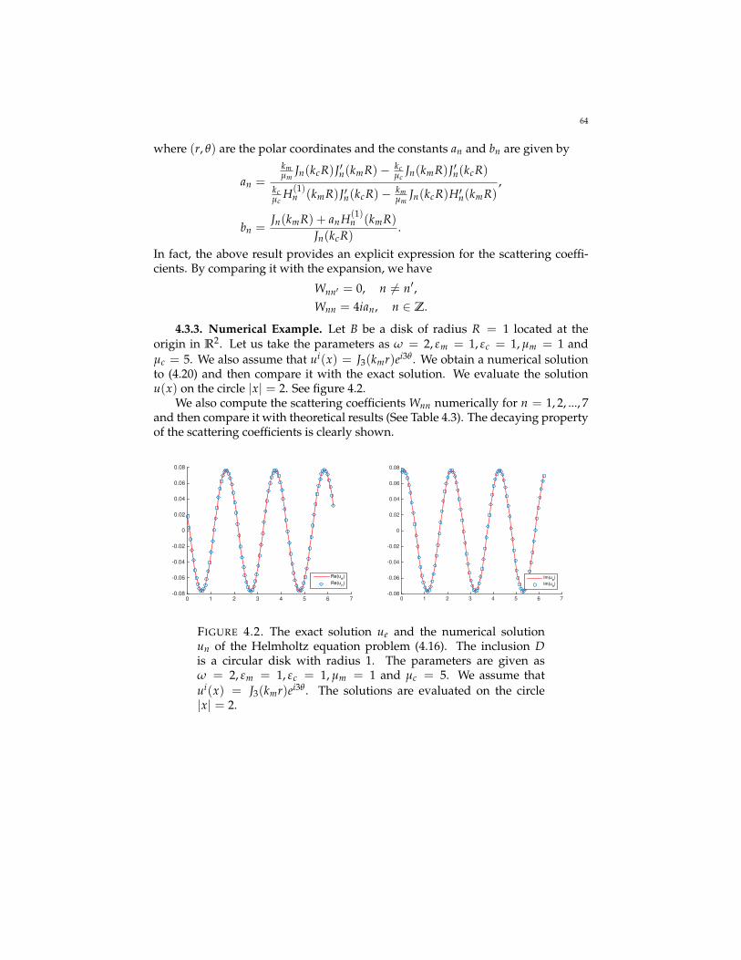
64

where (r, θ) are the polar coordinates and the constants an and bn are given by

an =

kmµm

Jn(kcR)J′n(kmR)− kcµc

Jn(kmR)J′n(kcR)kcµc

H(1)n (kmR)J′n(kcR)− km

µmJn(kcR)H′n(kmR)

,

bn =Jn(kmR) + an H(1)

n (kmR)Jn(kcR)

.

In fact, the above result provides an explicit expression for the scattering coeffi-cients. By comparing it with the expansion, we have

Wnn′ = 0, n 6= n′,Wnn = 4ian, n ∈ Z.

4.3.3. Numerical Example. Let B be a disk of radius R = 1 located at theorigin in R2. Let us take the parameters as ω = 2, εm = 1, εc = 1, µm = 1 andµc = 5. We also assume that ui(x) = J3(kmr)ei3θ . We obtain a numerical solutionto (4.20) and then compare it with the exact solution. We evaluate the solutionu(x) on the circle |x| = 2. See figure 4.2.

We also compute the scattering coefficients Wnn numerically for n = 1, 2, ..., 7and then compare it with theoretical results (See Table 4.3). The decaying propertyof the scattering coefficients is clearly shown.

0 1 2 3 4 5 6 7-0.08

-0.06

-0.04

-0.02

0

0.02

0.04

0.06

0.08

Re(ue)

Re(un)

0 1 2 3 4 5 6 7-0.08

-0.06

-0.04

-0.02

0

0.02

0.04

0.06

0.08

Im(ue)

Im(un)

FIGURE 4.2. The exact solution ue and the numerical solutionun of the Helmholtz equation problem (4.16). The inclusion Dis a circular disk with radius 1. The parameters are given asω = 2, εm = 1, εc = 1, µm = 1 and µc = 5. We assume thatui(x) = J3(kmr)ei3θ . The solutions are evaluated on the circle|x| = 2.

65

n Theoretical Numerical1 1.7866− 1.1036i 1.7866− 1.1011i2 −0.9673− 3.7540i −0.9601− 3.7545i3 −0.6487− 0.1081i −0.6487− 0.1081i4 −0.0462− 0.0005i −0.0462− 0.0005i5 −0.0023− 0.0000i −0.0023− 0.0000i6 −0.0001− 0.0000i −0.0001− 0.0000i7 −0.0000− 0.0000i −0.0000− 0.0000i

TABLE 4.3. Scattering coefficients Wnn for n = 1, 2, ..., 7 when Dis a unit circular disk. The parameters are given as ω = 2, εm =1, εc = 1, µm = 1 and µc = 5.

CHAPTER 5

Direct Imaging and Super-resolution in High ContrastMedia

In this chapter we discuss direct imaging using a MUSIC-type algorithm forinclusion detection, and how super-resolution imaging can be achieved in highcontrast media.

Before discussing the MUSIC-type algorithm for inclusion detection we firsttake a look at Pisarenko’s method for frequency estimation which is essentially aspecial case of the classical MUSIC frequency detection algorithm. Both MUSICand Pisarenko’s method are subspace methods that decompose an autocovariancematrix which characterizes a signal into signal subspace and a noise subspace. InPisarenko’s method the noise subspace is spanned by a single vector whereas inthe MUSIC algorithm d minus p vectors are used to span the noise subspace whered is the number of measurements and p is the number of complex exponentials inthe signal. Both methods proceed along the same lines which as follows:

i) A set of measurements of the data is taken.ii) These measurements are used to construct a matrix that characterizes the

data.iii) The matrix is decomposed into a signal subspace and a noise subspace.iv) A set of test data is generated.v) Elements of the test data set are projected against the noise subspace.

vi) We plot the results and observe large peaks when the parameters usedfor the test data are close to the parameters present in the original data.

5.1. Pisarenko harmonic decomposition

Code: 5.1 Pisarenko Harmonic Decomposition PisarenkoHarmonicDecomposition.m

Let f = f1, f2, . . . , fp be a set of p frequencies and let sj be a complex exponentialgiven by

sj( f j, t) = ei2π f jt, j = 1, . . . , p.Let s( f , t) be a wide sense stationary signal given by summing the p complex ex-ponentials sj. Then the autocovariance function (the inverse Fourier Transform ofthe Power Spectral Density) of the signal s is given by

σss(τ) =p

∑j=1

ei2π f jτ ,

where τ is the lag time. Assume we have measurements for d lag times whered = p + 1. Calculating the autocovariance for τ = 0, . . . , d− 1 lets us construct the

66

http://www.sam.math.ethz.ch/~grsam/HS16/MCMP/Code/Tutorial5/5.1 Pisarenko Harmonic Decomposition.zip

67

autocovariance matrix Css. For example, in the case where d = 3, Css is given by

Css =

σss(0) σss(1) σss(2)σss(1) σss(0) σss(1)σss(2) σss(1) σss(0)

.

The covariance matrix can also be written as

Css =p

∑j=1

sj sHj ,

where sj = (1, ei2π f j , ei4π f j , . . . , ei2π(d−1) f j) represents the jth component of the sig-nal evaluated at the d lag times.

Now suppose the signal also contains noise by defining r( f , t) = s( f , t) + wwhere the noise w has variance σ2. Then the autocovariance matrix is given by

Crr = Css + σ2 Id,

where Id is the identity matrix of dimension d. Crr is a Hermitian matrix with plinearly independent columns so taking an eigendecomposition of Crr gives

Crr = QDQH ,

where D is a diagonal matrix containing the eigenvalues of Crr, ordered as λ1 ≥λ2 ≥ · · · ≥ λd and Q contains orthogonal eigenvectors ψj, j = 1, . . . , d. We have pdegrees of freedom in the data and hence the first p eigenvectors form a basis forwhat is known as the signal subspace. The remaining eigenvector forms a basis forthe noise subspace. Hence the covariance matrix can be written in terms of thesesubspaces as

Crr =p

∑j=1

(λj + σ2)ψjψHj + σ2ψdψH

d .

The fact that the signal subpspace and the noise subspace are othogonal to eachother means that

sj · ψd = 0,and this allows us to determine whether a particular frequency is a component ofthe signal. That is, we consider Ipisa[s( f )] = 1

s( f )·ψdover a range of frequencies f .

If f is close to a frequency in the signal then Ipisa will show a large peak at thislocation.

5.2. Overview of the MUSIC-type algorithm

Code: 5.2 Direct Imaging With MUSIC DemoHelmholtzAnomalyImaging.m

We now focus on imaging small inclusions using a version of the MUSIC algorithmgeared towards inclusion localization. The procedure used in this section can beviewed as a generalization of the much simpler Pisarenko’s method for frequencyestimation.

We probe a medium D using time-harmonic waves emitted from and recordedwith a sensor array. Due to the presence of small inclusions boundary measure-ments of the field will be perturbed slightly from the boundary measurementsgiven by a field in the absence of inclusions. We can use these boundary measure-ment perturbations to define an imaging functional for each combination of emit-ted and received wave. By considering all combinations of emitted and received

http://www.sam.math.ethz.ch/~grsam/HS16/MCMP/Code/Tutorial5/5.2 Direct Imaging With MUSIC.zip

68

waves for a finite set of sources and receivers we can define a set of imaging func-tionals. These imaging functionals are used to construct a multi-static responsemarix (MSR) A which is analogous to the covariance matrix Css in Pisarkeno’smethod.

Once we have calculated the MSR matrix which characterizes the data wemust generate a set of test data over a range of inclusion locations. We projectthis test data against the noise subspace of the MSR matrix and this leads to largepeaks at position which correspond to the locations of the inclusions.

It is should be noted that the distance from the inclusions to the boundary, andthe distance from the inclusions to each other should be much greater than thewavelength. If this is not the case the effective rank of the singular value decom-position of the MSR matrix will be reduced and we will not be able to differentiatethe inclusions.

5.2.1. Multistatic Response Matrix: Statistical Structure. In multistatic waveimaging, waves are emitted by a set of sources and they are recorded by a set ofsensors in order to probe an unknown medium. The responses between each pairof source and receiver are collected and assembled in the form of the multi-staticresponse (MSR) matrix. The indices of the MSR matrix are the index of the sourceand the index of the receiver. When the data are corrupted by additive noise, westudy the structure of the MSR matrix using random matrix theory.

In the standard acquisition scheme, the response matrix is measured during asequence of Ns experiments. In the mth experiment, m = 1, . . . , Ns, the mth sourcegenerates the incident field and the Nr receivers record the scattered wave whichmeans that they measure

Ameasnm = A0

nm + Wnm, n = 1, . . . , Nr, m = 1, . . . , Ns ,

which gives the matrix

(5.1) Ameas = A0 + W ,

where A0 is the unperturbed response matrix and Wnm are independent complexGaussian random variables with mean zero and variance σ2

noise (which means thatthe real and imaginary parts are independent real Gaussian random variables withmean zero and variance σ2

noise/2).Throughout this section, we only consider the two-dimensional full-view case,

where the sensor arrays englobe the reflectors or the inclusions to be imaged.

5.2.2. Point Reflectors and SVD of Multistatic Response Matrices. Supposethat ε0 = µ0 = 1. Consider the Helmholtz equation:

(5.2) ∆zΦω(z, x) + ω2(

1 +r

∑j=1

Vj(z))

Φω(z, x) = δx(z) in R2

for x ∈ R2, with the Sommerfeld radiation condition imposed on Φω. Here r isthe number of localized reflectors, x is the location of the source, and

(5.3) Vj(z) := ηjχ(Dj)(z− zj) ,

where, for j = 1, . . . , r, Dj is a compactly supported domain with volume |Dj|,χ(Dj) is the characteristic function of Dj, zj is the center of the jth inclusion, and

69

ηj := ε j − 1 is the dielectric contrast (also called the strength of the point reflectorat zj).

Suppose that we have a transmitter array of Ns sources located at x1, . . . , xNsand a receiver array of Nr elements located at y1, . . . , yNr. The Nr × Ns responsematrix A describes the transmit-receive process performed at these arrays. Thefield received by the nth receiving element yn when the wave is emitted from xmis Φω(yn, xm). If we remove the incident field then we obtain the (n, m)-th entryof the unperturbed response matrix A0:

(5.4) A0nm = −Φω(yn, xm) + Γω(yn, xm) .

The incident field is Γω(y, xm).Finally, taking into account measurement noise, the measured response matrix

Ameas is

(5.5) Ameas = A0 +1√Ns

W ,

where the matrix W represents the additive measurement noise, which is a randommatrix with independent and identically distributed complex entries with Gaus-sian statistics, mean zero and variance σ2

noise. This particular scaling for the noiselevel is the right one to get non-trivial asymptotic regimes in the limit Ns → ∞.Furthermore, it is the regime that emerges from the use of the Hadamard acquisi-tion scheme for the response matrix.

In the Born approximation, where the volume |Dj| of Dj, j = 1, . . . , r, goesto zero, the measured field has approximately the following form. We include aproof for the readers’ sake.

THEOREM 5.1. We have

(5.6) Φω(yn, xm) ≈ Γω(yn, xm)−r

∑j=1

ρjΓω(yn, zj)Γω(zj, xm)

for n = 1, . . . , Nr, m = 1, . . . , Ns, where ρj is the coefficient of reflection defined by

(5.7) ρj = ω2ηj|Dj| .

PROOF. Suppose for simplicity that the number of reflectors is 1 (r = 1). Let usconsider the full fundamental solution Φω(z, x) and the background fundamentalsolution Γω(z, y), namely,

∆zΦω(z, x) + ω2Φω(z, x) = −ω2V(z)Φω(z, x) + δx(z)

∆zΓω(z, y) + ω2Γω(z, y) = δy(z) ,

with the radiation condition. We multiply the first equation by Γω(x, y) and sub-tract the second equation multiplied by Φω(x, z):

∇z ·[Γω(z, y)∇zΦω(z, x)−Φω(z, y)∇zΓω(z, x)

]= −ω2V(z)Φω(z, x)Γω(z, y) + Γω(z, y)δx(z)−Φω(z, x)δy(z)

= −ω2V(z)Φω(z, x)Γω(z, y) + Γω(x, y)δx(z)−Φω(y, x)δy(z)reciprocity

= −ω2V(z)Φω(x, z)Γω(z, y) + Γω(x, y)δx(z)−Φω(x, y)δy(z) .

70

We integrate over BR (with R large enough so that it encloses the support of V)and send R to infinity to obtain thanks to the Sommerfeld radiation condition that

0 = −ω2ˆ

R2Φω(x, z)V(z)Γω(z, y)dz + Γω(x, y)−Φω(x, y) .

We therefore obtain the Lippmann-Schwinger equation, which is exact:

Φω(x, y) = Γω(x, y)−ω2ˆ

R2Φω(x, z)V(z)Γω(z, y)dz .

This equation is used as a basis for expanding the fundamental solution Φω whenthe reflectivity V is small. If Φω in the right-hand side is replaced by the back-ground fundamental solution Γω, then we obtain:

(5.8) Φω(x, y) ≈ Γω(x, y)−ω2ˆ

Γω(x, z)V(z)Γω(z, y)dz ,

which is the (first-order) Born approximation. When the volume |D1| is small, theintegral in (5.8) can be replaced by −ω2η1|D1|Γω(x, z1)Γω(z1, y), which gives thedesired result.

We introduce the normalized vector of fundamental solutions from the re-ceiver array to the point z:

(5.9) w(z) :=1(

∑Nrl=1 |Γω(z, yl)|2

) 12

(Γω(z, yn)

)n=1,...,Nr

,

and the normalized vector of fundamental solutions from the transmitter array tothe point z, known as the illumination vector,

(5.10) v(z) :=1(

∑Nsl=1 |Γω(z, xl)|2

) 12

(Γω(z, xm)

)m=1,...,Ns

.

Using (5.6) we can then write the unperturbed response matrix approximatelyin the form

(5.11) A0 =r

∑j=1

σjw(zj)v(zj)∗ ,

with

(5.12) σj := ρj

( Nr

∑n=1|Γω(zj, yn)|2

) 12( Ns

∑m=1|Γω(zj, xm)|2

) 12

.

Here ∗ denotes the conjugate transpose.We assume that the arrays of transmitters and receivers are equi-distributed

on a disk englobing the point reflectors. Moreover, the point reflectors are at a dis-tance from the arrays of transmitter and receivers much larger than the wavelength2π/ω. Provided that the positions zj of the reflectors are far from one another orwell-separated (i.e., farther than the wavelength 2π/ω), the vectors w(zj), j =1, . . . , r, are approximately orthogonal to one another, as well as are the vectorsv(zj), j = 1, . . . , r. In fact, from the Helmholtz-Kirchhoff identity, we have

(5.13)1

Nr∑n

Γω(zj, yn)Γω(zi, yn) ≈1ω

J0(ω|zi − zj|)

71

as Nr → +∞, where J0 is the Bessel function of the first kind and of order zero.Moreover, J0(ω|zi − zj|) ≈ 0 when |zj − zi| is much larger than the wavelength.The matrix A0 then has rank r and its nonzero singular values are σj, j = 1, . . . , r,with the associated left and right singular vectors w(zj) and v(zj).

5.2.3. Helmholtz Equation. Suppose that an electromagnetic medium occu-pies a bounded domain Ω in Rd, with a connected C2-boundary ∂Ω. Suppose thatΩ contains a small inclusion of the form D = δB + z, where z ∈ Ω and B is aC2-bounded domain in Rd containing the origin.

Let µ0 and ε0 denote the permeability and the permittivity of the backgroundmedium Ω, and assume that µ0 and ε0 are positive constants. Let µ? and ε? denotethe permeability and the permittivity of the inclusion D, which are also assumedto be positive constants. Introduce the piecewise constant magnetic permeability

µδ(x) =

µ0 , x ∈ Ω \ D ,µ? , x ∈ D .

The piecewise constant electric permittivity, εδ(x), is defined analogously.Let the electric field u denote the solution to the Helmholtz equation

(5.14) ∇ · ( 1µδ∇u) + ω2εδu = 0 in Ω ,

with the boundary condition u = f ∈W212(∂Ω), where ω > 0 is a given frequency.

Problem (5.14) can be written as

(∆ + ω2ε0µ0)u = 0 in Ω \ D ,

(∆ + ω2ε?µ?)u = 0 in D ,1

µ?

∂u∂ν

∣∣∣∣−− 1

µ0

∂u∂ν

∣∣∣∣+

= 0 on ∂D ,

u∣∣− − u

∣∣+= 0 on ∂D ,

u = f on ∂Ω .

Assuming that

ω2ε0µ0 is not an eigenvalue for the operator − ∆ in L2(Ω)

with homogeneous Dirichlet boundary conditions,(5.15)

we can prove existence and uniqueness of a solution to (5.14) at least for δ smallenough.

THEOREM 5.2 (Boundary Perturbations). Suppose that (5.15) holds. Let u be thesolution of (5.14) and let the function U be the background solution as before. For anyx ∈ ∂Ω,

∂u∂ν

(x) =∂U∂ν

(x) + δd(∇U(z) ·M(λ, B)

∂∇zGk0(x, z)∂νx

+ k20(

ε?ε0− 1)|B|U(z)

∂Gk0(x, z)∂νx

)+ O(δd+1) ,(5.16)

72

where M(λ, B) is the polarization tensor defined in (4.4) with λ given by

(5.17) λ :=(µ0/µ?) + 1

2((µ0/µ?)− 1).

Here Gk0 is the Dirichlet Green.

5.2.4. Formal Derivations. From the Lippman-Schwinger integral represent-ation formula

u(x) = U(x) + (µ0

µ?− 1)

ˆD∇u(y) · ∇yGk0(x, y) dy

+ k20(

ε?ε0− 1)

ˆD

u(y)Gk0(x, y) dy, x ∈ Ω ,

it follows that for any x ∈ ∂Ω,

∂u∂ν

(x) =∂U∂ν

(x) + (µ0

µ?− 1)

ˆD∇u(y) · ∂∇yGk0(x, y)

∂νxdy

+ k20(

ε?ε0− 1)

ˆD

u(y)∂Gk0(x, y)

∂νxdy .

Using a Taylor expansion of Gk0(x, y) for y ∈ D, we readily see that for any x ∈ ∂Ω,

(5.18)

∂u∂ν

(x) ≈ ∂U∂ν

(x) + (µ0

µ?− 1)

∂∇zGk0(x, z)∂νx

· (ˆ

D∇u(y) dy)

+ k20(

ε?ε0− 1)

∂Gk0(x, z)∂νx

(

ˆD

u(y) dy) .

By taking an asymptotic expansion one can easily check that u(y) ≈ U(z), fory ∈ D, and ˆ

D∇u(y) dy ≈ δd

( ˆB∇v(ξ) dξ

)· ∇U(z) ,

where v is the solution to:

(5.19)

∆v = 0 in Rd \ B ,∆v = 0 in B ,v|− − v|+ = 0 on ∂B ,

k∂v∂ν|− −

∂v∂ν|+ = 0 on ∂B ,

v(ξ)− ξ → 0 as |ξ| → +∞ .

with k = µ0/µ?. Next, we computeˆB∇v(ξ) dξ =

ˆB(I +∇SB(λI −K∗B)−1[ν](ξ)) dξ

= |B|I +ˆ

∂B(−1

2I +K∗B)(λI −K∗B)−1[ν](ξ)ξT dσ(ξ)

=1

k− 1

ˆ∂B(λI −K∗B)−1[ν](ξ) ξT dσ(ξ) ,

where |B| is the volume of B. Inserting these two approximations into (5.18) leadsto (5.16).

73

Before concluding this section, we make a remark. Consider the Helmholtzequation with the Neumann data g in the presence of the inclusion D:

(5.20)

∇ · 1

µδ∇u + ω2εδu = 0 in Ω ,

∂u∂ν

= g on ∂Ω .

Let the background solution U satisfy

(5.21)

∆U + k20U = 0 in Ω ,

∂U∂ν

= g on ∂Ω .

The following asymptotic expansion of the solution of the Neumann problemholds. For any x ∈ ∂Ω, we have

u(x) = U(x) + δd(∇U(z)M(λ, B)∇zNk0(x, z)

+ k20(

ε?ε0− 1)|B|U(z)Nk0(x, z)

)+ O(δd+1) ,(5.22)

where Nk0 is the Neumann function defined by

(5.23)

∆x Nk0(x, z) + k0

2Nk0(x, z) = −δz in Ω ,∂Nk0

∂νx

∣∣∣∂Ω

= 0 for z ∈ Ω .

The following useful relation between the Neumann function and the funda-mental solution Γk0 holds:

(5.24) (−12

I +Kk0Ω )[Nk0(·, z)](x) = Γk0(x, z), x ∈ ∂Ω, z ∈ Ω .

5.2.5. Direct imaging algorithms for the Helmholtz equation at a fixed fre-quency. In this section, we design direct imaging functionals for small inclusionsat a fixed frequency ω. Consider the Helmholtz equation (5.20) with the Neu-mann data g in the presence of the inclusion D and let the background solution Ube defined by (5.21).

Let w be a smooth function such that (∆ + k20)w = 0 in Ω. The weighted

boundary measurements Iw[U, ω] defined by

(5.25) Iw[U, ω] :=ˆ

∂Ω(u−U)(x)

∂w∂ν

(x) dσ(x)

satisfies

(5.26)Iw[U, ω] = −δd

(∇U(z) ·M(λ, B)∇w(z) + k2

0(ε?ε0− 1)|B|U(z)w(z)

)+ o(δd) ,

with λ given by (5.17).We apply the asymptotic formulas (5.16) and (5.26) for the purpose of identi-

fying the location and certain properties of the inclusions.

74

Consider P well-separated inclusions Dp = zp + δBp, p = 1, . . . , P. The mag-netic permeability and electric permittivity of Dp are denoted by µp and εp, re-spectively. Suppose that all the domains Bp are disks. In this case, we have

Iw[U, ω] ≈ −P

∑p=1|Dp|

(2

µp − µ0

µ0 + µp∇U(z) · ∇w(z) + k2

0(εp

ε0− 1)U(z)w(z)

).

5.2.6. MUSIC-type algorithm. Let (θ1, . . . , θn) be n unit vectors in Rd. Forθ ∈ θ1, . . . , θn, we assume that we are in possession of the boundary data uwhen the domain Ω is illuminated with the plane wave U(x) = eik0θ·x. Taking theharmonic function w(x) = e−ik0θ′ ·x for θ′ ∈ θ1, . . . , θn and using (4.9) shows thatthe weighted boundary measurement is approximately equal to

Iw[U, ω] ≈ −P

∑p=1|Dp|k2

0

(2

µ0 − µp

µ0 + µpθ · θ′ + εp

ε0− 1)

eik0(θ−θ′)·zp .

Define the response matrix A = (All′)nl,l′=1 ∈ Cn×n by

(5.27) All′ := Iwl′ [Ul , ω] ,

where Ul(x) = eik0θl ·x, wl(x) = e−ik0θl ·x, l = 1, . . . , n. It is approximately given by

(5.28) All′ ≈ −P

∑p=1|Dp|k2

0

(2

µ0 − µp

µ0 + µpθl · θl′ +

εp

ε0− 1)

eik0(θl−θl′ )·zp ,

for l, l′ = 1, . . . , n. Introduce the n-dimensional vector fields g(j)(zS), for zS ∈ Ωand j = 1, . . . , d + 1, by

(5.29) g(j)(zS) =1√n(ej · θ1eik0θ1·zS

, . . . , ej · θneik0θn ·zS)T , j = 1, . . . , d ,

and

(5.30) g(d+1)(zS) =1√n(eik0θ1·zS

, . . . , eik0θn ·zS)T ,

where e1, . . . , ed is an orthonormal basis of Rd. Let g(zS) be the n × d matrixwhose columns are g(1)(zS), . . . , g(d)(zS). Then (5.28) can be written as

A ≈ −nP

∑p=1|Dp|k2

0

(2

µ0 − µp

µ0 + µpg(zp)g(zp)

T+ (

εp

ε0− 1)g(d+1)(zp)g(d+1)(zp)

T).

Let Pnoise = I − P, where P is the orthogonal projection onto the range of A asbefore. The MUSIC-type imaging functional is defined by

(5.31) IMU(zS, ω) :=( d+1

∑j=1‖Pnoise[g(j)](zS)‖2

)−1/2.

This functional has large peaks only at the locations of the inclusions.

75

µ ε

MUSIC reconstruction Backprojection Kirchhoff migration

FIGURE 5.1. Top: The magnetic inclusion with coefficient µ andthe electrical inclusion with coefficient ε in the domain Ω. Bottom:Reconstructed fields using MUSIC, backprojection, and Kirchhoffmigration.

5.2.7. Backpropagation-type algorithms. Let (θ1, . . . , θn) be n unit vectors inRd. A backpropagation-type imaging functional at a single frequency ω is givenby

(5.32) IBP(zS, ω) :=1n

n

∑l=1

e−2ik0θl ·zSIwl [Ul , ω] ,

where Ul(x) = wl(x) = eik0θl ·x, l = 1, . . . , n. Suppose that (θ1, . . . , θn) are equidistantpoints on the unit sphere Sd−1. For sufficiently large n, we have

(5.33)1n

n

∑l=1

eik0θl ·x ≈ 4(π

k0)d−2 =m

Γk0(x, 0)

=

sinc(k0|x|) for d = 3 ,J0(k0|x|) for d = 2 ,

where sinc(s) = sin(s)/s is the sinc function and J0 is the Bessel function of thefirst kind and of order zero.

Therefore, it follows that

IBP(zS, ω) ≈ −P

∑p=1|Dp|k2

0

(2

µp − µ0

µ0 + µp+(

εp

ε0− 1)

)×

sinc(2k0|zS − zp|) for d = 3,J0(2k0|zS − zp|) for d = 2 .

76

These formulas show that the resolution of the imaging functional is the standarddiffraction limit. It is of the order of half the wavelength λ = 2π/k0.

Note that IBP uses only the diagonal terms of the response matrix A, definedby (5.27). Using the whole matrix, we arrive at the Kirchhoff migration functional:

(5.34) IKM(zS, ω) =d+1

∑j=1

g(j)(zS) · Ag(j)(zS) ,

where g(j) are defined by (5.29) and (5.30).

5.3. Super-resolution in high contrast media

It is well-known that the resolution in the homogeneous space for far-fieldimaging system is limited by half the operating wave-length, which is a direct con-sequence of Abbe’s diffraction limit. In order to differentiate point sources whichare located less than half the wavelength apart, super-resolution techniques haveto be used. While many techniques exist in practice, here we are only interested inone using resonant media.

The basic idea is the following: suppose that we have sources that are denselylocated in a homogeneous space of size the wavelength of the wave the sourcescan emit, and we want to differentiate them by making measurements in the far-field. While this is impossible in the homogeneous space, it is possible if the me-dium around these sources is changed so that the point spread function, whichis the imaginary part of the Green function in the new medium, displays a muchsharper peak than the homogeneous one and thus can resolve sub-wavelength de-tails. The key issue in such an approach is to design the surrounding mediumso that the corresponding Green function has the tailored property. In this section,we develop the mathematical theory for realizing this approach by using high con-trast media. We show that in high contrast media the super-resolution is due to thepropagating sub-wavelength resonant modes excited in the media and is limitedby the finest structure in these modes.

We also explain how to compute Green’s function numerically and presentan example to show a sharp peak of imaginary part of Green’s function can beachieved using high contrast media.

5.3.1. Green’s Function for a high-contrast resonator. Throughout this sec-tion, we put the wavenumber ω to be the unit and suppress its presence in whatfollows. We assume that the wave speed in the free space is one. The free-spacewavelength is given by 2π. We consider the following Helmholtz equation with adelta source term:

∆xG(x, x0) + G(x, x0) + τn(x)χ(D)(x)G(x, x0) = δ(x− x0) in Rd,(5.35)

where χ(D) is the characteristic function of D, which has size of order of the freespace wavelength, n(x) is a positive function of order one in the space of C1(D)and τ 1 is the contrast. We denote by G0(x, x0) the free-space Green’s functionΓ1(x− x0).

Write G = v + G0, we can show that

(5.36) ∆v + v = −τn(x)χ(D)(v + G0).

77

Thus,

v(x, x0) = −τ

ˆD

n(y)G0(x, y)(

v(y, x0) + G0(y, x0)

)dy.

Define

(5.37) KD[ f ](x) = −ˆ

Dn(x)G0(x, y) f (y) dy.

Then, v = v(x) = v(x, x0) satisfies the following integral equation:

(5.38) (I − τKD)[v] = τKD[G(·, x0)],

and hence,

v(x) = (1τ− KD)

−1KD[G(·, x0)].

In what follows, we present properties of the integral operator KD.

LEMMA 5.3. The operator KD is compact from L2(D) to L2(D). In fact, KD isbounded from L2(D) to H2(D). Moreover, KD is a Hilbert-Schmidt operator.

LEMMA 5.4. Let σ(KD) be the spectrum of KD defined by (5.37). We have(i) σ(KD) = 0, λ1, λ2, ..., λn, ...., where |λ1| ≥ |λ2| ≥ |λ3| ≥ ... and λn → 0;

(ii) 0 = σ(KD)\σp(KD) with σp(KD) being the point spectrum of KD.

PROOF. We need only to prove the second assertion. Assume that KD[u] =´D G0(x, y)n(y)u(y) dy = 0. We have 0 = (4+ 1)KD[u] = nu, which shows that

u = 0. The assertion is then proved.

LEMMA 5.5. Let KD be defined by (5.37). Then, λ ∈ σ(KD) if and only if there is anontrivial solution in H2

loc(Rd) to the following problem:

(∆ + 1)u(x) = 1λ n(x)u(x) in D,(5.39)

(∆ + 1)u = 0 in Rd\D,(5.40)u satisfies the Sommerfeld radiation condition.(5.41)

PROOF. Assume that KD[u] = λu. We define u(x) =´

D G0(x, y)n(y)u(y) dy,where x ∈ Rd. Then u satisfies the required equations.

Notice that the resonant modes have sub-wavelength structures in D for |λ| <1.

LEMMA 5.6. Let Hj denote the generalized eigenspace of the operator KD for theeigenvalue λj. The following decomposition holds:

L2(D) =∞⋃

j=1

Hj.

PROOF. By the same argument as the one in the proof of Lemma 5.4, we canshow that Ker K∗D = 0. As a result, we have

KD(

L2(D))=(Ker K∗D

)⊥= L2(D).

The lemma is proved.

78

LEMMA 5.7. There exists a basis uj,l,k, 1 ≤ l ≤ mj, 1 ≤ k ≤ nj,l forHj such that

KD(uj,1,1, ..., uj,mj ,nj,mj) = (uj,1,1, ..., uj,mj ,nj,mj

)

Jj,1. . .

Jj,mj

,

where Jj,l is the canonical Jordan matrix of size nj,l in the form

Jj,l =

λj 1

. . . . . .λj 1

λj

.

PROOF. This follows from the Jordan theory applied to the linear operatorKD|Hj : Hj → Hj on the finite dimensional spaceHj.

We denote Γ = (j, l, k) ∈ N×N×N; 1 ≤ l ≤ mj, 1 ≤ k ≤ nj,l the set ofindices for the basis functions. We introduce a partial order on N×N×N. Letγ = (j, k, l) ∈ Γ, γ′ = (j′, l′, k′) ∈ Γ, we say that γ′ γ if one of the followingconditions are satisfied:

(i) j > j′;(ii) j = j′, l > l′;

(iii) j = j′, l = l′, k ≥ k′.By Gram-Schmidt orthonormalization process, the following result is obvious.

LEMMA 5.8. There exists orthonormal basis eγ : γ ∈ Γ for L2(D) such that

eγ = ∑γ′γ

aγ,γ′uγ′ ,

where aγ,γ′ are constants and aγ,γ 6= 0.

We can regard A = aγ,γ′γ,γ′∈Γ as a matrix. It is clear that A is upper-triangular and has non-zero diagonal elements. Its inverse is denoted by B =bγ,γ′γ,γ′∈Γ which is also upper-triangular and has non-zero diagonal elements.We have

uγ = ∑γ′γ

bγ,γ′ eγ′ .

LEMMA 5.9. The functions eγ(x)eγ′(y) form a normal basis for the Hilbert spaceL2(D× D). Moreover, the following completeness relation holds:

δ(x− y) = ∑γ

eγ(x)eγ(y).

By standard elliptic theory, we have G(x, x0) ∈ L2(D × D) for fixed τ. Thuswe have

(5.42) G(x, x0) = ∑γ,γ′

αγ,γ′ eγ(x)eγ′(x0),

for some constants αγ,γ′ satisfying

∑γ,γ′|αγ,γ′ |2 = ‖G(x, x0)‖2

L2(D×D) < ∞.

79

To analyze the Green function G, we need to find the constants αγ,γ′ . For doingso, we first note that

G0(x, x0) =1

n(x0)KD[δ(· − x0)].

Thus,

G(x, x0) = G0(x, x0) + (1τ− KD)

−1K2D[δ(· − x0)]

= G0(x, x0) +1

n(x0)∑γ

eγ(x0)(1τ− KD)

−1K2D[eγ].

We next compute ( 1τ − KD)

−1K2D[eγ]. For ease of notation, we define uj,l,k = 0

for k ≤ 0. We have

KD[uj,l,k] = λjuj,l,k + uj,l,k−1 for all j, l, k,

K2D[uj,l,k] = λ2

j uj,l,k + 2λjuj,l,k−1 + uj,l,k−2 for all j, l, k.

On the other hand, for z /∈ σ(KD), we have

(z− KD)−1[uj,l,k] =

1z− λj

uj,l,k +1

(z− λj)2 uj,l,k−1 + ... +1

(z− λj)k uj,l,1,

and therefore, it follows that

(z− KD)−1K2

D[uj,l,k] =λ2

j

z− λjuj,l,k +

λ2j

(z− λj)2 uj,l,k−1 · · ·+λ2

j

(z− λj)k uj,l,1

+2λj

z− λjuj,l,k−1 +

2λj

(z− λj)2 uj,l,k−2 · · ·+2λj

(z− λj)k−1 uj,l,1

+1

z− λjuj,l,k−2 +

1(z− λj)2 uj,l,k−3 · · ·+

1(z− λj)k−2 uj,l,1

=λ2

j

z− λjuj,l,k +

( λ2j

(z− λj)2 +2λj

z− λj

)uj,l,k−1

+( λ2

j

(z− λj)3 +2λj

z− λj+

1z− λj

)uj,l,k−2

+... +( λ2

j

(z− λj)k +2λj

(z− λj)k−1 +1

(z− λj)k−2

)uj,l,1

= ∑γ′

dγ,γ′uγ′ ,

where we have introduced the matrix D = dγ,γ′γ,γ′∈Γ, which is upper-triangularand has block-structure.

With these calculations, by taking z = 1/τ, we arrive at the following result.

THEOREM 5.10. The following expansion holds for the Green function

(5.43) G(x, x0) = G0(x, x0) + ∑γ∈Γ

∑γ′′′∈Γ

αγ,γ′′′ eγ(x0)eγ′′′(x),

80

whereα

γ,γ′′′ =1

n(x0)∑

γ′γ∑

γ′′γ′

aγ,γ′dγ′ ,γ′′ bγ′′ ,γ′′′ .

Moreover, for τ−1 belonging to a compact subset of R \(R ∩ σ(KD)

), we have the

following uniform bound:∑γ,γ′|αγ,γ′ |2 < ∞.

Alternatively, if we start from the identity,

δ(x− x0) = ∑γ′′

eγ′′(x)eγ′′(x0)

= ∑γ′′

∑γ′γ′′

∑γ′′′γ′′

aγ′′ ,γ′ aγ′′ ,γ′′′uγ′(x)uγ′′′(x0),

then we can obtain an equivalent expansion for the Green function in terms of thebasis of resonant modes.

THEOREM 5.11. The following expansion holds for the Green function:

(5.44) G(x, x0) = G0(x, x0) + ∑γ′′∈Γ

∑γ′′′γ

′′∑

γγ′′

βγ′′ ,γ,γ′′′ uγ(x)u

γ′′′ (x0),

where

(5.45) βγ′′ ,γ,γ′′′ =

1n(x0)

∑γ′γ

′′a

γ′′ ,γ′′′ aγ

′′ ,γ′dγ′ ,γ.

Here, the infinite summation can be interpreted as follows:(5.46)

limγ0→∞ ∑

γ′′≤γ0

∑γ′γ′′

∑γ′′′γ′′


γ′′′ (x0) = G(x, x0)−G0(x, x0) in L2(D×D).

In order to have some idea of the expansions of the Green function G(x, y), wecompare them to the expansion of the Green function in the homogeneous space,i.e., G0(x, y). For this purpose, we introduce the matrix H = hγ,γ′γ,γ′∈Γ, whichis defined by

KD[uγ] = ∑γ′

hγ,γ′uγ′ .

In fact, we have

hj,l,k,j′ ,l′ ,k′ = λjδj,j′δl,l′δk,k′ + δj,j′δl,l′δk−1,k′ ,

where δ denotes the Kronecker symbol.

LEMMA 5.12. (i) In the normal basis eγγ∈Γ, the following expansion holdsfor the Green function G0(x, x0):

(5.47) G0(x, x0) = ∑γ∈Γ

∑γ′′′∈Γ

αγ,γ′′′ eγ(x0)eγ′′′(x),

whereα

γ,γ′′′ =1

n(x0)∑

γ′γ∑

γ′′γ′

aγ,γ′hγ′ ,γ′′ bγ′′ ,γ′′′ .

81

Moreover, we have the following uniform bound:

∑γ,γ′|αγ,γ′ |2 < C < ∞.

(ii) In the basis of resonant modes uγγ∈Γ, the following expansion holds for theGreen function G0(x, x0):

(5.48) G0(x, x0) = ∑γ′′∈Γ

∑γ′′′γ

′′∑

γγ′′


γ′′′ (x0),

where

(5.49) βγ′′ ,γ,γ′′′ =

1n(x0)

∑γ′γ

′′a

γ′′ ,γ′′′ aγ

′′ ,γ′hγ′ ,γ.

Here, the infinite summation can be interpreted as follows:

limγ0→∞ ∑

γ′′≤γ0

∑γ′′′γ

′′∑

γγ′′


γ′′′ (x0) = G0(x, x0) in L2(D× D).

By comparing the coefficients αγ,γ′ (or βγ,γ′ ) and αγ,γ′ (or βγ,γ′ ), we can seethat the imaginary part of G(x, y) may have a sharper peak than G0(x, y) due tothe excited high frequency resonant modes.


Code: 5.3 Super-resolution in High Contrast Media DemoGreenHighContrast.m

In this section we explain how to compute the Green’s function numerically. Wealso present a numerical example in which a high contrast medium is representedas a disk.

5.4.1. Solving an integral equation for the Green’s function. The Green’sfunction G is the solution to the following problem:

(5.50)

∇ ·1µ∇G(·, x0) + ω2εG(·, x0) =

1µc

δx0 in Rd,

G(·, x0) satisfies the Sommerfeld radiation condition.

It can be shown that the above problem is equivalent to the following system ofequations:

(5.51)

(∆ + k2c)G(·, x0) = δx0 in D,

(∆ + k2m)G(·, x0) = 0 in Rd \ D,

G(·, x0)|+ = G(·, x0)|− on ∂D,1

µm

∂G(·, x0)

∂ν

∣∣∣+=

1µc

∂G(·, x0)

∂ν

∣∣∣−

on ∂D,

G(·, x0) satisfies the Sommerfeld radiation condition.

Note that here the wave number kc plays the role of the high contrast parameteranalogously to τ in the previous theoretical analysis.

Let Gkc0 be the free space Green’s function with a wave number kc. Since Gkc

0satisfies

(5.52) (∆ + k2c)G

kc0 (·, x0) = δx0 , in Rd,

http://www.sam.math.ethz.ch/~grsam/HS16/MCMP/Code/Tutorial5/5.3 Super-resolution in High Contrast Media.zip

82

we see that v := G − Gkc0 satisfies ∆v + k2

c v = 0 in D. So we can represent theGreen’s function G using the single layer potential as follows:

(5.53) G(x, x0) =

Gkc

0 (x, x0) + SkcD [ϕ](x), x ∈ D,

SkmD [ψ](x), x ∈ Rd \ D,

Next we determine the density functions ϕ and ψ. From the transmissionconditions on ∂D and the jump relations for the single layer potentials, we get(5.54)Skc

D [ϕ]− SkmD [ψ] = −Gkc

0 (·, x0)

1µc

(−12

I + (KkcD )∗)[ϕ]

∣∣∣∣−− 1

µm(

12

I + (KkmD )∗)[ψ]

∣∣∣∣+

= − 1µc

∂Gkc0 (·, x0)

∂ν

on ∂D.

The above integral equation has the same form as that of (4.20). We have alreadydiscussed how to solve that equation numerically in the previous chapter.

5.4.2. Explicit expression of Green’s function for a disk. For the special caseof the domain B, we can obtain an explicit solution to the transmission problem.Let B be a disk of radius R located at the origin in R2. Then it can be shown thatthe explicit solution is given by

(5.55) G(r, θ) =

−i4

H(1)0 (kcr) + aJ0(kcr), |r| ≤ R,

bH(1)0 (kmr), |r| > R,

where (r, θ) are the polar coordinates and the constants a and b are given by

a = − i4

kmµm

H(1)0 (kcR)(H(1)

0 )′(kmR)− kcµc

H(1)0 (kmR)(H(1)

0 )′(kcR)kcµc

H(1)0 (kmR)J′0(kcR)− km

µmJ0(kcR)(H(1)

0 )′(kmR),

b = − i4

kcµc

H(1)0 (kcR)J′0(kcR)− kc

µc(H(1)

0 )′(kcR)J0(kcR)kcµc

H(1)0 (kmR)J′0(kcR)− km

µmJ0(kcR)(H(1)

0 )′(kmR).

5.4.3. Resonant wave number kc for a disk. It is also worth emphasizing thatwe can derive resonant values for kc. From the expressions for a and b, we canimmediately see that the n-th resonant value kc,n is n-th zero of

(5.56)kc

µcH(1)

0 (kmR)J′0(kcR)− km

µmJ0(kcR)(H(1)

0 )′(kmR) = 0.

So the resonant values for kc can be computed using Muller’s method. When wesolve the above equation, we need to be careful because µc depends on kc viaµc = k2

c /(ω2εc).

5.4.4. Numerical example. Let D be a disk of radius R = 2 centered at theorigin O in R2. We fix ω = 1, εc = εm = 1 and µm = 1. Then µc is determined byµc = k2

c .First, let us compute how the resonant values for kc are distributed. In order to

do this, we plot the LHS of (5.56) as a function of kc. The plot is shown in Figure 5.2and it shows that there are many local maximum points which converge to zero astheir corresponding wave number kc increases. It reflects the fact that the reson-ant values kc,n (or the corresponding eigenvalues of the operator KD) are complex

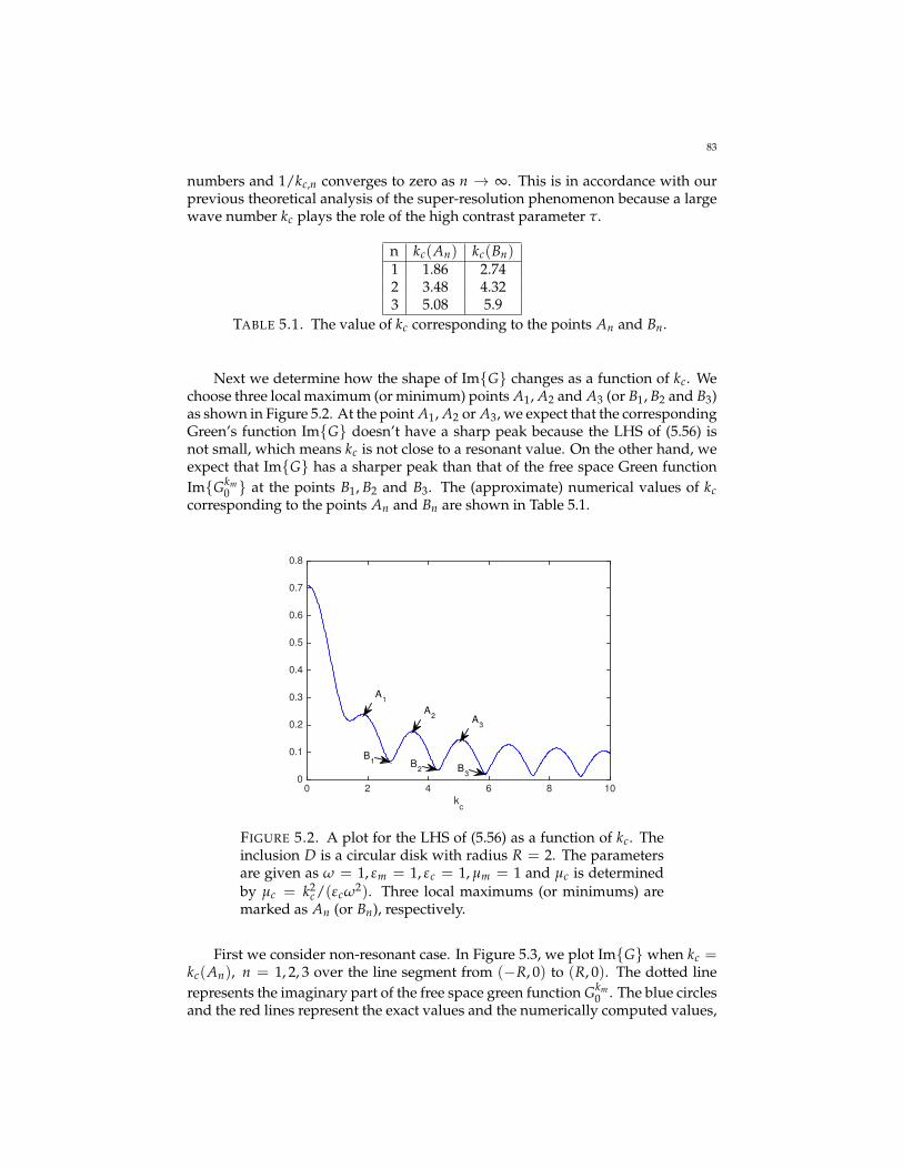
83

numbers and 1/kc,n converges to zero as n → ∞. This is in accordance with ourprevious theoretical analysis of the super-resolution phenomenon because a largewave number kc plays the role of the high contrast parameter τ.

n kc(An) kc(Bn)1 1.86 2.742 3.48 4.323 5.08 5.9

TABLE 5.1. The value of kc corresponding to the points An and Bn.

Next we determine how the shape of ImG changes as a function of kc. Wechoose three local maximum (or minimum) points A1, A2 and A3 (or B1, B2 and B3)as shown in Figure 5.2. At the point A1, A2 or A3, we expect that the correspondingGreen’s function ImG doesn’t have a sharp peak because the LHS of (5.56) isnot small, which means kc is not close to a resonant value. On the other hand, weexpect that ImG has a sharper peak than that of the free space Green functionImGkm

0 at the points B1, B2 and B3. The (approximate) numerical values of kccorresponding to the points An and Bn are shown in Table 5.1.

kc

0 2 4 6 8 100

0.1

0.2

0.3

0.4

0.5

0.6

0.7

0.8

A3

A2

A1

B3

B2

B1

FIGURE 5.2. A plot for the LHS of (5.56) as a function of kc. Theinclusion D is a circular disk with radius R = 2. The parametersare given as ω = 1, εm = 1, εc = 1, µm = 1 and µc is determinedby µc = k2

c /(εcω2). Three local maximums (or minimums) aremarked as An (or Bn), respectively.

First we consider non-resonant case. In Figure 5.3, we plot ImG when kc =kc(An), n = 1, 2, 3 over the line segment from (−R, 0) to (R, 0). The dotted linerepresents the imaginary part of the free space green function Gkm

0 . The blue circlesand the red lines represent the exact values and the numerically computed values,

84

respectively. We note that in this case the peak is not sharper than that of the freespace Green’s function.

Next, we consider the resonant case. In Figure 5.4, we plot ImG when kc =kc(Bn), n = 1, 2, 3 over the line segment from (−R, 0) to (R, 0). In contrast to theprevious case, in the case of a resonant kc the peak is sharper than that of the freespace Green’s function. Also the subwavelength structure of the resonant mode isclearly shown.

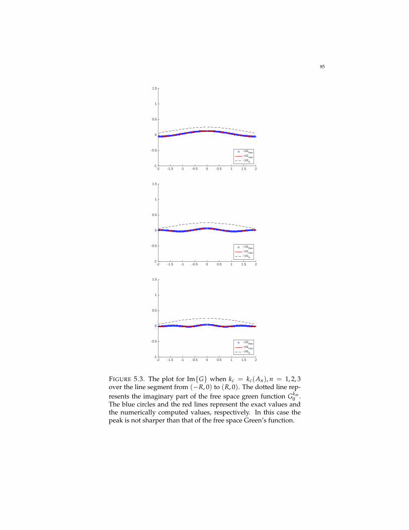
85

-2 -1.5 -1 -0.5 0 0.5 1 1.5 2-1

-0.5

0

0.5

1

1.5

-=Gtheo

-=Gnum

-=G0

-2 -1.5 -1 -0.5 0 0.5 1 1.5 2-1

-0.5

0

0.5

1

1.5

-=Gtheo

-=Gnum

-=G0

-2 -1.5 -1 -0.5 0 0.5 1 1.5 2-1

-0.5

0

0.5

1

1.5

-=Gtheo

-=Gnum

-=G0

FIGURE 5.3. The plot for ImG when kc = kc(An), n = 1, 2, 3over the line segment from (−R, 0) to (R, 0). The dotted line rep-resents the imaginary part of the free space green function Gkm

0 .The blue circles and the red lines represent the exact values andthe numerically computed values, respectively. In this case thepeak is not sharper than that of the free space Green’s function.

86

-2 -1.5 -1 -0.5 0 0.5 1 1.5 2-1

-0.5

0

0.5

1

1.5

-=Gtheo

-=Gnum

-=G0

-2 -1.5 -1 -0.5 0 0.5 1 1.5 2-1

-0.5

0

0.5

1

1.5

-=Gtheo

-=Gnum

-=G0

-2 -1.5 -1 -0.5 0 0.5 1 1.5 2-1

-0.5

0

0.5

1

1.5

-=Gtheo

-=Gnum

-=G0

FIGURE 5.4. The plot for ImG when kc = kc(Bn), n = 1, 2, 3over the line segment from (−R, 0) to (R, 0). The dotted linerepresents the imaginary part of the free space green functionGkm

0 . The blue circles and the red lines represent the exact valuesand the numerically computed values, respectively. In this casethe peak is sharper than that of the free space Green’s function.Also the subwavelength structure of the resonant mode is clearlyshown.

CHAPTER 6

Maxwell’s Equations and Scattering Coefficients

In this chapter, we consider the full Maxwell’s equations along with the in-tegral representation of their solution. We also introduce the concept of scatteringcoefficients in the context of Maxwell’s equations. We demonstrate how the scat-tering coefficients for a multi-layer spherical shell can be computed. A numericalexample is also provided.

6.1. Maxwell’s equations

6.1.1. Time harmonic Maxwell’s equations. Here we introduce Maxwell’sequations which describe general electromagnetic fields. Consider the time-dependentMaxwell’s equations ∇× E = −µ ∂

∂tH,∇×H = ε ∂

∂tE ,where µ is the magnetic permeability and ε is the electric permittivity.

In the time-harmonic regime, one looks for electromagnetic fields of the form H(x, t) = H(x)e−iωt,E(x, t) = E(x)e−iωt,

where ω is the frequency. The pair (E, H) is a solution to the harmonic Maxwellequations

(6.1) ∇× E = iωµH,∇× H = −iωεE.

One says that (E, H) is radiating if it satisfies the Silver-Müller radiation condition:

lim|x|→∞

|x|(√µH × x−√

εE) = 0,

where x = x/|x|. In the sequel, one sets the wave number k = ω√

εµ.

6.1.2. Layer potentials. Assume that D is bounded, simply connected, and ofclass C1,η for η > 0 and let

HsT(∂D) =

ϕ ∈

(Hs(∂D)

)3, ν · ϕ = 0

.

We introduce the surface gradient, surface divergence and Laplace-Beltramioperator and denote them by ∇∂D, ∇∂D· and ∆∂D, respectively. We define thevectorial and scalar surface curl by ~curl∂D ϕ = −ν×∇∂D ϕ for ϕ ∈ H

12 (∂D) and

87

88

curl∂D ϕ = −∇∂D · (ν× ϕ) for ϕ ∈ H−12

T (∂D), respectively. We recall that

∇∂D · ∇∂D = ∆∂D,

curl∂D ~curl∂D = −∆∂D,

∇∂D · ~curl∂D = 0,curl∂D∇∂D = 0.

We introduce the following functional space:

H−12

T (div, ∂D) =

ϕ ∈ H−

12

T (∂D),∇∂D · ϕ ∈ H−12 (∂D)

.

Define the following boundary integral operators:

~SkD[ϕ] : H−

12

T (∂D) −→ H12T (∂D) or H1

loc(R3)3

ϕ 7−→ ~SkD[ϕ](x) =

ˆ∂D

Γk(x− y)ϕ(y)dσ(y);

MkD[ϕ] : H−

12

T (div, ∂D) −→ H−12

T (div, ∂D)

ϕ 7−→ MkD[ϕ](x) =

ˆ∂D

ν(x)×∇x × Γk(x− y)ϕ(y)dσ(y);

LkD[ϕ] : H−

12

T (div, ∂D) −→ H−12

T (div, ∂D)

ϕ 7−→ LkD[ϕ](x) = ν(x)×

(k2~Sk

D[ϕ](x) +∇SkD[∇∂D · ϕ](x)

).

The operator ~SkD satisfies the following jump formmula.(

ν×∇× ~SkD[ϕ]

)∣∣∣±∂D

= (∓12

I +MkD)[ϕ].

Furthermore it holds that(ν×∇×∇× ~Sk

D[ϕ])∣∣∣

∂D= Lk

D[ϕ].

6.1.3. Layer potential formulation for electromagnetic scattering. We con-sider the scattering problem of a time-harmonic electromagnetic wave incidenton D. The homogeneous medium is characterized by electric permittivity εm andmagnetic permeability µm, while D is characterized by electric permittivity εc andmagnetic permeability µc, both of which depend on the frequency. Define

km = ω√

εmµm, kc = ω√

εcµc,

andεD = εmχ(R3 \ D) + εcχ(D), µD = εmχ(R3 \ D) + εcχ(D).

For a given incident plane wave (Ei, Hi) that is a solution to the Maxwell equa-tions in free space, that is,

(6.2) ∇× Ei =

√−1ωµm Hi in R3,

∇× Hi = −√−1ωεmEi in R3,

89

the scattering problem can be modeled by the following system of equations:

(6.3)

∇× E =

√−1ωµD H in R3 \ ∂D,

∇× H = −√−1ωεDE in R3 \ ∂D,

ν× E∣∣+− ν× E

∣∣− = ν× H

∣∣+− ν× H

∣∣− = 0 on ∂D,

subject to the Silver-Müller radiation condition:

lim|x|→∞

|x|(√

µm(H − Hi)(x)× x|x| −

√εm(E− Ei)(x)

)= 0(6.4)

uniformly in x/|x|.Using the boundary integral operators ~Sk

D,MkD and Lk

D, the solution to (6.3)can be represented as(6.5)

E(x) =

Ei(x) + µm∇× ~Skm

D [ψ](x) +∇×∇× ~SkmD [φ](x), x ∈ R3 \ D,

µc∇× ~SkcD [ψ](x) +∇×∇× ~Skc

D [φ](x), x ∈ D,

and

(6.6) H(x) = −√−1

ωµD(∇× E)(x) x ∈ R3 \ ∂D,

where the pair (ϕ, ψ) ∈(

H−12

T (div, ∂D))2 satisfies

(6.7)µc + µm

2I + µcMkc

D − µmMkmD Lkc

D −LkmD

LkcD −Lkm

D

(k2

c2µc

+k2

m2µm

)I +

k2c

µcMkc

D −k2

mµmMkm

D

[ ψφ

]

=

[ν× Ei√−1ων× Hi

] ∣∣∣∣∣∂D

.

It can be shown that that the system of equations (6.7) on TH(div, ∂D) ×TH(div, ∂D) has a unique solution and there exists there a positive constant C =C(ε, µ, ω) such that(6.8)‖ψ‖TH(div,∂D) + ‖φ‖TH(div,∂D) ≤ C

(‖Ei × ν‖TH(div,∂D) + ‖Hi × ν‖TH(div,∂D)

).

6.2. Scattering coefficients

6.2.1. Multipole solutions to the Maxwell equations. For a wave numberk > 0, l′ = −l, . . . , l and l = 1, 2, . . . , the function

(6.9) vll′(k; x) = h(1)l (k|x|)Yl′l (x)

satisfies the Helmholtz equation ∆v + k2v = 0 in R3 \ 0 and the Sommerfeldradiation condition:

lim|x|→∞

|x|(∂vll′

∂|x| (k; x)−√−1kvll′(k; x)) = 0.

Here, Yl′l is the spherical harmonic defined on the unit sphere S, x = x/|x|, and

h(1)l is the spherical Hankel function of the first kind and order l which satisfies the

90

Sommerfeld radiation condition in three dimensions. Similarly, we define vll′(x)by

(6.10) vll′(k; x) = jl(k|x|)Yl′l (x),

where jl is the spherical Bessel function of the first kind. The function vll′ satisfiesthe Helmholtz equation in all R3.

In a similar manner, one can form solutions to the Maxwell system with thevector version of spherical harmonics. Define the vector spherical harmonics as

(6.11) Ull′ =1√

l(l + 1)∇SYl′

l (x) and Vll′ = x×Ull′ ,

for l′ = −l, . . . , l and l = 1, 2, . . . . Here, x ∈ S and∇S denotes the surface gradienton the unit sphere S. The vector spherical harmonics defined in (6.11) form acomplete orthogonal basis for L2

T(S), where L2T(S) = u ∈ (L2(S))3 | ν · u = 0

and ν is the outward unit normal to S.By multiplying the vector spherical harmonics with the Hankel function, one

can construct so-called multipole solutions to the Maxwell system. To keep theanalysis simple, one separates the solutions into transverse electric, (E · x) = 0,and transverse magnetic, (H · x) = 0. Define the exterior transverse electric mul-tipoles to the Maxwell equations in free space as

(6.12)

ETE

ll′ (k; x) = −√

l(l + 1)h(1)l (k|x|)Vll′(x),

HTEll′ (k; x) = −

√−1

ωµ∇×

(−√

l(l + 1)h(1)l (k|x|)Vll′(x))

,

and the exterior transverse magnetic multipoles as

(6.13)

ETMll′ (k; x) =

√−1

ωε∇×

(−√

l(l + 1)h(1)l (k|x|)Vll′(x))

,

HTMll′ (k; x) = −

√l(l + 1)h(1)l (k|x|)Vll′(x).

The exterior electric and magnetic multipole satisfy the radiation condition. Inthe same manner, one defines the interior multipoles (ETE

ll′ , HTEll′ ) and (ETM

ll′ , HTMll′ )

with h(1)l replaced by jl , i.e.,

(6.14)

ETE

ll′ (k; x) = −√

l(l + 1)j(1)l (k|x|)Vll′(x),

HTEll′ (k; x) = −

√−1

ωµ∇× ETE

ll′ (k; x),

and

(6.15)

HTM

ll′ (k; x) = −√

l(l + 1)j(1)l (k|x|)Vll′(x),

ETMll′ (k; x) =

√−1

ωε∇× HTM

ll′ (k; x).

91

Note that one has

∇× ETEll′ (k; x) =

√l(l + 1)|x| Hl(k|x|)Ull′(x) +

l(l + 1)|x| h(1)l (k|x|)Yl′

l (x)x,(6.16)

∇× ETEll′ (k; x) =

√l(l + 1)|x| Jl(k|x|)Ull′(x) +

l(l + 1)|x| j(1)l (k|x|)Yl′

l (x)x,(6.17)

whereHl(t) = h(1)l (t) + t(

h(1)l

)′(t) and Jl(t) = jl(t) + tj′l(t).

The solutions to the Maxwell system can be represented as separated vari-able sums of the multipole solutions. Using multipole solutions together with theHelmholtz solutions in (6.9) and (6.10), it is also possible to expand the funda-mental solution Γk to the Helmholtz operator.

Let p be a fixed vector in R3. For |x| > |y|, the following addition formulaholds:

Γk(x− y)p =−∞

∑l=1

√−1k

l(l + 1)ε

µ

l

∑l′=−l

ETMll′ (k; x)ETM

ll′ (k; y) · p

+∞

∑l=1

√−1k

l(l + 1)

l

∑l′=−l

ETEll′ (k; x)ETE

ll′ (k; y) · p

−√−1k

∞

∑l=1

l

∑l′=−l

∇vll′(k; x)∇vll′(k; y) · p,(6.18)

with vll′ and vll′ being defined by (6.9) and (6.10).Plane wave solutions to the Maxwell equations have expansions using multi-

pole solutions as well. The incoming wave

Ei(x) =√−1k(q× p)× qe

√−1kq·x,

where q ∈ S is the direction of propagation and the vector p ∈ R3 is the directionof polarization, is expressed as(6.19)

Ei(x) =√−1k

∞

∑l=1

4π(√−1)l√

l(l + 1)

l

∑l′=−l

[(Vll′(q) · c

)ETE

ll′ (x)− 1√−1ωµ

(Ull′(q) · c

)ETM

ll′ (x)]

,

where c = (q× p)× q.

6.2.2. Scattering coefficients. This subsection introduces the notion of scat-tering coefficients associated with the Maxwell equations. It extends the notionsand results established in the previous section for the Helmholtz equation.

From (6.18) (with km in the place of k) and (6.5) it follows that, for sufficientlylarge |x|,

(6.20) (E− Ei)(x) =∞

∑l=1

√−1km

l(l + 1)

l

∑l′=−l

(αll′E

TEll′ (km; x) + βll′E

TMll′ (km; x)

),

where

αll′ = −√−1ωεmµm

ˆ∂D

ETMll′ (km; y) · ϕ(y) + k2

m

ˆ∂D

ETEll′ (km; y) · ψ(y),

βll′ = −√−1ωεmµm

ˆ∂D

ETEll′ (km; y) · ϕ(y)−ω2ε2

m

ˆ∂D

ETMll′ (km; y) · ψ(y).

92

Let (ϕTEpp′ , ψTE

pp′) be the solution to (6.7) when

Ei = ETEpp′(km; y) and Hi = HTE

pp′(km; y),

and (ϕTMpp′ , ψTM

pp′ ) when

Ei = ETMpp′ (km; y) and Hi = HTM

pp′ (km; y).

DEFINITION 6.1 (Scattering Coefficients). The scattering coefficients(WTE,TE

ll′ ,pp′ , WTE,TMll′ ,pp′ , WTM,TE

ll′ ,pp′ , WTM,TMll′ ,pp′

)associated with the permittivity and the permeability distributions ε, µ and thefrequency ω (or kc, km, D) are defined to be

WTE,TEll′ ,pp′ = −

√−1ωεmµm

ˆ∂D

ETMll′ (km; y) · ϕTE

pp′(y) dσ(y) + k2m

ˆ∂D

ETEll′ (km; y) · ψTE

pp′(y) dσ(y),

WTE,TMll′ ,pp′ = −

√−1ωεmµm

ˆ∂D

ETMll′ (km; y) · ϕTM

pp′ (y) dσ(y) + k2m

ˆ∂D

ETEll′ (km; y) · ψTM

pp′ (y) dσ(y),

WTM,TEll′ ,pp′ = −

√−1ωεmµm

ˆ∂D

ETEll′ (km; y) · ϕTE

pp′(y) dσ(y)−ω2ε2m

ˆ∂D

ETMll′ (km; y) · ψTE

pp′(y) dσ(y),

WTM,TMll′ ,pp′ = −

√−1ωεmµm

ˆ∂D

ETEll′ (km; y) · ϕTM

pp′ (y) dσ(y)−ω2ε2m

ˆ∂D

ETMll′ (km; y) · TM

pp′ (y) dσ(y).

As can be seen, the scattering coefficients appear naturally in the expansion ofthe scattering amplitude. One first obtains the following estimates for the decayof the scattering coefficients.

LEMMA 6.2. There exists a constant C depending on (ε, µ, ω) such that

(6.21)∣∣∣WTE,TE

ll′ ,pp′ [ε, µ, ω]∣∣∣ ≤ Cl+p

ll pp

for all l, l′, p, p′ ∈N. The same estimates hold for WTE,TMll′ ,pp′ , WTM,TE

ll′ ,pp′ , and WTM,TMll′ ,pp′ .

PROOF. Let (ϕ, ψ) be the solution to (6.7) with Ei(y) = ETEpp′(km; y) and Hi =

−√−1

ωµm∇× Ei. Recall that the spherical Bessel function jp behaves as

jp(t) =tp

1 · 3 · · · (2p + 1)

(1 + O

(1p

))as p→ ∞,

uniformly on compact subsets of R. Using Stirling’s formula

p! =√

2πp(p/e)p(1 + o(1)),

one has

(6.22) jp(t) = O(

Cptp

pp

)as p→ ∞,

uniformly on compact subsets of R with a constant C independent of p. Thus onehas ∥∥Ei∥∥

TH(div,∂D)+∥∥Hi∥∥

TH(div,∂D)≤ C′p

pp

93

for some constant C′. It then follows from (6.8) that∥∥ϕ∥∥

L2(∂D)+∥∥ψ∥∥

L2(∂D)≤ Cp

pp

for another constant C. So one gets (6.21) from the definition of the scatteringcoefficients.

Now suppose that the incoming wave is of the form

(6.23) Ei(x) =∞

∑p=1

p

∑p′=−p

(app′ E

TEpp′(km; x) + bpp′ E

TMpp′ (km; x)

)for some constants app′ and bpp′ . Then the solution (ϕ, ψ) to (6.7) is given by

ϕ =∞

∑p=1

p

∑p′=−p

(app′ϕ

TEpp′ + bpp′ϕ

TMpp′

),

ψ =∞

∑p=1

p

∑p′=−p

(app′ψ

TEpp′ + bpp′ψ

TMpp′

).

By (6.20) and Definition 6.1, the solution E to (6.3) can be represented as(6.24)

(E− Ei)(x) =∞

∑l=1

√−1km

l(l + 1)

l

∑l′=−l

(αll′E

TEll′ (km; x) + βll′E

TMll′ (km; x)

), |x| → ∞,

where

(6.25)

αll′ =

∞

∑p=1

p

∑p′=−p

(app′W

TE,TEll′ ,pp′ + bpp′W

TE,TMll′ ,pp′

),

βll′ =∞

∑p=1

p

∑p′=−p

(app′W

TM,TEll′ ,pp′ + bpp′W

TM,TMll′ ,pp′

).

6.3. Multi-layer structure and its scattering coefficients

Code: 6.1 Scattering Coefficients for Maxwell’s Equations DemoSCoeffMaxwell.m

Here we consider a multi-layered structure and explain how to compute itsscattering coefficients. A numerical example is also presented. The multi-layeredstructure is defined as follows: For positive numbers r1, . . . , rL+1 with 2 = r1 >r2 > · · · rL+1 = 1, let

Aj := x : rj+1 ≤ |x| < rj, j = 1, . . . , L,

A0 := R3 \ B2(0), AL+1(= D) := x : |x| < 1,where B2(0) denotes the central ball of radius 2 and

Γj = |x| = rj, j = 1, . . . , L + 1.

Let (µj, εj) be the pair of permeability and permittivity parameters of Aj for j =1, . . . , L + 1. Set µ0 = 1 and ε0 = 1. Then define the permeability and permittivity

http://www.sam.math.ethz.ch/~grsam/HS16/MCMP/Code/Tutorial6/6.1 Scattering Coefficients for Maxwell's Equations.zip

94

distributions of the layered structure to be

(6.26) µ =L+1

∑j=0

µjχ(Aj) and ε =L+1

∑j=0

εjχ(Aj).

A0

…A1

ALAL+1

PEC

rL rL-1

r1

ϵ1, μ1 ϵ0, μ0

ϵL, μL

…

…

FIGURE 6.1. a multi-layered structure

The scattering coefficients(

WTE,TE(n,m)(p,q), WTE,TM

(n,m)(p,q), WTM,TE(n,m)(p,q), WTM,TM

(n,m)(p,q)

)are

defined as before, namely, if Ei given as in (6.23), the scattered field E− Ei can beexpanded as (6.24) and (6.25). The transmission condition on each interface Γj isgiven by

(6.27) [x× E] = [x× H] = 0.

Assume that the core AL+1 is perfectly conducting (PEC), that is,

(6.28) E× ν = 0 on ΓL+1 = ∂AL+1.

Thanks to the symmetry of the layered (radial) structure, the scattering coeffi-cients are much simpler than the general case. In fact, if the incident field is givenby Ei = ETE

n,m, then the solution E to (6.1) takes the form

(6.29) E(x) = ajETEn,m(x) + ajETE

n,m(x), x ∈ Aj, j = 0, . . . , L,

with a0 = 1. From (6.16) and (6.17), the interface condition (6.27) amounts to jn(k jrj) h(1)n (k jrj)1µjJn(k jrj)

1µjHn(k jrj)

[ajaj

]

=

jn(k j−1rj) h(1)n (k j−1rj)1

µj−1Jn(k j−1rj)

1µj−1Hn(k j−1rj)

[aj−1aj−1

], j = 1, . . . , L,(6.30)

95

where Hn(t) = h(1)n (t) + t(

h(1)n

)′(t) and Jn(t) = jn(t) + tj′n(t), and the PEC

boundary condition on ΓL+1 is

(6.31)

[jn(kL) h(1)n (kL)

0 0

] [aLaL

]=

[00

].

Since the matrices appearing in (6.30) are invertible, one can see that there exist ajand aj, j = 0, 1, . . . L satisfying (6.30) and (6.31). Similarly, one can see that if theincident field is given by Ei = ETM

n,m (x), then the solution E takes the form

(6.32) E(x) = bjETMn,m (x) + bjETM

n,m (x), x ∈ Aj, j = 0, 1, ..., L

for some constants bj and bj (b0 = 1). One can see now from (6.29) and (6.32) thatthe scattering coefficients satisfy

WTE,TM(n,m)(p,q) = WTM,TE

(n,m)(p,q) = 0 for all (m, n) and (p, q),

WTE,TE(n,m)(p,q) = WTM,TM

(n,m)(p,q) = 0 if (m, n) 6= (p, q),

and, since (6.29) and (6.32) hold independently of m, one has

WTE,TE(n,0)(n,0) = WTE,TE

(n,m)(n,m),

WTM,TM(n,0)(n,0) = WTM,TM

(n,m)(n,m)for − n ≤ m ≤ n.

Moreover, if one writes

WTEn := WTE

(n,0)(n,0) and WTMn := WTM

(n,0)(n,0),

then one has

(6.33) WTEn = − in(n + 1)

k0a0 and WTE

n = − in(n + 1)k0

b0.

Suppose now that ETEn,0 is the incident field and the solution E is given by

E(x) = ajETEn,0(x) + ajETE

n,0(x), x ∈ Aj, j = 0, . . . , L,

with a0 = 1, where the coefficients aj’s and aj’s are determined by (6.30) and (6.31).From (6.30) it follows that

[ajaj

]=

jn(k jrj) h(1)n (k jrj)1µjJn(k jrj)

1µjHn(k jrj)

−1 jn(k j−1rj) h(1)n (k j−1rj)

1µj−1Jn(k j−1rj)


[aj−1aj−1

],

for j = 1, . . . , L. Substituting these relations into (6.31) yields

(6.34)[

00

]= PTE

n [ε, µ, ω]

[a0a0

],

96

where

PTEn [ε, µ, ω] :=

[pTE

n,1 pTEn,2

0 0

]= (−iω)L

(L

∏j=1

µ32j ε

12j rj

)[jn(kL) h(1)n (kL)

0 0

]

×L

∏j=1

1µjHn(k jrj) −h(1)n (k jrj)

− 1µjJn(k jrj) jn(k jrj)

jn(k j−1rj) h(1)n (k j−1rj)

1µj−1Jn(k j−1rj)


.

(6.35)

Then (6.34) yields

(6.36) WTEn = − in(n + 1)

k0a0 = − in(n + 1)

k0

pTEn,1

pTEn,2

.

Similarly, for WTMn , one looks for another solution E of the form

E(x) = bjETMn,0 (x) + bjETM

n,0 (x), x ∈ Aj, j = 0, ..., L,

with b0 = 1. The transmission conditions become 1εjJn(k jrj)

1εjHn(k jrj)

jn(k jrj) h(1)n (k jrj)

[bjbj

]

=

1εj−1Jn(k j−1rj)

1εj−1Hn(k j−1rj)


[bj−1bj−1

], j = 1, . . . , N + 1,(6.37)

and the PEC boundary condition on the inner most layer is

(6.38)[Jn(kL) Hn(kL)

0 0

] [bLbL

]=

[00

].

From (6.37) and (6.38), one obtains

(6.39)[

00

]= PTM

n [ε, µ, ω]

[b0b0

],

where

PTMn [ε, µ, ω] :=

[pTM

n,1 pTMn,2

0 0

]= (iω)L

(L

∏j=1

µ12j ε

32j rj

)[Jn(kL) Hn(kL)0 0

]

×L

∏j=1

h(1)n (k jrj) − 1εjHn(k jrj)

−jn(k jrj)1εjJn(k jrj)

1

εj−1Jn(k j−1rj)

1εj−1Hn(k j−1rj)


.

(6.40)

From the definition of WTMn and (6.39),

(6.41) WTEn = − in(n + 1)

k0

b0

b0= − in(n + 1)

k0

pTMn,1

pTMn,2

.

97

It is worth emphasizing that pTEn,2 6= 0 and pTM

n,2 6= 0. In fact, if pTEn,2 = 0, then

(6.34) can be fulfilled with a0 = 0 and a0 = 1. This means that there exists (µ, ε)on R3 \ D such that the following problem has a solution:

∇× E = iωµH in R3 \ D,∇× H = −iωεE in R3 \ D,(x× E)

∣∣+= 0 on ∂D,

E(x) = ETEn,0(x) for |x| > 2.

Applying the following Green’s theorem on Ω = x∣∣ 1 < |x| < R,ˆ

Ω

(E · ∆F + curlE · curlF + divE divF

)dx

=

ˆ∂Ω

(ν× E · curlF + ν · E divF

)dσ(x)

with F = ETEn,0(x) and the PEC boundary condition on |x| = 1, it follows thatˆ

|x|=R(ν× E) · Hdσ(x) = ik0

ˆΩ(|H|2 − |E|2)dx.

In particular, the left-hand side is real-valued. Hence,ˆ|x|=R

|H × ν− E|2dσ(x) =ˆ|x|=R

(|H × ν|2 + |E|2 − 2<((ν× E) · H

)dσ(x)

=

ˆ|x|=R

(|H × ν|2 + |E|2

)dσ(x).

From the radiation condition, the left-hand side goes to zero as R → ∞, whichcontradicts the behavior of the Hankel functions. One can show that pTM

n,2 6= 0 in asimilar way.

6.3.1. Numerical example. Here we demonstrate how the scattering coeffi-cients WTE

n and WTMn can be computed numerically and then present an example.

For simplicity, we consider only WTEn . Recall that

(6.42) WTEn = − in(n + 1)

k0a0,

and the constant a0 is determined by (6.30) and (6.31). From (6.30), we obtain

(6.43)[

a0/aLa0/aL

]= (M−1

1 N1)(M−12 N2) . . . (M−1

L NL)

[aL/aL

1

],

where

Mj =

jn(k jrj) h(1)n (k jrj)1µjJn(k jrj)

1µjHn(k jrj)

, Nj =

jn(k j−1rj) h(1)n (k j−1rj)1

µj−1Jn(k j−1rj)


.

From (6.31), we immediately see that

aLaL

= −h(1)n (kLrL+1)

jn(kLrL+1).

Therefore, we can compute a0/aL and a0/aL. But, since a0 = 1, we can also com-pute a0 and then WTE

n .

98

Now we present a numerical example. We set the parameters for the structureas follows: the number of layers L is L = 3, the radii of layers are r1 = 2, r2 =5/3, r3 = 4/3, r4 = 1, and the material parameters are (ε0, µ0) = (1, 1), (ε0, µ0) =(0.5, 0.5), (ε0, µ0) = (2, 2), (ε0, µ0) = (0.5, 0.5). The numerical result for WTE

n andWTM

n for n = 1, 2, ..., 7 is shown in Table 6.1. The decaying behavior of WTEn and

WTMn is clearly shown.

n WTEn WTM

n1 −0.9991 + 0.9572i −0.7473 + 1.6644i2 −0.7527 + 0.0960i −0.7650 + 0.0992i3 −0.1642 + 0.0022i −0.1643 + 0.0023i4 −0.0191 + 0.0000i −0.0191 + 0.0000i5 −0.0013 + 0.0000i −0.0013 + 0.0000i6 −0.0001 + 0.0000i −0.0001 + 0.0000i7 −0.0000 + 0.0000i −0.0000 + 0.0000i

TABLE 6.1. Scattering coefficients for a multi-layer spherical shell

CHAPTER 7

Diffraction Gratings

In this chapter we discuss periodic structures with tiny spatial features knownas diffraction gratings in which light propagation is governed by diffraction. Thefull Maxwell’s equations are used to model the energy distribution in systems in-volving such gratings. However, if the fields are composed of transverse time-harmonic electromagnetic waves we can reduce the Maxwell equations to twoscalar Helmholtz equations. We analyze two classes of gratings:

• linear grating (one-dimensional gratings),• crossed gratings (biperiodic or two-dimensional gratings).

We show how the diffraction grating problem can be formulated in terms of aboundary integral representation. We conclude with a demonstration of how theboundary integral representation can be used to numerically determine the electricfield in the case of a linear grating.

7.0.1. Time-Harmonic Maxwell’s Equations. The electromagnetic wave propaga-tion is governed by Maxwell’s equations. Throughout, we shall restrict our atten-tion to time-harmonic electromagnetic fields with time dependence (e−

√−1ωt), i.e.,

E(x, t) = E(x)e−√−1ωt ,(7.1)

H(x, t) = H(x)e−√−1ωt(7.2)

for some operating frequency ω > 0 with E and H being respectively the electricand magnetic field.

The time-harmonic Maxwell equations take the following form:

∇× E =√−1ωµH,(7.3)

∇× H = −√−1ωεE,(7.4)

where µ is the magnetic permeability and ε is the electric permittivity. Note thatfrom (7.3) and (7.4), it follows that

∇ · (εE) = 0,(7.5)∇ · (µH) = 0.(7.6)

The fields are further assumed to be nonmagnetic and µ = µ0 (usually themagnetic permeability of vacuum). Then (7.6) becomes

∇ · H = 0.

It follows from (7.3-7.4) that the following jump conditions hold:• the tangential components of E and H must be continuous crossing an

interface,

99

100

Incident plane wave

Region I

Region II

FIGURE 7.1. Grating geometry.

• the normal components of εE and H must be continuous crossing an in-terface.

In a homogeneous and isotropic medium, ε does not depend on x. By takingthe curl of (7.3) we obtain that

−∆E +∇(∇ · E) =√−1ωµ0∇× H.

Using (7.4), we have−∆E +∇(∇ · E) = ω2εµ0E

or the Helmholtz equation

(7.7) ∆E + k2E = 0

with k = ω√

εµ0.Similarly, H satisfies

∆H + k2H = 0.Note that in a dielectric medium k2 is real and positive. The wavelength λ is givenby λ = (2π)/k.

7.0.2. Grating Geometry and Fundamental Polarizations. Throughout, a grat-ing is always assumed to be infinitely wide.

Figure 7.1 shows the grating geometry. We denote the period, height, andincident angle by Λ, h, and θ, respectively.

An alternative way to specify the periodicity is by means of ε.For a 1-D grating (linear grating):

ε(x1 + nΛ, x2) = ε(x1, x2), n ∈ Z.

In the case of a crossed grating with period Λ = (Λ1, Λ2) we have

ε(x1 + n1Λ1, x2 + n2Λ2, x3) = ε(x1, x2, x3), ∀ n1, n2 ∈ Z.

We assume that above the interface ε is real and positive. However, below theinterface the parameter ε can be real which corresponds to a dielectric medium;complex corresponding to an absorbing or lossy medium; or perfectly conducting.

In the next three sections we shall discuss two separate cases: The perfectlyconducting grating and the dielectric grating.

101

Suppose that a grating is illuminated under the incidence θ by a plane waveof unit amplitude propagating in Region I (Figure 7.1). The incident vector Ki liesin the (x1, x2) plane

Ki = k1(sin θ,− cos θ, 0).The electromagnetic fields are assumed to be independent of x3. We consider thefollowing two fundamental cases of polarization: TE (transverse electric) and TM(transverse magnetic).

In TE polarization, the electric field is parallel to the grooves or points in thex3 direction, i.e.,

E = u(x1, x2)e3

where u is a scalar function and (e1, e2, e3) is an orthonormal basis of R3.In TM polarization, the magnetic field is parallel to the grooves

H = u(x1, x2)e3.

As we shall see, the resulting Maxwell equations in these two polarizationscan be quite different.

7.0.3. Perfectly Conducting Gratings. In this section, the grating is assumedto be perfectly conducting. In order to treat the two fundamental polarizationssimultaneously, we denote u = E3(x1, x2) in TE polarization; = H3(x1, x2) in TMpolarization, where the subscript 3 stands for the third component. Assume thatthe grating is expressed by x2 = f (x1). Then u = 0 in Region II (x2 < f (x1)). InRegion I, the field u satisfies

(7.8) ∆u + k2u = 0 if x2 > f (x1).

We next derive the boundary condition of u on x2 = f (x1). Using the jump condi-tions and that E is zero in Region II, we have

(7.9) ν× E = 0 on x2 = f (x1),

where ν is the outward normal to Region II.In TE polarization, E = (0, 0, u), hence (7.9) implies that

(7.10) u(x1, f (x1)) = 0,

i.e., a homogeneous Dirichlet boundary condition.In TM polarization, H = (0, 0, u). We obtain by using Maxwell’s equations

and the condition (7.9) that

(7.11)∂u∂ν

∣∣∣∣x2= f (x1)

= 0,

which is a homogeneous Neumann boundary condition.Define the scattered field as the difference between the total field u and the

incident field ui = e√−1(αx1−βx2)

(7.12) us = u− ui.

Here,

(7.13)

α = k1 sin θ,β = k1 cos θ.

102

Since the incident field ui satisfies the Helmholtz equation everywhere, we caneasily show that

(7.14) ∆us + k21us = 0 for x2 > f (x1).

From (7.10) and (7.11), us satisfies either one of the following boundary conditions:TE polarization:

(7.15) us = −ui on x2 = f (x1).

TM polarization:

(7.16)∂us

∂ν= −∂ui

∂νon x2 = f (x1).

Next, since the problem is posed in an unbounded domain, a radiation condition isneeded. We assumed that us is bounded when x2 goes to infinity and consisted ofoutgoing plane waves. This radiation condition is also referred to as the outgoingwave condition.

The grating problem can be stated as: find a function that satisfies the Helm-holtz equation (7.14), a boundary condition on x2 = f (x1), and the outgoingwave condition.

Motivated by uniqueness, we shall seek the so–called “quasi–periodic” solu-tions, i.e., solutions us such that us(x1, x2)e−

√−1αx1 is a periodic function of period

Λ with respect to x1 for every x2. In fact, if the grating problem attains a uniquesolution then we want to show that

v(x1, x2) = u(x1, x2)e−√−1αx1

is a periodic function of period Λ, i.e.,

v(x1 + Λ, x2) = v(x1, x2)

or equivalently

(7.17) us(x1 + Λ, x2)e−√−1αΛ = us(x1, x2).

Because of uniqueness, if w(x1, x2) = us(x1 + Λ, x2)e−√−1αΛ is also a solution of

the grating problem, then it must be identical to us and (7.16) follows. It is obviousthat w satisfies the Helmholtz equation (7.14). The boundary condition (7.15) and(7.16) are also satisfied by observing that ui is a quasi-periodic function and usingthe boundary condition of us.

7.0.4. Grating Formula. Since us(x1, x2)e−√−1αx1 is periodic in x1, it follows

by using a Fourier series expansion that

us(x1, x2) = e√−1αx1 ∑

n∈Z

Vn(x2)e√−1n 2π

Λ x1

= ∑n∈Z

Vn(x2)e√−1αnx1(7.18)

with

(7.19) αn = α +2πn

Λ,

103

or equivalently,

(7.20) αn = k1 sin θ + n2π

Λ.

Thus, in order to solve for us it suffices to determine Vn(x2).Now in the region x2 > max f (x1), us(x1, x2) satisfies the Helmholtz

equation. Substituting (7.18) into the Helmholtz equation gives

∑n∈Z

[d2Vn(x2)

dx22

+ (k21 − α2

n)Vn(x2)

]e√−1n 2π

Λ x1 = 0.

Henced2Vn(x2)

dx22

+ (k21 − α2

n)Vn(x2) = 0.

Define

(7.21) βn =

√

k21 − α2

n k21 > α2

n,√−1√

α2n − k2

1 k21 ≤ α2

n.

Then, solving the simple ordinary differential equation yields

Vn(x2) = Ane−βnx2 + Bne√−1βnx2 .

The radiation condition implies that An = 0. Actually if |k1| ≥ |αn| then e−√−1βnx2

represents incoming waves instead. If |k1| < |αn| then e−√−1βnx2 is unbounded

when x2 goes to infinity. Therefore we arrive at the Rayleigh expansion of theform

us(x1, x2) = ∑|αn |<k1

Bne√−1αnx1+

√−1βnx2 “outgoing waves”

+ ∑|αn |≥k1

Bne√−1αnx1+

√−1βnx2 “evanescent waves”.(7.22)

DenoteU = n, |αn| < k1.

Each term (n ∈ U) of the outgoing waves in (7.22) represents a propagatingplane wave, which is called the scattered wave in the nth order. If |n| is large(n 6∈ U), then the corresponding term in (7.22) represents an evanescent waveBne−βnx2 e

√−1αnx1 which propagates along the x1-axis and is exponentially damped

with respect to x2. The scattered wave in the nth order takes the form:

(7.23) ψn(x1, x2) = Bne√−1αnx1+

√−1√

k21−α2

n x2 for n ∈ U.

Since |αn/k1| < 1, we denote

(7.24)αn

k1= sin θn, −π

2< θn <

π

2.

From (7.19), we have

(7.25)αn

k1= sin θn = sin θ +

2πnk1Λ

104

θ2 θ−2

θ1 θ−1

θ0θ

FIGURE 7.2. Geometric interpretation of the grating formula.

θθn −θ

−θn

FIGURE 7.3. The reciprocity theorem.

and (7.23) becomes

(7.26) ψn(x1, x2) = Bne√−1k1(x1 sin θn+x2 cos θn),

where θn is the angle of diffraction.Thus we have derived the following grating formula:

(7.27) sin θn = sin θ + nλ1

Λor k1 sin θn = k1 sin θ +

n2π

Λ,

where λ1 is the wavelength in Medium I, recalling that

k1 =2π

λ1.

In the next theorem we state a reciprocity property.

THEOREM 7.1. Let θ and θn be the angle of incidence and the angle of diffractionof the nth order. Then when the angle of incidence is θ′ = −θn, the nth scattered orderpropagates in the direction defined by θ′n = −θ.

The grating efficiency En is the measurement of energy in the nth propagatingorder. It is defined as

(7.28) En =φs

nφi ,

105

where φi and φsn are the flux of the Poynting vector associated with the incident

wave and the nth scattered wave through a unit rectangle in which one side isparallel to the x1-axis while the other is parallel to the x3-axis. It is easy to showthat

(7.29) En = |Bn|2cos θn

cos θ.

We next state a simple result which is convenient in many applications. Theproof is based on integration by parts.

LEMMA 7.2. Assume that u1 and u2 are two functions which satisfy the Helmholtzequation

∆u + k2u = 0and either a homogeneous Dirichlet or a Neumann boundary condition. Then for anyx2 > max f (x1),

(7.30)ˆ Λ

0(u1

∂u2

∂x2− u2

∂u1

∂x2)dx1 = 0.

THEOREM 7.3 (The conservation of energy).

(7.31) ∑n∈U

En = 1.

This is to say, the incident energy is equal to the scattered energy.

PROOF. Let u be a solution of the Helmholtz equation with either the Dirichletor the Neumann boundary condition. Since k1 is real, u also satisfies the equationand the boundary condition. By applying Lemma 7.2 to u and u, we get

(7.32)1Λ

ˆ Λ

0

(∂u∂x2− u

∂u∂x2

)dx1 = 0 for x2 > max f (x1)

or

(7.33)1Λ=ˆ Λ

0u

∂u∂x2

= 0 for x2 > max f (x1).

Next,

u = e√−1αx1−

√−1βx2 + ∑

n∈UBne√−1αnx1+βnx2

+ ∑n 6∈U

Bne√−1αnx1+

√−1βnx2(7.34)

and

u = e−√−1αx1+

√−1βx2 + ∑

n∈UBne−

√−1αnx1−βnx2

+ ∑n 6∈U

Bne−√−1αnx1+βnx2 .(7.35)

Substituting (7.34) and (7.35) into (7.33), we find

β = ∑n∈U

βn|Bn|2,

106

or equivalently∑

n∈UEn = 1.

7.0.5. Dielectric Gratings. Recall that Region II is filled with a material of realpermittivity ε2.

The solution of the grating problem satisfies:In Region I,

(7.36) ∆u + k21u = 0 if x2 > f (x1).

In Region II,

(7.37) ∆u + k22u = 0 if x2 < f (x1).

Also, outgoing wave conditions are satisfied by us = u− ui (for x2 → +∞) and byu (for x2 → −∞).

From the jump conditions and Maxwell’s equations, we have that u is continu-ous, ∂u/∂ν is continuous in TE polarization, and (1/ε)∂u/∂ν is continuous in TMpolarization.

Again, the quasi-periodicity of the field follows from the uniqueness of thesolution. Then for x2 > max f (x1)

(7.38) u(x1, x2) = e√−1αx1 ∑

n∈Z

Vn(x2)e√−1n 2π

Λ x1 .

Substituting (7.38) into (7.36) and (7.37), we obtain the Rayleigh expansion outsidethe groove

(7.39) u(x1, x2) = e(√−1αx1−

√−1βx2) + ∑ Rne

√−1αnx1+

√−1βn1x2

with αn = k1 sin θ + n 2πΛ and β2

n1 = k21 − α2

n.If x2 < min f (x1)

u(x1, x2) = ∑n∈Z

Tn e√−1αnx1−

√−1βn2x2

withβ2

n2 = k22 − α2

n.These two expansions contain propagating and evanescent waves depending onthe value of n.

For j = 1, 2 denote byUj = n, β2

nj > 0.Then if n ∈ U1, α2

n < k21, we have

(7.40) αn = k1 sin θ + n2π

Λ= k1 sin θn1, −π

2< θn1 <

π

2,

βn1 = k1 cos θn1,

and Rne√−1αnx1+

√−1βn1x2 represents a plane wave propagating in the θn1 direction.

Similarly, if n ∈ U2,

(7.41) αn = k2 sin θ + n2π

Λ= k2 sin θn2, −π

2< θn2 <

π

2,

βn2 = k2 cos θn2,

107

and Tne√−1αnx1−

√−1βn2x2 stands for a transmitted plane wave propagating in the

θn2 direction.Equations (7.40) and (7.41) are the grating formulas.

7.1. Variational Formulations

7.1.1. Model Problems: TE and TM Polarizations. Consider a time-harmonicelectromagnetic plane wave incident on a slab of some optical material in R3,which is periodic in the x1 direction. Throughout, the medium is assumed to benonmagnetic and invariant in the x3 direction. We study the diffraction problemin TM (traverse magnetic) polarization, i.e., the magnetic field is transversal tothe (x1, x2)-plane. The case when the electric field is transversal to the (x1, x2)-plane is called TE (transverse electric) polarization. These two polarizations areof primary importance since any other polarization may be decomposed into asimple combination of them. The differential equations derived from time har-monic Maxwell’s equations are quite different for the TE and TM cases: In the TEcase, (∆ + k2)u = 0, where E (the electric field vector) = u(x1, x2)e3; In the TMcase,

∇ · ( 1k2∇u) + u = 0,

where the magnetic field vector H(x) = u(x1, x2)e3. In both cases, k = ω√

εµ0 =ωq, where q is the index of refraction of the medium.

Let us first specify the problem geometry. Let S1 and S2 be two simple curvesembedded in the strip

Ω = (x1, x2) ∈ R2 : −b < x2 < b,where b is some positive constant. The medium in the region Ω between S1 andS2 is inhomogeneous. Above the surface S1 and below the surface S2, the mediaare assumed to be homogeneous. The entire structure is taken to be periodic in thex1-direction. Without loss of generality, we assume that S1 and S2 are periodic ofperiod Λ with respect to Z.

Let Ω1 = x = (x1, x2) ∈ R2 : x2 > b, Ω2 = x = (x1, x2) ∈ R2 : x2 < −b.Define the boundaries Γ1 = x2 = b, Γ2 = x2 = −b. Assume that S1 > S2pointwise, i.e., if (x1, x2) ∈ S1 and (x1, x′2) ∈ S2, then x2 > x′2. The curves S1 andS2 divide Ω into three connected components. Denote the component which meetsΓ1 by Ω+

1 ; the component which meets Γ2 by Ω+2 ; and let Ω0 = Ω \

(Ω+

1 ∪Ω+2).

Suppose that the whole space is filled with material with a periodic dielectriccoefficient function ε of period Λ,

ε(x) =

ε1 in Ω+1 ∪Ω1,

ε0(x) in Ω0,ε2 in Ω+

2 ∪Ω2,

where ε0(x) ∈ L∞, ε1 and ε2 are constants, ε1 is real and positive, and < ε2 > 0,= ε2 ≥ 0. The case = ε2 > 0 accounts for materials which absorb energy (see, forinstance, [?]). For convenience, we also need the “index of refraction” q =

√εµ0

q(x) =

q1 in Ω+1 ∪Ω1,

q0(x) in Ω0,q2 in Ω+

2 ∪Ω2,

108

where ε is the dielectric constant and µ0 is the free space magnetic permeability.We want to solve the Helmholtz equation derived from Maxwell’s system of

equations

(7.42) ∇ · ( 1q2∇u) + ω2u = 0 in R2,

when an incoming plane wave

ui(x1, x2) = e√−1αx1−

√−1βx2

is incident on S from Ω1, where α and β are given by (7.13) with −π/2 < θ < π/2being the angle of incidence.

We are interested in “quasi-periodic” solutions u, that is, solutions u(x1, x2)

such that u(x1, x2)e−√−1αx1 are Λ-periodic. Define uα(x1, x2) = u(x1, x2)e−

√−1αx1 .

It is easily seen that if u satisfies (7.42) then uα satisfies

(7.43) ∇α · (1q2∇αuα) + ω2uα = 0 in R2,

where the operator ∇α is defined by

∇α = ∇+√−1(α, 0).

We expand uα in a Fourier series:

(7.44) uα(x1, x2) = ∑n∈Z

u(n)α (x2)e

√−1 2πn

Λ x1 ,

where

u(n)α (x2) =

1Λ

ˆ Λ

0uα(x1, x2)e−

√−1 2πn

Λ x1 dx1.

Introduce the sets

Γ′1 = x ∈ R2 : x2 = b1 , Γ′2 = x2 = −b1,with 0 < b1 < b being such that Ω0 ⊆ −b1 < x2 < b1. Let

D1 = x ∈ R2 : x2 > b1 and D2 = x ∈ R2 : x2 < −b1.Define for j = 1, 2 the coefficients

(7.45) βnj (α) = e

√−1γn

j /2|k2j − α2

n|1/2 = e√−1γn

j /2|ω2q2j − α2

n|1/2, n ∈ Z,

αn is defined by (7.19), k j = ωqj, and

(7.46) γnj = arg(k2

j − α2n), 0 ≤ γn

j < 2π.

We assume that

(7.47) k2j 6= α2

n for all n ∈ Z, j = 1, 2.

This condition excludes “resonance” cases and ensures that a fundamental solu-tion for (7.43) exists inside D1 and D2. In particular, for real k2, we have the fol-lowing equivalent form of (7.45)

βnj (α) =

√

k2j − α2

n, k2j > α2

n,√−1√

α2n − k2

j , k2j < α2

n.

Notice that if =k j > 0, then (7.47) is certainly satisfied.

109

From the knowledge of the fundamental solution (see, for instance, [?] and[?]), it follows that inside D1 and D2, uα can be expressed as a sum of plane waves:

(7.48) uα|Dj = ∑n∈Z

anj e±√−1βn

j (α)x2+√−1 2πn

Λ x1 , j = 1, 2,

where the anj are complex scalars.

We next impose a radiation condition on the scattering problem. Since βnj is

real for at most finitely many n, there are only a finite number of propagatingplane waves in the sum (7.48), the remaining waves are exponentially damped(so-called evanescent waves) or radiate (unbounded) as |x2| → ∞. We will insistthat uα is composed of bounded outgoing plane waves in D1 and D2, plus theincident incoming wave ui in D1.

From (7.44) and (7.48) we then have the condition that(7.49)

u(n)α (x2) =

u(n)

α (b)e√−1βn

1 (α)(x2−b) in D1 for n 6= 0,u(0)

α (b)e√−1β(x2−b) + e−

√−1βx2 − e

√−1β(x2−2b) in D1 for n = 0,

u(n)α (−b)e−

√−1βn

2 (α)(x2+b) in D2.

From (7.49) we can then calculate the normal derivative of unα(x2) on Γj, j = 1, 2:

(7.50)∂u(n)

α

∂ν

∣∣∣∣∣Γj

=

√−1βn

1(α)u(n)α (b) on Γ1 for n 6= 0,√

−1βu(0)α (b)− 2

√−1βe−

√−1βb on Γ1 for n = 0,√

−1βn2(α)u

(n)α (−b) on Γ2.

Thus from (7.48) and (7.50), it follows that∂uα

∂ν

∣∣∣∣Γ1

= ∑n∈Z

√−1βn

1(α)u(n)α (b)e

√−1 2πn

Λ x1 − 2√−1βe−

√−1βb,(7.51)

∂uα

∂ν

∣∣∣∣Γ2

= ∑n∈Z

√−1βn

2(α)u(n)α (−b)e

√−1 2πn

Λ x1 ,(7.52)

where the outward normal vector ν = (0, 1) on Γ1 and = (0,−1) on Γ2.In particular, the above discussion yields the following simple result.

LEMMA 7.4. Suppose that α2n > k2

1. Then

u(n)α (b) = u(n)

α (b1)e−(b−b1)√

α2n−k2

1 .

Similarly, if α2n > |k2|2, then

|u(n)α (−b)| = |u(n)

α (−b1)|e−(b−b1) sin(γn2 /2) 4√

(α2n−<(k2

2))2+(=(k2

2))2

.

PROOF. The first identity is a simple consequence of (7.49) since k21 is real.

Recall that from (7.46),

γn2 = arg(<(k2

2)− α2n +√−1=(k2

2)).

Using (7.49), we have

u(n)α (−b) = u(n)

α (−b1)e−(b−b1)|βn2 |(sin(γn

2 /2)−√−1 cos(γn

2 /2))

and hence

|u(n)α (−b)| = |u(n)

α (−b1)|e−(b−b1) sin(γn2 /2) 4√

(α2n−<(k2

2))2+(=(k2

2))2,

110

which completes the proof.

REMARK 7.5. Actually, when α2n |k2|2, the angle γn

2 /2 ≤ π/2 will approachπ/2. Thus, there exists a fixed constant σ0, such that

(7.53) δ0 ≤ sin(γn2 /2) ≤ 1 .

Since the fields uα are Λ-periodic in x1, we can move the problem from R2

to the quotient R2/(ΛZ× 0). For what follows, we shall identify Ω with thecylinder Ω/(ΛZ × 0), and similarly for the boundaries Γj ≡ Γj/ΛZ. Thusfrom now on, all functions defined on Ω and Γj are implicitly Λ-periodic in the x1variable.

For functions f ∈ H12 (Γj) (the Sobolev space of Λ-periodic complex valued

functions), define, in the sense of distributions, the operator Tαj by

(7.54) Tαj [ f ](x1) = ∑

n∈Z

√−1βn

j (α) f (n)e√−1 2πn

Λ x1 ,

where

f (n) =1Λ

ˆ Λ

0f (x1)e−

√−1 2πn

Λ x1 dx1.

It is necessary in our study to understand the continuity properties of theabove “Dirichlet-to-Neumann” maps. Fortunately, this is trivial by observing thatTα

j is a standard pseudodifferential operator (a convolution operator) of order onefrom the definition of βn

j (α). Thus the standard theory on pseudodifferential op-erators (see, for instance, [?]) applies.

LEMMA 7.6. For j = 1, 2, the operator Tαj : H

12 (Γj)→ H−

12 (Γj) is continuous.

The scattering problem can be formulated as follows: find uα ∈ H1(Ω) suchthat

∇α · (1q2∇αuα) + ω2uα = 0 in Ω,(7.55)

Tα1 [uα]−

∂uα

∂ν= 2

√−1βe−

√−1βb on Γ1,(7.56)

Tα2 [uα]−

∂uα

∂ν= 0 on Γ2.(7.57)

An equivalent form of the above system is

∇α · (1q2∇αuα) + ω2uα = − f in Ω,(7.58)

Tα1 [uα]−

∂uα

∂ν= 0 on Γ1,(7.59)

Tα2 [uα]−

∂uα

∂ν= 0 on Γ2,(7.60)

where f ∈ (H1(Ω))′ and uα = uα − u0 with u0 a fixed smooth function. In fact, u0may be constructed in the following way: Let u0 be a smooth Λ-periodic functionsupported near the boundary Γ1. It can be further arranged that u0(x1, b) = 0 and−∂x2 u0 = 2

√−1βe−

√−1βb on Γ1. Clearly, uα = uα − u0 solves the above equation

with f = ∇α · ( 1q2∇αu0) + ω2u0 ∈ (H1(Ω))′, the dual space of H1(Ω).

111

For simplicity of notation, we shall denote uα by uα. One can then write downan equivalent variational form: Given f ∈ (H1(Ω))′, find uα ∈ H1(Ω) such that

(7.61) a(uα, φ) = ( f , φ) , ∀φ ∈ H1(Ω),

here the sesquilinear form is defined by

a(w1, w2) =

ˆΩ

1q2∇w1 · ∇w2 −

ˆΩ(ω2 − α2

q2 )w1w2 −√−1α

ˆΩ

1q2 (∂x1 w1)w2

+√−1α

ˆΩ

1q2 w1∂x1 w2 −

ˆΓ1

1q2

1Tα

1 [w1]w2 −ˆ

Γ2

1q2

2Tα

2 [w1]w2,

where´

Γjrepresents the dual pairing of H−

12 (Γj) with H

12 (Γj).

We first state the existence and uniqueness of the solution to the continuousscattering problem. The proof is from [?, ?, ?].

THEOREM 7.7. For all but a countable set of frequencies ωj, |ωj| → +∞, the dif-fraction problem has a unique solution uα ∈ H1(Ω).

For simplicity, from now on, we shall remove the subscript and superscriptand denote uα, Tα

j by u, Tj, respectively. In the proof of Theorem 7.7, we denote

k21 = k2

1ω2 to illustrate the explicit dependence on the frequency parameter ω.

PROOF. Write a(w1, w2) = B1(w1, w2) + ω2B2(w1, w2) where

B1(w1, w2) =

ˆΩ

1q2∇w1 · ∇w2 + 2

ˆΩ

α2

q2 w1w2 −√−1α

ˆΩ

1q2 (∂x1 w1)w2

+√−1α

ˆΩ

1q2 w1∂x1 w2 −

ˆΓ1

1q2

1T1[w1]w2 −

ˆΓ2

1q2

2T2[w1]w2,

B2(w1, w2) = −ˆ

Ω(1 +

α2

k2 )w1w2 .

It follows that

B1(u, u) =ˆ

Ω

1q2 |∇u|2 + 2

ˆΩ

α2

q2 |u|2− 2α

ˆΩ

1q2=(u ∂x1 u)−

ˆΓ1

1q2

1T1[u]u−

ˆΓ2

1q2

2T2[u]u.

Next denote 1q2 = 1

εµ0by σ′ −

√−1σ′′. Clearly, σ′ > 0 and σ′′ ≥ 0. Also, denote 1

q22

by σ′2 −√−1σ′′2 , where σ′2 > 0 and σ′′2 ≥ 0. Thus

<B1(u, u) =

ˆΩ

σ′|∇u|2 + 2ˆ

Ωα2σ′|u|2 − 2α

ˆΩ

σ′=(u ∂x1 u)

−<ˆ

Γ1

1q2

1T1[u]u +

ˆΓ2

1q2

2T2[u]u

≥ˆ

Ω

σ′

2|∇u|2 −<

ˆΓ1

1q2

1T1[u]u +

ˆΓ2

1q2

2T2[u]u,

112

and

−=B1(u, u) =

ˆΩ

σ′′|∇u|2 + 2ˆ

Ωα2σ′′|u|2 − 2α

ˆΩ

σ′′=(u ∂x1 u)

+=ˆ

Γ1

1q2

1T1[u]u +

ˆΓ2

1q2

2T2[u]u

≥ˆ

Ω

σ′′

2|∇u|2 +=

ˆΓ1

1q2

1T1[u]u +

ˆΓ2

1q2

2T2[u]u.

Further,

−ˆ

Γ1

1q2

1T1[u]u = −∑

1q2

1Λ√−1βn

1 |u(n)|2

= ∑1q2

1Λ(=βn

1) |u(n)|2 −√−1 ∑

1n2

1Λ<βn

1 |u(n)|2,

and it is easy to see that

−ˆ

Γ2

1q2

2T2[u]u = −∑

1q2

2

√−1Λβn

2 |u(n)(−b)|2

= ∑n

Λ|βn2 ||u(n)(−b)|2 pn

where pn = p′n −√−1p′′n with

p′n = −σ′′2 cos(γn2 /2) + σ′2 sin(γn

2 /2)

andp′′n = σ′2 cos(γn

2 /2) + σ′′2 sin(γn2 /2).

Recall thatγn

2 = arg(<(k22)− α2

n +√−1=(k2

2))

and 0 ≤ γn2 < 2π. Then it follows that p′′n > 0 for all n and the set n : p′n < 0 is

finite. It is also easy to verify that |p′′n | > |p′n| for n ∈ n : p′n < 0. Moreover, forfixed ω /∈ B where B is defined by

B := ω : βnj (ω) = 0, j = 1, 2,

we have|βn

j | ≥ C(1 + |n|2)1/2, j = 1, 2.

Combining the above estimates, we have

|B1(u, u)| ≥ C[ˆ

Ω|∇u|2 + ||u||2H1/2(Γ1)

+ ∑n∈Λ

(|p′′n | − |p′n|)|u(n)(−b)|2 + ∑n 6∈Λ|p′′n ||u(n)(−b)|2]

≥ C[ˆ

Ω|∇u|2 + ||u||2H1/2(Γ1)

+ ||u||2H1/2(Γ2)]

≥ C||u||2H1(Ω),

where the last inequality may be obtained by applying some standard elliptic es-timates; see [?]. Therefore, we have shown that

(7.62) |B1(u, u)| ≥ C‖u‖2H1(Ω),

i.e., B1 is a bounded coercive sesquilinear form over H1(Ω). The Lax-Milgramlemma then gives the existence of a bounded invertible map A1 = A1(ω) : H1(Ω)→

113

(H1(Ω))′ such that 〈A1u, v〉 = B1(u, v), where ′ represents the dual space. Moreover,A−1

1 is bounded. Notice that the operator A2 : H1(Ω) → (H1(Ω))′ defined by〈A2u, v〉 = B2(u, v) is compact and independent of ω.

Holding ω0 /∈ B fixed, consider the operator A(ω0, ω) = A1(ω0) + ω2 A2.Since A1 is bounded invertible and A2 is compact, we see that A(ω0, ω)−1 existsby Fredholm theory for all ω /∈ E(ω0), where E(ω0) is some discrete set. It is clearthat

‖A1(ω)− A1(ω0)‖ → 0, as ω → ω0.Thus, since ‖A(ω, ω)−A(ω0, ω)‖ = ‖A1(ω)−A1(ω0)‖ is small for |ω−ω0|sufficientlysmall, it follows from the stability of bounded invertibility (see, for instance, Kato[?, Chapter 4]) that A(ω, ω)−1 exists and is bounded for |ω−ω0| sufficiently small,ω /∈ E(ω0). Since ω0 > 0 can be an arbitrary real number, we have shown thatA(ω, ω)−1 exists for all but a discrete set of points.

7.1.2. Biperiodic Structures. Consider a time-harmonic electromagnetic planewave incident on a biperiodic structure in R3. The periodic structure separatestwo homogeneous regions. The medium inside the structure is heterogeneous.The diffraction problem is then to predict energy distributions of the reflected andtransmitted waves. In this chapter, we study some mathematical aspects of the dif-fraction problem. We introduce a variational formulation of the diffraction prob-lem by dielectric gratings. Our main result is concerned with the well-posednessof the model problem. It is shown that for all but possibly a discrete set of frequen-cies, there is a unique quasi-periodic weak solution to the diffraction problem. Ourproof is based on the Hodge decomposition and a compact embedding result. Anenergy conservation for the weak solution is also proved. An important step ofour approach is to reduce the original diffraction problem with an infinite config-uration to another problem with a bounded domain. This is done by introducinga pair of transparent boundary conditions. We emphasize that the variational ap-proach is very general. In particular, the material coefficients ε and µ are only as-sumed to be bounded functions. The geometry can be extremely general as well.The incident angles and grating shapes may be arbitrary. Moreover, a class of finiteelement methods can be formulated based on the variational approach.

7.1.3. Diffraction Problem. We first specify the geometry of the problem. LetΛ1 and Λ2 be two positive constants, such that the material functions ε and µsatisfy, for any n1, n2 ∈ Z,

ε(x1 + n1Λ1, x2 + n2Λ2, x3) = ε(x1, x2, x3),µ(x1 + n1Λ1, x2 + n2Λ2, x3) = µ(x1, x2, x3) .

In addition, it is assumed that, for some fixed positive constant b and sufficientlysmall δ > 0,

ε(x) = ε1 , µ(x) = µ1 for x3 > b− δ,ε(x) = ε2 , µ(x) = µ2 for x3 < −b + δ,

where ε1, ε2, µ1, and µ2 are positive constants. All of these assumptions are phys-ical.

We make the following general assumptions: ε(x), µ(x), and β(x) are all realvalued L∞ functions, ε(x) ≥ ε0 and µ(x) ≥ µ0, where ε0 and µ0 are positiveconstants.

114

Let Ω = x ∈ R3 : −b < x3 < b, Ω1 = x ∈ R3 : x3 > b, Ω2 = x ∈ R3 :x3 < −b.

Consider a plane wave in Ω1

(7.63) Ei = seq·x , Hi = pe√−1q·x ,

incident on Ω. Here q = (α1, α2,−β) = ω√

ε1µ1(cos θ1 cos θ2, cos θ1 sin θ2,− sin θ1)is the incident wave vector whose direction is specified by θ1 and θ2, with 0 < θ1 <π and 0 < θ2 ≤ 2π. The vectors s and p satisfy

(7.64) s =1

ωε1(p× q) , q · q = ω2ε1µ1 , p · q = 0.

We are interested in biperiodic solutions, i. e., solutions E and H such that thefields Eα, Hα defined by, for α = (α1, α2, 0),

Eα = e−√−1α·xE(x1, x2, x3),(7.65)

Hα = e−√−1α·x H(x1, x2, x3),(7.66)

are periodic in the x1-direction of period Λ1 and in the x2-direction of period Λ2.Denote

∇α = ∇+√−1α = ∇+

√−1(α1, α2, 0) .

It is easy to see from (7.3) and (7.4) that Eα and Hα satisfy

∇α×( 1

µ∇α × Eα

)−ω2εEα = 0,(7.67)

∇α × Eα =√−1ωµ(x) Hα.(7.68)

In order to solve the system of differential equations, we need boundary con-ditions in the x3 direction. These conditions may be derived by the radiation con-dition, the periodicity of the structure, and the Green functions. To do so, we canexpand Eα in a Fourier series since it is Λ periodic:

(7.69) Eα(x) = Eiα(x) + ∑

n∈Z

U(n)α (x3)e

√−1( 2πn1

Λ1x1+

2πn2Λ2

x2),

where Eiα(x) = Ei(x)e−

√−1α·x and

U(n)α (x3) =

1Λ1Λ2

ˆ Λ1

0

ˆ Λ2

0(Eα(x)− Ei

α(x))e−√−1( 2πn1

Λ1x1+

2πn2Λ2

x2)dx1dx2.

DenoteΓ1 = x ∈ R3 : x3 = b and Γ2 = x3 = −b.

Define for j = 1, 2 the coefficients

(7.70) β(n)j (α) =

√

ω2ε jµj − |αn|2, ω2ε jµj > |αn|2 ,√−1√|αn|2 −ω2ε jµj, ω2ε jµj < |αn|2,

whereαn = α + (2πn1/Λ1, 2πn2/Λ2, 0).

We assume that ω2ε j 6= |αn|2 for all n ∈ Z2, j = 1, 2. This condition excludes“resonances”.

115

For convenience, we also introduce the following notation:

Λ+j = n ∈ Z2 : =(β

(n)j ) = 0,

Λ−j = n ∈ Z2 : =(β(n)j ) 6= 0.

Observe that inside Ωj (j = 1, 2), ε = ε j and µ = µj, Maxwell’s equations thenbecome

(7.71) (∆α + ω2ε jµj)Eα = 0 ,

where ∆α = ∆ + 2√−1α · ∇ − |α|2.

Since the medium in Ωj (j = 1, 2) is homogeneous, the method of separationof variables implies that Eα can be expressed as a sum of plane waves:

(7.72) Eα|Dj = Eiα(x) + ∑

n∈Z

A(n)j e±

√−1β

(n)j x3+

√−1( 2πn1

Λ1x1+

2πn2Λ2

x2), j = 1, 2,

where the A(n)j are constant (complex) vectors, where Ei

α(x) = 0 in Ω2.We next impose a radiation condition on the scattering problem. Due to the

(infinite) periodic structure, the usual Sommerfeld or Silver-Müller radiation con-dition is no longer valid. Instead, the following radiation condition based on thediffraction theory is employed: Since βn

j is real for at most finitely many n, thereare only a finite number of propagating plane waves in the sum (7.72), the remain-ing waves are exponentially decaying (or unbounded) as |x3| → ∞. We will insistthat Eα is composed of bounded outgoing plane waves in Ω1 and Ω2, plus theincident (incoming) wave in Ω1.

From (7.69) and (7.70) we deduce

(7.73) E(n)α (x3) =

U(n)

α (b)e√−1β

(n)1 (x3−b) in Ω1,

U(n)α (−b)e−

√−1β

(n)2 (x3+b) in Ω2.

By matching the two expansions (7.69) and (7.72), we get

A(n)1 = U(n)

α (b)e−√−1β

(n)1 b on Γ1,(7.74)

A(n)2 = U(n)

α (−b)e−√−1β

(n)2 b on Γ2.(7.75)

Furthermore, since in the regions x : x3 > b− δ ∪ x : x3 < −b + δ,∇ · E = 0 , ∇ · Ei = 0

or∇α · Eα = 0 , ∇α · Ei

α = 0,we have from (7.72) that

αn ·U(n)α (b) + β

(n)1 U(n)

α,3 (b) = 0 on Γ1,(7.76)

αn ·U(n)α (−b)− β

(n)2 U(n)

α,3 (−b) = 0 on Γ2.(7.77)

LEMMA 7.8. There exist boundary pseudo-differential operators Bj (j = 1, 2) of orderone, such that

ν× (∇α × (Eα − Eiα)) = B1P[Eα − Ei

α] on Γ1,(7.78)ν× (∇α × Eα) = B2P[Eα] on Γ2,(7.79)

116

where the operator Bj is defined by(7.80)

Bj[ f ] = −√−1 ∑

n∈Z2

1

β(n)j

(β(n)j )2( f (n)1 , f (n)2 , 0) + (αn · f (n))αne

√−1( 2πn1

Λ1x1+

2πn2Λ2

x2),

where P is the projection onto the plane orthogonal to ν, i.e.,

P[ f ] = −ν× (ν× f ),

and

f (n) = Λ−11 Λ−1

2

ˆ Λ1

0

ˆ Λ2

0f (x)e−

√−1( 2πn1

Λ1x1+

2πn2Λ2

x2)dx1dx2.

Here ν is the outward normal to Ω.

The proof may be given by using the expansion (7.72) together with (7.74–7.77), and some simple calculation.

REMARK 7.9. The Dirichlet to Neumann operator B carries the informationon radiation condition in an explicit form. Here it is crucial to assume that β(n) isnonzero.

We introduce the L2 scalar product

( f , g) =ˆ

Af g ,

where A is the domain.Denote by B∗j the adjoint of Bj, that is,(

Bj[ f ], g)=(

f , B∗j [g])

,

for any f and g in L2(Γj).It is easily seen that the adjoint operator of Bj in the above lemma is given by

(7.81)

B∗j [ f ] =√−1 ∑

n∈Z2

1

β(n)j

(β(n)j )2( f (n)1 , f (n)2 , 0) + (αn · f (n))αne

√−1( 2πn1

Λ1x1+

2πn2Λ2

x2).

DefineΛ = Λ1Z×Λ2Z× 0 ⊂ R3.

Since the fields Eα are Λ-periodic, we can move the problem from R3 to the quo-tient space R3/Λ. For the remainder of the section, we shall identify Ω with thecube Ω/Λ, and similarly for the boundaries Γj ≡ Γj/Λ. Thus from now on,

all functions defined on Ω and Γj are implicitly Λ-periodic.

Define ∇α· by ∇α · u = (∂x1 +√−1α1)u1 + (∂x2 +

√−1α2)u2.

Let Hm be the mth order L2-based Sobolev spaces of complex valued func-tions. We denote by Hm

p (Ω) the subset of all functions in Hm(Ω) which are therestrictions to Ω of the functions in Hm

loc(R2 × (−b, b)) that are Λ-periodic. Simil-

arly we define Hmp (Ωj) and Hm

p (Γj). In the future, for simplicity, we shall drop thesubscript p. We shall also drop the subscript α from Eα, Ei

α, ∇α, and ∇α·.

117

Therefore, the diffraction problem can be reformulated as follows:

(7.82)

∇× ( 1

µ∇× E)−ω2εE = 0 in Ω,ν× (∇× E) = B1P[E]− f on Γ1,ν× (∇× E) = B2P[E] on Γ2,

where

(7.83) f =1

µ1(B1P[Ei]|Γ1 − ν× (∇× Ei)|Γ1).

The weak form of the above boundary value problem is to find E ∈ H(curl, Ω),such that for any F ∈ H(curl, Ω)ˆ

Ω

1µ∇× E · ∇ × F(7.84)

−ˆ

Ωω2εE · F +

ˆΓ1

1µ1

B1P[E] · F +

ˆΓ2

1µ2

B2P[E] · F =

ˆΓ1

f · F.

7.1.4. The Hodge Decomposition and a Compactness Result. We present aversion of the Hodge decomposition and compactness lemma. The results arecrucial in the proof of our theorem on existence and uniqueness. We also state auseful trace regularity estimate. We remark that for simplicity, no attempt is madeto give the most general forms of these results.

Let us begin with a simple property of the operator Bj. From now on, wedefine ∇Γj · as the surface divergence on Γj.

PROPOSITION 7.10. For j = 1, 2 and q ∈ H1(Ω)

−<ˆ

Γj

BjP[∇q] · ∇q ≥ 0 .

PROOF. Using the definitions of the operator Bj in (7.80) and β(n)j in (7.70), we

have by integration by parts on the surface

−<ˆ

Γj

BjP[∇q] · ∇q = <ˆ

Γj

∇Γ · BjP[∇q] · q

= < ∑n∈Z2

√−1β

(n)j |αn|2|q(n)|2 +

√−1

β(n)j

|αn|2|q(n)|2

= ∑n∈Λ−j

(−|β(n)j |2 + |αn|2)|β(n)

j ||αn|2|q(n)|2

= ∑n∈Λ−j

ε jµjω2 |αn|2

|β(n)j ||q(n)|2 ≥ 0.

Recall that∇,∇·, are the shorthand notations of∇+√−1α,∇α·, respectively.

118

LEMMA 7.11. For any function f ∈ (H1(Ω))′ which is smooth near Γ1 and Γ2, theboundary value problem

(7.1)

∇ · (ε∇p) = f in Ω,ε1

∂p∂ν = − 1

µ1∇Γ · B1P[∇p] on Γ1,

ε2∂p∂ν = − 1

µ2∇Γ · B2P[∇p] on Γ2,

has a unique solution in H10(Ω) = q : q ∈ H1(Ω),

´Ω q = 0.

PROOF. We examine the weak form of the boundary value problem (7.1). Forany q ∈ H1

0(Ω), multiplying both sides of (7.1) by q and integrating over Ω yieldˆΩ∇ · (ε∇p) · q =

ˆΩ

f · q.

After using the boundary conditions integration by parts gives that

(7.2)ˆ

Ωε∇p ·∇q+

ˆΓ1

1µ1∇Γ · B1P[∇p] · q+

ˆΓ2

1µ2∇Γ · B2P[∇p] · q = −

ˆΩ

f · q .

Denote the left hand side of (7.2) by b(p, q). Keeping in mind that p and q areperiodic, from integration by parts on the boundary, we obtain

b(p, q) =ˆ

Ωε∇p · ∇q−

ˆΓ1

1µ1

B1P[∇p] · P[∇q]−ˆ

Γ2

1µ2

B2P[∇p] · P[∇q].

The variational problem takes the form: to find p ∈ H10(Ω), such that

b(p, q) = −ˆ

Ωf · q, ∀q ∈ H1

0(Ω).

It is now obvious from Proposition 7.10 that

< b(p, p) =

ˆΩ

ε|∇p|2 −< ˆ

Γ1

1µ1

B1P[∇p] · P[∇p] +ˆ

Γ2

1µ2

B2P[∇p] · P[∇p]

≥ C||∇p||2L2(Ω).

Therefore by a version of Poincaré’s inequality (´

Ω p = 0), we obtain

< b(p, p) ≥ C||p||2H1(Ω).

The proof is complete by a direct application of the Lax-Milgram lemma.

Next, we present an embedding result. Let W(Ω) be a functional space definedby

u : u ∈ H(curl, Ω), ∇ · (εu) = 0 in Ω, and(7.3)

ω2ε ju · ν = − 1µj∇Γ · BjP[u] on Γj , j = 1, 2

.(7.4)

LEMMA 7.12. The embedding from W(Ω) to L2(Ω) is compact.

PROOF. Let u be a function in W(Ω). Define an extension of u by

u =

u1 in Ω1,u in Ω,u2 in Ω2,

119

where uj (j = 1, 2) satisfies

∇×∇× uj −ω2ε jµjuj = 0 in Ωj ,uj × ν = u× ν on Γj,the radiation condition at the infinity.

Since the medium in Ωj is homogeneous, it may be shown that

(7.5) ω2ε juj · ν = − 1µj∇Γ · BjP[u] on Γj , j = 1, 2.

In the following, we outline the proof of (7.5). In fact, it is easy to see that thefunction uj satisfies the boundary condition

ν×∇× uj = BjP[uj].

Hence

(7.6) ∇Γ · (ν×∇× uj) = ∇Γ · (BjP[uj]).

But∇Γ · (ν×∇× uj) = −(∇×∇× uj) · ν,

which together with the Maxwell equation for uj yield that

(7.7) −ω2ε jµjuj · ν = ∇Γ · BjP[uj].

From (7.6), (7.7), the boundary identity (7.5) follows.Therefore from [u× ν] = 0, it follows that [u · ν] = 0 on Γj and then

∇ · (εu) = 0 in Ω ∪Ω1 ∪Ω2.

It follows from [u× ν] = 0 on Γj and the radiation condition that u ∈ H(curl, D)

for any bounded domain D ⊂ Ω ∪Ω1 ∪Ω2.Now let uj be a sequence of functions in W that converges weakly to zero in

W(Ω). Construct a cutoff function χ with the properties: χ is supported in Ω c Ωand χ = 1 in Ω. Here Ω = −b′ ≤ x3 ≤ b′, 0 < x1 < Λ1, 0 < x2 < Λ2 withb′ > b.

Hence

χuj ⊂ W =

v : v ∈ H(curl, Ω), ∇ · (εv) = 0, ν× v = 0 on x3 = b′,−b′

.

It follows from a well known result of Weber [?] that the embedding from W(Ω)to L2(Ω) is compact. Therefore the sequence uj converges strongly to zero inL2(Ω), which completes the proof.

We now state a useful trace regularity result.

PROPOSITION 7.13. Let D be a bounded domain. For any η > 0, there is a constantC(η) such that the following estimate

||ν× u||H−1/2(∂D) ≤ η||∇ × u||L2(D) + C(η)||u||L2(D)

holds.

120

PROOF. The proof is straightforward. For the sake of completeness, we sketchit here.

For any function φ ∈ H1/2(∂D), consider an auxiliary problem∇×∇× w + 1

η2 w = 0 in D ,−ν× (ν× w) = φ on ∂D.

The result of the proposition follows immediately from estimating |(ν×, φ)|.

7.1.5. Existence and Uniqueness of a Solution. In this section, we investigatequestions on existence and uniqueness for the model problem. Our main result isas follows.

THEOREM 7.14. For all but possibly a countable set of frequencies ωj, ωj → +∞,the variational problem (7.84) admits a unique weak solution E in H(curl, Ω).

PROOF. The proof is based on the Lax-Milgram lemma. We first decomposethe field E into two parts

E = u +∇p , u ∈ H(curl, Ω), p ∈ H1(Ω).

By choosing E = u +∇p, F = v in (7.84), we arrive atˆΩ

1µ∇× u · ∇ × v(7.1)

−ω2ˆ

Ωεu · v +

ˆΓ1

1µ1

B1P[u] · v +

ˆΓ2

1µ2

B2P[u] · v

−ω2ˆ

Ωε∇p · v +

ˆΓ1

1µ1

B1P[∇p] · v +

ˆΓ2

1µ2

B2P[∇p] · v =

ˆΓ1

f · v.

Similarly by choosing E = u +∇p, F = ∇q in (7.84), we get

−ω2ˆ

Ωεu · ∇q +

ˆΓ1

1µ1

B1P[u] · ∇q +ˆ

Γ2

1µ2

B2P[u] · ∇q(7.2)

−ω2ˆ

Ωε∇p · ∇q +

ˆΓ1

1µ1

B1P[∇p] · ∇q +ˆ

Γ2

1µ2

B2P[∇p] · ∇q =

ˆΓ1

f · ∇q.

We use the following Hodge decomposition:

E = u +∇p ,

where p ∈ H1(Ω) and u ∈W(Ω). The functional space W consists of all functionsU ∈ H(curl, Ω) that satisfy

(7.3)

∇ · (εu) = 0 in Ω,ω2ε1u · ν = − 1

µ1∇Γ · B1P[u] on Γ1,

ω2ε2u · ν = − 1µ2∇Γ · B2P[u] on Γ2.

The fact that this decomposition is valid follows from Lemma 7.11. Actually, it isobvious to see that for any given E, Lemma 7.11 implies that there is a function p,such that ∇ · (ε∇p) = ∇ · (εE) and the suitable boundary conditions. Therefore,u = E−∇p solves the problem (7.3).

Moreover, according to Lemma 7.12, the embedding from W(Ω) to L2(Ω) iscompact. We point out that the embedding from H(curl, Ω) to L2(Ω) is not com-pact.

121

Denote the left hand sides of (7.1), (7.2) by a1(u, v), a2(p, q), respectively.After some simple calculation, we obtain for u, v ∈W, p, q ∈ H1 that

(7.4)

a1(u, v) =´

Ω1µ∇× u · ∇ × v

−ω2 ´Ω εu · v + 1

µ1

´Γ1

B1P[u] · v + 1µ2

´Γ2

B2P[u] · v− ´Γ1

1µ1

p ∇Γ · ((B∗1 − B1)P[v]− ´Γ2

1µ2

p ∇Γ · ((B∗2 − B2)P[v])

and

(7.5)a2(p, q) = −ω2 ´

Ω ε∇p · ∇q+ 1

µ1

´Γ1

B1P[∇p] · ∇q +´

Γ21

µ2B2P[∇p] · ∇q.

By taking v = u, q = p, we deduce from (7.4), (7.5) that

(7.6)

a1(u, u)− a2(p, p) =´

Ω d|∇ × u|2−ω2 ´

Ω ε|u|2 + 1µ1

´Γ1

B1P[u]u + 1µ2

´Γ2

B2P[u] · u− ´Γ1

1µ1

p ∇Γ · ((B∗1 − B1)P[v])− ´Γ21

µ2p ∇Γ · ((B∗2 − B2)P[v])

+ω2 ´Ω ε|∇p|2

− 1µ1

´Γ1

B1P[∇p] · ∇p− ´Γ21

µ2B2P[∇p] · ∇p =

´Γ1

f · (u−∇p).

Thus, we have

(7.7)

<

a1(u, u)− a2(p, p)≥ d0||∇ × u||2L2(Ω)

+∇× u · u)−ω2 ´

Ω ε|u|2 +<

1µ1

´Γ1

B1P[u]u + 1µ2

´Γ2

B2P[u] · u

−< ´

Γ11

µ1p ∇Γ · ((B∗1 − B1)P[v]) +

´Γ2

1µ2

p ∇Γ · ((B∗2 − B2)P[v])

+ω2 ´Ω ε|∇p|2 −<

1

µ1

´Γ1

B1P[∇p] · ∇p− ´Γ21

µ2B2P[∇p) · ∇p

.

We now estimate the terms on the right hand side of (7.7) one by one.It follows from the boundary condition (7.80) that

<ˆ

Γj

1µj

BjP[u]u =1µj

∑n∈Λ−j

|β(n)

j ||P[u(n)]|2 − 1

|β(n)j ||αn · P[u(n)]|2

≥ 1

µj∑

n∈Λ−j

1

|β(n)j |

(|β(n)j |2 − |αn|2)|P[u(n)]|2

≥ −ω2ε j||ν× u||2H−1/2(Γj),

where to get the last estimate, we have used the expression (7.70). An applicationof Proposition 7.13 then leads to

< ˆ

Γ1

1µ1

B1P[u]u +

ˆΓ2

1µ2

B2P[u]u≥ −η||∇ × u||2L2(Ω) − C(η)||u||2L2(Ω) .

We next estimate the term

−< ˆ

Γj

1µj

p ∇Γ · ((B∗j − Bj)P[v])

.

122

From (7.80) and (7.81),

∇Γ · ((B∗j − Bj)P[v])

= ∇Γ · ∑n∈Z2

(√−1β

(n)j +

√−1β

(n)j )(v(n)1 , v(n)2 , 0) + (

√−1

β(nj )

+

√−1

β(n)j

)(αn · v(n))αn

e√−1( 2πn1

Λ1x1+

2πn2Λ2

x2)

= − ∑n∈Λ+

j

2|β(n)

j |αn · v(n) +1

|β(n)j |

αn · v(n)|αn|2

e√−1( 2πn1

Λ1x1+

2πn2Λ2

x2).

Thus

−< ˆ

Γj

1µj

p ∇Γ · ((B∗j − Bj)P[v])

= < ∑n∈Λ+

j

2µj

p(n)|β(n)

j |αn · v(n) +1

|β(n)j |

αn · v(n)|αn|2

= < ∑n∈Λ+

j

2ω2ε j|β(n)

j |−1 p(n)αn · v(n)

≤ C||p||H1/2(Γj)||ν× v||H−1/2(Γj)

.

Hence Proposition 7.13 and the trace theorem may be used once again to obtainthat

− ∑j=1,2< ˆ

Γj

1µj

p ∇Γ · ((B∗j − Bj)P[v])≤ η||p||2H1(Ω)+ η||∇× v||L2(Ω)+C(η)||v||L2(Ω).

Finally by Proposition 7.10

−<ˆ

Γj

1µj

BjP[∇p] · ∇p = <ˆ

Γj

1µj∇Γ · BjP[∇p] · p ≥ 0.

Combining the above estimates, we have shown for any u ∈ W and p ∈ H1 thatthe following Garding type estimate holds:

<

a1(u, u)− a2(p, p)≥ C1||u||2H(curl,Ω)+C2||p||2H1(Ω)−C3(||u||2L2(Ω)+ ||p||2L2(Ω)).

Denote the left hand side of (7.84) by aω(E, F). Since the embedding from W to L2

is compact and the dependence of the bilinear form a(, ) on ω is analytic outside adiscrete set Λ (the set of resonances frequencies ω

(n)j = 1

ε j|αn|2, n ∈ Z2, j = 1, 2),

the meromorphic Fredholm theorem holds. To prove the theorem it suffices thento find a frequency ω ∈ C \Λ such that the bilinear form aω(, ) is injective. Let uschoose ω =

√−1λ, for some positive constant λ. If E ∈ H(curl, Ω) is such that

aiλ(E, F) = 0 for any F ∈ H(curl, Ω) then define the extension of E by

E =

E1 in Ω1,E in Ω ,E2 in Ω2,

123

where Ej (j = 1, 2) is the unique solution in Hloc(curl, Ωj) of the Maxwell equations

∇×∇× Ej −ω2ε jµjEj = 0 in Ωj ,(7.8)Ej × ν = E× ν on Γj ,(7.9)the radiation condition at the infinity.(7.10)

From the (transparent) boundary condition satisfied by E on Γj it follows that

[E× ν] = [1µ∇× E× ν] = [εE · ν] = 0

on Γj. Moreover, since ω is a pure complex number, E is exponentially decayingas |x3| → +∞. It follows that E is a solution in H(curl, R3) (i.e., of finite energy) ofthe homogeneous Maxwell equations and so,ˆ

R3

1µ|∇ × E|2 = 0,

which implies that E = 0 in R3. The uniqueness of a solution to the problem forthis particular choice of frequency ω gives the claim. The proof is complete.

7.1.6. Energy Conservation. In this section we study the energy distributionfor our diffraction problem. In general, the energy is distributed away from thegrating structure through the propagating plane waves which consist of propagat-ing reflected modes in Ω1 and propagating transmitted modes in Ω2. It is meas-ured by the coefficients of each term of the sum (7.72).

Since no energy absorption takes place, the coefficients of propagating reflec-ted plane waves are

rn = E(n)(b)e−√−1β

(n)1 b for n 6= 0, n ∈ Λ+

1 ,

r0 = U(0)(b)e−√−1β

(0)1 b for n = 0,

where again Λ+1 = n ∈ Z2 : =(β

(n)1 ) = 0. Hence, the energy of each reflected

mode may be defined asβ(n)1 |rn|2

β

and the total energy of all reflected modes is

Er =1β ∑

n∈Λ+1

β(n)1 |rn|2.

Similarly, the coefficients of each propagating transmitted mode are

tn = E(n)(−b)e−√−1β

(n)2 b for n ∈ Λ+

2

where Λ+2 = n ∈ Z2 : =(β

(n)2 ) = 0. The energy of each transmitted mode is

defined byµ1β

(n)2 |tn|2µ2β

124

and the total energy of all transmitted modes is

Et =µ1

µ2β ∑n∈Λ+

2

β(n)2 |tn|2.

REMARK 7.15. In optics literature, the numbers Er and Et are called reflectedand transmitted efficiencies, respectively. They represent the proportion of energydistributed in each propagating mode. The sum of reflected and transmitted effi-ciency is referred to as the grating efficiency [?].

The following result states that in the case of no energy absorption the totalenergy is conserved, i.e., the incident energy is the same as the total energy of thepropagating waves.

THEOREM 7.16. Assume that the material coefficients ε0(x), ε1, ε2, µ(x), µ1, andµ2 are all real and positive. Then

Er + Et = |s|2 .

Thus the total energy that leaves the medium is the same as that of the incidentfield.

PROOF. Multiplying both sides of the equation (7.82) by E and integrating itover Ω, we obtain

(7.1)

ˆΩ

d|∇ × E|2

−ˆ

Ωω2ε|E|2 +

ˆΓ1

1µ1

B1P[E] · E +

ˆΓ2

1µ2

B2P[E] · E =

ˆΓ1

f · (E),

where f is defined by (7.83).Taking the imaginary part of (7.1), we get

∑n∈Λ+

1

1µ1

β(n)1 |E(n)|2 + ∑

n∈Λ+2

1µ2

β(n)2 |E(n)|2 =

1µ1=(

2√−1β

ˆΓ1

s · Ee−√−1βb dx

).

The proof is completed by noting that

|r0|2 = |U(0)e−√−1βb|2 = |(E(0) − (Ei)(0))e−

√−1βb|2

= |E(0)|2 − 2< (s · E(0)e−√−1βb) + |s|2.

7.2. Boundary Integral Formulations

The boundary integral equation method was one of the first methods in grat-ing theory. It has been used for the investigation of diffraction gratings of differ-ent kinds. In this section we present boundary integral formulations for scatteringproblems by dielectric periodic and biperiodic gratings.

125

7.2.1. Dielectric Periodic Gratings. In this section we establish an integralformulation for the diffraction problem from a one-dimensional dielectric grating.We consider (7.36) and (7.37) subject to the quasi-periodic radiation conditions onus derived in Subsection 7.0.5. As before, we denote the period Λ and let Γ =x2 = f (x1)/(ΛZ \ 0).

We introduce the quasi-periodic Green’s function for the grating, which satis-fies

(7.2) (∆ + k2)Gα,k(x, y) = ∑n∈Z

δ0(x− y− (nΛ, 0))e√−1nαΛ.

We have

(7.3) Gα,k(x, y) = −√−14 ∑

n∈Z

H(1)0 (k|x− (nΛ, 0)− y|)e

√−1nαΛ,

where H(1)0 is the Hankel function of the first kind of order 0.

If k 6= |αn|, ∀ n ∈ Z, where αn is defined by (7.19), then by using Poisson’ssummation formula

(7.4) ∑n∈Z

e√−1( 2πn

Λ +α)x1 = ∑n∈Z

δ0(x1 − nΛ)e√−1nαΛ,

we can equivalently represent Gα,k as

(7.5) Gα,k(x, y) = ∑n∈Z

e√−1αn(x1−y1)+

√−1βn(x2−y2)

k2 − α2n

,

where βn is given by

(7.6) βn =

√

k2 − α2n k2 > α2

n,√−1√

α2n − k2 k2 < α2

n.

Let Sα,kΓ be the quasi-periodic single-layer potential associated with Gα,k on Γ;

that is, for a given density ϕ ∈ L2(Γ),

Sα,kΓ [ϕ](x) =

ˆΓ

Gα,k(x, y)ϕ(y) dσ(y), x ∈ R2.

Analogously to (4.14), u can be represented using the single layer potentials Sα,k1Γ

and Sα,k2Γ as follows:

(7.7) u(x) =

ui(x) + Sα,k1

Γ [ψ](x), x ∈ D1 ,Sα,k2

Γ [ϕ](x), x ∈ D2 ,

where the pair (ϕ, ψ) ∈ L2(Γ)× L2(Γ) satisfies

(7.8)

Sα,k2

Γ [ϕ]− Sα,k1Γ [ψ] = ui

∂(Sα,k2Γ [ϕ])

∂ν

∣∣∣∣∣−− ∂(Sα,k1

Γ [ψ])

∂ν

∣∣∣∣∣+

=∂ui

∂ν

on Γ.

THEOREM 7.17. For all but possibly a countable set of frequencies ωj, ωj → +∞, thesystem of integral equations (7.8) has a unique solution (ϕ, ψ) ∈ H−1/2(Γ)×H−1/2(Γ).

126

PROOF. Since the Fredholm alternative applies for (7.8), it is enough to proveuniqueness. Let (ϕ, ψ) ∈ H−1/2(Γ)× H−1/2(Γ) be a solution to (7.8) and let v begiven by (7.15) with ui = 0. Then, v satisfies the variational problem (7.61) andTheorem 7.7 yields that for all but a discrete set of ω, v = 0.

7.2.2. Dielectric Biperiodic Gratings. We consider the diffraction problem inSubsection 7.1.3. We denote by Γ = x3 = f (x1, x2)/((Λ1Z \ 0)×Λ2Z \ 0)),where λj is the period of the grating in the direction xj for j = 1, 2. Suppose that

ε(x) = ε1 , µ(x) = µ1 for x3 > f (x1, x2),ε(x) = ε2 , µ(x) = µ2 for x3 < f (x1, x2),

where ε1, ε2, µ1, and µ2 are positive constants.Analogously to (6.5), the electric field E can be represented as

(7.9) E(x) =

Ei(x) + µm∇× ~Sα,k1

Γ [ϕ](x) +∇×∇× ~Sα,k1Γ [ψ](x), x ∈ D1,

µc∇× ~Sα,k2Γ [ϕ](x) +∇×∇× ~Sα,k2

Γ [ψ](x), x ∈ D2,

where the pair (ϕ, ψ) ∈(

H−12

T (div, Γ))2 satisfies

(7.10)µ2 + µ1

2I + µ2Mα,k2

Γ − µ1Mα,k1Γ Lα,k2

Γ −Lα,k1Γ

Lα,k2Γ −Lα,k1

Γ

(k2

22µ2

+k2

12µ1

)I +

k2m

µ2Mα,k2

Γ − k21

µ1Mα,k1

Γ

[ ϕψ

]

=

[ν× Ei√−1ων× Hi

] ∣∣∣∣∣Γ

,

where Lα,kΓ andMα,k

Γ are respectively defined by (6.2) and (6.2) with Γk replacedwith Gα,k and ∂D with Γ.

The following result can be proved similarly to Theorem 7.17.

THEOREM 7.18. For all but possibly a countable set of frequencies ωj, ωj → +∞,

the system of integral equations (7.10) has a unique solution (ϕ, ψ) ∈(

H−12

T (div, Γ))2.

7.3. Numerical Implementation

Code: 7.1 Periodic Dielectric Diffraction Grating DemoDiffractionGrating.m

In this section we use the boundary integral representation of the dielectricperiodic grating described in subsection 7.2.1 to numerically determine the elec-tric field in the case of a periodic array of spherical particles located on the x1 axis.Denote by Ω1 and Ω2 the region outside the particles and the region represent-ing the particles, respectively. Let ε j and µj represent the corresponding materialparameters. Let k j = ω

√ε jµj (j = 1, 2) be the wavenumber outside and inside the

particles, respectively.The discretization of the system is performed in precisely the same manner as

described in subsection 4.3.1 and leads to the system of equations(S− −S+

1µ2

S′− − 1µ1

S′+

)(ϕψ

)=

(ud

1µ1

un

),

http://www.sam.math.ethz.ch/~grsam/HS16/MCMP/Code/Tutorial7/7.1 Periodic Dielectric Diffraction Grating.zip

127

where S± and S′± are N × N matrices given by

(S−)ij = Gα,k2(x(i) − x(j))|T(x(j))|(tj+1 − tj),(7.11)

(S+)ij = Gα,k1(x(i) − x(j))|T(x(j))|(tj+1 − tj)(7.12)

(S′−)ij = −12

δij +∂Gα,k2

∂νx(x(i) − x(j))|T(x(j))|(tj+1 − tj),(7.13)

(S′+)ij =12

δij +∂Gα,k1

∂νx(x(i) − x(j))|T(x(j))|(tj+1 − tj),(7.14)

for i 6= j and i, j = 1, 2, ..., N, and where Gα,k is quasi-periodic Green’s functionfrom (7.3). Once we solve this system for the density functions ϕ and ψ, the electricfield can be calculated using

(7.15) u(x) =

ud(x) + S+[ψ](x), x ∈ Ω1 ,S−[ϕ](x), x ∈ Ω2 .

Since Gα,k is extremely slow to converge we must use the Ewald representation ofthe Green’s function to accelerate the convergence. Recall that the Ewald repres-entation of the quasi-periodic Green’s function is given by

Gα,k(x, y) = Gα,kspec(x, y) + Gα,k

spat(x, y),with

Gα,kspec(x, y) = − 1

4d ∑n∈Z

e−iαn(x1−y1)

iβn

×[

eiβn |x2−y2|erfc(

iβn

2E+ |x2 − y2|E

)+ e−iβn |x2−y2|erfc

(iβn

2E− |x2 − y2|E

)],

Gα,kspat(x, y) = − 1

4π ∑m∈Z

eiαmd∞

∑q=0

(k

2E

)2q 1q!

Eq+1(R2mE2),

where αn = α + 2πpd , βn =

√k2 − α2

n, erfc(z) is the complementary error function

erfc(z) =2√π

ˆ ∞

ze−t2

dt,

and Eq is the qth order exponential integral which is defined as

Eq(z) =ˆ ∞

1

e−zt

tq dt.

We set the array of particles to have periodicity 1, with each particle having radius0.4. We set the incident plane wave to be ui(x1, x2) = 3ei(αx1−βx2) where α =k1 sin(θ), β = k1 cos(θ) with θ = π/8. As we are considering a non-magneticmaterial we set the permeability to be µ1 = µ2 = 1. For the permittivity we setε1 = 1 and ε2 = 5. We set the operating frequency to be ω = 1. The resultingincident, scattered, and total fields are shown in Figure 7.4.

128

ui us

u u

FIGURE 7.4. The incident electric field, scattered electric field,and total electric field for a dielectric grating consisting of a peri-odic array of spherical particles on the x1 axis.

CHAPTER 8

Photonic Crystal Band Structure

Photonic crystals are structures constructed of electromagnetic materials ar-ranged in a periodic array. They have attracted enormous interest in the last dec-ade because of their unique optical and electromagnetic properties. Such struc-tures have been found to exhibit interesting spectral properties with respect toclassical wave propagation, including the appearance of band gaps.

In our analysis of photonic crystals we consider time-harmonic transverseelectromagnetic waves with constant material parameters inside and outside ofthe inclusions comprising the crystal. This allows us to reduce the the Maxwellequations to two scalar Helmholtz equations. When the contrast between the ma-terial parameters inside and outside of the inclusions is high it is possible to ob-serve gaps in the frequency spectrum for waves in photonic crystals.

As the material parameters are periodic Floquet theory is applicable. The peri-odic material parameters give rise to quasi-periodic fields. Applying the Floquettransform to the scattering problem in a photonic crystal allows us to decomposethe problem of determining the continuous spectrum of a linear partial differen-tial operator L acting on the entire space into determining the discrete spectra of aset of linear partial differential operators L(α) acting on a reference cell which canbe viewed as a torus. By varying the quasi-momentum parameter α over the firstBrillouin zone we can obtain the spectrum of the operator L by taking the unionof the spectra of all the L(α) operators.

We will first discuss the relevant Floquet theory and then determine a bound-ary integral representation of the problem. Photonic crystal band gap calculationsare prone to a problem known as ’empty resonance’ so once we have properlydefined this concept we will present a method incorporating a multipole expan-sion and lattice sums which is much less susceptible to the problem and is able tocalculate the photonic crystal band structure accurately.

8.1. Floquet Transform

In this section, the Floquet transform, which in the periodic case plays the roleof the Fourier transform, is established and the structure of spectra of periodicelliptic operators is discussed.

Let f (x) be a function decaying sufficiently fast. We define the Floquet trans-form of f as follows:

(8.1) U [ f ](x, α) = ∑n∈Zd

f (x− n)e√−1α·n.

This transform is an analogue of the Fourier transform for the periodic case. Theparameter α is called the quasi-momentum, and it is an analogue of the dual vari-able in the Fourier transform. If we shift x by a period m ∈ Zd, then we get the

129

130

Floquet condition

(8.2) U [ f ](x + m, α) = e√−1α·mU [ f ](x, α),

which shows that it suffices to know the function U [ f ](x, α) on the unit cell Y :=[0, 1)d in order to recover it completely as a function of the x-variable. Moreover,U [ f ](x, α) is periodic with respect to the quasi-momentum α:

(8.3) U [ f ](x, α + 2πm) = U [ f ](x, α), m ∈ Zd.

Therefore, α can be considered as an element of the torus Rd/(2πZd). Anotherway of saying this is that all information about U [ f ](x, α) is contained in its val-ues for α in the fundamental domain B of the dual lattice 2πZd. This domain isreferred to as the (first) Brillouin zone.

The following result is an analogue of the Plancherel theorem when one usesthe Fourier transform. Suppose that the measures dα and the dual torus Rd/(2πZd)are normalized. The following theorem holds. See [?] for a proof.

THEOREM 8.1 (Plancherel-type theorem). The transform

U : L2(Rd)→ L2(Rd/(2πZd), L2(Y))

is isometric. Its inverse is given by

U−1[g](x) =ˆ

Rd/(2πZd)g(x, α) dα,

where the function g(x, α) ∈ L2(Rd/(2πZd), L2(Y)) is extended from Y to all x ∈ Rd

according to the Floquet condition (8.2).

8.2. Structure of Spectra of Periodic Elliptic Operators

Consider a linear partial differential operator L(x, ∂x), whose coefficients areperiodic with respect to Zd, d = 2, 3. A natural question is about the type of spec-trum (absolutely continuous, singular continuous, point) of L. It is not hard toprove that for a periodic elliptic operator of any order, the singular continuousspectrum is empty. For any second-order periodic operator of elliptic type, it islikely that no eigenvalues can arise. Although it has been unanimously believedby physicists for a long time, proving this statement turns out to be a difficultmathematical problem.

Due to periodicity, the operator commutes with the Floquet transform

U [L f ](x, α) = L(x, ∂x)U [ f ](x, α).

For each α, the operator L(x, ∂x) now acts on functions satisfying the correspond-ing Floquet condition (8.2). In other words, although the differential expression ofthe operator stays the same, its domain changes with α. Denoting this operator byL(α), we see that the Floquet transform U expands the periodic partial differentialoperator L in L2(Rd) into the direct integral of operators

(8.4)ˆ ⊕

Rd/(2πZd)L(α) dα.

The key point in the direct fiber decomposition (8.4) is that the operators L(α) acton functions defined on a torus, while the original operator acts in Rd.

131

If L is a self-adjoint operator, one can prove the main spectral statement:

(8.5) σ(L) =⋃

α∈Bσ(L(α)),

where σ denotes the spectrum.If L is elliptic, the operators L(α) have compact resolvents and hence discrete

spectra. If L is bounded from below, the spectrum of L(α) accumulates only at +∞.Denote by µn(α) the nth eigenvalue of L(α) (counted in increasing order with theirmultiplicity). The function α 7→ µn(α) is continuous in B. It is one branch of thedispersion relations and is called a band function. We conclude that the spectrumσ(L) consists of the closed intervals (called the spectral bands)[

minα

µn(α), maxα

µn(α)

],

where minα µn(α) → +∞ when n → +∞. In dimension d ≥ 2, the spectralbands normally do overlap, which makes opening gaps in the spectrum of L amathematically hard problem. But, it is still conceivable that at some locations thebands might not overlap and hence open a gap in the spectrum. It is commonlybelieved that the number of gaps one can open in a periodic medium in dimensiond ≥ 2 is finite.

8.3. Boundary Integral Formulation

8.3.1. Problem Formulation. The photonic crystal we consider in this chapterconsists of a homogeneous background medium of constant index k which is per-forated by an array of arbitrary-shaped holes periodic along each of the two ortho-gonal coordinate axes in R2. These holes are assumed to be of index 1. We assumethat the structure has unit periodicity and define the unit cell Y := [0, 1]2.

We seek eigenfunctions u of

(8.6)

∇ · (1 + (k− 1)χ(Y \ D))∇u + ω2u = 0 in Y,

e−√−1α·xu is periodic in the whole space,

where χ(Y \ D) is the indicator function of Y \ D. Problem (8.6) can be rewrittenas

(8.7)

k∆u + ω2u = 0 in Y \ D,∆u + ω2u = 0 in D,u|+ = u|− on ∂D,

k∂u∂ν

∣∣∣+=

∂u∂ν

∣∣∣−

on ∂D,

e−√−1α·xu is periodic in the whole space.

For each quasi-momentum variable α, let σα(D, k) be the (discrete) spectrum of(8.6). Then the spectral band of the photonic crystal is given by⋃

α∈[0,2π]2

σα(D, k).

Note first that if D is invariant under the transformations

(8.8) (x1, x2) 7→ (−x1,−x2), (x1, x2) 7→ (−x1, x2), (x1, x2) 7→ (x2, x1),

132

then all possible eigenvalues associated with (8.7) for any α ∈ [0, 2π]2 must occurwith α restricted to the triangular region (the reduced Brillouin zone)

(8.9) T :=

α = (α1, α2) : 0 ≤ α1 ≤ π, 0 ≤ α2 ≤ α1

.

Consequently, to search for band gaps associated with D with the symmetries (8.8),it suffices to take α ∈ T rather than α ∈ [0, 2π]2.

Note also that a change of variables x′ = sx and a simultaneous change of thespectral parameter ω′ = sω reduce the problem (8.7) to the similar one with therescaled material property (1 + (k − 1)χ(sY \ sD)). This means that in rescalingthe material property of a medium, we do not need to recompute the spectrum,since its simple rescaling would suffice. Another important scaling property dealswith the values of the material property. It is straightforward to compute that if wemultiply the material property by a scaling factor s, the spectral problem for thenew material parameter s(1+ (k− 1)χ(sY \ sD)) can be reduced to the old one byrescaling the eigenvalues according to the formula ω′ =

√sω. These two scaling

properties mean that there is no fundamental length nor a fundamental materialproperty value for the spectral problem (8.7).

Suppose now that ω2 is not an eigenvalue of −∆ in Y \ D with the Dirichletboundary condition on ∂D and the quasi-periodic condition on ∂Y and ω2/k is notan eigenvalue of −∆ in D with the Dirichlet boundary condition. It can then beshown that the the solution u to (8.6) can be represented as

(8.10) u(x) =

Sα,ω [φ](x), x ∈ D,

H(x) + Sα, ω√k [ψ](x), x ∈ Y \ D,

for some densities φ and ψ in L2(∂D), where the function H is given by

H(x) = −Sα, ω√

kY [

∂u∂ν|∂Y] +D

α, ω√k

Y [u|∂Y], x ∈ Y.

Here, the quasi-periodic single- and double layer potentials are introduced in Sec-tion 3.2.1. In order to keep the notation simple, we use Sα,ω and Dα,ω instead ofSα,ω

D and Dα,ωD for layer potentials on D.

Now due to periodicity it can be shown that H ≡ 0, and hence

(8.11) u(x) =

Sα,ω [φ](x), x ∈ D,

Sα, ω√k [ψ](x), x ∈ Y \ D.

In view of the transmission conditions in (8.7), the pair (φ, ψ) ∈ L2(∂D) ×L2(∂D) satisfies the following system of integral equations:

(8.12)

Sα,ω [φ]− Sα, ω√

k [ψ] = 0 on ∂D,(− 1

2I + (K−α,ω)∗

)[φ]− k

(12

I + (K−α, ω√k )∗)[ψ] = 0 on ∂D.

The converse is also true. If (φ, ψ) ∈ L2(∂D) × L2(∂D) is a nonzero solution of(8.12), then u given by (8.11) is an eigenfunction of (8.6) associated to the eigen-value ω2.

133

Suppose α 6= 0. Let Aα,k(ω) be the operator-valued function defined by

(8.13) Aα,k(ω) :=

Sα,ω −Sα, ω√k

1k

(12

I − (K−α,ω)∗)

12

I + (K−α, ω√k )∗

.

Then, ω2 is an eigenvalue corresponding to u with a given quasi-momentum α ifand only if ω is a characteristic value of Aα,k.

8.3.2. Empty resonance. The appropriate Green’s function for the layer po-tentials used in the previous section is the quasi-biperiodic Green’s function Gα,ω

]which satisfies

(8.14) (∆ + ω2)Gα,ω] (x, y) = ∑

m∈Z2

δ0(x− y−m)eim·α.

If ω 6= |2πm + α|, ∀ m ∈ Z2, then Gα,ω] has the following spectral representation:

(8.15) Gα,ω] (x, y) = ∑

n∈Z2

ei(2πm+α)·(x−y)

ω2 − |2πm + α|2 .

8.3.3. Empty resonance. In the context of the standard boundary integral ap-proach to numerical computation, when the parameters ω and α are such thatω ∼ |2πm + α| for any m ∈ Z2, the quasi-periodic Green’s function Gα,ω

] canhave highly aberrant behaviour that makes determining characteristic values ofAα,k(ω) impossible. This phenomenon, which is known as empty resonance, isdue to the resonance of the empty unit cell Y with refractive index 1 everywhereand quasi-periodic boundary conditions.

In order to deal with this issue it is necessary to use an approach that is lesssusceptible to the problem, or an approach that avoids it altogether. We willbriefly discuss the Barnett-Greengard method for quasi-periodic fields which wasdeveloped specifically to tackle the problem of empty resonances. We will thenpresent a numerical example in which the photonic crystal band structure is cal-culated using the multipole method and incoporates lattice sums, an approachwhich was found to be much less susceptible to the empty resonance problem.

8.4. Barnett-Greengard method

The Barnett-Greengard method avoids the problem of empty resonances byintroducing a new integral representation for the problem that doesn’t use thequasi-periodic Green’s function. Instead, the usual free-space Green’s functionis used and the quasi-periodicity is enforced through auxiliary layer potentialsdefined on the boundary of the unit cell.

The quasi-periodicity condition in 8.6 can equivalently be written as a set ofboundary conditions on the unit cell Y. Let L represent the left wall of the unitcell and B represent the bottom wall. Define a := eik1 and b := eik2 . Then thequasi-periodicity condition can be stated as:

u|L+e1 = au|L∂u∂ν |L+e1 = a ∂u

∂ν |Lu|B+e2 = bu|B∂u∂ν |B+e2 = b ∂u

∂ν |B.

134

Recall that the usual boundary integral formulation enables the determination ofcharacteristic values of the operator valued functionAα,k(ω) given in 8.13 by find-ing the values ω such that the equation

Aα,k(ω)Ψ = 0,

has a non-trivial solution Ψ ∈ L2(∂D) × L2(∂D). We note that the elements ofAα,k(ω) are quasi-periodic layer potentials. The Barnett-Greengard method usesan analogous equation

Eα,k(ω)α,kΨ = κ,where

Eα,k(ω) :=(

A BC Q

), Ψ =

(ηξ

), κ =

(md

),

and the operators A, B, C, and Q, which will be explained shortly, involve layerpotentials which utilize the free-space Green’s function. η represents surface po-tentials for the inclusion, and ξ represents auxiliary surface potentials defined onthe boundary of the unit cell. m and d are called the mismatch and the discrep-ancy, respectively. m represents the amount by which the matching conditions atthe interface fail to be satisfied and is defined as:

m :=(

u|+ − u|−∂u∂ν |+ − ∂u

∂ν |−

).

The discrepancy d represents the amount by which the the quasi-periodicity con-ditions on the boundary of unit cell fail to be satisfied:

d :=

u|L − a−1u|L+e1

∂u∂ν |L − a−1 ∂u

∂ν |L+e1

u|B − b−1u|B+e2∂u∂ν |B − b−1 ∂u

∂ν |B+e2

.

The aim is to find non-trivial surface potentials such that the mismatch and dis-crepancy are both zero. With that in mind, the characteristic values of the operatorvalued function Eα,k(ω) are the values ω such that the equation

Eα,k(ω)Ψ = 0,

has a non-trivial solution Ψ ∈ L2(∂D)4.Before we discuss the operators used to construct Eα,k(ω) let us introduce the

generalized layer potentials:

SD1,D2 [ϕ](x) =ˆ

∂D2∑

m,n∈[−1,0,1]ambnGω(x, y + me1 + ne2)ϕ(y) dσ(y), x ∈ D1,

DD1,D2 [ϕ](x) =ˆ

∂D2∑

m,n∈[−1,0,1]ambn ∂Gω

∂ν(y)(x, y + me1 + ne2)ϕ(y) dσ(y), x ∈ D1,

D∗D1,D2[ϕ](x) =

ˆ∂D2

∑m,n∈[−1,0,1]

ambn ∂Gω

∂ν(x)(x, y + me1 + ne2)ϕ(y) dσ(y), x ∈ D1,

TD1,D2 [ϕ](x) =ˆ

∂D2∑

m,n∈[−1,0,1]ambn ∂2Gω

∂ν(x)∂ν(y)(x, y + me1 + ne2)ϕ(y) dσ(y), x ∈ D1.

135

These layer potentials involve summations over the nearest 3 × 3 neighbouringimages. This direct summation over the nearest neighbours, such that their contri-bution will be excluded from the auxiliary quasi-periodic representation, has beenfound to result in much improved convergence rates in the fast multipole literat-ure. If the curves D1 and D2 both represent the inclusion D we drop subscriptsand use the notation Sω for the generalized single layer potential, and similarlyfor the other layer potentials.

Now we are in position to describe the role of the operators A, B, C, and Q.These operators are arrived at by substituting the representation formula

u(x) =

S [φ](x) +D[ψ](x) x ∈ D,S [φ](x) + D[ψ](x) + uQP[ξ](x) x ∈ Y\D,

into the expressions for m and d. uQP is an auxiliary field that is represented by aset of layer potentials on the specific borders of the neighbouring cells that touchthe borders of the unit cell, and ξ represents the auxiliary densities, associated withuQP which are defined on these borders. The operator A is similar to the Aα,k(ω)operator in the usual boundary integral formulation. It describes the effect of theinclusion densities on the mismatch and is defined as:

A :=(

I 00 I

)+

( D − D S − ST − T D∗ −D∗

).

The operator C describes the effect of the inclusion densities on the discrepancyand is defined as:

C :=

DL,∂D − a−1DL+e1,∂D −SL,∂D − a−1SL+e1,∂DTL,∂D − a−1TL+e1,∂D −D∗L,∂D − a−1D∗L+e1,∂DDB,∂D − b−1DB+e2,∂D −Sω

B,∂D − b−1SB+e2,∂DTB,∂D − b−1TB+e2,∂D −D∗B,∂D − b−1D∗B+e2,∂D

.

Due to symmetry and translation invariance it can be shown that significant can-cellation occurs when summing over the nearest neighbour terms, and thereforether operator C can be further optimized.

The operator Q describes the effect of the auxiliary densities on the discrep-ancy and is defined as:

Q := I +(

QLL QLBQBL QBB

)

136

where

QLL :=

∑

m∈[−1,1],n∈[−1,01]mambkDL,L+me1+ne2 − ∑

m∈[−1,1],n∈[−1,01]mambkSL,L+me1+ne2

∑m∈[−1,1],n∈[−1,01]

mambkTL,L+me1+ne2 − ∑m∈[−1,1],n∈[−1,01]

mambkD∗L,L+me1+ne2

,

QLB :=

∑

m∈[0,1]bm(aDL,B+e1+me2 − a−2DL,B−2e1+me2) ∑

m∈[0,1]bm(−aSL,B+e1+me2 + a−2SL,B−2e1+me2)

∑m∈[0,1]

bm(aTL,B+e1+me2 − a−2TL,B−2e1+me2) ∑m∈[0,1]

bm(−aD∗L,B+e1+me2+ a−2D∗L,B−2e1+me2

)

,

QBL :=

∑

m∈[0,1]am(bDB,L+me1+e2 − b−2DB,L+me1−2e2) ∑

m∈[0,1]am(−bSB,L+me1+e2 + b−2SB,L+me1−2e2)

∑m∈[0,1]

am(bTB,L+me1+e2 − b−2TB,L+me1−2e2) ∑m∈[0,1]

am(−bD∗B,L+me1+e2+ b−2D∗B,L+me1−2e2

)

,

QBB :=

∑

m∈[−1,1],n∈[−1,01]mambkDB,B+me1+ne2 − ∑

m∈[−1,1],n∈[−1,01]mambkSB,B+me1+ne2

∑m∈[−1,1],n∈[−1,01]

mambkTB,B+me1+ne2 − ∑m∈[−1,1],n∈[−1,01]

mambkD∗B,B+me1+ne2

,

Again, due to symmetry and translational invariance the terms of the operator Qare subject to cancellation.

Finally, the operator B, which describes the effect of the auxiliary densities onthe mismatch, is defined as:

B := ∑m∈[0,1],n∈[−1,0,1]

ambn( D∂D,L+me1+ne2 −S∂D,L+me1+ne2 0 0T∂D,L+me1+ne2 −D∗∂D,L+me1+ne2

0 0

)+

∑m∈[−1,0,1],n∈[0,1]

ambn(

0 0 D∂D,B+me1+ne2 −S∂B,L+me1+ne20 0 T∂D,B+me1+ne2 −D∗∂D,B+me1+ne2

).

By avoiding the use of the quasi-periodic Green’s function, the Barnett-Greengardmethod can be used for photonic band structure calculations that are free from theissue of empty resonance.

8.5. Multipole expansion method

Code: 8.1 Photonic Crystal Band Structure DemoBandStructure.m

When D is a circular disk of radius R, the integral equation admits an explicitrepresenation. In this case, the solution can be represented as a sum of cylindricalwaves Jn(kr)einθ or H(1)

n (kr)einθ . Here we give a multipole expansion interpreta-tion of the integral operator Aα,k. It results in a numerical scheme which is muchmore efficient than one obtained with the usual discretization.

Recall that, for each fixed k, α, we have to find a characteristic value ofAα,k(ω)defined by

(8.16) Aα,k(ω) :=

Sα,√

kω −Sα,ω

1k

∂Sα,√

kω

∂ν

∣∣∣−−∂Sα,ω

∂ν

∣∣∣+

,

http://www.sam.math.ethz.ch/~grsam/HS16/MCMP/Code/Tutorial8/8.1 Photonic Crystal Band Structure.zip

137

where we have replaced ω in the original operator Aα,k by√

kω. The correspond-ing solution is associated to TM mode and k represents the permittivity of theinclusion.

From the above expression, we see that Aα,k is represented in terms of thesingle layer potential only. So it is enough to derive a multipole expansion versionof the single layer potential.

Before computing Sα,ω [ϕ], let us first consider the single layer potential SωD [ϕ]

for a single disk D. We adopt the polar coordinates (r, θ). Then, since D is acircular disk, the density function ϕ = ϕ(θ) is a 2π-periodic function. So it admitsthe following Fourier series expansion:

ϕ = ∑n∈Z

ane√−1nθ ,

for some coefficients an. So we only need to compute u := SωD [e√−1nθ ] which

satisfies

(8.17)

∆u + ω2u = 0 in R2 \ D,∆u + ω2u = 0 in D,u|+ = u|− on ∂D,∂u∂ν

∣∣∣+− ∂u

∂ν

∣∣∣−= e√−1nθ on ∂D,

u satisfies the Sommerfeld radiation condition.

The above equation can be easily solved by using the separation of variables tech-nique in polar coordinates. It gives

(8.18) SωD [e√−1nθ ] =

cJn(ωR)H(1)n (ωr)e

√−1nθ , |r| > R,

cH(1)n (ωR)Jn(ωr)e

√−1nθ , |r| ≤ R,

where c = −√−1πR2 .

Now we compute the quasi-periodic single layer potetntial Sα,ω [einθ ]. Since

Gα,ω] (x, y) = −

√−14 ∑

m∈Z2

H(1)0 (ω|x− y−m|)e

√−1m·α,

we have

Sα,ω [e√−1nθ ] = Sω

D [e√−1nθ ] + ∑

m∈Z2,m 6=0

SωD+m[e

√−1nθ ]eim·α

= SωD [e√−1nθ ] + cJn(ωR) ∑

m∈Z2

H(1)n (ωrm)e

√−1nθm e

√−1m·α.

Here, D + m means a translation of a disk D by m and (rm, θm) are the polar co-ordinates with respect to the center of D + m. By applying the following additiontheorem:

H(1)n (ωrm)e

√−1nθm = ∑

l∈Z

(−1)n−l H(1)n−l(ω|m|)e

√−1n arg(m) Jl(ωr)e

√−1lθ ,

we obtain

(8.19) Sα,ω [e√−1nθ ] = Sω

D [e√−1nθ ] + cJn(ωR) ∑

l∈Z

(−1)n−lQn−l Jl(ωr)e√−1lθ .

138

where Qn is so called the lattice sum defined by

Qn := ∑m∈Z2,m 6=0

H(1)n (ω|m|)e

√−1n arg(m)e

√−1m·α.

So, from (8.18) and (8.19), we finally obtain the explicit representation of Sα,ω.For numerical computation, we should consider the truncated series

N

∑n=−N

anSα,ω [e√−1nθ ],

instead of Sα,ω [ϕ] = ∑n∈Z anSα,ω [e√−1nθ ] for some sufficiently large N ∈ N.

Then, using e√−1nθ as a basis, we have the following matrix representation of the

operator Sα,ω:

Sα,ω [ϕ]|∂D ≈

S−N,−N S−N,−(N−1) · · · S−N,N

S−(N−1),−N S−(N−1),−(N−1) · · · S−(N−1),N...

. . ....

SN,−N · · · · · · SNN

a−Na−(N−1)

...aN

,

where Sm,n is given by

Sm,n = cJn(ωR)H(1)n (ωR)δmn + cJn(ωR)(−1)n−mQn−m Jm(ωR).

Similarly, we also have the following matrix representation for ∂Sα,ω

∂ν |±∂D:

∂Sα,ω

∂ν[ϕ]∣∣∣±∂D≈

S′±−N,−N S′±−N,−(N−1) · · · S′±−N,N

S′±−(N−1),−N S′±−(N−1),−(N−1) · · · S′±−(N−1),N...

. . ....

S′±N,−N · · · · · · S′±NN

a−Na−(N−1)

...aN

,

where S′±m,n is given by

S′±m,n =ω

2

[± 1 + c

(Jn · (H(1)

n )′ + J′n · H(1)n

)(ωR)

]δmn

+ cJn(ωR)(−1)n−mQn−mω J′m(ωR).

The matrix representation of Aα,k(ω) immediately follows.

8.5.1. Computing the lattice sum efficiently. Unfortunately, the series in thedefinition of Qα

n suffers from very slow convergence. Here we provide an alternat-ive representation which converges very quickly. For n > 0, Qα

n can be representedas

Qn = QGn + ∆Qn

where ∆Qn is given by

∆Qn = ∑m∈Z

1γm

(e√−1nθm

e−√−1α(2)e−

√−1γm − 1

+ (−1)n e√−1nθm

e−√−1α(2)e−

√−1γm − 1

),

βm = α(1) + 2πm, θm = sin−1(βm/ω), γm =√

ω2 − β2m,

139

and QGn is given by

QG0 = −1− 2

√−1

π(−ψ(1) + ln

ω

4π)− 2

√−1

γ0− 2√−1(ω2 + 2β2

0)

(2π)3 ζ(3)

− 2√−1 ∑

m∈Z

1γm

+1

γ−m− 1

mπ− ω2 + 2β2

0(2πm)3 ,

QG2l = −2

√−1

e−2√−1lθ0

γ0− 2√−1 ∑

m∈Z

e−2√−1lθm

γm+

e2√−1lθ−m

γ−m− (−1)l

mπ

( ω

4mπ

)2l

− 2√−1

(−1)l

π(

ω

4π)2lζ(2l + 1) +

√−1

lπ

+

√−1π

l

∑m=1

(−1)m22m (l + m− 1)!(2m)!(l −m)!

(2π

ω

)2mB2m(

α(1)2π

),

QG2l−1 = 2

√−1 ∑

m∈Z

e−√−1(2l−1)θm

γm− e√−1(2l−1)θ−m

γ−m+√−1

(−1)l β0l(mπ)2

( ω

4mπ

)2l−1

− 2√−1

e−i(2l−1)θ0

γ0+ 2

(−1)l β0lπ2

( ω

4π

)2l−1ζ(2l + 1)

− 2π

l−1

∑m=0

(−1)m22m (l + m− 1)!(2m + 1)!(l −m− 1)!

(2π

ω

)2m+1B2m+1(

α(1)2π

),

where Bm is the Bernoulli polynomial and

γm =

√ω2 − β2

m, ω ≥ βm,−√−1√

β2m −ω2, ω < βm.

8.5.2. Numerical example. Now we present a numerical example in whichwe assume D is a circular disk of radius R = 0.42 and k = ∞. The computedband structure is shown in Figure 8.1. The truncation parameter for the cylindricalwaves is set to be N = 8. The points Γ, X and M represent α = (0, 0), α = (π, 0)and α = (π, π), respectively. We plot the characteristic values ω along the bound-ary of the triangle ΓXM. A band gap is clearly present.

140

M Γ X M

ω/π

c

0.2

0.4

0.6

0.8

1

1.2

1.4

1.6

FIGURE 8.1. The band structure for a biperiodic array of circularcylinders each with radius R = 0.42 and k = ∞. The frequency isnormalized to be ω/(πc) where c is the speed of light.

CHAPTER 9

Plasmonic Resonance

Driven by the search for new materials with interesting and unique properties,the field of nanoparticle research has grown immensely in the last decades. Plas-mon resonant nanoparticles have unique capabilities of enhancing the brightnessand directivity of light, confining strong electromagnetic fields, and outcoupling oflight into advantageous directions. Recent advances in nanofabrication techniqueshave made it possible to construct complex nanostructures such as arrays usingplasmonic nanoparticles as components. A thriving interest for optical studies ofplasmon resonant nanoparticles is due to their recently proposed use as labels inmolecular biology. New types of cancer diagnostic nanoparticles are constantlybeing developed. Nanoparticles are also being used in thermotherapy as nano-metric heat-generators that can be activated remotely by external electromagneticfields.

The optical response of plasmon resonant nanoparticles is dominated by theappearance of plasmon resonances over a wide range of wavelengths. For indi-vidual particles or very low concentrations in a solvent of non-interacting nan-oparticles, separated from one another by distances larger than the wavelength,these resonances depend on the electromagnetic parameters of the nanoparticle,those of the surrounding material, and the particle shape and size. High scat-tering and absorption cross sections and strong near-fields are unique effects ofplasmonic resonant nanoparticles. In order to profit from them, a rigorous un-derstanding of the interactive effects between the particle size and shape and thecontrasts in the electromagnetic parameters is required. One of the most import-ant parameters in the context of applications is the position of the resonances interms of wavelength or frequency. A longstanding problem is to tune this pos-ition by changing the particle size or the concentration of the nanoparticles in asolvent. It was experimentally observed, for instance, that the scaling behavior ofnanoparticles is critical. The question of how the resonant properties of plasmonicnanoparticles develops with increasing size or/and concentration is therefore fun-damental.

In this chapter we use the full Maxwell equations for light propagation in or-der to analyze plasmonic resonances for nanoparticles. We mathematically definethe notion of plasmonic resonance. At the quasi-static limit, we show that plas-mon resonances in nanoparticles can be treated as an eigenvalue problem for theNeumann-Poincaré integral operator and unfortunately, they are size-independent.Then we analyze the plasmon resonance shift and broadening with respect tochanges in size and shape, using the layer potential techniques associated withthe full Maxwell equations. We give a rigorous detailed description of the scal-ing behavior of plasmonic resonances to improve our understanding of light scat-tering by plasmonic nanoparticles beyond the quasi-static regime. On the other

141

142

hand, we present an effective medium theory for resonant plasmonic systems. Wetreat a composite material in which plasmonic nanoparticles are embedded andisolated from each other. The particle dimension and interparticle distances areconsidered to be infinitely small compared with the wavelength of the interactinglight. We extend the validity of the Maxwell-Garnett effective medium theory inorder to describe the behavior of a system of plasmonic resonant nanoparticles. Weshow that by homogenizing plasmonic nanoparticles one can obtain high-contrastor negative parameter materials, depending on the used frequencies compared tothe plasmonic resonant one. Finally, we discuss the plasmonic interaction between3D metallic spheres. By clarifying the connection between Transformation Opticsand the image charge method, we derive an analytic solution for two plasmonicspheres and then develop a hybrid numerical scheme for computing the field dis-tribution.

9.1. Quasi-Static Plasmonic Resonances

9.1.1. Uniform Validity of Small-Volume Expansions. We consider the scat-tering problem of a time-harmonic electromagnetic wave incident on a particleD. The homogeneous medium is characterized by electric permittivity εm andmagnetic permeability µm, while D is characterized by electric permittivity εc andmagnetic permeability µc, both of which depend on the frequency. Define

km = ω√

εmµm, kc = ω√

εcµc,

andεD = εmχ(R3 \ D) + εcχ(D), µD = εmχ(R3 \ D) + εcχ(D).

For a given incident plane wave (Ei, Hi), solution to the Maxwell equations in freespace (6.2), the scattering problem can be modeled by the system of equations (6.3)subject to the Silver-Müller radiation condition (6.4).

Let D = z + δB where B contains the origin and |B| = O(1). For any x ∈ ∂D,let x = x−z

δ ∈ ∂B and define for each function f defined on ∂D, a correspondingfunction defined on B as follows

(9.1) η( f )(x) = f (z + δx).

The following result was derived. Its proof is sketched at the end of thischapter.

THEOREM 9.1. Let

dσ = min

dist(λµ, σ((K0

D)∗) ∪−σ((K0

D)∗)), dist

(λε, σ((K0

D)∗) ∪−σ((K0

D)∗))

.

Then, for D = z + δB b R3 of class C1,α for α > 0, the following uniform far-fieldexpansion holds(9.2)

Es(x) = −√−1ωµm

εm∇×Gkm(x− z)M(λµ, D)Hi(z)−ω2µmGkm(x− z)M(λε, D)Ei(z)

+O(δ4

dσ),

143

where Gkm(x − z) is the Dyadic Green (matrix valued) function for the full Maxwellequations defined by

Gkm(x) = εm

(Γkm(x)I +

1k2

mD2

xΓkm(x))

,(9.3)

and M(λµ, D) and M(λε, D) are the polarization tensors associated with D and the con-trasts λµ and λε given by (4.7) with k = µc/µc and k = εc/εm, respectively.

Suppose that εc and µc are changing with respect to the angular frequency ωwhile εm and µm are independent of ω. Because of causality, the real and imaginaryparts of εc and µc obey Kramers-Kronig relations

(9.4)<F(ω) = − 1

πp.v.ˆ +∞

−∞

=F(ω′)ω−ω′

dω′,

=F(ω) =1π

p.v.ˆ +∞

−∞

<F(ω′)ω−ω′

dω′,

F(ω) = εc(ω) or µc(ω). The permittivity and permeability of plasmonic nan-oparticles in the infrared spectral regime can be described by the Drude modelgiven by(9.5)

εc(ω) = εm(1−

ω2p

ω(ω +√−1τ−1)

), µc(ω) = µm

(1− F

ω2

ω2 −ω20 +√−1τ−1

),

where ωp is the plasma frequency of the bulk material, τ−1 is the damping coeffi-cient, F is a filling factor, and ω0 is a localized plasmon frequency.

DEFINITION 9.2. We call ω a quasi-static plasmonic resonance if dσ(ω) 1.

Notice that, in view of (4.7), if ω a quasi-static plasmonic resonance, then atleast one of the polarization tensors M(λε, D) and M(λµ, D) blows up.

Assume that the incident fields are plane waves given by

Ei(x) = pe√−1kmd·x,

Hi(x) = d× pe√−1kmd·x,

where p ∈ R3 and d ∈ R3 with |d| = 1 are such that p · d = 0.From Taylor expansions on the formula of Theorem 9.1, it follows that the

following far-field asymptotic expansion holds:

Es(x) = − e√−1km |x|

4π|x|

(ωµmkme

√−1km(d−x)·z(x× I

)M(λµ, D)(d× p)

−k2me√−1km(d−x)·z(I − xxt)M(λε, D)p

)+ O(

1|x|2 ) + O(

δ4

dσ)

as |x| → +∞, where x = x/|x| and t denotes the transpose. Therefore, up to anerror term of order O( δ4

dσ), the scattering amplitude A∞ is given by

(9.6)A∞(x) = ωµmkme

√−1km(d−x)·z(x× I

)M(λµ, D)(d× p)− k2

me√−1km(d−x)·z(I− xxt)M(λε, D)p.

Formula (9.6) allows us to compute the extinction cross-section Qext in terms ofthe polarization tensors associated with the particle D and the material parameter

144

contrasts. Moreover, an estimate for the blow up of the extinction cross-sectionQext at the plasmonic resonances follows immediately from (4.7).

THEOREM 9.3. We have

Qext =4π

km|p|2=[

p ·[

ωµmkm(d× I

)M(λµ, D)(d× p)− k2

m(

I − ddt)M(λε, D)p]]

.

9.2. Effective Medium Theory for Suspensions of Plasmonic Nanoparticles

In this section we derive effective properties of a system of plasmonic nano-particles. To begin with, we consider a bounded and simply connected domainΩ b R3 of class C1,α for α > 0, filled with a composite material that consists ofa matrix of constant electric permittivity εm and a set of periodically distributedplasmonic nanoparticles with (small) period η and electric permittivity εc.

Let Y = (−1/2, 1/2)3 be the unit cell and denote δ = ηβ for β > 0. We set the(rescaled) periodic function

γ = εmχ(Y\D) + εcχ(D),

where D = δB with B b R3 being of class C1,α and the volume of B, |B|, is assumedto be equal to 1. Thus, the electric permittivity of the composite is given by theperiodic function

γη(x) = γ(x/η),

which has period η. Now, consider the problem

(9.7) ∇ · γη∇uη = 0 in Ω

with an appropriate boundary condition on ∂Ω. Then, there exists a homogen-eous, generally anisotropic, permittivity γ∗, such that the replacement, as η → 0,of the original equation (9.7) by

∇ · γ∗∇u0 = 0 in Ω

is a valid approximation in a certain sense. The coefficient γ∗ is called an effectivepermittivity. It represents the overall macroscopic material property of the peri-odic composite made of plasmonic nanoparticles embedded in an isotropic matrix.

The (effective) matrix γ∗ = (γ∗pq)p,q=1,2,3 is defined by

γ∗pq =

ˆY

γ(x)∇up(x) · ∇uq(x)dx,

where up, for p = 1, 2, 3, is the unique solution to the cell problem

(9.8)

∇ · γ∇up = 0 in Y,up − xp periodic (in each direction) with period 1,´

Y up(x)dx = 0.

Using Green’s formula, we can rewrite γ∗ in the following form:

(9.9) γ∗pq = εm

ˆ∂Y

uq(x)∂up

∂ν(x)dσ(x).

The matrix γ∗ depends on η as a parameter and cannot be written explicitly.Let S0

D,] and (K0D,])

∗ be respectively the single and the Neumann-Poincaréoperator associated with the periodic Green’s function G] for d = 3.

145

We get

γ∗pq = εm

ˆ∂Y

(yq + Cq + S0

D,][φq](y))∂(yp + S0

D,][φp](y))

∂νdσ(y),

where

(9.10) φp(y) = (λε I − (K0D,])

∗)−1[νp](y) for y in ∂D,

and p = 1, 2, 3.Because of the periodicity of S0

D,][φp], we get

(9.11) γ∗pq = εm

(δpq +

ˆ∂Y

yq∂S0

D,][φp]

∂ν(y)dσ(y)

).

In view of the periodicity of S0D,][φp], the divergence theorem applied on Y\D

yieldsˆ

∂Yyq

∂S0D,][φp]

∂ν(y) =

ˆ∂D

yqφp(y)dσ(y).

Let

ψp(y) = φp(δy) for y ∈ ∂B.

Then, by (9.11), we obtain

(9.12) γ∗ = εm(I + f P),

where f = |D| = δ3(= η3β) is the volume fraction of D and P = (Ppq)p,q=1,2,3 isgiven by

(9.13) Ppq =

ˆ∂B

yqψp(y)dσ(y).

Now we proceed with the computation of P and prove the main result of thissection, which shows the validity of the Maxwell-Garnett theory uniformly withrespect to the frequency under the assumptions that

(9.14) f dist(λε(ω), σ((K0B)∗))3/5 and (I − δ3R−1

λε(ω)T0)−1 = O(1),

where R−1λε(ω)

and T0 are to be defined and dist(λε(ω), σ((K0D)∗)) is the distance

between λε(ω) and the spectrum of (K0B)∗.

THEOREM 9.4. Assume that (9.14) holds. Then we have

(9.15) γ∗ = εm(

I + f M(I − f3

M)−1)+ O( f 8/3

dist(λε(ω), σ((K0B)∗))2

),

uniformly in ω. Here, M = M(λε(ω), B) is the polarization tensor (4.6) associated withB and λε(ω).

PROOF. In view of (9.10), we can write, for x ∈ ∂D,

(λε(ω)I − (K0D)∗)[φp](x)−

ˆ∂D

∂R(x− y)∂ν(x)

φp(y)dσ(y) = νp(x),

which yields, for x ∈ ∂B,

(λε(ω)I − (K0B)∗)[ψp](x)− δ2

ˆ∂B

∂R(δ(x− y))∂ν(x)

ψp(y)dσ(y) = νp(x).

146

We have

∇R(δ(x− y)) = − δ

3(x− y) + O(δ3)

uniformly in x, y ∈ ∂B. Since´

∂B ψp(y)dσ(y) = 0, we now have

(Rλε(ω) − δ3T0 + δ5T1)[ψp](x) = νp(x),

and so

(9.16) (I − δ3R−1λε(ω)

T0 + δ5R−1λε(ω)

T1)[ψp](x) = R−1λε(ω)

[νp](x),

where

Rλε(ω)[ψp](x) = (λε(ω)I − (K0B)∗)[ψp](x),

T0[ψp](x) =ν(x)

3·ˆ

∂Byψp(y)dσ(y),

‖T1‖L(H∗(∂B),H∗(∂B)) = O(1).

Since (K0B)∗ : H∗(∂B)→ H∗(∂B) is a self-adjoint, compact operator, it follows that

(9.17) ‖(λε(ω)I − (K0B)∗)−1‖L(H∗(∂B),H∗(∂B)) ≤

cdist(λε(ω), σ((K0

B)∗))

for a constant c.It is clear that T0 is a compact operator. From the fact that the imaginary part

of Rλε(ω) is nonzero, it follows that I − δ3R−1λε(ω)

T0 is invertible.Under the assumption that

(I − δ3R−1λε(ω)

T0)−1 = O(1),

δ5 dist(λε(ω), σ((K0B)∗)),

we get from (9.16) and (9.17)

ψp(x) = (I − δ3R−1λε(ω)

T0 + δ5R−1λε(ω)

T1)−1R−1

λε(ω)[νp](x),

= (I − δ3R−1λε(ω)

T0)−1R−1

λε(ω)[νp](x) + O

( δ5

dist(λε(ω), σ((K0B)∗))

).

Therefore, we obtain the estimate for ψp

ψp = O( 1


).

Now, we multiply (9.16) by yq and integrate over ∂B. We can derive from theestimate of ψp that

P(I − f3

M) = M + O( δ5

dist(λε(ω), σ((K0B)∗))2

),

and therefore,

P = M(I +f3

M)−1 + O( δ5

dist(λε(ω), σ((K0B)∗)2

)

147

with P being defined by (9.13). Since f = δ3 and

M = O( δ3


),

it follows from (9.12) that the Maxwell-Garnett formula (9.15) holds (uniformly inthe frequency ω) under the assumption (9.14) on the volume fraction f .

REMARK 9.5. As a corollary of Theorem 9.4, we see that in the case when

f M = O(1), which is equivalent to the scale f = O(

dist(λε(ω), σ((K0B)∗)))

, the

matrix f M(I − f3 M)−1 may have a negative-definite symmetric real part. On the

other hand, if dist(λε(ω), σ((K0B)∗)) = O( f 1+β) for 0 < β < 2/3, then the effective

matrix γ∗ may be very large. This provides evidence of constructing negative andhigh-contrast materials using plasmonic nanoparticles in appropriate regimes.

9.3. Shift in Plasmonic Resonances Due to the Particle Size

Code: 9.1 Plasmonic Resonance Shift DemoSphereCrossSection.mDemoShellCrossSection.m

In this section we analyze the shift in the plasmonic resonance due to changesin size of the nanoparticle. We consider the original system of integral equations(6.7) for a given incident plane wave (Ei, Hi). With the same notation as in Section6.1, the following result holds.

LEMMA 9.6. Let η be defined by (9.1). The system of equations (6.7) can be rewrittenas follows:

WB(δ)

(η(ψ)

ωη(φ)

)=

η(ν× Ei)

µm − µcη(√−1ν× Hi)

εm − εc

∣∣∣∣∣∂B

,(9.18)

where(9.19)

WB(δ) =

λµ I −MB + δ2µmMkm

B,2 − µcMkcB,2

µm − µc+ O(δ3)

1µm − µc

(δLB,1 + δ2LB,2) + O(δ3)

1εm − εc

(δLB,1 + δ2LB,2) + O(δ3) λε I −MB + δ2εmMkm

B,2 − εcMkcB,2

εm − εc+ O(δ3)

,

and the material parameter contrasts λµ and λε are given by

(9.20) λµ =µc + µm

2(µm − µc), λε =

εc + εm

2(εm − εc).

It is clear that

WB(0) =WB,0 =

(λµ I −MB 0

0 λε I −MB

).

Moreover,

WB(δ) =WB,0 + δWB,1 + δ2WB,2 + O(δ3),

in the sense that

‖WB(δ)−WB,0 − δWB,1 − δ2WB,2‖ ≤ Cδ3

http://www.sam.math.ethz.ch/~grsam/HS16/MCMP/Code/Tutorial9/9.1 Plasmonic Resonance Shift.zip

148

for a constant C independent of δ. Here ‖A‖ = supi,j ‖Ai,j‖H− 1

2T (div,∂B)

for any

operator-valued matrix A with entries Ai,j.We are now interested in findingW−1

B (δ). The following result holds.

LEMMA 9.7. The system of equations (6.7) is equivalent to

WB(δ)

η(ψ)(1)

η(ψ)(2)

ωη(φ)(1)

ωη(φ)(2)

=

η(ν× Ei)(1)

µm − µcη(ν× Ei)(2)

µm − µcη(√−1ν× Hi)(1)

εm − εcη(√−1ν× Hi)(2)

εm − εc

∣∣∣∣∣∂B

,(9.21)

where

WB(δ) = WB,0 + δWB,1 + δ2WB,2 + O(δ3)

with

WB,0 =

(λµ I − MB O

O λε I − MB

),

WB,1 =

O1

µm − µcLB,1

1εm − εc

LB,1 O

,

WB,2 =

1

µm − µcMµ

B,21

µm − µcLB,2

1εm − εc

LB,21

εm − εcMε

B,2

,

and

MB =

(−∆−1

∂B (K0B)∗∆∂B 0

RB K0B

),

MµB,2 =

(∆−1

∂B∇∂B · (µmMkmB,2 − µcMkc

B,2)∇∂B ∆−1∂B∇∂B · (µmMkm

B,2 − µcMkcB,2)

~curl∂B

−∆−1∂B curl∂B(µmMkm

B,2 − µcMkcB,2)∇∂B −∆−1

∂B curl∂B(µmMkmB,2 − µcMkc

B,2)~curl∂B

),

MεB,2 =

(∆−1

∂B∇∂B · (εmMkmB,2 − εcMkc

B,2)∇∂B ∆−1∂B∇∂B · (εmMkm

B,2 − εcMkcB,2)

~curl∂B

−∆−1∂B curl∂B(εmMkm

B,2 − εcMkcB,2)∇∂B −∆−1

∂B curl∂B(εmMkmB,2 − εcMkc

B,2)~curl∂B

),

LB,s =

(∆−1

∂B∇∂B · LB,s∇∂B ∆−1∂B∇∂B · LB,s ~curl∂B

−∆−1∂B curl∂BLB,s∇∂B −∆−1

∂B curl∂BLB,s ~curl∂B

)for s = 1, 2.Moreover, the eigenfunctions of WB,0 in H(∂B)2 are given by

Ψ1,j,i =

(ψj,iO

), j = 0, 1, 2, . . . ; i = 1, 2, 3,

Ψ2,j,i =

(O

ψj,i

), j = 0, 1, 2, . . . ; i = 1, 2, 3,

149

associated to the eigenvalues λµ − λj,i and λε − λj,i, respectively, and generalized eigen-functions of order one

Ψ1,j,3,g =

(ψj,3,g

O

),

Ψ2,j,3,g =

(O

ψj,3,g

),

associated to eigenvalues λµ − λj,3 and λε − λj,3, respectively, all of which form a non-orthogonal basis of H(∂B)2.

We regard the operator WB(δ) as a perturbation of the operator WB,0 for smallδ. Using perturbation theory, we can derive the perturbed eigenvalues and theirassociated eigenfunctions in H(∂B)2.

We denote by Γ =(k, j, i) : k = 1, 2; j = 1, 2, . . . ; i = 1, 2, 3

the set of indices

for the eigenfunctions of WB,0 and by Γg =(k, j, 3, g) : k = 1, 2; j = 1, 2, . . .

the

set of indices for the generalized eigenfunctions. We denote by γg the generalizedeigenfunction index corresponding to eigenfunction index γ and vice-versa. Wealso denote by

(9.22) τγ =

λµ − λj,i, k = 1,λε − λj,i, k = 2.

CONDITION 9.8. λµ 6= λε.

In the following we only consider those γ ∈ Γ for which there is no associatedgeneralized eigenfunction index. In other words, we only consider γ = (k, i, j) ∈ Γsuch that λj,i ∈ σ1 ∪ σ2. We call this subset Γsim. Note that Condition 9.8 impliesthat the eigenvalues of WB,0 indexed by γ ∈ Γsim are simple.

THEOREM 9.9. As δ →, the perturbed eigenvalues and eigenfunctions indexed byγ ∈ Γsim have the following asymptotic expansions:

τγ(δ) = τγ + δτγ,1 + δ2τγ,2 + O(δ3),(9.23)

Ψγ(δ) = Ψγ + δΨγ,1 + O(δ2),

where

τγ,1 =〈WB,1Ψγ, Ψγ〉H(∂B)2

〈Ψγ, Ψγ〉H(∂B)2= 0,

τγ,2 =〈WB,2Ψγ, Ψγ〉H(∂B)2 − 〈WB,1Ψγ,1, Ψγ〈H(∂B)2

〈Ψγ, Ψγ〉H(∂B)2,(9.24)

(τγ −WB,0)Ψγ,1 = −WB,1Ψγ.

Here, Ψγ′ ∈ Ker(τγ′ −W∗B,0) and W∗B,0 is the H(∂B)2 adjoint of WB,0.

We can solve Ψγ,1. Indeed,

Ψγ,1 = ∑γ′∈Γγ′ 6=γ

α(−WB,1Ψγ, Ψγ′)Ψγ′

τγ − τγ′+ ∑

γ′g∈Γgγ′ 6=γ

α(−WB,1Ψγ, Ψγ′g)

(Ψγ′g

τγ − τγ′+

Ψγ′

(τγ − τγ′)2

)

+ α(−WB,1Ψγ, Ψγ)Ψγ.

150

By abuse of notation,

α(x, Ψγ) =

α(x1, ψκ) γ = (1, j, i), κ = (j, i),α(x2, ψκ) γ = (2, j, i), κ = (j, i),(9.25)

for

x =

(x1x2

)∈ H(∂B)2.

Consider now the degenerate case γ ∈ Γ\Γsim =: Γdeg = γ = (k, i, j) ∈ Γs.t λj,i ∈ σ3. It is clear that, for γ ∈ Γdeg, the algebraic multiplicity of the eigen-value τγ is 2 while the geometric multiplicity is 1. In this case every eigenvalueτγ and associated eigenfunction Ψγ will split into two branches, as δ goes to zero,represented by a convergent Puiseux series as

τγ,h(δ) = τγ + (−1)hδ1/2τγ,1 + (−1)2hδ2/2τγ,2 + O(δ3/2), h = 0, 1,(9.26)

Ψγ,h(δ) = Ψγ + (−1)hδ1/2Ψγ,1 + (−1)2hδ2/2Ψγ,2 + O(δ3/2), h = 0, 1,

where τγ,j and Ψγ,j can be recovered by recurrence formulas. See Section 2.4.2 formore information.

Recall that the electric and magnetic parameters, εc and µc, depend on thefrequency of the incident field, ω, following a Drude model. Therefore, the ei-genvalues of the operator WB,0 and perturbation in the eigenvalues depend on thefrequency as well, that is,

τγ(δ, ω) = τγ(ω) + δ2τγ,2(ω) + O(δ3), γ ∈ Γsim,

τγ,h(δ, ω) = τγ + δ1/2(−1)hτγ,1(ω) + δ2/2(−1)2hτγ,2(ω) + O(δ3/2), γ ∈ Γdeg, h = 0, 1.

In the sequel, we will omit frequency dependence to simplify the notation. How-ever, it is important to keep in mind that all these quantities are actually frequencydependent.

We first state the following result.

PROPOSITION 9.10. If ω is a quasi-static plasmonic resonance, then |τγ| 1 andis locally minimized for some γ ∈ Γ with τγ being defined by (9.22).

Then we recall two different notions of plasmonic resonance.

DEFINITION 9.11. (i) We say that ω is a plasmonic resonance if |τγ(δ)| 1 and is locally minimized for some γ ∈ Γsim or |τγ,h(δ)| 1 and is loc-ally minimized for some γ ∈ Γdeg, h = 0, 1.

(ii) We say that ω is a first-order corrected quasi-static plasmonic resonanceif |τγ + δ2τγ,2| 1 and is locally minimized for some γ ∈ Γsim or |τγ +

δ1/2(−1)hτγ,1| 1 and is locally minimized for some γ ∈ Γdeg, h = 0, 1.Here, the correction terms τγ,2 and τγ,1 are defined by (9.24) and (9.26).

Note that quasi-static resonance is size independent and is therefore a zero-order approximation of the plasmonic resonance in terms of the particle size whilethe first-order corrected quasi-static plasmonic resonance depends on the size ofthe nanoparticle.

We are interested in solving equation (9.21)

WB(δ)[Ψ] = f ,

151

where

Ψ =

η(ψ)(1)

η(ψ)(2)

ωη(φ)(1)

ωη(φ)(2)

, f =

η(ν× Ei)(1)


µm − µcη(√−1ν× Hi)(1)

εm − εcη(√−1ν× Hi)(2)

εm − εc

∣∣∣∣∣∂B

for ω close to the resonance frequencies, i.e., when τγ(δ) is very small for some γ’s∈ Γsim or τγ,h(δ) is very small for some γ’s ∈ Γdeg, h = 0, 1. In this case, the majorpart of the solution would be the contributions of the excited resonance modesΨγ(δ) and Ψγ,h(δ).It is important to remark that problem (6.7) could be ill-posed if either <(εc) ≤ 0or <(µc) ≤ 0 (the imaginary part being very small), and these are precisely thecases for which we will find the resonances described above. In fact, the approachwe take is to solve the problem for the cases <(εc) > 0 or <(µc) > 0 and then,analytically continue the solution to the general case. The resonances are the val-ues of ω for which this analytic continuation "almost" ceases to be valid.We introduce the following definition.

DEFINITION 9.12. We call J ⊂ Γ an index set of resonances if the τγ’s are closeto zero when γ ∈ Γ and are bounded from below when γ ∈ Γc. More precisely, wechoose a threshold number η0 > 0 independent of ω such that

|τγ| ≥ η0 > 0 for γ ∈ Jc.

From now on, we shall use J as our index set of resonances. For simplicity, weassume throughout this paper that the following condition holds.

CONDITION 9.13. We assume that λµ 6= 0, λε 6= 0 or equivalently, µc 6= −µm,εc 6= −εm.

It follows that the set J is finite.Consider the space EJ = spanΨγ(δ), Ψγ,h(δ); γ ∈ J, h = 0, 1. Note that, underCondition 9.13, EJ is finite dimensional. Similarly, we define EJc as the spanned byΨγ(δ), Ψγ,h(δ); γ ∈ Jc, h = 0, 1 and eventually other vectors to complete the base.We have H(∂B)2 = EJ ⊕ EJc .

We define PJ(δ) and PJc(δ) as the (non-orthogonal) projection into the finite-dimensional space EJ and infinite-dimensional space EJc , respectively. It is clearthat, for any f ∈ H(∂B)2

f = PJ(δ)[ f ] + PJc(δ)[ f ].

Moreover, we have an explicit representation for PJ(δ)

(9.27) PJ(δ)[ f ] = ∑γ∈J∩Γsim

αδ( f , Ψγ(δ))Ψγ(δ) + ∑γ∈J∩Γdeg

h=0,1

αδ( f , Ψγ,h(δ))Ψγ,h(δ).

152

Here,

αδ( f , Ψγ(δ)) =〈 f , Ψγ(δ)〉H(∂B)2

〈Ψγ(δ), Ψγ(δ)〉H(∂B)2, γ ∈ J ∩ Γsim,

αδ( f , Ψγ,h(δ)) =〈 f , Ψγ,h(δ)〉H(∂B)2

〈Ψγ,h(δ), Ψγ,h(δ)〉H(∂B)2, γ ∈ J ∩ Γdeg, h = 0, 1,

where Ψγ ∈ Ker(τγ,h(δ)−W∗B(δ)), Ψγ,h ∈ Ker(τγ,h(δ)−W∗B(δ)) and W∗B(δ) is theH(∂B)2-adjoint of WB(δ).

We are now ready to solve the equation WB(δ)Ψ = f . We have(9.28)

Ψ = W−1B (δ)[ f ] = ∑

γ∈J∩Γsim

αδ( f , Ψγ(δ))Ψγ(δ)

τγ(δ)+ ∑

γ∈J∩Γdegh=0,1

αδ( f , Ψγ,h(δ))Ψγ,h(δ)

τγ,h(δ)+W−1

B (δ)PJc(δ)[ f ].

The following lemma holds.

LEMMA 9.14. The norm ‖W−1B (δ)PJc(δ)‖L(H(∂B)2,H(∂B)2) is uniformly bounded in

ω and δ.

PROOF. Consider the operator

WB(δ)|Jc : PJc(δ)H(∂B)2 → PJc(δ)H(∂B)2.

We can show that for every ω and δ, dist(σ(WB(δ)|Jc), 0) ≥ η02 , where σ(WB(δ)|Jc)

is the discrete spectrum of WB(δ)|Jc . Here and throughout this section, dist denotesthe distance. Then, it follows that

‖W−1B (δ)PJc(δ)[ f ]‖ = ‖W−1

B (δ)|Jc PJc(δ)[ f ]‖ . 1η0

exp(C1

η20)‖PJc(δ)[ f ]‖ . 1

η0exp(

C1

η20)‖ f ‖,

where the notation A . B means that A ≤ CB for some constant C independentof A and B.

Finally, we are ready to state our main result in this section.

THEOREM 9.15. Let η be defined by (9.1). Under Conditions 9.8 and 9.13, thescattered field Es = E − Ei due to a single plasmonic particle has the following repres-entation:

Es = µm∇× ~SkmD [ψ](x) +∇×∇× ~Skm

D [φ](x) x ∈ R3\D,

where

ψ = η−1(∇∂Bψ(1) + ~curl∂Bψ(2)),φ =

1ω

η−1(∇∂Bφ(1) + ~curl∂Bφ(2)),Ψ =

ψ(1)

ψ(2)

φ(1)

φ(2)

= ∑γ∈J∩Γsim

α( f , Ψγ)Ψγ + O(δ)

τγ(δ)+ ∑

γ∈J∩Γdeg

ζ1( f )Ψγ + ζ2( f )Ψγ,1 + O(δ1/2)

τγ,0(δ)τγ,1(δ)+ O(1),

153

and

ζ1( f ) =〈 f , Ψγ,1〉H(∂B)2 τγ − 〈 f , Ψγ〉H(∂B)2(τγ,1 + τγ

a2a1)

a1,

ζ2( f ) =〈 f , Ψγ〉H(∂B)2

a1,

a1 = 〈Ψγ, Ψγ,1〉H(∂B)2 + 〈Ψγ,1, Ψγ〉H(∂B)2 ,

a2 = 〈Ψγ, Ψγ,2〉H(∂B)2 + 〈Ψγ,2, Ψγ〉H(∂B)2 + 〈Ψγ,1, Ψγ,1〉H(∂B)2 .

PROOF. Recall that

Ψ = ∑γ∈J∩Γsim

αδ( f , Ψγ(δ))Ψγ(δ)

τγ(δ)+ ∑

γ∈J∩Γdegh=0,1

αδ( f , Ψγ,h(δ))Ψγ,h(δ)

τγ,h(δ)+ W−1

B (δ)PJc(δ)[ f ].

By Lemma 9.14, we have W−1B (δ)PJc(δ)[ f ] = O(1).

If γ ∈ J ∩ Γsim, an asymptotic expansion on δ yields

αδ( f , Ψγ(δ))Ψγ(δ) = α( f , Ψγ)Ψγ + O(δ).

If γ ∈ J ∩ Γdeg then 〈Ψγ, Ψγ〉H(∂B)2 = 0. Therefore, an asymptotic expansion on δ

yields

αδ( f , Ψγ,h(δ))Ψγ,h(δ) =(−1)h〈 f , Ψγ〉H(∂B)2 Ψγ

δ−1/2a1+

1a1

((〈 f , Ψγ,1〉H(∂B)2 − 〈 f , Ψγ〉H(∂B)2

a2

a1

)Ψγ + 〈 f , Ψγ〉H(∂B)2 Ψγ,1

)+O(δ1/2)

with

a1 = 〈Ψγ, Ψγ,1〉H(∂B)2 + 〈Ψγ,1, Ψγ〉H(∂B)2 ,

a2 = 〈Ψγ, Ψγ,2〉H(∂B)2 + 〈Ψγ,2, Ψγ〉H(∂B)2 + 〈Ψγ,1, Ψγ,1〉H(∂B)2 .

Since τγ,h(δ) = τγ + δ1/2(−1)hτγ,1 + O(δ), the result follows by adding the terms

αδ( f , Ψγ,0(δ))Ψγ,0(δ)

τγ,0(δ)and

αδ( f , Ψγ,1(δ))Ψγ,1(δ)

τγ,1(δ).

The proof is then complete.

COROLLARY 9.16. Assume the same conditions as in Theorem 9.15. Under theadditional condition that

(9.29) minγ∈J∩Γsim

|τγ(δ)| δ3, minγ∈J∩Γdeg

|τγ(δ)| δ,

we have



τγ + δ2τγ,2+ ∑

γ∈J∩Γdeg

ζ1( f )Ψγ + ζ2( f )Ψγ,1 + O(δ1/2)

τ2γ − δτ2

γ,1+ O(1).

154

COROLLARY 9.17. Assume the same conditions as in Theorem 9.15. Under theadditional condition that

(9.30) minγ∈J∩Γsim

|τγ(δ)| δ2, minγ∈J∩Γdeg

|τγ(δ)| δ1/2,

we have



τγ+ ∑

γ∈J∩Γdeg

α( f , Ψγ)Ψγ

τγ+ α( f , Ψγ,g)

(Ψγ,g

τγ+

Ψγ

τ2γ

)+ O(1).

PROOF. We have

limδ→0

W−1B (δ)PspanΨγ,0(δ),Ψγ,1(δ)[ f ] = lim

δ→0

αδ( f , Ψγ,0(δ))Ψγ,0(δ)

τγ,0(δ)+

αδ( f , Ψγ,1(δ))Ψγ,1(δ)

τγ,1(δ)

= W−1B,0(δ)PspanΨγ ,Ψγg[ f ]

=α( f , Ψγ)Ψγ

τγ+ α( f , Ψγ,g)

(Ψγ,g

τγ+

Ψγ

τ2γ

),

where γ ∈ J ∩ Γdeg, f ∈ H(∂B)2 and )PspanE is the projection into the linear spacegenerated by the elements in the set E.

REMARK 9.18. Note that for γ ∈ J,

τγ ≈ min

dist(λµ, σ((K0

B)∗) ∪−σ((K0

B)∗)), dist

(λε, σ((K0

B)∗) ∪−σ((K0

B)∗))

.

It is clear, from Remark 9.18, that resonances can occur when exciting the spec-trum of (K0

B)∗ or/and that of −(K0

B)∗. We substantiate in the following that only

the spectrum of (K0B)∗ can be excited to create the plasmonic resonances in the

quasi-static regime.Recall that

f =

η(ν× Ei)(1)


µm − µcη(√−1ν× Hi)(1)

εm − εcη(√−1ν× Hi)(2)

εm − εc

∣∣∣∣∣∂B

,

and therefore,

f1 :=η(ν× Ei)(1)

µm − µc=

∆−1∂B∇∂B · η(ν× Ei)

µm − µc.

Now, suppose γ = (1, j, 1) ∈ J (recall that J is the index set of resonances). Thenτγ = λµ − λ1,j, where λ1,j ∈ σ1 = σ(−(K0

B)∗)\σ((K0

B)∗). We have

α( f , Ψγ) = 〈∆∂B f1, ϕj,1〉H∗ = α( f , Ψγ) =1

µm − µc〈∇∂B · η(ν× Ei), ϕj,1〉H∗ ,

where ϕj,1 ∈ H∗0(∂B) is a normalized eigenfunction of (K0B)∗(∂B).

155

A Taylor expansion of Ei gives, for x ∈ ∂D,

Ei(x) =∞

∑β∈N3

(x− z)β∂βEi(z)|β|! .

Thus,

η(ν× Ei)(x) = η(ν)(x)× Ei(z) + O(δ),

and

∇∂B · η(ν× Ei)(x) = −η(ν)(x) · ∇ × Ei(z) + O(δ)

= O(δ).

Therefore, the zeroth-order term of the expansion of ∇∂B · η(ν × Ei) in δ is zero.Hence,

α( f , Ψγ) = 0.

In the same way, we have

α( f , Ψγ) = 0,α( f , Ψγg) = 0

for γ = (2, j, 1) ∈ J and γg such that γ ∈ J.As a result we see that the spectrum of −(K0

B)∗ is not excited in the zeroth-

order term. However, we note that σ(−(K0B)∗) can be excited in higher-order

terms.Finally, we sketch a proof of Theorem 9.1. From (6.5), we have

Es(x) = µm∇× ~SkmD [ψ](x) +∇×∇× ~Skm

D [φ](x), x ∈ R3 \ D,

where ψ and φ are determined by (9.18). Since WB(δ) = WB,0 + O(δ), formula(9.2) follows.

9.3.1. Numerical examples. Here we present numerical examples to demon-strate the shift of the plasmonic resonance. The first example involves a spher-ical nanoparticle of radius R with permittivity εc. For the permittivity εc, we useDrude’s model as follows: εc(ω) = 1−ω2

p/(ω(ω + iγ)) where ωp = 5.8(eV) andγ = 0.2. We compute the extinction cross section Qext as a function of the operat-ing wavelength λ = 2πc/ω. Due to spherical symmetry, it can be shown that Qext

has the following simple representation

Qext =2

(kmR)2

∞

∑n=1

(2n + 1)<√−1km

n(n + 1)(WTE

n + WTMn ),

where WTEn and WTM

n are the scattering cofficients of a spherical structure. Wehave already seen how to compute WTE

n and WTMn . We repeatedly plot Qext while

changing the radius R from 5 nm to 30 nm in Figure 9.1. The shift of the plasmonicresonance is clearly shown.

We also present a numerical example of a spherical shell with outer radius Rand inner radius R/2. We assume that the outer sphere has permittivity εc andthat the inner sphere has the same permittivity as background. In Figure 9.1, weplot Qext for the shell for various values of radius R. Again, the shift of plasmonresonance is clearly shown.

156

Wavelength (nm)320 340 360 380 400 420 440 460

extinction c

ross s

ection Q

ext

0

5

10

15

20

R=20nm

R=30nm

R=10nm

R=5nm

Wavelength (nm)300 350 400 450 500

extin

ctio

n c

ross s

ectio

n Q

ext

0

5

10

15

20

Shell

R=10nm

R=20nm

R=30nm

R=5nm

FIGURE 9.1. Extinction cross section Qext for a spherical nano-particle and a shell of radius R. We change the radius R from 5nm to 30 nm. The inner radius of the shell is set to be R/2. Theshift of plasmon resonance is clearly shown.

9.4. Plasmonic resonance for a system of 3D spheres

Code: 9.2 Plasmonic Resonance for Nearly Touching Spheres DemoApproxVsExact.mDemoHybridThreeSpheres.m

Confining light at the nanoscale is challenging due to the diffraction limit.Strongly localized surface plasmon modes in singular metallic structures, such assharp tips and two nearly touching surfaces, offer a promising route to overcomethis difficulty. Recently, Transformation Optics (TO) has been applied to analyzevarious structural singularities and then provides novel physical insights for abroadband nanofocusing of light.

Among 3D singular structures, the system of nearly touching spheres is offundamental importance. In the narrow gap regions, a large field enhancementoccurs. The significant spectral shift of resonance mode also occurs due to theplasmon hybridization. A cluster of plasmonic spheres such as a heptamer anda octamer can support collective resonance modes such as Fano resonances. Fortheoretical investigations of these phenomena, the numerical computation plays

http://www.sam.math.ethz.ch/~grsam/HS16/MCMP/Code/Tutorial9/9.2 Plasmonic Resonance for Nearly Touching Spheres.zip

157

a

x y

z

0 = 1B

2d

B+

R

b

0 = R2T |r0 R0

0|

R0

R00

R000

FIGURE 9.2. Two spheres and the TO inversion mapping.a) Two identical spheres, each of radius R and permittivity ε, areseparated by a distance δ. The distance between their centers is2d. The background permittivity is ε0 = 1.b) The TO inverion mapping transforms the lower sphere B− (orthe upper sphere B+) into a sphere of radius R′ (or a hollowsphere of radius R′′) centered at the origin, respectively.

a important role. Unfortunately, in the nearly touching case, it is quite challen-ging to compute the field distribution in the gap accurately. In fact, the requiredcomputational cost dramatically increases as the spheres get closer. The multi-pole expansion method requires a large number of spherical harmonics and thefinite element method (or boundary element method) requires very fine mesh inthe gap. Moreover, the linear systems to be solved are ill-conditioned. So con-ventional numerical methods are time consuming or inaccurate for this extremecase.

Here we present a hybrid numerical scheme that overcomes difficulty. Thekey idea of our hybrid scheme is to clarify the connection between TransformationOptics and the image charge method.

9.4.1. Two metallic spheres. We consider the two metallic spheres which areshown in Fig. 9.2. The permittivity ε of each individual sphere is modeled asε = 1 − ω2

p/(ω(ω + iγ)) where ω is the operating frequency, ωp is the plasmafrequency and γ is the damping parameter. We fit Palik’s data for silver by addinga few Lorentz terms. We shall assume that the plasmonic spheres are small com-pared to optical wavelengths so that the quasi-static approximation can be adop-ted.

9.4.2. Transformation Optics. Let us briefly review the TO approach by Pen-dry et al. To transform two spheres into a concentric shell, Pendry et al. introducedthe inversion transformation Φ defined as

(9.31) r′ = Φ(r) = R2T(r− R0)/|r− R0|2 + R′0

where R0, R′0 and RT are given parameters. This inversion mapping induces theinhomogeneous permittivity ε′(r′) = R2

T |r′−R′0|ε in the transformed space. Then,

158

R (0,0,-‐zk)

-‐u0 -‐u1 -‐u2

x

u2 u1 u0

(0,0,+zk)z

R

……

B+B-‐

FIGURE 9.3. Image charges for two spheres. Red and greencircles represent image charges placed along the z-axis.

by taking advantage of the symmetry of the shell, the electric potential can berepresented in terms of the following basis functions:

(9.32) Mmn,±(r) = |r′ − R′0|(r′)±(n+

12 )− 1

2 Ymn (θ′, φ′)

where, Ymn are the spherical harmonics. We will callMm

n,± a TO basis.Let us assume that two plasmonic spheres B+ ∪ B− are placed in a uniform in-

cident field (0, 0, E0Reeiωt). Then the (quasi-static) electrical potential V outsidethe two spheres can be represented in the following form:

(9.33) V(r) = −E0z +∞

∑n=0

An(M0

n,+(r)−M0n,−(r)

)Here, the coefficients An can be determined by solving some tridiagonal system.Unfortunately, it cannot be solved analytically.

9.4.3. Method of image charges. Now we discuss the method of images. Sincethe imaging rule for a pair of cylinders is simple, an exact image series solutionand its properties can be easily derived. However, for two dielectric spheres, anexact solution cannot be obtained due to the appearance of a continuous line im-age source. Poladian observed that the continuous source can be well approxim-ated by a point charge and then derived an approximate but analytic image seriessolution. Let us briefly review Poladian’s solution for two dielectric spheres. Letτ = (ε− 1)/(ε + 1), s = cosh−1(d/R) and α = R sinh s. Suppose that two pointcharges of strength ±1 are located at (0, 0,±z0) ∈ B±, respectively. By Poladian’simaging rule, they produce an infinite series of image charges of strength ±uk at(0, 0,±zk) for k = 0, 1, 2, ..., where zk and uk are given by

(9.34) zk = α coth(ks + s + t0), uk = τk sinh(s + t0)

sinh(ks + s + t0).

Here, the parameter t0 is such that z0 = α coth(s + t0). See Fig. 9.3. The potentialU(r) generated by all the above image charges is given by

(9.35) U(r) =∞

∑k=0

uk(G(r− zk)− G(r + zk))

where zk = (0, 0, zk) and G(r) = 1/(4π|r|).

159

Let us consider the potential V outside the two spheres when a uniform incid-ent field (0, 0, E0Reeiωt) is applied. Let p0 be the induced polarizability when asingle sphere is subjected to the uniform incident field, that is, p0 = E0R32τ/(3− τ).Using the potential U(r), we can derive an approximate solution for V(r). For|τ| ≈ 1, we have

(9.36) V(r) ≈ −E0z + 4πp0∂(U(r))

∂z0

∣∣∣z0=d

+ QU(r)|z0=d,

where Q is a constant chosen so that the right-hand side in equation (9.36) has nonet flux on the surface of each sphere. The accuracy of the approximate formula,equation (9.36), improves as |ε| increases and it becomes exact when |ε| = ∞.Moreover, its accuracy is pretty good even if the value of |ε| is moderate.

We now explain the difficulty involved in applying the the image series solu-tion, equation (9.36), to the case of plasmonic spheres. In view of the expressionsfor uk, equation (9.34), we can see that equation (9.36) is not convergent when|τ| > es. For plasmonic materials such as gold and silver, the real part of thepermittivity ε is negative over the optical frequencies and this means that the cor-responding parameter |τ| can attain any value in the interval (es, ∞). Moreover,it turns out that all the plasmonic resonant values for τ are contained in the setτ ∈ C : |τ| > es. So, equation (9.36) cannot describe the plasmonic interactionbetween the spheres due to the non-convergence.

9.4.4. Analytical solution for two plasmonic spheres. Here we present ananalytic approximate solution for two plasmonic spheres in a uniform incidentfield (0, 0, E0Reeiωt). More importantly, we shall see that our analytical approx-imation completely captures the singular behavior of the exact solution. This fea-ture is essential in developing our hybrid numerical scheme.

The solution which is valid for two plasmonic spheres can be derived by es-tablishing the explicit connection between TO and the method of image charges.We can convert the image series into a TO-type solution by using the explicit con-nection formula. The result is shown in the following theorem.

THEOREM 9.19. If |τ| ≈ 1, the following approximation for the electric potentialV(r) holds: for r ∈ R3 \ (B+ ∪ B−),

(9.37) V(r) ≈ −E0z +∞

∑n=0

An

(M0

n,+(r)−M0n,−(r)

)where the coefficient An is given by

(9.38)An = E0

2τα

3− τ· 2n + 1− γ0

e(2n+1)s − τ

γ0 =∞

∑n=0

2n + 1e(2n+1)s − τ

/ ∞

∑n=0

1e(2n+1)s − τ

.

As expected, the above approximate expression is valid even if |τ| > es. There-fore, it can furnish useful information about the plasmonic interaction between thetwo spheres. As a first demonstration, let us investigate the (approximate) reson-ance condition, that is, the condition for τ at which the coefficients An diverge.One might conclude that the resonance condition is given by τ = e(2n+1)s. How-ever, one can see that An has a removable singularity at each τ = e(2n+1)s. In fact,

160

Frequency (eV)0.5 1 1.5 2 2.5 3 3.5 4

|E/E

0|

100

102

104

106

Field enhancement

approx. exact

δ=10

δ=1

δ=0.1

δ=0.01

δ=0.001

a

Frequency (eV)0.5 1 1.5 2 2.5 3 3.5 4

σa/4π

R3

10-5

10-4

10-3

10-2

10-1

100

101Absorption cross sectionb

approx. exact

δ=10

δ=1

δ=0.1δ=0.01

δ=0.001

FIGURE 9.4. Exact solution vs Analytic approximation. a, Fieldenhancement plot as a function of frequency ω for various separ-ation distances δ. The solid lines represent the approximate ana-lytical solution and the dashed lines represent the exact solution.Two identical silver spheres of radius 30 nm are considered. b,Same as a but for the absorption cross section.

the (approximate) resonance condition turns out to be

(9.39)∞

∑n=0

1e(2n+1)s − τ

= 0.

In other words, the plasmonic resonance happens when τ is one of the zeros ofequation (9.39). It turns out that the zeros τn∞

n=0 lie on the positive real axis andsatisfy, for n = 0, 1, 2, ...,

(9.40) e(2n+1)s < τn < e(2n+3)s.

The above estimate helps us understand the asymptotic behavior of the resonancewhen two spheres get closer. As the separation distance δ goes to zero, the para-meter s also goes to zero (in fact, s = O(δ1/2)). Then, in view of equation (9.40),τn will converge to 1 and the corresponding permittivity εn goes to infinity. Thismeans that a red-shift of the (bright) resonance modes occurs. Since the approxim-ate analytical formula for V becomes more accurate as |ε| increases, we can expectthat accuracy improves as the separation distance goes to zero. It also indicatesthat our formula captures the singular nature of the field distribution completely.Furthermore, the difference between τn and τn+1 decreases, which means that thespectrum becomes almost continuous.

We now derive approximate formulas for the field at the gap and for the ab-sorption cross section. From Theorem 9.19, we obtain the following:

(9.41)E(0, 0, 0) ≈ E0 − E0

8τ

3− τ

[ ∞

∑n=0

(2n + 1)2

e(2n+1)s − τ(−1)n

−γ0

∞

∑n=0

2n + 1e(2n+1)s − τ

(−1)n]

.

In the quasi-static approximation, the absorption cross section σa is defined byσa = ωImp, where p is the polarizability of the system of two spheres. From

161

β

R

δ

δA

B3

B2B1z

a

Frequency(eV)1.5 2 2.5 3

Fie

ld e

nh

an

ce

me

nt

0

500

1000

1500

2000

2500

3000

3500Multipole expansion methodb

L=20L=30L=50exact


Fie

ld e

nh

an

ce

me

nt

0

500

1000

1500

2000

2500

3000

3500Hybrid methodc

L=2L=5L=20exact

δ

R

δ

δ

B3

B2B1

A

z

d


Fie

ld e

nh

an

ce

me

nt

0

500

1000

1500

2000

2500

3000

3500

Multipole expansion methode

L=20L=30L=50exact


Fie

ld e

nh

an

ce

me

nt

0

500

1000

1500

2000

2500

3000

3500

Hybrid methodf

L=2L=5L=20exact

FIGURE 9.5. Multipole expansion method vs Hybrid scheme.a) d) Two examples of three spheres configuration.b) c) The field enhancement at point A as a function of frequencyfor the configuration a using the multipole expansion method andthe hybrid method, respectively. The parameters are given as R =30 nm, δ = 0.25 nm and β = 80. The uniform incident field(0, 0, Reeiωt) is applied.e) f) Same as b) c) but for the configuration d).

Theorem 9.19, σa is approximated as follows:

(9.42)σa ≈ ωE0

8τα3

3− τ

[ ∞

∑n=0

(2n + 1)2

e(2n+1)s − τ

−( ∞

∑n=0

2n + 1e(2n+1)s − τ

)2/ ∞

∑n=0

1e(2n+1)s − τ

] .

We compare the above approximate formulas with the exact ones. Fig. 9.4represents respectively the field enhancement and the absorption cross section σaas functions of the frequency ω for various distances ranging from 0.001 nm to10 nm. The strong accuracy of our approximate formulas over broad ranges offrequencies and gap distances is clearly shown. As mentioned previously, theaccuracy improves as the spheres get closer. It is also worth highlighting the red-shift of the plasmonic resonance modes as the separation distance δ goes to zero.

9.4.5. Hybrid numerical scheme for a many-spheres system. Now we con-sider a system involving an arbitrary number of plasmonic spheres. If all thespheres are well separated, then the multipole expansion method is efficient andaccurate for computing the field distribution. However, when the spheres are closeto each other, the problem becomes very challenging since the charge densities on

162

each sphere are nearly singular. To overcome this difficulty, Cheng and Greengarddeveloped a hybrid numerical scheme combining the multipole expansion and themethod of images.

Let us briefly explain the main idea of Cheng and Greengard’s method. Inthe standard multipole expansion method, the potential is represented as a sum ofgeneral multipole sources Ylm(r) = Ym

l (θ, φ)/rl+1 located at the center of each ofthe spheres. Suppose that a pair of spheres is close to touching. For convenience,let us identify the pair as B+ ∪ B−. A multipole source Ylm located at the cen-ter of B+ generates an infinite sequence of image multipole sources by Poladian’simaging rule. Let us denote the resulting image multipole potential by U+

lm. Wealso define U−lm in a similar way. Roughly speaking, Cheng and Greengard modi-fied the multipole expansion method by replacing a multipole source Ylm with itscorresponding image multipole series U±lm.

Since the image series U±lm captures the close-to-touching interactions analytic-ally, their scheme is very efficient and highly accurate even if the distance betweenthe spheres is extremely small. However, the image mulipole series U±lm are notconvergent for |τ| > es. Hence it cannot be applied to cluster of plasmonic spheres.Therefore, in order to extend Cheng and Greengard’s method to the plasmoniccase, it is essential to establish an explicit connection between the image multipoleseries U±lm and TO. We develop a hybrid numerical scheme valid for plasmonicsspheres by replacing the image multipole series with its TO version.

Next, we present numerical examples to illustrate the hybrid method. We con-sider two examples of the three-spheres configuration shown in Figs. ??a and ??d.We provide a comparison between multipole expansion method and the hybridmethod by plotting the field enhancement at the gap center A. For the numericalimplementation, only a finite number of the multipoles Ylm or hybrid multipolesU±lm should be used. Let L be the truncation number for the order l. In Figures9.5 b) and 9.5 e), the field enhancement is computed using the standard multipoleexpansion method. The computations give inaccurate results even if we includea large number of multipole sources with L = 50. On the contrary, the hybridmethod gives pretty accurate results even for small values of L such as L = 2 and5 (Figures 9.5 c) and 9.5 f)). Furthermore, 99% accuracy can be achieved using onlyL = 20. For each hybrid multipole U±lm, the TO harmonics are included up to ordern = 300 to ensure convergence and we note that the multipole can be evaluatedvery efficiently.

To achieve 99.9% accuracy at the first resonant peak, it is necessary to setL = 150 in the multipole expansion method which means a 68, 400× 68, 400 lin-ear system needs to be solved. However, the same accuracy can be achieved withonly L = 23 in the hybrid method. The corresponding linear system has size1, 725× 1, 725 and it can be solved 2, 000 times faster than the multipole expansionmethod.

CHAPTER 10

Plasmonic Metasurfaces

A metasurface is a composite material layer, designed and optimized in orderto control and transform electromagnetic fields. The layer thickness is negligiblewith respect to the wavelength in the surrounding space. The composite structureforming the metasurface is assumed to behave as a material in the electromag-netic sense, meaning that it can be homogenized on the wavelength scale, andthe metasurface can be adequately characterized by its effective, surface-averagedproperties.

In this chapter, we consider the scattering by a thin layer of periodic plasmonicnanoparticles mounted on a perfectly conducting sheet. We design the thin layerto have anomalous reflection properties and therefore it can be viewed as a metas-urface. As the thickness of the layer, which is of the same order as the diameter ofthe individual nanoparticles, is negligible compared to the wavelength, it can beapproximated by an impedance boundary condition. Our main result is to showthat at some resonant frequencies the impedance blows up, allowing for a signi-ficant reduction of the scattering from the plate. Using the spectral properties ofthe periodic Neumann-Poincaré operator defined in (10.6), we investigate the de-pendency of the impedance with respect to changes in the nanoparticle geometryand configuration. We fully characterize the resonant frequencies in terms of theperiodicity, the shape and the material parameters of the nanoparticles. As theperiod of the array is much smaller than the wavelength, the resonant frequen-cies of the array of nanoparticles differ significantly from those of single nano-particles. As shown in this chapter, they are associated with eigenvalues of a peri-odic Neumann-Poincaré type operator. In contrast with quasi-static plasmonicresonances of single nanoparticles, they depend on the particle size. For simpli-city, only one-dimensional arrays embedded in R2 are considered in this chapter.The extension to the two-dimensional case is straightforward and the dependenceof the plasmonic resonances on the parameters of the lattice is easy to derive.

We present numerical results to illustrate our main results in this chapter,which open a door to a mathematical and numerical framework for realizing fullcontrol of waves using metasurfaces. Our approach applies to any example ofperiodic distributions of resonators having (subwavelength) resonances in the quasi-static regime. It provides a framework for explaining the observed extraordinaryor meta-properties of such structures and for optimizing these properties. Forsimplicity, we only consider the scalar wave equation and use a two-dimensionalsetup.

10.1. Setting of the Problem

Code: 10.1 Plasmonic Metasurfaces DemoPlasmonicMetasurface.m

163

http://www.sam.math.ethz.ch/~grsam/HS16/MCMP/Code/Tutorial10/10.1 Plasmonic Metasurfaces.zip

164

We use the Helmholtz equation to model the propagation of light. As men-tioned before, this approximation can be viewed as a special case of Maxwell’sequations, when the incident wave ui is transverse magnetic or transverse electricpolarized.

Consider a particle occupying a bounded domain D b R2 of class C1,η forsome η > 0 and with size of order δ 1. The particle is characterized by electricpermittivity εc and magnetic permeability µc, both of which may depend on thefrequency of the incident wave. Assume that =m εc > 0,<e µc < 0,=m µc > 0 anddefine

km = ω√

εmµm, kc = ω√

εcµc,

where εm and µm are the permittivity and permeability of free space, respectively,and ω is the frequency. Throughout this chapter, we assume that εm and µm arereal and positive and km is of order 1.

We consider the configuration shown in Figure 10.1, where a particle D is re-peated periodically in the x1-axis with period δ, and is of a distance of order δ fromthe boundary x2 = 0 of the half-space R2

+ := (x1, x2) ∈ R2, x2 > 0. We denoteby D this collection of periodically arranged particles and Ω := R2

+ \ D.

FIGURE 10.1. Thin layer of nanoparticles in the half-space.

Let ui(x) = e√−1kmd·x be the incident wave. Here, d is the unit incidence

direction. The scattering problem is modeled as follows:

(10.1)

∇ · 1µD∇u + ω2εDu = 0 in R2

+ \ ∂D,

u+ − u− = 0 on ∂D,1

µm

∂u∂ν

∣∣∣∣+

− 1µc

∂u∂ν

∣∣∣∣−= 0 on ∂D,

u− ui satisfies an outgoing radiation condition at infinity,u = 0 on ∂R2

+ = (x1, 0), x1 ∈ R,where

εD = εmχ(Ω) + εcχ(D), µD = εmχ(Ω) + εcχ(D),and ∂/∂ν denotes the outward normal derivative on ∂D.

165

Under the assumption that the wavelength of the incident wave is much largerthan the size of the nanoparticle, a certain homogenization occurs, and we canconstruct z ∈ C such that the solution to

(10.2)

∆uapp + k2

muapp = 0 in R2+,

uapp + δz ∂uapp∂x2

= 0 on ∂R2+,

uapp − ui satisfies outgoing radiation condition at infinity,

gives the leading order approximation for u. We refer to uapp + δz∂uapp/∂x2 = 0as the equivalent impedance boundary condition for problem (10.1).

10.2. Boundary-Layer Corrector and Effective Impedance

In order to compute z, we introduce the following asymptotic expansion:

(10.3) u = u(0) + u(0)BL + δ(u(1) + u(1)

BL ) + ... ,

where the leading-order term u(0) is solution to∆u(0) + k2

mu(0) = 0 in R2+,

u(0) = 0 on ∂R2+,

u(0) − ui satisfies an outgoing radiation condition at infinity.

The boundary-layer correctors u(0)BL and u(1)

BL have to be exponentially decaying

in the x2-direction. Note that u(0)BL is introduced in order to correct (up to the first

order in δ) the transmission condition on the boundary of the nanoparticles, whichis not satisfied by the leading-order term u(0) in the asymptotic expansion of u,while u(1)

BL is a higher-order correction term and does not contribute to the first-order equivalent boundary condition in (10.2).

We next construct the corrector u(0)BL . We first introduce a function α and a

complex constant α∞ such that they satisfy the rescaled problem

(10.4)

∆α = 0 in(

R2+\B

)∪ B,

α|+ − α|− = 0 on ∂B,1

µm

∂α

∂ν

∣∣∣∣+

− 1µc

∂α

∂ν

∣∣∣∣−=( 1

µc− 1

µm

)ν2 on ∂B,

α = 0 on ∂R2+,

α− α∞ is exponentially decaying as x2 → +∞.

Here, ν = (ν1, ν2) and B = D/δ is repeated periodically in the x1-axis with period1 and B is the collection of these periodically arranged particles.

Then u(0)BL is defined by

u(0)BL (x) := δ

∂u(0)

∂x2(x1, 0)

(α(

xδ)− α∞

).

166

The corrector u(1) can be found to be the solution to∆u(1) + k2

mu(1) = 0 in R2+,

u(1) = α∞∂u(0)

∂x2on ∂R2

+,

u(1) satisfies an outgoing radiation condition at infinity.

By writing

(10.5) uapp = u(0) + u(0)BL + δu(1),

we arrive at (10.2) with z = −α∞, up to a second-order term in δ. We summarizethe above results in the following theorem.

THEOREM 10.1. The solution uapp to (10.2) with z = −α∞ approximates point-wisely (for x2 > 0) the exact solution u to (10.1) as δ → 0, up to a second-order term inδ.

In order to compute α∞, we derive an integral representation for the solutionα to (10.4). We make use of the periodic Green function G] defined by (3.1). Let

G+] (x, y) = G]

((x1 − y1, x2 − y2)

)− G]

((x1 − y1,−x2 − y2)

),

which is the periodic Green’s function in the upper half-space with Dirichlet bound-ary conditions, and define

S+B] : H−12 (∂B) −→ H1

loc(R2), H

12 (∂B)

ϕ 7−→ S+B,][ϕ](x) =ˆ

∂BG+] (x, y)ϕ(y)dσ(y)

for x ∈ R2+, x ∈ ∂B and

(10.6)(K∗B])+ : H−

12 (∂B) −→ H−

12 (∂B)

ϕ 7−→ (K∗B,])+[ϕ](x) =

ˆ∂B

∂G+] (x, y)

∂ν(x)ϕ(y)dσ(y)

for x ∈ ∂B.It is clear that the results of Lemma 3.2 hold true for S+B] and (K∗B])+. Moreover,

for any ϕ ∈ H−12 (∂B), we have

S+B,][ϕ](x) = 0 for x ∈ ∂R2+.

Now, we can readily see that α can be represented as α = S+B,][ϕ], where ϕ ∈H−

12 (∂B) satisfies

1µm

∂S+B,][ϕ]

∂ν

∣∣∣∣+

− 1µc

∂S+B,][ϕ]

∂ν

∣∣∣∣−=( 1

µc− 1

µm

)ν2 on ∂B.

Using the jump formula from Lemma 3.2, we arrive at(λµ I − (K∗B])+

)[ϕ] = ν2,

where

λµ =µc + µm

2(µc − µm).

167

Therefore, using item (v) in Lemma 3.2 on the characterization of the spectrum ofK∗B] and the fact that the spectra of (K∗B])+ and K∗B] are the same, we obtain that

α = S+B,]

(λµ I − (K∗B])+

)−1[ν2].

LEMMA 10.2. Let x = (x1, x2). Then, for x2 → +∞, the following asymptoticexpansion holds:

α = α∞ + O(e−x2),

with

α∞ = −ˆ

∂By2(λµ I − (K∗B])+

)−1[ν2](y)dσ(y).

PROOF. The result follows from an asymptotic analysis of G+] (x, y). Indeed,

suppose that x2 → +∞, we have

G+] (x, y) = 1

4π ln(

sinh2(π(x2 − y2)) + sin2(π(x1 − y1)))

− 14π

ln(

sinh2(π(x2 + y2)) + sin2(π(x1 − y1)))

=1

4πln(

sinh2(π(x2 − y2)))

− 14π

ln(

sinh2(π(x2 + y2)))

+O(

ln

(1 +

1sinh2(x2)

) )=

12π

(ln( eπ(x2−y2) − e−π(x2+y2)

2

)− ln

( eπ(x2+y2) − e−π(x2−y2)

2

))+ O

(ln(

1 + e−x22

) )= −y2 + O(e−x2),

which yields the desired result.

Finally, it is important to note that α∞ depends on the geometry and size ofthe particle B.

As (K∗B])+ : H∗0 → H∗0 is a compact self-adjoint operator, whereH∗0 is definedas in Lemma 3.2, we can write

α∞ = −ˆ

∂By2(λµ I − (K∗B])+

)−1[ν2](y)dσ(y),

= −ˆ

∂By2

∞

∑j=1

〈ϕj, ν2〉H∗0 ϕj(y)

λµ − λjdσ(y),

=∞

∑j=1

〈ϕj, ν2〉H∗0 〈ϕj, y2〉− 12 , 1

2

λµ − λj,

where λ1, λ2, . . . are the eigenvalues of (K∗B])+ and ϕ1, ϕ2, . . . is a correspondingorthornormal basis of eigenvectors.

168

On the other hand, by integrating by parts we get

〈ϕj, y2〉− 12 , 1

2=

112 − λj

〈ϕj, ν2〉H∗0 .

This, together with the fact that =m λµ < 0 (by the Drude model (9.5)), yields thefollowing lemma.

LEMMA 10.3. We have =m α∞ > 0.

Finally, we give a formula for the shape derivative of α∞. This formula canbe used to optimize |α∞| , for a given frequency ω, in terms of the shape B of thenanoparticle. Let Bη be an η-perturbation of B; i.e., let h ∈ C1(∂B) and ∂Bη be givenby

∂Bη =

x + ηh(x)ν(x), x ∈ ∂B

.

It can be shown that

α∞(Bη) = α∞(B) + η(µm

µc− 1)

×ˆ

∂Bh[

∂v∂ν

∣∣−

∂w∂ν

∣∣− +

µc

µm

∂v∂T∣∣−

∂w∂T∣∣−

]dσ,

where ∂/∂T is the tangential derivative on ∂B, v and w periodic with respect to x1of period 1 and satisfy

∆v = 0 in(

R2+\B

)∪ B,

v|+ − v|− = 0 on ∂B,∂v∂ν

∣∣∣∣+

− µm

µc

∂v∂ν

∣∣∣∣−= 0 on ∂B,

v− x2 → 0 as x2 → +∞,

and

∆w = 0 in(

R2+\B

)∪ B,

µm

µcw|+ − w|− = 0 on ∂B,

∂w∂ν

∣∣∣∣+

− ∂w∂ν

∣∣∣∣−= 0 on ∂B,

w− x2 → 0 as x2 → +∞,respectively. Therefore, the following proposition holds.

PROPOSITION 10.4. The shape derivative dSα∞(B) of α∞ is given by

dSα∞(B) = (µm

µc− 1)

[∂v∂ν

∣∣−

∂w∂ν

∣∣− +

µc

µm

∂v∂T∣∣−

∂w∂T∣∣−

].

If we aim to maximize the functional J := 12 |α∞|2 over B, then it can be easily

seen that J is Fréchet differentiable and its Fréchet derivative is given by

<e dSα∞(B)α∞(B).

In order to include cases where topology changes and multiple components areallowed, a level-set version of the optimization procedure described below can bedeveloped.

169


We now demonstrate the dependence of the equivalent boundary conditionparameter α∞ on the incident wavelength for various nanoparticle configurations.We use the Drude model for the permeability of background material, which iswater, and the nanoparticles which are gold. The Drude model for the permeabil-ity µ is given by

µ(ω) = 1−ω2

p

ω2 + iτω.

In particular, to model gold nanoparticles we choose the plasma frequency ωp tobe

ωp = 9.03× 2π × 1.6× 10−19

6.6× 10−34 ,

and the damping coefficient τ to be

τ = 0.053× 2π × 1.6× 10−19

6.6× 10−34 .

The discretization of the boundary of the nanoparticle, along with the computationof the Neumann-Poincaré operator (K∗B])+, where B is a disk, is performed in thesame fashion as in Section 1.7 We then calculate

α∞ = −ˆ

∂By2(λµ I − (K∗B])+

)−1[ν2](y)dσ(y),

and plot its modulus |α∞| for a range of wavelengths in the interval [150× 10−9, 350×10−9].

In Figure 10.2 we place the row of nanoparticles a distance of 0.5 from thesurface ∂R2

+ and vary the radii from 0.1 to 0.4. In Figure 10.3 we set the nano-particle radius to be 0.2 and observe the change in |α∞| when we first position thenanoparticles a distance of 0.25 from the surface, and then a distance of 0.75.

In Figures 10.4 and 10.5 we demonstrate that in the case of a single row ofnanoparticles we have a distinct resonance peak, whereas in in the case of threewell-separated nanoparticles (all in the unit cell) we have delocalized resonances.

170

FIGURE 10.2. |α∞| as a function of wavelength for a set of radiivarying from 0.1 to 0.4.

FIGURE 10.3. |α∞| as a function of wavelength for a set of radiifor a disk of radius 0.2 as for distances of 0.25 and 0.75 from theboundary at x2 = 0.

171

wavelength #10 -71.5 2 2.5 3 3.5

|,1

|

0

1

2

3

4

5

6

7

8

-0.5 0 0.50

0.1

0.2

0.3

0.4

0.5

0.6

0.7

0.8

0.9

1

FIGURE 10.4. We observe a strong localized resonant peak in thecase of a single row of nanoparticles.

wavelength #10 -71.5 2 2.5 3 3.5

|,1

|

0

0.2

0.4

0.6

0.8

1

1.2

1.4

1.6

1.8

2

-0.5 0 0.50

0.1

0.2

0.3

0.4

0.5

0.6

0.7

0.8

0.9

1

FIGURE 10.5. When we have three nanoparticles in each cell ofthe array we observe delocalized resonance.

CHAPTER 11

Near-Cloaking

11.1. Introduction

Cloaking is to make a target invisible with respect to probing by electromag-netic or elastic waves. An extensive work has been produced on cloaking in thecontext of electromagnetic and elastic waves. Many schemes for cloaking are cur-rently under active investigation. These include interior cloaking, where the cloak-ing region is inside the cloaking device, and exterior cloaking in which the cloak-ing region is outside the cloaking device.

In this chapter, we focus on interior cloaking and describe effective near-cloakingstructures for electromagnetic and elastic scattering problems. The focus of thenext chapter will be placed on exterior cloaking.

In interior cloaking, the difficulty is to construct material parameter distribu-tions of a cloaking structure such that any target placed inside the structure isundetectable to waves. One approach is to use transformation optics (also calledthe scheme of changing variables). It takes advantage of the fact that the equa-tions governing electromagnetic and acoustic wave propagation have transform-ation laws under change of variables. This allows one to design structures thatbend waves around a hidden region, returning them to their original path on thefar side. The change of variables based cloaking method uses a singular trans-formation to boost the material properties so that it makes a cloaking region looklike a point to outside measurements. However, this transformation induces thesingularity of material constants in the transversal direction (also in the tangen-tial direction in two dimensions), which causes difficulty both in the theory andapplications. To overcome this weakness, so called ‘near-cloaking’ is naturallyconsidered, which is a regularization or an approximation of singular cloaking. In-stead of the singular transformation, one can use a regular one to push forward thematerial parameters, in which a small ball is blown up to the cloaking region. En-hanced cloaking can be achieved by using a cancellation technique. The approachis to first design a multi-coated structure around a small perfect insulator to sig-nificantly reduce its effect on boundary or scattering cross-section measurements.The multi-coating cancels the generalized polarization tensors or the scatteringcoefficients of the cloaking device. One then obtains a near-cloaking structure bypushing forward the multi-coated structure around a small object via the standardblow-up transformation technique.

The purpose of this chapter is to review the cancellation technique. We firstdesign a structure coated around a particle to have vanishing scattering coeffi-cients of lower orders and show that the order of perturbation due to a smallparticle can be reduced significantly. We then obtain near-cloaking structure bypushing forward the multi-coated structure around a small object via the usual

172

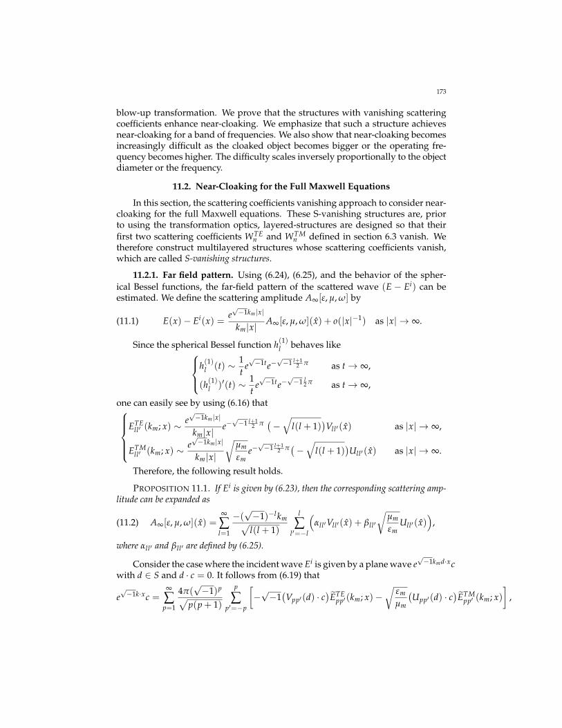
173

blow-up transformation. We prove that the structures with vanishing scatteringcoefficients enhance near-cloaking. We emphasize that such a structure achievesnear-cloaking for a band of frequencies. We also show that near-cloaking becomesincreasingly difficult as the cloaked object becomes bigger or the operating fre-quency becomes higher. The difficulty scales inversely proportionally to the objectdiameter or the frequency.

11.2. Near-Cloaking for the Full Maxwell Equations

In this section, the scattering coefficients vanishing approach to consider near-cloaking for the full Maxwell equations. These S-vanishing structures are, priorto using the transformation optics, layered-structures are designed so that theirfirst two scattering coefficients WTE

n and WTMn defined in section 6.3 vanish. We

therefore construct multilayered structures whose scattering coefficients vanish,which are called S-vanishing structures.

11.2.1. Far field pattern. Using (6.24), (6.25), and the behavior of the spher-ical Bessel functions, the far-field pattern of the scattered wave (E − Ei) can beestimated. We define the scattering amplitude A∞[ε, µ, ω] by

(11.1) E(x)− Ei(x) =e√−1km |x|

km|x|A∞[ε, µ, ω](x) + o(|x|−1) as |x| → ∞.

Since the spherical Bessel function h(1)l behaves likeh(1)l (t) ∼ 1

te√−1te−

√−1 l+1

2 π as t→ ∞,

(h(1)l )′(t) ∼ 1t

e√−1te−

√−1 l

2 π as t→ ∞,

one can easily see by using (6.16) thatETE

ll′ (km; x) ∼ e√−1km |x|

km|x|e−√−1 l+1

2 π(−√

l(l + 1))Vll′(x) as |x| → ∞,

ETMll′ (km; x) ∼ e

√−1km |x|

km|x|

√µm

εme−√−1 l+1

2 π(−√

l(l + 1))Ull′(x) as |x| → ∞.

Therefore, the following result holds.

PROPOSITION 11.1. If Ei is given by (6.23), then the corresponding scattering amp-litude can be expanded as

A∞[ε, µ, ω](x) =∞

∑l=1

−(√−1)−lkm√

l(l + 1)

l

∑l′=−l

(αll′Vll′(x) + βll′

√µm

εmUll′(x)

),(11.2)

where αll′ and βll′ are defined by (6.25).

Consider the case where the incident wave Ei is given by a plane wave e√−1kmd·xc

with d ∈ S and d · c = 0. It follows from (6.19) that

e√−1k·xc =

∞

∑p=1

4π(√−1)p√

p(p + 1)

p

∑p′=−p

[−√−1(Vpp′(d) · c

)ETE

pp′(km; x)−√

εm

µm

(Upp′(d) · c

)ETM

pp′ (km; x)]

,

174

and therefore,

app′ = −4π(√−1)p+1√

p(p + 1)(Vpp′(d) · c) and bpp′ = −

4π(√−1)p√

p(p + 1)

√εm

µm(Upp′(d) · c).

Hence, the scattering amplitude, denoted by A∞[ε, µ, ω](c, d; x), is given by (11.2)with(11.3)

αll′ =∞

∑p=1

p

∑p′=−p

4π(√−1)p√

p(p + 1)

[−√−1(Vpp′(d) · c)WTE,TE

ll′ ,pp′ −√

εm

µm(Upp′(d) · c)WTE,TM

ll′ ,pp′

],

βll′ =∞

∑p=1

p

∑p′=−p

4π(√−1)p√

p(p + 1)

[−√−1(Vpp′(d) · c)WTM,TE

ll′ ,pp′ −√

εm

µm(Upp′(d) · c)WTM,TM

ll′ ,pp′

],

which shows that the scattering coefficients appear in the expansion of the scatter-ing amplitude.

11.2.2. low frequency behavior of the scattering coefficients. The low fre-quency behavior of the scattering coefficients is now investigated. Let Γ(x) :=−1/(4π|x|) denote the fundamental solution corresponding to the case k = 0, andMD the associated boundary integral operator:

MD[ϕ](x) := p.v.ˆ

∂Dν(x)×

(∇x×

(Γ(x− y)ϕ(y)

))dσ(y), ϕ ∈ TH(div, ∂D).

Analogously to (6.7), one can prove that there is a unique solution (ϕ(0), ψ(0)) ∈TH(div, ∂D)× TH(div, ∂D) to the following equations:(11.4)(µ1 − µ0)

(µ1 + µ0

2(µ1 − µ0)I +MD

)0

0 (ε1 − ε0)

(ε1 + ε0

2(ε1 − ε0)I +MD

) [ ϕ(0)

ωψ(0)

]=

[Ei × ν

iHi × ν

]∣∣∣∣∂D

.

In fact, since ∂D is C1,α,MD is compact and one may apply the Fredholm altern-ative to prove unique solvability of above equation. Moreover, one has(11.5)‖ϕ(0)‖TH(div,∂D)+ω‖ψ(0)‖TH(div,∂D) ≤ C(‖Ei× ν‖TH(div,∂D)+ ‖Hi× ν‖TH(div,∂D)),

with a constant C = C(ε, µ).Let ρ be a small positive number and consider the boundary integral equation

(6.7) with k, k0, and ω replaced by ρk, ρk0, and ρω, respectively. Then, one has

MρkD −MD = O(ρ2), Mρk0

D −MD = O(ρ2),

andLρk

D −Lρk0D = O(ρ2).

Since(k2

2µ1+

k20

2µ0

)I +

k2

µ1Mk

D −k2

0µ0Mk0

D = ρ2ω2[

ε1 + ε0

2I + (ε1 − ε0)MD + O(ρ2)

],

if one expresses the solution (ϕ, ψ) to (6.7) as (’, ) := (’ρ, ρω ρ), then it satisfies(A + O(ρ)

) [ ϕρ

ρωψρ

]=

[Ei × ν

iHi × ν

]∣∣∣∣∂D

,

175

where A is the 2-by-2 matrix appeared in the left-hand side of (11.4). From theinvertibility of A, it follows that there are constants ρ0 and C = C(ε, µ, ω) inde-pendent of ρ as long as ρ ≤ ρ0 such that(11.6)‖ϕρ‖TH(div,∂D) + ρω‖ψρ‖TH(div,∂D) ≤ C

(‖Ei × ν‖TH(div,∂D) + ‖Hi × ν‖TH(div,∂D)

).

LEMMA 11.2. There exists ρ0 such that, for all ρ ≤ ρ0,∣∣∣WTE,TE(n,m)(p,q)[ε, µ, ρω]

∣∣∣ ≤ Cn+p

nn pp ρn+p+1,(11.7)

for all n, m, p, q ∈ N, where the constant C depends on (ε, µ, ω) but is independent of ρ.The same estimate holds for WTE,TM

(n,m)(p,q), WTM,TE(n,m)(p,q), and WTM,TM

(n,m)(p,q).

PROOF. Let (ϕ, ψ) be the solution to (6.7) with Ei(y) = ETEp,q(ρk0; y) and Hi =

− iρωµ0∇× Ei. Then, from (6.22), it follows that∥∥Ei,ρ∥∥

TH(div,∂D)+∥∥Hi,ρ∥∥

TH(div,∂D)≤ Cp

pp ρp,

where C is independent of ρ, and hence∥∥ϕρ∥∥

L2(∂D)+ ρ∥∥ψρ

∥∥L2(∂D)

≤ Cp

pp ρp,

for ρ ≤ ρ0 for some ρ0. So one gets (11.7) from the definition of the scatteringcoefficients in Definition 6.1.

11.2.3. S-vanishing Structures. We will use a multi-layer structure defined insection ?? to construct the near cloaking structure at low frequencies. In section6.3, using the symmetry of the layered radial structure, the scattering coefficientsare reduced to WTE

n and WTMn , given by (6.36) and (6.41).

To construct the S-vanishing structure at a fixed frequency ω, one looks for(µ, ε) such that

WTEn [ε, µ, ω] = 0, WTM

n [ε, µ, ω] = 0, n = 1, . . . , N,

for some N. More ambitiously one may look for a structure (µ, ε) for a fixed ωsuch that

WTEn [µ, ε, ρω] = 0, WTM

n [µ, ε, ρω] = 0for all 1 ≤ n ≤ N and ρ ≤ ρ0 for some ρ0. Such a structure may not exist. Soinstead one looks for a structure such that

(11.8) WTEn [µ, ε, ρω] = o(ρ2N+1), WTM

n [µ, ε, ρω] = o(ρ2N+1),

for all 1 ≤ n ≤ N and ρ ≤ ρ0 for some ρ0. Such a structure is called an S-vanishingstructure of order N at low frequencies. In the following subsection, the scatteringcoefficients are expanded at low frequencies and conditions for the magnetic per-meability and the electric permittivity to be an S-vanishing structure are derived.

Suppose that (µ, ε) is an S-vanishing structure of order N at low frequencies.Let the incident wave Ei be given by a plane wave e

√−1ρk·xc with |k| = k0(=

ω√

ε0µ0) and k · c = 0. From (11.3), the corresponding scattering amplitude,

176

A∞[µ, ε, ρω](c, k := k/|k|; x := x/|x|), is given by (11.2) with the following αn,mand βn,m:

αn,m =4π(√−1)n√

n(n + 1)(Vn,m(k) · c)WTE

n [µ, ε, ρω],

βn,m = −4π(√−1)n√

n(n + 1)1√−1ωµ0

(Un,m(k) · c)WTMn [µ, ε, ρω].

Applying (11.7) and (11.8),

(11.9) A∞[µ, ε, ρω](c, k; x) = o(ρ2N+1)

uniformly in (k, x) if ρ ≤ ρ0. Thus using such a structure, the visibility of scatter-ing amplitude is greatly reduced.

11.2.4. Asymptotic Expansion of the Scattering Coefficients. The sphericalBessel functions of the first and second kinds have the series expansions

jn(t) =∞

∑l=0

(−1)ltn+2l

2l l!1 · 3 · · · (2n + 2l + 1)

and

yn(t) = −(2n)!2nn!

∞

∑l=0

(−1)lt2l−n−1

2l l!(−2n + 1)(−2n + 3) · · · (−2n + 2l − 1).

So, using the notation of double factorials, which is defined by

n!! :=

n · (n− 2) . . . 3 · 1 if n > 0 is odd,n · (n− 2) . . . 4 · 2 if n > 0 is even,1 if n = −1, 0,

one has

(11.10) jn(t) =tn

(2n + 1)!!(1 + o(t)

)for t 1

and

(11.11) yn(t) = −((2n− 1)!!

)t−n+1(1 + o(t)

)for t 1.

One now computes PTEn [ε, µ, t] for small t. For n ≥ 1,

PTEn [ε, µ, t] = (−

√−1t)L

(L

∏j=1

µ32j ε

12j rj

) znL

(2n + 1)!!tn + o(tn)

−√−1Q(n)zn+1

Lt−n−1

0 0

×L

∏j=1

√−1Q(n)n

µj(zjrj)n+1 t−n−1 + o(t−n−1)

√−1Q(n)

(zjrj)n+1 t−n−1 + o(t−n−1)

−(n + 1)(zjrj)n

µj(2n + 1)!!tn + o(tn)

(zjrj)n

(2n + 1)!!tn + o(tn)

(zj−1rj)n

(2n + 1)!!tn + o(tn)

−√−1Q(n)

(zj−1rj)n+1 t−n−1 + o(t−n−1)

(n + 1)(zj−1rj)n

µj−1(2n + 1)!!tn + o(tn)

√−1Q(n)n

µj−1(zj−1rj)n+1 t−n−1 + o(t−n−1)

,

177

where zj =√

εjµj and Q(n) = (2n− 1)!!. One then has

PTEn [ε, µ, t] =

znL

(2n + 1)!!tn + o(tn)

−√−1Q(n)zn+1

Lt−n−1 + o(t−n−1)

0 0

×

L

∏j=1

Q(n)zn

j−1

(2n + 1)!!znj

(n +

(n + 1)µj

µj−1

)(1 + o(1)

)(−√−1)

(Q(n))2nzn

j zn+1j−1 r2n+1

j

(1−

µj

µj−1

)t−2n−1(1 + o(1)

)√−1

znj−1zn+1

j r2n+1j (n + 1)

((2n + 1)!!)2

(1−

µj

µj−1

)t2n+1(1 + o(1)

) Q(n)zn+1j

(2n + 1)!!zn+1j−1

(n + 1 +

nµj

µj−1

)(1 + o(1)

) .

Similarly, for the transverse magnetic case, one has

PTMn [ε, µ, t] =

(n + 1)znL

(2n + 1)!!tn + o(tn)

−√−1nQ(n)zn+1

Lt−n−1 + o(t−n−1)

0 0

×

L

∏j=1

Q(n)zn

j−1

(2n + 1)!!znj

((n +

εj

εj−1(n + 1)

)(1 + o(1)

)(−√−1)

(Q(n))2nzn

j zn+1j−1 r2n+1

j

(1−

εj

εj−1

)t−2n−1(1 + o(1)

)√−1

znj−1zn+1

j r2n+1j (n + 1)

((2n + 1)!!)2

(1−

εj

εj−1

)t2n+1(1 + o(1)

) Q(n)zn+1j

(2n + 1)!!zn+1j−1

(n + 1 +

εj

εj−1n

)(1 + o(1)

) .

Using the behavior of spherical Bessel functions for small arguments, one cansee that pTE

n,1 and pTEn,2 admit the following expansions:

(11.12) pTEn,1[µ, ε, t] = tn

(N−n

∑l=0

f TEn,l (µ, ε)t2l + o(t2N−2n)

)and

(11.13) pTEn,2[µ, ε, t] = t−n−1

(N−n

∑l=0

gTEn,l (µ, ε)t2l + o(t2N−2n)

).

Similarly, pTMn,1 and pTM

n,2 have the following expansions:

(11.14) pTMn,1 [µ, ε, t] = tn

(N−n

∑l=0

f TMn,l (µ, ε)t2l + o(t2N−2n)

)and

(11.15) pTMn,2 [µ, ε, t] = t−n−1

(N−n

∑l=0

gTMn,l (µ, ε)t2l + o(t2N−2n)

)for t = ρω and some functions f TE

n,l , gTEn,l , f TM

n,l , and gTMn,l independent of t.

LEMMA 11.3. For any pair of (µ, ε), one has

(11.16) gTEn,0(µ, ε) 6= 0

and

(11.17) gTMn,0 (µ, ε) 6= 0.

178

PROOF. Assume that there exists a pair of (µ, ε) such that gTEn,0(µ, ε) = 0. Since

pTEn,2[µ, ε, ρω] = o(ρ−n−1), the solution given by (6.29) with a0 = 1 and a0 = 0

satisfies ∇×

(1µ∇× E

)− ρ2ω2εE = 0 in R3 \ D,

∇ · E = 0 in R3 \ D,(ν× E)

∣∣+= o(ρ−(n+1)) on ∂D,

E(x) = h(1)n (ρk0|x|)Vn,0(x) for |x| > 2.

Let V(x) = limρ→0 ρn+1E(x). Using (11.11) one knows that the limit V satisfies∇×

(1µ∇×V

)= 0 in R3 \ D,

∇ ·V = 0 in R3 \ D,(ν×V)

∣∣+= 0 on ∂D,

V(x) = −((2n− 1)!!)Vn,0(x) for |x| > 2.

Since Vn,0(x) = O(|x|−1), one gets V(x) = 0 by Green’s formula, which is acontradiction. Thus gTE

n,0(µ, ε) 6= 0. In a similar way, (11.17) can be proved.

From Lemma 11.3, one obtains the following result.

PROPOSITION 11.4. One has

WTEn [µ, ε, t] = t2n+1

N−n

∑l=0

WTEn,l [µ, ε]t2l + o(t2N+1)

and

WTMn [µ, ε, t] = t2n+1

N−n

∑l=0

WTMn,l [µ, ε]t2l + o(t2N+1),

where t = ρω and the coefficients WTEn,l [µ, ε] and WTM

n,l [µ, ε] are independent of t.

Hence, if one has (µ, ε) such that

(11.18) WTEn,l [µ, ε] = WTM

n,l [µ, ε] = 0, for all 1 ≤ n ≤ N, 0 ≤ l ≤ (N − n),

(µ, ε) satisfies (11.8); in other words, it is an S-vanishing structure of order N at lowfrequencies. It is quite challenging to construct (µ, ε) analytically satisfying (11.18).The next subsection presents some numerical examples of such structures.

11.2.5. Numerical Implementation.

Code: 11.1 Near Cloaking for Maxwell’s Equations DemoNearCloaking.m

In this section we demonstrate some numerical examples of S-vanishing struc-tures of order N at low frequencies based on (11.18). As in the previous sections,we do this using a gradient descent method for a suitable energy functional. Wesymbolically compute the scattering coefficients. In the place of spherical Besselfunctions and spherical Hankel functions, we use their low-frequency expansionsand symbolically compute WTE

n and WTMn to obtain WTE

n,l and WTMn,l .

The following example is a S-vanishing structure of order N = 2 made of 6multilayers. The radii of the concentric disks are rj = 2 − j−1

6 for j = 1, . . . , 7.

http://www.sam.math.ethz.ch/~grsam/HS16/MCMP/Code/Tutorial11/11.1 Near Cloaking for Maxwell's Equations.zip

179

From Proposition 11.4, the nonzero leading terms of WTEn [µ, ε, t] and WTM

n [µ, ε, t]up to t5 are

• [t3, t5] terms in WTE1 [µ, ε, t], i.e., WTE

1,0 , WTE1,1 ,

• [t3, t5] terms in WTM1 [µ, ε, t], i.e., WTM

1,0 , WTM1,1 ,

• [t5] term in WTE2 [µ, ε, t], i.e., WTE

2,0 ,• [t5] term in WTM

2 [µ, ε, t], i.e., WTM2,0 .

Consider the mapping

(11.19) (µ, ε) −→ (WTE1,0 , WTE

1,1 , WTM1,0 , WTM

1,1 , WTE2,0 , WTM

2,0 ),

where, µ = (µ1, . . . , µ6) and ε = (ε1, . . . , ε6). One looks for (µ, ε) in which theright-hand side of (11.19) is as small as possible. Since (11.19) is a nonlinear equa-tion, we solve it iteratively. Initially, we set µ = µ(0) and ε = ε(0). We theniteratively modify (µ(i), ε(i))

(11.20) [µ(i+1) ε(i+1)]T = [µ(i) ε(i)]T − A†i b(i),

where A†i is the pseudoinverse of

Ai :=∂(WTE

1,0 , WTE1,1 , . . . , WTM

2,0 )

∂(µ, ε)

∣∣∣(µ,ε)=(µ(i),ε(i))

,

and

b(i) =

WTE

1,0WTE

1,1...

WTM2,0

∣∣∣∣∣∣∣∣∣(µ,ε)=(µ(i),ε(i))

.

Example 1. Figure 11.1 and Figure 11.2 show computational results for a 6-layer S-vanishing structure of order N = 2. We sets r = (2, 11

6 , . . . , 76 ), µ(0) = (3, 6, 3, 6, 3, 6)

and ε(0) = (3, 6, 3, 6, 3, 6) and modify them following (11.20) with the constraintsthat µ and ε belongs to the interval between 0.1 and 10. The obtained materialparameters are µ = (0.1000, 1.1113, 0.2977, 2.0436, 0.1000, 1.8260) andε = (0.4356, 1.1461, 0.2899, 1.8199, 0.1000, 3.1233), respectively. In contrast to theno-layer structure with PEC condition at |x| = 1, the obtained multilayer structurehas nearly zero coefficients for WTE

n [µ, ε, t] and WTMn [µ, ε, t] up to t5.

11.3. Enhancement of near cloaking

In this section we constructs a cloaking structure based on the following lemma.

LEMMA 11.5. Let F be an orientation-preserving diffeomorphism of R3 onto R3 suchthat F(x) is identity for |x| large enough. If (E, H) is a solution to

(11.21)

∇× E = iωµH in R3,∇× H = −iωεE in R3,(E− Ei, H − Hi) is radiating,

180

FIGURE 11.1. This figure shows the graph of the material para-meters and the corresponding coefficients in WTE

n [µ, ε, t] andWTM

n [µ, ε, t] up to t5. The first row is for the no-layer case, and thesecond row is for a 6-layer S-vanishing structure of order N = 2,which is explained in Example 1. In the third column, the y-axisshows (WTE

1,0 , WTE1,1 , WTM

1,0 , WTM1,1 , WTE

2,0 , WTM2,0 ) from left to right.

then (E, H) defined by (E(y), H(y)) =((DF)−TE(F−1(y)), (DF)−T H(F−1(y))

)sat-

isfies ∇× E = iω(F∗µ)H in R3,∇× H = −iω(F∗ε)E in R3,(E− Ei, H − Hi) is radiating,

where (Ei(y), Hi(y)) =((DF)−TEi(F−1(y)), (DF)−T Hi(F−1(y))

),

(F∗µ)(y) =DF(x)µ(x)DFT(x)

det(DF(x)), and (F∗ε)(y) =

DF(x)ε(x)DFT(x)det(DF(x))

,

with x = F−1(y) and DF is the Jacobian matrix of F.Hence,

A[µ, ε, ω] = A[F∗µ, F∗ε, ω].

To compute the scattering amplitude which corresponds to the material para-meters before the transformation, we consider the following scaling function, forsmall parameter ρ,

Ψ 1ρ(x) =

1ρ

x, x ∈ R3.

Then we have the following relation between the scattering amplitudes, whichcorrespond to two sets of differently scaled material parameters and frequency:

(11.22) A∞

[µ Ψ 1

ρ, ε Ψ 1

ρ, ω

]= A∞[µ, ε, ρω].

181

FIGURE 11.2. This figure shows the graph of WTEn [µ, ε, t] and

WTMn [µ, ε, t] for various values of t. The first row is for the no-

layer case, and the second row is for a 6-layer S-vanishing struc-ture of order N = 2 which is explained in Example 1. The valuesof WTE

n and WTMn are much smaller in the S-vanishing structure

than in the no-layer structure.

To see this, consider (E, H) which satisfies(∇× E) (x) = iω

(µ Ψ 1

ρ

)(x)H(x) for x ∈ R3 \ Bρ,

(∇× H) (x) = −iω(ε Ψ 1

ρ

)(x)E(x) for x ∈ R3 \ Bρ,

x× E(x) = 0 on ∂Bρ,(E− Ei, H − Hi) is radiating,

with the incident wave Ei(x) = eik·x c and Hi = 1iωµ0∇× Ei with k · c = 0 and

|k| = k0. Here Bρ is the ball of radius ρ centered at the origin. Set y = 1ρ x and

define(E(y), H(y)

):=((

E Ψ−11ρ

)(y),

(H Ψ−1

1ρ

)(y))=((

E Ψρ

)(y),

(H Ψρ

)(y))

and (Ei(y), Hi(y)

):=((

Ei Ψρ

)(y),

(Hi Ψρ

)(y))

.

182

Then, one has

(∇y × E

)(y) = iρωµ(y)H(y) for y ∈ R3 \ B1(

∇y × H)(y) = −iρωε(y)E(y) for y ∈ R3 \ B1,

y× E(y) = 0 on ∂B1,(E− Ei, H − Hi) is radiating

Recall that the scattered wave can be represented using the scattering amplitudeas follows:

(E− Ei)(x) ∼ eik0|x|

k0|x|A∞

[µ Ψ 1

ρ, ε Ψ 1

ρ, ω

](c, k; x) as |x| → ∞,

and

(E− Ei)(y) ∼ eik0ρ|y|

k0ρ|y| A∞ [µ, ε, ω] (c, k; x) as |y| → ∞.

Since the left-hand sides of the previous equations are coincident, we have (11.22).Suppose that (µ, ε) is an S-vanishing structure of order N at low frequencies

as in Section 11.2. From (11.9) and (11.22). Then we have

(11.23) A∞

[µ Ψ 1

ρ, ε Ψ 1

ρ, ω

](c, k; x) = o(ρ2N+1)

. We define the diffeomorphism Fρ as

Fρ(x) :=

x for |x| ≥ 2,( 3− 4ρ

2(1− ρ)+

14(1− ρ)

|x|) x|x| for 2ρ ≤ |x| ≤ 2,(1

2+

12ρ|x|) x|x| for ρ ≤ |x| ≤ 2ρ,

xρ

for |x| ≤ ρ.

Then using (11.23) and Lemma 11.5 we obtain the main result of this chapter.

THEOREM 11.6. If (µ, ε) is a S-vanishing structure of order N at low frequencies,then there exists ρ0 such that

A∞

[(Fρ)∗(µ Ψ 1

ρ), (Fρ)∗(ε Ψ 1

ρ), ω

](c, k; x) = o(ρ2N+1),

for all ρ ≤ ρ0, uniformly in (k, x).

Note that the cloaking structure((Fρ)∗(µ Ψ 1

ρ), (Fρ)∗(ε Ψ 1

ρ))

in Theorem

11.6 satisfies the PEC boundary condition on |x| = 1.

CHAPTER 12

Anomalous Resonance Cloaking and Shielding

12.1. Introduction

We consider the dielectric problem with a source term α f , proportional to f ,which models the quasi-static (zero-frequency) transverse magnetic regime. Thecloaking of the source is achieved in a region external to a plasmonic structure.The plasmonic structure consists of a shell having relative permittivity−1+

√−1δ

with δ modeling losses.The cloaking issue is directly linked to the existence of anomalous localized

resonance (ALR), which is tied to the fact that an elliptic system of equationscan exhibit localization effects near the boundary of ellipticity. The plasmonicstructure exhibits ALR if, as the loss parameter δ goes to zero, the magnitude ofthe quasi-static in-plane electric field diverges throughout a specific region (withsharp boundary not defined by any discontinuities in the relative permittivity),called the anomalous resonance region, but converges to a smooth field outsidethat region.

To state the problem, let Ω be a bounded domain in R2 and let D be a domainwhose closure is contained in Ω. Throughout this chapter, we assume that Ω andD are smooth. For a given loss parameter δ > 0, the permittivity distribution inR2 is given by

(12.1) εδ =

1 in R2 \Ω ,−1 +

√−1δ in Ω \ D ,

1 in D .

We may consider the configuration as a core with permittivity 1 coated by the shellΩ \ D with permittivity −1 +

√−1δ. For a given function f compactly supported

in R2 satisfying

(12.2)ˆ

R2f dx = 0

(which physically is required by conservation of charge), we consider the follow-ing dielectric problem:

(12.3) ∇ · εδ∇Vδ = α f in R2 ,

with the decay condition Vδ(x)→ 0 as |x| → ∞.A fundamental problem is to identify those sources f such that when α = 1

then first

(12.4) Eδ :=ˆ

Ω\Dδ|∇Vδ|2dx → ∞ as δ→ 0 .

183

184

and second Vδ remains bounded outside some radius a:

(12.5) |Vδ(x)| < C, when |x| > a

for some constants C and a independent of δ (which requires that the ball Ba con-tains the entire region of anomalous localized resonance). The quantity Eδ is pro-portional to the electromagnetic power dissipated into heat by the time harmonicelectrical field averaged over time. Hence (12.4) implies an infinite amount of en-ergy dissipated per unit time in the limit δ→ 0 which is unphysical. If instead wechoose α = 1/

√Eδ then the source α f will produce the same power independent

of δ and the new associated solution Vδ (which is the previous solution Vδ mul-tiplied by α) will approach zero outside the radius a: cloaking due to anomalouslocalized resonance (CALR) occurs. The conditions (12.4) and (12.5) are sufficientto ensure CALR: a necessary and sufficient condition is that (with α = 1) Vδ/

√Eδ

goes to zero outside some radius as δ → 0. We also consider a weaker blow-up ofthe energy dissipation, namely,

(12.6) lim supδ→0

Eδ = ∞ .

We say that weak CALR takes place if (12.6) holds (in addition to (12.5)). Thenthe (renormalized) source f /

√Eδ will be essentially invisible for an infinite se-

quence of small values of δ tending to zero (but would be visible for values of δinterspersed between this sequence if CALR does not additionaly hold).

The aim of this chapter is to review a general method based on the poten-tial theory to study cloaking due to anomalous resonance. Using layer potentialtechniques, we reduce the problem to a singularly perturbed system of integralequations. The system is non-self-adjoint. A symmetrization technique can be ap-plied in the general case. In the case of an annulus (D is the disk of radius ri and Ωis the concentric disk of radius re), it is known [?] that there exists a critical radius(the cloaking radius)

(12.7) r? =√

r3e ri−1 .

such that any finite collection of dipole sources located at fixed positions within theannulus Br? \ Be is cloaked. We show that if f is an integrable function supportedin E ⊂ Br? \ Be satisfying (12.2) and the Newtonian potential of f does not extendas a harmonic function in Br? , then weak CALR takes place. Moreover, we showthat if the Fourier coefficients of the Newtonian potential of f satisfy a mild gapcondition, then CALR takes place. Conversely we show that if the source functionf is supported outside Br? then (12.4) does not happen and no cloaking occurs.

We also show that a cylindrical superlens can also act as a new kind of elec-trostatic shielding device if the core is eccentric to the shell. While such a conven-tional device shields a region enclosed by the device, a superlens with an eccentriccore can shield a non-coated region which is located outside the device. Moreover,the size of the shielded region can be arbitrarily large while that of the device isfixed. We call this phenomenon shielding at a distance. The key element to study inthe eccentric case is the Möbius transformation via which a concentric annulus istransformed into an eccentric one. We also provide various numerical examplesto show the cloaking effect and shielding effect due to anomalous resonance.

185

12.2. Layer Potential Formulation

As in Chapter 2, for ∂D or ∂Ω, we denote, respectively, the single and doublelayer potentials of a function φ ∈ L2 as S0

D[φ] and D0Ω[φ]. We also introduce the

associated Neumann-Poincaré operators K0D and K0

Ω.Let F be the Newtonian potential of f , i.e.,

(12.8) F(x) =ˆ

R2Γ(x, y) f (y)dy, x ∈ R2 .

Then F satisfies ∆F = f in R2, and the solution Vδ to (12.3) may be represented as

(12.9) Vδ(x) = F(x) + S0D[φi](x) + S0

Ω[φe](x)

for some functions φi ∈ L20(∂D) and φe ∈ L2

0(∂Ω) (L20 is the collection of all square

integrable functions with the integral zero). The transmission conditions along theinterfaces ∂Ω and ∂D satisfied by Vδ read

(−1 +√−1δ)

∂Vδ

∂ν

∣∣∣+=

∂Vδ

∂ν

∣∣∣−

on ∂D ,

∂Vδ

∂ν

∣∣∣+= (−1 +

√−1δ)

∂Vδ

∂ν

∣∣∣−

on ∂Ω .

Hence the pair of potentials (φi, φe) is the solution to the following system of in-tegral equations:(−1 +

√−1δ)

∂S0D[φi]

∂νi

∣∣∣+− ∂S0

D[φi]

∂νi

∣∣∣−+ (−2 +

√−1δ)

∂S0Ω[φe]

∂νi= (2−

√−1δ)

∂F∂νi

on ∂D ,

(2−√−1δ)

∂S0D[φi]

∂νe+

∂S0Ω[φe]

∂νe

∣∣∣+− (−1 +

√−1δ)

∂S0Ω[φe]

∂νe

∣∣∣−= (−2 +

√−1δ)

∂F∂νe

on ∂Ω .

Note that we have used the notation νi and νe to indicate the outward normal on∂D and ∂Ω, respectively. Using the jump formula for the normal derivative of thesingle layer potentials, the above equations can be rewritten as

(12.10)

−zδ I + (K0D)∗ ∂

∂νiS0

Ω

∂

∂νeS0

D zδ I + (K0Ω)∗

[φiφe

]= −

∂F∂νi∂F∂νe

on L2

0(∂D)× L20(∂Ω), where we set

(12.11) zδ =

√−1δ

2(2−√−1δ)

.

Note that the operator in (12.10) can be viewed as a compact perturbation of theoperator

(12.12) Rδ :=

[−zδ I + (K0

D)∗ 0

0 zδ I + (K0Ω)∗

].

Recall that the eigenvalues of (K0D)∗ and (K0

Ω)∗ lie in the interval ] − 12 , 1

2 ].Observe that zδ → 0 as δ → 0 and that there are sequences of eigenvalues of(K0

D)∗ and (K0

Ω)∗ approaching 0 since (K0D)∗ and (K0

Ω)∗ are compact. So 0 is theessential singularity of the operator valued meromorphic function

λ ∈ C 7→ (λI + (K0Ω)∗)−1 .

186

This causes a serious difficulty in dealing with (12.10). We emphasize that (K0Ω)∗

is not self-adjoint in general. In fact, (K0Ω)∗ is self-adjoint only when ∂Ω is a circle

or a sphere.Let H = L2(∂D)× L2(∂Ω). We write (12.10) in a slightly different form. We

first apply the operator [−I 00 I

]: H → H

to (12.10). Then the equation becomes

(12.13)

zδ I − (K0D)∗ − ∂

∂νiS0

Ω

∂

∂νeS0

D zδ I + (K0Ω)∗

[φiφe

]=

∂F∂νi

− ∂F∂νe

.

Let the Neumann-Poincaré-type operator K∗ : H → H be defined by

(12.14) K∗ :=

−(K0D)∗ − ∂

∂νiS0

Ω

∂

∂νeS0

D (K0Ω)∗

,

and let

(12.15) Φ :=[

φiφe

], g :=

∂F∂νi

− ∂F∂νe

.

Then, (12.13) can be rewritten in the form

(12.16) (zδI + K∗)Φ = g ,

where I is given by

I =

[I 00 I

].

12.3. Explicit computations for an annulus

Let B be the disk of radius r0 is centered at the origin, then one can easily seethat for each integer n 6= 0

(12.17) S0B[e√−1nθ ](x) =

− r0

2|n|

(rr0

)|n|e√−1nθ if |x| = r < r0,

− r0

2|n|( r0

r

)|n|e√−1nθ if |x| = r > r0,

and hence

(12.18)∂

∂rS0

B[e√−1nθ ](x) =

−1

2

(rr0

)|n|−1e√−1nθ if |x| = r < r0,

12

( r0

r

)|n|+1e√−1nθ if |x| = r > r0.

187

We also get, for any integer n,

D0B[e√−1nθ ](x) =

12

(rr0

)|n|e√−1nθ if |x| = r < r0,

−12

( r0

r

)|n|e√−1nθ if |x| = r > r0.

It follows from (??) that

(12.19) (K0B)∗[e√−1nθ ] = 0 ∀n 6= 0.

As K0Ω[1] = 1/2, it follows that, when B is a disk, K0

B is a rank one operator whoseonly non-zero eigenvalue is 1/2. On the other hand, from K0

B[1] = 1/2 it alsofollows that

(12.20) S0B[1](x) =

ln r0 if |x| = r < r0,

ln |x| if |x| = r > r0,

and hence

(12.21)∂

∂rS0

B[1](x) =

0 if |x| = r < r0,1r

if |x| = r > r0.

Let Ωi and Ωe be two concentric disks in R2 with radii ri < re. Define (K0Ωe\Ωi

)∗

by

(12.22) (K0Ωe\Ωi

)∗ =

(−(K0

Ωi)∗ − ∂

∂νi S0Ωe

∂∂νe S0

Ωi(K0

Ωe)∗

),

where νi and νe are the outward normal vectors to ∂Ωi and Ωe, respectively. Letthe operator SΩe\Ωi

be given by

SΩe\Ωi=

(S0

ΩeS0

Ωi

∣∣∂Ωe

S0Ωe

∣∣∂Ωi

S0Ωi

).

Then, following the arguments given in Subsection ??, we can prove that (K0Ωe\Ωi

)∗

is compact and self-adjoint for the inner product(12.23)〈ϕ, ψ〉H∗ := −〈SΩe\Ωi

[ψ], ϕ〉1/2,−1/2 for ϕ, ψ ∈ H−1/2(∂Ωe)× H−1/2(∂Ωi).

The following lemma from [?] gives the eigenvalues and eigenvectors of theNeumann-Poincaré operator (K0

Ωe\Ωi)∗ associated with the circular shell Ωe \Ωi

onH∗.LEMMA 12.1. The eigenvalues of (K0

Ωe\Ωi)∗ onH∗ are

−12

,12

,−12(

rire)n,

12(

rire)n, n = 1, 2, . . . ,

and corresponding eigenvectors are[1− 1

re

],[

01

],

[e±√−1nθ

rire

e±√−1nθ

],

[e±√−1nθ

− rire

e±√−1nθ

], n = 1, 2, . . . .

188

PROOF. We first prove that ±1/2 are eigenvalues of (K0Ωe\Ωi

)∗ on H∗. From(12.21) we have

(K0Ωe\Ωi

)∗[

ab

]=

(− 1

2 01re

12

)[ab

],

where a and b are constants. So ±1/2 are eigenvalues of (K0Ωe\Ωi

)∗ onH∗.Now we consider (K0

Ωe\Ωi)∗ onH∗0 defined by

H∗0 := ϕ ∈ H∗ :< 1, ϕ >1/2,−1/2= 0.Because of (12.19) it follows that

(K0Ωe\Ωi

)∗ =

0 − ∂

∂νi S0Ωe

∂

∂νe S0Ωi

0

onH∗0 and hence we have from (12.18) that

(12.24) (K0Ωe\Ωi

)∗[

e√−1nθ

0

]=

12(

rire)|n|+1

[0

e√−1nθ

]and

(12.25) (K0Ωe\Ωi

)∗[

0e√−1nθ

]=

12(

rire)|n|−1

[e√−1nθ

0

]for all n 6= 0, which completes the proof of the lemma.

REMARK 12.2. From Lemma 12.1, it follows that the eigenvalues of (K0Ωe\Ωi

)∗

on H∗0 are ±(1/2)(ri/re)j and (K0Ωe\Ωi

)∗ as an operator on H∗ has the trivial ker-nel, i.e.,

(12.26) Ker (K0Ωe\Ωi

)∗ = 0.

12.4. Anomalous Resonance in an Annulus

In this section we consider the anomalous resonance when the domains Ωand D are concentric disks. We calculate the explicit form of the limiting solution.Throughout this section, we set Ω = Be = |x| < re and D = Bi = |x| < ri,where re > ri.

According to (12.24) and (12.25), if Φ is given by

Φ = ∑n 6=0

[φn

iφn

e

]e√−1nθ ,

then

K∗Φ = ∑n 6=0

ρ|n|−1

2φn

e

ρ|n|+1

2φn

i

e√−1nθ .

Thus, if g is given by

g = ∑n 6=0

[gn

ign

e

]e√−1nθ ,

189

the integral equations (12.16) are equivalent to

(12.27)

zδφn

i +ρ|n|−1

2φn

e = gni ,

zδφne +

ρ|n|+1

2φn

i = gne ,

for every |n| ≥ 1. It is readily seen that the solution Φ = (φi, φe) to (12.27) is givenby

φi = 2 ∑n 6=0

2zδgni − ρ|n|−1gn

e

4z2δ − ρ2|n| e

√−1nθ ,

φe = 2 ∑n 6=0

2zδgne − ρ|n|+1gn

i4z2

δ − ρ2|n| e√−1nθ .

If the source is located outside the structure, i.e., f is supported in R2 \ Be, thenthe Newtonian potential of f , F, is harmonic in Be and

(12.28) F(x) = c− ∑n 6=0

gne

|n|r|n|−1e

r|n|e√−1nθ ,

for |x| ≤ re, where g is defined by (12.15). Thus we have

(12.29) gni = −gn

e ρ|n|−1 .

Here, gne is the Fourier coefficient of − ∂F

∂νeon Γe, or in other words,

(12.30) − ∂F∂νe

= ∑n 6=0

gne e√−1nθ .

We then get

(12.31)

φi = −2 ∑

n 6=0

(2zδ + 1)ρ|n|−1gne

4z2δ − ρ2|n| e

√−1nθ ,

φe = 2 ∑n 6=0

(2zδ + ρ2|n|)gne

4z2δ − ρ2|n| e

√−1nθ .

Therefore, from (12.17) we find that(12.32)

S0D[φi](x) + S0

Ω[φe](x) = ∑n 6=0

2(r2|n|i − r2|n|

e )zδ

|n|r|n|−1e (4z2

δ − ρ2|n|)

gne

r|n|e√−1nθ , re < r = |x| ,

and

S0D[φi](x) = − ∑

n 6=0

r2|n|i (2zδ + 1)

|n|r|n|−1e (ρ2|n| − 4z2

δ)

gne

r|n|e√−1nθ , ri < r = |x| < re ,(12.33)

S0Ω[φe](x) = ∑

n 6=0

(2zδ + ρ2|n|)

|n|r|n|−1e (ρ2|n| − 4z2

δ)gn

e r|n|e√−1nθ , ri < r = |x| < re .(12.34)

We next obtain the following lemma which provides essential estimates forthe investigation of this section.

190

LEMMA 12.3. There exists δ0 such that

(12.35) Eδ :=ˆ

Be\Bi

δ|∇Vδ|2 ≈ ∑n 6=0

δ|gne |2

|n|( δ2

4 + ρ2|n|)

uniformly in δ ≤ δ0.

PROOF. Using (12.28), (12.33), and (12.34), one can see that

Vδ(x) = c + re ∑n 6=0

[r2|n|

ir|n|

(2zδ + 1)− (4z2δ + 2zδ)r|n|

]gn

e e√−1nθ

|n|r|n|e (4z2δ − ρ2|n|)

.

Then straightforward computations yield that

Eδ ≈ r2e ∑

n 6=0δ(1− ρ2|n|)

∣∣∣∣∣ 2zδ + 14z2

δ + ρ2|n|

∣∣∣∣∣2

(4|zδ|2 − ρ2|n|)|gn

e |2|n| .

If δ is sufficiently small, then one can also easily show that

|4z2δ − ρ2|n|| ≈ δ2

4+ ρ2|n| .

Therefore we get (12.35) and the proof is complete. We next investigate the behavior of the series in the right hand side of (12.35).

Let

(12.36) Nδ =ln(δ/2)

ln ρ.

If |n| ≤ Nδ, then (δ/2) ≤ ρ|n|, and hence

(12.37) ∑n 6=0

δ|gne |2

|n|( δ2

4 + ρ2|n|)≥ ∑

0 6=|n|≤Nδ

δ|gne |2

|n|( δ2

4 + ρ2|n|)≥ 1

2 ∑0 6=|n|≤Nδ

δ|gne |2

|n|ρ2|n| .

Suppose that

(12.38) lim sup|n|→∞

|gne |2

|n|ρ|n| = ∞.

Then there is a subsequence nk with |n1| < |n2| < · · · such that

(12.39) limk→∞

|gnke |2

|nk|ρ|nk |= ∞.

If we take δ = 2ρ|nk |, then Nδ = |nk| and

(12.40) ∑0 6=|n|≤Nδ

δ|gne |2

|n|ρ2|n| = ρ|nk | ∑0 6=|n|≤|nk |

|gne |2

|n|ρ2|n| ≥|g|nk |

e |2|nk|ρ|nk |

.

Thus we obtain from (12.35) that

(12.41) limk→∞

Eρ|nk | = ∞ .

We emphasize that (12.38) is not enough to guarantee (12.4). We now imposean additional condition for CALR to occur. We assume that gn

e satisfies the fol-lowing gap property:

191

GP : There exists a sequence nk with |n1| < |n2| < · · · such that

limk→∞

ρ|nk+1|−|nk | |gnke |2

|nk|ρ|nk |= ∞ .

If GP holds, then we immediately see that (12.38) holds, but the converse is nottrue. If (12.38) holds, i.e., there is a subsequence nk with |n1| < |n2| < · · · sat-isfying (12.39) and the gap |nk+1| − |nk| is bounded, then GP holds. In particular,if

(12.42) limn→∞

|gne |2

|n|ρ|n| = ∞ ,

then GP holds.Assume that gn

e satisfies GP and nk is such a sequence. Let δ = 2ρα forsome α and let k(α) be the number such that

|nk(α)| ≤ α < |nk(α)+1|.Then, we have(12.43)

∑0 6=|n|≤Nδ

δ|gne |2

|n|ρ2|n| = ρα ∑0 6=|n|≤α

|gne |2

|n|ρ2|n| ≥ ρ|nk(α)+1|−|nk(α) | |gnk(α)e |2

|nk(α)|ρ|nk(α) |→ ∞ ,

as α→ ∞.We obtain the following lemma.

LEMMA 12.4. If (12.38) holds, then

(12.44) lim supδ→0

Eδ = ∞ .

If gne satisfies the condition GP, then

(12.45) limδ→0

Eδ = ∞ .

Suppose that the source function is supported inside the radius r? =√

r3e r−1

i .Then its Newtonian potential cannot be extended harmonically in |x| < r? in gen-eral. So, if F is given by

(12.46) F = c− ∑n 6=0

anr|n|e√−1nθ , r < re ,

then the radius of convergence is less than r?. Thus we have

(12.47) lim sup|n|→∞

|n||an|2r2|n|? = ∞ ,

i.e., (12.38) holds. The GP condition is equivalent to that there exists nk with|n1| < |n2| < · · · such that

(12.48) limk→∞

ρ|nk+1|−|nk ||nk||ank |2r2|nk |? = +∞ .

The following is the main theorem of this section.

THEOREM 12.5. Let f be a source function supported in R2 \ Be and F be the New-tonian potential of f .

192

(i) If F does not extend as a harmonic function in Br? , then weak CALR occurs, i.e.,

(12.49) lim supδ→0

Eδ = ∞

and (12.5) holds with a = r2e /ri.

(ii) If the Fourier coefficients of F satisfy (12.48), then CALR occurs, i.e.,

(12.50) limδ→0

Eδ = ∞

and (12.5) holds with a = r2e /ri.

(iii) If F extends as a harmonic function in a neighborhood of Br? , then CALR doesnot occur, i.e.,

(12.51) Eδ < C

for some C independent of δ.

PROOF. If F does not extend as a harmonic function in Br? , then (12.38) holds.Thus we have (12.49). If (12.48) holds, then (12.50) holds by Lemma 12.4. Moreover,by (12.32), we see that

|Vδ| ≤ |F|+ ∑n 6=0

∣∣∣∣∣ 2(r2|n|i − r2|n|

e )zδ

|n|r|n|−1e (4z2

δ − ρ2|n|)

gne

r|n|

∣∣∣∣∣ ≤ |F|+ C ∑n 6=0

δr|n|e

( δ2

4 + ρ2|n|)|n|r|n|

≤ |F|+ C ∑n 6=0

r2|n|e

|n|r|n|i r|n|< C, if r = |x| > r2

eri

for some constants C which may differ at each occurrence.If F extends as a harmonic function in a neighborhood of Br? , then the power

series of F, which is given by (12.28), converges for r < r? + 2ε for some ε > 0.Therefore there exists a constant C such that

|gne |

|n|r|n|−1e

≤ C1

(r? + ε)|n|

for all n. It then follows that

(12.52) |gne | ≤ C(r2

e ρ−1 + reε)−|n|/2r|n|e ≤ (ρ−1 + ε)−|n|/2

for all n. This tells us that

∑n 6=0

δ|gne |2

|n|(δ2 + ρ2|n|)≤ ∑

n 6=0

|gne |2

2|n|ρ|n| ≤ ∑n 6=0

12|n|(1 + ερ)|n|

.

This completes the proof.

If f is a dipole in Br? \ Be, i.e., f (x) = a · ∇δy(x) for a vector a and y ∈ Br? \ Bewhere δy is the Dirac delta function at y. Then F(x) = a · ∇Γ(x, y). From thefollowing expansion of the fundamental solution of the Laplacian:

(12.53)(−1)|α|

α!∂αΓ(x, 0) =

−12π|α|

[a|α|α

cos |α|θr|α|

+ b|α|αsin |α|θ

r|α|

],

we have

(12.54) Γ(x, y) =∞

∑n=1

−12πn

[cos nθy

rny

rn cos nθ +sin nθy

rny

rn sin nθ

]+ C .

193

Then we see that the Fourier coefficients of F has the growth rate r−ny and satisfies

(12.48), and hence CALR takes place. Similarly CALR takes place for a sum ofdipole sources at different fixed positions in Br? \ Be.

If f is a quadrapole, i.e.,

f (x) = A : ∇∇δy(x) =2

∑i,j=1

aij∂2

∂xi∂xjδy(x)

for a 2× 2 matrix A = (aij) and y ∈ Br? \ Be. Then

F(x) =2

∑i,j=1

aij∂2Γ(x, y)

∂xi∂xj.

Thus CALR takes place. This is in agreement with the numerical result in [?].If f is supported in R2 \ Br? , then F is harmonic in a neighborhood of Br? , and

hence CALR does not occur by Theorem 12.5. In fact, we can say more about thebehavior of the solution Vδ as δ → 0 which is related to the observation in [?, ?]that in the limit δ → 0 the annulus itself becomes invisible to sources that aresufficiently far away.

THEOREM 12.6. If f is supported in R2 \ Br? , then (12.51) holds (with α = 1 in(12.3)). Moreover, we have

(12.55) sup|x|≥r?

|Vδ(x)− F(x)| → 0 as δ→ 0 .

PROOF. Since supp f ⊂ R2 \ Br? , the power series of F, which is given by(12.28), converges for r < r? + 2ε for some ε > 0.

According to (12.32), if re < r = |x|, then we have

Vδ(x)− F(x) = ∑n 6=0

2(r2|n|e − r2|n|

i )zδ

|n|r|n|−1e (ρ2|n| − 4z2

δ)

gne

r|n|e√−1nθ .

If |x| = r?, then the identity

(r2|n|e − r2|n|

i )zδ

|n|r|n|−1e (ρ2|n| − 4z2

δ)

gne

r|n|?=

(1− ρ2|n|)zδ

(ρ|n| − 4z2δρ−|n|)

gne r|n|?

|n|r|n|−1e

holds and ∣∣∣∣∣ (1− ρ2|n|)zδ

(ρ|n| − 4z2δρ−|n|)

∣∣∣∣∣ ≤∣∣∣∣∣ 1(z−1

δ ρ|n| − zδρ−|n|)

∣∣∣∣∣≤∣∣∣∣∣ 1=m(z−1

δ ρ|n| − zδρ−|n|)

∣∣∣∣∣ =(

δ

4 + δ2 ρ−|n| +1δ

ρ|n|)−1

.

It then follows from (12.52) that

|Vδ(x)− F(x)| ≤ 2 ∑n 6=0

(δ

4 + δ2 ρ−|n| +1δ

ρ|n|)−1 re

|n|

(ρ−1

ρ−1 + ε

)|n|/2

,

and hence|Vδ(x)− F(x)| → 0 as δ→ 0 .

194

Since Vδ − F is harmonic in |x| > re and tends to 0 as |x| → ∞, we obtain (12.55)by the maximum principle. This completes the proof.

Theorem 12.6 shows that any source supported outside Br? cannot make theblow-up of the power dissipation happen and is not cloaked. In fact, it is knownthat we can recover the source f from its Newtonian potential F outside Br? since fis supported outside Br? . Therefore we infer from (12.55) that f may be recoveredapproximately by observing Vδ outside Br? .

12.5. Shielding at a distance

In this section, we show that a cylindrical superlens can also act as a newkind of electrostatic shielding device if the core is eccentric to the shell. The his-torical root of electrostatic shielding reaches back to 1896 when Michael Faradaydiscovered that a region coated with a conducting material is not affected by ex-ternal electric fields. While such a conventional method shields a region enclosedby the device, a superlens with an eccentric core can shield a non-coated regionwhich is located outside the device. Moreover, the size of the shielded region canbe arbitrarily large while that of the device is fixed. We call this phenomenonshielding at a distance. The aim of this section is to investigate the conditions re-quired for shielding at a distance and geometric features such as the location andsize of the shielded region. The key element to study in the eccentric case is theMöbius transformation via which a concentric annulus is transformed into an ec-centric one. The electrostatic properties of the eccentric superlens can be derivedin a straightforward way from those of the concentric case since the Möbius trans-formation is a conformal mapping.

12.5.1. ALR of the concentric annulus. For convenience, we briefly reviewthe anomalous resonance caused by the concentric superlens whose geometry isdescribed in Figure 12.1(a).

We first fix some notations. We let Ωi and Ωe denote circular disks centeredat the origin with the radii ρi and ρe, respectively, satisfying 0 < ρi < ρe < 1.Identifying R2 as C, they can be represented as

Ωi =

z ∈ C : |z| < ρi

and Ωe =

z ∈ C : |z| < ρe

.

The core Ωi and the background R2 \Ωe are assumed to be occupied by the iso-tropic material of permittivity 1 and the shell Ωe \Ωi by the plasmonic materialof permittivity −1 + iδ with a given loss parameter δ > 0, i.e., the permittivitydistribution εδ is given by

(12.56) εδ =

1 in the core,−1 + iδ in the shell,1 in the background.

We also assume the annulus structure to be small compared to the operatingwavelength so that it can adopt the quasi-static approximation. Then the (quasi-static) electric potential Vδ satisfies

(12.57) ∇ · εδ∇Vδ = f in C,

where f represents an electrical source. We assume that f is a point multipolesource of order n located at a location z0 ∈ R2 \Ωe. Then the potential F generated

195

ε=1

ε=1

ε=-1+iδ

ρiρe

Ωi

Ωe

electric field ≈ 0

ρ*

Ω *critical region

point source

Ωi

Ωe

Ω b

FIGURE 12.1. Cloaking due to the anomalous localized reson-ance: (a) shows the structure of the superlens with concentric core;(b) illustrates the cloaking effect.

by the source f can be represented as

F(z) =n

∑k=1

Reck(z− z0)−k, z ∈ C,

with complex coefficients ck’s. When n = 1, the source f (or the potential F) meansa point dipole source.

Then the anomalous localized resonance can be summarized as follows.(i) the dissipation energy Wδ diverges as the loss parameter δ goes to zero if

and only if a point source f is located inside the region Ω∗ := |z| < ρ∗,where ρ∗ :=

√ρ3

e /ρi and Wδ is given by

(12.58) Wδ := Imˆ

R2εδ|∇Vδ|2 dx = δ

ˆΩe\Ωi

|∇Vδ|2.

Let us call Ω∗ (or ρ∗) the critical region (or the critical radius), respectively.(ii) the electric field −∇Vδ stays bounded outside some circular region re-

gardless of δ. More precisely, we have

(12.59) |∇Vδ(z)| ≤ C, z ∈ Ωb := |z| > ρ2e /ρi,

for some constant C independent of δ. Here, the subscript ‘b’ in Ωb indic-ates the boundedness of the electric field. Let us call Ωb the calm region.

12.5.2. Möbius transformation. In this section, we will show that the con-centric annulus can be transformed into an eccentric one by applying the Möbiustransformation Φ defined as

(12.60) ζ = Φ(z) := az + 1z− 1

with a given positive number a. We shall also discuss how the critical region istransformed depending on the ciritical paramter ρ∗.

The function Φ is a conformal mapping from C \ 1 to C \ a. It maps thepoint z = 1 to infinity, infinity to ζ = a, and z = 0 to ζ = −a. It maps a circlecentered at the origin, say Sρ := z ∈ C : |z| = ρ, to the circle given by

(12.61) Φ(Sρ) = z ∈ C : |z− c| = r, where c = aρ2 + 1ρ2 − 1

and r =2a

|ρ− ρ−1| .

196

-2 0 2

-3

-2

-1

0

1

2

3

original space, z-plane

ρ=1.5

ρ=2

ρ=2.5

ρ=1/1.5

ρ=1/2

ρ=1/2.5

ρ=1

-2 0 2

-3

-2

-1

0

1

2

3

transformed space, ζ - plane

ρ=1.5

ρ=2

ρ=2.5

ρ=1/1.5

ρ=1/2

ρ=1/2.5

ρ=1

a-a

FIGURE 12.2. The Möbius transformation Φ defined in (12.60)maps 0, ∞, 1 to −a, +a, ∞, respectively. The left figure showsradial coordinate curves |z| = ρ, ρ > 0, and the right figuretheir images transformed by Φ with a = 1. Concentric circles sat-isfying ρ 6= 1 are transformed into eccentric ones.

So the concentric circles Sρ’s with ρ 6= 1 are transformed to eccentric ones in ζ-plane; see Figure 12.2.

Let us discuss how the concentric superlens described in section 12.5.1 is geo-metrically transformed by the mapping Φ. Note that for 0 < ρ < 1, the trans-formed circle Φ(Sρ) always lies in the left half-plane of C. Since we assume that0 < ρi < ρe < 1, the concentric annulus in z-plane is changed to an eccentric onecontained in the left half ζ-plane. We let Ωi (or Ωe) denote the transformed disk ofΩi (or Ωe), respectively.

Now we consider the critical region Ω∗ = |z| < ρ∗ and the calm regionΩb. Let us denote the transformed critical region (or calm region) by Ω∗ (or Ωb),respectively. The shape of Ω∗ can be very different depending on the value of ρ∗.Suppose 0 < ρ∗ < 1 for a moment. Then the region Ω∗ is a circular disk containedin the left half ζ-plane. Next, assume that ρ∗ > 1. In this case, Ω∗ becomes theregion outside a disk which is disjoint from the eccentric annulus. Contrary to thecase when ρ∗ < 1, the region Ω∗ is now unbounded. Similarly, the shape of Ωbdepends on the paramter ρb := ρ2

e /ρi. If 0 < ρb < 1, Ωb is a region outside a circle.But, if ρb > 1, Ωb becomes a bounded circular region which does not intersect withthe eccentric superlens. This unbounded (or bounded) feature of the shape of Ω∗(or Ωb) will be essentially used to design a new shielding device.

12.5.3. Potential in the transformed space. Here, we will transform the po-tential Vδ via the Möbius map Φ and then show that the resulting potential de-scribes the physics of the eccentric superlens. Let us define the transformed poten-tial Vδ by Vδ(ζ) := Vδ Φ−1(ζ). Since the Möbius transformation Φ is a conformalmapping, it preserves the harmonicity of the potential and interface conditions. Itcan be easily shown that the transformed potential Vδ satisfies

(12.62) ∇ · εδ∇Vδ = f in C,

197

where f (ζ) = 1|Φ′ |2 ( f Φ−1)(ζ) and the permittivity εδ is given by

(12.63) εδ(ζ) =

1 in Ωi,

−1 + iδ in Ωe \ Ωi,1 in the background.

Therefore, the transformed potential Vδ represents the quasistatic electrical poten-tial of the eccentric superlens (12.63) induced by the source f (ζ).

Now we consider some physical properties in the transformed space. Thedissipation energy Wδ in the transformed space turns out to be the same as theoriginal one Wδ as follows:

Wδ = δ

ˆ∂(Ωe\Ωi)

Vδ∂Vδ

∂ndl = δ

ˆ∂(Ωe\Ωi)

Vδ1|Φ′|

∂Vδ

∂n|Φ′| dl = Wδ.(12.64)

In the derviation we have used the Green’s identity and the harmonicity of thepotentials Vδ and Vδ.

The point source f is transformed into another point source at a different loc-ation. To see this, we recall that the source f is located at z = z0 in the originalspace. It generates the potential F(z) = ∑n

k=1 Reck(z− z0)−k. By the map Φ, the

potential F becomes F := F Φ−1 which is of the following form:

(12.65) F(ζ) =n

∑k=1

Re

dn(ζ − ζ0)−k

,

where dk’s are complex constants and ζ0 := Φ(z0). So the transformed source f isa point multipole source of order n located at ζ = ζ0. It is also worth remarkingthat, if the point source f is located at z0 = 1 in the originial space, then f becomesa multipole source at infinity in the transformed space. In fact, its correspondingpotential F is of the following form:

F(ζ) =n

∑k=1

Re

ekζk

for some complex constants ek. For example, if n = 1, then the source f (or poten-tial F) represents a uniform incident field.

12.5.4. Shielding at a distance due to anomalous resonance. In this section,we analyze the anomalous resonance in the eccentric annulus and explain how anew kind of shielding effect can arise. In view of the previous section, the math-ematical description of anomalous resonance in the eccentric case can be directlyobtained from that in the concentric case as follows:

(i) the dissipation energy Wδ diverges as the loss parameter δ goes to zero ifand only if a point source f is located inside the region Ω∗.

(ii) the electric field −∇Vδ stays bounded in the calm region Ωb regardlessof δ, i.e.,

(12.66) |∇Vδ(ζ)| ≤ C, ζ ∈ Ωb,

for some constant C independent of δ.

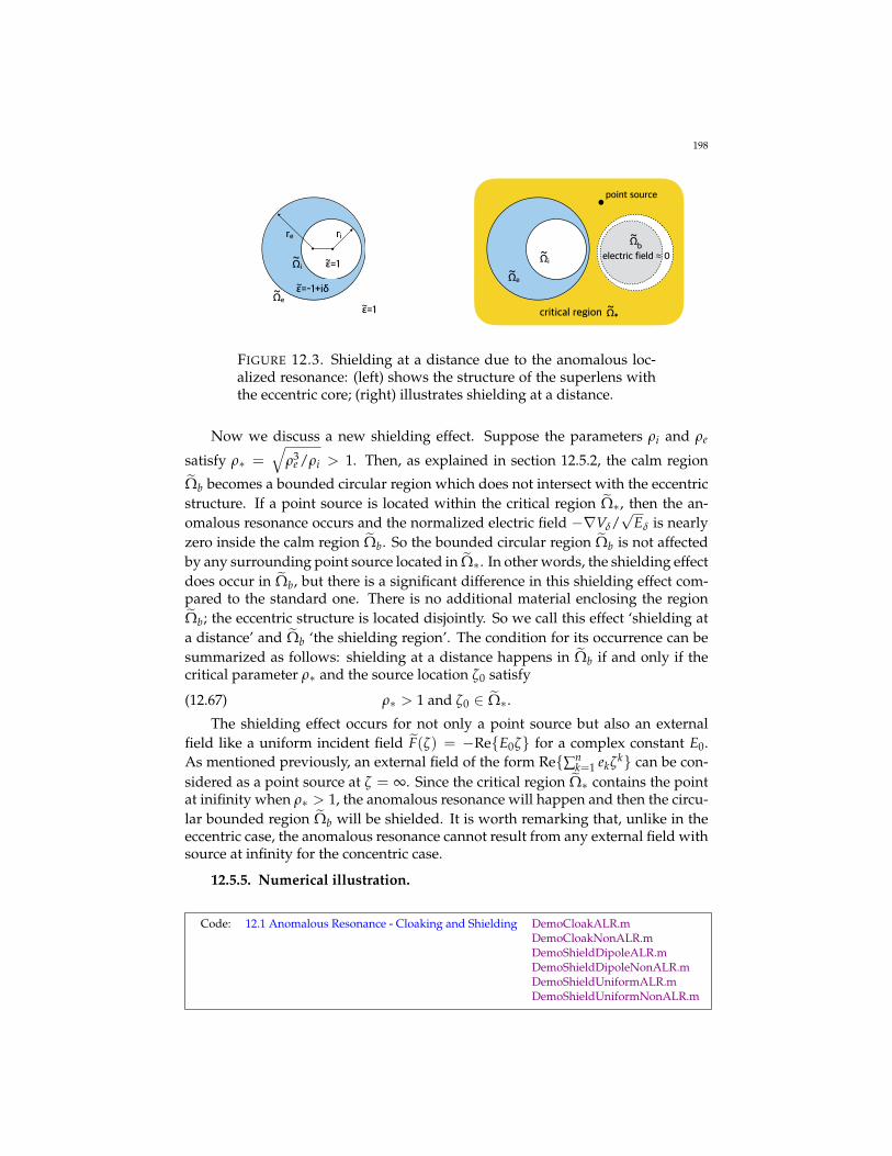
198

ε=1

ε=-1+iδ

ε=1

rire

Ωi

Ωe

~

~~

~

~Ω *critical region

point source

~

Ωi~

Ωe~

electric field ≈ 0

Ω b~

FIGURE 12.3. Shielding at a distance due to the anomalous loc-alized resonance: (left) shows the structure of the superlens withthe eccentric core; (right) illustrates shielding at a distance.

Now we discuss a new shielding effect. Suppose the parameters ρi and ρe

satisfy ρ∗ =√

ρ3e /ρi > 1. Then, as explained in section 12.5.2, the calm region

Ωb becomes a bounded circular region which does not intersect with the eccentricstructure. If a point source is located within the critical region Ω∗, then the an-omalous resonance occurs and the normalized electric field −∇Vδ/

√Eδ is nearly

zero inside the calm region Ωb. So the bounded circular region Ωb is not affectedby any surrounding point source located in Ω∗. In other words, the shielding effectdoes occur in Ωb, but there is a significant difference in this shielding effect com-pared to the standard one. There is no additional material enclosing the regionΩb; the eccentric structure is located disjointly. So we call this effect ‘shielding ata distance’ and Ωb ‘the shielding region’. The condition for its occurrence can besummarized as follows: shielding at a distance happens in Ωb if and only if thecritical parameter ρ∗ and the source location ζ0 satisfy

(12.67) ρ∗ > 1 and ζ0 ∈ Ω∗.

The shielding effect occurs for not only a point source but also an externalfield like a uniform incident field F(ζ) = −ReE0ζ for a complex constant E0.As mentioned previously, an external field of the form Re∑n

k=1 ekζk can be con-sidered as a point source at ζ = ∞. Since the critical region Ω∗ contains the pointat inifinity when ρ∗ > 1, the anomalous resonance will happen and then the circu-lar bounded region Ωb will be shielded. It is worth remarking that, unlike in theeccentric case, the anomalous resonance cannot result from any external field withsource at infinity for the concentric case.

12.5.5. Numerical illustration.

Code: 12.1 Anomalous Resonance - Cloaking and Shielding DemoCloakALR.mDemoCloakNonALR.mDemoShieldDipoleALR.mDemoShieldDipoleNonALR.mDemoShieldUniformALR.mDemoShieldUniformNonALR.m

http://www.sam.math.ethz.ch/~grsam/HS16/MCMP/Code/Tutorial12/12.1 Anomalous Resonance - Cloaking and Shielding.zip

199

In this section we demonstrate shielding at a distance by showing several ex-amples of the field distribution generated by an eccentric annulus and a pointsource. To compute the field distribution, we use an analytic solution derived byapplying a separation of variables method in polar coordinates to the concentriccase and then using the Möbius transformation Φ.

For all the examples below, we fix ρe = 0.7 for the concentric shell and a = 1for the Möbius transformation. We also fix the loss parameter as δ = 10−12.

Example 1 (Cloaking of a dipole source) We first present an eccentric annuluswhich acts as a cloaking device (Figure 12.4). Since we want to make a ‘cloaking’device, we need ρb to satisfy the condition ρb < 1. Setting ρi = 0.55 for thisexample, we have ρb = ρ2

e /ρi = 0.89 < 1 (ρ∗ = (ρ3e /ρi)

1/2 = 0.79). Then byapplying the Möbius transformation Φ, the concentric annulus is transformed tothe following eccentric structure from (12.61): the outer region Ωe = Φ(Ωe) is thecircular disk of radius 2.75 centered at (−2.92, 0) and the core Ωi = Φ(Ωi) is ofradius 1.58 centered at (−1.87, 0). The boundaries of the physical regions ∂Ωi and∂Ωe are plotted as solid white curves in Figure 12.4. On the other hand, the criticalregion’s boundary ∂Ω∗, which is not a material interface, and is the circle of radius4.08 centered at (−4.55, 0), is plotted as a dashed white circle. We refrain fromploting the calm region’s boundary ∂Ωb in the figure for the sake of the simplicity;it is relatively close to ∂Ω∗. Note that the calm region Ωb is an unbounded regionwhose boundary is slightly outside of ∂Ω∗.

In Figure 12.4(a), we assume that a dipole source F(ζ) = <b(ζ − ζ0)−1 is

located at ζ0 = (−3.4, 8.5) with the dipole moment b = (3,−3). The point sourceis plotted as a small solid disk (in white). It is clearly seen that the field distributionis smooth over the entire region except at the dipole source. That is, the anomal-ous resonance does not occur. We can detect the dipole source by measuring theperturbation of the electric field.

In Figure 12.4(b), we change the location of the source to ζ0 = (−3.4, 3.5) sothat the source’s location belongs to the critical region Ω∗. Then the anomalousresonance does occur, as shown in the figure. As a result, the potential ouside thewhite dashed circle becomes nearly constant. In other words, the dipole source isalmost cloaked.

Example 2 (Shielding at a distance for a dipole source) Next we show thatchanging the size of the core allows for shielding at a distance to happen for adipole source (Figure 12.5).

In Figure 12.5(a), we set ρi = 0.55 as in Example 1. We also assume that adipole source F(ζ) = <b(ζ − ζ0)

−1 is located at ζ0 = (5, 5) with the dipolemoment b = (3, 3). Since the source is located outside the critical region, theanomalous resonance does not happen.

Now let us change the size of the core. To make the shielding at distance occur,the critical radius ρ∗ satisfies the condition ρ∗ > 1. We set ρi = 0.2 so that ρ∗ =√

ρ3e /ρi = 1.31 > 1. Then, the core Ωi = Φ(Ωi) becomes the circular disk of radius

0.42 centered at (−1.08, 0). The critical region Ω∗ becomes the region outside thecircle of radius 3.53 centered at (4.06, 0). The resulting eccentric annulus and thecritical region are illustrated in Figure 12.5(b). Note that the source is containedin the new critical region Ω∗ and ρ∗ > 1. In other words, the condition (12.67)

200

FIGURE 12.4. Cloaking for a dipole source. We set ρi = 0.55,ρe = 0.7 and a = 1. The dipole source is located at ζ0 = (−3.4, 8.5)in the left figure and at ζ0 = (−3.4, 3.5) in the right figure. (left) Adipole source (small solid disk in white) is located outside the crit-ical region Ω∗ (white dashed circle). The field outside Ω∗ is signi-ficantly perturbed by the source. (right) A dipole source is locatedinside the critical region Ω∗. The anomalous resonance happensnear the superlens but the field outside Ω∗ becomes nearly zero.The source becomes almost cloaked. The plot range is from −10(blue) to 10 (red).

for shielding at a distance is satisfied. Indeed, inside the white dashed circle, thepotential becomes nearly constant while there is an anomalous resonance outside.Thus, sheiding at a distance occurs.

Example 3 (Shielding at a distance for a uniform field) Finally, we considershielding at a distance for a uniform field (Figure 12.6). We keep the parametersa, ρi and ρe as in the previous example but change the dipole source to a uniformfield F(ζ) = −<E0ζ with E0 = 1. As mentioned previously, an external fieldcan be considered as a point source located at infinity.

In the left figure, the critical region does not contain infinity. So the anomalousresonance does not happen. The uniform field can be easily detected. In the rightfigure, we changed the core as in the previous example. Now the critical region(the region outside the white dashed circle) does contain infinity. So the anomal-ous resonance does happen. Again, the potential becomes nearly constant in theregion inside the dashed circle. This means there is shielding at a distance for auniform field.

201

FIGURE 12.5. Shielding at a distance for a dipole source. We setρe = 0.7, a = 1 and ζ0 = (5, 5). We also set ρi = 0.55 in the leftfigure and ρi = 0.2 in the right figure. (left) The critical region Ω∗(white dashed line) contains the eccentric superlens (white solidlines). The field outside the white dashed circle is significantlyperturbed by the source. (right) The critical region is now theregion outside the white dashed circle which no longer containsthe superlens. The field inside the white dashed circle is nearlyzero and so shielding occurs. The plot range is from −10 (blue) to10 (red).

202

FIGURE 12.6. Shielding at a distance for a uniform field. We setρe = 0.7 and a = 1. We also set ρi = 0.55 in the left figureand ρi = 0.2 in the right figure. (left) The critical region Ω∗(white dashed line) contains the eccentric superlens (white solidlines). The uniform incident field is nearly unperturbed outsidethe white dashed circle. (right) The critical region Ω∗ is the re-gion outside the white dashed circle which does not contain thesuperlens any longer. The field inside the white dashed circle isnearly zero and so shielding occurs. The plot range is from −15(blue) to 15 (red).

Bibliography

[1] Atkinson, Kendall, and Weimin Han. "Numerical Solution of Fredholm Integral Equations of theSecond Kind." Cambridge University Press, 2009.

[2] Kress, Rainer, V. Maz’ya, and V. Kozlov. Linear integral equations. Vol. 17. Berlin: Springer-Verlag,1989.

[3] Klöckner, Andreas, et al. "Quadrature by expansion: A new method for the evaluation of layerpotentials." Journal of Computational Physics 252, 332-349, 2013.

203

Date post:	04-Apr-2019
Category:	Documents
Upload:	vanliem
View:	216 times
Download:	0 times

Mathematical and Computational Methods in Photonicsgrsam/HS17/MaCMiPaP... · 2017-10-24 ·...

Documents