WEB3GCH02 11/30/2013 10:2:37 Page 19

2 The use of correlation, association andregression to analyse processes and products

Daniel Cozzolino

School of Agriculture, Food and Wine, Faculty of Sciences, The University of Adelaide,Waite Campus, Glen Osmond, SA, Australia

ABSTRACT

No single technique can solve all analytical issues in the food processing industries. However, moderninstrumental techniques such as visible (Vis), near infrared (NIR), and mid infrared (MIR) spectroscopy,electronic noses (EN), electronic tongues (ET) and other sensors (e.g. temperature, pressure) combinedwith multivariate data analysis (MVA) have many advantages over chemical, physical and other classicinstrumental methods of analysis. This chapter provides a general description of the methods andapplications of regression analysis based onMVA used during the process analysis in the food industries.Most of the examples and applications given in this chapter are related with the use of infraredspectroscopy. However, the same basic principles can be applied to a different number of methods andinstruments currently used by the food industry.

INTRODUCTION

No single technique can solve all analytical issues in the food processing industries. However, moderninstrumental techniques such as visible (Vis), near infrared (NIR), and mid infrared (MIR) spectroscopy,electronic noses (EN), electronic tongues (ET) and other sensors (e.g. temperature, pressure) have manyadvantages over chemical, physical and other classic instrumental methods of analysis (Arvantoyanniset al., 1999; Blanco and Villaroya, 2002; McClure, 2003; Cozzolino et al., 2006a, 2011a, 2011b;Cozzolino, 2007, 2009, 2010, 2011, 2012; Roggo et al., 2007; Hashimoto and Kameoka, 2008; Huanget al., 2008; Cozzolino and Murray, 2012). Traditionally, much of the research into analytical and foodchemistry has been conducted in a manner that can be described as ‘univariate’ in nature, since it wasfocused only into the examination of the effects (responses) of a single variable on the overall matrix(Munck et al., 1998; Jaumot et al., 2004; Cozzolino and Murray, 2012). At the time that many statisticalmethods were developed around the 1920s (Bendell et al., 1999), samples were considered cheap andmeasurements expensive. Since that time, the nature of technology has changed; at present, samples areconsidered expensive while measurements cheap (Gishen et al., 2005; Cozzolino and Murray, 2012).

The analysis of the effects of onevariable at a time by the application of classical statistical analysis (e.g.analysis of variance) can provide useful descriptive information. However, specific information aboutrelationships among variables and other important relationships in the entire matrix might be lost (Wold,1995; Martens and Martens, 2001; Munck, 2007; Munck et al., 2010). Multivariate analysis (MVA) orchemometricswasdeveloped in the late 1960s, and introduced byanumberof researchgroups in chemistry,

Mathematical and Statistical Methods in Food Science and Technology, First Edition.Edited by Daniel Granato and Gast�on Ares.� 2014 John Wiley & Sons, Ltd. Published 2014 by John Wiley & Sons, Ltd.

WEB3GCH02 11/30/2013 10:2:37 Page 20

mainly in the fields of analytical, physical and organic chemistry, in order to deal with the introduction ofinstrumentation, which providesmultiple responses (e.g. peaks, wavelengths) for each sample analysed, aswell as with the increasingly availability and use of computers (Wold, 1995; Munck et al., 1998; Otto,1999). With modern chemical measurements, we are often confronted with so much data that the essentialinformation might not be readily evident. Certainly that can be the case with chromatographic or spectraldata for whichmany different observations (peaks or wavelengths) have been collected in a single analysis(Wold, 1995; Munck et al., 1998; Otto, 1999; Munck and Moller, 2011).

Traditionally as analysts, we strive to eliminate matrix interference in our methods by isolating orextracting the analyte we wish to measure, making the measurement apparently simple and certain(Wold, 1995; Munck et al., 1998; Otto, 1999). However, this scientific approach ignores the possibleeffects of chemical and physical interactions between the large amounts of constituents present in thesample – this will be especially evident for such complex materials as food. Univariate models do notconsider the contributions of more than one variable source and can result in models that could be anoversimplification (Wold, 1995; Munck et al., 1998; Otto, 1999). Therefore, we need to look at thesample in its whole and not just at a single component if we wish to unravel all the complicatedinteractions between the constituents as well as to understand their combined effects on the whole matrix(Wold, 1995; Geladi, 2003). Multivariate methods provide the means to move beyond the one-dimensional (univariate) world (Wold, 1995; Geladi, 2003). In many cases, MVA can reveal constituentsthat are important through the various interferences and interactions (Wold, 1995; Geladi, 2003). Today,many food quality measurement techniques are multivariate and based on indirect measurements of thechemical and physical properties by the application of modern instrumental methods and techniques(Esbensen, 2002; Geladi, 2003; Hashimoto and Kameoka, 2008; Woodcock et al., 2008; Blanco andBernardez, 2009; Cozzolino and Murray, 2012).

A typical characteristic of many of the most useful of these instrumental techniques is that,paradoxically, the measurement variable might not have a direct relationship with the property ofinterest; for instance, the concentration of a particular chemical in the sample – that is, the technique is acorrelative method. The explanation for this is often found in chemical and physical interferences. Forexample spectroscopy techniques provide the possibility to obtain more information from a singlemeasurement, because they can record responses at many wavelengths simultaneously, and it becomesessential to use MVA in order to extract the information. Specific details of the numerous algorithms,formulas and procedures used in multivariate analysis can be found in more specialized literature(Massart et al., 1988; Wold, 1995; Munck et al., 1998; Otto, 1999; Esbensen, 2002; Geladi, 2003; Markand Workman, 2003).

This chapter provides a general description of themethods and applications of regression analysis basedon multivariate data analysis used during the process analysis in the food industries. Most of the examplesand applications given are related to the use of infrared spectroscopy. However, the same basic principlescan be applied to a different number of methods and instruments currently used by the food industry.

PROCESS ANALYSIS

Over the past 30 years, on/in/at line analysis, the so called process analytical technologies (PAT), hasprovided to be one of the most efficient and advanced tools for continuous monitoring, controlling theprocesses and the quality of raw ingredients and products in several fields, including food processing,petrochemical and pharmaceutical industries (Beebe et al., 1993; Workman et al., 1999, 2001; Liu et al.,2001; Blanco and Villaroya, 2002; Huang et al., 2008; Karande et al., 2010). In this new context thesample becomes an integral component of the system (Figure 2.1). We are moving from the laboratory tothe process (Esbensen, 2002; Kueppers and Haider, 2003).

20 Mathematical and statistical methods in food science and technology

WEB3GCH02 11/30/2013 10:2:37 Page 21

Numerous applications can be found on the use and implementation of instrumental methods such asthose based on infrared (IR), temperature, moisture, gas, and pressure sensors for on-line and at-lineanalysis. The PAT tools are categorized into four areas, namely multivariate data acquisition and analysistools, modern process analyser or process analytical tools, process and endpoint monitoring and controltools, and continuous improvement and knowledge management tools (Workman et al., 1999, 2001;Skibsted, 2005). On-line applications based on IR spectroscopy started around the end of the 1980s.They were developed primary due to the availability of fibre optics (Workman et al., 1999, 2001;Skibsted, 2005). Most of such applications were related with the control and monitoring of liquids,mainly because the application of fibre optics was easier to use with such type of samples. Simplesystems are also used based on single sensors that collect changes in temperature, pressure, pH and in themixture of gases, among others.

In today’s manufacturers environment there is an increasing need for real process analyticalchemistry. The driving force behind this transition from traditional laboratory analysis to processanalysis is the need for more repaid process control information, as well as economical, safety, andenvironmental factors (Workman et al. 1999, 2001; Skibsted, 2005). Therefore, complex or multiplexsystems (combination of several sensors) and techniques are used (Blanco and Villaroya, 2002;McClure,2003; Roggo et al., 2007; Blanco and Bernardez, 2009; Huang et al., 2008; Cozzolino, 2009). Theoverall requirements on the use of MVAmethods for on line applications are: (i) can be assembled in theproduction line and take place under realistic environment; (ii) early detection of possible failures;(iii) permanent monitoring of the conditions; and (iv) assessment of the conditions at any desired time(Roggo et al., 2007; Blanco and Bernardez, 2009; Huang et al., 2008).

MULTIVARIATE METHODS

Multivariate statistical techniques (or chemometrics) are therefore required to extract the information aboutthe attributes measured that is buried in the signal produced by the instrumental method applied (‘modelcalibration’). Essentially, this process involves regression techniques coupledwith pre-processingmethods(Brereton, 2000, 2008; Næs et al., 2002; Cozzolino et al., 2006a, 2011a, 2011b; Nicolai et al., 2007).In many applications, it is expensive, time consuming or difficult to measure a property of interest directly.Such cases require the analyst to predict something of interest based on related properties that are easier tomeasure (Næs et al., 2002; McClure, 2003; Nicolai et al., 2007; Cozzolino et al., 2006, 2011; Walsh and

Figure 2.1 Sampling: from the laboratory to the ‘real world’. Adapted from Kuppers & Haider, 2003.

The use of correlation, association and regression to analyse processes and products 21

WEB3GCH02 11/30/2013 10:2:38 Page 22

Kawano, 2009). Hence, the goal of MVA regression analysis is to develop a calibration model whichcorrelates the information in the set of known measurements to the desired property.

Calibration is the process by which the mathematical relationship between the values provided by ameasuring instrument or system and those known for the measured material object is established. Themathematical expression relating analytical responses or signals to concentrations is known as thecalibration equation or calibration model (Mark and Workman, 2003; Blanco and Bernardez, 2009).Most analytical techniques use a straight line for calibration on account of its straightforward equationand its ability to illustrate a direct relationship between measured signals and concentrations (univariatecalibration) (Mark and Workman, 2003; Blanco and Bernardez, 2009). However, a linear calibrationmodel can only be useful for quantitation purposes if the analytical signal depends exclusively on theconcentration of the specific analyte for which the model has been developed. Such exclusivedependence is the exception rather than the rule in the analysis of complex samples by spectroscopictechniques, such as IR spectroscopy, as well as in other instrumental analytical methods (Mark andWorkman, 2003; Nicolai et al., 2007; Blanco and Bernardez, 2009).

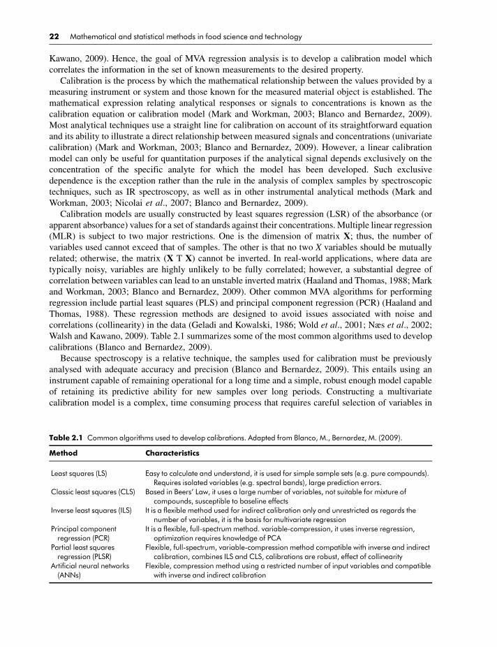
Calibration models are usually constructed by least squares regression (LSR) of the absorbance (orapparent absorbance) values for a set of standards against their concentrations. Multiple linear regression(MLR) is subject to two major restrictions. One is the dimension of matrix X; thus, the number ofvariables used cannot exceed that of samples. The other is that no two X variables should be mutuallyrelated; otherwise, the matrix (X T X) cannot be inverted. In real-world applications, where data aretypically noisy, variables are highly unlikely to be fully correlated; however, a substantial degree ofcorrelation between variables can lead to an unstable inverted matrix (Haaland and Thomas, 1988; Markand Workman, 2003; Blanco and Bernardez, 2009). Other common MVA algorithms for performingregression include partial least squares (PLS) and principal component regression (PCR) (Haaland andThomas, 1988). These regression methods are designed to avoid issues associated with noise andcorrelations (collinearity) in the data (Geladi and Kowalski, 1986; Wold et al., 2001; Næs et al., 2002;Walsh and Kawano, 2009). Table 2.1 summarizes some of the most common algorithms used to developcalibrations (Blanco and Bernardez, 2009).

Because spectroscopy is a relative technique, the samples used for calibration must be previouslyanalysed with adequate accuracy and precision (Blanco and Bernardez, 2009). This entails using aninstrument capable of remaining operational for a long time and a simple, robust enough model capableof retaining its predictive ability for new samples over long periods. Constructing a multivariatecalibration model is a complex, time consuming process that requires careful selection of variables in

Table 2.1 Common algorithms used to develop calibrations. Adapted from Blanco, M., Bernardez, M. (2009).

Method Characteristics

Least squares (LS) Easy to calculate and understand, it is used for simple sample sets (e.g. pure compounds).Requires isolated variables (e.g. spectral bands), large prediction errors.

Classic least squares (CLS) Based in Beers’ Law, it uses a large number of variables, not suitable for mixture ofcompounds, susceptible to baseline effects

Inverse least squares (ILS) It is a flexible method used for indirect calibration only and unrestricted as regards thenumber of variables, it is the basis for multivariate regression

Principal componentregression (PCR)

It is a flexible, full-spectrum method. variable-compression, it uses inverse regression,optimization requires knowledge of PCA

Partial least squaresregression (PLSR)

Flexible, full-spectrum, variable-compression method compatible with inverse and indirectcalibration, combines ILS and CLS, calibrations are robust, effect of collinearity

Artificial neural networks(ANNs)

Flexible, compression method using a restricted number of input variables and compatiblewith inverse and indirect calibration

22 Mathematical and statistical methods in food science and technology

WEB3GCH02 11/30/2013 10:2:38 Page 23

order to ensure accurate prediction of unknown samples. This requires knowledge not only of the targetsamples but also of MVA techniques, in order to obtain a model retaining its predictive ability over timeand amenable to easy updating. Because the model will usually be applied by unskilled operators, itshould deliver analytical information in an easily interpreted manner (Blanco and Bernardez, 2009). Theprocess of obtaining a robust model involves the following steps:

(i) choosing the samples for inclusion in the calibration set;(ii) determining the property to be predicted by using an appropriate method to measure such samples;(iii) obtaining the analytical instrumental signal (e.g. spectra);(iv) constructing the model;(v) validation;(vi) pre-processing of the data;(vii) prediction of unknown samples.

Selection of calibration samples is one of the most important steps in constructing a calibration modeland involves choosing a series of samples, which ideally should encompass all possible sources ofphysical and chemical variability in the samples to be subsequently predicted (Blanco and Bernardez,2009). The model will only operate accurately if both the calibration samples and the prediction samplesbelong to the same population. Usually, the set or population of available samples is split into twosubsets, called the calibration set (used to construct the model) and the validation set (Næs et al., 2002;McClure, 2003; Cozzolino et al., 2006a, 2011a, 2011b; Nicolai et al., 2007; Walsh and Kawano, 2009).The samples included in the calibration set should span the whole variability in both calibration andvalidation; thus, the selected samples should be uniformly distributed throughout the calibration range inthe multidimensional space defined by spectral variability. One simple method for selecting samplesbased on spectral variability uses a scatter plot obtained from a principal component analysis (PCA)applied to the whole set of available spectra. Inspecting the most significant PCs in the graph allows thedistribution of the sample spectra to be clearly envisaged; those to be included in the calibration set arechosen from both the extremes and the middle of the score maps obtained and simultaneously checked touniformly encompass the range spanned by the quantity to be determined (Figure 2.2). This method iseffective when the first two or three PCs contain a high proportion of the total variance (Mark, 1991;Fearn, 1997, 2002; Næs et al., 2002; McClure, 2003; Cozzolino et al., 2006a, 2006b, 2011a, 2011b;Nicolai et al., 2007; Blanco and Bernardez, 2009; Walsh and Kawano, 2009). As a rule of thumb,samples used to build a calibration model should be selected from samples similar to those that will beanalysed in the future (Murray, 1993, 1999; Murray and Cowe, 2004). The calibration samples should besubjected exactly to the same handling process to be adopted with future samples. It is also recom-mended to obtain the widest range in composition not only for the property of interest but for all sourcesof possible variation to be encounter in the future. Obtain sufficient extreme samples to emphasize thetail of the distribution (Murray, 1993, 1999; Murray and Cowe, 2004).

As previously described, before building a calibration model for a given analyte using spectra (e.g.NIR and MIR), a series of steps needs to be considered. Spectral pre-processing techniques are used toremove any irrelevant information that cannot be handled by the regression techniques. Several pre-processing methods have been developed for this purpose and several references can be found elsewhere(Brereton, 2000; Martens and Martens, 2000; Mark and Workman, 2003; Næs et al., 2002; Blanco andBernardez, 2000; Karoui et al., 2010). This can include averaging over spectra, which is used to reducethe number of wavelengths or to smooth the spectrum (Nicolai et al., 2007), moving average filters andthe Savitzky–Golay algorithm (Næs et al., 2002; Mark andWorkman, 2003; Nicolai et al., 2007; Blancoand Bernardez, 2009). Another pre-processing technique commonly used is standardization. Standard-ization means dividing the spectrum at every wavelength by the standard deviation of the spectrum at this

The use of correlation, association and regression to analyse processes and products 23

WEB3GCH02 11/30/2013 10:2:38 Page 24

wavelength. Typically variances of all wavelengths are standardized to one, which results in an equalinfluence of the variables in the model. Other standardization procedures are possible as well (Næs et al.,2002;Mark andWorkman, 2003; Blanco and Bernardez, 2009). Standardization is commonly used whenvariables are measured in different units or have different ranges. While most chemometrics softwarepackages offer several normalization methods, multiple scatter correction (MSC) and standard normalvariate correction (SNV), are the most popular normalization technique (Dhanoa et al., 1994; Næs et al.,2002; Mark and Workman, 2003; Blanco and Bernardez, 2009). MSC is used to compensate for additive(baseline shift) and multiplicative (tilt) effects in the spectral data, which are induced by physical effects(scattering, particle size and the refractive index) (Mark and Workman, 2003; Nicolai et al., 2007;Blanco and Bernardez, 2009). In SNV, each individual spectrum is normalized to zero mean and unitvariance (Dhanoa et al., 1994). Derivation is used to remove baseline shifts and superposed peaks(Duckworth, 2004; Næs et al., 2002).

OUTLIER DETECTION

Outliers may be induced by typing errors, file transfer, interface errors, sensor malfunctions and fouling,poor sensor calibration, bad sampling or sample presentation, among other factors. A sample can beconsidered as an outlier according to the X-variables only (spectra), to the Y-variables only (reference),or to both. It might also not be an outlier for either separate sets of variables but become an outlier whenthe X–Y relationship is considered. During calibration, outliers related to the spectra show up in agraphical scale or diagram called a PCA scores plot as points outside the normal range of variability.Alternatively, the leverage of a spectrum might be calculated as the distance to the centre of all spectrarelative to the variability in its particular direction. Additionally, X-residuals plots can be constructed. Y-outliers can be identified as extreme values in the Y-residuals plot. In practice, however, only thoseoutliers that have an effect on the regression model have to be removed (Adams, 1995; Wise andGallagher, 1996; Mark and Workman, 2003; Nicolai et al., 2007; Brereton, 2008; Cozzolino et al.,2011a, 2011b).

PC2

PC1

Step 1. Overview of dataOutlier detectionPatterns

Step 2. Pre-processingAlgorithm selectionValidation

Calibrationdevelopment

Step 3. Routine useValidationRe-calibration

Routine analysis andApplication

Figure 2.2 Steps during the application of multivariate data methods in food processing.

24 Mathematical and statistical methods in food science and technology

WEB3GCH02 11/30/2013 10:2:38 Page 25

MODEL ACCURACY AND VALIDATION

Once the calibration model has been developed, its ability to predict unknown samples not present in thecalibration set (e.g. not used to construct the model) should be assessed. This involves applying themodel to a limited number of samples not included in the calibration set, for which the target property tobe predicted by the model is previously known. The results provided by the model are directly comparedwith the reference values; if the two are essentially identical, the model will afford accurate predictionsand be useful for determining the target property in future (e.g. unknown samples). In order to assess theaccuracy of the calibration model and to avoid overfitting, validation procedures have to be applied; acalibration model without validation is nonsense. In feasibility studies, cross validation is a practicalmethod to demonstrate that NIR spectroscopy can predict something but the actual accuracy must beestimated with an appropriate test set or validation set (Otto, 1999; Brereton, 2000; Næs et al., 2002). Asmentioned previously, the predictive ability of the method needs to be demonstrated using anindependent validation set. Independent means that samples need to come from experiments, harvesttimes, or new batches with spectra all taken at a time different from the calibration spectra (Fearn, 1997;Cozzolino et al., 2011a, 2011b); for example samples obtained from a different orchard, different seasonor different region or environment.

Many statistics are reported in the literature to interpret a calibration. The prediction error of acalibration model is defined as the root mean square error for cross validation (RMSECV) when crossvalidation is used or the root mean square error for prediction (RMSEP) when internal or externalvalidation is used (Næs et al., 2002; Walsh and Kawano, 2009). This value gives the average uncertaintythat can be expected for predictions of future samples. The results of future predictions with a 95%confidence interval can be expressed as the predicted value Y¼�1.96�RMSEP (Næs et al., 2002;Walsh and Kawano, 2009). The number of latent variables (terms) in the calibration model is typicallydetermined as that which minimizes the RMSECVor RMSEP. In some publications the standard error ofprediction (SEP) is reported instead of the RMSEP (Adams, 1995; Brereton, 2000; Næs et al., 2002). Thequality of the model can be also evaluated if it provides an RMSEP value not exceeding 1.4 times thestandard error of the laboratory (SEL).

Some other useful statistics are commonly used to interpret calibrations, namely residual predictivedeviation (RPD) (Williams, 2001; Fearn, 2002). The RPD is defined as the ratio of the standard deviationof the response variable to the RMSEP or RMSECV (some authors use the term SDR). An RPD between1.5 and 2 means that the model can discriminate low from high values of the response variable; a valuebetween 2 and 2.5 indicates that coarse quantitative predictions are possible; and a value between 3 and 5or above corresponds to good and excellent prediction accuracy, respectively (Williams, 2001; Fearn,2002). The coefficient of determination (R2) represents the proportion of explained variance of theresponse variable in the calibration or validation sets. Correlation (r) addresses what the strength of the(usually linear) relationship is between two variables. Thus, correlation cannot sufficiently explain whatthe ‘cause’ of a relationship is; it therefore says nothing about the specificity of a calibration. In the sameway, as with correlation, predictions cannot sufficiently explain what the ‘cause’ of a relationship is; ittherefore says nothing about the specificity of a calibration. ‘Relationships’ means that there is somestructured association (linear, quadratic etc.) betweenX andY. Note, however, that even though causalityimplies association, association does not imply causality (causality is not proved by association).Correlation is a measure of the strength of the (usually linear) relationship between two variables. Thevalidity of a prediction is the degree to which a measure predicts the future behaviour or results it isdesigned to predict. Finally, bias is a measure of the difference between the average or expected value ofa distribution (i.e. NIR predictions) and the true value (i.e. assay). As with correlation and prediction,bias cannot sufficiently explain what the ‘cause’ of a relationship is; therefore it too says nothing aboutthe specificity of a calibration (Norris and Ritchie, 2008).

The use of correlation, association and regression to analyse processes and products 25

WEB3GCH02 11/30/2013 10:2:38 Page 26

OVERFITTING AND UNDERFITTING

When using any multivariate data technique, it is important to select an optimum number of variables orcomponents (Adams, 1995; Næs et al., 2002). If too many are used, too much redundancy in the X-variables is modelled and the solution can become overfitted – the model will be very dependent on thedata set and will give poor prediction results. On the other hand, using too few components will causeunderfitting and the model will not be large enough to capture the variability in the data. This ‘fitting’effect is strongly dependent on the number of samples used to develop the model; in general, moresamples give rise to more accurate predictions (Næs et al., 2002).

ROUTINE ANALYSES AND APPLICATIONS

A validated calibration model is fit for use in routine analyses and can be used unaltered over longperiods provided a reference method is used from time to time to analyse anecdotal samples in order tocheck whether it continues to produce accurate and precise results (Blanco and Bernardez, 2009).Likewise, the instrument should be monitored over time in order to detect any alteration in itsresponse or performance. By using control graphs for the results obtained over time, deviations in themodel or instrument can detected and appropriate corrective measures taken. If the instrument isfound to operate as scheduled, it can be suspected that deviations in the results are due to some failurein the model, which can be checked by analysing the samples concerned with the reference method, ordue to a change in the target samples caused by the presence of a new source of variability, which willreflect in an expanded confidence range for the results and call for recalibration of the model (Blancoand Bernardez, 2009).

The advantages of using MVA techniques combined with instrumental methods enable detection ofquality changes of raw materials and final product under steady or process conditions. To determine theefficacy of using any analytical technology in a process, several critical factors must be considered. Forexample is continuous real time information necessary for process control?The type of process (continuousvs batch) aswell as the process characteristics define the type of process control information required (Wiseand Gallagher, 1996). Process measurement can be preferable to laboratory analysis if there is an issue inobtaining a representative sample for analysis. Formany industrial processes, there are safety related issuesto sample collection, which can make laboratory measures undesirable. The cost associated with routinelaboratory analysis may justify process measurements. For example the requirements for 24 h/daylaboratory testing needs personal are available 24 h/day to collect samples and perform the analysis.

Taking in mind that quality can be defined as fitness for purpose; the first consideration in anyapplication of the quality measurement of a material is to determine the exact purpose of the analysis.The fitness for purpose will be related to the sample selected. When developing an on-line/in-linemethod, a representative process sample must be identified and collected to further develop calibrationsfor either quantitative or qualitative applications. The sample must not only cover the range of analytelevels expected in the process but must include all the other variables, such as temperature, changes inparticle size, physical changes in the sample and equipment, among others. Any analysis is only as goodas the sample taken. Inadequate sampling invalidates the efforts of the analysis if the sample taken is notrepresentative of the bulk fromwhich is taken (Murray and Cowe, 2004). It is important to remember thatthe overall error obtained will be the sum of the multiplicative errors of sampling and analytical method.

Overall ERROR ¼ Sampling ERRORþ Analytical ERROR

26 Mathematical and statistical methods in food science and technology

WEB3GCH02 11/30/2013 10:2:38 Page 27

SUMMARY

The combination of sensors and multivariate data analysis techniques is applicable to many foods andagricultural commodities to predict and to monitor chemical composition with high accuracy. The mainattractions of this methodology are to reduce time and the speed of analysis. Therefore, a mathematicalrelationship between the instrument and the analyte needs to be found, in a process called calibration.Although, as it seems this can be considered as a purely mathematical or statistical exercise, calibrationdevelopment can be considered as complex process that implies the understanding of a systemconstituted by the sample, instrument, multivariate data analysis method and the final user. In addition,some elements of that system need to be considered and understood before, during and after calibration,such as knowing and understanding the reference laboratory method (standard error of the laboratorymethod, reference method, limitations), knowing the physics and chemical basis of the spectra, knowingthe interactions between the sample and the instrument, as well as the interpretation of the calibration ormathematical relationships. It is, therefore, important that the individual that developed the calibrationshas knowledge in order to produce a method that can be reliable. In this context, infrared spectroscopytechnology has been successfully applied for composition analysis, product quality assessment and inproduction control. The infrared spectrum can give a global signature of composition (fingerprint)which, with the application of MVA techniques (e.g. PCA, PLS regression and discriminant analysis),can be used to elucidate particular compositional characteristics not easily detected by targeted chemicalanalysis. The main advantages of these new analytical approaches over the traditional chemical andchromatographic methods are the ease of use in routine operations and that they require minimal or nosample preparation.

Without doubt one of the biggest challenges when multivariate methods are combined withinstrumental techniques to trace, monitor and predict chemical composition will be the interpretationof the complex models obtained. Although much time was devoted to the interpretation of such modelsthrough MVA, the knowledge of the fundamentals (e.g. molecular spectroscopy, chemistry, bio-chemistry, physics) involved is still the main barrier to understanding the basis and functionality ofthe models developed, in order to applied them efficiently in routine analysis. Nowadays the importanceof food quality in human health and well-being cannot be overemphasized. The consumer is lessconcerned with gross composition issues, such as protein or fat or moisture. However, more sophisticatedquestions about the wholesomeness of food produced, such as its freedom from hormone and antibioticresidues, animal welfare issues and honesty in production (origin of foods, traceability, authenticity)become more and more relevant in the food industry.

At the beginning of the second decade of the twenty-first century, the combination of instrumentalmethods (e.g. infrared spectroscopy, electronic noses) with multivariate data techniques has a role in theproduction plant and for surveillance at critical points in the food chain. The greatest impact ofvibrational spectroscopy in the food industry so far has been its use for the measurement of manycompositional parameters. The advantages of ability to predict multiple parameters and speed of analysismean that vibrational spectroscopy has a revolutionized the food industry. The future development ofsuch applications will provide the industry with a very fast and nondestructive method to monitorcomposition or changes and to detect unwanted problems, providing a rapid means of qualitative ratherthan quantitative analysis. The potential savings, reduction in time and cost of analysis, the environ-mentally friendly nature of the technology, positioned rapid instrumental techniques as the mostattractive techniques with a bright future in the field of the analysis.

However, one of the main constraints that faces the application of these methodologies is the lack offormal education in both instrumental techniques and multivariate data methods applied to foods. Theseare still a barrier for the wide spread of this technology as an analytical tool for the analysis of foodsduring processing.

The use of correlation, association and regression to analyse processes and products 27

WEB3GCH02 11/30/2013 10:2:38 Page 28

REFERENCES

Adams, M.J. (1995) Chemometrics in Analytical Spectroscopy. The Royal Society of Chemistry, Cambridge, UK.Arvantoyannis, I., Katsota, M.N., Psarra, P. et al. (1999) Application of quality control methods for assessing wine

authenticity: Use of multivariate analysis (chemometrics). Trends Food Science and Technology 10, 321–336.Beebe, K.R., Blaser, W.W., Bredeweg, R.A. et al. (1993) Process Analytical Chemistry. Analytical Chemistry 65, 199R–

216R.Bendell, A., Disney, J. and McCollin, C. (1999) The future role of statistics in quality engineering and management. The

Statistician 48, 299–326.Blanco, M. and Bernardez, M. (2009) Multivariate calibration for quantitative analysis. In: Infrared Spectroscopy for Food

Quality Analysis and Control (ed. D.W. Sun). Elsevier, Oxford, UK.Blanco, M. and Villaroya, I. (2002) NIR spectroscopy: a rapid-response analytical tool. Trends Analytical Chemistry 21,

240–250.Brereton R.G. (2000) Introduction to multivariate calibration in analytical chemistry. The Analyst 125, 2125–2154.Brereton R.G. (2008). Applied Chemometrics for Scientists. John Wiley & Sons Ltd, Chichester, UK.Cozzolino, D. (2007) Application of near infrared spectroscopy to analyse livestock animal by-products. In: Near Infrared

Spectroscopy in Food Science and Technology (eds Y. Ozaki, W.F. McClure and A.A. Christy). John Wiley & Sons Ltd,Chichester, UK.

Cozzolino, D. (2009) Near infrared spectroscopy in natural products analysis. Planta Medica 75, 746–757.Cozzolino, D. (2011) Infrared methods for high throughput screening of metabolites: food and medical applications.

Communications Chemistry High Throughput Screening 14, 125–131.Cozzolino, D. (2012) Recent trends on the use of infrared spectroscopy to trace and authenticate natural and agricultural

food products. Applied Spectroscopy Reviews 47, 518–530.Cozzolino, D. and Murray, I. (2012) A review on the application of infrared technologies to determine and monitor

composition and other quality characteristics in raw fish, fish products, and seafood. Applied Spectroscopy Reviews 47,207–218.

Cozzolino, D., Cynkar, W., Janik, L. et al. (2006a) Analysis of grape and wine by near infrared spectroscopy – a review.Journal of Near Infrared Spectroscopy 14, 279–289.

Cozzolino, D., Parker, M., Dambergs, R.G. et al. (2006b) Chemometrics and visible–near infrared spectroscopicmonitoring of red wine fermentation in a pilot scale. Biotechnology and Bioengineering 95, 1101–1107.

Cozzolino, D., Cynkar, W.U., Dambergs, R.G. et al. (2009) Multivariate methods in grape and wine analysis. InternationalJournal of Wine Research 1, 123–130.

Cozzolino, D., Shah, N., Cynkar, W. and Smith, P. (2011a) A practical overview of multivariate data analysis applied tospectroscopy. Food Research International 44, 1888–1896.

Cozzolino, D., Shah, N., Cynkar, W. and Smith, P. (2011b) Technical solutions for analysis of grape juice, must andwine: the role of infrared spectroscopy and chemometrics. Analytical and Bioanalytical Chemistry 401, 1479–1488.

Dhanoa, D.J.M.S., Lister, S.J., Sanderson, R. and Barnes, D.J. (1994) The link between Multiplicative Scatter Correction(MSC) and Standard Normal Variate (SNV transformations of NIR spectra. Journal of Near Infrared Spectroscopy 2,43–50.

Duckworth, J. (2004) Mathematical data processing. In: Near Infrared Spectroscopy in Agriculture (eds C.A. Roberts,J. Workman and J.B. Reeves). American Society of Agronomy, Crop Science Society of America, Soil Science Societyof America. Madison, WI, USA, pp. 115–132.

Esbensen, K.H. (2002) Multivariate data analysis in practice. CAMO Process AS, Oslo, Norway.Fearn, T. (2002) Assessing calibrations: SEP, RPD, RER and R2. NIR News 13, 12–14.Fearn, T. (1997) Validation. NIR News 8, 7–8.Geladi, P. and Kowalski, B.R. (1986) Partial least-squares regression: a tutorial. Analytica Chimica Acta 185, 1–15.Geladi, P. (2003) Chemometrics in spectroscopy. Part I. Classical chemometrics. Spectrochimica Acta Part B. 58,

767–782.Gishen,M., Dambergs, R.G. and Cozzolino, D. (2005) Grape and wine analysis – enhancing the power of spectroscopywith

chemometrics. A review of some applications in the Australian wine industry. Australian Journal of Grape and WineResearch 11, 296–305.

Haaland, D.M. and Thomas, E.V. (1988) Partial least-squares methods for spectral analysis. 1. Relation to other quantitativecalibration methods and the extraction of qualitative information. Analytical Chemistry 60, 1193–1198.

Hashimoto, A. and Kameoka, T. (2008) Applications of infrared spectroscopy to biochemical, food, and agriculturalprocesses. Applied Spectroscopy Reviews 43, 416–451.

28 Mathematical and statistical methods in food science and technology

WEB3GCH02 11/30/2013 10:2:38 Page 29

Huang, H., Yu, H., Xu, H. and Ying, Y. (2008) Near infrared spectroscopy for on/in-line monitoring of quality in foods andbeverages: a review. Journal of Food Engineering 87, 303–313.

Jaumot, J., Vives, M. and Gargallo, R. (2004) Application of multivariate resolution methods to the study of biochemicaland byophysical processes. Analytical Biochemistry 327, 1–13.

Karande, A.D., Sia Heng, P.W. and Liew, C.V. (2010) In-line quantification of micronized drug and excipients in tablets bynear infrared (NIR) spectroscopy: Real time monitoring of tabletting process. International Journal of Pharmaceutics396, 63–74.

Karoui, R., Downey, G. and Blecker, Ch. (2010) Mid-infrared spectroscopy coupled with chemometrics: a tool for theanalysis of intact food systems and the exploration of their molecular structure–quality relationships – A Review.Chemical Reviews 110, 6144–6168.

Kueppers, S. and Haider, M. (2003) Process analytical chemistry – future trends in industry. Analytical and BioanalyticalChemistry 376, 313–315.

Liu, Y.-C., Wang, F.-S. and Lee, W.-C. (2001) On-line monitoring and controlling system for fermentation processes.Biochemical Engineering Journal 7, 17–25.

Mark, H. (1991) Principles and Practice of Spectroscopic Calibration. John Wiley & Sons Ltd, Toronto, Canada.Mark, H. and Workman, J. (2003) Statistics in Spectroscopy, 2nd edn. Elsevier, London, UK.Martens, H. and Martens, M. (2001)Multivariate Analysis of Quality. An Introduction. JohnWiley & Sons Ltd, Chichester,

UK.Massart, D.L., Vandegiste, B.G.M., Deming, S.N. et al. (1988) Chemometrics: A Textbook. Elsevier, Amsterdam, The

Netherlands.McClure, F.W. (2003) 204 years of near infrared technology: 1800–2003. Journal of Near Infrared Spectroscopy 11,

487–498.Munck, L. (2007) A new holistic exploratory approach to systems biology by near infrared spectroscopy evaluated by

chemometrics and data inspection. Journal of Chemometrics 21, 406–426.Munck, L. andMøller, J.B. (2011) Adapting cereal plants and human society to a changing climate and economymerged by

the concept of self-organization. In Barley: Production, Improvement, and Uses (ed. S.E. Ullrich). John Wiley & Sons,Inc., Hoboken, NJ, USA, pp. 563–602.

Munck, L., Norgaard, L., Engelsen, S.B. et al. (1998) Chemometrics in food science: a demonstration of the feasibility of ahighly exploratory, inductive evaluation strategy of fundamental scientific significance. Chemometrics and IntelligentLaboratory Systems 44, 31–60.

Munck, L., Møller, J.B., Rinnan, A�. et al. (2010) A physiochemical theory on the applicability of soft mathematical models

– experimentally interpreted. Journal of Chemometrics 24, 481–495.Murray, I. (1993) Forage analysis by near infrared spectroscopy. In Sward Management Handbook (eds A. Davies, R.D.

Baker, S.A. Grant and A.S. Laidlaw). British Grassland Society, UK, pp. 285–312.Murray, I. (1999) NIR spectroscopy of food: simple things, subtle things and spectra. NIR News 10, 10–12.Murray, I. and Cowe, I. (2004) Sample preparation. In: Near Infrared Spectroscopy in Agriculture (eds C.A. Roberts,

J. Workman and J.B. Reeves). American Society of Agronomy, Crop Science Society of America, Soil Science Societyof America. Madison, WI, USA, pp. 75–115.

Naes, T., Isaksson, T., Fearn, T. and Davies, T. (2002) A User-Friendly Guide to Multivariate Calibration andClassification. NIR Publications, Chichester, UK.

Nicolai, B.M., Beullens, K., Bobelyn, E. et al. (2007). Non-destructive measurement of fruit and vegetable quality bymeans of NIR spectroscopy: a review. Post Harvest Biology and Technology 46, 99–118.

Norris, K.H. and Ritchie, G.E. (2008) Assuring specificity for a multivariate near-infrared (NIR) calibration: Theexample of the Chambersburg Shoot-out 2002 data set. Journal of Pharmacology Biomedical Analysis 48, 1037–1041.

Otto, M. (1999) Chemometrics: Statistics and Computer Application in Analytical Chemistry. John Wiley & Sons Ltd.Chichester, UK.

Roggo, Y., Chalus, P., Maurer, L. et al. (2007) A review of near infrared spectroscopy and chemometrics in pharmaceuticaltechnologies. Journal of Pharmacology Biomedical Analysis 44, 683–700.

Skibsted, E. (2005) PAT and beyond. Academic Report from the University of Amsterdam, The Netherlands.Walsh, K.B. and Kawano, S. (2009) Near infrared spectroscopy. In Optical Monitoring of Fresh and Processed Agricultural

Crops (ed. M. Zude). CRC Press, Boca Raton, FL, USA, pp. 192–239.Williams, P.C. (2001) Implementation of near-infrared technology. In Near Infrared Technology in the Agricultural and

Food Industries (eds P.C. Williams, and K.H. Norris). American Association of Cereal Chemists, St Paul, MN, USA,pp. 145–169.

Wise, B.M. and Gallagher, N.B. (1996) The process chemometrics approach to process monitoring and fault detection.Journal of Processing and Control 6, 329–348.

The use of correlation, association and regression to analyse processes and products 29

WEB3GCH02 11/30/2013 10:2:38 Page 30

Wold, S. (1995) Chemometrics; what do we mean with it, and what do we want from it? Chemometrics and IntelligentLaboratory Systems 30, 109–115.

Wold, S., Sj€ostrom, M. and Eriksson, L. (2001) PLS-regression: a basic tool of chemometrics. Chemometrics andIntelligent Laboratory Systems 58, 109–130.

Woodcock, T., Downey, G. and O’Donnell, C.P. (2008) Better quality food and beverages: the role of near infraredspectroscopy. Journal of Near Infrared Spectroscopy 16, 1–29.

Workman, J.J., Veltkamp, D.J., Doherty, S. et al. (1999) Process Analytical Chemistry. Analytical Chemistry 71, 121R–180R.

Workman, J.J., Creasy, K.E., Doherty, S. et al. (2001) Process analytical chemistry. Analytical Chemistry 73, 2705–2718.

30 Mathematical and statistical methods in food science and technology