50


MATHEMATICAL METHODS INTHE PHYSICAL SCIENCES
Third Edition
MARY L. BOAS
DePaul University

MATHEMATICAL METHODS IN THE
PHYSICAL SCIENCES

MATHEMATICAL METHODS INTHE PHYSICAL SCIENCES
Third Edition
MARY L. BOAS
DePaul University

PUBLISHER Kaye PaceSENIOR ACQUISITIONS Editor Stuart JohnsonPRODUCTION MANAGER Pam KennedyPRODUCTION EDITOR Sarah Wolfman-RobichaudMARKETING MANAGER Amanda WygalSENIOR DESIGNER Dawn StanleyEDITORIAL ASSISTANT Krista Jarmas/Alyson RentropPRODUCTION MANAGER Jan Fisher/Publication Services
This book was set in 10/12 Computer Modern by Publication Services and printed and bound byR.R. Donnelley-Willard. The cover was printed by Lehigh Press.
This book is printed on acid free paper.
Copyright 2006 John Wiley & Sons, Inc. All rights reserved. No part of this publication maybe reproduced, stored in a retrieval system or transmitted in any form or by any means,electronic, mechanical, photocopying, recording, scanning, or otherwise, except as permittedunder Sections 107 or 108 of the 1976 United States Copyright Act, without either the priorwritten permission of the Publisher, or authorization through payment of the appropriateper-copy fee to the Copyright Clearance Center, Inc., 222 Rosewood Drive, Danvers, MA 01923,(978)750-8400, fax (978)750-4470 or on the web at www.copyright.com. Requests to thePublisher for permission should be addressed to the Permissions Department, John Wiley &Sons, Inc., 111 River Street, Hoboken, NJ 07030-5774, (201)748-6011, fax (201)748-6008, oronline at http://www.wiley.com/go/permissions.
To order books or for customer service please, call 1-800-CALL WILEY (225-5945).
ISBN 0-471-19826-9ISBN-13 978-0-471-19826-0ISBN-WIE 0-471-36580-7ISBN-WIE-13 978-0-471-36580-8
Printed in the United States of America
10 9 8 7 6 5 4 3 2 1
To the memory of RPB

PREFACE
This book is particularly intended for the student with a year (or a year and a half)of calculus who wants to develop, in a short time, a basic competence in each of themany areas of mathematics needed in junior to senior-graduate courses in physics,chemistry, and engineering. Thus it is intended to be accessible to sophomores (orfreshmen with AP calculus from high school). It may also be used effectively bya more advanced student to review half-forgotten topics or learn new ones, eitherby independent study or in a class. Although the book was written especiallyfor students of the physical sciences, students in any field (say mathematics ormathematics for teaching) may find it useful to survey many topics or to obtainsome knowledge of areas they do not have time to study in depth. Since theoremsare stated carefully, such students should not need to unlearn anything in their laterwork.
The question of proper mathematical training for students in the physical sci-ences is of concern to both mathematicians and those who use mathematics in appli-cations. Some instructors may feel that if students are going to study mathematicsat all, they should study it in careful and thorough detail. For the undergradu-ate physics, chemistry, or engineering student, this means either (1) learning moremathematics than a mathematics major or (2) learning a few areas of mathematicsthoroughly and the others only from snatches in science courses. The second alter-native is often advocated; let me say why I think it is unsatisfactory. It is certainlytrue that motivation is increased by the immediate application of a mathematicaltechnique, but there are a number of disadvantages:
1. The discussion of the mathematics is apt to be sketchy since that is not theprimary concern.
2. Students are faced simultaneously with learning a new mathematical methodand applying it to an area of science that is also new to them. Frequently the
vii
viii Preface
difficulty in comprehending the new scientific area lies more in the distractioncaused by poorly understood mathematics than it does in the new scientific ideas.
3. Students may meet what is actually the same mathematical principle in twodifferent science courses without recognizing the connection, or even learn ap-parently contradictory theorems in the two courses! For example, in thermody-namics students learn that the integral of an exact differential around a closedpath is always zero. In electricity or hydrodynamics, they run into
∫ 2π
0 dθ, whichis certainly the integral of an exact differential around a closed path but is notequal to zero!
Now it would be fine if every science student could take the separate mathematicscourses in differential equations (ordinary and partial), advanced calculus, linearalgebra, vector and tensor analysis, complex variables, Fourier series, probability,calculus of variations, special functions, and so on. However, most science studentshave neither the time nor the inclination to study that much mathematics, yet theyare constantly hampered in their science courses for lack of the basic techniques ofthese subjects. It is the intent of this book to give these students enough backgroundin each of the needed areas so that they can cope successfully with junior, senior,and beginning graduate courses in the physical sciences. I hope, also, that somestudents will be sufficiently intrigued by one or more of the fields of mathematicsto pursue it futher.
It is clear that something must be omitted if so many topics are to be compressedinto one course. I believe that two things can be left out without serious harm atthis stage of a student’s work: generality, and detailed proofs. Stating and provinga theorem in its most general form is important to the mathematician and to theadvanced student, but it is often unnecessary and may be confusing to the moreelementary student. This is not in the least to say that science students have nouse for careful mathematics. Scientists, even more than pure mathematicians, needcareful statements of the limits of applicability of mathematical processes so thatthey can use them with confidence without having to supply proof of their validity.Consequently I have endeavored to give accurate statements of the needed theorems,although often for special cases or without proof. Interested students can easily findmore detail in textbooks in the special fields.
Mathematical physics texts at the senior-graduate level are able to assume adegree of mathematical sophistication and knowledge of advanced physics not yetattained by students at the sophomore level. Yet such students, if given simple andclear explanations, can readily master the techniques we cover in this text. (Theynot only can, but will have to in one way or another, if they are going to passtheir junior and senior physics courses!) These students are not ready for detailedapplications—these they will get in their science courses—but they do need andwant to be given some idea of the use of the methods they are studying, and somesimple applications. This I have tried to do for each new topic.
For those of you familiar with the second edition, let me outline the changes forthe third:
1. Prompted by several requests for matrix diagonalization in Chapter 3, I havemoved the first part of Chapter 10 to Chapter 3 and then have amplified thetreatment of tensors in Chapter 10. I have also changed Chapter 3 to includemore detail about linear vector spaces and then have continued the discussion ofbasis functions in Chapter 7 (Fourier series), Chapter 8 (Differential equations),

Preface ix
Chapter 12 (Series solutions) and Chapter 13 (Partial differential equations).2. Again, prompted by several requests, I have moved Fourier integrals back to the
Fourier series Chapter 7. Since this breaks up the integral transforms chapter(old Chapter 15), I decided to abandon that chapter and move the Laplacetransform and Dirac delta function material back to the ordinary differentialequations Chapter 8. I have also amplified the treatment of the delta function.
3. The Probability chapter (old Chapter 16) now becomes Chapter 15. Here I havechanged the title to Probability and Statistics, and have revised the latter partof the chapter to emphasize its purpose, namely to clarify for students the theorybehind the rules they learn for handling experimental data.
4. The very rapid development of technological aids to computation poses a steadyquestion for instructors as to their best use. Without selecting any particularComputer Algebra System, I have simply tried for each topic to point out tostudents both the usefulness and the pitfalls of computer use. (Please see mycomments at the end of ”To the Student” just ahead.)The material in the text is so arranged that students who study the chapters
in order will have the necessary background at each stage. However, it is notalways either necessary or desirable to follow the text order. Let me suggest somerearrangements I have found useful. If students have previously studied the materialin any of chapters 1, 3, 4, 5, 6, or 8 (in such courses as second-year calculus,differential equations, linear algebra), then the corresponding chapter(s) could beomitted, used for reference, or, preferably, be reviewed briefly with emphasis onproblem solving. Students may know Taylor’s theorem, for example, but have littleskill in using series approximations; they may know the theory of multiple integrals,but find it difficult to set up a double integral for the moment of inertia of a sphericalshell; they may know existence theorems for differential equations, but have littleskill in solving, say, y′′ + y = x sin x. Problem solving is the essential core of acourse on Mathematical Methods.
After Chapters 7 (Fourier Series) and 8 (Ordinary Differential Equations) I liketo cover the first four sections of Chapter 13 (Partial Differential Equations). Thisgives students an introduction to Partial Differential Equations but requires only theuse of Fourier series expansions. Later on, after studying Chapter 12, students canreturn to complete Chapter 13. Chapter 15 (Probability and Statistics) is almostindependent of the rest of the text; I have covered this material anywhere from thebeginning to the end of a one-year course.
It has been gratifying to hear the enthusiastic responses to the first two editions,and I hope that this third edition will prove even more useful. I want to thank manyreaders for helpful suggestions and I will appreciate any further comments. If youfind misprints, please send them to me at [email protected]. I also want to thankthe University of Washington physics students who were my LATEX typists: ToshikoAsai, Jeff Sherman, and Jeffrey Frasca. And I especially want to thank my son,Harold P. Boas, both for mathematical consultations, and for his expert help withLATEX problems.
Instructors who have adopted the book for a class should consult the publisherabout an Instructor’s Answer Book, and about a list correlating 2nd and 3rd editionproblem numbers for problems which appear in both editions.
Mary L. Boas


TO THE STUDENT
As you start each topic in this book, you will no doubt wonder and ask “Just whyshould I study this subject and what use does it have in applications?” There is astory about a young mathematics instructor who asked an older professor “What doyou say when students ask about the practical applications of some mathematicaltopic?” The experienced professor said “I tell them!” This text tries to followthat advice. However, you must on your part be reasonable in your request. Itis not possible in one book or course to cover both the mathematical methodsand very many detailed applications of them. You will have to be content withsome information as to the areas of application of each topic and some of thesimpler applications. In your later courses, you will then use these techniques inmore advanced applications. At that point you can concentrate on the physicalapplication instead of being distracted by learning new mathematical methods.
One point about your study of this material cannot be emphasized too strongly:To use mathematics effectively in applications, you need not just knowledge but skill.Skill can be obtained only through practice. You can obtain a certain superficialknowledge of mathematics by listening to lectures, but you cannot obtain skill thisway. How many students have I heard say “It looks so easy when you do it,” or “Iunderstand it but I can’t do the problems!” Such statements show lack of practiceand consequent lack of skill. The only way to develop the skill necessary to use thismaterial in your later courses is to practice by solving many problems. Always studywith pencil and paper at hand. Don’t just read through a solved problem—try todo it yourself! Then solve some similar ones from the problem set for that section,
xi

xii To the Student
trying to choose the most appropriate method from the solved examples. See theAnswers to Selected Problems and check your answers to any problems listed there.If you meet an unfamiliar term, look for it in the Index (or in a dictionary if it isnontechnical).
My students tell me that one of my most frequent comments to them is “You’reworking too hard.” There is no merit in spending hours producing a solution toa problem that can be done by a better method in a few minutes. Please ignoreanyone who disparages problem-solving techniques as “tricks” or “shortcuts.” Youwill find that the more able you are to choose effective methods of solving problemsin your science courses, the easier it will be for you to master new material. Butthis means practice, practice, practice! The only way to learn to solve problems isto solve problems. In this text, you will find both drill problems and harder, morechallenging problems. You should not feel satisfied with your study of a chapteruntil you can solve a reasonable number of these problems.
You may be thinking “I don’t really need to study this—my computer will solveall these problems for me.” Now Computer Algebra Systems are wonderful—as youknow, they save you a lot of laborious calculation and quickly plot graphs whichclarify a problem. But a computer is a tool; you are the one in charge. A veryperceptive student recently said to me (about the use of a computer for a specialproject): “First you learn how to do it; then you see what the computer can doto make it easier.” Quite so! A very effective way to study a new technique is todo some simple problems by hand in order to understand the process, and compareyour results with a computer solution. You will then be better able to use themethod to set up and solve similar more complicated applied problems in youradvanced courses. So, in one problem set after another, I will remind you that thepoint of solving some simple problems is not to get an answer (which a computerwill easily supply) but rather to learn the ideas and techniques which will be souseful in your later courses.
M. L. B.

CONTENTS
1 INFINITE SERIES, POWER SERIES 11. The Geometric Series 1
2. Definitions and Notation 4
3. Applications of Series 6
4. Convergent and Divergent Series 6
5. Testing Series for Convergence; the Preliminary Test 9
6. Convergence Tests for Series of Positive Terms: Absolute Convergence 10
A. The Comparison Test 10
B. The Integral Test 11
C. The Ratio Test 13
D. A Special Comparison Test 15
7. Alternating Series 17
8. Conditionally Convergent Series 18
9. Useful Facts About Series 19
10. Power Series; Interval of Convergence 20
11. Theorems About Power Series 23
12. Expanding Functions in Power Series 23
13. Techniques for Obtaining Power Series Expansions 25
A. Multiplying a Series by a Polynomial or by Another Series 26
B. Division of Two Series or of a Series by a Polynomial 27
xiii

xiv Contents
C. Binomial Series 28
D. Substitution of a Polynomial or a Series for the Variable in Another
Series 29
E. Combination of Methods 30
F. Taylor Series Using the Basic Maclaurin Series 30
G. Using a Computer 31
14. Accuracy of Series Approximations 33
15. Some Uses of Series 36
16. Miscellaneous Problems 44
2 COMPLEX NUMBERS 461. Introduction 46
2. Real and Imaginary Parts of a Complex Number 47
3. The Complex Plane 47
4. Terminology and Notation 49
5. Complex Algebra 51
A. Simplifying to x+iy form 51
B. Complex Conjugate of a Complex Expression 52
C. Finding the Absolute Value of z 53
D. Complex Equations 54
E. Graphs 54
F. Physical Applications 55
6. Complex Infinite Series 56
7. Complex Power Series; Disk of Convergence 58
8. Elementary Functions of Complex Numbers 60
9. Euler’s Formula 61
10. Powers and Roots of Complex Numbers 64
11. The Exponential and Trigonometric Functions 67
12. Hyperbolic Functions 70
13. Logarithms 72
14. Complex Roots and Powers 73
15. Inverse Trigonometric and Hyperbolic Functions 74
16. Some Applications 76
17. Miscellaneous Problems 80
3 LINEAR ALGEBRA 821. Introduction 82
2. Matrices; Row Reduction 83
3. Determinants; Cramer’s Rule 89
4. Vectors 96
5. Lines and Planes 106
6. Matrix Operations 114
7. Linear Combinations, Linear Functions, Linear Operators 124
8. Linear Dependence and Independence 132
9. Special Matrices and Formulas 137
10. Linear Vector Spaces 142
11. Eigenvalues and Eigenvectors; Diagonalizing Matrices 148
12. Applications of Diagonalization 162
Contents xv
13. A Brief Introduction to Groups 172
14. General Vector Spaces 179
15. Miscellaneous Problems 184
4 PARTIAL DIFFERENTIATION 1881. Introduction and Notation 188
2. Power Series in Two Variables 191
3. Total Differentials 193
4. Approximations using Differentials 196
5. Chain Rule or Differentiating a Function of a Function 199
6. Implicit Differentiation 202
7. More Chain Rule 203
8. Application of Partial Differentiation to Maximum and Minimum
Problems 211
9. Maximum and Minimum Problems with Constraints; Lagrange Multipliers 214
10. Endpoint or Boundary Point Problems 223
11. Change of Variables 228
12. Differentiation of Integrals; Leibniz’ Rule 233
13. Miscellaneous problems 238
5 MULTIPLE INTEGRALS 2411. Introduction 241
2. Double and Triple Integrals 242
3. Applications of Integration; Single and Multiple Integrals 249
4. Change of Variables in Integrals; Jacobians 258
5. Surface Integrals 270
6. Miscellaneous Problems 273
6 VECTOR ANALYSIS 2761. Introduction 276
2. Applications of Vector Multiplication 276
3. Triple Products 278
4. Differentiation of Vectors 285
5. Fields 289
6. Directional Derivative; Gradient 290
7. Some Other Expressions Involving ∇ 296
8. Line Integrals 299
9. Green’s Theorem in the Plane 309
10. The Divergence and the Divergence Theorem 314
11. The Curl and Stokes’ Theorem 324
12. Miscellaneous Problems 336
7 FOURIER SERIES AND TRANSFORMS 3401. Introduction 340
2. Simple Harmonic Motion and Wave Motion; Periodic Functions 340
3. Applications of Fourier Series 345
4. Average Value of a Function 347

xvi Contents
5. Fourier Coefficients 350
6. Dirichlet Conditions 355
7. Complex Form of Fourier Series 358
8. Other Intervals 360
9. Even and Odd Functions 364
10. An Application to Sound 372
11. Parseval’s Theorem 375
12. Fourier Transforms 378
13. Miscellaneous Problems 386
8 ORDINARY DIFFERENTIAL EQUATIONS 3901. Introduction 390
2. Separable Equations 395
3. Linear First-Order Equations 401
4. Other Methods for First-Order Equations 404
5. Second-Order Linear Equations with Constant Coefficients and Zero Right-Hand
Side 408
6. Second-Order Linear Equations with Constant Coefficients and Right-Hand Side
Not Zero 417
7. Other Second-Order Equations 430
8. The Laplace Transform 437
9. Solution of Differential Equations by Laplace Transforms 440
10. Convolution 444
11. The Dirac Delta Function 449
12. A Brief Introduction to Green Functions 461
13. Miscellaneous Problems 466
9 CALCULUS OF VARIATIONS 4721. Introduction 472
2. The Euler Equation 474
3. Using the Euler Equation 478
4. The Brachistochrone Problem; Cycloids 482
5. Several Dependent Variables; Lagrange’s Equations 485
6. Isoperimetric Problems 491
7. Variational Notation 493
8. Miscellaneous Problems 494
10 TENSOR ANALYSIS 4961. Introduction 496
2. Cartesian Tensors 498
3. Tensor Notation and Operations 502
4. Inertia Tensor 505
5. Kronecker Delta and Levi-Civita Symbol 508
6. Pseudovectors and Pseudotensors 514
7. More About Applications 518
8. Curvilinear Coordinates 521
9. Vector Operators in Orthogonal Curvilinear Coordinates 525
Contents xvii
10. Non-Cartesian Tensors 529
11. Miscellaneous Problems 535
11 SPECIAL FUNCTIONS 5371. Introduction 537
2. The Factorial Function 538
3. Definition of the Gamma Function; Recursion Relation 538
4. The Gamma Function of Negative Numbers 540
5. Some Important Formulas Involving Gamma Functions 541
6. Beta Functions 542
7. Beta Functions in Terms of Gamma Functions 543
8. The Simple Pendulum 545
9. The Error Function 547
10. Asymptotic Series 549
11. Stirling’s Formula 552
12. Elliptic Integrals and Functions 554
13. Miscellaneous Problems 560
12 SERIES SOLUTIONS OF DIFFERENTIAL EQUATIONS;LEGENDRE, BESSEL, HERMITE, AND LAGUERREFUNCTIONS 562
1. Introduction 562
2. Legendre’s Equation 564
3. Leibniz’ Rule for Differentiating Products 567
4. Rodrigues’ Formula 568
5. Generating Function for Legendre Polynomials 569
6. Complete Sets of Orthogonal Functions 575
7. Orthogonality of the Legendre Polynomials 577
8. Normalization of the Legendre Polynomials 578
9. Legendre Series 580
10. The Associated Legendre Functions 583
11. Generalized Power Series or the Method of Frobenius 585
12. Bessel’s Equation 587
13. The Second Solution of Bessel’s Equation 590
14. Graphs and Zeros of Bessel Functions 591
15. Recursion Relations 592
16. Differential Equations with Bessel Function Solutions 593
17. Other Kinds of Bessel Functions 595
18. The Lengthening Pendulum 598
19. Orthogonality of Bessel Functions 601
20. Approximate Formulas for Bessel Functions 604
21. Series Solutions; Fuchs’s Theorem 605
22. Hermite Functions; Laguerre Functions; Ladder Operators 607
23. Miscellaneous Problems 615

xviii Contents
13 PARTIAL DIFFERENTIAL EQUATIONS 6191. Introduction 619
2. Laplace’s Equation; Steady-State Temperature in a Rectangular Plate 621
3. The Diffusion or Heat Flow Equation; the Schrodinger Equation 628
4. The Wave Equation; the Vibrating String 633
5. Steady-state Temperature in a Cylinder 638
6. Vibration of a Circular Membrane 644
7. Steady-state Temperature in a Sphere 647
8. Poisson’s Equation 652
9. Integral Transform Solutions of Partial Differential Equations 659
10. Miscellaneous Problems 663
14 FUNCTIONS OF A COMPLEX VARIABLE 6661. Introduction 666
2. Analytic Functions 667
3. Contour Integrals 674
4. Laurent Series 678
5. The Residue Theorem 682
6. Methods of Finding Residues 683
7. Evaluation of Definite Integrals by Use of the Residue Theorem 687
8. The Point at Infinity; Residues at Infinity 702
9. Mapping 705
10. Some Applications of Conformal Mapping 710
11. Miscellaneous Problems 718
15 PROBABILITY AND STATISTICS 7221. Introduction 722
2. Sample Space 724
3. Probability Theorems 729
4. Methods of Counting 736
5. Random Variables 744
6. Continuous Distributions 750
7. Binomial Distribution 756
8. The Normal or Gaussian Distribution 761
9. The Poisson Distribution 767
10. Statistics and Experimental Measurements 770
11. Miscellaneous Problems 776
REFERENCES 779
ANSWERS TO SELECTED PROBLEMS 781
INDEX 811

C H AP TER 1Infinite Series, Power Series
1. THE GEOMETRIC SERIES
As a simple example of many of the ideas involved in series, we are going to considerthe geometric series. You may recall that in a geometric progression we multiplyeach term by some fixed number to get the next term. For example, the sequences
2, 4, 8, 16, 32, . . . ,(1.1a)
1, 23 , 4
9 , 827 , 16
81 , . . . ,(1.1b)
a, ar, ar2, ar3, . . . ,(1.1c)
are geometric progressions. It is easy to think of examples of such progressions.Suppose the number of bacteria in a culture doubles every hour. Then the terms of(1.1a) represent the number by which the bacteria population has been multipliedafter 1 hr, 2 hr, and so on. Or suppose a bouncing ball rises each time to 2
3 ofthe height of the previous bounce. Then (1.1b) would represent the heights of thesuccessive bounces in yards if the ball is originally dropped from a height of 1 yd.
In our first example it is clear that the bacteria population would increase with-out limit as time went on (mathematically, anyway; that is, assuming that nothinglike lack of food prevented the assumed doubling each hour). In the second example,however, the height of bounce of the ball decreases with successive bounces, and wemight ask for the total distance the ball goes. The ball falls a distance 1 yd, risesa distance 2
3 yd and falls a distance 23 yd, rises a distance 4
9 yd and falls a distance49 yd, and so on. Thus it seems reasonable to write the following expression for thetotal distance the ball goes:
(1.2) 1 + 2 · 23 + 2 · 4
9 + 2 · 827 + · · · = 1 + 2
(23 + 4
9 + 827 + · · · ) ,
where the three dots mean that the terms continue as they have started (each onebeing 2
3 the preceding one), and there is never a last term. Let us consider theexpression in parentheses in (1.2), namely
(1.3)23
+49
+827
+ · · · .
1

2 Infinite Series, Power Series Chapter 1
This expression is an example of an infinite series, and we are asked to find its sum.Not all infinite series have sums; you can see that the series formed by adding theterms in (1.1a) does not have a finite sum. However, even when an infinite seriesdoes have a finite sum, we cannot find it by adding the terms because no matterhow many we add there are always more. Thus we must find another method. (Itis actually deeper than this; what we really have to do is to define what we meanby the sum of the series.)
Let us first find the sum of n terms in (1.3). The formula (Problem 2) for thesum of n terms of the geometric progression (1.1c) is
(1.4) Sn =a(1 − rn)
1 − r.
Using (1.4) in (1.3), we find
(1.5) Sn =23
+49
+ · · · +(
23
)n
=23 [1 − (2
3 )n]1 − 2
3
= 2[1 −
(23
)n].
As n increases, (23 )n decreases and approaches zero. Then the sum of n terms
approaches 2 as n increases, and we say that the sum of the series is 2. (This isreally a definition: The sum of an infinite series is the limit of the sum of n termsas n → ∞.) Then from (1.2), the total distance traveled by the ball is 1 + 2 · 2 = 5.This is an answer to a mathematical problem. A physicist might well object thata bounce the size of an atom is nonsense! However, after a number of bounces, theremaining infinite number of small terms contribute very little to the final answer(see Problem 1). Thus it makes little difference (in our answer for the total distance)whether we insist that the ball rolls after a certain number of bounces or whetherwe include the entire series, and it is easier to find the sum of the series than to findthe sum of, say, twenty terms.
Series such as (1.3) whose terms form a geometric progression are called geo-metric series. We can write a geometric series in the form
(1.6) a + ar + ar2 + · · · + arn−1 + · · · .
The sum of the geometric series (if it has one) is by definition
(1.7) S = limn→∞Sn,
where Sn is the sum of n terms of the series. By following the method of the exam-ple above, you can show (Problem 2) that a geometric series has a sum if and onlyif |r| < 1, and in this case the sum is
(1.8) S =a
1 − r.

Section 1 The Geometric Series 3
The series is then called convergent.Here is an interesting use of (1.8). We can write 0.3333 · · · = 3
10 + 3100 +
31000 + · · · = 3/10
1−1/10 = 13 by (1.8). Now of course you knew that, but how about
0.785714285714 · · · ? We can write this as 0.5+0.285714285714 · · ·= 12 + 0.285714
1−10−6 =12 + 285714
999999 = 12 + 2
7 = 1114 . (Note that any repeating decimal is equivalent to a frac-
tion which can be found by this method.) If you want to use a computer to do thearithmetic, be sure to tell it to give you an exact answer or it may hand you backthe decimal you started with! You can also use a computer to sum the series, butusing (1.8) may be simpler. (Also see Problem 14.)
PROBLEMS, SECTION 11. In the bouncing ball example above, find the height of the tenth rebound, and the
distance traveled by the ball after it touches the ground the tenth time. Comparethis distance with the total distance traveled.
2. Derive the formula (1.4) for the sum Sn of the geometric progression Sn = a + ar +ar2 + · · · + arn−1. Hint: Multiply Sn by r and subtract the result from Sn; thensolve for Sn. Show that the geometric series (1.6) converges if and only if |r| < 1;also show that if |r| < 1, the sum is given by equation (1.8).
Use equation (1.8) to find the fractions that are equivalent to the following repeatingdecimals:
3. 0.55555 · · · 4. 0.818181 · · · 5. 0.583333 · · ·6. 0.61111 · · · 7. 0.185185 · · · 8. 0.694444 · · ·9. 0.857142857142 · · · 10. 0.576923076923076923 · · ·
11. 0.678571428571428571 · · ·12. In a water purification process, one-nth of the impurity is removed in the first stage.
In each succeeding stage, the amount of impurity removed is one-nth of that removedin the preceding stage. Show that if n = 2, the water can be made as pure as youlike, but that if n = 3, at least one-half of the impurity will remain no matter howmany stages are used.
13. If you invest a dollar at “6% interest compounded monthly,” it amounts to (1.005)n
dollars after n months. If you invest $10 at the beginning of each month for 10 years(120 months), how much will you have at the end of the 10 years?
14. A computer program gives the result 1/6 for the sum of the seriesP∞
n=0(−5)n. Showthat this series is divergent. Do you see what happened? Warning hint: Alwaysconsider whether an answer is reasonable, whether it’s a computer answer or yourwork by hand.
15. Connect the midpoints of the sides of an equilateral triangle to form 4 smallerequilateral triangles. Leave the middle small triangle blank, but for each of theother 3 small triangles, draw lines connecting the midpoints of the sides to create4 tiny triangles. Again leave each middle tiny triangle blank and draw the lines todivide the others into 4 parts. Find the infinite series for the total area left blankif this process is continued indefinitely. (Suggestion: Let the area of the originaltriangle be 1; then the area of the first blank triangle is 1/4.) Sum the series to findthe total area left blank. Is the answer what you expect? Hint: What is the “area”of a straight line? (Comment: You have constructed a fractal called the Sierpinskigasket. A fractal has the property that a magnified view of a small part of it looksvery much like the original.)
4 Infinite Series, Power Series Chapter 1
16. Suppose a large number of particles are bouncing back and forth between x = 0 andx = 1, except that at each endpoint some escape. Let r be the fraction reflectedeach time; then (1− r) is the fraction escaping. Suppose the particles start at x = 0heading toward x = 1; eventually all particles will escape. Write an infinite seriesfor the fraction which escape at x = 1 and similarly for the fraction which escape atx = 0. Sum both the series. What is the largest fraction of the particles which canescape at x = 0? (Remember that r must be between 0 and 1.)
2. DEFINITIONS AND NOTATIONThere are many other infinite series besides geometric series. Here are some exam-ples:
12 + 22 + 32 + 42 + · · · ,(2.1a)12
+222
+323
+424
+ · · · ,(2.1b)
x − x2
2+
x3
3− x4
4+ · · · .(2.1c)
In general, an infinite series means an expression of the form
(2.2) a1 + a2 + a3 + · · · + an + · · · ,
where the an’s (one for each positive integer n) are numbers or functions given bysome formula or rule. The three dots in each case mean that the series never ends.The terms continue according to the law of formation, which is supposed to beevident to you by the time you reach the three dots. If there is apt to be doubtabout how the terms are formed, a general or nth term is written like this:
12 + 22 + 32 + · · · + n2 + · · · ,(2.3a)
x − x2 +x3
2+ · · · + (−1)n−1xn
(n − 1)!+ · · · .(2.3b)
(The quantity n!, read n factorial, means, for integral n, the product of all integersfrom 1 to n; for example, 5! = 5 · 4 · 3 · 2 · 1 = 120. The quantity 0! is defined to be1.) In (2.3a), it is easy to see without the general term that each term is just thesquare of the number of the term, that is, n2. However, in (2.3b), if the formula forthe general term were missing, you could probably make several reasonable guessesfor the next term. To be sure of the law of formation, we must either know a goodmany more terms or have the formula for the general term. You should verify thatthe fourth term in (2.3b) is −x4/6.
We can also write series in a shorter abbreviated form using a summation sign∑followed by the formula for the nth term. For example, (2.3a) would be written
(2.4) 12 + 22 + 32 + 42 + · · · =∞∑
n=1
n2
(read “the sum of n2 from n = 1 to ∞”). The series (2.3b) would be written
x − x2 +x3
2− x4
6+ · · · =
∞∑n=1
(−1)n−1xn
(n − 1)!

Section 2 Definitions and Notation 5
For printing convenience, sums like (2.4) are often written∑∞
n=1 n2.In Section 1, we have mentioned both sequences and series. The lists in (1.1)
are sequences; a sequence is simply a set of quantities, one for each n. A series isan indicated sum of such quantities, as in (1.3) or (1.6). We will be interested invarious sequences related to a series: for example, the sequence an of terms of theseries, the sequence Sn of partial sums [see (1.5) and (4.5)], the sequence Rn [see(4.7)], and the sequence ρn [see (6.2)]. In all these examples, we want to find thelimit of a sequence as n → ∞ (if the sequence has a limit). Although limits can befound by computer, many simple limits can be done faster by hand.
Example 1. Find the limit as n → ∞ of the sequence
(2n − 1)4 +√
1 + 9n8
1 − n3 − 7n4.
We divide numerator and denominator by n4 and take the limit as n → ∞. Thenall terms go to zero except
24 +√
9−7
= −197
.
Example 2. Find limn→∞ ln nn . By L’Hopital’s rule (see Section 15)
limn→∞
ln n
n= lim
n→∞1/n
1= 0.
Comment: Strictly speaking, we can’t differentiate a function of n if n is an integer,but we can consider f(x) = (ln x)/x, and the limit of the sequence is the same asthe limit of f(x).
Example 3. Find limn→∞(
1n
)1/n. We first find
ln(
1n
)1/n
= − 1n
ln n.
Then by Example 2, the limit of (ln n)/n is 0, so the original limit is e0 = 1.
PROBLEMS, SECTION 2In the following problems, find the limit of the given sequence as n → ∞.
1.n2 + 5n3
2n3 + 3√
4 + n62.
(n + 1)2√3 + 5n2 + 4n4
3.(−1)n
√n + 1
n
4.2n
n25.
10n
n!6.
nn
n!
7. (1 + n2)1/ ln n 8.(n!)2
(2n)!9. n sin(1/n)
6 Infinite Series, Power Series Chapter 1
3. APPLICATIONS OF SERIESIn the example of the bouncing ball in Section 1, we saw that it is possible for thesum of an infinite series to be nearly the same as the sum of a fairly small number ofterms at the beginning of the series (also see Problem 1.1). Many applied problemscannot be solved exactly, but we may be able to find an answer in terms of aninfinite series, and then use only as many terms as necessary to obtain the neededaccuracy. We shall see many examples of this both in this chapter and in laterchapters. Differential equations (see Chapters 8 and 12) and partial differentialequations (see Chapter 13) are frequently solved by using series. We will learnhow to find series that represent functions; often a complicated function can beapproximated by a few terms of its series (see Section 15).
But there is more to the subject of infinite series than making approximations.We will see (Chapter 2, Section 8) how we can use power series (that is, serieswhose terms are powers of x) to give meaning to functions of complex numbers,and (Chapter 3, Section 6) how to define a function of a matrix using the powerseries of the function. Also power series are just a first example of infinite series. InChapter 7 we will learn about Fourier series (whose terms are sines and cosines). InChapter 12, we will use power series to solve differential equations, and in Chapters12 and 13, we will discuss other series such as Legendre and Bessel. Finally, inChapter 14, we will discover how a study of power series clarifies our understandingof the mathematical functions we use in applications.
4. CONVERGENT AND DIVERGENT SERIESWe have been talking about series which have a finite sum. We have also seen thatthere are series which do not have finite sums, for example (2.1a). If a series has afinite sum, it is called convergent. Otherwise it is called divergent. It is importantto know whether a series is convergent or divergent. Some weird things can happenif you try to apply ordinary algebra to a divergent series. Suppose we try it withthe following series:
(4.1) S = 1 + 2 + 4 + 8 + 16 + · · · .
Then,
2S = 2 + 4 + 8 + 16 + · · · = S − 1,
S = −1.
This is obvious nonsense, and you may laugh at the idea of trying to operate withsuch a violently divergent series as (4.1). But the same sort of thing can happen inmore concealed fashion, and has happened and given wrong answers to people whowere not careful enough about the way they used infinite series. At this point youprobably would not recognize that the series
(4.2) 1 +12
+13
+14
+15
+ · · ·
is divergent, but it is; and the series
(4.3) 1 − 12
+13− 1
4+
15− · · ·

Section 4 Convergent and Divergent Series 7
is convergent as it stands, but can be made to have any sum you like by combiningthe terms in a different order! (See Section 8.) You can see from these exampleshow essential it is to know whether a series converges, and also to know how toapply algebra to series correctly. There are even cases in which some divergentseries can be used (see Chapter 11), but in this chapter we shall be concerned withconvergent series.
Before we consider some tests for convergence, let us repeat the definition ofconvergence more carefully. Let us call the terms of the series an so that the seriesis
(4.4) a1 + a2 + a3 + a4 + · · · + an + · · · .
Remember that the three dots mean that there is never a last term; the series goeson without end. Now consider the sums Sn that we obtain by adding more andmore terms of the series. We define
S1 = a1,
S2 = a1 + a2,
S3 = a1 + a2 + a3,
· · ·Sn = a1 + a2 + a3 + · · · + an.
(4.5)
Each Sn is called a partial sum; it is the sum of the first n terms of the series. Wehad an example of this for a geometric progression in (1.4). The letter n can beany integer; for each n, Sn stops with the nth term. (Since Sn is not an infiniteseries, there is no question of convergence for it.) As n increases, the partial sumsmay increase without any limit as in the series (2.1a). They may oscillate as in theseries 1−2+3−4+5−· · · (which has partial sums 1,−1, 2,−2, 3, · · · ) or they mayhave some more complicated behavior. One possibility is that the Sn’s may, aftera while, not change very much any more; the an’s may become very small, and theSn’s come closer and closer to some value S. We are particularly interested in thiscase in which the Sn’s approach a limiting value, say
limn→∞Sn = S.(4.6)
(It is understood that S is a finite number.) If this happens, we make the followingdefinitions.
a. If the partial sums Sn of an infinite series tend to a limit S, the series is calledconvergent. Otherwise it is called divergent.
b. The limiting value S is called the sum of the series.
c. The difference Rn = S − Sn is called the remainder (or the remainder after nterms). From (4.6), we see that
limn→∞Rn = lim
n→∞(S − Sn) = S − S = 0.(4.7)

8 Infinite Series, Power Series Chapter 1
Example 1. We have already (Section 1) found Sn and S for a geometric series. From (1.8)and (1.4), we have for a geometric series, Rn = arn
1−r which → 0 as n → ∞ if |r| < 1.
Example 2. By partial fractions, we can write 2n2−1 = 1
n−1 − 1n+1 . Let’s write out a
number of terms of the series∞∑2
2n2 − 1
=∞∑2
(1
n − 1− 1
n + 1
)=
∞∑1
(1n− 1
n + 2
)
= 1 − 13
+12− 1
4+
13− 1
5+
14− 1
6+
15− 1
7+
16− 1
8+ · · ·
+1
n − 2− 1
n+
1n − 1
− 1n + 1
+1n− 1
n + 2+ · · · .
Note the cancellation of terms; this kind of series is called a telescoping series.Satisfy yourself that when we have added the nth term ( 1
n − 1n+2 ), the only terms
which have not cancelled are 1, 12 , −1
n+1 , and −1n+2 , so we have
Sn =32− 1
n + 1− 1
n + 2, S =
32, Rn =
1n + 1
+1
n + 2.
Example 3. Another interesting series is
∞∑1
ln(
n
n + 1
)=
∞∑1
[lnn − ln(n + 1)]
= ln 1 − ln 2 + ln 2 − ln 3 + ln 3 − ln 4 + · · · + ln n − ln(n + 1) · · · .
Then Sn = − ln(n + 1) which → −∞ as n → ∞, so the series diverges. However,note that an = ln n
n+1 → ln 1 = 0 as n → ∞, so we see that even if the terms tendto zero, a series may diverge.
PROBLEMS, SECTION 4For the following series, write formulas for the sequences an, Sn, and Rn, and find thelimits of the sequences as n → ∞ (if the limits exist).
1.
∞X1
1
2n2.
∞X0
1
5n
3. 1 − 1
2+
1
4− 1
8+
1
16· · ·
4.
∞X1
e−n ln 3 Hint: What is e− ln 3?
5.∞X0
e2n ln sin(π/3) Hint: Simplify this.
6.∞X1
1
n(n + 1)Hint:
1
n(n + 1)=
1
n− 1
n + 1.
7.3
1 · 2 − 5
2 · 3 +7
3 · 4 − 9
4 · 5 + · · ·
Section 5 Testing Series for Convergence; The Preliminary Test 9
5. TESTING SERIES FOR CONVERGENCE; THE PRELIMINARY TESTIt is not in general possible to write a simple formula for Sn and find its limit asn → ∞ (as we have done for a few special series), so we need some other way to findout whether a given series converges. Here we shall consider a few simple tests forconvergence. These tests will illustrate some of the ideas involved in testing seriesfor convergence and will work for a good many, but not all, cases. There are morecomplicated tests which you can find in other books. In some cases it may be quitea difficult mathematical problem to investigate the convergence of a complicatedseries. However, for our purposes the simple tests we give here will be sufficient.
First we discuss a useful preliminary test. In most cases you should apply thisto a series before you use other tests.
Preliminary test. If the terms of an infinite series do not tend to zero (that is,if limn→∞ an �= 0), the series diverges. If limn→∞ an = 0, we must test further.
This is not a test for convergence; what it does is to weed out some very badlydivergent series which you then do not have to spend time testing by more com-plicated methods. Note carefully: The preliminary test can never tell you that aseries converges. It does not say that series converge if an → 0 and, in fact, oftenthey do not. A simple example is the harmonic series (4.2); the nth term certainlytends to zero, but we shall soon show that the series
∑∞n=1 1/n is divergent. On
the other hand, in the series
12
+23
+34
+45
+ · · ·
the terms are tending to 1, so by the preliminary test, this series diverges and nofurther testing is needed.
PROBLEMS, SECTION 5Use the preliminary test to decide whether the following series are divergent or requirefurther testing. Careful: Do not say that a series is convergent; the preliminary test cannotdecide this.
1.1
2− 4
5+
9
10− 16
17+
25
26− 36
37+ · · · 2.
√2 +
√3
2+
√4
3+
√5
4+
√6
5+ · · ·
3.
∞Xn=1
n + 3
n2 + 10n4.
∞Xn=1
(−1)nn2
(n + 1)2
5.∞X
n=1
n!
n! + 16.
∞Xn=1
n!
(n + 1)!
7.
∞Xn=1
(−1)nn√n3 + 1
8.
∞Xn=1
ln n
n
9.∞X
n=1
3n
2n + 3n10.
∞Xn=2
„1 − 1
n2
«
11. Using (4.6), give a proof of the preliminary test. Hint: Sn − Sn−1 = an.

10 Infinite Series, Power Series Chapter 1
6. CONVERGENCE TESTS FOR SERIES OF POSITIVE TERMS;ABSOLUTE CONVERGENCE
We are now going to consider four useful tests for series whose terms are all positive.If some of the terms of a series are negative, we may still want to consider the relatedseries which we get by making all the terms positive; that is, we may consider theseries whose terms are the absolute values of the terms of our original series. Ifthis new series converges, we call the original series absolutely convergent. It can beproved that if a series converges absolutely, then it converges (Problem 7.9). Thismeans that if the series of absolute values converges, the series is still convergentwhen you put back the original minus signs. (The sum is different, of course.) Thefollowing four tests may be used, then, either for testing series of positive terms, orfor testing any series for absolute convergence.
A. The Comparison Test
This test has two parts, (a) and (b).
(a) Letm1 + m2 + m3 + m4 + · · ·
be a series of positive terms which you know converges. Then the series you aretesting, namely
a1 + a2 + a3 + a4 + · · ·is absolutely convergent if |an| ≤ mn (that is, if the absolute value of each term ofthe a series is no larger than the corresponding term of the m series) for all n fromsome point on, say after the third term (or the millionth term). See the exampleand discussion below.
(b) Letd1 + d2 + d3 + d4 + · · ·
be a series of positive terms which you know diverges. Then the series
|a1| + |a2| + |a3| + |a4| + · · ·diverges if |an| ≥ dn for all n from some point on.
Warning: Note carefully that neither |an| ≥ mn nor |an| ≤ dn tells us anything.That is, if a series has terms larger than those of a convergent series, it may stillconverge or it may diverge—we must test it further. Similarly, if a series has termssmaller than those of a divergent series, it may still diverge, or it may converge.
Example. Test∞∑
n=1
1n!
= 1 +12
+16
+124
+ · · · for convergence.
As a comparison series, we choose the geometric series
∞∑n=1
12n
=12
+14
+18
+116
+ · · · .
Notice that we do not care about the first few terms (or, in fact, any finite numberof terms) in a series, because they can affect the sum of the series but not whether
Section 6 Convergence Tests for Series of Positive Terms; Absolute Convergence 11
it converges. When we ask whether a series converges or not, we are asking whathappens as we add more and more terms for larger and larger n. Does the sumincrease indefinitely, or does it approach a limit? What the first five or hundred ormillion terms are has no effect on whether the sum eventually increases indefinitelyor approaches a limit. Consequently we frequently ignore some of the early termsin testing series for convergence.
In our example, the terms of∑∞
n=1 1/n! are smaller than the correspondingterms of
∑∞n=1 1/2n for all n > 3 (Problem 1). We know that the geometric series
converges because its ratio is 12 . Therefore
∑∞n=1 1/n! converges also.
PROBLEMS, SECTION 61. Show that n! > 2n for all n > 3. Hint: Write out a few terms; then consider what
you multiply by to go from, say, 5! to 6! and from 25 to 26.
2. Prove that the harmonic seriesP∞
n=1 1/n is divergent by comparing it with theseries
1 +1
2+
„1
4+
1
4
«+
„1
8+
1
8+
1
8+
1
8
«+
„8 terms each equal to
1
16
«+ · · · ,
which is 1 +1
2+
1
2+
1
2+
1
2+ · · · .
3. Prove the convergence ofP∞
n=1 1/n2 by grouping terms somewhat as in Problem 2.
4. Use the comparison test to prove the convergence of the following series:
(a)∞X
n=1
1
2n + 3n(b)
∞Xn=1
1
n 2n
5. Test the following series for convergence using the comparison test.
(a)∞X
n=1
1√n
Hint: Which is larger, n or√
n ? (b)∞X
n=2
1
ln n
6. There are 9 one-digit numbers (1 to 9), 90 two-digit numbers (10 to 99). How manythree-digit, four-digit, etc., numbers are there? The first 9 terms of the harmonicseries 1 + 1
2+ 1
3+ · · · + 1
9are all greater than 1
10; similarly consider the next 90
terms, and so on. Thus prove the divergence of the harmonic series by comparisonwith the seriesˆ
110
+ 110
+ · · · (9 terms each = 110
)˜+ˆ
90 terms each = 1100
˜+ · · ·
= 910
+ 90100
+ · · · = 910
+ 910
+ · · · .
The comparison test is really the basic test from which other tests are derived.It is probably the most useful test of all for the experienced mathematician but itis often hard to think of a satisfactory m series until you have had a good deal ofexperience with series. Consequently, you will probably not use it as often as thenext three tests.
B. The Integral Test
We can use this test when the terms of the series are positive and not increasing,that is, when an+1 ≤ an. (Again remember that we can ignore any finite number ofterms of the series; thus the test can still be used even if the condition an+1 ≤ an
does not hold for a finite number of terms.) To apply the test we think of an as a

12 Infinite Series, Power Series Chapter 1
function of the variable n, and, forgetting our previous meaning of n, we allow it totake all values, not just integral ones. The test states that:
If 0 < an+1 ≤ an for n > N , then∑∞
an converges if∫ ∞
an dn is finite anddiverges if the integral is infinite. (The integral is to be evaluated only at theupper limit; no lower limit is needed.)
To understand this test, imagine a graph sketched of an as a function of n. Forexample, in testing the harmonic series
∑∞n=1 1/n, we consider the graph of the
function y = 1/n (similar to Figures 6.1 and 6.2) letting n have all values, not justintegral ones. Then the values of y on the graph at n = 1, 2, 3, · · · , are the termsof the series. In Figures 6.1 and 6.2, the areas of the rectangles are just the termsof the series. Notice that in Figure 6.1 the top edge of each rectangle is abovethe curve, so that the area of the rectangles is greater than the corresponding areaunder the curve. On the other hand, in Figure 6.2 the rectangles lie below thecurve, so their area is less than the corresponding area under the curve. Now theareas of the rectangles are just the terms of the series, and the area under the curveis an integral of y dn or an dn. The upper limit on the integrals is ∞ and the lowerlimit could be made to correspond to any term of the series we wanted to startwith. For example (see Figure 6.1),
∫ ∞3
an dn is less than the sum of the series froma3 on, but (see Figure 6.2) greater than the sum of the series from a4 on. If theintegral is finite, then the sum of the series from a4 on is finite, that is, the seriesconverges. Note again that the terms at the beginning of a series have nothing todo with convergence. On the other hand, if the integral is infinite, then the sum ofthe series from a3 on is infinite and the series diverges. Since the beginning termsare of no interest, you should simply evaluate
∫ ∞an dn. (Also see Problem 16.)
Figure 6.1 Figure 6.2
Example. Test for convergence the harmonic series
(6.1) 1 +12
+13
+14
+ · · · .
Using the integral test, we evaluate∫ ∞ 1n
dn = lnn∣∣∞ = ∞.
(We use the symbol ln to mean a natural logarithm, that is, a logarithm to the basee.) Since the integral is infinite, the series diverges.

Section 6 Convergence Tests for Series of Positive Terms; Absolute Convergence 13
PROBLEMS, SECTION 6Use the integral test to find whether the following series converge or diverge. Hint andwarning: Do not use lower limits on your integrals (see Problem 16).
7.
∞Xn=2
1
n ln n8.
∞Xn=1
n
n2 + 49.
∞Xn=3
1
n2 − 4
10.
∞Xn=1
en
e2n + 911.
∞X1
1
n(1 + ln n)3/212.
∞X1
n
(n2 + 1)2
13.
∞X1
n2
n3 + 114.
∞X1
1√n2 + 9
15. Use the integral test to prove the following so-called p-series test. The series
∞Xn=1
1
npis
(convergent if p > 1,
divergent if p ≤ 1.
Caution: Do p = 1 separately.
16. In testingP
1/n2 for convergence, a student evaluatesR∞0
n−2dn = −n−1|∞0 =0 + ∞ = ∞ and concludes (erroneously) that the series diverges. What is wrong?Hint: Consider the area under the curve in a diagram such as Figure 6.1 or 6.2.This example shows the danger of using a lower limit in the integral test.
17. Use the integral test to show thatP∞
n=0 e−n2converges. Hint: Although you cannot
evaluate the integral, you can show that it is finite (which is all that is necessary)by comparing it with
R∞e−ndn.
C. The Ratio Test
The integral test depends on your being able to integrate andn; this is not alwayseasy! We consider another test which will handle many cases in which we cannotevaluate the integral. Recall that in the geometric series each term could be obtainedby multiplying the one before it by the ratio r, that is, an+1 = ran or an+1/an = r.For other series the ratio an+1/an is not constant but depends on n; let us callthe absolute value of this ratio ρn. Let us also find the limit (if there is one) ofthe sequence ρn as n → ∞ and call this limit ρ. Thus we define ρn and ρ by theequations
ρn =∣∣∣∣an+1
an
∣∣∣∣ ,ρ = lim
n→∞ ρn.(6.2)
If you recall that a geometric series converges if |r| < 1, it may seem plausible thata series with ρ < 1 should converge and this is true. This statement can be proved(Problem 30) by comparing the series to be tested with a geometric series. Like a ge-ometric series with |r| > 1, a series with ρ > 1 also diverges (Problem 30). However,if ρ = 1, the ratio test does not tell us anything; some series with ρ = 1 converge

14 Infinite Series, Power Series Chapter 1
and some diverge, so we must find another test (say one of the two preceding tests).To summarize the ratio test:
(6.3) If
ρ < 1, the series converges;ρ = 1, use a different test;ρ > 1, the series diverges.
Example 1. Test for convergence the series
1 +12!
+13!
+ · · · + 1n!
+ · · · .
Using (6.2), we have
ρn =∣∣∣∣ 1(n + 1)!
÷ 1n!
∣∣∣∣=
n!(n + 1)!
=n(n − 1) · · · 3 · 2 · 1
(n + 1)(n)(n − 1) · · · 3 · 2 · 1 =1
n + 1,
ρ = limn→∞ ρn = lim
n→∞1
n + 1= 0.
Since ρ < 1, the series converges.
Example 2. Test for convergence the harmonic series
1 +12
+13
+ · · · + 1n
+ · · · .
We find
ρn =∣∣∣∣ 1n + 1
÷ 1n
∣∣∣∣ =n
n + 1,
ρ = limn→∞
n
n + 1= lim
n→∞1
1 + 1n
= 1.
Here the test tells us nothing and we must use some different test. A word ofwarning from this example: Notice that ρn = n/(n + 1) is always less than 1. Becareful not to confuse this ratio with ρ and conclude incorrectly that this seriesconverges. (It is actually divergent as we proved by the integral test.) Rememberthat ρ is not the same as the ratio ρn = |an+1/an|, but is the limit of this ratio asn → ∞.
PROBLEMS, SECTION 6Use the ratio test to find whether the following series converge or diverge:
18.
∞Xn=1
2n
n219.
∞Xn=0
3n
22n20.
∞Xn=0
n!
(2n)!
Section 6 Convergence Tests for Series of Positive Terms; Absolute Convergence 15
21.
∞Xn=0
5n(n!)2
(2n)!22.
∞Xn=1
10n
(n!)223.
∞Xn=1
n!
100n
24.
∞Xn=0
32n
23n25.
∞Xn=0
en
√n!
26.
∞Xn=0
(n!)3e3n
(3n)!
27.
∞Xn=0
100n
n20028.
∞Xn=0
n!(2n)!
(3n)!29.
∞Xn=0
p(2n)!
n!
30. Prove the ratio test. Hint: If |an+1/an| → ρ < 1, take σ so that ρ < σ < 1.Then |an+1/an| < σ if n is large, say n ≥ N . This means that we have |aN+1| <σ|aN |, |aN+2| < σ|aN+1| < σ2|aN |, and so on. Compare with the geometric series
∞Xn=1
σn|aN |.
Also prove that a series with ρ > 1 diverges. Hint: Take ρ > σ > 1, and use thepreliminary test.
D. A Special Comparison Test
This test has two parts: (a) a convergence test, and (b) a divergence test. (SeeProblem 37.)
(a) If∑∞
n=1 bn is a convergent series of positive terms and an ≥ 0 and an/bn
tends to a (finite) limit, then∑∞
n=1 an converges.(b) If
∑∞n=1 dn is a divergent series of positive terms and an ≥ 0 and an/dn
tends to a limit greater than 0 (or tends to +∞), then∑∞
n=1 an diverges.
There are really two steps in using either of these tests, namely, to decide on acomparison series, and then to compute the required limit. The first part is the mostimportant; given a good comparison series it is a routine process to find the neededlimit. The method of finding the comparison series is best shown by examples.
Example 1. Test for convergence
∞∑n=3
√2n2 − 5n + 1
4n3 − 7n2 + 2.
Remember that whether a series converges or diverges depends on what theterms are as n becomes larger and larger. We are interested in the nth term asn → ∞. Think of n = 1010 or 10100, say; a little calculation should convince youthat as n increases, 2n2 − 5n + 1 is 2n2 to quite high accuracy. Similarly, thedenominator in our example is nearly 4n3 for large n. By Section 9, fact 1, we seethat the factor
√2/4 in every term does not affect convergence. So we consider as
a comparison series just∞∑
n=3
√n2
n3=
∞∑n=3
1n2

16 Infinite Series, Power Series Chapter 1
which we recognize (say by integral test) as a convergent series. Hence we use test(a) to try to show that the given series converges. We have:
limn→∞
an
bn= lim
n→∞
(√2n2 − 5n + 1
4n3 − 7n2 + 2÷ 1
n2
)
= limn→∞
n2√
2n2 − 5n + 14n3 − 7n2 + 2
= limn→∞
√2 − 5
n + 1n2
4 − 7n + 2
n3
=√
24
.
Since this is a finite limit, the given series converges. (With practice, you won’tneed to do all this algebra! You should be able to look at the original problem andsee that, for large n, the terms are essentially 1/n2, so the series converges.)
Example 2. Test for convergence∞∑
n=2
3n − n3
n5 − 5n2.
Here we must first decide which is the important term as n → ∞; is it 3n orn3? We can find out by comparing their logarithms since lnN and N increase ordecrease together. We have ln 3n = n ln 3, and lnn3 = 3 lnn. Now lnn is muchsmaller than n, so for large n we have n ln 3 > 3 lnn, and 3n > n3. (You might liketo compute 1003 = 106, and 3100 > 5 × 1047.) The denominator of the given seriesis approximately n5. Thus the comparison series is
∑∞n=2 3n/n5. It is easy to prove
this divergent by the ratio test. Now by test (b)
limn→∞
(3n − n3
n5 − 5n2÷ 3n
n5
)= lim
n→∞1 − n3
3n
1 − 5n3
= 1
which is greater than zero, so the given series diverges.
PROBLEMS, SECTION 6
Use the special comparison test to find whether the following series converge or diverge.
31.
∞Xn=9
(2n + 1)(3n − 5)√n2 − 73
32.
∞Xn=0
n(n + 1)
(n + 2)2(n + 3)
33.
∞Xn=5
1
2n − n234.
∞Xn=1
n2 + 3n + 4
n4 + 7n3 + 6n − 3
35.
∞Xn=3
(n − ln n)2
5n4 − 3n2 + 136.
∞Xn=1
√n3 + 5n − 1
n2 − sin n3
37. Prove the special comparison test. Hint (part a): If an/bn → L and M > L, thenan < Mbn for large n. Compare
P∞n=1 an with
P∞n=1 Mbn.

Section 7 Alternating Series 17
7. ALTERNATING SERIESSo far we have been talking about series of positive terms (including series of abso-lute values). Now we want to consider one important case of a series whose termshave mixed signs. An alternating series is a series whose terms are alternately plusand minus; for example,
(7.1) 1 − 12
+13− 1
4+
15− · · · + (−1)n+1
n+ · · ·
is an alternating series. We ask two questions about an alternating series. Does itconverge? Does it converge absolutely (that is, when we make all signs positive)?Let us consider the second question first. In this example the series of absolutevalues
1 +12
+13
+14
+ · · · + 1n
+ · · ·is the harmonic series (6.1), which diverges. We say that the series (7.1) is notabsolutely convergent. Next we must ask whether (7.1) converges as it stands. If ithad turned out to be absolutely convergent, we would not have to ask this questionsince an absolutely convergent series is also convergent (Problem 9). However, aseries which is not absolutely convergent may converge or it may diverge; we musttest it further. For alternating series the test is very simple:
Test for alternating series. An alternating series converges if the absolutevalue of the terms decreases steadily to zero, that is, if |an+1| ≤ |an| andlimn→∞ an = 0.
In our example1
n + 1<
1n
, and limn→∞
1n
= 0, so (7.1) converges.
PROBLEMS, SECTION 7Test the following series for convergence.
1.
∞Xn=1
(−1)n
√n
2.
∞Xn=1
(−2)n
n23.
∞Xn=1
(−1)n
n2
4.
∞Xn=1
(−3)n
n!5.
∞Xn=2
(−1)n
ln n6.
∞Xn=1
(−1)nn
n + 5
7.∞X
n=0
(−1)nn
1 + n28.
∞Xn=1
(−1)n√
10n
n + 2
9. Prove that an absolutely convergent seriesP∞
n=1 an is convergent. Hint: Put bn =an + |an|. Then the bn are nonnegative; we have |bn| ≤ 2|an| and an = bn − |an|.
10. The following alternating series are divergent (but you are not asked to prove this).Show that an → 0. Why doesn’t the alternating series test prove (incorrectly) thatthese series converge?
(a) 2 − 1
2+
2
3− 1
4+
2
5− 1
6+
2
7− 1
8· · ·
(b)1√2− 1
2+
1√3− 1
3+
1√4− 1
4+
1√5− 1
5· · ·

18 Infinite Series, Power Series Chapter 1
8. CONDITIONALLY CONVERGENT SERIES
A series like (7.1) which converges, but does not converge absolutely, is called con-ditionally convergent. You have to use special care in handling conditionally con-vergent series because the positive terms alone form a divergent series and so dothe negative terms alone. If you rearrange the terms, you will probably change thesum of the series, and you may even make it diverge! It is possible to rearrange theterms to make the sum any number you wish. Let us do this with the alternatingharmonic series 1 − 1
2 + 13 − 1
4 + · · · . Suppose we want to make the sum equal to1.5. First we take enough positive terms to add to just over 1.5. The first threepositive terms do this:
1 +13
+15
= 1815
> 1.5.
Then we take enough negative terms to bring the partial sum back under 1.5; theone term − 1
2 does this. Again we add positive terms until we have a little more than1.5, and so on. Since the terms of the series are decreasing in absolute value, we areable (as we continue this process) to get partial sums just a little more or a little lessthan 1.5 but always nearer and nearer to 1.5. But this is what convergence of theseries to the sum 1.5 means: that the partial sums should approach 1.5. You shouldsee that we could pick in advance any sum that we want, and rearrange the termsof this series to get it. Thus, we must not rearrange the terms of a conditionallyconvergent series since its convergence and its sum depend on the fact that theterms are added in a particular order.
Here is a physical example of such a series which emphasizes the care neededin applying mathematical approximations in physical problems. Coulomb’s lawin electricity says that the force between two charges is equal to the product ofthe charges divided by the square of the distance between them (in electrostaticunits; to use other units, say SI, we need only multiply by a numerical constant).Suppose there are unit positive charges at x = 0,
√2,
√4,
√6,
√8, · · · , and unit
negative charges at x = 1,√
3,√
5,√
7, · · · . We want to know the total force actingon the unit positive charge at x = 0 due to all the other charges. The negativecharges attract the charge at x = 0 and try to pull it to the right; we call theforces exerted by them positive, since they are in the direction of the positive xaxis. The forces due to the positive charges are in the negative x direction, and wecall them negative. For example, the force due to the positive charge at x =
√2 is
− (1 · 1) /(√
2)2
= −1/2. The total force on the charge at x = 0 is, then,
(8.1) F = 1 − 12
+13− 1
4+
15− 1
6+ · · · .
Now we know that this series converges as it stands (Section 7). But we have alsoseen that its sum (even the fact that it converges) can be changed by rearrangingthe terms. Physically this means that the force on the charge at the origin dependsnot only on the size and position of the charges, but also on the order in which weplace them in their positions! This may very well go strongly against your physicalintuition. You feel that a physical problem like this should have a definite answer.Think of it this way. Suppose there are two crews of workers, one crew placing thepositive charges and one placing the negative. If one crew works faster than theother, it is clear that the force at any stage may be far from the F of equation (8.1)because there are many extra charges of one sign. The crews can never place all the
Section 9 Useful Facts About Series 19
charges because there are an infinite number of them. At any stage the forces whichwould arise from the positive charges that are not yet in place, form a divergentseries; similarly, the forces due to the unplaced negative charges form a divergentseries of the opposite sign. We cannot then stop at some point and say that therest of the series is negligible as we could in the bouncing ball problem in Section1. But if we specify the order in which the charges are to be placed, then the sumS of the series is determined (S is probably different from F in (8.1) unless thecharges are placed alternately). Physically this means that the value of the forceas the crews proceed comes closer and closer to S, and we can use the sum of the(properly arranged) infinite series as a good approximation to the force.
9. USEFUL FACTS ABOUT SERIES
We state the following facts for reference:
1. The convergence or divergence of a series is not affected by multiplying everyterm of the series by the same nonzero constant. Neither is it affected bychanging a finite number of terms (for example, omitting the first few terms).
2. Two convergent series∑∞
n=1 an and∑∞
n=1 bn may be added (or subtracted)term by term. (Adding “term by term” means that the nth term of the sumis an + bn.) The resulting series is convergent, and its sum is obtained byadding (subtracting) the sums of the two given series.
3. The terms of an absolutely convergent series may be rearranged in any orderwithout affecting either the convergence or the sum. This is not true ofconditionally convergent series as we have seen in Section 8.
PROBLEMS, SECTION 9Test the following series for convergence or divergence. Decide for yourself which test iseasiest to use, but don’t forget the preliminary test. Use the facts stated above when theyapply.
1.
∞Xn=1
n − 1
(n + 2)(n + 3)2.
∞Xn=1
n2 − 1
n2 + 13.
∞Xn=1
1
nln 3
4.
∞Xn=0
n2
n3 + 45.
∞Xn=1
n
n3 − 46.
∞Xn=0
(n!)2
(2n)!
7.
∞Xn=0
(2n)!
3n(n!)28.
∞Xn=1
n5
5n9.
∞Xn=1
nn
n!
10.
∞Xn=2
(−1)n n
n − 111.
∞Xn=4
2n
n2 − 912.
∞Xn=2
1
n2 − n
13.
∞Xn=0
n
(n2 + 4)3/214.
∞Xn=2
(−1)n
n2 − n15.
∞Xn=1
(−1)nn!
10n
16.
∞Xn=0
2 + (−1)n
n2 + 717.
∞Xn=1
(n!)3
(3n)!18.
∞Xn=1
(−1)n
2ln n

20 Infinite Series, Power Series Chapter 1
19.1
22− 1
32+
1
23− 1
33+
1
24− 1
34+ · · ·
20.1
2+
1
22− 1
3− 1
32+
1
4+
1
42− 1
5− 1
52+ · · ·
21.
∞Xn=1
an if an+1 =n
2n + 3an
22. (a)
∞Xn=1
1
3ln n(b)
∞Xn=1
1
2ln n
(c) For what values of k is∞X
n=1
1
kln nconvergent?
10. POWER SERIES; INTERVAL OF CONVERGENCEWe have been discussing series whose terms were constants. Even more importantand useful are series whose terms are functions of x. There are many such series,but in this chapter we shall consider series in which the nth term is a constant timesxn or a constant times (x−a)n where a is a constant. These are called power series,because the terms are multiples of powers of x or of (x − a). In later chapters weshall consider Fourier series whose terms involve sines and cosines, and other series(Legendre, Bessel, etc.) in which the terms may be polynomials or other functions.
By definition, a power series is of the form∞∑
n=0
anxn = a0 + a1x + a2x2 + a3x
3 + · · · or
∞∑n=0
an(x − a)n = a0 + a1(x − a) + a2(x − a)2 + a3(x − a)3 + · · · ,
(10.1)
where the coefficients an are constants. Here are some examples:
1 − x
2+
x2
4− x3
8+ · · · + (−x)n
2n+ · · · ,(10.2a)
x − x2
2+
x3
3− x4
4+ · · · + (−1)n+1xn
n+ · · · ,(10.2b)
x − x3
3!+
x5
5!− x7
7!+ · · · + (−1)n+1x2n−1
(2n − 1)!+ · · · ,(10.2c)
1 +(x + 2)√
2+
(x + 2)2√3
+ · · · + (x + 2)n
√n + 1
+ · · · .(10.2d)
Whether a power series converges or not depends on the value of x we areconsidering. We often use the ratio test to find the values of x for which a seriesconverges. We illustrate this by testing each of the four series (10.2). Recall thatin the ratio test we divide term n + 1 by term n and take the absolute value of thisratio to get ρn, and then take the limit of ρn as n → ∞ to get ρ.
Example 1. For (10.2a), we have
ρn =∣∣∣∣(−x)n+1
2n+1÷ (−x)n
2n
∣∣∣∣ =∣∣∣x2
∣∣∣ ,ρ =
∣∣∣x2
∣∣∣ .
Section 10 Power Series; Interval of Convergence 21
The series converges for ρ < 1, that is, for |x/2| < 1 or |x| < 2, and it divergesfor |x| > 2 (see Problem 6.30). Graphically we consider the interval on the x axisbetween x = −2 and x = 2; for any x in this interval the series (10.2a) converges.The endpoints of the interval, x = 2 and x = −2, must be considered separately.When x = 2, (10.2a) is
1 − 1 + 1 − 1 + · · · ,
which is divergent; when x = −2, (10.2a) is 1 + 1 + 1 + 1 + · · · , which is divergent.Then the interval of convergence of (10.2a) is stated as −2 < x < 2.
Example 2. For (10.2b) we find
ρn =∣∣∣∣ xn+1
n + 1÷ xn
n
∣∣∣∣ =∣∣∣∣ nx
n + 1
∣∣∣∣ ,
ρ = limn→∞
∣∣∣∣ nx
n + 1
∣∣∣∣ = |x|.
The series converges for |x| < 1. Again we must consider the endpoints of theinterval of convergence, x = 1 and x = −1. For x = 1, the series (10.2b) is1 − 1
2 + 13 − 1
4 + · · · ; this is the alternating harmonic series and is convergent. Forx = −1, (10.2b) is −1− 1
2 − 13 − 1
4 − · · · ; this is the harmonic series (times −1) andis divergent. Then we state the interval of convergence of (10.2b) as −1 < x ≤ 1.Notice carefully how this differs from our result for (10.2a). Series (10.2a) did notconverge at either endpoint and we used only < signs in stating its interval ofconvergence. Series (10.2b) converges at x = 1, so we use the sign ≤ to includex = 1. You must always test a series at its endpoints and include the results in yourstatement of the interval of convergence. A series may converge at neither, eitherone, or both of the endpoints.
Example 3. In (10.2c), the absolute value of the nth term is |x2n−1/(2n − 1)!|. To getterm n + 1 we replace n by n + 1; then 2n− 1 is replaced by 2(n + 1)− 1 = 2n + 1,and the absolute value of term n + 1 is∣∣∣∣ x2n+1
(2n + 1)!
∣∣∣∣ .
Thus we get
ρn =∣∣∣∣ x2n+1
(2n + 1)!÷ x2n−1
(2n − 1)!
∣∣∣∣ =∣∣∣∣ x2
(2n + 1)(2n)
∣∣∣∣ ,ρ = lim
n→∞
∣∣∣∣ x2
(2n + 1)(2n)
∣∣∣∣ = 0.
Since ρ < 1 for all values of x, this series converges for all x.
Example 4. In (10.2d), we find
ρn =∣∣∣∣ (x + 2)n+1
√n + 2
÷ (x + 2)n
√n + 1
∣∣∣∣ ,ρ = lim
n→∞
∣∣∣∣(x + 2)√
n + 1√n + 2
∣∣∣∣ = |x + 2|.

22 Infinite Series, Power Series Chapter 1
The series converges for |x+2| < 1; that is, for −1 < x+2 < 1, or −3 < x < −1.If x = −3, (10.2d) is
1 − 1√2
+1√3− 1√
4+ · · ·
which is convergent by the alternating series test. For x = −1, the series is
1 +1√2
+1√3
+ · · · =∞∑
n=0
1√n + 1
which is divergent by the integral test. Thus, the series converges for −3 ≤ x < 1.
PROBLEMS, SECTION 10
Find the interval of convergence of each of the following power series; be sure to investigatethe endpoints of the interval in each case.
1.∞X
n=0
(−1)nxn 2.∞X
n=0
(2x)n
3n3.
∞Xn=1
(−1)nxn
n(n + 1)
4.
∞Xn=1
x2n
2nn25.
∞Xn=1
xn
(n!)26.
∞Xn=1
(−1)nxn
(2n)!
7.
∞Xn=1
x3n
n8.
∞Xn=1
(−1)nxn
√n
9.
∞Xn=1
(−1)nn3xn
10.
∞Xn=1
(−1)nx2n
(2n)3/211.
∞Xn=1
1
n
“x
5
”n
12.
∞Xn=1
n(−2x)n
13.
∞Xn=1
n(−x)n
n2 + 114.
∞Xn=1
n
n + 1
“x
3
”n
15.
∞Xn=1
(x − 2)n
3n
16.∞X
n=1
(x − 1)n
2n17.
∞Xn=1
(−1)n(x + 1)n
n18.
∞Xn=1
(−2)n(2x + 1)n
n2
The following series are not power series, but you can transform each one into a powerseries by a change of variable and so find out where it converges.
19.P∞
0 8−n(x2 − 1)n Method: Let y = x2 − 1. The power seriesP∞
0 8−nyn convergesfor |y| < 8, so the original series converges for |x2 − 1| < 8, which means |x| < 3.
20.
∞X0
(−1)n 2n
n!(x2 + 1)2n 21.
∞X2
(−1)nxn/2
n ln n
22.
∞X0
n!(−1)n
xn23.
∞X0
3n(n + 1)
(x + 1)n
24.
∞X0
“px2 + 1
”n 2n
3n + n325.
∞X0
(sin x)n(−1)n2n

Section 12 Expanding Functions in Power Series 23
11. THEOREMS ABOUT POWER SERIES
We have seen that a power series∑∞
n=0 anxn converges in some interval with centerat the origin. For each value of x (in the interval of convergence) the series has afinite sum whose value depends, of course, on the value of x. Thus we can write thesum of the series as S(x) =
∑∞n=0 anxn. We see then that a power series (within
its interval of convergence) defines a function of x, namely S(x). In describing therelation of the series and the function S(x), we may say that the series convergesto the function S(x), or that the function S(x) is represented by the series, or thatthe series is the power series of the function. Here we have thought of obtainingthe function from a given series. We shall also (Section 12) be interested in findinga power series that converges to a given function. When we are working withpower series and the functions they represent, it is useful to know the followingtheorems (which we state without proof; see advanced calculus texts). Power seriesare very useful and convenient because within their interval of convergence they canbe handled much like polynomials.
1. A power series may be differentiated or integrated term by term; the resultingseries converges to the derivative or integral of the function represented by theoriginal series within the same interval of convergence as the original series(that is, not necessarily at the endpoints of the interval).
2. Two power series may be added, subtracted, or multiplied; the resultant seriesconverges at least in the common interval of convergence. You may divide twoseries if the denominator series is not zero at x = 0, or if it is and the zerois canceled by the numerator [as, for example, in (sinx)/x; see (13.1)]. Theresulting series will have some interval of convergence (which can be foundby the ratio test or more simply by complex variable theory—see Chapter 2,Section 7).
3. One series may be substituted in another provided that the values of thesubstituted series are in the interval of convergence of the other series.
4. The power series of a function is unique, that is, there is just one power seriesof the form
∑∞n=0 anxn which converges to a given function.
12. EXPANDING FUNCTIONS IN POWER SERIES
Very often in applied work, it is useful to find power series that represent givenfunctions. We illustrate one method of obtaining such series by finding the seriesfor sinx. In this method we assume that there is such a series (see Section 14 fordiscussion of this point) and set out to find what the coefficients in the series mustbe. Thus we write
(12.1) sinx = a0 + a1x + a2x2 + · · · + anxn + · · ·
and try to find numerical values of the coefficients an to make (12.1) an identity(within the interval of convergence of the series). Since the interval of convergenceof a power series contains the origin, (12.1) must hold when x = 0. If we substitutex = 0 into (12.1), we get 0 = a0 since sin 0 = 0 and all the terms except a0 on the
24 Infinite Series, Power Series Chapter 1
right-hand side of the equation contain the factor x. Then to make (12.1) valid atx = 0, we must have a0 = 0. Next we differentiate (12.1) term by term to get
(12.2) cosx = a1 + 2a2x + 3a3x2 + · · · .
(This is justified by Theorem 1 of Section 11.) Again putting x = 0, we get 1 = a1.We differentiate again, and put x = 0 to get
− sinx = 2a2 + 3 · 2a3x + 4 · 3a4x2 + · · · ,
0 = 2a2.(12.3)
Continuing the process of taking successive derivatives of (12.1) and putting x = 0,we get
− cosx = 3 · 2a3 + 4 · 3 · 2a4x + · · · ,
−1 = 3! a3, a3 = − 13!
;
sin x = 4 · 3 · 2 · a4 + 5 · 4 · 3 · 2a5x + · · · ,
0 = a4;cosx = 5 · 4 · 3 · 2a5 + · · · ,
1 = 5! a5, · · · .
(12.4)
We substitute these values back into (12.1) and get
(12.5) sin x = x − x3
3!+
x5
5!− · · · .
You can probably see how to write more terms of this series without further com-putation. The sinx series converges for all x; see Example 3, Section 10.
Series obtained in this way are called Maclaurin series or Taylor series aboutthe origin. A Taylor series in general means a series of powers of (x− a), where a issome constant. It is found by writing (x− a) instead of x on the right-hand side ofan equation like (12.1), differentiating just as we have done, but substituting x = ainstead of x = 0 at each step. Let us carry out this process in general for a functionf(x). As above, we assume that there is a Taylor series for f(x), and write
f(x) = a0 + a1(x − a) + a2(x − a)2 + a3(x − a)3 + a4(x − a)4 + · · ·(12.6)+ an(x − a)n + · · · ,
f ′(x) = a1 + 2a2(x − a) + 3a3(x − a)2 + 4a4(x − a)3 + · · ·+ nan(x − a)n−1 + · · · ,
f ′′(x) = 2a2 + 3 · 2a3(x − a) + 4 · 3a4(x − a)2 + · · ·+ n(n − 1)an(x − a)n−2 + · · · ,
f ′′′(x) = 3! a3 + 4 · 3 · 2a4(x − a) + · · ·+ n(n − 1)(n − 2)an(x − a)n−3 + · · · ,
...
f (n)(x) = n(n − 1)(n − 2) · · · 1 · an + terms containing powers of (x − a).
Section 13 Techniques for Obtaining Power Series Expansions 25
[The symbol f (n)(x) means the nth derivative of f(x).] We now put x = a in eachequation of (12.6) and obtain
f(a) = a0, f ′(a) = a1, f ′′(a) = 2a2,
f ′′′(a) = 3! a3, · · · , f (n)(a) = n! an.(12.7)
[Remember that f ′(a) means to differentiate f(x) and then put x = a; f ′′(a) meansto find f ′′(x) and then put x = a, and so on.]
We can then write the Taylor series for f(x) about x = a:
(12.8) f(x) = f(a)+(x−a)f ′(a)+12!
(x−a)2f ′′(a)+ · · ·+ 1n!
(x−a)nf (n)(a)+ · · · .
The Maclaurin series for f(x) is the Taylor series about the origin. Puttinga = 0 in (12.8), we obtain the Maclaurin series for f(x):
(12.9) f(x) = f(0) + xf ′(0) +x2
2!f ′′(0) +
x3
3!f ′′′(0) + · · · + xn
n!f (n)(0) + · · · .
We have written this in general because it is sometimes convenient to have theformulas for the coefficients. However, finding the higher order derivatives in (12.9)for any but the simplest functions is unnecessarily complicated (try it for, say, etan x).In Section 13, we shall discuss much easier ways of getting Maclaurin and Taylorseries by combining a few basic series. Meanwhile, you should verify (Problem 1,below) the basic series (13.1) to (13.5) and memorize them.
PROBLEMS, SECTION 12
1. By the method used to obtain (12.5) [which is the series (13.1) below], verify eachof the other series (13.2) to (13.5) below.
13. TECHNIQUES FOR OBTAINING POWER SERIES EXPANSIONS
There are often simpler ways for finding the power series of a function than thesuccessive differentiation process in Section 12. Theorem 4 in Section 11 tells usthat for a given function there is just one power series, that is, just one series of theform
∑∞n=0 anxn. Therefore we can obtain it by any correct method and be sure
that it is the same Maclaurin series we would get by using the method of Section12. We shall illustrate a variety of methods for obtaining power series. First of all,it is a great timesaver for you to verify (Problem 12.1) and then memorize the basicseries (13.1) to (13.5). We shall use these series without further derivation when weneed them.

26 Infinite Series, Power Series Chapter 1
convergent for
sin x =∞∑
n=0
(−1)nx2n+1
(2n + 1)!= x − x3
3!+
x5
5!− x7
7!+ · · · , all x;(13.1)
cosx =∞∑
n=0
(−1)nx2n
(2n)!= 1 − x2
2!+
x4
4!− x6
6!+ · · · , all x;(13.2)
ex =∞∑
n=0
xn
n!= 1 + x +
x2
2!+
x3
3!+
x4
4!+ · · · , all x;(13.3)
ln(1 + x) =∞∑
n=1
(−1)n+1xn
n= x − x2
2+
x3
3− x4
4+ · · · , −1 < x ≤ 1;
(13.4)
(1 + x)p =∞∑
n=0
(p
n
)xn = 1 + px +
p(p − 1)2!
x2(13.5)
+p(p − 1)(p − 2)
3!x3 + · · · , |x| < 1,
(binomial series; p is any real number, positive or negative and(
pn
)is called a
binomial coefficient—see method C below.)
When we use a series to approximate a function, we may want only the first fewterms, but in derivations, we may want the formula for the general term so that wecan write the series in summation form. Let’s look at some methods of obtainingeither or both of these results.
A. Multiplying a Series by a Polynomial or by Another Series
Example 1. To find the series for (x + 1) sin x, we multiply (x + 1) times the series (13.1)and collect terms:
(x + 1) sinx = (x + 1)(
x − x3
3!+
x5
5!− · · ·
)
= x + x2 − x3
3!− x4
3!+ · · · .
You can see that this is easier to do than taking the successive derivatives of theproduct (x + 1) sin x, and Theorem 4 assures us that the results are the same.

Section 13 Techniques for Obtaining Power Series Expansions 27
Example 2. To find the series for ex cosx, we multiply (13.2) by (13.3):
ex cosx =(1 + x +x2
2!+
x3
3!+
x4
4!+ · · ·
) (1 − x2
2!+
x4
4!− · · ·
)
=1 + x +x2
2!+
x3
3!+
x4
4!· · ·
− x2
2!− x3
2!− x4
2! 2!· · ·
+x4
4!· · ·
=1 + x + 0x2 − x3
3− x4
6· · · = 1 + x − x3
3− x4
6· · · .
There are two points to note here. First, as you multiply, line up the termsinvolving each power of x in a column; this makes it easier to combine them. Second,be careful to include all the terms in the product out to the power you intend tostop with, but don’t include any higher powers. In the above example, note thatwe did not include the x3 · x2 terms; if we wanted the x5 term in the answer, wewould have to include all products giving x5 (namely, x · x4, x3 · x2, and x5 · 1).
Also see Chapter 2, Problem 17.30, for a simple way of getting the general termof this series.
B. Division of Two Series or of a Series by a Polynomial
Example 1. To find the series for (1/x) ln(1 + x), we divide (13.4) by x. You should beable to do this in your head and just write down the answer.
1x
ln(1 + x) = 1 − x
2+
x2
3− x3
4+ · · · .
To obtain the summation form, we again just divide (13.4) by x. We can simplifythe result by changing the limits to start at n = 0, that is, replace n by n + 1.
1x
ln(1 + x) =∞∑
n=1
(−1)n+1xn−1
n=
∞∑n=0
(−1)nxn
n + 1.

28 Infinite Series, Power Series Chapter 1
Example 2. To find the series for tanx, we divide the series for sinx by the series forcosx by long division:
x +x3
3+
215
x5 · · ·
1 − x2
2!+
x4
4!· · ·
)x − x3
3!+
x5
5!· · ·
x − x3
2!+
x5
4!· · ·
x3
3− x5
30· · ·
x3
3− x5
6· · ·
2x5
15· · · , etc.
C. Binomial Series
If you recall the binomial theorem, you may see that (13.5) looks just like thebeginning of the binomial theorem for the expansion of (a + b)n if we put a = 1,b = x, and n = p. The difference here is that we allow p to be negative or fractional,and in these cases the expansion is an infinite series. The series converges for |x| < 1as you can verify by the ratio test. (See Problem 1.)
From (13.5), we see that the binomial coefficients are:
(p
0
)= 1,(
p
1
)= p,(
p
2
)=
p(p − 1)2!
,(p
3
)=
p(p − 1)(p − 2)3!
, · · · ,(p
n
)=
p(p − 1)(p − 2) · · · (p − n + 1)n!
.
(13.6)
Example 1. To find the series for 1/(1 + x), we use the binomial series (13.5) to write
11 + x
= (1 + x)−1 = 1 − x +(−1)(−2)
2!x2 +
(−1)(−2)(−3)3!
x3 + · · ·
= 1 − x + x2 − x3 + · · · =∞∑
n=0
(−x)n.

Section 13 Techniques for Obtaining Power Series Expansions 29
Example 2. The series for√
1 + x is (13.5) with p = 1/2.
√1 + x = (1 + x)1/2 =
∞∑n=0
(1/2n
)xn
= 1 +12x +
12 (− 1
2 )2!
x2 +12 (− 1
2 )(− 32 )
3!x3 +
12 (− 1
2 )(− 32 )(− 5
2 )4!
x4 + · · ·
= 1 +12x − 1
8x2 +
116
x3 − 5128
x4 · · · .
From (13.6) we can see that the binomial coefficients when n = 0 and n = 1 are(1/20
)= 1 and
(1/21
)= 1/2. For n ≥ 2, we can write
( 12
n
)=
(12 )(− 1
2 )(− 32 ) · · · (1
2 − n + 1)n!
=(−1)n−13 · 5 · 7 · · · (2n − 3)
n! 2n
=(−1)n−1(2n − 3)!!
(2n)!!
where the double factorial of an odd number means the product of that numbertimes all smaller odd numbers, and a similar definition for even numbers. Forexample, 7!! = 7 · 5 · 3, and 8!! = 8 · 6 · 4 · 2.
PROBLEMS, SECTION 13
1. Use the ratio test to show that a binomial series converges for |x| < 1.
2. Show that the binomial coefficients`−1
n
´= (−1)n.
3. Show that if p is a positive integer, then`
pn
´= 0 when n > p, so (1+x)p =
P`pn
´xn
is just a sum of p+1 terms, from n = 0 to n = p. For example, (1+x)2 has 3 terms,(1 + x)3 has 4 terms, etc. This is just the familiar binomial theorem.
4. Write the Maclaurin series for 1/√
1 + x inP
form using the binomial coefficientnotation. Then find a formula for the binomial coefficients in terms of n as we didin Example 2 above.
D. Substitution of a Polynomial or a Seriesfor the Variable in Another Series
Example 1. Find the series for e−x2. Since we know the series (13.3) for ex, we simply
replace the x there by −x2 to get
e−x2= 1 − x2 +
(−x2)2
2!+
(−x2)3
3!+ · · ·
= 1 − x2 +(x4)2!
− x6
3!+ · · · .
Example 2. Find the series for etan x. Here we must replace the x in (13.3) by the seriesof Example 2 in method B. Let us agree in advance to keep terms only as far as x4;we then write only terms which can give rise to powers of x up to 4, and neglect
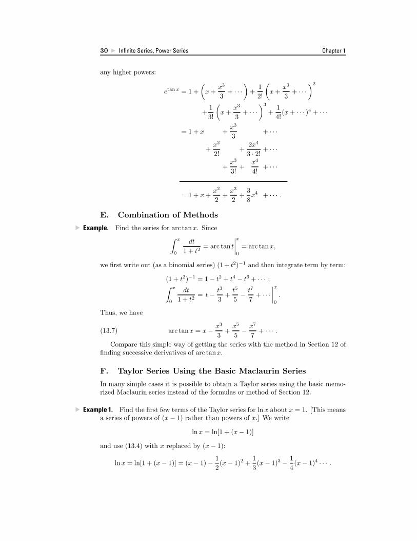
30 Infinite Series, Power Series Chapter 1
any higher powers:
etan x = 1 +(
x +x3
3+ · · ·
)+
12!
(x +
x3
3+ · · ·
)2
+13!
(x +
x3
3+ · · ·
)3
+14!
(x + · · · )4 + · · ·
= 1 + x +x3
3+ · · ·
+x2
2!+
2x4
3 · 2!+ · · ·
+x3
3!+
x4
4!+ · · ·
= 1 + x +x2
2+
x3
2+
38x4 + · · · .
E. Combination of Methods
Example. Find the series for arc tanx. Since∫ x
0
dt
1 + t2= arc tan t
∣∣∣∣x
0
= arc tanx,
we first write out (as a binomial series) (1+ t2)−1 and then integrate term by term:
(1 + t2)−1 = 1 − t2 + t4 − t6 + · · · ;∫ x
0
dt
1 + t2= t − t3
3+
t5
5− t7
7+ · · ·
∣∣∣∣x
0
.
Thus, we have
(13.7) arc tanx = x − x3
3+
x5
5− x7
7+ · · · .
Compare this simple way of getting the series with the method in Section 12 offinding successive derivatives of arc tanx.
F. Taylor Series Using the Basic Maclaurin Series
In many simple cases it is possible to obtain a Taylor series using the basic memo-rized Maclaurin series instead of the formulas or method of Section 12.
Example 1. Find the first few terms of the Taylor series for ln x about x = 1. [This meansa series of powers of (x − 1) rather than powers of x.] We write
ln x = ln[1 + (x − 1)]
and use (13.4) with x replaced by (x − 1):
ln x = ln[1 + (x − 1)] = (x − 1) − 12(x − 1)2 +
13(x − 1)3 − 1
4(x − 1)4 · · · .

Section 13 Techniques for Obtaining Power Series Expansions 31
Example 2. Expand cosx about x = 3π/2. We write
cosx = cos[3π
2+
(x − 3π
2
)]= sin
(x − 3π
2
)
=(
x − 3π
2
)− 1
3!
(x − 3π
2
)3
+15!
(x − 3π
2
)5
· · ·
using (13.1) with x replaced by (x − 3π/2).
G. Using a Computer
You can also do problems like these using a computer. This is a good methodfor complicated functions where it saves you a lot of algebra. However, you’re notsaving time if it takes longer to type a problem into the computer than to do itin your head! For example, you should be able to just write down the first fewterms of (sin x)/x or (1 − cosx)/x2. A good method of study is to practice doingproblems by hand and also check your results using the computer. This will turnup errors you are making by hand, and also let you discover what the computerwill do and what it won’t do! It is very illuminating to computer plot the functionyou are expanding, along with several partial sums of the series, in order to see howaccurately the partial sums represent the function—see the following example.
–2 –1.5 –1 –0.5–0.5
0.5
11.5
2
2.5
–1
0.5 1 1.5
S1
–2 –1.5 –1 –0.5
–0.5
0.5
1
1.5
0.5 1 1.5
S3
–2 –1.5 –1 –0.5
–0.5
0.5
1
1.5
0.5 1 1.5
S5
–2 –1 –0.5
–0.5
–1
0.5
1
1.5
0.5 1 1.5
S4
–1.5
Figure 13.1
Example. Plot the function ex cosx together with several partial sums of its Maclaurinseries. Using Example 2 in 13A or a computer, we have
ex cosx = 1 + x − x3
3− x4
6− x5
30· · · .
Figure 13.1 shows plots of the function along with each of the partial sums S1 = 1+x,S3 = 1 + x − x3
3 , S4 = 1 + x − x3
3 − x4
6 , S5 = 1 + x − x3
3 − x4
6 − x5
30 . We can seefrom the graphs the values of x for which an approximation is fairly good. Also seeSection 14.


