International Journal on Electrical Engineering and Informatics ‐ Volume 7, Number 1, March 2015 Mathematical modeling and analysis of a Generalized Unified Power Flow Controller with Device rating Methodology Chintalapudi Venkata Suresh and Sirigiri Sivanaga Raju Department of Electrical & Electronics Engineering, UCEK, JNTU Kakinada, Kakinada, A.P., India, 533 003. [email protected] and [email protected]Abstract: Ever incrasing demand on power system needs latest FACTS devices to increase the power transfer capability. One of such device is Generalized Unified Power Flow Controller. This device has got more emphasis, as it has five/more degree of freedom, it can simultaneously control the voltage at the sending end and the power flow through the transmission lines to which the device is connected. The detailed Power Injection Model (PIM) of GUPFC is proposed in this paper. Location and rating of the device plays a major role, to get proper control in power system. An optimal placement strategy based on single line contingencies through performance index is proposed. Without loss of generality, device rating is calculated based on the power handling capacity of the converters. Series and Shunt Converter switching losses and the shunt converter reactive power injection are considered, to analyze the effect of the device. Analytical results confirms the effect of the device control parameters on a given test system. Keywords: Generalized Unified Power Flow Controller, Power Injection Model, Performance Index, Contingency Analysis, FACTS device rating. 1. Introduction Flexible AC Transmission Systems (FACTS) has got good reputation because of getting higher controllability and increasing power transfer capability by means of power electronic based converters [1]. Basically these devices reduce the network expansion cost/transmission lines installation cost, by properly managing the system parameters. The basic applications of the FACTS devices are: power flow control, increase of transmission capability, voltage control, reactive power compensation, stability improvement, power quality improvement, etc [2]. It can be seen that with the growing demand for electricity, the opportunity for FACTS-devices gets more and more important. The Unified Power Flow Controller (UPFC) can be used for simultaneous control of the power system parameters (voltage, impedance, phase angle), or any of the above combinations [3, 4]. A comprehensive load flow model for UPFC, to incorporate into existing Newton-Raphson (NR) Load flow is presented in [5]. An algorithm is proposed for determining the optimum flow and size of UPFC for power flow applications [6]. The UPFC operation, control, sequencing, and protection methodologies under practical constraints are discussed in [7]. An effective modeling of UPFC and its performance has been presented in [8, 9]. A set of analytical equations are derived to control any combination of the power system parameters or none of them [10]. It is possible to study the power flow control in the presence of UPFC by obtaining sensitivity matrix of the power system[11]. The congestion management in power system is possible with the selection of suitable location and settings of its control parameters[12]. An effective injection modeling approaches to power flow analysis in the presence of UPFC is discussed in [13-15]. Power Injection Model (PIM) of UPFC and its effect, based on location are analyzed in [16, 17]. Advanced UPFC model to reuse NR Load flow has been developed in [18]. It is possible to extend the concept of voltage and power flow control beyond what is achievable with the UPFC; name of the device is Generalized Unified Power Flow Controller (GUPFC). Figure 1 shows the principle configuration of the GUPFC. Simply, it consists of Received: September 9 th , 2014. Accepted: March 7 th , 2015 DOI: 10.15676/ijeei.2015.7.1.5 59
Transcript
International Journal on Electrical Engineering and Informatics ‐ Volume 7, Number 1, March 2015
Mathematical modeling and analysis of a Generalized Unified Power Flow Controller with Device rating Methodology
Chintalapudi Venkata Suresh and Sirigiri Sivanaga Raju
Department of Electrical & Electronics Engineering, UCEK, JNTU Kakinada,
Abstract: Ever incrasing demand on power system needs latest FACTS devices to increase the power transfer capability. One of such device is Generalized Unified Power Flow Controller. This device has got more emphasis, as it has five/more degree of freedom, it can simultaneously control the voltage at the sending end and the power flow through the transmission lines to which the device is connected. The detailed Power Injection Model (PIM) of GUPFC is proposed in this paper. Location and rating of the device plays a major role, to get proper control in power system. An optimal placement strategy based on single line contingencies through performance index is proposed. Without loss of generality, device rating is calculated based on the power handling capacity of the converters. Series and Shunt Converter switching losses and the shunt converter reactive power injection are considered, to analyze the effect of the device. Analytical results confirms the effect of the device control parameters on a given test system. Keywords: Generalized Unified Power Flow Controller, Power Injection Model, Performance Index, Contingency Analysis, FACTS device rating. 1. Introduction Flexible AC Transmission Systems (FACTS) has got good reputation because of getting higher controllability and increasing power transfer capability by means of power electronic based converters [1]. Basically these devices reduce the network expansion cost/transmission lines installation cost, by properly managing the system parameters. The basic applications of the FACTS devices are: power flow control, increase of transmission capability, voltage control, reactive power compensation, stability improvement, power quality improvement, etc [2]. It can be seen that with the growing demand for electricity, the opportunity for FACTS-devices gets more and more important. The Unified Power Flow Controller (UPFC) can be used for simultaneous control of the power system parameters (voltage, impedance, phase angle), or any of the above combinations [3, 4]. A comprehensive load flow model for UPFC, to incorporate into existing Newton-Raphson (NR) Load flow is presented in [5]. An algorithm is proposed for determining the optimum flow and size of UPFC for power flow applications [6]. The UPFC operation, control, sequencing, and protection methodologies under practical constraints are discussed in [7]. An effective modeling of UPFC and its performance has been presented in [8, 9]. A set of analytical equations are derived to control any combination of the power system parameters or none of them [10]. It is possible to study the power flow control in the presence of UPFC by obtaining sensitivity matrix of the power system[11]. The congestion management in power system is possible with the selection of suitable location and settings of its control parameters[12]. An effective injection modeling approaches to power flow analysis in the presence of UPFC is discussed in [13-15]. Power Injection Model (PIM) of UPFC and its effect, based on location are analyzed in [16, 17]. Advanced UPFC model to reuse NR Load flow has been developed in [18]. It is possible to extend the concept of voltage and power flow control beyond what is achievable with the UPFC; name of the device is Generalized Unified Power Flow Controller (GUPFC). Figure 1 shows the principle configuration of the GUPFC. Simply, it consists of Received: September 9th, 2014. Accepted: March 7th, 2015 DOI: 10.15676/ijeei.2015.7.1.5
59
three converters, one connected in shunt and the other two are in series with two transmission lines at a bus. This basic configuration can control total five power system quantities such as a bus voltage and independent active and reactive power flow in two lines.
Figure 1. Principle configuration of GUPFC
The complete working procedure and fundamental frequency model of GUPFC is described in [19]. In [20], a mathematical model of the GUPFC suitable for power flow is proposed. Voltage source based mathematical models of the GUPFC and its implementation in Newton power flow is presented in [21]. In [22], the application of GUPFC in a real power grid for power flow as well as voltage control by applying a four converter GUPFC in Sichuan power system of China is analyzed. Steady state mathematical model of GUPFC, based on d-q axis reference frame decomposition has been derived in [23]. Robust modeling of the GUPFC with small impedances in power flow analysis is given in [24]. A fuzzy rule based model for GUPFC is proposed in [25]. Nonlinear predictor-corrector primal-dual interior-point optimal power flow algorithm for GUPFC is presented in [26]. The design of the GUPFC damping controller is designed in [27]. Analysis of sub synchronous resonance with GUPFC is presented in [28]. The concept of GUPFC can be extended for more lines, if necessary. By using GUPFC devices, the transfer capability of transmission lines can be increased significantly. Further mores, by using the multi-line management capability of GUPFC; active power flows on lines can not only be increased, but also be decreased with respect to operating and market transaction requirement [24]. From the careful review of the literature, it is identified that, in the GUPFC modeling, the switching converter losses are not considered. In this paper, the main contribution is to develop Power Injection Model (PIM) of GUPFC with converter switching losses to get an effective control and secured operation. A proper location to install the device is calculated by using single line contingency analysis. An optimal rating of the device is estimated without loss of generality i.e. by using power handling capability of the device subjected to the system loading conditions. The main advantage of the proposed methodology is that, the rating and the optimal location of GUPFC are obtained to show the effectiveness of the device on system parameters, which is not available in the existing literature. The efficiency of the proposed model is tested on Hale Network. A. Critic on Literature Most of the literature has not given the detailed mathematical PIM of GUPFC in an optimal location with proper size to analyze the effect of the same on a given power system. So, there is a need of such a stated modeling to get proper control over the network to optimize certain objectives. Hence in this paper, optimal location finding strategy, proper device size calculation strategy, and a detailed analysis of the GUPFC power injection model are presented.
Chintalapudi Venkata Suresh, et al.
60
2. Operating principle of GUPFC There are several possibilities of operating configurations by combining two or more converter blocks with flexibility. The GUPFC with combining three or more three-phase switching converters connected back-back through coupling transformers. The main function of the converter is to change a DC input voltage to a symmetrical AC output voltage of desired magnitude, frequency and phase shift with respect to the selected reference. The function of coupling transformers is to isolate GUPFC and transmission line and to match the voltage levels between the line and the voltage produced by the converters. Series converter inserts voltage of controllable magnitude and controllable phase angle in series with the transmission line via series connected transformer, thereby it provides the control of real and reactive power flow in the transmission line. The real power injected into the system by the series branches must be taken from the parallel branch through dc link. The real power flows in either direction between AC terminals of the converters. 3. GUPFC Mathematical modeling A GUPFC can be represented by three voltage sources, which are controllable in both magnitude and phase angle and are representing fundamental components of output voltages of three converters & impedances being leakage reactance’s of three coupling transformers. Let us define three GUPFC buses i, j and k as shown in Figure 2. The following considerations are taken for analysis purpose: 1. Voltage at bus-i is taken as iii VV δ∠= 2. The two controllable series injected voltage sources are identical. 3. The leakage reactance of the two series coupling transformers is equal. The two controllable series voltage sources source 1seV and 2seV are defined as
γj
isesese erVVVV === 21 (1) where ‘r’ and ‘γ ’ are respective per unit magnitude and phase angles of series voltages, and which are operating in the following specified limits
maxrr ≤≤0 and maxγγ ≤≤0 The GUPFC device is incorporated in between three GUPFC buses, out of which one is a common bus for the remaining two buses. Briefly, one of the series converters is connected between bus-i and bus-j, similarly, another series converter is connected between bus-i and bus-k. The GUPFC power injection model is developed in two stages, one is series connected voltage source model and the other is shunt connected voltage source model. The voltages behind the series reactance’s can be calculated as
2'
1' = = seiikseiij VVVandVVV ++
(2)
Figure 2. Voltage source model of GUPFC
Mathematical modeling and analysis of a Generalized Unified Power Flow
61
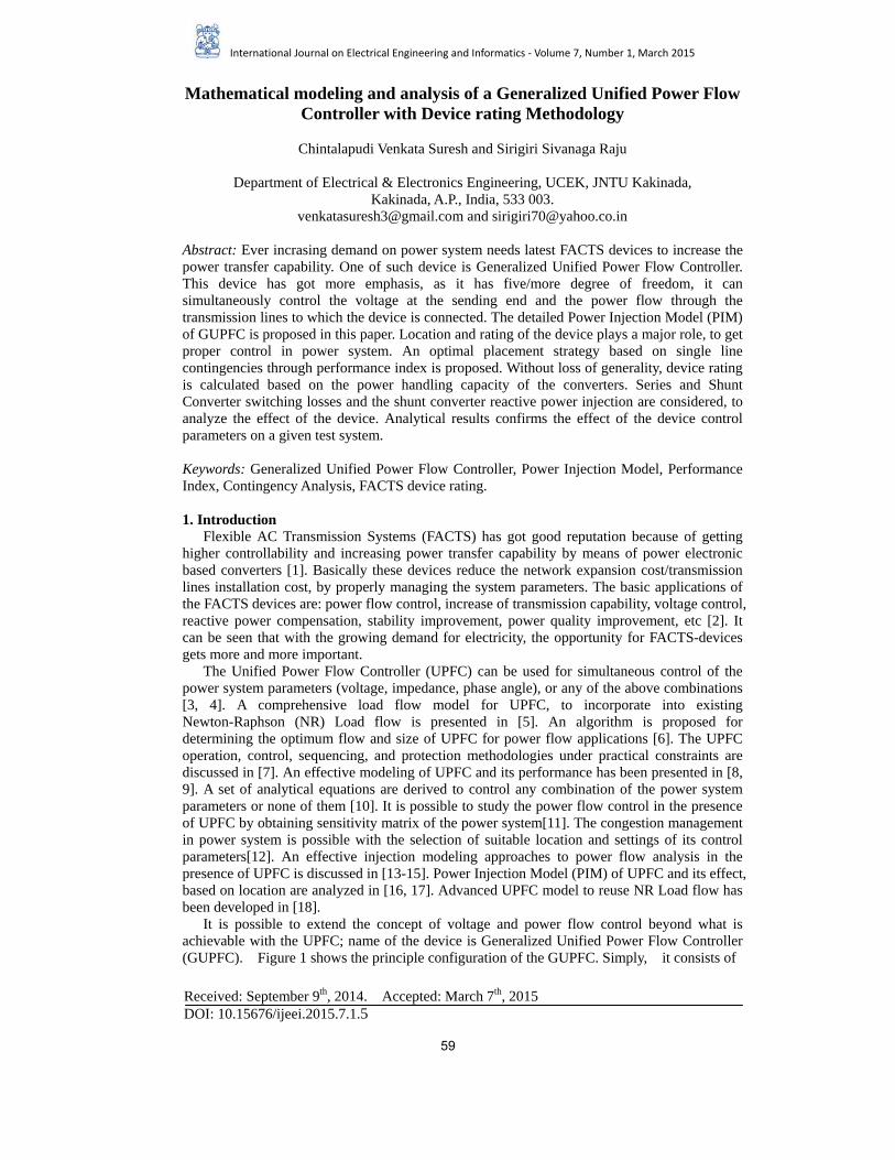
Figure 3. Equivalent current source model of GUPFC
A. Series connected voltage source mode According to Norton’s theorem, the series connected voltage source can be modeled by replacing the voltage source ‘ seV ’ with an equivalent current source ‘ seI ’ in parallel with a transmission line susceptance ‘ seB ’ as shown in figure 3. where
sese X
B 1= (3)
seX is the series transformer equivalent reactance The amount of current flowing from the source is given as
sesese
sese VjB
jXVI −== (4)
replace seV in Eq.(4) from Eq.(1)
)(90)(
==γδγδ +++
−− ijsei
ijseise eBrVeBjrVI
o
(5)
hence
)(90* =)(
γδ ++−− ij
seise eBrVIo
(6) This current source can be modeled by injecting equivalent powers at the respective buses, to which the device is connected. The corresponding power injections are shown in figure.4. This model can be seen as the three independent complex powers injections at the GUPFC buses and can be written as
*)(2= seisei IVS −
(7)
*)(= sejsej IVS
(8)
*)(= seksek IVS
(9)
the detailed expressions for these injections can be deduced by substituting Eq. (6) in Eqs. (7)-(9)
)(9022= γ+− oj
seisei eBrVS
Chintalapudi Venkata Suresh, et al.
62
)(90
=γδδ +−+−
− jijsejisej eBVrVS
o
)(90
=γδδ +−+−
− kijsekisek eBVrVS
o
by using Eulers identity, ααα sincos je j += ; let us define jiij δδδ −= and kiik δδδ −=
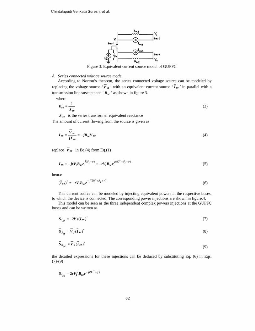
by using trigonometric identities in Eqs (10)-(12), the active and reactive power injections at i, j, k are
)(2= 2 γsinseisei BrVP −
(13)
)(2= 2 γcosseisei BrVQ −
(14)
)(= γδ +ijsejisej BVrVP sin
(15)
)(= γδ +ijsejisej BVrVQ cos
(16)
)(= γδ +iksekisek BVrVP sin
(17)
)(= γδ +iksekisek BVrVQ cos
(18)
The equivalent series connected voltage source model with the corresponding power injections
is shown in figure 4.
Figure 4. Equivalent series connected voltage source model
Mathematical modeling and analysis of a Generalized Unified Power Flow
63
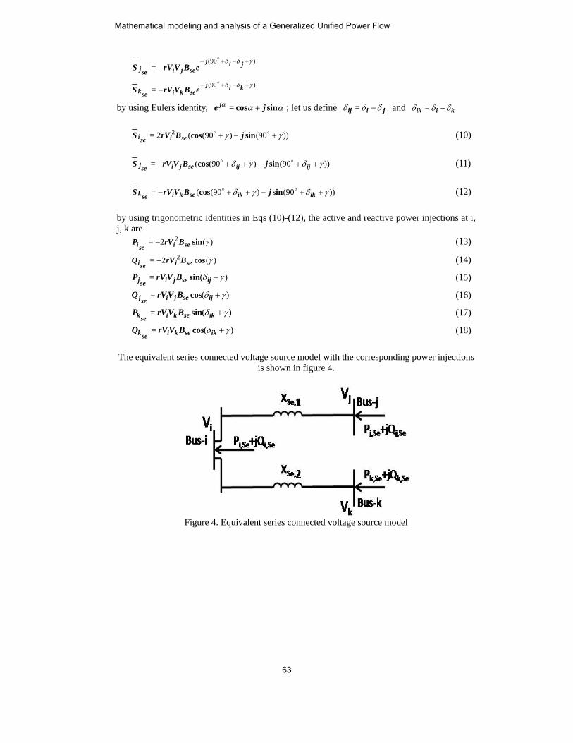
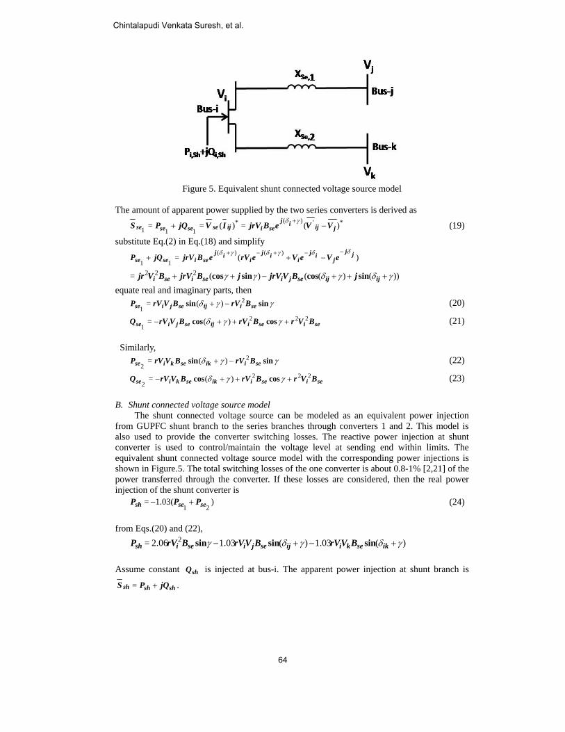
Figure 5. Equivalent shunt connected voltage source model
The amount of apparent power supplied by the two series converters is derived as
*')(*111 )(=)(== jijij
seiijsesesese VVeBjrVIVjQPS −++γδ
(19)
substitute Eq.(2) in Eq.(18) and simplify
)(=)()(
11jj
jij
iij
iij
seisese eVeVerVeBjrVjQPδδγδγδ −−+−+
−++
))()(()(= 222 γδγδγγ +++−++ ijijsejiseisei jBVjrVjBjrVBVjr sincossincos equate real and imaginary parts, then γγδ sinsin seiijsejise BrVBVrVP 2
1)(= −+
(20)
seiseiijsejise BVrBrVBVrVQ 2221
)(= +++− γγδ coscos
(21)
Similarly, γγδ sinsin seiiksekise BrVBVrVP 2
2)(= −+
(22)
seiseiiksekise BVrBrVBVrVQ 2222
)(= +++− γγδ coscos
(23)
B. Shunt connected voltage source model The shunt connected voltage source can be modeled as an equivalent power injection from GUPFC shunt branch to the series branches through converters 1 and 2. This model is also used to provide the converter switching losses. The reactive power injection at shunt converter is used to control/maintain the voltage level at sending end within limits. The equivalent shunt connected voltage source model with the corresponding power injections is shown in Figure.5. The total switching losses of the one converter is about 0.8-1% [2,21] of the power transferred through the converter. If these losses are considered, then the real power injection of the shunt converter is
Assume constant shQ is injected at bus-i. The apparent power injection at shunt branch is
shshsh jQPS += .
Chintalapudi Venkata Suresh, et al.
64
C. GUPFC mathematical model The final steady state model of GUPFC power injection model is obtained by combining series connected voltage and shunt connected voltage source models. Then the equivalent GUPFC model is shown in Figure 6. The resultant power injections are given as
D. Computational flow Initially contingency analysis is performed for a given system to find a place where two lines attached to the critical bus, to install GUPFC. After this the device rating is calculated by using the procedure mentioned in the section 5 and using the flow chart shown in Figure.7. Then, the complete analysis of the effect of GUPFC on a given test system is performed by using NR load flow. To study the impact of GUPFC on an electrical power network, the device model should be incorporated into the system. Power Injection Model is a popularly used model to incorporate the device by changing the Jacobian and power mismatche equations in Newton-Raphson algorithm[16]. The linearized system model based on NR algorithm is written as,
nnn
VV
LJNH
QP
⎥⎥⎦
⎤
⎢⎢⎣
⎡ΔΔ
⎥⎦
⎤⎢⎣
⎡⎥⎦
⎤⎢⎣
⎡ΔΔ δ
=
(31)
The algorithm for solving power flow problem embedded with “UPFC" is implemented for “GUPFC"[16]. The corresponding power mismatches Eqs.(34) to (39) and corresponding Jacobian elements are given in Eqs.(40) to (67).
Mathematical modeling and analysis of a Generalized Unified Power Flow
65
4. Optimal location Contingency analysis is a procedure of removing an alternator, transformer, or a transmission line for temporarily or permanently based on the requirement. Because of this the system may enter into an unstable state which may be insecure. This analysis got very importance in power system analysis to predict the contingencies so that the preventive/corrective actions can be taken appropriately. In this paper, single transmission line contingency approach is followed [29]. For each line outage, the total lines which violate the maximum power flow (OLL) and the total buses which violate the minimum/maximum voltage limits (VVB) are identified. The performance index (PI) is calculated by performing the summation of the total number of over loaded lines (NOLL) and total number of voltage violated buses (NVVB). i.e PI = NOLL + NVVB. Rank is allotted to the contingencies based on the performance index[30]. The line with highest performance index is the most severe than the remaining. Then, the shunt converter is placed at the critical bus and the two series converters are placed in the transmission lines which are connected to the critical bus and is based on the line reactance and also the line flow limits. The contingency ranking of the test system is given in Table.1. 5. Device size calculation To get an effective and required control action, estimating proper size of GUPFC plays an important role in the present day power system FACTS device installation . Without violating loss of generality, the device power rating should be more than the device operating power in a system.
Figure 7. Flow chart to calculate device rating
Chintalapudi Venkata Suresh, et al.
66
Based on this principal the device rating is calculated as follows: The reactance seen from the terminals of the series converter transformer (in p.u base on system voltage and base power) can be calculated as [6]
S
BmaxkS
SSrxX 2=
(32)
where kx is the series transformer reactance, ‘ maxr ’ is the factor to maximum p.u value of the
injected voltage magnitude, ‘ BS ’ is the system base power, and ‘ SS ’ is the nominal power rating of the series converter. Normally in transmission system, frequently used power transformers specifications are in, MVA, kV, %Z, Hz. By using these specifications, the transformer reactance ( kx ) can be calculated from the fundamentals as
Ω××
100% )(=
2
MVAZkVxk
(33)
Figure 7 shows the flow chart to determine the device rating. 6. Numerical results A. Setting of the proposed approach A MATLAB code has been developed to perform contingency analysis for finding the device location, to determine the device rating and also to analyze the effect of GUPFC on a given power system on a computer with 2.5 GHz processor and with 2GB RAM. The capability/compactness of the code can be calibrated in terms of the execution time. The time taken for each iteration with constant ‘r’ and ‘ γ ’ varies from 00 to 3600 with 100 interval is around 15-20 sec. In this study, the standard Hale Network is considered to investigate the effectiveness of the proposed strategy. The data is taken from [31]. B. Illustration of contingency analysis
The single line contingency analysis procedure is performed on the test system for determining the proper location and results are tabulated in Table 1. From this, it is observed that bus-5 is the critical one and the lines connected to this bus are ‘line-6’ and ‘line-7’. Hence the device is placed in this location.
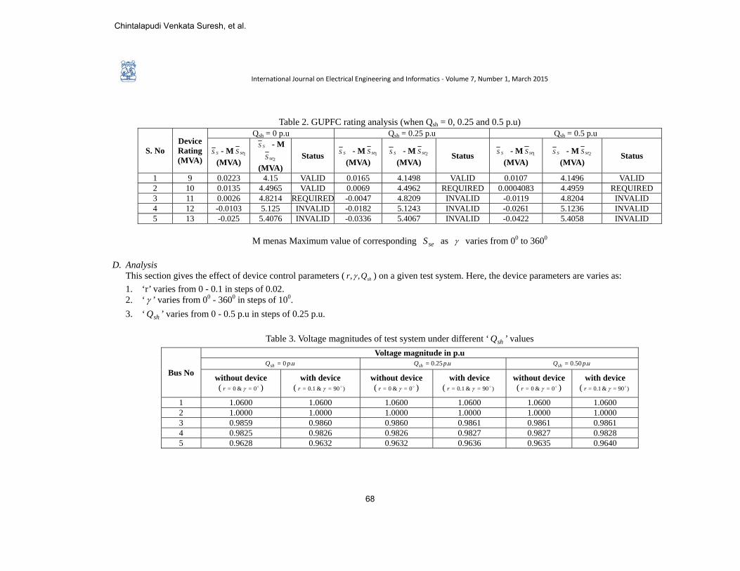
C. Optimal device rating Based on the procedure mentioned in section 5, the device rating of the test system is calculated and are tabulated in Tables.2 with different ‘ shQ ’ values. To show the validity of the methodology, power transfoermer specifications considered in this paper are 100MVA, 138 kV, 12.7 %Z, 50 Hz. From these results, it is observed that the required nominal power rating of the converter is 10MVA.
Mathematical modeling and analysis of a Generalized Unified Power Flow
67
International Journal on Electrical Engineering and Informatics ‐ Volume 7, Number 1, March 2015
Mathematical modeling and analysis of a Generalized Unified Power Flow
69
To illudevice cangives the voltage apoint herebus-5 is in The cofrom thesthe lines i The cobserved some of tis increas The acreactive pdecreased
Tab
Description
Total active power
loss (MW) Total reactive
power loss (MVAr)
Figur
ustrate the effn increase/decreffect of GU
at buses variese is that, voltancreases drastiorresponding pse tables is thatis increased/deorresponding pfrom these tab
the lines is incred. ctive and react
power losses ind drastically as
ble 6. Active anQsh
Without device
( o0=&0= γr )
6.2414
-7.7799
re 8. Voltage m
fect of device rease the magn
UPFC, on volta, as ‘r’ varies
age at load busically when Qpower flows in t, at constant Q
ecreased. power flows in
bles is that, at creased/decreas
tive power lossn the system ar
shQ is increas
nd reactive powup.0=
With device ( )90=&0.1= oγr
6.2390
-8.3637
magnitude and p
on the systemnitude of the voage magnitude
from 0-0.1 anses is increased
shQ increases frthe transmissi
shQ , the active
n the transmisconstant shQ , ted. But, these
ses are given ie decreased aftsed.
wer loss in theQsh
Without device( o0=&0= γr )
6.2387
-7.7960
phase angle va(at shQ =0
m, ‘r’=0.1 and oltages and ang of the buses.nd ‘γ ’ varies d after the devfrom 0-0.5 p.u aion lines is give
and reactive p
ssion lines is gthe active and rflows in many
n Table.6. At cfter GUPFC is p
system under up.0.25=
e)
With device( 90=&0.1= γr
6.2353
-8.3795
ariations at load0)
‘γ ’=900 is cogles at the buse This table refrom 00-200. T
vice is placed. at bus-5.en in Tables.4 power flows th
given in Tablesreactive powery lines gets dec
constant shQ , placed. But, th
different ‘ shQQsh
e )0 o
Without device
( o0=&0= γr
6.2360
-7.8119
d buses with ‘r
onsidered. Thees. The Table.3eveals that, theThe noticeableThe voltage at
. It is observed
hrough some of
s.4 and 5. It isr flows throughcreased as shQ
the active andhese losses gets
’ values uph .0.50=
)
With device ( 90=&0.1= γr
6.2327
-8.3951
’ variation
e 3 e e t
d f
s h
d s
)o
Chintalapudi Venkata Suresh, et al.
70
Figure‘γ ’ varieit is obser Figure7 as ‘γ ’ vthis it is c
Figu
Figure
e 8 shows the es from 00 to 36rved that there e 9 shows the vvaries from 00
clear that, activ
ure 9. Active an
10. Voltage ma
variation of vo600 and ‘ r ’ vais an increase variation of acto 3600 and ‘ r
ve power flow i
nd reactive pow
agnitude and p
oltage magnituaries from ‘0’ tin bus voltagestive and reactir ’ varies fromis increased in
wer flow variat(at shQ =0
phase angle var(at r=0.1)
udes and angleto ‘0.1’ with Qs as ‘γ ’ variesve power flow
m ‘0’ to ‘0.1’ wiall lines as ‘γ
tions in lines 10)
riations at load)
es at load buseshQ is equal to
s from 00 to 90ws through the ith shQ is equγ ’ varies from 3
,3,5,7 with ‘r’
d buses with Q
es 3,4 and 5 aso ‘0’. From this
0. lines 1,5,6 and
ual to ‘0’. From3000 to 3600.
variation
shQ variation
s s
d m
Mathematical modeling and analysis of a Generalized Unified Power Flow
71
Figure‘γ ’ varieshows, th Figure7 as ‘γ ’ This show
Figure
Figurevaries froit is clear from 400
Figur
e 10 shows thees from 00 to 36he bus voltage me.11 shows the varies from 00
ws, the active p
e 11. Active an
e 12 shows thom 00 to 3600 a
that, active poto 1600.
re 12. Active a
e variation of v600 and shQ vmagnitude incrvariation of ac
0 to 3600 and Q
power flow in l
nd reactive pow
he variation of and shQ variesower and reacti
and reactive po
voltage magnitvaries from ‘0’ reases as ‘ shQ ’ctive and reacti
shQ varies fromline-5 increased
wer flow variati(at r=0.1)
f active and res from ‘0’ to ‘0ive power losse
wer loss variat(at r=0.1)
tudes and anglto ‘0.5’p.u wi varies from 0 ive power flowm ‘0’ to ‘0.5’pd as ‘ shQ ’ vari
ions in lines 1,)
active power 0.5’p.u with ‘ res are decrease
tions in the sys)
es at load buseith ‘ r ’ is equato 0.05 p.u.
ws through the .u with ‘ r ’ is ies from 0 to 0
,3,5,7 with shQ
losses of test r ’ is equal to ‘0ed in the system
stem with shQ
es 3,4 and 5 asal to ‘0.1’. This
lines 1,5,6 andequal to ‘0.1’
0.05 p.u.
h variation
system as ‘ γ0.1’. From thism as ‘ γ ’ varies
variation
s s
d .
’ s s
Chintalapudi Venkata Suresh, et al.
72
Figureas ‘γ ’ vathe variat‘γ ’ is fixclear thatfrom 00 toin the sys
(a) and
(a) and (a
es 13(a) and (baries from 00 toion of active a
xed at 00 , 900 t, both active ao 1600. From Ftem gets decre
d (b) with ‘r’ vaFigure 13
b) with ‘ γ ’ vaand (d) is the d
Figure
b) shows, the vo 3600 and ‘ rnd reactive pow, 1800 , 2700 and reactive p
Figures. (c) andeased as ‘γ ’ is
ariation (c) and3. Active and r
aries from 00 todifference of co 14. Apparent p
variation of acti’ varies from ‘0wer losses in thwith shQ is e
power losses ind (d), it is clear maintained at
d (d) with ‘γ ’ eactive power
3600 and ‘ r ’ onverter apparepower variatio
ive and reactiv0’ to ‘0.1’ and he system as ‘requal to ‘0’. Frn the system gr that, both acti900.
fixed at 00, 90loss variations
varies from ‘0ent powers from
ons of the series
ve power lossesFigures.13(c) r’ varies from rom Figures. (agets decreased ive and reactiv
00, 1800 , 2700s in the system
0’ to ‘0.1’ with m the device ras converters
s in the systemand (d) shows,‘0’ to ‘0.1’ anda) and (b), it isas ‘γ ’ varies
ve power losses
0 (at shQ =0)
shQ =‘0’. (c)
ating.
m ,
d s s s
Mathematical modeling and analysis of a Generalized Unified Power Flow
73
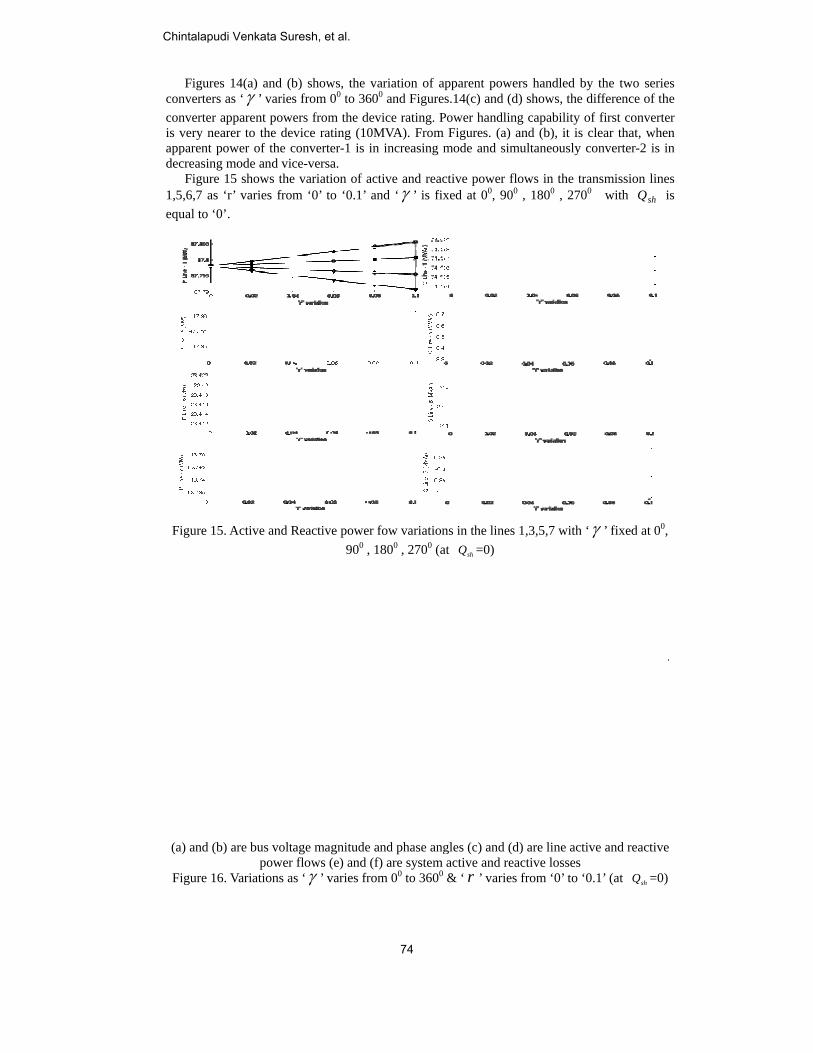
Figureconverterconverteris very neapparent decreasin Figure1,5,6,7 asequal to ‘
Figure 1
(a) and (
Figure 1
es 14(a) and (brs as ‘γ ’ varier apparent powearer to the depower of the cg mode and vie 15 shows thes ‘r’ varies fro0’.
5. Active and R
b) are bus voltpower
6. Variations a
b) shows, the s from 00 to 36
wers from the device rating (10converter-1 is ce-versa. e variation of am ‘0’ to ‘0.1’
Reactive powe900 ,
tage magnituder flows (e) and as ‘γ ’ varies fr
variation of a600 and Figuredevice rating. P0MVA). From in increasing m
active and reacand ‘γ ’ is fix
er fow variation, 1800 , 2700 (a
e and phase ang(f) are system
rom 00 to 3600
apparent powers.14(c) and (d)
Power handlingFigures. (a) a
mode and simu
ctive power floxed at 00, 900
ns in the lines 1at shQ =0)
gles (c) and (d)active and rea& ‘ r ’ varies
rs handled by ) shows, the dig capability of and (b), it is clultaneously co
ows in the tran, 1800 , 2700
1,3,5,7 with ‘γ
) are line activective losses from ‘0’ to ‘0.
the two seriesifference of thef first converterlear that, whenonverter-2 is in
nsmission lines with shQ is
γ ’ fixed at 00,
e and reactive
1’ (at shQ =0)
s e r n n
s s
Chintalapudi Venkata Suresh, et al.
74
Figure 16(a) and (b) shows the variation of the voltage magnitudes and phase angles at buses, (c) and (d) shows the active and reactive power flows in the transmission lines, (e) and (f) are active and reactive power losses in the transmission lines as ‘γ ’ varies from 00 to 3600 and ‘ r ’ varies from ‘0’ to ‘0.1’ with shQ is equal to ‘0’. 7. Conclusion The effect of multi-line controller (GUPFC) has been analyzed by using the proposed Power Injection Model of the device. Since it is the combination of the multiple converters, it can simultaneously control the voltage by using shunt converter and power flows (both active and reactive) through the transmission lines using series converters. All these converters are coordinated together to perform the device operation successfully. The proposed strategies, to find optimal location and device rating works in a constrictive manner to analyze the effect of device on a given test systems. The analytical resutls shows the variation of the system parameters like, bus voltage magnitudes and phase angles, line power flows and losses greatly effects based on the device parameters like ‘r’, ‘γ ’ and ‘ shQ ’. Finally, the developed PIM of the GUPFC can effectively controls the power system parameters of the test systems. 8. Appendices A. Modifications in Jacobian elements The modified diagonal and off-diagonal elements of ‘H’ are
gupfckgupfcj
i
gupfciii QQ
PH ,,
,' 1.031.03== −−∂
∂
θ (34)
gupfcj
j
gupfci
ij QP
H ,
,' 1.03==θ∂
∂ (35)
gupfck
k
gupfciik Q
PH ,
,' 1.03==θ∂
∂ (36)
gupfcj
j
gupfcjjj Q
PH ,
,' == −∂
∂
θ (37)
gupfcj
i
gupfcjji Q
PH ,
,' ==θ∂
∂ (38)
gupfck
k
gupfckkk Q
PH ,
,' == −∂
∂
θ (39)
gupfck
i
gupfckki Q
PH ,
,' ==θ∂
∂ (40)
Simillar modification can be applied for other Jacobian elements. B. Modifications in power mismatch equations The modifications in active and reactive power mismatches are given as (superscript ‘0’ indicates the power mismatches without device)
gupfciii PPP ,0= +ΔΔ (41)
gupfcjjj PPP ,
0= +ΔΔ (42)
Mathematical modeling and analysis of a Generalized Unified Power Flow
75
gupfckkk PPP ,
0= +ΔΔ (43)
gupfciii QQQ ,
0= +ΔΔ (44)
gupfcjjj QQQ ,
0= +ΔΔ (45)
gupfckkk QQQ ,
0= +ΔΔ (46)
9. System Data The single line diagram with corresponding data of the Hale Netwrok is shown in Figure.17.
Figure 17. Hale Network
10. References [1] N.G. Hingorani.,“Flexible AC transmission", IEEE Spectrum 30,1993,pp. 40-45. [2] Xiao-Ping Zhang, Christian Rehtanz, Bikash Pal.,“Flexible AC Transmission Systems:
Modelling and Control (Power Systems)",Springer (March 2006)., ISBN:3540306064. [3] L. Gyugyi.,“Unified power flow control concept for Flexible AC Transmission systems",
IEE Proceedings on Generation, Transmission and Distribution, 1992, Vol 139, No. 4, pp. 323-331.
[4] L Gyugyi, C D Schauder, et al.,“The Unified Power Flow Controller:A new appraoch to power transmission control", IEEE Transactions on Power Delivery, 1995, Vol. 10, No. 2, pp. 1085-1097.
[5] C R Fuerte Esquivel, E Acha.,“Unified power flow controller:a critical comparison of Newton-Raphson UPFC algorithms in power flow studies", IEE Proceedings on Generation, Transmission and Distribution, 1997, Vol 144, No. 5, pp. 437-444.
[6] M Noroozian, L Angquist, M Ghandhari, G Anderson.,“Use of UPFC for optimal power flow control", IEEE Transactions on Power Delivery, 1997, Vol. 12, No. 4, pp.1629-1634.
[7] C D Schauder, L Gyugyi, M R Lund, et al.,“Operation of the Unified Power Flow Controller (UPFC) under practical constraints", IEEE Transactions on Power Delivery, 1998, Vol 13, No. 2, pp. 630-639.
[8] A J F Keri, A S Mehraban., et al., “Unified Power Flow Controller(UPFC):Modeling and Analysis", IEEE Transactions on Power Delivery, 1999, Vol 14, No. 2, pp. 648-654.
[9] B A Renz, A Keri, et al.,“AEP Unified Power Flow Controller Performance", IEEE Transactions on Power Delivery, 1999, Vol. 14, No. 4, pp. 1374-1381.
Chintalapudi Venkata Suresh, et al.
76
[10] C R Fuerte Esquivel, E Acha, H Ambriz Perez.,“A Comprehensice Newton-Raphson UPFC Model for the Quadratic Power Flow Solution of Practical Power Networks", IEEE Transactions on power systems, 2000, Vol. 15, No. 1, pp. 102-109.
[11] Wanliang Fang, H W Ngan.,“A robust load flow technique for use in power system with unified power flow controller", Electric Power Systems Reseach., 2000, Vol 53, pp. 181-186.
[12] K S Verma, S N Singh, H O Gupta.,“Location of unified power flow controller for congestion management", Electrical Power and Energy Systems, 2001, Vol. 58, pp. 89-86.
[13] D Z Fang, Z Fang, H F Wang.,“Application of the injection modeling approach to power flow analysis for systems with unified power flow controller", Electrical Power and Energy Systems, 2001, Vol. 23, pp. 421-425.
[14] A. L Abbate, M. Trovato, C. Becker, E. Handschin.,“Advanced Steady-State Model of UPFC for Power System Studies", Power Engineering Society Summer Meeting (IEEE), 2002, Vol. 1, pp 449-454.
[15] M H Haque, C M Yam.,“A simple method of solving the controlled load flow problem of a power system in the presence of UPFC", Electric Power Systems Reseach., 2003, Vol 65, pp. 55-62.
[16] Mehmet Tumay, A M Vural, K L Lo.,“The effect of unified power flow controller location in power systems", Elecrical Power and Energy Systems, 2004, Vol. 26, pp. 561-569.
[17] A Mete Vural, Mehmet Tumay.,“Mathematical modeling and analysis of a unified power flow controller: A comparision of two appraoches in power flow studies and effects of UPFC location", Electrical Power and Energy Systems, 2007, Vol. 29, pp. 617-629.
[18] Suman Bhowmick, Biswarup Das, Narendra Kumar.,“An Indirect UPFC Model to Enhance Reusability of Newton Power Flow Codes", IEEE Transactions on Power Delivery, 2008, Vol. 23, No. 4, pp. 2079-2088.
[19] B. Fardanesh, B. Shperling, E. Uzunovic, S.Zelingher.,“Multi-Converter FACTS Devices:The Generalized Unified Power Flow Controller (GUPFC)", Power Engineering Society Summer Meeting, 2000. IEEE., Vol. 2, pp. 1020-1025.
[20] Xiao-Ping Zhang, Edmund Handschin, Maojun Mike Yao.,“Modeling of the Generalized Unified Power Flow Controller (GUPFC) in a Nonlinear Interior Point OPF", IEEE Transactions on Power Systems, Vol 16, No. 3, 2001, pp 367-373.
[21] X P Zhang.,“Modelling of the interline power flow controller and the generalised unified power flow controller in Newton power flow", IEE Proceedings on Generation, Transmission and Distribution, 2003, Vol 150, No. 3, pp. 268-274.
[22] Lin Sun Shengwei Mei, Qiang Lu, Jin Ma.,“Application of GUPFC in China’s Sichuan Power Grid-Modeling, Control Strategy and Case Study", Power Engineering Society General Meeting (IEEE), 2003, Vol. 1, pp. 175-181.
[23] Sheng-Huei Lee, Chia-Chi Chu.,“Power Flow Computations of Convertible Static Compensators for Large-Scale Power Systems", Power Engineering Society General Meeting (IEEE), 2004, Vol. 1, pp. 1172-1177.
[24] X P Zhang.,“Robust modeling of the interline power flow controller and the generalized unified power flow controller with small impedances in power flow analysis", Electrical Engineering (Springer Verlag), 2006, Vol.89, pp. 1-9.
[25] J G Singh, P Tripathy, S N Singh, C Srivastava.,“Development of a fuzzy rule based generalized unified power flow controller", European Transactions on Electrical Power, 2009, Vol.19, pp. 702-717.
[26] Rakhmad Syafutra Lubis, Sasongko Pramono Hadi, Tumiran.,“Modeling of the Generalized Unified Power Flow Controller for Optimal Power Flow", ICEEI (IEEE), 2011, pp. 1-6.
[27] Rakhmad Syafutra Lubis., “Modeling and Simulation of Generalized Unified Power Flow Controller (GUPFC)", 2nd International Conference on ICICI-BME (IEEE), 2011., pp. 207-213.
Mathematical modeling and analysis of a Generalized Unified Power Flow
77
[28] R ThresoSyst
[29] H I basePowEner
[30] Imanmod
[31] StagInc.,
Voltage S
hirumalaivasannance with genems, 2013, VolShaheen, G I R
ed in GA and Pwer and Energrgy in the 21st n Ziari, Alirez
dified PSO", Elgg N G, El-Abi, 1968.
Chinin thColleUniveAppliSysteContr
SirigElectKakinA.P., TechndoctoHydeElect
Stability, Power
n, Nagesh Prabneralized unifil.53, pp. 623-6Rashed, S J ChPSO for Enhancgy Society Gen
Century (IEEEza Jalilian.,“Oplectrical Poweriad H A.,“Com
talapudi Venkhe department ege of Enginersity Kakinadications in Pow
em Analysis incrol.
giri Sivanaga trical and Elecnada, Jawaharl
India. He conology, Khargporal program erabad, Andhratrical Distribur System Analy
bhu, M Janaki, ied power flow31.
heng.,“Optimalcing Power Syneral Meeting E), 2008, pp. 1ptimal placemer and Energy S
mputer Methods
kata Suresh (of Electrical
neering Kakida, Kakinada, Awer Systems, cluding FACTS
Raju (Non-mctronics Enginelal Nehru Tech
ompleted his Mpur, India, in e
from Jawaha Pradesh, Indiaution System ysis, and Powe
D P Kothari.,“w controller", E
l Location and ystem Security
- Conversion-8. ent and sizingSystems, 2012,s in Power Sys
(Non-member)and Electron
nada, JawahaA.P., India. HisOptimization S devices and P
member) is Proeering, Univerhnological UniMaster’s degrelectrical poweharlal Nehru a. His interests
Automation, er System Oper
“Analysis of suElectrical Pow
Parameters Seunder Single C
n and Delivery
of multiple AVol. 43, pp. 63
stem Analysis",
is currently pnics Engineerinarlal Nehru s interests incluTechniques, FPower System
ofessor in the rsity College oiversity Kakinaee from India
er systems. He Technologic
s include FACTOptimization
ration and Con
ubsynchronouswer and Energy
etting of UPFCContingencies"y of Electrical
APLCs using a30-639. , McGraw-Hill
pursuing Ph.Dng, UniversityTechnological
ude, ComputerFACTS, Power
Operation and
department ofof Engineeringada, Kakinada,an Institute ofcompleted hisal University