Abstract This paper deals with the mathematical mod-eling and algorithms for the problem of oil pollution.For solving this task, we derive the adjoint problem forthe advection–diffusion equation describing the prop-agation of oil slick after an accident, which we callthe main problem. We prove a fundamental equalitybetween the solutions of the main and the adjointproblems. Based on this equality, we propose a novelmethod for the identification of the pollution sourcelocation and the accident time of oil emission. Thisapproach is illustrated on an example for an accident inthe offshore of the central part of the Vietnamese coast.Numerical simulations demonstrate the effectiveness ofthe proposed method. Besides, the method is verifiedfor 1D model of substance propagation.
Q. A. DangInstitute of Information Technology,18 Hoang Quoc Viet, Ha noi, Vietname-mail: [email protected]
M. Ehrhardt (B)Lehrstuhl für Angewandte Mathematikund Numerische Analysis, Fachbereich C Mathematikund Naturwissenschaften, Bergische Universität Wuppertal,Gaußstrasse 20, 42119 Wuppertal, Germanye-mail: [email protected]
G. L. TranInstitute of Mathematics,18 Hoang Quoc Viet, Ha noi, Vietname-mail: [email protected]
D. LeBuro of Hydrology and Meteorology,Dang Thai Than, Ha noi, Vietname-mail: [email protected]
In this work, we study a mathematical model of oilspill processes in seas (arising from tanker or offshoreaccidents, liquid waste, etc.), such as advection, turbu-lent diffusion, surface spreading, evaporation, dissolu-tion, and emulsification. These processes may influencethe transport of oil spill. There exist a wide range ofresearch articles focused on the surface movement ofoil spills and describing the numerical simulation of oilspills in accidents occurred in some seas [28]. However,a large part of mathematical investigations of the usedcomputational schemes is still almost open. Therefore,the first goal of this paper is the analysis of numericalschemes for simulating oil spills in order to obtainaccurate predictions of the movement and the fate ofthe spilled oil. This forecast gives an idea of the oil spillimpact and is crucial for properly designed clean-uprecovery operations and the protection of ecologicallysensitive zones. After completing this task, we shallobtain good numerical schemes for predicting the oilslick at any time.
Another task, which may be even more importantthan the prediction of the oil pollution, is the determi-nation of the location, the time, and the total power ofoil emission if an oil slick is detected. From mathemat-ical point of view, this is an inverse problem, and it is
276 Q.A. Dang et al.
more difficult than the direct problem of the predictionof oil pollution. Hence, the second goal of this work isthe elaboration of methods and numerical schemes forsolving the above inverse problem.
Since the oil spilling heavily depends on the velocityof the wind and surface current, the above direct andinverse problems of oil spill are posed under the as-sumption that the wind and the flow fields in the seaare known. These data in sea may be collected fromexperimental measurements or are obtained in the re-sults of the problem of flow and wind. Having in handthe data of sea flow and wind in the Vietnamese coastand sea (from the Buro of Hydrology and Meteorology,Hanoi) we shall simulate the spreading of oil after beingdischarged from a source and solve the inverse problemof determining the position, the time, and the power ofthe pollution emitter.
2 The 2D Oil Spill Problem
In this section, we will give a brief introduction tothe 2D mathematical model and follow the notationof Skiba, cf. [23, 24]. Let r0 = (x0, y0) denote the loca-tion of an oil tanker or oil platform. D is some two-dimensional open sea domain with boundary S. At t =0, the accident happens at the site r0 with a rate of oilspilling in unit time F(t) and the oil slick thickness ϕ(r, t)on the sea surface at point r = (x, y) and time t > 0.The oil slick propagation in D and time interval (0, T)
is described by the 2D advection–diffusion equation
Lϕ ≡ ∂ϕ
∂t+ div(Uϕ) + σϕ − ∇ · μ∇ϕ = f (r, t) ,
r ∈ D, t ∈ (0, T) , (1)
with the emission forcing function
f (r, t) = F(t) δ (r − r0) , (2)
where μ(r, t) is the diffusion coefficient, ∇ is the two-dimensional gradient, and δ(r − r0) is the Dirac massat the accident point r0. The parameter σ ≥ 0 charac-terizes the decay of ϕ(r, t) due to evaporation which isthe most dominant weathering process during the firstseveral days [17]. The velocity U(r, t) = (u(r, t), v(r, t))of the oil propagation is assumed to be known. Thisvelocity field can be calculated by using the climatic(seasonal or monthly) sea surface currents and winds[8], or the real currents and winds from dynamicmodels.
In case the velocity field satisfies the continuityequation
∇ · U = ux
+ v
y= 0, (3)
the advection–diffusion (Eq. 1) is often written in theform [23]
∂ϕ
∂t+ U · ∇ϕ + σϕ − ∇ · μ∇ϕ = f (r, t),
r ∈ D, t ∈ (0, T). (4)
The initial condition at t = 0 is simply the absence ofoil on the sea surface:
ϕ(r, 0) = 0, r ∈ D. (5)
To obtain a well-posed problem according toHadamard [23], care is required in setting conditionsat the boundaries. Let Un be the projection of thevelocity U on the outward normal n to the boundaryS. We divide S into the outflow part S+, where Un ≥ 0(oil flows out of the domain D) and the inflow partS− where Un < 0 (oil flows into D). The boundaryconditions for Eq. 1 are
μ∂ϕ
∂n− Unϕ = 0 at inflow boundary/coastline S−, (6)
μ∂ϕ
∂n= 0 at outflow boundary S+. (7)
By Eq. 6, the combined diffusive plus advective oilflow is absent at the inflow part S−, as no oil flowsinto D from the outside where the water is free ofoil. Condition 7 means that at the boundary S+ (thatincludes the coastline with Un = 0), the diffusive oilflow is small compared to the advective oil outflowμ∂ϕ/∂n from D.
In the non-diffusion limit (μ = 0), condition 6 isreduced to ϕ = 0 (there is no oil on the inflow bound-ary), while Eq. 7 vanishes, as it must. Indeed, thepure advection problem (μ = σ = 0) does not requireconditions at the outflow boundary, since its solutionis predetermined by the method of the characteristics,cf. [10].
We note that condition 7 includes the coastlinewhere Un = 0. In particular, for a closed basin D every-where bounded by the coastline, S− is empty and S =S+. Thus, Eqs. 6 and 7 include the coastline conditionand approach the correct boundary conditions of thepure advection problem in the non-diffusion limit.
Another setting of boundary conditions, which issomewhat different from Eqs. 6 and 7, reads
ϕ = 0 at S−, (8)
∂ϕ
∂n= 0 at S+
1 ,∂ϕ
∂n= α ϕ at S+
2 , (9)
Numerical Simulation of Oil Pollution Spills 277
where S+1 is the actual outflow part (Un > 0), S+
2 is thecoastline part of the boundary (Un = 0), and α ≥ 0 isthe absorption coefficient of the coastline.
Next, we want to motivate some balance equationsfor this oil pollution problem that yield some physicalinsights. First, we integrate the 2D transport equation(Eq. 1) in space gives
∂
∂t
∫D
φ dr −∫
D∇U · φ dr +
∫D
σφ dr
−∫
S
(μ
∂
∂nφ − Unφ
)dS = F(t), (10)
and using the inflow and outflow conditions 6 and 7, wesee that any solution of problems 1–7 satisfies the oilbalance equation
∂
∂t
∫D
φ dr = F(t) +∫
D∇ · Uφ dr −
∫D
σφ dr
−∫
S+Unφ dS, (11)
that reduces to
∂
∂t
∫D
φ dr = F(t) −∫
Dσφ dr −
∫S+
Unφ dS. (12)
if the continuity Eq. 3 is fulfilled. Equation 12 de-scribes the time evolution of the total pollution con-centration
∫D φ dr that increases due to the emission
F > 0, see Eq. 2, and decreases due to evaporationand the advective pollution transport across the outflowboundary S+.
Secondly, to obtain an estimate for the L2-norm ofthe solution φ, we multiply Eq. 1 by 2φ and integrateagain
∂
∂t
∫D
φ2 dr −∫
D∇ · Uφ2 dr + 2
∫D
(σφ2 + μ|∇φ|2) dr
−∫
S
(2φμ
∂
∂nφ − Unφ
2
)dS = 2F(t)φ(r0, t), (13)
and with the boundary conditions 6 and 7, we obtain theintegral equation
∂
∂t
∫D
φ2 dr −∫
D∇ · Uφ2 dr + 2
∫D
(σφ2 + μ|∇φ|2) dr
+∫
S+Unφ
2 dS −∫
S−Unφ
2 dS = 2F(t)φ(r0, t). (14)
Finally, if the continuity Eq. 3 is fulfilled, Eq. 14reduces to
∂
∂t
∫D
φ2 dr + 2∫
D
(σφ2 + μ|∇φ|2) dr
+∫
S+Unφ
2 dS −∫
S−Unφ
2 dS = 2F(t)φ (r0, t) , (15)
where∫
D φ2 dr is the norm squared in Hilbert spaceL2(D) of square-integrable functions in the domainD. If the oil spill from the damaged tanker has beenstopped (F = 0), both quantities
∫D φ dr and
∫ 2D φ dr
decrease with respect to time.
3 The Adjoint Problem
It is well-known that the adjoint equation approach[2, 6, 7, 12, 13, 20–22] is very useful in problems ofestimating pollution concentration in sensitive zonesand optimization problems of air pollution. In thiswork, we shall use this approach for the problem ofidentification of the point source location and the timeof accident causing oil pollution. Since the location ofthe accident can be quickly determined from a satellite,as an alternative method for determining the intensity(not only invariable intensity) of the source, the methodsuggested in [25, 26] can be used. We refer to [1, 16]and the references therein for an overview of methodsof pollution source identification.
Using the Lagrange identity, the adjoint problem forthe main problems 1, 5, 6, and 7 in the domain D andthe time interval (0, T) can be written as
L∗ϕ∗ ≡ −∂ϕ∗
∂t− U · ∇φ∗ + σφ∗ − ∇ · μ∇φ∗ = p(r, t),
(16)
ϕ∗(r, T) = 0, (17)
μ∂ϕ∗
∂n+ Unϕ
∗ = 0 at S−, (18)
μ∂ϕ∗
∂n= 0 at S−. (19)
For the solutions of the main and adjoint problems,there holds the Lagrange identity(Lϕ, ϕ∗) = (
L∗ϕ∗, ϕ), (20)
where we denote
(ϕ, ψ) =∫ T
0
∫D
ϕ (r, t) ψ (r, t) drdt.
278 Q.A. Dang et al.
Now, we introduce τ = T − t as the reversed timeand set ϕ∗ (r, T − τ) = ∗ (r, τ ), p (r, T − τ) = P (r, τ ).Then the adjoint problem becomes
L∗−φ∗ ≡ ∂φ∗
∂τ− U · ∇φ∗ − ∇ · μ∇φ∗ + σφ∗
= P (r, τ ) , (21)
φ∗ = 0 at τ = 0, (22)
μ∂φ∗
∂n− (−Un) φ∗ = 0 on S+ (inflow for −U) , (23)
μ∂φ∗
∂n= 0 on S− (outflow for −U) , (24)
which is similar to the main problem with the reversedflow (−U). Now we derive an important relation be-tween the solutions of the main and the adjoint prob-lems, which will be useful later. For this purpose, letus take
f (r, t) = Qδ (r − r0) δ (t − t0) , (25)
p (r, t) = Qδ (r − r1) δ (Td − t) , (26)
where Q denotes the power of instantaneous sourceof oil spill, which is located at the accident point r0 atthe time t0 and at the point r1 at some later time Td,respectively. Here we suppose that 0 ≤ t0 < Td ≤ T.
Proposition 1 For the solution of the main problem andthe adjoint problem, there holds the relation
φ∗ (r0, T − t0) = ϕ (r1, Td) , (27)
or
φ∗ (r0, τ0) = ϕ (r1, Td) . (28)
Proof Indeed, we have
(Lϕ, ϕ∗) = (
f, ϕ∗)
=∫ T
0
∫D
Qδ (r − r0) δ (t − t0) ϕ∗ (r, t) drdt
= Qϕ∗ (r0, t0) , (29)(L∗ϕ, ϕ
) = (p, ϕ)
=∫ T
0
∫D
Qδ (r − r1) δ (Td − t) ϕ (r, t) drdt
= Qϕ (r1, Td) . (30)
Then from the Lagrange equality Eq. 20, it follows
ϕ∗ (r0, t0) = ϕ (r1, Td) .
��
This is the same as Eq. 27 or Eq. 28.
4 Numerical Schemes for the Mainand Adjoint Problems
For solving the main and adjoint problems foradvection–diffusion–reaction equation, there exists alarge number of numerical schemes. Mainly, they arebased on splitting methods developed by Yanenko [29]and Marchuk [12]. These schemes are stable and pos-sess good approximation properties, but they may leadto solutions with negative values that are meaningless.Therefore, it is desired to construct difference schemesthat avoid this defect. These difference schemes mustensure that if all initial and boundary conditions arenonnegative, then the solution of the correspondingproblem is nonnegative, too. The difference schemesof this type are called monotone (or positive) ones(cf. [4, 5]). Below, we present a monotone differencescheme for the main problem that was developed in [4]and used later in [5]. Throughout this paper, we shalluse the standard difference notations of Samarskii [19].
We begin with the consideration of the 1D parabolicproblem
c(x, t)∂ϕ
∂t= Lϕ + f (x, t), 0 < x < 1, 0 < t ≤ T,
ϕ(0, t) = μ1(t), ϕ(1, t) = μ2(t),
ϕ(x, 0) = ϕ0(x),
(31)
where
Lϕ = ∂
∂x
(k(x, t)
∂ϕ
∂x
)+ r(x, t)
∂ϕ
∂x− q(x, t)ϕ,
0 < c1 ≤ k(x, t) ≤ c2, c(x, t) ≥ c1, q(x, t) ≥ 0.
(32)
We will construct a difference scheme for this problemon the uniform grid
ωhτ ={
xi = ih, t j = jτ, i = 0, 1, . . . , N,
j = 0, 1, . . . , J, h = 1
N, τ = T
J
}.
First, we associate with the operator L a perturbationoperator
Lϕ = χ∂
∂x
(k(x, t)
∂ϕ
∂x
)+ r(x, t)
∂ϕ
∂x− q(x, t)ϕ, (33)
where
χ = 1
1 + R, R = h|r|
2k
Numerical Simulation of Oil Pollution Spills 279
and approximate the later one by the differenceoperator
φ = χ (aφx)x + b+a(+1)φx + b−aφx − dφ, (34)
where
b± = r± (x, t) , a = k (x − 0.5h, t) ,
d = q(x, t), a(+1)
i = ai+1,
r± = r ± |r|2
, r± = r±
k, φx = φi − φi−1
h,
φx = φi+1 − φi
h.
Next, the problem 31 is replaced by the differencescheme
c(x, t
)φt =
(t)φ + f, t = t + τ/2,
φ (0, t) = μ1(t), φ(1, t) = μ2(t),
φ (x, 0) = ϕ0(x). (35)
This scheme has a truncation error of order O(h2 + τ)
and is monotone. In this aspect, the Crank–Nicolsondifference scheme for the problem 31 is not better thanEq. 35 although it is of order O(h2 + τ 2) because theCrank–Nicolson method is monotone only if
τ
h2≤ 1
2 min k + h max |r| .
The same conclusion holds for the so-called optimalweighting scheme of Wang and Lacroix [27].
If instead of a Dirichlet boundary condition there areRobin boundary conditions posed at the endpoints, forexample,
(αϕ + ∂ϕ
∂x
)(1, t) = μ2(t),
then by using the difference boundary condition
αφN + φN+1 − φN−1
2h= μ2,
we obtain a monotone difference scheme for the corre-sponding differential problem.
Now, we consider the two-dimensional main prob-lems 1, 5, 6, and 7. For simplicity, we suppose that thedomain D is a parallelepiped [0, X] × [0, Y]. In orderto construct a difference scheme for this main problem,we rewrite the equation in a convenient form
∂ϕ
∂t− (L1 + L2) ϕ = f in D × (0, T], (36)
where
L1ϕ = ∂
∂x
(μ
∂ϕ
∂x
)− u
∂ϕ
∂x,
L2ϕ = ∂
∂y
(μ
∂ϕ
∂y
)− v
∂ϕ
∂y− σϕ.
(37)
We employ on the domain D the uniform gridDh = {xi = ih1, y j = jh2} and approximate the abovedifferential operators (Eq. 37) by the followingmonotone difference operators
1φ = χ(x)μφxx − uφx,
2φ = χ(y)μφyy − vφy − σφ,
where
χ(x) = 1
1 + R(x), R(x) = h1u
2μ,
χ(y) = 1
1 + R(y), R(y) = h2v
2μ.
Here, for simplicity, we assume that μ = const.. Nowwe write the difference scheme for the Eq. 36 withthe boundary conditions for the case that the windvelocity is directed from west-south. In this case, thepart of boundary S+ is the right and the top sides of therectangle D, and the part S− is the other sides of D.
φl+1/2 − φl
τ− 1φ
l+1/2 = 0,
μφ
l+1/21 − φ
l+1/2−1
2h1− Unφ
l+1/20 = 0,
φl+1/2I+1 − φ
l+1/2I−1 = 0,
φl+1 − φl+1/2
τ− 2φ
l+1 = f l+1,
μφl+1
1 − φl+1−1
2h2− Unφ
l+10 = 0,
φl+1J+1 − φl+1
J−1 = 0,
l = 0, 1, . . . (38)
Here, for brevity, we write only one space index forthe computation direction, omitting other index, forexample φI stands for φI j.
Due to the monotonicity of each componentdifference scheme in Eq. 38, it is possible to prove thepositiveness of the solution of Eq. 38, its stability, andthe convergence order O(h2 + τ).
Let us remark that in practice the two-dimensionalcontinuity Eq. 3 may be not satisfied although for
280 Q.A. Dang et al.
incompressible fluid the three-dimensional continuityequation
∂u∂x
+ ∂v
∂y+ ∂w
∂z= 0
always is valid. Moreover, due to the fact that in thesurface layer of sea the vertical component of velocityof flow decreases with the depth ∂w/∂z ≤ 0, then
ξ = ∂u∂x
+ ∂v
∂y≥ 0.
In this case, the term ξϕ will be added to the left side ofthe main Eq. 4, and a corresponding term will be addedto the difference scheme with the conservation of allproperties.
5 A Method for the Identification of Locationand Time of Oil Emission
Suppose that at some observation time Td an oil pollu-tion plume � is detected. The problem is to identify thelocation of the source of the oil plume and the time ofthe emission of oil. Here we assume that the pollutionplume is generated by an accident from tanker traffic.To the authors’ knowledge, the research of mathemati-cal methods for this kind of problem are not publishedin literature although similar problems for groundwa-ter pollution is intensively studied (see, e.g., [14] andthe references therein). In [14] following the adjointapproach of Neupauer and Wilson [15] and in the ter-minology of location probability density function, theauthors proposed a method for solving the groundwaterpollution problem based on a fundamental property ofthe forward and backward location probability densityfunctions, which is not proved analytically. The samemethod is also used in [3] for the identification ofcontaminant point source in surface waters althoughthe authors of this work do not refer to [14].
It should be mentioned that all the authors of thethree above-mentioned papers only proposed methodfor solving the problem from technical point of view,and a rigorous mathematical justification is absentthere. Differently from these works, in this paper wepropose a method for simultaneous identification of asingle point-source location and time of oil emission,which is based on the above established relation 28.
Suppose that at the accident time t0 from the locationr0 an oil emission with the power Q happened and atthe observation time Td an oil plume � is detected. Letthe oil concentration in the pollution plume be denotedby ϕ(r, Td). It is, of course, the solution, evaluated atthis time, of the main problems 1, 5, 6, and 7 with
f (r, t) defined by Eq. 25. Now, let us take any k pointsr1, . . . , rk in the plume � and consider the adjoint prob-lems 21–24 with
P (r, τ ) = Qδ (r − ri) δ (τ − (T − Td)) . (39)
Then, by Eq. 28, we have
φ∗ri
(r0, τ0) = ϕ (ri, Td) , (40)
where we supply φ∗ with the subscript ri in order toindicate that it depends on ri due to the right-hand sideof the adjoint equation given in the form (Eq. 39). Now,setting
ϕ (ri, Td) = Ci i = 1, . . . , k (41)
we obtain the following:
Proposition 2 All iso-contours φ∗ri
(r, τ0) = Ci, i = 1,
. . . , k intersect at the point r0.
This proposition immediately follows from the rela-tions 40 and 41.
Proposition 3 Let rmax be the point in the pollutionplume with maximal concentration, i.e.,
ϕ (rmax, Td) = maxr∈�
ϕ (r, Td) .
Then, the iso-contour
φ∗rmax
(r, τ0) = ϕ (rmax, Td)
shrinks to a point r0.
Proof Each point in the pollution plume correspondsto a contour φ∗
ri(r, τ0) = ϕ(ri, Td), and due to the fact
that oil spills and is transported from the point sources,then the contour corresponding to ri with the greaterconcentration will be smaller. Therefore, the contourφ∗
rmax(r, τ0) = ϕ(rmax, Td) corresponding to the point rmax
with maximal concentration is the smallest, i.e., is apoint. This point is r0 because as was pointed in theprevious proposition, the contour passes r0. Thus, theproposition is proved. ��
Except for the relations between the solution of themain and the adjoint problems established above, weshall deduce below a property of the solution of theadjoint problem, which is also useful for identificationof location and time of an accident in the case if themass of oil is conserved in the process of propagation.
Numerical Simulation of Oil Pollution Spills 281
For this purpose, we use the adjoint problems 16–19with the right-hand side
p (r, t) = δ (Td − t) 1�(r)
or the problems 21–24 with
P (r, τ ) = δ (τ − (T − Td)) 1�(r),
where 1�(r) is the indicator or characteristic function ofthe set �, i.e.,
1�(r) ={
1 if r ∈ �,
0 if r ∈ �.
Proposition 4 For the solution of the adjoint problemwith the above right-hand side, there holds the equality
φ∗ (r0, τ0) = 1. (42)
Proof Let ϕ(r, t) be the solution of the main problemwith the right-hand side given by Eq. 25. Then as in theProposition 1, we have(Lϕ, ϕ∗) = Qϕ∗ (r0, t0) .
Meanwhile, we have in the new context
(L∗ϕ∗, ϕ
) = (p, ϕ) =∫ T
0
∫D
δ (Td − t) 1�(r)ϕ (r, t)
×drdt =∫
�
ϕ (r, Td) dr. (43)
Therefore, taking into account that the mass of oil isconserved, i.e.,∫
�
ϕ (r, Td) dr = Q
from the Lagrange identity, we get ϕ∗(r0, t0) = 1 as thesame as the required equality. ��
The above proposition gives a very general relationthat the source location and the backward time of anaccident must satisfy. Therefore, it can be used forpredicting the possible area and time, where an acci-dent may be happened if a oil slick is detected andno information of the pollution plume has not collect-ed yet.
In the case if some concrete information of thepollution plume is known, we propose a method forfinding the location and the time of emission with theuse of Propositions 2 and 3. Here we assume that bymonitoring the pollution plume the total oil in the
plume Q can be estimated, e.g., by using a modif iedFay-type spreading formula [9, 11].
In the case if the center rmax of the pollution plume isfound and the concentration Cmax of oil at this point atthe detected time Td is known, then it is suffices to solveonly one adjoint problem 21–24 with the right-hand side
P (r, τ ) = Q δ (r − rmax) (τ − (T − Td)) .
At each time τ j after finding φ∗rmax
(r, τ j), we plot thecontour
φ∗rmax
(r, τ j
) = Cmax
until the contour shrinks to a point. Due to Proposition3, this point is the location r0 and the correspondingtime is the sought accident time τ0.
Next we consider the situation when it is difficult todetermine the center rmax of the pollution plume, andinstead of this, we know the oil concentration Ci at thethree points ri, (i = 1, 2, 3) in the observed pollutionplume. In this case, we have to solve three adjointproblems (21)–(24) with the right-hand side
P (r, τ ) = Q δ (r − ri) (τ − (T − Td)) .
At each time τ j after finding φ∗ri(r, τ j), we plot the
contours
φ∗ri
(r, τ j
) = Ci
until the three contours will intersect in a point. Due toProposition 2, this point is the sought accident locationr0, and the corresponding accident time is τ0.
6 Numerical Results
Below we show the simulation results for an examplefor demonstrating the effectiveness of the above statedmethod. The domain of the problem is the east seaoffshore of the south of central part of Vietnam fromthe longitude 108◦ E to 112◦ E and latitude 10◦ N to14◦ N. Let a source of oil emission located at 113◦ E ,13◦ N with the power Q = 10,000 kg. The solution of themain problem with known flow starting from 06:00 01thApril 2011 is given in Fig. 1. Here we take the diffusivityμ = 3 m2/s, the space grid of 201 × 201 nodes, and thetime step τ = 300 s.
First, suppose that we detect the pollution plumeas depicted in Fig. 1 without any concrete information
282 Q.A. Dang et al.
Fig. 1 Solution of the main problem with diffusivity μ1 = 3 m2/safter 60 h
about concentration. Then using Proposition 4, we canpredict the possible area of a source location beforesome time. Figures 2, 3, 4, and 5 show the possible areaof a source location before 12, 24, 42, and 60 h beforethe moment of detection. From Fig. 5, we see that the
Fig. 2 Possible area of source 12 h before detection
Fig. 3 Possible area of source 24 h before detection
predicted possible area of a source location before 60 his an area that is not large and that contains the actualsource location.
In order to demonstrate the effectiveness of themethod for identification of the location and the timeof the accident when some concrete information of the
Fig. 4 Possible area of source 42 h before detection
Numerical Simulation of Oil Pollution Spills 283
Fig. 5 Possible area of source 60 h before detection
pollution plume is known, we perform the followingsteps:
1. Take the center of the pollution plume as S1, andtake 4 another points: S2 left, S3 right, S4 belowand S5 upper S1 by 0.002◦. The color of S1, S2, S3,
Fig. 6 Contours φ∗Si
(r, τ j) = ϕ(Si, Td) for τ j = 12 h
Fig. 7 Contours φ∗Si
(r, τ j) = ϕ(Si, Td) for τ j = 24 h
S4, and S5 are red, blue, green, magenta, and cyan,respectively.
2. Calculate values of the concentration at thesepoints at the time of observation Td = 60 h fromthe main problem, i.e., ϕ(Si, Td). They are 24.715,6.503, 7.404, 16.542, and 15.420 kg/m3, respectively.
. . . , 60 h, where ϕ(r, t) is the solution of the main(forward) problem.
Figures 6, 7, 8, 9, and 10 show the contours for τ j = 12,24, 36, 48, 60 h. The colors of the contours are the sameof the corresponding source points Si.
Fig. 10 Contours φ∗Si
(r, τ j) = ϕ(Si, Td) for τ j = 60 h
Fig. 11 Solution of the main problem with diffusivity μ2 =3,000 m2/s after 60 h
From the figures, we see that after 60 h the contourcorresponding to S1 shrinks to one single point, which isthe source in the main problem, and all other contoursintersect in this point, i.e., the results of simulationscompletely confirm the theoretical results of the pre-vious section.
Fig. 12 Contours φ∗Si
(r, τ j) = ϕ(Si, Td) for τ j = 42 h for μ2
Numerical Simulation of Oil Pollution Spills 285
Fig. 13 Contours φ∗Si
(r, τ j) = ϕ(Si, Td) for τ j = 54 h for μ2
Below we present the results of a simulation whenthe diffusivity is very large μ2 = 3,000 m2/s. It is not realdiffusivity but we perform the simulations only for thepurpose of verification of effectiveness of our proposedmethod. The concentration distribution of oil after 60 h
Fig. 14 Contours φ∗Si
(r, τ j) = ϕ(Si, Td) for τ j = 60 h for μ2
Fig. 15 Profiles of concentration caused by a source at x = 0
is depicted in Fig. 11, and the contours after 42, 54, and60 h are given in Figs. 12, 13, and 14.
7 Remark on 1D Case
Now we illustrate the idea and results obtained in the2D model by an 1D advection–diffusion equation, whenwe consider on the domain (a, b) × (0, T) the equation
Lϕ ≡ ∂ϕ
∂t+ ∂
∂x(Uϕ) + σϕ − μ
∂
∂x
(μ
∂ϕ
∂x
)= f (x, t)
ϕ = 0, t = 0,
ϕ = 0, x = a,∂ϕ
∂x= 0, x = b
Fig. 16 Profile of concentration at the moment t = 30
286 Q.A. Dang et al.
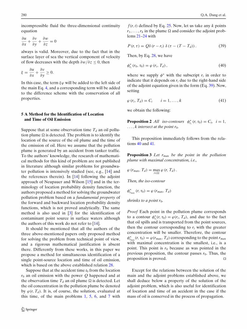
Fig. 17 Profile of concentration in adjoint mode for the sourceat r1
under the assumption that the velocity is axially di-rected. In this, the adjoint problem in backward timefor the above main problem has the form
L∗−φ∗ ≡ ∂φ∗
∂τ−U
∂φ∗
∂x+ σφ∗ − μ
∂
∂x
(μ
∂φ∗
∂x
)= P (x, τ )
φ∗ = 0, τ = 0,
φ∗ = 0, x = a, Uφ∗ + μ∂φ∗
∂x= 0, x = b .
By solving the main problem for the right-hand sidef (x, t) = δ(x)δ(t) on the interval [−50, 50] with thediffusion coefficient μ = 0.1, the velocity u = 0.9, spacegrid of 301 nodes, and time step �t = 0.5, we obtain theprofiles of concentration of substance caused by a pointinstantaneous source of the unit power located at x = 0,
Fig. 18 Profile of concentration in adjoint mode for the sourceat r2
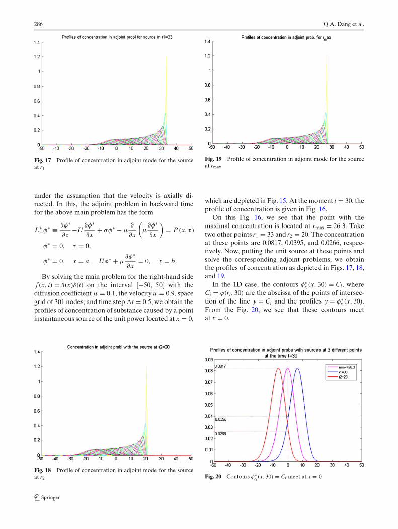
Fig. 19 Profile of concentration in adjoint mode for the sourceat rmax
which are depicted in Fig. 15. At the moment t = 30, theprofile of concentration is given in Fig. 16.
On this Fig. 16, we see that the point with themaximal concentration is located at rmax = 26.3. Taketwo other points r1 = 33 and r2 = 20. The concentrationat these points are 0.0817, 0.0395, and 0.0266, respec-tively. Now, putting the unit source at these points andsolve the corresponding adjoint problems, we obtainthe profiles of concentration as depicted in Figs. 17, 18,and 19.
In the 1D case, the contours φ∗ri(x, 30) = Ci, where
Ci = ϕ(ri, 30) are the abscissa of the points of intersec-tion of the line y = Ci and the profiles y = φ∗
ri(x, 30).
From the Fig. 20, we see that these contours meetat x = 0.
Fig. 20 Contours φ∗ri(x, 30) = Ci meet at x = 0
Numerical Simulation of Oil Pollution Spills 287
Fig. 21 Contours φ∗ri(x, 30) = Ci meet at x = 0
In addition to these three points, we take now thetwo points r3 = 24, r4 = 30 and plot the profiles y =φ∗
ri(x, 30) for all five points r1, r2, rmax, r3, r4 and define
the contours φ∗ri(x, 30) = Ci = ϕ(ri, 30) (see Fig. 21).
Once again we see that these contours meet at x = 0,which is the source location in the main problem. Thus,all results that are proved and demonstrated in the 2Dcase are verified in the 1D case.
8 Conclusion and Outlook
In this work, we considered a mathematical model ofoil spill resulting from a tanker traffic accident and itsnumerical solution. For solving the problem of iden-tification of the source of oil pollution, we use adjointmethod. A fundamental equality between the solutionsof the main and the adjoint problems was proved, andbased on it, a method for the identification problem wasproposed. Some numerical simulations demonstratedthe effectiveness of the method.
Future research directions will include error analysisof the method and applicability of the method in thecase of incomplete information of the total power ofthe source of emission. The case of non-instantaneoussource also will be investigated.
Moreover, we will improve the coastline boundaryconditions by including the shoreline interaction. Sinceonly a certain maximum volume of oil can be depositedat the shoreline, we have consider different types ofcoastlines, cf. [18]
Acknowledgements This first two authors were supported par-tially by the bilateral German–Vietnamese project OILPOLL:
Mathematical Modelling and Numerical Algorithms for Simu-lation of Oil Pollution, financed by the International Buro ofthe BMBF. The third author was supported by the VietnamNational Foundation for Science and Technology Development(NAFOSTED).
References
1. Bagtzoglou, A. C., & Atmadja, J. (2005). Mathematical meth-ods for hydrologic inversion: The case of pollution sourceidentification. Handbook of Environmental Chemistry, 5,65–96.
2. Cacuci, D. G., & Schlesinger, M. E. (1994). On the applicationof the adjoint method of sensitivity analysis to problems in theatmospheric sciences. Atmósfera, 7, 47–59.
3. Cheng, W. P., & Jia, Y. (2010). Identification of contaminantpoint source in surface waters based on backward locationprobability density function method. Advanced Water Re-sources, 33, 397–410.
4. Dang, Q. A. (2002). Monotone difference schemes for solvingsome problems of air pollution. Advances in Natural Sciences,4, 297–307.
5. Dang, Q. A., & Ehrhardt, M. (2006). Adequate numeri-cal solution of air pollution problems by positive differenceschemes on unbounded domains. Mathematical and Com-puter Modelling, 44, 834–856.
6. Dang, Q. A., Ehrhardt, M., Tran, G. J., & Le, D. (2007). Onthe numerical solution of some problems of environmentalpollution. In C. B. Bodine (Ed.), Air pollution research ad-vances (pp. 171–200). Hauppauge: Nova Science.
7. Dimov, I., & Zlatev, Z. (2002). Optimization problems in air-pollution modeling. In P. M. Pardalos, M. G. C. Resende(Eds.), Handbook on applied optimization. Oxford: OxfordUniversity Press.
8. Doerffer, J. W. (1992). Oil spill response in the marine envi-ronment. Oxford: Pergamon.
9. Fay, J. A. (1971). Physical processes in the spread of oil ona water surface. In Proc. conf. prevention and control of oilspills (pp. 463–467). Washington, D.C.: American PetroleumInstitute.
10. Kreiss, H.-O., & Lorenz, J. (1989). Initial-boundary valueproblems and the Navier–Stokes equations. New York:Academic.
11. Lehr, W. J., Fraga, R. J., Belen M. S., & Cekirge, H. M.(1984). A new technique to estimate initial spill size using amodified fay-type spreading formula. Marine Pollution Bul-letin, 15, 326–329.
12. Marchuk, G. I. (1986). Mathematical models in environmentalproblems. New York: Elsevier.
13. Marchuk, G. I. (1995). Adjoint equations and analysis of com-plex systems. Dordrecht: Kluwer.
14. Milnes, E., & Perrochet, P. (2007). Simultaneous iden-tification of a single pollution point-source location and con-tamination time under known flow field conditions. Advancesin Water Resources, 30, 2439–2446.
15. Neupauer, R. M., & Wilson, J. L. (1999). Adjoint method forobtaining backward-in-time location and travel time prob-abilities of a conservative groundwater contaminant. WaterResources Research, 35, 3389–3398.
288 Q.A. Dang et al.
16. Pudykiewicz, J. A. (1998). Application of adjoint tracertransport equations for evaluating source parameters. At-mospheric Environment, 32, 3039–3050.
17. Reed, M., Johansen, Ø., Brandvik, P. J., Daling, P., Lewis,A., Fiocco, R., et al. (1999). Oil spill modeling towards theclose of the 20th century: Overview of the state of the art.Spill Science & Technology Bulletin, 5, 3–16.
18. Reed, M. (2001). Technical description and verification testsof OSCAR2000, a multi-component 3-dimensional oil spillcontingency and response model. SINTEF Applied Chem-istry Report.
19. Samarskii, A. A. (2001). The theory of dif ference schemes.New York: Dekker.
20. Skiba, Y. N. (1995). Direct and adjoint estimates in the oilspill problem. Revista Internacional de Contaminación Ambi-ental, 11, 69–75.
21. Skiba, Y. N. (1996). Dual oil concentration estimates in eco-logically sensitive zones. Environmental Monitoring and As-sessment, 43, 139–151.
22. Skiba, Y. N. (1996). The derivation and applications of theadjoint solutions of a simple thermodynamic limited area
model of the atmosphere–ocean–soil system. World ResourceReview, 8, 98–113.
23. Skiba, Y. N. (1999). Direct and adjoint oil spill estimates.Environmental Monitoring and Assessment, 59, 95–109.
24. Skiba, Y. N., & Parra-Guevara, D. (1999). Mathematics ofoil spills: Existence, uniqueness, and stability of solutions.Geofísica Internacional, 38, 117–124.
25. Skiba, Y. N. (2003). On a method of detecting the industrialplants which violate prescribed emission rates. EcologicalModelling, 159, 125–132.
26. Skiba, Y. N., Parra-Guevara, D., & Belitskaya, D. V. (2005).Air quality assessment and control of emission rates. Envi-ronmental Monitoring and Assessment, 111, 89–112.
27. Wang, H. Q. & Lacroix, M. (1997). Optimal weighting in thefinite difference solution of the convection–dispersion equa-tion. Journal of Hydrology, 200, 228–242.
28. Wang, S.-D., Shen, Y.-M., & Zheng, Y.H. (2005). Two-dimensional numerical simulation for transport and fate ofoil spills in seas. Ocean Engineering, 32, 1556–1571.
29. Yanenko, N. N. (1971). The method of fractional steps.New York: Springer.