Mathematical Modeling of Catalytic Fixed Bed Reactors · MATHEMATICAL MODELING OF CATALYTIC FIXED...

Mathematical Modeling of Catalytic Fixed Bed Reactors

A.A. Iordanidis

2002

Ph.D. thesisUniversity of Twente

Also available in print:http://www.tup.utwente.nl/catalogue/book/index.jsp?isbn=9036517524

T w e n t e U n i v e r s i t y P r e s s

http://www.tup.utwente.nl/catalogue/book/index.jsp?isbn=9036517524

Mathematical Modeling of Catalytic Fixed Bed Reactors

Samenstelling promotiecommissie:

prof. dr. C. Hoede, voorzitter Universiteit Twente/TW

prof. dr. ir. J.H.A. de Smit, secretaris Universiteit Twente/CT

prof. dr. ir. J.A.M. Kuipers, promotor Universiteit Twente/CT

prof. dr. ir. W.P.M. van Swaaij, promotor Universiteit Twente/CT

dr. ir. A.E. Kronberg, assistent promotor Universiteit Twente/CT

prof. dr. ir. G.F. Versteeg Universiteit Twente/CT

prof. dr. ir. J.J.W. van der Vegt Universiteit Twente/TW

prof. dr. ir. K.R. Westerterp Universiteit Twente/CT

dr. ir. A. Stankiewicz DSM Research

dr.ir. M. van Sint Annaland Universiteit Twente/CT

The research reported in this thesis was funded by the Netherlands Organization for Scientific

Research (N.W.O).

Publisher: Twente University Press, P.O. Box 217, 7500 AE Enschede, The Netherlands

www.tup.utwente.nl

Print: Océ Facility Services, Enschede

© A.A. Iordanidis, Enschede, 2002

No part of this book may be reproduced by print, photocopy or any other means without

permission in writing from the publisher.

ISBN 9036517524

MATHEMATICAL MODELING OF CATALYTIC

FIXED BED REACTORS

PROEFSCHRIFT

ter verkrijging van

de graad van doctor aan de Universiteit Twente,

op gezag van de rector magnificus,

prof.dr. F.A. van Vught,

volgens besluit van het College voor Promoties

in het openbaar te verdedigen

op woensdag 26 juni 2002 te 15.00 uur

door

Arthouros Aristotelis Iordanidis

geboren op 23 mei 1973

te Georgia, USSR

Dit proefschrift is goedgekeurd door de promotoren

prof. dr. ir. J.A.M. Kuipers

prof. dr. ir. W.P.M. van Swaaij

to my parents

Aristotelis and Natalia

VI

Contents

Summary ............................................................................................................. 1 Samenvatting ...................................................................................................... 6 1. General Introduction .................................................................................. 11 2. Mathematical models of packed bed reactors. Applicability of different

reactor models................................................................................................... 17 Abstract ............................................................................................................................... 18

2.1 Introduction ................................................................................................................. 19

2.2 Continuum models ...................................................................................................... 21

2.2.1 Two examples of packed bed reactor systems ..................................................... 22

2.2.2 One-dimensional pseudo-homogeneous model ................................................... 24

2.2.3 One-dimensional heterogeneous model ............................................................... 27

2.2.4 One-dimensional pseudo-homogeneous and heterogeneous models with axial

dispersion ........................................................................................................................ 31

2.2.5 Two-dimensional models ..................................................................................... 34

2.2.6 Models accounting for intraparticle resistance. The effectiveness factor ............ 39

2.2.7 Models accounting for the radial porosity distribution ........................................ 45

2.2.8 Dynamic models................................................................................................... 47

2.3 Cell models.................................................................................................................. 49

2.4 Summary and conclusions........................................................................................... 52

Appendix 2.A. – Correlations for transport parameters ...................................................... 54

I. Effective radial thermal conductivity (λer) .................................................................. 54

II Effective radial diffusivity (Der) .................................................................................. 57

III Wall heat transfer coefficient (hw).............................................................................. 58

IV Overall heat transfer coefficient for 1-D model (Uw) ................................................ 59

V Axial heat dispersion coefficient (λez)......................................................................... 60

VI Axial mass dispersion coefficient (Dez) ..................................................................... 60

VII Solid-fluid heat transfer coefficient (hfs)................................................................... 61

VIII Solid-fluid mass transfer coefficient (kf) ................................................................. 62

VII

3. Numerical methods and the package of programs for packed bed

modeling ............................................................................................................ 63 Abstract ............................................................................................................................... 64

3.1 Introduction ................................................................................................................. 65

3.2 Stiffness....................................................................................................................... 66

3.3 Optimization of the system of balance equation ......................................................... 72

3.4 Coupling between solid and fluid phase equations ..................................................... 75

3.5 Solution of systems with diffusion terms.................................................................... 78

3.6. Summary and Conclusions......................................................................................... 82

4. Numerical methods for the solution of the wave and convection

dominated diffusion type models .................................................................... 85 Abstract ............................................................................................................................... 86

4.1 Introduction ................................................................................................................. 87

4.2 Approximation of the convection terms...................................................................... 90

4.2.1 Finite propagation speed and the CFL condition ................................................. 90

4.2.2 Upwind differencing ............................................................................................ 92

4.2.3 Discontinuous solutions and monotone schemes ................................................. 94

4.2.4 Spurious solutions and conservative and consistent numerical schemes............. 97

4.3 The numerical method................................................................................................. 99

4.3.1 ENO scheme for a 1-D scalar equation................................................................ 99

4.3.2 ENO scheme for system of 1-D equations ......................................................... 108

4.3.3 ENO scheme for a 2-D system of equations ...................................................... 113

4.3.4 Development of a numerical method to solve 1-D wave equations................... 115

4.3.5 Incorporation of boundary conditions ................................................................ 118

4.4 Mesh adaptation ........................................................................................................ 123

4.4.1 One-dimensional mesh adaptation ..................................................................... 123

4.4.2 Two-dimensional mesh adaptation..................................................................... 130

4.5 Summary and conclusions......................................................................................... 135

Appendix 4. A ................................................................................................................... 136

I. The two-dimensional non-steady state wave model .................................................. 136

II. A two-dimensional non-steady state SDM............................................................... 142

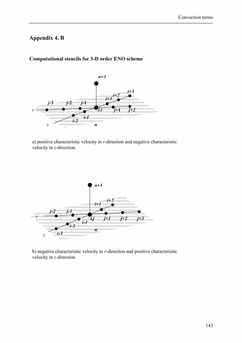
Appendix 4. B ................................................................................................................... 143

VIII

Computational stencils for 3-D order ENO scheme...................................................... 143

Appendix 4. C ................................................................................................................... 144

Application of the ENO method to the energy balance equation of the 1-D non-steady

state pseudo-homogeneous SDM.................................................................................. 144

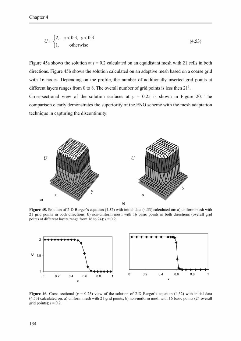
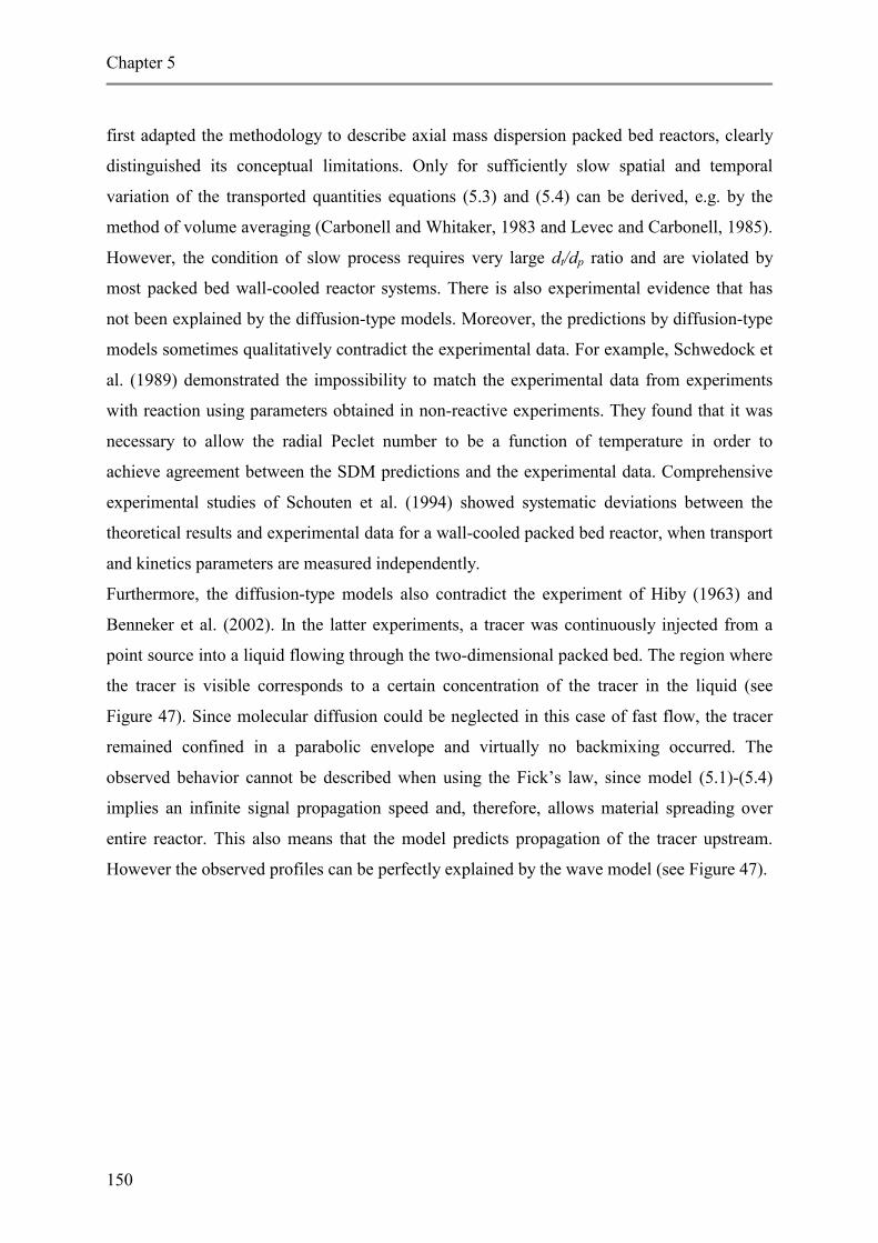
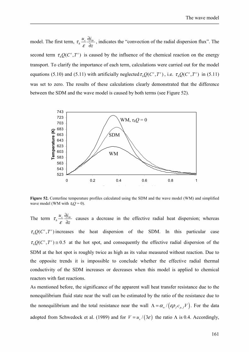
5. The wave model. ..............................................................................................

Experimental validation and comparison with the SDM...................... 147 Abstract ............................................................................................................................. 148

5.1 Introduction ............................................................................................................... 149

5.2 Comparison of the wave model and the SDM with experimental data..................... 155

5.2.1 Two-dimensional steady state models................................................................ 156

5.2.2 One-dimensional non-steady state models......................................................... 164

5.3 Comparison of the wave model and the SDM. Influence of system parameters ...... 167

5.4 Conclusions ............................................................................................................... 173

Appendix 4.A – A simplified derivation of the wave model equations for longitudinal mass

dispersion .......................................................................................................................... 175

References ....................................................................................................... 177 Nomenclature.................................................................................................. 191 Acknowledgmetns…………………………………………………………...193

Summary

1

Summary

When a reactive fluid flows through a catalytically active packed bed, complex chemical and

physical phenomena take place on different scales of the reactor. On the smallest,

intraparticle scale the reactants diffuse, adsorb and react on the active surface of the catalyst

and then desorb and diffuse back to the bulk of the fluid. Convection is the dominant

mechanism of heat and mass transport in the external fluid. The flow pattern is extremely

complex due to the presence of the packing, which, together with diffusion and heat

conduction, leads to the material and heat dispersion.

Exact description of the mentioned interrelated phenomena is virtually impossible and

simplified mathematical models written in terms of average quantities and containing

effective parameters are used instead of the fundamental equations of change. Usually, these

mathematical models consist of the conservation equations in which the dispersion fluxes are

represented in form of Fick and Fourier laws. This approach leads to the conventional

standard dispersion models (SDM). Despite extensive investigation and attempts to justify

and validate the application of different SDM, there is still no universally accepted model and

the subject is still subject for debate.

The complexity of the real processes taking place in packed bed reactors not only leads to

difficulties and uncertainties with their mathematical description, but also to problems with

the numerical handling of the resulting equations. Therefore, the numerical treatment of the

packed bed model equations has been studied and a robust and efficient software package for

packed bed reactor modeling has been developed.

In this thesis predictions by the recently proposed wave models and the SDM have been

compared for several industrial processes in order to indicate the range of applicability of the

models and to identify the most important parameters effecting the differences between the

models. A significant part of the thesis is devoted to the numerical treatment of the packed

bed model equations. A user-friendly software package including conventionally used and

novel wave models has been developed.

Summary

2

SDM versus wave models

The capabilities of the SDM have been investigated based on two industrially important

processes: ethylene oxidation and oxidation of methanol to formaldehyde. The first process

carried out at operating condition considered in this work showed relatively small variations

of temperature and concentrations in the reactor and all the applied models produce very

similar results. In contrast, mathematical modeling of methanol oxidation process revealed

large variations of the temperature and concentrations in the reactor and different models

predicted very different results. Moreover, the SDM was able to describe pilot plant

experimental data only by assuming a temperature dependence of transport parameters, which

does not have any fundamental justification. In addition, the SDM cannot capture basic

phenomena in the packed bed such as propagation of a tracer injected in a flowing liquid

(Hiby, 1963 and Benneker, 2002).

A new wave concept proposed by Westerterp et al. (1995) and Kronberg et al. (1999) was

applied by Benneker et al. (1997, 2002) to describe the tracer injection experiments and

longitudinal dispersion in tubular reactors and produced very encouraging results.

In this thesis the wave models was applied to describe the experimental data for three

processes carried out in packed bed reactors: 1) partial oxidation of methanol to

formaldehyde; 2) synthesis of vinyl acetate from acetic acid and acetylene and 3)

methanation of carbon dioxide.

Partial oxidation of methanol to formaldehyde is accompanied by intensive heat release,

resulting in large spatial variations of the bed temperature (150-200 oC). It has been shown

that the wave model can correctly describe the experimentally data, whereas this particular

process falls out of the range of applicability of the SDM.

The second process, the synthesis of vinyl acetate, also involves both axial and radial

variations of the temperature and concentrations, but the spatial temperature variations are

not very pronounced (only about 10 oC). Both the SDM and the wave model predict similar

results and give a fairly good description of the reported experimental data.

In the third case the dynamic behavior of an adiabatic methanator with mild temperature and

concentration variations in the reactor has been considered. Comparison of the SDM and the

wave model predictions with the experimental data revealed a perfect match of experimental

and calculated temperature and concentration profiles.

Investigation was carried out to determine the parameters responsible for the deviations

between the predictions of the wave models and the SDM. It has been found that they are

Summary

3

mainly due to the differences in the energy balance equations. The deviations between the

models can be significant even in the absence of chemical reaction. Furthermore, the

differences are more pronounced if the ratio dt/dp is small and they are amplified if a

chemical reaction takes place.

Numerical treatment of the packed bed model equations

There are several problems specific for packed bed model equations. The system usually

contains a large number of equations and a large number of source terms (the reaction rates).

The source terms may have very different characteristic times, which results in a stiff system of

differential equations. Furthermore, the model equations usually involve diffusion-type terms,

implicit discretization of which gives sparse matrices. The sparsity of matrices should be

properly addressed in order to construct an efficient numerical solver. Since convection is the

dominant mechanism of material and heat transport, special care should be taken to ensure an

accurate and reliable resolution of the convection terms. This is especially important for the

wave model equations, since they do not contain diffusive terms. When developing the

algorithms for the numerical solution of the model equations it was kept in mind that all the

problems mentioned above should be addressed simultaneously, so that each individual method

that treats specific phenomena should be sufficiently robust and efficient to solve the problem

at hand and simple and flexible enough to allow its incorporation with the other numerical

techniques.

To solve stiff systems of differential equations a method based on the powerful Newton-

Kantorovich approach and accompanied with a simple but effective time step control has

been developed. The method is capable of solving extremely stiff problems with a stiffness

ratio of order 107.

To efficiently deal with the large number of differential equations it is proposed to introduce

key components for each reaction and solve the equations in terms of these new variables

instead of the original concentrations. Among others the beneficial features of the proposed

method are: 1) Automatic selection of linearly independent components from the set of all

components. Conventionally this is done by extraction of a linearly independent submatrix

from the matrix of stochiometric coefficients, which is quite a formidable task if more then 7-

10 reactions are involved. 2) Solution of the minimum possible number of differential

equations, which is equal to the number of reactions.

Summary

4

A new technique has been proposed to efficiently solve heterogeneous model equations. The

technique significantly reduces the required computer resources and simplifies the

implementation of numerical methods by decoupling the fluid and solid phase equations in

such a way that the large system of finite-difference equations is solved in two consecutive

steps. In each step a much smaller system of equations is solved.

Considerable attention has been devoted to the discretization of the convection terms and

incorporation of the diffusion and source terms and the boundary conditions into the

numerical scheme. To assure the reliability of the constructed method, a list of necessary

conditions, reflecting the physical and mathematical features of the system, has been

compiled. It has been demonstrated that violation of any of theses conditions may result in

inaccurate, unstable or, what is the worst, fake but reasonably appearing solutions. The

method is based on the essentially non-oscillatory (ENO) reconstruction of the numerical

fluxes and allows efficient incorporation of the source and diffusive terms and the boundary

conditions. Due to the characteristic decomposition used in the discretization the technique

has been extended with relative ease to two-dimensional packed bed reactor models.

Robustness, accuracy and efficiency of the method in capturing very steep (or discontinuous)

profiles and extrema points, and the advantages in the implementation of the method have

been demonstrated in comparison with most often used methods.

Very often in chemical engineering problems the region of sharp changes of temperature and

concentration profiles is very narrow (e.g. combustion zone). Nevertheless, the size of all

computational cells in an equidistant grid is dictated by the cell size in this region. This leads

to excessively small cells in other regions. To enhance the performance of the proposed

method a mesh adaptation technique has been developed. The technique extensively uses

information calculated for the ENO discretization and thus does not involve much additional

calculations. A crucial feature of the proposed technique is that it does not spoil any of the

beneficial properties of the ENO scheme. Furthermore, the possibility and relative ease with

which the multidimensional grids adaptation can be achieved is undoubtedly another essential

merit of the proposed technique.

Software developed for packed bed modeling

The numerical techniques presented in this thesis, along with many conventionally used

techniques, have been implemented in the software package “PackSim” – a package

especially developed for the mathematical modeling of packed bed reactors. The core of the

Summary

5

package consists of computational units solving certain types of equations by finite-

differencing. The computational units are embedded in a graphical user-friendly interface. A

user is provided with a number of classical continuum models of different complexity as well

as the novel wave models. An arbitrary number of components and arbitrary reaction rate

expressions can be treated with each model. The necessary transport parameters can either be

calculated within the program using embedded correlations or supplied by the users. The

package is developed for both experienced researchers and users with only basic knowledge

of packed bed reactors.

Samenvatting

6

Samenvatting

Waneer een reactief gas of vloeistof door een katalytisch actief gepakt bed stroomt, vindt een

aantal complexe chemische en fysische processen plaats op verschillende schaalniveaus. Op

de kleinste schaal, binnen in de deeltjes, vindt diffusie van reactanten plaats, die vervolgens

reageren op het katalytisch actieve oppervlak. Gevormde producten desorberen van het actief

materiaal en diffunderen uit de deeltjes naar het omringende fluïdum. In de omringende

fluïde fase is convectie het belangrijkste mechanisme voor warmte- en stoftransport. Het

complexe stromingspatroon binnen de pakking zorgt, samen met diffusie en warmtegeleiding,

tot dispersie van massa en warmte.

Een exacte beschrijving van alle, onderling gekoppelde fenomenen is welhaast onmogelijk.

Mathematische modellen voor de beschrijving van gepakte bedden beschrijven de processen

in termen van gemiddelde waarden met behulp van effectieve transportparameters in plaats

van de fundamentele behoudsvergelijkingen. Gewoonlijk bestaan deze wiskundige modellen

uit behoudswetten, waarin de dispersie-fluxen worden berekend volgens de wetten van Fick

en Fourier. Deze benadering leidt tot de conventionele standaard dispersie modellen (SDM).

Ondanks het vele onderzoek en de talrijke pogingen om de aannames, gemaakt in het SDM,

te rechtvaardigen en te valideren, is dit model nog steeds niet algemeen aanvaard.

De complexiteit van de eigenlijke processen die zich afspelen in een gepakt-bed reactor leidt

niet alleen tot onzekerheden in de wiskundige beschrijving ervan, maar ook tot problemen bij

de numerieke oplossing van de resulterende modelvergelijkingen. Daarom is binnen dit

onderzoek aandacht besteed aan de numerieke technieken die worden gebruikt voor het

oplossen van deze vergelijkingen en is een robuust en efficiënt software-pakket ontwikkeld

voor de modellering van gepakt-bed reactoren.

In dit proefschrift worden de resultaten van het recent ontwikkelde wave model vergeleken

met de voorspellingen van het SDM. Een aantal industriële processen wordt hierbij als

voorbeeld gebruikt om aan te geven binnen welk bereik van condities de verschillende

modellen toepasbaar zijn en om de belangrijkste parameters te identificeren die het verschil

in uitkomst tussen de modellen bepalen. Een belangrijk deel van het proefschrift is gewijd

aan de numerieke technieken die worden gebruikt voor het oplossen van de vergelijkingen

Samenvatting

7

van de gepakt-bed modellen. Er is een gebruiksvriendelijk software-pakket ontwikkeld, dat

zowel de alom in gebruik zijnde conventionele modellen als het nieuwe wave model bevat.

SDM versus wave model

De toepasbaarheid van het SDM is onderzocht voor twee belangrijke industriële processen,

namelijk de partiële oxidatie van ethyleen en de oxidatie van methanol tot formaldehyde. De

wiskundige modellering van het eerste, matig exotherme proces (indien uitgevoerd onder de

condities welke worden gebruikt in dit onderzoek), liet zien dat al de gebruikte modellen

sterk overeenkomende resultaten geven. In het geval van de meer exotherme oxidatie van

methanol tot formaldehyde zijn de uitkomsten van de modellen echter zeer verschillend.

Bovendien was het SDM alleen in staat om de experimentele data, gemeten in een pilot plant,

te beschrijven indien de effectieve transportparameters afhankelijk werden verondersteld van

de temperatuur. Hiervoor bestaat echter geen fundamentele verklaring. Een andere

belangrijke tekortkoming van het SDM is dat het geen verklaring kan geven voor eenvoudige

processen in gepakte bedden, zoals de propagatie van een tracer die wordt geïnjecteerd in een

stromende vloeistof (Hiby, 1963 en Benneker, 2002).

Benneker paste de nieuwe wave-benadering, voorgesteld door Westerterp et al. (1995) en

Kronberg et al. (1999), toe voor de beschrijving van tracer-injectie experimenten en van

dispersie in de lengterichting in buisvormige reactoren en vond bemoedigende resultaten

(Benneker et al., 1997, 2002).

In dit proefschrift is het wave model toegepast op de beschrijving van de experimentele data

voor drie processen die worden uitgevoerd in gepakt-bed reactoren: 1) partiële oxidatie van

methanol tot formaldehyde; 2) synthese van vinyl acetaat uit azijnzuur en acetyleen en 3)

methanatie van koolmonoxide.

Tijdens de partiële oxidatie van methanol tot formaldehyde wordt een zeer grote hoeveelheid

warmte geproduceerd, hetgeen leidt tot grote variatie van de bed temperatuur (150-200 °C).

Het is aangetoond dat het wave model de experimentele data goed beschrijft, terwijl dit

proces buiten de toepasbaarheidsgrenzen van het SDM valt.

In het tweede proces, de synthese van vinyl acetaat, ontstaan eveneens temperatuur- en

concentratieverschillen in radiale en axiale richting, maar hier zijn de variaties gering (slechts

ongeveer 10 °C). De voorspellingen van het SDM en het wave model lopen hier nauwelijks

uiteen en geven een redelijk goede beschrijving van de gerapporteerde experimentele data.

Samenvatting

8

In het derde voorbeeld wordt het dynamisch gedrag van een adiabatische methanatie reactor

beschouwd, waarin niet te grote variaties in temperatuur en concentraties voorkomen. Het

SDM en het wave model lieten een perfecte overeenkomst zien met de experimentele

temperatuur- en concentratieprofielen.

Onderzoek is gedaan teneinde de parameters te identificeren welke verantwoordelijk zijn

voor de verschillen tussen de voorspelingen van de wave modellen en het SDM. Het is

gebleken dat deze verschillen hoofdzakelijk worden bepaald door verschillen in de

energiebalans. De modellen onderscheiden zich zelfs bij afwezigheid van chemische reactie.

Verder neemt het verschil tussen de modellen toe wanneer de aspect ratio dt/dp afneemt en

wordt het versterkt wanneer chemische reactie plaatsvindt.

Numerieke behandeling van de modelvergelijkingen van gepakt-bed reactoren

Enkele problemen zijn kenmerkend voor de modelvergelijkingen voor gepakt-bed reactoren.

De modelvergelijkingen bestaan gewoonlijk uit een groot aantal differentiaalvergelijkingen

met brontermen (reactiesnelheden). Deze brontermen kunnen sterk verschillende

karakteristieke tijden hebben, zodat een ‘stijf’ stelsel van differentiaalvergelijkingen

resulteert. Vervolgens kunnen de modelvergelijkingen diffusie-termen bevatten, hetgeen na

discretisatie leidt tot zeer gering gevulde matrices. Hiermee dient rekening te worden

gehouden bij het ontwikkelen van een efficiënte oplosroutine. Aangezien convectief transport

van massa en energie gewoonlijk dominant is in gepakt-bed reactoren, dient speciale

aandacht te worden besteed aan een nauwkeurige en betrouwbare numerieke behandeling van

de convectie-termen. Met name voor het wave model is dit zeer belangrijk, aangezien het

geen diffusie-termen heeft. De verschillende, hierboven beschreven problemen dienen

tegelijkertijd te worden aangepakt. Elke specifieke oplossingstechniek voor de afzonderlijke

problemen dient daarom efficiënt en robuust te zijn, maar tegelijkertijd ook flexibel genoeg

om deze te laten samenwerken met de overige technieken.

Voor het oplossen van stelsels van stijve differentiaalvergelijkingen is een methode

ontwikkeld, die gebaseerd is op de Newton-Kantorovich methode, waarbij de grootte van de

tijdstap op eenvoudige, doch effectieve wijze geoptimaliseerd wordt. De methode werkt zelfs

in het geval van zeer stijve problemen met een ratio in de karakteristieke tijden van 107.

Om op efficiënte wijze te kunnen omgaan met grote stelsels van differentiaalvergelijkingen

wordt voor elke reactievergelijking een sleutel-component geïntroduceerd. Bij het oplossen

van het stelsel van vergelijkingen wordt gerekend met deze sleutelcomponenten in plaats van

Samenvatting

9

de eigenlijke concentraties. De voordelen van deze aanpak zijn onder andere: 1)

Automatische reductie tot een stelsel van onafhankelijke vergelijkingen. Volgens de

traditionele aanpak wordt een lineair onafhankelijke submatrix uit de matrix van

stoïchiometrie-coëfficiënten gedestilleerd, hetgeen zeer omslachtig is indien het aantal

reacties is groter dan 7-10. 2) Het aantal differentiaalvergelijkingen wordt automatisch

gereduceerd tot het minimum aantal, dat gelijk is aan het aantal reacties.

Voor het efficiënt oplossen van de modelvergelijkingen voor heterogene systemen is een

nieuwe techniek ontwikkeld. Deze techniek zorgt voor een besparing op de benodigde

computercapaciteit en vereenvoudigt de implementatie van de numerieke methoden door het

ontkoppelen van de vergelijkingen voor de fluïde en de vaste fase. Met deze nieuwe methode

wordt het grote stelsel van gediscretiseerde differentievergelijkingen in twee opeenvolgende

stappen opgelost, waarbij het aantal vergelijkingen per stap sterk gereduceerd is.

Veel aandacht is gewijd aan de discretisatie van de convectietermen en de integratie van de

diffusie- en brontermen en de randvoorwaarden in het numerieke oplosschema. Om de

betrouwbaarheid van de oplosmethode te garanderen is een lijst van noodzakelijke

voorwaarden opgesteld, die zijn afgeleid uit de fysische en mathematische karakteristieken

van het systeem. Het is aangetoond dat overtreding van deze voorwaarden kan resulteren in

onnauwkeurige of instabiele uitkomsten, of erger nog, dat oplossingen kunnen worden

verkregen die, hoewel ze op het eerste gezicht redelijk lijken, maar fout zijn. De nieuwe

methode is gebaseerd op het ENO (essentially non-oscillatory) schema voor de reconstructie

van de numerieke fluxen en maakt een efficiënte inpassing van de diffusie- en brontermen en

de randvoorwaarden mogelijk. Dankzij de decompositie in karakteristieke variabelen kan

deze methode eenvoudig uitgebreid worden voor het oplossen van twee-dimensionale gepakt-

bed reactor modellen. De robuustheid, nauwkeurigheid en efficiëntie van de methode voor de

beschrijving van extreem steile, of zelfs discontinue profielen zijn aangetoond, evenals de

gemaksvoordelen van toepassing ervan ten opzichte van andere methoden.

In veel gevallen vinden sterke veranderingen van temperatuur en concentratie plaats binnen

een relatief klein gebied in een procesapparaat (bijvoorbeeld een verbrandingszone). In het

geval van een equidistant grid wordt de grootte van de rekencellen over de gehele reactor

bepaald door de maximaal toegestane grootte in dit gebied, waardoor de rekencellen in het

grootste deel van de reactor onnodig klein zijn. Een grid-verfijningstechniek is ontwikkeld

om de efficiëntie van de voorgestelde nieuwe methode te verbeteren door de celgrootte

afhankelijk te maken van de lokale gradiënten. Deze techniek maakt gebruik van dezelfde

Samenvatting

10

informatie die nodig is voor toepassing van de ENO discretisatie en vergt daarom nauwelijks

extra rekenwerk. Een cruciaal kenmerk van de voorgestelde grid-verfijningstechniek is het

feit dat geen van de voordelen van het ENO schema teniet wordt gedaan. Een ander groot

voordeel is het gemak waarmee de techniek kan worden toegepast op problemen in meerdere

dimensies.

Ontwikkelde software voor modellering van gepakte bedden

De nieuwe, in dit proefschrift beschreven numerieke technieken en een groot aantal

conventionele technieken zijn geïmplementeerd in een softwarepakket genaamd “PackSim” -

een pakket dat speciaal is ontwikkeld voor de modellering van gepakt-bed reactoren. De kern

van het programma wordt gevormd door een aantal onderdelen die in staat zijn verschillende

typen differentiaalvergelijken op te lossen met behulp van de eindige-differentie methode.

Deze onderdelen zijn verborgen achter een grafisch, gebruiksvriendelijk gebruikersscherm.

De gebruiker kan kiezen uit een aantal klassieke continuum-modellen van verschillende

complexiteit en uit de nieuwe wave modellen. In elk model kan een onbeperkt aantal

componenten en reacties met willekeurige reactiesnelheidsvergelijkingen worden gebruikt.

De benodigde transportparameters kunnen door het programma zelf worden berekend uit de

literatuur-correlaties die hierin zijn opgenomen, of door de gebruiker zelf worden opgegeven.

Het ontstane softwarepakket is geschikt voor gebruik door zowel ervaren onderzoekers als

door gebruikers met slechts een summiere kennis van gepakt-bed reactoren.

CHAPTER 1

General Introduction

Chapter 1

12

A packed bed catalytic reactor is an assembly of usually uniformly sized catalytic particles,

which are randomly arranged and firmly held in position within a vessel or tube. The

reactants are supplied to the reactor with the bulk of the fluid flowing through the packed

bed. Contacting with the catalytically active particles, the reactants undergo chemical

transformations, which are usually accompanied with heat release or heat consumption. If

necessary, the heat is removed or supplied through the tube wall.

The first commercial application of a packed bed reactor dates from 1831 when Peregine

Philips, a British vinegar maker, patented a process for making sulfur trioxide by passing air

and sulfur dioxide over a hot bed of platinum sponge. Since the catalyst was not consumed in

the reaction, it could be used repeatedly as a continuous flow of reactants was passed over the

bed, without the need for separating and recycling the catalyst.

Since then, packed bed catalytic reactors have become one of most often used units for gas-

solid and liquid-solid reactions. Despite of the existence of newer types of reactors such as

fluidized bed reactors, the packed bed reactors are widely used for large scale processing in

petroleum industry (e.g. catalytic reforming and hydro-treatment) and basic chemical industry

(e.g. ammonia and sulfuric acid synthesis).

When the fluid containing the reactants flows through the packed bed a variety of physical

and chemical phenomena occur in the reactor. Due to enormous complexity of these

phenomena an exact mathematical description of packed bed reactors is virtually impossible

and simplified mathematical models in terms of averaged quantities have been developed for

their description.

In 1950 Bernard and Wilhelm described radial dispersion in packed beds by a Fickian model.

In 1953 Danckwerts published his celebrated paper on residence time distribution in

continuous contacting vessels, including chemical reactors, and thus provided methods for

measuring axial dispersion rates. These important contributions has set the direction in which

the mathematical modeling of packed bed reactors have been developing. Up till now the

continuum type models are the most often used for the description of packed bed reactors.

The models are based on the conservation laws for material, energy and momentum and lead

to differential and/or algebraic equations. The complexity of a model depends on the

simplifying assumptions made which are determined by many factors. Firstly, it depends on


13

the considered problem and on the particular phenomena dictating its most crucial features.

Secondly, it depends on the accuracy of the available transport and kinetic parameters. An

important feature of any mathematical model is its feasibility for mathematical treatment of

the model equations. Therefore, it is widely accepted that there is no universal packed bed

reactor model and each problem should be carefully analyzed to identify permissible

simplifying assumptions. It should be investigated whether the reactor can be considered as a

pseudo-homogeneous continuum with averaged properties. If the differences between the

fluid and solid phase conditions are significant, heterogeneous models have to be considered.

Moreover, it should be examined whether it is necessary to explicitly account for intraparticle

resistances to heat and mass transport.

Despite extensive investigation of packed bed reactors and efforts to mathematically model

them, there is still a lack of fundamental justification of the conventionally used continuum

models, which employ a Fick and Fourier type description for the mass and heat dispersion

fluxes respectively. Moreover, there is experimental evidence that cannot be explained with

the standard dispersion models and is even contradicting to this approach.

Recently a new wave concept of hydrodynamical dispersion has been proposed by Westerterp

et al. (1996) to overcome some of the conceptual shortcoming of the conventional one-

dimensional continuum models. The wave model has been applied for the description of

longitudinal mass and heat dispersion in tubular reactors by Benneker et al. (1997) and

revealed the capabilities of the new approach to describe the processes in a physically sound

way. Later Kronberg et al. (1999) extended the approach to describe two-dimensional heat

and material transport processes in packed bed reactors. Visualization experiments and the

application of the new wave and conventional diffusion type models to describe the

experimental results obtained by Benneker et al. (2002) clearly demonstrated the advantages

of the wave models and encouraged the application of the wave models to packed bed

reactors.

In addition to the problems associated with the formal, mathematical description of packed

bed reactors, mathematical treatment of the governing model equations should also be

carefully addresses. Due to the strong non-linearity of the reaction rate expressions, an

analytical solution of the system of differential/algebraic equations can rarely be obtained.

Therefore, the focus is usually on the numerical, approximate, solution of the equations.

Chapter 1

14

There are several numerical problems specific for the packed bed reactor model equations.

Usually models include a large number of partial differential equations. Due to a variety of

chemical and physical processes reflected in the model equations, a number of numerical

techniques should be employed simultaneously. The presence of nonlinear reaction rate

expressions with a possibly wide range of characteristic times for different reactions requires

a robust solver for stiff equations. Discretization of diffusive terms usually produces a set of

linear equations involving very sparse matrices. An efficient solver proposed here takes this

sparsity into account. Since convection is usually the dominant mechanism of material and

heat transport, special attention should be devoted for the discretization of the convection

terms. This is especially important for the wave model equations, which do not contain

diffusion terms (since dispersion is described by mixing of streams convected with different

velocities). Furthermore, to perform efficiently the numerical method should adjust itself

taking into account the properties of the calculated solution, i.e. the computational mesh and

marching step size should be automatically adapted. Finally, note that in order to combine

different techniques treating different phenomena (referred by different terms in the

equations) in one algorithm that solves the entire set of equations, each individual technique

should be flexible and simple enough to allow incorporation in a large program and at the

same should be robust and efficient enough to solve the problem in reliable and efficient way.

Many powerful numerical methods have been developed to solve equations of mathematical

physics including packed bed model equations. Ordinary differential equations are very often

solved a.o. by Runge-Kutta technique or Gear’s (1971) method. Parabolic partial differential

equations are often transformed to ordinary differential equation by using the method of lines

(see, e.g. Schiesser, 1991). Collocation methods are also widely used for solution of packed

bed model equations (Villandsen and Stewart, 1967 and Finlayson, 1972). Powerful methods

for solution of nonlinear boundary-value problems were presented by Kubicek and Hlavacek

(1983).

This work is focused on the numerical problems for packed bed model equations, which have

not been properly addressed before, e.g. solution of wave model equations, tracking of

reaction fronts or discontinuities when diffusion effects are negligible, development of mesh

adaptation techniques for one-dimensional and multidimensional problems, Incorporation of

several robust techniques for the numerical treatment of different individual phenomena in

one general method. Special attention is devoted to optimize the available techniques. Most


15

of the optimization procedures can be incorporated with the above-listed classical numerical

methods.

The presented methods along with the classical numerical methods are used in a software

package, PackSim, designed for the mathematical modeling of packed bed reactors. The

package includes a variety of classical standard dispersion models as well as novel wave

models.

Using the developed methods, the wave models equations are solved in order to compare

their prediction to the predictions of the standard dispersion models and to experimental data.

Several important processes have been considered to identify the conditions when the both

models can be applied for packed bed description and the conditions when the predictions of

the models deviate.

Finally, it should be noted that in this thesis term “packed bed reactor” means a single tube

packed with catalytic particles. However, in industrial cooled or heated packed bed reactors a

bundle of tubes filled with catalyst is usually arranged within a large reactor shell. A fluid

circulating in the exterior of the tubes removes or supplies heat to the packed tubes. Ideally it

is assumed that the tube wall is kept at desired temperature and that all the tubes operate in

the same conditions. However, in practice the shell side of the reactor may have a significant

effect on the reactor performance. Investigation of the multitubular packed bed reactors is out

of the scope of this thesis. Analysis of heat transfer problems and shell side hydrodynamics in

multitubular reactors can be found in Stankiewicz eta al. (1986) and Stankiewicz (1989).

In the following the outline of this thesis is given.

Chapter 2 describes the mathematical models used for the modeling of packed bed catalytic

reactors. The attention is focused on the most widely used continuum models. Applicability

of different continuum models is investigated on the basis of two industrially important

processes: the ethylene oxidation and the oxidation of methanol to formaldehyde. It will be

shown that for highly exothermic processes the discrepancies between the predictions of

different models can be substantial. In certain cases conventional diffusion-type models also

fail to explain experimental data.

Chapter 3 deals with numerical problems specific for the solution of packed bed model

equations. A new technique will be proposed to efficiently handle a large number of stiff

Chapter 1

16

equations. The technique minimizes the number of equations to be solved by introduction of

new variables instead of original concentrations. The technique leads to significant reductions

in computational time and required computer resources. Numerical methods to handle the

discretizations of the diffusive terms and to incorporate heterogeneity of the system are also

presented in chapter 3.

Chapter 4 presents a complete algorithm for the discretization of convection terms for

multidimensional nonlinear systems of partial differential equations. A rigorous analysis is

carried out in order to assure that the developed method does not produce inaccurate or fake

solutions. The capabilities of the method will be compared with the capabilities of the most

widely used discretization methods. An algorithm for 1-D and 2-D computational mesh

adaptation is also presented in this chapter. The technique extensively uses data already

calculated during the discretization of the convective terms and preserves all the beneficial

properties of the discretization.

In Chapter 5 the recently proposed wave model is investigated. The predictions of the wave

model are compared with the predictions of standard dispersion models and experimental

data for three industrially important processes differing in the amount of heat released during

the reactions. Furthermore, a sensitivity analysis will be carried out to determine the

parameters responsible for differences between the predictions of the wave and standard

dispersion models.

A limited version of PackSim, the software package developed in this work for modeling of

packed bed reactors, has been supplied on a CD enclosed to this thesis. The package includes

the most accepted continuum models as well as the novel wave models. The program has

been built on the basis of computational units designed for robust and efficient solution of

different model equations (or different types of partial and ordinary differential equations).

The techniques described in Chapters 3 and 4 along with conventional numerical techniques

was implemented in the program. The package was developed in Borland Delphi and has

been provided with a visualized user-friendly interface to enter reactor data and inspect the

calculated results. The package was designed both for users with deep knowledge of packed

bed reactor modeling and for users without large experience.

CHAPTER 2 ___________________________________________________________________________

Mathematical models of packed bed reactors. Applicability of

different reactor models

___________________________________________________________________________

Chapter 2

Abstract A classification of mathematical models used for description of the packed bed catalytic

reactors is given. The focus was on the most widely used continuum models. Applicability of

different models is investigated on the basis of two industrially important processes. The first

process, the partial oxidation of ethylene, reveals moderately smooth temperature and

concentration profiles and is fairly well described by the pseudo-homogeneous plug flow

model. The discrepancies between the predictions of this simple model and more complicated

two-dimensional heterogeneous models are not very pronounced. It is not the case for the

second process, the partial oxidation of methanol to formaldehyde. Different continuum

models applied to this particular system showed a wide spread in the produced results.

Mathematical description of the reactor by standard dispersion models were not satisfactory

even if very detailed models (two-dimensional heterogeneous model accounting for

intraparticle resistance to heat and mass transfer) were employed. All the applied standard

dispersion models failed to explain pilot-plant reactor experimental data of Schwedock et al.

(1989). The reason of such a discrepancy is expected to be in inherent shortcomings of

diffusion-type approach. The wave model is advocated for the modeling of such intensive

processes.

Mathematical models

19

Equation Section 22.1 Introduction

A packed bed catalytic reactor is an assembly of usually uniformly sized catalytic particles,

which are randomly arranged and firmly held in position within a vessel or tube. The bulk

fluid flows through the voids of the bed. The reactants are transported firstly from the bulk of

the fluid to the catalyst surface, then through catalyst pores, where the reactants adsorb on the

surface of the pores and then undergo chemical transformation. The formed products desorb

and are transported back into fluid bulk. Convection of the bulk fluid is tied in with heat and

mass dispersion. Dispersion effects are largely caused by the complex flow patterns in the

reactor induced by the presence of the packing. Also, the dispersion effects caused by

transport phenomena like molecular diffusion, thermal conduction in fluid and solid phases

and radiation. In most cases chemical reactions are accompanied with heat generation or

consumption. In case of pronounced heat effects the heat is removed or supplied through the

tube wall.

Due to the complex physical-chemical phenomena taking place in packed bed reactors, their

exact description is either impossible or leads to very complex mathematical problems. The

more detailed the mathematical model, the more parameters it will contain. However, many

elementary processes taking place in the reactor can hardly be individually and independently

investigated, only effective parameters can be measured. Thus, the more detailed models

suffer from a lack of accurate parameter estimations. Therefore, for the description of most

chemical reactors, we have to rely on simplified models capturing the most crucial and salient

features of the problem at hand. This, also means that there is no universal model. The best

model is selected on the basis of the properties of the particular system under consideration,

the features of the system one is interested in, the availability of the parameters included in

the model and the prospects of successful numerical treatment of the model equations. There

are several classes of models used for the description of the packed-bed reactors. The first

and most commonly used class of packed bed reactor models is continuum models. In this

type of models the heterogeneous system is treated as a one – or multi-phase continuum. The

continuum approach results in a set of differential-algebraic equations for the bulk fluid and

solid phase variables (Damkohler, 1936, Danckwerts, 1953; Hlavacek and Vortuba, 1977 and

Froment and Bischoff, 1979). According to the second approach, each catalyst pellet along

with its neighboring bulk fluid is considered as a reactor unit or cell. Each cell is connected

with some of the neighboring cells. Networks of cells and interaction between them form the

Chapter 2

20

so-called cell models (Deans and Lapidus, 1960; McGuire and Lapidus, 1965; Vanderveen et

al., 1968; Hlavacek and Vortuba, 1977). The transport processes taken into account determine

the way the neighboring cells interact and, consequently, the type of cell model. Finally, a

group of models incorporates experimentally measured distribution of the void fraction

(porosity) in the mathematical description. These models where formerly referred to as

channel models. The local porosity is maximal near the wall and decreases in the direction

towards the tube axis in an oscillatory manner with a period of about 1-2 particle diameters.

In a distance of about 4-5 particles the influence of the wall on local porosity vanishes.

Channel models assume that the packed bed is separated by coaxial cylindrical surfaces

passing through places where the free volume reaches minimum values. These surfaces

divide the reactor into a set of coaxial annular channels. Each channel is considered as a plug

flow reactor where the fluid velocity is determined by the average porosity of the channel,

and which exchange heat and mass with neighboring channels. Therefore, channel models

can be regarded as generalizations of classical continuum models. All the advantages and

disadvantages of classical continuum models are inherited by channel models. Since channel

models are not supported with enough engineering data, they have not gained much attention

in packed bed reactor modeling.

Although each type of models has its potentials and drawbacks, packed bed reactors have

been mainly modeled and optimized using continuum models. One of the reasons for that is

the fact that former mass and heat transfer experiments have been analyzed almost

exclusively on the basis of continuum models, and consequently, parameter values are

directly available for continuum models. The second reason is that non-linear reaction rates

can sometimes be handled easier in differential equations compared to algebraic equations,

although advanced numerical methods for non-linear differential equations include

techniques used for solution of non-linear algebraic equations. Therefore, the present work

focuses on continuum models and their numerical treatment.

In the next section a classification of the continuum models is presented, and the applicability

of each model is discussed via numerical simulation of two industrially important processes.

Section 2.3 briefly discusses cell models. The analogy between cell models and finite

difference approximations of continuum models is discussed.

Mathematical models

21

2.2 Continuum models

To simulate a packed bed reactor, appropriate reaction rate expressions are required and the

transport phenomena occurring in the catalyst pellet, bulk fluid and their interfaces need to be

modeled. These phenomena can be classified into the following categories:

• Intraparticle diffusion of heat and mass

• Heat and mass exchange between catalyst pellet and bulk fluid

• Convection of the fluid

• Heat and mass dispersion in the fluid phase

• Thermal conduction in the solid phase

• Heat exchange with the confining walls

The degree of sophistication of the model is determined by the accepted assumptions and,

consequently, by the way how aforementioned phenomena are incorporated in the model.

According to the classification given by Froment and Bishoff (1979), which is widely

accepted in the chemical engineering society, the continuum models can be divided in two

categories: pseudo-homogeneous and heterogeneous models.

In pseudo-homogeneous models it is assumed that the catalyst surface is totally exposed to

the bulk fluid conditions, i.e. that there are no fluid-to-particle heat and mass transfer

resistances. On the other side, heterogeneous models take conservation equations for both

phases into account separately. A general schematic classification of continuum models is

given in Table 2.1.

In addition to the models shown in Table 2.1, many different modifications and combinations

are possible. It is common to incorporate dispersion processes in the energy balance and

neglect them in the mass balances, to relate axial dispersion to either of the phases or to the

both of them, to consider only intraparticle material diffusion assuming isothermal conditions

in the pellet, to consider only interface resistance for the heat transfer. The continuum models

indicated in Table 2.1 and their range of applicability will be discussed in what is followed.

The comparison between the models is done based on two examples given in the next section.

Chapter 2

22

Table 2.1. Classification of classical continuum models.

2.2.1 Two examples of packed bed reactor systems

Example I is a simplified reaction model for the partial oxidation of ethylene. The data have

been adopted from Westerterp and Ptasinski (1984). The reaction takes place in excess of

ethylene. Two main by-products CO2 and H2O are formed according to the following reaction

scheme:

R1

R2

R3 C2H4

C2H4O

CO2 + H2O

Pseu

do-h

omog

eneo

us

Heterogeneous

1-D, plug-flow

1-D, axial dispersion

2-D, axial and radial dispersion

2-D, plug-flow, radial dispersion

Intraparticle resistances

Continuum models

Incorporation of the effectiveness factor

Velocity profile Velo

city

pro

file

Mathematical models

23

Under industrial conditions (10 bar and at 200-250 oC, with maximal temperature rise in the

reactor about 20-40 oC) the parallel reactions are dominant and the combustion of ethylene

oxide can be neglected. Thus, the simplified reaction scheme reads:

1

2

2 2 4 2 4

2 2 4 2 2

O + 2C H 2C H O1 1 2O + C H CO H O3 3 3

R

R

→

→ +

The reaction rate expressions are given by

21 1 0=810 CR k , k1 = 70.4 exp(-59860/R/T)

22 2 0=2430 CR k , k2 = 49400 exp(-89791/R/T)

This is a moderate reaction system with smooth temperature and concentration profiles in the

reactor.

Example II represents partial oxidation of methanol to formaldehyde. The data used in this

example are obtained from pilot plant reactor experiments reported by Windes et al. (1989).

The reaction is carried out on commercial iron-oxide/molybdenum-oxide catalyst in excess of

oxygen at atmospheric pressure and at 250-400 oC.

The desired reaction

13 2 2 2

1CH OH + O 2CH O + H O2

R→

is accompanied with an undesirable consecutive reaction

22 2 2

1CH O + O CO + H O2

R→

Here 0.5

1 31 0.5

2 31CH OH

CH OH

k CRk C

=+

, k1 = 125⋅107 exp(-79496/R/T), k2 = 1.12⋅exp(-8368/R/T)

0.5

3 22 0.5

21 0.2CH O

CH O

k CRC

=+

, k3 = 54⋅105 exp(-66944/R/T)

The observed temperature rise in the reactor was up to 150-200 oC. These severe operating

conditions make a priory modeling of the system very complicated. Nevertheless, the high

sensitivity of the selectivity to variations in temperature and the danger of moving into a run

away region necessitate careful modeling of the system. The data used for the modeling of

systems I and II are given in Table 2.2.

Chapter 2

24

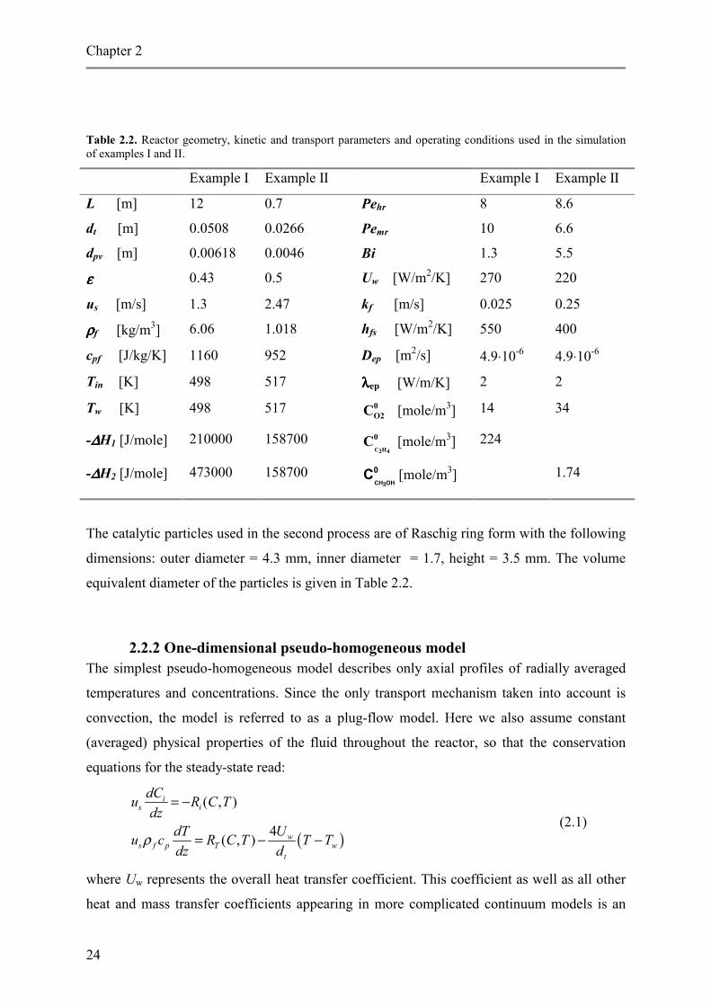
Table 2.2. Reactor geometry, kinetic and transport parameters and operating conditions used in the simulation of examples I and II.

Example I Example II Example I Example II

L [m] 12 0.7 Pehr 8 8.6

dt [m] 0.0508 0.0266 Pemr 10 6.6

dpv [m] 0.00618 0.0046 Bi 1.3 5.5

εεεε 0.43 0.5 Uw [W/m2/K] 270 220

us [m/s] 1.3 2.47 kf [m/s] 0.025 0.25

ρρρρf [kg/m3] 6.06 1.018 hfs [W/m2/K] 550 400

cpf [J/kg/K] 1160 952 Dep [m2/s] 4.9⋅10-6 4.9⋅10-6

Tin [K] 498 517 λλλλep [W/m/K] 2 2

Tw [K] 498 517 0O2C [mole/m3] 14 34

-∆∆∆∆H1 [J/mole] 210000 158700 C H2 4

0C [mole/m3] 224

-∆∆∆∆H2 [J/mole] 473000 158700 CH OH3

0C [mole/m3] 1.74

The catalytic particles used in the second process are of Raschig ring form with the following

dimensions: outer diameter = 4.3 mm, inner diameter = 1.7, height = 3.5 mm. The volume

equivalent diameter of the particles is given in Table 2.2.

2.2.2 One-dimensional pseudo-homogeneous model The simplest pseudo-homogeneous model describes only axial profiles of radially averaged

temperatures and concentrations. Since the only transport mechanism taken into account is

convection, the model is referred to as a plug-flow model. Here we also assume constant

(averaged) physical properties of the fluid throughout the reactor, so that the conservation

equations for the steady-state read:

( )

( , )

4( , )

is i

ws f p T w

t

dCu R C Tdz

dT Uu c R C T T Tdz d

ρ

= −

= − − (2.1)

where Uw represents the overall heat transfer coefficient. This coefficient as well as all other

heat and mass transfer coefficients appearing in more complicated continuum models is an

Mathematical models

25

effective parameter and is calculated using (semi-)empirical correlations. The trustworthiness

of these approximations is crucial for accurate modeling of the packed bed. The most widely

used correlations with the literature references are provided in Appendix 2.A. (See also

Kulkarni and Doraiswamy, 1980; Westerterp et al., 1987 and Stankiewicz ,1989).

In addition to temperature and concentration distributions in the packed bed, the pressure

drop over the reactor is an important reactor characteristic. The pressure drop is rarely more

than 10% of the total pressure. Considering inaccuracies in the reaction rate expressions and

the uncertainties in the transport parameters, the pressure drop does not usually have a

significant effect on the overall model performance. Nevertheless, the pressure drop might be

of great importance for assessment of the reactor operation costs. Pressure drop is calculated

according to the following equation:

2 1 4

2s

h

dP u fdz d

ρ− = (2.2)

Because of the tortuousity of the fluid path and uncertainties with the hydraulic radius of

packed bed, empirical equations are employed to calculate the friction factor f. The most

widely used correlation is the Ergun equation (Ergun, 1949 and 1952):

( ) ( )3

1 12 Reh

fε α ε

βε

− −= +

(2.3)

with α = 150 and β = 1.75. According to MacDonald et al. (1979) the values of α should be

180 and β = 1.8 and 4.0 for smooth and rough pellets respectively.

According to Handley and Heggs (1968) α = 368 and β = 1.24. The results of Ergun and

Handley and Heggs have been reviewed by Hicks (1970). It may be concluded from his work

that the Ergun equation is limited to Reh/(1-ε) < 500 and Handley and Heggs’ to 1000 <

Reh/(1-ε) < 5000. Extensive work on pressure drop in packed beds with particles of various

shapes was done by Leva (1948). He suggested the following correlations for the friction

factor:

( )2

3

1100

Reh

fε

ε−

= for laminar flow

Chapter 2

26

( )1.1

0.13

1 11.75Reh

fεε−

= for turbulent flow

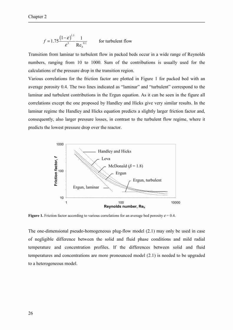
Transition from laminar to turbulent flow in packed beds occur in a wide range of Reynolds

numbers, ranging from 10 to 1000. Sum of the contributions is usually used for the

calculations of the pressure drop in the transition region.

Various correlations for the friction factor are plotted in Figure 1 for packed bed with an

average porosity 0.4. The two lines indicated as “laminar” and “turbulent” correspond to the

laminar and turbulent contributions in the Ergun equation. As it can be seen in the figure all

correlations except the one proposed by Handley and Hicks give very similar results. In the

laminar regime the Handley and Hicks equation predicts a slightly larger friction factor and,

consequently, also larger pressure losses, in contrast to the turbulent flow regime, where it

predicts the lowest pressure drop over the reactor.

Figure 1. Friction factor according to various correlations for an average bed porosity ε = 0.4.

The one-dimensional pseudo-homogeneous plug-flow model (2.1) may only be used in case

of negligible difference between the solid and fluid phase conditions and mild radial

temperature and concentration profiles. If the differences between solid and fluid

temperatures and concentrations are more pronounced model (2.1) is needed to be upgraded

to a heterogeneous model.

10

100

1000

1 100 10000Reynolds number, Reh

Fric

tion

fact

or, f Leva

McDonald (β = 1.8) Ergun

Handley and Hicks

Ergun, laminar Ergun, turbulent

Mathematical models

27

2.2.3 One-dimensional heterogeneous model The simplest one-dimensional heterogeneous model, taking into account temperature and

concentration differences between the fluid bulk and catalyst surface reads:

Fluid phase:

( )( ) ( )4

i

sis f v i

ws f p f v s w

t

dCu k a C Cdz

dT Uu c h a T T T Tdz d

ρ

= −

= − − − (2.4)

Solid phase:

( )( )

( , )

( , )i

s s sf v i i

s s sf v T

k a C C R C T

h a T T R C T

− = −

− = (2.5)

A criterion for determining the onset of interphase heat transfer limitation was derived by

Mears (1971) for the Arrhenius type of reaction rate dependency on the temperature and

under the assumption of negligible direct thermal conduction between spherical particles and

negligible interphase mass transfer resistance. The criterion states that the actual reaction rate

deviates less than 5% from the reaction rate calculated assuming identical solid phase and

bulk fluid conditions, if the following inequality is satisfied:

0.15T p t

f

R d d Th T E

< (2.6)

Extending the idea of Mears to an arbitrary reaction scheme and particle shape the following

deviation between the reaction rates can be obtained:

( ) ( )( )

( ), , , ( , )( , ),

s

s s sT T T T

ssf v TT T T

R T C R T C R T C R T CdeviationT h a R T CR T C

=

− ∂= =

∂ (2.7)

The 5% difference criteria reads deviation < 0.05.

A similar criterion for the interphase concentration difference was derived by Hudgins

(1972). Ri(C,T) and ( )TCR si , do not differ by more than 5% provided that

( ) 0.152

i

i p i

i i f i C C

R d RR C k C

=

∂ <∂

(2.8)

Chapter 2

28

The difference between one-dimensional pseudo-homogeneous and heterogeneous models is

discussed using the aforementioned examples.

The axial temperature and concentration profiles for example I calculated using the 1-D

pseudo-homogeneous model (2.1) are plotted in Figure 2.

Figure 2. Partial oxidation of ethylene (Example I, Table 2.2). Axial temperature and C2H4O concentration profiles calculated using the 1-D pseudo-homogeneous plug flow model (2.1).

The deviation calculated according to (2.7) and using the calculated temperature and

concentrations profiles indicates that the difference in the heat production calculated by

homogeneous and heterogeneous models is less than 6%, see Figure 3. The lower line is

calculated on the basis of the homogeneous model, i.e. (2.7) is calculated assuming sT T= and T

is calculatedby the pseudo-homogeneous model (2.1). The upper line is obtained using the

fluid temperature and concentration profiles predicted by the heterogeneous model (2.4),

(2.5). The more accurate heterogeneous model predicts somewhat larger difference. The axial

temperature and concentration profiles for the two models are compared in Figure 4.

495

500

505

510

515

520

0 0.2 0.4 0.6 0.8 1Dimensionless axial position

Tem

pera

ture

(K)

0

1

2

3

4

5

C2H

4O (m

ole/

m3)

C2H4O concentration

Temperature

Mathematical models

29

498

503

508

513

518

523


Tem

pera

ture

(K)

Heterog., fluidHeterog., solid

Homogeneous 0

1

2

3

4

5


C2H

4O (m

ole/

m3)

Homogeneous

Heterog.,fluid

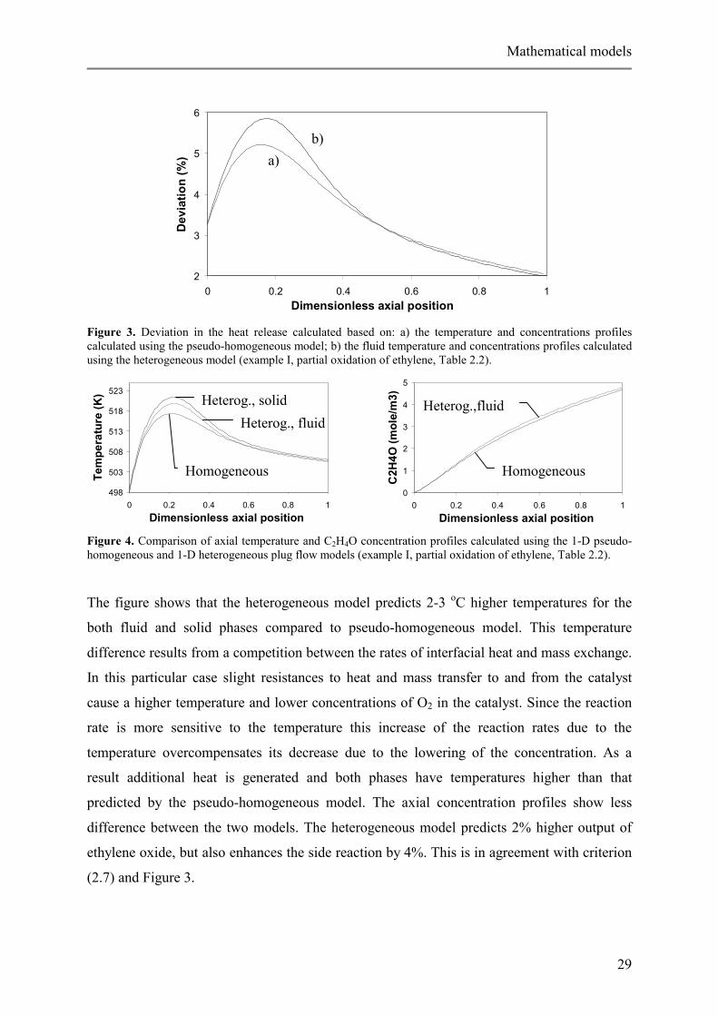
Figure 3. Deviation in the heat release calculated based on: a) the temperature and concentrations profiles calculated using the pseudo-homogeneous model; b) the fluid temperature and concentrations profiles calculated using the heterogeneous model (example I, partial oxidation of ethylene, Table 2.2).

Figure 4. Comparison of axial temperature and C2H4O concentration profiles calculated using the 1-D pseudo-homogeneous and 1-D heterogeneous plug flow models (example I, partial oxidation of ethylene, Table 2.2).

The figure shows that the heterogeneous model predicts 2-3 oC higher temperatures for the

both fluid and solid phases compared to pseudo-homogeneous model. This temperature

difference results from a competition between the rates of interfacial heat and mass exchange.

In this particular case slight resistances to heat and mass transfer to and from the catalyst

cause a higher temperature and lower concentrations of O2 in the catalyst. Since the reaction

rate is more sensitive to the temperature this increase of the reaction rates due to the

temperature overcompensates its decrease due to the lowering of the concentration. As a

result additional heat is generated and both phases have temperatures higher than that

predicted by the pseudo-homogeneous model. The axial concentration profiles show less

difference between the two models. The heterogeneous model predicts 2% higher output of

ethylene oxide, but also enhances the side reaction by 4%. This is in agreement with criterion

(2.7) and Figure 3.

2

3

4

5

6


Dev

iatio

n (%

)

b) a)

Chapter 2

30

500

520

540

560

580

600

620

640


Tem

pera

ture

(K) Heter., solid

Heter., fluid

Homog.

0

0.5

1

1.5

2


CH

3OH

(mol

e/m

3)

Homog.

Heterog., fluid

Larger differences between pseudo-homogeneous and heterogeneous models are expected for

the second example. Calculation of the deviation (2.7) for example II predicts over 10 %

discrepancy between the two models, as illustrated in Figure 5.

Figure 5. Deviation of the heat release calculated using the heterogeneous model from the heat release calculated using the pseudo-homogeneous model (example I, partial oxidation of ethylene, Table 2.2).

Indeed, the axial temperature profiles plotted in Figure 6 show about 30 oC difference in the

hot spot temperatures. The position of the hot spot predicted by the heterogeneous model is

shifted towards the reactor inlet. This is explained by the faster methanol conversion for

heterogeneous model due to the higher temperatures. The pseudo-homogeneous model

predicts a more gradual methanol conversion, with a stretched reaction zone. The observed

discrepancies are caused by the resistance to heat transfer from the catalyst surface to the

bulk of the fluid.

Figure 6. Comparison of axial temperature and CH3OH concentration profiles calculated using the 1-D pseudo-homogeneous and 1-D heterogeneous plug flow models (example I, partial oxidation of ethylene, Table 2.2).

0

2

4

6

8

10

12

0 0.2 0.4 0.6 0.8 1Dimensionless radial position

Tem

pera

ture

(K)

Mathematical models

31

0

0.1

0.2

0.3

0.4

0.5


CO

(mol

e/m

3) Heterog., fluid

Homog.

00.20.40.60.8

11.21.41.6


CH

2O (m

ole/

m3)

Homog.

Heterog., fluid

Due to the consecutive reaction scheme, combined with high methanol conversion, this

system is very sensitive to the temperature. The higher the temperature the earlier methanol is

completely converted. In the rest of the reactor only the undesired consecutive reaction takes

place, and as a result, more CO is produced reducing the selectivity of the system, Figure 7.

A comparison of selectivities predicted by the 1-D, 2-D pseudo-homogeneous and

heterogeneous models is given in Figure 14 of section 2.2.5.

Figure 7. Comparison of axial CH2O and CO concentration profiles calculated using the 1-D pseudo-homogeneous and 1-D heterogeneous plug flow models. (example I, partial oxidation of ethylene, Table 2.2).

2.2.4 One-dimensional pseudo-homogeneous and heterogeneous models with axial dispersion

Due to its mathematical simplicity and minimal number of parameters involved, the plug-

flow model is widely used in the chemical engineering community. However, the model

gives only a rough description of the real processes taking place in the reactor. The plug flow

model does not explicitly take into account vital characteristics of packed bed reactors such

as non-uniform temperature and concentration distributions across the bed and mixing

effects, caused by several mechanisms, including mixing due to presence of the packing,

molecular diffusion, thermal conduction, radiation etc. The most common 1-D heterogeneous

model taking dispersion in the fluid phase into account reads:

Fluid phase:

( )

( ) ( )

2

2

2

24

i

si is ez f v i

s ws f p ez f v w

t

dC d Cu D k a C Cdz dz

dT d T Uu c h a T T T Tdz dz d

ρ λ

− = −

− = − − − (2.9)

Solid phase:

Chapter 2

32

( )( )

( , )

( , )i

s s sf v i i

s s sf v T

k a C C R C T

h a T T R C T

− = −

− = (2.10)

The heat and mass dispersion fluxes are described by Fourier’s dzdTj ezhz λ−= and Fick’s

dzdCDj i

ezmz −= laws, respectively. All dispersion effects are lumped in the effective

coefficients ezλ and ezD . According to other models axial dispersion terms are related to the

solid phase (Eigenberger, 1972) or to both phases (De Wasch and Froment, 1971).

As in case of the plug-flow model, equations (2.9) and (2.10) can be approximated by the

corresponding pseudo-homogeneous model. This can be justified if there are no temperature

and concentration differences between the catalyst and the fluid bulk, so that

,s sT T C C≈ ≈ . (2.11)

Vortmeyer and Schaefer (1974) developed an equivalent pseudo-homogeneous description of

the heterogeneous model with axial dispersion in the solid phase. Assuming equal second

derivatives of the fluid bulk and solid phase temperatures

2 2

2 2

sT Tz z∂ ∂=∂ ∂

(2.12)

they derived a pseudo-homogeneous description of non-steady state processes for both gas

and liquid flows. Balakotaiah and Dommeti (1999) contested the less restrictive nature of

(2.12) against (2.11) and exploited the Center Manifold Theory on the theory of dynamic

systems to derive a pseudo-homogeneous model. The full description involves higher order

derivatives of the temperature. Because of the difficulties with physical explanation of higher

order differential equations and the requirement of additional boundary conditions, the

derivatives of order higher than two are not considered there.

Mathematically the axial dispersion model (2.9), (2.10) is a boundary-value problem and

requires boundary conditions both for the inlet and the outlet of the reactor. Danckwerts

(1953) semi-intuitively proposed boundary conditions expressing continuity of fluxes at

steady state:

Inlet:

Mathematical models

33

,0

0

0 : is i s i ez

p s p s ez

dCz u C u C Ddz

dTc u T c u Tdz

ρ ρ λ

= = −

= − (2.13)

Outlet:

0

0:

=

==

dzdTdz

dCLz i

(2.14)

The requirement of boundary conditions at the reactor outlet is a controversial feature of the

axial dispersion model and is caused by the presence of backmixing in this model. The

problem of the formulation of boundary conditions becomes even more troublesome for non-

steady systems. There have been numerous attempts to justify (2.14) or to suggest other

forms of boundary conditions, (e.g. Wehner and Wilhelm, 1956; Pearson, 1959; Van

Cauwenberghe, 1966 and Gunn, 1987). Due to the physical inconsistency of the model in

case of convection dominated dispersion, for which no boundary conditions at the outlet are

required, one can hardly expect trustworthy justification of these conditions.

There is a simple frequently quoted rule for judgment of the relevance of the axial dispersion:

if L/dp > 30 then axial dispersion can be neglected. A more accurate criterion was derived by

Mears (1971) for a single n-th order reaction: the deviation from the plug flow model is less

than 5%, if the following holds:

inlet

outlet

20 lnez

p p s

n D CLd d u C

> (2.15)

For industrial processes this criterion is practically always fulfilled and the axial dispersion

effects may be neglected. Despite of the questionable practical applicability of the axial

dispersion model, it has gained considerable attention in the literature. The axial dispersion

model has many appealing mathematical properties. The system can exhibit multiplicity of

steady states even in the pseudo-homogeneous description, when multiplicity can be caused

only by the axial dispersion terms. Detailed analysis of the regions of multiplicity for short

reactors and equal heat and mass axial Peclet numbers was carried out by Hlavacek and

Hoffman (1970), Varma and Amundson (1973). Later it was shown that the region of

multiplicity is widened for Pemz > Pehz (Hlavacek et al., 1973 and Puszynski et al., 1981), and

that multiplicity can also occur in long packed beds (Vortuba et al., 1972).

Chapter 2

34

All the models described above assume that variation of temperature and concentrations in

the transverse direction can be neglected and that all radial heat resistances can be lumped

into an overall heat transfer coefficient Uw. These serious simplifications can not be justified,

when reactions with a pronounced heat effect are involved and heat is removed or supplied

through the wall. The temperature variations in the radial direction can reach tens of degrees

and can considerably influence the reaction rates. Disregard of the radial temperature and

concentration non-uniformity can lead to substantial miscalculations in important process

characteristics, such as conversion, selectivity, hot spot temperature and its position etc. In

these cases the variations of temperatures and concentrations across the reactor must be

explicitly taken into consideration.

A simple criterion (Mears, 1971a) to determine the importance of radial temperature variation

for the case of Arrhenius type kinetics and negligible axial heat dispersion reads: the

influence of a non-uniform cross section temperature profile on the heat production

(consumption) is less than 5% if ( ) 21 0.4 /4 1 8 /( )

CS t w

er w p t

H R d RT ET d d Biε

λ−∆ −

<+

2.2.5 Two-dimensional models In the two-dimensional model the radial temperature and concentration profiles are accounted

for. The most often used 2-D model is the pseudo-homogeneous model given by equations

( , )

( , )

i er is i

ers f p T

C D Cu r R C Tz r r r

T Tu c r R C Tz r r r

λρ

∂ ∂ ∂ − = − ∂ ∂ ∂

∂ ∂ ∂ − = ∂ ∂ ∂

(2.16)

and accompanied with boundary conditions:

( )

0 00 : ,

0 : 0, 0

/ 2 : 0,

i

i

it w

z C C T TC Trr r

C Tr d Bi T Tr r

= = =∂ ∂= = =∂ ∂∂ ∂= = = − −∂ ∂

(2.17)

Der, and λer are effective radial mass and heat dispersion coefficients obtained from

experiments. For most of the practically important conditions the mass radial Peclet number

Mathematical models

35

495

500

505

510

515

520

525


Tem

pera

ture

(K) 2-D Heter., fluid

1-D Heter., solid

1-D Homog 2-D Homog

0

1

2

3

4

5

6


C2H

4O (m

ole/

m3) 2-D Heter., solid

1-D Heter., solid

2-D Homog.

1-D Homog.

Pemr = usdp/Der is between 8 and 10. Radial heat Peclet number Pehr = usρfcpdp/λer varies in a

wider range. A more detailed discussion of published correlations for radial heat and mass

transport parameters is given in Appendix A.

A heterogeneous version of (2.16) reads:

( )

( )( )( )

( , )

( , )

i

i

si er is f v i

ers f p fs v

s s sf v i i

s s sf v T

C D Cu r k a C Cz r r r

T Tu c r h a T Tz r r r

k a C C R C T

h a T T R C T

λρ

∂ ∂ ∂ − = − ∂ ∂ ∂

∂ ∂ ∂ − = − ∂ ∂ ∂

− = −

− =

(2.18)

The boundary conditions remain the same.

Application of 2-D models to the calculation of the reactor described by Example I gives

results very similar to those obtained with 1-D models, see Figure 8.

Figure 8. Comparison of axial temperature and C2H4O concentration profiles calculated using the 1-D and 2-D pseudo-homogeneous and heterogeneous plug flow models. The 2-D profiles are averaged over the tube cross section (example I, partial oxidation of ethylene, Table 2.2).

The difference between 1-D and 2-D models is virtually negligible. This is due to rather

uniform radial temperature and concentration profiles. Even at the hot spot the temperature

variation in the radial direction does not exceed 10 oC, as shown in Figure 9.

Chapter 2

36

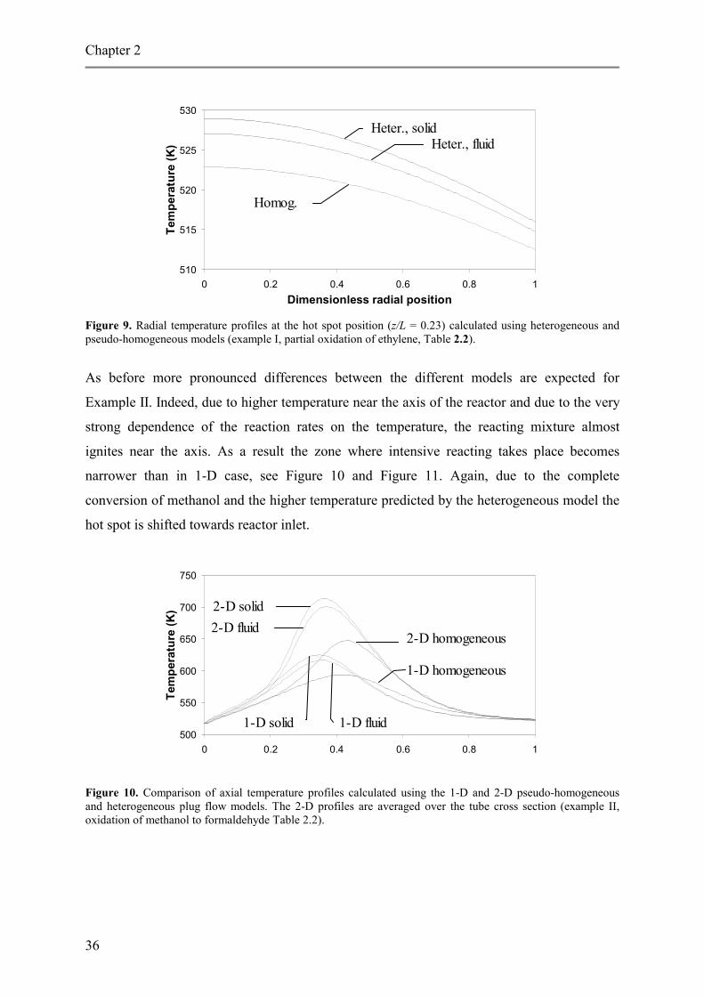
Figure 9. Radial temperature profiles at the hot spot position (z/L = 0.23) calculated using heterogeneous and pseudo-homogeneous models (example I, partial oxidation of ethylene, Table 2.2).

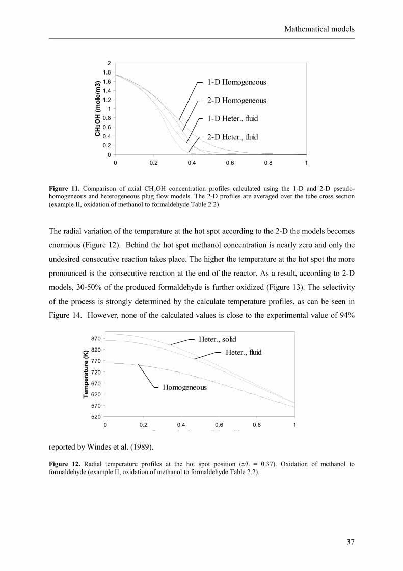
As before more pronounced differences between the different models are expected for

Example II. Indeed, due to higher temperature near the axis of the reactor and due to the very

strong dependence of the reaction rates on the temperature, the reacting mixture almost

ignites near the axis. As a result the zone where intensive reacting takes place becomes

narrower than in 1-D case, see Figure 10 and Figure 11. Again, due to the complete

conversion of methanol and the higher temperature predicted by the heterogeneous model the

hot spot is shifted towards reactor inlet.

Figure 10. Comparison of axial temperature profiles calculated using the 1-D and 2-D pseudo-homogeneous and heterogeneous plug flow models. The 2-D profiles are averaged over the tube cross section (example II, oxidation of methanol to formaldehyde Table 2.2).

510

515

520

525

530


Tem

pera

ture

(K)

Heter., solidHeter., fluid

Homog.

500

550

600

650

700

750

0 0.2 0.4 0.6 0.8 1Demensionless axial position

Tem

pera

ture

(K) 2-D solid

2-D fluid2-D homogeneous

1-D homogeneous

1-D fluid1-D solid

Mathematical models

37

Figure 11. Comparison of axial CH3OH concentration profiles calculated using the 1-D and 2-D pseudo-homogeneous and heterogeneous plug flow models. The 2-D profiles are averaged over the tube cross section (example II, oxidation of methanol to formaldehyde Table 2.2).

The radial variation of the temperature at the hot spot according to the 2-D the models becomes

enormous (Figure 12). Behind the hot spot methanol concentration is nearly zero and only the

undesired consecutive reaction takes place. The higher the temperature at the hot spot the more

pronounced is the consecutive reaction at the end of the reactor. As a result, according to 2-D

models, 30-50% of the produced formaldehyde is further oxidized (Figure 13). The selectivity

of the process is strongly determined by the calculate temperature profiles, as can be seen in

Figure 14. However, none of the calculated values is close to the experimental value of 94%

reported by Windes et al. (1989).

Figure 12. Radial temperature profiles at the hot spot position (z/L = 0.37). Oxidation of methanol to formaldehyde (example II, oxidation of methanol to formaldehyde Table 2.2).

00.20.40.60.8

11.21.41.61.8

2

0 0.2 0.4 0.6 0.8 1Demensionless axial position

CH

3OH

(mol

e/m

3) 1-D Homogeneous

2-D Homogeneous

1-D Heter., fluid

2-D Heter., fluid

520

570

620

670

720

770

820

870

0 0.2 0.4 0.6 0.8 1Demensionless radial position

Tem

pera

ture

(K)

Heter., solid

Heter., fluid

Homogeneous

Chapter 2

38

Figure 13. Comparison of axial CH2O concentration profiles calculated using the 1-D and 2-D, pseudo-homogeneous and heterogeneous plug flow models. The 2-D profiles are averaged over the tube cross section (example II, oxidation of methanol to formaldehyde Table 2.2).

Figure 14. Formaldehyde selectivity calculated using the 1-D and 2-D, pseudo-homogeneous and heterogeneous plug flow models (Example II, Table 2.2).

Summarizing the comparison of model performances for the two considered systems, it is

concluded that for the first reaction system (ethylene partial oxidation) with moderate heat

generation and smooth temperature and concentration variations in the reactor all the models

predict almost identical results. However, the predictions by the different models for the

second reaction system (methanol partial oxidation) fail to agree with each other.

Taking radial non-uniformities and/or temperature and concentration differences between the

bulk of the fluid and the catalyst surface into account result in higher hot spot temperature

and lower product selectivities. Finally, it is worth noting that the authors of the methanol

oxidation experiments (Example II, Windes et al., 1989) were able to fit the data obtained

from their pilot plant reactor only by varying some of the heat transfer parameters, e.g.

0

0.2

0.4

0.6

0.8

1

Sele

ctiv

ity

1-D, Homog

1-D, Hetero

2-D, Homog

2-D, Hetero

0

0.2

0.4

0.6

0.8

1

1.2

1.4

1.6

0 0.2 0.4 0.6 0.8 1Demensionless radial position

Tem

pera

ture

(K)

2-D Homogeneous

2-D Heter., fluid

1-D Homogeneous 1-D Heter., fluid

Mathematical models

39

assuming a Peclet number dependent on the temperature. These discrepancies will be

discussed in more detail in Chapter 5.

2.2.6 Models accounting for intraparticle resistance. The effectiveness factor

All the models described above neglect the resistance to heat and mass transfer inside the

catalyst particle. This is only rigorous if catalytically active components are deposited on the

outer surface of the catalyst pellets. The majority of catalysts have, however, a porous

structure, where most of the catalytically active surface resides on the interior surface which

can only be accessed via the pores. In a porous catalyst the reaction takes place

simultaneously with heat and mass transport and both processes must usually be considered

together. A one-dimensional pseudo-homogeneous plug flow model accounting for both

interface and intraparticle resistances for simple shape particles reads:

( )( ) ( )

,

,4

i

s sis f v i

s sws f p w fs v

dCu k a C Cdz

dT Uu c T T h a T Tdz dt

ρ

= −

= − + − (2.19)

( , )

( , )

sep p s si

ip

sep p s s

Tp

D C R C T

T R C T

ξξ ξ ξλ

ξξ ξ ξ

∂ ∂ = −∂ ∂

∂ ∂ =∂ ∂

(2.20)

with the accompanying boundary conditions

( ) ( )

0 00 : ,

0 : 0, 0

: ,2

i isi

s sp s si

ep f i i ep fs

z C C T TC T

d C TD k C C h T T

ξξ ξ

ξ λξ ξ

= = =

∂ ∂= = =∂ ∂

∂ ∂= − = − − = −∂ ∂

(2.21)

where ξ denotes the position inside the particle; p = 0, 1, 2 for a slab, an infinite cylinder and

a sphere respectively.

Equations (2.20) and (2.21) form the single particle problem with Robin’s type boundary

conditions. If temperature and concentrations on the particle surface are kept constant then

(2.21) must be replaced by

Chapter 2

40

0 : 0, 0

: ,2

si

p s si i

C T

dC C T T

ξξ ξ

ξ

∂ ∂= = =∂ ∂

= = = (2.22)

(2.20) and (2.22) define the single particle problem with Dirichlet type boundary conditions.

Incorporation of intraparticle resistances into an overall reactor model adds an additional –

the intraparticle – dimension into the problem. Generally, due to the non-linearity of the

reaction rates and the coupling between several mass and energy conservation equations, the

single particle problem can only be solved numerically. This considerably complicates the

handling of the differential equations. To avoid this complication the idea of the effectiveness

factor was introduced independently by Thiele (1939) and Zeldowitsch (1939). The

effectiveness factor is defined as the ratio of the reaction rate taking transport limitations into

account to the reaction rate without transport limitations (i.e. at particle surface conditions).

reaction rate with transport limitationsreaction rate without transport limitations

η =

Extensive investigation of analytical solutions and methods for the approximation of the

effectiveness factor can be found in Aris (1975a,b) and Wijngaarden et al. (1998). The

effectiveness factor can be calculated analytically for a first order reaction in an isothermal

simple shape particle.

For a slab:

φφη tanh= (2.23)

for an infinite cylinder:

)2()2(

0

1

φφφη

II= (2.24)

for a sphere:

231)3coth(3

φφφη −= (2.25)

Here

R(C,T) = kC (2.26)

Mathematical models

41

and p

p ep

V kA D

φ = is the Thiele modulus.

For non-linear reaction rates and arbitrary particle shapes analytical expressions for the

effectiveness factor do not exist. Its approximation for arbitrary kinetics and particle shape

can be calculated employing equations (2.23)-(2.25) using the generalized Thiele modulus , 1/ 2, ,

,

0

( , ) ( , )2

s ss s s s Cp s s s s

p ep

V R C T R C T dCA D

φ−

= ∫

This approach gives satisfactory results if φ is sufficiently large and chemical reaction occurs

only in the thin layer near the outer catalyst surface, so that η differs significantly from 1. In

opposite case of small φ, when η → 1, the shape of the catalytic particles becomes an

important factor influencing the value of the effectiveness factor. A new approach for the

calculation of the effectiveness factor for a particle of arbitrary shape and for arbitrary

reaction rates has recently been proposed by Wijngaarden et al. (1998). The authors introduce

two new dimensionless groups:

zeroth Aris number

( ) ( ),2 2 , ,

,0

0

,,

2

s ss s s s Cp s s s s

p ep

R C TVAn R C T dC

A D

=

∫

and first Aris number

( ),

2 ,

1

,

s s s

s s sp

sp ep

C C

R C TVAn

A D C=

∂ Γ= ∂

where Γ is the geometry factor, depending only on the shape of the pellet. In particular, Γ =

2/3, 1, 6/5 for a slab, an infinite cylinder and a sphere, respectively. The zeroth Aris number

is designed for the calculations of the effectiveness factor in the low η region; 0An is just

the well known Thiele modulus. The first Aris number determines the effectiveness factor

when its value approaches 1. The two asymptotic expressions are combined into a

generalized equation

0 1

11 (1 )An An

ηη η

=+ − +

which can be solved, e.g. by an iterative procedure. The details of the derivation along with a

discussion about the capabilities of the approach are given in Wijngaarden et al. (1998).

The concept of the effectiveness factor makes it possible to replace (2.20) and (2.21) by

Chapter 2

42

525

526

527

528

529

530

0 0.2 0.4 0.6 0.8 1

Dimensionless radial position

Tem

pera

ture

(K)

0.6

0.65

0.7

0.75

0.8

0.85

0.9

0 0.2 0.4 0.6 0.8 1


Dim

ensi

onle

ss

conc

entr

atio

n

( )( ) ),(

),(ss

Tsvf

ssii

svf

TCRTTah

TCRCCaki

η

η

=−

−=− (2.27)

Figure 15 - Figure 20 show axial temperature profiles calculated by: the complete model

(2.19)-(2.22) accounting for intraparticle heat and mass transport; the model with the

effectiveness factor and the model neglecting the intraparticle transport limitations.

Calculations were carried out for Example I using data given in Table 2.2). To allow

comparison of calculated and analytical solutions, the first reaction was ignored, i.e. R1 = 0.

To elucidate the significance of different factors the original parameters were varied. The rate

of the second reaction was slightly modified 2 2 O2=α 2430K CR ⋅ . α = 1.2 for the calculations

presented in Figure 15 - Figure 17 and α = 1.0 for the calculations Figure 18 – Figure 20. To

avoid temperature profiles inside the pellet the effective thermal conductivity inside the

particle was set to a large value of 10 W/m/K, Figure 15- Figure 17. Furthermore, to

emphasize diffusion limitations, see Figure 15 and Figure 18, the effective diffusivity inside

the particle Dep was decreased to 10-6 m2/s. The radial temperature and concentration profiles

inside the catalyst particle are given at the axial position of the hot spot, where the

effectiveness factor reaches its minimum.

Figure 15. Temperature and concentration profiles inside the spherical pellet (z/L = 0.2).

Mathematical models

43

Figure 16. Axial temperature profiles calculated using: I – the complete model (2.19)-(2.21), II – approximate model (2.19), (2.27) with the effectiveness factor η calculated by (2.25), III - solution to (2.19), (2.27) calculated neglecting intraparticle resistances, i.e. η = 1.

Figure 16 shows that intraparticle diffusion resistance reduces the reaction rate and as a result

the temperature at the hot spot is decreased – maximum temperature rise in the reactor is

reduced by a factor of 2. Figure 17 demonstrates that virtually identical results are obtained

using the effectiveness factor and by numerical solution of the single particle problem.

Figure 17. The effectiveness factor along the reactor: I) calculated by numerical solution of the single particle problem; II) calculated approximately using (2.25). Isothermal particle.

For the realistic value of the effective particle thermal conductivity λep of 0.12 W/m/K the

pellet is no longer isothermal. For the same effective diffusivity Dep of 10-6 m2/s the diffusion

limitations are also present, see Figure 18.

0.8

0.85

0.9

0.95

1

0 0.2 0.4 0.6 0.8 1

Dimensionless axial position

Effe

ctiv

enes

s fa

ctor

, η

I

II

500

510

520

530

540

550

0 0.2 0.4 0.6 0.8 1

Dшmensionless axial position

Tem

pera

ture

(K)

III

I, II

Chapter 2

44

524526528530532534536538540


Tem

pera

ture

(K)

0.6

0.7

0.8

0.9

1


Dim

ensi

onle

ss

conc

entr

atio

n

Figure 18. Temperature and concentration profiles inside the spherical pellet (z/L =0.2).

As a result of the “competition” between heat and mass transport in the particle the

effectiveness factor may exceed one. It was shown by Weisz and Hicks (1962) that the

effectiveness factor can be much grater than unity. In Figure 20 it is clearly shown that

disregard to intraparticle profiles may lead to significant underestimation of the maximum

temperature in the reactor.

Figure 19. The effectiveness factor along the reactor calculated by numerical solution of the single particle problem. Non-isothermal particle.

Figure 20. Axial temperature profiles calculated using: I – the complete model (2.19)-(2.21), II - solution to (2.19), (2.27) calculated neglecting intraparticle resistances, i.e. η = 1.

1

1.05

1.1

1.15

0 0.2 0.4 0.6 0.8 1

Demensionless axial position

Tem

pera

ture

(K)


505

510

515

520

525

530

0 0.2 0.4 0.6 0.8 1


Tem

pera

ture

(K)

Mathematical models

45

Finally, it is worth noting that in most practical applications catalyst particles are usually

principally isothermal and only external heat transport limitations play a role, whereas

resistance to mass transfer inside the particle usually dominates over the interfacial mass

transfer resistance.

2.2.7 Models accounting for the radial porosity distribution

Classical continuum models can be extended by accounting for the radial porosity

distribution in the packed bed. It was shown by many authors, a.o. by Benenati and Brosilow

(1962), Ridgway and Tarbuck (1966) and Goodling et al. (1986), that the void fraction varies

over the cross section of the reactor. The void fraction for a packed bed filled with spheres

decreases in a strongly damped oscillatory way from 1 at the wall to

Figure 21. Void fraction distribution across packed bed.

about 0.38 at the distance of 3-4 particle diameters from the wall, see Figure 21. For a packed

bed filled with cylindrical particles the value of porosity approaches 0.25 at about the same

distance from the wall. The oscillatory behavior is caused by the higher degree of particle

rdp

1

0.5

cylinders

spheres

ε

Chapter 2

46

ordering near the wall. As a result the layer adjacent to the wall is nearly free of catalyst,

whereas at a distance of a half particle diameter from the wall the catalyst fraction is

maximal.

Many authors, a.o. Schwatz and Smith (1953), Schertz and Bishoff (1969) and Marvioet et al.

(1974) experimentally observed that the drop in porosity near the wall leads to channeling

effects. Variations in the velocity profile were also calculated from the pressure drop

equation. Foscolo et al. (1983) modified the Ergun equation (2.2), (2.3) so that the pressure

drop equation accounts for the radial porosity distribution.

A more accurate approximation of the velocity profile was obtained by Vortmeyer and

Schuster (1984). Following Brinkman (1947) they accounted for the viscous friction inside

the fluid itself in addition to the interaction of the fluid with the particles. Superimposing the

viscous term to the Ergun equation and introducing a no-slip boundary condition Vortmeyer

and Schuster (1984) derived an expression for the the radial velocity profile. A typical radial

velocity profile is shown in Figure 22.

Figure 22. Typical dimensionless radial velocity profile in a packed bed; dt/dp = 9, Re = 600; u0 is averaged velocity.

Incorporation of radial porosity and velocity profiles in a 2-D model transforms the set of

model equations given by (2.16) into

0

0.5

1

1.5

2

0 0.2 0.4 0.6 0.8 1


u/u0

Mathematical models

47

( ) ( ) ( )

( ) ( ) ( )

11 ( , )111 ( , )

1

i is er i

s f p er T

rC Cu r D r r R C Tz r r r

rT Tu r c r r R C Tz r r r

εεε

ρ λε

−∂ ∂ ∂ − = − ∂ ∂ ∂ −

−∂ ∂ ∂ − = ∂ ∂ ∂ −

(2.28)

The difference between this extended model and the classical continuum model (2.16) boils

down to: differences in residence time distributions variation of the catalyst density in the bed

and modified heat and mass transport parameters. Based on these effects Delmas and

Froment (1988) and Vortmeyer and Haidegger (1991), discriminated several approaches to

incorporate radial porosity and velocity profiles. In the latter a good description of the

experimental data was obtained even when neglecting the influence of the porosity

distribution on the radial heat and mass transfer coefficients. Calculation of dispersion

coefficients Der and λer as functions of the radial position is somewhat speculative, since the

dependence on the radial velocity profile u(r) is not clear. Delmas and Froment (1988)

performed several calculations using the extended model (2.28) and manipulating the

transport coefficients. The wall-to-bed heat transfer coefficient hw was omitted in the

boundary conditions and the resistance to heat transfer to the wall was incorporated by

decreasing λer near the wall. Heat and mass dispersion coefficients Der and λer were supposed

to be proportional to: a) the velocity u(r), b) catalyst fraction (1 - ε(r)) and c) both u(r) and

(1-ε(r)). Different temperature and concentration profiles were calculated depending on the

adopted assumption. The dependence of the transport parameters on the radial position is still

a subject of discussions.

Generalization of (2.28) to models including axial dispersion effects and/or to heterogeneous

models is straightforward.

2.2.8 Dynamic models Along with the steady state, the dynamic modeling of packed bed reactors has attracted

considerable attention. Interest in dynamic modeling can be explained by the necessity to

study important practical problems such as: 1) dynamically operating reactor, e.g. reverse

flow reactors; 2) reactor start-up and shut down; 3) process stability, i.e. response of the

reactor to disturbances in operation condition.

Chapter 2

48

Equations of the dynamic models are typically the same as for steady state models, only

additional terms describing the rates of temperature and concentrations change in time i.e.

Tt

∂∂

, Ct

∂∂

, sT

t∂∂

and sC

t∂∂

are added.

During investigation of the abovementioned problems several, somewhat confusing, effects

were predicted analytically and observed experimentally: multiplicity of steady-state

solutions, wrong-way transient behavior and creeping reaction fronts.

There are two physical phenomena responsible for multiplicity. It has been shown by a.o.

Hlavacek and Hoffman (1970), Varma and Amundson (1972, 1973a, 1973b) and Puszynski

et al. (1981) that the dispersion effect is the underlying mechanism of multiplicity. Using

pseudo-homogeneous models with axial dispersion they where able to predict a number of

steady states for different systems. According to Sharma and Hughes (1979) a two phase

model was required to accurately model their experimental data for the same reaction system.

Interfacial heat and mass transfer resistance constitutes the second effect, which can lead to

multiplicity. It was shown by Liu and Amundson (1962) that an infinite number of steady

states may exist in certain parameter regions. This approach claims that if any particle in the

bed has multiple steady states then the system will be unstable in a certain range of initial

conditions. In that range the occurrence of even a slight heat transport between particles is

sufficient to shift the particle from one steady state to another. As a result, non-unique

solutions for the packed bed can be obtained. It was shown by Eigenberger (1972a,b) that

incorporation of thermal conduction through the solid phase reduces the infinite number of

steady states to only a few. The main mechanism of heat exchange between adjacent particles

is usually the heat transfer via the fluid in between the particles. Radiation also contributes to

the effective solid conductivity. Existence of multiple (twofold) steady states was

experimentally proven by Hlavacek and Vortuba (1974) and Sharma and Hughes (1979) in

their studies on carbon monoxide oxidation.

The second perplexing phenomenon observed during the dynamic operation of packed bed

reactors is the so-called wrong-way behavior. Wrong-way behavior refers to the process of

transient reactor temperature rise in response to a decrease in the feed temperature. It was

first predicted by Boreskov and Slinko (1965). In contrast to multiplicity, wrong-way

behavior is predicted even by the simplest pseudo-homogeneous plug-flow model (Mehta et

al., 1981). The phenomenon is associated with a difference in propagation speed for thermal

and concentration disturbances. A colder feed cools the inlet section of the reactor and

Mathematical models

49

decreases the reaction rate and conversion. The cold fluid with high concentration of reactant

eventually reaches the hot catalytic particles in the downstream section of the bed, where the

reaction rate very rapidly increases. This causes a transient temperature rise. Wrong-way

behavior was observed experimentally and modeled mathematically by Van Doesburg and

De Jong (1974). Incorporation of thermal dispersion into the model decreases the magnitude

of the transient temperature excursion (Panjala et al., 1988), but also introduces phenomenon

of possible multiple steady states. Wrong-way behavior occurring in the region of

multiplicity was experimentally observed by Sharma and Hughes (1979).

Finally, the third interesting experimentally observed phenomenon is the formation of very

steep reaction fronts moving with nearly constant velocity without significant changes in their

shape (Vortmeyer and Janhel, 1972; Kalthoff and Vortmeyer, 1980). The velocity of the

reaction wave (creeping fronts) is controlled by the feed conditions as well as by the flow

velocity. Depending on these conditions, the reaction front moves downstream, upstream or

rests at certain position. The width of the reaction front – area where most of the reaction

takes place – can be as narrow as 2-3 particle diameters. Observed experimental results were

mathematically described by the authors using a 2-D pseudo-homogeneous model with axial

dispersion and radial porosity and velocity distributions.

2.3 Cell models

Next to continuum models, cell models are used to describe the physical-chemical

phenomena in packed bed reactors. A cell model was first proposed by Deans and Lapidus

(1960). In the cell models the reactor is represented by a network of ideally stirred tank

reactors (cells). Each cell is defined as a part of the reactor confined by two coaxial

cylindrical surfaces and two planes perpendicular to the reactor axis, as illustrated by the

shaded volume in Figure 23. The number of parallel planes intersecting the reactor, N,

defines the number of stages. The number of imbedded cylinders, M, defines the number of

cells over the cross-section of the reactor. Mixing effects in the network are determined by N

and M. If N is taken equal to the number of particles along the reactor, the axial Peclet

number is equal to 2.

Chapter 2

50

Figure 23. Schematic representation of a single cell, used as a building block in the cell models.

The simplest cell model is obtained by assuming that the network is a one-dimensional series

of stirred tanks:

where each tank represents one stage of the reactor. The model is equivalent to the finite-

difference approximation of the one-dimensional pseudo-homogeneous continuum model.

Mixing effects can be enhanced by introducing additional interactions between the cells. Also

heterogeneity can also be easily incorporated into the cell model:

This scheme corresponds to the one-dimensional heterogeneous model with axial dispersion.

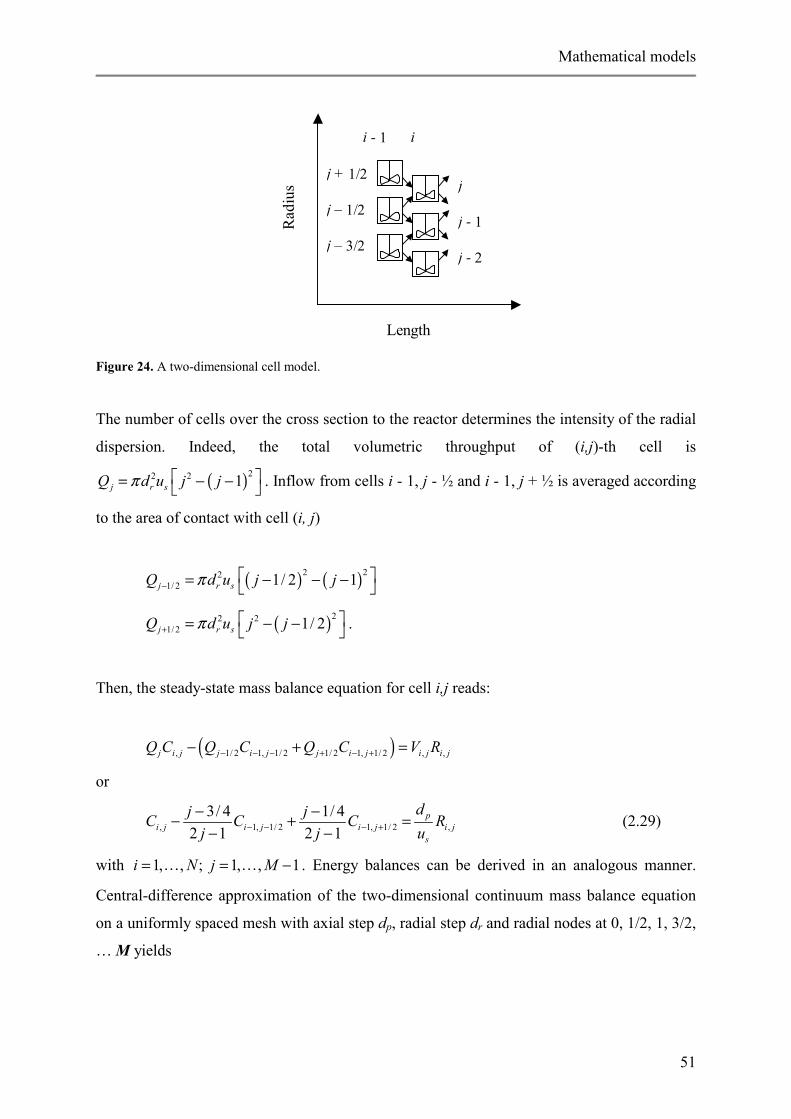
Two-dimensional cell models are defined by two-dimensional arrays of ideally stirred tanks.

Each cell at level i is influenced by two neighboring cells from level i-1, as indicated in

Figure 24.

fluid phase

solid phase

Mathematical models

51

Figure 24. A two-dimensional cell model.

The number of cells over the cross section to the reactor determines the intensity of the radial

dispersion. Indeed, the total volumetric throughput of (i,j)-th cell is

( )22 2 1j r sQ d u j jπ = − −

. Inflow from cells i - 1, j - ½ and i - 1, j + ½ is averaged according

to the area of contact with cell (i, j)

( ) ( )2 221/ 2 1/ 2 1j r sQ d u j jπ−

= − − −

( )22 21/ 2 1/ 2j r sQ d u j jπ+

= − −

.

Then, the steady-state mass balance equation for cell i,j reads:

( ), 1/ 2 1, 1/ 2 1/ 2 1, 1/ 2 , ,j i j j i j j i j i j i jQ C Q C Q C V R− − − + − +− + =

or

, 1, 1/ 2 1, 1/ 2 ,3/ 4 1/ 4

2 1 2 1p

i j i j i j i js

dj jC C C Rj j u− − − +− −− + =− −

(2.29)

with 1, , ; 1, , 1i N j M= = −… … . Energy balances can be derived in an analogous manner.

Central-difference approximation of the two-dimensional continuum mass balance equation

on a uniformly spaced mesh with axial step dp, radial step dr and radial nodes at 0, 1/2, 1, 3/2,

… M yields

ii - 1

j

j - 1

j - 2j – 3/2

j – 1/2

Rad

ius

Length

j + 1/2

Chapter 2

52

1, 1/ 2 1, 1/ 2, 1, 1, 1/ 2 1, 1, 1/ 2 ,2 2

2p er i j i j p

i j i j i j i j i j i js r s

d D C C dC C C C C R

u d j u− + − −

− − + − − −

− − − − + + =

(2.30)

1, , ; 1, , 1i N j M= = −… …

It can be seen that equation. (2.29) approximates (2.30) with an accuracy O(dr), if

2

21p er

s r

d Du d

= . In other words, if the number of cells M is set equal to / 8t mrd Pe then equation

(2.29) also approximates the corresponding continuum model. The effective radial dispersion

coefficient in continuum models is proportional to the square of the cell size. In addition, the

larger the value of M the closer the solutions of (2.29) and (2.30). Similar considerations

show that each cell model has its analogue in the family of finite-difference approximations

of continuum models. Consequently, the classification of continuum models can be extended

to the cell models.

The numerical treatment of the cell models can be easier than that of continuum models. The

number of algebraic equations making up a cell model is generally smaller than that resulting

from finite-difference approximations of continuum models. In addition, some cell models

allow a marching technique for their solution, as for example, for equation (2.29). The

diffusion terms in the continuum models are usually treated implicitly which results in a large

number of algebraic equations that must be solved simultaneously.

Despite of these, the cell model equations retain the main problems typical for finite-different

approximations of continuum models and require similar effort to calculate their solution.

2.4 Summary and conclusions

Several types of mathematical models approximating complex physical-chemical processes

taking place in packed bed catalytic reactors are considered. Of all the considered models

(continuum, channel, cell) the continuum models are most widely used and have been

systematically investigated in this chapter. Predictions of the different continuum models

were compared based on two industrially important processes: oxidation of ethylene and

oxidation of methanol to formaldehyde. The first process considered at chosen operating

conditions is a moderately energetic with relatively smooth temperature and concentration

profiles in the reactor. Maximal temperature rise reached in the reactor is about 20-40oC. The

second process represents a very exothermic system. Temperature rise in the reactor is 150-

Mathematical models

53

200oC. The temperature variation in the radial direction can be higher than 100oC at the hot

spot position.

It has been shown that temperature and concentration profiles predicted by different models

for the ethylene oxidation process are not very sensitive to the chosen model. Estimated

difference between predictions of one-dimensional pseudo-homogeneous and one-

dimensional heterogeneous model is about 5%. The difference between the 1-D and 2-D

models is even less.

The second system demonstrated a huge discrepancy between the predictions of different

models. Many processes taking place in the reactor cannot be lumped together and should be

considered explicitly. The difference between the temperature of the solid phase and the bulk

fluid temperature can be about 10oC. This results in large discrepancy between the predictions

of the pseudo-homogeneous and the heterogeneous models. The estimated difference in heat

production is is more than 15%. Due to pronounced radial temperature and concentration

profiles the two-dimensional models are preferred to one-dimensional models. In addition, the

diffusion limitations in the catalytic particle have significant effect on the model predictions.

Therefore the concept of the effectiveness factor was incorporated. Despite of such detailed

modeling the considered mathematical models failed to explain experimental reactor behavior

observed by Schwedock et al. (1989). Although there is always a possibility of experimental

errors and in the data used in the models (especially in the reaction rate expression), the

inconsistencies are so systematic that the possibility of existence of model shortcomings

becomes significant. Other experimental data on intensive processes in packed bed reactors

(Hoffman, 1979; Clement and Jørgensen, 1983) also show significant discrepancies between

the standard dispersion models predictions and the experimental evidence. The trustworthiness

of standard dispersion models is even more uncertain since they do not have rigorous

mathematical derivation or a proper physical justification. Furthermore, the models contradict

to physical reality. For example, they assume infinite speed of signal propagation and as a

consequence allow backmixing; whereas, in real packed bed reactors signals propagate with

finite speed and usually no backmixing is observed (Hiby, 1962 and Benneker et al., 2002).

To overcome some of the conceptual shortcomings of the mentioned dispersion models the

wave models will be considered in chapter 5. The concept of heat and mass transport by waves

has been introduced by Westerterp et al. (1996) and Kronberg et al. (1999) and avoids such

Chapter 2

54

inherent drawbacks of the standard dispersion models as infinite speed signal propagation,

backmixing and the necessity of outlet boundary conditions.

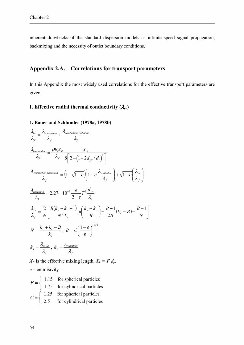
Appendix 2.A. – Correlations for transport parameters

In this Appendix the most widely used correlations for the effective transport parameters are

given.

I. Effective radial thermal conductivity (λλλλer)

1. Bauer and Schlunder (1978a, 1978b)

,conduction radiationer convection

f f f

λλ λλ λ λ

= +

( )28 2 1 2 /

s pconvection F

f f pv t

u c X

d d

ρλλ λ

= − −

( )

−+

+−−=

f

rs

f

radiation

f

radiationconduction

λλε

λλεε

λλ

1111,

7 32.27 102

pvradiation

f f

de Te

λλ λ

−= ⋅−

( ) ( )

−−−++

+−+=

NBBk

BB

Bkk

kNkkB

N rrs

s

rs

f

rs 12

1ln12

2λλ

s

rs

kBkkN −+= ,

9/101

−=εεCB

f

solidsk

λλ= ,

f

radiationrk

λλ=

XF is the effective mixing length, XF = F dpv

e – emmisivity

1.15 for spherical particles 1.75 for cylindrical particles

F =


C =

Mathematical models

55

2. Dixon and Cresswell (1979) and Dixon (1988) 1/ 4 41 1 8

Re Prrs f f s

er fr f s s

Bi BiPe Pe Bi N Bi

λ λ − + += + +

(Re > 50)

14 /41 1 8

Re Prf rs fs

er fr s F f

BiBiPe Pe Bi N Bi

λ λ−

+ += + +

(Re < 50)

1 1 0.74( ) Re Prrf rfPe Pe

ε= +∞

( )cylindershollow

cylindersspheres

Perf

=∞67

12

( )

−−+−

−−=

MBB

Bk

kMkB

Ms

s

s

f

rs 12

1ln121 2ε

λλ

s

s

kBkM −=

f

solidsk

λλ=

9/101

−=εεCB

( ) ( )( )PrRe/2/ rfpvtwff PeddNuBi = 6.03/1 RePr1.10.2 +=fsNu

( ) 738.033.0 RePr/1523.0 tpvwf ddNu −= (2.31)

( )( )

2

2

2.41 0.156 / 1

0.48 0.192 / 1

t pvs

t pv

d d spheresBi

cylindersd d

+ −= + −

s

s

s

frss

BiBi

N48

/+

+=

λλβ ,

f

f

s

rfs

BiBi

N

Pe48

Pr/Re+

+=β ,

+

−=

solid

f

fsf

rs

pv

t

p

p

s

Nu

dd

VA

N

λλ

βλλ

ε

11

)1(25.02

,

+

−=

solid

f

fsrf

pv

t

p

p

F

NuPe

dd

VA

N

λλ

β

ε

11PrRe

)1(25.02

=particlelcylindrica

particlespherical8

10β

Chapter 2

56


C =

(2.31) is taken from Colledge and Paterson (1984)

3.Specchia et al. (1980)

er convection conduction

f f f

λ λ λλ λ λ

= +

Re Prconvection a

f Kλλ

= ,

solid

ff

conduction

λλ

γϕ

εβελ

λ

+

−+= )1(

+=

2

4.19165.8t

pa

dd

K , 222.0,3/2,1 εϕγβ ===

4.Yagi and Wakao (1959)

Pr Reer

f

λ α βλ

= +

For glass spheres and broken cement clinker:

α = 6

0.11, 0.021 / 0.0720.09, 0.12 / 0.17

p t

p t

d dd d

β< <

= < <

For metal spheres

α = 13, β = 0.11, 0.021 < dp/dt < 0.086

Other references:

VDI Wärmteatlas, 4th ed., VDI Vrelag GmbH, Dusseldorf, 1984

De Wasch, A. P. and Froment, G. F., Chem. Eng. Sci. 27, 567-576, 1972

Cybulski, A and Kawecki, W., Inz Chem 2(2), 355, 1972

Yagi, S., Kuni, D. and Wakao, N., Int. Dev. Heat Transfer, Proc. 1961-62. Heat transfer

Conf. Boulder Colorado, New York. 1963

Caldwell, A. D., Chem. Eng. Sci. 23(4), 393, 1968

Mathematical models

57

II Effective radial diffusivity (Der)

1. Bauer and Schlunder(1978)

( )[ ]2/2128 tpv

ser dd

XuD F

−−=

XF – effective mixing length, XF = F dpv


F =

2. Rase, H. F., (1990)

For dpa/dt > 0.1 1 0.38Re

er

s pa

Du d mε = +

For dpa/dt < 0.1 divide Der calculated from above by

+

2

4.191t

pa

dd

11 Re>40057.85 - 35.36 logRe + 6.68 (logRe)2 20<Re<400

m =

3. Specchia et al. (1980)

2

8.65 1 19.4

s paer

pa

t

u dD

dd

= +

Other references:

Brenard, R. A. and Wilhelm, R. H., Chem. Eng. Prog., 46, 233, 1950

Wen, C. Y. and Fan, L. T., Models for flow systems and chemical reactors, Dekker, New

York, 1975

Fahien, R. W. and Smith, J. M. AIChe J., 1 25, 1955

Froment, G. F., Ind. Eng. Chem. 59, 27, 1967

Chapter 2

58

III Wall heat transfer coefficient (hw)

1. Dixon (1988)

8 1/ Re Pr

w pv rfsw fw s

f t pv pv

h d PeNu Nu

d dβ β

λ

= = + +

, Re > 50

82 1

/ /w pv f pv frs

w sf t pv t rs f

h d dNu Bi

d d f dβ βλ

λ λ λ λ

= = + +

, Re < 50

The definitions of βs, βf,, λrs, Bis and Perf are given in correlation 2 for effective radial

conductivity.

2. Li and Finlayson (1977)

Spherical particle, 0.05 < dh/dt < 0.3, 20 < Reh < 7600:

h

pvh

f

pvww d

ddhNu 33.079.0 PrRe19.0==

λ

Cylindrical particle, 20 < Reh < 800, 0.03 < dh/dt < 0.2:

h

pvh

f

pvww d

ddhNu 33.093.0 PrRe18.0==

λ

3. Specchia et al. (1980)

( ) ( )conductionwconvectionww hhh +=

( )pa

fconvectionw d

hλ3/191.0 PrRe0835.0= , 10 < Re < 1200

( )pa

fconvectionw d

hλ3/153.0 PrRe23.1= , 1200 < Re < 10000

( )pv

f

wsolid

fw

conductionw dh

λ

ϕλλ

γ

εε

+

−+= 12

( )pvtww dd /0024.0,3/1 == ϕγ

Other references:

Yagi, S and Wakao, N., AIChE J. 5(1), 79-85, 1959

Mathematical models

59

Beek, J., Adv. Chem. Eng. 3, 203, 1962

Dixon, A. G., Paterson, W. R. and Cresswell, D. L. ACS Symp.Ser., 65, 238, 1978

Paterson, W. R. and Carberry, J. J., Chem. Eng. Sci. 18(1), 175, 1983

IV Overall heat transfer coefficient for 1-D model (Uw)

1. Dixon (1988)

43

611

+++=

BiBid

hU er

t

ww λ

( ) 0.33 0.7380.523 1 / Pr Refw pv t pvNu d d= −

++==

PrRe1

/8

pv

rfswf

pvt

s

f

pvww

PeNu

dddh

Nu ββλ

, Re > 50

++==

frs

f

t

pvrss

pvt

f

f

pvww d

df

Bidd

dhNu

λλβ

λλβ

λ /12

/8

, Re < 50

PrRe2 pv

erw

pv

t PeNuddBi =

The definitions of βs, βf,, λrs, Bis and Perf are given in correlation 2 for effective radial

conductivity.

2. Li and Finlayson (1977)

Spherical particle, 0.05 < dh/dt < 0.3, 20 < Reh < 7600:

−=

t

hh

f

tw

dddU 6expPrRe26.2 33.08.0

λ

Cylindrical particle, 20 < Reh < 800, 0.03 < dh/dt < 0.2:

−=

t

hh

f

tw

dddU 6expPrRe40.1 33.095.0

λ

Other references:

De Wasch, A. P. and Froment, G. F., Chem. Eng. Sci. 27, 567-576, 1972

Leva, M., Chem. Eng. (N.Y.) 56, 115, 1949

Chan, B. K. G., and Lawther, K. R., Austr A.E.C. AAEC/TM (Rep), 389, 1967

Chapter 2

60

V Axial heat dispersion coefficient (λλλλez)

1. Yagi et al. (1960) 0

Re Prez ez

f f

λ λ δλ λ

= +

δ = 0.7 for steel balls, δ = 0.8 for glass beads. Other data on δ and 0ezλ are given in Yagi et al.

(1960).

2. Vortuba et al. (1972)

0

3

14.46 RePr1

RePr

ez ez

f fp

Cd

λ λλ λ

= + +

0.1 < Re < 1000, 0.23 < dp < 6.5 mm;

2. Dixon and Cresswell (1979)

( )2

/1 1

1 8RePr 14

as g

hz fz s

s s

k kPe Pe Bi

N Bi

= + + +

1 0.73 0.59.7RePr 1

RePrfzPe

ε= + +

as rsk k= , other data related to this correlation is given in correlations 2 for effective radial

dispersion coefficient

VI Axial mass dispersion coefficient (Dez)

1. Edwards, M. F. and Richardson (1968)

1 0.73 0.59.7ReSc 1ReSc

mzPeε

ε= +

+

0.008 < Re < 50, 0.0377 < dp < 0.6 cm

Mathematical models

61

2. Wen and Fan (1975)

1 0.3 0.53.8ReSc 1

ReSchzPe= +

+

0.008 < Re < 400, 0.28 < Sc < 2.2

3. Bischoff and Levenspiel (1962)

1 0.457.3ReSc 1

ReSchzPe

ετ

= ++

τ is the tortuosity factor

VII Solid-fluid heat transfer coefficient (hfs)

1. Gnielinski (1982) and Martin (1978)

33.05.0 PrRe2 cparticle FNu +=

Re /( )pa f f pa fu dρ εµ= , f

fpCλµ

=Pr

( )

−++= −

2

1.067.0

67.03.0

Re1Pr44.21PrRe0557.01664.0

c

cF

c

pvparticle d

dNuNu )]1(5.11[ ε−+=

0.26 < ε < 0.935, 0.6 < Pr < 10000, RepPr > 100

2. Bird et al. (1960)

( ) 3001/Re,PrRe)1(27.2 33.049.051.151.0 <−−= εψε hh

pvh d

dNu

( ) 3001/Re,PrRe)1(27.1 33.059.041.141.0 >−−= εψε hh

pvh d

dNu

Chapter 2

62

=particlelcylindrica

particlesperical91.01

ψ

f

hffh

duµρ

=Re , f

fpCλµ

=Pr , f

pvs dNu

λα

=

Cylindrical particle.

3. Wakao et al. (1979)

Spherical particles. 33.06.0 PrRe1.12 pNu +=

fpffp du µρ /Re = , f

fpCλµ

=Pr , f

ps dNu

λα

=

VIII Solid-fluid mass transfer coefficient (kf)

Correlations are the same as for solid-fluid heat transfer coefficient. Only Pr is replaced by Sc

and Nu is replaced by Sh.

CHAPTER 3

3. Numerical methods and the package of programs for packed

bed modeling

Equation Section 3

Chapter 3

64

Abstract

Several numerical problems specific for packed bed reactor model equations are addressed

in this chapter. The stiffness of the model equation is tackled by a simple but robust method

based on the Newton-Kantorovich procedure and accompanied with an automatic time

stepping mechanism. A new technique is proposed to automatically select a minimum

possible number of differential equations to solve by introduction of new dependent

variables. This significantly reduces the required computer resources and computational time

in case of a large number of components. To solve heterogeneous model equations a method

to decouple the fluid and solid balance equations is proposed. As a result the entire system of

equations is basically splitted into two smaller subsystems, which are solved subsequently.

Finally, an algorithm for solution of sparse linear algebraic equations resulting from the

discretization of diffusion-type terms is proposed. The technique is efficient and easy to

implement. All the methods described in this chapter are used to enhance the performance of

classical finite-difference methods and are employed in the software package for

mathematical modeling of packed bed reactors.

Numerical methods

65

3.1 Introduction One of the main criteria for the evaluation of any mathematical model is its mathematical

feasibility. On one side, a model must explicitly include as many relevant physical-chemical

processes as possible. On the other side, more detailed models involve more complicated

differential equations and, consequently, are computationally more demanding. Certainly,

first of all, the level of model detailedness is determined by the availability of accurate kinetic

expressions and model parameters. However, the applicability of the model can also be

limited by the difficulties associated with its mathematical handling.

Equations encountered in packed bed reactor modeling range from algebraic equations to

multidimensional partial differential equations. Only very few and very simple models permit

exact analytical solutions, therefore the focus is on the numerical treatment of the model

equations. Fortunately, similar types of equations are encountered in other areas of

mathematical physics and have been investigated. Nevertheless, systems considered in this

work possess many specific properties that must be taken into account in order to efficiently

solve the equations. A system of algebraic-differential equations describing physical and

chemical processes in the catalytic packed bed reactor is of the reaction-convection-diffusion

type and inherits all the numerical problems specific for this type of system. The most

important numerical problems are:

1. Large differences in characteristic times for different reactions (reaction stiffness)

and physical processes.

2. Large number of equations

3. Strong sparsity of matrices involved

4. Numerical diffusion introduced by convection approximations

5. Non-physical oscillations near steep gradients and discontinuities

6. Reasonably looking but fake solutions

7. Strongly coupled equations resulting from coupling between physical- chemical

processes

All these problems are addressed in the computational routines included in software package

“PackSim” – a package especially developed for mathematical modeling of packed bed

Chapter 3

66

reactors. The package includes most of the classical continuum models as well as novel wave

models. The core of the package is made of computational units solving certain types of

equations. The equations are solved by finite-difference methods. The computational units

are embedded in a user friendly visualized interface.

In the following section some of these numerical techniques are described. Firstly, section 3.2

deals with the problem of stiffness. It is explained why the trapezoidal rule accompanied with

a robust Newton-Kantorovich technique and a step size control method is well suited to solve

a stiff system of equations. Section 3.3 represents a new technique to optimize the usage of

computer resources and required simulation time. Section 3.4 presents a new technique for

efficient “decoupling” of solid and fluid phase equations. The proposed method enables an

efficient extension of algorithms for the solution of homogeneous systems to heterogeneous

systems. Finally, section 3.5 describes a method designed to solve linear algebraic equations

with sparse matrices resulting from the discretization of the diffusive terms. This chapter

mainly focuses on the solution of classical continuum models. A numerical method for the

solution of the wave model equations is developed and presented in chapter 4.

3.2 Stiffness

The first problem addressed in this chapter is the stiffness of the source terms. The stiffness

of chemical systems is caused by extreme differences in time scales of different reactions.

The ratio of the characteristic times of the fastest and the slowest reactions determines the

stiffness ratio of the problem. In chemical reaction systems the stiffness ratio can easily reach

a magnitude of 105 - 107.

Numerical problems caused by stiffness can be nicely illustrated with a simple famous

problem described by Gear (1971):

998 1998 , (0) 1

999 1999 , (0) 0u u v uv u v v′ = ⋅ + ⋅ =′ = − ⋅ − ⋅ =

(3.1)

The analytical solution of this problem is given by

Numerical methods

67

1000

1000

2 t t

t t

u e ev e e

− −

− −

= −

= − +

Obviously, from the analytical solution it can be easily concluded that the contribution of the

second terms is negligibly small compared to the first terms. However, if the system is solved

numerically, e.g. by an explicit Euler method

1 0

1 0

(998 1998 ), 1, 1,2,3,...( 999 1999 ), 0, 1,2,3,...

n n n n

n n n n

u u h u v u nv v h u v v n

+

+

= + ⋅ + ⋅ = =

= + − ⋅ − ⋅ = =

the integration step size h has to be chosen as h = min(1/λ1, 1/λ2), where λ1 = 1 and λ2 = 1000

are the eigenvalues of the system. This restriction is dictated by stability considerations. A

stability analysis shows that for the explicit Euler method the error of the approximation is

amplified by factor (1-hλ2)-1 at each step. Obviously, for h > 1/λ2 the solution is

deteriorating.

Generally, by the definition of Dahlquist (1963), a method is said to be A-stable, if all

numerical approximations tend to zero as n → ∞ when it is applied to the differential

equation y yλ′ = with a fixed step size h and a constant λ with a negative real part. Any

method designed to solve problems involving chemical reactions must be A-stable or very

close to it. Most widely used and often recommended methods for solution of stiff problems

are so-called BDF-multistep methods of Gear, 1971. These methods can have an order up to

6 and still be close to A-stable methods. Also the method developed by Bader and Deuflhard,

1983 was applied to problems of chemical kinetics with great success. Their method

employed a semi-implicit extrapolation technique, has a high approximation order and is also

close to A-stable.

Respecting all the merits of these and some other techniques proposed in the literature,

another method has been implemented in the package – second order one-step implicit

trapezium rule.

( ) ( )1 1 1, ,n n n n n ny y h f t y f t y+ + + = + + (3.2)

Chapter 3

68

The method was the subject of the famous work of Dahlquist, 1963, where he proved that any

multi-step method of order higher than two cannot be A-stable and that the implicit

trapezoidal rule is the A-stable method of order 2 with smallest approximation error

coefficient. This is the first, but not the main reason of our choice. Our own experience shows

that the aforementioned higher order methods work better when applied to a system of

ordinary differential equations (ODE). But in practice most of the mathematical problems are

at least two-dimensional or non-steady state and ODE solvers are employed to solve

equations resulting after spatial discretization of the original partial differential equations.

The approximation order of the spatial discretization is limited due to either computational

cost or problems associated with the boundary conditions. Thus, the high order of the time

discretization can be spoiled by the errors of the lower order spatial approximation. On the

other side, high order approximation of spatial derivatives usually require costly techniques

and, therefore, high order temporal discretization, which usually include repeated spatial

discretizations at different time levels, leads to significant increase of the computational time

and complicates the implementation of the algorithm. In addition, high order temporal

discretization also requires repeated evaluations of the source term and their Jacobi matrices

at each spatial computational grid point, which is also very costly. A numerical method

designed in Chapter 4 to solve the wave and the convection dominated diffusion type models

clearly demonstrates the necessity of incorporating a simple but sufficiently robust method to

solve ODEs resulting from PDE spatial discretizations.

To be capable of dealing with stiff differential equation systems, a numerical method must

incorporate an automatic control of the integration step size. Step size adjustment not only

optimizes the integration step sizes, but also guaranties a certain predetermined accuracy of

the solution. This is especially important for “black-box” type software, to which “PackSim”

belongs, where the program should adjust itself to solve problems of different complexity.

Powerful techniques have been developed for ordinary differential equations (ODE), see, e.g.

Moore and Petzold (1994) and Hosea and Shampine (1994). These methods are robust and

efficient for ODEs, but are not well suited for large multidimensional PDE systems. To solve

these systems several aspects must be taken into account simultaneously: strongly nonlinear

kinetics and, consequently, embedded Newton type iterations in each time step; discretization

of diffusion terms; special treatment of convection terms; restrictions on the time step

Numerical methods

69

imposed by Courant-Friedrichs-Lewy (1928, 1967) condition; necessity of spatial mesh

adaptation. All these reasons make the usage of complex step size control strategies virtually

impossible.

A simple, yet effective and robust technique was implemented in “PackSim”. The method

addresses two major concerns: convergence of the Newton iterations and control of accuracy.

Firstly, the step size dt is adjusted to make the Newton iterations converge in kmax ~ 5-10

steps. If after kmax steps the accuracy (of the solution of nonlinear algebraic equations) tol1 has

not been achieved then the current dt is multiplied by k- ~ 0.5-0.7. If the accuracy tol1 is

achieved after 1-3 steps, then dt is multiplied by k+ ~ 1.2-1.4. The solution y1(t0 + dt) is

calculated from known y0(t0) with the time step size dt. The second solution y2(t0 + dt) is

calculated from t0 by two consecutive time steps of length dt/2.

Usually Newton iterations for these two steps converge very rapidly and no additional

adjustment of dt is required. Though the convergence of the Newton iterations very often

indicates the overall accuracy of the solution, more strictly, it is only a measure of the

accuracy of the algebraic equations obtained by certain discretization of the differential

equations. However, E = |y2(t0 + dt) - y1(t0 + dt)|/yscal is a good indication of the accuracy of

the time discretization itself. Here yscal serves as a scaling factor. For the trapezoidal rule E =

O(dt3). In the proposed automatic time step size control E is made small enough by halving

dt, until the first k ~ 3-5 digits of y1 and y2 are coinciding. In this method only the calculations

for the first chosen dt0 can be somewhat time consuming, and for all the following integration

steps the intermediate solution in the “halfway” has already been calculated: y1(t0 + dti+1) =

y2(t0 + dti/2). The combination of this two (embedded) time step adjustments assures both

convergence (stability) of the numerical solution and fulfillment of imposed accuracy

requirements.

An example to demonstrate the capabilities of the proposed method is given below. The

example qualitatively describes the experimentally observed oscillating behavior of the

Belousov-Zhabotinskii reaction. Cerium ion catalyzed oxidation of malonic acid by bromate

in a sulfuric acid medium exhibits both temporal and spatial oscillations. Using the FKN

mechanism by Field and Noyes (1973), the complex reaction system can be simplified to a

system, called Oregonator, and schematically represented by

Chapter 3

70

1

2

3

4

5

A+Y XX+Y P

B+X 2X+Z2X QZ Y

k

k

k

k

k

→

→

→

→

→

The kinetic behavior of the Oregonator can be described by the system of three ordinary

differential equations (3.3) involving the dimensionless concentrations of the three

intermediates X = [HBrO2], Y = [Br -] and Z = [Ce(IV)], denoted by α, η, ρ respectively:

( )( )

( )

2

1

d s qdd sdd wd

α η αη α ατη η αη ρτρ α ρτ

−

= − + −

= − − +

= −

(3.3)

where

3111

12

61 473

2 32

581 3

1 32 5

1 3

BA 77.27,X 5.025 10 A2 AB 8.375 10 ,Y 3.0 10

B

0.16Z AB 2.412 10AB

A B 0.06 / AB 0.161(0) 4, (0) 1.1, (0) 4

kk skkk kk qk kk

kk k wk kk k

M t k k

α α

η η

ρ ρ

τ τα η ρ

−

−−

−

= == = ×

= = ×= = ×

= == = ×

= = ≡ == = =

Periodically – depending on the concentrations of the intermediates – different reaction steps

become dominant in the overall reaction rate. The stiffness ratio of the problem reaches

magnitudes of 107 at the extrema points. The period of the calculated oscillations, 48.75 s,

was very similar to that obtained experimentally for the same concentrations. Results of the

calculations are shown in

Figure 25 and Figure 26 and demonstrate the capability of the method to cope with a

combination of extremely fast and relatively slow reactions.

Numerical methods

71

Figure 25 shows automatic step size adjustment allowing the integration of the system with a

dimensionless time step of 10-3- 10-4 in most part of the interval and that only in narrow

regions of extremely high gradients the scheme shifts to time steps in the order of 10-6.

0.1

10

1000

100000

10000000

0 0.2 0.4 0.6 0.8 1

Dimensionless time

α

1.0E-06

1.0E-05

1.0E-04

1.0E-03

Dim

ensi

onle

ss ti

me

step

Figure 25. Dimensionless HBrO2 (α) concentrations and the integration time step as a function of the

dimensionless time for the solution of the Belousov-Zhabotinskii reaction.

0.01

1

100

10000

0 0.2 0.4 0.6 0.8 1

Dimensionless time

η

1

100

10000

1000000

0 0.2 0.4 0.6 0.8 1

Dimensionless time

ρ

Figure 26. Dimensionless Br (η)- and Ce(IV) (ρ) concentrations as a function of the dimensionless

time for the solution of the Belousov-Zhabotinskii reaction.

The next numerical problem addressed in this chapter to a certain extent is also connected

with differences in characteristic times for reactions, but originates from the necessity to

rearrange a large system of equations in its most optimal way before actually solving.

Chapter 3

72

3.3 Optimization of the system of balance equation

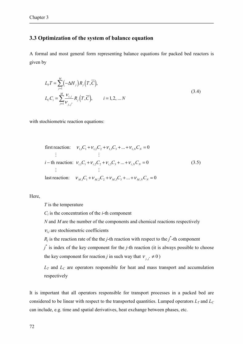
A formal and most general form representing balance equations for packed bed reactors is

given by

( ) ( )

( )*

1

,

1 ,

, ,

, , 1,2, ...

M

T j jj

Mi j

C i jj j j

L T H R T C

L C R T C i Nνν

=

=

= −∆

= =

∑

∑

(3.4)

with stochiometric reaction equations:

1,1 1 1,2 2 1,3 3 1,

,1 1 ,2 2 ,3 3 ,

,1 1 ,2 2 ,3 3 ,

first reaction: ... 0

th reaction: ... 0

last reaction: ... 0

N N

i i i i N N

M M M M N N

C C C C

i C C C C

C C C C

ν ν ν ν

ν ν ν ν

ν ν ν ν

+ + + + =

− + + + + =

+ + + + =

� �

� �

(3.5)

Here,

T is the temperature

Ci is the concentration of the i-th component

N and M are the number of the components and chemical reactions respectively

νi,j are stochiometric coefficients

Rj is the reaction rate of the the j-th reaction with respect to the j*-th component

j* is index of the key component for the j-th reaction (it is always possible to choose

the key component for reaction j in such way that *, 0j jν ≠ )

LT and LC are operators responsible for heat and mass transport and accumulation

respectively

It is important that all operators responsible for transport processes in a packed bed are

considered to be linear with respect to the transported quantities. Lumped operators LT and LC

can include, e.g. time and spatial derivatives, heat exchange between phases, etc.

Numerical methods

73

There are two ways to proceed with the numerical solution of system (3.4) and (3.5). The first

way is to solve the balance equations for each component Ci, i.e. to solve N + 1 equations.

Obviously, due to a possibly large number of components, and hence, equations, this is not a

very efficient way. The second way is to abstract from the linear algebraic system (3.5)

linearly independent components, to solve the balance equations only for these independent

components and then calculate the concentrations of the remaining components from the

stochiometric balance equations (3.5). However, even for a system with 15-20 components

finding a linearly independent subsystem of (3.5) is not an effortless task. Therefore, a simple

method has been developed to avoid extraction of a linearly independent subsystem.

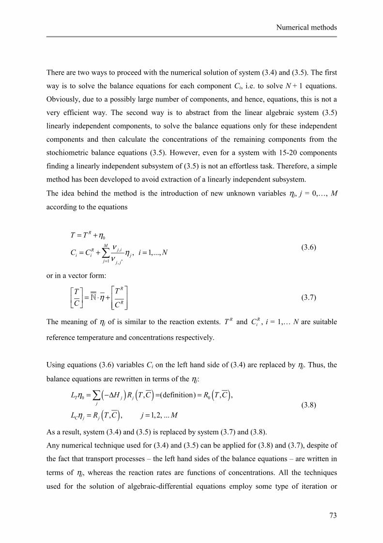
The idea behind the method is the introduction of new unknown variables ηj, j = 0,…, M

according to the equations

*

0

,

1 ,

, 1,...,

R

Mj iR

i i jj j j

T T

C C i N

ην

ην=

= +

= + =∑ (3.6)

or in a vector form: R

R

TTC C

η

= ⋅ +

� (3.7)

The meaning of ηj of is similar to the reaction extents. RT and RiC , i = 1,… N are suitable

reference temperature and concentrations respectively.

Using equations (3.6) variables Ci on the left hand side of (3.4) are replaced by ηj. Thus, the

balance equations are rewritten in terms of the ηj:

( ) ( ) ( )( )

0 0, (definition) , ,

, , 1,2, ...

T j jj

C j j

L H R T C R T C

L R T C j M

η

η

= −∆ = =

= =

∑ (3.8)

As a result, system (3.4) and (3.5) is replaced by system (3.7) and (3.8).

Any numerical technique used for (3.4) and (3.5) can be applied for (3.8) and (3.7), despite of

the fact that transport processes – the left hand sides of the balance equations – are written in

terms of ηj, whereas the reaction rates are functions of concentrations. All the techniques

used for the solution of algebraic-differential equations employ some type of iteration or

Chapter 3

74

marching, so that these methods can be easily adapted for the new system. Implicitness of the

methods can also be managed here for the new system of equations. The main distinction

from the implicit method employed for the original system (3.4) is in the calculation of the

Jacobi matrix. Schematically the Jacobian is calculated according to the following procedure.

Denote

,

ˆˆ ˆ,

ˆ

, , 0,...,

ˆ ˆ ˆ, 0,... , 0,...,

ii j

j

ii j

j

RJ i j M

RJ i M j N

C

η∂= =∂

∂= = =∂

then for i,j = 1,…, M

and

( )

( )

,0

0,0 ,01

0, ,1

, 1,...,ii

M

k kkM

j k k jk

RJ i MT

J H J

J H J

=

=

∂= =∂

= −∆

= −∆

∑

∑

Special care in the implementation of the new approach should be paid to the incorporation of

the boundary conditions. The boundary conditions might be given in terms of “external”

concentrations C-∞ and C∞, which have no relation to the stochiometric equations.

Rewriting the balance equations in form (3.8) and (3.7) has several advantages. First of all, as

a result of the transformation the least number of differential equations is solved. This

minimal number is equal to the number of reactions. The second merit of the proposed

approach is the automatic selection of the balance equations, i.e. there is no need to extract

linearly independent components from the system (3.5). This is of particular importance for

the “black-box” type packages. The user has only to supply stochiometric equations and the

Ji,j =

ˆ ˆ,ˆ

i jJ

�

*

Numerical methods

75

corresponding kinetics for the each reaction. Finally, the approach avoids the numerical

differentiation of sum ,

,

i jj

j jR

νν∑ present in the right hand side of the second equation of (3.4)

. This differentiation of the system might be inaccurate and might cause troubles because

each term in the sum has its own characteristic time scales. Of course, these troubles could be

also avoided by changing the order of the differentiation and the summation.

3.4 Coupling between solid and fluid phase equations

In this section a technique for efficient solution of the heterogeneous model equations is

presented. The goal is to incorporate the solid phase equations into the numerical algorithm

designed for the solution of corresponding homogeneous model equations. The technique will

be described for a most often used 2-D heterogeneous model, given by the balance equations

for:

the fluid phase:

( )

( )i

sers f p f v

si er is f v i

T Tu c r h a T Tz r r r

C D Cu r k a C Cz r r r

λρ ∂ ∂ ∂ − = − ∂ ∂ ∂

∂ ∂ ∂ − = − ∂ ∂ ∂

(3.9)

the solid phase:

( )( )

( , )

( , )i

s s sf v T

s s sf v i i

h a T T R C T

k a C C R C T

− =

− = − (3.10)

boundary conditions:

Chapter 3

76

( )

0 00 : ,

0 : 0, 0,

: , 0,t r w w

z T T C CT Crr r

T Cr R h T Tr r

λ

= = =∂ ∂= = =∂ ∂

∂ ∂= = − − =∂ ∂

(3.11)

Second order approximation of the spatial derivatives in the radial direction

1

1

2

1 121 1 1 1

2 2 2( ) ( )

j

j

j j

r r j j

j j jj j j j j j j jr r

u uur dr dr

u u u ur dr dr dr dr dr dr dr dr

+

= −

+ −− − − −=

−∂ =∂ +

∂ = − +∂ + +

(3.12)

yields a system of algebraic-differential equations of the following form:

( )

( )

sfy Dy k z yz

z y f z

∂ = + −∂− =

(3.13)

Here rj, j = 0…Nr, are the radial positions of the grid points and drj = rj+1 - rj.

( ) ( )0 1 0 1

1 1

, , ... , , , ...

( , , ..., ) , ( , , ..., )r r

T T

N N

T s s s Tj M j M

y y y y z z z z

y T C C z T C C

= =

= = (3.14)

D is a (M+1)(Nr+1) x (M+1)(Nr+1) tridiagonal matrix resulting from the discretization

(3.12) of the radial derivatives in (3.9).

M is the number of components in the system (in fact, in view of section 3.2, M is the number

of reactions), superscript T denotes transposition, k is a diagonal (M+1)(Nr+1) x

(M+1)(Nr+1) matrix determining solid-fluid heat and mass transfer, D is a tridiagonal matrix

resulting from the discretization of diffusion terms, and vector function f refers to the

reaction rates and the heat production rate.

Because of the reasons discussed in section 3.1 the derivatives in axial ditection appearing in

(3.14) are approximated by the implicit trapezoidal rule. As a result (3.14) is transformed to a

system of 2(M+1)(Nr+1) algebraic equations with the same number of unknown variables:

Numerical methods

77

( ) ( ) ( ) ( )( ) ( )

0 0 0 0 0 0

0 0

, , , 02

, , , 0

f sf sf

s

hF y z y z y y D y y k z y k z y

F y z y z y z f z

= − + + + − + − =

= − + = (3.15)

where h is the axial step size, 0 0,y z are known.

The powerful Newton-Kantorovich method is applied to solve this system of nonlinear

equations. The method applied to (3.15) is given by:

( )( )

0 0

0 0

1

1

, , ,/ // / , , ,

n nff f

n ns s sn

n n

n n

F y z y zyF y F zzF y F z F y z y z

y y yz z z

δδ

δδ

+

+

∂ ∂ ∂ ∂ = − ∂ ∂ ∂ ∂

= +

= +

(3.16)

with known ,n ny z .

The specific properties of system (3.16) are utilized to efficiently solve the equations. Note

that

,

2 2

,

f fsf sf

s s

F Fh hI D k ky z

F FI I Jy z

∂ ∂ = − + − = ⋅ ∂ ∂

∂ ∂= = − +∂ ∂

(3.17)

with I as the unity (M+1)x(M+1) matrix and /J f z= ∂ ∂ .

Using (3.17) system (3.16) is splitted into two systems, which are solved consecutively.

Firstly the fluid phase equations are solved from

( )

( ) ( ) ( )

1

10 0 0 0

2 2 2

, , , , , ,2

sf sf

n

n n n nf ssf

h h hI D k k I J y

hF y z y z k I J F y z y z

δ−

−

− + − − =

= + −

(3.18)

and subsequently the equations for the solid phase given below are solved

( ) ( )1 0 0, , ,n nsn

z I J y F y z y zδ δ− = − + (3.19)

Chapter 3

78

System (3.18) has the same structure as that obtained from the corresponding homogeneous

model; namely, a block tridiagonal matrix with diagonal sub and upper diagonal blocks. It is

a sparse system of linear equations that can be efficiently solved with the number of

operations proportional to M3Nr. The procedure for solving such types of linear algebraic

systems is described in the next section. Arrangement of the state variables in the order given

by (3.14) and splitting of the system into two subsystems (3.18) and (3.19) (to be solved

consecutively) allows the application of all numerical techniques developed for homogeneous

systems also to heterogeneous systems.

3.5 Solution of systems with diffusion terms

The presence of diffusive terms in the system of model equations has a two-fold effect on

their numerical treatment. On one side, the diffusion smoothens the solution and reduces

difficulties associated with the approximation of the convection terms. On the other hand, the

diffusive terms demand implicit approximation schemes to avoid too small time steps, which

ultimately lead to large systems of algebraic equations. A numerical technique for the

solution of algebraic equations resulting from the discretization of diffusive terms is

described in this section. The technique is described on the basis of a 1-D non-steady state

homogeneous model

( )2

12

DU U U R Ut z z

∂ ∂ ∂+ − =∂ ∂ ∂zΛ D (3.20)

This section focuses on the effect of diffusion terms, although usually in packed bed reactors

convection is the dominant transport mechanism. Discretization of convection terms requires

special techniques that will be considered in Chapter 4. Here, it is simply assumed that the

approximation

( ) ( )1/ 2 1/ 2

n n

i i

i

U UUz z

+ −−∂ ≈

∂ ∆Λ Λ

Numerical methods

79

is sufficiently accurate and no further details of it are considered. Also note that the presented

algorithm is also valid for the solution of 2-D steady state model equations. In addition,

following the discussion in previous section, the method can be easily extended to the

heterogeneous models.

In the following, system (3.20) will be solved subject to the following general boundary

conditions:

0 :

1:

L L

R R

yz A y Bzyz A y Bz

∂= = +∂∂= = +∂

(3.21)

Discretization of the system is done by explicit (at time tn) approximation of the convection

term, implicit (at time tn + ∆t) approximation of the diffusive term and Heun’s type of time

stepping, i.e.

( ) ( ) ( )1

1 1 11/ 2 1/ 2

n nni Di i i i

ii

U UU U U R Ut z

+ −−− + − =

∆ ∆ z

Λ ΛD (3.22)

( ) ( ) ( ) ( )1 11 1

1 1 11/ 2 1/ 20.5

, 1, , 1/ 2

n ni i i i Di i

ii

U U U U UU R U i N

t z

++ −

− + −+ − = = −

∆ ∆ z

Λ ΛD … (3.23)

Here izD is the discrete operator approximating the diffusive term. The computational grid is

defined in such a way that the boundaries coincide with the cell center of the first and the last

cells, i.e. a mesh of type II is used (see section 4.3.5).

Due to the strong non-linearity of the reaction rates, the right hand side of (3.22) is linearized

and the system is solved by Newton iterations. The solution of (3.22) –which is in fact the

first order Euler approximation of (3.20)- is upgraded to second order using relation (3.23).

The correction is “computationally cheap” because no iterations are needed and no linear

algebraic system needs to be solved. On the contrary, (3.22) is a system of (Nz+1).(M+1) x

(Nz+1).(M+1) nonlinear algebraic equations, the solution of which involves both iterations

and large matrix inversions. Nz is the number of cells in the computational domain; M is the

number of reactions. Discrete operator izD determines the structure of the system. The

diffusive terms are discretized according to

Chapter 3

80

2

1 121 1 1 1

2 2 2( ) ( )

i

j j ji i i i i i i iz z

u u u uz z z z z z z z z+ −

− − − −=

∂ ≈ − +∂ ∆ ∆ + ∆ ∆ ∆ ∆ ∆ + ∆

(3.24)

The derivatives at the boundaries (i = 0 and i = Nz) are discretized using second order

approximations

0 1 20 0 0 1 0 0 1

1 21 1 2 1 1 2

2 1 2 1

2 1 2 1z z z

z z z z z z z

z

N N Nz N N N N N N N

u u u uz z z z z z z

u u u uz z z z z z z

=

− −= − − − − − −

∂ ≈ − + + − ∂ ∆ ∆ + ∆ ∆ ∆ + ∆

∂ ≈ − − + ∂ ∆ ∆ + ∆ ∆ ∆ + ∆

(3.25)

System (3.22) and boundary conditions (3.21) make up a system of nonlinear equations

( )0 0 0 0 1 0 2 0, 0nF y y C y B y A y E= + + + =

( ) ( ) ( )1, 0, 1, , 1n n n Dii i i i i zF y y y y t Conv y tD y tR y i N= − + ∆ − ∆ − ∆ = = −… (3.26)

( ) 1 2, 0z z z z z z z z

nN N N N N N N NF y y C y B y A y E− −= + + + =

Constant (M+1) x (M+1) matrices A0,Nz, B0,Nz, C0,Nz and E0,Nz are determined by boundary

conditions (3.21) and approximations (3.25).

Here

( ) ( )1 1 1 1 10 1, , , , , , ,

z

T TMN i i i iy U U U U T C C= =… …

Conv (yn) is the numerical operator representing the approximation of the flux derivatives. D

is a tridiagonal (Nz+1).(M+1) x (Nz-1).(M+1) matrix determined by discretization (3.25).

Newton’s method applied to (3.26) reads

( ) ( ),,

k nk k k n

k

F y yy y F y y

yδ δ

∂≡ = −

∂A (3.27)

1k k ky y yδ+ = +

Numerical methods

81

where the starting values of y are taken from the n-th time level, i.e. y0 = yn and the

converged yk determines the solution y1. Matrix A is “almost” block-tridiagonal. Only the

first and the last (M+1) rows break up this structure.

0 0 0

1 1 1

2 2 2

2 2 2

1 1 1

z z z

z z z

z z z

N N N

N N N

N N N

C B AC B A

C B A

C B AC B AC B A

− − −

− − −

=

A � � �

Moreover, matrices Ai, Ci, , i = 0…Nr, B0, BNr are diagonal.

“Almost” block-tridiagonal system (3.27) is solved by a method, which can be considered as

a modification of the Thomas’ algorithm for tridiagonal systems. Each scalar ai, bi, and ci, in

the Thomas’ algorithm is replaced by matrices Ai, Bi, and Ci, and care is taken for the first

and the last (M +1) rows of matrix A .

Provided that all matrices involved are invertible – as always for the packed bed reaction

problems – system (3.27) is equivalent to the following system of equations:

[ ][ ] [ ]

0 0 0 1 0 2

1 11

1

11 1

1 2

0

, 1

0z z z z z z

i i i i z

i i i i i

i i i i i i i

N N N N N N

C y B y A y

y L y K i N

L C L B A

K C L B F C K

C y B y A y

δ δ δ

δ δ

δ δ δ

− −−

−

−− −

− −

+ + =

= + = = − +

= + −

+ + =

…

(3.28)

To permit the use of the “sweeping” technique to solve (3.28), i.e. to calculate Li and Ki from

left to right and then calculate δyi from right to left, values of L0, K0 and Nzyδ are required.

L0, K0 can be calculated using the first 2(M+1) equations of (3.27) and Nzyδ is calculated

using the last 2(M+1) equations of (3.27). As a result the relations

Chapter 3

82

1 11 1 1 10 1 1 0 0 1 1 0 0 1 1 1 0 0 1 1 0 0y C A A C B A A B y C A A C F A A Fδ δ

− −− − − − = − − − + − −

( )( )

1 11 1 1 1 1

1 11 1 1 1 1

z z z z z z z z z z

z z z z z z z z z

N N N N N N N N N N

N N N N N N N N N

A C C A B C C B L y

F C C F B C C B K

δ− −− − − − −

− −− − − − −

− + − =

− − −

are obtained. The first set of equations yields

11 1

0 1 1 0 0 1 1 0 0

11 10 1 1 0 0 1 1 0 0

L C A A C B A A B

K C A A C F A A F

−− −

−− −

= − − −

= − −

(3.29)

The second set of equations determines Nzyδ as

( )( )

11 11 1 1 1 1

1 11 1 1 1 1

z z z z z z z z z z

z z z z z z z z z

N N N N N N N N N N

N N N N N N N N N

y A C C A B C C B L

F C C F B C C B K

δ−− −

− − − − −

− −− − − − −

= − + − ×

× − − −

(3.30)

Having L0 and K0 calculated by (3.29) Li and Ki are calculated for all i = 1… Nz according to

the third and the fourth equations of (3.28). Then, having Nzyδ calculated by (3.30) and

knowning Li, Ki, the second equation of (3.28) is used to calculate δyi for i = 0…Nz – 1.

It should be noted that most of the matrices involved in this algorithm are diagonal, and

therefore, many matrix multiplications and inversions involve in fact only few operations.

3.6. Summary and Conclusions

In this chapter numerical techniques dealing with the most salient numerical problems

specific to packed bed reactor model equations have been considered. All the techniques have

rigorous mathematical justification and have been implemented in “PackSim”, a software

package specially developed for packed bed reactor modeling.

The first numerical problem considered in this chapter is the problem of large differences in

characteristic time scales for different reactions (stiffness), which is a serious problem in

many physical-chemical systems. In this work a stiff nonlinear equations solver is combined

with a simple and efficient automatic time step size control algorithm. The proposed method

was developed for the solution of ODEs resulting from the spatial discretization of partial

differential equations. It is very common that the spatial discretization of PDEs involves

Numerical methods

83

sophisticated techniques and requires significant computer resources and computational time.

Therefore, the presented ODE solver is developed in such a way that it is simple enough to be

incorporated in PDE solvers and robust enough to efficiently solve ODEs. The capabilities of

the method have been demonstrated solving an extremely stiff ODE system.

The second problem specific to the packed bed reactor model equations and considered here

is related to the large number of equations to be solved. A technique is proposed to optimize

the number of governing partial differential equations before solving them numerically. The

algorithm introduces new dependent variables (instead of unknown concentrations), which

are “independently” transported and accumulated. The concentrations of all the components

are calculated from these new variables, which is used in the evaluation reaction rate

expressions. It has been shown that the technique assures the solution of the minimum

possible number of equations. This is especially useful in case of a large number of

components and reactions in order to minimize the usage of computer resources and

computational time. Furthermore, the technique also allows automatic selection of the

differential equations to be solved, whereas the concentrations of the remaining components

are calculated using stochiometric equations.

Another technique has been proposed to incorporate solid phase balance equations into the

solution procedure designed to solve pseudo-homogeneous model equations The method

allows decoupling of fluid and solid phase equations in such a way that the large system of

finite-difference equations is solved in two consecutive steps. In each step a much smaller

system is solved. The method is especially efficient if the discretization results in structured

sparse matrices. In addition, it allows a straightforward extension of the numerical programs

developed for the solution of homogeneous systems to algorithms for heterogeneous systems.

Finally, an efficient solver for sparse linear algebraic equation systems resulting from the

discretization of diffusion-type equations is developed. The method effectively incorporates

the boundary conditions typical for these types of equations. The technique is especially

beneficial, if the number of the reactions is much less than the number of nodes in the

computational grid.

In the next chapter the remaining numerical problems listed in the introduction to this chapter

will be addressed.

Chapter 3

84

CHAPTER 4

Numerical methods for the solution of the wave and convection dominated diffusion type models

Chapter 4

86

Abstract Equation Section 4An ENO based numerical method for the solution of the non-steady state

wave and the convection dominated diffusion type models has been developed. Special

attention is paid to the discretization of the convection terms. The proposed method

extensively takes into account physical and mathematical features of the models and

produces accurate and stable results. An algorithm for the approximation of one-dimensional

scalar nonlinear equation is first described. The algorithm is then extended to two-

dimensional systems of equations. The method allows efficient integration of the convective

term in combination with the diffusion and source terms.

An efficient mesh adaptation technique has been developed to further enhance the

capabilities of the method. The method satisfies a list of criteria for mesh adaptation

techniques. The method extensively uses data already computed for the ENO discretization

and conserves all the beneficial properties of the ENO scheme. The technique is developed

and described for one- and two-dimensional problems and can be extended to 3-D problems.

The advantages of the numerical method are demonstrated using several test cases.

Convection terms

87

4.1 Introduction

Continuum models describing transport phenomena in packed bed reactors have been

considered in chapter 2. Generally, the models are presented in the form of a set of Partial

Differential Equations (PDE) containing time and space derivatives. The models incorporate

a variety of interconnected chemical and physical processes. The complexity of the real

processes taking place in the reactor not only leads to uncertainties and difficulties with their

mathematical description, but also to considerable problems in the numerical treatment of the

resulting equations. The numerical difficulties specific for this type of PDE’s are:

8. Large differences in characteristic times for different reactions (reaction

stiffness) and physical processes

9. Large number of equations

10. Strong sparsity of matrices involved

11. Numerical diffusion introduced by convection approximations

12. Non-physical oscillations near steep gradients and discontinuities

13. Reasonably looking but fake solutions

14. Strongly coupled equations resulting from coupling between physical and

chemical processes

The first three of the aforementioned numerical problems have already been addressed in

Chapter 3. This chapter will focus on the last four of the listed difficulties. These problems

require specific attention especially when solving the wave model equations, which will be

considered in the next chapter, since they constitute a hyperbolic PDE system. Hyperbolic

equations do not smoothen steep gradients and discontinuities and, moreover, smooth initial

data can evolve into shock waves, thus requiring special numerical solution techniques. Also

the solutions of convection-dominated standard dispersion models (SDM) require special

methods to handle very steep gradients and discontinuities. Problems associated with the

numerical treatment of such models are in the focus of this chapter.

Chapter 4

88

The application of the numerical method developed in this chapter is not restricted to packed

bed model equations only. The technique can also be applied to a variety of fluid dynamics

problems, where the vector of unknowns U is given in the following general form:

( ) ( ) ( , ) ( , ) ( )d dU F U G U F U U G U U R Ut x y x y

∂ ∂ ∂ ∂ ∇ ∂ ∇+ + = + +∂ ∂ ∂ ∂ ∂

(4.1)

Here the vector-functions F(U) and G(U) represent convective fluxes, the vector-functions

Fd(U,∇U) and Gd(U,∇U) account for diffusion effects and R(U) represents the vector of

source terms.

Both the wave and the standard dispersion model can be presented in this general form, see

Table 4.1.

Even though the convection fluxes F(U) and G(U) in the SDM and the wave model are linear

with respect to the state variables, the method designed in this chapter is also capable of

solving systems with general non-linear fluxes. Actually, the code was tested for Euler

equations of fluid dynamics and a few other fluid dynamics problems, where the convection

fluxes are non-linear. The only fundamental restriction imposed on system (4.1) is the

requirement of diagonalizability of the matrices ( )F UU

∂∂

and ( )G UU

∂∂

for any U in the domain

of interest. In other words, it is required that for every U there must exist matrices �, ,Z Z

Y and �Y such that � FU∂∂

Z Z and � GU∂∂

Y Y are diagonal. In physical terms this requirement

means that transported quantities can be regrouped in such a way that each combination is

independently convected in a certain characteristic direction with a certain characteristic

speed. The speed of propagation is determined by the diagonal elements (eigenvalues) of

matrices ( )F UU

∂∂

and ( )G UU

∂∂

.

If all their eigenvalues are real and different, then, it is guaranteed that the matrices are

diagonalizable, however, this is not a necessary condition. For example, packed bed reactor

models involving multi-component fluids consist of equations where the matrices have

multiple equal eigenvalues. Nevertheless, it is possible to diagonalize this system, since the

balance equations are coupled via the reaction rate terms and the “components” are convected

“independently”.

Convection terms

89

Table 4.3. Representation of the standard dispersion and the wave models in the form of general system (4.1).

Standard dispersion model Wave model

Vector of

unknowns U = (T, C)T U = (T, C, jmr, jmr, jmr, jmr)T

Equations 2

2

1( )z r

U U U Ur R U

t z z r r r∂ ∂ ∂ ∂ ∂

+ = + +∂ ∂ ∂ ∂ ∂

Λ D D ( )U U U

R Ut z r

∂ ∂ ∂+ + =

∂ ∂ ∂A B

Matrices

Λ, Dz, Dr are diagonal matrices

11 12

21 22

33

=

A A 0A A A 0

0 0 A

13

31

=

0 0 BB 0 0 0

B 0 0

R(U) ( , )

( )( , )

T

C

f C TR U

f C T

=

( , )( , )

( )

T

C

hz

mz

hr

mr

f C Tf C T

fR U

fff

=

Λ, Dz, Dr, Aij are (M+1) x (M+1) matrices defined in Appendix 4.A

M is the number of reactions. Superscript T denotes the transposition operation. Other

information about the two systems is given in Appendix 4.A

In chapter 3 some salient problems specific for convection-diffusion-reaction systems have

been considered. A technique for the automatic selection of the optimal number of

independent balance equations has been proposed. In addition, an efficient and easy to

implement method of coupling of the fluid and solid phase balance equations has been

developed. This chapter focuses on the construction of an effective and trustworthy method

for the approximation of the convection terms and their coupling with the diffusion and

source terms and the boundary conditions In Section 4.2 the main difficulties encountered in

the numerical treatment of several system of type (4.1) are systematically discussed. This

Chapter 4

90

section is concluded with a list of criteria that should be satisfied in order to construct a

reliable and efficient numerical solver. An Essentially Non-Oscillatory (ENO) scheme for the

solution of hyperbolic (wave) and convection dominated parabolic (diffusion-type) equations

is constructed in Section 4.3. In this section firstly a 1-D linear scalar equation is considered,

which is consequently extended to 2-D systems of non-linear equations. The section is

completed by the description of the numerical treatment of the boundary conditions and the

diffusion and source terms. An efficient 1-D and 2-D mesh adaptation technique has been

developed reckoning the specific properties of the ENO scheme. The technique automatically

adjusts the computational grid to the solution being calculated and by that optimizes the

calculations. The mesh adaptation technique is described in Section 4.4 for 1-D and 2-D

systems. The technique can easily be extended to 3-D systems.

4.2 Approximation of the convection terms

Calculation of the convection of some physical quantity from one location to another may

demands more of the numerical technique than the simulation of other effects, such as

diffusion or reaction. One of the reasons is the absence of natural smoothing of profiles in the

calculations of the convection terms. In fact an opposite effect might occur: discontinuous

(weak) solutions may emerge from initially smooth data. From physical considerations,

convection is subjected to constraints of positivity, conservation and time reversibility.

Therefore, preferably these constraints should be inherently incorporated into the numerical

algorithm to calculate the convection terms. Problems encountered in the numerical treatment

of the convection terms are described in the following subsections, from which requirements

on the numerical methods are deduced to overcome the problem in the approximation of

convection terms.

4.2.1 Finite propagation speed and the CFL condition

Consider a hyperbolic system of two linear equations

0

0

u at x

uat x

ν

ν

∂ ∂+ =∂ ∂∂ ∂+ =∂ ∂

(4.2)

with initial data u(0,x) = u0(x) and v(0,x) = v0(x) to illustrate the idea of a finite signal

propagation speed and its effect on the numerical approximation.

Convection terms

91

The exact solution of the system is given by:

( ) ( ) ( ) ( )

( ) ( ) ( ) ( )

0 0 0 0

0 0 0 0

( , )2 2

( , )2 2

u x at v x at u x at v x atu t x

u x at v x at u x at v x atv t x

− + − + − += +

− + − + − += −

(4.3)

Solution (4.3) shows that the initial information about functions u and v (u0 and v0)

propagates along the characteristic lines of the system (4.2), given by x ± at = const with a

finite speed a. Thus, the solution at point (t, x) is uniquely determined if the initial data at x0

= x – at and x1 = x + at are known, and vice versa, the initial data at point x0 influence the

solution only along two characteristic lines: x – at = x0 and x + at = x0. Qualitatively these

properties are valid for the general hyperbolic system given below.

0U Ut x

∂ ∂+ =∂ ∂

A (4.4)

Figure 27. Schematic representation of the domain of dependence and the range of influence for hyperbolic systems.

The speed and the direction of signal propagation are determined by the eigenvalues of

matrix A. The solution of the system at point A(t, x) is completely determined by the initial

data in the interval [B, C], as indicated in Figure 27. Here amin and amax denote the minimal

and the maximal eigenvalues of matrix A, respectively. Characteristic lines x - amin t = const

and x - amax t = const bound the domain of dependence of point A. In other words, the

solution of the general hyperbolic system (4.4) at point A depends only on the solution in the

(t, x)

x a max t = const x amin t =const

(t0 0)B P Q C

A

x amin t =const x max t =const

x

t

Domain of epende nceof point ( )

Range influen of point ( 0 0

- -

,x

- - a

d t,x

of ce t ,x )

Chapter 4

92

interior of the triangle ABC, and points outside ABC do not effect the solution at this point.

Inversely, the influence of the initial data at point (t0, x0) can not spread beyond the region

bounded by the characteristic lines originating from (t0, x0), i.e. the range of influence of

point (t0, x0) is bounded by the two characteristic lines lying furthest apart, see Figure 27.

These fundamental properties of hyperbolic systems must be taken into account in the

construction of a numerical approximation of the equations. The criterion linking the above

considered mathematical properties of the system to the properties of its finite-difference

approximation is called the Courant-Friedrichs-Lewy (CFL) condition. The CFL sets a

restriction on the ratio of temporal and spatial discretization steps

( )min maxt max | |, | |CFL 1

xa a∆

= <∆

(4.5)

The CFL criterion states that the numerical scheme will not converge, if the domain of

dependency of the system is larger than the domain of dependency of its numerical

approximation. Indeed, if triangle ABC in Figure 27 is the domain of dependence of exact

solution U(t,x), APQ is the domain of dependence of its numerical approximation Uh(t,x),

then changing initial data in the intervals BP and QC can influence U at (t, x), but the

numerical solution at (t,x) will not be effected. This means that Uh(t, x) cannot converge to

the exact solution U(t, x). In fact, Courant, Friedrichs and Lewy (1928, 1967) derived the

condition in the course of proving the existence of the exact solutions of certain PDE’s using

their finite-difference analogs. It is important to realize that the CFL condition is only a

necessary, but not sufficient condition for numerical stability. Although CFL = 1 may suffice

in some cases, generally a more strict condition (CFL ≈ 0.4-0.8) is applied in practice.

4.2.2 Upwind differencing If a piece-wise constant profile (e.g. a concentration or temperature profile), depicted in

Figure 28, is moving according to the advection equation

0 with 0u ua at x

∂ ∂+ = >∂ ∂

(4.6)

Convection terms

93

the front moves either in the positive or the negative x-direction without any change of front

shape. The direction is determined by the sign of a; a positive value of a corresponds the

movement of the front in the positive direction. The direction of signal propagation should be

taken into account when constructing the computational stencil.

Figure 28. Concentration front moving according to the advection equation.

For example, when using centered differencing (stencil shown in Figure 29a), the numerical

solution at (n+1, j) is strongly influenced by the value at (n, j+1). This is, however,

physically unsound and leads to instabilities in the calculations. In contrast, the “upwind”

discretization scheme (stencil depicted in Figure 29b), does not use the value at (n, j+1) and

tracks the initial data in the physically correct direction and is stable, provided that the CFL

condition has been satisfied.

Figure 29. Stencils for numerical discretization of the advection equation: a) centered differencing, b) upwind differencing.

u

x

1

0 t = t1 -dt t = t1 t = t1 +dt

j-1

t n+1

j j +1

n

a)

x

n+1

j-1 j

n

b)

t

x

Chapter 4

94

Similar considerations hold for any hyperbolic system of equations. Proper rearrangement of

unknown vector-functions results in a set of new (characteristic) variables that propagate

along their characteristic lines. Each characteristic variable propagates in its own direction

and should be approximated in upwind fashion (in their characteristic direction). However, in

practice the requirement of strict upwinding is too restrictive from the point of view of

approximation accuracy. Usually small “smart” downwind influence can be tolerated.

4.2.3 Discontinuous solutions and monotone schemes

One of the features of the hyperbolic equations that greatly complicates their numerical

treatment is that discontinuities or very steep gradients do not diffuse and smoothen in time.

Moreover, even smooth initial data can evolve into discontinuous solutions. Difficulties with

handling of discontinuities can be encountered even for the simplest advection equation (4.6)

as considered in the previous subsection. This equation accompanied with the initial data

given by

1 0

(0, )0 0

xu x

x<

= >

can be solved using a first order accurate upwind scheme with stencil depicted in Figure 29b:

( )11

n n n nj j j j

tu u a u ux

+−

∆= − −∆

(4.7)

In Figure 30 the numerical solution calculated with CFL = 0.5 is compared with the analytical

solution.

Figure 30. Comparison of the exact and a first order numerical approximation of the advection equation at t = 0.5 (a = 1, ∆t = 0.01, ∆x = 0.02, CFL = 0.5).

0 0.2 0.4 0.6 0.8 1x

u

0

0.2

0.4

0.6

0.8

1Exact solution

First order upwind scheme

Convection terms

95

-0.2

0

0.2

0.4

0.6

0.8

1

1.2

0 0.2 0.4 0.6 0.8 1x

uBeam-Warming

Exact solution

-0.2

0

0.2

0.4

0.6

0.8

1

1.2

0 0.2 0.4 0.6 0.8 1x

u

Exact solution

Lax-Wendroff

The figure clearly demonstrates a significant approximation error introduced by this scheme.

The discontinuity is smeared and ultimately the numerical solution may become irrelevant to

the exact solution.

The reason for this departure is the artificial diffusion introduced by the numerical

approximation. Indeed, the Taylor series of the solution of (4.6) is

( ) ( ) ( ) ( ) ( ) ( )2 2 2

32

, ,, ,

2u x t t a u x t

u x t t u x t ta O tx x

∂ ∆ ∂+ ∆ = −∆ + + ∆

∂ ∂ (4.8)

The first order upwind difference scheme (4.7) does not approximate the second derivatives

present in the expansion, therefore, the truncation error of the scheme has diffusion type form

( )2

22

uO xx∂∆∂

which smoothens the discontinuity in the profile. Many widely used second

order schemes solve the problem of numerical diffusion by adding terms approximating the

diffusional term in the Taylor expansion (4.8). Two popular representatives of such schemes

are:

the Lax-Wendroff (1964) scheme

( ) ( )2

11 1 1 1

1 22

n n n n n n nj j j j j j j

ta tu u u u a u u ux x

++ − + −

∆ ∆ = − − + − + ∆ ∆

and the Beam-Warming (1978) scheme

( ) ( )2

11 2 1 2

13 4 22 2

n n n n n n n nj j j j j j j j

ta a tu u u u u u u ux x

+− − − −

∆ ∆ = − − + + − + ∆ ∆

Figure 31 shows the approximation to the advection equation using these second order

schemes.

Figure 31. Comparison of the exact and second order numerical approximations of the advection equation at t = 0.5 (a = 1, ∆t = 0.01, ∆x = 0.02, CFL = 0.5).

Chapter 4

96

The fundamental problem arising with the application of higher order difference schemes is

the appearance of non-physical oscillations deteriorating the solution (referred as the Gibbs

phenomenon). The oscillations are caused by the so-called numerical dispersion, which can

explained mathematically using the von Neumann analysis. Briefly, the analysis is based on a

Fourier series of the solution at time level n, which is evolved to level n + 1 according to one

of the abovementioned schemes. Ideally, all the terms in the Fourier series would propagate

with the same speed a. However, with the mentioned second order schemes some terms lag

and some terms lead, which results in oscillations in the numerical solution. The oscillations

cannot be eliminated by refining the computational grid.

The problem of numerical dispersion does not appear if the scheme is monotone, i.e. if n nj jv u≥ for all j then 1 1n n

j jv u+ +≥ for all j. The first order upwind scheme is a monotone

scheme and, therefore, does not produce numerical oscillations. The Lax-Wendroff and

Beam-Warming schemes are not monotone and do give oscillating solutions. Moreover,

generally, no scheme of order higher than one can be monotone. Although monotonicity

guaranties non-oscillatory behavior of a scheme, it is too restrictive to be always enforced.

Therefore, other (less restrictive) schemes with higher order accuracy, still guaranteeing non-

oscillatory behavior of the approximation, are very often used in practice:

• monotonicity preserving: schemes transforming a monotonic function un into a

monotonic function un+1 .

• L1 – contracting: time marching is done by an operator contracting in the discrete L1

space, |1 1

1 , 1n nL L

u uα α+ ≤ <

• Total Variation Diminishing (TVD): TV(un+1) ≤ TV(un). The numerical total variation

is defined as ( ) 1n n n

j jj

TV u u u∞

+=−∞

= −∑

• Essentially Non-Oscillating (ENO): TV(un+1) ≤ TV(un) +O(∆xr), where r indicates the

formal order of accuracy of the scheme.

• Total Variation Bounded (TVB): TV(un) ≤ M≤ 0 for all n.

Convection terms

97

4.2.4 Spurious solutions and conservative and consistent numerical schemes Even if all the above-described conditions are satisfied, the numerical approximation does not

guarantee the convergence of the numerical solution to the exact solution. The numerical

solutions of hyperbolic equations may even converge to a fake but seemingly realistic

solution. The missing link in the list of conditions to be satisfied, in order to construct a

reliable numerical method, regards conservativeness and consistency of the method.

A finite-difference method is called conservative, if the flux derivative approximation can be

presented as

( ) ( ) ( )1 1 1, , ..., , , ...,n n n n n nj p j p j q j p j p j qF U U U F U U Uf U

x h− − + − − − − − −−∂

≈∂

(4.9)

for some numerical flux function F of p+q+1 arguments. p and q determine the number of

nodes in the corresponding computational stencil. For example, if p = q = 0 then only two

nodes are used in the approximation. If in addition F(U) = aU and a > 0, then (4.9) is the first

order upwind approximation (4.7) of the advection equation. The numerical conservativeness

means that like the differential equations, also the difference equations conserve quantities in

each numerical cell.

A finite-difference method is called consistent, if the numerical flux is equal to the exact flux

for a constant function ( , )U t x U≡ :

( ) ( ), ,...,F U U U f U= (4.10)

The importance of the conservativeness can be illustrated based on the solution of Burger’s

equation

21 02

u ut x

∂ ∂ + = ∂ ∂ (4.11)

with the following boundary conditions

( ) 1.2 00,

0.4 0x

u xx<

= ≥

Numerical approximation is carried out with the following first order finite-difference

scheme

Chapter 4

98

1

1 0n n n nj j j jn

j

u u u uu

t x

+−− −

− =∆ ∆

(4.12)

Although the numerical solution correctly describes that the initial profile should travel to the

right, it fails to predict the correct speed with which the discontinuity should move, Figure

32. According to the Rankine-Hugoniot jump condition the speed of the moving discontinuity

should be

2 2 2 21 1 1 11.2 0.4

2 2 2 2 0.81.2 0.4

right left

right leftt

u us

u u

− ⋅ − ⋅= = =

− −

and the discontinuity should be located at x = 0.8 at t = 1.

Figure 32. Comparison of the exact and the numerical solution, calculated using a non-conservative method, to Burger’s equation at t =1 (∆t = 0.01, ∆x = 0.02, CFL = 0.5).

The failure of (4.12) to predict the correct propagation speed is due to its non-

conservativeness. Non-symmetry with respect to the left and right walls of the computational

cell in the approximation (4.12) induces a lower speed of the moving discontinuity in the

numerical solution.

The set of conditions listed above gives a guideline for a correct approximation of systems of

hyperbolic equations. Lax and Wendroff (1960) proved that if the numerical solution is

calculated by a conservative and consistent method, it will indeed approximate the exact

solution. The theorem, however, does not guarantee the convergence of the method.

In case of more complex systems including diffusion and reaction terms the behavior is more

complex. Therefore, a detailed investigation of the developed method for the solution of the

0 0.2 0.4 0.6 0.8 1x

u

Numerical solution

Exact solution

0

0.2

0.4

0.6

0.8

1

Convection terms

99

wave model equations is required and the numerical solution should be carefully tested to

ensure success of the method.

4.3 The numerical method In the following a comprehensive method for the solution of the general system of equations

(4.1) is developed and described. The method is based on the ENO scheme proposed by Shu

and Osher (1988, 1989). The scheme is adapted for the problems considered in this thesis by

incorporation of techniques for the treatment of the diffusive and source terms. The method

satisfies the criteria enumerated in the previous sections. It is relatively easy to extend the

scheme to multi-dimensions and to apply it on non-uniform computational meshes. The

superiority of the method over other widely used finite-difference schemes will be shown in

the derivation of the method and will be demonstrated for several test examples.

4.3.1 ENO scheme for a 1-D scalar equation

The ideas behind the Essentially Non-Oscillating (ENO) schemes are firstly described and

illustrated for a 1-D non-linear scalar equation

( ) 0f uu

t x∂∂ + =

∂ ∂ (4.13)

The scheme will be extended to multidimensional systems in the following sections.

A one-dimensional computational cell is depicted in Figure 33 to demonstrate the adopted

definitions.

Chapter 4

100

Figure 33. Schematic description of an one-dimensional computational cell.

In Figure 33 xi-1/2, xi+1/2 are the cell walls of the i-th cell and xi is the cell center of cell “i”. By

definition 1/ 2 1/ 2

2i i

ix xx + −+= and 1/ 2 1/ 2i i ix x x+ −∆ = − .

In 1959, Godunov proposed a method to make use of the characteristic information enclosed

in the equation in the framework of conservative methods. According to his approach the

numerical solution un is used to define a piecewise constant function ( ),n nu x t� with the value

niu on the i-th grid cell. Function ( ),n nu x t� is used as an initial value for the conservation

equation, which can be solved exactly (as the Riemann problem) over a small interval (tn,

tn+1). The exact solution over the entire interval is constructed by piecing together these

Riemann solutions. After obtaining ( )1,n nu x t +� , 1n

iu + is approximated by averaging this exact

solution at time tn+1

( )1/ 2

1/ 2

1 11 ,i

i

xn n ni x

i

u u x t dxx

+

−

+ +=∆ ∫ � (4.14)

These values are used to define a new piecewise constant function ( )1 1,n nu x t+ +� and the

process is repeated again to march in time.

In practice this algorithm can be considerably simplified by observing that the cell average

(4.14) can be easily computed using the integral form of (4.13). Since un is assumed to be

exact solution and ( ),n n niu x t u=� over the interval (xi-1/2, xi+1/2), integration of equation (4.13)

over a computational cell (xi-1/2, xi+1/2) x (tn, tn+1) gives

( ) ( )11/ 2 1/ 2

n n n ni i i i

i

tu u F u F ux

++ −

∆ = − − ∆ (4.15)

xi - 1/2 xi + 1/2

xi xi + 1 xi - 1

xi + 3/2

∆xi

cell walls cell center

∆xi + 1

Convection terms

101

where

( )( )1

1/ 2 1/ 21( ) ,n

n

tn ni it

F u f u x t dtt

+

+ +=∆ ∫ �

The resulting scheme is first order accurate. Higher order methods based on the Godunov

approach were developed by van Leer (1973, 1979). In the van Leer’s approach ( ),n nu x t� is

constructed as a linear function of x and gives a second order accurate approximation. Third

order accurate approximations are achieved by using the Piecewise-Parabolic Method (PPM)

of Woodward and Colella (1981,1985) and the second order with Uniformly Non-Oscillatory

(UNO) method of Harten et al. (1986) and Harten and Osher (1987). The latter schemes

served as the basis for the development of ENO schemes.

UNO schemes can also be presented in form (4.15). Although (4.15) gives the relation

between the cell-averages 1niu + and n

iu , the evaluation of the fluxes 1/ 2 ( )iF u+ requires

knowledge of the solution itself. Hence, a reconstruction procedure is needed to recover point

values from cell averages to the required order of accuracy, which can be rather complicated,

especially in multi-dimensional problems. A proper reconstruction of function u or flux F(u)

at the cell faces from the cell averaged (or cell centered) value of u is the crucial step in the

construction of conservative difference schemes.

Significant improvements of the uniformly high-order accurate non-oscillatory technique

were achieved by Shu and Osher (1988, 1989) and resulted in the design of ENO type

schemes.

The idea of ENO schemes is to avoid using cell averages and to manipulate only with point

values of u. According to the approach, the numerical flux function F is defined as

( ) 1/ 2 1/ 2

i

i i

ix x

f u F Fx x

+ −

=

∂ −=∂ ∆

(4.16)

The spatially discretized analogue of (4.13) is given by

1/ 2 1/ 2 0i i i

i

u F Ft x

+ −∂ −+ =∂ ∆

(4.17)

where 1/ 2iF ± are unknown values of the numerical flux function at the cell faces. Thus,

approximation of equation (4.13) boils down to the evaluation of the fluxes 1/ 2iF ± from

Chapter 4

102

known cell-centered functions ui. To obtain a convenient algorithm for computing this flux

function an auxiliary function h(x) is implicitly defined through the relation

( )( ) ( )/ 2

/ 2

1 i

i

x x

i x x

f u x h dx

ξ ξ+∆

−∆

=∆ ∫ (4.18)

Differentiation of (4.18) gives

( )( ) ( ) ( )/ 2 / 2

i

i i

ix x

f u x h x x h x xx x

=

∂ + ∆ − − ∆=

∂ ∆

which indicates that h(x) is identical to the numerical flux function F at the cell walls, i.e.

( )1/ 2 1/ 2i iF h x± ±= .

Calculation of h(x) directly from (4.18) for arbitrary f(u) is a complex task. Therefore, the

“reconstruction via primitive function” technique by Harten et al. (1986) is applied to obtain

the primitive function of h(x). The idea of the technique is the interpolation of the primitive

function

( ) ( )xH x h dξ ξ

−∞= ∫ (4.19)

with subsequent differentiation of (4.19) to obtain h(x). Notice that the lower limit −∞ in

(4.19) is irrelevant and can be changed into any fixed grid point 0x� .

Function H(x) is interpolated by a polynomial in Newton’s form as follows:

Given the values of Hi = H(xi), 0 ≤ i ≤ n, x0 ≤ x1 ≤ …≤ xn, a unique polynomial of n-th order

Qn(x) exists and can be constructed in the form

( )0

( )n

n i ii

Q x c N x=

=∑ (4.20)

Where

N0(x) = 1, Ni(x) = (x – x0) (x – x1) … (x – xi-1), i = 1, 2, …, n;

ci = [H0, H1, …, Hi] = [Hi, Hi-1, …, H0];

Convection terms

103

[ ] , 0,1,i iH H i n= = … (4.21)

[ ] [ ]1 2 0 1 10 1

0

, , , , , ,[ , , , ] , 0,1,i i

ii

H H H H H HH H H i n

x x−−

= =−

… …

… … (4.22)

Since the zero order term in (4.20) vanishes when H(x) is differentiated, zero order divided

differences (4.21) are not needed. Higher order divided differences (4.22) are calculated

using the divided differences table for the flux function ( )( )f u x and the relation

( ) ( ) ( ) ( )1/ 2 1/ 2

1/ 21/ 2

i k

k

i ix x

i k kxk k

H x h d h d x f uξ ξ ξ ξ+ +

−+ −∞

=−∞ =−∞

= = = ∆∑ ∑∫ ∫ (4.23)

Indeed, due to (4.23) the relation

( ) ( ) ( )1/ 2 1/ 2i ii

i

H x H xf u

x+ −−

=∆

holds and, consequently, the divided differences table for H(x) can be calculated according to

[ ] ( )

[ ] ( ) ( )1/ 2 1/ 2

1/ 2 1/ 2 1/ 2

,

1, , , , ,1

l l l

l l l k l l k

H H f u

H H H f u f uk

− +

− + + + +

=

= +… …

(4.24)

The objective is to interpolate H(x) in (xi, xi+1) by the n-th order polynomial in a non-

oscillatory way and then calculate h(xi+1/2) (or Fi+1/2) as ( )1/ 2iH x +′ . For example, if n = 2

H(x) is interpolated by cubic polynomial in each interval (xi, xi+1). Consequently, the function

h(x) is approximated by a parabola. Notice that the function interpolating H(x) over the entire

interval of interest may have discontinuities at the cell centers xi.

To interpolate h(x) in (xi, xi + 1) by a parabola, values of f(uk) for k = i – 2, i – 1, i, i + 1 and

i + 2 are used. Depending on the characteristic direction the leading term in the interpolating

polynomial is taken either from point i or from i + 1. The coefficient of the second (linear)

term is calculated in a way that minimizes the slope of the constructed polynomial, i.e. of the

two possible slopes 1 1( ) /( )i i i if f x x+ +− − and 1 1( ) /( )i i i if f x x− −− − the one with minimum

absolute value is selected. Similarly higher order terms of the polynomial are constructed by

Chapter 4

104

the selection of the coefficients with the minimum absolute value. This freedom in the choice

of polynomial’s coefficients allows the construction of polynomials with two important

features:

1. Index l in [ ]1/ 2 1/ 2,l lH H− + is chosen in such a way that upwind direction is

given to the difference equation

2. Index l in higher order divided differences is chosen in such a way that

overshoots and undershoots are minimized

Following these guidelines a polynomial is constructed in ENO-fashion.

In Table 4.4 the algorithm of the construction of ENO scheme for 1-D scalar equation

(referred to as algorithm I) is formally described. If in the algorithm l = 1 and the

characteristic velocity ( )f uu

∂∂

is positive then Fi+1/2 = f(ui) and Fi-1/2 = f(ui-1), i.e. the method is

reduced to the simple first order upwind scheme. For l = 3 (the case which is used in this

work) values ( )i kf u + with 3, 2, , 2k = − − … are used to evaluate Fi+1/2 and Fi-1/2 in case of a

positive characteristic velocity and k = -2, -1, …, 3 if the characteristic velocity is negative. If

numerical values of the fluxes at the cell walls, Fi-1/2 and Fi+1/2, have been calculated the

semi-discrete equation (4.17) is solved by an ODE solver that does not spoil the non-

oscillatory nature of the spatial discretization. There are mainly two methods for the temporal

discretization.

The first method for the time discretization is based on Lax-Wendroff approach, i.e. the

temporal derivatives ut

∂∂

, 2ux t∂∂ ∂

, 2

2

ut∂∂

, etc. are replaced by spatial derivatives using relations

like

u ft x

∂ ∂= −∂ ∂

( ) ( ) ( ) ( )22 2

2 2

f uu u u uf u f u f ut t x t x x x∂ ∂ ∂ ∂ ∂ ∂ ′ ′′ ′= − = − = − − ∂ ∂ ∂ ∂ ∂ ∂ ∂

, etc.

and then the spatial derivatives are discretized. Many second order accurate methods use this

approach, e.g. Harten (1983), Harten et al. (1986), Harten and Osher (1987). The technique

is, however, complicated to implement in computer program, especially for systems with

source and/or diffusive terms or of higher dimension.

Convection terms

105

Table 4.4. Algorithm I, ENO discretization of convective fluxes in a scalar nonlinear equation.

Step Action Ref.

1.

Given f(ui) at the cell centers compute divided difference table of H(x)

according to (4.24)

2. Choose the first point of the interpolation according to the local sign of

( )f u′ at xi+1/2.

If ( ) ( )11/ 2

1

0i ii

i i

f u f ua

u u+

++

−= ≥

−

then k(1) = i, else k(1) = i + 1

(4.25)

3. Calculate the polynomial ( ) ( )(1) (1) (1)(1)

1/ 2 1/ 2 1/ 2,

k k kQ x H H x x

− + − = −

4. Inductively, if ( )( 1) ( -1)and l lk Q x− are both defined, then calculate

( 1) ( 1) ( 1) ( 1)( ) ( )

1/ 2 1/ 2 1 1/ 2 1 1/ 2, , , , ,l l l l

l lk k l k k l

a H H b H H− − − −− + − − − + − − = = … …

if ( ) ( )l la b≥ , then ( ) ( ) ( ) ( )1, 1l l l lc b k k −= = −

else ( ) ( ) ( ) ( )1,l l l lc a k k −= =

5. Upgrade the polynomial to the l-th order (l > 1)

( ) ( ) ( )( )

( )1

1

1( ) ( 1) ( )

1/ 2

l

l

k ll l l

kk k

Q x Q x c x x−

−

+ −−

−=

= + −∏

6. ( ) ( ) ( )11/ 2

riQ x Q x++ = . The scheme will be (r+1)-th order accurate except

perhaps at isolated zeros of derivatives of the flux f(u(x)), where it can

degenerate to r-th order

7. Calculate the numerical flux as ( )1/ 2

1/ 2 1/ 2i

i i x x

dF Q xdx +

+ + ==

Chapter 4

106

Another way to discretize is to use Runge-Kutta type ODE solvers which retain TVD

properties of the scheme. An extensive discussion of TVD Runge-Kutta type solvers has been

given by Shu and Osher (1988). Second order accurate Heun’s method is used in the present

work for the temporal discretization of (4.17). Given the solution at time level n, the solution

is advanced to the level n + 1 in two steps, given by

( ) ( ) ( )( ) ( )( )( ) ( ) ( )( ) ( )( ) ( )( )

11/ 2 1/ 2

1 1 1 11/ 2 1/ 2

1 12 2

n n ni i

i

n ni i

i

tu u F u F ux

tu u u F u F ux

+ −

++ −

∆ = − − ∆

∆ = + − − ∆

(4.26)

The scheme allows CFL = 1, although in practical calculations it is usually taken in the range

0.5-0.7.

The described numerical scheme meets all the criteria listed in the preceding section. Indeed,

the CFL condition is satisfied by the choice of the time step ∆t. Upwinding is guaranteed by

step 2 in algorithm I (see Table 4.4). Stability of the method is assured by step 4 and (4.26).

Obviously, (4.16) has the form of (4.9) and is thus conservative. If the solution u is a

constant, the polynomial exactly reconstructs flux f(u), consequently, the scheme is

consistent.

Finally, it is worth noting that an important feature of the numerical methods for the solution

of hyperbolic PDE’s has been left out of discussion. The weak (non-differentiable) solution to

some hyperbolic systems is not unique and an additional condition is required to pick out the

physically relevant solution. The ENO scheme described above uses the so-called “Roe”

characteristic velocity of signal propagation (4.25) and allows simulation of wrong solutions

at sonic points, i.e. points where the characteristic velocity changes its sign. However, such

troubles are not expected to arise in problems of our interest, since in packed bed reactor

systems considered in this work no change in the fluid flow direction occurs. Nevertheless,

the so called “entropy corrections” eliminating possible simulation of non-physical solutions

are implemented in the code. For further discussion the interested reader is referred to e.g.

Shu and Osher (1989).

The advantages of the ENO method will be demonstrated using the advection equation

Convection terms

107

0u ut x

∂ ∂+ =∂ ∂

(4.27)

Equation (4.27) is solved for two initial data functions:

a) smooth function ( ) ( )0, 1 sin 4u x xπ= + (4.28)

b) discontinuous function

( )

( ) ( )

( )( )

( ) ( )( )

23 2 1 12 1 sin 02 3

1 20, sin 2 2 13 3

1 22 2 1 1 sin 3 2 1 16 3

xx x

u x x x

x x x

π

π

π

− − − < <

= − < < − − − − < <

(4.29)

To eliminate the influence of boundaries the problem is considered in (-∞, +∞) and the initial

data are periodically extended outside the interval (0,1). The problems have been solved by

three methods: the first order upwind method, Monotone Upwind Schemes for Scalar

Conservation Laws (MUSCL) of van Leer (1979) and the third order ENO method described

above. As can be seen from the results shown in Figure 34 and Figure 35 the first order

upwind method introduces so much numerical diffusion and greatly flattens the profile. The

MUSCL method significantly reduces the numerical diffusion, but fails to correctly

approximate the solution at the extrema points. The ENO scheme is very well capable of

describing the solution.

In Appendix 4.C the implementation of algorithm I applied to the energy balance equation of

a one-dimensional diffusion type model is described.

Chapter 4

108

Figure 34. Comparison of the numerical solutions of advection equation (4.27) by three different methods compared with the exact solution (initial data are given by (4.28), CFL = 0.5, 40 grid points, t = 1).

Figure 35. Comparison of the numerical solutions of advection equation (4.27) by three different methods compared with the exact solution (initial data are given by (4.29), CFL = 0.5, 100 grid points, t = 1).

4.3.2 ENO scheme for system of 1-D equations A special advantage of the above described ENO scheme is its relatively simple extension to

systems of equations in multi-dimensions. Such extension is discussed in this subsection on

the basis of the following system of N nonlinear equations:

( ) 0F UU

t x∂∂ + =

∂ ∂ (4.30)

0

0.5

1

1.5

2

0 0.2 0.4 0.6 0.8 1x

u

Exact

Upwind

MUSCL

ENO-3

-1.2

-0.6

0

0.6

1.2

0 0.2 0.4 0.6 0.8 1x

u

Exact

Upwind

MUSCL

ENO-3

Convection terms

109

The technique is based on the characteristic decomposition of (4.30). The system is split into

a number of “independent” equations, each equation is discretized by suitable upwind biased

numerical scheme and then the discretized equations are transformed back to a numerical

analogue of (4.30). Such a decomposition is possible only if the Jacobi matrix ( )F UU

∂=∂

J

can be transformed into a diagonal matrix, i.e. for every U there exist matrices ˆ,Z Z such that

xˆ =ZJZ Λ , ˆ ˆ= =ZZ ZZ I , x ,1 ,2 ,( , , , )x x x Ndiag λ λ λ=Λ … (4.31)

ΛΛΛΛx is a diagonal matrix with diagonal elements λx,i.

If the system of equations is of the hyperbolic type the condition on Jacobi matrix is satisfied.

In this case multiplication of (4.30) by Z yields

( ) ( )ˆ ˆ ˆ ˆ ˆ ˆ 0F U F UU U U U U

t x t U x t x∂ ∂∂ ∂ ∂ ∂ ∂+ = + = + =

∂ ∂ ∂ ∂ ∂ ∂ ∂Z Z Z Z Z ZJ

or in terms of a new dependent variable vector-function V:

ˆV U= Z (4.32)

In terms of this new vector-function V, and assuming constant ˆ,Z Z , system (4.30) can be

rewritten as

( )x 0V VVt x

∂ ∂+ =∂ ∂

Λ (4.33)

System (4.33) consists of N independent equations. The sign of eigenvalue λx,i determines the

characteristic direction of the corresponding component of the vector-function V. Thus, the

system of equations (4.33) can be considered as a number of independent scalar equations,

which can be solved by the ENO technique as described in the previous section.

For a system of equations including diffusive and/or source terms

( ) ( , ) ( )dU F U F U U R Ut x x

∂ ∂ ∂ ∇+ = +∂ ∂ ∂

(4.34)

transformation to new variables V is complicated since the diffusion and source terms should

also be rewritten in terms of new variables. For this case the ENO technique combined with a

TVD Runge-Kutta solver provides an elegant way of solving the problem, since this method

does not require the replacement of temporal derivatives by spatial derivatives, which is

necessary in the differentiation of the original PDE using Lax-Wendroff type discretizations.

Such differentiation in the presence of diffusive and source terms would greatly complicate

the implementation of the method.

Chapter 4

110

In Table 4.5 the algorithm of the ENO scheme for a system of nonlinear equations (4.34) is

given (further will be referred to as algorithm II)

Table 4.5. Algorithm II, ENO discretization of system of nonlinear equation, algorithm II.

Step Action

1. Calculate

( ) x1/ 2 1/ 2 1/ 2 1/ 2

ˆand , ,i i i i

F UU+ + + +

∂=

∂J Z Z Λ defined by (4.31) at the cell

wall i + ½. Since U is known only at cell centers, 1/ 2i+J is approximated by

1

2i iU U ++

J .

2. Transform to the fluxes to the characteristic field via ˆENOF F= Z

3. Construct the ENO fluxes function FENO in the characteristic field using

algorithm I. For the k-th component V(k) of the vector-function V the flux is given

by ( ) ( ),1/ 2 1/ 2

ENO k kz ki i

F Vλ+ + =

4. Recover the spatially discretized fluxes for the original variables via

1/ 2 1/ 2 1/ 2ENO

i i iF F+ + += Z

5. Discretize diffusive and source terms

The way diffusion and source terms are incorporated into the numerical method depends very

much on the problem at hand. Usually, due to restrictions on the time step implicit finite-

differences are used for the approximation of the diffusive terms. Furthermore, stiffness of

the source terms requires efficient solvers solving such problems. In terms of equation (4.34)

the procedure can be presented as

[ ] [ ]1/ 2 1/ 2 1/ 2 1/ 2ENO ENOz z

i i i i DIFFii i

i

V VU U R Ut x

+ + − − ∆ − ∆∂ + = ∆ +∂ ∆

Z Λ Z Λ (4.35)

where 1/ 2ENOi+∆ is the ENO flux reconstruction operator in the characteristic field. DIFF

i∆ is the

diffusive terms approximation operator.

To demonstrated the capabilities of the described method a test example is taken from Xu et

al. (1997). The example represents the 1-D Euler equations for a reacting gas, where the

reaction extent is represented by the progress variable λ.

Convection terms

111

( )

( ) ( )

( )

( ) ( ) ( )

2

0

0

0

1Ep

ut x

p uut x

e p uet x

uk e

t x

ρ

ρρ

ρρ

ρλ ρ λρ λ

−

∂∂ + =∂ ∂

∂ +∂+ =

∂ ∂ ∂ +∂ + =

∂ ∂∂ ∂

+ = −∂ ∂

(4.36)

where ρ, p, u and e are the fluid density, pressure, velocity and total energy, respectively. The

ideal gas equation of state is modified to account for the heat release due to the chemical

reaction:

( ) 2112

p e uγ ρ βρλ = − − +

where β is the heat release and γ is the ratio of specific heats. The selected initial conditions

and numerical values for the parameters are given below.

( )236 1

1 , 0, 0, 01 3 x

p ue

ρ λ− −

= = = =+

k = 42, E = 10, β =50, γ = 1.4.

Chapter 4

112

Figure 36. Non-steady state solution of the 1-D Euler equations for reactive flow calculated using the developed ENO algorithm II and describing the dynamics of the shock formation; t is the dimensionless time.

0

2

4

6

0 0.2 0.4 0.6 0.8 1

Den

sity

, ρ

0 0.2 0.4 0.6 0.8 1 0 0.2 0.4 0.6 0.8 1

-2

0

2

4

0 0.2 0.4 0.6 0.8 1

Velo

city

, u

0 0.2 0.4 0.6 0.8 10 0.2 0.4 0.6 0.8 1

0

5

10

15

20

25

0 0.2 0.4 0.6 0.8 1

Pres

sure

, P

0 0.2 0.4 0.6 0.8 1 0 0.2 0.4 0.6 0.8 1

0

0.2

0.4

0.6

0.8

1

0 0.2 0.4 0.6 0.8 1x

Prog

ress

var

iabl

e, λ

0 0.2 0.4 0.6 0.8 1x

0 0.2 0.4 0.6 0.8 1x

t = 0.01 t = 0.5 t = 0.57

Convection terms

113

The dynamic behavior shown in Figure 36 revealed a perfect agreement with the results

reported by Xu et al. (1997). A gas-dynamic shock is formed with a smeared reaction front

behind. Due to the energy released by the chemical reaction the pressure behind the shock

continuously increases, creating a sooth hump, which eventually reaches the shock and forms

a detonation wave. The calculations were performed with 200 grid nodes and proved that the

ENO scheme can capture the shock and complex kinetics very well.

4.3.3 ENO scheme for a 2-D system of equations

Application of the ENO approach to multi-dimensional problems is a fundamental merit of

the technique. Extension of the presented ENO scheme to 2-D and 3-D problems is rather

straightforward and easy to implement. The following general system of equations in two

dimensions is considered:

( ) ( ) ( , ) ( , ) ( )d dU F U G U F U U G U U R Ut x y x y

∂ ∂ ∂ ∂ ∇ ∂ ∇+ + = + +∂ ∂ ∂ ∂ ∂

(4.37)

Assuming both Jacobi matrices ( ) ( )andx yF U G UU U

∂ ∂= =∂ ∂

J J

to be diagonalizable, i.e. matrices ˆ ˆ, , andZ Z Y Y exist so that

ˆ x=ZJZ Λ , ˆ ˆ= =ZZ ZZ I , ,1 ,2 ,( , , , )x x x x Ndiag λ λ λ=Λ … (4.38)

� � ( ),1 ,2 ,ˆ , , , , ,y y y y y Ndiag λ λ λ= =YBY Λ YY = YY = I Λ … (4.39)

algorithm II can be applied for the discretization of the convection terms in both spatial

directions. The spatially discretized system of equations which appears is

[ ] [ ]

, ,

, ,

1/ 2, 1/ 2, 1/ 2, 1/ 2,,

, 1/ 2 , 1/ 2 , 1/ 2 , 1/ 2

, ,, , ,

x ENO x ENO

y ENO y ENO

x xi j i j i j i ji j

i

y yi j i j i j i j

j

x DIFF y DIFFi j i j i j

V VUt x

W Wy

U U R U

+ + − −

+ + − −

∆ − ∆∂ + +∂ ∆

∆ − ∆ + =∆

= ∆ + ∆ +

Z Λ Z Λ

Y Λ Y Λ (4.40)

where new dependent variables have been defined as ˆV U= Z and ˆW U= Y . Operators ,1/ 2,

x ENOi j+∆ and ,

, 1/ 2y ENOi j+∆ are the ENO flux reconstruction operators in the x and y directions

respectively, and ,,

x DIFFi j∆ and ,

,y DIFFi j∆ indicate approximation operators of the diffusive terms.

Chapter 4

114

The presented method has an additional merit, which makes its use for the solution of multi-

dimensional problems especially attractive. In contrast to other approaches, e.g. van Leer

(1973, 1979), Woodward and Colella (1981, 1985) and Harten and Osher (1987), the method

under consideration approximates the differential equations directly, rather than their integral

analogue. This allows the solution of the equations in terms of cell-center values instead of

cell-averaged values. Although this difference is not significant for one-dimensional

problems, it plays an important role for solution of 2-D and 3-D problems. Indeed, as can be

seen from (4.40), the approximation of convection terms is done in a dimension-independent

way, i.e. the terms are disretized in each direction independently and then summed up in the

resulting numerical scheme.

The solution of the two-dimensional Burger’s equation

2 2

02 2t

x y

u uu

+ + =

with discontinuous initial conditions

( )1

2

3

4

, 0, 0, 0, 0

, ,0, 0, 0, 0, 0

u x yu x y

u x yu x yu x y

> > < >= < < > <

is used to demonstrated the capabilities of the developed method for the solution of 2-D

equations. The solution, given in Figure 37, includes rarefaction waves and contact

discontinuities, which are both very well resolved on a 80×80 uniform grid.

Convection terms

115

Figure 37. Solution of the 2-D Burger’s equation for two different initial conditions: a) u1 = – 1, u2 = 0.5, u3 = –0.2, u4 = 0.8; b) u1 = –1, u2 = -0.2, u3 = 0.8, u4 = 0.5.

4.3.4 Development of a numerical method to solve 1-D wave equations

The numerical technique designed in the preceding sections provides an effective tool for

solution of the 2-D wave model equations given in Table 4.3.

( )U U U R Ut z r

∂ ∂ ∂+ + =∂ ∂ ∂

A B (4.41)

Matrices A, B of system (4.41) – that act as Jacobi matrices for the linear system – can be

decomposed into diagonal matrices:

� � ( )� � ( )

1 1 1 2 2 2 3 3

1 1 1 2 2 2 3 3

ˆ , , , , , , , , , , , ,

ˆ , , , , , , , , , , , ,

T C C T C C C C

T C C T C C C C

diag

diag k k k k k k k k

λ λ λ λ λ λ λ λ= =

= =

z z

r r

ZAZ Λ ZZ = ZZ = I Λ

YBY Λ YY = YY = I Λ

… … …

… … …

The structure and elements of matrices A, B and data involved in the variable transformations

can be found in Appendix 4.A.

Since matrices A and B – and consequently also matrices ˆ ˆ, , , , zZ Z Y Y Λ and rΛ – are

constant, system (4.41) is equivalent to

( ) ( )( )

V WU R Ut z r

∂ ∂∂ + + =∂ ∂ ∂

z rΛ ΛZ Y (4.42)

where new unknown variables have been defined as

-1-0.5

00.5

1

-1-0.5

00.5

1

y

x

y x

u u

Chapter 4

116

ˆ ˆ,V U W U= =Z Y

Because vector-fluxes andV Wz zΛ Λ are in the characteristic field, their derivatives can be

discretized in upwind ENO-fashion according to algorithms I and II. The procedure is

described subsequently.

Define an internal (lying in the interior of the domain of interest) two-dimensional i,j-th

computational cell (indicated by (i,j)), as depicted in Figure 38.

Figure 38. Two-dimensional internal computational cell.

Furthermore, denote the operators approximating axial and radial convection terms in the i,j-

th cell and at the n-th time level by ,,n

i jzD and ,

,n

i jrD respectively:

( ) ( )1/ 2, 1/ 2,,

,

n n

i j i jni j

i

V VU

z+ −

−=

∆

z z

zΛ Λ

D Z

( ) ( ), 1/ 2 , 1/ 2r ,

,

n n

i j i jni j

i

W WU

r+ −

−=

∆

r rΛ ΛD Y

The semi-discrete approximation of system (4.42) can then be written as

, , ,, , ,( )i j n n

i j i j i j

UU U R U

t∂

+ + =∂

z rD D (4.43)

i - 1/2

i+1/2 i, j

cell center

cell walls

∆ri

∆zi i,j-1 i,j+1

i-1,j i - 3/2

.j –3/2

i-1,j-1

. j–1/2 . j+3/2 . j+1/2

Convection terms

117

Note that the spatial derivatives have been approximated at the n-th time level, where U, V

and W are known. Thus, the scheme is “explicit” in this sense. However, the overall scheme

involves implicit discretization of the source (and, if present diffusive) terms and is,

generally, implicit. Obviously, explicit approximation of the convection terms greatly cuts

down strain on the computer resources as well as computational time. Usually, the

application of explicit methods leads to severe restrictions on the time step size because of

numerical stability concerns. In case of explicit discretization of the convection terms, the

restriction is set by the CFL condition, which is based on real physics and determines the

maximum time step size. This condition is, however, recommended to be satisfied for both

explicit and implicit schemes. Only in case of transient calculations when only the ultimate

steady-state solution is of interest, the CFL restriction on implicit schemes may be ignored,

which can greatly speed up the calculations. In this work the transient behavior of the packed

bed reactor is one of the subjects of investigation and an accurate transient resolution is

required, and the CFL condition must be obeyed even for implicit schemes. Since an implicit

discretization of the convection terms does not lead to a larger time step and the computer

resources and programming effort are significantly lower when using an explicit scheme,

explicit discretization of the convection terms is adopted here. The computational stencil for

the 3-order accurate ENO scheme was chosen according to Figure 39. Stencils for two other

cases – characteristic velocities are positive in one direction, and negative in another – are

depicted in Appendix 4.B.

Chapter 4

118

Figure 39. Computational stencils for 3-order ENO scheme.

4.3.5 Incorporation of boundary conditions

Point values 1 2 3, , ,, ,n n n

i k j i k j i j kU U U− + − and 4,

ni j kU + , with ki = 2 or 3 depending on the characteristic

direction, are involved in the calculation of 1,ni jU + . The computational stencils depicted in

Figure 39 and in Appendix 4.B can only be used for the points in the interior of the

computational domain, i.e. for i = k1… Nz – k2, j = k3… Nr – k4, where Nz and Nr are the

numbers of cells in axial and radial directions respectively. Near the boundaries of the

numerical mesh the method requires values from the outside of the computational domain.

The boundary conditions can be incorporated in the numerical method in different ways,

depending on the alignment between the boundary and the grid, see Figure 40. In type I grids

the boundary is aligned with the cell edge. Type I grids are common in finite-volume

methods and will be used for the approximation of the 2-D wave model equations. In type II

grids the boundary coincides with the cell center. Type II grids are often used in finite-

n+1

j-2 j-1 i,j j+1 j+2 j+3

i-2i-1

i+1i+2

i+3

b) negative characteristic velocity in both z and r directions

n r

z

j-3 j -2 j -1 j +1 j +2 i,j

i-2i-2

i-1

i+1i+2

n+1

a) positive characteristic velocity in both z and r directions

r

z

n

Convection terms

119

difference schemes and will be employed for the approximation of the 2-D diffusion type

model equations.

Figure 40. Two basic types of alignment between the position of the grid and the boundary.

In both cases there are three ways to treat the boundary conditions:

1) Adaptation of the numerical scheme near the boundaries so that no external points are

used

2) Extension of the conservation equations beyond the boundaries by introduction of

ghost cells

3) Hybrid approach as a combination of the first two.

In this work the boundaries are treated by adaptation of the numerical stencil. Adaptation is

done in two ways: either by switching to a lower order accurate approximation or by

retaining the higher order accuracy but sacrificing some of the ENO properties of the method.

For the sake of simplicity the treatment of the boundary conditions is described on the basis

of a 1-D problem, given by

1/2

i - 1/2

i+1/2i,0

-1/2

i,1

Type I: Cell wall coincides with the boundary

1/2

i - 1/2

i+1/2

i,0 i,1

Type II: Cell center coincides with the boundary

Chapter 4

120

0U Ut z

∂ ∂+ =∂ ∂

A (4.44)

for which the semi-discrete ENO analogue can be represented as

1/ 2 1/ 2 0i i i

i

U F Ft z

+ −∂ −+ =∂ ∆

(4.45)

As before, N x N matrix A is supposed to be decomposable into a diagonal matrix 1 2( , , , )Ndiag λ λ λ=Λ … by transformation ˆ =ZJZ Λ and ˆ ˆ= =ZZ ZZ I , so that equation

(4.44) is equivalent to

0V Vt z

∂ ∂+ =∂ ∂

Λ

with ˆV U= Z and its semi-discrete analogue represented by

1/ 2 1/ 2 0i i i

i

Vt z

+ −∂ Φ −Φ+ =∂ ∆

The eigenvalues of ΛΛΛΛ (or A, which are the same) are arranged in a such a way that first N +

eigenvalues are positive, the next 0N are equal to zero and the last N − are negative.

Mathematically (and physically) well-posed boundary condition for this problem must satisfy

the following:

1. N + conditions at the left boundary. Information given at the left boundary is passed by

the corresponding N + components of V (denoted by V + ) along the positive

characteristic direction, i.e. from the left to the right.

2. N − conditions at the left boundary. Information given at the right boundary is passed

by the corresponding N − components of V (denoted by V − ) along the negative

characteristic direction, i.e. from the right to the left.

3. 0N components of V (denoted by 0V ) corresponding to the zero eigenvalues, do not

pass on the information and only evolve it in time.

Thus, there are N − variables V − carrying information to the left boundary along the

incoming characteristics and N + variables V + carrying information along the outgoing

characteristics from the left wall. At the right boundary the picture is just opposite: N +

variables V + bring information to the right boundary, while N − variables V − move

Convection terms

121

information away from the right boundary. According to this mathematical structure

reflecting the physical processes, the “incoming” variables are calculated using data from the

interior, while the “outgoing” variables are calculated using values of the incoming variables

at the boundary and boundary relations.

For the 1-D wave model the number of differential equations is N = 2(M+1). It is worth to

note that the approach described in chapter 3 section 3.2. can also be applied to the wave

model equations, so that the system of equations can be described by M + 1 conservation

equations completed by M + 1 closure equations where M is the number of reactions. A pair

of eigenvalues 1Tλ and 2

Tλ (see Appendix 4.A) determines the heat transport and two

eigenvalues of order M 1Cλ and 2

Cλ are responsible for the material transport. Depending on

the particular packed bed system 2 2,T Cλ λ can be both positive and negative (see also Appendix

4.A). If both eigenvalues are positive then 2N M+ = and 0N − = , otherwise 1N M+ = + and

1N M− = + . For the sake of brevity only the second case will be described and only for the

treatment of the right boundary, since the left boundary can be treated in a completely similar

manner.

Figure 41. Computational grid near the right boundary.

According to the computational stencils, algorithms I and II can be directly applied to

construct numerical fluxes Fi+1/2 at the cell walls up to i = N – 3 (see also Figure 41). At cell

wall Nz – 3/2 only the fluxes corresponding to V + , namely 3/ 2zN+

−Φ , can be calculated by

3zN − 2zN − 1zN − zN

5/ 2zN − 3/ 2zN − 1/ 2zN − 1/ 2zN +

z

Chapter 4

122

algorithm I, whereas calculation of 3/ 2zN−

−Φ requires values of 1zNU + , which are not available.

There are two options to calculate 3/ 2zN−

−Φ :

a) By decreasing the order of accuracy by one, i.e. switch to a 2-order ENO scheme at

this point.

b) By modifying step 5 of algorithm I for l = 3. Following this approach, an uncertainty

may arise in algorithm I in step 5 when l = 2. If (2) (2)a b≥ , then there are no problems

with further implementation of the algorithm. However, otherwise ( )2 1zk N= − and

( )1zNf u + is involved in the evaluation of a(3). In this case the problem is avoided by

omitting the 3rd-order correction of the flux, i.e. a(3) and b(3) are not compared and c(3) is

set equal to b(3).

Implementation of the first option is straightforward. Decreasing the approximation order

tends to smear discontinuities and steep gradients, and may reduce the overall accuracy to the

second order. This occurs especially when a periodic solution is calculated, where the outlet

data is repeatedly passed through the inlet. Option b) may cause instabilities in the

approximation of the boundaries. It is strongly advocated to use the second option with

monitoring the “boundary stability” during the numerical experiment, and switching to a

lower order ENO scheme if of instabilities at the boundary appear.

Numerical fluxes 1/ 2zN+

−Φ and 1/ 2zN−

−Φ are approximated in a similar manner and consequently

the order of accuracy of 1/ 2zN+

−Φ and 1/ 2zN−

−Φ drop by one and two, respectively, if option a) is

chosen. Otherwise, the flux correction at step 4 of algorithm I should be further moderated.

At the last cell wall 1/ 2zN+

+Φ – which is 1/ 2zNV ++ multiplied by the corresponding eigenvalues –

is again calculated as described above, whereas 1/ 2zN−

+Φ is evaluated form N − boundary

relations and the already calculated 1/ 2zNV ++ .

This completes the construction of the numerical boundary conditions at the right wall for the

particular type of system with eigenvalues of different signs. If all the eigenvalues are of the

same sign, say positive, then the modification of the algorithm is applied for all components

of 1/ 2iV + for i = Nz – 3/2, Nz – ½ and Nz +1/2. Values of V at the left boundary can be directly

calculated from the boundary conditions.

Convection terms

123

4.4 Mesh adaptation

A powerful numerical method based on equidistant computational grid was described in the

previous sections of this chapter. In the current section a mesh adaptation technique will be

developed. The technique extensively uses information obtained for ENO interpolation and

preserves all the beneficial properties of the ENO scheme. The mesh adaptation technique

will firstly be described for one-dimensional problems, and will then be extended to higher

dimensions.

4.4.1 One-dimensional mesh adaptation

Convection-diffusion-reaction systems investigated in the present work involve temperature

and concentration profiles with high gradients (fronts). Such fronts may emerge, move and

disappear. Although the method described in the previous sections is effective enough in

capturing such profiles, it may still suffer from the lack of efficiency. The size of the

computational cell in an equidistant mesh is dictated by the demand of a good resolution of

the sharpest parts of the solution. As a result, cells might be excessively small in regions

where the solution is smooth. Very often the region of steep profiles and discontinuities is

restricted to a very small part of the domain of interest, but yet a dense mesh is used

everywhere in the domain, thus the use of equidistance mesh may be very inefficient for this

type of problems. To improve the efficiency of the computation the mesh properties are

linked to the properties of the solution; namely, mesh nodes are concentrated in some regions

with large gradients, leaving less nodes for regions where the solution is smooth. Although,

the generation of a proper computational grid is sometimes considered as an ultimate remedy

for overcoming difficulties inherited in the numerical solution of PDE’s (see Thompson,

1985), the present work treats mesh adaptation as a tool designed to improve the efficiency of

the calculations. A balanced combination of an effective numerical method and a mesh

generation procedure is built to reliably and efficiently solve complicated partial differential

equations.

Adaptive methods can be classified into three groups: dynamic, static and hybrid, see Ramos

(1993). A dynamic (or moving) adaptation technique is based on the full coupling of the

PDE’s and differential equations determining the computational mesh density. The latter

equations are derived based on equidistribution (a given mesh function such as the arc length

Chapter 4

124

of the solution are equally distributed) or variational (transforms the variables to minimize

the speed of temporal variation of the solution) principles. Transformation of variables leads

to differentiation of the system of PDE’s with respect to spatial coordinates. The PDE’s and

mesh transformation equations are solved simultaneously. Moving grids are widely applied to

solve parabolic systems of equations, see e.g. Nakamura (1982), Bieterman and Babuska

(1985) and Carroll and Stewart (1995). Particularly related to the present work is the work of

Li and Petzold (1997), where the authors designed a moving grid strategy for an ENO

scheme. However, there are several disadvantages of the dynamic meshing approach. Firstly,

the differentiation of the original PDE’s changes the structure of the equations, which greatly

complicates the application of many discretization techniques (including the ENO schemes).

Secondly the number of equations is increased through the coupling between the original

PDE’s and the mesh transformation equation. Finally, difficulties may arise due to

overlapping of different computational cells caused by the variable transformation.

Static adaptation methods may be based on equidistribution principles, the magnitude of

truncation errors, variational principles etc. Grid points are moved only at discrete time

levels, although internal iterations may be performed to synchronize the solution of the

PDE’s and the distribution of the grid nodes. Static regridding does not optimize the grid

during the time stepping and, therefore, can be considered as “non-optimal” to certain extent.

Static mesh adaptation is usually applied to solve hyperbolic and parabolic systems. Very

often a coarse grid is “patched” by finer grides in the immediate vicinity of “suspicious”

points. The influence made by “patching” does not spread far from such a point. Merits of

this approach are described by Berger and Colella (1988), Trompert and Verwer (1991) and

Hornung and Trangenstein (1997). The advantage of “patching” is in its quasi-uniformity in

the sense that the coarse grid and each patches represent equidistant meshes. Discretization

on each such mesh avoids problems related to non-uniform mesh discretizations.

Acknowledging the capabilities and the elegance of this approach one should also mention

the difficulties associated with this technique. “Patching” assumes the creation of a hierarchy

of nested meshes to resolve steep gradients and discontinuities. Since the differential

equations are discretized on the meshes of different levels, the discretization is performed

repeatedly and is thus supposed to be computationally fairly cheap, which is not the case for

most of the advanced discretization techniques (including the ENO schemes). Finally, it

should be noted that the core of the “patching” techniques is in handling of different grids and

Convection terms

125

data structures associated with them. Design of nested grids with complex interactions

between different mesh levels sets a significant strain on both computer recourses and the

code developer. Usually these kinds of methods are designed for a certain type of differential

equation systems and are not easy to adapt to other systems.

Based on the analysis of the merits and shortcomings of existing regridding techniques, the

following guidelines for mesh adaptation for ENO-type schemes have been set up.

1. It is assumed that discretization on an equidistant mesh is fairly accurate for the most

part of the computational domain. Additional grid points are inserted to achieve extra

(“subcell”) resolution in certain cells.

2. Cells with non-resolved profiles may appear and disappear. Their position is not

known a priori.

3. The technique should preserve the properties of the ENO scheme (higher order

accuracy, monotonicity, conservativeness, etc.).

4. The mesh adaptation technique should maximally exploit the data already computed

for the construction of ENO scheme.

5. The technique should be extendable to multi-dimensions.

6. The technique should be feasible from implementation point of view.

Using these guidelines, a mesh adaptation technique to enhance the performance of the

described ENO scheme was designed. The technique will be described on the basis of a

general 1-D equation

( ) ( )F UU G Ut x

∂∂ = +∂ ∂

(4.46)

where diffusion and source terms are lumped into operator G(U). The discrete analogue of

(4.46) is

( )1/ 2 1/ 2i i ii

i

U F F G Ut x

+ −∂ −= +∂ ∆

(4.47)

where Fi+1/2 and Fi-1/2 are the numerical fluxes calculated at the cell walls in ENO fashion.

The developed mesh adaptation method can be related to static-regridding type. It uses an a

priori adapted mesh, i.e. the mesh is constructed before each time step is executed.

Chapter 4

126

The discretization is done on a coarse grid with Nmin equally spaced nodes with cell size dxmax.

Thus, Nmin is the minimum possible number of nodes and dxmax = 1/ Nmin is the maximum

possible cell size. Even if the redistribution of the grid points would indicate that cell size

could be increased up to dxi > dxmax, the cell is not refined and dxi remains equal to dxmax.

A monitor function Mi is constructed on the coarse grid to indicate the smoothness of the

solution. Following Dorfi and Drury (1987) the monitor function is constructed as arc length

function

eq

1/ 21/ 2 22

1/ 2 1/ 2

1 1/ 2 1/ 2

1 1 , 1i

N k kTi i

i xk i i

x

U UU UM i Nx x x x

+ −

= + −

−∂ ∂ = + ⋅ ≈ + = ∂ ∂ −

∑ …

where Nx indicates the actual number of grid nodes and Neq the number of equations. Based

on the equidistribution of the monitor function, series of hi such as

1

x

i iN

i ii

h M const

h M M=

=

=∑ (4.48)

is calculated. Given hi, a “mesh depth” index is assigned to every cell

1/ 2 1/ 2[ ] max , 1i i

i

x xIndex i roundh

+ − −=

Then [ ] 12 1Index i − − new nodes are inserted into i-th cell, i.e. the cell is subdivided into [ ] 12Index i −

parts. For example, if index[i] = 1 then the cell is not refined, if index[i] = 2 the cell is

splitted into two. Ultimately, a new non-uniform grid consisting of ( )[ ]

1

2 1minN

Index ix

iN

=

= −∑ cells

with length [ ] 12max

i Index idxdx −= is created.

The mesh constructed according to this procedure may have sharp changes in the size of

adjacent cells. Approximation on such meshes is often associated with a poor structure of the

resulting algebraic equations and leads to ill-conditioned matrices and/or slow Newton

iteration convergence properties. To avoid these problems the mesh is smoothened, namely,

the cell indices Index[i] are modified in such a way that [ 1] [ ] 1Index i Index i+ − ≤ , i.e. the

sizes of adjusted cells can not differ more then a factor of two.

The main characteristic of the proposed adaptation technique is the interpolation of the data

for new grid nodes from the old grid nodes, which is described subsequently, introducing the

following notations:

Convection terms

127

•

coarsekx is the k-th node of the uniform coarse grid

•

0[ ]Index k is the k-th cell mesh depth index of the old grid

• 1[ ]Index k is the k-th cell mesh depth index of the new grid

• 0jx is the node of the old mesh coinciding with 1/ 2

coarsekx + (such point exists if the

k-th cell of the coarse grid is refined on the old mesh)

•

1ix is the node of the new mesh coinciding with 1/ 2

coarsekx + , a cell wall of the

coarse grid. Such point exists if the k-th cell of the coarse grid is refined on the

new mesh

For example, according to the mesh generation rules described above, there are [ ] 22 1Index k − −

new nodes placed between 1/ 2andcoarse coarsek kx x + if Index[k] > 1 and no new grids are inserted if

Index[k] = 1. This and other details of the old and new non-uniform grids are illustrated in

Figure 42. Diagonal crosses represent inserted grid points of the second level, i.e. Index[k] =

1 where the original cell is divided into two. Diamonds and triangles represent nodes of the

third and forth levels respectively.

Figure 42. Portray of the structures of the old and new grids.

The goal is now to interpolate U at the nodes and F at the cell walls of the new mesh from

known values of U at the nodes of the old mesh. Recall that in case of a uniform mesh, the

ENO interpolation in the interval 1,coarse coarsek kx x + is performed to evaluate the fluxes at cell

wall k + ½. In the following the features of ENO construction are fully utilized in the

coarsekx 1/ 2

coarsekx + 1

coarsekx +

Index[k+1]0=3

old mesh 0[ ] 2

0

2Indeex kjx

−−

0jx 0[ 1] 2

0

2Indeex kjx

+ −+

01jx +

Index[k]0=2

Index[k]1=5 Index[k+1]1=4

1[ ] 2

1

2Index kix

−−new mesh 1

ix 11ix +

12ix +

13ix + 1[ 1] 2

1

2Index k

ix

+ −+

Chapter 4

128

interpolation. Firstly, it worth noting that to maintain the upwinding property of the method

only the characteristic vector-functions V and corresponding flux-vector ( )VΛ are

interpolated instead of the original vector-function U and flux-vector F. The following cases

are discriminated:

1. Index[k]0 > Index[k]1. The values of both U on the new mesh nodes and F at the cell

walls are tracked down from the data on the old mesh.

2. Index[k]0 = Index[k]1.Values of U on the new mesh nodes are tracked down from the

data on the old mesh. F is constructed according to ENO algorithm I and II (section

4.3.1, 4.3.2).

3. Index[k]0 < Index[k]1, which is determines the most complicated case. Consider two

neighboring nodes, j and j+1 of the old mesh. There are 1 0[ 1] [ 1]2 1Index k Index k+ − + − nodes

of the new mesh inserted between 0jx and 0

1jx + , which are denoted by 1lx with l = 1 …

1 0[ 1] [ 1]2 1Index k Index k+ − + − . The aim is to interpolate ( )1lU x and ( )1

1/ 2lF x + for all l. To this

end the following procedure is proposed.

Values of V(x) and ( )( )V xΛ are:

• taken from the old mesh at 0 01,j jx x x x += =

• evaluated according to algorithm I with k(1) = j if 0 01/ 2j jx x x +< <

• evaluated according to algorithm I with k(1) = j + 1 if 0 01/ 2 1j jx x x+ +< <

• the n-th components of vectors V and ( )VΛ are calculated at the cell wall

01/ 2jx x += by algorithm I with k(1) = j if the n-th eigenvalues of ΛΛΛΛ are positive and

with k(1) = j + 1 otherwise. U and F are restored from V and (ΛΛΛΛV).

This algorithm maintains the ENO properties of the overall scheme and maximally utilizes

the information available on the old mesh.

Finally, the mesh adaptation algorithm is summarized as algorithm III given in Table 4.6.

Convection terms

129

0.8

11.2

1.41.6

1.82

2.2

0 0.2 0.4 0.6 0.8 1x

u

a)

numerical solution

exactsolution

a)

0.8

1

1.2

1.41.6

1.8

2

2.2

0 0.2 0.4 0.6 0.8 1

x

u numerical solution exact

solution

b)

Table 4.6. Algorithm III, solution of 1-D equations using mesh adaptation.

Step Action

1.

Given the values of U on the coarse grid at the old time level n, calculate and

assign a mesh depth index to each cell of the coarse grid

2. Based on the mesh depth indices construct the new grid

3. Given the mesh depth indices and the values of U on the old grid at the old time

level n interpolate the data for the new mesh

4. Advance in time using discretization methods approximating the convection

terms explicitly and approximating the diffusion and the source terms implicitly

5. Extract data to the coarse grid from the solution calculated at the time level n + 1

6. Consider the new grid at the level n+1 as an old grid at the level n by increase n

by 1, and go back to step 1

The benefit of the use of this mesh adaptation technique is illustrated with the solution of the

1-D Burger’s equation (4.11) with discontinuous initial data, given by

( ) 2, 0.3,0

1, 0.3x

u xx<

= >

The equidistant grid consist of 24 grid nodes. The adapted grid is constructed on a coarse

uniform grid consisting of 16 grid points, and 8 additional grid points automatically inserted

near the discontinuity. The results shown in Figure 43, demonstrate enormous improvement

in capturing discontinuity when applying the described mesh adaptation technique.

Figure 43. Numerical solutions of 1-D Burger’s equation: a) 24 points without grid adaptation; b) 24 points (16 basic points and 8 additional) with grid adaptation.

Chapter 4

130

4.4.2 Two-dimensional mesh adaptation

Application of mesh adaptation techniques are of special importance for two- and three-

dimensional problems. Good resolution of discontinuities and steep gradients usually require

very high grid density but only locally. Use of equidistant grid would then lead to excessively

high grid densities in large areas of the computational domain. In case of multi-dimensions,

the number of unnecessary grid points in each direction is multiplied by the number of grid

points in the other directions. Therefore, multidimensional problems mesh adaptation

techniques can significantly reduce the strain on computer resources and computational time.

However, multi-dimensional mesh adaptation techniques are much more difficult both to

design and to implement. Many grid adaptation techniques are designed for one-dimensional

problems and their extension to 2-D or 3-D systems is either impossible or very complicated.

Therefore, the possibility of reasonably easy extension of the grid adaptation method to 2-D

and 3-D problems was stated as an essential feature of the proposed adaptation technique.

The technique developed in the previous section is particularly suitable for the extension to

multi-dimensions. In the following the procedure for a 2-D mesh adaptation will be

described. The description is done on the basis of the following semi-discrete equations

, 1/ 2, 1/ 2, , 1/ 2 , 1/ 2i j i j i j i j i j

i j

U F F G Gt x y

+ − + −∂ − −= +

∂ ∆ ∆ (4.49)

Suppose that the solution is given on a coarse grid. Based on the solution, a 2-D depth index

is assigned to the each cell of the coarse grid. The indices are calculated by sweeping from i =

0 to i = Nx for each fixed j and thus composing the mesh depth index matrix IndexX(i,j).

Similarly the index depth matrix IndexY(i,j) is composed by sweeping in y-direction.

Three cases are discriminated and illustrated in Figure 44:

A. (i,j)-th cell (rectangle with walls passing through points A, B, C and D and drawn by

thicker solid lines is not refined, see Figure 44a

B. (i,j)-th cell is refined only in one direction. Figure 44b demonstrates the division of

the cell in the x-direction into two parts.

C. (i,j)-th cell is refined in both x and y directions, Figure 44c.

Convection terms

131

In the first case Ui,j at point O can be calculated, since the numerical fluxes are known at the

corresponding cell walls, i.e. F(U) is known at A and C and G(U) is known at B and D.

In case of refinement in only one direction (case B), the original cell with the center at O is

splitted into two cells with centers at O1 and O2, see Figure 44b. Based on this geometrical

representation the finite-difference conservation equation can be written as follows

1 1 1BO A

0.5O D

i i

U G GF Ft x y

∂ −−= +

∂ ∆ ∆ (4.50)

Since, U, F(U) and U, G(U) are known (or can be interpolated in ENO fashion using

algorithm I and II) in each ”j”-line and “i”-line respectively, then OF and AF are assumed

to be known and 1BG and

1DG should still be interpolated. Since G(U) is interpolated along

each “i”-line, the values of G(U) are assumed to be known at points P1, B and Q1.The value

of 1BG can then be interpolated in x-direction in ENO manner from the values of

1PG , BG

and 1QG . Interpolation of the flux function G(U) at points D1 is

done in a completely similar manner and thus equation (4.50) can be utilized. In a very

similar way the second cell with its center at O2 is treated.

Finally, when the original cell (i,j) is refined in both directions (case C), the cell is splitted

into four cells with centers at O1, O2, O3 and O4. For the sake of better visualization only one

cell (with its center at O1) is depicted in the Figure 44c, the real picture would emerge if both

cells ABCD drawn in Figure 44d,e have been inserted in Figure 44c instead of cell ABCD.

Geometrically the finite-difference conservation law for cell the with center O1 will read

1 1 1BO A

0.5 0.5O D

i i

U G GF Ft x y

∂ −−= +

∂ ∆ ∆ (4.51)

Chapter 4

132

Figure 44. Schematic description of the 2-D mesh adaptation technique. Three cases are discriminated for each cell (i,j): a) the cell is not refined, b) the cell is refined in x-direction only, c) combined with cells d) and e) inserted in represent the cell refined in both directions.

i-1 i i + 1

A O

B

D

C

j+1

j

j–1

y

a)

“i”-lines

C

i-1 i i + 1

A

B1

O2

B2

D1 D2

Q1

S2 R2

P1

O1 O

B

D

x b)

“j”-lines

A

D

C

B

O2

O

O4

A

D

C

B

O O3 O1

C

i-1 i i + 1

A

B1 Q1

R1

P1 O1

B

D

O

D1

O2

S1 O4

O3

j-1

j

j+1

x

y

d)

e)c)

Convection terms

133

Again, since U, F(U) and U, G(U) are known (or can be interpolated in ENO fashion using

algorithm I and II) in each ”j”-line and “i”-line respectively, then OF and AF are assumed

to be known and 1BG and

1DG should still be interpolated.

To interpolate 1BG , first

1PG , 2OG and

1QG are interpolated in ENO fashion along

corresponding “i”-lines and then, using their values, 1BG is interpolated in ENO fashion in y-

direction. In a similar manner 1DG is interpolated. This completes the calculation of all data

needed to apply (4.51). The ENO approximation in cells with centers O2, O3 and O4 is done

in a similar manner.The overall procedure for the mesh adaptation is summarized in

algorithm IV, Table 4.7:

The resulting adaptation procedure is basically carried out for each spatial direction

separately. The interaction between the directions occurs only at step 3 of the algorithm.

Finally, it is worth noting that it is very important for the implementation of the method to

have an efficient data storage structure, since each row and each column of the involved

matrices may have its unique size. Dynamic memory allocation is used here to save computer

resources.

Table 4.7. Algorithm IV, Solution of 2-D problem using mesh adaptation.

Step Action

1. Calculate mesh index matrix for “j”-lines, i.e. IndexX(i,j) for all i,j

2. Calculate mesh index matrix for “i”-lines, i.e. IndexY(i,j) for all i,j

3. Correlate IndexY and IndexX by increasing the mesh depth indexes of some cells.

This is done to cover case c), when new points like P1 and Q1 are introduced

4. Fix i and apply 1-D mesh adaptation and data recovery and interpolation

procedure for each “j”-line

5. Apply (4.49) for each cell of the new mesh

The benefit of the mesh adaptation technique in multi-dimensions is demonstrated on basis of

the two-dimensional Burger’s equation

2 2

2 2U U Ut x y

∂ ∂ ∂= + ∂ ∂ ∂ (4.52)

with initial condition

Chapter 4

134

1

1.5

2

0 0.2 0.4 0.6 0.8 1x

U

0 0.2 0.4 0.6 0.8 1x

2, 0.3, 0.31, otherwise

x yU

< <=

(4.53)

Figure 45a shows the solution at t = 0.2 calculated on an equidistant mesh with 21 cells in both

directions. Figure 45b shows the solution calculated on an adaptive mesh based on a coarse grid

with 16 nodes. Depending on the profile, the number of additionally inserted grid points at

different layers ranges from 0 to 8. The overall number of grid points is less then 212.

Cross-sectional view of the solution surfaces at y = 0.25 is shown in Figure 20. The

comparison clearly demonstrates the superiority of the ENO scheme with the mesh adaptation

technique in capturing the discontinuity.

Figure 45. Solution of 2-D Burger’s equation (4.52) with initial data (4.53) calculated on: a) uniform mesh with 21 grid points in both directions, b) non-uniform mesh with 16 basic points in both directions (overall grid points at different layers range from 16 to 24); t = 0.2.

Figure 46. Cross-sectional (y = 0.25) view of the solution of 2-D Burger’s equation (4.52) with initial data (4.53) calculated on: a) uniform mesh with 21 grid points; b) non-uniform mesh with 16 basic points (24 overall grid points); t = 0.2.

a)b)

U

x y

U

x y

Convection terms

135

4.5 Summary and conclusions A numerical scheme has been developed to solve the non-steady state wave and convection

dominated diffusion type packed bed reactor model equations. The emphasis was placed on

the approximations of the convection terms and their incorporation with the approximations

of the source and diffusion terms and the boundary conditions. It has been shown that

numerical scheme should incorporate such physical and mathematical properties of the model

as signal propagation speed and direction, conservativeness, monotonicity etc. Provided test

examples clearly demonstrated that disregard to these features results in inaccurate, unstable

or – what is the worst – seemingly accurate, but fake solutions.

The proposed numerical method is based on a third order accurate Essentially Non-

Oscillatory approximation of the convection terms. The scheme is first developed for a one-

dimensional scalar equation and then extended to systems of two-dimensional equations with

source and diffusion terms. Relative ease of extension is one of the merits of the proposed

method. To take the real physical properties of the system into account, discretization is

carried out using the local characteristic decomposition of the system at each grid point. For

multi-dimensional problems, the decomposition is done in each spatial direction separately.

The capabilities of the presented method stretch far beyond the solution of the packed bed

model equations, which has been demonstrated on the basis of several examples.

To achieve high accuracy the method uses 6 cells to approximate the flux function. This

results in a rather large computational stencil of the scheme and consequently in problems

with the treatment of the boundaries. A strategy is proposed to incorporate the boundary

conditions into the scheme. Firstly, the boundary conditions are rewritten in terms of

characteristic variables. Variables “bringing” information to a boundary and “taking”

information away from it are treated differently. Secondly, the computational stencil is

adapted near the boundaries. Due to the adaptation either ENO features of the discretization

are moderated or its order of accuracy is decreased.

Although the scheme is very efficient even on equidistant meshes, it has been further

optimized by incorporation of adaptive computational meshes. A special mesh adaptation

technique has been developed to reduce computer resources and computing time. The

Chapter 4

136

proposed method preserves all the beneficial properties of the ENO scheme. Furthermore, it

maximally exploits the data already calculated for the ENO interpolation of the flux functions

at cell walls. Another merit of the proposed grid refinement method is relative ease of its

extension to multi-dimensional problems. Algorithms for 1-D and 2-D mesh adaptation

techniques are presented. Calculations carried out on an equidistant mesh and on an adapted

mesh with a similar number of grid points clearly demonstrate the benefits of the application

of the mesh adaptation technique. The idea of the technique can be projected to other higher

order upwind conservative schemes, e.g MUSCL, UNO etc.

Finally, the numerical techniques described in the chapter have been implemented in

“PackSim” – a software package for mathematical modeling of packed bed wall cooled

catalytic reactors.

Appendix 4. A

In this appendix data related to the two considered models (2-D wave model and 2-D SDM

model) and their numerical solution are given

I. The two-dimensional non-steady state wave model

The system of equations composing the 2-D non-steady state pseudo-homogeneous wave

model is

( )( ) ( ), ,1

( )11M

hz hrf p f s p s s f p i i

i

j rjT Tc c u c H Rt z z r r

ερ ε ρ ρ=

∂ ∂∂ ∂+ − + + + = −∆∂ ∂ ∂ ∂ ∑

( )(1 ( , ))

(1 ( , ))

s s hz s hzh hz h h ez

s s hr s hrh hr h h er

j u u j TQ C T jt z z

j u j TQ C T jt z r

ατ τ τ λε

τ τ τ λε

∂ + ∂ ∂− + + = −∂ ∂ ∂∂ ∂ ∂− + + = −∂ ∂ ∂

( )1mz mrs i

j rjC Cu Rt z z r r

ε ∂ ∂∂ ∂+ + + =∂ ∂ ∂ ∂

(1 ( , ))

(1 ( , ))

s s mz m s mzm mz m ez

s s mr m s mrm mr m er

j u j CP C T j Dt z z

j u j CP C T j Dt z r

ττ τε

ττ τε

∂ ∂ ∂− + + = −∂ ∂ ∂∂ ∂ ∂− + + = −∂ ∂ ∂

or in dimensionless and more compact form

Convection terms

137

( )U U U R Ut z r

∂ ∂ ∂+ + =∂ ∂ ∂

A B

Where

( ), , , , , Thz mz hr mrU T C j j j j=

11 12

21 22

33

=

A A 0A A A 0

0 0 A,

13

31

=

0 0 BB 0 0 0

B 0 0

ijA , ijB are square (M+1) x (M+1) matrices; M is the number of reactions.

11 12

T

C

C

KK

K

= =

A A�

, 21

zT

zC

zC

aa

a

=

A�

22

zT

zC

zC

bb

b

=

A�

, 33

rT

rC

rC

bb

b

=

A�

13

rT

rC

rC

KK

K

=

B�

, 31

rT

rC

rC

aa

a

=

B�

[ ]( ) ( , ), ( , ), , , , TT C hz mz hr mrR U f C T f C T f f f f=

Chapter 4

138

( ),

, ,

2 2, ,

,1

1, , ,

f p fT

f p f s p s

z z r rhz s a hrT T T T

f p f s h s f p f s h t

cK

c c

u u La b a bc u u c u R

ρερ ε ρ

λ λρ τ ε ρ τ ε

= + −

+= = = =

2 2

1 1 1, , , ,z z r rhz hrC C C C C

s h s h t

D D LK a b a bu u Rε τ ε τ ε

= = = = =

( ) ( )( ) ( ) ( ) ( )

1, , 0 0

1 1, , ,

1

M

T i i C iif p f s p s s s

L Lf C T H R f C T Rc c T u T u

ε εερ ε ρ ε=

− −= −∆ =

+ − ∑ ,

[ ] [ ]

[ ] [ ]

1 ( , ) , 1 ( , )

1 ( , ) , 1 ( , )

hz h hz mz m mzs s

hr h hr mr m mrs s

L Lf Q C T j f P C T ju uL Lf Q C T j f P C T ju u

τ ττ τ

τ ττ τ

= − − = − −

= − − = − −

� �

� z=

ZZ = ZZ = I

ZAZ Λ,

� �

� r=

YY = YY = I

YBY Λ

( )( )

1 1 1 2 2 2 3 3

1 1 1 2 2 2 3 3

, , , , , , , , , ,

, , , , , , , , , ,

zT C C T C C C C

rT C C T C C C C

diag

diag k k k k k k k k

λ λ λ λ λ λ λ λ=

=

Λ

Λ

… … …

… … …

( ) ( )

( ) ( )

2 2

1 2

2 2

1 2

3 3

4 4,

2 2

4 4,

2 2,

z z z z z zT T T T T T T T T T T T

T T

z z z z z zC C C C C C C C C C C C

C C

r rT T C C

K b K b K a K b K b K a

K b K b K a K b K b K a

b b

λ λ

λ λ

λ λ

+ + − + + − − += =

+ + − + + − − += =

= =

11 12

21 22

33

=

Z Z 0Z Z Z 0

0 0 Z, �

� �

� �

�

11 12

21 22

33

=

Z Z 0

Z Z Z 0

0 0 Z

Convection terms

139

11 12 11 12= = =Z Z A A ,

1

1

21

1

T T

C C

C C

KK

K

λλ

λ

− − =

−

Z�

3

3

33

3

T

C

C

λλ

λ

=

Z�

2

2

22

2

T T

C C

C C

KK

K

λλ

λ

− − =

−

Z�

�

( )

( )

( )

2

2

11

2

T T

T T T

C C

C C C

C C

C C C

KK

KK

KK

λλ λ

λλ λ

λλ λ

+ −

+ −

+ −

− − − −= − −

Z

�

�

( )

( )

( )

1

1

21

1

T T

T T T

C C

C C C

C C

C C C

KK

KK

KK

λλ λ

λλ λ

λλ λ

+ −

+ −

+ −

− + − − + −= − + −

Z

�

Chapter 4

140

� �

( )

( )

( )

12 22

T

T T T

C

C C C

C

C C C

KK

KK

KK

λ λ

λ λ

λ λ

+ −

+ −

+ −

− −= − = −

Z Z�

�

3

3

33

3

1/1/

1/

T

C

C

λλ

λ

=

Z�

11 13

31 33

=

Y 0 YY 0 I 0

Y 0 Y, �

� �

� �

11 13

31 33

=

Y 0 YY 0 I 0

Y 0 Y

11 13

Tt

Ct

Ct

L KR

L KR

L KR

= =

Y Y�

1

1

31

1

T

C

C

kk

k

=

Y�

,

3

3

33

3

T

C

C

kk

k

=

Y�

Convection terms

141

�

( )

( )

( )

1

3 1

1

3 131

1

3 1

TrT T T

CrC C C

CrC C C

kK k k

kK k k

kK k k

− − −

− = −

−

Y�

�

( )

( )

( )

3

3 1

3

3 111

3

3 1

TrT T T

CrC C C

CrC C C

kK k k

kK k k

kK k k

−

− =

−

Y�

� �

( )

( )

( )

3 1

3 113 33

3 1

rT

rT T T

rC

rC C C

rC

rC C C

KK k k

KK k k

KK k k

−

− − = =

−

Y Y�

1 2 32 2

, ,

, 0,T er T erT T T

t f p f s t f p f s

K KL Lk k kR c u R c u

λ λρ τ ρ τ

= = = −

Chapter 4

142

II. A two-dimensional non-steady state SDM

A 2-D non-steady state SDM describing heat and mass transport phenomena in packed bed

reactor is given by:

( , )

( , )

i i er is i

erf p s f p T

C C D Cu r R C Tz z r r r

T T Tc u c r R C Tz z r r r

ε

λερ ρ

∂ ∂ ∂∂ + − = − ∂ ∂ ∂ ∂

∂ ∂ ∂ ∂ + − = ∂ ∂ ∂ ∂

2

21 ( )z r

U U U Ur R Ut z z r r r

∂ ∂ ∂ ∂ ∂ + − − = ∂ ∂ ∂ ∂ ∂ Λ D D

With

( ), TU T C= , ( ) ( )( )

,,

T

C

f C TR U

f C T

=

,

T

C

C

KK

K

=

Λ�

p T

hz

p C

z mz

p C

mz

d KPe L

d KPe L

d KPe L

=

D�

,

2

2

2

p T

hr t

p C

r mr t

p C

mr t

d K LPe R

d K LPe R

d K LPe R

=

D�

Convection terms

143

Appendix 4. B

Computational stencils for 3-D order ENO scheme

b) negative characteristic velocity in r-direction and positive characteristic velocity in z-direction.

n+1

j-2 j-1 i,j j+1 j+2 j+3

i-2i-1

i+1i+2

ni-3z

r

a) positive characteristic velocity in r-direction and negative characteristic velocity in z-direction.

j-3 j-2 j-1 j+1 j+2 i,j

i-2i-1

i+1i+2

n+1

i+3

n

r

z

Chapter 4

144

Appendix 4. C

Application of the ENO method to the energy balance equation of the 1-D non-steady state pseudo-homogeneous SDM To demonstrate the implementation of the ENO method the 1-D energy balance equation,

given by

( ) ( )2

2 ,p TT T w w

hz

d KT T TK f T C K T Tt z Pe L z

∂ ∂ ∂+ − = + −∂ ∂ ∂

(4.54)

is discretized. The discrete equations are

( )

( ) ( )

11 1 11/ 2 1/ 2

1 1

1 1 1,

n n n np T n n ni i i i

T i i i i i ii hz

n n nT i i w w i

d KT T T TK c T bT a Tt z Pe L

f T C K T T

++ + ++ −

+ −

+ + +

− −+ − + +∆ ∆

= + − (4.55)

where ( ) ( )1 1 1 1

2 2 2, ,i i ii i i i i i i i

a b az z z z z z z z− − − −

= = − =∆ ∆ + ∆ ∆ ∆ ∆ ∆ + ∆

Interpolation of 1/ 2n

iT + in ENO fashion is carried out according to algorithm I presented in

Table 4.3:

1) [ ] [ ]1/ 2 1/ 2 1/ 2 1, , , , , ,1

Tl l l k l l l k

KH H H T T Tk− + + + + +=+

… …

2) ai+1/2 = KT > 0 and, therefore, k(1) = i

3) ( ) ( )(1)1/ 2

nT i iQ z K T z z −= − and ( ) ( )(1) (1)

1/ 2 1/ 2n

i i T idF z Q z K Tdz+ += =

Therefore, if the value (1)1/ 2( )iF z + is used in (4.55) then the convection term

approximation is first order accurate.

4) For second order approximation Q(2)(z) is calculated according to steps 4 and 5 of

algorithm I, Table 4.4:

1 1 1

1 1 1(2)

1

1

if

otherwise

n n n n n ni i i i i i

i i i i i i

n ni i

i i

T T T T T Tz z z z z z

cT Tz z

+ + −

+ + −

−

−

− − −< − − −= −

−

( ) ( ) ( )( )(2) (1) (2)1/ 2 1/ 2

12 T i iQ z Q z K c z z z z− += + − −

Convection terms

145

( ) ( ) ( )(2) (2) (2)1/ 2 1/ 2 1/ 2 1/ 2

12

ni i T i T i i

dF z Q z K T K c z zdz+ + + −= = + −

and, depending on the selected argument in the min function, k(2) is set either to i or to i +

1. Discretization based on numerical flux ( )(2)1/ 2iF z + gives a 2-nd order accurate

approximation to the convection term. To obtain a third order approximation, steps 4 and

5 of algorithm I are repeated once again:

k(3) is determined as

( 2 ) ( 2 ) ( 2 ) ( 2 ) ( 2 ) ( 2 )(2)

(3) 2 1 1 1

(2)

1, f , , , ,

, otherwise

n n n n n nk k k k k k

k i T T T T T Tk

k+ + + −

− ≥ =

(3) (3) (3) (3)

(3) (3) (3) (3)

(3) (3)

2 1 1

(3) 2 1 1

2

13

n n n nk k k k

k k k kT

k k

T T T Tz z z z

c Kz z

+ + +

+ + +

+

− −−

− −=

−

( ) ( )( )( )( 2) ( 2) (2 )(3) (3)

1/ 2 1/ 2 3/ 2k k kQ z c z z z z z z

− + += − − −

( ) ( ) ( )( )( )( ) ( )( )

(2 ) (2)

( 2) ( 2) ( 2) (2 )

(3) (3) (3)1/ 2 1/ 2 1/ 2 1/ 21/ 2 1/ 2

(3) (3)1/ 2 1/ 2 1/ 2 1/ 21/ 2 3/ 2 1/ 2 3/ 2

i i i ik k

i i i ik k k k

dF z Q z c z z z zdz

c z z z z c z z z z

+ + + +− +

+ + + +− + + +

= = − − +

− − + − −

Numerical flux calculated according to ( )(3)1/ 2iF z + gives a third order approximation to the

convection terms. A higher order interpolation would require polynomials Q(4), Q(5), … etc.

Construction of high order numerical fluxes requires extra storage capacity and increases

computation time. Since in these very high order schemes very large computational stencils

are employed, problems of the approximation of boundary conditions are expected (see

section 4.3.5).

After discretization of the convection terms by ENO method, equations (4.55) are reduced to

a system of nonlinear equations, which can be solved by a nonlinear algebraic equations

solver. Modified Newton iterations combined with the “sweeping” method described in

section 3.4 are used in this work.

Chapter 4

146

Finally note that our codes use two-step Heun’s method (see, section 4.3.1) is used instead of

(4.55). First, system (4.55) is solved as described, and then the calculated solution is

upgraded using the correcting formula (see section 4.3.1).

CHAPTER 5

The wave model.

Experimental validation and comparison with the SDM

Chapter 5

148

Abstract I this chapter the wave model is investigated. The capabilities of the wave model have been

tested on the basis of three industrially important reactions: 1) partial oxidation of methanol

to formaldehyde; 2) synthesis of vinyl acetate from acetic acid and acetylene and 3)

methanation of carbon dioxide. The predictions of the wave model have been compared with

the predictions of the SDM and experimental data. In case of moderate reaction rates very

good agreement was found between the predictions of both models and the experimental

data. In case of highly exothermic reactions with steep temperature and concentration pofiles

the SDM fails to describe the experimental data, whereas the wave model gives a good

agreement with the experiments.

The wave model

149

5.1 Introduction

General continuum models of packed bed reactors are based on the material and energy

conservation equations for the bulk of the fluid:

( )( )1 smz mrs f v

j rjC Cu k a C Ct z z r r

ε ∂ ∂∂ ∂+ + + = −∂ ∂ ∂ ∂

(5.1)

( ),( )1 shz hr

f p f s f p f vj rjT Tc u c h a T T

t z z r rερ ρ ∂ ∂∂ ∂+ + + = −

∂ ∂ ∂ ∂ (5.2)

and balance equations for the solid phase. System (5.1) and (5.2) is underdetermined and

additional equations are required to relate the mass and heat dispersion fluxes mzj , mrj , hzj

and hrj to the temperature and concentrations. Until recently continuum models have been

mostly associated with the standard dispersion models (SDM). According to this approach,

the mass and heat dispersion fluxes superimposed on the transport by the averaged fluid flow,

can be represented in a form similar to the Fick’s law of diffusion and Fourier’s law of heat

conduction, i.e.

,mz ez mr erC Cj D j Dz r

∂ ∂= − = −∂ ∂

(5.3)

,hz ez mr erT Tj jz r

λ λ∂ ∂= − = −∂ ∂

(5.4)

Effective dispersion coefficients ezD , erD , ezλ and erλ are used instead of molecular

transport parameters. Boundary conditions for system (5.1)-(5.4) are discussed in chapter 2

and given by (2.13), (2.14) and (2.21). The approach has been widely used for the

investigation of packed bed reactors. A variety of different diffusion-based models have been

described in Chapter 2. The capabilities of the diffusion-type models are well recognized.

They were reported to be capable of describing transport phenomena in packed bed reactors

in many cases; see, e.g. Dixon et al. (1978), Paterson and Carberry (1983), Gunn (1987) and

Valstar et al. (1974). However, a rigorous justification of the application of the SDM

approach to packed bed reactor systems has never been presented. Dankwerts (1953), who

Chapter 5

150

first adapted the methodology to describe axial mass dispersion packed bed reactors, clearly

distinguished its conceptual limitations. Only for sufficiently slow spatial and temporal

variation of the transported quantities equations (5.3) and (5.4) can be derived, e.g. by the

method of volume averaging (Carbonell and Whitaker, 1983 and Levec and Carbonell, 1985).

However, the condition of slow process requires very large dt/dp ratio and are violated by

most packed bed wall-cooled reactor systems. There is also experimental evidence that has

not been explained by the diffusion-type models. Moreover, the predictions by diffusion-type

models sometimes qualitatively contradict the experimental data. For example, Schwedock et

al. (1989) demonstrated the impossibility to match the experimental data from experiments

with reaction using parameters obtained in non-reactive experiments. They found that it was

necessary to allow the radial Peclet number to be a function of temperature in order to

achieve agreement between the SDM predictions and the experimental data. Comprehensive

experimental studies of Schouten et al. (1994) showed systematic deviations between the

theoretical results and experimental data for a wall-cooled packed bed reactor, when transport

and kinetics parameters are measured independently.

Furthermore, the diffusion-type models also contradict the experiment of Hiby (1963) and

Benneker et al. (2002). In the latter experiments, a tracer was continuously injected from a

point source into a liquid flowing through the two-dimensional packed bed. The region where

the tracer is visible corresponds to a certain concentration of the tracer in the liquid (see

Figure 47). Since molecular diffusion could be neglected in this case of fast flow, the tracer

remained confined in a parabolic envelope and virtually no backmixing occurred. The

observed behavior cannot be described when using the Fick’s law, since model (5.1)-(5.4)

implies an infinite signal propagation speed and, therefore, allows material spreading over

entire reactor. This also means that the model predicts propagation of the tracer upstream.

However the observed profiles can be perfectly explained by the wave model (see Figure 47).

The wave model

151

Figure 47.Tracer propagation in a liquid flowing through a two-dimensional packed bed compared to the predictions of the SDM (solid line) and the wave model (dotted line). In contrast to the experimental observation and the wave model the SDM predicts strong backmixing, Re = 150, dp = 7mm.

It should, however, be noted that starting from a certain distance from the injection point the

two models give very similar results.

To overcome some of the shortcomings of the classical diffusion-type models, a new, wave

approach has been proposed by Westerterp et al. (1995, 1996) and Kronberg et al. (1998).

The methodology was applied to packed bed reactor systems by Kronberg and Westerterp

(1999). Based on the available experimental observations, see, e.g. Eigenberger (1972a) and

Kirillov et al. (1972) the authors consider the dispersion as arising from the chaotic nature of

the velocity field on a pellet level, see Figure 48.

Chapter 5

152

Figure 48. Schematic flow pattern in packed bed: a) side view; b) cross sectional view.

Fluid streams having different temperatures and concentrations blend and separate due to the

presence of the packing. This leads to material and heat dispersion. The presence of fluid

streams having different temperature and concentration (on a pellet scale) is interpreted as a

local thermal and material nonequilibrium. The process is considered in a way similar to the

Grad’s approach (1958) in the kinetic theory of gases. The analogue of the collision integral

is approximated by the introduction of the relaxation time(s) τm (τh), which indicates the time

required for equalization of concentrations (enthalpies) of different streams. The application

of the approach to packed bed systems leads to closure equations for (5.1) and (5.2):

(1 ( , ))

(1 ( , ))

s s mz s mzm mz m m ez

s s mr s mrm mr m m er


j u j CP C T j Dt z r

τ τ τε

τ τ τε

∂ ∂ ∂− + + = −∂ ∂ ∂∂ ∂ ∂− + + = −∂ ∂ ∂

(5.5)

( )(1 ( , ))

(1 ( , ))

s s hz s hzh hz h h ez

s s hr s hrh hr h h er

j u u j TQ C T jt z z

j u j TQ C T jt z r

αετ τ τ λε

τ τ τ λε

∂ + ∂ ∂− + + = −∂ ∂ ∂∂ ∂ ∂− + + = −∂ ∂ ∂

(5.6)

Functions P(C,T) and Q(C,T) are determined by the kinetics of the reaction and indicate the

sensitivity of the reaction rate with respect to temperature and concentration variations

( )( )

, /( , )

, /

s s sCs s

f v s s sf C

R C T CP C T k a

k R C T C∂ ∂

=− ∂ ∂

a) b)

The wave model

153

( )( ),

, /( , )

, /

s s sTf vs s

s s sf p f f T

R C T Th aQ C T

c h R C T Tρ∂ ∂

=− ∂ ∂

Compared to the conventional equations (5.3) and (5.4) equations (5.5) and (5.6) contain

several new terms. Their appearance and physical meaning follow from the derivation of the

model equations. To clarify this, a simple derivation of the wave model is given in Appendix

5.A. The details of the derivation can be found in Kronberg and Westerterp (1999).

Equations (5.5) and (5.6) neglect the interaction between heat and mass transfer processes. In

the complete wave model, terms depending on Ts

RC∂∂

need also to be included in ( , )s sQ C T

and terms depending on cs

RT∂∂

in ( , )s sP C T . However, it is expected that these interactions

will not change the main properties of the model significantly and are, therefore, omitted

here.

Parameter uα characterizes the asymmetry of the fluctuating velocities in the axial direction.

It is expected, however, that uα is of minor importance for the overall model performance and

will also be omitted in the further considerations.

According to the wave model, mass and heat dispersion fluxes are not dictated by the space

variation of transported quantities as in SDM, see equations (5.3) and (5.4). The fluxes are

additional state variables determined by the local conditions at the pellet scale. This is a

fundamental difference between the wave model and the SDM. The SDM does not consider

the phenomena on the pellet scale and uses only some averaged temperature and

concentrations, but not their local (pellet scale) distributions. Equations (5.1) and (5.2)

together with (5.5) and (5.6) form a hyperbolic system of equations, describing heat and mass

transport in a packed bed reactor. Hyperbolic equations require boundary conditions different

from those used in diffusion-type models. The boundary conditions follow directly from the

derivation of the model and from the definition of the new independent variables, see

Appendix 5.A. The detailed derivation is given by Kronberg et al. (1998, 1999). If there is no

mass and heat propagation of mass and heat in the direction opposite to the fluid flow, the

boundary conditions at the inlet are:

0 0 0 00 : , , ,mz mz hz hzz T T C C j j j j= = = = = (5.7)

Chapter 5

154

and no conditions at the outlet are required.

The inlet dispersion fluxes mzj and hzj can be found if the local temperatures, concentrations

and velocity are known. For uniform initial temperature and concentrations over the fluid

streams all inlet dispersion fluxes are equal to zero. Absence of the outlet boundary

conditions is one of the fundamental differences of the wave model compared to the SDM

accounting for axial dispersion.

If there is mass or heat backmixing then the sections before and after the reactor must also be

considered and boundary conditions at the outlet are also required. Conditions characterizing

the presence of backmixing and back heat propagation are discussed in more detail by

Kronberg and Westerterp (1999). Visualization experiments by Hiby (1963) and Benneker et

al. (1997, 2002) and optical measurements by Stephenson and Stewart (1986) demonstrated

that mass propagation against the flow can nearly always be neglected. Propagation of heat

against the flow is more complicated phenomenon, since heat transport via the solid-fluid-

solid path can play a role. At the tube wall the boundary conditions are

( ): 0,2

tmr hr w w

dr j j T Tα= = = − (5.8)

Although equations (5.8) resemble the boundary conditions for the SDM, they are, actually,

different. Firstly, the fluxes in (5.8) are not determined by the simple gradient laws.

Secondly, heat transfer coefficient αw has different meaning. It includes a term related to real

heat transfer resistance near the wall 1/hw and an additional term related to an apparent

resistance to heat transfer due to the thermal nonequilibrium state of the fluid:

1

,

1 1w

f p f wc V hα

ερ

−

= +

(5.9)

Thermal nonequilibrium state of the fluid implies fluid flow streams (waves) moving in

different directions, e.g. to and from the wall (see, Figure 48b), and having different

temperatures. Only the waves moving from the boundary can “know” about the conditions at

the boundary. The waves moving to the boundary are influenced by the boundary only via

material and heat exchange with the waves moving from the boundary. This means that in the

case of no heat transfer resistance near the wall, the temperature of the streams moving from

the wall is Tw and the boundary condition is given by

The wave model

155

( ), whr f p fj c V T Tερ= −

Whereas according to the SDM the boundary condition would be

T = Tw

Parameter V in equation (5.9) is a characteristic velocity of the chaotic fluid streams moving

perpendicular to the main flow. From the available experimental data on tracer propagation

inside packed beds it was estimated as 3

suVε

= (Kronberg and Westerterp, 1999). The

significance of the apparent, nonequilibrium heat transfer resistance can be estimated by the

ratio ,

w

p fc Vα

ερ, which increases with decreasing Reynolds number of the fluid (Kronberg and

Westerterp, 1999).

The wave (hyperbolic) model differs principally from the standard dispersion model. The

wave model avoids physical inconsistencies inherent to diffusion-type (parabolic) models. It

does not predict infinite signal propagation speed and backmixing. The model explains the

temperature scatter observed experimentally, see, e.g. Dixon et al. (1978) and Schouten and

Westerterp (1996), by nonequilibrium effects in the moving fluid. The temperature drop

observed near the wall is also interpreted as a result of the interaction of different temperature

waves moving to and from the wall.

Based on the ideas of the “wave” approach differences between the wave and diffusion-type

models are expected to be particularly notable in case of fast processes, transient operation

regimes and low tube to particle diameter ratios. In the next sections predictions of the wave

model are compared to available experimental data and predictions of the standard dispersion

models. The influence of reactor parameters and operation conditions on the differences

between the models is investigated.

5.2 Comparison of the wave model and the SDM with experimental data

In this section the predictions of the wave model and SDM are compared to experimental

data for three processes of practical importance: 1) partial oxidation of methanol to

formaldehyde, 2) synthesis of vinyl acetate from acetic acid and acetylene; and 3)

methanation of carbon dioxide. The first process is a highly exothermic process with a large

Chapter 5

156

variations of temperature and concentrations in the reactor. The maximum temperature rise in

the reactor at considered operating conditions reaches value of 150 oC. The second process

(when carried out at operating conditions considered in this work) reveals rather smooth

temperature and concentration profiles. These two cases are chosen for the verification of the

predictions of the two-dimensional steady state wave model and SDM. The last process

(again when carried out at the particular conditions considered here) represents a system of

moderate intensity. The adiabatic temperature rise in the reactor is 50-60 oC. Predictions of

the dynamic one-dimensional wave model and SDM are compared on the basis of this

process.

5.2.1 Two-dimensional steady state models To outline the differences in PDEs describing the wave model and the SDM, equations (5.1)-

(5.6) are simplified to the 2-D steady state pseudo-homogeneous models without axial

dispersion:

( )

( )

( )1 ,

( )1 ,

i mrs i

hrs f p i i

i

C rju R T Cz r r

rjTu c H R T Cz r r

ρ

∂ ∂+ =∂ ∂

∂∂ + = − ∆∂ ∂ ∑

(5.10)

(1 ( , ))

(1 ( , ))

s s s mrm mr m er

s s s hrh hr h er

u j CP C T j Dz r

u j TQ C T jz r

τ τε

τ τ λε

∂ ∂− + = −∂ ∂

∂ ∂− + = −∂ ∂

(5.11)

For the sake of clearness of the comparison, the apparent wall heat transfer resistance due to

the local thermal nonequilibrium state is ignored here, i.e. αw = hw, see (5.9). Therefore, the

formal differences between the SDM and the wave model are due to the underlined terms in

(5.11). It should be noted that, setting the relaxation times 0mτ = and 0hτ = in the wave

model does not yield the SDM, since both dispersion coefficients of the wave model are

proportional to the corresponding relaxation times, see Kronberg and Westerterp (1999).

Nevertheless, the underlined terms in (5.11) approach zero under the asymptotic condition of

very slowly changing temperature and concentration fields and associated dispersion fluxes.

Therefore, in this case the solutions of the wave model and SDM are essentially the same, see

Kronberg and Westerterp (1999). Accordingly, one can use existing data for the asymptotic

The wave model

157

radial and axial Peclet numbers for calculations using the wave model equations, even though

they were reported for the diffusion model.

Relaxation times 0mτ = and 0hτ = can be determined from transient heat and mass transfer

experiments when concentration profiles are not yet stabilized. The simplest way to

determine the mass relaxation time is to measure the zone of influence of a point tracer

source, in other words the angle of radial spreading of the tracer near the injection point, see

Figure 47. An important dimensionless group characterizing the relaxation time is * /m m pu dτ τ= . It relates the mixing length of the fluid streams and the particle diameter. Since

hydrodynamic mixing due to the presence of packing is the dominant mechanism in most of

packed bed reactors, the dimensionless relaxation time is of the order of one. On the other

side, one can expect different fluid streams to be fully mixed (equilibrated) in the distance of

5-10 particles, i.e. *mτ < 10. The situation is more complicated with regard to the heat

relaxation time τh. Since there is a variety of additional mechanisms for heat dispersion – due

to solid phase heat transfer (mainly via fluid phase), radiation, etc – the ratio * /h h pu dτ τ= can

be less than one.

To test the wave model experimental data obtained from a pilot plant reactor for the partial

oxidation of methanol to formaldehyde (case I) over a commercial iron-oxide/molybdenum-

oxide catalyst was adopted from Schwedock et al. (1989). The principal reaction is

CH OH3R3 2 2 2CH OH + 1/2O 2CH O + H O→ -∆H = 158.7 kJ/mol

Carbon monoxide is produced via an undesirable consecutive reaction by the partial oxidation

of formaldehyde: C0R

2 2 2CH O + 1/2O CO + H O→ -∆H = 233.2 kJ/mol

The reactions take place at atmospheric pressure, at 250-400 oC and in large excess of

oxygen. Reaction rate expressions are given by

1/ 2

1 CH3OHCH3OH 1/ 2

CH3OH1 A

K pRK p

=+

and 1/ 2

2 CH2OCO 1/ 2

CH2O1K pR

p= −

+

where exp ii i

g

EK AR T

= −

. Activation energies and pre-exponential constants together with

the other reactor parameters and operation conditions are given in Table 5.1.

Chapter 5

158

For the listed operating conditions, the methanol conversion rate is limited by diffusion in the

catalyst pores. The concept of the effectiveness factor (see Chapter 2) is employed here to

avoid calculation of the intraparticle temperature and concentrations profiles.

Detailed experimental and numerical investigation of the system clearly demonstrated that it

was impossible to match the experimental data with reaction using a radial Peclet number

obtained from non-reactive heat transfer experiments (Schwedock et al., 1989).

For a successful mathematical description, it was necessary to allow Pehr to be a function of

the temperature T and flow rate F as follows:

( )/

,0 / 00

1Pe F

hr hr Pe TFPe Pe T TF

Θ

= +Θ −

(5.12)

Table 5.1. Reactor geometry, operating conditions, reaction kinetics and transport parameters

used in the modeling of the partial oxidation of methanol to formaldehyde (Schwedock et al.

1989).

L [m] 0.7 EA [J/mole] 8368

dt [m] 0.0266 A1 [mole/(m3s atm0.5)] 6250

dp [m] 0.0046 A2 [mole/(m3s atm0.5)] 5.6

ε 0.5 AA [atm-0.5] 27

us [m/s] 2.47 Pehr 8.6

ρf [kg/m3] 1.018 Pemr 6.6

cpf [J/kg/K] 952 Bi 5.5

Tin [K] 523 kf [m/s] 0.25

Tw [K] 523 hfs [W/m2/K] 400

-∆H1 [J/mole] 158700 Dep [m2/s] 4.9⋅10-6

-∆H2 [J/mole] 233200 λep [W/m/K] 2

E1 [J/mole] 79496 0O2C [mole/m3] 34

E2 [J/mole] 66944 CH OH3

0C [mole/m3] 1.74

The estimated correction parameters were found to be / 0.029 0.025Pe FΘ = ± ,

/ 0.0034 0.0004Pe TΘ = − ± . The dependence on the flow rate is insignificant and can be

neglected, whereas the parameter /Pe TΘ has a strong effect on the model predictions.

The wave model

159

523

543

563

583

603

623

643

0 0.2 0.4 0.6 0.8 1


Tem

pera

ture

(K)

τ m * = 1

τ m * = 3τ m * = 5

0

0.02

0.04

0.06

0.08

0.1


CO

(mol

e/m

3)

τ m * = 1τ m * = 3

τ m * = 5

However, in the framework of the SDM there is no fundamental explanation for temperature

dependence of the radial Peclet number.

Numerical simulations according to the wave model with τm in the range 1 < *mτ < 5 and fixed

* 3hτ = revealed that model predictions are insensitive to the mass relaxation time (see Figure

49).

Figure 49. Centerline temperature and CO concentration profiles calculated using different values of the mass relaxation time and constant value of the heat relaxation time; τh

* = 3.

In contrast, numerical simulation with 0.5 < *hτ < 5 and fixed * 3mτ = demonstrated that the

model predictions are influenced by the value of the heat relaxation time, as shown in Figure

50. As expected, the profiles calculated by the wave model for τh → 0 and fixed dispersion

coefficients approach the profiles calculated by the SDM.

The maximum temperature in the reactor predicted by different models ranges from 600 K to

690 K, see Figure 50. This has a pronounced influence on the secondary reaction rate and, as

a consequence on the outlet concentration of undesired carbon monoxide, as indicated in

Figure 51. The SDM predicts a high CO concentration whereas the wave model predicts a

CO concentration closer to the experimental data.

The results estimated assuming *hτ = 3 are almost identical to those calculated by the SDM

assuming the temperature dependence of the radial heat Peclet number given by (5.12) and,

consequently give a very good description of the experimental data (Schwedock et al., 1989).

Figure 50 also demonstrates that for the entire range of possible heat relaxation times, the

wave model produces better results than the SDM with constant heat dispersion coefficient.

Chapter 5

160

Recall that in the framework of the SDM there is no physical justification for the temperature

dependent radial Peclet number and, actually the Peclet number should be constant. It is,

therefore, very encouraging that for a certain, very realistic, value of the heat relaxation time

the wave model describes the experimental data very well.

Figure 50. Centerline temperature profiles calculated using the SDM with constant Peh = Peh,0, SDM with variable Peh = Peh,0[1+A0(T-T0)], A0 = -0.0034 and the wave model with different τh* and fixed τm* = 3.

Figure 51. Centerline CO concentration profiles calculated using the SDM with constant Peh = Peh,0, the SDM with variable Peh = Peh,0[1+A0(T-T0)], A0 = -0.0034 and the wave model with different τh* and fixed τm* = 3.

Since τm does not influence the predicted temperature and concentration profiles, there are

only two terms in (5.11) that lead to the observed differences between the SDM and the wave

523

543

563

583

603

623

643

663

683

703


Tem

pera

ture

(K)

Pe h = Pe h,0

τ h * = 0.5

τ h * = 1

τ h * = 3τ h * = 5

Pe h = Pe h,0 [1+A0*(T-T0)]

0

0.02

0.04

0.06

0.08

0.1

0.12


CO (m

ole/

m3)

Pe h = Pe h,0

τ h * = 1

Pe h = Pe h,0 [1+A0*(T-T0)]

τ h * = 3

The wave model

161

model. The first term, s hrh

u jz

τε∂∂

, indicates the “convection of the radial dispersion flux”. The

second term ( , )s shQ C Tτ is caused by the influence of the chemical reaction on the energy

transport. To clarify the importance of each term, calculations were carried out for the model

equations (5.10) and (5.11) with artificially neglected ( , )s shQ C Tτ , i.e. ( , )s s

hQ C Tτ in (5.11)

was set to zero. The results of these calculations clearly demonstrated that the difference

between the SDM and the wave model is caused by both terms (see Figure 52).

Figure 52. Centerline temperature profiles calculated using the SDM and the wave model (WM) and simplified wave model (WM with τhQ = 0).

The term s hrh

u jz

τε∂∂

causes a decrease in the effective radial heat dispersion; whereas

( , )s shQ C Tτ increases the heat dispersion of the SDM. In this particular case

( , ) 0.5s shQ C Tτ ≅ at the hot spot, and consequently the effective radial dispersion of the

SDM at the hot spot is roughly twice as high as its value measured without reaction. Due to

the opposite trends it is impossible to conclude whether the effective radial thermal

conductivity of the SDM increases or decreases when this model is applied to chemical

reactors with fast reactions.

As mentioned before, the significance of the apparent wall heat transfer resistance due to the

nonequilibrium fluid state near the wall can be estimated by the ratio of the resistance due to

the nonequilibrium and the total resistance near the wall ( ),/w f p fc Vα ερΛ = . For the data

adopted from Schwedock et al. (1989) and for ( )/ 3sV u ε= the ratio Λ is 0.4. Accordingly,

523543563583603623643663683703723743

0 0.2 0.4 0.6 0.8 1


Tem

pera

ture

(K)

WM, τhQ = 0

SDM

WM

Chapter 5

162

the heat transfer resistance due to the nonequilibrium fluid state contributes significantly to

the wall heat transfer coefficient αw determined experimentally.

Experimental data for the syntheses of vinyl acetate (case II) was adopted from Valstar et al.

(1974). The principal prevailing chemical reaction is

R2 2 3 3 2 2C H + CH COOH CH CO CHCH→

for which the following reaction rate expression was determined

2 2

3 3 2 21 1 1

exp( / )1 exp( / )exp( / )

C H

CH COOH CH CO CHCH

k E RT pR

H RT S R p K p∞ −

=+ −∆ ∆ +

The data related to the reaction rate expression and data describing the reactor geometry,

transport parameters and operating conditions are listed in Table 5.2.

Table 5. 2. Reactor geometry, operating conditions, reaction kinetics and transport parameters used in the modeling of the synthesis of vinyl acetate (Valstar et al., 1974).

L [m] 1 E [kJ/mole] 85

dt [m] 0.041 ∆H [kJ/mole] -100

dp [m] 0.0033 ∆H1 [kJ/mole] 31.5

ε 0.36 ∆S1 [J/mole/K] -71

us [m/s] 0.23 K1 [atm-1] 2.6

ρf [kg/m3] 1.05 Pehr 3

cpf [J/kg/K] 1710 Pemr 4.3

Tin [K] 459.4 Bi 7

Tw [K] 459.4 2 2

0C HC [mole/m3] 16

k∞ [mole/m3 cat s atm-1] 4.6 ⋅109 CH COOH3

0C [mole/m3] 10.5

Experimental data were compared with the predictions of the 2-D SDM model. Heat transport

parameters Pehr and hw used in the comparison were estimated from heat transfer experiments

without chemical reaction. The authors reported a good agreement between the predicted and

experimental data.

In Figure 53 the predictions of the 2-D SDM are compared to the predictions of the 2-D wave

model. The figure shows little difference between the results. The maximum calculated

temperature difference is only about 0.5 oC for * 1hτ = and about 1.5 oC for * 3hτ = . Such a

The wave model

163

455

460

465

470

475

480


Tem

pera

ture

(K)

WM, * 3hτ = WM, * 1hτ =

SDM

460

465

470

475

480


Tem

pera

ture

(K)

WM, * 1hτ =

WM, * 3hτ =

SDM

little difference is not surprising, since the maximum temperature rise in the reactor is only

15-20 oC and the radial temperature profiles are rather uniform.

Figure 53. Centerline and radial temperature profiles at the position of the hot spot (z/L = 0.45) predicted by the SDM and the wave model (WM) with two different values of *

hτ .

To understand the cause of the existing difference between the models, calculations have

been carried out neglecting the influence of the source terms on the transport processes.

Figure 54 shows that with such assumptions the predictions of the two models are even

closer. The temperature profiles calculated using the wave model with * 1hτ = produce results

virtually coinciding with the profiles calculated using the SDM. If * 3hτ = the maximum

temperature difference is 0.4 oC. In contrast to the full wave model the simplified wave

model overestimates the predictions of the SDM. It means that the small differences in the

predictions of the SDM and the wave model are caused by the both underlined terms in the

second equation of (5.11), though, the largest effect is caused by the influence of the reaction

terms on the transport parameters, i.e. to the term hQτ in (5.11).

Chapter 5

164

Figure 54. Centerline temperature profiles calculated using the SDM and the simplified wave model WM (τhQ = 0).

5.2.2 One-dimensional non-steady state models

The closure equations for the one-dimensional non-steady state wave model are:

(1 ( , ))s s mz s mzm mz m m ez


τ τ τε

∂ ∂ ∂− + + = −∂ ∂ ∂

(5.13)

(1 ( , ))s s hz s hzh hz h h ez

j u j TQ C T jt z z

τ τ τ λε

∂ ∂ ∂− + + = −∂ ∂ ∂

(5.14)

The experimental case used for the comparison of the dynamic wave model, the SDM and

experimental data is the industrially important process of the methanation of carbon dioxide.

The data were adopted from Van Doesburg and De Jong (1974). The principal reaction and

its rate are given by

2

2

2

2

11

2 2 4 22

expCO +4H CH +2H O,

1CO

COR

COCO

EA CRTR

A C

→ =

+

Experiments were carried out at atmospheric pressure and at 200-250 oC. At these operating

conditions the process is accompanied with a moderate heat release rate with an adiabatic

temperature rise less than 50 oC. The reactor is operated virtually adiabatically. The heat

455

460

465

470

475

480


Tem

pera

ture

(K) WM, * 1hτ =

SDM

WM, * 3hτ =

The wave model

165

capacities of the catalyst and the wall are taken into account. The data for the reactor

parameters, operating conditions and the reaction kinetics are listed in Table 5.3.

Table 5.3. Reactor geometry, operating conditions, reaction kinetics and transport parameters related to the methanation of carbon dioxide (Van Doesburg and De Jong, 1974).

L [m] 0.3 cpw [J/kg/K] 795

dt [m] 0.046 Tin [K] 514

dp [m] 0.005 Tw [K] 514

ε 0.57 E1 [J/mole] 105930

us [m/s] 1.4 A1 [m3/kg/s] 6.76⋅109

ρf [kg/m3] 1.0 A2 [m3/mole] 28.5

cpf [J/kg/K] 1310 CCO2 [mole/m3] 0.36

ρw [kg/m3] 2900 CH2 [mole/m3] 44.3

Numerical simulation of the methanator by the SDM and the wave model showed that all the

models produce identical temperature profiles (see Figure 55), which coincide with the

reported experimental data of van Doesburg and De Jong, 1974.

Figure 55. Startup of the methanator. Predictions of all the models – the ideal plug flow model, the SDM and the wave model – coincide and perfectly match the experimental data reported by van Doesburg and De Jong (1974).

Firstly, these results can be regarded as the experimental validation of the wave model.

Secondly, the comparison shows that for systems with mild temperature and concentration

510

520

530

540

550

560

0 0.2 0.4 0.6 0.8 1


Tem

pera

ture

(K)

30 sec

90 sec

180 sec270 sec

420 sec

Chapter 5

166

gradients the wave model produces results identical with those calculated by the ideal plug-

flow model and the SDM with axial dispersion. However, it should be noted that industrial

methanators operate at more severe operation conditions (P ~ 10-40 atm, T ~ 300 oC).

Regretfully, no reliable experimental data on dynamic reactor behavior are available for such

severe conditions. Van Doesburg and De Jong (1974) indicate that the effect of a raise in the

reactor pressure up to 10 atm, when the inlet gas temperature is 208 K, can be modeled by a

multiplication of the reaction rate by a factor of 1.7. Results of calculations for these more

severe operating conditions are shown in Figure 56.

Figure 56. Start up of the methanator at operating conditions typical for industrial operation; P =10 atm, T = 481 K. Again, no difference between the predictions of the three models (the ideal plug flow model, the SDM and the wave model) is observed. Figure 56 shows that also for the more severe operating conditions there is no difference in

the predictions of all the models. To get a more accurate picture of the reactor start up at

industrial operating conditions one must also increase the inlet temperature of the gas up to

300 oC and use kinetic data appropriate for such conditions. However, it is expected that for

this particular packed bed reactor for carbon dioxide methanation, differences between the

model predictions will still be insignificant, even for the actual industrial operating

conditions. The models predict identical results because of the rather small maximum

temperature rise in the system, which results in moderate temperature and concentration

gradients in the reactor. Moreover, the discrepancies between the predictions of different

models are much more pronounced if radial temperature and concentrations profiles are

present, which is not the case for the considered methanator operated adiabatically.

470

480

490

500

510

520

530

0 0.2 0.4 0.6 0.8 1


Tem

pera

ture

(K)

60 sec

180 sec

400 sec

The wave model

167

5.3 Comparison of the wave model and the SDM. Influence of system parameters A comparison of the wave model and the SDM to study the influence of different system

parameters is carried out on the basis of data reported by Schwedock et al. (1989) and listed

in Table 5.1. To enable the identification of system parameters that cause the differences

between the models, the data has been modified. The pre-exponential factor A1 in the reaction

rate expression for the main reaction is decreased by

28% and taken to be equal to 4500 3 0.5

molem s Pa

. The feed mole fraction of methanol has been

decreased down to 3.0%. To eliminate the influence of the effectiveness factor calculation,

the system is assumed to be free of intraparticle diffusion limitations. Two cases are

considered for the comparison: dp = 4.6 mm (dt/dp = 5) and dp = 1.6 mm (dt/dp = 15). Radial

Peclet numbers and Biot number listed in Table 5.4 are calculated using correlations cited in

Appendix II.

Table 5.4. Parameters for cases I and II used in the comparison of the wave model and the SDM. The rest of data is listed in Table 5.1 (taken from Schwedock et al., 1989).

dp [mm] A1 [mole/m3s

Pa0.5]

Pehr Pemr Pehz Pemz Bi Uw [W/m2/K]

I 4.6 4500 10 11 0.7 2 2 100

II 1.6 4500 6.8 8.6 0.7 2 4.5 70

Simulation of non-reactive flow through the packed bed shows that the difference between

the model results is pronounced in the case of small dt/dp ratios especially for higher heat

relaxation times and close to the reactor inlet (case I, see Figure 57). In case of small particles

(case II) the cooling can be fairly well described by the diffusion model. The temperature

profiles predicted by the wave model resemble very much those predicted by the SDM (see

Figure 58), irrespective of the value of the heat relaxation time.

Chapter 5

168

Figure 57. Radial temperature profiles in non-reactive flow calculated with the SDM and the wave model for different heat relaxation times. Case I, dt/dp = 5, Tw = 470, z = 2Rt.

Figure 58. Radial temperature profiles in non-reactive flow calculated with the SDM and the wave model for different heat relaxation times. Case II, dt/dp = 15, Tw = 470, z = 2Rt.

495

500

505

510

515

520

525

0 0.2 0.4 0.6 0.8 1

Demensionless radial position

Tem

pera

ture

(K)

WM, τh* = 3

WM, τh* = 1

SDM


493

498

503

508

513

518

523

528

0 0.2 0.4 0.6 0.8 1

Demensionless radial position

Tem

pera

ture

(K)

WM, τ h * = 3

WM, τ h * = 1

SDM

The wave model

169

Figure 59. Temperature distribution in the inlet section of the reactor; a) case I, dt/dp = 5 , b) case II, dt/dp = 15 ; 0.1 L ≈ 2.6 dt.

0.1

0.2

0.4 0.3 0. 2

0.4

0.6 0.8

1

510

520

490

480

500

530

a)

0 0.1

0.2

0.40.3 0.2

0.4

0.6 0.8

1

510

520

490

480

500

530

b)

Chapter 5

170

485

490

495

500

505

510


Tem

pera

ture

(K)

505507509511513515517519


Tem

pera

ture

(K)SDM

WM, * 3hτ =

dt/dp = 5

SDM

WM, * 3hτ =

dt/dp =15

The temperature distribution in the inlet part of the reactor is depicted in Figure 59. The

figure and its cross-sectional view at axial distance of 2Rt from the inlet shown in Figure 57,

clearly demonstrate a hump in the radial temperature profile. The hump is caused by the finite

signal propagation speed assumed by the wave model. The temperature in the wave model

can be treated as a superposition of the temperatures of two streams: one moving to and

another moving from the wall. Because of the finite speed of signal propagation, at the

distance z = Rt the influence of the wall is spread only about a halfway to the centerline of the

tube. In case of τh* = 3 the temperature at z = 2Rt is equal to the inlet temperature for

r < 0.55Rt. For τh* = 1 the signal propagation speed is higher and the “non-disturbed” area

over the tube cross-section is narrower. The SDM assumes instantaneous propagation of the

influence of the wall, and consequently the temperature all over the reactor cross-section

changes immediately at the inlet of the tube.

Farther away from the reactor inlet the temperatures of the heat waves (streams) moving to

and from the wall gradually equalize and, as a consequence the solution of the wave model

becomes very close to the solution of the SDM (see, Figure 60).

Figure 60. Radial temperature profiles in non-reactive flow calculated using the SDM and the wave model with * 3hτ = . Tw = 470, z = 4dt; Case I: dt/dp = 5, Case II: dt/dp = 15.

The differences between the two models are expected to be amplified if a reaction takes place

in the reactor. Figure 61 demonstrates this comparing the SDM and the wave model with two

different values of the heat relaxation time. The difference between the models is

qualitatively similar to that observed before in section 5.2.1. The effective dispersion

predicted by the wave model is greater than that predicted by the SDM. If the term τhQ(T,C)

The wave model

171

0

0.2

0.4

0.6

0.8

1

1.2

0 0.2 0.4 0.6 0.8 1


CH

2O (m

ole/

m3)

τ h * = 1

τ h * = 3

SDM

00.01

0.020.03

0.040.050.06

0.070.08

0.090.1

0 0.2 0.4 0.6 0.8 1


CO

(mol

e/m

3)

τ h * = 1

τ h * = 3

SDM

is artificially neglected then the wave model greatly overestimates the maximum temperature

in the reactor, indicating the importance of this term.

Figure 61. Comparison of the centerline temperature profiles calculated by the SDM and the wave model with different values of the heat relaxation times τh* and fixed mass relaxation time τh* = 3 (Case I, dt/dp = 5).

The difference in the temperature profiles calculated by different models corresponds to the

difference in the concentration profiles (see Figure 62). The difference is especially

noticeable for the concentration of the undesired product, CO.

Figure 62. Comparison of centerline CH2O and CO concentration profiles calculated by the SDM and the wave model with different values of the heat relaxation time τh

* and constant value of the mass relaxation time τm* = 3

(Case I, dt/dp = 5).

As in the case of non-reacting flow considered earlier, for larger dt/dp the difference between

the wave model and the SDM diminishes (see Figure 63). The remaining difference between

the models is mainly caused by the term τhQ(T,C).

500

530

560

590

620

650

680

0 0.2 0.4 0.6 0.8 1


Tem

pera

ture

(K)

WM, τh* = 3, τhQ = 0 WM, τh* = 1, τhQ = 0SDM

WM, τh* = 1 WM, τh* = 3

Chapter 5

172

550

560

570

580

590

600

610

0 0.2 0.4 0.6 0.8 1


Tem

pera

ture

(K)

SDM

WM, τ h * = 3

Figure 63. Comparison of the centerline temperature profiles calculated by the SDM and the wave model with different values of the heat relaxation times τh* and fixed mass relaxation time τh* = 3 (Case I, dt/dp = 5).

To investigate the influence of the reaction rate on the difference between the SDM and the

wave model predictions, the data used in case II have been further modified. The pre-

exponential constant A1 was decreased down to 4000 3 0.5

molem s Pa

, the methanol feed mole

fraction was decreased to 1.2% and the inlet temperature was increased to 550K. As a result

of these modifications the reaction becomes less intensive with the maximum temperature

rise in the reactor of about 50 K.

Figure 64 demonstrates that for such moderate reactions both the SDM and the wave model

predict very similar temperature profiles, even for small dt/dp ratios.

Figure 64. Comparison of the wave model and the SDM. Modified case I; a) centerline temperature, b) radial temperature profile at hot spot position.

550

570

590

610

0 0.2 0.4 0.6 0.8 1


Tem

pera

ture

(K)

WM, τ h * = 3

SDM

500

530

560

590

620

650

680

0 0.2 0.4 0.6 0.8 1


Tem

pera

ture

(K)

WM, τ h * = 3, τ h Q = 0

WM, τ h * = 3

SDM

The wave model

173

5.4 Conclusions

The vinyl acetate (Valstar et al., 1974) process carried out at conditions considered in this

work is characterized by moderate temperature rise in the reactor. Both the 2-D wave model

and the 2-D SDM provide a very good description of the steady-state experimental data. For

the partial oxidation of methanol to formaldehyde very steep temperature and concentration

profiles are observed in the reactor and Schwedock et al., 1989 were not able to explain the

experimental data in terms of diffusion type models. The authors could fit the experimental

data only by assuming a temperature dependence of the transport parameters, e.g. radial

Peclet number Pehr, and without any physical explanation. The wave model with parameters

within physically realistic range (τhus/dp = 3) does give a very good agreement with the

experimental observations. Asymptotic profiles calculated by assuming vanishing relaxation

times τm and τh indeed tend to the results predicted by the SDM.

The dynamic behavior of a moderately exothermic reaction (CO2 methanation; Van Doesburg

and De Jong, 1974) in adiabatic reactor could be equally well described by the wave model,

the SDM and the ideal plug flow model and all the models perfectly match the experimental

data.

Some model parameters have been investigated to elucidate their influence on the observed

differences between the wave model and the SDM. The comparison was carried out on the

basis of modified but realistic packed bed system. It was found that the difference between

the models is mainly caused by the description of the energy transport. The description of the

mass transport influences the predictions of the models only slightly. The differences are

more significant for fast processes, with steep temperature and concentration profiles in the

reactor. Furthermore, the differences are more pronounced for reactors with a low dt/dp ratio

and in the inlet section of the reactor. The differences between the models are caused by the

presence of several additional terms in the wave model: the “accumulation” and the

“convection” of axial and radial dispersion fluxes, terms related to the influence of the

reaction rate on the transport processes due to nonequilibrium state of the fluid near the tube

wall. It has been shown that each term may have a significant effect on the overall model

performance. Therefore, if the SDM is used for the description of a packed bed reactor

operating at severe conditions, λer obtained from experiments without reaction will need to be

changed. Depending on process parameters it may either be increased or decreased.

Chapter 5

174

The wave model

175

Appendix 4.A – A simplified derivation of the wave model equations for longitudinal mass dispersion

In this appendix the wave model equations for the longitudinal mass dispersion are derived in

order to clarify the physical meaning of the new terms present in the wave model equations.

The ambition is to obtain the simplest model which reflects the most essential phenomena

without which the longitudinal dispersion becomes impossible.

The dispersion effects in axial direction arise because of non-uniform axial fluid velocity.

There are fluid streams moving with the velocity higher or lower than the average velocity.

To derive the simplest model two groups of streams are discriminated: one group moves with

velocity u + v and the second moves with velocity u – v, where u is the average fluid

velocity. In addition, again for the sake of simplicity, it is assumed that both streams occupy

the same cross-sectional area, and chemical reaction of the first order takes place. The mass

conservation equations for each group of the streams are

( ) ( )

( ) ( )

1 11 1 2

2 22 1 2

,

,

c cu v kc F c ct zc cu v kc F c ct z

∂ ∂+ + = +∂ ∂∂ ∂+ − = −∂ ∂

(5.15)

The terms in the right hand sides of the equations describe mass exchange between the two

groups of streams either by molecular diffusion or by irregular convection like eddy

diffusion. These terms have the same value and different signs in view of the mass

conservation.

The mass exchange rate may depend on concentrations in the streams and on the nature of the

process under consideration. Their exact mathematical expression is not known in advance.

However, following the idea of simplifying the model as much as possible, the simplest, but

physically reasonable expression is assumed:

( ) 2 11 2,

2c cF c cτ−=

in which τ is a parameter having units of time. To be physically realistic this equation implies

that τ is positive. The coefficient 1/2 is introduced for convenience. Physically parameter τ is

a characteristic time for establishment of concentration equilibrium between fluid streams.

Equations (5.15) then take form

Chapter 5

176

( )

( )

1 1 1 21

2 2 2 12

2

2

c c c cu v kct zc c c cu v kct z

τ

τ

∂ ∂ −+ + = +∂ ∂∂ ∂ −+ − = +∂ ∂

In practice typical variables are the average concentration and dispersion flux. They can be

expressed through the two concentrations as:

1 2

2c cc += , ( )1 2

2v c c

j−

=

In terms of average concentration and dispersion flux the obtained equations can be rewritten

as the mass conservation equation

c c ju kct z z∂ ∂ ∂+ + =∂ ∂ ∂

(5.16)

and the equation for the dispersion flux:

( )1 ej j ck j u Dt z z

τ τ τ∂ ∂ ∂+ + + = −∂ ∂ ∂

, 2eD vτ= (5.17)

The derived equations (5.16) and (5.17) present the simplest wave model equations and fully

reflect the structure of the wave model equations derived for a packed bed reactor, equations

(5.1), (5.2), (5.5) and (5.6). The derivation clearly demonstrates that even the simplest model

accounting for the basic physical phenomena does not produce Fickian type expression for

the dispersion flux. In addition, the dispersion flux is another state variable (along with the

average concentration) describing the system. Finally, it is worth noting that equation (5.17)

is derived from the conservation equations (5.15) and, in contrast to Fick’s law applied for

packed bed reactors, has clear physical justification.

References

177

References

Aris, R., The mathematical theory of diffusion and reaction in permeable catalyst I.

Clarendon Press. Oxford, 1975a

Aris, R., The mathematical theory of diffusion and reaction in permeable catalyst II.

Clarendon Press. Oxford, 1975b

Balakotaiah, V. and Dommeti, S. M. S. Effective models for packed-bed catalytic reactors.

Chem. Eng. Sci. 54, 1621-168, 1999

Bauer, R, and Schlunder, E.U. Effective radial thermal conductivity of packing in gas flow.

Part I. Convective transport coefficient. Int.Chem. Eng. 18 (2), 181-188, 1978a

Bauer, R, and Schlunder, E.U. Effective radial thermal conductivity of packing in gas flow.

Part II. Thermal conductivity of the packing fraction without gas flow. Int.Chem. Eng. 18 (2),

189-204, 1978b

Beam, R. M. and Warming, R. F., An implicit factored scheme for the compressible Navier-

Stokes equations. AIAA Journal, 16, 393-402, 1978

Benenati, R. F. and Brosilow, G.B., Void fraction in beds of spheres., AIChE J.

8, 359-362, 1962

Benneker, A. H., Kronberg, A. E., Westerterp, K. R., Longitudinal mass and heat dispersion

in tubular reactors. Ind. Eng. Chem. Res. 36, 2031-2039, 1997

Benneker, A. H., Kronberg A. E.,, Lansbergen, I. C. and Westerterp, K. R., Mass dispersion

in liquid flow through packed beds. Ind. Eng. Chem. Res. 2002

Berger, M. J. and Colella, P., Local adaptive mesh refinement for shock hydrodynamics. J.

Comp. Phys. 82, 64-84, 1989

References

178

Bernard, R. A. and Wilhelm, R. H., Chem. Eng. Progr. Symposium Ser. 46, 233, 1950

Bieterman, M. and Babuska, I., An adaptive Method of lines with error control for parabolic

equations of the reaction–diffusion type. J. Comp. Phys. 63, 33-66, 1986

Bird, R. B, Stewart, W. E, and Lightfoot, E. N. Transport Phenomena. Wiley, New York,

1960

Bischoff, K. B., Axial thermal conductivities in packed beds. Can. J Chem. Eng. 40, 161,

1962

Bischoff, K. B. and Levenspiel, O., Fluid dispersion-generalization and comparison of

mathematical models-II. Comparison of models. Chem. Eng. Sci. 17, 257-264, 1962

Boreskov, G. K. and Slinko, M. G., Modeling of chemical reactors. Pure Appl. Chem. 10,

611, 1965

Brinkman H. C. A calculation of the viscous force exerted by a flowing fluid on a dense

swarm of particles, Appl. Sci. Res. A1, 27-34, 1947

Carbonell, R. G. and Whitaker, S., Dispersion in pulsed systems – II. Theoretical

developments for passive dispersion in porous media. Chem. Eng. Sci. 38, 1795-1802, 1983

Carroll, J. and Stewart, S., A comparison of some adaptive space mesh solvers for numerical

solution of parabolic partial differential equations. Computers Math. Applic. 31(6), 97-115,

1996

Carslaw, H.S., and Jeager, J.,C., Conduction of heat in solids. Clarendon Press, Oxford, 1960

Colledge, R. A. and Paterson, W. R., Coll. Papers, Instn. Chem. Engrs. 11 th Annual Res.

Meeting, Bath, 1984

References

179

Courant, K., Friedrichs, K. O. and Lewy, H., Uber die partiellen differenzengleichungen der

mathematisches physik, Math. Ann., 100 32-74, 1928

Courant, K., Friedrichs, K. O. and Lewy, H., On the partial difference equations of

mathematical physics IBM Journal, 11 215-234, 1967

Dahlquist, G., A special stability problem for linear multistep methods. BIT 3, 27-43, 1963

Danckwerts, P. V., Continuous flow systems. Distribution of residence times. Chem. Eng.

Sci. 1, 1-13, 1953

De Wasch, A. P. and Froment, G. F., A two dimensional heterogeneous model for fixed bed

catalytic reactors. Chem. Eng. Sci. 26, 629, 1971

De Wasch, A. P. and Froment, G. F., Heat transfer in packed beds. Chem. Eng. Sci. 27, 567-

576, 1972

Deans, H. A. and Lapidus, L., A computational model for predicting and correlating the

behavior of fixed-bed reactors: I. Derivation of model for nonreactive systems. AIChE J., 6,

657-663, 1960

Deans, H. A. and Lapidus, L., A computational model for predicting and correlating the

behavior of fixed-bed reactors: II. Extension to chemically reactive systems. AIChE J., 6, pp.

663-668, 1960

Delmas H., and Froment, G. F. A simulation model accounting for structural radial

nonuniformities if fixed bed reactors. Chem. Eng. Sci. 43, 2281-2287, 1988

Dixon, A. G., and Cresswell, D. L. Theoretical prediction of effective heat transfer

parameters in packed beds. AIChE Journal 25(4), 663-675, 1979

Dixon, A. G. Wall and particle shape effects on heat transfer in packed beds. Chem. Eng.

Comm. 71, 217-237, 1988

References

180

Dixon, A. G., Paterson, W. R. and Cresswell, D. L., Heat transfer in packed beds of low

tube/particle diameter ratio. ACS Symposium Series, 65, 238-253, 1978

Dorfi, E. A. and Drury, O C. L. Simple adaptive grids for 1-D initial value problems. J.

Comp. Phys. 89, 349-388, 1987

Edwards, M. F. and Richardson, J. F. Gas dispersion in packed beds.Chem. Eng. Sci. 23, 109-

123, 1968

Eigenberger, G. On the dynamic behavior of the catalitic fixed-bed reactor in the region of

multiple steady states-I. The influence of heat conduction in two phase models.Chem. Eng.

Sci. 27, 1909-1915, 1972a

Eigenberger, G. On the dynamic behavior of the catalitic fixed-bed reactor in the region of

multiple steady states-II. The influence of the boundary conditions in the catalyst phase.

Chem. Eng. Sci. 27, 1917-1924, 1972b

Elnashaie, S.S.E.H, and Elshishini, S.S., Modeling, simulation and optomization of industrial

fixed bed catalytic reactors, 1993

Ergun, S. and Orning, A.A., Fluid flow through randomly packed columns and fluidized

beds. Ind. Eng. Cem., 41(6), 1179-1184, 1949

Ergun, S., Mass-transfer rate in packed columns. Its analogy to pressure loss. Chem. Eng.

Progress. 48, 227-236, 1952

Field, R. J and Noyes, R. M. Oscillations in chemical systems. IV. Limit cycle behavior of a

model a real chemical reaction. J. Chem. Phys,.60(5), 1877-1884, 1974

Finlayson, B. A., The method of weighted residuals and variational principles. Academic

Press, New York, 1972

References

181

Foscolo, P. U., Giilaro, L. G. and Waldram, S. P. A unified model for particulate expansion

of fluidized beds and flow in fixed porous media. Chem. Eng. Sci., 38, 1251, 1983

Froment, G. F. and Bischoff, K. B., Chemical Reaction Analysis and Design, John Wiley,

1979

Furzeland, R. M., Verwer, J. G. and Zegeling, P. A., A numerical study of three moving-grid

methods for one-dimensional partial differential equations which are based on the method of

lines. J. Comp. Phys., 89, 349-388, 1990

Gear, C. W., Numerical initial value problems in ordinary differential equations. Engelwood

Cliffs, NJ: Prentice-Hall, 1971

Clement, K. and Jørgensen, S. B., Experimental investigation of axial and radial thermal

dispersion in a packed bed. Chem. Eng. Sci., 38, 835, 1983

Gnielinski, V. Berechnung des warme- und stoffaustauschs in durchstromten ruhenden

schuttungen. VT "Verfahrenstechnik" 16(1),. 36-39, 1982

Godunov, S. K., Finite difference methods for numerical computation of discontinuous

solutions of the equations of fluid dynamics. Math. Sb. 47, 271-306, 1959

Goodling, J. S., Vachon, R. I., Stelpflug, W. S., Ying, S. J. and Khader, M. S. Radial porosity

distribution in cylindrical packed beds with Spheres. Powder Tech. 35, 23-29, 1986

Grad, H., Principles of the kinetic theory of gases. Encyclopaedia of Physics, Ed. By S.

Flugge. 12, 203 Thermodynamics of gases, Springer-Verlag, Berlin. 1958

Gunn, D. J. Axial and radial dispersion in fixed beds. Chem. Eng. Sci., 42, 363-373, 1987

Handley, D. and Heggs, P.J ., Momentum and heat transfer mechanisms in regular shaped

packings. Trans. Instn. Chem. Engrs., 46-T251, 1968

References

182

Harten, A., High resolution schemes for hyperbolic conservation equations. J. Comput. Phys.

49, 357-393, 1983

Harten, A. and Osher, S., Uniformly high order accurate non-oscillatory schemes I. SIAM J.

Numer Anal. 24(2), 279-309, 1987

Harten, A., Osher, S., Engquist, B. and Chakravarthy, S. R. Some results on uniformly high

order accurate essentially non-oscillatory schemes. App. Num. Math. 2, 347-377, 1986

Hiby, J. W. “Longitudinal and Transverse Mixing During Single-Phase Flow Through

Granular Beds”, in Interaction between fluids and particles, 312, Institute Chemical

Engineers, London, England, 1963

Hicks, R.E., Pressure drop in packed beds of spheres. Ind. Eng. Chem. Fund., 9, 500-502,

1970

Hlavacek, V. and Hoffman, H., Modeling of chemical reactors-XVII. Steady state heat and

mass transfer in tubular reactors. Numerical investigation of multiplicity. Chem. Eng. Sci.

25, 173, 187, 1970

Hlavacek, V., Hofmann, H., Vortuba, J., Modeling of chemical reactors-XXVII. Steady state

axial heat and mass transfer in tubular reactors. Effect of different values of Peclet numbers

on the region of multiplicity. Chem. Eng. Sci. 28, 1897, 1973

Hlavacek, V. and Vortuba, J., Experimental study of multiple steady states in adiabatic

catalytic systems. Chemical Reaction Engineering-II. Advances in chemistry series.

American chemical society. Washington D.C. 545-558, 1974

Hlavacek, V., and H., Vortuba, J. Steady-state operation of fixed-bed reactors and monolithic

structures. p. 314, N.-Y., 1977

Hofman, H., Progress in modeling of fixed-bed reactor. Ger. Chem. Eng., 2, 258, 1979

References

183

Hornung, R. D. and Trangenstein, J. A., Adaptive mesh refinement and multilevel iteration

for flow in porous media. J. Comp. Phys. 136, 522-545, 1997

Hosea, M. E. and Shampine, L. F., Efficiency comparisons of methods for integrating ODEs.

Amp. Math. Applic. 28(6), 45-55, 1994

Hudgins, R. R., A general criterion for avoiding film diffusion control in heterogeneous

catalytic reaction. Canad. J. Chem. Eng., 50, 427-430, 1972

Kalthoff, O. and Vortmeyer D., Ignition /extinction phenomena in a wall cooled fixed bed

reactor. Experiments and model calculation including radial porosity and velocity

distributions. Chem. Eng. Sci. 35, 1637-1643, 1980

Kirillov, V.A., Matros, Y.S and Sorokin, V.N. Hydrodynamic conditions in the free space of

cata;yst bed. Dokl. Akad. SSSR. 206(6) 1409, 1972

Koore, P. K. and Petzold, L. R., A stepsize control strategy for stiff systems of ordinary

differential equations. App. Num. Math. 15, 449-463, 1994

Kronberg, A. E., BennekerA. H., and Westerterp, K. R., Notes on wave theory in heat

conduction: a new boundary condition. Int. J. Heat Mass Transfer. 41, 127-137, 1998

Kronberg, A. E. and Westerterp, K. R., Nonequilibrium effects in fixed-bed interstitial fluid

dispersion. Chem. Eng. Sci. 54, 3977-3993, 1999

Kubicek, M., Hofman, H. and Hlavacek, V., Chem. Eng. Sci. 24, 593, 1979

Kubicek, M., and Hlavacek, V., Numerical solution of nonlinear boundary value problems

with applications. Englewood Cliffs, Prentice-Hall, 1983

Kulkarni, B. D. and Doraiswamy, L. K., Estimation of effective transport properties in

packed bed reactors. Catal. Rev.-Sci. Eng., 22(3), 431-483, 1980

References

184

Lax, P. D. and Wendroff, B. Systems of conservation laws. Comm. Pure Appl. Math. 13,

217-237, 1960

Lax, P. D. and Wendroff, B. Difference schemes for hyperbolic equations with higher order

of accuracy. Comm. Pure Appl. Math. 17, 381-398, 1964

Leva, M.,Weintraub, M., Grummer, M. and Clark, E. L., Cooling of gases through packed

tubes. Ind. Eng Chem., 40(4), 747-752, 1948

Levec, J. and Carbonell, G., Longitudinal and lateral thermal dispersion in packed beds. Part

I: Theory. AIChE J. 31, 581- 590, 1985

Li, Sh. And Petzold, L. Moving mesh methods with upwind schemes for time-dependent

PDEs. J. Comp. Phys. 131, 368-377, 1997

Li, C., and Finlayson, B. A., Chem. Eng. Sci., 32, 1055-1066, 1977

Liu, S. L. and Amundson, N. R., Stability of adiabatic packed bed reactors. An elementary

treatment. I & EC Fund. 1(3), 200-208, 1962

Macdonald, I. F., El-Sayed, M. S., Mow, K. and Duillien, F. A. L., Flow through porous

media-the ergun equation revised. Ind. Eng. Chem. Fundam., 18, 199-208, 1979

Marivoet J., Teodoroiu, P. and Wajc S. J., Porosity, velocity and temperature profiles in

cylindrical packed beds. Chem. Eng. Sci. 29, 1836-1840, 1974

Martin, H. Chem. Engn. Sci. 33, 913-919, 1978

McGuire, M. L. and Lapidus, L., On the stability of a detailed packed-bed reactor. AIChE J.

11(1), 84- 95, 1965

Mears, D. E., Diagnostics criteria for heat transport limitations in fixed bed reactors. J.

Catalysis, 20, 127-131, 1971a

References

185

Mears, D. E., The role of axial dispersion in trickle flow laboratory reactors. Chem. Eng. Sci.,

26, 1361-1366, 1971b

Mehta, P. S., Sams, W. N. and Luss, D. Wrong-way behaviour of packed bed reactors: 1. The

pseudo-homogeneous model. AIChE J. 27(2), 234- 246, 1981

Nakamura, S. Marching grid generation using parabolic partial differential equations.

Numerical Grid Generation. Thompson, J. F. Elsevier Science Publishing Company Inc. 1982

Padberg, G. and Wicke, E., Stabiles und instabiles verhalten eines adiabatischen rohrreaktors

am beispiel der katalytischen CO-oxydation. Chem. Eng. Sci., 22, 1035-1051, 1967

Paterson , W. R. and Carberry, J. J., Fixed bed catalytic reactor modelling. The heat transfer

problem. Chem. Eng. Sci., 38, 175 – 180, 1983

Pearson, J. R. A., A note on the “Dankwerts” boundary conditions for continuous flow

reactors. Chem. Eng. Sci., 42, 281 – 284, 1959

Petzold, L. R., Observations on an adaptive moving grid method for one-dimensional systems

of partial differential equations. Appl. Numer. Math. 3, 347-360, 1987

Pinjala, V., Chen, Y. C. and Luss, D. Wrong-way behaviour of packed bed reactors: II.

Impact of thermal dispersion. AIChE J. 34(10), 1663-1672, 1988

Puszynski, J., Snita, V., Hlavacek, V. and Hoffman, H., A revision of multiplicity and

parametric sensitivity concepts in nonisothermal nonadiabatic packed bed chemical reactors

Chem. Eng. Sci. 36(10), 1605-1609, 1981

Rase, H. F., Fixed-bed reactor design and diagnostics, Butterworth publishers, 1990

Ramos, J. I., Adaptive methods for one-dimensional reaction-diffusion equations. Int. J.

Num. Methods in Fluids. 16, 697-723, 1993

References

186

Ridgway K. and Tarbuck K. J. Radial voidage variation in randomly packed beds of spheres

of different sizes. J. Param. 18, Supl., 168 S-175 S., 1966

Satterfield, C. N. Mass Transfer in Heterogeneous Catalysis, M.I.T. Press, Cambridge, 1969

Schertz, W. W. and Bischoff, K. B. Thermal and material transport in nonisothermal packed

beds. AIChe J 15(4), 597-604, 1969

Schiesser, W. E., The numerical method of lines: integration of partial differential equations.

Academic Press, 1991

Schouten, E.P.S. and Westerterp, K.R., Angular temperature variations in a wall- -cooled

packed bed reactor. AIChE J., 42, 2635, 1996

Schouten, E.P.S., Borman, P.C. and Westerterp, K.R., Oxidation of ethylene in wall-cooled

packed bed reactor. Chem. Eng. Sci., 49, 4725, 1994

Schwartz, C. E. and Smith, J. M. Flow distribution in packed beds. Ind. Eng. Chem. 45, 1209-

1218. 1953

Schwedock, M.,J., Windes, L.C. and Ray, W.H., Steady state and dynamic modeling of a

packed bed reactor for the partial oxidation of methanol to formaldehyde. II. Expermental

results compared with model predictions. Chem. Eng. Comm. 78, 45-71, 1989

Sharma, C. S. and Hughes, R., The behavior of an adiabatic fixed bed reactor for the

oxidation of carbon monoxide-I, II. Chem. Eng. Sci. 34, 613-634, 1979

Shu Chi-Wag and Osher, S., Efficient implementation of Essentially Non-Oscillating shock-

capturing schemes. J. Comp. Phys. 77, 439-471, 1988

Shu Chi-Wag and Osher, S., Efficient implementation of Essentially Non-Oscillating shock-

capturing schemes II. J. Comp. Phys. 83, 32-78, 1989

References

187

Specchia, V., Baldi, G. and Sicardi, S. Heat transfer in packed bed reactors with one phase

flow. Chem. Eng. Commun. 4, 361-380, 1980

Stankiewicz, A., Adamska-Rutkowska, D., Cybulski, A. and Leszszynski, Z. Hydraulic

design of multitubular reactors with a heat carrier flowing in parallel to the tubes. Chem. Eng.

Process., 20, 79-84, 1986

Stankiewicz, A., Advances in modeling and design of multitubular fixed-bed reactors. Chem.

Eng. Technol., 12, 113-130, 1989

Stephenson, J. L. and Stewart, W. E., Optical measurements of porocity and fluid motion in

packed beds. Chem. Eng. Sci., 41, 2161, 1986

Taylor, G., Dispersion of soluble matter in solvent flowing slowly through a tube. Proc. Roy.

Soc, London, A219: 186-203, 1953

Thiele, E.W ., Relation between catalytic activity and size of particle. Ind. Eng. Chem.,

31(7), 916-920, 1939

Thompson, J. F. A survey of dynamically-adaptive grids in the numerical solution of partial

differential equations. Appl. Num. Math. 1, 3-27, 1985

Trompert, R. A. and Verwer, J. G., A static-regridding method for two-dimensional parabolic

partial equations. Appl. Numer. Math. 8, 65-90, 1991

Valstar J. M., Van Den Berg, P. J. and Ouserman, J. Comparison between twodimensional

fixed bed reactor calculations and measurements. Chem. Eng. Sci. 30, 723-728, 1975

Van Cauwenberghe, A. R., Further notes on Dankwerts’ boundary conditions for flow

reactors. Chem. Eng. Sci., 21, 203 – 205, 1966

Vanderveen, J. W., Luss, D. and Amundson, N., R. Stability of adiabatic packed bed reactors:

effect of flow variations and coupling between the particles. AIChE J. 14 (4), 636-643, 1968

References

188

van Doesburg, H and De Jong, W. A., Dynamic behaviour of an adiabatic fixed-bed

methanator. Chemical Reaction Engineering-II. Advances in chemistry series. American

chemical society. Washington D.C. 489-504, 1974

van Leer, B., Towards the ultimate conservative difference scheme. I. The quest of

nonotonicity. Springer Lecture Notes in Physics, 163-168, 1979

van Leer, B., Towards the ultimate conservative difference scheme. V. A second-order sequal

to godunov’ Method, J. Comp. Phys. 32, 101-136, 1979

Varma, A. and Amundson, N., R., Some problems concerning the non-adiabatic tubular

reactor. A-priori bounds, qualitative behavior, preliminary uniqueness and stability con

consideration., Can. J. Chem. Eng. 50, 470-485, 1972

Varma, A. and Amundson, N., R., Some observations on uniqueness and multiplicity of

steady states in non-adiabatic chemically reacting systems. Can. J. Chem. Eng. 51, 206-226,

1973a

Varma, A. and Amundson, N., R., The non-adiabatic tubular reactor: stability considerations.

Can. J. Chem. Eng. 51, 459-467, 1973b

Villadsen, J. V. and Stewart, W. E., Solution of boundary-value problems by orthogonal

collocation. Chem. Eng. Sci. 22, 1483-1501, 1967

Vortmeyer D. and Janhel, W. Moving reaction zones in fixed bed reactors under the influence

of various parameters. Chem. Eng. Sci. 27, 1485-1496, 1972

Vortmeyer D. and Haidegger, E, Discrimination of three approaches to evaluate heat fluxes

for wall-cooled fixed bed chemical reactors. Chem. Eng. Sci. 46, 2651-2660, 1991

Vortmeyer, D. and Schuster, J. Improvements in reactor analysis incorporating porosity and

velocity profiles. Ger. Chem. Eng. 7. 19-25, 1984

References

189

Vortmeyer, D. and Scheafer, R. J. Equivalence of one- and two-phase models for heat

transfer processes in packed beds: one dimensional theory. Chem. Eng. Sci. 29, pp. 485-491,

1974

Vortuba, I., Hlavacek, V. and Marek, M., Packed bed axial thermal conductivity. Chem. Eng.

Sci. 27 , 1845-1851, 1972

Wakao, N., Kaguei, S and Funazkri, T. Chem. Eng. Sci., 34, 325, 1979

Wehner, J. F. and Wilhelm, R. H., Boundary conditions of flow reactor. Chem. Eng. Sci. 6,

89-93, 1956

Weisz, P.B. and Hicks, J. S., The behavior of porous catalytic particles in view of internal

mass and heat diffusion effects. Chem. Eng. Sci., 17, 265, 1962

Wen, C. Y. and Fan, L. T., Models for flow systems and chemical reactors. Dekker, New

York, 1975

Westerterp, K. R., Dil'man V. V., Kronberg, A. E. Wave model for longitudinal dispersion:

development of the model. AIChE J. 41 2013-2028, 1995

Westerterp, K. R., Kronberg, A. E., Benneker, A. H., and Dil'man V. V., Wave concept in the

theory of hydrodynamical dispersion – a Maxwellian type approach. Trans IchemE, 74 944-

951, 1996

Westersterp, K. R. and Ptasinski, K. J., Safe design of cooled tubular reactors for exothermic,

multiple reactions; parallel reactions-II. The design and operation of an ethylene oxide

reactor. Chem. Eng. Sci. 39, 245-252, 1984

Westerterp, K. R., van Swaaij, W. P. M., Beenackers, A. A. C. M. Chemical Reactor Design

and Operation. Wiley, 1987

References

190

Wijngaarden, R. J., Kronberg, A. E. and Westerterp K., R., Industrial catalysis: optimizing

catalyst and processes. Weinheim [etc.] : Wiley-VCH, 1998

Windes, L. C., Schwedock, M. J., Ray, W. H., Steady state and dynamic modeling of a

packed bed reactor for the partial oxidation of methanol to formaldehyde I. Chem. Eng.

Comm. 78, 1-71, 1989

Woodward, P., and Colella, P., The numerical simulation of two-dimensional fluid flow with

strong shocks. J. Comp. Phys. 54, 115-173, 1984a

Woodward, P., and Colella, P., The piecwise parabolic method (PPM) for gas-dynamical

simulations. J. Comp. Phys. 54, 174-201, 1984b

Xu, S., Aslam, T. and Stewart, D. S., High resolution numerical simulation of ideal and non-

ideal compressible reacting flows with embedded internal boundaries. Combust. Theory

Model. 1, 113, 1997

Yagi, S and Wakao, N., Heta nad mass transfer from wall to fluid in packed beds. AIChE J.

5(1), 79-85, 1959

Yagi, S, Kuni, D. and Wakao, N., Studies on axial thermal conductivities in packed beds.

AIChE J. 6(4), 543-546, 1960

Zeldowitsch, Ia. B., Zhur. Fiz. Khim., 13, 163, 1939

Nomenclature

191

Nomenclature

Symbols

av – external particle surface area per unit reactor volume 1/m

Ap – particle surface area m2

Bi – tube Biot number, hwdt/2/λer

Bif – fluid/wall Biot number, hfwdt/2/λer

Bis – solid/wall Biot number, hswdt/2/λer

Ci – concentration of component i in the fluid phase mole/m3

siC - concentration of component i in the solid phase mole/m3

cp – specific heat of fluid J/kg/K

Dep – particle effective diffusivity m2/s

dpa – particle diameter m

dpv – diameter of volume equivalent sphere m

dpa – diameter of surface area equivalent sphere m

dh – equivalent particle diameter , 6Vp/Ap m

dt – tube diameter m

dr – distance between cylindrical walls of the cell m

E – activation energy J/mole

f - friction factor

g – acceleration of gravity m/s2

hf – heat transfer coefficient between fluid bulk and catalyst particle W/m2/K

hw – wall heat transfer coefficient W/m2/K

hfw – fluid/wall heat transfer coefficient W/m2/K

hsw – solid/wall heat transfer coefficient W/m2/K

kf - mass transfer coefficient between fluid bulk and catalyst particle m/s

L – reactor length m

Ns, Nf – interface heat transfer dimensionless groups

Nufw – fluid/wall Nusselt number hfwdp/λf

Nufs – fluid/solid Nusselt number hfdp/λf

Nomenclature

192

pt – total pressure N/m2

pi – partial pressure of the i-th component atm

P – pressure N/m2

Pehz - axial heat Peclet number related to the particle diameter

Pemz - axial mass Peclet number related to the particle diameter

Pehr - radial heat Peclet number related to the particle diameter

Pemr - radial mass Peclet number related to the particle diameter

Pehr - radial heat Peclet number related to the particle diameter

Pefr - radial fluid heatt Peclet number related to the particle diameter

Pr – Prandtl number, cpµ/λf

Ri – production (consumption) of component i per unit reactor volume mole/m3/s

Ri,j – reaction rate in the cell i, j mole/m3/s

RT – heat generation per unit reactor volume J/m3/s

RCS – heat production per reactor cross section area J/m2/s

iR – production (consumption) of component i per unit particle volume mole/m3/s

TR – heat generation per unit particle volume J/m3/s

Re – Reynolds number , dpρf us/µ

Reh – Reynolds number , dhρf us/µ

Repa – Reynolds number , daρf us/µ

Repv – Reynolds number , dpvρf us/µ

T – fluid temperature K

Tw – wall temperature K

Ts – catalyst temperature K

ua – asymmetry in velocity fluctuations in axial direction m/s

us – superficial fluid velocity m/s

u – interstitial fluid velocity m/s

Uw – overall heat transfer coefficient J/m2/K/s

Vp – particle volume m3

Vi,j – i, j-th cell volume m3

z – axial variable m

∆H - heat of reaction J/mole

∆S – entropy J/mole/K

Nomenclature

193

Greek symbols

ε - porosity

ε - radially averaged porosity

εs - internal catalyst porosity

η - effectiveness factor

λep – particle effective thermal conductivity W/m/K

λf – fluid thermal conductivity W/m/K

λrs – radial solid thermal conductivity W/m/K

µ - fluid viscosity kg/m/s

ρf – fluid density kg/m3\

τ - relaxation time s *τ - dimensionless relaxation time ( / pu dτ )

ξ - radial variable for particle

Subscripts

f - fluid

s – solid

s,s – solid at the particle surface

m – mass

h – heat

Superscripts

T – matrix (vector) transposition

ua – velocity asymmetry parameter

194

Acknowledgments

Throughout all my life I have considered myself to be lucky with the people I was surrounded

by. Last four years at Twente University were not an exception. During that period I met

many interesting people and had opportunity to learn about the Dutch life style and culture.

Summarizing my “Dutch” experience in one sentence I can confidently say that it was useful

and pleasant.

My move to Twente happened because of many people, but first of all, thanks to the people I

worked with in Novosibirsk: Prof. A.M. Blokhin, Prof. S.I. Fadeev and Prof. V.A. Kirillov

and their colleagues and coworkers from Twente University, Prof. K.R. Westerterp and

Dr. A.E. Kronberg. I am very grateful to Professor K.R. Westerterp who invited me to

Twente University, set the basement of the project and leaded my research during the first

part of my Ph.D. term.

The most part of my work was carried out under guidance of Prof. J.A.M. Kuipers and Prof.

W.P.M. van Swaaij. I appreciate all the efforts and time they devoted helping me to reach the

objectives of the project. I am particularly grateful to Prof. Kuipers, from whom I learned a

lot. He helped me to set a proper balance between the mathematical rigor and engineering

rationality in my research. Thanks to him and his extensive knowledge both in applied

mathematics and chemical engineering, I was able to fully use my mathematical background

to accomplish the goals in chemical engineering. Prof. Kuipers helped me to organize my

rather messy set of results, to improve and expand them and to translate them into this

dissertation.

Besides prof. Kuipers there were two people without whom this work could not be carried out

in the manner it has been done: Sacha Kronberg and Martin van Sint Annaland. It is really

hard to overestimate the role of Sacha in my life during last four years. For all these time he

was my scientific mentor, from almost daily discussions with whom I learned a lot. I am also

very happy that our contacts were not restricted only to scientific subjects. Over time our

relationship became very close and personal. I value highly this relationship. Thank you

Sacha, a lot! You are a superb scientific mentor, a very good friend and a perfect tennis

partner!

I am very happy that I met Martin van Sint Annaland. I am grateful to him for our discussions

over many subjects of my research. Because of his excellent skills both in numerical analysis

and chemical engineering, he was the ideal person to discuss the problems I faced. Thank

195

you, Martin, for your scrupulous and critical analysis of my work. Thank you for your helpful

advises and corrections of the thesis.

During my Ph.D. studies I was honored to be a member of IPP group. I would like to thank

the current and former staff members of IPP group: Maarten Vrijland, Günter Weickert,

Louis van der Ham, Gert Banis, Wim Leppink, Yvonne Bruggert-ter Huurne, Ria Hofs-

Winkelman, Gery Stratingh-Roelofs, Wies Elfers and all the others. Thank you for you help

in my everyday activities. I would also like to thank Ph.D. students and Post-Docs who

worked at IPP during last four years. Because of these people there was a nice atmosphere in

the group. Special thanks to my colleague Bert Koning. For long time he was my office-mate,

a very pleasant office-mate.

Besides these people, there were a few other at Chemical Engineering Department who took

care of different matters related to my work: Odette Scholten from P&O department, Andries

Groenink from the financial department, Wim Platvoet from the purchasing department and

people from SGA, especially Jan and Joachim.

My special thanks to the members of the industrial user’s commission, especially to

A. Stankiewicz and Johan Hoorn from DSM and J.W. Verwijs from Dow Benelux, who

supported and actively participated in the project.

I would also like to thank the members of the promotion commission for their interest in my

research and discussions they prompted.

I am sure that my life in Enschede would not be so comfortable without my friends from

Russia. Thanks a lot, guys! Especially I would like to mention my former course-mates from

Novosibirsk State University, Andrej Sleptchenko and Alexander Netchaev.

At last but not the least I want to thank my paranimfs: Michiel Bergstra and Andrej

Sleptchenko. I appreciate very much your willingness to be my paranimfs and your help in

the preparation of my promotion. Thank you very much!

Of course, there are much more people that could have been personally mentioned here.

Thank you all!

Arthur Iordanidis

28.05.2002, Thessaloniki, Greece

Date post:	17-Apr-2018
Category:	Documents
Upload:	vuongcong
View:	274 times
Download:	4 times

Mathematical Modeling of Catalytic Fixed Bed Reactors · MATHEMATICAL MODELING OF CATALYTIC FIXED...

Documents