283
Mathematical Modeling of Flow Characteristics in the Embryonic Chick Heart Jesper Heebøll-Christensen PhD Dissertation March 2011 nr. 480 - 2011 - I, OM OG MED MATEMATIK OG FYSIK
| Date post: | 27-May-2018 |
| Category: |
Documents |
| Upload: | truonghanh |
| View: | 242 times |
| Download: | 0 times |

. .
Mathematical Modeling of Flow Characteristicsin the Embryonic Chick Heart
Jesper Heebøll-Christensen PhD Dissertation
March 2011
nr. 480 - 2011
- I, OM OG MED MATEMATIK OG FYSIK

Roskilde University, Department of Science, Systems and Models, IMFUFA P.O. Box 260, DK - 4000 Roskilde Tel: 4674 2263 Fax: 4674 3020 Mathematical Modeling of Flow Characteristics in the Embryonic Chick Heart By: Jesper Heebøll-Christensen IMFUFA tekst nr. 480/ 2011 – 281 pages – ISSN: 0106-6242 This ph.d. thesis contains the mathematical modeling of fluid dynamical phenomena in the tubular embryonic chick heart at HH-stages 10, 12, 14, and 16. The models are constructed by application of energy bond technique and involve the elasticity of heart walls with elliptic cross-section, Womersley modified inertia, and resistance due to friction and curvature of the multilayered tubular heart. Through the modeling, flow conditions in the embryonic heart are characterized. The models suggest that eccentric rather than concentric deformation of the beating heart is optimal for mean flows induced by the Liebau effect. Additionally the elliptic cross-sectional shape of the embryonic heart may be optimally configured for Liebau induced flow near elliptic eccentricity 0.4. It is furthermore suggested that both peristaltic and Liebau induced pumping effects may be present in the embryonic heart, though the models are not conclusive on this point. In addition the Liebau effect is investigated in a simpler system containing two elastic tubes joined to form a liquid filled ring, with a compression pump at an asymmetric location. Through comparison to other reports the system validates model construction. Furthermore it is concluded that the observed Liebau effect does depend on the impedance of the tubes, the frequency and position of the compression pump, but above all the characterization of the pumping function. Different pumping functions are employed in the modeling but no defining characteristics of their efficiency have been found.

Mathematical Modeling
of Flow Characteristics
in the Embryonic Chick Heart
Ph.D thesisin Applied Mathematics
by Jesper Heebøll-Christensen
Roskilde UniversityDepartment of Science, Systems and Models
Research division IMFUFA
January 2011

Abstract
This ph.d. thesis contains the mathematical modeling of fluid dynamical phenom-ena in the tubular embryonic chick heart at HH-stages 10, 12, 14, and 16. Themodels are constructed by application of energy bond technique and involve theelasticity of heart walls with elliptic cross-section, Womersley modified inertia,and resistance due to friction and curvature of the multilayered tubular heart.
Through the modeling, flow conditions in the embryonic heart are character-ized. The models suggest that eccentric rather than concentric deformation of thebeating heart is optimal for mean flows induced by the Liebau effect. Addition-ally the elliptic cross-sectional shape of the embryonic heart may be optimallyconfigured for Liebau induced flow near elliptic eccentricity 0.4. It is furthermoresuggested that both peristaltic and Liebau induced pumping effects may be presentin the embryonic heart, though the models are not conclusive on this point.
In addition the Liebau effect is investigated in a simpler system containingtwo elastic tubes joined to form a liquid filled ring, with a compression pump atan asymmetric location. Through comparison to other reports the system vali-dates model construction. Furthermore it is concluded that the observed Liebaueffect does depend on the impedance of the tubes, the frequency and position ofthe compression pump, but above all the characterization of the pumping func-tion. Different pumping functions are employed in the modeling but no definingcharacteristics of their efficiency have been found.
2

Dansk resumé
Denne ph.d.-afhandling indeholder den matematiske modellering af fluid dynamiskefænomener af det rørformede embryoniske kyllinge-hjerte ved HH-stadie 10, 12,14 og 16. Modellerne er konstrueret ved anvendelse af energibåndsteknik oginkluderer elasticiteten af hjertets lag-indelte vægge med et elliptisk tværsnit,en Womersley-modificeret inerti-funktion, samt modstand skabt ved friktion ogkrumning af det rørformede hjerte.
Gennem modelleringen karakteriseres betingelser for flow i det embryoniskehjerte. Modellerne antyder at excentrisk frem for koncentrisk deformation afdet bankende hjerte er optimalt for middelflow induceret ved Liebau-effekten.Tilsvarende findes den optimale elliptiske tværsnit af det embryoniske hjerte po-tentielt omkring den elliptiske excentricitet 0.4. Det foreslås yderligere, at effekteraf både peristaltisk og Liebau-induceret pumpning kan være til stede i det embry-oniske hjerte, dog er modellerne ikke konkluderende omkring denne antagelse.
Yderligere er Liebau-effekten undersøgt i et simplere system bestående af toelastiske slanger sammensat i form af en ring fyldt med væske, med en kompres-sionspumpe placeret i en asymmetrisk position. Gennem sammenligning med an-dre rapporter validerer dette system modellens konstruktion. Tilmed konkluderesdet, at den observerede Liebau-effekt afhænger af impedansen af slangerne samtfrekvensen og positionen af kompressionspumpen, men frem for alt afhænger ef-fekten af karakteriseringen af pumpens funktion. Forskellige pumpefunktioner eranvendt i modelleringen men ingen definerende karakteristikker af deres effek-tivitet i forhold til Liebau-effekten er fundet.

Preface
This is my thesis for the ph.d. study in applied mathematics at Roskilde Univer-sity, department of Science, Systems and Models, in the research division IMF-UFA.
It is, as I see it, at detailed work in a mathematical discipline that has goneunnoticed by many mathematicians; the discipline involved in the use of energybond techniques. To some this may seem as an engineering speciality, but be as-sured that underneath the layer of seemingly physical language and complicatednetworks lies a thoroughly mathematical discipline involving definitions and the-orems and rules for the construction of models, in fact energy bond graphs are justa clever way of illustrating some very complicated mathematical equations.
As such the thesis involves a standard approach of applied mathematics tothe problem of modeling the chick embryonic heart: The detailed acquisition andinterpretation of the problems in the field of embryological cardiology, the ba-sic definition of conditions and assumptions regarding to the modeled case, theconstruction of a general model based on the conditions and assumptions, the ad-justment of the model to fit the actual case, and the solution of the model andsubsequent interpretation of model results in relation to the modeled case. I think,no more justification than this is required.
The purpose of this work is to construct a model for the beating embryonicchick heart. In the end of the thesis a model is setup for this case and simulationsof the heart attempted. The result of this attempt is unsuccessful.
The regretful fact is, that following all this work, one of the main goals standsas incomplete, and I have no desire to hide it or complain about it. A detailedmodeling procedure and many other simulation results are still worth presentingas well as the whole setup of the embryonic heart.
It has been suggested to me to change the focus of the thesis, such that themodeling of valveless flow phenomena is the focus, and the embryonic chick heartonly an application of these phenomena. I have decided not to do so, since I feel itwould be dishonest and unwise to change the focus in the 11th hour of the process,especially if only to cover up what may appear as an incomplete work.
4

The modeling of the embryonic chick heart has been the goal of the modelingprocedure all along, and this I feel should be reflected in the thesis as well. Assuch whole chapters of the thesis are devoted solely to the description of the chickheart, which still takes the center stage in the modeling.
I wish to extend my gratitude to Lars Thrane, Jörg Männer and T. MesudYelbuz and all the other guys working at the chicken lab in Hannover for greatdiscussions and for their help in this work. During the project I stayed with themat the Medizinische Hochschule Hannover and participated in the measuring ofcardiac activity in the young chicken embryos.
Gratitude should also be extended to my supervisor Johnny Ottesen who hasoffered assistance with complicated issues in the modeling and helped me greatlyin my frustration over problems in the project - mathematically and otherwise.
Last but not least I wish to thank my friend and colleague Jon Josef Papiniwho has been a good companion and great support for many years. Thanks forscientific discussions, solution ideas to complicated problems and Diplomacy.
Overall the staff at IMFUFA should be thanked for interesting discussions andinputs. This project could not have been completed without those conversations.
Jesper Heebøll-Christensen
IMFUFA/NSM, RUC
New Year’s Eve 2010/11


Contents
1 Introduction 11
1.1 The thesis . . . . . . . . . . . . . . . . . . . . . . . . . . . . . . 121.1.1 The method in the thesis . . . . . . . . . . . . . . . . . . 131.1.2 The use of the thesis . . . . . . . . . . . . . . . . . . . . 141.1.3 Outline of the thesis . . . . . . . . . . . . . . . . . . . . 15
1.2 The Windkessel model . . . . . . . . . . . . . . . . . . . . . . . 161.2.1 The modern interpretation . . . . . . . . . . . . . . . . . 181.2.2 The transmission line . . . . . . . . . . . . . . . . . . . . 191.2.3 The energy bond model . . . . . . . . . . . . . . . . . . 20
2 The Embryonic Heart 23
2.1 Hamburger and Hamilton stages . . . . . . . . . . . . . . . . . . 242.2 Cardiac looping . . . . . . . . . . . . . . . . . . . . . . . . . . . 262.3 Beating of the looping heart . . . . . . . . . . . . . . . . . . . . 29
2.3.1 Optical coherence tomography . . . . . . . . . . . . . . . 322.4 Peristaltic pumping vs. the Liebau effect . . . . . . . . . . . . . . 332.5 The questions about the embryonic heart . . . . . . . . . . . . . . 36
3 Flow Theory 39
3.1 Basic properties of fluids . . . . . . . . . . . . . . . . . . . . . . 393.2 Fluid motion . . . . . . . . . . . . . . . . . . . . . . . . . . . . . 413.3 Laminar flow vs. turbulent flow . . . . . . . . . . . . . . . . . . . 423.4 Poiseuille flow . . . . . . . . . . . . . . . . . . . . . . . . . . . . 433.5 The Bernoulli effect . . . . . . . . . . . . . . . . . . . . . . . . . 463.6 Elasticity of the walls . . . . . . . . . . . . . . . . . . . . . . . . 483.7 The Moens-Korteweg equation . . . . . . . . . . . . . . . . . . . 503.8 Inertia of the liquid . . . . . . . . . . . . . . . . . . . . . . . . . 52
4 Construction of the Cylindric Tube Model 55
4.1 Energy bond technique . . . . . . . . . . . . . . . . . . . . . . . 554.2 The cylindric model . . . . . . . . . . . . . . . . . . . . . . . . . 58
7

8 Mathematical Modeling of Flow Characteristics in the Embryonic Heart
4.2.1 Elasticity of the tube wall . . . . . . . . . . . . . . . . . 584.2.2 Inertia of the liquid . . . . . . . . . . . . . . . . . . . . . 604.2.3 Poiseuille resistance . . . . . . . . . . . . . . . . . . . . 614.2.4 The Bernoulli effect . . . . . . . . . . . . . . . . . . . . 62
4.3 Additional effects . . . . . . . . . . . . . . . . . . . . . . . . . . 654.3.1 Longitudinal shear tensions . . . . . . . . . . . . . . . . 664.3.2 Curvature of the tube . . . . . . . . . . . . . . . . . . . . 674.3.3 Womersley theory . . . . . . . . . . . . . . . . . . . . . 71
4.4 The use of the model . . . . . . . . . . . . . . . . . . . . . . . . 774.5 The continuous limit . . . . . . . . . . . . . . . . . . . . . . . . 80
5 Case: Liebau’s Ring 89
5.1 The story of Liebau’s ring . . . . . . . . . . . . . . . . . . . . . . 905.2 Setup of a model of Liebau’s ring . . . . . . . . . . . . . . . . . . 915.3 Frequency spectrum of Liebau’s ring . . . . . . . . . . . . . . . . 945.4 Model results . . . . . . . . . . . . . . . . . . . . . . . . . . . . 97
5.4.1 Model programming . . . . . . . . . . . . . . . . . . . . 985.4.2 Oscillations in time . . . . . . . . . . . . . . . . . . . . . 985.4.3 The no-flow condition . . . . . . . . . . . . . . . . . . . 1005.4.4 The frequency scan . . . . . . . . . . . . . . . . . . . . . 1025.4.5 Position of the pinching site . . . . . . . . . . . . . . . . 104
5.5 Comparison to other results . . . . . . . . . . . . . . . . . . . . . 1065.5.1 High pressure results . . . . . . . . . . . . . . . . . . . . 109
5.6 Testing model parts . . . . . . . . . . . . . . . . . . . . . . . . . 1125.6.1 Womersley theory . . . . . . . . . . . . . . . . . . . . . 1135.6.2 Shear tensions . . . . . . . . . . . . . . . . . . . . . . . 1145.6.3 Tube curvature . . . . . . . . . . . . . . . . . . . . . . . 1175.6.4 Difference in the number of sections . . . . . . . . . . . . 119
5.7 Conclusion to the case of Liebau’s ring . . . . . . . . . . . . . . . 121
6 Construction of the Eccentric Tube Models 123
6.1 The ellipse . . . . . . . . . . . . . . . . . . . . . . . . . . . . . . 1236.2 The elliptic model . . . . . . . . . . . . . . . . . . . . . . . . . . 124
6.2.1 Elasticity of the tube wall . . . . . . . . . . . . . . . . . 1256.2.2 Inertia of the liquid . . . . . . . . . . . . . . . . . . . . . 1326.2.3 Poiseuille resistance . . . . . . . . . . . . . . . . . . . . 1336.2.4 The Bernoulli effect . . . . . . . . . . . . . . . . . . . . 135
6.3 Additional effects . . . . . . . . . . . . . . . . . . . . . . . . . . 1376.3.1 Longitudinal shear tensions . . . . . . . . . . . . . . . . 1386.3.2 Curvature of the tube . . . . . . . . . . . . . . . . . . . . 1396.3.3 Womersley theory . . . . . . . . . . . . . . . . . . . . . 142

6.4 The use of the model . . . . . . . . . . . . . . . . . . . . . . . . 1476.5 The embedded tube model . . . . . . . . . . . . . . . . . . . . . 150
6.5.1 The tubular cross-section . . . . . . . . . . . . . . . . . . 1516.5.2 Elasticity of the tube wall . . . . . . . . . . . . . . . . . 1526.5.3 The use of the model . . . . . . . . . . . . . . . . . . . . 155
7 The Embryonic Heart Model 159
7.1 Tracing of the embryonic heart . . . . . . . . . . . . . . . . . . . 1597.2 Boundary conditions . . . . . . . . . . . . . . . . . . . . . . . . 1677.3 Parameter estimation . . . . . . . . . . . . . . . . . . . . . . . . 1717.4 The pumping mechanism . . . . . . . . . . . . . . . . . . . . . . 1747.5 Model setup . . . . . . . . . . . . . . . . . . . . . . . . . . . . . 180
8 Simulation Results 185
8.1 The embryonic heart simulations . . . . . . . . . . . . . . . . . . 1868.1.1 Model programming . . . . . . . . . . . . . . . . . . . . 1878.1.2 Comparison with reported data . . . . . . . . . . . . . . . 1888.1.3 Conclusion to the embryonic heart simulations . . . . . . 189
8.2 Liebau’s ring revisited . . . . . . . . . . . . . . . . . . . . . . . 1908.2.1 An elliptic Liebau’s ring . . . . . . . . . . . . . . . . . . 1918.2.2 An embedded Liebau’s ring . . . . . . . . . . . . . . . . 195
8.3 Conclusion to the simulation results . . . . . . . . . . . . . . . . 198
9 Discussion and Final Remarks 201
9.1 The models . . . . . . . . . . . . . . . . . . . . . . . . . . . . . 2019.1.1 Assumptions in the models . . . . . . . . . . . . . . . . . 2029.1.2 The simulation routine . . . . . . . . . . . . . . . . . . . 2059.1.3 The energy bond technique . . . . . . . . . . . . . . . . . 205
9.2 Simulations of the embryonic heart . . . . . . . . . . . . . . . . . 2069.2.1 Problems in simulation of the embryonic heart . . . . . . 207
9.3 Simulations of Liebau’s ring . . . . . . . . . . . . . . . . . . . . 2099.4 Elliptic vs. circular cross-section . . . . . . . . . . . . . . . . . . 2119.5 Peristaltic pumping vs. the Liebau effect . . . . . . . . . . . . . . 2129.6 Conclusion . . . . . . . . . . . . . . . . . . . . . . . . . . . . . 214
A Simulation Code for Liebau’s Ring 225
B Simulation Code for the Tubular Heart 233
C Simulation Code for the Elliptic Liebau’s Ring 261


Chapter 1
Introduction
Embryological genesis and function are important fields in physiological researchand have been for many centuries. Seeing the generation of life and the formationof a living being in the foetus is not only interesting from a philosophical or evolu-tionary point of view; with the necessary knowledge embryologists can save manylives by preventing diseases and malformations before they evolve into problems.
Interestingly the growth of characteristic organs in the early embryonic de-velopment are similar for almost all higher vertebrate embryos, such is also thecase for the embryonic heart. Therefore it has become common practice amongembryologists to study the embryonic heart of the chick; aside from the obviousdifference in size the development of the embryonic chick heart parallels that ofthe human heart almost 1:1 [Taber, 2006a].
The embryonic heart begins its existence as a straight muscle-wrapped tubethat starts beating briefly after is creation. While beating the tubular heart curvesaround itself to form a helical structure, which is the earliest demonstration ofleft-right asymmetry in the embryo [Männer, 2000]. Subsequently the helicalheart tube grows together and eventually transforms into a mature four-chamberedheart.
The morphology and pumping mechanisms of the early tubular heart havecaught the interests of many researchers, as the heart at this stage of developmentportrays an entirely different structure than the four-chambered heart of matureanimals. The questions are, what causes the heart to have this shape at its earlydevelopment and what are the mechanisms involved in the tubular heart.
One of the groups working with the tubular heart of the embryo is situatedat the Medizinische Hochschule Hannover (the medical university of Hannover,Germany) and is lead by Jörg Männer and T. Mesud Yelbuz. This group have sofar made significant contributions to the understanding of the morphology of thetubular heart; how the heart curves to form the helical heart tube in a process re-ferred to as cardiac looping [Männer, 2000, 2004, 2006, 2008]. And in 2008 they
11

12 Mathematical Modeling of Flow Characteristics in the Embryonic Heart
made a remarkable discovery with the OCT imaging technique that the beatingheart tube contracts in an eccentric, almost elliptic, contraction pattern, contraryto what was believed [Männer et al., 2008, 2009].
Many years before it was discovered that the tubular heart had a layered struc-ture, and the importance of this structure was proved to be important for peristalticpumping of the heart by use of concentric contractions [Barry, 1948].
Their discovery increased the interest in fluid propagation and pumping mech-anisms of the embryonic heart, which was already discussed intensely since an-other research group from California Institute of Technology lead by Farouhar,Gharib and Hickerson in 2006 made a discovery of tubular hearts that conflictedwith the peristaltic pumping principle that had been assumed so far [Männer et al.,2010].
Their suggestion was that another pumping principle could explain the phe-nomenon of the tubular heart better than peristalsis: the Liebau effect. Peristalticpumping can be described as a sliding compression of a tube to push liquid for-ward, while the Liebau effect is comprised of periodic compressions interactingwith the dimensions of the tube to produce a net flow of liquid.
These two principles exists as competing hypotheses for the pumping mecha-nism of the embryonic heart, and so far it has not been possible to decide which ofthem correctly describes the flow phenomena of the elliptic layered tubular heart.
1.1 The thesis
This thesis includes the mathematical descriptions of elastic tubes to model thepumping mechanism and fluid propagation of the tubular embryonic heart.
The models are made by application the energy bond technique from theknowledge that pulsating flow and pressure in the elastic tube equals to trans-port of energy. The construction of the models follows a ‘historical’ perspectivestarting with the Windkessel model, expanding to a transmission line and expand-ing further. Through the thesis the models are continuously expanded to betterapproximate the tubular heart, ending with the model of a curved layered tubewith an elliptic cross-section.
The models are made from basic physical theories and fitted to meet knowncharacteristics of the embryonic heart. The models are setup with material pa-rameters and dimensions of the tubular heart and subsequently applied to simu-late the observed compression cycle in a mathematically approximated embryonicheart.
The goal of the modeling and simulation of the embryonic heart is to prove thatthe embryonic heart can be modeled with the use of first principle physics. Thoughsome additions to the model will be ad hoc approximations to real physical effects

Chapter 1: Introduction 13
in the heart, it is believed that a successful simulation of the embryonic heart thatcompares to observed measurements of flow and pressure will be a proof that theheart can be physically described with the model.
Through simulations of the model it is the aim of this thesis to investigate thedifferent hypotheses for the pumping mechanism of the embryonic heart: peri-staltic pumping and the Liebau effect. In addition the thesis aims to investigatethe difference between a tube with circular cross-section as opposed to an ellipticcross-section, specifically in relation to the mentioned pumping principles.
As a means to investigating the Liebau effect it is specifically investigated ifthe constructed model is capable of simulating mean flow from a Liebau pump,this is done in relation to an experimental system consisting of two elastic tubesjoined together to form a ring and filled with liquid; via the periodic compres-sion at an asymmetric location on the ring a mean flow will be induced from theinteraction between compression waves and the impedance of the tube.
The experimental test case is supposed to validate the constructed model ofthis thesis and its results are specifically compared to two other cases involvinga similar Liebau model. Additionally the case is used to investigate different el-ements and inclusions of the model and thereby to compare different parts of themodel in relation to each other.
The discussion following the modeling and simulations in this thesis will focuson the functional behavior of the models rather than the embryological research,it can be summed up by the following three questions:
• Will the complicated flow and pressure conditions exhibited by the
embryonic heart be adequately modeled by the energy bond mod-
els constructed in this thesis?
• In relation to the possible pumping mechanisms of the embryonic
heart are elliptic contractions of the heart tube optimal com-
pared to concentric contractions?
• Given the morphology and cross-sectional shape of the tubular
heart will a peristaltic or Liebau pumping principle be desir-
able for the propagation of blood?
1.1.1 The method in the thesis
The method employed in this thesis and in the modeling and simulation procedureis a rather brute force approach; to find if something is possible often the best andeasiest way is simply to do it. With this approach the modeling is carried outcontinuously through the thesis without hesitation.

14 Mathematical Modeling of Flow Characteristics in the Embryonic Heart
Simulations are produced according to setup of the case of the experimentalLiebau system and the tubular heart for several stages of embryonic development.Given the comparability of the simulation results to the cases modeled the first ofthe three questions above is evaluated.
In the event that the simulated cases are successful and it is thus proved thatthe models can simulate both a peristaltic and a Liebau pumping principle, thethird question is answered directly. As it is, there is nothing in the theory statingthat both pumping principles can not exist simultaneously, and if it is proved thatthe models can handle both mechanisms and furthermore can adequately simulatethe flow and pressure of the embryonic heart, the third question becomes simplyvoid.
In the modeling and simulation procedure it will be a priori assumed that themodel is able to produce peristaltic flow, despite that total occlusion of the tubelumen will be a singularity in the mathematical equations, which is not achievablein the simulations. Peristaltic flow can be produced even if the lumen is not totallyclosed though perhaps not quite as effective. The question is, if the simulationsare able to produce the complicated wave interactions of the Liebau effect, and forthat reason the case of the experimental Liebau system is investigated.
In application of the experimental Liebau system the second question is alsoinvestigated. Other researchers have already produced results that suggest that el-liptical contractions have higher mechanical efficiency than concentric contractionfor peristaltic pumping, but it has not been investigated for the Liebau effect. Bycomparing the results of the Liebau system simulated with concentric and ellipticcontraction a suggestive result may be achieved for this question.
1.1.2 The use of the thesis
The models contained in this thesis are constructed from basic elasticity theoryand fluid dynamics together with mathematical analysis and theory of differentialequations, all fitted into the energy bond formalism. Not many people may under-stand the energy bond graphs in this thesis, but the equations extracted from themare very real and physically consistent. As such the modeling contained in thisthesis has value in itself.
Furthermore the simulations of the experimental Liebau case and the embry-onic heart may prove the validity of the model, while simultaneously the resultsof the simulations may shed light on aspects of the cases modeled. Specificallywith regards to the embryonic heart the simulations may improve knowledge ofthe three questions posed above.
The thesis does not hold the conclusive answer to those three questions. Eventhough the modeling contained herein may produce simulation results compara-tive to the embryonic heart there are still room for improvement of the models to

Chapter 1: Introduction 15
further specialize them in relation to the tubular heart. Regarding the second andthird question the modeling may produce suggestive answers to those but to reachconclusive answers many more cases must be studied.
In the thesis the energy bond formalism is treated as a mathematical modelingtool. Though at times reference is made to elements in the energy bond graphs thathave specific physical interpretations they should be regarded as abstract math-ematical objects that have specific rules and definitions attached to them. Theenergy bond graphs are never meant as representations of physical networks orelectrical circuits, both the energy bond graphs and the language of the energybond formalism are just convenient tools to handle a complicated modeling disci-pline.
As such the energy bond technique should be regarded as a specialized math-ematical modeling tool, which unfortunately is rarely applied by mathematicians.It will have a central position in the modeling procedure of this thesis and throughthe process it should become clear that energy bond technique has qualities thatare seldom seen in other mathematical disciplines.
1.1.3 Outline of the thesis
This thesis basically includes a long an complicated modeling procedure that startswith the historical introduction to the Windkessel model in section 1.2 below andends with the layered tube model at the end of chapter 6, and in some instancesadditions to the models are included in both chapter 7 and 8 as well.
Though the models are built as expansions to each other the thesis is con-structed such that it is reasonably possible to skip some steps and read on fromchapter 4 or chapter 6, which are designed to follow parallel modeling procedures.
In between the modeling the embryological research is presented and the mod-els will be investigated according to a case involving the Liebau effect. Finally thesimulations of the embryonic heart will be setup and simulation results presentedand discussed.
Below in section 1.2 is an introduction to the modeling procedure starting withthe Windkessel model, progressing to the transmission line and finally introducingthe concept for the complicated models of this thesis.
In chapter 2 an introduction to the chick embryo will be presented, involvingsome of the characteristics of the embryonic heart that will be included in themodels and in the simulations of the tubular heart.
In chapter 3 fluid dynamic theory is presented specifically with relation toliquid transport in elastic tubes. The theory presented in this chapter will be em-ployed later in the modeling procedure.

16 Mathematical Modeling of Flow Characteristics in the Embryonic Heart
In chapter 4 the first model will be constructed, assuming that the elastic tubehas a circular cross-section. The model is constructed in basically two steps; firstthe fundamental elements concerning flow in elastic tubes are modeled, secondlyadditional assumptions lead to expansions of the model.
In chapter 5 the cylindric model is tested with respects to a case involving asimple Liebau pump. The simulations of the Liebau pump is compared to twoother reports of a similar system. Furthermore the additional elements included tothe model in chapter 4 are tested in relation to each other.
In chapter 6 the second and third model are constructed, assuming first that thecross-section of the tube is elliptic and second that the tube has a layered cross-section with an elliptic inner lumen and a circular outer perimeter. The modelingprocedure is parallel to that of chapter 4.
In chapter 7 the morphology, materials and pumping function of the embryonicheart is investigated to setup simulations of the heart by the use of the models.
In chapter 8 the results of the simulations are investigated and compared todata of flow and pressure in the embryonic heart. Additionally simulations of aLiebau pump involving an elliptic tube are constructed and investigated.
In chapter 9 the simulation results and models are discussed in relation to thequestions asked in the thesis.
The appendixes of the thesis includes the programs used to make the simula-tions of the Liebau pump and the embryonic heart.
1.2 The Windkessel model
The first attempt to explain or model the pulsatile behavior of the pressure andblood flow in the entire cardiovascular system was done by Reverend StephenHales who in his book Haemastaticks from 1733 compared the arterial systemto that of an elastic reservoir made up of a compressed-air-filled tank. In theGerman translation of his book this tank was known as a ‘Windkessel’ [Nicholsand O’Rourke, 1998, p. 3].
The Windkessel, which is in fact a common component in present day pipelinesand water works, is in relation to modeling typically depicted as an old fire cartwhere a hose and a piston pump in one end of the cart could be used to take waterin from a nearby lake or well into a large reservoir. This reservoir contains waterup to a certain level an above that air in a tightly sealed container, when morewater is pumped into the reservoir the water level rises and the air will be com-pressed. The excess air pressure forces a steady flow of water out the fire hose,which is characterized with a very high peripheral resistance. See figure 1.1.

Chapter 1: Introduction 17
Water reservoir
Valve
Suction pump
Valve
Pressure containerWindkessel
Fire hoseWater level
Compressed air
Figure 1.1: The Windkessel model depicted as an old fire cart with a pump, anelastic pressure reservoir, and the peripheral resistance of the fire hose.
As such Hales used the Windkessel analogue to explain how a pulsatile flowfrom the heart with an elastic reservoir given by the arteries and arterioles couldbe transformed into a seemingly steady flow in the veins through the peripheralresistance given by capillary tissue.
The Windkessel concept was made known in the late nineteenth and earlytwentieth century when the German physicist and mathematician Otto Frank con-sistently used the word for the model by Hales, which he based his research upon.In fact many modern day researchers in the cardiovascular field ascribe the Wind-kessel model to Frank - not Hales.
Otto Frank was concerned with manometry and measurement of the arterialpressure waves, his goal was an understanding of the arterial properties and ar-terial function, so that ultimately flow could be predicted from pressure change[Nichols and O’Rourke, 1998, p. 6]. The Windkessel model was the best modelfor understanding pulsatile blood pressure that Frank knew, and as such he wasalso painfully aware of its severe limitations.
When modeling the entire arterial system as a single elastic reservoir the no-tion of pressure wave propagation is completely ignored along with the possibilityof wave reflection. In this way Frank sought to explain measured pressure waveswith a model that did not posses the explaining power for these phenomena, andhis resulting compromise has been criticized by many as contradictory and illogi-cal [Nichols and O’Rourke, 1998, p. 6].
Both Frank and Hales knew that the Windkessel model was not a true pictureof the circulatory system, it was the best they had and in some cases it was only amodel to visualize the property of the elastic capacity of the arterial system. Truecriticism should be laid on those that take the Windkessel model too literally.
18 Mathematical Modeling of Flow Characteristics in the Embryonic Heart
1.2.1 The modern interpretation
Today the word ‘Windkessel’ has different meanings in historical and modelingcontexts, it is still used in descriptions of the cardiovascular system, for instanceby Yoshigi and Keller [1997], but mostly as a first-hand approximation to theconcepts of an elastic reservoir and peripheral resistance, which are used to char-acterize the vascular system and diagnose problems. Researchers refer to the‘Windkessel principle’ or the ‘Windkessel effect’, which is a generalization of theWindkessel model to describe the concept of an elastic reservoir and peripheralresistance.
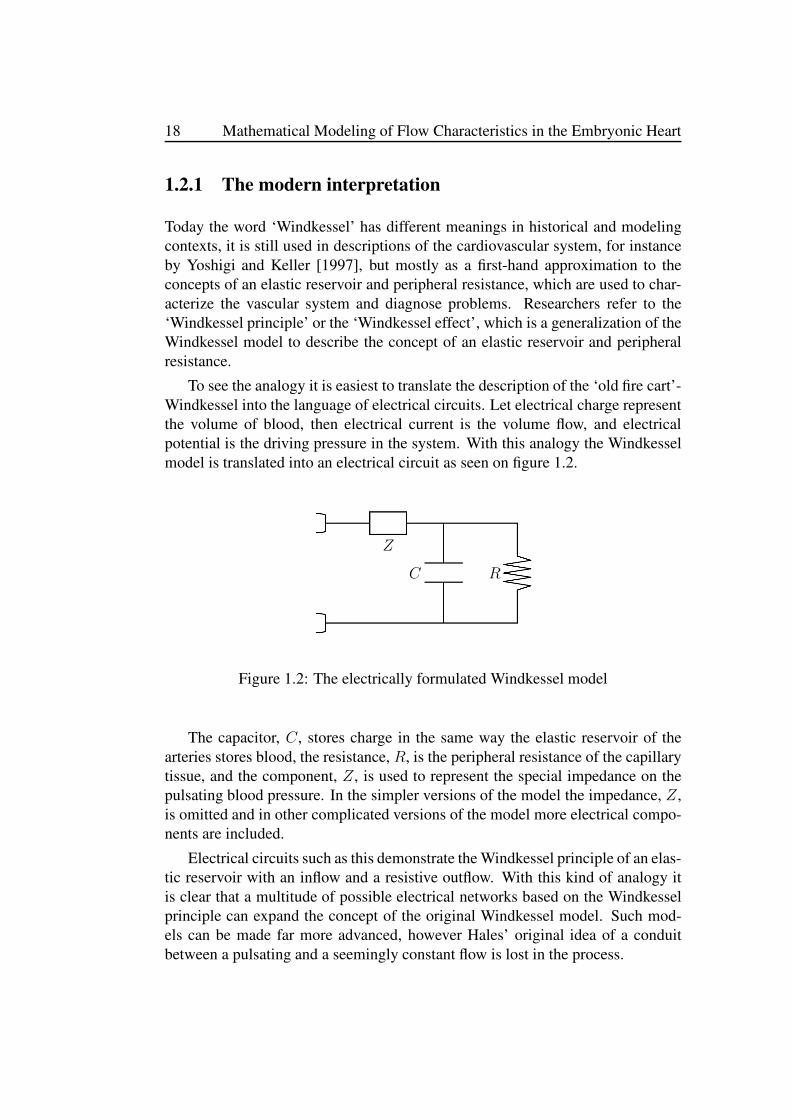
To see the analogy it is easiest to translate the description of the ‘old fire cart’-Windkessel into the language of electrical circuits. Let electrical charge representthe volume of blood, then electrical current is the volume flow, and electricalpotential is the driving pressure in the system. With this analogy the Windkesselmodel is translated into an electrical circuit as seen on figure 1.2.
Z
C R
Figure 1.2: The electrically formulated Windkessel model
The capacitor, C, stores charge in the same way the elastic reservoir of thearteries stores blood, the resistance, R, is the peripheral resistance of the capillarytissue, and the component, Z, is used to represent the special impedance on thepulsating blood pressure. In the simpler versions of the model the impedance, Z,is omitted and in other complicated versions of the model more electrical compo-nents are included.
Electrical circuits such as this demonstrate the Windkessel principle of an elas-tic reservoir with an inflow and a resistive outflow. With this kind of analogy itis clear that a multitude of possible electrical networks based on the Windkesselprinciple can expand the concept of the original Windkessel model. Such mod-els can be made far more advanced, however Hales’ original idea of a conduitbetween a pulsating and a seemingly constant flow is lost in the process.
Chapter 1: Introduction 19
1.2.2 The transmission line
An example of the expansion of the Windkessel principle through electrical net-works comes with the transmission line, which will be of importance for the mod-eling in chapter 4.
Expansions of the Windkessel principle via the electrical network analogue re-quires a specific interpretation of the included electrical elements in the model. Soto formulate the idea of the transmission line as a plausible model for the cardio-vascular system take as starting point the main argument against the Windkesselmodel that it leaves no possibility for pressure wave propagation in the system.
With the Windkessel principle the capacitor is considered as an elastic con-tainer for the volume of blood in the entire arterial system, but a capacitor couldequally describe a single arterial section. In this case the capacitance and resis-tance of the electrically formulated Windkessel model is applied to only a smallsection of arteries instead of the entire arterial tree.
The capacitance, C, of the model describes the (inverse) compliance of theelastic arterial wall and the resistance, R, models the resistance to flow out ofthe arterial section. Both of these will depend on the physical properties of theparticular section; radius, wall thickness, elasticity, length etc.
Consider the idea that several arterial sections are modeled one after the other:The continuity equation states that whatever flows out of one section must be theinflow to the next, in this way a chain of Windkessel models is achieved.
Additionally the pulsating pressure waves and pulsating volume flow produceaccelerating and decelerating velocities in the liquid, and for this, inertial effectsof the mass of blood inside the arteries are of great importance. Inertia of massis conveniently described with an inductance, L, in the electrical analogue, it isplaced in serial connection with the resistance since both inertia and flow resis-tance reacts to the displacement of the same amount of blood.
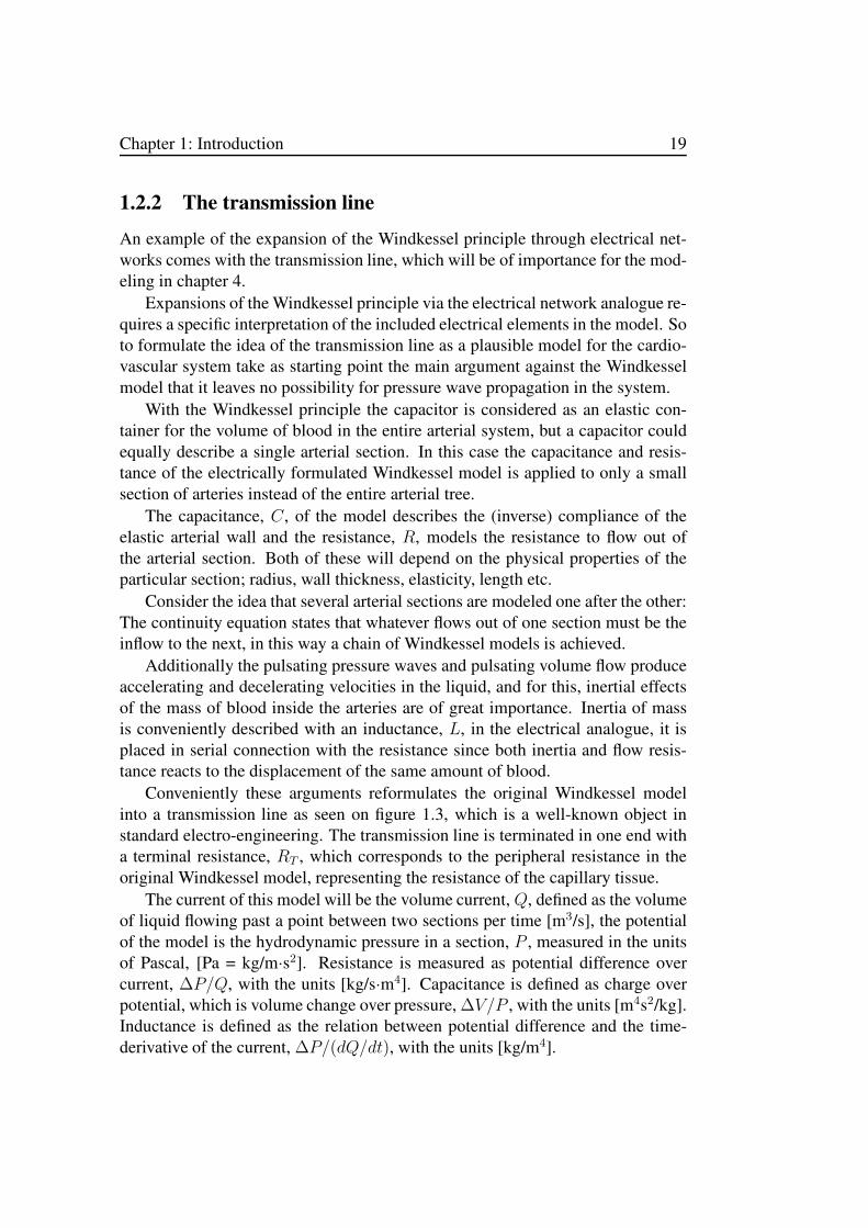
Conveniently these arguments reformulates the original Windkessel modelinto a transmission line as seen on figure 1.3, which is a well-known object instandard electro-engineering. The transmission line is terminated in one end witha terminal resistance, RT , which corresponds to the peripheral resistance in theoriginal Windkessel model, representing the resistance of the capillary tissue.
The current of this model will be the volume current, Q, defined as the volumeof liquid flowing past a point between two sections per time [m3/s], the potentialof the model is the hydrodynamic pressure in a section, P , measured in the unitsof Pascal, [Pa = kg/m·s2]. Resistance is measured as potential difference overcurrent, ∆P/Q, with the units [kg/s·m4]. Capacitance is defined as charge overpotential, which is volume change over pressure, ∆V/P , with the units [m4s2/kg].Inductance is defined as the relation between potential difference and the time-derivative of the current, ∆P/(dQ/dt), with the units [kg/m4].

20 Mathematical Modeling of Flow Characteristics in the Embryonic Heart
L1 R1
C1
L2 R2
C2
Ln Rn
Cn RT
Figure 1.3: The transmission line as an expansion from the Windkessel principle.
To complete this electrical analogue model the functions for resistance, capac-itance and inductance must be defined, which will not be attempted here as thatrequires further interpretation of the physiological phenomena.
1.2.3 The energy bond model
The transmission line is the first step in a generalization of the Windkessel prin-ciple, which will make it applicable to model the pulsating flow and pressure inan elastic tube. Through construction of chains of transmission lines it is possibleto construct large network models of the cardiovascular system, see for instance[Rideout, 1991].
When defining the resistance, capacitance and inductance of the transmissionline it will be clear that the elements of the model are non-linear and interrelated.In an attempt to explicitly describe the non-linear relations a group of physicistslead by Peder Voetmann Christiansen and Niels Boye Olsen from Roskilde Uni-versity in the 1980ies constructed an expansion to the transmission line. Themodel they built is reported and validated for blood flow in aorta as a students’project by Nørgaard et al. [1993], and later it is mentioned very briefly in a paperby Larsen et al. [2006].
The model is included in the first part of the modeling in chapter 4, it takesits start in the transmission line, and through the definition of the functions ofthe electrical elements it is naturally expanded. The model employs the advancedtechnique of energy bond formalism to expand the electrical network in figure 1.3.
Energy bond technique is a generalization of electrical analogue technique thatuse the same definitions as in electrical circuits but applies another diagram tech-nique that ensures that the implicit assumptions of electrical circuits are explicitlyreflected in the energy bond graphs. The rules and graphs of the energy bondtechnique are constructed to reflect physical consistency, as such the energy bondtechnique has more modeling potential than electrical networks.

Chapter 1: Introduction 21
One advantage of the energy bond technique is the way that models can beconstructed in stepwise order, and subsequently tested and expanded. The en-ergy bond technique makes the construction of mathematical models into build-ing blocks that can be added on top of each other, investigated or removed oneat a time. This is in contrast to other mathematical methods, for instance differ-ential equations, which are constructed from a set of assumptions that yield a setof equations to be solved; if there is a small change of assumptions a whole newmodel needs to be derived. If there is a small change of assumptions in an energybond model, single elements can be removed or changed as desired.


Chapter 2
The Embryonic Heart
The pumping embryonic heart has fascinated scientists for more than two thou-sand years, visible on top of the yolk as a tiny red spot that seems to pulsatein color. Aristotle who made the first documented observations of the pulsatingheart described it as “a speck of blood, in the white of the egg. This point beatsand moves as though endowed with life. . . ” [Aristotle., Historia Animalum BookVI 3].
Since the time of Aristotle generations of scientists have stared at the jumpingpoint, fascinated by its frailty and its meaning for development of new life. Forinstance a quote by William Harvey from his time as a student under Fabriciusof Aquapendente in Padua, years before his discovery of the circulatory system,illustrates this fascination and possibly the influence the embryonic heart mayhave had on the scientific history of medicine:
“I have seen the first rudiments of the chick as a little cloud in thehen’s egg about the fourth or fifth day of incubation, with the shellremoved and the egg placed in clear warm water. In the center ofthe cloud there was a throbbing point of blood, so trifling that it dis-appeared on contraction and was lost to sight, while on relaxationit appeared again like a red pin-point. Throbbing between existenceand non-existence, now visible, now invisible, it was the beginning oflife.”
- William Harvey circa 1600 [Gibson, 1978].
It was however not until the 1800th century when the motion of the speckof blood was correctly interpreted as the mechanical pumping of the embryonicheart by means of muscular contraction. One of the important researchers in thisdiscovery was Albrecht von Haller who in 1758 made a description of the contrac-tion pattern of the heart that led later scientists to formulate the peristaltic theoryof pumping for the embryonic heart [Männer et al., 2010].
23

24 Mathematical Modeling of Flow Characteristics in the Embryonic Heart
Having realized the muscular contractions of the embryonic heart scientistsbegan to discuss the origin of the contractions. Some held the belief that con-tractions were motivated externally via the nervous system while others believedin a local stimulation. In the end the intrinsic theory seemed to get the upperhand as it was possible to detect a contraction wave going from the venous end ofthe heart to the atrium and onwards to the ventricle, furthermore the contractionwas preceded by distension of the heart wall, which was seen as a local stimulusto contraction. Thus the intrinsic and peristaltic theories appeared to fit together[Männer et al., 2010].
Later still the peristaltic theory ran into problems as it was for instance dis-covered by Johnstone in 1925 that at the very early stages of the embryonic de-velopment only the ventricle shows contractions [Männer et al., 2008]. Scien-tists instead began to focus on the structure and genesis of the embryonic heart;the existence of cardiac jelly was discovered by Davis in 1924 and later in 1948Alexander Barry proved its importance for a peristaltic pumping function of theembryonic heart [Barry, 1948].
As such the history of the embryonic chick heart is as much a history of imag-ing techniques. In the early days of Aristotle and William Harvey the chick em-bryo was observed with the eye or a magnifying glass at best and described as atiny speck of blood. With the invention of the microscope by Anton van Leeuwen-hoek in the 17th century it was possible to better observe the heart, and shortlythereafter its tubular nature and contraction pattern was recognized. The resolu-tion of microscopy has steadily increased and with the invention of the electronmicroscope in the 1930ies impressive images could be made of the cell structureof the heart. Movie techniques and modern day optics have further improved thepossibilities in envisioning the embryonic heart.
2.1 Hamburger and Hamilton stages
The chick embryo has been a research specimen for embryological research forseveral hundred years, as it is both simple to obtain chicken eggs and simple to getto the embryo, but in 1951 research in the chick embryo was made even easier.This was the year when Viktor Hamburger and Howard L. Hamilton publishedtheir report detailing the embryonic chick development in 46 stages of the 21 daysincubation period [Hamburger and Hamilton, 1951].
The work by Hamburger and Hamilton characterizes the embryonic devel-opment of the chick from distinguishing diagnostics in the embryo such as thelength of the beak, tail, wings or legs, the size and color of the eye, or the numberof somites, which are masses of mesoderm that form along the neural tube andeventually will become part of the backbone and adjoining muscles.

Chapter 2: The Embryonic Heart 25
By making diagnosis according to the characterizations by Hamburger andHamilton it is possible to determine and compare the exact development of thechick embryo through the identification of its Hamburger and Hamilton stage(commonly known as HH-stage). The identification of HH-stages has become theprimary way of diagnosing development of the chick embryo since Hamburgerand Hamilton [1951]. Before their report the development of the embryo was typ-ically characterized according to days and hours of incubation, see for instance[Barry, 1948], but as embryonic development may vary this method was unreli-able.
In relation to the overall development of the chick embryo Martinsen [2005]has made a detailed description applying the HH-stages specifically to the embry-onic heart (some medical terms are used here and explained later in the text):
HH-stage 6-7 The primary heart tube starts to form.
HH-stage 8-9 First morphological manifestation of the straight heart tube.
HH-stage 10-11 The heart tube is still open ended, onset of the morphologicalprocedure ‘cardiac looping’, the heart starts to beat.
HH-stage 12-13 The heart tube is a closed system, cardiac looping has com-pleted its dextral looping phase, early formation of endocardial cushions,the beating of the heart is stable, flow is observed.
HH-stage 14-15 Cardiac looping forms the s-shaped heart, onset of the epicardialcell diffusion.
HH-stage 16 Onset of atrial septation, clear atrioventricular and outflow tractcushions.
HH-stage 17-18 Formation of the s-shaped heart complete, epicardial mantlebegins to form over the myocardium, onset of trabeculation of the ventricle.
HH-stage 19-20 Formation of a primitive interventricular septum, extensive tra-beculation of the ventricle, epicardium covers the inner curvature of theheart.
HH-stage 21-23 Two pairs of endocardial cushions are formed at the outflowtract, valve formation in the atrioventricular cushion begins, epicardial cellspenetrate into the myocardium.
HH-stage 24 Cardiac looping completed with the mature s-shaped heart, onsetof cardiac septation, loss of original tubular character.
HH-stage 25-46 Cardiac septation transforms the embryonic heart to the maturefour-chambered heart.

26 Mathematical Modeling of Flow Characteristics in the Embryonic Heart
The description of the embryonic heart development details how the heartgrows from the heart tube to the four-chambered heart, many morphological changeshappen during this process but only the important ones for this thesis are ac-counted for here: During HH-stage 15 and onwards epicardium starts to form,this is outer protective layer of the mature heart that will form on top of the my-ocardial layer and increase its stiffness. The formation of endocardial cushionscreates cushions of soft gelatinous material at select positions in the heart tube,and eventually they will grow into the heart valves. The process of cardiac loop-ing is detailed below. The processes of trabeculation and cardiac septation areboth processes that will undo the morphology of the tubular heart and transformit to the four-chambered heart, and already from HH-stage 18 the heart tube willstart to include a complicated mesh of fibers at its walls.
The embryonic heart starts beating at HH-stage 10 as the first functional organin the embryo [Männer et al., 2009]. This probably happens in conjunction withthe growing of the embryo, which at this stage may have attained a size above thethreshold where cell and nutrient transport may no longer be effectively suppliedby diffusion. In human cells diffusion lengths range up to about 1 mm [Olufsen,1998], which fits well with this hypothesis.
From this analysis of the HH-stages of the embryonic heart, it is clear thatstages before HH-stage 10 are uninteresting for the modeling, because there is noheart beat, while stages after HH-stages 18 may still be interesting but increasinglyharder to model using the models in this thesis due to ventricular trabeculation.
2.2 Cardiac looping
Cardiac morphogenesis has been a research field for more than 300 years, whilethe knowledge that the embryonic heart actually starts as a simple tube is probablyolder still. The first record of the fact that the heart tube shows the morphology ofa loop was made in 1758 by Albrecht von Haller, while Bradley M. Patten in 1922introduced the concept that the formation of the heart loop was a distinct processin the development of the heart, effectively coining the term ‘cardiac looping’[Männer, 2000].
Cardiac looping has seen immense interest from developmental biologists be-cause the looping of the heart tube and concurrent rightward rotation is the earliestleft-right asymmetry in the developing vertebrate embryo, and also data from ex-perimental embryology seem to support the idea that abnormal cardiac loopingmay be responsible for the development of malformed hearts [Männer, 2000].
Chapter 2: The Embryonic Heart 27
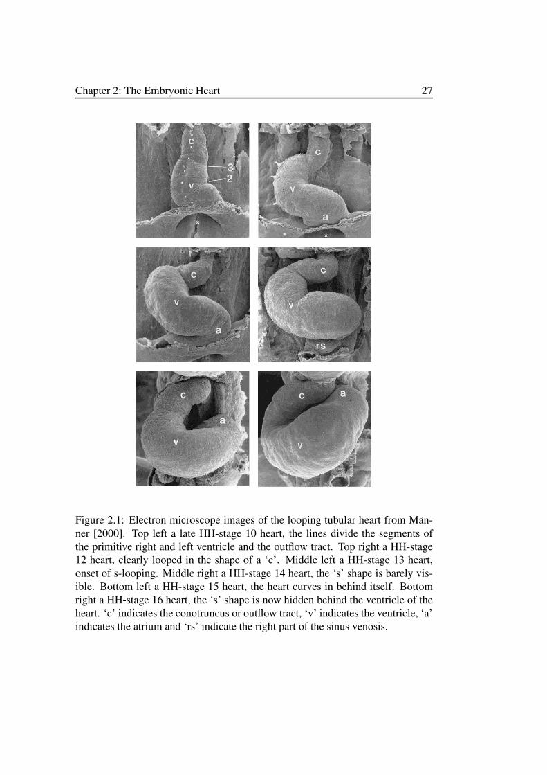
Figure 2.1: Electron microscope images of the looping tubular heart from Män-ner [2000]. Top left a late HH-stage 10 heart, the lines divide the segments ofthe primitive right and left ventricle and the outflow tract. Top right a HH-stage12 heart, clearly looped in the shape of a ‘c’. Middle left a HH-stage 13 heart,onset of s-looping. Middle right a HH-stage 14 heart, the ‘s’ shape is barely vis-ible. Bottom left a HH-stage 15 heart, the heart curves in behind itself. Bottomright a HH-stage 16 heart, the ‘s’ shape is now hidden behind the ventricle of theheart. ‘c’ indicates the conotruncus or outflow tract, ‘v’ indicates the ventricle, ‘a’indicates the atrium and ‘rs’ indicate the right part of the sinus venosis.
28 Mathematical Modeling of Flow Characteristics in the Embryonic Heart
From the formation of the straight heart tube at the very early stages of theembryo, cardiac looping is the process that transforms the heart into a fully devel-oped s-shaped curved heart tube at the onset of cardiac septation and the formationof the four chambered heart, this development is said to go through three phases:dextral looping, formation of the primitive s-loop, and formation of the mature s-loop [Männer, 2004]. A series of electron microscope images from Männer [2000]depicting the looping heart in the stages of interest for the modeling in the thesisis visible on figure 2.1.
At the beginning of cardiac looping around HH-stage 9 the embryonic hearthas grown from nothing to a straight and almost symmetric tube (in the so calledprelooping phase) oriented along the ventral midline (central) of the embryo. Theheart tube consist of the early stages of the future ventricles connected to two ve-nous inlets at its lower end and an arterial outlet at its upper end, which quicklyseparates into two main arteries destined to become the aorta and pulmonary arteryduring later stages of development. During the growth of the embryonic heart inthe following phases additional ‘cardiac segments’ (atrioventricular canal, com-mon atrium, systemic venous sinus, outflow tract) are added to the heart tubefrom its upper and lower end respectively, though the tube remains principallyundivided and valveless [Männer, 2008].
Dextral looping is the process that transforms the straight heart tube to a c-shaped curved heart tube. The process starts at HH-stage 9-10 and ends at HH-stage 12. It was previously believed that dextral looping occurred as a result ofa spatially confined growth of the heart tube causing the tube to bulge, though itwas not possible to explain why the tube would always bulge rightwards. Recentresearch has however revealed that the looping of the heart is comprised of alengthwise growth and a consequently ventral bending (towards the front of theembryo) combined with a rightward rotation of the upper part of the tube alongthe craniocaudal axis (the head-to-toe axis) forcing a counterclockwise rotation ofthe tube to the right [Männer, 2004].
Following dextral looping the next process transforms the c-shaped curvedheart tube into an s-shaped looping heart with the onset at HH-stage 13 until HH-stage 18, with a clear s-shaped loop visible already at HH-stage 14. This processis primarily characterized by the shortening of the distance between the primitiveoutflow tract at the upper end and the primitive atria at the lower end of the hearttube supposedly combined with a leftward rotation of the lower end of the tube[Männer, 2004].
The final process of maturing the s-shaped loop occurs from HH-stage 19 untilHH-stage 24, at which the tubular heart effectively ceases to exist. This processis mainly characterized by an immense growing of the heart and the shift of theoutflow tract and the atria to their final positions [Männer, 2000].

Chapter 2: The Embryonic Heart 29
All the while these processes transform the straight heart tube into the loopingheart, the heart is beating. Starting around early HH-stage 10 the heart beats ir-regularly and slowly but by the end of stage 10 a clear heart rhythm is presentand during later stages the frequency increase [Castenholz and Flórez-Cossio,1972], blood flow can be detected as early as HH-stage 11 [Castenholz and Flórez-Cossio, 1972] and at stage 12 a peristaltic wavelike contraction pattern can beobserved along the length of the heart tube from the atrium to the outflow tract[Taber, 2006a].
Thus it is clear that the interesting stages for the modeling will be HH-stage 10when the heart starts beating but before the completion of the c-shaped loop, HH-stage 12 with a complete c-shaped heart loop and a complete contraction waverhythm, HH-stage 14 with an early s-shaped heart loop, and HH-stage 16 witha fully s-shaped heart including all the heart segments of the looping heart, seefigure 2.1. These four stages will be the ones in question during the model setupprocess described in chapter 7.
2.3 Beating of the looping heart
At HH-stage 10 the tubular embryonic heart starts beating. At first the beatingis irregular, slow and only periodic in short intervals but late during HH-stage10 a stable periodic rhythm is formed [Castenholz and Flórez-Cossio, 1972], stillthe contraction pattern is primitive and only in the subsequent stages will that beimproved [Martinsen, 2005].
To achieve propulsion of blood the tubular heart is a layered structure con-sisting of an inner layer, the endocardium, and an outer layer, the myocardium(before the onset of epicardial formation), and in between the two resides a gelati-nous material known as cardiac jelly. The myocardium is a relatively thick layerthat contains the contractile muscular fibers of the heart tube known as sacomeres,it has no specific fiber architecture and the muscle fibers are distributed rather ran-domly Lin and Taber [1994]. The endocardium is a thin one-cell thick layer withcomposition similar to the myocardium Lin and Taber [1994]. It separates thecardiac jelly and the inner lumen of the heart, and it appears as if the function ofthe endocardium is to shield the blood inside the heart tube.
The cardiac jelly is an extracellular gelatinous material that contain radiallyoriented fibers, less at the early HH-stages more at the later stages before trabec-ulation. It is considerably softer than the other layers but may show existenceof anisotropy [Zamir and Taber, 2004]. Following a peristaltic pumping principleBarry [1948] proved the essential function of the cardiac jelly to achieve occlusionof the lumen of the heart tube and hence to propagate liquid in the tube.
30 Mathematical Modeling of Flow Characteristics in the Embryonic Heart
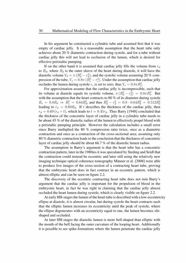
In his argument he constructed a cylindric tube and assumed first that it wasempty of cardiac jelly. It is a reasonable assumption that the heart tube onlyachieves about 20 % diametric contraction during systole, and for a tube withoutcardiac jelly this will not lead to occlusion of the lumen, which is desired foreffective peristaltic pumping.
If on the other hand it is assumed that cardiac jelly fills the volume from rdto Rd, where Rd is the outer sleeve of the heart during diastole, it will have thediastolic volume Vd = π (R2
d − r2d), and the systolic volume assuming 20 % com-pression of the tube, Vs = 0.8π (R2
s − r2s). Under the assumption that cardiac jellyoccludes the lumen during systole rs is set to zero, thus Vs = 0.8πR2
s.For approximation assume that the cardiac jelly is incompressible, such that
its volume at diastole equals its systolic volume, π (R2d − r2d) = 0.8πR2
s. Butwith the assumption that the heart contracts to 80 % of its diameter during systoleRs = 0.8Rd ⇒ R2
s = 0.64R2d, and thus R2
d − r2d = 0.8 · 0.64R2d = 0.512R2
d
leading to rd = 0.69Rd. If t describes the thickness of the cardiac jelly, thenrd = 0.69 (rd + t), which leads to t = 0.45rd. Thus Barry [1948] concluded thatthe thickness of the concentric layer of cardiac jelly in a cylindric tube needs tobe about 45 % of the diastolic radius of the lumen to effectively propel blood witha peristaltic pumping principle. However the calculation includes a small errorsince Barry multiplied the 80 % compression ratio twice, once as a diametriccontraction and once as a contraction of the cross-sectional area; assuming only80 % diametric contraction leads to the conclusion that the thickness of concentriclayer of cardiac jelly should be about 66.7 % of the diastolic lumen radius.
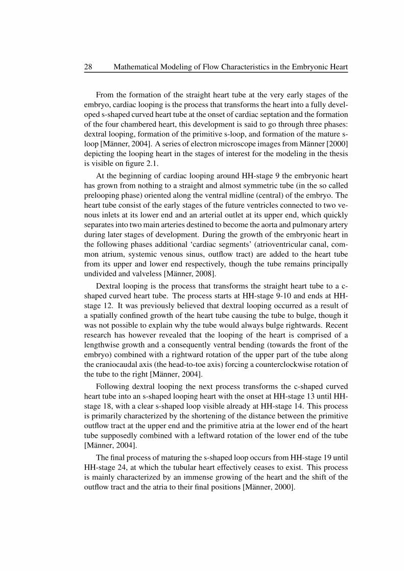
The assumption in Barry’s argument is that the heart tube has a concentriccontraction pattern, later in the 1980ies it was speculated by Steding and Seidl thatthe contraction could instead be eccentric and later still using the relatively newimaging technique optical coherence tomography Männer et al. [2008] were ableto produce live images of the cross-section of a contracting heart tube, provingthat the embryonic heart does in fact contract in an eccentric pattern, which isalmost elliptic and can be seen on figure 2.2.
The discovery of the eccentric contracting heart tube does not ruin Barry’sargument that the cardiac jelly is important for the propulsion of blood in theembryonic heart, in fact he was right in claiming that the cardiac jelly almostoccluded the heart lumen during systole, which is clearly visible on figure 2.2.
At early HH-stages the lumen of the heart tube is described with a low-eccentricityellipse at diastole, it is almost circular, but during systole the heart contracts suchthat the elliptic lumen increases its eccentricity until the peak of systole, wherethe ellipse degenerates with an eccentricity equal to one, the lumen becomes slit-shaped and occluded.
At later HH-stages the diastolic lumen is more bell-shaped than elliptic withthe mouth of the bell facing the outer curvature of the looping heart. Additionallyit is possible to see spike-formations where the lumen penetrate the cardiac jelly

Chapter 2: The Embryonic Heart 31
End-diastole Mid-systole End-systole Mid-diastole
Figure 2.2: OCT images of the layered cross-sections of the beating heart fromMänner et al. [2008]. It is clearly seen how the inner endocardial layer contractsalmost elliptically while the outer myocardial layer contracts in an almost concen-tric manner.
and reach out to the myocardium of the heart tube. The lumen is not always com-pletely occluded during systole, yet the contraction pattern is still clearly eccentric[Männer et al., 2009].
Meanwhile the outer sleeve of the heart, the myocardium, contracts in an al-most concentric manner, though it is proved by Männer et al. [2009] that the con-traction is slightly eccentric from HH-stage 14 to 17 and possibly also earlier. Theapproximate concentric contraction of the myocardial sleeve seems to confirm theassumption by Barry that the relatively little outer contraction of the heart tubemakes the cardiac jelly fill up the entire volume inside the heart tube, essentiallythrough incompressibility.

32 Mathematical Modeling of Flow Characteristics in the Embryonic Heart
The construction of the elliptic layer of cardiac jelly in the heart tube comesas a consequence of the generation of the tubular heart, as it grows from twoheart-forming fields on either side of the sagittal plane of the embryo (the cross-sectional plane that divides left and right in the body) in a bilateral process duringHH-stages 6 and 7, and at HH-stage 8 the two halves get fused together alongthe major axis of the later elliptic cross-section [Martinsen, 2005]. An interestingquestion is if there are other reasons that the heart lumen is elliptic apart from itsgenesis.
One advantage of eccentric contraction seems to be the strain endured by cellsin the endocardial inner layer of the heart wall. In hypothetical heart tubes withconcentric contraction, like the one suggested by Barry, the endocardial cells un-dergo severe strains from diastole to end-systole, while heart tubes with the ob-served eccentric deformation pattern expose the endocardial cells to much lighterdimensional changes. It may be that the observed eccentric contraction is made tominimize stress in the walls of the heart tube [Männer et al., 2008].
Concerning peristaltic transport of fluid it has been proven for technical casesthat tubes of elliptic cross-section have a higher mechanical efficiency of peri-staltic pumping compared to tubes of circular cross-section, and similar resultshave been achieved for simple models of the tubular embryonic heart under as-sumption of peristaltic pumping [Männer et al., 2008]. Thus evidence suggestthat the tubular heart is made to optimize blood pumping capabilities.
2.3.1 Optical coherence tomography
Optical Coherence Tomography (OCT) is an echo-based imaging modality thatmeasures the time-of-flight of back-reflected light using low-coherence interfer-ometry. OCT use a near-infrared light source and measures the light scatteringand reflection of light relative to light traveling a known reference path inside theOCT apparatus. The system obtains images with a resolution of 10 to 30 µm withdepth penetrations of a few millimeters (typically 2-3 mm), deep enough to scanthe live pumping heart of the chick embryo [Yelbuz et al., 2002].
The imaging technique of OCT is more or less the same as in the more com-monly applied ultrasound technique; a single two-dimensional image scan (knownas a B-scan) consists of several thousand one-dimensional scans (A-scans) as theprobe beam is laterally scanned across the sample. Alternatively A-scans can bemade sequentially at a stationary location to show time-development in the socalled M-mode images. Naturally sample speed is essential for this technique; ahigher frequency means a higher number of A-scans per second, which can betranslated into a better M-mode resolution or a higher number of A-scans per B-scan. A-scan resolution is another important factor in this imaging technique; atypical A-scan beam has a width of 10 to 20 µm in both axial and lateral dimen-sion, which defines the resolution of B-scan images.

Chapter 2: The Embryonic Heart 33
OCT was introduced in 1991 and has been thoroughly used in the imagingof semi-transparent tissues (such as the chick embryo) or highly light-scatteringtissues (such as the retina of the eye) in its twenty year lifetime. However thetechniques used in imaging of chick embryos is no more than ten years old [Yelbuzet al., 2002]. Some of the newest approaches to the technique is the combinationwith Doppler theory to achieve dimensional as well as dynamical information[Davis et al., 2009] and the combination of images to achieve 3D (or even 4D)images [Liu et al., 2009] as well as a general A-scan resolution and increase insampling frequency of the OCT equipment.
2.4 Peristaltic pumping vs. the Liebau effect
Following the discovery of muscular contractions of the embryonic heart it wasquickly discovered by Albrecht von Haller in 1758 that a wavelike contractionpattern was visible from the venous end of the heart tube towards the arterialend, and that this contraction wave was preceded by a short distension of thewall of the tube given by the compliant reaction to the inflow of blood. Theseobservations made von Haller conclude that the heart contraction reacted to alocal pressure stimulus, which fit well together with a peristaltic pumping theoryof blood propulsion [Männer et al., 2010].
Peristaltic pumping was already recognized by scientists as the pumping prin-ciple of the gut and the ureter, and it was conspicuous to believe the same principlewould govern the pumping of blood as well. During the 19th century a long rangeof scientists succeeded in constructing a convincing description of the embryonicheart as a peristaltic pumping mechanism that responded to intrinsic stimuli toproduce a stable propulsion of blood out through the vascular system and eventhe four-chambered heart was described as peristaltic by Gaskell in 1883 [Männeret al., 2010].
This reveals that in the 18th and 19th century peristaltic pumping was definedin a much broader sense than today. Modern peristaltic pumping can be envisionedas a sliding contraction of the heart tube, or in some cases a sequential contraction,such that the liquid is pushed forward by the contraction wave. From this followsthat a peristaltic contraction wave requires a certain length of contractile tube towork.
As such it was contradicting to the peristaltic hypothesis when Johnstone dis-covered that the HH-stage 10 heart only contracts its ventricle in an almost uni-form manner [Männer et al., 2008]. But already the peristaltic pumping theorywas in a state of crisis. During the 19th and especially the 20th century peri-staltic fluid transport became a more specialized mechanical principle as engi-neers, physicists and mathematicians achieved interest in this phenomenon, and

34 Mathematical Modeling of Flow Characteristics in the Embryonic Heart
at the same time physicians made much more specific definitions of the biologicalperistalsis of the gut and ureter, so by the beginning of the 20th century the em-bryonic heart could hardly be described as a peristaltic pump any longer [Männeret al., 2010].
And then in 1954 a new pumping theory was introduced. Gerhart Liebau pro-posed a pumping principle based on an active pumping action at a single pointon the tube creating a pulsating pressure wave that when interacting with the im-pedance of the heart and vascular system would create a flow. Liebau was mostlyinterested in the mature heart and he explained his ideas by construction of sim-ple mechanical pumping systems that did not catch the interest of embryologists,but he did in fact speculate about the applicability of his pumping principle as analternative to the peristaltic pumping in the embryonic heart [Liebau, 1955].
Liebau’s theories mostly caught the interest of mathematicians and physicistsand for many years after its introduction the so called Liebau effect was mostlyconsidered a phenomenon of relatively simple experimental setups in fluid me-chanics. It was speculated that the Liebau effect could have influence on theembryonic heart but it was not until a research group from the California Insti-tute of Technology lead by Farouhar, Gharib and Hickerson in 2006 decided toinvestigate whether the embryonic zebrafish heart might work as a Liebau pumpthat Liebau theory was actually considered as a viable alternative to the peristalticpumping theory [Männer et al., 2010].
The Liebau effect has proven to be a competing theory to the peristaltic pumpin relation to the embryonic heart, and it has recently caught interest with manyembryologists. It is however not a complete alternative, just like the peristalticpump the embryonic heart demonstrates behavior that can not be explained withthe simple Liebau effect. In a comparison between the two pumping principlesMänner et al. [2010] compiles a list of characteristics for the simple technicalcase of a peristaltic pump:
Characteristics of the technical peristaltic pump:
The pump is a positive displacement pump that generate flow bypushing the liquid forward.
The pump has non-stationary sites of active compression that movesalong the length of a flexible tube.
Movement of active compression sites is seen as a unidirectionallypropagating compression wave.
The flow generated is continuous.
No structurally fixed direction of net flow; flow direction dependson the direction of the compression waves.
Chapter 2: The Embryonic Heart 35
The generated flow velocity corresponds to the speed of the com-pression waves.
There is a linear relation between compression wave frequency andflow rate.
It should be noted that these are characteristics of the technical peristalticpumps used in engineering and industry. In biology there is at least one exampleof a peristaltic pump that works differently than the technical pump, the gastricemptying of the stomach produce flow velocities far higher than the correspondingcompression wave. Furthermore recent computational modeling demonstrate thatperistaltic heart tubes can generate pulsatile flow as a consequence of the endocar-dial cushions at the inflow and outflow regions of the tube [Männer et al., 2010].Thus it is important to distinguish between technical and biological peristalticpumps, as the latter is able to demonstrate characteristics not normally describedwith technical peristalsis.
Correspondingly the list for the characteristics of the Liebau effect by Männeret al. [2010] is compiled for a simple technical Liebau pump involving only asingle compression site, despite the fact that a sequence of compressions is likelymore appropriate for the embryonic heart [Liebau, 1955]:
Characteristics of the simple Liebau pump:
The pumping tube must have a flexible wall of finite length.
There has to be a mismatch of impedance right and left in relation tothe pumping site (preferably at the ends of the flexible tube).
The pump includes only a single stationary site of active compres-sion.
The active compression site must be at an asymmetric position alongthe tube.
The generated flow is pulsatile.
No structurally fixed direction of net flow; flow direction dependson frequency.
Generation of bidirectional elastic waves traveling along the passivewalls of the tube (both upstream and downstream).
The flow velocity can exceed the speed of the traveling elastic waves.
There is a non-linear relationship between compression frequencyand flow rate.

36 Mathematical Modeling of Flow Characteristics in the Embryonic Heart
Both pumping principles demonstrate valveless pumping action and as suchthere is no structural dependency (for instance by valves) of the direction or mag-nitude of the generated flow. For the peristaltic pump the flow follows the directionof the compression waves and is linear dependent on compression wave speed andfrequency. For the Liebau pump the flow depends on the frequency of stationarycompressions and their position in relation to the distribution of impedance in thetube, the dependency is non-linear and at certain frequencies the flow may changedirection.
Generally the embryonic heart demonstrate what appears to be a wave ofcontractions along its length, which has prompted the peristaltic hypothesis. Ithas been proved that these contractions can not be generated by passive com-pliance to a strong singular compression function, and furthermore studies showthat when the different cardiac segments are physically isolated they still utilizethe same contraction pattern indicating active compression in all segments of theheart [Männer et al., 2010], which all support the peristaltic theory. On the otherhand researchers have discovered embryonic hearts in fish and lower vertebratethat only employ a single contraction site, and at the same time it is reportedthat the contraction wave in higher vertebrate embryos (such as the chick) hasa ‘kickstart’ contraction of the atrium while the rest if the contraction pattern ismore steady [Männer et al., 2010], such discoveries seem to support a complicatedLiebau mechanism.
It has been argued how the influence of cardiac jelly and the elliptic cross-section optimize the embryonic heart for peristaltic transport, but in fact it canalso be hypothesized that cardiac jelly may have a high influence on fluid transportfollowing the Liebau principle via its elastic nature, such that it may amplify theelastic waves responsible for the Liebau effect, regardless that lumen occlusion isnot normally observed in standard technical Liebau pumps [Männer et al., 2010].
The two pumping theories have both merits and flaws in relation to the mea-sured characteristics of the heart, but none are strong enough to completely ex-clude the theory as a possible explanation of the pumping mechanism of the em-bryonic heart.
2.5 The questions about the embryonic heart
It is made clear how the embryonic heart starts its genesis as a looped multilayeredtube and begins beating contractions as soon as it is generated, at first the contrac-tions are simple and irregular but later a clear contraction wave or sequence ofcontractions is seen traveling the heart tube from the venous end over the atriumand ventricle to the outflow tract.

Chapter 2: The Embryonic Heart 37
The tubular heart is generated during HH-stage 9 and 10 as an almost straighttube, but in the subsequent stages the tube curves into a c-shaped tube at HH-stage 12 and an s-shaped tube from HH-stage 14 until HH-stage 24. This happenswhile the tube is also growing in length by adding new cardiac segments to theembryonic heart, in this way the tubular heart is fully formed at HH-stage 16, allthough at later stages the cardiac segments grow further. In the stages followingHH-stage 16 the processes of trabeculation and cardiac septation transforms themultilayered looping heart into the mature four-chambered heart. It is not knownif the morphology of the looping heart is only a process in forming the matureheart or if the looping has an influence to optimize flow conditions in the heart.
The tube is layered such that between the inner endocardial layer and the outermyocardial layer resides a layer of gelatinous material known as cardiac jelly. Thedistribution of cardiac jelly in the heart tube is eccentric, forming two cushions oneither side of the heart tube such that the inner lumen of the heart tube appearsalmost elliptic. It has been reasonably established that the cardiac jelly and theelliptic cross-section optimizes conditions for peristaltic pumping, but it is not yetknown if it will also have an increased effect on Liebau pumping.
Two hypothetic theories are suggested for the pumping mechanism of the tubu-lar heart: peristaltic pumping or the Liebau effect. Both theories have characteris-tics that seem to support or conflict with the observations of the embryonic heart,the question has recently been which of these are the correct description of pump-ing in the heart, but perhaps a more relevant question would be if they are mutuallyexclusive.


Chapter 3
Flow Theory
The embryonic chicken heart is a special case of bio-mathematical modeling ofblood flow, and the first step in the modeling procedure will be to recount some ofthe established theory on the area. The purpose of this chapter will be to presentsome of the fundamental concepts and theories, which will be used in the model-ing, at the while arguing why the embryonic heart can not be modeled solely fromthese basic principles.
The concepts and theories herein come from the classic fluid dynamics, whichshould be subdivided into aerodynamics, concerning compressible fluids, and hy-drodynamics, concerning incompressible fluids. Yet many researchers feel theneed to express that blood is a special kind of fluid that is bound to demon-strate non-Newtonian behavior and a complex compressibility, therefore they havecoined the term ‘hemodynamics’ for the special study of blood and the cardiovas-cular system [McDonald, 1968].
The three most important concepts here are the nature of the liquid, the elastictube walls and the pulsating flow and pressure. This may all be modeled withhydrodynamical theory as a first approximation, which will also be the startingpoint of this chapter but during the course of the chapter (and especially laterchapters) it should be clear that hydrodynamics will not be sufficient, which bothwarrants the models of chapter 4 and 6 as well as the name ‘hemodynamics’.
3.1 Basic properties of fluids
A fluid in physics is a continuous material medium that flows, this is in fact theone thing that distinguishes a fluid from a solid, in more specific terms, a fluidcannot maintain a shear stress for any length of time [Feynman et al., 1964, 40-1].Fluids are like any other material characterized by their mass density, ρ [kg/m3],while the special flow property of a fluid is characterized by the measure of theviscosity, η [1 Pa·s = 10 Poise], thicker liquids like honey move less easily thanfluids like air or water.
39

40 Mathematical Modeling of Flow Characteristics in the Embryonic Heart
A
A
d v(x)
v0
F
Figure 3.1: The typical model to illustrate viscosity. Imagine two parallel platesof equal area, A, with distance, d, between them. The plates move with speed, v0,relative to each other. The viscosity can then be found by measuring the force, F ,needed to maintain a constant velocity.
The measure of viscosity is usually explained by imagining two parallel platesof equal area, A, separated by a layer of fluid, one plate is held stationary and theother is moved parallel to the first with a slow constant speed, v0. See figure 3.1.The force, F , required to keep the plate moving will be proportional to the areaof the plates and to v0/d, where d is the distance between the plates. Thus theshear stress, F/A, induced on the liquid is proportional to v0/d, and the constantof proportionality is called the coefficient of viscosity,
F
A= η
v0d. (3.1)
Usually the viscosity is a fixed constant at all but the most extreme cases, forblood however it is a little different. The viscosity of blood have two known anom-alous properties typically referred to as the ‘low shear’ and ‘high shear’ effects;[Nichols and O’Rourke, 1998, p. 18]
Low shear effect: At low shear stress, the apparent viscosity of blood increasesmarkedly. It has been shown with almost certainty that flow may cease inthe presence of a very low measurable stress, implying that there is a ‘yieldstress’ under which blood is not a fluid.
High shear effect: In small tubes, the apparent viscosity of blood at high shearstress is smaller than it is in larger tubes. This effect begins to be detectablewith tubes of less than 1.0 mm internal diameter (i.e. about 100 times themajor diameter of red blood cells).
A fluid in classical physics is either Newtonian or non-Newtonian. A New-tonian fluid obeys a linear relationship between stress and velocity like the onedescribed in equation 3.1, which means a Newtonian fluid has a constant viscos-ity. Clearly the low shear and high shear effects make blood a non-Newtonianliquid, which in general will make the equations of motion for blood flow un-solvable. It is however commonly assumed that there is a large interval of shear
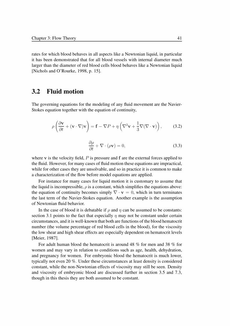
Chapter 3: Flow Theory 41
rates for which blood behaves in all aspects like a Newtonian liquid, in particularit has been demonstrated that for all blood vessels with internal diameter muchlarger than the diameter of red blood cells blood behaves like a Newtonian liquid[Nichols and O’Rourke, 1998, p. 15].
3.2 Fluid motion
The governing equations for the modeling of any fluid movement are the Navier-Stokes equation together with the equation of continuity,
ρ
(∂v
∂t+ (v · ∇)v
)= f −∇P + η
(∇2
v +1
3∇(∇ · v)
), (3.2)
∂ρ
∂t+∇ · (ρv) = 0, (3.3)
where v is the velocity field, P is pressure and f are the external forces applied tothe fluid. However, for many cases of fluid motion these equations are impractical,while for other cases they are unsolvable, and so in practice it is common to makea characterization of the flow before model equations are applied.
For instance for many cases for liquid motion it is customary to assume thatthe liquid is incompressible, ρ is a constant, which simplifies the equations above:the equation of continuity becomes simply ∇ · v = 0, which in turn terminatesthe last term of the Navier-Stokes equation. Another example is the assumptionof Newtonian fluid behavior.
In the case of blood it is debatable if ρ and η can be assumed to be constants:section 3.1 points to the fact that especially η may not be constant under certaincircumstances, and it is well-known that both are functions of the blood hematocritnumber (the volume percentage of red blood cells in the blood), for the viscositythe low shear and high shear effects are especially dependent on hematocrit levels[Meier, 1987].
For adult human blood the hematocrit is around 48 % for men and 38 % forwomen and may vary in relation to conditions such as age, health, dehydration,and pregnancy for women. For embryonic blood the hematocrit is much lower,typically not even 20 %. Under these circumstances at least density is consideredconstant, while the non-Newtonian effects of viscosity may still be seen. Densityand viscosity of embryonic blood are discussed further in section 3.5 and 7.3,though in this thesis they are both assumed to be constant.

42 Mathematical Modeling of Flow Characteristics in the Embryonic Heart
3.3 Laminar flow vs. turbulent flow
Another important characterization of fluid motion, which has become an impor-tant discussion in hemodynamic research, is the determination of the nature of theflow.
General hydrodynamics defines the concepts of laminar and turbulent flow: Ifthere exist an ordering of layers inside the fluid such that each layer, beginningwith the outer layer along the boundaries of the liquid, have a uniform velocitythe flow is said to be laminar, otherwise it is turbulent.
In ordinary hydrodynamic theory the question of laminar versus turbulent flowcan usually be determined by referring to the Reynolds number. This numberis basically a comparison of the magnitude of two terms of the Navier-Stokesequation, the advective term of velocity change, (v ·∇)v, and the viscous term ofvelocity change, ν∇2
v, where ν = η/ρ is the kinematic viscosity.These two terms govern two properties of all kinds of flow, inertia and viscos-
ity. Inertia attempts to continue the motion of a fluid once it is started whereasviscosity acts as a brake. If inertia is dominant the flow is said to be ideal, it iscustom to leave out the viscous term from the Navier-Stokes equation in thesecases. If viscosity is dominant the flow is usually known as creeping flow and theadvective term can be omitted. [Lautrup, 2005, p. 237]
To get a measure of these two terms assume that for a certain region of the fluidthe velocity is of a typical size, |v| ≈ U , and that it changes by a similar amountover a region of size L. The order of magnitude of the first-order spatial derivativeof the velocity will then be |∇v| ≈ U/L and the second-order derivative willbe of magnitude |∇2
v| ≈ U/L2. Consequently the construction of the Reynoldsnumber will be,
Re =|(v · ∇)v||ν∇2v| ≈ U2/L
νU/L2=ρUL
η. (3.4)
For small values of the Reynolds number the flow is laminar and orderly, hencecreeping flow (Re ≪ 1) is always laminar. For larger values, depending on theflow geometry and other circumstances (for instance if the flow is pulsatile), therewill be a critical Reynolds number where turbulence sets in. This critical numberis typically in the region of thousands and commonly it is agreed that a flow withReynolds number below 1000 is laminar whereas above it is uncertain.
For flow in tubes two conventions of the Reynolds number is used: the typ-ical velocity in the tube, U , is given by the mean velocity defined as the liquidflow over the cross-sectional area, U = Q/πr2, however the region of change, L,may be given by the inner diameter of the tube or by the inner radius. For typicalengineering practice the diameter is used, which will increase the threshold valuebetween laminar and turbulent flow to 2000 [Crane Co., 1982, Granger, 1995],

Chapter 3: Flow Theory 43
but following mathematical argumentation the region of possible velocity changeshould only be the inner radius of the tube, L = r, which is also the standard prac-tice in hemodynamic modeling [McDonald, 1952]. The two conventions shouldnever be confused, as that could lead to false assumptions about the nature of theflow. In this thesis the Reynolds number will be defined by use of the inner radius.
Considering flow of blood it has been debated for many years whether thepulsatile flow of blood is laminar or turbulent, especially flow in the larger arteries(of humans and larger animals). It has been observed by McDonald [1952] andothers that blood flow in the aorta is mostly laminar but it can at times be turbulent(especially in the peak of the systole), and likewise it is well-known that nearbifurcations in the arteries turbulent flow is likely to form.
Many researchers have attempted to calculate typical Reynolds numbers forthe flow of blood, it is a difficult process since blood is generally a non-Newtonianliquid with complex density and viscosity, depending on the hematocrit number,and the pulsatile flow makes it hard to determine an average velocity for thecomputation. The highest Reynolds numbers calculated for blood in the arter-ies of larger mammals seems to be around 900-1000 while several lower numbershave been calculated all the way down to about 300, this should clearly make theflow laminar yet observations show that turbulent behavior can occur even withReynolds numbers as low as 550 [McDonald, 1952].
According to McDonald [1952] the observed sort of turbulent onset duringthe peak of the systole should be possible in all larger mammals, yet later studiesshow that at least for some larger mammals no turbulence is observed [McDonald,1955]. Generally it can be debated whether the standard Reynolds number is at allapplicable as an indicator of laminar or turbulent pulsatile blood flow or if anothereffective Reynolds number should be calculated [Hale et al., 1955].
For smaller arteries, capillaries and veins the situation is much more clear,here the vessel dimensions or flow velocity is sufficiently small so that flow islaminar except for the most rare of cases. This applies for the embryonic heartas well, where flow appears to be laminar throughout the cardiovascular system.With viscosity and density as defined in section 7.3, mean velocity, U ≈ 3 mm/s,and maximum radius, L ≈ 0.25 mm, a Reynolds number is found, Re ≈ 0.2,which lies far below the threshold of turbulent flow.
3.4 Poiseuille flow
Assuming blood is a Newtonian liquid with laminar flow it is logically from hy-drodynamic practice to assume that some instances of the blood flow can be de-scribed with Poiseuille’s equation.

44 Mathematical Modeling of Flow Characteristics in the Embryonic Heart
v(r)d = 2r
Figure 3.2: The flow profile in a section of tube with pressure driven laminar flow.
There are many ways to derive this equation, here the standard mechanicalapproach is presented though later other approaches may come into use.
Relate the definition of viscosity from equation 3.1 to a section of tube as-sumed to be circular with inner radius, R, and length, ∆x. Under normal pressuredriven flow every layer of liquid inside the tube moves with different velocity, sothat the liquid in the center of the tube moves fastest and the liquid near the wallof the tube moves with speeds close to 0. The viscous force retarding the motionof a liquid layer in a distance, r, from the center is proportional to the area of itssurface, 2πr∆x, and to the velocity gradient across the vessel, dv/dr,
Fviscous = η · 2πr∆x · dvdr. (3.5)
Note that force and velocity are here both scalar since the flow is everywhereparallel to the wall of the cylindric tube.
The force exerted on the tube section by the pressure is the pressure multipliedby the cross-sectional area, minus the pressure at the distal end,
Fpressure = πr2(P1 − P2), (3.6)
where P1 and P2 are the pressures at the ends of the tube section.These two forces are equal and opposite,
πr2(P1 − P2) = 2πrη∆xdv
dr, (3.7)
so the velocity gradient is
dv
dr=r(P1 − P2)
2η∆x. (3.8)
By integration of the velocity gradient from r to R,
v(r) =∫ R
r
r′(P1 − P2)
2η∆xdr′ =
P1 − P2
4η∆x(R2 − r2), (3.9)
it is seen the the velocity inside the tube section is parabolic with maximum ve-locity at r = 0 and v(r) = 0 at r = R, see figure 3.2.

Chapter 3: Flow Theory 45
To obtain the volume flow, determine the volume of the paraboloid which hasthis parabola as its profile. That is, integrate the velocity once more over thecross-sectional area of the tube,
Q =∫ R
02πv(r)rdr =
2π(P1 − P2)
4η∆x
∫ R
0r(R2 − r2)dr, (3.10)
which yields the Poiseuille equation,
Q =πR4(P1 − P2)
8η∆x. (3.11)
The Poiseuille equation is a relation between a steady flow of a liquid com-pared to the viscous drag in a tube of radius R. It is important to note that volumeflow is related to the fourth power of the radius so that a two-fold increase inradius causes a 16-fold increase in flow.
The simple derivation of Poiseuille’s equation above differs somewhat fromthe general solution to steady flow in a cylindrical tube in that it considers everylayer of liquid as a solid that is only effected by the viscous drag on its surface.The general solution will however yield the same two equations, 6.44 and 3.11,for the flow [Lautrup, 2005, p. 251].
The conditions under which Poiseuille’s equation applies to the flow of bloodlies implicit in the method of its theoretical derivation, they are however quitesevere and definitely deserves a mention;
The liquid is homogeneous, incompressible and Newtonian. Both viscosity anddensity must be constant in comparison to the size of the blood vessel.
The liquid does not slip at the wall. The assumption that velocity is zero atthe wall is held to be universally true for all liquids, yet some researchershave suggested that the anomalous flow properties of blood may be due tospecial properties of the walls of blood vessels that could cause liquids toslip [Nichols and O’Rourke, 1998, p. 15].
The flow is laminar. This as discussed above is not necessarily true as turbulentflow may occur in larger blood vessels.
The rate of flow is steady. If the velocity of the liquid is accelerated or deceleratedthe pressure gradient is partly used to alter kinetic energy of the liquid andthus the equations do not hold. As the flow of all large arteries is markedlypulsatile Poiseuille’s equation does not apply to those vessels.

46 Mathematical Modeling of Flow Characteristics in the Embryonic Heart
The vessel is long compared to the section being studied. Close to the inlet ofa vessel the paraboloid velocity profile have not yet been established. Thedistance required to establish the steady form is known as the inlet length.Every bifurcation of blood vessels should thus be treated as an inlet to a newblood vessel. For liquid flow with low Reynolds numbers the inlet lengthis very short (only a few tube diameters) and thus it will only have minoreffect on the viscous flow [Meier, 1987].
The blood vessel is cylindrical. Most arteries of the systemic circulation arecircular in cross-section, but many veins and the pulmonary arteries tend tobe elliptical. Many blood vessels taper as they go towards the periphery ofthe system [Nichols and O’Rourke, 1998, p. 16].
The blood vessel is rigid. For the equation to hold, the diameter of the bloodvessel must not vary with the internal pressure, yet blood vessels are elastic.Under these conditions the flow will not be solely a function of the pressuregradient.
With this list of restrictions it seems obvious that Poiseuille’s equation doesnot in itself apply to the pulsatile flow of blood, still if it is considered as only arelation describing viscous friction of liquid inside a cylindrical tube it will be ofuse.
3.5 The Bernoulli effect
It is reasonably established that blood flow is not Poiseuille flow, mainly becausethe blood flow is not steady and the walls of the blood vessels are elastic. Thatis, the blood vessels change their diameter as a function of the pulsatile pressure.The flow of blood may still be laminar but the flow profile is not always parabolicas suggested by Poiseuille’s equation. Under these conditions it is customaryto apply Bernoulli’s equation, which springs from the universal conservation ofenergy and thus must apply for blood flow.
It is reasonably assumed that blood flow is incompressible under all conditionsexcept the most extreme. This means that under normal flow circumstances avolume of liquid moving along with the flow does not expand or contract butremains constant in time. Written as, the surface integral over a closed volume ofthe velocity field must remain zero at all times,
∮
Sv · dS = 0, (3.12)
which by use of Gauss’ theorem can be changed into the well-known consequenceof incompressible flow that the divergence of the velocity field is zero, ∇ · v = 0.

Chapter 3: Flow Theory 47
Note that incompressible flow is a condition to the characteristics of the flownot a condition on the liquid itself. Every liquid is in principle compressible andto state incompressibility for the flow is only an approximation that holds forordinary pressure and velocities below the local speed of sound [Lautrup, 2005,p. 214].
Furthermore it must be reasonable to assume that no place in the heart orarterial system have a higher density of blood than any other, even though thedensity of blood in capillary tissue or in the veins might be different. The densityof blood is spatially independent, then by the equation of continuity,
∂ρ
∂t+∇ · (ρv) = 0, (3.13)
the density is also time-independent.Assume now for a small section of tube the flow at time, t, is nearly steady,
i.e. ∂v/∂t = 0, so that the flow into the section, Q, equals the flow out of thesection. At the mouth of the section the cross-sectional area is A1, at the end A2.The flow can then be calculated,
Q = A1v1 = A2v2, (3.14)
where v1 and v2 are average velocities.The effect of the work done to the liquid at both ends of the section will then
be P1A1v1 and P2A2v2.Likewise the effect of the kinetic energy can be calculated from the mass flux,
Φ1 = ρA1v1 and Φ2 = ρA2v2, and the square of the velocities, E1 = 12Φ1v
21 and
E2 =12Φ2v
22 .
Finally the effect of the potential energy can be calculated assuming gravity isthe only external force on the section, U1 = gh1Φ1 and U2 = gh2Φ2, where h1and h2 are the heights above zero at opening and final end of the section.
By conservation laws the flux of energy in both ends of the section must beequal,
P1A1v1 +1
2ρA1v
31 + gh1ρA1v1 = P2A2v2 +
1
2ρA2v
32 + gh2ρA2v2, (3.15)
which by the steady flow condition in equation 3.14 becomes,
P1 +1
2ρv21 + gh1ρ = P2 +
1
2ρv22 + gh2ρ. (3.16)

48 Mathematical Modeling of Flow Characteristics in the Embryonic Heart
Equation 3.16 is a generalization of the Bernoulli equation. It would be wrongto state the conservation of the energy flux, i.e. P+ 1
2ρv2+ghρ = [constant], since
steady flow is only a local approximation to the pulsatile flow. To make a clearerpicture assume that gravitational potential energy has nearly no influence on theflow, i.e. h1 ≈ h2, which gives a local relation between pressure and velocity ofthe liquid,
P1 = P2 +1
2ρ(v22 − v21
). (3.17)
It can thus be seen that if the velocity of the blood is increased, v2 > v1, thepressure must be correspondingly decreased, P2 < P1. This sets a local conditionon the pressure-flow relationship, which will be used in the modeling procedurein chapter 4 and 6.
3.6 Elasticity of the walls
The elasticity of the vessel walls is one of the main problems for modeling ofblood flow, if blood vessels were rigid the flow could be modeled using constantboundary values for some variant of the Navier-Stokes equation. Elastic wallsmakes the boundaries variable as a function of the pulsatile blood pressure insidethe vessel.
The elastic compliance of a section of tube is a relation of the volume increasecaused by an increased pressure, a compliance relation for a cylindric tube willbe derived here though later in chapter 6 the elastic compliance function will beexpanded to a more general level.
Assume a section of cylindric tube has the length ∆x and wall thickness h,the section has inner radius R when at rest and the circumference, c = 2πR. Theforce needed to extend the circumference by ∆c is given by Hooke’s law,
Felastic =∆c
cE h∆x =
∆r
RE h∆x, (3.18)
where ∆r is the increase of radius given by the stretch in circumference, andwhere E in equation 3.18 is Young’s modulus, which is a material parameter forthe linear relation between stress and strain in the same direction.
The increase in pressure inside the liquid is applied directly orthogonal to thearterial wall, yet the force calculated in equation 3.18 is tangential to the surface.To find how a pressure increase, ∆P , causes tangential forces find the force on asmall segment of arc of the wall,
Fpressure = ∆P · rdφ ·∆x. (3.19)

Chapter 3: Flow Theory 49
h
P
dφ
r r
Felastic Felastic
12dφ 1
2dφ
Figure 3.3: The force from the pressure is normal to the tube wall, but it is bal-anced by the sine-component of the elastic force in the wall.
In the event that the wall has come to rest after the pressure change a new equi-librium is achieved where the force from the pressure is balanced by the normalcomponents of the tangential forces, like shown in figure 3.3,
Fnormal = 2Felastic sin1
2dφ, (3.20)
since the value of dφ is infinitesimal, sin 12dφ can be approximated with 1
2dφ.
Therefore by Newton’s third law,
Fnormal = Fpressure∆r
RE h∆xdφ = ∆P∆xrdφ
∆r
∆P=
rR
Eh. (3.21)
Assuming that the change in volume derived from a change in radius is givenby, ∆V
∆r= ∆x2πr, the volume increase caused by the increase in pressure can be
calculated,
∆V
∆P=
∆V
∆r
∆r
∆P= 2π∆xr
rR
Eh. (3.22)
Equation 3.22 is non-linear: written in terms of the volume, ∆V∆P
= 2REhV (r),
it is clear that a volume change is a function of the new volume, which indicatesthat the modeling of blood vessel compliance may not be done sufficiently withlinear stress-strain relations.

50 Mathematical Modeling of Flow Characteristics in the Embryonic Heart
3.7 The Moens-Korteweg equation
An interesting relation can be derived from the elasticity of the tube by use ofNewton’s second law, F = m · a.
Over a section of tube with length ∆x the difference in tension force fromone end to the other is given by the cross-sectional area times the correspondingchange in pressure, assuming that area is unchanged with length over the section,
−∆F
∆x= πR2∆P
∆x, (3.23)
but force is given by mass of the volume, ρ∆xπR2, times acceleration, dvdt
,
−ρ∆xπR2
∆x
dv
dt= πR2∆P
∆x, (3.24)
when taken to the infinitesimal limit of ∆x → dx,
−dPdx
= ρdv
dt. (3.25)
Over the same infinitesimal volume the change in volume flow can be ex-pressed as the time-derivative of volume over the infinitesimal length,
−dQdx
=d
dx
dV
dt=
d
dx
(∆x2πR
dr
dt
)= 2πR
dr
dt. (3.26)
However the change in flow can also be expressed as the change in cross-sectionalarea times flow velocity,
−dQdx
= − d
dx(Av) = −πR2 dv
dx. (3.27)
For both of these equations remember that radius is unchanged with length. Setequation 3.26 and 3.27 together,
2πRdr
dt= −πR2 dv
dx
−drdt
=R
2
dv
dx. (3.28)
The elastic modulus, E, of the tube wall is given as a relation between thechange in stress, dσ = r
hdP , and strain, dǫ = dr
R,
E =dσ
dǫ=R2
h
dP
dr=R2
h
dPdtdrdt
, (3.29)

Chapter 3: Flow Theory 51
insert equation 3.28 into equation 3.29,
E = −R2
h
dPdtR2dvdx
−dPdt
=Eh
2R
dv
dx. (3.30)
Take the second derivative of both equation 3.25 and equation 3.30,
−d2P
dx2= ρ
d2v
dxdt, (3.31)
and
−d2P
dt2=Eh
2R
d2v
dxdt, (3.32)
and put them together,
d2P
dt2=
Eh
2ρR
d2P
dx2(3.33)
Recognize that equation 3.33 is the wave equation for a pressure wave that hasthe wave speed,
vpw =
√Eh
2ρR. (3.34)
Equation 3.34 is known as the Moens-Korteweg equation and the velocity isknown as the pulse wave velocity because it tells how fast the pressure wavestravel along the tube. The pulse wave velocity is an important function for physi-cians as it is one of the few characteristics that can be externally measured, andthrough the Moens-Korteweg equation it can be used as a measure for arterialstiffness.
It should be noticed however that the Moens-Korteweg only holds under cer-tain circumstances: there should be no or only insignificant change in tube cross-sectional area along the length of the tube, there should only be insignificantchange in wall thickness, and the relation dv(dr−1)dx · dt should be small tothe point of insignificance [Butlin, 2007]. Thus for most cases, specifically ar-terial pulse wave measurements, the Moens-Korteweg equation should only beconsidered as an approximation.

52 Mathematical Modeling of Flow Characteristics in the Embryonic Heart
3.8 Inertia of the liquid
Finally when pulsating flow and pressure are the defining phenomena of the liquidmotion of blood, inertia of the liquid will be a factor in the modeling as well.
The inertia of liquid inside a section of tube with length ∆x will simply be afunction of the mass of liquid, governed by the density, ρ. However, since inertiais a resistance to acceleration of the liquid it will also be a function of the flowprofile, for instance the no-slip condition assumes that liquid near the wall of thetube has constant velocity zero, and thus it is never accelerated.
Assume for a second that the flow has a completely flat flow profile, then theaccelerated mass of liquid inside a tube section of length ∆x is simply densitytimes volume of the section,
M = ρ∆x πR2. (3.35)
If on the other hand the flow is constantly bound to a Poiseuille parabolic flowprofile the liquid is not be accelerated equally, close to the wall the acceleration iszero while at the center of the tube the acceleration must peak in order to accel-erate the liquid from one parabolic flow profile to another, in fact the accelerationprofile itself will have to parabolic, which corresponds to an accelerated mass ofinertia given by,
M = ρ∆x 2π∫ R
0
R2 − r2
Rdr =
4
3ρ∆x πR2. (3.36)
Thus if you want to stop liquid flowing with a Poiseuille parabolic flow profile itwill feel as though the liquid is one third heavier than for a flat profile.
As it has already been established the pulsating liquid flow will have neithera flat profile nor a Poiseuille profile, so the inertia of the liquid will be a morecomplicated function than those suggested here, in section 4.3.3 a theory for mod-ification of the inertia function will be discussed further.
The inertia is defined in relation to acceleration of flow, or more specificallythe change in momentum of the flow. The product of accelerated mass, M , timesvolume flow, Q, is the momentum of flow, p,
p =M ·Q. (3.37)
Notice that momentum of flow is not equal to the momentum of standard kine-matics, the units are different, thus the change of the momentum of flow over thelength of a section is given by a difference in force times the cross-sectional area,
∆(A · F ) = dp
dt=M
dQ
dt, (3.38)

Chapter 3: Flow Theory 53
which is equal to a difference in pressure times area squared. Let it be assumedthat the change in area is insignificant or zero, which is one of the requirements forthe Moens-Korteweg equation, thus the square of the area change may be ignoredwhile the pressure difference is found using equation 3.22,
∆(A2 · P ) = ∆A2P + A2∆P =Eh
2R
∆V
VA2 =M
dQ
dt. (3.39)
Let the mass be described by the simple accelerated mass from equation 3.35 andrewrite the equation,
V 2
A2
1
∆V
dQ
dt=
Eh
2ρR. (3.40)
Volume flow can be written as velocity times cross-sectional area, and letting thechange in cross-sectional area approach zero the following relation is obtained,
∆x21
dV
d
dt(Av) = ∆x
d
dt
1
dV(V v) = ∆x
dv
dt=
Eh
2ρR. (3.41)
The acceleration of mass is given by an expression that is close to the Moens-Korteweg equation, using integration in time the velocity is found,
dv
dt=
Eh
2ρR
1
∆x⇒ v =
Eh
2ρR
∫
t0t1
∆xdt =
Eh
2ρR
∆t
∆x, (3.42)
and letting the length of the section become infinitesimal,
∆x
∆tv =
Eh
2ρR⇒ v =
√Eh
2ρR. (3.43)
Equation 3.43 is the Moens-Korteweg equation, which demonstrates that un-der ideal conditions a relation exist between the elastic compliance of the tube andthe inertia of liquid, which is responsible for the speed of the pulse wave. Thisrelation will be used further in section 5.3.
The theory and concepts presented in this chapter are some of the fundamen-tals for liquid flow in tubes and canals, these should be considered as the basis onwhich the models of the later chapters are based. Although mostly presented ingeneral terms here it should be clear that the concepts presented in this chapterwill not alone be sufficient for modeling the flow of blood in the embryonic heart,many special conditions apply to the heart and vessels of the embryo, which is notcovered by the simple theory.


Chapter 4
Construction of the Cylindric Tube
Model
The model presented in this chapter builds on the fundament of the transmissionline model explained in section 1.2.2. In general the model will be an expansionof the transmission line just as the transmission line can be said to be an expansionof the Windkessel model, though another meaning is given to the elements of thismodel, which should not be traced back to the Windkessel model.
The model presented here is a model for the liquid flow in an elastic tube,it is referred to as the cylindric tube model or circular model as the underlyingassumption in the model is that the tube has a circular cross-section, that is, thetube is a hollow cylinder. Eventually the model may also be referred to as theconcentric model because it assumes that all deformation of tube volume is aconcentric function of radius, contrary to the eccentric models of chapter 6.
The model is based on the use of energy bond technique to explain the relationbetween flow and pressure and the elastic forces of the tube wall. Before thepresentation of the model, a short introduction to this technique is needed.
4.1 Energy bond technique
The energy bond graph technique of just energy bond technique should be viewedas a modeling language or formalism that focus on specific aspects of a physicalsituation and keeps check on physical consistency at while it allows for a rathersimple modular construction of very complicated models. Through this thesisthe modeling power and possibilities of the energy bond graph technique shouldbecome clear, but in order to introduce the model of this chapter it is first necessaryto introduce some basic concepts from the energy bond formalism.
55

56 Mathematical Modeling of Flow Characteristics in the Embryonic Heart
Energy bond graphs are schematic drawings just as electrical networks, butthey are not entirely the same. The first and foremost difference between electricalnetworks and energy bond graphs is that energy bonds trace flow of energy whereelectric circuits trace current and potential.
Energy bonds include the same elements as electrical networks, i.e. capacitors,resistances, inductors, and also a few more. The elements are viewed through theireffect on the energy flow, where in electrical networks they were largely viewedthrough their effect on current and potential. Mathematically it is equivalent butphysically it is a simple change of perspective.
The fundamental idea is that the product of current and potential is the energyflow, so for each energy bond is associated a current-variable, f for flow, and apotential-variable, e for effort. The classical electrical elements of resistance andcapacitance and so on work as they always do on these two variables but in en-ergy bond formalism more notice is paid to what this means to the energy in thenetwork. Hence the capacitor is a storage for potential energy, the inductor is astorage for kinetic energy, and the resistance is a leak of energy. A traditionalelectrical resistance has the current as input and the potential is calculated as cur-rent times the resistance, hence it can be viewed as an energy-sink dependent onthe kinetic energy. In the same manner it is possible to imagine an energy-sinkdependent on the potential energy, which in electrical networks is the same as aninverse resistance but in energy bond graphs it can be useful to view them as twodifferent kinds.
The idea is that energy bond graphs contain the same tools as electrical net-works and a few more, it is formulated in a way to give it more diversity andmore ‘modeling power’, but unfortunately this also makes it more abstract andun-intuitive. This thesis will not include the complete exhaustive presentation ofthe energy bond formalism, instead refer to Christiansen [1979, 1993] in Danish,or Christiansen [2003] in English for a deeper explanation.
One underlying assumption in the energy bond technique as well as in electri-cal networks is the use of linear response theory. For all elements in the energybond graph it is assumed that the two associated variables of the energy bond arealigned in a linear relation such that the output from the element is given by a lin-ear relation of the input with the response function of the element. In the simplecase that may just be a product, for instance voltage loss is given by resistancetimes current, but more generally for time-dependent variables the linear relationis given as a convolution-integral of the input with the response function. Notall effects in the elastic tube are linear effects, see for instance section 4.2.1, butthrough the use of transformations of variables and a knowledge of how the modelis solved in the end the linear response principle is observed.

Chapter 4: Construction of the Cylindric Tube Model 57
An important topic is the way energy bonds are connected. Naturally an en-ergy bond must lead to each of the elements of the model but sometimes two ormore bonds need to be joined. In electrical networks this would be done eitherby serial or parallel connections, which are governed by Kirchhoff’s laws. In en-ergy bond graphs Kirchhoff’s laws are represented with two new elements: TheO-junction, , where potential is conserved and the current obeys Kirchhoff’sfirst law; “the sum of currents into a node equals zero”, this equals to a parallelconnection. The X-junction, , where current is conserved and potential obeysKirchhoff’s second law; “the sum of potential differences around a closed loopequals zero”, this equals to a serial connection.
The transmission line in figure 1.3 is converted into the network shown infigure 4.1 using the energy bond graphs.
Q0
Z1 Z2 Zn
ef
L1 L2 LnC1 C2 Cn
ZT
Figure 4.1: The energy bond graph representation of the transmission line as amodel for the liquid flow in an elastic tube.
In figure 4.1 is the icon for a potential energy storage, C (a capacitor),is the icon for a kinetic energy storage, L (an inductor), is the icon for a
an energy leak, Z (a resistor, R is used for radius), and is the icon for anothertype of energy leak (admittance which is the inverse of impedance), it is used whenthe intention is to indicate that current is lost while voltage is conserved, in theequations admittance and impedance will look basically the same way however.Finally is the current input to the system. In addition there is also a symbolfor a voltage input, , which will become relevant during the setup of the tubularheart model in section 7.5.
Each section of the transmission line corresponds to a section of elastic tubewith length, ∆x. The potential in the model, e, is the pressure in a section, P[Pa], and current, f , is the volume flow, Q [m3/s], which makes the charge, q, theexcess volume of a section, ∆V [m3], when it expands under the pressure. In thefollowing the word ‘section’ will be used to refer to such a portion of the tube.

58 Mathematical Modeling of Flow Characteristics in the Embryonic Heart
4.2 The cylindric model
The model presented herein is a model for the liquid flow in an elastic tube, es-sentially it is an expansion of the transmission line constructed in the process ofexplaining each of the elements in figure 4.1, though the elements in the beginningand the end of the transmission line will not be explained here.
Presently the mean of each of the elements is only explained through wordsbut with a mathematical analysis of this meaning it will be demonstrated howan expression for each element can be calculated. In the following this analysisis completed for each of the three basic elements of figure 4.1 with the use ofmaterial from chapter 3 under the assumption that the modeled elastic tube has acircular cross-section.
It is assumed for the construction of the tube that it is divided into N smallersections of tube and that for each section, n, the elements of that section describethe physical properties of elasticity, mass of inertia, and resistance to the flowfrom one section to the next. This underlying discretization is the basis for themodel and in section 5.6.4 it is tested if the model is convergent for the number ofsections.
Each section is described with a dynamic radius, rn, which has the equilibriumvalue, Rn, when flow and pressure difference are zero. The section has cross-sectional area, πr2n, which gives the dynamic volume Vn = πr2n∆x, where ∆xis the length of the section. Furthermore the liquid in each section has pressure,Pn, and the flow, Qn, is defined as the volume of liquid flowing from section n tosection n+ 1.
4.2.1 Elasticity of the tube wall
The capacity to contain an excess volume of liquid for each section of the tube isa function of the elasticity of the tube wall. This is modeled through the potentialenergy storage (a capacitance in the energy bond graph), when an extra volume ofliquid is pumped into a section of the tube the wall expands until the high pressureis balanced by the elastic force.
The excess volume of liquid is ∆Vn but since the section is modeled as ahollow cylinder with a circular cross-section and with constant length, ∆x, it iseasier to describe the excess volume of section n with the radial change, ∆rn =rn − Rn, where Rn is the equilibrium radius of the section. The elastic force ofsection n is given by equation 3.18,
Fn =∆xEh
Rn
(rn − Rn) , (4.1)
where E is Young’s modulus and h is the thickness of the tube wall. Integrate this

Chapter 4: Construction of the Cylindric Tube Model 59
force from Rn to rn to get a potential energy and integrate over the circumferenceto get the total potential energy stored in the section when the walls expand fromRn to rn,
Un =∫ rn
Rn
∆xEh
Rn(r −Rn) 2πdr = π
∆xEh
Rn(rn − Rn)
2 . (4.2)
This expression is inserted into definition of the potential energy of a capacitor,U = 1
2∆r2n/Cn, which shows that the capacitance, Cn, is given by,
Cn =Rn
2π∆xEh. (4.3)
Notice that this is not the capacitance compared to the original charge andpotential variables, i.e. ∆Vn and Pn. The excess volume, ∆Vn, has been trans-formed to radial expansion, qn = ∆rn, and pressure has been transformed toen = ∆rn/Cn = 2πFn. To use the expression for the capacitance in equation 4.3it is necessary to insert a transformer in front of each potential energy storage ofthe model in figure 4.1.
The rule for use of transformers in energy bond graphs is the same as for elec-trical networks, it is a variable transformation that transforms current and potentialto a new set of current and potential. A transformation ratio, Tn, is multiplied withthe potential to find the new potential, while the current is divided by Tn. Thuscurrent and potential changes but the energy flow remains the same. When the newcurrent and potential are transformed back to their original values the multiplica-tion and division are reversed. In this case the transformation ratio is calculatedthrough the volume expansion of section n, which must be equal to,
∆Vn = π∆x(r2n − R2
n
)= π∆x (rn +Rn)∆rn ≈ 2π∆x rn ∆rn, (4.4)
which makes the transformation ratio equal to Tn = 2πrn∆x, but notice the ap-proximation at the end of equation 4.4 where it is assumed that the radial changesare sufficiently small such that rn +Rn can be approximated by 2rn.
The pressure response to the volume change in section n can be calculated byusing the transformation ratio,
Pn =2πFn
2πrn∆x= Eh
rn −Rn
rnRn=Eh
Rn
∆rnrn
, (4.5)
and thus the capacitance in the original charge and potential variables can be cal-culated,
C ′n =
∆VnPn
=2π∆xRnr
2n∆rn
Eh∆rn=
2π∆xRn
Ehr2n. (4.6)

60 Mathematical Modeling of Flow Characteristics in the Embryonic Heart
4.2.2 Inertia of the liquid
Assuming volume flow and pressure are pulsatile functions inertia of the liquidbecomes a factor in the model, this is modeled by the kinetic energy storage (theinductance) in the transmission line.
The inertia is a function of the mass of liquid, but since it is a function designedto react to the flow between section n and section n+1 the mass of liquid is definedas a mean between the two sections,
Mn = ρ∆xπrnrn+1, (4.7)
where rnrn+1 is the square of the geometric mean between the radii of section nand section n+ 1, in some ways this can be thought of as the mass of an interme-diate section with cross-sectional area, πrnrn+1. The utilization of the geometricmean as well as the approximation in equation 4.4 are chosen over the arithmeticmean to eliminate sums in the model under the assumption that dimensional vari-ations are reasonably small.
With the geometric mean cross-sectional area the mean laminar flow velocityof the liquid is defined,
vn =Qn
πrnrn+1
, (4.8)
with Qn being the volume flow from section n to section n+ 1.The definition of mass and velocity allows for an expression of the kinetic
energy of the liquid,
En = ψ1
2Mnv
2n = ψ
ρ∆xπrnrn+1
2 (πrnrn+1)2Q
2n = ψ
ρ∆x
2πrnrn+1
Q2n , (4.9)
where ψ is an inertia correction factor, which is decided by the cross-sectionalvelocity profile of the liquid flow (see section 3.8). ψ = 1 corresponds to thecase of a flat velocity profile where all liquid layers move with velocity, vn, whileψ = 4/3 corresponds to normal Poiseuille flow. Further down in section 4.3.3 themeaning of the inertia correction factor will be investigated.
The next step relies on the energy bond technique and linear response theory.When potential and current variables are chosen their product should be that ofenergy transferred per time, which means that the product of charge and potentialwill be that of an energy, which is used for potential energy in capacitors likeabove. In the same way kinetic energy is found as the product of current andmomentum, where momentum is defined as the time-integration of the potential.
Define a momentum of flow, p′n, with units [kg/m·s] such that the derivative ofthe energy with respect to this momentum is,
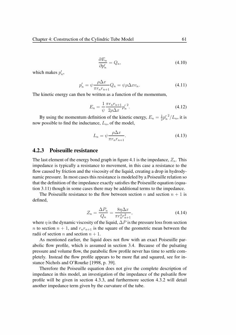
Chapter 4: Construction of the Cylindric Tube Model 61
∂En∂p′n
= Qn, (4.10)
which makes p′n,
p′n = ψρ∆x
πrnrn+1Qn = ψρ∆xvn. (4.11)
The kinetic energy can then be written as a function of the momentum,
En =1
ψ
πrnrn+1
2ρ∆xp′n
2. (4.12)
By using the momentum definition of the kinetic energy, En = 12p′n
2/Ln, it isnow possible to find the inductance, Ln, of the model,
Ln = ψρ∆x
πrnrn+1. (4.13)
4.2.3 Poiseuille resistance
The last element of the energy bond graph in figure 4.1 is the impedance, Zn. Thisimpedance is typically a resistance to movement, in this case a resistance to theflow caused by friction and the viscosity of the liquid, creating a drop in hydrody-namic pressure. In most cases this resistance is modeled by a Poiseuille relation sothat the definition of the impedance exactly satisfies the Poiseuille equation (equa-tion 3.11) though in some cases there may be additional terms to the impedance.
The Poiseuille resistance to the flow between section n and section n + 1 isdefined,
Zn =∆PnQn
=8η∆x
πr2nr2n+1
, (4.14)
where η is the dynamic viscosity of the liquid, ∆P is the pressure loss from sectionn to section n + 1, and rnrn+1 is the square of the geometric mean between theradii of section n and section n+ 1.
As mentioned earlier, the liquid does not flow with an exact Poiseuille par-abolic flow profile, which is assumed in section 3.4. Because of the pulsatingpressure and volume flow, the parabolic flow profile never has time to settle com-pletely. Instead the flow profile appears to be more flat and squared, see for in-stance Nichols and O’Rourke [1998, p. 39].
Therefore the Poiseuille equation does not give the complete description ofimpedance in this model, an investigation of the impedance of the pulsatile flowprofile will be given in section 4.3.3, and furthermore section 4.3.2 will detailanother impedance term given by the curvature of the tube.

62 Mathematical Modeling of Flow Characteristics in the Embryonic Heart
4.2.4 The Bernoulli effect
All elements of the energy bond graph in figure 4.1 are now described, the firstand the last element in the figure are to be considered as boundary conditions forthe model and as such they will change according to the use of the model, forinstance on section 5.2 they are completely absent. The simple explanation of theelements is complete, but there is more to be done in constructing the cylindrictube model.
Notice how the dynamic radius, rn, is included in the expression for all theelements of the model, but at the same time rn is part of the charge variable atthe untransformed capacitance, ∆rn = rn − Rn. It seems that there is a couplingbetween the elements, which should be explored.
Let the total energy of the transmission line be named E, it will be a sum ofpotential and kinetic energies of all the sections of the tube. The derivative of Ewith respect to the charge variable, ∆rn, will yield the potential variable. Thisreveals a relation between charge and potential, which is not directly reflected inthe model,
∂E
∂rn=
∂ (Un + En−1 + En)
∂rn
= 2πFn +1
ψ
π
2ρ∆x
(rn−1p
′n−1
2+ rn+1p
′n2)
= 2πrn∆x
(Pn +
ρ
4ψ
(rn−1
rnv2n−1 +
rn+1
rnv2n
)). (4.15)
Notice that the factor, 2πrn∆x, is the transformation ratio, Tn, from the section4.2.1. It is seen that the potential is not only composed of the pressure, whichwas specified from the start, but also has two extra terms coming from the kineticenergy. Overall expression 4.15 bear a certain likeness to the Bernoulli equation(equation 3.17), with the two extra terms being some sort of kinetic pressure. Thisconnection to the Bernoulli equation will be investigated further below.
Furthermore it is clear that the capacitance and the inductance of the modelare not independent of each other, both are functions of the dynamic radius andthe radius is itself a variable of the section. Thus write the dynamic radius as afunction of the capacitance,
rn =
√
C ′n
Eh
2π∆xRn, (4.16)
which makes it obvious that the inductance can be written as a function of thecapacitance,

Chapter 4: Construction of the Cylindric Tube Model 63
Ln = ψρ∆x
πrnrn+1= ψ
2ρ∆x2
Eτ
√√√√RnRn+1
C ′nC
′n+1
. (4.17)
The inductance depends on the capacitance of the section and the capacitanceof the next section, which makes sense since the capacitance models how muchliquid each section can hold (under the given pressure), and the inductance modelsthe inertia of the total amount of liquid flowing from one section to the next.Mathematically this is not a problem for the model, but physically it is desirableto have all elements described as independent physical constants and let currentand potential be the only variables of the system.
The almost-Bernoulli relation of equation 4.15 and the inter-dependency ofthe elements point to the fact that this model is still incomplete, there are hiddenqualities of the model that need to be explicitly reflected in the energy bond graph.To do this, a new momentum variable is introduced by inserting a transformer infront of the inductance in the energy bond diagram in figure 4.1. Mathemati-cally this corresponds to a transformation of variables by the transformation ratio,√rnrn+1/RnRn+1, which gives the momentum,
pn =
√rnrn+1
RnRn+1p′n =
√rnrn+1
RnRn+1ψρ∆xvn. (4.18)
This yields a new expression for the kinetic energy,
En =1
ψ
πrnrn+1
2ρ∆x
(√RnRn+1
rnrn+1
pn
)2
=1
ψ
πRnRn+1
2ρ∆xp2n, (4.19)
and hence also a new rn-independent expression for the inductance,
Ln =p2n2En
= ψρ∆x
πRnRn+1. (4.20)
In the definition of the new momentum of flow it is interesting to observewhat this means for the potential input to the inductance, this is found by takingthe time-derivative of the momentum,
dpndt
=
√rnrn+1
RnRn+1
dp′ndt
+1
2
p′n√RnRn+1
(√rn+1
rn
drndt
+
√rnrn+1
drn+1
dt
)
=
√rnrn+1
RnRn+1
dp′ndt
+1
2
pn√rnrn+1
(√rn+1
rn
drndt
+
√rnrn+1
drn+1
dt
)
=
√rnrn+1
RnRn+1
dp′ndt
+pn2rn
drndt
+pn
2rn+1
drn+1
dt. (4.21)

64 Mathematical Modeling of Flow Characteristics in the Embryonic Heart
Notice here that the input potential to the inductance comes partially from thetransformed momentum and partially from two other sources. The time-derivativeof the dynamic radius is the current into the capacitance of the system, and so bythe transformation of the momentum it has become clear that the input potentialto the inductance has contributions from the current at the capacitors on eitherside of the inductance. The current is however changed from current to potentialthrough the ratio, pn/2rn on the lower side and pn/2rn+1 on the upper side.
With this restructuring of the transmission line the energy derivative fromequation 4.15 can be redone,
∂E
∂rn= 2πFn +
1
ψ
π
2ρ∆x
(rn−1p
′n−1
2+ rn+1p
′n2)
= 2πFn +1
ψ
π
2ρ∆x
(Rn−1Rn
rnp2n−1 +
RnRn+1
rnp2n
)
= 2πFn +pn−1
2rn
pn−1
Ln−1
+pn2rn
pnLn, (4.22)
which corresponds exactly to the output potential from the capacitance plus twocontributions from the inductances on either side that have been converted throughthe relations pn−1/2rn and pn/2rn. In other words this is the potential given by thederivative of the total energy with respects to the charge variable, ∆rn, it has theunits of force and through the transformation ratio 2π∆xrn the driving pressurefor section n is found,
Pn =1
2π∆xrn
(2πFn +
pn−1
2rn
pn−1
Ln−1+
pn2rn
pnLn
)
=Fn
∆xrn+
1
2π∆xrn
(rn−1
ψπρ∆x
2v2n−1 + rn+1
ψπρ∆x
2v2n
)
=Fn
∆xrn+ ψ
rn−1
2rn
1
2ρv2n−1 + ψ
rn+1
2rn
1
2ρv2n. (4.23)
From this equation it can be seen that the driving pressure consists of the hydro-dynamic pressure, Fn/∆xrn, and a ‘kinetic pressure’ that is consistent with theBernoulli equation except that it is calculated as an average of the inflow and out-flow velocities of a section of the tube and weighted by the ratio of the radius tothe radii of the adjacent sections.

Chapter 4: Construction of the Cylindric Tube Model 65
4.3 Additional effects
With the Bernoulli coupling the cylindric tube model has come so far that it isoperational, as specified in the descriptions above the energy bond graph has beenmodified from that of the transmission line in figure 4.1 through use of variabletransformations to the energy bond graph in figure 4.2.
In the figure it is still possible to see the basic setup consisting of a capacitance,inductance and a resistor, but in addition the triangle symbols represent the trans-formation of variables mentioned in equation 4.4 and 4.18 and the fish-shapedsymbols represent another set of variable transformations presented in equation4.22, though these gyrators as they are called have the special effect that theytransform current to potential and vice versa.
√rnr
n+1
RnRn+12π∆xrn 2π∆xrn+1
Qn QnQn−1 Qn+1Pn Pn+1
Zn
pn2rn
pn2r
n+1
Cn Ln Cn+1
2πFn
rn2πFn+1
rn+1
rn rn+1pn
Figure 4.2: The energy bond graph of the expansion to the transmission line. Thefigure only shows one and a half section in the transmission line, but notice thatthe elements of the section have been switched around compared to figure 4.1 sothat the potential storage comes before the kinetic storage.
The definitions of elastic capacitance, inertia of mass, Poiseuille resistanceand the Bernoulli effect constitute the core effects of the model, but the model isstill in the rough. The next step is to improve the model with additional effectsthat increase the model’s applicability in relation to the liquid flow in an elastictube: the longitudinal tensions of the tube counteracting lengthwise discrepanciesbetween different radii of neighboring sections, the resistance induced by tubecurvature on the pressure and flow, and the Womersley theory for pulsatile pres-sure and flow. The three effects will be presented one by one and explained howthey are implemented in the model.

66 Mathematical Modeling of Flow Characteristics in the Embryonic Heart
4.3.1 Longitudinal shear tensions
One adjustment to the model comes from the logical fact that when the radius ofone section of the tube is increased the wall of the section will pull the walls ofthe neighboring sections. The sections are not independent and thus the radiusincrease is not only a function of the liquid volume of the section itself but also afunction of the radii of the neighboring sections. This interaction of the radii ofthe various sections is governed by the elastic forces tangential to the tube, whichare described as shear tensions of the tube wall.
The shear tensions of the tube wall describe the wall’s response to a skewdeformation when one section’s surface area becomes larger than its neighbor’s,but as all skew deformations can be transformed into right angle deformations theshear tensions will also describe the wall’s response to a longitudinal strain of itslength. As such this addition to the model is also supposed to reflect how theperiodic pressure waves produce longitudinal stresses in the tube, even though thelength of the tube is fixed in the model. Therefore this addition to the model willhave a more ad hoc character compared to the previous model elements.
When the radii of two neighboring sections differ from their resting valuesby unequal increments a force will act between them trying to pull the differencetowards zero. This force, which has both tangential and longitudinal compos-ites, is proportional to the difference in radial change between the sections andit is given by the shear modulus, G, which for isotropic materials is one thirdof Young’s modulus (since the shear modulus models a one dimensional responsewhile Young’s modulus has three dimensions). The calculation of the elastic force,Fsn, is analogue to the elastic force for the radius expansions in section 4.2.1,
Fsn =Gh
√RnRn+1
∆x(∆rn+1 −∆rn) , (4.24)
where√RnRn+1 is the geometric mean between the resting radii of the two neigh-
boring sections. This force is integrated over the circumference (multiply with 2π)and integrated over the difference from ∆rn to ∆rn+1,
Usn =∫ ∆rn+1
∆rn2πGh
√RnRn+1
∆x(∆rn+1 −∆r′) d∆r′
=πGh
√RnRn+1
∆x(∆rn+1 −∆rn)
2 . (4.25)

Chapter 4: Construction of the Cylindric Tube Model 67
Insert the energy from equation 4.25 into the formula for the potential energyof a capacitor, Usn = 1
2(∆rn+1 −∆rn)
2 /Csn, to find the capacitance,
Csn =∆x
2πGh√RnRn+1
. (4.26)
The capacitance, Csn, models the elastic attraction between two neighboringsections, for a soft tube the capacitance is high and the radii of neighboring sec-tions are allowed to diverge more easily.
On the other hand diverging radii of neighboring sections will also cause fric-tion inside the tube wall. Friction equals loss of energy thus an resistance is neededto model the shear tensions of the wall, with impedance proportional to the differ-ence in radial change between the two sections.
In the model the impedance, Zsn, is an ad hoc determined constant, whichis given from the desire that oscillations with frequencies above 100 Hz shouldbe damped. The impedance is determined through the fact that the period of anoscillation in an RC-circuit is given by T = ZsnCsn, which by insertion of thedesired period, T = 0.01 seconds, yields the impedance, Zsn = T/Csn.
4.3.2 Curvature of the tube
Another addition to the model is the resistance given by the curvature of the tube.When liquid flows through a bent tube a lot of interesting things happen and it isclear that the standard Poiseuille equation will not fully describe the flow, even ifit is still laminar, in fact it has been demonstrated that the location of maximumaxial velocity shifts towards the outer wall of a curved tube [Berger et al., 1983].
Even more interesting is the establishment of so called secondary flow whereliquid performs a rotating motion at right angles to the axis of the tube. Thissecondary flow is a consequence of the centrifugal pressure gradient in the benttube acting together with the friction of the tube walls, it is generally superimposedupon the main flow and is present in both laminar and turbulent flows [Crane Co.,1982].
Generally the flow through a bent tube depends on only two characteristicsof the bend, the angle of the bend and its curvature. These are compared to theReynolds number of the flow to establish if the bend is ’smooth’ in relation to theflow [Crane Co., 1982]. If the bend is too sharp eddies will form at the inner wall,which will impact flow before and mainly after the bend and increase energy lossin the bend. For higher Reynolds numbers the turbulent flow will cover more areaof the bent tube.
Despite of these phenomena the main effect of a bent tube on the liquid flow isa loss of energy, which can be seen as a pressure drop from the frontal to distal endof the bend. In general a pressure drop in the tube is given by Darcy’s equation,

68 Mathematical Modeling of Flow Characteristics in the Embryonic Heart
∆P = f∆x
2R
ρv2
2, (4.27)
where ∆x is the length of tube andR is its radius, ρ is the density of the liquid andv is the typical velocity of the liquid through the tube. The typical velocity of theliquid is unspecified in Darcy’s equation to the extent that it is the same velocityas used in the definition of the Reynolds number and generally it is taken to be themean velocity, v = Q/πR2.
The quantity f in equation 4.27 is the friction factor, which details the energyloss of the flow through that particular length of tube. For a straight tube thefriction factor is dependent on the Reynolds number, for laminar flow (Re <1000) the friction factor is a function of the Reynolds number alone, f = 32
Re=
32ηρvR
,
∆P =32η
ρvR
∆x
2R
ρv2
2=
8η∆xv
R2=
8η∆x
πR4Q, (4.28)
thus Darcy’s equation becomes the Poiseuille equation.For completely turbulent flow (Re > 2000) the friction factor is a function of
the Reynolds number as well as the roughness of the tube wall. There is no simpleequation that governs friction factors in this regime but the Blasius law seems tobe a good approximation for the lower bounds of turbulent friction factors in acompletely smooth tube [Keller, 1978, p. 49],
fturbulent =0.3164√2Re
. (4.29)
ForRe ∈ [1000; 2000] the flow can be either laminar or turbulent, and thus thefriction factor may vary between the values of the friction factors of laminar andturbulent flow as the lower and upper bound [Crane Co., 1982].
For any sort of circumstance imposed on the tube, such as bends, contractions,valves and branches, there is a corresponding friction factor, which will give thepressure loss for that instance. Collectively these pressure losses are known asminor losses. For each instance the friction factor will be an empirical numberthat has to be found experimentally but common engineering practice dictates thatit will be sufficient to extrapolate from known values of likened effects [Crane Co.,1982].
The clever thing about writing the pressure loss with Darcy’s equation is thatfriction coefficients are cumulative by definition, and thus the pressure loss asso-ciated with the flow through a curved tube will be defined,
∆P = (fL + fB)∆x
2R
ρv2
2, (4.30)
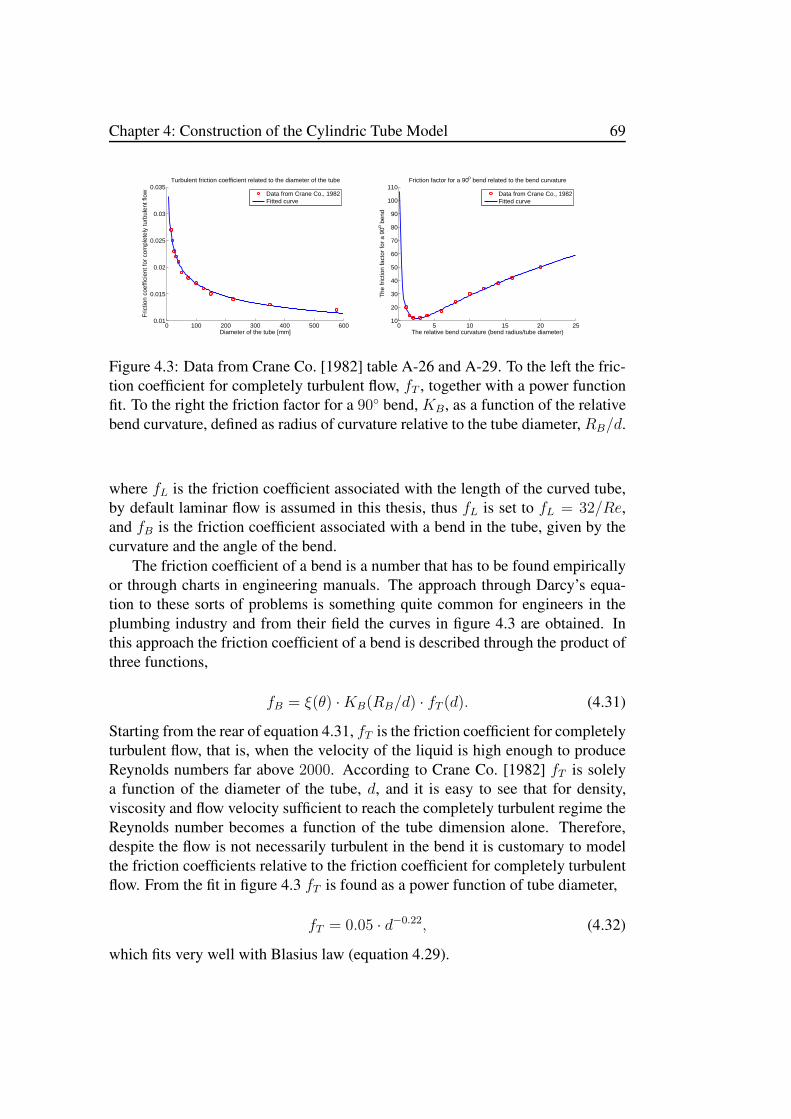
Chapter 4: Construction of the Cylindric Tube Model 69
0 100 200 300 400 500 6000.01
0.015
0.02
0.025
0.03
0.035Turbulent friction coefficient related to the diameter of the tube
Diameter of the tube [mm]
Fric
tion
coef
ficie
nt fo
r co
mpl
etel
y tu
rbul
ent f
low
Data from Crane Co., 1982Fitted curve
0 5 10 15 20 2510
20
30
40
50
60
70
80
90
100
110Friction factor for a 90o bend related to the bend curvature
The relative bend curvature (bend radius/tube diameter)
The
fric
tion
fact
or fo
r a
90o b
end
Data from Crane Co., 1982Fitted curve
Figure 4.3: Data from Crane Co. [1982] table A-26 and A-29. To the left the fric-tion coefficient for completely turbulent flow, fT , together with a power functionfit. To the right the friction factor for a 90 bend, KB, as a function of the relativebend curvature, defined as radius of curvature relative to the tube diameter, RB/d.
where fL is the friction coefficient associated with the length of the curved tube,by default laminar flow is assumed in this thesis, thus fL is set to fL = 32/Re,and fB is the friction coefficient associated with a bend in the tube, given by thecurvature and the angle of the bend.
The friction coefficient of a bend is a number that has to be found empiricallyor through charts in engineering manuals. The approach through Darcy’s equa-tion to these sorts of problems is something quite common for engineers in theplumbing industry and from their field the curves in figure 4.3 are obtained. Inthis approach the friction coefficient of a bend is described through the product ofthree functions,
fB = ξ(θ) ·KB(RB/d) · fT (d). (4.31)
Starting from the rear of equation 4.31, fT is the friction coefficient for completelyturbulent flow, that is, when the velocity of the liquid is high enough to produceReynolds numbers far above 2000. According to Crane Co. [1982] fT is solelya function of the diameter of the tube, d, and it is easy to see that for density,viscosity and flow velocity sufficient to reach the completely turbulent regime theReynolds number becomes a function of the tube dimension alone. Therefore,despite the flow is not necessarily turbulent in the bend it is customary to modelthe friction coefficients relative to the friction coefficient for completely turbulentflow. From the fit in figure 4.3 fT is found as a power function of tube diameter,
fT = 0.05 · d−0.22, (4.32)
which fits very well with Blasius law (equation 4.29).

70 Mathematical Modeling of Flow Characteristics in the Embryonic Heart
KB is the friction factor that is multiplied to fT for a tube bend of exactly90. Plumbers work mostly with right angle fittings and thus the data comes frommeasurement of pressure loss through those. Different fittings can have differentcurvature, and thus KB is a function of the relative curvature defined as the curva-ture radius for the center-line of the tube bend, RB , relative to the tube diameter,d. Figure 4.3 shows data from Crane Co. [1982], the data is fitted to the function,
KB(RB/d) = 9.07 (ln(RB/d))2 − 16.93 ln(RB/d) + 19.64. (4.33)
The final function of equation 4.31, ξ(θ), is the angular factor for bend anglesdifferent from 90. The angle of the bend, θ, is defined as the angle between thedirections of the tube before and after the bend, thus a straight tube would haveθ = 0. Keller [1978, p. 49] defines the function,
ξ(θ) = 0.042 · θ0.69. (4.34)
In the end the friction factor, f = fL + fB = 32/Re + ξKBfT , lets Darcy’sequation be converted to the Poiseuille equation plus an extra term,
∆P =8η∆x
πR4Q + ξKBfT
∆x
2R
ρv2
2
=8η∆x
πR4Q +
(0.018
(lnRB
d
)2
− 0.034 lnRB
d+ 0.039
)θ0.69
d0.22∆x
2R
ρv2
2
=8η∆x
πR4Q +
(3.9
(lnRB
d
)2
− 7.3 lnRB
d+ 8.4
)10−3ρ∆xθ
0.69
π2R5.22Q2.
(4.35)
As can be seen in equation 4.35 the last term is quadratic with respect to the flow.Thus it do not directly fit into the linear approach of the energy bond formalism.
With the curvature of the tube two distinct frictional effects are defined in therelation between flow and pressure, and equation 4.35 demonstrates quite simplythat they will be serially coupled in the energy bond graph. The first frictionaleffect is the Poiseuille resistance, which has already been described, the other isthe friction of the bend. In the energy bond graph the friction will be representedby an impedance symbol, ZB, that links a pressure loss to the flow rate,
ZBn =∆PnQn
= ξKBfTρ∆xQn
4π2√rnrn+15 . (4.36)
In terms of the energy bond formalism, which relies on linear response theory, thisequation is erroneous; the volume flow is not allowed to be part of the response

Chapter 4: Construction of the Cylindric Tube Model 71
function while it is input to the function. Instead notice that this equation hasresemblance to the momentum of the flow defined in equation 4.18,
pn =
√rnrn+1
RnRn+1
p′n = ψ
√rnrn+1
RnRn+1
ρ∆x
πrnrn+1
Qn, (4.37)
and thus the impedance of the bend can be written using the momentum ratherthan the flow (where the numerical value of the momentum is used because theimpedance should cause a loss of energy independent of the direction of flow),
ZBn =∆PnQn
=ξKBfTψ
√RnRn+1
4πr2nr2n+1
|pn|. (4.38)
Equation 4.38 defines the additional friction of the bend as a relation betweenpressure loss to volume flow. Interestingly this impedance is proportional to thenumerical value of the momentum of the flow, thus it grows when flow is acceler-ated, which is very interesting in relation to pulsating flow and pressure.
4.3.3 Womersley theory
The final addition to the model it the inclusion of Womersley theory to express theinfluence by the velocity profile on the nature of the flow in a tube.
With regards to the behavior of regular pulsating blood flow it has been arguedby many physicians and researchers that the Poiseuille equation is not the bestdescription for the interrelation between volume flow and pressure gradient whenboth are pulsating with time, see for instance the list of restrictions in section 3.4.Such was also the view of mathematician John R. Womersley who in the 1950’iesstruck a productive cooperation with the established doctor of physiology DonaldA. McDonald, and together they became a very important chapter in the historyof blood flow research [Nichols and O’Rourke, 2008].
Womersley’s approach to the problem of pulsatile blood flow was to analyzethe Navier-Stokes equation under assumptions applicable to blood in the arteries.
Under the simple assumption that the pressure gradient, ∇P , and the flowvelocity field, v, are both unchanged with time the Navier-Stokes equation ofincompressible liquid,
ρ
(∂v
∂t+ v · ∇v
)= −∇P + η∇2
v + f , (4.39)
with ρ, η and f being liquid density, dynamic viscosity and external forces onthe infinitesimal liquid volume respectively, under the restrictions of a cylindricaltube is written,

72 Mathematical Modeling of Flow Characteristics in the Embryonic Heart
d2v
dr2+
1
r
dv
dr+
1
η
∆P
∆x= 0, (4.40)
where ∇P = ∆P/∆x is the pressure gradient found by subtracting pressuresat two different points on the longitudinal axis of the tube and dividing by thedistance between them, ∆x.
Notice that pressure may change with the longitudinal axis of the tube, thepressure gradient is a constant, whereas the flow velocity may change with theradial position in the tube but not with the longitudinal coordinate. The solution tothis equation gives the flow velocity, v(r) = ∆P
4η∆x(R2 − r2), whereR is the radius
of the tube, and with volume flow defined as the integral, Q = 2π∫R0 v(r)rdr, the
Poiseuille equation is achieved,
Q =πR4
8η∆x∆P. (4.41)
In contrast Womersley allowed both flow velocity field and pressure gradientto vary with time, though pressure is radially constant and the velocity field isunchanged with the longitudinal coordinate, which yields the following equation,
∂2v
∂r2+
1
r
∂v
∂r− ρ
η
∂v
∂t+
∆P (t)
η∆x= 0. (4.42)
Assume the time variant pressure difference has a constant and a varying term,∆P (t) = ∆P0 + ∆P (t), with ∆P (0) = 0 and ∆P (T ) = ∆P (0) for someT > 0. Due to linearity a simple particular solution to the constant term willbe the Poiseuille equation, v0(r) = ∆P0
4η∆x(R2 − r2). The complete solution to
equation 4.42 will be given on the form,
v(r, t) =∞∑
n=1
(AnJ0
(r√−kn
)+BnY0
(r√−kn
))ekn
ηρt
+
(∫ t
0
∆P (τ)
ρ∆xdτ
)+
∆P0
4η∆x
(R2 − r2
), (4.43)
where J0 and Y0 are Bessel functions of the first and second kinds of order zero,however the limit, limz→0 Y0(z) = −∞, forces Bn = 0 for a real solution. Fur-thermore the boundary condition v(R, t) = 0 forces An = −an
ρ∆xJ0(R√−kn)
, where
an is a new arbitrary constant that will be determined later, so that,
v(r, t) =∞∑
n=1
−anρ∆x
J0(r√−kn
)
J0(R√−kn
)eknηρt +
∫ t
0
∆P (τ)
ρ∆xdτ +
∆P0
4η∆x
(R2 − r2
).
(4.44)
Chapter 4: Construction of the Cylindric Tube Model 73
The equation is rewritten with the definition of volume flow,
Q(t) = 2π∫ R
0
∞∑
n=1
−anρ∆x
J0(r√−kn
)
J0(R√−kn
)eknη
ρtrdr
+2π∫ R
0r∫ t
0
∆P (τ)
ρ∆xdτdr + 2π
∫ R
0
∆P0
4η∆x
(R2 − r2
)rdr
=∞∑
n=1
−an2πRρ∆x
√−kn
J1(R√−kn
)
J0(R√−kn
)eknη
ρt +
πR2
ρ∆x
∫ t
0∆P (τ)dτ +
πR4
8η∆x∆P0.
(4.45)
The obvious case suggests itself that volume flow and pressure gradient in-side the blood vessels can be described with a Fourier series, which was exactlyone of the questions in the research by Womersley and McDonald [Nichols andO’Rourke, 2008]. Assume that the pressure difference is a periodic function, withangular frequency, ω, described with the Fourier series,
∆P (t) =∞∑
n=1
∆Pneinωt. (4.46)
The no-slip boundary condition, v(R, t) = 0, will then enforce an = ∆Pn
inωand
kn = inω ρη. Thus the oscillating volume flow becomes
Q(t) =∞∑
n=1
−∆Pn2πR
inωρ∆x√−inω ρ
η
J1
(R√−inω ρ
η
)
J0
(R√−inω ρ
η
)einωt
+∞∑
n=1
πR2
inωρ∆x∆Pne
inωt +πR4
8η∆x∆P0
=∞∑
n=1
πR2
ρ∆x
∆Pninω
1−
2
R√−inω ρ
η
J1
(R√−inω ρ
η
)
J0
(R√−inω ρ
η
)
e
inωt +πR4
8η∆x∆P0
=πR4
η∆x
[∞∑
n=1
−∆Pn
R2√−inω ρ
η
2
1−
2
R√−inω ρ
η
J1
(R√−inω ρ
η
)
J0
(R√−inω ρ
η
)
e
inωt
+∆P0
8
]. (4.47)

74 Mathematical Modeling of Flow Characteristics in the Embryonic Heart
From equation 4.47 it is clear that the relation between volume flow and pres-sure gradient is much more complex than the Poiseuille equation, specifically therelation depends on the angular frequency. To analyze this relation Womersley de-fined the non-dimensional parameter popularly known as the Womersley number[Womersley, 1955b],
α = R
√ωρ
η. (4.48)
With the Womersley number examine the oscillating part of the volume flow, thatis, the constant term Q0 = πR4
8η∆x∆P0 is disregarded for the moment. Specifically
of interest is the function inside the brackets in equation 4.47,
f(α, n) = 1− 2
α√−in
J1(α√−in
)
J0(α√−in
) , (4.49)
f(α, n) is a complex function with Ref(α, n) ∈ [0, 1] and Imf(α, n) ≥ 0 andwith limn→∞ f(α, n) = 1+0i. Womersley recognized that the behavior of f(α, n)could generally be divided into three cases:
For α < 1 and for n small f(α, n) ≈ 0 + 0i. In this case the lowest line ofequation 4.47 is of interest; recognize that the function f(α,n)
inα2 ≈ 18+ 0i for small
values of n and goes to zero for higher values of n. As could be expected for lowvalues of α equation 4.47 approaches the Poiseuille equation, this let Womersleyconclude that for small frequencies the oscillating flow is dominated by friction,through one period the flow will have time to establish a parabolic flow profile,which is sufficiently described with the Poiseuille equation [Womersley, 1955b].
For α > 10 the function f(α, n) ≈ 1 + 0i for all values of n. In this case themiddle line of equation 4.47 is of interest; recognize that with f(α, n) basically aconstant, the flow is given by a relation to the integral of the pressure difference,which by definition is the momentum of the flow, p(t). Therefore with high valuesof α the oscillating volume flow is dominated by inertia and in simple terms it canbe approximated with the equation,
Q(t) =πR2
ρ∆xp(t). (4.50)
In the intermediate regime, 1 < α < 10, the oscillating volume flow is nei-ther completely dominated by friction or inertia, and the function f(α, n) has asignificant imaginary part. Unfortunately for Womersley blood flow in the largermammalian and human arteries tend to fall inside this range [Womersley, 1955a].
To give a tangible solution for the volume flow approximate f(α, n) with n tothe first order,

Chapter 4: Construction of the Cylindric Tube Model 75
0 5 10 15−0.1
0
0.1
0.2
0.3
0.4
0.5
0.6
0.7
0.8
0.9
Function of the Womersley number
α−value
func
tion−
valu
e
Re(f(α,1)/iα2)
Re(f(α,1))
Im(f(α,1))
Im(f(α,1)/iα2)
Figure 4.4: The function f(α, n) = 1− 2α√−in
J1(α√−in)
J0(α√−in)
for n = 1 as the defining
function for the time variant pressure and volume flow.
f(α, 1) = 1− 2
α√−i
J1(α√−i)
J0(α√−i) , (4.51)
as figure 4.4 demonstrates this function is almost zero for α < 1 and nearly con-stant and real for α > 10. For higher orders of n the transition from zero toone will only be more steep. With this function define an approximate solutionto the time variant volume flow given by equation 4.45 through a combination offrictional and inertial effects (still without the constant term),
Q(t) ≈ πR2
ρ∆x
1− 2
α√−i
J1(α√−i)
J0(α√−i)
p(t)
≈ πR4
η∆x
1
iα2
1− 2
α√−i
J1(α√−i)
J0(α√−i)
∆P (t). (4.52)
Depending on the scale of α either of the two lines of equation 4.52 may be chosenas the approximation to the time variant volume flow.
Furthermore, rearranging equation 4.52 yields the relation,
η∆x
πR4(8 + Ψ(α))Q(t) =
η
ρ
1
R2iα2p(t), (4.53)

76 Mathematical Modeling of Flow Characteristics in the Embryonic Heart
where
Ψ(α) =iα2
1− 2α√−i
J1(α√−i)
J0(α√−i)
− 8, (4.54)
and where α2 = R2ω ρη
so that the right hand side can be replaced by the timevariant pressure difference. In this way equation 4.53 shows that the pressuredifference is made of two terms, one Poiseuille term defined by the low frequencylimit of the function 1
iα2 f(α, 1) and one other term defined by the function Ψ(α).
Name the Poiseuille term ∆Pp(t) and the other term ∆Pψ(t),
η∆x
πR4(8 + Ψ(α))Q(t) = ∆Pp(t) +
η
ρ
1
R2iα2pψ(t), (4.55)
where pψ(t) is the momentum referring to ∆Pψ(t). The Poiseuille term cancelsout of the relation by use of Poiseuille’s equation, which leaves the expression,
η∆x
πR4Ψ(α)Q(t) =
η
ρ
1
R2iα2pψ(t)
ρ∆x
πR2ψ(α)Q(t) = pψ(t). (4.56)
The function ψ(α) is defined,
ψ(α) =1
1− 2α√−i
J1(α√−i)
J0(α√−i)
− 8
iα2, (4.57)
and gives the magnitude of the extra term in equation 4.55 for any value of α. Asfigure 4.5 demonstrates ψ(α) is a complex function with real values in the rangefrom 1 for high values of α to 4/3 for low values of α and with imaginary valuesdifferent from zero only in the transition, notably for α-values from 1 to 10.
For higher orders of n in equation 4.49 a similar result is obtained, assumingthat cross-terms are negligible, for each n a function like ψ(α) can be defined,which will have real values in the range from 1 to 4/3 and imaginary values dif-ferent from zero only in the transition. The transition itself will only be sharperfor higher values of n.
Thus it is assumed that the function ψ(α) for n = 1 is a sufficient approxima-tion and that the complete description of the volume flow to pressure gradient canbe described with a Poiseuille term of the pressure difference plus a momentumterm given by the function ψ(α),
Q(t) =πR4
8η∆x∆P (t) +
1
ψ(α)
πR2
ρ∆xpψ(t). (4.58)

Chapter 4: Construction of the Cylindric Tube Model 77
0 10 20 30 40 50−0.2
0
0.2
0.4
0.6
0.8
1
1.2
1.4ψ−function of the Womersley number
α−value
ψ(α
)
Re(ψ(α))
Im(ψ(α))
Figure 4.5: The function ψ(α) = 1
1− 2α√
−i
J1(α√
−i)J0(α
√−i)
− 8iα2 as the defining function for
the extra momentum contribution to the time variant pressure and volume flow.
Equation 4.58 reveals how the inertia of the liquid depends on the flow profile,which was discussed in section 3.8, and demonstrates how the inductance definedin section 4.2.2 is modified with the function ψ(α) defined in equation 4.57.
4.4 The use of the model
The Womersley factor concludes the last addition to the model and reveals howthe factor ψ introduced in section 4.2.2 is given by at function found by the solu-tion of the Navier-Stokes equations under the assumptions of a pulsatile flow andpressure.
With the additions of shear tensions, curvature resistance and the Womersleyfactor to the model the energy bond graph will be changed as shown in figure 4.6,both the capacitance and impedance of the shear tensions are visible at the top ofthe model, and the resistance from curvature is visible below, while the Womersleyfactor is not directly visible in the model as it is a factor in the calculation of theinductance, Ln.
It is apparent that this model is non-linear and that none of the elements inthe model are directly constant compared to the pressure and volume flow, thedynamic radius seems to play an important role in their relations as well as themomentum of flow. Since the value of some elements depend on parameters de-fined as output from other elements in the energy bond graph it is not possible

78 Mathematical Modeling of Flow Characteristics in the Embryonic Heart
√rnr
n+1
RnRn+1
2π∆xrn 2π∆xrn+1
Qn QnQn−1 Qn+1Pn Pn+1
Zn ZBn
pn2rn
pn2r
n+1
Cn Cn+1
Ln
2πFn 2πFn+1
rn rn+1
rn rn+1
pn
rn rn+1
Zsn
Csn
Figure 4.6: The final appearance of the energy bond graph for the cylindricalmodel. The standard layout of the transmission line is still an important factor inthe model, but it has been changed to better describe liquid flow in an elastic tube.The capacitance and resistance, Csn and Zsn, are secondary effects to reduce theflexibility of the arterial wall, while the resistance ZBn is included to model theresistance induced by the curvature of the tube.
to make a simple simulation of the model of the kind normally understood fromenergy bond graphs or electrical networks. Instead an approximative simulationprocedure must be constructed by a Runge-Kutta iteration of the variables of themodel.
For this iterative solution procedure the rates of change of the radius and themomentum of the flow are used for a progressive numerical Runge-Kutta solutionof their respective differential equations to find their state variables as functionsof time, and from those the variables of pressure and flow are calculated.
The time-dependent values of pressure and volume flow are used as dummyvariables in the calculations of the rates of change of radial change and momentumof the flow, it is useful to identify those before calculating the rates of change. Inthe energy bond graph in figure 4.6 the volume flow, Qn, is given by the back-transformed output from the inductance, Ln,

Chapter 4: Construction of the Cylindric Tube Model 79
Qn =pnLn
√rnrn+1
RnRn+1
. (4.59)
Likewise the pressure is given by the output from the capacitance, Cn, but alsofrom the adjacent capacitances, Csn, and their related resistances, Zsn. In additionthe Bernoulli effect adds contributions from the adjoined inductances, Ln−1 andLn, through the gyration ratios, pn−1
2rnand pn
2rn. All this is transformed back by the
transformation ratio, 2π∆xrn. This corresponds to the combined potential in thefirst O-junction of the network,
Pn =1
2π∆xrn
(rn −Rn
Cn+rn − rn−1
Csn−1
+ Zsn−1
(drndt
− drn−1
dt
)
−rn+1 − rnCsn
− Zsn
(drn+1
dt− drn
dt
)+pn−1
2rn
pn−1
Ln−1+
pn2rn
pnLn
).
(4.60)
The rate of change for the radius of a section of the tube is the current variablein the left vertical branch of the energy bond graph in figure 4.6, which constitutethe input to the capacitance, Cn. This current variable is given by the transforma-tion, 2π∆xrn, of the current variable below the first transformer in the network,and this current is given as the difference between inflow and outflow to the o-junction in the network. This corresponds to the fact that the change in radius isfound by the change in volume given by the difference in volume flow in relationto the surface area of the section,
drndt
=Qn−1 −Qn
2π∆xrn=
1
2π∆xrn
(pn−1
Ln−1
√rn−1rnRn−1Rn
− pnLn
√rnrn+1
RnRn+1
). (4.61)
In the same way the rate of change for the momentum of the flow is the input tothe inductance, Ln, this is a potential variable and thus it is found by adding all theincoming potential contributions to the X-junction in front of the inductance. Theincoming potential is firstly given by the rate of change of radii of the borderingsections that is changed into a potential through the gyrators, and secondly it isgiven by the transformation of the pressure difference given by the difference inpressure between two neighboring sections minus the loss from the Poiseuilleresistance and the resistance due to curvature. Combined, the rate of change ofthe momentum is calculated from the transformation of the pressure differencebetween the the two sections with two contributions from the Bernoulli effect,

80 Mathematical Modeling of Flow Characteristics in the Embryonic Heart
dpndt
=
√rnrn+1
RnRn+1
(P ′n − P ′
n+1 −(
8η∆x
πr2nr2n+1
+ξKBfTψ(α)
√RnRn+1
4πr2nr2n+1
|pn|)Qn
)
+pn2rn
drndt
+pn
2rn+1
drn+1
dt
=
√rnrn+1
RnRn+1
[1
2π∆xrn
(rn −Rn
Cn+rn − rn−1
Csn−1+ Zsn−1
(drndt
− drn−1
dt
)
−rn+1 − rnCsn
− Zsn
(drn+1
dt− drn
dt
)+pn−1
2rn
pn−1
Ln−1+
pn2rn
pnLn
)
− 1
2π∆xrn+1
(rn+1 − Rn+1
Cn+1
+rn+1 − rnCsn
+ Zsn
(drn+1
dt− drn
dt
)
−rn+2 − rn+1
Csn+1− Zsn+1
(drn+2
dt− drn+1
dt
)+
pn2rn+1
pnLn
+pn+1
2rn+1
pn+1
Ln+1
)
− 8η∆x
πr2nr2n+1
√rnrn+1
RnRn+1
pnLn
− ξKBfTψ(α)
√RnRn+1
4πr2nr2n+1
|pn|√rnrn+1
RnRn+1
pnLn
]
+pn2rn
drndt
+pn
2rn+1
drn+1
dt. (4.62)
The rates of change of dynamic radius and momentum of flow are the funda-mental equations of the model. If N is the number of sections in the model therates of change will constitute a system of 2N non-linear differential equations,iterated trough a Runge-Kutta algorithm they yield the time-variant functions ofradius and momentum for all sections of the model, which subsequently can beused to find the time dependent functions of flow and pressure for all sections ofthe model. This will be the solution to the model.
4.5 The continuous limit
An interesting feature of the cylindric tube model worth examination is how themodel behaves when the equations go to the continuous limit by letting ∆x ap-proach zero. In other words, will the equations of the model approach the con-tinuous equations for liquid transport when the model goes from a finite elementmodel to a continuous model. This section is devoted to this question.
Consider the rates of change for a section of the tube, insert the expressions forLn, Cn, Csn and Zsn to have the equations described with only radius, momentumand material constants,

Chapter 4: Construction of the Cylindric Tube Model 81
drndt
=1
2π∆xrn
(πRn−1Rnpn−1
ψ(α)ρ∆x
√rn−1rnRn−1Rn
− πRnRn+1pnψ(α)ρ∆x
√rnrn+1
RnRn+1
),
(4.63)
dpndt
=
√rnrn+1
RnRn+1
[1
2π∆xrn
(2π∆xEh
rn − Rn
Rn
+2πGh√RnRn−1
(rn − Rn)− (rn−1 − Rn−1)
∆x
+0.01 · 2πGh√RnRn−1
∆x
(drndt
− drn−1
dt
)
−2πGh√RnRn+1
(rn+1 − Rn+1)− (rn − Rn)
∆x
−0.01 · 2πGh√RnRn01
∆x
(drn+1
dt− drn
dt
)
+πRnRn−1p
2n−1
2rnψ(α)ρ∆x+
πRnRn+1p2n
2rnψ(α)ρ∆x
)
− 1
2π∆xrn+1
(2π∆xEh
rn+1 − Rn+1
Rn+1
+2πGh√RnRn+1
(rn+1 −Rn+1)− (rn − Rn)
∆x
+0.01 · 2πGh√RnRn+1
∆x
(drn+1
dt− drn
dt
)
−2πGh√Rn+1Rn+1
(rn+2 − Rn+1)− (rn+1 − Rn+1)
∆x
−0.01 · 2πGh√Rn+1Rn+2
∆x
(drn+2
dt− drn+1
dt
)
+πRnRn+1p
2n
2rn+1ψ(α)ρ∆x+πRn+1Rn+2p
2n+1
2rn+1ψ(α)ρ∆x
)
− 8η∆x
πr2nr2n+1
πRnRn+1pnψ(α)ρ∆x
√rnrn+1
RnRn+1
− ξKBfTψ(α)2ρ∆x
√RnRn+1
4πr2nr2n+1
√rnrn+1
RnRn+1πRnRn+1p
2n
]
+pn2rn
drndt
+pn
2rn+1
drn+1
dt, (4.64)
but notice that pn is also dependent on ∆x with the relation
82 Mathematical Modeling of Flow Characteristics in the Embryonic Heart
pn =
√rnrn+1
RnRn+1ψ(α)ρ∆xvn. (4.65)
To find the continuous limit for the equations use the variables rn and vn,which will be defined as functions of space and time, r(x, t) and v(x, t). Let thearterial section n be described by the position x0, thus the equation for the rate ofchange of r(x0, t) becomes
∂r(x0, t)
∂t=
1
2π∆xr(x0, t)
(πR(x0 −∆x)R(x0)
ψ(α)ρ∆x
√√√√r(x0 −∆x, t)r(x0, t)
R(x0 −∆x)R(x0)
·√√√√r(x0 −∆x, t)r(x0, t)
R(x0 −∆x)R(x0)ψ(α)ρ∆xv(x0 −∆x, t)
−πR(x0)R(x0 +∆x)
ψ(α)ρ∆x
√√√√r(x0, t)r(x0 +∆x, t)
R(x0)R(x0 +∆x)
·√√√√r(x0, t)r(x0 +∆x, t)
R(x0)R(x0 +∆x)ψ(α)ρ∆xv(x0, t)
)
=1
2∆x(r(x0 −∆x, t)v(x0 −∆x, t)− r(x0 +∆x, t)v(x0, t))
=1
2∆x
(r(x0 −∆x, t)v(x0 −∆x, t)
−r(x0 +∆x, t)
(v(x0 +∆x, t)−∆x
∂v(x0, t)
∂x
)), (4.66)
where the last step in the equation comes from a first-order Taylor expansion ofv(x0, t). Next, let ∆x approach zero
∂r(x0, t)
∂t= −1
2lim
∆x→0
r(x0, t)v(x0, t)− r(x0 −∆x, t)v(x0 −∆x, t)
∆x
−1
2lim
∆x→0
r(x0 +∆x, t)v(x0 +∆x, t)− r(x0, t)v(x0, t)
∆x
+1
2r(x0, t)
∂v(x0, t)
∂x
= − ∂
∂x(r(x0, t)v(x0, t)) +
1
2r(x0, t)
∂v(x0, t)
∂x
= −v(x0, t)∂r(x0, t)
∂x− 1
2r(x0, t)
∂v(x0, t)
∂x. (4.67)

Chapter 4: Construction of the Cylindric Tube Model 83
Though it may be hard to see, this corresponds exactly to a one-dimensionalcontinuity equation for volume in the tube, ∂V
∂t= − ∂
∂x(V · v). The volume can
be written as V = πr2s, where s is an infinitesimal length of the tube, put thisvolume directly into the continuity equation and observe that the result will beequation 4.67,
∂
∂t
(πsr2(x, t)
)= − ∂
∂x
(πsr2(x, t)v(x, t)
)⇒
2r(x, t)∂r
∂t= −2r(x, t)v(x, t)
∂r
∂x− r2(x, t)
∂v
∂x⇒
∂r
∂t= −v(x, t)∂r
∂x− 1
2r(x, t)
∂v
∂x. (4.68)
For the rate of change of the momentum something similar can be done,though it will not be pretty. Start with equation 4.64 and insert the definitionof the momentum of flow with respect to the mean velocity (equation 4.65),
ψ(α)ρ∆x√RnRn+1
d
dt(√rnrn+1vn) =
√rnrn+1
RnRn+1
[1
2π∆xrn
(2π∆xEh
rn − Rn
Rn
+2πGh√RnRn−1
(rn − Rn)− (rn−1 − Rn−1)
∆x
+0.01 · 2πGh√RnRn−1
∆x
(drndt
− drn−1
dt
)
−2πGh√RnRn+1
(rn+1 − Rn+1)− (rn − Rn)
∆x
−0.01 · 2πGh√RnRn+1
∆x
(drn+1
dt− drn
dt
)
+πrnrn−1 (ψ(α)ρ∆x)
2 v2n−1
2rnψ(α)ρ∆x+πrnrn+1 (ψ(α)ρ∆x)
2 v2n2rnψ(α)ρ∆x
)
− 1
2π∆xrn+1
(2π∆xEh
rn+1 − Rn+1
Rn+1
+2πGh√RnRn+1
(rn+1 −Rn+1)− (rn − Rn)
∆x
+0.01 · 2πGh√RnRn+1
∆x
(drn+1
dt− drn
dt
)
−2πGh√Rn+1Rn+2
(rn+2 − Rn+2)− (rn+1 − Rn+1)
∆x

84 Mathematical Modeling of Flow Characteristics in the Embryonic Heart
−0.01 · 2πGh√Rn+1Rn+2
∆x
(drn+2
dt− drn+1
dt
)
+πrnrn+1 (ψ(α)ρ∆x)
2 v2n2rn+1ψ(α)ρ∆x
+πrn+1rn+2 (ψ(α)ρ∆x)
2 v2n+1
2rn+1ψ(α)ρ∆x
)
− 8η∆x
πr2nr2n+1
π√RnRn+1
√rnrn+1ψ(α)ρ∆xvn
ψ(α)ρ∆x
√rnrn+1
RnRn+1
−ρ∆xξKBfT4
1√rnrn+1
v2n
]
+
√rnrn+1
RnRn+1
ψ(α)ρ∆xvn2rn
drndt
+
√rnrn+1
RnRn+1
ψ(α)ρ∆xvn2rn+1
drn+1
dt.
(4.69)
Rearrange the expression and define the radius and mean velocity as functionsof position and time, r(x, t) and v(x, t), with x0 once again being the position ofthe n’th section of the tube,
∂
∂t
(√r(x0, t)r(x0 +∆x, t)v(x0, t)
)=
√r(x0, t)r(x0 +∆x, t)
[
−Ehψ(α)ρ∆x
(r(x0 +∆x, t)− R(x0 +∆x)
r(x0 +∆x, t)R(x0 +∆x)− r(x0, t)−R(x0)
r(x0, t)R(x0)
)
+Gh
ψ(α)ρ
[√R(x0)R(x0 −∆x)
∆xr(x0, t)
·(r(x0, t)−R(x0))− (r(x0 −∆x, t)−R(x0 −∆x))
∆x2
−√R(x0)R(x0 +∆x)
∆xr(x0 +∆x, t)
·(r(x0 +∆x, t)− R(x0 +∆x))− (r(x0, t)− R(x0))
∆x2
−√R(x0)R(x0 +∆x)
∆xr(x0, t)
·(r(x0 +∆x, t)− R(x0 +∆x))− (r(x0, t)− R(x0))
∆x2
+
√R(x0 +∆x)R(x0 + 2∆x)
∆xr(x0 +∆x, t)
1
∆x2
(r(x0 + 2∆x, t)
−R(x0 + 2∆x)− r(x0 +∆x, t) +R(x0 +∆x))]

Chapter 4: Construction of the Cylindric Tube Model 85
+0.01Gh
ψ(α)ρ
[√R(x0)R(x0 −∆x)
∆x3r(x0, t)
(∂r(x0, t)
∂t− ∂r(x0 −∆x, t)
∂t
)
−√R(x0)R(x0 +∆x)
∆x3r(x0 +∆x, t)
(∂r(x0 +∆x, t)
∂t− ∂r(x0, t)
∂t
)
−√R(x0)R(x0 +∆x)
∆x3r(x0, t)
(∂r(x0 +∆x, t)
∂t− ∂r(x0, t)
∂t
)
+
√R(x0 +∆x)R(x0 + 2∆x)
∆x3r(x0 +∆x, t)
·(∂r(x0 + 2∆x, t)
∂t− ∂r(x0 +∆x, t)
∂t
)]
+r(x0 −∆x, t)v2(x0 −∆x, t)
4∆xr(x0, t)+r(x0 +∆x, t)v2(x0, t)
4∆xr(x0, t)
− r(x0, t)v2(x0, t)
4∆xr(x0 +∆x, t)− r(x0 + 2∆x, t)v2(x0 +∆x, t)
4∆xr(x0 +∆x, t)
− 8η
ψ(α)ρ
v(x0, t)
r(x0, t)r(x0 +∆x, t)
−ξKBfT4ψ(α)
1√r(x0, t)r(x0 +∆x, t)
v2(x0, t)
]
+√r(x0, t)r(x0 +∆x, t)
v(x0, t)
2r(x0, t)
∂r(x0, t)
∂t
+√r(x0, t)r(x0 +∆x, t)
v(x0, t)
2r(x0 +∆x, t)
∂r(x0 +∆x, t)
∂t. (4.70)
Let ∆x go to zero,
∂
∂t(r(x0, t)v(x0, t)) = − Eh
ψ(α)ρr(x0, t)
∂
∂x
(r(x0, t)− R(x0)
r(x0, t)R(x0)
)
+Gh
ψ(α)ρr(x0, t)
∂
∂x
(R(x0)
r(x0, t)
)∂2
∂x2(r(x0, t)− R(x0))
+0.01Gh
ψ(α)ρr(x0, t)
∂
∂x
(R(x0)
r(x0, t)
)∂2
∂x2
(∂r(x0, t)
∂t
)
−1
2
∂
∂x
(r(x0, t)v
2(x0, t))− 8η
ψ(α)ρ
v(x0, t)
r(x0, t)
−ξKBfT4ψ(α)
v2(x0, t) + v(x0, t)∂r(x0, t)
∂t. (4.71)

86 Mathematical Modeling of Flow Characteristics in the Embryonic Heart
This expression can be rewritten to,
∂v(x0, t)
∂t= − Eh
ψ(α)ρ
(1
r2(x0, t)
∂r(x0, t)
∂x− 1
R2(x0)
dR(x0)
dx
)
+Gh
ψ(α)ρ
∂
∂x
(R(x0)
r(x0, t)
)∂2
∂x2(r(x0, t)−R(x0))
+0.01Gh
ψ(α)ρ
∂
∂x
(R(x0)
r(x0, t)
)∂2
∂x2
(∂r(x0, t)
∂t
)
−1
2
v2(x0, t)
r(x0, t)
∂r(x0, t)
∂x− v(x0, t)
∂v(x0, t)
∂x
− 8η
ψ(α)ρ
v(x0, t)
r2(x0, t)− ξKBfT
4ψ(α)
v2(x0, t)
r(x0, t). (4.72)
The pressure, Pn, can be rewritten in a similar way, expressed as a function,P (x, t), of x and t, where the point x0 corresponds to the center of section n,
P (x0, t) = Ehr(x0, t)− R(x0)
R(x0)+Gh
√R(x0)R(x0 −∆x)
∆xr(x0, t)
·(r(x0, t)−R(x0))− (r(x0 −∆x, t)−R(x0 −∆x))
∆x
+0.01Gh
√R(x0)R(x0 −∆x)
∆x2r(x0, t)
(∂r(x0, t)
∂t− ∂r(x0 −∆x, t)
∂t
)
−Gh
√R(x0)R(x0 +∆x)
∆xr(x0, t)
·(r(x0 +∆x, t)− R(x0 +∆x))− (r(x0, t)− R(x0))
∆x
−0.01Gh
√R(x0)R(x0 +∆x)
∆x2r(x0, t)
(∂r(x0 +∆x, t)
∂t− ∂r(x0, t)
∂t
)
+ψ(α)ρr(x0 −∆x, t)v2(x0 −∆x, t)
4r(x0, t)
+ψ(α)ρr(x0 +∆x, t)v2(x0, t)
4r(x0, t), (4.73)
which makes it interesting to calculate the pressure difference for a single section,
Chapter 4: Construction of the Cylindric Tube Model 87
P (x0 +∆x, t)− P (x0, t)
∆x=
Eh
∆x
(r(x0 +∆x, t)−R(x0 +∆x)
r(x0 +∆x, t)R(x0 +∆x)− r(x0, t)− R(x0)
r(x0, t)R(x0)
)
+Gh
√R(x0)R(x0 +∆x)
∆x2r(x0, t)
·(r(x0 +∆x, t)− R(x0 +∆x))− (r(x0, t)− R(x0))
∆x
−Gh
√R(x0 +∆x)R(x0 + 2∆x)
∆x2r(x0 +∆x, t)
1
∆x
(r(x0 + 2∆x, t)
−R(x0 + 2∆x)− r(x0 +∆x, t) +R(x0 +∆x))
−Gh
√R(x0 −∆x)R(x0)
∆x2r(x0, t)
·(r(x0, t)− R(x0))− (r(x0 −∆x, t)− R(x0 −∆x))
∆x
+Gh
√R(x0)R(x0 +∆x)
∆x2r(x0, t)
·(r(x0 +∆x, t)− R(x0 +∆x))− (r(x0, t)− R(x0))
∆x
+0.01Gh
√R(x0)R(x0 +∆x)
∆x3r(x0 +∆x, t)
(∂r(x0 +∆x, t)
∂t− ∂r(x0, t)
∂t
)
−0.01Gh
√R(x0 +∆x)R(x0 + 2∆x)
∆x3r(x0 +∆x, t)
·(∂r(x0 + 2∆x, t)
∂t− ∂r(x0 +∆x, t)
∂t
)
−0.01Gh
√R(x0)R(x0 −∆x)
∆x3r(x0, t)
(∂r(x0, t)
∂t− ∂r(x0 −∆x, t)
∂t
)
+0.01Gh
√R(x0)R(x0 +∆x)
∆x3r(x0, t)
(∂r(x0 +∆x, t)
∂t− ∂r(x0, t)
∂t
)
+ψ(α)ρr(x0, t)v
2(x0, t)
∆x4r(x0 +∆x, t)− ψ(α)ρr(x0 −∆x, t)v2(x0, t)
∆x4r(x0, t)
+ψ(α)ρr(x0 + 2∆x, t)v2(x0 +∆x, t)
∆x4r(x0 +∆x, t)− ψ(α)ρr(x0 +∆x, t)v2(x0, t)
∆x4r(x0, t),

88 Mathematical Modeling of Flow Characteristics in the Embryonic Heart
(4.74)
which for ∆x going to zero becomes,
∂P (x0, t)
∂x= Eh
(1
r2(x0, t)
∂r(x0, t)
∂x− 1
R2(x0)
dR(x0)
dx
)
−Gh ∂∂x
(R(x0)
r(x0, t)
)∂2
∂x2(r(x0, t)− R(x0))
−0.01Gh∂
∂x
(R(x0)
r(x0, t)
)∂2
∂x2
(∂r(x0, t)
∂t
)
+ψ(α)ρ
2r(x0, t)
∂
∂x
(r(x0, t)v
2(x0, t)). (4.75)
Thus when equation 4.72 and equation 4.75 are compared it is seen that
ψ(α)ρ∂v(x0, t)
∂t= −∂P (x0, t)
∂x− 8η
v(x0, t)
r2(x0, t)− ξKBfTρ
4
v2(x0, t)
r(x0, t). (4.76)
Equation 4.76 is a special version of Navier-Stokes equations (equation 3.2) knownas the Euler equation, with the addition of the Womersley inertia correction factor,ψ(α), and two frictional terms coming from Poiseuille resistance and resistancedue to curvature. The Euler equation explicitly express the momentum conserva-tion of liquid flow, and it is seen from equation 4.76 that the momentum defined asψ(α)ρv(x, t) is influenced by three factors: the pressure gradient, the Poiseuilleresistance and the resistance from curvature of the tube. All in all, it is clear thatthe model in the continuous limit yields a set of equations that are well-knowndescriptions of liquid flow.

Chapter 5
Case: Liebau’s Ring
For the case of the embryonic chick heart the measurement data and the overallresearch practice are of a very visual character, the doctors and researchers areinterested in images and films that illustrate the qualitative behavior of the heartand combined with their knowledge of medicine and physiology hold a lot ofinformation to them. This provides the models in this thesis with nice images fora qualitative comparison but it does however leave them without any empiricalmeasurement data for a necessary quantitative validation.
Therefore a quantitative validation of the models is sought for externally tothe case of the embryonic chick heart. The choice has fallen on a classical caseof valveless flow phenomena: Liebau’s ring. The name is not universal, in thereports it is called many things from closed loop and closed elastic tube-systemto simply a valveless pumping system, however as an exemplar demonstrating aphysical principle of valveless pumping it deserves a name of its own.
It is an elegantly simple case where two rubber tubes of different elastic ma-terials are joined together end-to-end to form a torus filled with liquid, see figure5.1. Induced with a periodic pinching at a single point on one of the tubes a meanflow is formed through the ring.
A rigid plastic tube A soft rubber tube
A compression pumpwith periodic pinchingat an asymmetric location
Figure 5.1: An illustration of the fundamental setup of Liebau’s ring.
89

90 Mathematical Modeling of Flow Characteristics in the Embryonic Heart
5.1 The story of Liebau’s ring
Liebau’s ring is named after the German doctor Gerhart Liebau who in the 1950’iesdemonstrated a series of valveless flow phenomena that had never been seen be-fore his time [Männer et al., 2010].
Valveless flow refers to specially constructed situations where flow is inducedin an elastic tube via external changes to the conditions of the tube, without in-ternal valves in the tube to guide the flow, for instance through a compression ofthe tube radius. It is expected that valveless flow can provide some explanationto the flow in the veins, and to optimization of current CPR methods [Hoeben,2009], and also biologists have found invertebrate and vertebrate with valvelesscirculatory systems [Larsen et al., 2006], and then of course there is the embryonicheart.
Until the 1950’ies valveless flow was primarily associated with a peristalticpumping mechanism, such as a sliding or sequential compression of a tube alongthe direction of the desired flow. Though in the 19th century Franciscus Don-ders proposed the possibility of the respiratory system acting as an at that timeundiscovered pumping mechanism to aid venous return in the circulatory system[Noordergraaf et al., 2006]. The resulting discussion between Donders and othersremained inconclusive, but in 1954 inspired by this idea Gerhart Liebau proposeda pumping mechanism; a periodic squeezing of the tube at a singular point, whichon average would induce a directional flow Liebau [1954].
Liebau proposed that such a valveless pumping mechanism could account forsome of the energetic mismatch between heart pump pressure and peripherallymeasured blood pressure. To demonstrate the effects of the pumping mechanismLiebau [1954] proposed an experiment with two tanks connected by an elasticrubber tube, one tank was positioned higher than the other, but by pressing on therubber tube with a certain frequency it would be possible to pump liquid from thelower tank to the higher.
A year later in 1955 Gerhart Liebau constructed a series of other cases wherea single periodic pinching on the outside of the tube would create a mean flow,among those examples were Liebau’s ring [Manopoulos et al., 2006]. The ringis ideally constructed of two pieces of tube with equal length and radius but withdifferent rigidity, the tubes are glued together end-to-end to form a ring, actuallya torus, with the inside filled with liquid. When the ring is held horizontally and aharmonic oscillating external compression of the tube is applied to an asymmetricpoint on the ring (ie. not midways on the tubes) a mean flow will form round in thering. Among other things this mean flow depends on the frequency of the pressureoscillations and at certain critical frequencies the flow will change direction.

Chapter 5: Case: Liebau’s Ring 91
This sort of periodic compression pumping has later been known as the Liebaueffect or more generally impedance induced pumping since the general idea be-hind the mechanism is that the periodic compressions create waves of pressureand liquid displacement that interact with the impedance of the tube, if the com-pression pump is positioned at a point with a difference in impedance from leftto right a mean flow will follow from the complicated interaction between theperiodic compressions and the impedance mismatch.
Liebau proposed his models as suggestions to the functionality of the cardio-vascular system and the discussion raised by Donders, but it was mathematiciansand engineers that caught the interest in the phenomenon of impedance inducedpumping. Thus the Liebau effect has had little or no influence on physiologicalresearch [Männer et al., 2010]. For a full historical review of the mathematicalresearch in Liebau’s ring refer to Manopoulos et al. [2006].
5.2 Setup of a model of Liebau’s ring
Besides the quantitative validation of the model another reason to include the sim-ulation of Liebau’s ring into this thesis is that it will function as a fast way todemonstrate the necessary steps needed to adapt the model to a specific simula-tion case: boundary conditions, parameter estimation, a tracing of the tube, and apumping mechanism.
Boundary conditions refer to what happens at the ends of the tube. The end-points are very defining for the impedance of the tube, such that it is generallystated that the tube ends should have a impedance mismatch to produce a Liebauflow in the tube [Männer et al., 2010]. Though in reality it is the impedance of thetube together with the impedance at the tube ends that should have a mismatch,which becomes very clear in the case of Liebau’s ring where the boundary condi-tion of one tube is simply just another tube of the same length, the two tubes arejoined end to end to form a ring. The boundary condition is cyclic.
A parameter estimation is necessary to obtain values for parameters of themodel. Not that many parameters are needed for the model to function - primarilythree parameters: density, ρ, and viscosity, η, of the liquid and Young’s modulus,E, for the softness of the tube wall. Secondarily some extra parameters are niceto have: the outside pressure, P0, sets a baseline for the pressure plots, the typicalperiod of a cardiac cycle, T , gives an indication of the relevant frequencies, andthe thickness of the tube wall, h, can in many ways be thought of as a modelparameter also. Thirdly the boundary conditions and pumping mechanism willtypically have parameters of their own.

92 Mathematical Modeling of Flow Characteristics in the Embryonic Heart
In the case of Liebau’s ring the parameters used for the simulation are found in[Snitker et al., 2000] and [Ottesen, 2003], which contain measurement data froman experiment with a ring consisting of one latex and one PVC tube filled withwater (ρ = 103 kg/m3, η = 10−3 Pa·s). Ideally the only difference between thetwo tubes should be their softness, though that is not a necessary condition, and inthe physical experiment the PVC tube is both smaller and thicker: The latex tubehas thickness hα = 0.001 m and Young’s modulus Eα = 4.1 · 105 N/m2 while thePVC tube has thickness hβ = 0.003 m and Young’s modulusEβ = 4.3 ·105 N/m2.
The tracing of the tube is necessary to find the resting radius at all points inthe tube, the length of the tube, and the curvature of the tube. The tracing is alsoused to determine a suitable division into sections for the model, in the case ofLiebau’s ring this only refers to a suitable number of identical sections, but for themore complicated heart models the sections need not be identical.
Let the model of Liebau’s ring be described with N = 60 sections. The firstN/2 sections will be that of the latex tube described with thickness hα and Young’smodulusEα and the last N/2 sections will be that of the PVC tube with thicknesshβ and Young’s modulus Eβ. Young’s modulus and the thickness are factors inthe expressions for Cn, Csn and Zsn.
Furthermore let the first N/2 sections be described with a radius of Rn = 0.01m and the next N/2 sections with a radius of Rn = 0.008 m as the PVC tubeis slightly thinner than the latex tube. The cyclic boundary conditions transformsection 0 to section N and section N + 1 to section 1. Each tube have an exactlength of 0.5 m combining to form a ring with a circumference, l = 1.0 m. Theradius of curvature will be universal for all sections, RB = l
2π, and likewise for
the bend angle, θ = 360
N.
Finally the pumping mechanism is important to complete the model setup. Theequations of the model will be described by the equations in section 4.4 of chapter4, except for the sections where the pumping mechanism affects the tube. Ac-cording to Ottesen [2003] the compression pump is described with a reduction ofthe cross-sectional area, A(t, x), in both time and space. The duration of the com-pression is 10% of the period while A(t, x) is equal to the resting cross-sectionalarea, A0, for the remaining 90% of the period. Spatially the compression area islocalized to 10% of the soft latex tube only. The compression pump is describedby the equation,
A(t, x) = A0 − (A0 −Amin) sin(
π
0.1Tt)sin
(π
0.1lαx)
(5.1)
for ((t mod T ), (x mod l)) ∈ [0, 0.1T [×[0, 0.1lα[ and A(t, x) = A0 else, whereT is the period, lα = 0.5 m is the length of the soft latex tube, and Amin isthe minimum cross-sectional area achieved during the compression cycle, definedsuch that the compression ratio, c = A0−Amin
A0, is set to 25% if nothing else is
mentioned.

Chapter 5: Case: Liebau’s Ring 93
In the model in this thesis radius is the defining variable, not cross-sectionalarea, thus a similar equation is defined,
R(t, x) =
√R2
0 − (R20 −R2
min) sin(
π
0.1Tt)sin
(π
0.1lαx)
(5.2)
for ((t mod T ), (x mod l)) ∈ [0, 0.1T [×[0, 0.1lα[ and R(t, x) = R0 else, whereR0 is the resting radius and where the minimum radius during a compression cycleis defined, Rmin = R0
√1− c.
Implemented into the model where each section is defined with a uniformradius the above sinusoidal spatial compression of the tube will not be possible.Instead define a pinching mechanism involving a number tube sections, definedas the pinching site, such that the minimum radius of each section of the pinchingsite is defined so the overall pinching mechanism approximates the sinusoidalcompression profile of equation 5.2. The minimum radius of each section of thepinching site is defined as,
Rmin,m = R0,m
√1− c sin
(π
m
M + 1
), (5.3)
wherem = 1, . . . ,M is the index number for the sections included in the pinchingsite and M is the total number of sections in the pinching site, and where R0,m isthe equilibrium radius of the section for the tube at rest. Then the compression foreach section of the pinching mechanism is found as a function of time,
Rm(t) =
√√√√R20,m −
(R2
0,m −R2min,m
)sin
(πf
0.1t
), (5.4)
for t mod T ∈ [0, 0.1/f [ and Rm(t) = R0,m else, where f is the frequency of thepinching mechanism.
The pinching mechanism produces a problem for the simulations of the modelsince a time-dependent radius is sought for through its derivative in a Runge-Kuttaalgorithm, while the pumping mechanism defines the radius directly as a functionof time. Therefore the radius of those sections affected by the pumping mecha-nism is removed from the algorithm and overwritten with the radius defined byequation 5.2. This will create some apparent numerical effects in the sectionswhere the pinching site is positioned because of discrepancies between the timesolution of the Runge-Kutta algorithm and the function given by equation 5.2.These effects will not disturb the solution of the equations by the Runge-Kutta al-gorithm they are merely artifacts of the brute force implementation of the pumpingmechanism into the computer algorithm.

94 Mathematical Modeling of Flow Characteristics in the Embryonic Heart
5.3 Frequency spectrum of Liebau’s ring
It is postulated that the Liebau effect is caused by a mismatch of impedance tothe left and right compared to the position of the pinching site, which creates adifference in reflection of the pressure waves induced by the periodic pinching.
The pressure waves are induced by the periodic compression at the pinchingsite and travel round in the ring as a function of the elastic modules and dimensionsof the two tubes. At two locations the pressure waves are reflected because of thesharp change in elasticity and tube dimensions; exactly at the junctions betweenthe tubes. The mismatch between reflected waves creates asymmetry in the ring,which should be the cause of the Liebau effect. If that is the case, resonancebetween reflected pressure waves and the pumping mechanism should amplifythe effect.
From the Moens-Korteweg equation (see section 3.7) the velocity of the pres-sure wave is,
vα =
√Eαhα2Rαρψ
and vβ =
√√√√ Eβhβ2Rβρψ
, (5.5)
where Rα is the radius of the latex tube and Rβ is the radius of the PVC tube,notice the factor ψ multiplied to the density as explained in section 3.8.
With parameters described in section 5.2 and ψ = 1.03, which correspondsroughly to frequencies from 2 to 4 Hz, the pressure wave velocity vα = 4.46 m/sis achieved for the soft tube and vβ = 8.80 m/s for the rigid tube. CorrespondinglyOttesen [2003] reports vα = 5.22 m/s and vβ = 10.37 m/s by use of a modifiedMoens-Korteweg equation similar to the functions in equation 5.5 without ψ butmultiplied with a factor 2/
√3, which corresponds
√ψ for a flow with Poiseuille
profile, ψ = 4/3.The pressure wave velocity gives a relation between the distance the wave
needs to travel and the travel time. Seen in relation to the period of oscillationsit is clear that if travel time and period match the pressure wave will encounterpositive interference.
The interaction between pressure waves in the system is a function of boththe position of the pinching site and the frequency of the pinching; in the simplecase two reflected waves are identified in the system: one pressure wave reflectedat the junction left of the pinching site and another pressure wave reflected atthe junction right of the pinching site. These will be referred to as first orderreflections.
But the pressure waves are not only reflected at the junctions between thetubes, they are also transmitted across the junctions. Reflection and transmis-sion will happen every time the pressure wave crosses a junction between the twotubes, thus a reflected wave from the second junction in the path of the wave will

Chapter 5: Case: Liebau’s Ring 95
also be present as well as higher orders of reflected waves, however for each orderof reflections the energy of the pressure wave will be split between the reflectedand the transmitted wave and so only the first three orders of reflections will beconsidered here.
For the first order reflected wave the distance the wave needs to travel left toreach the left junction is lp, while the distance it needs to travel right is 1
2l − lp,
with lp being the distance to the center of the pinching site from the left junction.These reflected waves will resonate with the pump oscillations if the travel timefrom the pinching site to the junction corresponds to 2j−1
4of the oscillation period,
with j being an integer number,
f1,left =2j − 1
4
vαlp
and f1,right =2j − 1
4
vα12l − lp
. (5.6)
For the second order reflected wave similar arguments apply except that thesewaves travel both through the soft and the rigid tube,
f2,left =2j − 1
4
vαvβlpvβ +
12lvα
and
f2,right =2j − 1
4
vαvβ(12l − lp
)vβ +
12lvα
. (5.7)
A third order reflected wave is reflected at the third junction in the path of thewave, thus it actually completes a full circle in the ring before being reflected,
f3,left =2j − 1
4
vαvβ(12l + lp)vβ +
12lvα
and
f3,right =2j − 1
4
vαvβ(l − lp) vβ +
12lvα
. (5.8)
However for the third order reflected wave an additional possibility exist wherethe wave is reflected twice inside the rigid tube, f ∗
3,left and f ∗3,right,
f ∗3,left =
2j − 1
4
vαvβlpvβ + lvα
and
f ∗3,right =
2j − 1
4
vαvβ(12l − lp
)vβ + lvα
. (5.9)
In this manner a multitude of different reflected waves exist for higher orders ofreflections.

96 Mathematical Modeling of Flow Characteristics in the Embryonic Heart
Furthermore since waves are transmitted across the junctions there will also bepressure waves that travel a full circle round in the ring. Those waves have otherconditions for resonance; the distance the wave needs to travel through either tubeis 1
2l, and for the waves to be resonant the time it takes to travel round the ring must
be a whole number of periods, jT , which gives the condition for the resonancefrequencies,
fcircle =j
12l(
1vα
+ 1vβ
) . (5.10)
In addition if the travel time corresponds to (j − 12)T the transmitted pres-
sure waves will also experience resonance, though not as powerful, in fact dueto the wave-form of the pinching mechanism a transmitted wave with a periodcorresponding to twice the travel time round the ring will appear as a wave withtwice the frequency but with less power. Similarly it is possible to find transmittedwaves with periods corresponding to other “simple factors” of the travel time.
If one pressure wave is resonant with the pinching oscillations it will be at-tenuated compared to the other waves and dominate the system. For the reflectedwaves this domination will create a pressure pulse traveling in a certain directionround in the ring, which should be associated with an amplified mean flow in thesystem. Resonance for the transmitted wave traveling a full circle in the systemwill create symmetric waves in the system. These waves does not depend on po-sition of the pinching site and thus they should never be associated with meanflow, otherwise it would be possible to have mean flow when the pinching site ispositioned symmetrically in the system. This hypothesis will be tested in section5.4.3.
Let the parameters of the model be the same as defined above in section 5.2and let ψ have the approximate value ψ = 1.03, which corresponds roughly to thefrequency range used by Ottesen [2003]. Let furthermore the distance from thecenter of the pinching site to the left junction be lp = 10 cm, which correspondsto the simulations by Ottesen [2003] and experimental measurements by Snitkeret al. [2000], then resonance frequencies for the reflected and transmitted wavescan be calculated, they may be found in table 5.1.
As it is seen in table 5.1 the spectrum of resonance frequencies for differentwave modes is very complicated and it is generally difficult to predict the effecta given frequency will have on the flow in the system. For instance the first or-der resonance, f1,right = 2.78 Hz, and the resonance of the transmitted wave,f 1
2,circle = 2.96 Hz, lie very close to each other, and in between them a third or-
der resonance is found, f3,right = 2.90 Hz. f1,right is the first mode of reflectedwaves from the right and should produce a clear mean flow while f 1
2,circle is the
first standing mode of the transmitted wave corresponding one half of a period,which should possibly have a nullifying effect on the mean flow.

Chapter 5: Case: Liebau’s Ring 97
j f1,left f1,right f2,left f2,right fcircle1 11.23 Hz 2.78 Hz 3.16 Hz 1.70 Hz 5.95 Hz2 33.46 Hz 8.41 Hz 9.54 Hz 5.14 Hz 11.93 Hz
j f3,left f3,right f ∗3,left f ∗
3,right f 12,circle
1 1.29 Hz 0.95 Hz 1.83 Hz 1.22 Hz 2.96 Hz2 3.93 Hz 2.90 Hz 5.54 Hz 3.69 Hz 8.94 Hz
Table 5.1: The resonance frequencies for the reflected and transmitted pressurewaves in Liebau’s ring with ρ = 103 kg/m3, η = 10−3 Pa·s and elastic modulesof the tubes Eα = 4.1 · 105 N/m2, Eβ = 4.3 · 105 N/m2. The dimensions of thetubes are Rα = 0.01 m, Rβ = 0.008 m, hα = 0.001 m , hβ = 0.003 m and lengthof each tube 1
2l = 0.5 m, with the pinching site positioned 0.1 m from the left
junction on the soft tube.
Furthermore it should be noted that the pressure waves traveling in the sys-tem are not normal sinusoidal waves; the pumping mechanism only compress thetube for one tenth of the period and so it creates pressure pulse waves, whichdemonstrate a significantly other pattern of interference that does not include thepossibility of destructive interference.
Whenever a pressure pulse wave travels across a section of the tube the liquidinside will be displaced slightly according to the moving pressure gradient. Sowhen the pressure pulse waves from the pumping mechanism are reflected by theimpedance given by the dimensions and stiffness of the two tubes, a mismatch ofreflected pressure pulse waves ensues and those reflected waves (resonating withthe pumping mechanism or not) create an uneven displacement of liquid in thering, which is the Liebau effect.
5.4 Model results
Liebau’s ring is used to test and validate the energy bond model presented inchapter 4, the case is selected especially because all the elements of the model,even curvature, are expressed in a fairly simple way in the ring, as such it is theperfect test scenario for the model.
The simulation results of the mean flow in Liebau’s ring are compared tothe experimental results of Snitker et al. [2000] and simulation results obtainedthrough use of another one-dimensional mathematical model involving an averageof the Navier-Stokes equations by Ottesen [2003]. This comparison is detailed insection 5.5.
Before the comparison and a subsequent investigation of the model parts theresults of the simulations will be presented and investigated here.

98 Mathematical Modeling of Flow Characteristics in the Embryonic Heart
5.4.1 Model programming
The model of Liebau’s ring is setup up according to the equations presented insection 4.4, detailing the differential equations for the dynamic radius and mo-mentum of flow for each section of the model. The elements of the model arecalculated as described in chapter 4 with the material parameters presented in sec-tion 5.2, with the compression pump described by equation 5.4 and with a cyclicboundary condition such that section N + 1 equals to section 1.
The model is programmed in MatLab v. 7.5 (copyright The MathWorks Inc.)and makes use of MatLab’s inherent ‘ode45’ Runge-Kutta algorithm to iterate thedifferential equations of rn and pn. After the end of the ‘ode45’-solver the valuesof Pn and Qn are calculated through equation 4.59 and 4.60. For some simula-tions mean values are calculated by integrating over a whole number of periodsand dividing with time. The programs used in the simulations are presented inappendix A.
A simulation involving N = 60 sections with a periodic compression pumpat frequency f = 2.06 Hz (like the simulation presented in figure 5.2) and fiftyperiods of iterations took 120 seconds of CPU-time on a computer with a 2.93GHz CPU and 1.86 GB ram, of these 107 seconds was used by the ‘ode45’-solver,which divided 44 seconds to the solver-algorithm itself and 62 seconds to thecalculation of rn and pn, and the remains to other functions. The ‘ode45’-solverreported 21119 successful iteration steps and 3515 failed attempts, which mayhave taken up time for the solver. It took less than 3 seconds to calculate Pn andQn and more than 10 seconds to save the data.
5.4.2 Oscillations in time
The simulation results are obtained with a pinching pump similar to the one de-scribed by Ottesen [2003] and detailed for the implementation into the modelin section 5.2, which also explains the setup and parameter values of the modelfor Liebau’s ring. For most of the simulations the center of the pinching site ispositioned 10 cm from the left junction, which is comparable to both [Ottesen,2003] and [Snitker et al., 2000]. An example of the results of a simulation withfrequency, f = 2.06 Hz, is visible in figure 5.2.
The figure demonstrates what appears to be very violent and erratic oscilla-tions of all functions in the simulation, but for instance the oscillations of the ra-dius ranges between 0.92 cm and 1.05 cm, that is the tube’s radius varies with 1.3mm, which seems reasonable. On the other hand the oscillations of flow rangesfrom −150 cm3/s to almost 200 cm3/s, that is about 100 times the mean flow,−1.78 cm3/s. Correspondingly Ottesen [2003] reports flow oscillations about 16times the mean flow.
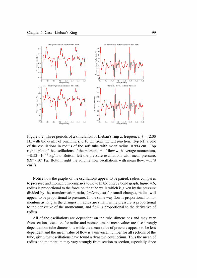
Chapter 5: Case: Liebau’s Ring 99
40.4 40.6 40.8 41 41.2 41.4 41.6 41.8
0.92
0.94
0.96
0.98
1
1.02
1.04
The dynamic radius of a section of the model
Time [seconds]
The
dyn
amic
rad
ius
[cm
]
40.4 40.6 40.8 41 41.2 41.4 41.6 41.8−8
−6
−4
−2
0
2
4
6
8
10
The momentum of the flow in a section of the model
Time [seconds]
The
mom
entu
m o
f the
flow
[kg/
m*s
]
40.4 40.6 40.8 41 41.2 41.4 41.6 41.89.6
9.7
9.8
9.9
10
10.1
10.2x 10
4 The driving pressure in a section of the model
Time [seconds]
The
driv
ing
pres
sure
[Pa]
40.4 40.6 40.8 41 41.2 41.4 41.6 41.8−150
−100
−50
0
50
100
150
200The volume flow in a section of the model
Time [seconds]
The
vol
ume
flow
[cm
3 /s]
Figure 5.2: Three periods of a simulation of Liebau’s ring at frequency, f = 2.06Hz with the center of pinching site 10 cm from the left junction. Top left a plotof the oscillations in radius of the soft tube with mean radius, 0.993 cm. Topright a plot of the oscillations of the momentum of flow with average momentum,−9.52 · 10−2 kg/m·s. Bottom left the pressure oscillations with mean pressure,9.97 · 104 Pa. Bottom right the volume flow oscillations with mean flow, −1.78cm3/s.
Notice how the graphs of the oscillations appear to be paired; radius comparesto pressure and momentum compares to flow. In the energy bond graph, figure 4.6,radius is proportional to the force on the tube walls which is given by the pressuredivided by the transformation ratio, 2π∆xrn, so for small changes, radius willappear to be proportional to pressure. In the same way flow is proportional to mo-mentum as long as the changes in radius are small, while pressure is proportionalto the derivative of the momentum, and flow is proportional to the derivative ofradius.
All of the oscillations are dependent on the tube dimensions and may varyfrom section to section, for radius and momentum the mean values are also stronglydependent on tube dimensions while the mean value of pressure appears to be lessdependent and the mean value of flow is a universal number for all sections of thetube, given that oscillations have found a dynamic equilibrium. Thus the mean ofradius and momentum may vary strongly from section to section, especially since
100 Mathematical Modeling of Flow Characteristics in the Embryonic Heart
the radius of the soft and the rigid tube differs, while mean pressure varies onlylittle depending on the section, with the strongest variance observed in the rigidtube. The mean pressure of the soft tube will be regarded as almost invariant andspecifically reported for the section opposite to the pinching site from the middleof the soft tube.
The mean pressure with 9.97 · 104 Pa is a little lower than the equilibriumpressure, set to atmospheric pressure, P0 = 105 Pa. This may seem counter-intuitive as reduction of volume, or in this case a reduction of radius, is typicallyassociated with an increase in pressure. But this argument only holds if energy islocally contained, instead an increase in pressure will induce an increase in radius,and similarly for decreases; the mean radius is a little lower than equilibriumradius, 0.7 %, thus the mean pressure is a little lower than equilibrium pressure,0.3 %.
But shouldn’t the pressure increase when the pinching compress the tube,where does that missing pressure go? It is converted to kinetic energy throughBernoulli’s equation. The kinetic energy defines the flow oscillations, and themean kinetic energy will define the mean flow. Furthermore with the oscillationsof the flow energy dissipates through the Poiseuille resistance and the curvatureresistance, effectively due to friction.
The mean flow with −1.78 cm3/s is much less compared to the flow oscilla-tions. The total volume inside the ring is 257.6 cm3 at equilibrium so a flow ofnearly 200 cm3/s would mean that the liquid moves almost a full circle in onesecond, though this only lasts for a moment it is clear that it takes a lot of energyto accelerate the liquid to such velocities, energy that is supplied by the pressureoscillations. On the other hand, the mean flow compares to a mean flow veloc-ity, 0.56 cm/s, so even though the oscillations are massive the liquid moves quiteslowly round in the ring.
5.4.3 The no-flow condition
An important condition to test for the model of Liebau’s ring is if the flow is trulyzero when the pinching site is placed symmetrically in the system, ie. centrallyon the soft tube. As explained the Liebau effect is attributed to the mismatchbetween reflected pressure waves in the system, but if the pinching site is placedsymmetrically no mismatch is encountered, and thus no flow.
Therefore a test of the no-flow condition is significant to prove that the modelis in accordance with the simplest physical conditions of the system, or, if not, toinvestigate what could be causing an eventual error.
Figure 5.3 shows the plots of flow and pressure from a simulations using themodel setup described in section 5.2 with the number of sections N = 50 andwith the 3 sections wide pinching site situated in section 12, 13 and 14, which iscentrally on the soft tube of the ring.

Chapter 5: Case: Liebau’s Ring 101
44.4 44.6 44.8 45 45.2 45.4 45.6−250
−200
−150
−100
−50
0
50
100
150
200The volume flow in a section of the model
Time [seconds]
The
vol
ume
flow
[cm
3 /s]
44.4 44.6 44.8 45 45.2 45.4 45.6
9.7
9.75
9.8
9.85
9.9
9.95
10
10.05
10.1
10.15
10.2
x 104 The driving pressure in a section of the model
Time [seconds]
The
driv
ing
pres
sure
[Pa]
Figure 5.3: Three periods of a numerical test of the model with the number of sec-tions N = 50 and the three sections pinching site centered at section 13, midwayson the soft tube. Model setup as defined in section 5.2. Both flow and pressureoscillations are very dramatic, while mean flow is almost zero, 1.67 · 10−4 cm3/s,and mean pressure drops a little compared to atmospheric pressure, 9.97 · 104 Pa.
As the figure demonstrates the mean flow is only 1.67 · 10−4 cm3/s despite therange of oscillations reach from −250 to 200 cm3/s. Clearly this proves that themodel is in accordance with the no-flow condition, the minimal deviation fromzero flow must be attributed to numerical effects in the model or in the computa-tion of the mean.
Additionally figure 5.3 demonstrates a drop in the mean pressure comparedto pressure at time zero, which is set to atmospheric pressure, P0 = 105 Pa. Themean pressure drops to 9.97 · 104 Pa though no mean flow is observed, whichmeans that the mean kinetic energy is zero. This reveals that the greatest leak inpressure actually comes from the Poiseuille and curvature resistances that dissi-pate energy due to the flow oscillations.
An interesting question regarding the no-flow condition is, if the transmittedwave that travels round the ring is capable of inducing flow. Because this wave isindependent of the position of the pinching site it should be able to induce flowwhen the pinching site is positioned symmetrically in the system, if this is thecase.
There are two possible cases that should be tested; the transmitted wave en-counters resonance and the transmitted wave does not encounter resonance. Thelast case is tested in figure 5.3 as the frequency, f = 2.06 Hz does not correspondto any resonance modes of the transmitted wave, no flow is observed in that case.The first case is visible in figure 5.4.
In the figure flow oscillations are visible for transmitted waves with periodscorresponding to once or twice the travel time round the ring, none of them pro-duce any mean flow. Figure 5.3 and 5.4 should be enough to prove that the trans-

102 Mathematical Modeling of Flow Characteristics in the Embryonic Heart
30.2 30.4 30.6 30.8 31−200
−150
−100
−50
0
50
100
150
The volume flow in a section of the model
Time [seconds]
The
vol
ume
flow
[cm
3 /s]
15.1 15.2 15.3 15.4 15.5
−100
−50
0
50
100The volume flow in a section of the model
Time [seconds]
The
vol
ume
flow
[cm
3 /s]
Figure 5.4: Three periods of a numerical test of the model with N = 50 sectionsand the three sections pinching site centered at section 13. Model setup is definedin section 5.2. On the left is a simulation with f = 2.96 Hz, corresponding to thetravel time round the ring equal to the half of a period, yielding a mean flow of6.49 · 10−4 cm3/s. On the right is a simulation with f = 5.95 Hz, correspondingto the travel time round the ring equal to a full period, yielding a mean flow equalto 6.51 · 10−4 cm3/s. Mean flow in both simulations is effectively zero safe fornumerical effects.
mitted wave does not induce flow in the system, the mean flow must come fromthe reflected waves.
Notice how the range of flow oscillations are greater in figure 5.3, lesser in theleft plot of figure 5.4 and least in the right plot. All three plots are made for section20 of a model with 50 sections and with the pinching site centered at section 13,but the oscillations can vary a lot from section to section and depending on thefrequency. The plots in figure 5.4 correspond to modes where the transmittedwave encounters resonance, thus a standing wave is created with antinode at thepinching site, so the full oscillations are not visible in those plots. In the plot offigure 5.3 the frequency does not correspond to any modes of standing waves, so itis a more complicated picture of the transmitted and reflected waves in the system.
5.4.4 The frequency scan
In relation to the Liebau effect the interesting question is how the dynamical flowand pressure oscillations lead to conditions that produce a mean flow round in thering, and how that situation depends upon a number of different factors. As dis-cussed in section 5.3 one of those factors is the frequency of the periodic compres-sions of the tube, which will induce pressure waves in the system and at certainfrequencies these pressure waves will resonate with the periodic pinching mecha-nism, as presented in table 5.1.

Chapter 5: Case: Liebau’s Ring 103
2 4 6 8 10
−4
−3
−2
−1
0
1
2
3The mean flow in the model as a function of frequency
Frequency [Hz]
The
mea
n vo
lum
e flo
w [c
m3 /s
]
Figure 5.5: A frequency scan of the mean flow in the ring with setup as describedin section 5.2. The solid curve represent a series of simulations with much finerresolution in the frequency range that due to long computation time of simulationswith longer periods does not extend all the way to the low frequency range, butas shown by the figure the coarser resolution scan (dotted curve) demonstratesthe features of the frequency spectrum reasonably well. Several of the resonancefrequencies defined in table 5.1 are visible in the graph as small markers in thebottom of the plot; green markers are right reflected waves and yellow are leftreflected waves, the size of the markers refer to the reflection order, and the dashedmarkers refer to j = 2 in table 5.1.
Naturally it will be interesting to investigate exactly how these resonance fre-quencies affect the mean flow for the system. To make a frequency scan of thesystem the program from appendix A is changed so that for any array of frequen-cies it will iterate the equations for 70 periods of time and afterwards calculate themean values by integrating over the last twenty periods and dividing with time,assuming the system have found its dynamic equilibrium at that time. This is notshown in the appendix. This time consuming procedure gives the frequency spec-trum for mean values of rn, pn, Pn and Qn for every frequency in the array, whichis visible in figure 5.5.
As is visible in the figure the mean flow is primarily negative for the frequencyspectrum, that is the flow moves from the larger part of the soft tube towards theshorter part. This corresponds to the assumption that in the low frequency rangethe right reflected pressure waves will generally be dominant, as the distance theyhave to travel is longer and thus their travel time will be better compatible with theperiod of the compressions. At higher frequencies more resonance modes of the

104 Mathematical Modeling of Flow Characteristics in the Embryonic Heart
left reflected waves may come into play such that the distribution between positiveand negative mean flow may be more even.
At certain frequencies the spectrum demonstrate clear peaks where the meanflow is either intensified, nullified or it changes direction, most of these appear tocorrespond roughly to the resonance frequencies identified in table 5.1.
The resonance frequencies of 2.78 Hz, 3.16 Hz, 3.69 Hz, 5.14 Hz and 5.54Hz can be clearly identified, and with some imagination also the resonances at1.70 Hz and 1.83 Hz. The frequencies of 3.16 Hz and 5.54 Hz correspond to theresonance of left reflected waves that change the mean flow to a positive direction.This also helps to identify the resonance at 1.83 Hz, which should be shifted a littlehigher to fit with the graph. The other resonances correspond to right reflectedwaves that increase the mean flow in the negative direction.
Additionally unidentified peaks are visible in figure 5.5, likely correspondingto reflection patterns not identified in section 5.3. Specifically for frequencieslarger than 6 Hz it does not appear as if the identified resonances can explain thegraph of the mean flow.
Furthermore the mean flow is not only dependent on the resonance of pressurewaves with the compression pump, for most parts of the frequency spectrum themean flow is produced from interference between reflected and transmitted pres-sure pulse waves, with the the resonances being situations that are easily identifi-able and should dominate the system at their respective frequencies. The pressurepulse waves have several modes of interference, it is quite possible that severalreflected waves resonates to amplify each other and even if no waves resonate at acertain frequency they will not terminate each other either due to the nature of thepulse waves. Generally at a given frequency it is very difficult to predict the exactvalue of the mean flow from the complicated interaction of pressure waves.
5.4.5 Position of the pinching site
From the premise given in the calculation of the resonance frequencies in table 5.1it is clear that the observed mean flow will depend on the position of the pinchingsite, especially since it is proven in section 5.4.3 that the transmitted pressurewave, which is site-independent, does not produce any mean flow. Thus it willbe interesting to observe how the simulation results change when the position ofthe compression pump is moved. For that reason the program from appendix A ischanged just like in section 5.4.4 though this time the mean values are computedas a function of the position of the pinching site.
Figure 5.6 shows a plot of the mean flow as a function of the position of thepinching site in the ring. One thing that is clear to see in the figure is the symmetrybetween the two halves of each tube, when the pinching site is moved to theopposite site from the middle of the tube flow is reversed but of equal magnitude.

Chapter 5: Case: Liebau’s Ring 105
0 10 20 30 40 50 60−15
−10
−5
0
5
10
15The mean volume flow in any section of the model
Position of the pinching site
Mea
n vo
lum
e flo
w [c
m3 /s
]
Figure 5.6: A set of simulations with N = 60 sections where the pinching sitehas been moved around to any position of two tubes, model setup as described insection 5.2. In the plot the mean flow is visible for frequencies of 2.06 Hz (redcurve), 4.00 Hz (blue curve), 6.00 Hz (green curve) and 8.00 Hz (yellow curve),the dashed part of the curves are reconstructions from other parts of the curves.The dotted lines separate the tubes into four quarters, the first two quarters belongto the soft tube and the other two to the rigid tube. The two black arrows markthe position of the pinching site for all other simulations presented in this thesis,except the ones in section 5.4.3 of course.
One other thing that is clearly visible in the figure is the dependency betweenfrequency and the position of the pinching site. At low frequency it appears thatthere is only one optimal position of the pinching site, about one third of the lengthfrom the junction between the two tubes, but with higher frequencies that optimalposition moves closer to the junctions and other positions appear in relation to theshortening of the wavelength for higher frequencies.
It must be that the site of the compression pump should fit with the distancethat the traveling pressure waves are able to cover in a whole number of periodsgoing from the pinching site to a point of reflection and back, such that the sites ofoptimal mean flow are the positions for which a wave of that frequency encountersresonance in the ring. As such it is clear that the position of the pinching siteselected for all the other simulations, marked by the arrows in figure 5.6, willnot see the maximum Liebau effect possible with the two tubes for the chosenfrequencies.

106 Mathematical Modeling of Flow Characteristics in the Embryonic Heart
In the report by Snitker et al. [2000] it is claimed how positioning the pumpingmechanism exactly at the junction between the two tubes produces the highestmean flow with a frequency, f = 2.06 Hz. From that it is speculated that this willbe the case for all frequencies. While figure 5.6 confirms the first result it alsoproves that for other frequencies the mean flow may be less, even zero.
Positioning the pinching site at the junction between the tubes is a special casebecause it effectively removes one of the possible reflection sites for the waves inthe tube, this completely changes the system and for that reason no more time willbe spent with that case here. Similarly figure 5.6 demonstrate that higher meanflows may be achieved by pressing on the rigid tube, for a pinching mechanismdesigned for pressing the soft tube. This comes only natural since the increasedthickness and elastic module of the rigid tube makes it harder to compress it, inthis way more energy is spent to compress the tube to a compression ratio of 25%, thus the waves in the system contain more energy yielding a higher pressureand displacement amplitude. No more time will be spent on that case either.
With that the basic phenomena in the simulations of Liebau’s ring are pre-sented. In the following focus will be put on a comparison of the simulationresults to other reports and specific elements of the model will be examined to testthe validity, stability and performance of the model.
5.5 Comparison to other results
The simulations of Liebau’s ring are compared to another set of simulations byOttesen [2003] and to experimental measurements by Snitker et al. [2000].
The experiments by Snitker et al. [2000] measures the mean velocity of theflow in Liebau’s ring, specifically pertaining to different compositions of tubematerials and the position of the pump in relation to the junctions between thetubes. The experiments involve an external physical pump that is connected toLiebau’s ring through as small tube, it works by producing an excess volume ofliquid inside the ring, which will then induce the flow. The frequency of the pumpis 2.06 Hz in all reported experiments.
The simulation results by Ottesen [2003] are based on a one-dimensional av-eraging of the Navier-Stokes equations into a system of differential equations,which are solved using the eigenvalue method and simulated using Richtmeyer’stwo step version of Lax-Wendroff’s method. The pumping mechanism used inthese simulations is described in equation 5.1 and simulation results are specifi-cally reported for the frequency range from 2.5 Hz to 3.5 Hz.
The setup and pinching mechanism of Ottesen is the same as used for thesimulations of Liebau’s ring here, so results will be comparable to the extendthat in the data by Ottesen the system is subjected to a small pressure increasebefore starting the pumping mechanism. This high pressure should not have much

Chapter 5: Case: Liebau’s Ring 107
2.5 3 3.5
−3
−2.5
−2
−1.5
−1
−0.5
0
0.5
1
1.5
2
The mean flow in the model as a function of frequency
Frequency [Hz]
The
mea
n vo
lum
e flo
w [c
m3 /s
]
Cr = 25%Cr = 50%SimulationsCr = 25%SimulationsCr = 25%SimulationsCr = 50%
Figure 5.7: Comparison of the mean flow from the simulations of Liebau’s ringto data from Ottesen [2003] (square and triangle plots). The simulations are madewith N = 60 and setup as described in section 5.2, though one set is made withcompression ratio c = 25 % (solid and dash-dotted curve as presented in figure5.5) and another is made with compression ratio c = 50 % (dashed curve).
influence on the observed Liebau effect as demonstrated in section 5.5.1.Figure 5.7 shows a comparison between mean flow of the simulations to data
supplied in by Ottesen [2003]. The figure compares the mean flow for simulationswith a compression ratio 25 % and 50 %, where the compression ratio is definedby the compression of cross-sectional area, c = A0−Amin
A0, according to the setup
in section 5.2.There seem to be good correspondence between the registered mean flow from
the two sets of simulation data when the compression ratio, c, is set to 25 %, tothe point that deviances can be ascribed to difference in modeling and simulationprocedure. Both sets of data has mean flow about −1.0 to −1.5 cm3/s for mostparts of the frequency range, but in the vicinity of 2.79 Hz, 2.97 Hz and 3.17 Hzsomething happens, corresponding to resonance modes defined in table 5.1.
For the compression ratio, c, set to 50 % the comparability is more unclear.The mean flow is still in the vicinity of −1.0 to −1.5 cm3/s in the low and highfrequency end while something else happens in the frequency band around 3.0 Hz.The mean flow by Ottesen appear to change direction around the resonances in thisinterval, which is also the case in the simulations of the model, though not in thesame way. It appears as if the simulations at c = 25% have good comparability,yet the lack of data points makes comparison uncertain for higher compressionrates.

108 Mathematical Modeling of Flow Characteristics in the Embryonic Heart
Comparison to the results by Snitker et al. [2000] is more complicated. Theirexperiment consisted of two tubes clamped together and an external pump setinto the system through a T-junction and a third tube. The pump consists of acompliant plastic bag that is periodically compressed to pump an excess volumeinto the system, and through the compliance of the bag it is gradually refilled suchthat the total volume of liquid pumped into the system during one period is zero.
The pump employed in this experiment has an active duration of 1/4 of theperiod and a relaxation duration of 3/4 of the period, the frequency is set to 2.06Hz for all measurements, and the excess volume pumped into the system the ac-tive duration is estimated between 10 - 12 cm3. Unfortunately Snitker et al. [2000]fail to measure compliance of the pump, so a reconstruction will not be attemptedhere. It is however possible to make a crude modification of the pumping mecha-nism in the model to compare with Snitker, such that an excess volume is period-ically injected and removed not relying on compliance, using the equation,
V (t) = Vtotal
(1− cos
(2π
τt))
, (5.11)
for (t mod T ) ∈ [0, τ [ and V (t) = 0 else, where τ it the active duration asa fraction of the period and Vtotal is the total volume of fluid pumped into thesystem during the active duration.
The excess volume is added to the volume flow between two sections of themodel as a function of time by means of its derivative,
dV
dt= Vtotal
2π
τsin
(2π
τt), (5.12)
for (t mod T ) ∈ [0, τ [ and dVdt
= 0 else.The excess volume pump periodically injects a volume of 10 - 12 cm3 into
the system, correspondingly the pinching mechanism defined by equation 5.2 andimplemented into a model with N = 60 sections while the pinching site is 3sections wide compresses the tube with a volume of 3.2 cm3 for a compressionratio of 25 % and with a volume of 6.3 cm3 with a compression ratio of 50 %. Thepinching mechanism needs to compress the tube with a compression ratio of 80% or more to compare with the excess volume pump.
Snitker et al. [2000] measure the flow velocity in the ring by timing the move-ment of small plastic balls suspended in the water inside the tubes, specifically inthe rigid PVC tube, which is transparent. Explained in the report is the concern tofind a material for the plastic balls that would remain suspended in the liquid andneither sink or float, eventually folded pieces of plastic bags was used. Due to thevolume of the plastic balls compared to the velocity profile the balls will experi-ence a velocity gradient and thus they will tend to migrate towards the center ofthe tube where the velocity is highest in an effect similar to the one encountered

Chapter 5: Case: Liebau’s Ring 109
by blood cells [Meier, 1987], though the rugged shape of the folded pieces ofplastic could disrupt this migration at times. Thus it is expected that the velocitymeasured by Snitker et al. [2000] is the peak velocity inside the tube.
Assuming the flow has a Poiseuille velocity profile the measured velocity cor-responds to the mean volume flow,
Q = 2π∫ R
0Vmax
(1− r2
R2
)r dr =
πR2
2Vmax, (5.13)
which is half of the volume flow achieved under the assumption of a flat velocityprofile. The flow however has a Womersley velocity profile, which means that thecorresponding flow lies in the interval from 1
2πR2Vmax to πR2Vmax.
From an experiment involving two tubes as described in section 5.2 and with avolume pump positioned 10 cm from the left junction Snitker et al. [2000] obtaina flow velocity equal to 5.0± 0.5 cm/s, corresponding to a flow from 5.0± 0.5 to10.0± 1.0 cm3/s.
Correspondingly simulations with the pinching mechanism from section 5.2yield mean flows of −1.78 cm3/s, −1.31 cm3/s and −0.92 cm3/s for compressionratios of 25 %, 50% and 75 % respectively. And for a simulation with the abovesetup and an excess volume pump as suggested by equation 5.12 a mean flowof 3.1 cm3/s is obtained if the activity duration is set to one tenth of the periodas suggested by Ottesen [2003] while a mean flow of only 0.3 is obtained if theactivity duration is set to one fourth of the period, much lower than the measuredflow rate.
5.5.1 High pressure results
The results by Snitker et al. [2000] were achieved for a system with high pres-sure, obtained by injecting 10 or 20 cm3 of liquid into the system and letting itrelax before setting the liquid into motion with the volume pump. It is reportedthat the system would not function satisfactory with atmospheric pressure, as thevelocities measured had a large spread in magnitude and did not demonstrate anysystematic behavior.
To compare with those results a set of simulations are prepared where a singlesection of the tube is dilated to accommodate either 10 or 20 cm3 of extra volume,and the system is allowed to relax such that all the sections of the model will havea slightly dilated radius compared to equilibrium radius. When the system hasfound its new stable condition the pumping mechanism is started with the use ofthe excess volume pump from equation 5.12. A comparison of flow and pressureof three simulations involving 10 cm3 extra volume, 20 cm3 extra volume, and noextra volume is visible on figure 5.8.

110 Mathematical Modeling of Flow Characteristics in the Embryonic Heart
40 40.2 40.4 40.6 40.8
−100
−50
0
50
100
The volume flow in a section of the model
Time [seconds]
The
vol
ume
flow
[cm
3 /s]
40 40.1 40.2 40.3 40.4 40.5 40.6 40.7 40.80.99
0.995
1
1.005
1.01
1.015
1.02
1.025
1.03x 10
5 The driving pressure in a section of the model
Time [seconds]
The
driv
ing
pres
sure
[Pa]
Figure 5.8: A comparison of simulations with the excess volume pump at fre-quency f = 2.06 Hz: One simulation without higher pressure (solid curve), onesimulation with 10 cm3 extra liquid volume (dashed curve) and one with 20 cm3
extra volume (dash-dotted curve), the increased volume before the onset of theexcess volume pump will increase the equilibrium pressure inside the tube. Onthe left is a plot of the volume flow oscillations; all three simulations follow thesame curve, except that amplitude increases with the higher pressure. On the rightis a plot of the pressure oscillations; the curves are nearly identical, except thatthe higher pressure shifts the curve towards higher values.
As the figure demonstrates the simulations at higher pressure are not reallythat different from the normal simulation: The amplitude on the flow oscillationsincrease with higher pressure, and the pressure oscillations are naturally shiftedtowards higher pressure.
It is noticeable on figure 5.8 that the mean pressure is almost constant underthe application of the excess volume pump, while it decreases under the use ofthe pinching mechanism explained in section 5.2. For the simulations with 0, 10and 20 cm3 extra volume the mean pressure is 1.0001 · 105 Pa, 1.0131 · 105 Pa and1.0197·105 Pa respectively, while the corresponding equilibrium pressures are 105
Pa, 1.0119 · 105 Pa and 1.0199 · 105 Pa. The differences between equilibrium andmean pressures are 100 Pa or less with a tendency to increase rather than decrease,this may be an indication that the two pumping mechanisms are not comparableat all.
A further comparison of the mean flow produced by the excess volume pumpto that produced by the pinching mechanism and the data by Ottesen [2003] is vis-ible on figure 5.9. Furthermore the reported flow velocities by Snitker et al. [2000]are drawn on the figure as vertical bars, calculated into volume flow through equa-tion 5.13. It is clear that flow corresponding to the observed velocities is muchlarger than any computed flow from the models.
According to Snitker et al. [2000] the difference between experiments with 10

Chapter 5: Case: Liebau’s Ring 111
2 2.5 3 3.5 4
−2
0
2
4
6
8
10
The mean flow in the model as a function of frequency
Frequency [Hz]
The
mea
n vo
lum
e flo
w [c
m3 /s
]
Ottesen [2003]Pinching pump (25%)Excess volume pump no extra volume
Excess volume pump 10 cm3 extra volume
Excess volume pump 20 cm3 extra volume
Figure 5.9: Comparison of the mean flow from the simulations with the excessvolume pump with those of the pinching mechanism (red dotted curve) and datafrom Ottesen [2003] (black dotted curve) and the reported velocities from Snitkeret al. [2000] calculated into an interval for the volume flow. The black bar is thevolume flow for their experiment with 10 cm3 extra volume of liquid, rangingfrom 5.0 to 10.0 cm3/s, and the gray bar is the volume flow for their experimentwith 20 cm3 extra volume of liquid, ranging from 4.7 to 9.4 cm3/s. Though itis demonstrated that the excess volume pump is capable of producing flow in therange reported by Snitker et al. [2000] explicitly at f = 2.06 Hz it produces nearlyno flow at all.
and 20 cm3 extra volume injected prior to the start of the pumping is a decrease invelocity for the higher pressure measurement, though for other of their measure-ments the higher pressure demonstrates a higher velocity. Generally that picture isconfirmed here, the simulation with 20 cm3 extra volume constituting higher pres-sure will sometimes exhibit a lower mean flow and sometimes a higher, comparedto the other simulations. In figure 5.9 this is proved to be dependent on frequency,but it may as well depend on a number of other things, for instance the position ofthe pump on the ring, which seems to be the case for Snitker et al. [2000].
The frequency spectrum demonstrated for the simulations with the excess vol-ume pump does not particularly resemble that of the pinching mechanism, in someways they appear to be mirror images of each other, but the most notable peak ofthe excess volume spectrum at f = 3.5 Hz is not recognized in the spectrum of thepinching mechanism. Furthermore it appears there is a minor peak at f = 2.06Hz for the simulations at higher pressure, which is not observed for any of thesimulations involving the pinching mechanism.
Many things point to the fact that the pumping mechanisms are fundamentally

112 Mathematical Modeling of Flow Characteristics in the Embryonic Heart
different and incomparable, it has been reported many times for instance by Otte-sen [2003] that the observed Liebau effect depends on the method of pumpingapplied, which is confirmed by figure 5.9. In fact according to Yang and Wang[2010] valveless systems that differ in configuration or operation conditions (downto the frequency of compression) may rely entirely upon different mechanisms topump fluids.
The excess volume pump involved in the simulations is a very poor resem-blance of the pump applied by Snitker et al. [2000] due to the fact that the simu-lated pump actively refills instead of passively though its compliance, in the sim-ulations the pump interacts with the tube by ‘magically’ introducing an excessvolume in the tube while the real pump has a whole other range of interactionpossibilities not accounted for by the model.
Constructing a hybrid pumping mechanism that works like the excess volumepump but with the activity duration of the pinching mechanism (1/10 of the periodinstead of 1/4 of the period) does not improve the comparison, even through thehybrid pump will produce 10 cm3 excess liquid volume for only one tenth ofthe period corresponding to the pinching mechanism with an 80 % compressionratio, which compress a volume equal to 1.01 cm3 for one tenth of the period.The spectrum of the mean flow mostly resembles that of the other excess volumesimulations, but with more modes of resonance. Thus the difference in pumpingmechanisms can not be explained only by the difference of activity duration.
The conclusion is that the model is not able to reproduce the data from Snitkeret al. [2000], mainly out of a lack of information about the pumping mechanismused in the experiment. Many things are unclear about the experiment: the esti-mation of elastic modulus of the wall of the tubes, the estimation of mean velocitybased on the timing of plastic balls in the liquid, disturbance of momentum oscil-lations by the plastic balls, which could produce a more smooth mean flow, but inthe end it all comes down to the pumping mechanism. The pumping mechanismis extremely important for the observed Liebau effect to the point that it is almostimpossible to compare two cases if not the pumping mechanisms are comparable.
5.6 Testing model parts
One huge advantage of the application of energy bond networks in the modelingis the possibility to add or remove effects in the model just as a set of buildingblocks. This makes it very easy to construct tests of the model to estimate theimportance of different model elements.
Chapter 5: Case: Liebau’s Ring 113
The model is constructed in basically two steps; one step involving the fun-damental elements of elastic compliance, liquid inertia and flow resistance, andanother step involving three additional elements of the model: Womersley theory,shear forces in the tube and curvature of the tube. As these three last elementscarry additional assumptions about the behavior of the flow and elasticity of thetube and sometimes deliberately are left out in reports of valveless flow models,see for instance [Manopoulos et al., 2006] or [Azer and Peskin, 2007], it will beinteresting to inspect what influence the elements or their absence will have on thesimulations of Liebau’s ring.
5.6.1 Womersley theory
Many reports point to the assumption that Womersley theory does not have muchinfluence on the flow, for instance Azer and Peskin [2007] state that the resultsof their simulations involving Womersley theory are similar to other models as-suming other shapes of the velocity profile, though some simulations may showgreater effect of the velocity profile, specifically if they involve a Poiseuille ve-locity profile. In a similar fashion Manopoulos et al. [2006] argue that for highWomersley numbers the inertia correction factor, ψ, is close to unity and in orderto eliminate parameters from their model they assume ψ = 1 in all their simula-tions.
With frequencies in the range from 1 to 5 Hz and the model setup describedin section 5.2 the real values of the inertia correction factor lies in the range from1.07 to 1.03, thus ψ = 1 is a fair simplification of this model, though not ingeneral. On the other hand setting ψ = 4/3 in assumption of a Poiseuille profilemay be interesting for the model, figure 5.10 shows a comparison of simulationsinvolving a standard Womersley profile, a flat profile, ψ = 1, and a Poiseuilleprofile, ψ = 4/3.
From the figure it is clear that the difference in results between simulationswith a regular Womersley profile and with a flat velocity profile, ψ = 1, areminimal. The results obtained with at Poiseuille profile, ψ = 4/3, are differentfrom the other two. It is clear from the left plot of figure 5.10 that the liquid hashigher inertia as the oscillations are slower, for each period the graph appears toskip an oscillation compared to the other two. On the right plot of figure 5.10 it isvisible that the mean flow of the Poiseuille profile follows the same general curveas the other two, it is only shifted to lower frequencies. This is not coincidental,in fact equation 5.5 states how the velocity of the pressure wave depends on ψ andthe resonance frequencies are generally proportional to this velocity, therefore the
whole spectrum of the simulations are multiplied with a factor,√1/ψ =
√3/4 ≈
0.87.

114 Mathematical Modeling of Flow Characteristics in the Embryonic Heart
40 40.2 40.4 40.6 40.8 41 41.2−150
−100
−50
0
50
100
150
200The volume flow in a section of the model
Time [seconds]
The
vol
ume
flow
[cm
3 /s]
2 2.5 3 3.5 4
−3
−2.5
−2
−1.5
−1
−0.5
0
0.5
The mean flow in the model as a function of frequency
Frequency [Hz]
The
mea
n vo
lum
e flo
w [c
m3 /s
]
Figure 5.10: A comparison of simulations with different configuration of the iner-tia correction factor: regular Womersley profile (solid curve), flat velocity profile(dashed curve), and Poiseuille profile (dash-dotted curve). On the left is a plotof the oscillations of flow, f = 2.06 Hz, it is visible how the flat profile andthe Womersley profile produce almost similar results, while the oscillations areslower for the Poiseuille profile due to higher inertia. On the right is a plot of themean volume flow, once again the flat profile and Womersley profile are in goodaccordance while the Poiseuille profile is not, if however the plot of the Poiseuille
profile is scaled with a factor,√4/3, towards higher frequencies (as marked by the
arrow) it is seen that the shape of the new dotted curve is in much better agreementwith the other two.
Generally Womersley theory does not mean much for the magnitude of thesimulations of pulsating flow it does however have an effect on oscillations andthe frequency spectrum of the mean flow.
5.6.2 Shear tensions
In the model the shear strain between tube sections are added as an ad hoc im-provement to the model in order to include longitudinal shear effects in the tube.In section 4.3.1 it is explained how these effects are modeled through the use of acapacitor representing shear elasticity and an impedance representing energy lossin the tube wall.
The elements were added to the model after preliminary investigations provedthat a single-capacitance elasticity did not produce accurate results for the model,as such they represent several effects in the model of the tube. Naturally the sim-plest effect is the binding of sections to their neighbors such that the deformationof each section is not independent, physically the elements represent a longitudi-nal stress-strain relation coming from the fact that the tube will attempt to mini-mize length stretches of surface area resulting from the dilation or contraction of

Chapter 5: Case: Liebau’s Ring 115
40 40.2 40.4 40.6 40.8−150
−100
−50
0
50
100
150
200
The volume flow in a section of the model
Time [seconds]
The
vol
ume
flow
[cm
3 /s]
2 2.5 3 3.5 4−6
−4
−2
0
2
4
6
8
The mean flow in the model as a function of frequency
Frequency [Hz]
The
mea
n vo
lum
e flo
w [c
m3 /s
]
Figure 5.11: A comparison of simulations with normal shear effects (solid curve),shear effects with no damping (dashed curve), and no shear effects at all (dash-dotted curve). On the left is a plot of the oscillations of volume flow at frequencyf = 2.06, it is clear how the simulations without damping or shear effects expe-rience much wilder oscillations. On the right is a plot of the mean volume flowas a function of frequency, it is interesting how the simulations without dampingor shear effects seem to follow each other at low and high frequencies, while fre-quencies near the resonances of 2.79 Hz, 2.97 Hz and 3.17 Hz seem to separatethe two curves.
tube sections, and through the energy loss the elements model the fact that thetube walls are not ideally elastic, energy is lost in the wall due to internal friction.
With the shear capacity described as in equation 4.26, Csn = ∆x
2πGh√RnRn+1
,
where G = E/3 is the shear modulus, and the model setup as detailed in section5.2 the values of the capacity areCsn = 1.94·10−3 m/N for the soft tube andCsn =0.77 · 10−3 m/N for the rigid tube. With the maximum dilation-distance betweentwo sections equal to 1.3 mm as described in section 5.4.2 for a simulation withfrequency f = 2.06, the capacity yields a maximum force equal to 0.67 N for thesoft tube and 1.69 N for the rigid tube. For comparison the capacitance reactingto radial expansion of a section yields 2.79 N for the soft tube and 10.98 N forthe rigid tube for the same dilation. Thus the shear forces are between 1/7 to 1/4weaker than the radial forces.
Additionally the impedance, defined as Zsn = T/Csn where T = 0.01 s isthe period of eigenfrequencies in the combination of capacitance and impedanceadded to the model with inclusion of the shear effects. Zsn yields a resistanceequal to 0.52 · 103 N·s/m for the soft tube and 1.30 · 103 N·s/m for the rigid tube,depending on the speed of radius oscillations of the neighboring sections the im-pedance will produce a force to dampen the oscillations.

116 Mathematical Modeling of Flow Characteristics in the Embryonic Heart
35 35.1 35.2 35.3 35.4 35.5 35.6 35.7−150
−100
−50
0
50
100
150
200
The volume flow in a section of the model
Time [seconds]
The
vol
ume
flow
[cm
3 /s]
35 35.1 35.2 35.3 35.4 35.5 35.6 35.79.6
9.7
9.8
9.9
10
10.1
10.2
x 104 The driving pressure in a section of the model
Time [seconds]
The
driv
ing
pres
sure
[Pa]
Figure 5.12: A comparison of simulations at frequency f = 2.75 Hz with normalshear effects (solid curve), shear effects with no damping (dashed curve), andno shear effects at all (dash-dotted curve). On the left is a plot of the flow, thewildness of the oscillations is confirmed, which makes it very hard to determinewhat causes the big difference in mean velocities at the frequency. On the right is aplot of the pressure, which similarly project wildness when undamped or withoutshear effects, the oscillations of the two curves are almost identical and follows thepressure curve of the normal simulation. However, their mean pressure is closerto the equilibrium value than for the normal simulation. From this it would appearthat it is the damping effect that matters most for the oscillations of pressure.
Figure 5.11 and 5.12 shows graphs of three simulations: one simulation withnormal shear effects included, one simulation without shear impedance, Zsn = 0,and one simulation with both shear capacitance and impedance removed, the latteris achieved by setting Csn = 1010 m/N such that the shear effect will be nearlynon-existent.
The figures demonstrate how the oscillations of volume flow and pressure be-come wilder when the impedance or the shear effect is removed; both the am-plitude and number of oscillations per period increase. The oscillating curves ofthe simulations without damping and without shear effects appear to follow eachother for most of the period and it is unclear what exactly causes the major dif-ference in mean flow between the two, at f = 2.75 Hz the simulation withoutdamping has a mean flow of −4.96 cm3/s while the other has a mean flow of 7.25cm3/s.
The mean flow of the simulations without damping and without shear effectsare almost in complete agreement for low frequencies until f = 2.25 Hz andagain for high frequencies from f = 3.50 Hz and up. In the intermediate rangethe simulation without shear effects remain with a high positive mean flow whilethe other becomes negative and almost seems to follow the curve of the regularsimulations with shear effects included. In that intermediate frequency range at

Chapter 5: Case: Liebau’s Ring 117
least three resonance frequencies have been determined at 2.79 Hz, 2.97 Hz and3.17 Hz, it appears as if the simulation without damping is strongly reacting tothose resonances while the other is almost not affected. This makes sense as thepressure wave travels as a function of the elasticity of the tube, when the shearelasticity is removed from the model the circumstances for the pressure wave ischanged dramatically, on the other hand when only the damping is removed theeffect of the pressure wave resonances will be seen much clearer.
The shear effect may be implemented as an ad hoc addition to the model, butit models a real physical effect in the tube; the longitudinal elasticity, which is notcovered by the standard radial elasticity in the model. The longitudinal elastic-ity is important for the propagation of pressure waves in the system. Moreoverthe damping of oscillations in the wall models a real effect of friction in the tubegenerating heat from the oscillations, thereby higher frequency oscillations aredamped, which seem to be the defining discrepancy between curves of the pres-sure oscillations. From figure 5.11 and 5.12 it is clear to see that both dampingand shear elasticity has a major effect on the simulations.
5.6.3 Tube curvature
Curvature of the tubes in Liebau’s ring is a condition that is quite obvious; ofall the cases proposed by Gerhart Liebau in his papers Liebau’s ring is not thesimplest, yet because of the curvature of the ring it is an interesting case for thismodel.
Curvature adds another resistance to the flow but this resistance does not onlydepend on the radius, as is the case for the Poiseuille resistance, it also dependson the momentum of the flow. For flow of small momentum the impedance isinsignificantly small an may be ignored but for flow of higher momentum it maybecome more influential than the Poiseuille resistance.
For pulsatile flow the resistance depends on the oscillations of momentum,which may be important for the Liebau effect as the flow momentum is the integralof the pressure wave. It is however common to ignore the effects of curvaturein models of Liebau’s ring, it is for instance done by both Ottesen [2003] andManopoulos et al. [2006].
The resistance due to curvature is defined in equation 4.38 and while the coef-ficients αKBfT/ψ adds up to 0.38 for the soft tube and 0.49 for the rigid tube andmomentum oscillations have a magnitude of about 10 kg/m·s the relation definedby the radii of the tube yields 7.96 ·104 m−3 for the soft tube and 1.55 ·105 m−3 forthe rigid tube, which can make the resistance explode at times of high numericalmomentum.

118 Mathematical Modeling of Flow Characteristics in the Embryonic Heart
40 40.2 40.4 40.6 40.8−10
−5
0
5
10
The momentum of the flow in a section of the model
Time [seconds]
The
mom
entu
m o
f the
flow
[kg/
m*s
]
40 40.2 40.4 40.6 40.810
1
102
103
104
105
106
Comparison of resitances for a section of the model
Time [seconds]
The
flow
res
ista
nce
[Pa*
s/m
3 ]
Figure 5.13: On the right is a comparison of the momentum of simulations withnormal implementation of curvature (solid curve) and without curvature resistance(dashed curve) at frequency f = 2.06 Hz, it is clear how the oscillations withoutcurvature resistance express a larger amplitude. On the right is a comparison of thePoiseuille resistance (solid curve) to the curvature resistance (dashed curve) for astandard simulation at f = 2.06 Hz (notice the logarithmic axis), the curvatureresistance increase and decrease in relation to the oscillations of the momentum,while the Poiseuille resistance is much more stable.
Figure 5.13 and 5.14 show the comparison of two types of simulations: onenormal simulation with curvature resistance included and another one withoutcurvature, effectively achieved by setting the bending angle of each section tozero.
The figures demonstrate how the resistance due to curvature is much moredynamic compared to the Poiseuille resistance. The resistance from curvatureincreases and decreases in accordance with the numerical value of the momentumof flow but most of the time it is larger than the Poiseuille resistance, sometimeseven with a factor 10 or more.
The damping of the curvature has a large effect on the oscillations of all thevariables of the simulation; the amplitude is decreased yet the shape of the curveis almost similar for simulations with and without curvature, for the flow and themomentum without curvature the curves are shifted to higher or lower values de-pending on the frequency compared to the curves of normal flow and momentum,which creates a dramatic effect for the mean flow, especially in the vicinity ofresonance frequencies. It is possible to identify resonances from table 5.1 at 2.79- 3.17 Hz, 5.13 Hz, 9.50 Hz and possibly also at 1.71 Hz though it is unclear whathappens at the lower frequencies.
It is clear that the curvature of the tube has a large effect on the oscillating flowand pressure waves of the model, and that it is very important for the observationof Liebau phenomena in the tube. Without the curvature the observed Liebau
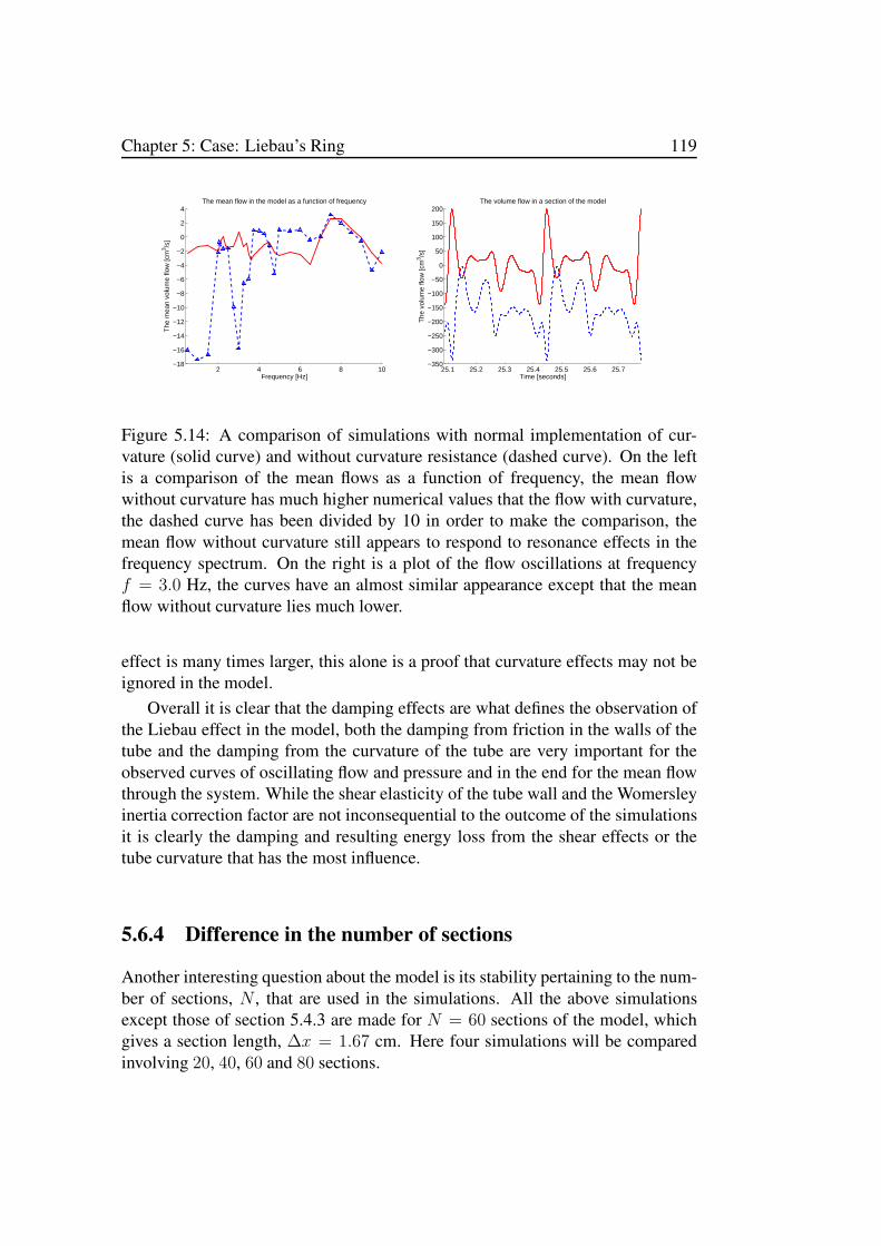
Chapter 5: Case: Liebau’s Ring 119
2 4 6 8 10−18
−16
−14
−12
−10
−8
−6
−4
−2
0
2
4The mean flow in the model as a function of frequency
Frequency [Hz]
The
mea
n vo
lum
e flo
w [c
m3 /s
]
25.1 25.2 25.3 25.4 25.5 25.6 25.7−350
−300
−250
−200
−150
−100
−50
0
50
100
150
200The volume flow in a section of the model
Time [seconds]
The
vol
ume
flow
[cm
3 /s]
Figure 5.14: A comparison of simulations with normal implementation of cur-vature (solid curve) and without curvature resistance (dashed curve). On the leftis a comparison of the mean flows as a function of frequency, the mean flowwithout curvature has much higher numerical values that the flow with curvature,the dashed curve has been divided by 10 in order to make the comparison, themean flow without curvature still appears to respond to resonance effects in thefrequency spectrum. On the right is a plot of the flow oscillations at frequencyf = 3.0 Hz, the curves have an almost similar appearance except that the meanflow without curvature lies much lower.
effect is many times larger, this alone is a proof that curvature effects may not beignored in the model.
Overall it is clear that the damping effects are what defines the observation ofthe Liebau effect in the model, both the damping from friction in the walls of thetube and the damping from the curvature of the tube are very important for theobserved curves of oscillating flow and pressure and in the end for the mean flowthrough the system. While the shear elasticity of the tube wall and the Womersleyinertia correction factor are not inconsequential to the outcome of the simulationsit is clearly the damping and resulting energy loss from the shear effects or thetube curvature that has the most influence.
5.6.4 Difference in the number of sections
Another interesting question about the model is its stability pertaining to the num-ber of sections, N , that are used in the simulations. All the above simulationsexcept those of section 5.4.3 are made for N = 60 sections of the model, whichgives a section length, ∆x = 1.67 cm. Here four simulations will be comparedinvolving 20, 40, 60 and 80 sections.

120 Mathematical Modeling of Flow Characteristics in the Embryonic Heart
18.2 18.4 18.6 18.8 19
−150
−100
−50
0
50
100
150
200
The volume flow in a section of the model
Time [seconds]
The
vol
ume
flow
[cm
3 /s]
18.2 18.4 18.6 18.8 19
9.65
9.7
9.75
9.8
9.85
9.9
9.95
10
10.05
10.1
10.15
10.2x 10
4 The driving pressure in a section of the model
Time [seconds]
The
driv
ing
pres
sure
[Pa]
Figure 5.15: A comparison of simulations involving 80 sections (solid curve), 60sections (dashed curve), 40 sections (dash-dotted curve) and 20 sections (dottedcurve) at frequency f = 2.06 Hz. On the left is a plot of the flow oscillations, somedifferences are visible between the simulations, especially for the simulation with20 sections. On the right is a plot of the pressure oscillations, some differences,especially for for the simulation with 20 sections, are also visible here. However,as the horizontal line indicates the mean pressure is the same for all simulations,9.97 · 104 Pa.
When changing the number of sections it is simultaneously needed to changethe position of the pinching pump and how many sections it covers. For the sim-ulation involving 60 sections the pinching site is 3 sections wide and centered onthe sixth section from the left. Naturally the pinching site will be 1, 2 and 4 sec-tions wide for the simulations involving 20, 40 and 80 sections, while the positionof the site is at section 2 for the simulation involving 20 sections, at section 4and 5 for the simulation involving 40 sections, and at section 7, 8, 9 and 10 forthe simulation involving 80 sections. The positions of the pinching site does notcorrelate completely for the four simulations.
Figure 5.15 shows a comparison of the four simulations through graphs ofthe oscillations of flow and pressure. It is visible how the curves in both graphsgenerally follow the same path but with minor deviations mostly at the peak of theoscillations, especially the curve for the simulation involving 20 sections seems todeviate from the others.
The mean pressure is similar for all the simulations, 9.97 · 104 Pa, but that isnot the case for the mean flow: the calculations of the mean flow yielded 2.67cm3/s, −2.86 cm3/s, −1.78 cm3/s and −4.01 cm3/s for the simulations involving20, 40, 60 and 80 sections respectively.
The large differences in mean flow between the simulations may seem dis-heartening for the model stability but it is explained with the differences in com-pression profile. As defined by equation 5.3 the compression profile defined by

Chapter 5: Case: Liebau’s Ring 121
the minimum radius for each section of the pinching site depends on the numberof sections included in the pinching site, which again depends on the number ofsections included in the model, as it is the intention that the pinching site coversone tenth of the soft tube comparative to [Ottesen, 2003].
Therefore the compression profile will look different for each of the four sim-ulations: For the first two it will be a square profile, for the third and fourth sim-ulation it will be a staircase. Generally the more sections in the pinching site thebetter it will approximate a sinusoidal profile.
Ottesen [2003] reports a preliminary investigation that showed that the com-pression profile and the speed of the compressions are very influential to the di-rection and magnitude of the observed mean flow, which seems to be the casehere.
Furthermore the compressed volume is different for each simulation; for thesimulations involving 20, 40, 60 and 80 sections the compressed volume equalsto 3.9 cm3, 3.4 cm3, 3.2 cm3 and 3.0 cm3 respectively. As this is the volume thatis displaced by the pinching mechanism it will probably have some influence onthe mean flow, though it does not appear to be in any systematic way.
Finally the numerical calculation of the mean flow may experience higher un-certainties when the number of sections is reduced. Already the computation ofthe mean relies on an algorithm to find an exact number of periods in the time-data, which are not spaced with equal time steps, and a numerical integration ofthe data for each of the variables based on a mean between right and left Riemannsums. Possibly this procedure becomes unstable with less sections in the model.
Though based on figure 5.15 it is seen that the oscillations follow the samegeneral curves, which is an indication that the dynamics in the system is the sameindependent of the number os sections. Naturally more sections would producebetter results, however the computation time is longer and even more problematic,a simulation with too many sections produce too much data for the computer tohandle.
5.7 Conclusion to the case of Liebau’s ring
The results of the simulations of Liebau’s ring did not produce an exact validationof the cylindric model. As indicated by the comparison of results Liebau’s ring is acomplicated case where many different factors have influence on the observationsof the Liebau effect; from the material properties of the tube to the frequency,shape and position of the pumping mechanism down to the very way the model isbuilt.

122 Mathematical Modeling of Flow Characteristics in the Embryonic Heart
Though it was not possible to reproduce data from Snitker et al. [2000] and thesimulations by Ottesen [2003] only partially agree with the simulations using thepinching mechanism with compression ratio at 25 % and 50 %, the explanationfor the discrepancies is clear; it all lies in the pumping mechanism, even for thecomparison with the simulation data by Ottesen [2003] the pinching mechanismis only an approximation and as demonstrated in section 5.6.4 even pinching siteswith different number of sections are hard to compare. Because the pumpingmechanisms are not comparable it is only possible to make a partial comparisonof experimental and simulation data.
On the other hand the simulations of Liebau’s ring demonstrate the strengthsof the cylindric model and the way it is built. Because of the modular constructionof the model it is possible to compare the effect of different additions to the modeland decide how they each influence the observation of flow and pressure in themodel. It is clear from those observations that the impedance in the model has avery large influence on the observed Liebau effect.
All in all the simulations of Liebau’s ring makes it clear that the model isable to handle complicated flow phenomena, that would not be possible with aWindkessel or transmission line model. The difference is that the Liebau effectis a non-linear phenomenon that would not be visible in a linear model, and eventhough the cylindric model is built from the principle of linear response theoryinherent in the energy bond technique the composition of elements and transfor-mations in the model grants it non-linear qualities.
Chapter 6
Construction of the Eccentric Tube
Models
In this chapter the model constructed in chapter 4 will be expanded to have anelliptic cross-section, and by the end of the chapter to a layered model with anelliptic inner layer and circular outer layer following the observations of section2.3.
The models herein will be referred to as the elliptic model, as the first modelhas an elliptic cross-section, and the embedded model, since the final step of themodeling procedure will be as an elliptic tube embedded inside a cylindric. Oc-casionally they may also be referred to as the eccentric models because elasticcompliance and cross-sectional contraction are eccentric, as opposed to concen-tric compliance and cross-sectional contraction, which is the case for the modelpresented in chapter 4.
The modeling procedure in this chapter follows the same basic steps as inchapter 4 on the basis of the energy bond theory; at first the fundamental elementsof elasticity, inertia and impedance are defined, then additional content of shearforces, tube curvature and Womersley theory is included and the characteristicequations of the model are derived, finally as an extra step in the modeling pro-cedure in this chapter the embedded model will be constructed as an additionalstructure for the elliptic model.
6.1 The ellipse
An ellipse can be described by its major and minor semi-axis, a and b respectively,when a = b the ellipse becomes a circle. A parameter describing an ellipse’sdeviance from a circle is known as the eccentricity,
123

124 Mathematical Modeling of Flow Characteristics in the Embryonic Heart
ǫ =
√a2 − b2
a2=
√√√√1−(b
a
)2
, (6.1)
the range of ǫ belongs to [0, 1[, when ǫ = 0 the ellipse is a a circle and withincreasing ǫ the skewness of the ellipse increases. With ǫ = 1 the ellipse degener-ates.
The area of an ellipse is described simply by the formula A = πab.The ellipse is parameterized by x = a cos θ and y = b sin θ with θ ∈ [0, 2π].
Thus the perimeter of the ellipse is described by the complete elliptic integral ofthe second kind,
C =∫ 2π
0
√a2 sin2 θ + b2 cos2 θ dθ
= a∫ 2π
0
√1− ǫ2 cos2 θ dθ
= 2πa
[1−
(1
2
)2
ǫ2 −(1 · 32 · 4
)2 ǫ4
3−(1 · 3 · 52 · 4 · 6
)2 ǫ6
5− . . .
]. (6.2)
Approximations to the perimeter of the ellipse is a classic question of advancedgeometry that have entertained many mathematicians over the centuries, the trickis to find an approximation that works well for the entire range of ǫ. One of themore prominent mathematicians who have attempted this is Ramanujan, who in1914 suggested the formulas [Barnard et al., 2001],
C ≈ π(3(a+ b)−
√(3a+ b)(a + 3b)
), (6.3)
or even better for a wider range of ǫ,
C ≈ π(a+ b)
1 +
3(a−ba+b
)2
10 +
√4− 3
(a−ba+b
)2
. (6.4)
6.2 The elliptic model
In the construction of the elliptic model it is assumed that the elastic tube is di-vided longitudinally into a finite number of tube sections. For each section, n, themodel describe the physical properties pertaining to the liquid flow, pressure andelasticity of the tube section.
Each section is described with an elliptic cross-section given by the relationπanbn of the two semi-axes of the ellipse (henceforth known as the major and

Chapter 6: Construction of the Eccentric Tube Models 125
minor axis of the ellipse). The equilibrium values of the major and minor axis ofsection n of the model are An and Bn respectively, which gives the equilibriumvolume of the section, πAnBn∆x, where ∆x is the length of a section of the tube.
The liquid inside the tube is described with a pressure, Pn, for each sectionof the tube and a volume flow, Qn, for the volume of liquid flowing from sectionn to section n + 1. Another quantity that will be important later in the modelingprocedure is the momentum of flow, pn, which by energy bond definitions is givenby the integral of pressure and through the inertia of the liquid is proportional tothe flow.
By the end of the modeling procedure differential equations for the change inthe major axis, an, minor axis, bn, and flow momentum, pn, will be the character-istic equations for the elliptic model.
6.2.1 Elasticity of the tube wall
The elastic properties of each tube section is associated with the pressure responseto a change in the volume of the tube. The volume of a section of the tube is afunction of the dynamic major and minor axis, an and bn, that will change as thetube deforms. Let the dynamical volume be the function, Vn(an, bn) = πanbn∆x,and by partial derivatives the change in volume is given by the change in the axesof the elliptic cross section,
dVn =∂Vn∂an
dan +∂Vn∂bn
dbn = π∆x(bndan + andbn). (6.5)
Thus the elasticity will be associated with the pressure response to the length-changes of the major axis from An to an and of the minor axis from Bn to bn.The change of the axes of the elliptic cross-section will produce a change of thesurface area of the wall of the tube, and the elasticity of the wall will produce atension force in response to those changes.
The surface area of a section of the elliptic tube is given by the second ellipticintegral,
sn = ∆x∫ 2π
0
√a2n sin
2 θ + b2n cos2 θ dθ, (6.6)
with Sn being the corresponding equilibrium surface area given by An and Bn.Thus the change in surface area will be given by the change of the axes,
dsn = ∆x∫ 2π
0
an sin2 θ√
a2n sin2 θ + b2n cos
2 θdθ dan
+∆x∫ 2π
0
bn cos2 θ√
a2n sin2 θ + b2n cos
2 θdθ dbn. (6.7)

126 Mathematical Modeling of Flow Characteristics in the Embryonic Heart
The response to this surface area change is a surface tension, σn, which isgiven by the elastic modulus of the tube wall times the relative change in surfacearea. The elastic modulus is given by the thickness of the tube wall, h, timesYoung’s modulus for the material of the tube wall,E. It is assumed that changes inthe thickness of the tube wall due to stretch of the surface are small to the point ofinsignificance and that Young’s modulus is uniform throughout the elliptic surfacewall and throughout the tube in general. Therefore the surface tension will be,
σn = Eh∆snSn
, (6.8)
where ∆sn is an approximation to the infinitesimal dsn, ie. dsn ≈ sn−Sn = ∆sn.By definition surface tension equals the derivative of surface energy with re-
spect to surface area, so to get the total potential energy stored in the surface fromthe change in surface area integrate the surface tension from Sn to sn,
Uσn =∫ sn
Sn
Eh
Sn(s− Sn) ds =
Eh
2Sn(sn − Sn)
2 . (6.9)
This expression compares to the potential energy of a capacitor, Uσn = 12∆s2n/Cσn,
which defines the elastic capacitance of the surface tension, Cσn,
Cσn =SnEh
. (6.10)
This is the elastic capacitance of the surface in relation to the variables of sur-face area and surface tension, to get the capacitance in relation to the variables ofaxial length and force (or even volume and pressure) a transformation of coordi-nates is required.
The surface tension is by assumption uniform throughout the surface area, butwhen it is multiplied with the infinitesimal surface area segment and the curvatureat a specific point on the surface an elastic reaction force perpendicular to the sur-face is obtained, which details how much the surface counteracts an area increaseat that particular point.
The integrand of equation 6.6 gives the area of any segment of the surface,
∆x√a2n sin
2 θ + b2n cos2 θ. The surface curvature of an ellipse with parametriza-
tion (an cos θ, bn sin θ) is for any point on the surface given by the relation [Press-ley, 2001],
κ(θ) =anbn√
a2n sin2 θ + b2n cos
2 θ3 . (6.11)

Chapter 6: Construction of the Eccentric Tube Models 127
The product of these three is the reaction force at any given point on the surfaceto an increase in surface area,
F = anbn∆xEh
√a2n sin
2 θ + b2n cos2 θ
√a2n sin
2 θ + b2n cos2 θ
3
∆snSn
. (6.12)
In order to separate the force into composites reacting in the direction of the axesof the ellipse multiply F with the cosine to the angle, φ, between the force vectorand the horizontal plane to find the horizontal component in direction of the majoraxis, and similarly multiply with the sine to the angle to find the vertical compo-nent in direction of the minor axis. In terms of the parametrization of the ellipsethe sine and cosine is given as (notice that θ 6= φ),
sinφ =an sin θ√
a2n sin2 θ + b2n cos
2 θ, (6.13)
cos φ =bn cos θ√
a2n sin2 θ + b2n cos
2 θ. (6.14)
To find the total force working in the horizontal direction each horizontal forcecomponent must be integrated over the angle φ from −π/2 to π/2, and similarlyeach vertical force component must be integrated from 0 to π to find the totalvertical force.
Due to symmetry of the ellipse the boundary values of φ and θ are identicaland the integral only needs to cover one quarter of the elliptic curve, thus the twointegrals can be computed with the help of the simpler integrals of the product be-
tween the infinitesimal area segment, ∆x√a2n sin
2 θ + b2n cos2 θdθ, the curvature
of the ellipse, and the angles given by equation 6.13 and 6.14,
Ia = ∆xanb2n
∫ π/2
0
cos θ√a2n sin
2 θ + b2n cos2 θ
√a2n sin
2 θ + b2n cos2 θ
√a2n sin
2 θ + b2n cos2 θ
3dθ
= ∆x(1− ǫ2
) ∫ π/2
0
cos θ√1− ǫ2 cos2 θ
3dθ = ∆x1− ǫ2
1− ǫ2= ∆x, (6.15)
Ib = ∆xa2nbn
∫ π/2
0
sin θ√a2n sin
2 θ + b2n cos2 θ
√a2n sin
2 θ + b2n cos2 θ
√a2n sin
2 θ + b2n cos2 θ
3dθ
= ∆x√1− ǫ2
∫ π/2
0
sin θ√1− ǫ2 cos2 θ
3dθ = ∆x
√1− ǫ2√1− ǫ2
= ∆x. (6.16)

128 Mathematical Modeling of Flow Characteristics in the Embryonic Heart
The product of the surface tension and one of these two integrals gives thehorizontal or vertical force reaction to a change of the surface area,
Fσan = 2Iaσn =2∆xEh
Sn∆sn , Fσbn = 2Ibσn =
2∆xEh
Sn∆sn. (6.17)
To find the force response to a change in the length of the major axis multiplyFan with the surface change relative to the length-change of the axis, that is thepartial derivative of sn with respect to an. And likewise for the force response toa change of the minor axis,
Fσan =2∆xEh
Sn
∂sn∂an
∆an
=2∆x2Eh
Sn
∫ 2π
0
an sin2 θ√
a2n sin2 θ + b2n cos
2 θdθ ∆an, (6.18)
Fσbn =2∆xEh
Sn
∂sn∂bn
∆bn
=2∆x2Eh
Sn
∫ 2π
0
bn cos2 θ√
a2n sin2 θ + b2n cos
2 θdθ ∆bn, (6.19)
where the partial derivatives of sn are found through equation 6.7, and where∆an = an −An and ∆bn = bn −Bn are approximations to the infinitesimals danand dbn.
Notice that in relation to energy bond conventions the forces defined by equa-tion 6.18 and 6.19 are not the effort variables comparable to ∆an and ∆bn ofthe energy bond model. For example, choose ∆an as one variable of the energybond then the corresponding effort variable is defined as eσan = T1(T1∆an +T2∆bn)/Cσn, where T1 and T2 are coordinate transformation ratios defined by theintegrals in equation 6.7; T1 = ∂sn/∂an and T2 = ∂sn/∂bn. In the case of acircular cross-section this would lead to an effort eσan = πFσan, though for anellipse it is more complicated.
As stated earlier the volume of a section of the tube is computed as the lengthof the section, ∆x, times the cross-sectional area, so that Vn = π∆x anbn. Itfollows directly from its partial derivative that a change of the volume comesfrom the separate changes of the axes,
dVn = π∆x (bndan + andbn) , (6.20)
where each term in the equation can be considered as an individual volume changewhere one axis is constrained and the other is changed,

Chapter 6: Construction of the Eccentric Tube Models 129
∆Van = π∆xbn(an −An), (6.21)
∆Vbn = π∆xan(bn −Bn). (6.22)
The total change of the volume of a section is made as a sum of the individualvolume changes from the change in the axes of the elliptic cross-section. Further-more equations 6.21 and 6.22 detail how the change in the lengths of the axes istransformed to a volume change.
The volume change gives rise to the dynamical pressure coming from the ten-sion force from the walls of the tube. The increase in pressure associated with thechange of volume is according to the energy bond graph given through the effortcomparative to the length-change of the axes, ean = T1(T1∆an + T2∆bn)/Cnand ebn = T2(T1∆an + T2∆bn)/Cn, which are transformed into the pressure byapplying the coordinate transformation found in equations 6.21 and 6.22,
Pan =ean
π∆xbn=
Eh
π∆xSnbn
∂sn∂an
(∂sn∂an
∆an +∂sn∂bn
∆bn
), (6.23)
Pbn =ebn
π∆xan=
Eh
π∆xSnan
∂sn∂bn
(∂sn∂an
∆an +∂sn∂bn
∆bn
). (6.24)
The pressure given by equations 6.23 and 6.24 must be the same for bothaxes as it is simply the dynamic pressure, Pn = Pan = Pbn. Setting these twoequations equal to each other gives two possibilities. The first possible outcomeis the relation,
1
bn
∂sn∂an
=1
an
∂sn∂bn
, (6.25)
which looks very satisfying but it only applies if an = bn, that is if the ellip-tic cross-section is a circle. This condition is not sufficient for the elliptic tube,though it gives an opportunity to check if the resulting capacitance fits with thecapacitance of the cylindric tube by referring to section 4.2.1,
C ′n =
∆vnPn
=π∆x (bn∆an + an∆bn)
Ehπ∆xSnbn
∂sn∂an
(∂sn∂an
∆an +∂sn∂bn
∆bn)
= π2∆x2SnEh
bn∆an + an∆bn(∂sn∂an
)2 (∆an +
anbn∆bn
)bn
=SnEh
π∆x
∂sn∂an
2
b2n, (6.26)
which fits with equation 4.6 for the capacitance of the circular tube, when an = bn.

130 Mathematical Modeling of Flow Characteristics in the Embryonic Heart
The other possibility by setting equation 6.23 equal to 6.24 is the dynamicalrelation,
∂sn∂an
∆an = −∂sn∂bn
∆bn, (6.27)
which gives a relation between the surface increase resulting from a change of themajor axis compared to the likewise increase from a change of the minor axis, butheld against equation 6.7 it is clear that it leads to dsn = 0, which implies thatthe axial lengths can only be changed in such a way that the surface area is heldconstant.
The conclusion is that the description of the elasticity is not yet completed.It lies implicit in the current description of the elasticity that even though thecross-section of the tube can be elliptically deformed its preferred state will bethat of a circular cross-section, and only in its circular configuration will the tubeactually change its surface area through the relation in equation 6.25. In order tocomplete this description another elastic property must be included; a structuralshear elasticity that will retain the preference of an elliptic cross-section with a
certain eccentricity ǫn =√1− b2n/a
2n.
A change of eccentricity of the elliptic cross-section will be described as ashear deformation of the tube, and the tube will naturally have an elastic responseto such deformations as well. Shear deformations are described in the terms of thechange of angles in the internal structure of the body under circumstances wherethe volume of the body is held constant.
The forces on the principal axes of the ellipse puts the elliptic tube underconditions of ‘pure shear’, which is defined as equivalent to a combination oftension and compression stresses at right angles to each other [Feynman et al.,1964, sec. 38-4]. Pure shear can be visualized by picturing the sheared bodyinscribed inside a rectangular shape and then focus on the change in the anglebetween the two diagonals of the rectangle when the shape of the body is changed.For an elliptic body such a rectangle is easily described with length 2an and height2bn, and thus the angle between the diagonals will be φn = 2 arctan(bn/an).
When the length of an axis is changed, the rectangle will change accordingly,and so will the angle between the diagonals. The change in this angle is the shearstrain, γn, and it can be found through the derivative [Feynman et al., 1964, sec.38-2],
γn = dφn =
(2
1 + b2n/a2n
)(−bna2n
dan +1
andbn
)
=
(2anbna2n + b2n
)(1
bndbn −
1
andan
), (6.28)
which naturally can be ascribed to the changes of an and bn.

Chapter 6: Construction of the Eccentric Tube Models 131
In fact it would be more correct to name the tangent of the angle change asthe shear strain, γn = tan dφn, but this will violate the linear response doctrine ofthe energy bond formalism (see section 4.1) and generally it is hardly ever appliedsince for small angle changes tan dφn ≈ dφn.
Structurally it is specified that the elliptic configuration of least potential en-ergy is described by the angle, Φn = 2 arctan(Bn/An), which identifies the stateof zero shear strain, γn0 = 0. Whenever the elliptic cross-section attains anothershape shear forces will try to counter the deformation and return the shape of theellipse to its minimum energy state.
The elastic reaction to the shear strain is the shear stress, τn, it is defined pro-portionally to the strain and the constant of proportionality is the shear modulus,G. The shear modulus has the same units as Young’s modulus and in many simplecases it will be defined as one third of Young’s modulus, G = E/3, though it istypically a little bit less.
The shear stress details the amount of tension the elliptic tube will be underwhen it is deformed, when multiplied with the volume of the tube wall. Given bythe thickness of the wall, h, times the surface area, the potential energy stored inthe tube by the shear deformation is achieved,
uγn = Gh dγn ∆x∫ 2π
0
√A2n sin
2 θ +B2n cos
2 θdθ = GhSn dγn. (6.29)
With the changes in shear strain approximated by the difference dγn = γn − γn0this expression is integrated over the total shear strain from γn0 to γn in order tofind the total potential energy,
Uγn =∫ γn
γn0
GhSn (γ − γn0) dγ =GhSn2
(γn − γn0)2 . (6.30)
Through the potential energy, Uγn = 12∆γ2n/Cγn, the capacitance is defined
Cγn =1
GhSn. (6.31)
Thus another contribution is added to the force that changes the length of theaxes of the elliptic cross-section, namely that of the structural shear elasticity,which can be found by applying the transformation ratios between the shear strainand the change of the axes of the ellipse defined in equation 6.28 to the capacitanceof the structural elasticity in equation 6.31,
Fγan = GhSn
(2anbna2n + b2n
)21
an
(1
an∆an −
1
bn∆bn
), (6.32)
Fγbn = −GhSn(
2anbna2n + b2n
)21
bn
(1
an∆an −
1
bn∆bn
). (6.33)

132 Mathematical Modeling of Flow Characteristics in the Embryonic Heart
Together the structural shear elasticity and the surface area elasticity define theelastic properties of the elliptic cross-section of the tube. The combined elasticforce is the sum of forces from these two elastic properties, which will add a term,Fγan/π∆xbn, to the pressure in equation 6.23 and another term, Fγbn/π∆xan,to equation 6.24, thus expanding the expression for the pressure, which will beexplored later in equation 6.95.
6.2.2 Inertia of the liquid
The inductance of the model is a representation of the inertia of mass that theliquid in the tube posses on the acceleration of flow. In in the model the hydrody-namic pressure is defined in the center of a section, but the flow is calculated atthe crossing between two sections. Therefore, to know the inertia of the flow themass of liquid needs to be defined as an average mass between two sections of themodel,
Mn = ρ∆xπ√anan+1
√bnbn+1, (6.34)
where ρ is the density of the liquid and√anan+1 is a geometric mean between
the major axis of a section and the major axis of the next section (the geometricmean is chosen over the arithmetic mean for practical reasons, which should beapparent when it is squared further down).
Define the mean velocity of the liquid as the volume flow divided by the cross-sectional area,
vn =Qn
π√anan+1
√bnbn+1
. (6.35)
The kinetic energy of the flow in a section is defined as one-half mass timesvelocity squared,
En = ψ1
2Mnv
2n = ψ
ρ∆xπ√anan+1
√bnbn+1
2(π√anan+1
√bnbn+1
)2Q2n
= ψρ∆x
2π√anan+1
√bnbn+1
Q2n, (6.36)
where ψ is the inertia correction factor specified by the Womersley number in theelliptical regime, which will be investigated further in section 6.3.3.
Through energy bond techniques every energy bond will be associated withtwo variables whose product will be the energy conveyed per time, but it is possi-ble to transform one of these to a new variable so that the product will only be theenergy - for the volume flow the associated transformed variable is the momentumof the flow.

Chapter 6: Construction of the Eccentric Tube Models 133
Define a momentum function such that the derivative of the kinetic energywith respect to this momentum is the volume flow,
∂En∂p′n
= Qn, (6.37)
which makes the momentum, p′n,
p′n = ψρ∆x
π√anan+1
√bnbn+1
Qn = ψρ∆xvn. (6.38)
This can be proved by substituting the momentum into the equation for the kineticenergy,
En = ψρ∆x
2π√anan+1
√bnbn+1
(π√anan+1
√bnbn+1
ψρ∆x
)2
p′n2
=1
2
π√anan+1
√bnbn+1
ψρ∆xp′n
2, (6.39)
and taking the derivative with respect to p′n,
∂En∂p′n
=π√anan+1
√bnbn+1
ψρ∆xp′n = Qn. (6.40)
Furthermore equation 6.39 can be used to define the inductance of the model,Ln, through the definition of the energy of a self-inductor, En = 1
2p′n
2/Ln,
Ln = ψρ∆x
π√anan+1
√bnbn+1
. (6.41)
6.2.3 Poiseuille resistance
The resistance of the model is defined through the Poiseuille equation, which isreinvented for a tube with an elliptical cross-section. To rephrase, Poiseuille flowis defined as steady laminar pressure driven flow of a non-compressible liquid,thus most of the terms of the general Navier-Stokes equation are discarded, whichmakes it into the much simpler Poisson equation,
∇P (x) = η∇2v(a, b), (6.42)
in the coordinates (a, b, x), where a and b refer to the cross-sectional dimension indirection of the major and minor axis, and where x is the longitudinal coordinatealong the length of the tube. The pressure, P (x), only depends on longitudinaldimension and the velocity, v(a, b), is steady and thus only depends on the cross-sectional dimensions. η is the dynamic viscosity of the liquid.

134 Mathematical Modeling of Flow Characteristics in the Embryonic Heart
Given the assumption that the flow is driven by a pressure difference betweenthe endpoints of the tube, the left hand side of equation 6.42 is simply the pressuredifference over the length,
− ∆P
η∆x=∂2v
∂a2+∂2v
∂b2, (6.43)
where ∆x is the length between the endpoints of the tube and −∆P is the pressuredifference taken as negative since the pressure in the frontal end of the tube needsto be higher in order to drive the flow towards the distal end.
A unique solution to this partial differential equation is found through theconstants A, B and K,
v(a, b) =∆P
η∆xK
(1− a2
A2− b2
B2
), (6.44)
where A and B are the major and minor axis of the elliptic cross-section (notrelated to the equilibrium axes An and Bn just yet), fulfilling the simple boundaryconditions, v(A, 0) = v(0, B) = 0. The general no-slip boundary condition isgiven through the constant K,
K =A2B2
2 (A2 +B2). (6.45)
From equation 6.44 the flow rate through the tube is defined as the integral ofthe velocity taken over the cross-sectional area,
Q =∫
a,bv(a, b)db da
=∆P
η∆x
A2B2
2 (A2 +B2)4∫ A
0
∫ B√
1−a2/A2
0
(1− a2
A2− b2
B2
)db da
=∆P
η∆x
A2B2
2 (A2 +B2)4πAB
8=π
4
∆P
η∆x
A3B3
A2 +B2. (6.46)
Therefore the Poiseuille resistance of the elliptical tube becomes
Z =∆P
Q=
4
π
η∆x (A2 +B2)
A3B3. (6.47)
In the terms of the model the flow is defined between two neighboring sectionsthrough the use of the geometric mean between the axes of the two sections,√anan+1, thus the Poiseuille resistance will have the following equation in the
model, parallel to equation 4.14,
Zn =∆PnQn
=4
π
η∆x (anan+1 + bnbn+1)√anan+1
3√bnbn+13 . (6.48)

Chapter 6: Construction of the Eccentric Tube Models 135
6.2.4 The Bernoulli effect
The total energy in the tube is given by the sum of potential and kinetic energy,which are again given by the sum of potential energy, Un, and kinetic energy, En,for each section. When taking the derivative of the total energy of the model withrespect to a certain charge variable (for instance ∆an) the associated potentialvariable is achieved (notice that for all the terms in the sum of the total energy,only four are dependent on an),
∂E
∂an=
∂
∂an(Uσan + Uγan + En−1 + En)
=Eh
Sn
∂sn∂an
(∂sn∂an
∆an +∂sn∂bn
∆bn
)
+GhSn
(2anbna2n + b2n
)21
an
(1
an∆an −
1
bn∆bn
)
+∂
∂an
(π√an−1an
√bn−1bn
2ψρ∆xp′n−1
2+π√anan+1
√bnbn+1
2ψρ∆xp′n
2
),
(6.49)
by definition the two first terms of this equation is equal to π∆xbnPn, whichmakes this complicated expression more simple,
∂E
∂an= π∆xbnPn +
π
4ψρ∆x
(√an−1
an
√bn−1bnp
′n−1
2+
√an+1
an
√bnbn+1p
′n2
)
= π∆xbnPn +πψρ∆x
4
(√an−1
an
√bn−1bnv
2n−1 +
√an+1
an
√bnbn+1v
2n
)
= π∆xbn
Pn +
ψρ
4
√an−1
an
√bn−1
bnv2n−1 +
√an+1
an
√bn+1
bnv2n
.
(6.50)
It is clear that the potential variable is not only the transformed pressure, aswould be expected, two other terms also offer contributions to the potential. Asimilar expression would result from taking the derivative with respects to bn. Toinvestigate those extra terms redefine the momentum from equation 6.38,
pn =
√√√√√anan+1
√bnbn+1√
AnAn+1
√BnBn+1
p′n. (6.51)
This transforms the kinetic energy,

136 Mathematical Modeling of Flow Characteristics in the Embryonic Heart
En =π√anan+1
√bnbn+1
2ψρ∆x
√√√√√AnAn+1
√BnBn+1√
anan+1
√bnbn+1
pn
2
=1
ψ
π√AnAn+1
√BnBn+1
2ρ∆xp2n, (6.52)
which in turn transforms the inductance,
Ln = ψρ∆x
π√AnAn+1
√BnBn+1
. (6.53)
The new definition of the momentum of flow given by equation 6.51 is inves-tigated by taking its time-derivative (this should give the potential at the induc-tance),
dpndt
=
√√√√√anan+1
√bnbn+1√
AnAn+1
√BnBn+1
dp′ndt
+1
2
p′n√√AnAn+1
√BnBn+1
√√√√√bnbn+1√anan+1
·(1
2
√an+1
an
dandt
+1
2
√anan+1
dan+1
dt
)
+1
2
p′n√√AnAn+1
√BnBn+1
√√anan+1√bnbn+1
·1
2
√bn+1
bn
dbndt
+1
2
√bnbn+1
dbn+1
dt
=
√√√√√anan+1
√bnbn+1√
AnAn+1
√BnBn+1
dp′ndt
+1
4
pn√anan+1
(√an+1
an
dandt
+
√anan+1
dan+1
dt
)
+1
4
pn√bnbn+1
√bn+1
bn
dbndt
+
√bnbn+1
dbn+1
dt
. (6.54)
In the end the derivative of the momentum is achieved,
dpndt
=
√√√√√anan+1
√bnbn+1√
AnAn+1
√BnBn+1
dp′ndt
+pn4an
dandt
+pn
4an+1
dan+1
dt+
pn4bn
dbndt
+pn
4bn+1
dbn+1
dt. (6.55)
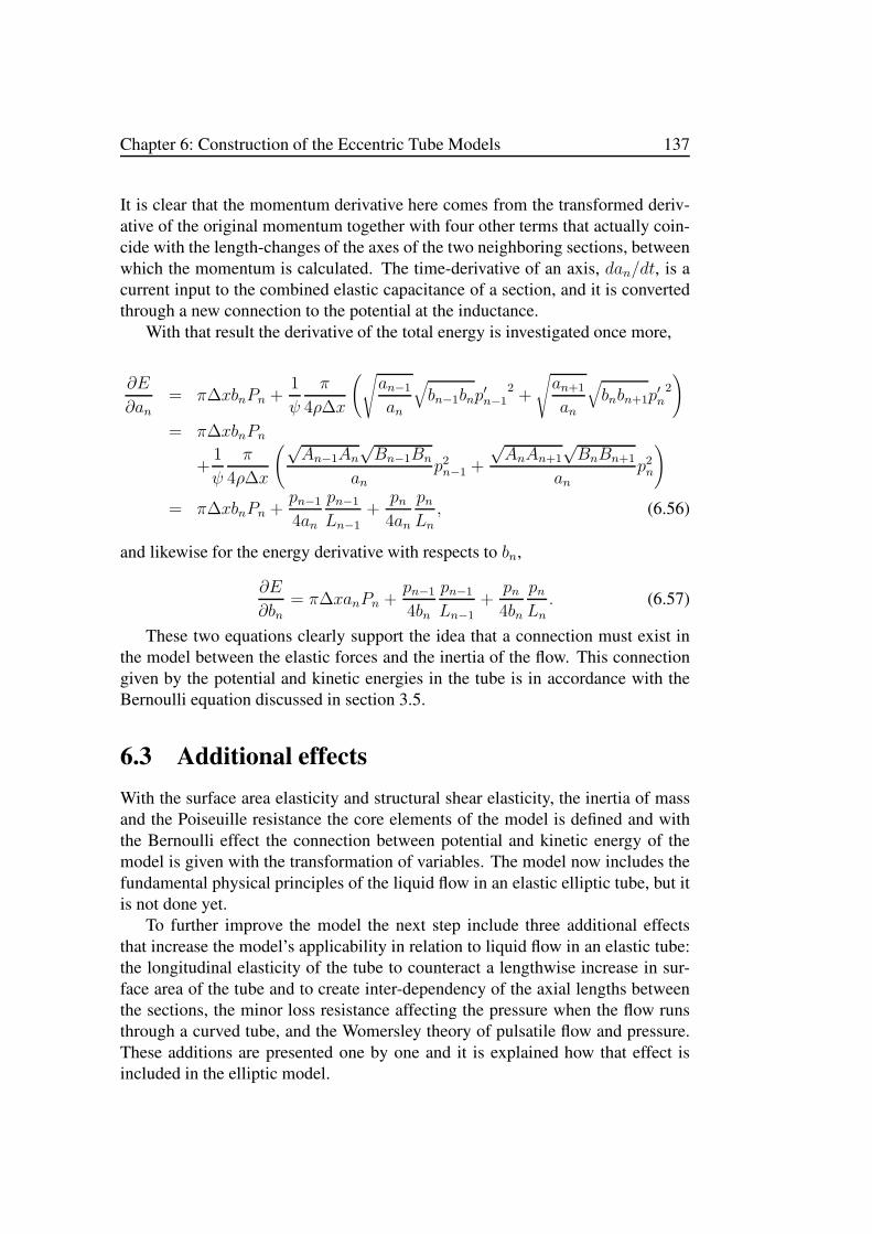
Chapter 6: Construction of the Eccentric Tube Models 137
It is clear that the momentum derivative here comes from the transformed deriv-ative of the original momentum together with four other terms that actually coin-cide with the length-changes of the axes of the two neighboring sections, betweenwhich the momentum is calculated. The time-derivative of an axis, dan/dt, is acurrent input to the combined elastic capacitance of a section, and it is convertedthrough a new connection to the potential at the inductance.
With that result the derivative of the total energy is investigated once more,
∂E
∂an= π∆xbnPn +
1
ψ
π
4ρ∆x
(√an−1
an
√bn−1bnp
′n−1
2+
√an+1
an
√bnbn+1p
′n2
)
= π∆xbnPn
+1
ψ
π
4ρ∆x
(√An−1An
√Bn−1Bn
anp2n−1 +
√AnAn+1
√BnBn+1
anp2n
)
= π∆xbnPn +pn−1
4an
pn−1
Ln−1
+pn4an
pnLn, (6.56)
and likewise for the energy derivative with respects to bn,
∂E
∂bn= π∆xanPn +
pn−1
4bn
pn−1
Ln−1+
pn4bn
pnLn. (6.57)
These two equations clearly support the idea that a connection must exist inthe model between the elastic forces and the inertia of the flow. This connectiongiven by the potential and kinetic energies in the tube is in accordance with theBernoulli equation discussed in section 3.5.
6.3 Additional effects
With the surface area elasticity and structural shear elasticity, the inertia of massand the Poiseuille resistance the core elements of the model is defined and withthe Bernoulli effect the connection between potential and kinetic energy of themodel is given with the transformation of variables. The model now includes thefundamental physical principles of the liquid flow in an elastic elliptic tube, but itis not done yet.
To further improve the model the next step include three additional effectsthat increase the model’s applicability in relation to liquid flow in an elastic tube:the longitudinal elasticity of the tube to counteract a lengthwise increase in sur-face area of the tube and to create inter-dependency of the axial lengths betweenthe sections, the minor loss resistance affecting the pressure when the flow runsthrough a curved tube, and the Womersley theory of pulsatile flow and pressure.These additions are presented one by one and it is explained how that effect isincluded in the elliptic model.
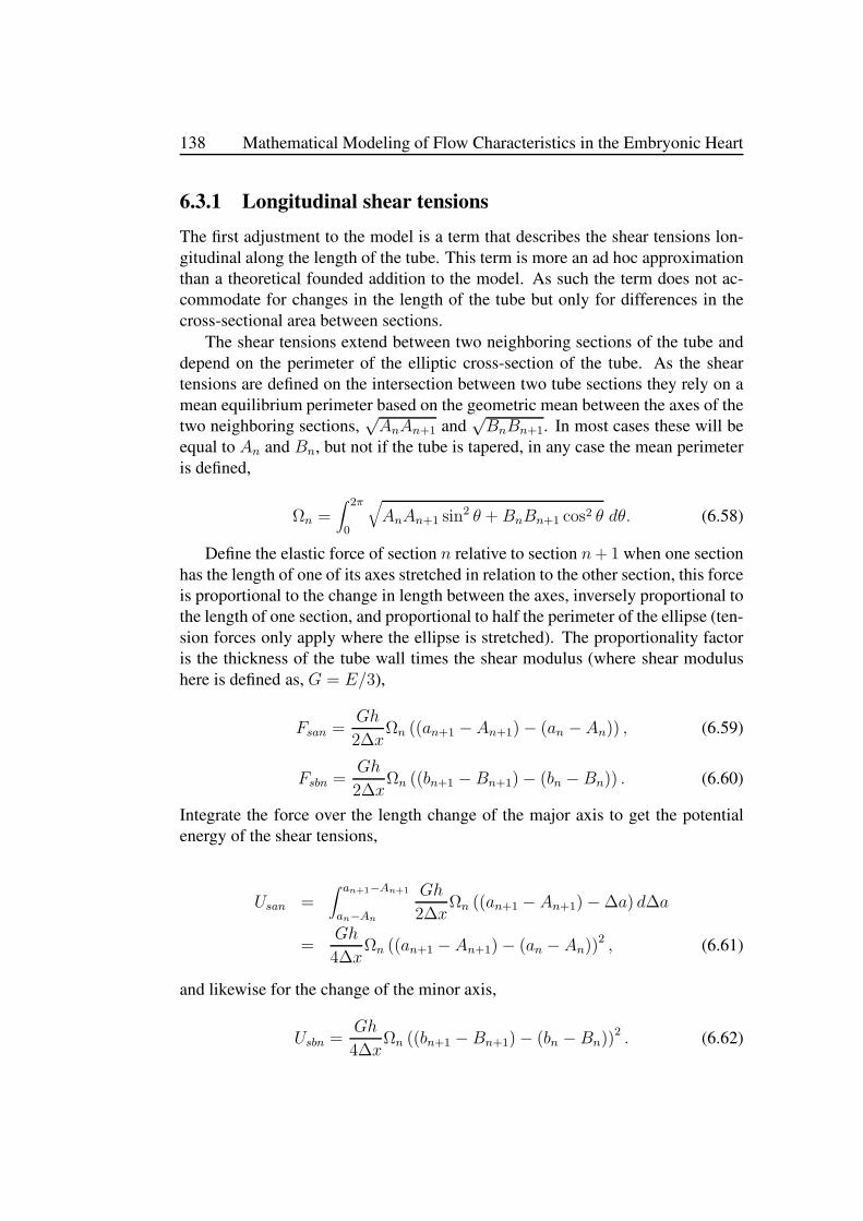
138 Mathematical Modeling of Flow Characteristics in the Embryonic Heart
6.3.1 Longitudinal shear tensions
The first adjustment to the model is a term that describes the shear tensions lon-gitudinal along the length of the tube. This term is more an ad hoc approximationthan a theoretical founded addition to the model. As such the term does not ac-commodate for changes in the length of the tube but only for differences in thecross-sectional area between sections.
The shear tensions extend between two neighboring sections of the tube anddepend on the perimeter of the elliptic cross-section of the tube. As the sheartensions are defined on the intersection between two tube sections they rely on amean equilibrium perimeter based on the geometric mean between the axes of thetwo neighboring sections,
√AnAn+1 and
√BnBn+1. In most cases these will be
equal to An and Bn, but not if the tube is tapered, in any case the mean perimeteris defined,
Ωn =∫ 2π
0
√AnAn+1 sin
2 θ +BnBn+1 cos2 θ dθ. (6.58)
Define the elastic force of section n relative to section n+1 when one sectionhas the length of one of its axes stretched in relation to the other section, this forceis proportional to the change in length between the axes, inversely proportional tothe length of one section, and proportional to half the perimeter of the ellipse (ten-sion forces only apply where the ellipse is stretched). The proportionality factoris the thickness of the tube wall times the shear modulus (where shear modulushere is defined as, G = E/3),
Fsan =Gh
2∆xΩn ((an+1 −An+1)− (an −An)) , (6.59)
Fsbn =Gh
2∆xΩn ((bn+1 − Bn+1)− (bn − Bn)) . (6.60)
Integrate the force over the length change of the major axis to get the potentialenergy of the shear tensions,
Usan =∫ an+1−An+1
an−An
Gh
2∆xΩn ((an+1 − An+1)−∆a) d∆a
=Gh
4∆xΩn ((an+1 − An+1)− (an − An))
2 , (6.61)
and likewise for the change of the minor axis,
Usbn =Gh
4∆xΩn ((bn+1 − Bn+1)− (bn − Bn))
2 . (6.62)

Chapter 6: Construction of the Eccentric Tube Models 139
Use the definition of potential energy of a capacitor to find the capacitance of theshear elasticity, Usan = 1
2(∆an+1 −∆an)
2 /Csan,
Csn = Csan = Csbn =∆x
Gh
2
Ωn. (6.63)
Furthermore these shear tensions should be damped so that there is a smallenergy loss from friction in the tube wall given by the changes in cross-sectionalarea. This is modeled by a resistance in series with the capacitance, the value ofthis resistance is decided from the relation of the characteristic period of an RC-circuit, T = ZsCs, such that all oscillations with frequencies above 100 Hz are bedamped,
Zsn =T
Csn=
0.01 s
Csn. (6.64)
6.3.2 Curvature of the tube
The second addition to the model is the resistance induced by the curvature of thetube, which cause a pressure loss proportional to the product of flow and momen-tum of the flow.
The curvature resistance is a representative of the so called minor losses, whichcover a range of special conditions that produce resistance and energy loss in theliquid flow, dependent on the external conditions presented by the tube. Some ofthe typical minor losses are bends, branches and valves in the tubes, but it is clearthat for the elliptic tube another condition could be relevant, namely the twistingof the tube. That condition is not included in the model, and so it is implicitlyassumed that the tube does not twist or that twisting produce a minor loss, whichis small enough to be ignored.
When the tube curves many interesting things happen for the flow, if the flowhas too high Reynolds number the curve may induce turbulence in the flow, eventhough the flow in straight tubes may be laminar, the curve introduces secondaryflow in the tube, which makes the liquid rotate in the tube, but the most interestingeffect in this case is the resistance introduced by the tube curvature. This resis-tance is caused by increased friction in the tube and it is generally dependent ononly two things, the curvature of the tube and the angle of the bend.
The friction of af bent tube is defined as a loss of pressure in relation to theflow velocity given by Darcy’s equation,
∆P = f∆x
2R
ρv2
2, (6.65)
which is defined for a cylindric tube, given by the radius, R.

140 Mathematical Modeling of Flow Characteristics in the Embryonic Heart
To find how a bend on a tube with elliptic cross-section effects pressure lossin the tube Darcy’s equation is changed to fit an elliptic regime. The length of thetube, ∆x, the flow velocity, v, and the friction factor, f , is defined as usual, butthe radius of the tube is changed to fit with the axes of the ellipse.
The radius, R, in Darcy’s equation is by definition the region of change de-fined in the expression of the Reynolds number, equation 3.4, and it refers to acharacteristic region in which a change of flow can occur, incidentally it is equalto the radius in the cylindric tube but in the elliptic tube it will be more compli-cated. The characteristic length, lc, is given as an intermediate value between Aand B, the axes of the ellipse, defined by the relation,
lc =AB√A2+B2
2
. (6.66)
Thus the elliptic Darcy’s equation becomes,
∆P = fρ∆x
4
√A2 +B2
2A2B2v2. (6.67)
By insertion of the friction factor, f = 32/Re, for steady laminar flow the Poiseuilleequation is achieved (remember that the flow is defined as Q = πAB · v in theelliptic tube),
∆P =32η
ρv
√A2 +B2
2A2B2
ρ∆x
4
√A2 +B2
2A2B2v2 =
4η∆x
π
A2 +B2
A3B3Q, (6.68)
thus proving that the characteristic length defined in equation 6.66 fits in thescheme of Darcy’s equation.
The friction of the bend of the elliptic tube is found through the elliptic ana-logue to equation 4.30,
∆P = (fL + fB)ρ∆x
4
√A2 +B2
2A2B2v2, (6.69)
where fL is the friction factor for the length of the tube defined fL = 32/Re andfB is the friction factor of a bend of the tube defined analogously to equation 4.31,
fB = ξ(θ) ·KB(RB/2lc) · fT (2lc), (6.70)
where fT (2lc) is the friction coefficient for completely turbulent flow, which isthe base that all minor loss coefficients are calculated from, even if the flow in thespecific case is not turbulent,KB(RB/2lc) is a friction factor for a bend of exactly90, dependent on the radius of curvature, RB , relative to the characteristic length,and ξ(θ) is an angular factor for bend angles less than 90.

Chapter 6: Construction of the Eccentric Tube Models 141
In the typical case of a cylindrical tube fT and KB are dependent on the di-ameter of the tube, and it can be argued that the length lc should not be usedfor determination of the numeric values of the functions in equation 6.70 insteadof diameter, but in fact these functions are themselves approximations relativeto a length that appears to be the characteristic length of the Reynolds number.A more elegant approach would be if it were possible to dissolve the bend into‘bend composites’ relative to the directions of the major and minor axes of theelliptic cross-section, but the data from Crane Co. [1982] does not support suchan approach.
The pressure loss in the elliptic bend will be given by the sum,
∆P =4η∆x
π
A2 +B2
A3B3Q + ξKBfT
ρ∆x
4π2
√A2 +B2
2
1
A3B3Q2, (6.71)
where fT is the friction coefficient for completely turbulent flow defined in equa-tion 4.32, KB is defined as a function of the radius of curvature, RB , by equation4.33, and ξ(θ) is defined by equation 4.34.
In terms of resistance to the flow in the energy bond model, the Poiseuilleresistance is already defined, but the resistance of the bend, ZB, becomes,
ZBn =∆PnQn
= ξKBfTρ∆xQn
4√2π2
√anan+1 + bnbn+1
√anan+1
3√bnbn+13 , (6.72)
and with the definition of the momentum of the flow,
pn =
√√√√√anan+1
√bnbn+1√
AnAn+1
√BnBn+1
ψρ∆x
π√anan+1
√bnbn+1
Qn, (6.73)
the flow is eliminated from the equation to give the final resistance of the bendusable in the energy bond model (where the numerical value of the momentum isused because impedance should cause a loss of energy independent of the direc-tion of flow),
ZBn =∆PnQn
=ξKBfTψ
1
4π
√√√√√AnAn+1
√BnBn+1
√anan+1
5√bnbn+15
√anan+1 + bnbn+1
2|pn|.
(6.74)Equation 6.74 defines the friction of the bend of the elliptic tube as a relation
between pressure loss to volume flow. This impedance may be an approximationfrom the data from Crane Co. [1982] for cylindric tubes, but interestingly it isproportional to the momentum of the flow, which means that the impedance growswhen the flow is accelerated. This is very interesting in relation to the pulsatingflow and pressure in the embryonic heart.
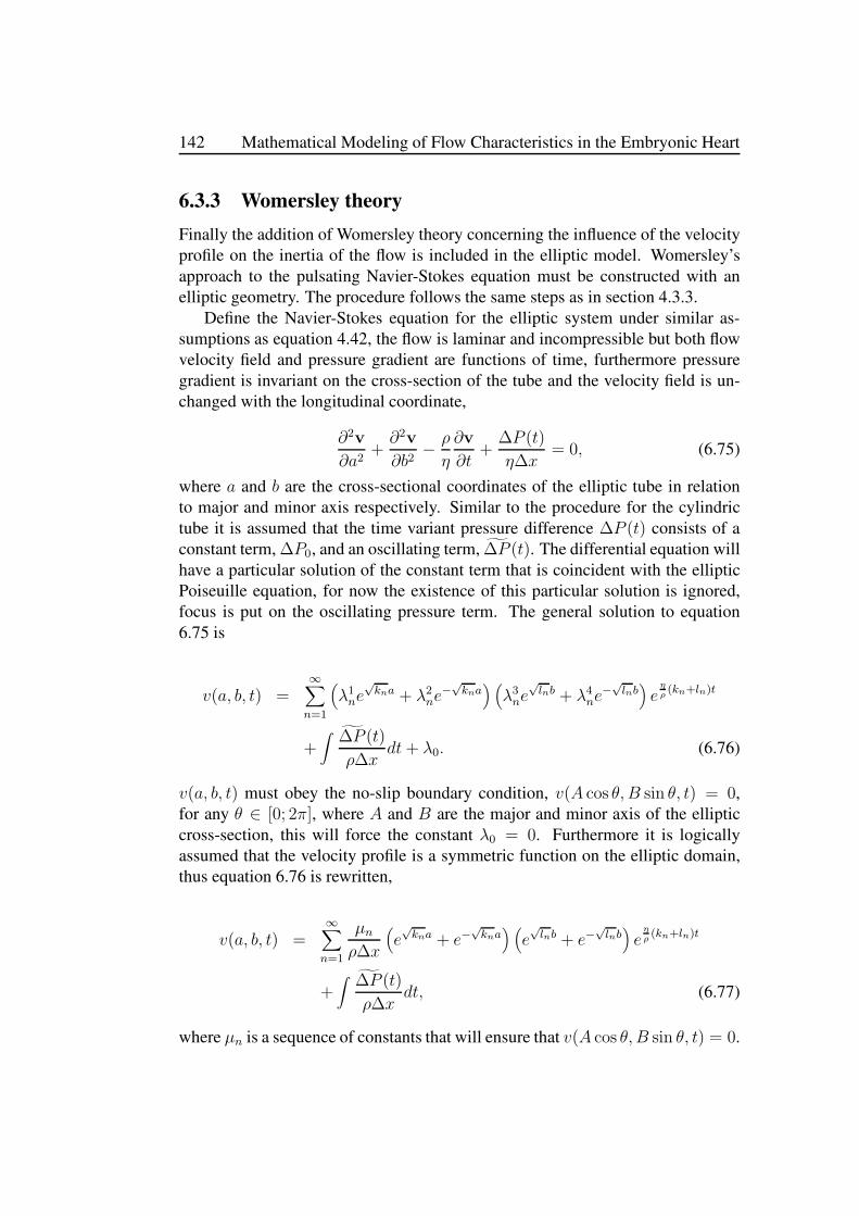
142 Mathematical Modeling of Flow Characteristics in the Embryonic Heart
6.3.3 Womersley theory
Finally the addition of Womersley theory concerning the influence of the velocityprofile on the inertia of the flow is included in the elliptic model. Womersley’sapproach to the pulsating Navier-Stokes equation must be constructed with anelliptic geometry. The procedure follows the same steps as in section 4.3.3.
Define the Navier-Stokes equation for the elliptic system under similar as-sumptions as equation 4.42, the flow is laminar and incompressible but both flowvelocity field and pressure gradient are functions of time, furthermore pressuregradient is invariant on the cross-section of the tube and the velocity field is un-changed with the longitudinal coordinate,
∂2v
∂a2+∂2v
∂b2− ρ
η
∂v
∂t+
∆P (t)
η∆x= 0, (6.75)
where a and b are the cross-sectional coordinates of the elliptic tube in relationto major and minor axis respectively. Similar to the procedure for the cylindrictube it is assumed that the time variant pressure difference ∆P (t) consists of aconstant term, ∆P0, and an oscillating term, ∆P (t). The differential equation willhave a particular solution of the constant term that is coincident with the ellipticPoiseuille equation, for now the existence of this particular solution is ignored,focus is put on the oscillating pressure term. The general solution to equation6.75 is
v(a, b, t) =∞∑
n=1
(λ1ne
√kna + λ2ne
−√kna) (λ3ne
√lnb + λ4ne
−√lnb)e
ηρ(kn+ln)t
+∫
∆P (t)
ρ∆xdt+ λ0. (6.76)
v(a, b, t) must obey the no-slip boundary condition, v(A cos θ, B sin θ, t) = 0,for any θ ∈ [0; 2π], where A and B are the major and minor axis of the ellipticcross-section, this will force the constant λ0 = 0. Furthermore it is logicallyassumed that the velocity profile is a symmetric function on the elliptic domain,thus equation 6.76 is rewritten,
v(a, b, t) =∞∑
n=1
µnρ∆x
(e√kna + e−
√kna) (e√lnb + e−
√lnb)e
ηρ(kn+ln)t
+∫
∆P (t)
ρ∆xdt, (6.77)
where µn is a sequence of constants that will ensure that v(A cos θ, B sin θ, t) = 0.

Chapter 6: Construction of the Eccentric Tube Models 143
Notice that it is not possible to find constants such that each term in the sum willbe zero on the boundary, it is the infinite sum that will be zero while each term ofthe sum is different from zero for (a, b) = (A cos θ, B sin θ).
Assume that the pressure difference is an oscillating function with angularfrequency, ω, that can be written as the Fourier series,
∆P (t) =∞∑
n=1
∆Pneinωt. (6.78)
The pressure equation forces a condition on the exponents, kn + ln = inω ρη,
and a suitable solution is found to be,
kn = inωρ
η
B2
A2 +B2and ln = inω
ρ
η
A2
A2 +B2, (6.79)
hence v(a, b, t) becomes,
v(a, b, t) =∞∑
n=1
1
ρ∆x
∆Pninω
[1− µn
e
aA
√inω ρ
ηA2B2
A2+B2 + e− a
A
√inω ρ
ηA2B2
A2+B2
·e
bB
√inω ρ
ηA2B2
A2+B2 + e− b
B
√inω ρ
ηA2B2
A2+B2
]einωt. (6.80)
With the calculation of the flow velocity in the elliptic domain in equation6.80 an elliptic parallel to the Womersley number is suggested; choose the ellipticWomersley number corresponding to the standard Womersley number forA = B,
αe =
√ωρ
η
2A2B2
A2 +B2. (6.81)
Notice further that the inside the two brackets of equation 6.80 contains thehyperbolic cosine function, this will become important when the volume flow iscomputed as the cross-sectional integral of the flow velocity, as the Taylor seriesapproximation to the hyperbolic functions will be employed to solve the integral,
Q(t) = 4∫ A
0
∫ B√
1−a2/A2
0v(a, b, t)dbda
=∞∑
n=1
1
ρ∆x
∆Pninω
einωt[4∫ A
0
∫ B√
1−a2/A2
01 dbda
−4µn
∫ A
0
∫ B√
1−a2/A2
04 cosh
aAαe
√in
2
cosh
b
Bαe
√in
2
dbda
]

144 Mathematical Modeling of Flow Characteristics in the Embryonic Heart
=∞∑
n=1
1
ρ∆x
∆Pninω
einωt[πAB
−4µn4B
αe√
in2
∫ A
0
∞∑
m=0
(aαe
A
√in2
)2m
(2m)!
∞∑
l=0
(√A2−a2αe
A
√in2
)2l+1
(2l + 1)!da
]
=∞∑
n=1
πAB
ρ∆x
∆Pninω
einωt[1− 4µn
∞∑
m=1
(αe√
in2
)2m
2m1
(m+ 1)!m!
]
=∞∑
n=1
πAB
ρ∆x
∆Pninω
[1− 4µn
J1(αe√−in
)
αe√−in
]einωt. (6.82)
Equation 6.82 shows a remarkable resemblance to equation 4.47 for the os-cillating flow in the cylindric tube, in fact when µn is set to µn = 1
4J0(αe
√−in)
it
shows that v(A cos θ, B sin θ, t) = 0. Thus the oscillating flow becomes,
Q(t) =∞∑
n=1
πAB
ρ∆x
∆Pninω
[1− 1
αe√−in
J1(αe√−in
)
J0(αe√−in
)]einωt
=2πA3B3
η∆x(A2 +B2)
∞∑
n=1
∆Pninα2
e
[1− 1
αe√−in
J1(αe√−in
)
J0(αe√−in
)]einωt,
(6.83)
where J0 and J1 are the Bessel functions of the first kind of order zero and one.The bracketed function in equation 6.83 is f(α, n) from equation 4.49 only
with the elliptic Womersley number, αe,
f(αe, n) = 1− 1
αe√−in
J1(αe√−in
)
J0(αe√−in
) . (6.84)
The earlier analysis of the function revealed that for low values of the Womersleynumber f(αe, n) is close to zero for all values of n, and thus the function in thelower line of equation 6.83 is close to 1/8 making the flow dominated by thePoiseuille resistance, and for high values of αe the function f(αe, n) is close to 1for all values of n making the flow dominated by inertia.
For any n the function f(αe, n) behaves in a similar fashion, only the transitionfrom 0 to 1 becomes steeper for higher values of n, thus it is assumed that equation6.83 can be approximated by,
Q(t) ≈ πAB
ρ∆xf(αe, 1)
∞∑
n=1
∆Pninω
einωt
≈ 2πA3B3
η∆x(A2 +B2)
f(αe, 1)
iα2e
∞∑
n=1
∆Pneinωt. (6.85)

Chapter 6: Construction of the Eccentric Tube Models 145
In the equation ∆P (t) =∑∞n=1∆Pne
inωt is the time variant pressure differenceand p(t) =
∑∞n=1
∆Pn
inωeinωt is the momentum of the oscillating flow. Thus,
η∆x(A2 +B2)
2πA3B3(8 + Ψ(αe))Q(t) ≈
η
ρ
A2 +B2
2A2B2iα2
e p(t), (6.86)
where Ψ(αe) is defined Ψ(αe) =iα2
e
f(αe,1)−8. Notice that the right hand side of this
equation is actually equal to ∆P (t) = iωp(t) and thus the equation demonstratesthat the pressure difference is made up of two terms, one Poiseuille term, ∆Pp(t),and one other term, ∆Pψ(t),
η∆x(A2 +B2)
2πA3B3(8 + Ψ(αe))Q(t) ≈ ∆Pp(t) +
η
ρ
A2 +B2
2A2B2iα2
e pψ(t), (6.87)
where pψ(t) is the momentum referring to ∆Pψ(t). The Poiseuille terms on eachside of the equation cancel out and leaves the relation,
η∆x(A2 +B2)
2πA3B3Ψ(αe)Q(t) ≈ η
ρ
A2 +B2
2A2B2iα2
e pψ(t)
ρ∆x
πABψ(αe)Q(t) ≈ pψ(t), (6.88)
where the function ψ(αe) is defined,
ψ(αe) =1
1− 2αe
√−i
J1(αe
√−i)
J0(αe
√−i)
− 8
iα2e
. (6.89)
The function ψ(αe) is the exact same as ψ(α) in equation 4.57 for the cylindrictube. It has real values in the range from 1 for high values of αe to 4/3 for lowvalues of αe and complex values different from zero only in the transition, whichlies in the domain from αe = 1 to αe = 10.
For higher orders of n the same calculations can be made and assuming cross-terms can be ignored a function similar to ψ(αe) can be defined for each n, withvalues in the range from 1 to 4/3. The transition from 1 to 4/3 will only be moresteep for higher values of n.
Thus it may be assumed that the function ψ(αe) for n = 1 is a sufficient ap-proximation so that the complete description of the time variant volume flow maybe described through a Poiseuille term of the pressure difference, where the par-ticular solution that was ignored at first is brought back into the complete solution,together with a momentum term modified by the function ψ(αe),
Q(t) =πA3B3
4η∆x(A2 +B2)∆P (t) +
1
ψ(αe)
πAB
ρ∆xp(t). (6.90)

146 Mathematical Modeling of Flow Characteristics in the Embryonic Heart
Equation 6.90 demonstrates that the solution to a Navier-Stokes equation fortime-oscillating velocity field and pressure gradient ends with a volume flow de-scribed by the Poiseuille equation with addition of a momentum term where theinertia of the liquid has been modified by the function ψ(αe) defined by equation6.89. This result matches the result achieved for the cylindric tube in section 4.3.3and defines the function multiplied to the inductance in section 6.2.2.
Qn QnQn−1 Pn Pn+1 Qn+1
Zn ZBn
√√ana
n+1
√bnb
n+1√AnA
n+1
√BnB
n+1
@
π∆xbn
π∆xan
π∆xbn+1
π∆xan+1
pn4an
pn4a
n+1
pn4bn
pn4b
n+1
Cσn Cσn+1Cγn Cγn+1
Ln
πFan πFan+1
πFbn πFbn+1
an an+1
an an+1
bn bn+1
bn bn+1
pn
an an+1
bn bn+1
Zsan
Csan
Zsbn
Csbn
∂sn∂an
∂sn∂bn
∂sn+1
∂an+1
∂sn+1
∂bn+1
2bna2n+b2
n
2an
a2n+b2
n
2bn+1
a2n+1
+b2n+1
2an+1
a2n+1
+b2n+1
Figure 6.1: The schematic appearance of the elliptic tube model. Notice how thebranches of an and bn are joined through the capacitances Cσn and Cγn.
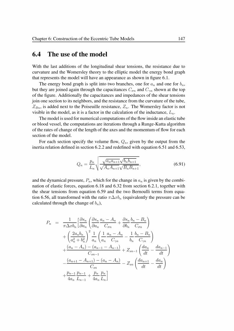
Chapter 6: Construction of the Eccentric Tube Models 147
6.4 The use of the model
With the last additions of the longitudinal shear tensions, the resistance due tocurvature and the Womersley theory to the elliptic model the energy bond graphthat represents the model will have an appearance as shown in figure 6.1.
The energy bond graph is split into two branches, one for an and one for bn,but they are joined again through the capacitances Cσn and Cγn shown at the topof the figure. Additionally the capacitances and impedances of the shear tensionsjoin one section to its neighbors, and the resistance from the curvature of the tube,ZBn, is added next to the Poiseuille resistance, Zn. The Womersley factor is notvisible in the model, as it is a factor in the calculation of the inductance, Ln.
The model is used for numerical computations of the flow inside an elastic tubeor blood vessel, the computations are iterations through a Runge-Kutta algorithmof the rates of change of the length of the axes and the momentum of flow for eachsection of the model.
For each section specify the volume flow, Qn, given by the output from theinertia relation defined in section 6.2.2 and redefined with equation 6.51 and 6.53,
Qn =pnLn
√√√√√anan+1
√bnbn+1√
AnAn+1
√BnBn+1
, (6.91)
and the dynamical pressure, Pn, which for the change in an is given by the combi-nation of elastic forces, equation 6.18 and 6.32 from section 6.2.1, together withthe shear tensions from equation 6.59 and the two Bernoulli terms from equa-tion 6.56, all transformed with the ratio π∆xbn (equivalently the pressure can becalculated through the change of bn),
Pn =1
π∆xbn
[∂sn∂an
(∂sn∂an
an − AnCσn
+∂sn∂bn
bn − Bn
Cσn
)
+
(2anbna2n + b2n
)21
an
(1
an
an − AnCγn
− 1
bn
bn − Bn
Cγn
)
+(an −An)− (an−1 − An−1)
Csn−1+ Zsn−1
(dandt
− dan−1
dt
)
−(an+1 − An+1)− (an − An)
Csn− Zsn
(dan+1
dt− dan
dt
)
+pn−1
4an
pn−1
Ln−1
+pn4an
pnLn
]

148 Mathematical Modeling of Flow Characteristics in the Embryonic Heart
=1
π∆xan
[∂sn∂bn
(∂sn∂an
an − AnCσn
+∂sn∂bn
bn − Bn
Cσn
)
−(
2anbna2n + b2n
)21
bn
(1
an
an −AnCγn
− 1
bn
bn − Bn
Cγn
)
+(bn −Bn)− (bn−1 −Bn−1)
Csn−1
+ Zsn−1
(dbndt
− dbn−1
dt
)
−(bn+1 − Bn+1)− (bn − Bn)
Csn− Zsn
(dbn+1
dt− dbn
dt
)
+pn−1
4bn
pn−1
Ln−1+
pn4bn
pnLn
]. (6.92)
With the definition of volume flow the changes of the length of the axes canbe described with a simple inflow minus outflow relation, but still the resultingvolume change must be divided into changes of the two axes according to therelation given by equation 6.20,
π∆xbndandt
+ π∆xandbndt
= Qn−1 −Qn. (6.93)
To solve this equation use the rule that the pressure is uniform in the energy bondgraph, Pn = Pan = Pbn, which gives a relation between the axial changes,
dandt
= χdbndt, (6.94)
referring to the end of section 6.2.1 χ is given as,
χ =
1bn
∂sn∂an
∂sn∂bn
− 1an
(∂sn∂bn
)2 − 23S2n
(2anbna2n+b
2n
)21
anbn1bn
1an
∂sn∂an
∂sn∂bn
− 1bn
(∂sn∂an
)2 − 23S2n
(2anbna2n+b
2n
)21
anbn1an
, (6.95)
where secondary effects of the longitudinal shear tensions are ignored. Alterna-tively, in some cases the secondary effects may be important as the primary effectswill not show truthful behavior, such as a circular tube with an eccentric deforma-tion, which could be interesting for Liebau’s ring in chapter 5. In those cases χmay be given by,
χ =
[1
Cσn
∂sn∂bn
(1
an
∂sn∂bn
− 1
bn
∂sn∂an
)+
1
Cγn
2
anb2n
(2anbna2n + b2n
)2
+1
Csn−1
1
an
(1− ∂bn−1
∂bn
)1
Csn
1
an
(1− ∂bn+1
∂bn
) ]

Chapter 6: Construction of the Eccentric Tube Models 149
/
[1
Cσn
∂sn∂an
(1
bn
∂sn∂an
− 1
an
∂sn∂bn
)+
1
Cγn
2
a2nbn
(2anbna2n + b2n
)2
+1
Csn−1
1
bn
(1− ∂an−1
∂an
)+
1
Csn
1
bn
(1− ∂an+1
∂an
) ], (6.96)
where the partial derivatives such as ∂an−1
∂anhave to be approximated by functions of
an and an−1. By use of the implicit function theorem if a continuous differentiablefunction f exist on an open space, (an, an−1), such that f(an, an−1) = 0 yet itspartial derivatives are different from zero, then that function defines an−1 as afunction an and through its derivatives,
∂an−1
∂an= −
∂f∂an∂f
∂an−1
. (6.97)
Such a function could be the function f(an, an−1) = e−1
(an−an−1)2 , which for an−1
close to an is close to zero. With the derivatives, ∂f∂an
= 2e−1
(an−an−1)2 (an−an−1)
−3
and ∂f∂an−1
= −2e−1
(an−an−1)2 (an − an−1)
−3, the implicit partial derivative is found,
∂an−1
∂an= − 2e−(an−an−1)−2
(an − an−1)−3
−2e−(an−an−1)−2(an − an−1)−3= 1. (6.98)
Thus for variations between the axes of the different sections the partial deriv-atives may simply be approximated with 1, which will remove the effect of thederivatives in equation 6.96, thus proving that the equation 6.95 is a good approx-imation in the first place. Though to see the effect of the shear elasticity and thusinduce elliptic variations in a cylindric tube in the computations, the partial deriv-atives are instead approximated with ∂an−1
∂an= 1 − δ, where δ is a small number
depending on the sign of an − an−1.The use of secondary effects in the computations heavily increase computation
time, and will not be used except to see necessary eccentric behavior in a non-eccentric tube.
The resulting rate of change for the axes will be as follows,
dandt
=Qn−1 −Qn
π∆x
χ
an + χbn, (6.99)
dbndt
=Qn−1 −Qn
π∆x
1
an + χbn. (6.100)

150 Mathematical Modeling of Flow Characteristics in the Embryonic Heart
Finally the rate of change of the momentum is calculated as the pressure dif-ference minus friction losses from the Poiseuille resistance given by equation 6.48and the resistance due to tube curvature given by equation 6.74 plus the four extraterms from the Bernoulli effect given by equation 6.55,
dpndt
=
√√√√√anan+1
√bnbn+1√
AnAn+1
√BnBn+1
[Pn − Pn+1 −
4
π
η∆x (anan+1 + bnbn+1)√anan+1
3√bnbn+13 Qn
+ξKBfTψ(αe)
1
4π
√√√√√AnAn+1
√BnBn+1
√anan+1
5√bnbn+15
√anan+1 + bnbn+1
2|pn|Qn
]
+pn4an
dandt
+pn
4an+1
dan+1
dt+
pn4bn
dbndt
+pn
4bn+1
dbn+1
dt. (6.101)
The rates of change of the length of the axes and momentum of flow are thethree fundamental equations of the model. If N is the number of sections in themodel the rates of change will constitute a system of 3N non-linear differentialequations, iterated trough a Runge-Kutta algorithm they yield the time-variantfunctions of major and minor axis and for the momentum of flow for all sections,which subsequently can be used to find the time dependent functions of flow andpressure for all sections of the model. This will be the solution to the ellipticmodel.
6.5 The embedded tube model
As an extension to the elliptic tube model another addition is included to make amodel suitable for describing the embryonic heart, as such the elliptic tube modelis changed to the embedded tube model.
At certain stages of the embryonic development the embryonic heart is con-structed in a very ‘simple’ way relative to our normal understanding of a beatingheart, as a length of tube with a muscle that periodically contracts its outer radius.
The construction of the heart tube is layered. The inner layer of the tube iscalled the endocardium it has an almost elliptic cross-section and is very flexible,the outer layer of the tube known as the myocardium has an almost concentriccross-section and is strongly elastic. Between the inner and outer layer of the tubewalls is an easily-deformable elastic gelatinous material known as the cardiacjelly.
The purpose of the cardiac jelly is to convey the muscular contractions ofthe outside myocardium to the inside volume of the tube, in such a way that arelatively small contraction of the outside layer of the tube contracts the insideelliptical cross-section to almost total occlusion.

Chapter 6: Construction of the Eccentric Tube Models 151
The idea in the embedded model is to construct a layered structure consistingof a soft elastic tube of elliptic cross-section embedded inside a stronger elas-tic tube of circular cross-section. In the space between the two tubes an easily-deformable elastic material resides to convey the periodic contractions of the outertube into the inner tube.
This will be an approximation to the embryonic heart as the inner lumen of theheart is only approximately elliptic and the outer perimeter is not entirely circular,in addition when the the outer layer of the embryonic heart contracts it achieves analmost complete closure of the lumen of the inner tube, which will not be possiblein this model.
6.5.1 The tubular cross-section
The layered cross-section of the tube is described through the radius of the outsidelayer, rn, and the major and minor axes of the the inner elliptic layer, an and bn,for each section of the tube. However the inner layer is embedded into the outerconcentric tube in such a way that the major axis of the ellipse is equal to theradius of the outside layer, an = rn.
rn
anbn
Cardiac jelly
Innervolume
Outerlayer
Vjelly = πa2n − πanbn = πan (an − bn)
an = rn
Figure 6.2: The cross-section of the layered tube.
The elastic properties of this complex tube is described with four cross-sectionalcompliances and at least two inter-sectional. The four cross-sectional compliancescome from the elasticity of the concentric outer layer, Crn, the elasticity of theelliptic inner layer, which according to section 6.2.1 must be divided into a com-pliance for the change of the surface area, Cσn, and one for the shear deformationof the elliptic layer, Cγn, and the fourth compliance comes from the elastic prop-erties of the cardiac jelly, Cjn. The inter-sectional compliances are related to theshear stress along the length of the tube and will be described by the longitudinalshear tensions from section 6.3.1.

152 Mathematical Modeling of Flow Characteristics in the Embryonic Heart
6.5.2 Elasticity of the tube wall
Following the procedure in section 6.2.1 the elasticity of the inner and outer layercan be calculated through the potential energy stored by a deformation of the layer.This energy is given by the pressure on the layer integrated over volume change,which is unfortunately not a linear relation.
To make it linear the variables are transformed from volume change to achange in the axes of the inner ellipse, and then the energy is given by the in-tegral of the surface-specific elastic modulus, the surface area, the curvature ofthe surface and the deformation of the axes.
For the outer circular layer this relation is quite simple, since both surfacearea and curvature are simple functions in a circular scheme, thus the increase inenergy will be given as in section 4.2.1,
Urn =∫ π
2
−π2
∫ an
An
∆xEouthoutAn
(a− An) dadθ =π
2
∆xEouthoutAn
(an − An)2 ,
(6.102)where surface-specific elastic modulus is given by the thickness of the outer layer,hout, times Young’s modulus for that type of material, Eout. The equilibriumradius for the tube at rest is An and ∆x is the length of section n of the tube.
Notice that the energy is only integrated over the arc from −π/2 to π/2 incontradiction to how it is done in the cylindric model in section 4.2.1. This is dueto the fact that the effort of the energy bond related to the changes of the majoraxis only covers half of the force related to one section, ern = πFrn, whereas theeffort of the concentric model is equal to the full force on a section, en = 2πFn.
Given the expression for the potential energy of a capacitor, Urn = 12∆a2n/Crn,
this defines the capacitance associated with the length-change of the radius of theouter layer,
Crn =An
π∆xEouthout. (6.103)
The force subjected by this capacitance is simply computed as the change inthe radius of the outer layer divided by the capacitance (and divided by π becauseof the relation of force to effort, ern = πFrn),
Frn =∆xEouthout
An∆an, (6.104)
the interesting part about this force is that it only affects the radius of the outerlayer, that is the major axis of the inner elliptic layer. This is in contrast to all theother forces in the model.

Chapter 6: Construction of the Eccentric Tube Models 153
For the axes of the inner elliptic layer the relation is more complicated becausethe surface area and surface curvature are much more complicated functions, fur-thermore a change of the axes will produce shear forces in the elliptic layer, whichmust also be taken into account.
The process of finding the elastic forces from a deformation of the ellipticlayer is described in section 6.2.1. The end result is a pair of coupled forces,where two forces acts on the major axis of the ellipse,
Fσan =EinhinSn
∂sn∂an
(∂sn∂an
∆an +∂sn∂bn
∆bn
), (6.105)
Fγan = GinhinSn
(2anbna2n + b2n
)21
an
(1
an∆an −
1
bn∆bn
), (6.106)
and two other forces, one proper and one shear, acts on the minor axis,
Fσbn =EinhinSn
∂sn∂bn
(∂sn∂an
∆an +∂sn∂bn
∆bn
), (6.107)
Fγbn = −GinhinSn
(2anbna2n + b2n
)21
bn
(1
an∆an −
1
bn∆bn
), (6.108)
where hin is the thickness of the inner elliptic layer, Ein is Young’s modulus, andGin is the shear modulus for the layer. The surface area of section n of the ellipticlayer is described through the second elliptic integral,
sn = ∆x∫ 2π
0
√a2n sin
2 θ + b2n cos2 θ dθ, (6.109)
where Sn is the corresponding equilibrium surface area, and where ∂sn/∂an and∂sn/∂bn are its derivatives with respect to the axial changes.
The forth elasticity comes from the volume deformation of the elastic mate-rial between the two layers, the cardiac jelly. The volume of the space betweenthe layers is a function of the difference between the volume of the outer layer,∆xπa2n, and the volume of the inner elliptic layer, ∆xπanbn yielding the volumeof the cardiac jelly, Vjn = ∆xπ(a2n − anbn). Thus the volume change will be,
dVjn = ∆xπ ((2an − bn)dan − andbn) . (6.110)
Transform from an to a∗n by applying the transformation relation,
dan =an
2an − bnda∗n, (6.111)
which gives a symmetric expression for the volume change,
dVjn = ∆xπan (da∗n − dbn) . (6.112)

154 Mathematical Modeling of Flow Characteristics in the Embryonic Heart
The increased pressure inside the cardiac jelly is given by the relative volumechange, that is the change in volume compared to the original volume,
dPn = KdVjnVj0
= KdVjn
∆xπ (A2n − AnBn)
, (6.113)
where K is an unspecific elastic modulus of the cardiac jelly. It is clear thatthe elastic modulus involved in this expression will have both proper and shearqualities corresponding to the complicated deformation of the arc-shaped volumeinhabited by the cardiac jelly, in this thesis it is assumed that the elastic modulusused can be approximated by a single constant similar to Youngs modulus, thoughfurther investigation may clarify this question.
Let ∆Pn = Pn − P0 and ∆Vjn = Vjn − Vj0 be the first order approximationsto the infinitesimals of equation 6.113, then integrate the pressure over the volumeincrease from Vj0 to Vjn to get the potential energy,
Ujn =∫
∆PndVjn =∫ Vjn
Vj0
K
∆xπ(A2n −AnBn)
(V − Vj0) dV
=K
2∆xπ (A2n − AnBn)
(Vjn − Vj0)2 . (6.114)
By the expression for the potential energy of a capacitor, Ujn = 12δV 2
jn/Cjn, thecapacitance is defined,
Cjn =∆xπ(A2
n −AnBn)
K. (6.115)
The forces subjected to the layers of the tube by the elasticity of the cardiacjelly is paired similarly to the elastic forces given in section 6.2.1, one for the mi-nor axis of the ellipse and one for the major axis. The forces are found by tracingbackwards through the equations, thus the force on the major axis becomes,
Fjan = −∆xπ(2an − bn)K
A2n −AnBn
((2an − bn)∆an − an∆bn) , (6.116)
and the force on the minor axis,
Fjbn = ∆xπanK
A2n −AnBn
((2an − bn)∆an − an∆bn) . (6.117)
Thereby all four cross-sectional elastic properties have been described, butnotice how the first did only produce one force on the outside layer whereas theother three produced paired forces on the major and minor axis respectively.

Chapter 6: Construction of the Eccentric Tube Models 155
The intersectional elasticity is given by the longitudinal shear tensions de-scribed in section 6.3.1. The first, Csan, is made from a combination of the elas-ticity of the outer layer and the elasticity of the elliptic inner layer and thus alsorefers to section 4.3.1,
Csan =2∆x
4πGouthout√AnAn+1 +GinhinΩn
, (6.118)
and the second, Csbn, comes alone from the elasticity of the inner layer,
Csbn =2∆x
GinhinΩn, (6.119)
where Ωn is the geometric mean surface area between two neighboring tube sec-tions defined by equation 6.58 and Gin and Gout are the shear modulus of the walllayers, equal to one third of Young’s modulus.
As described in section 6.3.1 the longitudinal shear tensions are accompaniedby a damping resistance, Zsan = T/Csan and Zsbn = T/Csbn, where T = 0.01s is the characteristic time of the RC-circuit made up by the capacitance and im-pedance in serial coupling in the energy bond graph.
6.5.3 The use of the model
With the description of the four cross-sectional elastic capacitances and the lon-gitudinal shear tensions the total elastic properties of the tube is described. Inaddition the embedded model is equipped with an inductance representing theinertia, Ln, with the Womersley inertia correction factor, ψ(αe), a Poiseuille re-sistance, Zn, and a resistance due to curvature of the tube, ZBn. The energy bondgraph of this complicated model is shown in figure 6.3.
The model is used for numerical computations of the flow inside an com-plicated elastic tube or in the embryonic heart, the computations are iterationsthrough a Runge-Kutta algorithm of the derivatives of the length of the axes andthe momentum for each section of the model.
For each section specify the volume flow, Qn,
Qn =pnLn
√√√√√anan+1
√bnbn+1√
AnAn+1
√BnBn+1
, (6.120)
and the dynamical pressure, Pn,

156 Mathematical Modeling of Flow Characteristics in the Embryonic Heart
Qn QnQn−1 Pn Pn+1 Qn+1
Zn ZBn
√√
anan+1
√bnb
n+1√AnA
n+1
√BnB
n+1
@
π∆xbn
π∆xan
π∆xbn+1
π∆xan+1
pn4an
pn4a
n+1
pn4bn
pn4b
n+1
Cσn Cσn+1Cγn Cγn+1
Ln
πFan πFan+1
πFbn πFbn+1
an
an an+1
bn bn+1
bn bn+1
pn
an an+1
bn bn+1
Zsan
Csan
Zsbn
Csbn
∂sn∂an
∂sn∂bn
∂sn+1
∂an+1
∂sn+1
∂bn+1
2bna2n+b2
n
2an
a2n+b2
n
2bn+1
a2n+1
+b2n+1
2an+1
a2n+1
+b2n+1
Cjn Cjn+1
an
2an−bn
an+1
2an+1−a
n+1@
1an
1an+1
Crn Crn+1
a∗n a∗n+1
Figure 6.3: The schematic appearance of the embedded tube model. The branchesof an and bn are joined through three energy bonds; one for the surface area spe-cific compliance, Cσn, one for the surface structural shear compliance Cγn andone for the volume specific compliance of the cardiac jelly, Cjn. Additionally thecompliance of the outer myocardial layer is represented through Crn.

Chapter 6: Construction of the Eccentric Tube Models 157
Pn =1
π∆xbn
[an −AnCrn
+∂sn∂an
(∂sn∂an
an − AnCσn
+∂sn∂bn
bn − Bn
Cσn
)
+
(2anbna2n + b2n
)21
an
(1
an
an − AnCγn
− 1
bn
bn −Bn
Cγn
)
−(∆xπ)2(2an − bn)
((2an − bn)
an −AnCjn
− anbn − Bn
Cjn
)
+(an −An)− (an−1 −An−1)
Csn−1+ Zsn−1
(dandt
− dan−1
dt
)
−(an+1 −An+1)− (an − An)
Csn− Zsn
(dan+1
dt− dan
dt
)
+pn−1
4an
pn−1
Ln−1
+pn4an
pnLn
]
=1
π∆xan
[∂sn∂bn
(∂sn∂an
an −AnCσn
+∂sn∂bn
bn −Bn
Cσn
)
−(
2anbna2n + b2n
)21
bn
(1
an
an − AnCγn
− 1
bn
bn − Bn
Cγn
)
+(∆xπ)2an
((2an − bn)
an − AnCjn
− anbn −Bn
Cjn
)
+(bn − Bn)− (bn−1 − Bn−1)
Csn−1
+ Zsn−1
(dbndt
− dbn−1
dt
)
−(bn+1 −Bn+1)− (bn − Bn)
Csn− Zsn
(dbn+1
dt− dbn
dt
)
+pn−1
4bn
pn−1
Ln−1+
pn4bn
pnLn
]. (6.121)
With the definition of volume flow the changes of the volume per section canbe described with a simple inflow minus outflow relation,
π∆xbndandt
+ π∆xandbndt
= Qn−1 −Qn. (6.122)
Unfortunately the axial changes can not be derived from this equation alone, afurther condition of the pressure is needed. In the model the pressure can bedescribed through two ways as demonstrated in equation 6.121, which gives arelation between the axial changes, dan
dt= χdbn
dt, with χ given by,

158 Mathematical Modeling of Flow Characteristics in the Embryonic Heart
χ =
12
(bnan
(∂sn∂bn
)2 − ∂sn∂an
∂sn∂bn
)+ S2
n
3
(2anbna2n+b
2n
)21
anbn+ π∆xKSn
Einhin
a2nA2
n−AnBn
12
((∂sn∂an
)2 − bnan
∂sn∂an
∂sn∂bn
)+ S2
n
3
(2bn
a2n+b2n
)2+ π∆xKSn
Einhin
an(2an−bn)A2
n−AnBn+ π∆xEouthoutSn
2EinhinAn
,
(6.123)which gives the resulting rate of change for the axes,
dandt
=Qn−1 −Qn
π∆x
χ
an + χbn, (6.124)
dbndt
=Qn−1 −Qn
π∆x
1
an + χbn. (6.125)
Notice that in section 6.4 another more complicated procedure for calculating χwas introduced for the cases where the simple approach would not suffice, butgiven the already eccentric construction of the embedded model with an asym-metric distribution of the cardiac jelly that procedure will not be necessary here.
The rate of change of the momentum is calculated as the pressure differenceminus friction loss plus the contributions from the Bernoulli coupling,
dpndt
=
√√√√√anan+1
√bnbn+1√
AnAn+1
√BnBn+1
[Pn − Pn+1 −
4
π
η∆x (anan+1 + bnbn+1)√anan+1
3√bnbn+13 Qn
−ξKBfTψ(αe)
1
4π
√√√√√AnAn+1
√BnBn+1
√anan+1
5√bnbn+15
√anan+1 + bnbn+1
2|pn|Qn
]
+pn4an
dandt
+pn
4an+1
dan+1
dt+
pn4bn
dbndt
+pn
4bn+1
dbn+1
dt. (6.126)
The three derivatives, dandt
, dbndt
and dpndt
constitute a system of 3N non-lineardifferential equations, where N is the number of sections in the model. A solutionto this system of differential equations is found numerically using a Runge-Kuttaalgorithm, which yields the time-dependent functions of the axes and momentumfor each section of the model, subsequently the functions of flow and pressureis found through the use of equation 6.120 and 6.121. The set of all five time-dependent functions of the axial lengths, momentum of flow, pressure and volumeflow is a complete solution to the embedded model.

Chapter 7
The Embryonic Heart Model
As specified in chapter 2 the embryonic heart is formed as a simple straight elastictube that gradually twists and turns during the Hamburger and Hamilton develop-ment stages (HH-stages) 10 to 24. During this process known as cardiac loopingthe heart starts beating at HH-stage 10 and from the different looping proceduresand overall growth of the embryo the liquid flow will experience great changesin heart rate, stroke volume, tubular dimensions and physical parameters (amongother things) during the following HH-stages.
It was argued in section 2.2 that the interesting stages of the tubular heart areHH-stage 10 with the onset of cardiac looping and the beating of the heart, HH-stage 12 when the looping heart has formed in the shape of a ‘c’ and a stable flowrate is observed, HH-stage 14 when the looping heart has formed in the shape ofan ‘s’ and the primitive atrium is fully developed, and HH-stage 16 with a fullys-shaped heart that includes all the cardiac segments of the looping heart. Theseare the four stages of the tubular that will be the focus of this chapter.
In the following a model for the embryonic heart tube will be setup followingthe four steps introduced in section 5.2, though here it will make more sense toinclude them in a different order: First a tracing of the heart tube, then boundaryconditions, parameter estimation, and finally the pumping mechanism.
7.1 Tracing of the embryonic heart
Acquisition of accurate numbers for the dimensions of the heart tube is unfortu-nately a problem for embryological research, in vivo imaging techniques are stillat a very early stage of development and the embryonic heart so small that onlyapproximal data is available - and usually in the form of images rather than numer-ical values. So far the acquisition of dimensional data has not been the focus ofembryological research although it is of great importance for the understanding of
159

160 Mathematical Modeling of Flow Characteristics in the Embryonic Heart
the pumping function of the tubular embryonic heart, due to its small dimensionsthe circulatory system of the embryo has just been regarded as a vascular systemthat shows flow at low Reynolds numbers.
In order to make a tracing of the embryonic heart loop the following values areneeded: length of each of the cardiac segments (left and right ventricle, primitiveatrium, outflow tract etc.), end-diastole diameter at defining points along the hearttube preferably a few measurements for each cardiac segment, measurements ofend-diastole inner lumen of the heart tube or a measurement of the percentage thatcardiac jelly take of the cross-sectional area of the heart tube (for each of the car-diac segments), thickness of the outer myocardial layer and the inner endocardiallayer, and curvature of the heart, which is not necessarily uniform.
The paper by Männer [2000] includes a number of very nice in ovo (in the egg)images of embryonic hearts in the relevant stages of development using scanningelectron microscopy, see figure 2.1, from which it is possible to estimate approx-imal external lengths and diameters (assuming that width in the images can betranslated directly to diameter in the model) of the observed cardiac segments, thedata is presented in table 7.1.
In addition to the data presented in table 7.1 it is possible to estimate an ap-proximate radius of curvature for the looping heart at the beginning of dextrallooping (HH-stage 10) from Männer [2000] fig. 1.D. The heart appears to have analmost uniform radius of curvature, RB = 550 µm, from the venous pole to theoutflow tract. Due to the complicated three dimensional looping at later stages itwas not possible to make similar estimates for HH-stage 12, 14 or 16.
Additionally some dimensional data can be found in various papers from ex-perimental embryological research, below table 7.2 to 7.5 list some dimensionalmeasurements and model estimations found in the embryological literature. Thecombined tracing of the looping heart with dimensional data from table table 7.1and tables 7.2 to 7.5 is shown on figures 7.1 to 7.4, which include the sketches ofthe embryonic heart at the appropriate stages.
The disagreement of the reported dimensional values is notable, for instancetable 7.5 lists five different measurements of the outside dimension of the HH-stage 16 ventricle, which under the simple assumption of a circular cross sectiongives the following diameters for the ventricle 240 µm, 250 µm, 256 µm, 542 µm,and 800 µm, especially the measurements of outside perimeter and cross-sectionalarea from table 7.3, 7.4 and 7.5 seem to suggest diameters twice the size of othercorresponding numbers.
For HH-stage 16 a much larger set of dimensional information is needed tocomplete the model with all the cardiac segments present compared to the otherstages, and even though this stage is the most researched of the four some num-bers are still missing, most importantly the thickness of the myocardial layer andthe radius of curvature for the heart tube. Both are possible to estimate fromknowledge of the surrounding stages.

Chapter 7: The Embryonic Heart Model 161
Stages HH-10 HH-12 HH-14 HH-16*LengthsSinus venosis 50 µm** 70 µm 170 µm 230 µmPrimitive atrium 200 µm 230 µm 470 µmLeft ventricle 130 µm 270 µm 480 µm 700 µmRight ventricle 250 µm 370 µm 500 µm 500 µmProximal outflow tract*** 230 µm 250 µm 230 µm 270 µmDistal outflow tract*** 100 µm 170 µmDiametersLeft vein 150 µm 130 µm 250 µm 200 µmRight vein 100 µm 130 µm 250 µm 200 µmSinus venosis 330 µm** 350 µm 450 µm 470 µmVenous pole 300 µm 330 µm 250 µm 370 µmCentral atrium 320 µm 270 µm 370 µmUpper atrium 280 µm 270 µm 350 µmAtrioventricular canal 250 µm 330 µmLower left ventricle 250 µm 280 µm 380 µmCentral left ventricle 270 µm 250 µm 350 µm 470 µmUpper left ventricle 330 µm 400 µmLeft lateral furrow 250 µm 250 µm 320 µm 350 µmLower right ventricle 330 µm 350 µmCentral right ventricle 250 µm 230 µm 320 µm 350 µmUpper right ventricle 170 µm 250 µm 300 µmConoventricular sulcus 200 µm 150 µm 200 µm 270 µmProximal outflow tract*** 170 µm 150 µm 200 µm 250 µmDistal outflow tract*** 150 µm 180 µm 200 µmArterial outlet 120 µm 130 µm 130 µm 170 µm
Table 7.1: Estimated external dimensions of the early stages of the looping em-bryonic heart based on images from Männer [2000] fig. 1.D (HH-stage 10), fig.1.G (HH-stage 12), fig. 3.A and 3.A´ (HH-stage 14), fig. 3.C, 3.C´, 4.A, 4.A´ and4.A´´ (HH-stage 16). (*) Notice that at HH-stage 16 the looping heart makes itdifficult to estimate some dimensions due to perspective in the images. (**) AtHH-stage 10 the heart has not yet developed the sinus venosis of the later stages,here it is merely used to describe the inflow portion of the heart tube. (***) In car-diac morphology research it is debated at what stages the conus and truncus partof the outflow tract is formed [Martinsen, 2005], therefore the proximal and distaloutflow tract are not meant as reference to those specific cardiac segments, theyrefer only to the dimensions of the outflow tract present at the particular stage.

162 Mathematical Modeling of Flow Characteristics in the Embryonic Heart
Primitive atriumor venous sinusLength: 50 µmDiameter: 330 µm
aaaa
aaaa
aLeft veinDiameter: 150 µm
Left ventricleLength: 130 µm
((((((((((
Radius of curvatureRB = 550 µm
aaaa
aaaa
aaa
,,,,,,,,,
Right ventricleLength: 250 µm
Proximal outflow tractLength: 230 µm
Right veinDiameter: 100 µm
Venous poleDiameter: 300 µm
Left ventricleDiameter: 270 µm
Left lateral furrowDiameter: 250 µm
Right ventricleDiameter: 250 µmLumen: 70 µmMyocardium: 18 µmCardiac jelly: 52 µm
`````````
Conoventricular sulcusDiameter: 200 µm
hhhhhhhh
Proximal outflow tractDiameter: 170 µm
Arterial outletDiameter: 120 µm
Figure 7.1: A sketch of the HH-stage 10 embryonic heart with all the found di-mensional values noted on the figure.
HH-stage 10 Dimension ReferenceLength of the heart tube 500 µm [Latacha et al., 2005]Length of the heart tube 700 µm [Taber, 2006b]External diameter of the ventricle 200 µm [Latacha et al., 2005]External diameter of the ventricle 200 µm [Taber, 2006b]Lumen diameter of the ventricle 70 µm [Latacha et al., 2005]Thickness of the myocardial layer 18 µm [Latacha et al., 2005]Thickness of the myocardial layer 18 µm [Taber, 2006b]Thickness of the cardiac jelly 47 µm [Latacha et al., 2005]Thickness of the cardiac jelly 56 µm [Taber, 2006b]
Table 7.2: Reports of HH-stage 10 embryonic heart dimensions. In addition Taber[1998] reports that the thickness of the myocardial layer is two cells thick whereasthe thickness of the endocardial layer is one cell thick. Notice however that allthree articles assumes a more or less concentric position of the cardiac jelly andinner lumen of the heart tube.

Chapter 7: The Embryonic Heart Model 163
Left veinDiameter: 130 µm
@@@
Venous sinusLength: 70 µmDiameter: 350 µm
(((((((((
Primitive atriumLength: 200 µm
Left ventricleLength: 270 µm
((((((((((((((
Radius of curvatureRB = 500 µm
QQQQQQQQQQQ
Right ventricleLength: 370 µm
((((((((((((((((((
Proximal outflow tractLength: 250 µm
Right veinDiameter: 130 µm
Venous poleDiameter: 330 µm
Central atriumDiameter: 320 µm
((((((((
((((((
Upper atriumDiameter: 280 µm
((((((((
(((((Lower left ventricle
Diameter: 250 µm((((
((((((Central left ventricle
Diameter: 250 µm((((
(((Left lateral furrowDiameter: 250 µm
Central right ventricleDiameter: 230 µmMyocardium: 15 µmCardiac jelly: 70 µm
Upper right ventricleDiameter: 170 µm
Conoventricular sulcusDiameter: 200 µm
hhhhhhhh
Proximal outflow tractDiameter: 150 µm
Distal outflow tractDiameter: 150 µm
Arterial outletDiameter: 130 µm
Dorsal aortaDiameter: 110 µm
Figure 7.2: A sketch of the HH-stage 12 embryonic heart with all the found di-mensional values noted on the figure. Notice the thickness of the cardiac jelly,Zamir et al. [2003] estimate the thickness to around 90 % of the tube radius butfrom images by Männer et al. [2008] the thickness seems to be closer to 50 %.
HH-stage 12 Dimension ReferenceOuter radius of the heart tube 150 µm [Zamir et al., 2003]Outside perimeter of the ventricle 1800±30 µm [Keller et al., 1990]Cross-sectional area of the ventricle 0.23±0.01 mm2 [Keller et al., 1990]Outer diameter of the outflow tract 290±10 µm [Keller et al., 1990]Diameter, atrioventricular canal 500 µm [Hu et al., 1991]Cross-sectional area of the aorta 0.01±0.002 mm2 [Hu and Clark, 1989]Inner radius of the heart tube 25 µm [Zamir et al., 2003]Thickness of the myocardial layer 15 µm [Zamir et al., 2003]Thickness of the cardiac jelly 135 µm [Zamir et al., 2003]Radius of curvature, heart tube 500 µm [Zamir et al., 2003]
Table 7.3: Reports of HH-stage 12 embryonic heart dimensions. In addition thestatement from Taber [1998] that the myocardial layer is two cells thick and theendocardial layer only one still holds for HH-stage 12, while Hu and Clark [1989]report the myocardium to be around 3-5 cells thick and the endocardium 1.

164 Mathematical Modeling of Flow Characteristics in the Embryonic Heart
Left veinDiameter: 250 µm
@@
Venous sinusLength: 170 µm
XXXXXX
Central Primitive atriumLength: 230 µmDiameter: 270 µm
Upper primitive atriumDiameter: 270 µm
Left ventricleLength: 480 µm
Right ventricleLength: 500 µm
Proximal outflow tractLength: 230 µm
Distal outflow tractLength: 100 µm
Dorsal aortaDiameter: 115 µm
Right veinDiameter: 250 µm
Venous sinusDiameter: 450 µm
Venous poleDiameter: 250 µm
Atrioventricular canalDiameter: 250 µmCardiac jelly: 60 µm
Lower left ventricleDiameter: 280 µm
!!!!!!!!!!
Central left ventricleDiameter: 350 µm
!!!!!!!!
Upper left ventricleDiameter: 330 µm
Left lateral furrowDiameter: 220 µm
Lower right ventricle
Diameter: 330 µm
Central right ventricleDiameter: 320 µmMyocardium: 18 µmCardiac jelly: 85 µm
Upper right ventricleDiameter: 250 µm
Conoventricular sulcusDiameter: 200 µm
PPPPP
Proximal outflow tractDiameter: 200 µm
PPPPPPP
Distal outflow tractDiameter: 180 µm
Arterial outletDiameter: 130 µm
Figure 7.3: A sketch of the HH-stage 14 embryonic heart with all the found di-mensional values noted on the figure. A measure of the radius of curvature ismissing for this stage, therefore an average between HH-stage 12 and HH-stage16 is used, RB = 550 µm.
HH-stage 14 Dimension ReferenceOutside perimeter of the ventricle 2200±80 µm [Keller et al., 1990]Cross-sectional area of the ventricle 0.34±0.03 mm2 [Keller et al., 1990]Outer diameter of the outflow tract 350±10 µm [Keller et al., 1990]Cross-sectional area of the aorta 0.04±0.004 mm2 [Hu and Clark, 1989]Ventricular cardiac jelly thickness* 70-100 µm [Männer et al., 2010]AV-canal cardiac jelly thickness* 40-80 µm [Männer et al., 2010]
Table 7.4: Reports of HH-stage 14 embryonic heart dimensions. For some reasonnumerical data for this stage of development is very scarce. (*) The thickness ofthe cardiac jelly is estimated from fig. 1.B in [Männer et al., 2010]. The statementfrom Taber [1998] that the myocardial layer is two cells thick and the endocardiallayer is one cell thick still holds for HH-stage 14.

Chapter 7: The Embryonic Heart Model 165
Radius of curvaturefrom venous poleto distal outflow tractRB = 600 µm
Left veinDiameter: 200 µm
Venous sinusLength:
230 µmDiameter:
470 µm
Venous poleDiameter:
370 µm
Centralprimitive atriumLength: 470 µmDiameter: 370 µm
Upper primitive atriumDiameter: 350 µm
Atrioventricular canalDiameter: 330 µm
AAAA
Distal outflow tractLength: 170 µmDiameter: 200 µm
Dorsal aortaDiameter: 140 µm
Right veinDiameter: 200 µm
Lower left ventricleDiameter: 380 µm
Central left ventricleLength: 700 µmDiameter: 470 µmMyocardium: 20 µmCardiac jelly: 85 µm
Upper left ventricleDiameter: 400 µm
Left lateral furrowDiameter: 350 µm
Lower right ventricleDiameter: 350 µm
Central right ventricleLength: 500 µmDiameter: 350 µmMyocardium: 20 µmCardiac jelly: 85 µm
Upper right ventricleDiameter: 300 µm
HHHHHH
Conoventricular sulcusDiameter: 270 µm
JJJJ
Proximal outflow tractLength: 270 µmDiameter: 250 µmJ
JJJ
Arterial outletDiameter: 170 µm
Figure 7.4: A sketch of the HH-stage 16 embryonic heart with all the found di-mensional values noted on the figure.
For the thickness of the myocardial layer Taber [1998] reports that the thick-ness of the ventricular wall remains relatively thin with the needs of the my-ocardium being met entirely by diffusion from the lumen until the onset of tra-beculation at HH-stage 17, and furthermore Martinsen [2005] reports that thethickness of the myocardial layer only changes slightly from 1-2 cell layers to3-4 cell layers during the stages from HH-stage 12 to 21, thus it may be assumedthat the thickness of the myocardial layer is almost constant from HH-stage 10 toHH-stage 16.
No records of the radius of curvature for a HH-stage 16 heart tube has beenfound, however Miller et al. [1997a] reports of a finite element model of a HH-stage 18 curved heart tube with a average radius of curvature, RB = 670 µm.

166 Mathematical Modeling of Flow Characteristics in the Embryonic Heart
HH-stage 16 Dimension ReferenceOutside radius of the ventricle 128 µm [Taber et al., 1992]Outside diameter, the heart tube 350 µm [Taber et al., 1992]Outside radius of the ventricle* 271 µm [Lin and Taber, 1994]Outside perimeter of the ventricle 2510±40 µm [Keller et al., 1990]Cross-sectional area, the ventricle 0.45±0.02 mm2 [Keller et al., 1990]Cross-sectional area, the ventricle 0.49 mm2 [Miller et al., 1997a]Outer diameter, the outflow tract 420±10 µm [Keller et al., 1990]Cross-sectional area of the aorta 0.06±0.004 mm2 [Hu and Clark, 1989]Outside perimeter of the atrium 1830 µm [Campbell et al., 1992]Cross-sectional area, the atrium 0.19 mm2 [Campbell et al., 1992]Inside radius of the ventricle* 143 µm [Lin and Taber, 1994]Inside diameter of the tube* 240 µm [Miller et al., 1997a]Thickness of the heart tube wall 128 µm [Taber et al., 1992]Thickness of the cardiac jelly** 85 µm [Männer et al., 2009]
Table 7.5: Reports of HH-stage 16 embryonic heart dimensions. (*) Notice thatthe measures marked with an asterisk are based on a model of a concentric hearttube. (**) The thickness of the ventricular cardiac jelly is not reported directly byMänner et al. [2009] but can be measured on figure 3.B in the paper. HH-stage 16is the final stage where the statement from Taber [1998] holds, beginning at HH-stage 17 the endocardial layer and cardiac jelly rapidly disappears in a processcalled trabeculation [Taber, 1998].
While this may not be an exact match for a HH-stage 16 looping heart it does givea range for radius of curvature, in fact from a comparison between HH-stage 16and HH-stage 18 looping hearts from the figures in [Männer, 2000] the radius ofcurvature is probably a little less for the HH-stage 16 tube, approximately RB =600 µm.
From HH-stage 12 to 16 the cardiac jelly performs differently in the atrioven-tricular canal and the primitive outflow tract, the so called endocardial cushionsform as an extra expansion of the cardiac jelly in those regions [Martinsen, 2005].It is speculated that the endocardial cushions function as primitive valves in theotherwise valveless tubular heart, as they will later grow to form the heart valvesof the mature heart. No reports of the exact difference between cardiac jelly thick-ness of the ventricle and cardiac jelly thickness of the endocardial cushions havebeen found, but initially suggested by Patten et al. [1948] the cushions will oc-clude the cardiac lumen during systole and based on the figures from that reportthe thickness of the cushions appears to be 3/2 - 2 times that of ventricular cardiacjelly.

Chapter 7: The Embryonic Heart Model 167
7.2 Boundary conditions
As figure 7.1, 7.2 and 7.4 illustrates the relevant dimensions of the looping heartinclude the diameter of the caudal venous pole and an estimate of the diameter ofthe arterial branch at the cranial end of the embryonic heart. The model is sup-posed to include those two regions as the connection to the boundary conditionsgiven by the systemic venous sinus and the arterial vascular system respectively.
The systemic venous sinus harbors the confluence of the systemic veins of theembryo, it can be regarded as a small cavity that fills passively with blood fromthe veins and leads the blood into the heart during diastolic filling of the atriumand ventricle. The ventricular filling mechanism is predominantly passive untilHH-stage 21 [Hu et al., 1991], meaning that the ventricle is primarily filled dueto a pressure difference between the venous sinus and the ventricle at diastole andthat the effectiveness of the primitive atrium is still low at these stages, though it ispossible to detect an increase in ventricle pressure during end diastole indicating aphase of active filling. The ratio of passive to active volume filling of the ventricledrops almost linearly from 7.89 at HH-stage 12 to 1.21 at HH-stage 18 [Hu et al.,1991].
The predominantly passive filling of the embryo indicates that the caudalboundary condition is given by the pressure at the venous sinus. According toZahka et al. [1989] pressure at the venous sinus, 0.04±0.01 mmHg, at HH-stage21 is the lowest of an experiment with embryonic hearts from HH-stage 18 to 29.This fits well with the statement that the active filling mechanism becomes domi-nant at this stage, but no records of the venous sinus pressure have been found forearlier stages.
Taber et al. [1992] have measured ventricular pressure-volume loops for HH-stage 16 embryos where it is possible to characterize the filling of the ventriclefrom early to end diastole. The pressure-volume loops are fitted to a pressurebaseline of 0 mmHg at early diastole, with a variation around ±0.05 mmHg, whereat end diastole it is close to 0.25 mmHg. This picture is confirmed by Keller et al.[1991] where it is even possible to detect a minimal kink in the pressure curve atend diastole signifying the effect of active filling. Based on the pressure curves ofthese two papers it would appear that the passive filling pressure (the pressure atthe venous sinus) is around 0.2 mmHg, maybe even a bit lower.
For embryos of HH-stage 12, 14 and 16 Hu and Clark [1989] report an enddiastolic pressure of 0.24±0.02 mmHg, 0.32±0.01 mmHg and 0.25±0.02 mmHgrespectively. This confirms the assumption above but no early diastolic pressureis measured by these authors. From Keller et al. [1991] the reported end diastolicpressures are 0.23±0.01 mmHg, 0.25±0.01 mmHg and 0.29±0.01 mmHg forHH-stages 12, 14 and 16 respectively with a baseline of 0 mmHg early diastolicpressure for each stage. Based on these reports it would appear that a venous sinus

168 Mathematical Modeling of Flow Characteristics in the Embryonic Heart
pressure close to 0.2 mmHg (corresponding to 26.7 Pa) is a good guess of all ofthese stages. No reports of pressure measurements of earlier stages than HH-stage12 have been found but it is assumed that an average pressure of 0.2 mmHg willapply to the venous sinus of HH-stage 10 as well. It should however be notedthat the heart’s filling rate probably is very sensitive to this preload pressure, inaccordance with observations and models of the mature heart.
Furthermore for the boundary condition at the caudal end of the embryonicheart, Männer [2008] reports that the systemic venous sinus and the mediastinalcomponent of the primitive atrium are physically fixed to the dorsal wall of theembryonic pericardial cavity. The statement is given in the context of heart mor-phology and not in relation to the beating of the heart but it does indicate thatconditions for the caudal end of the heart is more rigid than for the rest of theheart tube, thus it is assumed that there is a portion of the lower venous pole thatdoes not undergo active contraction during the heart cycle and is furthermore onlyminimally passively contracted.
For the boundary conditions at the cranial end of the heart tube the arterialvascular system functions as a large reservoir into which the heart pumps bloodwith pulsatile flow and pressure. For the mature circulatory system it is common tomodel the vascular system with a three-element Windkessel model, with a serialconnected resistance, Rc, and parallel connected capacitance and resistance, Cpand Rp, as introduced in chapter 1. Numerous reports have established this as asuitable approximation for modeling the lumped response of the mature vascularsystem, and it is likewise assumed to be a good description of the undevelopedvascular system, in fact Yoshigi and Keller [1996] have found the model in goodaccordance to flow and pressure of a HH-stage 24 vascular system. Generallyhowever the use of a Windkessel boundary condition should be considered inrelation to the application of the model; the Windkessel model will for instancetypically demonstrate a misleading reflection pattern of the vascular system.
Yoshigi and Keller [1997] have performed a comparison of different Wind-kessel models to flow and pressure of a HH-stage 24 chick embryonic heart infrequency domain and later Yoshigi et al. [2000] compared Windkessel modelswith HH-stage 18 and 24 chick embryos in time domain, both projects foundthat the best fit was in fact obtained with a four-element Windkessel model. Thismodel consists of a resistance, Rc, and an inductance, Lc, in serial connection anda capacitance, Cp, and another resistance, Rp, in parallel connection. Rc and Lcrepresent the flow resistance and inertia of the blood in the larger arteries, theyare known as characteristic resistance and inertia respectively, while Cp and Rp
are known as the peripheral compliance and resistance (actually compliance is theinverse of capacitance) and model the lumped compliance of the vascular systemand loss of energy when leading the blood on to the veins. The Windkessel isillustrated in figure 7.8.

Chapter 7: The Embryonic Heart Model 169
Assuming that the flow, Q(t), and pressure, P (t), are known functions timerunning into such a Windkessel model it is possible to estimate the values of allthe elements of the model. Following Kirchhoff’s laws the pressure loss is givenby the pressure loss through Rc, Lc and Cp (since the pressure loss in Rp and Cpis the same), and likewise the flow spreads to the flow through Rp and Cp (sincethe flow through Rc and Lc is just Q(t)). This yields an equation for the pressureloss through Cp,
PCp = P (t)−RcQ(t)− LcdQ
dt, (7.1)
and another equation for the branching of the flow,
Q(t) =PCp
Rp+ Cp
dPCp
dt, (7.2)
combining these two equations by inserting equation 7.1 into equation 7.2 gives adifferential equation in Q(t) and P (t),
dP
dt= − 1
RpCpP (t) +
Rc +Rp
RpCpQ(t) +
(LcRpCp
+Rc
)dQ
dt+ L
d2Q
dt2. (7.3)
In the paper by Yoshigi et al. [2000] this differential equation is fitted to flowand pressure data and for a HH-stage 18 embryo the elements are found to thevalues Lc = (0.378± 0.12) · 103 g·cm−4, Rc = (0.406± 0.024) · 106 dyn·s·cm−5,Rp = (2.16±0.12) · 106 dyn·s·cm−5 and Cp = (0.311±0.025) · 10−6 dyn−1·cm5.A similar approach could be employed here, but that would require a complete setof flow and pressure data for each of the stages, which have not been acquired.
Instead the paper by Yoshigi et al. [2000] includes detailed graphs of flow andpressure variation in the dorsal aorta, which can be transcribed to a rough set ofdata points, this will allow that a fitting algorithm like the one introduced in thepaper be applied to reproduce the parameter values found by Yoshigi et al. [2000].Additionally Hu and Clark [1989] have reported measurements of ventricular andarterial pressures in both systolic and diastolic configuration along with heart rateand mean dorsal aortic blood flow for HH-stages 12 to 29, assuming that the flowand pressure variation curves have a similar shape for HH-stage 12, 14, 16 and 18it is possible to transform the transcribed data sets to fit all of those stages.
The values of the mean flow by Hu and Clark [1989] seem to be very low(almost one third) compared to the graphs by Yoshigi et al. [2000], this could becaused by a problem in their Doppler measurement technique but assuming thisproblem is consistent in all measurements (ie. the relative error is zero) the flowcurve can be transformed by multiplication with the factor Qmean/Qmean,HH−18,where Qmean refer to the mean flow at the appropriate stage.

170 Mathematical Modeling of Flow Characteristics in the Embryonic Heart
The transcribed pressure curve is transformed using the peak systolic ventric-ular pressures and end diastolic vitelline arterial pressures measured by Hu andClark [1989]. The vitelline artery is lower ranked in the arterial tree compared tothe aorta, so it has peak systolic pressure much too low and end diastolic pressurejust a bit too low compared to the pressure of the aorta, on the other hand the peaksystolic ventricular pressure is almost similar to the systolic pressure in the dorsalaorta while the end systolic pressure is much lower. All in all the transformedpressure curve will probably have a mean pressure a bit too low compared to thepressure of the dorsal aorta, scaling the obtained pressure curve with a numberslightly larger than 1 increases the fit of Lc, Rc and Rp and decreases the fit of Cp,a good scale was found to be 1.1.
Finally the period of the oscillating flow and pressure was scaled according tothe heart rate period reported by Hu and Clark [1989]. The achieved data sets arenaturally of poor quality compared to the original by Yoshigi et al. [2000] or anyother measured data set with a higher number of data points (the transcribed dataset has only 39 data points), which will make the precision of the fit worse. Forcomparison the HH-stage 18 embryo produced the following fit, Lc = 0.391 · 103g·cm−4, Rc = 0.322 · 106 dyn·s·cm−5, Rp = 1.51 · 106 dyn·s·cm−5 and Cp =0.297 ·10−6 dyn−1·cm5. The relative deviations are 3.6%, 20.6%, 30.3% and 4.4%respectively, thus the fit of Lc and Cp falls within the listed standard deviationwhile Rc and Rp are 3 and 5 standard deviations away from their desired value.
For HH-stage 10 no flow and pressure is recorded in embryological literature,this is at the very beginning of the beating heart and a stable pulsating flow andpressure have yet to develop in the later stages. At the early HH-stage 9 and 10 theheart beats very irregularly but at the end of stage 10 a rhythmic contraction takesplace with a frequency in the interval 0.8 - 1.2 Hz [Castenholz and Flórez-Cossio,1972]. Furthermore Hu and Clark [1989] report in their paper that vitelline pres-sure increases linearly with stage while ventricular pressure and mean volumeflow have a geometric increase with HH-stages. Even though the flow and pres-sure of HH-stage 10 hearts may be hypothetical it can be constructed throughextrapolation.
With this information the four-element Windkessel model is calibrated to fitthe flow and pressure data at the respective HH-stages of the embryo, the resultingcalibrated parameters can be found in table 7.6.
As expected the resistance of the vascular system is higher at the earlier stageswhen the arteries are still very small, with the growing of arterial diameters andthe mass of the vascular system the characteristic and peripheral resistances arereduced.
The embryonic vascular system is reportedly less compliant than the maturesystem, in fact it is so that the time constant, τ = RpCp, which represent the decayof the pressure wave during diastole, is nearly constant in relation to the diastolic

Chapter 7: The Embryonic Heart Model 171
HH-10* HH-12 HH-14 HH-16Lc [kg/m4] 14.87 · 108 6.52 · 108 1.38 · 108 0.75 · 108Rc [Pa·s/m3] 5.41 · 1011 3.55 · 1011 0.86 · 1011 0.51 · 1011Rp [Pa·s/m3] 10.74 · 1011 9.68 · 1011 3.15 · 1011 1.87 · 1011Cp [m3/Pa] 0.31 · 10−12 0.36 · 10−12 1.39 · 10−12 2.21 · 10−12
Table 7.6: The calibrated parameter values for a four-element Windkessel modelof the vascular system given in SI-units to fit directly with the model. (*) Noticethat the fitted values for the HH-stage 10 embryonic heart is based on an extrapo-lation from the other stages.
relaxation time for all the measured HH-stages [Yoshigi and Keller, 1996], thuswhen Rp is decreased at higher stages Cp is increased. Furthermore if the venouspressure (P0 = 0.2 mmHg = 26.7 Pa) is taken as a reference to equilibrium (whenthe heart is not beating), an approximate equilibrium volume of the vascular sys-tem can be calculated, V0 = P0Cp. For the HH-stage 16 embryo this gives thevolume 5.9 · 10−2 mm3, which is approximately one quarter of the volume of theembryonic heart, 2.2 · 10−1 mm3. Thus the increase in Cp can be seen as an effectof the increasing volume of the vascular system.
The inertance, Lc, decreases with increasing HH-stages despite that the massof blood is increased. This can be explained with the units of inertance, whichare given by pressure over volume acceleration, but pressure is given as force perarea which is again a mass times acceleration per area, the accelerations canceland we are left with mass over area squared, but mass is density times volumewhich is length times area, one of the areas cancel out and in the end we are leftsimply with density times a length divided by an area. As we assume density isconstant through all stages, the inertance is really a measure for the length of thevascular system compared to the area it covers, as the inertance is higher at theearly stages it must mean that at the early stages the vascular system is actuallya long an complicated tree but the dimensions of the vessels are still very small.The decreasing inertance with higher HH-stages is consistent with the findings ofYoshigi et al. [2000] and Yoshigi and Keller [1997], the latter project concludedfurthermore that at least for HH-stage 24 the found inertance compares fairly tothe total length of the vascular system.
7.3 Parameter estimation
The model of the embryonic heart tube needs only a very low number of materialparameters, in fact only three are needed: the density of blood, ρ, the viscosity ofblood, η, and Young’s modulus, E, although Young’s modulus is needed for eachof the myocardial layer, endocardial layer and cardiac jelly.

172 Mathematical Modeling of Flow Characteristics in the Embryonic Heart
The density of embryonic blood is reported to 1.0 g·cm3 by [Yoshigi andKeller, 1997], due to the low hematocrit level (the volume percentage of red bloodcells in the blood) in chick embryonic blood (17.7 %) the embryonic blood den-sity is lower than for adults. For comparison the hematocrit of adult humans arearound 42 %, with variance according to gender, and blood density around 1.05g/cm3 [Rideout, 1991, p. 78].
The viscosity of blood is even more dependent on hematocrit levels than den-sity, in fact the suspension of red blood cells in the blood has the effect that the ap-parent viscosity of the blood increases with blood vessel diameter in the so calledFahraeus-Lindqvist effect [Meier, 1987], furthermore suspended blood cells willmigrate towards the peak of the velocity profile in the flowing blood, this willchange a regular Poiseuille flow towards a more flat flow profile [Meier, 1987].Both of these non-Newtonian effects are strongly dependent on blood hematocritand can be very strong in adult blood, for embryonic blood the hematocrit is suffi-ciently low that blood can be considered a Newtonian liquid. Meier [1987] reportsa viscosity between 1 - 4·103 Pa·s, and Hu et al. [1991] report a kinematic viscos-ity of 3.8·10−2 cm2/s, which with the density above equals to 3.8·10−3 Pa·s.
Many authors have reported stress and strain measurements of embryonicheart tissue, especially with the focus on cardiac looping and morphology, thequestion is raised if cardiac looping causes residual stress in the wall of the hearttube or indeed if the process of cardiac looping is caused or enhanced by dif-ference in wall stress or directionality in stress-strain relations. Reports indicatehowever that at the early embryonic stages the heart’s myocardium is an isotropicmaterial with randomly arranged sarcomeres (muscle filament) and no significantfibre architecture [Männer, 2006, Lin and Taber, 1994], furthermore the endo-cardium shows similar composition as the myocardium the only difference be-tween the two layers are their thickness [Lin and Taber, 1994]. The cardiac jellyhas radially oriented fibers, which may exhibit a preferred direction, but it is es-timated that cardiac jelly anisotropy would have relatively little effect because ofits softness compared to the myocardium [Zamir and Taber, 2004].
On the other hand Zamir et al. [2003] have measured differences in the stiff-ness of the heart wall under the process of dextral looping (HH-stage 12) andfound that the although no significant differences were found between the outercurvature and the dorsal and ventral sides of the heart tube the inner curvaturewas around 2 - 3 times stiffer. Investigating this result they showed that cardiacjelly exhibit no significant difference in stiffness of the inner and outer curvature,thus it had to be a stiffness of the myocardium, and with a finite element modelof the looping heart they demonstrated that this increase in myocardium stiffnesscould not be caused by the tube’s curvature alone. Therefore it is likely that theincreased stiffness is caused by a variation in the material properties in the innercurvature of the looping heart. Later Taber [2006b] concluded that the stiffness

Chapter 7: The Embryonic Heart Model 173
difference may be caused by actin polymerization during cardiac looping, whichcauses actin (a muscle protein) to lie predominantly with a circumferential orien-tation near the inner curvature while there is no preferred orientation at the outercurvature, thus the assumption of isotropy likely does not hold near the inner cur-vature, while the residual stress field in the outer curvature of the heart loop isapproximately isotropic [Zamir and Taber, 2004].
Even though the increased inner curvature stiffness of the myocardium is wellknown, no recordings of the stiffness is found and it is common to model theheart tube under assumption of a uniform isotropic stiffness of the entire my-ocardium [Zamir and Taber, 2004, Latacha et al., 2005, Taber, 2006b], which willalso be the assumption here. The stiffness of the layers of embryonic heart wallare found through calibration of stress-strain measurements to the formula [Taberet al., 1995],
σi = λi∂W
∂λi− P (7.4)
for i = r, θ, z, where σi are components of the stress tensor, λi are the straincomponents in the principal directions, P is the hydrostatic pressure, andW (λi) isthe pseudoelastic strain-energy density function postulated by Taber et al. [1992],
W =A
B
(eB(λ
2r+λ
2θ+λ2z−3) − 1
). (7.5)
The constants A and B in equation 7.5 are material parameters, which con-stitute a non-ideal small-strain elastic modulus. For a completely elastic materialthe material parameter A is related to Young’s modulus by the relation, E = 6A,as long as the strains are sufficiently small [Zamir and Taber, 2004]. For boththe myocardial layer and the cardiac jelly reports indicate that the stress-strainrelations present fit better with this expression than with a regular Hooke’s law.As such a number of reports have recorded material parameters A and B for thelayers of the embryonic tube wall, parameter values can be found in table 7.7.
HH-stage AMY BMY ACJ BCJ ReferenceHH-10 10 Pa 1.2 2 Pa 0.25 [Latacha et al., 2005]HH-12 11.1 Pa 0.49 3.0 Pa 0.30 [Zamir and Taber, 2004]HH-16 20.0 Pa 1.1 10.0 Pa 0.10 [Lin and Taber, 1994]
Table 7.7: Parameters for the pseudoelastic strain-energy density function, theparameters AMY and ACJ are related to Young’s modulus through the relationE = 6A. AMY and BMY refer to the elasticity of the myocardium as well as theendocardium, ACJ and BCJ refer to the cardiac jelly. No recordings for HH-stage14 have been found, thus parameters for this stage will be computed as a meanbetween HH-stage 12 and 16.

174 Mathematical Modeling of Flow Characteristics in the Embryonic Heart
In relation to the model of the embryonic heart it is assumed that to a firstapproximation the cardiac jelly (CJ) as well the myocardial (MY) and endocardiallayers can be modeled as isotropic ideal elastic materials, so that Young’s moduluscan be found as E = 6A for all layers of the tube. This gives the moduli: EMY =60 Pa and ECJ = 12 Pa for HH-stage 10, EMY = 66.6 Pa and ECJ = 18 Pa forHH-stage 12,EMY = 93.3 Pa andECJ = 39 Pa for HH-stage 14, andEMY = 120Pa and ECJ = 60 Pa for HH-stage 16.
However, Zamir et al. [2003] compute a simpler model for the HH-stage 12embryo with only one stiffness variable, where they chose Young’s moduli, EMY
= 180 Pa and ECJ = 18 Pa, arguing that the modulus of the myocardium should beone decade higher than the cardiac jelly to reflect the great difference in stiffnessbetween the two layers. This could indicate an underestimation of myocardialstiffness or that the modulus should be around three times higher than the listedvalues for the myocardium when converting from the pseudoelastic strain-energyfunction to a regular Young’s modulus, but no further evidence have pointed to-wards this notion.
7.4 The pumping mechanism
Finally the pumping mechanism is the big question in the modeling of the em-bryonic heart, what is the governing pumping principle; peristalsis or the Liebaueffect, different characteristics point to different principles and as made clear byMänner et al. [2010] the answer as well as the question may not be as simple asit sounds. But before this question is addressed a description of what is recordedabout the pumping mechanism is needed.
From HH-stage 10 when the embryonic heart starts beating to HH-stage 16and 17 the myocardial layer of the heart ventricle and outflow tract undergo nearlyconcentric contraction during systole, while the endocardial lumen contracts inan eccentric manner where it is nearly elliptic in shape in end-diastole and slit-shaped in end-systole [Männer et al., 2008]. The eccentric contraction is causedby the uneven distribution of cardiac jelly along the original dextral and sinistralheart walls, which creates the nearly elliptic inner lumen, but in fact Männer et al.[2009] have reported that from HH-stage 13 and 14 the cardiac jelly starts to rup-ture with spikes reaching from the inner lumen out to the myocardial mantle, andfrom stage 15 to 17 much cardiac jelly has disappeared from the outer curvatureof the heart loop so the inner lumen has more the shape of a bell than an ellipseat end-diastole, while it is still almost occluded at end-systole. Additionally themyocardial layer has a more eccentric contraction during these later stages.

Chapter 7: The Embryonic Heart Model 175
In the modeling process the bell-shape and eccentric deformation of the my-ocardium at the later stages will be ignored, to a good approximation the ellipticinner lumen and a concentric deformation of the myocardial layer will cover thefundamental mechanical aspects of the tube as explained in chapter 6. Addition-ally the model will not be able to handle a full occlusion of the inner lumen.
Männer et al. [2009] report of a minor contraction in ventricle length duringsystole and Alford and Taber [2003] report of a bending and unbending of theheart tube curvature during systole, both follow from an eccentric deformation ofthe myocardial layer and will not be included in the models of this thesis.
As such the model will have a concentric contraction of the myocardial layerleading to an eccentric contraction of the cardiac jelly and endocardial layer,which will almost occlude the lumen of the heart tube, this is reported for a fact forboth the ventricle and the outflow tract [Männer et al., 2008] and suggested for theatrioventricular canal [Männer, 2008], no reports of the contraction of atrial lumenhave been found although Campbell et al. [1992] have reported active contractioncurves of the myocardial layer, thus it is speculated that atrial cardiac jelly followsthe same uneven distribution as ventricular cardiac jelly and the contraction levelis the same.
The time function of the pumping mechanism is made up of the systolic con-traction phase and the diastolic relaxation phase, together they equal one period.The period and thus also the frequency is a reference number for the pumpingmechanism of the heart, even though different heart segments have different con-traction and relaxation patterns their duration must always add up to exactly oneperiod, otherwise one segment will run faster than another and the synchroniza-tion of the pumping mechanism will break down. The beating frequency of theembryonic heart is however very prone to change, even the slightest changes inthe heart’s environment will have effect on the frequency, as such it has becomevery common to report the frequency as measure of heart disturbance during ex-perimental investigations of the embryonic heart. A range of frequencies for thevarious HH-stages of the heart can be found at table 7.8.
Though the frequency may change due to environment and stress of the embry-onic heart the systolic contraction phase and the diastolic relaxation phase seemto change very little, when they are respectively defined as the time during whichthe myocardial layer contracts and the time in which it returns back to its origi-nal position [Castenholz and Flórez-Cossio, 1972]. Instead there is a third phase,the diastolic trance phase, during which the myocardial layer lies almost still, thisphase varies a lot with frequency its duration is reported to lie between 410-1440ms for HH-stage 12 to 18 [Castenholz and Flórez-Cossio, 1972].

176 Mathematical Modeling of Flow Characteristics in the Embryonic Heart
HH-stage Frequency ReferenceHH-10 0.8-1.2 Hz [Castenholz and Flórez-Cossio, 1972]HH-12 1.64 Hz [Castenholz and Flórez-Cossio, 1972]HH-12 1.25±0.39 Hz [Alford and Taber, 2003]HH-12 1.72±0.03 Hz [Hu and Clark, 1989]HH-12 1.32±0.10 Hz [Keller et al., 1990]HH-12 1.90±0.26 Hz [Hu et al., 1991]HH-14 1.7 Hz [Castenholz and Flórez-Cossio, 1972]HH-14 1.90±0.07 Hz [Hu and Clark, 1989]HH-14 1.93±0.08 Hz [Keller et al., 1990]HH-14 1.97±0.14 Hz [Hu et al., 1991]HH-16 2.0 Hz [Castenholz and Flórez-Cossio, 1972]HH-16 2.03±0.05 Hz [Hu and Clark, 1989]HH-16 2.00±0.07 Hz [Keller et al., 1990]HH-16 1.76±0.13 Hz [Hu et al., 1991]
Table 7.8: Frequency measurements of the embryonic heart.
Proximal Distal Proximal DistalHH contraction contraction relaxation relaxation
stage phase phase phase phaseHH-10 170.0±31.6 ms 228.0±41.4 ms 275.6±84.3 ms 286.0±39.3 msHH-12 123.7±30.4 ms 168.6±53.6 ms 193.0±66.3 ms 245.5±58.9 msHH-14 88.8±22.8 ms 150.1±49.2 ms 144.5±41.6 ms 145.5±46.5 msHH-16 109.6±17.7 ms 154.1±26.2 ms 169.2±39.2 ms 156.0±18.5 ms
Table 7.9: Duration of the systolic contraction phase and diastolic relaxation phasein the proximal and distal ends of the heart tube. Values are reported by Casten-holz and Flórez-Cossio [1972].
While the systolic contraction phase and diastolic relaxation phase are invari-ant to changes in the heart rate they vary with the different HH-stages and theyhave different duration for the various heart segments. Both phases are shorternear the venous end of the heart and progressively become longer near the out-flow tract and generally they both tend to become shorter for higher HH-stages.Castenholz and Flórez-Cossio [1972] have reported durations of the systolic con-traction phase and the diastolic relaxation phase for the proximal and distal endof the heart tube for HH-stage 10 to 16, the data can be found in table 7.9. Inaddition Campbell et al. [1992] have reported atrial contraction time to 140±5 msfor HH-stage 16.

Chapter 7: The Embryonic Heart Model 177
Contraction RelativeHH-stage wave diametric
velocity contractionHH-10 ∼3.3 mm/s 15 %HH-12 4.2±2.3 mm/s 24-25 %HH-14 9.4±1.2 mm/s 26.3 %HH-16 9.4±1.2 mm/s 24.4 %
Table 7.10: The velocity of the apparent contraction wave from the venous poleto the outflow tract and the mean relative reduction of diameter of the heart tubeduring contraction. Values are reported by Castenholz and Flórez-Cossio [1972].
Additionally the contraction and relaxation phases occur later in the period atthe outflow tract than at the venous end of the heart, along the length of the hearttube the onset of contraction is gradually delayed so that it appears as if a contrac-tion wave is moving from the venous end towards the outflow tract correspond-ing to the idea of a peristaltic pumping principle. Castenholz and Flórez-Cossio[1972] have measured the speed of this apparent contraction wave and have fur-thermore measured a mean diametric contraction of the outside layer for HH-stage10 to 16, the data can be found in table 7.10. In addition Campbell et al. [1992]report a 56.2±3.0 % reduction of atrial area during contraction, corresponding toa 33.8±2.3 % diametric reduction.
The delay of contraction at the distal end of the heart tube and apparent con-traction wave along the tube length give rise to a fourth phase in the characteristiccontraction pattern of the myocardial layer, the so called diastolic strain phase,which is defined by an expansion of the myocardial layer. This phase is not vis-ible at the venous end of the heart tube and most prominent at the outflow tract,where it lasts 50-100 ms and increases the diameter of the myocardial layer up to10 %, it is therefore assumed that this phase is caused by a passive pressure wavethat runs before the contraction wave of the heart tube [Castenholz and Flórez-Cossio, 1972].
To trace the contraction curve of the cardiac segments of the tubular heart threeoptical coherence tomography M-mode images from a HH-stage 16 embryo aresupplied from a laboratory exercise made in collaboration with Jörg Männer, T.Mesud Yelbuz and Lars Thrane in 2009. The images comes from an experiment totest the image rendering and depth penetration of the OCT system during M-moderecording, see section 2.3.1, which was performed outside environmentally stableconditions for the embryo (ie. at room temperature), therefore the heart rate andratio between contraction/relaxation phase and diastolic trance phase can not betrusted in the images. But as described by Castenholz and Flórez-Cossio [1972]the contraction and relaxation phases should be fairly unaffected. The images canbe seen on figure 7.5.

178 Mathematical Modeling of Flow Characteristics in the Embryonic Heart
Figure 7.5: Optical Coherence Tomography (OCT) M-mode images from a HH-stage 16 embryo outside environmentally stable conditions. The images trace thediametric contraction of the heart tube as a function of time, units are not de-fined, at the top is a scan of the inflow region (most likely the atrioventricularcanal), in the middle a scan of the ventricle, and below a scan of the proximaloutflow tract. The systolic contraction phase, diastolic relaxation phase and di-astolic trance phase are all easily identified but the diastolic strain phase is notrecognized in these images, in addition the lower image does not show any trancephase worthy of mention.
For each of the three M-mode images the contraction pattern from start to endof contraction have been traced by simply measuring cross-sectional distance as afunction pixel-number, a function is fitted to the resulting numerical arrays definedas,
D(t) = 1− k1 sin(πk2
(1− e−k3t
)), (7.6)
with k1, k2 and k3 being the fitted parameters of the contraction function. The fit-ted function is then scaled according to table 7.9 and 7.10 such that the ventricularcontraction function fits with the contraction ratio from table 7.10 and the othertwo functions are scaled accordingly. The scaling actually makes the contractionfunction of the inflow region fit very well with the contraction ratio reported byCampbell et al. [1992], though its duration is somewhat longer than what was re-ported. The fitted parameters for the HH-stage 16 embryo can be found in table7.11 and a plot of the function can be seen on figure 7.7.
Though the systolic contraction phase and the diastolic relaxation phase are al-most time-invariant to changes in the environment of the embryo the contractionmay experience other changes, as a result the fitted contraction function should

Chapter 7: The Embryonic Heart Model 179
0 0.05 0.1 0.15 0.2 0.25 0.30.65
0.7
0.75
0.8
0.85
0.9
0.95
1
The contraction function of the tubular heart
Time [seconds]
Con
trac
tion
ratio
[per
cent
age]
Contraction of the inflow regionContraction of the ventricleContraction of the outflow tract
Figure 7.6: A plot of the contraction function from equation 7.6 (dotted curves)fitted to the tracings of the diametric contraction of the heart in figure 7.5 andscaled for a HH-stage 16 embryonic heart using table 7.9 and 7.10 (solid curves).
k1 k2 k3 DurationInflow region 31.4 % 1.35 7.24 s−1 187 msVentricle 24.4 % 1.06 10.11 s−1 279 msOutflow tract 22.5 % 6.66 0.52 s−1 310 ms
Table 7.11: The fitted parameters of equation 7.6 together with the fitted contrac-tion duration for the HH-stage 16 embryonic heart.
only be seen as an approximation used in this model of the embryonic heart.Likewise the contraction function is known to be unique for each HH-stage of theembryo, but regardless of this fact the fitted function from equation 7.6 is scaledusing data from table 7.9 and 7.10 for each of the embryonic stages modeled.
For each of the HH-stages modeled a contraction function is defined for eachof the cardiac segmental areas: atrium, ventricle and outflow tract. It is assumedthat the contraction wave moves along the heart tube with velocity defined in table7.10 and when crossing the boundary to a new cardiac segment it changes con-traction characteristics to the new contraction function. The contraction durationis furthermore only a fraction of the period and for the fraction of time outside thecontraction duration the contraction is assumed to be zero.

180 Mathematical Modeling of Flow Characteristics in the Embryonic Heart
7.5 Model setup
The model of the heart tube is defined through a tracing of the dimensions of thetubular heart, a set of boundary condition, an estimation of physical parametersand the definition of a pumping mechanism. The four steps have been carried outin the sections above, this final step combines them into a model.
The tracing of the dimensions is carried out in section 7.1, especially thelengths and diameters from table 7.1 are considered of value in this estimation,table 7.2 to 7.5 include dimensional reports from other researchers which shouldbe seen as references to the validity of the first mentioned lengths and diameters;apparently length and size of the embryonic heart may vary and so it should beconsidered best to base the modeling on a complete set of data from one embryoinstead of data pieced together from various authors.
The length and diameters from table 7.1 are plotted against each other, andlines are fitted between the points. Based on the reported dimensions of the cardiacjelly in table 7.2 to 7.5 an estimate of the inner lumen of the heart tube is made atsimilar longitudinal coordinates as the myocardial layer, lines are fitted betweenthose points as well. Plots of this procedure is visible on figure 7.7. This make theheart tube look a little rough-edged, but no better solution has presented itself. Anumber of sections,N , for the model is chosen and the dimensions of each sectionis fitted such that each section has inner and outer dimension corresponding to thefunction value taken at the center of the section. This results in two arrays of outerand inner dimensions of the heart tube corresponding to the variables An and Bn
of the model.The radius of curvature of the heart tube is recorded in section 7.1. The tube
curves from the point of the venous pole to somewhere around the middle of theoutflow tract, even though it is clear that the curvature is not a constant function ofthe length along the heart tube it will be considered as such in this model. For eachHH-stage the first and last sections of heart curvature is determined based on thetotal number of sections, N , and the bending angle for each section is calculatedas section length divided by 2π times radius of curvature.
The boundary conditions for the heart tube are found in section 7.2, for thelower end of the heart it is defined by the venous pressure, for the upper end it isdefined by a four-element Windkessel model. These two conditions can be seendepicted in the energy bond diagram in figure 7.8.
The venous boundary condition, P0, is a pressure that will go into the modelequations just like any other pressure in the model except that this pressure willdefine the equilibrium pressure in the heart tube, if the heart stopped beating. Inaddition to this condition at the lower end of the tube it is necessary to includeanother condition such that the heart tube is not mechanically isolated from theveins, to this end an additional ’ghost’ section is added to the tube in the lower

Chapter 7: The Embryonic Heart Model 181
0 100 200 300 400 500 6000
20
40
60
80
100
120
140
160
Estimated dimensions for the HH−stage 10 embryonic heart
Longitudinal dimension [µm]
Rad
ial d
imen
sion
[µm
]
Measured radii of the myocardial layerEstimated dimension of the endocardial layer
0 200 400 600 800 10000
20
40
60
80
100
120
140
160
180
Estimated dimensions for the HH−stage 12 embryonic heart
Longitudinal dimension [µm]
Rad
ial d
imen
sion
[µm
]
Measured radii of the myocardial layerEstimated dimension of the endocardial layer
0 200 400 600 800 1000 1200 1400 16000
50
100
150
200
Estimated dimensions for the HH−stage 14 embryonic heart
Longitudinal dimension [µm]
Rad
ial d
imen
sion
[µm
]
Measured radii of the myocardial layerEstimated dimension of the endocardial layer
0 500 1000 1500 20000
50
100
150
200
Estimated dimensions for the HH−stage 16 embryonic heart
Longitudinal dimension [µm]
Rad
ial d
imen
sion
[µm
]
Measured radii of the myocardial layerEstimated dimension of the endocardial layer
Figure 7.7: Plots showing longitudinal and radial dimensions of the heart tubefor all the HH-stages modeled. The points marked in the plots comes from themeasured dimensions from table 7.1 and from an estimate of the thickness of thecardiac jelly relative to the radius of the myocardial layer. The staircase functionsare an illustration of the dimensional arrays used in the model, the number ofsections in the model may change however.
The model
P0
Lc Cp
Rc Rp
L1 C1
R1
Ln Cn
Rn
LN CN
RN
Figure 7.8: A diagram of the model with boundary conditions. The gray-shadedarea is an icon for the whole complicated layered model, while P0 is the boundarycondition at the venous end and the Windkessel termination with Lc, Rc, Rp andCp is the boundary condition at the arterial end of the heart tube.

182 Mathematical Modeling of Flow Characteristics in the Embryonic Heart
end, this section has dimensions similar to the first section of the model exceptthey do not vary with time, such that the variance of the first section of the modelis felt relative to the ’ghost’ section.
The arterial boundary condition is given by a four-element Windkessel modelwith parameters specified in table 7.6. In addition this boundary will also bemodified with an invariant ’ghost’ section that is primarily experienced throughthe shear tensions in the model.
The Windkessel expands the model with more equations that have to be iter-ated in time along with the rest of the model’s equations. For both the inertanceand the capacitance in the Windkessel model a function is specified such that thedifferential equation of that function is added to the set of equations in the Runge-Kutta algorithm step of the simulations. For the inertance it is the momentum offlow into the vascular system, M , which is the input function to the element Lc,for the capacitance it is the volume of the vascular system, V , which is the inputto the element Cp. The differential equations are given by,
dV
dt= QN+1 −
PN+1
Rp(7.7)
dM
dt= PN − PN+1 − RcQN+1, (7.8)
where PN is the pressure in the final section of the model and QN+1 and PN+1 arethe flow and pressure in the vascular system given by the equations,
QN+1 =V − V0Cp
=V
Cp− P0 (7.9)
PN+1 =M
Lc. (7.10)
V0 is the equilibrium volume of the vascular system, which may be defined as,V0 = CpP0, where P0 is the equilibrium pressure corresponding to the pressure inthe venous end of the model.
The parameter estimation is carried out in section 7.3 and consists only infinding values for the density of blood, ρ = 1.0 · 103 kg/m3, viscosity of blood,η = 3.8 ·10−3 Pa·s, and the elastic modules for the myocardium, endocardium andcardiac jelly, EMY , EEN , ECJ , which can be found in table 7.7. There may besome uncertainty about the elastic modules as Zamir et al. [2003] argue that theratio between myocardial and cardiac jelly stiffness should be at least one decade,which does not fit with the values in table 7.7. Some parameter variance tests maybe interesting to see the difference.
Chapter 7: The Embryonic Heart Model 183
The pumping mechanism is detailed in section 7.4, it is given by the heartrate found in table 7.8 and the contraction and relaxation phases found in table7.9, which detail the duration and frequency of the contractions of the heart tube.Furthermore table 7.10 details the ratio of contraction relative to equilibrium di-mensions, the table also details that the heart contractions are seen as a wavetraveling from the caudal to the cranial end of the heart tube with a certain wavespeed.
The exact functions of the contractions are found by a tracing of the contrac-tion of a HH-stage 16 heart demonstrated in OCT M-mode images in figure 7.5,which are subsequently scaled in accordance to the reported values and a functionis fitted to the data for all HH-stages modeled. These contraction functions (orrather their derivatives) will be added to the differential equation of the outsidemyocardial layer in the model and for each section they will be phase shifted inaccordance with the reported wave speed of the contraction wave.
Initial values of the model will be given by the dimensions of An and Bn, theinitial momentum of flow is assumed to be zero, pn = 0 and M = 0, which willalso entail that V = V0. The heart will start from equilibrium conditions and afew periods of simulations is required for it to reach a stable cycle where all thedynamic variables of the model have found their natural levels.


Chapter 8
Simulation Results
In this chapter results of the simulations will be presented. The embryonic heartis simulated for HH-stages 10, 12, 14 and 16 according to the setup specifiedin chapter 7 and in addition a series of simulations for the case of Liebau’s ringpresented in chapter 5 is setup for the elliptic and embedded model through amodification of the setup instructions presented in section 5.2.
Through the analysis of the simulations it is attempted to give answers to thethree questions posed in chapter 1. Specifically the first question is of interest forthe simulations of the embryonic heart, to prove via simulation results that themodels can produce data comparable to reported data of flow and pressure in theembryonic heart.
Comparability between mean flow and pressure curves of the models and theembryonic heart is important in the argumentation that models adequately de-scribe the embryonic heart, though not all of the discussion can be decided withthe comparability of data sets. The greater part of the discussion will be a com-parison of the likely effects of the flow phenomena in the embryonic heart and theeffects included in the model, which will be carried out in chapter 9.
For the simulations of the case of Liebau’s ring with tubes of elliptic or mul-tilayered cross-section specifically the second of the three questions in chapter 1is of interest. The simulations are produced from a suggestion that the Liebaueffect may be greater in tubes with elliptical cross-section compared to circularcross-section, or that eccentric elliptical contraction may have a higher mechani-cal efficiency compared to concentric contraction.
The results achieved with those simulations will only be suggestive to theembryonic heart, already research indicate that tubes with elliptical cross-sectionmay have higher mechanical efficiency for peristaltic pumping, if the same provestrue for the Liebau effect then a strong suggestion to why the embryonic heart haselliptic cross-section is presented, regardless of the pumping effect employed.
The end of the chapter will have a short analysis and conclusion to the resultsof the simulations, specifically regarding those two questions.
185

186 Mathematical Modeling of Flow Characteristics in the Embryonic Heart
8.1 The embryonic heart simulations
Simulations of the tubular looping embryonic heart are made according to thesetup described in chapter 7 and attempted for HH-stages 10, 12, 14 and 16. Theattempt was not successful.
The embedded model presented in chapter 6 is employed in the simulations,specifically the equations of the rates of change of elliptic major axis, an, of theelliptic minor axis, bn, and of the momentum of flow, pn, given by equation 6.124,6.125 and 6.126 respectively, are iterated in a Runge-Kutta algorithm to find theirtime-dependent variables and from those the variables of volume flow and pres-sure are calculated using equation 6.120 and 6.121.
The model equations are setup according to the description in chapter 7. Assuch the model includes a tapering three-layered curved heart tube, with cardiacjelly and an elliptic inner lumen set according to the dimensions of the heart pre-sented in section 7.3. The pumping mechanism affects nearly the whole length ofthe heart tube with a contraction pattern as defined in section 7.4. That is, all theeffects presented in the previous chapters are included into the simulations of theembryonic chick heart.
It has not been possible to obtain simulation results in time to include themin this thesis, at time of delivery the simulation routine is still working on its fifthweek of computation. Since the simulation program has not terminated it is be-lieved that the model actually works, but the complicated setup of the embryonicheart makes it difficult for the Runge-Kutta iteration algorithm to find convergentsolutions in time, forcing it to decrease time steps to extremely small numbers inrelation to its convergence criteria.
With the simulations of the case of Liebau’s ring with elliptic cross-section,which will be presented in section 8.2, it is proved that the models themselves arefunctional, even the embedded model. Thus the problem must lie in the setup ofthe embryonic heart simulations. A suggestion to what causes the problems in thecomputations is presented below in section 8.1.1.
The simulation data would have been presented as time-oscillations of flowand pressure, specifically the outflow from the heart to the dorsal aorta and ven-tricular pressure curves are interesting in the time domain. Mean flow and pres-sure would be calculated on the basis of the oscillations, and a contraction curveof the heart tube visualized as a graphs of the time-dependent axial dimensions asa functions of the length of the tube, for each developmental stage of the embryo.
The data from the simulations of the embryonic heart would be compared toreports of aortic mean flow and ventricular pressure from the works of Castenholzand Flórez-Cossio [1972] and Hu and Clark [1989]. The comparison will not

Chapter 8: Simulation Results 187
offer a complete validation of the model as the data material is too poor, insteadthe comparison is meant to check the plausibility of the simulations in relation toreported data. This would have been an important link in the investigation of thefirst of the three questions presented in chapter 1.
8.1.1 Model programming
The programming of simulations of the embryonic heart is setup with the embed-ded model and uses the differential equations presented in section 6.5.3 giving therates of change for the momentum and the elliptical axes of the inner lumen, wherethe major axis is also the radius of the outer myocardial layer. The setup condi-tions for the simulations are presented in chapter 7, and especially the boundarycondition at the arterial end adds the two differential equations given by equation7.7 to the model.
The models are divided into N sections in the simulations, where N is a spe-cific number that fit with the measured dimensions of the embryonic heart. Notall numbers are viable, lengths and diameters of the different cardiac segments ofthe embryonic heart dictate the possible number of sections, which is different forthe simulations of each HH-stage. The values of N used in the simulations lie inthe range from 30 to 60, though smaller numbers have been used in an attemptto produce data results from the simulations. The possible values of N are arecalculated and written in the programs presented in appendix B.
The cross-sectional dimensions of each section of the model are set accordingto a fit to the dimensions specified in section 7.1 and modified with respect to Nand an overall assumption of the distribution of cardiac jelly in the heart, as suchthe dimensions in the simulations will appear as the staircase functions depictedin figure 7.7.
The pumping function in the simulations will be approximated by the func-tions depicted in figure 7.7 and applied through the derivative of the functionsadded to the rate of change of the major axis of the elliptic cross-section. Forthe pumping function the compression ratio presented in table 7.10 is a definingnumber, it is believed that the combination of the staircase functions of the cross-sectional axes of the tube and the compression ratio causes the problems for thecomputations of the model.
The model is programmed in MatLab v. 7.5 (copyright The MathWorks Inc.)and makes use of MatLab’s inherent ‘ode45’ Runge-Kutta algorithm to iteratethe differential equations of rn and pn and the functions V and M of the arterialboundary condition of the model. After the end of the ‘ode45’-solver the valuesof Pn and Qn are calculated. The programs used in the simulations are presentedin appendix B.

188 Mathematical Modeling of Flow Characteristics in the Embryonic Heart
Due to the complicated nature of the simulations is has not been possible toestimate the computation time. The ‘ode45’ solver is extremely time consumingfor the simulations and in addition the amount of data created gives problems forMatLab’s virtual memory so that a swap disk is created by MatLab; saving andloading data to such a disk uses even more time. Even if the simulation programsare changed to run for very short intervals of one period or if fewer data points aresaved in the recorded simulation data the problem persists. This indicates that theproblem created by the simulation programs is a problem for the ‘ode45’ solveritself.
8.1.2 Comparison with reported data
The simulation data from the embryonic heart would have been compared to re-ported data of the mean outflow from the heart to the dorsal aorta and to systolicand diastolic ventricular pressure measurements.
The outflow from the embryonic heart to the dorsal aorta is measured by Huand Clark [1989] for HH-stages 12, 14 and 16 to the values 0.02 ± 0.004 mm3/s,0.08 ± 0.01 mm3/s and 0.15 ± 0.01 mm3/s respectively, corresponding to meanvelocities of 0.86± 0.07 mm/s, 1.89± 0.12 mm/s and 2.77± 0.20 mm/s.
Castenholz and Flórez-Cossio [1972] measure the flow velocities in the dorsalaorta between 0.16 to 0.93 mm/s for HH-stage 12, between 0.50 to 0.80 mm/sfor HH-stage 14, and up to around 3.0 mm/s for HH-stage 16. This confirms themeasurements of Hu and Clark [1989] except for HH-stage 14, where they seemto disagree about a mean flow velocity between 0.70 to 1.89 mm/s.
No volume flow or mean velocity have been measured for HH-stage 10, likelybecause at that stage the tubular heart is still too undeveloped and the contractionpattern too irregular to decide flow conditions.
Diastolic and systolic pressure in the ventricle is measured by Hu and Clark[1989] to 0.24±0.02 mmHg and 0.95±0.04 mmHg for HH-stage 12, 0.32±0.01mmHg and 1.04±0.04 mmHg for HH-stage 14, and 0.25±0.02 mmHg and 1.15±0.04 mmHg for HH-stage 16. In addition the pressure of a first-order vitellineartery is measured 0.23 ± 0.01 mmHg and 0.32 ± 0.01 mmHg for HH-stage 12,0.35 ± 0.01 mmHg and 0.52 ± 0.02 mmHg for HH-stage 14, and 0.39 ± 0.02mmHg and 0.62 ± 0.03 mmHg for HH-stage 16. The vitelline arterial pressuremay be seen as a good approximation to the pressure at the outlet of the embryonicheart. Additionally Lin and Taber [1994] report the peak systolic pressure of theventricle to around 1.0 mmHg, confirming the values above. The data is presentedin table 8.1.
The comparison of data has not been possible since no data from the embry-onic heart simulations is achieved. Though from the simulations of Liebau’s ringbelow in section 8.2 it can be said that a mean flow in the range from 0.02 to 0.20mm3/s is high yet not unlikely for Liebau effect driven flow with elliptical con-

Chapter 8: Simulation Results 189
HH-stage 12 HH-stage 14 HH-stage 16Dorsal aortic Qmean [mm3/s] 0.02± 0.004 0.08± 0.01 0.15± 0.01Ventricular Pdiastole [mmHg] 0.24± 0.02 0.32± 0.01 0.25± 0.02Ventricular Psystole [mmHg] 0.95± 0.04 1.04± 0.04 1.15± 0.04Vitelline Pdiastole [mmHg] 0.23± 0.01 0.35± 0.01 0.39± 0.02Vitelline Psystole [mmHg] 0.32± 0.01 0.52± 0.02 0.62± 0.03Vitelline Pmean [mmHg] 0.28± 0.01 0.40± 0.01 0.49± 0.03
Table 8.1: Experimental data of mean flow in the dorsal aorta and systolic, di-astolic pressure in the ventricle and a first-order vitelline artery, and the meanvitelline pressure reported by Hu and Clark [1989]. No data from HH-stage 10 isreported.
traction. Similarly the mean pressure is increased compared equilibrium pressure,defined by the boundary condition at the venous end, P0 = 0.2 mmHg, which isalso seen in the simulations of Liebau’s ring with elliptical contraction. Thus froma short comparison of effects it is clear that a Liebau pumping principle can notbe ruled out for the embryonic heart.
8.1.3 Conclusion to the embryonic heart simulations
The simulations of the embryonic heart have not been successful. The compu-tation time is simply too long and the amount of data to great for the computerto handle it. This may be an effect of a model setup that causes diverging ef-fects in the simulation results, which can create problems for the ‘ode45’ solverin MatLab.
The modeling and simulation of the embryonic heart was expected to act asa proof of principle, to demonstrate that the embryonic heart can be describedthrough these models. Thus it would prove that whatever details are true for themodels will also be true for the embryonic heart. For instance could it be provedthat Liebau pumping is more effective in a model with elliptic cross-section com-pared to circular cross-section, that would also count for the embryonic heart.
This is the essence in the first of the three questions in chapter 1, to provide alink between the model and the embryonic heart. Furthermore this makes the cir-cumstances for the investigation of the third question posed in chapter 1 insecure.This will be discussed further in chapter 9.
The lack of simulation data is disappointing but as a result the simulationsof an elliptic equivalent to Liebau’s ring becomes even more important, despiteits loose connection to the embryonic heart. Through those simulations it willbe proved that the elliptic models are actually working while it is simultaneouslyinvestigated what an elliptic cross-section does for the Liebau effect in Liebau’sring.
190 Mathematical Modeling of Flow Characteristics in the Embryonic Heart
8.2 Liebau’s ring revisited
It has been suggested that tubes with elliptic cross-sections are better suited forperistaltic propulsion of liquid and some experiments indicate that this may betrue [Männer et al., 2008], but so far it is not known if the same is the case fortubes with liquid flow caused by the Liebau effect. To investigate this hypothesisthe case of Liebau’s ring is applied to a tube of with an elliptic cross-section.
The elliptic model introduced in chapter 6 is applied with the setup of Liebau’sring introduced in section 5.2: Material parameters and dimensions are the same,the only difference is that the tube has an elliptic cross-section defined by the
eccentricity e =√1− B2/A2, where A and B are the equilibrium lengths of the
major and minor axis.The elliptic tube is defined such that it has cross-sectional area similar to the
cylindric tube, πAB = πR2, where R is the equilibrium radius of the cylindrictube. Thus as a function of the eccentricity the equilibrium lengths of the ellipticaxes become,
A =
√R2
1√1− e2
and B =√R2
√1− e2. (8.1)
To utilize the possibilities in the elliptic model two pumping mechanisms areapplied. One pumping mechanism has concentric contraction just as described byequation 5.3 and 5.4, only with A and B substituted instead of R.
The other pumping function is specified with an elliptic contraction, such thatthe minor axis of the ellipse is reduced while the major axis is increased such thatthe compression ratio, c = AB−AmaxBmin
AB, is still set to 25% just as the simulations
in chapter 5. The maximum length of the major axis, Amax, and the minimumlength of the minor axis, Bmin, are defined,
Amax,m = A0,m
(1 +
√c sin
(π
m
M + 1
))and
Bmin,m = B0,m
(1−
√c sin
(π
m
M + 1
)), (8.2)
wherem = 1, . . . ,M is the index number for the sections included in the pumpingfunction and M is the total number of sections in the pumping function, and A0,m
andB0,m are the length of the axes of the section for the tube at rest. Unfortunatelysome of the simulations were progressed without the sine-factor in equation 8.2,for those simulations the compression profile is simply Amax,m = A0,m(1 +
√c).
But as shown in figure 8.2 it does not make a great difference.

Chapter 8: Simulation Results 191
The dynamic axes are then defined as functions of time,
Am(t) = A0,m + (Amax,m − A0,m) sin
(πf
0.1t
)and
Bm(t) = B0,m − (B0,m − Bmax,m) sin
(πf
0.1t
), (8.3)
for t mod T ∈ [0, 0.1/f [ and Am(t) = A0,m and Bm(t) = B0,m else, where f isthe frequency of the pumping function.
The simulations are made with MatLab v. 7.5 (copyright The MathWorks Inc.)and program codes can be found in appendix C.
8.2.1 An elliptic Liebau’s ring
It is stated by Männer et al. [2008] that other researchers have produced resultsindicating that tubes with elliptic cross-sections have a higher mechanical effi-ciency in relation to peristaltic pumping, but it has not yet been investigated forthe Liebau effect. It is however unclear from that report if the mechanical pump-ing mechanism in the peristaltic pumping is also of elliptical eccentric characteror if it is concentric. Thus both pumping mechanisms will be investigated here.Figure 8.1 shows a comparison between an elliptic Liebau’s ring with concentriccontraction and with the elliptic pumping function defined in by equation 8.3.
From figure 8.1 it is clear that the elliptic deformation is far superior to theconcentric contraction employed for both the tube with circular cross-section andelliptic cross-section. The induced oscillations have far greater amplitudes anddo not seem to oscillate more than the oscillations of the concentric pumping.The mean flow is greater in magnitude and the mean pressure increase rather thandecrease, which is the typical case for the concentric deformations.
The eccentric deformation involves a combination of shear and pure defor-mations while the concentric contraction is only pure, thus in order to produce areduction of the cross-sectional area given by the compression ratio, c, the eccen-tric pumping function has to deform the tube more than the concentric pumpingfunction. For a compression ratio c = 25% the length of the minor axis is halvedwhile the length of the major axis is increased by a factor 1.5. For the concentricpump they are both only reduced by a factor 0.87.
Naturally this means that the eccentric deformation costs more energy, whichis reflected in the higher oscillations in figure 8.1. The increase in energy in asection of the tube is defined as the pressure times the change in volume, ∆E =P∆V , yet the volume change is the same with concentric and eccentric deforma-tion, thus the ratio of energy cost between the pumping functions must be a ratiobetween the pressures they both produce, ∆Eecc/∆Econ = Pecc/Pcon.

192 Mathematical Modeling of Flow Characteristics in the Embryonic Heart
44.4 44.6 44.8 45 45.2−1000
−500
0
500
1000
The volume flow in a section of the model
Time [seconds]
The
vol
ume
flow
[cm
3 /s]
44.4 44.6 44.8 45 45.20.96
0.98
1
1.02
1.04
1.06
1.08
x 105 The driving pressure in a section of the model
Time [seconds]
The
driv
ing
pres
sure
[Pa]
Figure 8.1: Comparison of the simulations, one cylindric tube with concentriccontraction (red dash-dotted curve), one elliptic tube with concentric contraction(blue dashed curve) and one elliptic tube with eccentric contraction (green solidcurve). Eccentricity in the elliptic tube is set to e = 0.1, only slightly elliptic.On the left is a plot of the flow oscillations, notice that two of the curves lie ontop of each other, mean flow is −1.78 cm3/s for the cylindric tube, −1.59 cm3/sfor the elliptic tube with concentric deformation and 7.11 cm3/s for the elliptictube with eccentric deformation. On the right is a plot of the pressure oscillations,mean pressure is 9.97 · 104 Pa for the cylindric and elliptic model with concentriccontraction and 10.11 · 104 Pa for the elliptic model with eccentric deformation.It is clear that the eccentric deformation far supersedes the performance of theconcentric contraction and qualitatively it gives a completely different flow.
The pressure of the elliptic model is defined in equation 6.92 and with sec-ondary effects of the shear elasticity assumed to be insignificant the ratio betweenthe energy requirements for the two pumping mechanisms is found to be 2.86 forthe particular model setup, yet the ratio between the mean flows of the two pump-ing mechanisms is 4.47. Thus the eccentric deformation has higher mechanicalefficiency.
Furthermore the concentric contraction appears as an essentially unrealisticpumping mechanism in Liebau’s ring. In a realistic setting the pinching of thetube at an asymmetric location will never be done by contracting the radius of thetube. Instead pinching the tube by pressing it with two fingers seems much morerealistic, this will create an eccentric deformation of the tube though the ellipticdeformation described by equation 8.3 is probably an idealized approximation tosuch a deformation, and for high numbers of the eccentricity it will certainly alsobe unrealistic.
Figure 8.2 shows the mean flow in the tube as a function of pumping frequencyfor the cylindric tube, the elliptic tube with concentric contraction and the elliptictube with eccentric deformation. It is clear that the eccentric deformation produce

Chapter 8: Simulation Results 193
2 2.5 3 3.5 4−4
−2
0
2
4
6
8
10
12
14
16The mean flow in the model as a function of frequency
Frequency [Hz]
The
mea
n vo
lum
e flo
w [c
m3 /s
]
Cylindric modelElliptic model withconcentric contractionElliptic model witheccentric deformationElliptic model witheccentric deformationwithout sinus function
Figure 8.2: A comparison of mean flow as a function of frequency. Four series aregraphed: The results of the cylindric Liebau’s ring (dotted curve), the elliptic tubewith concentric contraction (dash-dotted curve), the elliptic tube with eccentricdeformation (solid curve) and the elliptic tube with eccentric deformation, wherethe sine-factor of equation 8.2 were omitted by mistake (dashed curve). Com-pression ratio is set to 25 % and eccentricity is 0.1 for the elliptic models. It isseen that the cylindric model and the elliptic model with concentric contractionproduce results that are almost similar, which is expected since the elliptic cross-section is very close to circular. The simulations with eccentric deformation arealso nearly identical, which indicate that the sine-factor in equation 8.2 has onlylittle influence on the Liebau effect. The mean flow of those simulations is muchhigher than the other two, and in fact it fits perfectly with the experimental datafrom Snitker et al. [2000], indicated by the black and grey bars.
much higher mean flow for all frequencies, in fact considering that the eccentricdeformation of the tube is a more realistic pumping function it is interesting tosee that the mean flow compares to the experimental data reported by Snitkeret al. [2000], which none of the simulations in chapter 5 could reproduce. Furthercomparison to these experimental results have no meaning as explained in section5.5, but it illustrates clearly the difference between the pumping effects.
Furthermore it is clear that the elliptic tube with concentric contraction com-pares fully with the cylindric tube simulation, which is also expected since theeccentricity of 0.1 makes the elliptic cross-section very close to circular. Thisdemonstrates that the elliptic and cylindric tube models are essentially similar inthe limit when the elliptic cross-section becomes circular.
194 Mathematical Modeling of Flow Characteristics in the Embryonic Heart
Figure 8.2 includes two simulations with the elliptic tube with eccentric cross-section; both are described by equation 8.3 though for one of them the sine-factorin equation 8.2 was accidentally omitted. The figure demonstrates that the simula-tions are essentially identical, only little difference is shown between them, whichwill be used in figure 8.3.
The frequency spectrum of the eccentric deformation appears to be differ-ent from the concentric deformation even though the tubes are similar. As it isdemonstrated in section 5.3 the frequency spectrum depends on the resonance ofpressure waves traveling in the tube. The speed of those pressure waves is givenby the Moens-Korteweg equation, which can be calculated as a function of elas-ticity of the tube compared to the inertia of the liquid as specified in section 3.8.However for the elliptic tube the elasticity of the tube walls is a very complicatedfunction and thus it is not possible to give a simple expression for the speed of thepressure waves.
Yet if the eccentricity of the elliptic cross-section is sufficiently low the Moens-Korteweg equation of the circular tube may be regarded as a suitable approxi-mation, and thus the frequency spectrum should be approximately similar to thespectrum given in figure 5.5. Indeed it is seen that the elliptic tube with concentriccontraction demonstrate almost exactly the same mean flow as the circular modelin figure 8.2, but the tube with eccentric deformation does not.
This points to the conclusion that the simple picture presented in section 5.3does not hold in the general case. The Liebau effect is not only caused by theresonance between reflected pressure waves in the system, but the nature and cre-ation of those waves seem to have influence as well, specifically with relation tothe modes of deformation of the tube. Here it seems that the eccentric deforma-tion is defining for the spectrum such that at the previously determined resonancefrequencies at 2.78 Hz, 2.96 Hz and 3.16 Hz the level of the mean flow seems tochange rather than show resonance peaks.
The simulations of the elliptic Liebau’s ring is made for several configurationsof the eccentricity, which is demonstrated in figure 8.3. If it makes a difference tothe Liebau effect that the tube is elliptic then eccentricity of the ellipse must havean influence on the effect, and for some value of the eccentricity the Liebau effecthas to be optimal.
As the figure demonstrates the mean flow of the tube with concentric contrac-tions decline with increasing eccentricity, in fact it appears to change directionwith high eccentricity. It makes sense that the flow should go to zero when theeccentricity is increased as the ellipse becomes more and more stretched and thusfriction is increased, though it does not explain why the flow should change direc-tion. This could however be a numerical effect.
The mean flow of the tube with eccentric deformation increases with increas-ing eccentricity. This is probably a result coming from the fact that with increasing

Chapter 8: Simulation Results 195
0 0.2 0.4 0.6 0.8−2
0
2
4
6
8
10
12
The mean flow in the model as a function of eccentricity
Eccentricity
The
mea
n vo
lum
e flo
w [c
m3 /s
]
Eccentric contractionwithout sinus functionEccentric contractionConcentric contraction
Figure 8.3: A comparison of the elliptic and concentric pumping functions as afunction of the eccentricity of the cross-section of the tube. for the tube witheccentric contraction the magnitude of mean flow increases with eccentricity ofthe elliptic cross-section, for the concentric it goes to zero or the flow changesdirection.
eccentricity the pumping function becomes increasingly unrealistic; the pumpingfunction reduces the length of the minor axis by a factor 0.5 and increases themajor axis by a factor 1.5, when the ellipse has a high eccentricity the change inthe major axis of the pump becomes even greater, which is more costly in energy(the energy ratio for e = 0.7 equals Eecc/Econ = 4.10). At extreme eccentricitiesthis becomes absurd.
8.2.2 An embedded Liebau’s ring
For the embedded model it is also possible to make a setup of Liebau’s ring, this isdone similarly to the cylindric and elliptic Liebau’s ring, specifically concerningthe cross-sectional area of the tube lumen, which is set equal to the cross-sectionalarea of the other models. The model has two additional modifications.
Firstly the elasticity should be specified for all three layers of the embeddedmodel. For the outer layer the elastic modulus is specified according to section 5.2,and following the assumptions of Zamir et al. [2003] the elastic modulus of theinner layer is similar to the outer layer and the elasticity of the intermediate layer(the cardiac jelly) is one decade less. Additionally the outer layer has thicknessspecified as in section 5.2 while the thickness of the inner layer is half of thataccording to the reports of section 7.1.

196 Mathematical Modeling of Flow Characteristics in the Embryonic Heart
23 23.2 23.4 23.6 23.8
−60
−40
−20
0
20
40
60
80
The volume flow in a section of the model
Time [seconds]
The
vol
ume
flow
[cm
3 /s]
23 23.2 23.4 23.6 23.8
9.88
9.9
9.92
9.94
9.96
9.98
10
10.02
10.04
10.06
10.08
10.1x 10
4 The driving pressure in a section of the model
Time [seconds]
The
driv
ing
pres
sure
[Pa]
Figure 8.4: The oscillations of flow and pressure of the embedded Liebau’s ringwith N = 60 sections and a pinching function as described in section 5.2 withcompression ratio, c = 10% (solid curve). The eccentricity in the simulations isset to e = 0.3. The results are compared to a simulation of the cylindric tube alsowith compression ratio, c = 10% (dashed curve). On the left the oscillations ofthe volume flow, which have clearly less amplitude than for the cylindric model,mean flow is computed to −0.16 cm3/s compared to −1.04 cm3/s for the cylindricmodel. On the right the oscillations of the pressure, which have also less amplitudethan the cylindric model, mean pressure stays at 1.00 · 105 Pa. Notice that theembedded model have more oscillations than the cylindric model though theyappear more damped.
Secondly the concentric pinching mechanism specified by equation 5.3 and5.4 in section 5.2 is used to compress the outer layer of the embedded model.The computations will however not tolerate a compression ratio of 25 %, so thecompression ratio is instead set to 10 %. This is possibly due of the strain pro-duced in the intermediate layer, with a higher elastic module for this layer a highercompression ratio should be possible for the simulations, though this is not tested.Figure 8.4 shows the oscillations of a simulation with the embedded Liebau’s ring.
As the figure demonstrates the time-functions of flow and pressure in the em-bedded tube have much less amplitude but more oscillations per period. The meanflow, −0.16 cm3/s, is lower than for the cylindric tube, −1.04 cm3/s, and meanpressure holds steady near the equilibrium pressure, P0 = 1.00 ·105 Pa. It appearsas if the intermediate elastic layer (the cardiac jelly) acts as a form of cushionsuch that the contraction of the outside layer by use of the pumping function isnot transmitted in full to the inside layer, that is the absolute value of the contrac-tion of the outside layer is reduced for the inside layer, yet the relative contractiongiven by the compression ratio remains almost the same, for the simulation shownin figure 8.4 the inside compression ratio is 9.8 %. This will dampen the oscilla-tions of flow and pressure and reduce the effect of the pumping function.

Chapter 8: Simulation Results 197
2 2.5 3 3.5 4−3.5
−3
−2.5
−2
−1.5
−1
−0.5
0
0.5
1The mean flow in the model as a function of frequency
Frequency [Hz]
The
mea
n vo
lum
e flo
w [c
m3 /s
]
Cylindric modelElliptic model withconcentric contractionEmbedded modelEmbedded modelmultiplied by 5
0.2 0.3 0.4 0.5 0.6 0.7−0.21
−0.2
−0.19
−0.18
−0.17
−0.16
−0.15
−0.14The mean flow in the model as a function of eccentricity
Eccentricity
The
mea
n vo
lum
e flo
w [c
m3 /s
]
Figure 8.5: The mean flow of the embedded Liebau’s ring as a function of fre-quency on the left and as a function of eccentricity of the lumen of the tube onthe right (both solid curves). The frequency scan on the left is compared to thecylindric tube (compression ratio 25 %, dash-dotted curve) and an elliptic tubewith concentric contraction (eccentricity 0.1 and compression ratio 25 %, dashedcurve). The eccentricity of the embedded tube is 0.3 and the compression ratio10 %. The mean flow is less outspoken but the frequency spectrum resembles thetwo other curves, which is clear to see if the function is multiplied with 5 (dottedcurve). The function of eccentricity on the right demonstrates a peak in the meanflow around e = 0.4.
The function of the intermediate layer is according Barry [1948] to transmitcontraction of the outside layer to the inside lumen, and it is clear that the elasticityof the layer will have the consequence that some of that contraction is lost asdeformation of the layer. Thus the energy cost will be increased with the inclusionof this layer compared to a simple one-layer tube, for the simulations in figure 8.4the energy ratio is Eemb/Econ = 1.02, between an embedded tube and a simplecylindric tube both with compression ratio, c = 10 %. Some of the energy usagegoes to compression of the intermediate layer, which will store it as potentialenergy. This energy will be released again once the tube relaxes and thus it ispossible that the intermediate layer will help the contracted tube to spring back toits original configuration. This could potentially be an important function of thecardiac jelly in the embryonic heart, as suggested by Männer et al. [2009].
Figure 8.5 demonstrate how the mean flow in the embedded Liebau’s ringcompares to frequency and eccentricity of the elliptic lumen. The function offrequency is compared to two other simulations both with compression ratio 25%m where the compression ratio of the embedded simulation is only 10 % due tonumeric reasons. It is clear that the mean flow is less as would be expected, but itcan be seen that the frequency spectra of the simulations are comparable.

198 Mathematical Modeling of Flow Characteristics in the Embryonic Heart
For the dependence on the eccentricity of the ellipse it is clear that there is anoptimal eccentricity for the elliptic lumen, e = 0.4, for which the mean flow in theembedded tube is about one fifth of the corresponding mean flow in the cylindrictube (see figure 8.4). This was not similarly detected for the mean flow in theelliptic tube in figure 8.3, which can probably be explained through the existenceof the intermediate layer for the embedded tube. It makes sense that there isan optimal distribution of this layer such that it best transmits contractions to theinner layer. Similarly it can be seen on the figure that when the eccentricity goes tozero the flow will also increase, when the embedded tube more and more resemblea normal concentric tube. In fact the eccentricity chosen for the simulations infigure 8.4 and the frequency plot, e = 0.3, appear to be the worst possible choice.
8.3 Conclusion to the simulation results
It is a disappointing fact that the simulations of the embryonic heart did not suc-ceed, but the simulation results of the case of Liebau’s ring with elliptic or em-bedded cross-section prove that the lack of simulation results for the embryonicchick heart is not caused by an error in the model; the model itself is functional.Thus the problem must lie in the setup of the embryonic simulations.
In that respect it should be noted that the differences between the simulationof the embedded Liebau’s ring and the embryonic heart simulations primarilyconsist in the tracing of the radial dimensions of the embryonic heart through thestaircase functions in figure 7.7 and the implementation of the pumping functionthat stretches over nearly all sections of the embryonic heart models comparedto only a few sections in the Liebau simulations. Specifically it is seen in thesimulation of the embedded Liebau’s ring that compression ratios too large didnot converge in the simulations, thus c = 10 % was chosen in section 8.2.2.Other differences could be the boundary conditions and the material parameters,of which especially the elastic modulus of the cardiac jelly should be considered.
On the other hand the simulations of the elliptic and embedded Liebau’s ringare very successful. The simulations are made with setup according to section 5.2with some modifications of pumping functions and assumptions about the ellipticcross-section. For a simulation of the elliptic Liebau’s ring with N = 60 sections,eccentricity e = 0.3 and compression ratio c = 0.25 it took 67 seconds of CPUtime to compute 10 periods of the model, of those were 57 used by the ‘ode45’solver in MatLab that spent 43 seconds to iterate the derivatives of an, bn and pnand 13 seconds to the solver algorithm itself and the remains to other functions. Ittook less than 2 seconds to compute the values of Pn andQn and almost 5 secondsto save the data. The simulation programs can be found in appendix C.

Chapter 8: Simulation Results 199
As it was concluded in section 5.7 the pumping mechanism is very importantfor the behavior of flow and pressure in the system, that same conclusion can berepeated here. The eccentric pumping mechanism described with 8.2 and 8.3 ap-pears to be superior compared to the concentric contraction employed in chapter5. The pumping function is more energy costly but compared to the mean flowit produces, it is much more energy effective. Furthermore the energy efficiencyincreases with higher values of the elliptic eccentricity, which is probably an ar-tifact of the idealized pumping mechanism that loose physical realism with highnumbers of the eccentricity.
The elliptic cross-section is in itself not better suited for Liebau flow comparedto circular tubes, in fact an elliptic tube with concentric contraction produces aboutthe same mean flow as a circular tube, yet the mean flow will go towards zero whenthe eccentricity of the ellipse is increased as demonstrated by figure 8.3. For theembedded Liebau’s ring it is however clear that there is a optimal eccentricity ofthe elliptic lumen such that mean flow is at its highest. The optimal eccentricitylies around e = 0.4 for the simulations in figure 8.5.
Thus it appears that a suggestive answer to the second of the three questions inchapter 1 is emerging. It appears that it is not the elliptic tube that will give betterconditions for the Liebau effect but instead the eccentric contraction of the tube.


Chapter 9
Discussion and Final Remarks
The basis for the modeling in this thesis was that the ‘simple’ tubular nature ofthe embryonic heart made a probable case for the type of modular modeling of theflow through an elastic tube.
The purpose of the modeling is an investigation of the pulsating flow and pres-sure of the embryonic heart specifically with regards to the conditions of an ellip-tical inner lumen of the layered tube and the possibility of Liebau driven flow asopposed to peristaltic driven flow. Though of course for the modeling to answerthose questions it is necessary to prove that the models adequately portray theeffects of the tubular heart.
In this chapter the modeling and investigation of the embryonic heart is dis-cussed and suggestive answers to the questions posed in chapter 1 is given. Firstthe modeling and the assumptions made in the interpretation of the model case arediscussed, then the simulations themselves and finally the questions of the elliptictube and the proposed pumping principles.
9.1 The models
Of the three questions presented in chapter 1 the first is probably the most inter-esting from a mathematicians perspective: Will the complicated flow and pressureconditions exhibited by the embryonic heart be adequately modeled by the energybond models constructed in this thesis?
The simulations with the models are discussed below but in addition a discus-sion of the mathematical interpretation of the characteristics of the tubular heart isfound here. It is important that the limitations and assumptions the model pose onthe complicated nature of the embryonic heart does not conflict with its real lifebehavior.
201
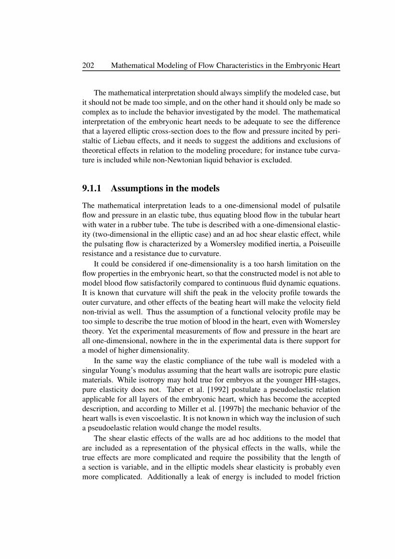
202 Mathematical Modeling of Flow Characteristics in the Embryonic Heart
The mathematical interpretation should always simplify the modeled case, butit should not be made too simple, and on the other hand it should only be made socomplex as to include the behavior investigated by the model. The mathematicalinterpretation of the embryonic heart needs to be adequate to see the differencethat a layered elliptic cross-section does to the flow and pressure incited by peri-staltic of Liebau effects, and it needs to suggest the additions and exclusions oftheoretical effects in relation to the modeling procedure; for instance tube curva-ture is included while non-Newtonian liquid behavior is excluded.
9.1.1 Assumptions in the models
The mathematical interpretation leads to a one-dimensional model of pulsatileflow and pressure in an elastic tube, thus equating blood flow in the tubular heartwith water in a rubber tube. The tube is described with a one-dimensional elastic-ity (two-dimensional in the elliptic case) and an ad hoc shear elastic effect, whilethe pulsating flow is characterized by a Womersley modified inertia, a Poiseuilleresistance and a resistance due to curvature.
It could be considered if one-dimensionality is a too harsh limitation on theflow properties in the embryonic heart, so that the constructed model is not able tomodel blood flow satisfactorily compared to continuous fluid dynamic equations.It is known that curvature will shift the peak in the velocity profile towards theouter curvature, and other effects of the beating heart will make the velocity fieldnon-trivial as well. Thus the assumption of a functional velocity profile may betoo simple to describe the true motion of blood in the heart, even with Womersleytheory. Yet the experimental measurements of flow and pressure in the heart areall one-dimensional, nowhere in the in the experimental data is there support fora model of higher dimensionality.
In the same way the elastic compliance of the tube wall is modeled with asingular Young’s modulus assuming that the heart walls are isotropic pure elasticmaterials. While isotropy may hold true for embryos at the younger HH-stages,pure elasticity does not. Taber et al. [1992] postulate a pseudoelastic relationapplicable for all layers of the embryonic heart, which has become the accepteddescription, and according to Miller et al. [1997b] the mechanic behavior of theheart walls is even viscoelastic. It is not known in which way the inclusion of sucha pseudoelastic relation would change the model results.
The shear elastic effects of the walls are ad hoc additions to the model thatare included as a representation of the physical effects in the walls, while thetrue effects are more complicated and require the possibility that the length ofa section is variable, and in the elliptic models shear elasticity is probably evenmore complicated. Additionally a leak of energy is included to model friction

Chapter 9: Discussion and Final Remarks 203
in the walls, thus the shear elasticity is not modeled as a pure elastic effect. Insection 5.6.2 it is demonstrated how the exclusion of the shear effects will alter themodel and simulations considerably; the removal of the friction will un-dampenthe flow, while removal of the shear elasticity altogether will change the effects ofthe pressure waves in addition.
In the embedded tube model the inclusion of the elastic effects of the cardiacjelly is again modeled as a pure elastic effect, and that is probably much too sim-ple. Firstly the elastic response will be given by a complicated interplay betweenbulk and shear modulus given by the geometry of the tube and the elastic tensorof the jelly. Secondly the stress-strain relationship is given by the pseudoelasticequation by Taber et al. [1992]. Thirdly the elasticity is probably followed withfrictional effects just as for the shear elasticity, a fitting addition to the modelwould be to introduce a resistance alongside the capacitance of the cardiac jelly.
Additionally it was seen in section 8.2.2 that the compliance of the cardiacjelly dampen the contractions of the tube, such that the maximum contraction ofthe outer layer is reduced for the contraction of the inner layer. This reflects anentirely physical behavior as some of the energy from the contractions is stored aspotential energy in the cardiac jelly (and some of the energy may be lost to frictionas explained above). The potential energy of the cardiac jelly will subsequentlybe released when the heart relaxes, thus the cardiac jelly will help the contractedheart return to its uncontracted state (actually this is a function of the elasticity ofall the layers in the tubular heart).
The inertial effects of the flow is modified with Womersley theory to includethe velocity profile of pulsatile flow according to the assumption of a periodicpressure gradient in the Navier-Stokes equations. The effect of Womersley the-ory is investigated in section 5.6.1, and mostly consists of a shift of the frequencyspectrum. However, the velocity profile may be further changed by the composi-tion of the blood.
Blood is a two component liquid consisting blood plasma and blood cells.Blood cells can be modeled as ellipsoid deformable bodies in the liquid, and ithas been proven that under a Poiseuille parabolic flow profile they will migratetowards the center of the tube and in doing that they will flatten the parabolicflow profile [Meier, 1987]. This affects the apparent inertia of the blood and insome models this is approximated with a velocity dependent viscosity coefficient,though it is not known how it affects flow with a Womersley profile.
The Womersley theory states that a standard Poiseuille resistance to the flow isused in addition to the inertial effects. It is surprising then that so many objectionsto the Poiseuille equation is regularly given by researchers in the field (see the listin section 3.4).

204 Mathematical Modeling of Flow Characteristics in the Embryonic Heart
The Poiseuille resistance is a function of the viscosity, which is included as aconstant in the modeling even though the high shear effect described in section 3.1should be considered in respect to the diameter of the embryonic heart. Hu et al.[1991] reports a viscosity of 3.8·10−3 Pa·s for embryonic blood though it is notmentioned if this is in consideration of the high shear effect. This effect, which isalso known as the Fahraeus-Lindqvist effect, can alter the viscosity with a factor1.5 to 2 depending on blood hematocrit number [Meier, 1987]. The effect is afunction of the shear rates in the liquid, which are proportional to the slope of thevelocity profile and under the given circumstances could probably be transformedto a function of the frequency of pulsations, and thus this effect could be added tothe model as an viscosity correction factor, just as the Womersley theory gives theinertia correction factor, ψ.
The resistance to flow due to the curvature of the tube is made from engineer-ing principles of the class of effects known as minor losses. The inclusion of thetheory follows the procedure given by Crane Co. [1982] and Keller [1978], yet itis surprising how much effect the curvature has on the flow in the investigationin section 5.6.3. It may be that curvature has a very strong effect on the Liebaueffect, which relies on a mismatch of pulsations to produce a mean flow, thus pul-sating momentum is important in both cases, yet this does not fit with the picturethat curvature is so often ignored in other models of the Liebau effect.
In addition the elliptic models and certainly the embryonic heart open up forsources of minor losses. For the embryonic heart the branching of arteries isimportant. For the elliptic model the twisting of the elliptic cross-section alongthe length of the tube will be a source for minor losses, while with regards tothe curvature it makes a difference how the tube curves in relation to the ellipticcross-section. These effects are not included in the model as they are believed tobe of minor influence to the character of the flow in the embryonic heart.
Finally the pumping mechanism is crudely made, both in the models of theembryonic heart and in the models of Liebau’s ring. For the model of Liebau’sring equations are included in the simulation routine to overwrite the differentialequations of the dynamic radius in the affected sections of the model. This isdone to make an exact replication of the pumping mechanism applied by Ottesen[2003], and yet it is clear from the comparison in section 5.5 that the division intosections of the model partly ruins this emulation of sinusoidal functions used byOttesen.
For the embryonic heart the pumping mechanism is made as concentric con-tractions of the outer layer of the embedded model used in the simulations. Thisis done though the derivative of the contraction functions specified in section 7.4,which is simply added to the rate of change of the major axis specified by equa-tion 6.124. The concentric contractions are an approximation, it is specified byMänner et al. [2009] that the outer layer does exhibit concentric contraction, and

Chapter 9: Discussion and Final Remarks 205
furthermore it is specified by Damon et al. [2009] that the contraction is not sym-metric around the middle axis of the tube, instead the tube at the outer curvatureof the looping heart contracts more than at the inner curvature. These asymmetriccontraction effects are ignored for simplicity reasons.
9.1.2 The simulation routine
It is proven by the simulation of Liebau’s ring that the computation time of thesimulations is essentially short. Considering the feat done by the ‘ode45’ solver inMatLab v. 7.5 (copyright The MathWorks Inc.) it is remarkably fast; the Runge-Kutta iteration of more than hundred differential equations is impressive work.
This is however only when conditions for the ‘ode45’ solver are favorable. Inthe event that the setup of the model state conditions that are too complicated forthe solver, for instance if it needs to check for divergence of equations, the solveris suddenly transformed to a very slow process as it constantly seeks to take lessertime steps and recheck its process. In that instance a routine that under favorableconditions would be done in an hour suddenly takes days to complete.
This problem has especially dampened the procedures with the elliptic modelusing the χ factor that includes shear effects of the tube wall, defined in equation6.96, and the simulations of the embryonic heart. As a result simulation data fromthese routines are not achieved.
During preliminary tests of the models different pumping mechanisms wereemployed, for instance periodic increase in outside pressure, as well as the pump-ing mechanisms presented in chapter 5. It is clear that different pumping mecha-nisms work differently in the simulations, some are easy for the simulation routineto work with while others require much more computation time.
9.1.3 The energy bond technique
The methods employed in the modeling in this thesis proves the strengths of theenergy bond technique. For many the formalism used in the technique may beunfamiliar and appear unnecessary complicated, yet the rules of the energy bondtechnique are given by simple linear relations that are easily comprehensible andthrough the connections of the energy bonds create possibilities for very compli-cated models. Furthermore the energy bond graphs gives a method to visualize theequations of the model, and with some practice they can be interpreted directly inplace of equations.
Yet the greatest strength of the energy bond technique is the modular construc-tion of models, which is something almost unique for the technique. It makes itpossible to concentrate on singular effects of the pulsatile flow in elastic tubes oneat the time during modeling, as long as it is remembered to follow the rules of the

206 Mathematical Modeling of Flow Characteristics in the Embryonic Heart
energy bond technique, which specify how elements are connected such that phys-ical consistency in conserved. Therefore the modeling process in chapter 4 and 6is designed as a stepwise procedure starting with a simple principal structure ofthe model, which is continuously expanded with more effects and in section 9.1.1above even more expansions are suggested.
The same modular construction plays a part when the model is tested in sec-tion 5.6. Each of the elements in the model can be picked out and examined toinvestigate what effect exactly this addition to the model has on the observed flowand pressure. In this way the simulations of the model becomes and active step inthe model construction process, by testing model additions it is easily seen if theyare made correctly and correctly included in the model. If not, they can be easilyreformulated, reconnected or removed from the model.
The simulation step in the construction of the model can be a necessity as themodular construction of models in the energy bond technique is also one of themajor weaknesses in the technique. Other modeling techniques are typically re-lated to a set of assumptions for the specific model, which for instance would givea set of differential equations that are solved to construct the model. Compared tothis the energy bonds are abstract and potentially out of touch with the underlyingassumptions in the model.
For instance the energy bond model in this case makes an implicit assumptionof the discretization of the fluid dynamical equations. The equations are discretein space through the division into sections of the tube, where flow and pressure inthe middle of a section and flow is measured between two neighboring sections.Furthermore the equations are discrete in relation to the modular construction ofthe model, such that one element models inertia and another resistance and so on.To make sure that the equations of the model are correlated to the fluid dynamicalequations it is investigated in section 4.5 how the model equations look in the con-tinuous limit when the length of a section becomes infinitesimal. It is seen that themodel equations converge to the continuity equation and the Euler equation thusproving that the model is a true discretization of the fluid dynamical equations.
9.2 Simulations of the embryonic heart
The simulations of the embryonic heart were expected to state a proof of conceptthat the embryonic heart could in fact be modeled with the models in this thesis.This proof has changed form to a suggestion; it may be possible to model theembryonic heart with the models, but it is not possible to simulate the effects inthe heart. At least not at present.

Chapter 9: Discussion and Final Remarks 207
During the setup many assumptions were made pertaining to the dimensionsand function of the embryonic heart, in fact the function of distribution of the car-diac jelly inside the heart tube visible in figure 7.7 is made from one single mea-surement of cardiac jelly thickness, the rest is guesswork. Therefore the simula-tions can never be anything more than a proof of principle; compared to measureddata of flow and pressure in the embryonic heart from table 8.1 the simulationscould indicate that the models capture the phenomena of the embryonic heart.
If the models should ever be used to model actual flow and pressure of theembryonic heart, measurement data is required. The lack of measurement datafor the embryonic heart is problematic, despite impressing imaging techniquesis employed in the study of embryonic hearts simple physical measurements oflengths and diameters are hard to find.
The setup of the embryonic heart simulations does not require many or con-siderably complicated material parameters; primarily the viscosity and density ofblood and an elastic Young’s modulus for each layer of the tube, which shouldall be possible to measure. In addition a set of dimensional measurements arerequired and an estimation of pumping function and boundary conditions. Thesetup in chapter 7 is reconstructed from various reports but it would increase thesimulation value if all parameters could be obtained from one source.
The modeling and setup of simulations of the embryonic heart is a work thathas never been attempted with this level of detail before, it is very disappointingthat the simulations were not able to complete the task.
9.2.1 Problems in simulation of the embryonic heart
The explanation for the lack of simulation results is simple; the program routinein MatLab is simply not able to produce any results with the present configurationof the models. The reason for the lack of results is more complicated and maycome from several sources.
It is proved in section 8.2.2 that the embedded model works perfectly underthe configuration of Liebau’s ring, so it is clear that the fault does not lie with themodel itself. The only other option is that the problem lies with the setup of theembryonic heart simulations.
In principle four things are differently from the setup of the embryonic heartto the setup of Liebau’s ring, following the simulation setup procedure in chapter5 and 7 the four things are: the parameter estimation, the boundary conditions, thetracing of the tube, and the pumping mechanism.
The parameter estimation is naturally different. The embryonic heart is muchsmaller and the elastic modules much less than for the case of Liebau’s ring, whiledensity and viscosity is about the same. Specifically the elastic modulus of thecardiac jelly deserves attention. In the setup of the embryonic heart the measured

208 Mathematical Modeling of Flow Characteristics in the Embryonic Heart
values for the elastic modulus from table 7.7 are used, which are from one halfto one fifth of the corresponding elastic modules of the myocardial layer. In thesetup of the embedded Liebau’s ring the assumption by Zamir et al. [2003] is used,stating that the cardiac jelly should have an elastic modulus about one tenth of themyocardial layer. Despite this, it is not believed that this could be the cause of theproblems.
The boundary conditions are different but should not be the cause for anycomputation difficulties, in fact it is probably the simulations of Liebau’s ring thathave the most complicated boundary in the form of the cyclic boundary condition.For the embryonic heart the boundary condition at the arterial end includes twoadditional differential equations to the computation, but they are both very simpleand should hardly be the cause for any problems.
The difference in the tracing of the tubes in the embryonic heart and the Liebaumodel is in the radial dimensions of the tube; the rubber tubes in Liebau’s ring hasuniform radius or axial lengths, while the tubular heart tapers towards the arterialend of the tube and for higher HH-stages it even has several bulges. The axiallengths of the embryonic heart tubes are demonstrated by the staircase functionsin figure 7.7. In principle a tube with changing cross-sectional dimensions shouldnot be a problem for the model, not even for the shear elasticity that is designedfor changing axial dimensions. However when the flow and pressure generated bycontraction in a wide part of the tube reaches tube sections that are substantiallythinner, numerical problems may cause the Runge-Kutta algorithm to take smallertime steps. This could be one reason for the problems. Yet when a simulationwith an untapering tube defined with mean values of the dimensions in figure 7.7is attempted, the problem persists, the same is the case for an uncurving tube.
Finally the pumping mechanism is fundamentally different between the twomodel setups; for Liebau’s ring the pumping mechanism is a typical Liebau pumpthat only affects a short length of the tube, while the embryonic heart has a pump-ing mechanism that contracts a large part of the tube and potentially acts as aperistaltic pump. In the simulation of the Liebau model the pumping mechanismis implemented by letting the equations of the pump overwrite the differentialequations of the outer radius in the affected tube sections, it was seen that thiscauses mismatch problems in those sections so for the embryonic heart the pump-ing function is implemented differently. Instead of overwriting the equations forthe outer radius of the tube, the derivative of the pumping equation, defined in bythe functions in figure 7.7, is added to the differential equation of the outer radiusand iterated in the Runge-Kutta algorithm.
This should create a more smooth working pumping mechanism compared tothe simulations of Liebau’s ring, though perhaps the part of the pumping functionin figure 7.7 where the heart actively dilates following the contraction should havebeen omitted from the function. The elasticity of the layered tube should be able

Chapter 9: Discussion and Final Remarks 209
to produce a relaxation to back to the initial position through passive release ofpotential energy, an active dilation function may cause artificial effects where theheart dilates more than it should.
Furthermore the contraction of the outer layer of the tube may cause situationsin the tube where the inner lumen comes close to occlusion, especially in thesections where the cardiac jelly takes up more space of the cross-sectional area.Total occlusion is not possible in the model, except though numerical error in theRunge-Kutta algorithm. Thus when the length of the minor elliptical axis comescloser to zero the computational routine will reduce time steps and activate itsbuilt-in algorithm to check for convergence of the solutions.
A combination of the tapering embedded tube and the application of the pump-ing mechanism may be the cause of the problems for the ‘ode45’ solver in MatLab.The effects will cause the program to reduce the time steps to very small numberswhile convergence is checked by special routines in the solver. In the end this willcreate immense amounts of data that MatLab handles by creating swap disks onthe computer, storing and loading data from those is extremely time consuming.
It was assumed a priori in chapter 1 that the model could produce peristalticflow without problems, yet in the analysis of the problems of the simulationsit seems that this is exactly what causes the problems: A peristaltic contractionfunction that nearly closes the lumen, traveling on a tapering tube.
9.3 Simulations of Liebau’s ring
Contrary to the simulations of the embryonic heart the simulations of Liebau’sring work without problems. A computation of Liebau’s ring withN = 60 sectionand 100 periods takes about 30 minutes when loaded up to the server used for thecomputations in this thesis. This proves that the models themselves are functionaland with the right setup MatLab has no problems with running the simulations.
In section 5.5 it was attempted to validate the simulations of the cylindricLiebau’s ring in relation to reported data by Ottesen [2003] and Snitker et al.[2000], this comparison was only partly successful. It was made clear that thesimulation results compared fairly to the reported data by Ottesen, at least forsmall values of the compression ratio, but none of the simulations were able toreproduce the experimental results by Snitker et al. [2000]. Interestingly whenLiebau’s ring was setup with the elliptic model the eccentric pumping mechanismgiven by equation 8.2 and 8.3 easily reproduced the experimental data for an el-liptic tube with eccentricity 0.1 (almost circular).
The difference is the pumping mechanism; none of the pumping functionsemployed in the simulations in chapter 5 could produce flow to match the ex-perimental results, apparently the eccentric deformation used in chapter 8 can.
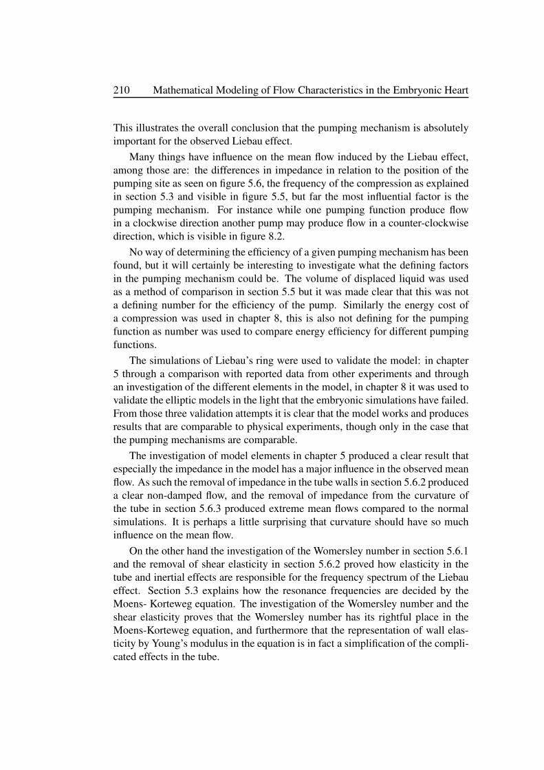
210 Mathematical Modeling of Flow Characteristics in the Embryonic Heart
This illustrates the overall conclusion that the pumping mechanism is absolutelyimportant for the observed Liebau effect.
Many things have influence on the mean flow induced by the Liebau effect,among those are: the differences in impedance in relation to the position of thepumping site as seen on figure 5.6, the frequency of the compression as explainedin section 5.3 and visible in figure 5.5, but far the most influential factor is thepumping mechanism. For instance while one pumping function produce flowin a clockwise direction another pump may produce flow in a counter-clockwisedirection, which is visible in figure 8.2.
No way of determining the efficiency of a given pumping mechanism has beenfound, but it will certainly be interesting to investigate what the defining factorsin the pumping mechanism could be. The volume of displaced liquid was usedas a method of comparison in section 5.5 but it was made clear that this was nota defining number for the efficiency of the pump. Similarly the energy cost ofa compression was used in chapter 8, this is also not defining for the pumpingfunction as number was used to compare energy efficiency for different pumpingfunctions.
The simulations of Liebau’s ring were used to validate the model: in chapter5 through a comparison with reported data from other experiments and throughan investigation of the different elements in the model, in chapter 8 it was used tovalidate the elliptic models in the light that the embryonic simulations have failed.From those three validation attempts it is clear that the model works and producesresults that are comparable to physical experiments, though only in the case thatthe pumping mechanisms are comparable.
The investigation of model elements in chapter 5 produced a clear result thatespecially the impedance in the model has a major influence in the observed meanflow. As such the removal of impedance in the tube walls in section 5.6.2 produceda clear non-damped flow, and the removal of impedance from the curvature ofthe tube in section 5.6.3 produced extreme mean flows compared to the normalsimulations. It is perhaps a little surprising that curvature should have so muchinfluence on the mean flow.
On the other hand the investigation of the Womersley number in section 5.6.1and the removal of shear elasticity in section 5.6.2 proved how elasticity in thetube and inertial effects are responsible for the frequency spectrum of the Liebaueffect. Section 5.3 explains how the resonance frequencies are decided by theMoens- Korteweg equation. The investigation of the Womersley number and theshear elasticity proves that the Womersley number has its rightful place in theMoens-Korteweg equation, and furthermore that the representation of wall elas-ticity by Young’s modulus in the equation is in fact a simplification of the compli-cated effects in the tube.

Chapter 9: Discussion and Final Remarks 211
Finally the investigations of the total number of sections in the model, N ,revealed that there are some differences in the simulation results. This was es-pecially seen in the calculation of the mean flow, which differed a great deal.The explanation is given by the pumping mechanism used in the simulations, be-cause of the different number of sections the pumping mechanism also had to beimplemented differently. Furthermore from preliminary investigations of modelstability it is found that the results are stable when N is high enough so that thelength of one section is comparable to the diameter of the tube.
The results from the simulations of Liebau’s ring proved that comparabilityof the simulations is only possible when pumping mechanisms are comparable,and that the pumping mechanism by far is the most important factor for the ob-served Liebau effect. In turn the simulations validate the model both in respect todifferent effects in the tube and in relation to results by other authors.
9.4 Elliptic vs. circular cross-section
The second of the three questions posed in chapter 1 is answered by use of thesimulations of the elliptic Liebau’s ring: In relation to the possible pumping mech-anisms of the embryonic heart are elliptic contractions of the heart tube optimalcompared to concentric contractions?
According to Männer et al. [2010] it has already been suggested by resultsfrom other researchers that peristaltic pumping has favorable conditions with anelliptic cross-section of the tube, which has previously been used as an argumentfor the peristaltic pumping of the embryonic heart. Though a similar investigationhas not been done for the Liebau effect.
Thus to answer this question a comparison between the Liebau generated flowin elliptic and circular tubes is needed, as well as a comparison between the Liebaugenerated flow induced by concentric and eccentric pumping mechanism. Such acomparison is made with the simulations of Liebau’s ring.
Starting with the question if tubes with elliptic cross-section give better condi-tions for the Liebau effect compared to circular cross-section. The Liebau effectis defined by the pumping mechanism employed, for a cylindric tube with con-centric deformation the mean flow was −1.78 cm3/s, while for a elliptic tube withconcentric deformation the flow was −1.59 cm3/s. Furthermore the mean flowin the elliptic tube decreases with the increase of eccentricity of the ellipse asdemonstrated by figure 8.3. Thus in the simple situation the elliptic cross-sectiondoes not appear to be an advantage for the Liebau effect.
When considering a layered tube with an inner elliptic lumen and outer circu-lar mantle comparable to the cross-section of the embryonic heart, it is seen thatthe mean flow is generally lower than what can be produced in a cylindric tube

212 Mathematical Modeling of Flow Characteristics in the Embryonic Heart
with cross-section comparable to the lumen of the layered tube and with concen-tric contraction. However the mean flow produced in the layered tube dependson the eccentricity of the elliptic inner lumen, an as figure 8.5 demonstrates aneccentricity around 0.4 is optimal for the flow. Thus for the embryonic heart itseems there is an advantage for the Liebau effect if the elliptic lumen of the hearthas a specific eccentricity.
The second question if eccentric contraction is optimal compared to concen-tric contraction. Figure 8.2 shows a comparison between simulations for an el-liptic tube with concentric contraction and a similar elliptic tube with eccentricdeformation. It is seen that the eccentric contraction is far superior to the con-centric for all simulated frequencies. Furthermore figure 8.3 shows a comparisonbetween the concentric and eccentric contraction for different configuration of theeccentricity of the elliptic cross-section of the tube. It is seen that even for eccen-tricities going towards the circular limit the eccentric contraction is superior. Forhigh eccentricities an artificial effect of the eccentric deformation makes the re-sults unreliable. Thus the eccentric deformation gives a clear advantage comparedto concentric contraction in this case.
As stated before the Liebau effect is highly dependent on the pumping func-tion and as such another eccentric contraction of the tube may be less effectivecompared to the one demonstrated in this thesis. For instance an obvious choiceof deformation could be that only one elliptical axis is contracted while the otheris kept constant. Thus a conclusive answer can not be given to this question.
9.5 Peristaltic pumping vs. the Liebau effect
The third of the three questions posed in chapter 1 is difficult to answer consid-ering that the simulations of the embryonic heart models did not succeed: Giventhe morphology and cross-sectional shape of the tubular heart will a peristaltic orLiebau pumping principle be desirable for the propagation of blood?
It has been suggested by Liebau [1955] and several others that the Liebaueffect is the mechanism responsible for the flow of blood in the embryonic heartinstead of peristaltic pumping, or that the effect could contribute to the flow. Infact researchers have discovered embryonic hearts in fish that apparently worksolely from a Liebau principle [Männer et al., 2010].
The two hypotheses of the pumping mechanism in the heart have differentobservations speaking for and against them. For the peristaltic pumping the prob-lems are typically that the flow produced by peristaltic waves is continuous, notpulsatile, and that the flow in the embryonic heart supersedes the speed and fre-quency of the peristaltic contraction waves. For the Liebau effect the problemsare typically that the Liebau effect is caused by periodic contractions at a single
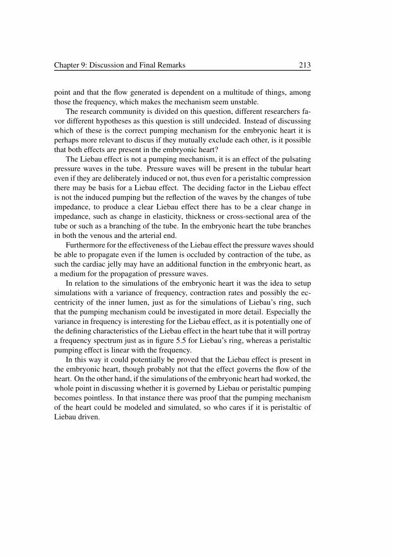
Chapter 9: Discussion and Final Remarks 213
point and that the flow generated is dependent on a multitude of things, amongthose the frequency, which makes the mechanism seem unstable.
The research community is divided on this question, different researchers fa-vor different hypotheses as this question is still undecided. Instead of discussingwhich of these is the correct pumping mechanism for the embryonic heart it isperhaps more relevant to discus if they mutually exclude each other, is it possiblethat both effects are present in the embryonic heart?
The Liebau effect is not a pumping mechanism, it is an effect of the pulsatingpressure waves in the tube. Pressure waves will be present in the tubular hearteven if they are deliberately induced or not, thus even for a peristaltic compressionthere may be basis for a Liebau effect. The deciding factor in the Liebau effectis not the induced pumping but the reflection of the waves by the changes of tubeimpedance, to produce a clear Liebau effect there has to be a clear change inimpedance, such as change in elasticity, thickness or cross-sectional area of thetube or such as a branching of the tube. In the embryonic heart the tube branchesin both the venous and the arterial end.
Furthermore for the effectiveness of the Liebau effect the pressure waves shouldbe able to propagate even if the lumen is occluded by contraction of the tube, assuch the cardiac jelly may have an additional function in the embryonic heart, asa medium for the propagation of pressure waves.
In relation to the simulations of the embryonic heart it was the idea to setupsimulations with a variance of frequency, contraction rates and possibly the ec-centricity of the inner lumen, just as for the simulations of Liebau’s ring, suchthat the pumping mechanism could be investigated in more detail. Especially thevariance in frequency is interesting for the Liebau effect, as it is potentially one ofthe defining characteristics of the Liebau effect in the heart tube that it will portraya frequency spectrum just as in figure 5.5 for Liebau’s ring, whereas a peristalticpumping effect is linear with the frequency.
In this way it could potentially be proved that the Liebau effect is present inthe embryonic heart, though probably not that the effect governs the flow of theheart. On the other hand, if the simulations of the embryonic heart had worked, thewhole point in discussing whether it is governed by Liebau or peristaltic pumpingbecomes pointless. In that instance there was proof that the pumping mechanismof the heart could be modeled and simulated, so who cares if it is peristaltic ofLiebau driven.
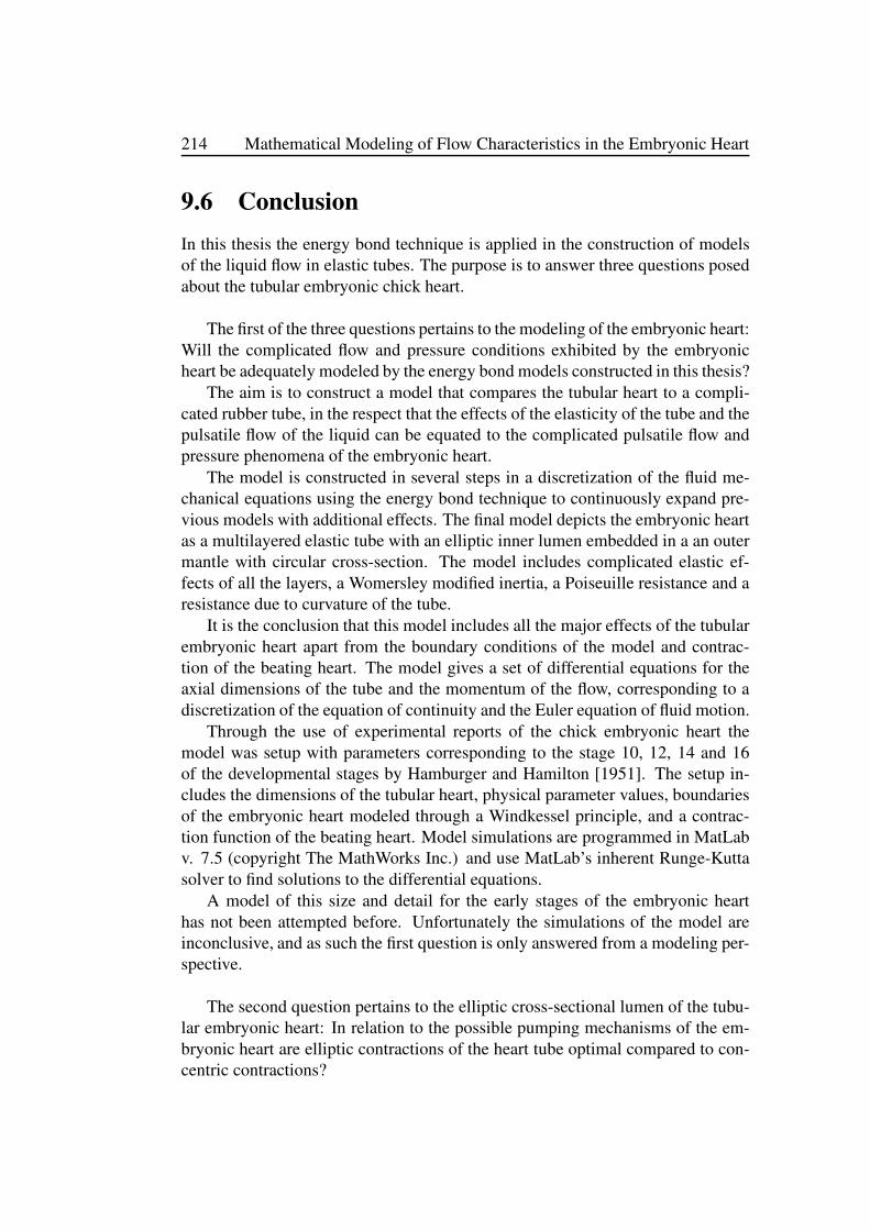
214 Mathematical Modeling of Flow Characteristics in the Embryonic Heart
9.6 Conclusion
In this thesis the energy bond technique is applied in the construction of modelsof the liquid flow in elastic tubes. The purpose is to answer three questions posedabout the tubular embryonic chick heart.
The first of the three questions pertains to the modeling of the embryonic heart:Will the complicated flow and pressure conditions exhibited by the embryonicheart be adequately modeled by the energy bond models constructed in this thesis?
The aim is to construct a model that compares the tubular heart to a compli-cated rubber tube, in the respect that the effects of the elasticity of the tube and thepulsatile flow of the liquid can be equated to the complicated pulsatile flow andpressure phenomena of the embryonic heart.
The model is constructed in several steps in a discretization of the fluid me-chanical equations using the energy bond technique to continuously expand pre-vious models with additional effects. The final model depicts the embryonic heartas a multilayered elastic tube with an elliptic inner lumen embedded in a an outermantle with circular cross-section. The model includes complicated elastic ef-fects of all the layers, a Womersley modified inertia, a Poiseuille resistance and aresistance due to curvature of the tube.
It is the conclusion that this model includes all the major effects of the tubularembryonic heart apart from the boundary conditions of the model and contrac-tion of the beating heart. The model gives a set of differential equations for theaxial dimensions of the tube and the momentum of the flow, corresponding to adiscretization of the equation of continuity and the Euler equation of fluid motion.
Through the use of experimental reports of the chick embryonic heart themodel was setup with parameters corresponding to the stage 10, 12, 14 and 16of the developmental stages by Hamburger and Hamilton [1951]. The setup in-cludes the dimensions of the tubular heart, physical parameter values, boundariesof the embryonic heart modeled through a Windkessel principle, and a contrac-tion function of the beating heart. Model simulations are programmed in MatLabv. 7.5 (copyright The MathWorks Inc.) and use MatLab’s inherent Runge-Kuttasolver to find solutions to the differential equations.
A model of this size and detail for the early stages of the embryonic hearthas not been attempted before. Unfortunately the simulations of the model areinconclusive, and as such the first question is only answered from a modeling per-spective.
The second question pertains to the elliptic cross-sectional lumen of the tubu-lar embryonic heart: In relation to the possible pumping mechanisms of the em-bryonic heart are elliptic contractions of the heart tube optimal compared to con-centric contractions?

Chapter 9: Discussion and Final Remarks 215
With the constructed model the aim is to investigate the difference betweenflow in tubes with circular and elliptic cross-sections as well as flow induced byconcentric and eccentric contractions of the tubes. This should be investigated forthe possible pumping mechanisms of the embryonic heart; peristaltic pumping andthe Liebau effect, though as reports have already been published suggesting thatelliptic tubes may be optimal for peristaltic pumping, focus is put on the Liebaueffect.
By use of a constructed case of two elastic tubes with different elastic modulusjoined together end-to-end to form a ring and filled with water the Liebau effectis investigated for different configurations of pumping mechanisms and cross-sectional shape.
It is concluded from the simulations of this case that a tube with elliptic cross-section gives worse conditions for the Liebau effect than a tube with circular cross-section, and the calculated mean flow of the Liebau effect decreases as eccentric-ity of the ellipse increases. On the other hand when elastic tubes correspondingto the multilayered model of the embryonic heart are setup in this configurationthe simulations demonstrate a peak in the mean flow for an elliptic lumen witheccentricity 0.4. This suggests that for the layered tubular heart the elliptic lumenmay provide advantageous conditions for the Liebau effect.
Through comparison of concentric and eccentric pumping functions for a sys-tem with elliptic tubes it is clear that eccentric contractions produce a mean flowof far higher magnitude. This result persists even for tubes approaching a circularcross-section. In general it is evident that the contraction function is very influ-ential on the observed Liebau effect, in some respects even more influential thanpumping frequency and position of the pump. This suggests that eccentric con-tractions may be optimal for the Liebau effect in the embryonic heart.
The third question pertains to the pumping principle of the tubular embryonicheart: Given the morphology and cross-sectional shape of the tubular heart will aperistaltic or Liebau pumping principle be desirable for the propagation of blood?
With the constructed model and the setup according to the embryonic heartit is the aim to investigate the possible mechanics in the propagation of blood.This would be done through simulations with varying frequency of the heart’spumping mechanism as the effect of peristaltic pumping is linear with frequencywhile the Liebau effect is clearly non-linear and demonstrate resonance effects,thus through investigation of the frequency spectrum it could be decided, whichpumping mechanism is dominant in the models.
As the simulations of the embryonic heart are unsuccessful this approach isnot viable and this question is given only minor attention. It is suggested that thetwo pumping principles are in fact not mutually exclusive and thus both poten-tially could contribute to the propulsion of blood. Nothing in the theory suggests
216 Mathematical Modeling of Flow Characteristics in the Embryonic Heart
that the pumping effects exclude each other, and potentially a function of the lay-ers in the embryonic heart could be to allow for both effects.
The results of this thesis contribute an understanding of the multilayered tubu-lar nature of the embryonic heart that has not been reported earlier. The resultsindicate that the elliptic lumen and the elliptic contraction of the embryonic heartcould potentially optimize conditions for a Liebau pumping phenomena, whileat the same time suggesting that peristaltic pumping and the Liebau effect canco-exist as blood propagation mechanisms in the tubular heart.
The modeling and simulation of the tubular heart of various stages in the earlyembryonic development has never been attempted before in the size and detail asin this thesis, it is concluded that the model includes all major effects pertaining tothe flow and elasticity of the heart tube. As such the modeling has value in itself.Unfortunately the simulations are inconclusive, which is something that has to beremedied in the future.

Bibliography
P. W. Alford and L. A. Taber. Regional epicardial strain in the embryonic chickheart during the early looping stages. Journal of Biomechanics, 36:1135–1141,2003.
Aristotle. Historia Animalum by D’Arcy Wentworth Thompson. Translated byJ.A. Smith and W.D. Ross. Clarendon Press, Oxford, 1910.
K. Azer and C. S. Peskin. A One-dimensional Model of Blood Flow in Arterieswith Friction and Convection Based on the Womersley Velocity Profile. Car-
diovascular Engineering, 7:51–73, 2007.
R. W. Barnard, K. Pearce, and L. Schovanec. Inequalities for the Perimeter ofan Ellipse. Journal of Mathematical Analysis and Applications, 260:295–306,2001.
A. Barry. The Functional Significance of the Cardiac Jelly in the Tubular Heart ofthe Chick Embryo. The Anatomical Record, 102(3):289–298, 1948.
S. Berger, L. Talbot, and L. Yao. Flow in Curved Pipes. Annual Review of Fluid
Mechanics, 15:461–512, 1983.
M. Butlin. Structural and functional effects on large artery stiffness: an in-vivo
experimental investigation. The university of New South Wales, Sydney, 2007.
K. A. Campbell, N. Hu, E. B. Clark, and B. B. Keller. Analysis of DynamicAtrial Dimension and Function during Early Cardiac Development in the ChickEmbryo. Pediatric Research, 32(3):333–337, 1992.
A. Castenholz and T. Flórez-Cossio. Mikrokymographische Untersuchungen zurHerz- und Kreislaufdynamik in der frühen Embryonalentwicklung des Hüh-nchens. In: Altern und Entwicklung, Bd 4. Stuttgart, New York: Akad WissLiterat Mainz, pages 41–61, 1972.
P. V. Christiansen. Imfufa tekst 22: Semiotik og Systemegenskaber (1) - 1-port
lineært response og støj i fysikken. Imfufa, Roskilde University, 1979.
217

218 Mathematical Modeling of Flow Characteristics in the Embryonic Heart
P. V. Christiansen. Imfufa tekst 238: Semiotik og Systemegenskaber (2) - vektor-
bånd og tensorer. Imfufa, Roskilde University, 1993.
P. V. Christiansen. Imfufa tekst 419: Energy bond graphs - a semiotic formaliza-
tion of modern physics. Imfufa, Roskilde University, 2003.
Crane Co. Technical Paper No. 410M: Flow of Fluids - through valves, fittings,
and pipe (Metric edition - SI units). Crane Company, 300 Park Avenue, NewYork, 1982.
B. J. Damon, M. C. Rémond, M. R. Bigelow, T. C. Trusk, W. Xie, R. Perucchio,D. Sedmera, S. Denslow, and R. P. Thompson. Patterns of Muscular Strain inthe Embryonic Heart Wall. Developmental Dynamics, 238:1535–1546, 2009.
A. Davis, J. Izatt, and F. Rothenberg. Quantitative Measurement of Blood FlowDynamics in Embryonic Vasculature Using Spectral Doppler Velocimetry. The
Anatomical Record, 292(3):311–319, 2009.
R. P. Feynman, R. B. Leighton, and M. Sands. The Feynman Lectures on Physics -
The Difinitive Edition, volume II. Addison-Wesley Publishing Company, Read-ing, Massachusetts, 1964. ISBN 0-8053-9047-2.
W. C. Gibson. Celebrating the "compleat observer": William Harvey’s 400thbirthday. Canadian Medical Association Journal, 119(7):793–801, 1978.
R. A. Granger. Fluid Mechanics. Dover Publications, New York, 1995.
J. Hale, D. McDonald, and J. Womersley. Velocity Profiles of Oscillating Arte-rial Flow with some Calculations of Viscous Drag and the Reynolds Number.Journal of Physiology, 128:629–640, 1955.
V. Hamburger and H. L. Hamilton. A Series of Normal Stages in the Developmentof the Chick Embryo. Journal of Morphology, 88(1):49–92, 1951.
R. Hoeben. Experimental investigations into the role of impedence defined flow
during CPR, (MSc thesis). Eindhoven University of Technology, Departmentof Biomedical Engineering, 2009.
N. Hu and E. B. Clark. Hemodynamics of the stage 12 to stage 29 chick embryo.Circulation Research, 65:1665–1670, 1989.
N. Hu, D. M. Connuck, B. B. Keller, and E. B. Clark. Diastolic Filling Charater-istics in the Stage 12 to 27 Chick Embryo Ventricle. Pediatric Research, 29(4):334–337, 1991.

Bibliography 219
B. Keller, N. Hu, P. Serrino, and E. Clark. Ventricular pressure-area loop charac-teristics in the stage 16 to 24 chick embryo. Circulation Research, 68:226–231,1991.
B. B. Keller, N. Hu, and E. B. Clark. Correlation of ventricular area, perime-ter, and conotruncal diameter with ventricular mass and function in the chickembryo from stages 12 to 24. Circulation Research, 66:109–114, 1990.
G. R. Keller. Hydraulic System Analysis. Editors of Hydraulics & PneumaticsMagazine, Cleveland, 1978.
J. K. Larsen, V. Andreasen, H. Larsen, M. S. Olufsen, and J. T. Ottesen. Cardio-
vascular modelling at IMFUFA from The Way Through Science and Philoso-
phy: Essays in Honour of Stig Andur Pedersen. College Publications, London,2006. ISBN 1-904987-33-8.
K. S. Latacha, M. C. Rémond, A. Ramasubramanian, A. Y. Chen, E. L. Elson, andL. A. Taber. Role of Actin Polymerization in Bending of the Early Heart Tube.Developmental Dynamics, 233:1272–1286, 2005.
B. Lautrup. Physics of Continuous Matter - Exotic and Everyday Phenomena in
the Macroscopic World. Institute of Physics Publishing, 2005. ISBN 0-7503-0752-8.
G. Liebau. Über ein ventilloses Pumpprinzip. Naturwissenschaften, 41(14):327,January 1954.
G. Liebau. Herzpulsation und Blutbewegung. Zeitschrift für die gesamte experi-
mentelle Medizin, 125:482–498, 1955.
I.-E. Lin and L. A. Taber. Mechanical Effects of Looping in the Embryonic ChickHeart. Journal of Biomechanics, 27(3):311–321, 1994.
A. Liu, R. Wang, K. L. Thornburg, and S. Rugonyi. Efficient postacquisition syn-chronization of 4-D nongated cardiac images obtained from optical coherencetomography: application to 4-D reconstruction of the chick embryonic heart.Journal of Biomedical Optics, 14(4):044020, 2009.
C. G. Manopoulos, D. S. Mathioulakis, and S. G. Tsangaris. One-dimensionalmodel of valveless pumping in a closed loop and a numerical solution. Physics
of Fluids, 18(1):017106–16, 2006.
B. J. Martinsen. Reference Guide to the Stages of Chick Heart Embryology.Developmental Dynamics, 233:1217–1237, 2005.

220 Mathematical Modeling of Flow Characteristics in the Embryonic Heart
D. A. McDonald. The Occurence of Turbulent Flow in the Rabbit Aorta. Journal
of Physiology, 118:340–347, 1952.
D. A. McDonald. The Relation of Pulsatile Pressure to Flow in Arteries. Journal
of Physiology, 127:533–552, 1955.
D. A. McDonald. Hemodynamics. Annual Review of Physiology, 30:525–556,1968.
G. Meier. Viscous Flow in the Embryonic Heart Geometry. Embryologische
Hefte, 1:1–19, 1987.
C. Miller, M. Vanni, L. Taber, and B. Keller. Passive Stress-Strain Measurementsin the Stage-16 and Stage-18 Embryonic Chick Heart. Journal of Biomechani-
cal Engineering, 119:445–451, 1997a.
C. E. Miller, M. A. Vanni, and B. B. Keller. Characterization of Passive EmbryonicMyocardium by Quasi-Linear Viscoelastic Theory. Journal of Biomechanics,30(9):985–988, 1997b.
J. Männer. Cardiac Looping in the Chick Embryo: A Morphological ReviewWith Special Reference to Terminological and Biomechanical Aspects of theLooping Process. The Anatomical Record, 259:248–262, 2000.
J. Männer. On Rotation, Torsion, Lateralization and Hnededness of the EmbryonicHeart Loop: New Insights From a Simulation Model for the Heart Loop ofChick Embryos. The Anatomical Record Part A, 278A:481–´492, 2004.
J. Männer. Ontogenetic development of the helical heart: concepts and facts.European Journal of Cardio-thoracic Surgery, 295:S69–S74, 2006.
J. Männer. The Anatomy of Cardiac Looping: A Step Towards the Understandingof the Morphogenesis of Several Forms of Congenital Cardiac Malformations.Clinical Anatomy, 21, 2008.
J. Männer, L. Thrane, K. Norozi, and T. M. Yelbuz. High-Resolution In VivoImaging of the Cross-Sectional Deformations of Contracting Embryonic HeartLoops Using Optical Coherence Tomography. Developmental Dynamics, 237:953–961, 2008.
J. Männer, L. Thrane, K. Norozi, and T. M. Yelbuz. In Vivo Imaging of the CyclicChanges in Cross-sectional Shape of the Ventricular Segment of Pulsating Em-bryonic Chick Hearts at Stages 14 to 17: A Contribution to the Understandingof the Ontogenesis of Cardiac Pumping Function. Developmental Dynamics,238:3273–3284, 2009.

Bibliography 221
J. Männer, A. Wessel, and T. M. Yelbuz. How Does the Tubular Embryonic HeartWork? Looking for the Physical Mechanism Generating Unidirectional BloodFlow in the Valveless Embryonic Heart Tube. Developmental Dynamics, 239:1035–1046, 2010.
W. W. Nichols and M. F. O’Rourke. McDonald’s Blood Flow in Arteries - Theo-
retical, experimental and clinical principles. Arnold, a member of the HodderHeadline Group, London, 4th edition, 1998. ISBN 0-340-64614-4.
W. W. Nichols and M. F. O’Rourke. The life and times of Donald A. McDonald.Artery Research, 2:1–8, 2008.
G. J. Noordergraaf, J. T. Ottesen, W. J. Kortsmit, W. H. Schilders, G. J. Scheffer,and A. Noordergraaf. The Donders Model of the Circulation in Normo- andPathophysiology. Cardiovascular Engineering, 6:53–72, 2006.
T. Nørgaard, J. Ellegaard, J. Jalving, J. B. Pedersen, P. Gregersen, S. I. Meyer,and H. Wittus. Aorta-modellering. 4th semester, Naturvidenskabelig Basis,Roskilde University, 1993.
M. S. Olufsen. Imfufa tekst 419: Modeling the Arterial System with Reference to
an Anestesia Simulator. Imfufa, Roskilde University, 1998.
J. T. Ottesen. Valveless pumping in a fluid-filled closed elastic tube-system: one-dimensional theory with experimental validation. Journal of Mathematical Bi-
ology, 46:309–332, 2003.
B. M. Patten, T. C. Kramer, and A. Barry. Valvular Action in the EmbryonicChick Heart by Localized Apposition of Endocardial Masses. The Anatomical
Record, 102(3):299–311, 1948.
A. Pressley. Elementary Differential Geometry. Springer-Verlag, London, 2001.ISBN 1-85233-152-6.
V. C. Rideout. Mathematical and Computer Modeling of Physiological Systems.Prentice Hall, 1991. ISBN 0-13-563354-0.
A. Snitker, A.-G. Knudsen, H. Skourup, J. Lauridsen, J. Hansen, and K. Olesen.Bestemmelse af flowretning i et lukket elastisk kredsløb. 2nd semester, Naturv-idenskabelig Basis, Roskilde University, 2000.
L. A. Taber. Mechanical aspects of cardiac development. Progress in Biophysics
and Molecular Biology, 69:237–255, 1998.

222 Mathematical Modeling of Flow Characteristics in the Embryonic Heart
L. A. Taber. Biophysical mechanisms of cardiac looping. International Journal
of Developmental Biology, 50:323–332, 2006a.
L. A. Taber. Computational Model for Early Cardiac Looping. Annals of Biomed-
ical Engineering, 34(8):1655–1669, 2006b.
L. A. Taber, B. B. Keller, and E. B. Clark. Cardiac Mechanics in the Stage-16Chick Embryo. Journal of Biomechanical Engineering, 114:427–434, 1992.
L. A. Taber, I. E. Lin, and E. B. Clark. Mechanics of Cardiac Looping. Develop-
mental Dynamics, 203:42–50, 1995.
J. Womersley. Oscillatory Motion of a Viscous Liquid in a Thin-Walled ElasticTube - 1: The Linear Approximation for Long Waves. Philosophical Magazine,46:199–221, 1955a.
J. Womersley. Method for the Calculation of Velocity, Rate of Flow and ViscousDrag in Arteries when the Pressure Gradient is Known. Journal of Physiology,127:553–563, 1955b.
T.-S. Yang and C.-C. Wang. Effects of Actuator Impact on the Nonlinear Dy-namics of a Valveless Pumping System. Journal of Mechanics in Medicine and
Biology, 0(1):1–33, 2010.
T. M. Yelbuz, M. A. Choma, L. Thrane, M. L. Kirby, and J. A. Izatt. Optical Co-herence Tomography: A New High-Resolution Imaging Technology to StudyCardiac Development in Chick Embryos. Circulation, 106:2771–2774, 2002.
M. Yoshigi and B. B. Keller. Linearity of Pulsatile Pressure-Flow Relations in theEmbryonic Chick Vacular System. Circulation Research, 79:864–870, 1996.
M. Yoshigi and B. B. Keller. Characterization of embryonic aortic impedancewith lumped parameter models. American Journal of Physiology, 273(1 pt 2):H19–27, 1997.
M. Yoshigi, G. D. Knott, and B. B. Keller. Lumped parameter estimation forthe embryonic chick vascular system: a time-domain approach using MLAB.Computer Methods and Programs in Biomedicine, 63:29–41, 2000.
K. Zahka, N. Hu, K. Brin, F. Yin, and E. Clark. Aortic impedance and hydraulicpower in the chick embryo from stages 18 to 29. Circulation Research, 64:1091–1095, 1989.

Bibliography 223
E. A. Zamir and L. A. Taber. Material Properties and Residual Stress in the Stage12 Chick Heart During Cardiac Looping. Journal of Biomechanical Engineer-
ing, 126:823–830, 2004.
E. A. Zamir, V. Srinivasan, R. Perucchio, and L. A. Taber. Mechanical Asym-metry in the Embryonic Chick Heart During Looping. Annals of Biomedical
Engineering, 31:1327–1336, 2003.


Appendix A
Simulation Code for Liebau’s Ring
For the simulations of Liebau’s ring the cylindric model presented in chapter 4 isimplemented into MatLab v. 7.5 (copyright The MathWorks Inc.).
The implementation into MatLab requires two separate programs that are re-ferred to as the iterative program and the master program. The master programdefines the material parameters of the tubes and the desired conditions chosen forthe simulation. Specifically the master program initiates the vectors for the dy-namic radius and momentum of the tube, r and p, each containing N elementscorresponding to the number of sections in the model. It then calculates the ele-ments of the model such as capacitance, inductance and resistance and with thosevalues it calls the iterative routine.
MatLab contains an inherent fourth-order Runge-Kutta solver ‘ode45.m’ thatwill handle the time-iteration of the differential equations specified by the model.The ‘ode45’ solver is initiated by the master program and it then subsequentlycalls the iterative program.
The iterative program works in the way that given the values of the vectors rand p it will calculate their derivatives for each section, dr and dp, and returnthem to the Runge-Kutta solver, which will then evaluate these derivatives andgive the iterative program a new set of vectors r and p. This continues for a timeduration set by the master program.
When the time-iteration in the Runge-Kutta solver is completed ‘ode45’ re-turns the vector functions r and p to the master program. These functions arenow transformed to t by N matrices, where t is the number of time-steps doneby the iteration. From those two matrices the master program will calculate thecorresponding functions of pressure and flow, P and Q, with the same dimensionas the r and p.
The rutine is the same in all the programs used in this thesis, and therefore thiswill not be explained again in B and C. The programs are presented below.
225
226 Mathematical Modeling of Flow Characteristics in the Embryonic Heart
The iterative program
% rkliebau.m
% Runge-Kutta iteration of the cylindric model.
% Modification of the model to fit Liebau’s Ring.
function output = rkliebau(t,z)
global N f x R eta f_B C L C_s Z_s;
global psection plength delay Comp;
% Defining radii and momentum from the input vector
r = z(1:N-plength)’;
p = z(N+1-plength:end)’;
% The piston pump
r(psection+plength:N) = r(psection:N-plength);
r_min = sqrt(R(psection:psection+plength-1).^2
- (R(psection:psection+plength-1).^2
- (R(psection:psection+plength-1).* sqrt(1-Comp)).^2)
.* (sin((pi/(plength+1)).*[1:plength])));
for j=1:plength
r(psection+j-1) = R(psection+j-1);
r(psection+j-1) = sqrt(R(psection+j-1)^2
- (R(psection+j-1)^2-r_min(j)^2)
* sin(pi*f/0.1 * (t-delay*(j-1)))
* (0<=mod(t-delay*(j-1),1/f))
* ((0.1/f)>=mod(t-delay*(j-1),1/f)));
end
% Equations for the rate of change of the radii
dr(1) = 1/(2*pi*x*r(1))
* ((p(N)/L(N))*sqrt(r(N)*r(1)/(R(N)*R(1)))
- (p(1)/L(1))*sqrt(r(1)*r(2)/(R(1)*R(2))));
dr(2:N-1) = 1./(2.*pi.*x.*r(2:N-1)).*((p(1:N-2)./L(1:N-2))
.* sqrt(r(1:N-2).*r(2:N-1)./(R(1:N-2).*R(2:N-1)))
- (p(2:N-1)./L(2:N-1))
.*sqrt(r(2:N-1).*r(3:N)./(R(2:N-1).*R(3:N))));
dr(N) = 1/(2*pi*x*r(N)) * ((p(N-1)/L(N-1))
* sqrt(r(N-1)*r(N)/(R(N-1)*R(N)))
- (p(N)/L(N))*sqrt(r(N)*r(1)/(R(N)*R(1))));

Appendix A: Simulation Code for Liebau’s Ring 227
% Equations for the pressure
P(1) = 1/(2*pi*x*r(1)) * ( (r(1)-R(1))/C(1)
+ ((r(1)-R(1))-(r(N)-R(N)))/C_s(N)+Z_s(N)*(dr(1)-dr(N))
- ((r(2)-R(2))-(r(1)-R(1)))/C_s(1)-Z_s(1)*(dr(2)-dr(1))
+ (p(N)^2)/(2*r(1)*L(N)) + (p(1)^2)/(2*r(1)*L(1)) );
P(2:N-1) = 1./(2.*pi.*x.*r(2:N-1))
.* ( (r(2:N-1)-R(2:N-1))./C(2:N-1)
+ ((r(2:N-1)-R(2:N-1))
- (r(1:N-2)-R(1:N-2)))./C_s(1:N-2)
+ Z_s(1:N-2).*(dr(2:N-1)-dr(1:N-2))
- ((r(3:N)-R(3:N))-(r(2:N-1)-R(2:N-1)))./C_s(2:N-1)
- Z_s(2:N-1).*(dr(3:N)-dr(2:N-1))
+ (p(1:N-2).^2)./(2.*r(2:N-1).*L(1:N-2))
+ (p(2:N-1).^2)./(2.*r(2:N-1).*L(2:N-1)) );
P(N) = 1/(2*pi*x*r(N)) * ( (r(N)-R(N))/C(N)
+ ((r(N)-R(N))-(r(N-1)-R(N-1)))/C_s(N-1)
+ Z_s(N-1)*(dr(N)-dr(N-1))
- ((r(1)-R(1))-(r(N)-R(N)))/C_s(N)
- Z_s(N)*(dr(1)-dr(N))
+ (p(N-1)^2)/(2*r(N)*L(N-1))
+ (p(N)^2)/(2*r(N)*L(N)) );
% Equations for the rate of change of the momentum
dp(1) = sqrt(r(1)*r(2)/(R(1)*R(2)))
* ( P(1) - P(2) - ( (8*eta*x)/(pi*r(1)^2*r(2)^2)
+ (f_B(1)*sqrt(R(1)*R(2))
* sign(p(1))*p(1))/(4*pi*r(1)^2*r(2)^2) )
* p(1)/L(1) * sqrt(r(1)*r(2)/(R(1)*R(2))) )
+ (p(1)/(2*r(1)))*dr(1) + (p(1)/(2*r(2)))*dr(2);
dp(2:N-1) = sqrt(r(2:N-1).*r(3:N)./(R(2:N-1).*R(3:N)))
.* ( P(2:N-1) - P(3:N)
- ( (8.*eta.*x)./(pi.*r(2:N-1).^2.*r(3:N).^2)
+ (f_B(2:N-1).*sqrt(R(2:N-1).*R(3:N))
.* sign(p(2:N-1)).*p(2:N-1))
./ (4.*pi.*r(2:N-1).^2.*r(3:N).^2) )
.* p(2:N-1)./L(2:N-1)
.* sqrt(r(2:N-1).*r(3:N)./(R(2:N-1).*R(3:N))) )
+ (p(2:N-1)./(2.*r(2:N-1))).*dr(2:N-1)
+ (p(2:N-1)./(2.*r(3:N))).*dr(3:N);

228 Mathematical Modeling of Flow Characteristics in the Embryonic Heart
dp(N) = sqrt(r(N)*r(1)/(R(N)*R(1)))
* ( P(N) - P(1) - ( (8*eta*x)/(pi*r(N)^2*r(1)^2)
+ (f_B(N)*sqrt(R(N)*R(1))
* sign(p(N))*p(N))/(4*pi*r(N)^2*r(1)^2) )
* p(N)/L(N) * sqrt(r(N)*r(1)/(R(N)*R(1))) )
+ (p(N)/(2*r(N)))*dr(N) + (p(N)/(2*r(1)))*dr(1);
dr = [dr(1:psection-1) dr(psection+plength:N)];
% The output to the main program
output = [dr’;dp’];
The master program
% liebau.m
% A model for pulsating flow in elastic tubes.
% The model is used to simulate Liebau’s Ring.
function liebau
% Initializing variables
global N f x R eta f_B C L C_s Z_s;
global psection plength delay Comp;
r = 0; p = 0; P = 0; Q = 0; R = 0;
% The numbers we can change
N = 60; % The number of sections in the model
psection = 5; % The first section of the pump
plength = 3; % The number of sections of the pump
delay = 0; % The delay time in sequential pumping
Comp = 0.25; % The cross-sectional compression ratio
f = 2.06; %Hz % The frequency of the pump
periods = 50; % The number of periods in the simulation
time = periods * 1/f; %s % The time of the simulation
% The parameters of the tube at rest
l = 1.0; %m % The length of the tube
x = l/N; %m % Length per section
R(1:N/2) = 0.01; %m The radius of the soft tube at rest
R(N/2+1:N) = 0.008; %m The radius of the rigid tube at rest
r(1:N) = R(:); %m % The dynamic radii of the tube
p(1:N) = 0; %kg*m/s % The initial momentum of the flow

Appendix A: Simulation Code for Liebau’s Ring 229
% The curvature of the tube
R_B(1:N) = l/(2*pi); % The bend radius for each section
theta(1:N) = (x.*360)./(2.*pi.*R_B); %deg. % The bend angle
% The physical properties of the tube and the liquid
rho = 1000; %kg/m3 % The density of the liquid (water)
eta = 0.001; %Pa.s % The viscosity of the liquid (water)
P_0 = 1e5; %Pa % The pressure outside the tube
E1 = 4.1e5; %Pa % Young’s modulus for the soft tube
E2 = 4.3e5; %Pa % Young’s modulus for the rigid tube
h1 = 0.001; %m % Wall thickness of the soft tube
h2 = 0.003; %m % Wall thickness of the rigid tube
% Womersley theory
alpha(1:N-1) = sqrt(R(1:N-1).*R(2:N))*sqrt(2*pi*f*rho/eta);
alpha(N) = sqrt(R(N).*R(1)).*sqrt(2*pi*f*rho/eta);
psi = real(1 ./ (1 - 2./(alpha.*sqrt(-i))
.* besselj(1,alpha.*sqrt(-i))
./ besselj(0,alpha.*sqrt(-i))) - 8./(i.*alpha.^2));
% Equations for the curvature of the tube
xi = 0.042 .* theta.^0.69;
K_B(1:N-1) = 9.0704.*(log(R_B(1:N-1)
./ (2.*sqrt(R(1:N-1).*R(2:N))))).^2
- 16.9345.*(log(R_B(1:N-1)
./ (2.*sqrt(R(1:N-1).*R(2:N))))) + 19.6437;
K_B(N) = 9.0704.*(log(R_B(N)./(2.*sqrt(R(N).*R(1))))).^2
- 16.9345.*(log(R_B(N)./(2.*sqrt(R(N).*R(1)))))
+ 19.6437;
f_T(1:N-1) = 0.0478.*(2.*sqrt(R(1:N-1).*R(2:N))).^(-0.2245);
f_T(N) = 0.0478.*(2.*sqrt(R(N).*R(1))).^(-0.2245);
% The calculation of the elements of the model
C(1:N/2) = 1/(2*pi*x*E1*h1) * R(1:N/2); %cm/dyn
C(N/2+1:N) = 1/(2*pi*x*E2*h2) * R(N/2+1:N); %cm/dyn
L(1:N-1) = psi(1:N-1).*rho.*x./(pi*(R(1:N-1).*R(2:N)));
L(N) = psi(N)*rho*x/(pi*R(N)*R(1)); %g/cm4
C_s(1:N/2) = x./(2*pi*(1/3)*E1*h1
* sqrt(R(1:N/2).*R(2:N/2+1))); %cm/dyn
C_s(N/2+1:N-1) = x./(2*pi*(1/3)*E2*h2
* sqrt(R(N/2+1:N-1).*R(N/2+2:N))); %cm/dyn
C_s(N/2) = x./(2*pi*(1/3)*sqrt(E1*h1*E2*h2)
* sqrt(R(N/2)*R(N/2+1))); %cm/dyn
230 Mathematical Modeling of Flow Characteristics in the Embryonic Heart
C_s(N) = x./(2*pi*(1/3)*sqrt(E1*h1*E2*h2)
* sqrt(R(N)*R(1))); %cm/dyn
Z_s(1:N) = 0.01./C_s; %dyn/cm
f_B = xi.*K_B.*f_T./psi; % The friction factor
% Call MatLab’s solver for ordinary differential equations
r = [r(1:psection-1) r(psection+plength:N)];
[t,z] = ode45(’rkliebau’,[0 time],[r p]);
r = z(:,1:N-plength); p = z(:,N+1-plength:end);
% The compression pump
r(1:length(t),psection+plength:N) =
r(1:length(t),psection:N-plength);
r_min = sqrt(R(psection:psection+plength-1).^2
- (R(psection:psection+plength-1).^2
- (R(psection:psection+plength-1).*sqrt(1-Comp)).^2)
.* (sin((pi/(plength+1)).*[1:plength])));
for j=1:plength
r(1:length(t),psection+j-1) = R(psection+j-1);
r(1:length(t),psection+j-1) = sqrt(R(psection+j-1).^2
- (R(psection+j-1).^2-r_min(j).^2)
.* sin(pi*f/0.1 .* (t-delay*(j-1)))
.* (0<=mod(t-delay*(j-1),1/f))
.* ((0.1/f)>=mod(t-delay*(j-1),1/f)));
end
% Calculation of driving pressure and volume flow
T = length(t);
P(1,1:N) = P_0; %Pa % The outside pressure
Q(1,1:N) = 0; %cm3/s % Initial volume flow is set to zero
P(2:T,1) = 1./(2.*pi.*x.*r(2:T,1)) .* ((r(2:T,1)-R(1))./C(1)
+ ((r(2:T,1)-R(1))-(r(2:T,N)-R(N)))./C_s(N)
+ Z_s(N).*((r(2:T,1)-r(1:T-1,1))./(t(2:T)-t(1:T-1))
- (r(2:T,N)-r(1:T-1,N))./(t(2:T)-t(1:T-1)))
- ((r(2:T,2)-R(2))-(r(2:T,1)-R(1)))./C_s(1)
- Z_s(1).*((r(2:T,2)-r(1:T-1,2))./(t(2:T)-t(1:T-1))
- (r(2:T,1)-r(1:T-1,1))./(t(2:T)-t(1:T-1)))
+ (p(2:T,N).^2)./(2.*r(2:T,1).*L(N))
+ (p(2:T,1).^2)./(2.*r(2:T,1).*L(1))) + P_0;

Appendix A: Simulation Code for Liebau’s Ring 231
P(2:T,2:N-1) = 1./(2.*pi.*x.*r(2:T,2:N-1)) .* ((r(2:T,2:N-1)
- ones(T-1,1)*R(2:N-1))./(ones(T-1,1)*C(2:N-1))
+ ((r(2:T,2:N-1)-ones(T-1,1)*R(2:N-1))
- (r(2:T,1:N-2)-ones(T-1,1)*R(1:N-2)))
./ (ones(T-1,1)*C_s(1:N-2))
+ (ones(T-1,1)*Z_s(1:N-2)).*((r(2:T,2:N-1)
- r(1:T-1,2:N-1))./((t(2:T)-t(1:T-1))
* ones(1,N-2))-(r(2:T,1:N-2)-r(1:T-1,1:N-2))
./ ((t(2:T)-t(1:T-1))*ones(1,N-2)))
- ((r(2:T,3:N)-ones(T-1,1)*R(3:N))
- (r(2:T,2:N-1)-ones(T-1,1)*R(2:N-1)))
./ (ones(T-1,1)*C_s(2:N-1))
- (ones(T-1,1)*Z_s(2:N-1)).*((r(2:T,3:N)
- r(1:T-1,3:N))./((t(2:T)-t(1:T-1))
* ones(1,N-2))-(r(2:T,2:N-1)-r(1:T-1,2:N-1))
./ ((t(2:T)-t(1:T-1))*ones(1,N-2)))
+ (p(2:T,1:N-2).^2)./(2.*r(2:T,2:N-1)
.* (ones(T-1,1)*L(1:N-2)))
+ (p(2:T,2:N-1).^2)./(2.*r(2:T,2:N-1)
.* (ones(T-1,1)*L(2:N-1)))) + P_0;
P(2:T,N) = 1./(2.*pi.*x.*r(2:T,N)) .* ((r(2:T,N)-R(N))./C(N)
+ ((r(2:T,N)-R(N))-(r(2:T,N-1)-R(N-1)))./C_s(N-1)
+ Z_s(N-1).*((r(2:T,N)-r(1:T-1,N))
./ (t(2:T)-t(1:T-1))-(r(2:T,N-1)-r(1:T-1,N-1))
./ (t(2:T)-t(1:T-1)))-((r(2:T,1)-R(1))
- (r(2:T,N)-R(N)))./C_s(N)- Z_s(N).*((r(2:T,1)
- r(1:T-1,1))./(t(2:T)-t(1:T-1))-(r(2:T,N)
- r(1:T-1,N))./(t(2:T)-t(1:T-1)))
+ (p(2:T,N-1).^2)./(2.*r(2:T,N).*L(N-1))
+ (p(2:T,N).^2)./(2.*r(2:T,N).*L(N))) + P_0;
Q(2:T,1:N-1) = p(2:T,1:N-1)./(ones(T-1,1)*L(1:N-1))
.* sqrt(r(2:T,1:N-1).*r(2:T,2:N)
./ (ones(T-1,1)*(R(1:N-1).*R(2:N))) );
Q(2:T,N) = p(2:T,N)./L(N) .* sqrt( r(2:T,N).*r(2:T,1)
./ (R(N).*R(1)) );
save ’liebau.mat’ r p P Q t f


Appendix B
Simulation Code for the Tubular
Heart
The simulations of embryonic heart is made similar to the simulations of Liebau’sring following the same procedure as described in appendix A. Each HH-stage ofthe embryo modeled has its own master program detailing the specific conditionsat that stage, but the iterative program applied in the simulations is the same.
The iterative program
% rkembryo.m
% Runge-Kutta iteration of the embedded tubular flow
% model as used in the modeling of chick embryonic hearts.
function output = rkembryo(t,z)
%% Initialization of the cycle
global N x A B; % The dimensions of the tubular heart
global C_sn C_vn C_r C_j L C_sa Z_sa L_c R_c R_p C_p;
global P_0 eta f_B f IFT_con Vent_con OFT_con;
global Pumpsections Pumptimes delay;
% Defining the radii and momentum from the input vector
a = (z(1:N))’; b = (z(N+1:2*N))’; p = (z(2*N+1:end-2))’;
V = z(end-1); M = z(end);
233

234 Mathematical Modeling of Flow Characteristics in the Embryonic Heart
%% Defining variables for the cycle
% Calculation of the elliptic integrals
ecc = sqrt(1 - (min(a,b)./max(a,b)).^2); % eccentricity
first = (pi/2) .* ( 1 + (1/2)^2*ecc.^2 + (3/8)^2*ecc.^4
+ (15/48)^2*ecc.^6 + (105/384)^2*ecc.^8 );
second = (pi/2) .* (1-(1/2)^2*ecc.^2-(1/3)*(3/8)^2*ecc.^4
- (1/5)*(15/48)^2*ecc.^6+(1/7)*(105/384)^2*ecc.^8 );
% Calculation of the surface derivatives
dsda = (a>b).*(x.*(4./((a~=b).*a.^2-b.^2))
.* (a.^2.*second-b.^2.*first)) + (a==b).*x.*pi
+ (a<b).*((4.*b.*a./((a<b).*b.^2-a.^2))
.* (first-second));
dsdb = (a>b).*(x.*(4.*a.*b./((a~=b).*a.^2-b.^2))
.* (first-second)) + (a==b).*x.*pi
+ (a<b).*(x.*(4./((a<b).*b.^2-a.^2))
.* (b.^2.*second-a.^2.*first));
% Calculation of the chi factor
chi = ( ((b./a).*dsdb.^2-dsda.*dsdb)./C_sn
+ 2.*((2.*a.*b)./(a.^2+b.^2)).^2.*(1./(a.*b)).*(1./C_vn)
+ (pi*x)^2.*2.*a.^2./C_j )
./ ( (dsda.^2-(b./a).*dsda.*dsdb)./C_sn
+ 2.*((2.*a.*b)./(a.^2+b.^2)).^2.*(1./a.^2).*(1./C_vn)
+ (pi*x)^2.*2.*a.*(2.*a-b)./C_j + 1./C_r );
%% The pumping mechanism
% Pumping is made by contracting the outer radius
% by means of derivative of the contraction function
% dr = -pi abc R_0 exp(-ct) cos(pi b(1-exp(-ct))
time(1:N) = (t-delay*((1:N)-Pumpsections(1))); dr(1:N) = 0;
dr(Pumpsections(1):Pumpsections(2)) =
- pi*IFT_con(1)*IFT_con(2)*IFT_con(3)
.* A(Pumpsections(1):Pumpsections(2))
.* exp(-IFT_con(3).*time(Pumpsections(1):Pumpsections(2)))
.* cos(pi.*IFT_con(2).*(1-exp(-IFT_con(3)
.* time(Pumpsections(1):Pumpsections(2)))))
.* (0<=mod(time(Pumpsections(1):Pumpsections(2)),1/f))
.* (Pumptimes(1)>=mod(time(Pumpsections(1)
: Pumpsections(2)),1/f));

Appendix B: Simulation Code for the Tubular Heart 235
dr(Pumpsections(2):Pumpsections(3)) =
- pi*Vent_con(1)*Vent_con(2)*Vent_con(3)
.* A(Pumpsections(2):Pumpsections(3)).*exp(-Vent_con(3)
.* time(Pumpsections(2):Pumpsections(3)))
.* cos(pi.*Vent_con(2).*(1-exp(-Vent_con(3)
.* time(Pumpsections(2):Pumpsections(3)))))
.* (0<=mod(time(Pumpsections(2):Pumpsections(3)),1/f))
.* (Pumptimes(2)>=mod(time(Pumpsections(2)
: Pumpsections(3)),1/f));
dr(Pumpsections(3):Pumpsections(4)) =
- pi*OFT_con(1)*OFT_con(2)*OFT_con(3)
.* A(Pumpsections(3):Pumpsections(4))
.* exp(-OFT_con(3).*time(Pumpsections(3):Pumpsections(4)))
.* cos(pi.*OFT_con(2).*(1-exp(-OFT_con(3)
.* time(Pumpsections(3):Pumpsections(4)))))
.* (0<=mod(time(Pumpsections(3):Pumpsections(4)),1/f))
.* (Pumptimes(3)>=mod(time(Pumpsections(3)
: Pumpsections(4)),1/f));
%% Calculation of model variables
% Calculation of the flow
Q(1) = (p(1)/L(1)) * sqrt( (sqrt(a(1)*A(1))*sqrt(b(1)*B(1)))
/ (A(1)*B(1)) );
Q(2:N) = (p(2:N)./L(2:N))
.* sqrt( (sqrt(a(1:N-1).*a(2:N))
.* sqrt(b(1:N-1).*b(2:N)))./(sqrt(A(1:N-1).*A(2:N))
.* sqrt(B(1:N-1).*B(2:N))) );
Q(N+1) = M/L_c;
% Equations for the rate of change of the axes
da = (Q(1:N)-Q(2:N+1))/(pi*x) .* (chi./(a+chi.*b)) + dr;
db = (Q(1:N)-Q(2:N+1))/(pi*x) .* (1./(a+chi.*b));
% Equations for the dynamic pressure
P(1) = (1/(pi*x*b(1))) * ( (a(1)-A(1))/C_r(1)
+ dsda(1)*(dsda(1)*(a(1)-A(1))/C_sn(1)
+ dsdb(1)*(b(1)-B(1))/C_sn(1))
+ ((2*a(1)*b(1))/(a(1)^2+b(1)^2))*(1/a(1))
* tan(((2*a(1)*b(1))/(a(1)^2+b(1)^2))
* ((1/a(1))*(a(1)-A(1))/C_vn(1)-(1/b(1))
* (b(1)-B(1))/C_vn(1)))-(x*pi)^2*(2*a(1)-b(1))
* ((2*a(1)-b(1))*(a(1)-A(1))/C_j(1)

236 Mathematical Modeling of Flow Characteristics in the Embryonic Heart
- a(1)*(b(1)-B(1))/C_j(1))
+ (a(1)-A(1))/C_sa(1) + Z_sa(1)*da(1)
- ((a(2)-A(2))-(a(1)-A(1)))/C_sa(2)
- Z_sa(2)*(da(2)-da(1))
+ (p(1)^2)/(4*a(1)*L(1)) + (p(2)^2)/(4*a(1)*L(2)) );
P(2:N-1) = (1./(pi.*x.*b(2:N-1)))
.* ( (a(2:N-1)-A(2:N-1))./C_r(2:N-1)
+ dsda(2:N-1).*(dsda(2:N-1).*(a(2:N-1)
- A(2:N-1))./C_sn(2:N-1) + dsdb(2:N-1).*(b(2:N-1)
- B(2:N-1))./C_sn(2:N-1))
+ ((2.*a(2:N-1).*b(2:N-1))./(a(2:N-1).^2
+ b(2:N-1).^2)).*(1./a(2:N-1))
.* tan(((2.*a(2:N-1).*b(2:N-1))./(a(2:N-1).^2
+ b(2:N-1).^2)).*((1./a(2:N-1))
.*(a(2:N-1)-A(2:N-1))./C_vn(2:N-1)
- (1./b(2:N-1)).*(b(2:N-1)-B(2:N-1))./C_vn(2:N-1)))
- (x*pi).^2.*(2.*a(2:N-1)-b(2:N-1))
.* ((2.*a(2:N-1)-b(2:N-1)).*(a(2:N-1)-A(2:N-1))
./ C_j(2:N-1)-a(2:N-1).*(b(2:N-1)-B(2:N-1))
./ C_j(2:N-1))+((a(2:N-1)-A(2:N-1))
- (a(1:N-2)-A(1:N-2)))./C_sa(2:N-1)
+ Z_sa(2:N-1).*(da(2:N-1)-da(1:N-2))
- ((a(3:N)-A(3:N))-(a(2:N-1)-A(2:N-1)))./C_sa(3:N)
- Z_sa(3:N).*(da(3:N)-da(2:N-1))
+ (p(2:N-1).^2)./(4.*a(2:N-1).*L(2:N-1))
+ (p(3:N).^2)./(4.*a(2:N-1).*L(3:N)) );
P(N) = (1/(pi*x*b(N))) * ( (a(N)-A(N))/C_r(N)
+ dsda(N)*(dsda(N)*(a(N)-A(N))/C_sn(N)
+ dsdb(N)*(b(N)-B(N))/C_sn(N))
+ ((2*a(N)*b(N))/(a(N)^2+b(N)^2))*(1/a(N))
* tan(((2*a(N)*b(N))/(a(N)^2+b(N)^2))
* ((1/a(N))*(a(N)-A(N))/C_vn(N)-(1/b(N))*(b(N)-B(N))
/ C_vn(N)))-(x*pi)^2*(2*a(N)-b(N))*((2*a(N)-b(N))
* (a(N)-A(N))/C_j(N) - a(N)*(b(N)-B(N))/C_j(N))
+ ((a(N)-A(N))-(a(N-1)-A(N-1)))/C_sa(N)
+ Z_sa(N)*(da(N)-da(N-1))
+ (a(N)-A(N))/C_sa(N+1)
+ Z_sa(N+1)*da(N) + (p(N)^2)/(4*a(N)*L(N)) );
P(N+1) = V/C_p - P_0;
% Equations for the rate of change of the momentum
dp(1) = sqrt(sqrt(A(1)*a(1))*sqrt(B(1)*b(1))/(A(1)*B(1)))
* ( P_0 - P(1) - ( (4*eta*x*(A(1)*a(1)+B(1)*b(1)))

Appendix B: Simulation Code for the Tubular Heart 237
/ (sqrt(A(1)*a(1))^3*sqrt(B(1)*b(1))^3)
+ (f_B(1)*(1/(4*pi))*sqrt(A(1)*B(1)/(sqrt(A(1)*a(1))^5
* sqrt(B(1)*b(1))^5))*sqrt((A(1)*a(1)+B(1)*b(1))/2)
* sign(p(1))*p(1)) ) * Q(1) ) + (p(1)/(4*a(1)))*da(1)
+ (p(1)/(4*b(1)))*db(1);
dp(2:N) = sqrt(sqrt(a(1:N-1).*a(2:N)).*sqrt(b(1:N-1).*b(2:N))
./ (sqrt(A(1:N-1).*A(2:N)).*sqrt(B(1:N-1).*B(2:N))))
.* ( P(1:N-1) - P(2:N) - ( (4.*eta.*x.*(a(1:N-1)
.* a(2:N)+b(1:N-1).*b(2:N)))
./ (sqrt(a(1:N-1).*a(2:N)).^3
.* sqrt(b(1:N-1).*b(2:N)).^3)
+ (f_B(2:N).*(1./(4.*pi))
.* sqrt(sqrt(A(2:N).*A(1:N-1).*B(2:N).*B(1:N-1))
./ (sqrt(a(2:N).*a(1:N-1)).^5
.* sqrt(b(2:N).*b(1:N-1)).^5))
.* sqrt((a(2:N).*a(1:N-1)+b(2:N).*b(1:N-1))./2)
.* sign(p(2:N)).*p(2:N)) ) .* Q(2:N) )
+ (p(2:N)./(4.*a(1:N-1))).*da(1:N-1)
+ (p(2:N)./(4.*a(2:N))).*da(2:N)
+ (p(2:N)./(4.*b(1:N-1))).*db(1:N-1)
+ (p(2:N)./(4.*b(2:N))).*db(2:N);
% Equations for the windkessel termination
dV = Q(N+1) - P(N+1)/R_p; dM = P(N) - P(N+1) - Q(N+1)*R_c;
% The output to the main program
output = [da’;db’;dp’;dV;dM];

238 Mathematical Modeling of Flow Characteristics in the Embryonic Heart
The hh10 master program
% hh10.m
% A model of blood flow of a HH-stage 10 embryonic heart.
% The flow model is based on the embedded tube model.
function hh10
%% Initialization of the model
global N x A B; % The dimensions of the tubular heart
global C_sn C_vn C_r C_j L C_sa Z_sa L_c R_c R_p C_p;
global P_0 eta f_B f IFT_con Vent_con OFT_con;
global Pumpsections Pumptimes delay;
a = 0; b = 0; p = 0; P = 0; Q = 0;
N = 30; % The number of sections in the model
% Acceptable numbers = [1 2 3 5 6 8 10 11 15 22 30 33 55 66]
f = 1.0; %Hz % The frequency of the pump
% Frequencies measured = [0.8 1.0 1.2];
periods = 3; % The number of periods in the simulation
time = periods * 1/f; %seconds % The time of the simulation
%% Tracing of the heart loop
% Lengths
L_Sinus_venosis = 50e-6; %m
L_Left_ventricle = 130e-6; %m
L_Right_ventricle = 250e-6; %m
L_Proximal_outflow_tract = 230e-6; %m
% Diameters
D_Sinus_venosis = 330e-6; %m
D_Venous_pole = 300e-6; %m
D_Central_left_ventricle = 270e-6; %m
D_Left_lateral_furrow = 250e-6; %m
D_Central_right_ventricle = 250e-6; %m
D_Conoventricular_sulcus = 200e-6; %m
D_Proximal_outflow_tract = 170e-6; %m
D_Arterial_outlet = 120e-6; %m

Appendix B: Simulation Code for the Tubular Heart 239
% Layers
h_my = 18e-6; %m % The thickness of the myocardial layer
h_cj = 52e-6; %m % The thickness of the cardiac jelly
h_en = h_my/2; %m % The thickness of the endocardial layer
% Dimension setup
tubelength = L_Sinus_venosis + L_Left_ventricle
+ L_Right_ventricle + L_Proximal_outflow_tract;
lengths = [0 L_Sinus_venosis
L_Sinus_venosis+L_Left_ventricle/2
L_Sinus_venosis+L_Left_ventricle
L_Sinus_venosis+L_Left_ventricle+L_Right_ventricle/2
L_Sinus_venosis+L_Left_ventricle+L_Right_ventricle
L_Sinus_venosis+L_Left_ventricle
+L_Right_ventricle+L_Proximal_outflow_tract/2
tubelength];
diameters = [D_Sinus_venosis D_Venous_pole
D_Central_left_ventricle D_Left_lateral_furrow
D_Central_right_ventricle D_Conoventricular_sulcus
D_Proximal_outflow_tract D_Arterial_outlet];
relative_cardiac_jelly = [0.8 0.9 0.9 1.1 1 1.4 1.3 1.1]
* (h_cj/(D_Central_right_ventricle/2));
x = tubelength/N; %m % The length of a section of the tube
% The major and minor axis of the model
l_array = 0:10^(-6):tubelength;
for d=1:length(diameters)-1
coef = polyfit(lengths(d:d+1),diameters(d:d+1)/2,1);
a_array((10^6*lengths(d)+1):(10^6*lengths(d+1)+1)) =
polyval(coef,l_array((10^6*lengths(d)+1)
:(10^6*lengths(d+1)+1)));
coef = polyfit(lengths(d:d+1),(diameters(d:d+1)/2)
.* (1-relative_cardiac_jelly(d:d+1)),1);
b_array((10^6*lengths(d)+1):(10^6*lengths(d+1)+1)) =
polyval(coef,l_array((10^6*lengths(d)+1)
:(10^6*lengths(d+1)+1)));
end
for n=1:N
index = uint16(((n-1)*x+x/2)*10^6);
A(n) = a_array(index); %m % The major axis of at rest
B(n) = b_array(index); %m % The minor axis of at rest
end

240 Mathematical Modeling of Flow Characteristics in the Embryonic Heart
a(1:N) = A(1:N); %m % The dynamic major axis of the tube
b(1:N) = B(1:N); %m % The dynamic minor axis of the tube
% Curvature
R_B(1:N) = 550e-6; %m % The radius of curvature
startindex = find(x*(1:N)>L_Sinus_venosis,1,’first’);
endindex = find(x*(1:N)>L_Sinus_venosis
+ L_Left_ventricle+L_Right_ventricle
+ (1/4)*L_Proximal_outflow_tract,1,’first’);
theta(1:N) = 0; %deg. % The bending angle for each section
theta(startindex:endindex) = (x./(2.*pi
.* R_B(startindex:endindex))).*360;
% Boundary conditions
P_0 = 26.7; %Pa % The mean pressure at the venous end
L_c = 14.87e8; %kg/m4 % Inertance of the vascular system
R_c = 5.41e11; %Pa.s/m3 % Characteristic resistance
R_p = 10.74e11; %Pa.s/m3 % Peripheral resistance
C_p = 0.31e-12; %m3/Pa % Capacitance of the vascular system
V_0 = P_0*C_p; %m3 % Equilibrium vascular system volume
V = V_0; %m3 % The dynamical volume of the vascular system
M = 0; %Pa.s % The momentum through the vascular system
%% Parameter estimation
% The physical parameters of the heart tube and the blood
rho = 1.0e3; %kg/m3 % The density of embryonic blood
eta = 3.8e-3; %Pa.s % The viscosity of embryonic blood
E_my = 60; %Pa % Young’s modulus for the myocardial layer
E_cj = 12; %Pa % Young’s modulus for the cardiac jelly
E_en = E_my; %Pa % Young’s modulus for the endocardial layer
%% The pumping mechanism
p(1:N) = 0; %kg*m/s % The initial momentum of the flow
T_prox_contraction = 170.0e-3; %s % Proximal contraction
T_dist_contraction = 228.0e-3; %s % Distal contraction
T_prox_relaxation = 275.6e-3; %s % Proximal relaxation
T_dist_relaxation = 286.0e-3; %s % Distal relaxation
Wave_velocity = 3.3e-3; %m/s % Contraction wave velocity
Diametric_contraction = 0.15; % Diametric contraction ratio

Appendix B: Simulation Code for the Tubular Heart 241
% Tracing of the contraction functions
% Given by: X(t) = 1 - a*sin(pi*b*(1-exp(-c*time)))
IFT_con = [0.4287 1.3480 0.001015];
Vent_con = [0.3329 1.0635 0.001418];
OFT_con = [0.3072 6.6597 0.00006598];
IFT_con(1) = (Diametric_contraction/Vent_con(1))
* IFT_con(1);
OFT_con(1) = (Diametric_contraction/Vent_con(1))
* OFT_con(1);
Vent_con(1) = (Diametric_contraction/Vent_con(1))
* Vent_con(1);
IFT_con(3) = -log((Vent_con(2)-1)/Vent_con(2))
/ (T_prox_contraction+T_prox_relaxation)
* (IFT_con(3)/Vent_con(3));
Vent_con(3) = -log((Vent_con(2)-1)/Vent_con(2))
/ (T_prox_contraction+T_prox_relaxation);
OFT_con(3) = -log((OFT_con(2)-1)/OFT_con(2))
/ (T_dist_contraction+T_dist_relaxation);
% Defining the contraction durations
IFT_time = (-1/IFT_con(3))*log((IFT_con(2)-1)/IFT_con(2));
Vent_time = (-1/Vent_con(3))
* log((Vent_con(2)-1)/Vent_con(2));
OFT_time = (-1/OFT_con(3))*log((OFT_con(2)-1)/OFT_con(2));
Pumptimes = [IFT_time Vent_time OFT_time];
% Defining the contraction zones
IFT_section = find(x*(1:N)>L_Sinus_venosis,1,’first’);
Vent_section = find(x*(1:N)>L_Sinus_venosis,1,’first’);
OFT_section = find(x*(1:N)>L_Sinus_venosis+L_Left_ventricle
+ L_Right_ventricle,1,’first’);
End_section = find(x*(1:N)>L_Sinus_venosis+L_Left_ventricle
+ L_Right_ventricle+(1/2)
* L_Proximal_outflow_tract,1,’first’);
Pumpsections = [IFT_section Vent_section
OFT_section End_section];
% Defining the phase shift between sections
delay = x/Wave_velocity;
242 Mathematical Modeling of Flow Characteristics in the Embryonic Heart
%% The model engine
% Calculated characteristics of the elliptic tube
S(1:N) = x*pi*(A+B).*(1+3*((A-B)./(A+B)).^2.
/ (10+sqrt(4-3*((A-B)./(A+B)).^2))); %m2
Omega(1) = pi.*(A(1)+B(1)).*(1
+ 3*((A(1)-B(1))./(A(1)+B(1))).^2./(10
+ sqrt(4-3.*((A(1)-B(1))./(A(1)+B(1))).^2))); %m
Omega(2:N) = pi.*(sqrt(A(1:N-1).*A(2:N))+sqrt(B(1:N-1)
.* B(2:N))).*(1+3*((sqrt(A(1:N-1).*A(2:N))
- sqrt(B(1:N-1).*B(2:N)))./(sqrt(A(1:N-1)
.* A(2:N))+sqrt(B(1:N-1).*B(2:N)))).^2./(10
+ sqrt(4-3.*((sqrt(A(1:N-1).*A(2:N))
- sqrt(B(1:N-1).*B(2:N)))./(sqrt(A(1:N-1)
.* A(2:N))+sqrt(B(1:N-1).*B(2:N)))).^2)) ); %m
Omega(N+1) = pi.*(A(N)+B(N)).*(1
+ 3*((A(N)-B(N))./(A(N)+B(N))).^2./(10
+ sqrt(4-3.*((A(N)-B(N))./(A(N)+B(N))).^2))); %m
% Womersley theory
alpha(1) = sqrt((2*A(1)^2*B(1)^2)/(A(1)^2+B(1)^2))
* sqrt(2*pi*f*rho/eta);
alpha(2:N) = sqrt((2.*A(1:N-1).*A(2:N).*B(1:N-1).*B(2:N))
./ (A(1:N-1).*A(2:N)+B(1:N-1).*B(2:N)))
.* sqrt(2*pi*f*rho/eta);
psi = real(1 ./ (1 - 2./(alpha.*sqrt(-i))
.* besselj(1,alpha.*sqrt(-i))
./ besselj(0,alpha.*sqrt(-i))) - 8./(i.*alpha.^2));
% Equations for the curvature of the tube
xi = 0.042 .* theta.^0.69;
l_c(1) = sqrt(2*A(1)^2*B(1)^2 / (A(1)^2+B(1)^2)); %m
l_c(2:N) = sqrt(2.*A(1:N-1).*A(2:N).*B(1:N-1).*B(2:N)
./ (A(1:N-1).*A(2:N)+B(1:N-1).*B(2:N))); %m
K_B(1:N) = 9.0704.*(log(R_B(1:N)./(2.*l_c(1:N)))).^2
- 16.9345.*(log(R_B(1:N)./(2.*l_c(1:N))))+19.6437;
f_T(1:N) = 0.0478.*(2.*l_c(1:N)).^(-0.2245);
f_B = xi.*K_B.*f_T./psi;
% The calculation of the primary elements of the model
C_sn(1:N) = S./(E_en.*h_en); %m/Pa=m3/N
C_vn(1:N) = 1./(S.*(1/3).*E_en.*h_en); %(Pa.m3)^-1=(N.m)^-1
C_r(1:N) = 1./(pi*x*E_my*h_my) .* (A(1:N)); %(Pa.m)^-1=m/N

Appendix B: Simulation Code for the Tubular Heart 243
C_j(1:N) = (pi.*x.*(A(1:N).^2-A(1:N).*B(1:N)))./E_cj; %m3/Pa
L(1) = psi(1)*rho*x./(pi*A(1).*B(1)); %kg/m4
L(2:N) = psi(2:N).*rho.*x./(pi.
* sqrt(A(1:N-1).*A(2:N).*B(1:N-1).*B(2:N))); %kg/m4
% The calculation of the shear elements of the network model
C_sa(1) = 2.*x ./ ( (1/3).*E_en.*h_en.*Omega(1)
+ 4.*pi.*(1/3).*E_my.*h_my.*A(1) ); %(Pa.m)^-1=m/N
C_sa(2:N) = 2.*x ./ ( (1/3).*E_en.*h_en.*Omega(2:N) + 4.*pi
.* (1/3).*E_my.*h_my.*sqrt(A(1:N-1).*A(2:N)) );
C_sa(N+1) = 2.*x ./ ( (1/3).*E_en.*h_en.*Omega(N+1)
+ 4.*pi.*(1/3).*E_my.*h_my.*A(N) ); %(Pa.m)^-1=m/N
C_sb(1:N+1) = 2.*x ./ ( (1/3).*E_en.*h_en.*Omega(1:N+1) );
Z_sa(1:N+1) = 0.01./C_sa; %Pa.m=N/m
Z_sb(1:N+1) = 0.01./C_sb; %Pa.m=N/m
%% The Runge-Kutta algorithm
% Call MatLab’s solver for ordinary differential equations
options = odeset(’RelTol’,1e-3,’AbsTol’,1e-6,’Stats’,’on’);
[t,z] = ode45(’rkembryo’,[0 time],[a b p V M],options);
a = z(:,1:N); b = z(:,N+1:2*N); p = z(:,2*N+1:end-2);
V = z(:,end-1); M = z(:,end);
%% Calculation of flow and pressure
T = length(t);
% Calculation of the elliptic integrals
ecc = sqrt(1-(min(a,b)./max(a,b)).^2); % Eccentricity
first = (pi/2).*(1+(1/2)^2*ecc.^2+(3/8)^2*ecc.^4
+ (15/48)^2*ecc.^6+(105/384)^2*ecc.^8);
second = (pi/2).*(1-(1/2)^2*ecc.^2-(1/3)*(3/8)^2*ecc.^4
- (1/5)*(15/48)^2*ecc.^6+(1/7)*(105/384)^2*ecc.^8);
% Calculation of the surface derivatives
dsda = (a>b).*(x.*(4./((a>b).*a.^2-b.^2))
.* (a.^2.*second-b.^2.*first))+(a==b).*x.*pi+(a<b)
.* ((4.*b.*a./((a<b).*b.^2-a.^2)).*(first-second));
dsdb = (a>b).*(x.*(4.*a.*b./((a<b).*a.^2-b.^2))
.* (first-second))+(a==b).*x.*pi+(a<b).*(x.*(4./((a<b)
.* b.^2-a.^2)).*(b.^2.*second-a.^2.*first));

244 Mathematical Modeling of Flow Characteristics in the Embryonic Heart
% Calculation of the dynamic pressure
P(1,1:N+1) = 0; %Pa % Initial pressure is set to zero
P(2:T,1) = 1./(pi.*x.*b(2:T,1)) .* ((a(2:T,1)-A(1))./C_r(1)
+ dsda(2:T,1).*(dsda(2:T,1).*(a(2:T,1)-A(1))
./ C_sn(1)+dsdb(2:T,1).*(b(2:T,1)-B(1))./C_sn(1))
+ ((2.*a(2:T,1).*b(2:T,1))./(a(2:T,1).^2
+ b(2:T,1).^2)).*(1./a(2:T,1)).*tan(((2.*a(2:T,1)
.* b(2:T,1))./(a(2:T,1).^2+b(2:T,1).^2))
.* ((1./a(2:T,1)).*(a(2:T,1)-A(1))./C_vn(1)
- (1./b(2:T,1)).*(b(2:T,1)-B(1))./C_vn(1)))
+ (x.*pi).^2.*(2.*a(2:T,1)-b(2:T,1))
.* ((2.*a(2:T,1)-b(2:T,1))
.* (a(2:T,1)-A(1))./C_j(1)-a(2:T,1).*(b(2:T,1)
- B(1))./C_j(1)) + (a(2:T,1)-A(1))./C_sa(1)
+ Z_sa(1).*(a(2:T,1)-a(1:T-1,1))./(t(2:T)
- t(1:T-1))-((a(2:T,2)-A(2))-(a(2:T,1)-A(1)))
./ C_sa(2)-Z_sa(2).*((a(2:T,2)-a(1:T-1,2))
./ (t(2:T)-t(1:T-1))-(a(2:T,1)-a(1:T-1,1))
./ (t(2:T)-t(1:T-1)))+(p(2:T,1).^2)./(4.*a(2:T,1)
.* L(1))+(p(2:T,2).^2)./(4.*a(2:T,1).*L(2)));
P(2:T,2:N-1) = 1./(pi.*x.*b(2:T,2:N-1)) .* ((a(2:T,2:N-1)
- ones(T-1,1)*A(2:N-1))./(ones(T-1,1)*C_r(2:N-1))
+ dsda(2:T,2:N-1).*(dsda(2:T,2:N-1).*(a(2:T,2:N-1)
- ones(T-1,1)*A(2:N-1))./(ones(T-1,1)*C_sn(2:N-1))
+ dsdb(2:T,2:N-1).*(b(2:T,2:N-1)-ones(T-1,1)
* B(2:N-1))./(ones(T-1,1)*C_sn(2:N-1)))+((2
.* a(2:T,2:N-1).*b(2:T,2:N-1))./(a(2:T,2:N-1).^2
+ b(2:T,2:N-1).^2)).*(1./a(2:T,2:N-1))
.* tan(((2.*a(2:T,2:N-1).*b(2:T,2:N-1))
./ (a(2:T,2:N-1).^2+b(2:T,2:N-1).^2))
.* ((1./a(2:T,2:N-1)).*(a(2:T,2:N-1)-ones(T-1,1)
* A(2:N-1))./(ones(T-1,1)*C_vn(2:N-1))
- (1./b(2:T,2:N-1)).*(b(2:T,2:N-1)-ones(T-1,1)
* B(2:N-1))./(ones(T-1,1)*C_vn(2:N-1))))
+ (x.*pi).^2.*(2.*a(2:T,2:N-1)-b(2:T,2:N-1))
.* ((2.*a(2:T,2:N-1)-b(2:T,2:N-1)).*(a(2:T,2:N-1)
- ones(T-1,1)*A(2:N-1))./(ones(T-1,1)*C_j(2:N-1))
- a(2:T,2:N-1).*(b(2:T,2:N-1)-ones(T-1,1)
* B(2:N-1))./(ones(T-1,1)*C_j(2:N-1)))
+ ((a(2:T,2:N-1)-ones(T-1,1)*A(2:N-1))
- (a(2:T,1:N-2)-ones(T-1,1)*A(1:N-2)))
./ (ones(T-1,1)*C_sa(2:N-1))+(ones(T-1,1)
* Z_sa(2:N-1)).*((a(2:T,2:N-1)-a(1:T-1,2:N-1))

Appendix B: Simulation Code for the Tubular Heart 245
./ ((t(2:T)-t(1:T-1))*ones(1,N-2))-(a(2:T,1:N-2)
- a(1:T-1,1:N-2))./((t(2:T)-t(1:T-1))*ones(1,N-2)))
- ((a(2:T,3:N)-ones(T-1,1)*A(3:N))-(a(2:T,2:N-1)
-ones(T-1,1)*A(2:N-1)))./(ones(T-1,1)*C_sa(3:N))
+ (ones(T-1,1)*Z_sa(3:N)).*((a(2:T,3:N)
- a(1:T-1,3:N))./((t(2:T)-t(1:T-1))*ones(1,N-2))
- (a(2:T,2:N-1)-a(1:T-1,2:N-1))./((t(2:T)-t(1:T-1))
* ones(1,N-2)))+(p(2:T,2:N-1).^2)./(4*a(2:T,2:N-1)
.* (ones(T-1,1)*L(2:N-1))) + (p(2:T,3:N).^2)
./ (4*a(2:T,2:N-1).*(ones(T-1,1)*L(3:N))));
P(2:T,N) = 1./(pi.*x.*b(2:T,N)) .* ((a(2:T,N)-A(N))./C_r(N)
+ dsda(2:T,N).*(dsda(2:T,N).*(a(2:T,N)-A(N))
./ C_sn(N)+dsdb(2:T,N).*(b(2:T,N)-B(N))./C_sn(N))
+ ((2.*a(2:T,N).*b(2:T,N))./(a(2:T,N).^2
+ b(2:T,N).^2)).*(1./a(2:T,N)).*tan(((2.*a(2:T,N)
.* b(2:T,N))./(a(2:T,N).^2+b(2:T,N).^2))
.* ((1./a(2:T,N)).*(a(2:T,N)-A(N))./C_vn(N)
- (1./b(2:T,N)).*(b(2:T,N)-B(N))./C_vn(N)))
+ (x.*pi).^2.*(2.*a(2:T,N)-b(2:T,N))
.* ((2.*a(2:T,N)-b(2:T,N)).*(a(2:T,N)-A(N))
./ C_j(N)-a(2:T,N).*(b(2:T,N)-B(N))./C_j(N))
+ ((a(2:T,N)-A(N))-(a(2:T,N-1)-A(N-1)))./C_sa(N)
+ Z_sa(N).*((a(2:T,N)-a(1:T-1,N))./(t(2:T)
- t(1:T-1))-(a(2:T,N-1)-a(1:T-1,N-1))./(t(2:T)
- t(1:T-1)))+(a(2:T,N)-A(N))./C_sa(N+1)
+ Z_sa(N+1).*(a(2:T,N)-a(1:T-1,N))./(t(2:T)
- t(1:T-1)) + (p(2:T,N).^2)./(4.*a(2:T,N).*L(N)));
P(2:T,N+1) = V(2:T)./C_p-P_0;
% Calculation of the flow
Q(1,1:N+1) = 0; %m3/s % Initial volume flow is set to zero
Q(2:T,1) = p(2:T,1)./L(1) .* sqrt( (sqrt(a(2:T,1).*A(1))
.* sqrt(b(2:T,1).*B(1))) ./ (A(1)*B(1)) );
Q(2:T,2:N) = p(2:T,2:N)./(ones(T-1,1)*L(2:N))
.* sqrt( (sqrt(a(2:T,1:N-1).*a(2:T,2:N))
.* sqrt(b(2:T,1:N-1).*b(2:T,2:N)))
./ (ones(T-1,1)*(sqrt(A(1:N-1).*A(2:N))
.*sqrt(B(1:N-1).*B(2:N)))) );
Q(2:T,N+1) = M(2:T)./L_c;
% Model output
save ’hh10.mat’ t a b p P Q V M f

246 Mathematical Modeling of Flow Characteristics in the Embryonic Heart
The hh12 master program
% hh12.m
% A model for blood flow of a HH-stage 12 embryonic heart.
% The flow model is based on the embedded tube model.
function hh12
%% Initialization of the model
global N x A B; % The dimensions of the tubular heart
global C_sn C_vn C_r C_j L C_sa Z_sa L_c R_c R_p C_p;
global P_0 eta f_B f IFT_con Vent_con OFT_con;
global Pumpsections Pumptimes delay;
a = 0; b = 0; p = 0; P = 0; Q = 0;
N = 29; % The number of sections in the model
% Acceptable numbers = [1 2 4 5 10 20 29 58 97 116]
f = 1.5; %Hz % The frequency of the pump
% Frequencies measured = [1.25 1.32 1.72 1.90];
periods = 3; % The number of periods in the simulation
time = periods * 1/f; %seconds % The time of the simulation
%% Tracing of the heart loop
% Lengths
L_Sinus_venosis = 70e-6; %m
L_Primitive_atrium = 200e-6; %m
L_Left_ventricle = 270e-6; %m
L_Right_ventricle = 370e-6; %m
L_Proximal_outflow_tract = 250e-6; %m
% Diameters
D_Sinus_venosis = 350e-6; %m
D_Venous_pole = 330e-6; %m
D_Central_atrium = 320e-6; %m
D_Upper_atrium = 280e-6; %m
D_lower_left_ventricle = 250e-6; %m
D_Central_left_ventricle = 250e-6; %m
D_Left_lateral_furrow = 250e-6; %m
D_Central_right_ventricle = 230e-6; %m

Appendix B: Simulation Code for the Tubular Heart 247
D_Upper_right_ventricle = 170e-6; %m
D_Conoventricular_sulcus = 150e-6; %m
D_Proximal_outflow_tract = 150e-6; %m
D_Distal_outflow_tract = 150e-6; %m
D_Arterial_outlet = 130e-6; %m
% Layers
h_my = 15e-6; %m % The thickness of the myocardial layer
h_cj = 70e-6; %m % The thickness of the cardiac jelly
h_en = h_my/2; %m % The thickness of the endocardial layer
% Dimension setup
tubelength = L_Sinus_venosis+L_Primitive_atrium
+ L_Left_ventricle+L_Right_ventricle
+ L_Proximal_outflow_tract;
lengths = [0 L_Sinus_venosis L_Sinus_venosis
+3*L_Primitive_atrium/8 L_Sinus_venosis
+6*L_Primitive_atrium/8 L_Sinus_venosis
+L_Primitive_atrium+L_Left_ventricle/3
L_Sinus_venosis+L_Primitive_atrium
+2*L_Left_ventricle/3 L_Sinus_venosis
+L_Primitive_atrium+L_Left_ventricle
L_Sinus_venosis+L_Primitive_atrium
+L_Left_ventricle+4*L_Right_ventricle/10
L_Sinus_venosis+L_Primitive_atrium
+L_Left_ventricle+7*L_Right_ventricle/10
L_Sinus_venosis+L_Primitive_atrium
+L_Left_ventricle+L_Right_ventricle
L_Sinus_venosis+L_Primitive_atrium
+L_Left_ventricle+L_Right_ventricle
+2*L_Proximal_outflow_tract/5
L_Sinus_venosis+L_Primitive_atrium
+L_Left_ventricle+L_Right_ventricle
+9*L_Proximal_outflow_tract/15 tubelength];
diameters = [D_Sinus_venosis D_Venous_pole D_Central_atrium
D_Upper_atrium D_lower_left_ventricle
D_Central_left_ventricle D_Left_lateral_furrow
D_Central_right_ventricle
D_Upper_right_ventricle
D_Conoventricular_sulcus
D_Proximal_outflow_tract
D_Distal_outflow_tract D_Arterial_outlet];

248 Mathematical Modeling of Flow Characteristics in the Embryonic Heart
relative_cardiac_jelly = [0.7 0.9 0.8 0.7 0.9 0.9 1 1 1
1.35 1.3 1.1 1.1] * (h_cj
/(D_Central_right_ventricle/2));
x = tubelength/N; %m % The length of a section of the tube
% The major and minor axis of the model
l_array = 0:10^(-6):tubelength;
for d=1:length(diameters)-1
coef = polyfit(lengths(d:d+1),diameters(d:d+1)/2,1);
a_array((10^6*lengths(d)+1):(10^6*lengths(d+1)+1)) =
polyval(coef,l_array((10^6*lengths(d)+1)
:(10^6*lengths(d+1)+1)));
coef = polyfit(lengths(d:d+1),(diameters(d:d+1)/2)
.*(1-relative_cardiac_jelly(d:d+1)),1);
b_array((10^6*lengths(d)+1):(10^6*lengths(d+1)+1)) =
polyval(coef,l_array((10^6*lengths(d)+1)
:(10^6*lengths(d+1)+1)));
end
for n=1:N
index = uint16(((n-1)*x+x/2)*10^6);
A(n) = a_array(index); %m % The major axis at rest
B(n) = b_array(index); %m % The minor axis at rest
end
a(1:N) = A(1:N); %m % The dynamic major axis of the tube
b(1:N) = B(1:N); %m % The dynamic minor axis of the tube
% Curvature
R_B(1:N) = 500e-6; %m % The radius of curvature
startindex = find(x*(1:N)>L_Sinus_venosis,1,’first’);
endindex = find(x*(1:N)>L_Sinus_venosis+L_Primitive_atrium
+ L_Left_ventricle+L_Right_ventricle+(1/4)
* L_Proximal_outflow_tract,1,’first’);
theta(1:N) = 0; %deg. % The bending angle for each section
theta(startindex:endindex) = (x./(2.*pi
.* R_B(startindex:endindex))).*360;
%% Boundary conditions
P_0 = 26.7; %Pa % The mean pressure at the venous end
L_c = 6.52e8; %kg/m4 % Inertance of the vascular system
R_c = 3.55e11; %Pa.s/m3 % Characteristic resistance
R_p = 9.62e11; %Pa.s/m3 % Peripheral resistance
C_p = 0.36e-12; %m3/Pa % Capacitance of the vascular system

Appendix B: Simulation Code for the Tubular Heart 249
V_0 = P_0*C_p; %m3 % Equilibrium vascular system volume
V = V_0; %m3 % The dynamical volume of the vascular system
M = 0; %Pa.s % The momentum through the vascular system
%% Parameter estimation
% The physical parameters of the heart tube and the blood
rho = 1.0e3; %kg/m3 % The density of embryonic blood
eta = 3.8e-3; %Pa.s % The viscosity of embryonic blood
E_my = 66.6; %Pa % Young’s modulus for the myocardial layer
E_cj = 18; %Pa % Young’s modulus for the cardiac jelly
E_en = E_my; %Pa % Young’s modulus for the endocardial layer
%% The pumping mechanism
p(1:N) = 0; %kg*m/s % The initial momentum of the flow
T_prox_contraction = 123.7e-3; %s % Proximal contraction
T_dist_contraction = 168.6e-3; %s % Distal contraction
T_prox_relaxation = 193.0e-3; %s % Proximal relaxation
T_dist_relaxation = 245.5e-3; %s % Distal relaxation
Wave_velocity = 4.2e-3; %m/s % Contraction wave velocity
Diametric_contraction = 0.25; % Diametric contraction ratio
% Tracing of the contraction functions
% Given by: X(t) = 1 - a*sin(pi*b*(1-exp(-c*time)))
IFT_con = [0.4287 1.3480 0.001015];
Vent_con = [0.3329 1.0635 0.001418];
OFT_con = [0.3072 6.6597 0.00006598];
IFT_con(1) = (Diametric_contraction/Vent_con(1))
* IFT_con(1);
OFT_con(1) = (Diametric_contraction/Vent_con(1))
* OFT_con(1);
Vent_con(1) = (Diametric_contraction/Vent_con(1))
* Vent_con(1);
IFT_con(3) = -log((Vent_con(2)-1)/Vent_con(2))
/ (T_prox_contraction+T_prox_relaxation)
* (IFT_con(3)/Vent_con(3));
Vent_con(3) = -log((Vent_con(2)-1)/Vent_con(2))
/ (T_prox_contraction+T_prox_relaxation);
OFT_con(3) = -log((OFT_con(2)-1)/OFT_con(2))
/ (T_dist_contraction+T_dist_relaxation);

250 Mathematical Modeling of Flow Characteristics in the Embryonic Heart
% Defining the contraction durations
IFT_time = (-1/IFT_con(3))*log((IFT_con(2)-1)/IFT_con(2));
Vent_time = (-1/Vent_con(3))
* log((Vent_con(2)-1)/Vent_con(2));
OFT_time = (-1/OFT_con(3))*log((OFT_con(2)-1)/OFT_con(2));
Pumptimes = [IFT_time Vent_time OFT_time];
% Defining the contraction zones
IFT_section = find(x*(1:N)>L_Sinus_venosis,1,’first’);
Vent_section = find(x*(1:N)>L_Sinus_venosis
+ L_Primitive_atrium,1,’first’);
OFT_section = find(x*(1:N)>L_Sinus_venosis
+ L_Primitive_atrium+L_Left_ventricle
+ L_Right_ventricle,1,’first’);
End_section = find(x*(1:N)>L_Sinus_venosis
+ L_Primitive_atrium+L_Left_ventricle
+ L_Right_ventricle
+ (2/3)*L_Proximal_outflow_tract,1,’first’);
Pumpsections = [IFT_section Vent_section
OFT_section End_section];
% Defining the phase shift between sections
delay = x/Wave_velocity;
The rest of the hh12 master program is similar to the master program for thestage 10 embryo and thus it will not be repeated here.

Appendix B: Simulation Code for the Tubular Heart 251
The hh14 master program
% hh14.m
% A model for blood flow of a HH-stage 14 embryonic heart.
% The flow model is based on the embedded tube model.
function hh14
%% Initialization of the model
global N x A B; % The dimensions of the tubular heart
global C_sn C_vn C_r C_j L C_sa Z_sa L_c R_c R_p C_p;
global P_0 eta f_B f IFT_con Vent_con OFT_con;
global Pumpsections Pumptimes delay;
a = 0; b = 0; p = 0; P = 0; Q = 0;
N = 45; % The number of sections in the model
% Acceptable numbers = [1 3 5 9 15 19 45 57 95 171]
f = 1.8; %Hz % The frequency of the pump
% Frequencies measured = [1.70 1.90 1.93 1.97];
periods = 3; % The number of periods in the simulation
time = periods * 1/f; %seconds % The time of the simulation
%% Tracing of the heart loop
% Lengths
L_Sinus_venosis = 170e-6; %m
L_Primitive_atrium = 230e-6; %m
L_Left_ventricle = 480e-6; %m
L_Right_ventricle = 500e-6; %m
L_Proximal_outflow_tract = 230e-6; %m
L_Distal_outflow_tract = 100e-6; %m
% Diameters
D_Sinus_venosis = 450e-6; %m
D_Venous_pole = 250e-6; %m
D_Central_atrium = 270e-6; %m
D_Upper_atrium = 270e-6; %m
D_Atrioventricular_canal = 250e-6; %m
D_lower_left_ventricle = 280e-6; %m
D_Central_left_ventricle = 350e-6; %m
D_Upper_left_ventricle = 330e-6; %m
D_Left_lateral_furrow = 320e-6; %m

252 Mathematical Modeling of Flow Characteristics in the Embryonic Heart
D_Lower_right_ventricle = 330e-6; %m
D_Central_right_ventricle = 320e-6; %m
D_Upper_right_ventricle = 250e-6; %m
D_Conoventricular_sulcus = 200e-6; %m
D_Proximal_outflow_tract = 200e-6; %m
D_Distal_outflow_tract = 180e-6; %m
D_Arterial_outlet = 130e-6; %m
% Layers
h_my = 18e-6; %m % The thickness of the myocardial layer
h_cj = 85e-6; %m % The thickness of the cardiac jelly
h_en = h_my/2; %m % The thickness of the endocardial layer
% Dimension setup
tubelength = L_Sinus_venosis+L_Primitive_atrium
+ L_Left_ventricle+L_Right_ventricle
+ L_Proximal_outflow_tract
+ L_Distal_outflow_tract;
lengths = [0 L_Sinus_venosis/2 L_Sinus_venosis
L_Sinus_venosis+4*L_Primitive_atrium/10
L_Sinus_venosis+7*L_Primitive_atrium/10
L_Sinus_venosis+L_Primitive_atrium
L_Sinus_venosis+L_Primitive_atrium
+L_Left_ventricle/4 L_Sinus_venosis
+L_Primitive_atrium+L_Left_ventricle/2
L_Sinus_venosis+L_Primitive_atrium
+3*L_Left_ventricle/4 L_Sinus_venosis
+L_Primitive_atrium+L_Left_ventricle
L_Sinus_venosis+L_Primitive_atrium
+L_Left_ventricle+L_Right_ventricle/4
L_Sinus_venosis+L_Primitive_atrium
+L_Left_ventricle+L_Right_ventricle/2
L_Sinus_venosis+L_Primitive_atrium
+L_Left_ventricle+3*L_Right_ventricle/4
L_Sinus_venosis+L_Primitive_atrium
+L_Left_ventricle+L_Right_ventricle
L_Sinus_venosis+L_Primitive_atrium
+L_Left_ventricle+L_Right_ventricle
+L_Proximal_outflow_tract/2 L_Sinus_venosis
+L_Primitive_atrium+L_Left_ventricle
+L_Right_ventricle+L_Proximal_outflow_tract
+L_Distal_outflow_tract/2 tubelength];

Appendix B: Simulation Code for the Tubular Heart 253
diameters = [D_Sinus_venosis D_Sinus_venosis D_Venous_pole
D_Central_atrium D_Upper_atrium
D_Atrioventricular_canal
D_lower_left_ventricle
D_Central_left_ventricle D_Upper_left_ventricle
D_Left_lateral_furrow D_Lower_right_ventricle
D_Central_right_ventricle
D_Upper_right_ventricle
D_Conoventricular_sulcus
D_Proximal_outflow_tract
D_Distal_outflow_tract D_Arterial_outlet];
relative_cardiac_jelly = [0.7 0.9 1 0.9 0.9 0.97 1 1 1
1 1 1 1.2 1.2 1.1 1 0.8] * (h_cj
/(D_Central_right_ventricle/2));
x = tubelength/N; %m % The length of a section of the tube
% The major and minor axis of the model
l_array = 0:10^(-6):tubelength;
for d=1:length(diameters)-1
coef = polyfit(lengths(d:d+1),diameters(d:d+1)/2,1);
a_array((10^6*lengths(d)+1):(10^6*lengths(d+1)+1)) =
polyval(coef,l_array((10^6*lengths(d)+1)
:(10^6*lengths(d+1)+1)));
coef = polyfit(lengths(d:d+1),(diameters(d:d+1)/2)
.*(1-relative_cardiac_jelly(d:d+1)),1);
b_array((10^6*lengths(d)+1):(10^6*lengths(d+1)+1)) =
polyval(coef,l_array((10^6*lengths(d)+1)
:(10^6*lengths(d+1)+1)));
end
for n=1:N
index = uint16(((n-1)*x+x/2)*10^6);
A(n) = a_array(index); %m % The major axis at rest
B(n) = b_array(index); %m % The minor axis at rest
end
a(1:N) = A(1:N); %m % The dynamic major axis of the tube
b(1:N) = B(1:N); %m % The dynamic minor axis of the tube
% Curvature
R_B(1:N) = 550e-6; %m % The radius of curvature
startindex = find(x*(1:N)>L_Sinus_venosis,1,’first’);
endindex = find(x*(1:N)>L_Sinus_venosis+L_Primitive_atrium
+ L_Left_ventricle+L_Right_ventricle
+ L_Proximal_outflow_tract,1,’first’);

254 Mathematical Modeling of Flow Characteristics in the Embryonic Heart
theta(1:N) = 0; %deg. % The bending angle for each section
theta(startindex:endindex) = (x./(2.*pi
.* R_B(startindex:endindex))).*360;
%% Boundary conditions
P_0 = 26.7; %Pa % The mean pressure at the venous end
L_c = 1.38e8; %kg/m4 % Inertance of the vascular system
R_c = 0.86e11; %Pa.s/m3 % Characteristic resistance
R_p = 3.51e11; %Pa.s/m3 % Peripheral resistance
C_p = 1.39e-12; %m3/Pa % Capacitance of the vascular system
V_0 = P_0*C_p; %m3 % Equilibrium vascular system volume
V = V_0; %m3 % The dynamical volume of the vascular system
M = 0; %Pa.s % The momentum through the vascular system
%% Parameter estimation
% The physical parameters of the heart tube and the blood
rho = 1.0e3; %kg/m3 % The density of embryonic blood
eta = 3.8e-3; %Pa.s % The viscosity of embryonic blood
E_my = 93.3; %Pa % Young’s modulus for the myocardial layer
E_cj = 39; %Pa % Young’s modulus for the cardiac jelly
E_en = E_my; %Pa % Young’s modulus for the endocardial layer
%% The pumping mechanism
p(1:N) = 0; %kg*m/s % The initial momentum of the flow
T_prox_contraction = 88.8e-3; %s % Proximal contraction
T_dist_contraction = 150.1e-3; %s % Distal contraction
T_prox_relaxation = 144.5e-3; %s % Proximal relaxation
T_dist_relaxation = 145.5e-3; %s % Distal relaxation
Wave_velocity = 9.4e-3; %m/s % Contraction wave velocity
Diametric_contraction = 0.263; % Diametric contraction ratio
% Tracing of the contraction functions
% Given by: X(t) = 1 - a*sin(pi*b*(1-exp(-c*time)))
IFT_con = [0.4287 1.3480 0.001015];
Vent_con = [0.3329 1.0635 0.001418];
OFT_con = [0.3072 6.6597 0.00006598];

Appendix B: Simulation Code for the Tubular Heart 255
IFT_con(1) = (Diametric_contraction/Vent_con(1))
* IFT_con(1);
OFT_con(1) = (Diametric_contraction/Vent_con(1))
* OFT_con(1);
Vent_con(1) = (Diametric_contraction/Vent_con(1))
* Vent_con(1);
IFT_con(3) = -log((Vent_con(2)-1)/Vent_con(2))
/ (T_prox_contraction+T_prox_relaxation)
* (IFT_con(3)/Vent_con(3));
Vent_con(3) = -log((Vent_con(2)-1)/Vent_con(2))
/ (T_prox_contraction+T_prox_relaxation);
OFT_con(3) = -log((OFT_con(2)-1)/OFT_con(2))
/ (T_dist_contraction+T_dist_relaxation);
% Defining the contraction durations
IFT_time = (-1/IFT_con(3))*log((IFT_con(2)-1)/IFT_con(2));
Vent_time = (-1/Vent_con(3))
* log((Vent_con(2)-1)/Vent_con(2));
OFT_time = (-1/OFT_con(3))*log((OFT_con(2)-1)/OFT_con(2));
Pumptimes = [IFT_time Vent_time OFT_time];
% Defining the contraction zones
IFT_section = find(x*(1:N)>L_Sinus_venosis,1,’first’);
Vent_section = find(x*(1:N)>L_Sinus_venosis
+ L_Primitive_atrium,1,’first’);
OFT_section = find(x*(1:N)>L_Sinus_venosis
+ L_Primitive_atrium+L_Left_ventricle
+ L_Right_ventricle,1,’first’);
End_section = find(x*(1:N)>L_Sinus_venosis
+ L_Primitive_atrium+L_Left_ventricle
+ L_Right_ventricle+L_Proximal_outflow_tract
+(1/2)*L_Distal_outflow_tract,1,’first’);
Pumpsections = [IFT_section Vent_section
OFT_section End_section];
% Defining the phase shift between sections
delay = x/Wave_velocity;
The rest of the hh14 master program is similar to the master program for thestage 10 embryo and thus it will not be repeated here.

256 Mathematical Modeling of Flow Characteristics in the Embryonic Heart
The hh16 master program
% hh16.m
% A model for blood flow of a HH-stage 16 embryonic heart.
% The flow model is based on the embedded tube model.
function hh16
%% Initialization of the model
global N x A B; % The dimensions of the tubular heart
global C_sn C_vn C_r C_j L C_sa Z_sa L_c R_c R_p C_p;
global P_0 eta f_B f IFT_con Vent_con OFT_con;
global Pumpsections Pumptimes delay;
a = 0; b = 0; p = 0; P = 0; Q = 0;
N = 30; % The number of sections in the model
% Acceptable numbers = [1 2 3 5 6 9 10 13 15 18 26 30 39
45 65 78 90 117 130]
f = 2.0; %Hz % The frequency of the pump
% Frequencies measured = [1.76 2.00 2.03];
periods = 3; % The number of periods in the simulation
time = periods * 1/f; %seconds % The time of the simulation
%% Tracing of the heart loop
% Lengths
L_Sinus_venosis = 230e-6; %m
L_Primitive_atrium = 470e-6; %m
L_Left_ventricle = 700e-6; %m
L_Right_ventricle = 500e-6; %m
L_Proximal_outflow_tract = 270e-6; %m
L_Distal_outflow_tract = 170e-6; %m
% Diameters
D_Sinus_venosis = 470e-6; %m
D_Venous_pole = 370e-6; %m
D_Central_atrium = 370e-6; %m
D_Upper_atrium = 350e-6; %m
D_Atrioventricular_canal = 330e-6; %m
D_lower_left_ventricle = 380e-6; %m
D_Central_left_ventricle = 470e-6; %m
D_Upper_left_ventricle = 400e-6; %m

Appendix B: Simulation Code for the Tubular Heart 257
D_Left_lateral_furrow = 350e-6; %m
D_Lower_right_ventricle = 350e-6; %m
D_Central_right_ventricle = 350e-6; %m
D_Upper_right_ventricle = 300e-6; %m
D_Conoventricular_sulcus = 270e-6; %m
D_Proximal_outflow_tract = 250e-6; %m
D_Distal_outflow_tract = 200e-6; %m
D_Arterial_outlet = 170e-6; %m
% Layers
h_my = 20e-6; %m % The thickness of the myocardial layer
h_cj = 85e-6; %m % The thickness of the cardiac jelly
h_en = h_my/2; %m % The thickness of the endocardial layer
% Dimension setup
tubelength = L_Sinus_venosis+L_Primitive_atrium
+ L_Left_ventricle+L_Right_ventricle
+ L_Proximal_outflow_tract
+ L_Distal_outflow_tract;
lengths = [0 L_Sinus_venosis/2 L_Sinus_venosis
L_Sinus_venosis+4*L_Primitive_atrium/10
L_Sinus_venosis+7*L_Primitive_atrium/10
L_Sinus_venosis+L_Primitive_atrium
L_Sinus_venosis+L_Primitive_atrium
+L_Left_ventricle/4 L_Sinus_venosis
+L_Primitive_atrium+L_Left_ventricle/2
L_Sinus_venosis+L_Primitive_atrium
+3*L_Left_ventricle/4 L_Sinus_venosis
+L_Primitive_atrium+L_Left_ventricle
L_Sinus_venosis+L_Primitive_atrium
+L_Left_ventricle+L_Right_ventricle/4
L_Sinus_venosis+L_Primitive_atrium
+L_Left_ventricle+L_Right_ventricle/2
L_Sinus_venosis+L_Primitive_atrium
+L_Left_ventricle+3*L_Right_ventricle/4
L_Sinus_venosis+L_Primitive_atrium
+L_Left_ventricle+L_Right_ventricle
L_Sinus_venosis+L_Primitive_atrium
+L_Left_ventricle+L_Right_ventricle
+L_Proximal_outflow_tract/2 L_Sinus_venosis
+L_Primitive_atrium+L_Left_ventricle
+L_Right_ventricle+L_Proximal_outflow_tract
+L_Distal_outflow_tract/2 tubelength];

258 Mathematical Modeling of Flow Characteristics in the Embryonic Heart
diameters = [D_Sinus_venosis D_Sinus_venosis D_Venous_pole
D_Central_atrium D_Upper_atrium
D_Atrioventricular_canal
D_lower_left_ventricle
D_Central_left_ventricle
D_Upper_left_ventricle
D_Left_lateral_furrow D_Lower_right_ventricle
D_Central_right_ventricle
D_Upper_right_ventricle
D_Conoventricular_sulcus
D_Proximal_outflow_tract
D_Distal_outflow_tract D_Arterial_outlet];
relative_cardiac_jelly = [0.7 0.9 1 0.9 0.9 1 0.8 0.75 0.8
1 0.95 1 1.1 1.4 1.3 1.1 1]*(h_cj
/(D_Central_right_ventricle/2));
x = tubelength/N; %m % The length of a section of the tube
% The major and minor axis of the model
l_array = 0:10^(-6):tubelength;
for d=1:length(diameters)-1
coef = polyfit(lengths(d:d+1),diameters(d:d+1)/2,1);
a_array((10^6*lengths(d)+1):(10^6*lengths(d+1)+1)) =
polyval(coef,l_array((10^6*lengths(d)+1)
:(10^6*lengths(d+1)+1)));
coef = polyfit(lengths(d:d+1),(diameters(d:d+1)/2)
.*(1-relative_cardiac_jelly(d:d+1)),1);
b_array((10^6*lengths(d)+1):(10^6*lengths(d+1)+1)) =
polyval(coef,l_array((10^6*lengths(d)+1)
:(10^6*lengths(d+1)+1)));
end
for n=1:N
index = uint16(((n-1)*x+x/2)*10^6);
A(n) = a_array(index); %m % The major axis at rest
B(n) = b_array(index); %m % The minor axis at rest
end
a(1:N) = A(1:N); %m % The dynamic major axis of the tube
b(1:N) = B(1:N); %m % The dynamic minor axis of the tube
% Curvature
R_B(1:N) = 600e-6; %m % The radius of curvature
startindex = find(x*(1:N)>L_Sinus_venosis,1,’first’);
endindex = find(x*(1:N)>L_Sinus_venosis+L_Primitive_atrium
+ L_Left_ventricle+L_Right_ventricle

Appendix B: Simulation Code for the Tubular Heart 259
+ L_Proximal_outflow_tract
+ (1/4)*L_Distal_outflow_tract,1,’first’);
theta(1:N) = 0; %deg. % The bending angle for each section
theta(startindex:endindex) = (x./(2.*pi
.* R_B(startindex:endindex))).*360;
%% Boundary conditions
P_0 = 26.7; %Pa % The mean pressure at the venous end
L_c = 0.75e8; %kg/m4 % Inertance of the vascular system
R_c = 0.51e11; %Pa.s/m3 % Characteristic resistance
R_p = 1.87e11; %Pa.s/m3 % Peripheral resistance
C_p = 2.21e-12; %m3/Pa % Capacitance of the vascular system
V_0 = P_0*C_p; %m3 % Equilibrium vascular system volume
V = V_0; %m3 % The dynamical volume of the vascular system
M = 0; %Pa.s % The momentum through the vascular system
%% Parameter estimation
% The physical parameters of the heart tube and the blood
rho = 1.0e3; %kg/m3 % The density of embryonic blood
eta = 3.8e-3; %Pa.s % The viscosity of embryonic blood
E_my = 120; %Pa % Young’s modulus for the myocardial layer
E_cj = 60; %Pa % Young’s modulus for the cardiac jelly
E_en = E_my; %Pa % Young’s modulus for the endocardial layer
%% The pumping mechanism
p(1:N) = 0; %kg*m/s % The initial momentum of the flow
T_prox_contraction = 109.6e-3; %s % Proximal contraction
T_dist_contraction = 154.1e-3; %s % Distal contraction
T_prox_relaxation = 169.2e-3; %s % Proximal relaxation
T_dist_relaxation = 156.0e-3; %s % Distal relaxation
T_atrium_contraction = 140.0e-3; %s %Atrial contraction
Wave_velocity = 9.4e-3; %m/s % Contraction wave velocity
Diametric_contraction = 0.244; % Diametric contraction ratio
Diametric_contraction_atrium = 0.338; % Atrial contraction
% Tracing of the contraction functions
% Given by: X(t) = 1 - a*sin(pi*b*(1-exp(-c*time)))
IFT_con = [0.4287 1.3480 0.001015];
Vent_con = [0.3329 1.0635 0.001418];
OFT_con = [0.3072 6.6597 0.00006598];

260 Mathematical Modeling of Flow Characteristics in the Embryonic Heart
IFT_con(1) = (Diametric_contraction/Vent_con(1))
* IFT_con(1);
OFT_con(1) = (Diametric_contraction/Vent_con(1))
* OFT_con(1);
Vent_con(1) = (Diametric_contraction/Vent_con(1))
* Vent_con(1);
IFT_con(3) = -log((Vent_con(2)-1)/Vent_con(2))
/ (T_prox_contraction+T_prox_relaxation)
* (IFT_con(3)/Vent_con(3));
Vent_con(3) = -log((Vent_con(2)-1)/Vent_con(2))
/ (T_prox_contraction+T_prox_relaxation);
OFT_con(3) = -log((OFT_con(2)-1)/OFT_con(2))
/ (T_dist_contraction+T_dist_relaxation);
% Defining the contraction durations
IFT_time = (-1/IFT_con(3))*log((IFT_con(2)-1)/IFT_con(2));
Vent_time = (-1/Vent_con(3))
* log((Vent_con(2)-1)/Vent_con(2));
OFT_time = (-1/OFT_con(3))*log((OFT_con(2)-1)/OFT_con(2));
Pumptimes = [IFT_time Vent_time OFT_time];
% Defining the contraction zones
IFT_section = find(x*(1:N)>L_Sinus_venosis,1,’first’);
Vent_section = find(x*(1:N)>L_Sinus_venosis
+ L_Primitive_atrium,1,’first’);
OFT_section = find(x*(1:N)>L_Sinus_venosis
+ L_Primitive_atrium+L_Left_ventricle
+ L_Right_ventricle,1,’first’);
End_section = find(x*(1:N)>L_Sinus_venosis
+ L_Primitive_atrium+L_Left_ventricle
+ L_Right_ventricle+L_Proximal_outflow_tract
+(2/3)*L_Distal_outflow_tract,1,’first’);
Pumpsections = [IFT_section Vent_section
OFT_section End_section];
% Defining the phase shift between sections
delay = x/Wave_velocity;
The rest of the hh16 master program is similar to the master program for thestage 10 embryo and thus it will not be repeated here.

Appendix C
Simulation Code for the Elliptic
Liebau’s Ring
For the simulations of Liebau’s ring with the elliptic and the embedded modelstwo separate program rutines are used. Both follow the principles explained inappendix A. The iterative and master program of the tube with elliptic cross-section is presented first, followed by the iterative and master program of thelayered tube model.
The iterative elliptic program
% rkeliebau.m
% Runge-Kutta iteration of the elliptic flow model.
function output = rkeliebau(t,z)
global N f x A B S eta f_B C_sn C_vn L C_s Z_s;
global psection plength delay Comp;
% Defining radii and momentum from the input vector
a = (z(1:N-plength))’;
b = (z(N-plength+1:2*(N-plength)))’;
p = (z(2*(N-plength)+1:end))’;
% The piston pump
a(psection+plength:N) = a(psection:N-plength);
b(psection+plength:N) = b(psection:N-plength);
261

262 Mathematical Modeling of Flow Characteristics in the Embryonic Heart
a_max = A(psection:psection+plength-1) .* (1
+ sqrt(Comp.*(sin((pi/(plength+1)).*[1:plength]))));
b_min = B(psection:psection+plength-1) .* (1
- sqrt(Comp.*(sin((pi/(plength+1)).*[1:plength]))));
for pump=1:plength
a(psection+pump-1) = A(psection+pump-1);
b(psection+pump-1) = B(psection+pump-1);
a(psection+pump-1) = A(psection+pump-1)
+ (a_max(pump)-A(psection+pump-1))
.* sin(pi*f/0.1 .* (t-delay*(pump-1)))
.* (0<=mod(t-delay*(pump-1),1/f))
.* ((0.1/f)>=mod(t-delay*(pump-1),1/f))
.* sin((pi/(plength+1)).*pump);
b(psection+pump-1) = B(psection+pump-1)
- (B(psection+pump-1)-b_min(pump))
.* sin(pi*f/0.1 .* (t-delay*(pump-1)))
.* (0<=mod(t-delay*(pump-1),1/f))
.* ((0.1/f)>=mod(t-delay*(pump-1),1/f))
.* sin((pi/(plength+1)).*pump);
end
% Calculation of the elliptic integrals
ecc = sqrt(1 - (min(a,b)./max(a,b)).^2); % Eccentricity
first = (pi/2) .* ( 1 + (1/2)^2*ecc.^2 + (3/8)^2*ecc.^4
+ (15/48)^2*ecc.^6 + (105/384)^2*ecc.^8 );
second = (pi/2) .* ( 1 - (1/2)^2*ecc.^2
- (1/3)*(3/8)^2*ecc.^4 - (1/5)*(15/48)^2*ecc.^6
+ (1/7)*(105/384)^2*ecc.^8 );
% Calculation of the surface derivatives
dsda = (a>b).*(x.*(4./((a~=b).*a.^2-b.^2))
.* (a.^2.*second-b.^2.*first)) + (a==b).*x.*pi + (a<b)
.* ((4.*b.*a./((a<b).*b.^2-a.^2)).*(first-second));
dsdb = (a>b).*(x.*(4.*a.*b./((a~=b).*a.^2-b.^2))
.* (first-second)) + (a==b).*x.*pi
+ (a<b).*(x.* (4./((a<b).*b.^2-a.^2))
.* (b.^2.*second-a.^2.*first));
% Calculation of the chi factor
chi = ((1./b).*dsda.*dsdb-(1./a).*dsdb.^2-(2./3).*(S.^2)
.* (((2.*a.*b)./(a.^2+b.^2)).^2).*(1./(a.*b.^2)))
./ ((1./a).*dsda.*dsdb-(1./b).*dsda.^2-(2./3).*(S.^2)
.* (((2.*a.*b)./(a.^2+b.^2)).^2).*(1./(a.^2.*b)));

Appendix C: Simulation Code for the Elliptic Liebau’s Ring 263
% Calculation of the flow
Q(1:N-1) = (p(1:N-1)./L(1:N-1))
.* sqrt((sqrt(a(1:N-1).*a(2:N))
.* sqrt(b(1:N-1).*b(2:N)))
./ (sqrt(A(1:N-1).*A(2:N))
.* sqrt(B(1:N-1).*B(2:N))));
Q(N) = (p(N)/L(N)) * sqrt((sqrt(a(N)*a(1))*sqrt(b(N)*b(1)))
/ (sqrt(A(N)*A(1))*sqrt(B(N)*B(1))));
% Equations for the rate of change of the axes
da(1) = (Q(N)-Q(1))/(pi*x).*(chi(1)./(a(1)+chi(1).*b(1)));
db(1) = (Q(N)-Q(1))/(pi*x).*(1./(a(1)+chi(1).*b(1)));
da(2:N) = (Q(1:N-1)-Q(2:N))/(pi*x)
.* (chi(2:N)./(a(2:N)+chi(2:N).*b(2:N)));
db(2:N) = (Q(1:N-1)-Q(2:N))/(pi*x)
.* (1./(a(2:N)+chi(2:N).*b(2:N)));
% Equations for the dynamic pressure
P(1) = (1/(pi*x*b(1))) * ( dsda(1)*(dsda(1)*(a(1)-A(1))
/ C_sn(1) + dsdb(1)*(b(1)-B(1))/C_sn(1))
+ ((2*a(1)*b(1))/(a(1)^2+b(1)^2))*(1/a(1))
* tan(((2*a(1)*b(1))/(a(1)^2+b(1)^2))*((1/a(1))
* (a(1)-A(1))/C_vn(1)-(1/b(1))*(b(1)-B(1))/C_vn(1)))
+ ((a(1)-A(1))-(a(N)-A(N)))/C_s(N) + Z_s(N)
* (da(1)-da(N)) - ((a(2)-A(2))-(a(1)-A(1)))/C_s(1)
- Z_s(1)*(da(2)-da(1)) + (p(N)^2)/(4*a(1)*L(N))
+ (p(1)^2)/(4*a(1)*L(1)) );
P(2:N-1) = (1./(pi.*x.*b(2:N-1))) .* ( dsda(2:N-1)
.* (dsda(2:N-1).*(a(2:N-1)-A(2:N-1))./C_sn(2:N-1)
+ dsdb(2:N-1).*(b(2:N-1)-B(2:N-1))./C_sn(2:N-1))
+ ((2.*a(2:N-1).*b(2:N-1))./(a(2:N-1).^2
+ b(2:N-1).^2)).*(1./a(2:N-1)).*tan(((2.*a(2:N-1)
.* b(2:N-1))./(a(2:N-1).^2+b(2:N-1).^2))
.* ((1./a(2:N-1)).*(a(2:N-1)-A(2:N-1))
./ C_vn(2:N-1)-(1./b(2:N-1)).*(b(2:N-1)-B(2:N-1))
./ C_vn(2:N-1))) + ((a(2:N-1)-A(2:N-1))-(a(1:N-2)
- A(1:N-2)))./C_s(1:N-2) + Z_s(1:N-2).*(da(2:N-1)
- da(1:N-2)) - ((a(3:N)-A(3:N))-(a(2:N-1)
- A(2:N-1)))./C_s(2:N-1) - Z_s(2:N-1).*(da(3:N)
- da(2:N-1)) + (p(1:N-2).^2)./(4.*a(2:N-1)
.* L(1:N-2)) + (p(2:N-1).^2)./(4.*a(2:N-1)
.* L(2:N-1)) );

264 Mathematical Modeling of Flow Characteristics in the Embryonic Heart
P(N) = (1/(pi*x*b(N))) * ( dsda(N)*(dsda(N)*(a(N)-A(N))
/ C_sn(N) + dsdb(N)*(b(N)-B(N))/C_sn(N)) + ((2*a(N)
* b(N))/(a(N)^2+b(N)^2))*(1/a(N))*tan(((2*a(N)*b(N))
/ (a(N)^2+b(N)^2))*((1/a(N))*(a(N)-A(N))/C_vn(N)
- (1/b(N))*(b(N)-B(N))/C_vn(N))) + ((a(N)-A(N))
- (a(N-1)-A(N-1)))/C_s(N-1) + Z_s(N-1)*(da(N)-da(N-1))
- ((a(1)-A(1))-(a(N)-A(N)))/C_s(N) - Z_s(N)*(da(1)
- da(N)) + (p(N-1)^2)/(4*a(N)*L(N-1)) + (p(N)^2)
/ (4*a(N)*L(N)) );
% Equations for the rate of change of the momentum
dp(1) = sqrt(sqrt(a(1)*a(2))*sqrt(b(1)*b(2))/(sqrt(A(1)
* A(2))*sqrt(B(1)*B(2)))) * ( P(1) - P(2)
- ( (4*eta*x*(a(1)*a(2)+ b(1)*b(2)))/(sqrt(a(1)
* a(2))^3*sqrt(b(1)*b(2))^3) + (f_B(1)*(1/(4*pi))
* sqrt(sqrt(A(1)*A(2)*B(1)*B(2))/(sqrt(a(1)*a(2))^5
* sqrt(b(1)*b(2))^5))*sqrt((a(1)*a(2)+b(1)*b(2))/2)
* sign(p(1))*p(1)) ) * Q(1) ) + (p(1)/(4*a(1)))*da(1)
+ (p(1)/(4*a(2)))*da(2) + (p(1)/(4*b(1)))*db(1)
+ (p(1)/(4*b(2)))*db(2);
dp(2:N-1) = sqrt(sqrt(a(2:N-1).*a(3:N)).*sqrt(b(2:N-1)
.* b(3:N))./(sqrt(A(2:N-1).*A(3:N))
.* sqrt(B(2:N-1).*B(3:N)))).*( P(2:N-1) - P(3:N)
- ( (4.*eta.*x.*(a(2:N-1).*a(3:N)+b(2:N-1)
.* b(3:N)))./(sqrt(a(2:N-1).*a(3:N)).^3
.* sqrt(b(2:N-1).*b(3:N)).^3) + (f_B(2:N-1).*(1
./ (4.*pi)).*sqrt(sqrt(A(2:N-1).*A(3:N).*B(2:N-1)
.* B(3:N))./(sqrt(a(2:N-1).*a(3:N)).^5
.* sqrt(b(2:N-1).*b(3:N)).^5)).*sqrt((a(2:N-1)
.* a(3:N)+b(2:N-1).*b(3:N))./2).*sign(p(2:N-1))
.* p(2:N-1)) ) .* Q(2:N-1) ) + (p(2:N-1)./(4
.* a(2:N-1))).*da(2:N-1) + (p(2:N-1)./(4
.* a(3:N))).*da(3:N) + (p(2:N-1)./(4.*b(2:N-1)))
.* db(2:N-1) + (p(2:N-1)./(4.*b(3:N))).*db(3:N);
dp(N) = sqrt(sqrt(a(N)*a(1))*sqrt(b(N)*b(1))/(sqrt(A(N)
* A(1))*sqrt(B(N)*B(1)))) * ( P(N) - P(1) - ( (4*eta
* x*(a(N)*a(1)+b(N)*b(1)))/(sqrt(a(N)*a(1))^3
* sqrt(b(N)*b(1))^3) + (f_B(N)*(1/(4*pi))
* sqrt(sqrt(A(N)*A(1)*B(N)*B(1))/(sqrt(a(N)*a(1))^5
* sqrt(b(N)*b(1))^5))*sqrt((a(N)*a(1)+b(N)*b(1))/2)
* sign(p(N))*p(N)) ) * Q(N) ) + (p(N)/(4*a(N)))*da(N)
+ (p(N)/(4*a(1)))*da(1) + (p(N)/(4*b(N)))*db(N)
+ (p(N)/(4*b(1)))*db(1);

Appendix C: Simulation Code for the Elliptic Liebau’s Ring 265
da = [da(1:psection-1) da(psection+plength:N)];
db = [db(1:psection-1) db(psection+plength:N)];
% The output to the main program
output = [da’;db’;dp’];
The master elliptic program
% eliebau.m
% A model for flow in tubes with elliptic cross-section.
% The model is used to simulate an elliptic Liebau’s Ring.
function eliebau
% Initializing variables
global N f x A B S eta f_B C_sn C_vn L C_s Z_s;
global psection plength delay Comp;
a = 0; b = 0; p = 0; P = 0; Q = 0;
% The numbers we can change
N = 60; % The number of sections in the model
psection = 5; % The first section of the pump
plength = 3; % The number of sections of the pump
delay = 0; % The delay time for sequential pumping
Comp = 0.25; % The cross-sectional compression ratio
f = 2.06; %Hz % The frequency of the pump
periods = 50; % The number of periods in the simulation
time = periods * 1/f; %seconds % The time of the simulation
% The parameters of the tube at rest
l = 1.0; %m % The length of the tube
x = l/N; %m % Length per section
Eccentricity = 0.3; % Desired eccentricity of the ellipse
R1 = 0.01; %m The equivalent radius of the soft tube
R2 = 0.008; %m The equivalent radius of the rigid tube
A(1:N/2) = sqrt(R1^2 * (1/sqrt(1-Eccentricity^2))); %m
A(N/2+1:N) = sqrt(R2^2 * (1/sqrt(1-Eccentricity^2))); %m
B(1:N/2) = sqrt(R1^2 * sqrt(1-Eccentricity^2)); %m
B(N/2+1:N) = sqrt(R2^2 * sqrt(1-Eccentricity^2)); %m
a(1:N) = A(:); %m % The dynamic major axis of the tube
b(1:N) = B(:); %m % The dynamic minor axis of the tube

266 Mathematical Modeling of Flow Characteristics in the Embryonic Heart
p(1:N) = 0; %kg*m/s % The initial momentum of the flow
R_B(1:N) = l/(2*pi); % The bend radius for each section
theta(1:N) = (x.*360)./(2.*pi.*R_B); %deg. % The bend angle
S(1:N) = x*pi*(A+B).*(1+3*((A-B)./(A+B)).^2
./ (10+sqrt(4-3*((A-B)./(A+B)).^2))); %m2
% The physical properties of the tube and the liquid
rho = 1000; %kg/m3 % The density of the liquid (water)
eta = 0.001; %Pa.s % The viscosity of the liquid (water)
P_0 = 1e5; %Pa % The pressure outside the tube
E1 = 4.1e5; %Pa % Young’s modulus for the soft tube
E2 = 4.3e5; %Pa % Young’s modulus for the stiff tube
h1 = 0.001; %m % The wall thickness of the soft tube
h2 = 0.003; %m % The wall thickness of the rigid tube
% Womersley theory
alpha(1:N-1) = sqrt((2.*A(1:N-1).*A(2:N).*B(1:N-1).*B(2:N))
./ (A(1:N-1).*A(2:N)+B(1:N-1).*B(2:N)))
.* sqrt(2*pi*f*rho/eta);
alpha(N) = sqrt((2.*A(N).*A(1).*B(N).*B(1))./(A(N).*A(1)
+ B(N).*B(1))).*sqrt(2*pi*f*rho/eta);
psi = real(1 ./ (1 - 2./(alpha.*sqrt(-i))
.* besselj(1,alpha.*sqrt(-i))
./ besselj(0,alpha.*sqrt(-i))) - 8./(i.*alpha.^2));
% Equations for the curvature of the tube
xi = 0.042 .* theta.^0.69; % Angle correction factor
l_c(1:N-1) = sqrt(2.*A(1:N-1).*A(2:N).*B(1:N-1).*B(2:N)
./ (A(1:N-1).*A(2:N)+B(1:N-1).*B(2:N)));
l_c(N) = sqrt(2.*A(N).*A(1).*B(N).*B(1)
./ (A(N).*A(1)+B(N).*B(1)));
K_B(1:N) = 9.0704.*(log(R_B(1:N)./(2.*l_c(1:N)))).^2
- 16.9345.*(log(R_B(1:N)./(2.*l_c(1:N))))+19.6437;
f_T(1:N) = 0.0478.*(2.*l_c(1:N)).^(-0.2245);
% The calculation of the elements of the model
C_sn(1:N/2) = S(1:N/2)./(E1*h1); %m/Pa
C_sn(N/2+1:N) = S(N/2+1:N)./(E2*h2); %m/Pa
C_vn(1:N/2) = 1./(S(1:N/2).*(1/3).*(E1*h1)); %(Pa.m3)^-1
C_vn(N/2+1:N) = 1./(S(N/2+1:N).*(1/3).*(E2*h2));
L(1:N-1) = psi(1:N-1).*rho.*x./(pi.*sqrt(A(1:N-1)
.* A(2:N).*B(1:N-1).*B(2:N))); %kg/m4
L(N) = psi(N)*rho*x./(pi.*sqrt(A(N).*A(1).*B(N).*B(1)));

Appendix C: Simulation Code for the Elliptic Liebau’s Ring 267
C_s(1:N/2-1) = (x./((1/3)*(E1*h1))) .* 2./(pi
.* (sqrt(A(1:N/2-1).*A(2:N/2))+sqrt(B(1:N/2-1)
.* B(2:N/2))).*(1+3*((sqrt(A(1:N/2-1)
.* A(2:N/2))-sqrt(B(1:N/2-1).*B(2:N/2)))
./ (sqrt(A(1:N/2-1).*A(2:N/2))+sqrt(B(1:N/2-1)
.* B(2:N/2)))).^2./(10+sqrt(4
- 3.*((sqrt(A(1:N/2-1).*A(2:N/2))
- sqrt(B(1:N/2-1).*B(2:N/2)))
./ (sqrt(A(1:N/2-1).*A(2:N/2))+sqrt(B(1:N/2-1)
.* B(2:N/2)))).^2)))); %(Pa.m)^-1
C_s(N/2) = ((x./((1/3)*sqrt(E1*h1*E2*h2))).*2./( pi
.* (sqrt(A(N/2).*A(N/2+1))+sqrt(B(N/2).*B(N/2+1)))
.* (1+3*((sqrt(A(N/2).*A(N/2+1))-sqrt(B(N/2)
.* B(N/2+1)))./(sqrt(A(N/2).*A(N/2+1))+sqrt(B(N/2)
.* B(N/2+1)))).^2./(10+sqrt(4-3.*((sqrt(A(N/2)
.* A(N/2+1))-sqrt(B(N/2).*B(N/2+1)))./(sqrt(A(N/2)
.* A(N/2+1))+sqrt(B(N/2).*B(N/2+1)))).^2)) ))
+ (x./((1/3)*(E2*h2))).* 2./( pi.*(sqrt(A(N/2)
.* A(N/2+1))+sqrt(B(N/2).*B(N/2+1))).*(1
+ 3*((sqrt(A(N/2).*A(N/2+1))-sqrt(B(N/2)
.* B(N/2+1)))./(sqrt(A(N/2).*A(N/2+1))+sqrt(B(N/2)
.* B(N/2+1)))).^2./(10+sqrt(4-3.*((sqrt(A(N/2)
.* A(N/2+1))-sqrt(B(N/2).*B(N/2+1)))./(sqrt(A(N/2)
.* A(N/2+1))+sqrt(B(N/2).*B(N/2+1)))).^2)) )))/2;
C_s(N/2+1:N-1) = (x./((1/3)*(E2*h2))) .* 2./( pi
.* (sqrt(A(N/2+1:N-1).*A(N/2+2:N))
+ sqrt(B(N/2+1:N-1).*B(N/2+2:N))).*(1
+ 3*((sqrt(A(N/2+1:N-1).*A(N/2+2:N))
- sqrt(B(N/2+1:N-1).*B(N/2+2:N)))
./ (sqrt(A(N/2+1:N-1).*A(N/2+2:N))
+ sqrt(B(N/2+1:N-1).*B(N/2+2:N)))).^2./(10
+ sqrt(4-3.*((sqrt(A(N/2+1:N-1).*A(N/2+2:N))
- sqrt(B(N/2+1:N-1).*B(N/2+2:N)))
./ (sqrt(A(N/2+1:N-1).*A(N/2+2:N))
+ sqrt(B(N/2+1:N-1).*B(N/2+2:N)))).^2)) ));
C_s(N) = ((x./((1/3)*sqrt(E1*h1*E2*h2))) .* 2./( pi
.* (sqrt(A(N).*A(1))+sqrt(B(N).*B(1))).*(1
+ 3*((sqrt(A(N).*A(1))-sqrt(B(N).*B(1)))./(sqrt(A(N)
.* A(1))+sqrt(B(N).*B(1)))).^2./(10+sqrt(4
- 3.*((sqrt(A(N).*A(1))-sqrt(B(N).*B(1)))./(sqrt(A(N)
.*A(1))+sqrt(B(N).*B(1)))).^2))))+(x./((1/3)*(E2
* h2))) .* 2./( pi.*(sqrt(A(N).*A(1))
+ sqrt(B(N).*B(1))).*(1+3*((sqrt(A(N).*A(1))

268 Mathematical Modeling of Flow Characteristics in the Embryonic Heart
- sqrt(B(N).*B(1)))./(sqrt(A(N).*A(1))+sqrt(B(N)
.* B(1)))).^2./(10+sqrt(4-3.*((sqrt(A(N).*A(1))
- sqrt(B(N).*B(1)))./(sqrt(A(N).*A(1))
+ sqrt(B(N).*B(1)))).^2)) )))/2; %(Pa.m)^-1
Z_s(1:N) = 0.01./C_s; %Pa.m
f_B = xi.*K_B.*f_T./psi; % The friction factor
% Call MatLab’s solver for ordinary differential equations
a = [a(1:psection-1) a(psection+plength:N)];
b = [b(1:psection-1) b(psection+plength:N)];
[t,z] = ode45(’rkeliebau’,[0 time],[a b p]);
a = z(:,1:N-plength); b = z(:,N-plength+1:2*(N-plength));
p = z(:,2*(N-plength)+1:end);
% The pressure actuator
a(1:length(t),psection+plength:N) =
a(1:length(t),psection:N-plength);
b(1:length(t),psection+plength:N) =
b(1:length(t),psection:N-plength);
a_max = A(psection:psection+plength-1) .* (1 + sqrt(Comp
.* (sin((pi/(plength+1)).*[1:plength]))));
b_min = B(psection:psection+plength-1) .* (1 - sqrt(Comp
.* (sin((pi/(plength+1)).*[1:plength]))));
for pump=1:plength
a(1:length(t),psection+pump-1) = A(psection+pump-1);
b(1:length(t),psection+pump-1) = B(psection+pump-1);
a(1:length(t),psection+pump-1) = A(psection+pump-1)
+ (a_max(pump)-A(psection+pump-1))
.* sin(pi*f/0.1 .* (t-delay*(pump-1)))
.* (0<=mod(t-delay*(pump-1),1/f))
.* ((0.1/f)>=mod(t-delay*(pump-1),1/f))
.* sin((pi/(plength+1)).*pump);
b(1:length(t),psection+pump-1) = B(psection+pump-1)
- (B(psection+pump-1)-b_min(pump))
.* sin(pi*f/0.1 .* (t-delay*(pump-1)))
.* (0<=mod(t-delay*(pump-1),1/f))
.* ((0.1/f)>=mod(t-delay*(pump-1),1/f))
.* sin((pi/(plength+1)).*pump);
end

Appendix C: Simulation Code for the Elliptic Liebau’s Ring 269
% Calculation of the elliptic integrals
ecc = sqrt(1 - (min(a,b)./max(a,b)).^2);
first = (pi/2) .* ( 1 + (1/2)^2*ecc.^2 + (3/8)^2*ecc.^4
+ (15/48)^2*ecc.^6 + (105/384)^2*ecc.^8 );
second = (pi/2) .* ( 1 - (1/2)^2*ecc.^2
- (1/3)*(3/8)^2*ecc.^4 - (1/5)*(15/48)^2*ecc.^6
+ (1/7)*(105/384)^2*ecc.^8 );
% Calculation of the surface derivatives
dsda = (a>b).*(x.*(4./((a>b).*a.^2-b.^2)).*(a.^2.*second
- b.^2.*first)) + (a==b).*x.*pi + (a<b)
.* ((4.*b.*a./((a<b).*b.^2-a.^2)).*(first-second));
dsdb = (a>b).*(x.*(4.*a.*b./((a<b).*a.^2-b.^2))
.* (first-second)) + (a==b).*x.*pi + (a<b).*(x.*(4
./ ((a<b).*b.^2-a.^2)).*(b.^2.*second-a.^2.*first));
% Calculation of driving pressure and volume flow
T = length(t);
P(1,1:N) = P_0; %Pa % The outside pressure
Q(1,1:N) = 0; %cm3/s % Initial volume flow is set to zero
P(2:T,1) = 1./(pi.*x.*b(2:T,1)).*(dsda(2:T,1).*(dsda(2:T,1)
.* (a(2:T,1)-A(1))./C_sn(1)+dsdb(2:T,1)
.* (b(2:T,1)-B(1))./C_sn(1)) + ((2.*a(2:T,1)
.* b(2:T,1))./(a(2:T,1).^2+b(2:T,1).^2)).*(1
./ a(2:T,1)).*tan(((2.*a(2:T,1).*b(2:T,1))
./ (a(2:T,1).^2+b(2:T,1).^2)).*((1./a(2:T,1))
.* (a(2:T,1)-A(1))./C_vn(1)-(1./b(2:T,1))
.* (b(2:T,1)-B(1))./C_vn(1)))
+ ((a(2:T,1)-A(1))-(a(2:T,N)-A(N)))./C_s(N)
+ Z_s(N).*((a(2:T,1)-a(1:T-1,1))./(t(2:T)
- t(1:T-1))-(a(2:T,N)-a(1:T-1,N))./(t(2:T)
- t(1:T-1))) - ((a(2:T,2)-A(2))-(a(2:T,1)-A(1)))
./ C_s(1) - Z_s(1).*((a(2:T,2)-a(1:T-1,2))
./ (t(2:T)-t(1:T-1))-(a(2:T,1)-a(1:T-1,1))
./ (t(2:T)-t(1:T-1))) + (p(2:T,N).^2)./(4
.* a(2:T,1).*L(N)) + (p(2:T,1).^2)./(4.*a(2:T,1)
.* L(1))) + P_0;
P(2:T,2:N-1) = 1./(pi.*x.*b(2:T,2:N-1)) .* (dsda(2:T,2:N-1)
.* (dsda(2:T,2:N-1).*(a(2:T,2:N-1)-ones(T-1,1)
* A(2:N-1))./(ones(T-1,1)*C_sn(2:N-1))
+ dsdb(2:T,2:N-1).*(b(2:T,2:N-1)-ones(T-1,1)
* B(2:N-1))./(ones(T-1,1)*C_sn(2:N-1))) + ((2
.* a(2:T,2:N-1).*b(2:T,2:N-1))

270 Mathematical Modeling of Flow Characteristics in the Embryonic Heart
./ (a(2:T,2:N-1).^2+b(2:T,2:N-1).^2)).*(1
./ a(2:T,2:N-1)).*tan(((2.*a(2:T,2:N-1)
.* b(2:T,2:N-1))./(a(2:T,2:N-1).^2
+ b(2:T,2:N-1).^2)).*((1./a(2:T,2:N-1))
.* (a(2:T,2:N-1)-ones(T-1,1)*A(2:N-1))
./ (ones(T-1,1)*C_vn(2:N-1))-(1./b(2:T,2:N-1))
.* (b(2:T,2:N-1)-ones(T-1,1)*B(2:N-1))
./ (ones(T-1,1)*C_vn(2:N-1))))+((a(2:T,2:N-1)
- ones(T-1,1)*A(2:N-1))-(a(2:T,1:N-2)
- ones(T-1,1)*A(1:N-2)))./(ones(T-1,1)
* C_s(1:N-2))+(ones(T-1,1)*Z_s(1:N-2))
.* ((a(2:T,2:N-1)-a(1:T-1,2:N-1))./((t(2:T)
- t(1:T-1))*ones(1,N-2))-(a(2:T,1:N-2)
- a(1:T-1,1:N-2))./((t(2:T)-t(1:T-1))
* ones(1,N-2)))-((a(2:T,3:N)-ones(T-1,1)
* A(3:N))-(a(2:T,2:N-1)-ones(T-1,1)*A(2:N-1)))
./ (ones(T-1,1)*C_s(2:N-1))+(ones(T-1,1)
* Z_s(2:N-1)).*((a(2:T,3:N)-a(1:T-1,3:N))
./ ((t(2:T)-t(1:T-1))*ones(1,N-2))
- (a(2:T,2:N-1)-a(1:T-1,2:N-1))./((t(2:T)
- t(1:T-1))*ones(1,N-2)))+(p(2:T,1:N-2).^2)
./ (4.*a(2:T,2:N-1).*(ones(T-1,1)*L(1:N-2)))
+ (p(2:T,2:N-1).^2)./(4.*a(2:T,2:N-1)
.* (ones(T-1,1)*L(2:N-1))) ) + P_0;
P(2:T,N) = 1./(pi.*x.*b(2:T,N)) .* ( dsda(2:T,N)
.*(dsda(2:T,N).*(a(2:T,N)-A(N))./C_sn(N)
+ dsdb(2:T,N).*(b(2:T,N)-B(N))./C_sn(N))
+ ((2.*a(2:T,N).*b(2:T,N))./(a(2:T,N).^2
+ b(2:T,N).^2)).*(1./a(2:T,N)).*tan(((2.*a(2:T,N)
.* b(2:T,N))./(a(2:T,N).^2+b(2:T,N).^2)).*((1
./ a(2:T,N)).*(a(2:T,N)-A(N))./C_vn(N)-(1
./ b(2:T,N)).*(b(2:T,N)-B(N))./C_vn(N)))
+ ((a(2:T,N)-A(N))-(a(2:T,N-1)-A(N-1)))./C_s(N-1)
+ Z_s(N-1).*((a(2:T,N)-a(1:T-1,N))./(t(2:T)
- t(1:T-1))-(a(2:T,N-1)-a(1:T-1,N-1))./(t(2:T)
- t(1:T-1)))-((a(2:T,1)-A(1))-(a(2:T,N)-A(N)))
./ C_s(N)-Z_s(N).*((a(2:T,1)-a(1:T-1,1))./(t(2:T)
- t(1:T-1))-(a(2:T,N)-a(1:T-1,N))./(t(2:T)
- t(1:T-1))) + (p(2:T,N-1).^2)./(4.*a(2:T,N)
.* L(N-1)) + (p(2:T,N).^2)./(4.*a(2:T,N).*L(N)) )
+ P_0;

Appendix C: Simulation Code for the Elliptic Liebau’s Ring 271
Q(2:T,1:N-1) = p(2:T,1:N-1)./(ones(T-1,1)*L(1:N-1))
.* sqrt( (sqrt(a(2:T,1:N-1).*a(2:T,2:N))
.* sqrt(b(2:T,1:N-1).*b(2:T,2:N)))
./ (ones(T-1,1)*(sqrt(A(1:N-1).*A(2:N))
.* sqrt(B(1:N-1).*B(2:N)))) );
Q(2:T,N) = p(2:T,N)./L(N) .* sqrt((sqrt(a(2:T,N).*a(2:T,1))
.* sqrt(b(2:T,N).*b(2:T,1))) ./ (sqrt(A(N)*A(1))
* sqrt(B(N)*B(1))));
save ’eliebau.mat’ t a b p P Q f
The iterative embedded program
% rkembliebau.m
% Runge-Kutta iteration of the embedded Liebau’s ring
function output = rkembliebau(t,z)
global N f x A B S eta f_B C_rn C_sn C_vn C_jn L C_s Z_s;
global psection plength delay Comp;
% Defining the radii and momentum from the input vector
a = (z(1:N-plength))’; b = (z(N-plength+1:2*N-plength))’;
p = (z(2*N-plength+1:end))’;
% The piston pump
a(psection+plength:N) = a(psection:N-plength);
a_min = sqrt(A(psection:psection+plength-1).^2
- (A(psection:psection+plength-1).^2
- (A(psection:psection+plength-1).* sqrt(1-Comp)).^2)
.* (sin((pi/(plength+1)).*[1:plength])));
for pump=1:plength
a(psection+pump-1) = A(psection+pump-1);
a(psection+pump-1) = sqrt(A(psection+pump-1)^2
- (A(psection+pump-1)^2-a_min(pump)^2)
* sin(pi*f/0.1 * (t-delay*(pump-1)))
* (0<=mod(t-delay*(pump-1),1/f))
* ((0.1/f)>=mod(t-delay*(pump-1),1/f)));
end

272 Mathematical Modeling of Flow Characteristics in the Embryonic Heart
% Calculation of the elliptic integrals
ecc = sqrt(1 - (min(a,b)./max(a,b)).^2);
first = (pi/2) .* ( 1 + (1/2)^2*ecc.^2 + (3/8)^2*ecc.^4
+ (15/48)^2*ecc.^6 + (105/384)^2*ecc.^8 );
second = (pi/2) .* ( 1 - (1/2)^2*ecc.^2
- (1/3)*(3/8)^2*ecc.^4 - (1/5)*(15/48)^2*ecc.^6
+ (1/7)*(105/384)^2*ecc.^8 );
% Calculation of the surface derivatives
dsda = (a>b).*(x.*(4./((a~=b).*a.^2-b.^2)).*(a.^2.*second
- b.^2.*first)) + (a==b).*x.*pi + (a<b).*((4.*b.*a
./ ((a<b).*b.^2-a.^2)).*(first-second));
dsdb = (a>b).*(x.*(4.*a.*b./((a~=b).*a.^2-b.^2)).*(first
- second)) + (a==b).*x.*pi + (a<b).*(x.*(4./((a<b)
.* b.^2-a.^2)).*(b.^2.*second-a.^2.*first));
% Calculation of the chi factor
chi = ((1./b).*dsda.*dsdb - (1./a).*dsdb.^2-(2./3).*(S.^2)
.* (((2.*a.*b)./(a.^2+b.^2)).^2).*(1./(a.*b.^2)))
./ ((1./a).*dsda.*dsdb - (1./b).*dsda.^2-(2./3).*(S.^2)
.* (((2.*a.*b)./(a.^2+b.^2)).^2).*(1./(a.^2.*b)));
% Calculation of the flow
Q(1:N-1) = (p(1:N-1)./L(1:N-1)).*sqrt((sqrt(a(1:N-1)
.* a(2:N)).*sqrt(b(1:N-1).*b(2:N)))
./ (sqrt(A(1:N-1).*A(2:N))
.* sqrt(B(1:N-1).*B(2:N))));
Q(N) = (p(N)/L(N)) * sqrt((sqrt(a(N)*a(1))*sqrt(b(N)*b(1)))
/ (sqrt(A(N)*A(1))*sqrt(B(N)*B(1))));
% Equations for the rate of change of the axes
da(1) = (Q(N)-Q(1))/(pi*x).*(chi(1)./(a(1)+chi(1).*b(1)));
db(1) = (Q(N)-Q(1))/(pi*x).*(1./(a(1)+chi(1).*b(1)));
da(2:N) = (Q(1:N-1)-Q(2:N))/(pi*x)
.* (chi(2:N)./(a(2:N)+chi(2:N).*b(2:N)));
db(2:N) = (Q(1:N-1)-Q(2:N))/(pi*x)
.* (1./(a(2:N)+chi(2:N).*b(2:N)));

Appendix C: Simulation Code for the Elliptic Liebau’s Ring 273
% Equations for the dynamic pressure
P(1) = (1/(pi*x*b(1))) * ( (a(1)-A(1))/C_rn(1) + dsda(1)
* (dsda(1)*(a(1)-A(1))/C_sn(1)+dsdb(1)*(b(1)-B(1))
/ C_sn(1)) + ((2*a(1)*b(1))/(a(1)^2+b(1)^2))*(1/a(1))
* tan(((2*a(1)*b(1))/(a(1)^2+b(1)^2))*((1/a(1))*(a(1)
- A(1))/C_vn(1)-(1/b(1))*(b(1)-B(1))/C_vn(1)))
- (x*pi)^2*(2*a(1)-b(1))*((2*a(1)-b(1))*(a(1)-A(1))
/ C_jn(1)-a(1)*(b(1)-B(1))/C_jn(1)) + ((a(1)-A(1))
- (a(N)-A(N)))/C_s(N) + Z_s(N)*(da(1)-da(N)) - ((a(2)
- A(2))-(a(1)-A(1)))/C_s(1) - Z_s(1)*(da(2)-da(1))
+ (p(N)^2)/(4*a(1)*L(N)) + (p(1)^2)/(4*a(1)*L(1)) );
P(2:N-1) = (1./(pi.*x.*b(2:N-1))) .* ( (a(2:N-1)-A(2:N-1))
./ C_rn(2:N-1) + dsda(2:N-1).*(dsda(2:N-1)
.* (a(2:N-1)-A(2:N-1))./C_sn(2:N-1)+dsdb(2:N-1)
.* (b(2:N-1)-B(2:N-1))./C_sn(2:N-1))+((2.*a(2:N-1)
.* b(2:N-1))./(a(2:N-1).^2+b(2:N-1).^2)).*(1
./ a(2:N-1)).*tan(((2.*a(2:N-1).*b(2:N-1))
./ (a(2:N-1).^2+b(2:N-1).^2)).*((1./a(2:N-1))
.* (a(2:N-1)-A(2:N-1))./C_vn(2:N-1)-(1./b(2:N-1))
.* (b(2:N-1)-B(2:N-1))./C_vn(2:N-1))) - (x*pi).^2
.* (2.*a(2:N-1)-b(2:N-1)).*((2.*a(2:N-1)-b(2:N-1))
.* (a(2:N-1)-A(2:N-1))./C_jn(2:N-1)-a(2:N-1)
.* (b(2:N-1)-B(2:N-1))./C_jn(2:N-1)) + ((a(2:N-1)
- A(2:N-1))-(a(1:N-2)-A(1:N-2)))./C_s(1:N-2)
+ Z_s(1:N-2).*(da(2:N-1)-da(1:N-2)) - ((a(3:N)
- A(3:N))-(a(2:N-1)-A(2:N-1)))./C_s(2:N-1)
- Z_s(2:N-1).*(da(3:N)-da(2:N-1))
+ (p(1:N-2).^2)./(4.*a(2:N-1).*L(1:N-2))
+ (p(2:N-1).^2)./(4.*a(2:N-1).*L(2:N-1)) );
P(N) = (1/(pi*x*b(N))) * ( (a(N)-A(N))/C_rn(N) + dsda(N)
* (dsda(N)*(a(N)-A(N))/C_sn(N)+dsdb(N)*(b(N)-B(N))
/ C_sn(N)) + ((2*a(N)*b(N))/(a(N)^2+b(N)^2))*(1/a(N))
* tan(((2*a(N)*b(N))/(a(N)^2+b(N)^2))*((1/a(N))*(a(N)
- A(N))/C_vn(N)-(1/b(N))*(b(N)-B(N))/C_vn(N)))
- (x*pi)^2*(2*a(N)-b(N))*((2*a(N)-b(N))*(a(N)-A(N))
/ C_jn(N)-a(N)*(b(N)-B(N))/C_jn(N)) + ((a(N)-A(N))
- (a(N-1)-A(N-1)))/C_s(N-1) + Z_s(N-1)*(da(N)-da(N-1))
- ((a(1)-A(1))-(a(N)-A(N)))/C_s(N) - Z_s(N)*(da(1)
- da(N)) + (p(N-1)^2)/(4*a(N)*L(N-1))
+ (p(N)^2)/(4*a(N)*L(N)) );

274 Mathematical Modeling of Flow Characteristics in the Embryonic Heart
% Equations for the rate of change of the momentum
dp(1) = sqrt(sqrt(a(1)*a(2))*sqrt(b(1)*b(2))/(sqrt(A(1)
* A(2))*sqrt(B(1)*B(2)))) * ( P(1) - P(2) - ( (4*eta
* x*(a(1)*a(2)+b(1)*b(2)))/(sqrt(a(1)*a(2))^3
* sqrt(b(1)*b(2))^3) + (f_B(1)*(1/(4*pi))
* sqrt(sqrt(A(1)*A(2)*B(1)*B(2))/(sqrt(a(1)*a(2))^5
* sqrt(b(1)*b(2))^5))*sqrt((a(1)*a(2)+b(1)*b(2))/2)
* sign(p(1))*p(1)) ) * Q(1) ) + (p(1)/(4*a(1)))*da(1)
+ (p(1)/(4*a(2)))*da(2) + (p(1)/(4*b(1)))*db(1)
+ (p(1)/(4*b(2)))*db(2);
dp(2:N-1) = sqrt(sqrt(a(2:N-1).*a(3:N)).*sqrt(b(2:N-1)
.* b(3:N))./(sqrt(A(2:N-1).*A(3:N))
.* sqrt(B(2:N-1).*B(3:N)))).*( P(2:N-1) - P(3:N)
- ( (4.*eta.*x.*(a(2:N-1).*a(3:N)+b(2:N-1)
.* b(3:N)))./(sqrt(a(2:N-1).*a(3:N)).^3
.* sqrt(b(2:N-1).*b(3:N)).^3) + (f_B(2:N-1).*(1
./ (4.*pi)).*sqrt(sqrt(A(2:N-1).*A(3:N).*B(2:N-1)
.* B(3:N))./(sqrt(a(2:N-1).*a(3:N)).^5
.* sqrt(b(2:N-1).*b(3:N)).^5)).*sqrt((a(2:N-1)
.* a(3:N)+b(2:N-1).*b(3:N))./2).*sign(p(2:N-1))
.* p(2:N-1)) ) .* Q(2:N-1) ) + (p(2:N-1)./(4
.* a(2:N-1))).*da(2:N-1) + (p(2:N-1)./(4
.* a(3:N))).*da(3:N) + (p(2:N-1)./(4.*b(2:N-1)))
.* db(2:N-1) + (p(2:N-1)./(4.*b(3:N))).*db(3:N);
dp(N) = sqrt(sqrt(a(N)*a(1))*sqrt(b(N)*b(1))/(sqrt(A(N)
* A(1))*sqrt(B(N)*B(1)))) * ( P(N) - P(1) - ( (4*eta
* x*(a(N)*a(1)+b(N)*b(1)))/(sqrt(a(N)*a(1))^3
* sqrt(b(N)*b(1))^3) + (f_B(N)*(1/(4*pi))
* sqrt(sqrt(A(N)*A(1)*B(N)*B(1))/(sqrt(a(N)*a(1))^5
* sqrt(b(N)*b(1))^5))*sqrt((a(N)*a(1)+b(N)*b(1))/2)
* sign(p(N))*p(N)) ) * Q(N) ) + (p(N)/(4*a(N)))*da(N)
+ (p(N)/(4*a(1)))*da(1) + (p(N)/(4*b(N)))*db(N)
+ (p(N)/(4*b(1)))*db(1);
da = [da(1:psection-1) da(psection+plength:N)];
% The output to the main program
output = [da’;db’;dp’];

Appendix C: Simulation Code for the Elliptic Liebau’s Ring 275
The master embedded program
% embliebau.m
% A model for pulsating flow in a layered tube.
% The model is used to simulate Liebau’s Ring.
function embliebau
% Initializing variables
global N f x A B S eta f_B C_rn C_sn C_vn C_jn L C_s Z_s;
global psection plength delay Comp;
a = 0; b = 0; p = 0; P = 0; Q = 0;
% The numbers we can change
N = 60; % The number of sections in the model
psection = 5; % The first section of the pump
plength = 3; % The number of sections of the pump
delay = 0; % The delay time for sequential pumping
Comp = 0.1; % The cross-sectional compression ratio
f = 2.06; %Hz % The frequency of the pump
periods = 50; % The number of periods in the simulation
time = periods * 1/f; %seconds % The time of the simulation
% The parameters of the tube at rest
l = 1.0; %m % The length of the tube
x = l/N; %m % Length per section
Eccentricity = 0.3; % Desired eccentricity of the ellipse
R1 = 0.01; %m The equivalent radius of the soft tube
R2 = 0.008; %m The equivalent radius of the rigid tube
A(1:N/2) = sqrt((R1^2)*(1/sqrt(1-Eccentricity))); %m
A(N/2+1:N) = sqrt((R2^2)*(1/sqrt(1-Eccentricity))); %m
B(1:N/2) = sqrt((R1^2)*sqrt(1-Eccentricity)); %m
B(N/2+1:N) = sqrt((R2^2)*sqrt(1-Eccentricity)); %m
a(1:N) = A(:); %m % The dynamic major axis of the tube
b(1:N) = B(:); %m % The dynamic minor axis of the tube
p(1:N) = 0; %kg*m/s % The initial momentum of the flow
R_B(1:N) = l/(2*pi); % The bend radius for each section
theta(1:N) = (x.*360)./(2.*pi.*R_B); %deg. % The bend angle
S(1:N) = x*pi*(A+B).*(1+3*((A-B)./(A+B)).^2
./(10+sqrt(4-3*((A-B)./(A+B)).^2))); %m2

276 Mathematical Modeling of Flow Characteristics in the Embryonic Heart
% The physical properties of the tube and the liquid
rho = 1000; %kg/m3 % The density of the liquid (water)
eta = 0.001; %Pa.s % The viscosity of the liquid (water)
P_0 = 1e5; %Pa % The pressure outside the tube
E1 = 4.1e5; %Pa % Young’s modulus for the soft tube
E2 = 4.3e5; %Pa % Young’s modulus for the rigid tube
h1 = 0.001; %m % The wall thickness of the soft tube
h2 = 0.003; %m % The wall thickness of the rigid tube
K1 = E1/10; %Pa % Volume modulus of the soft tube
K2 = E2/10; %Pa % Volume modulus of the rigid tube
% Womersley theory
alpha(1:N-1) = sqrt((2.*A(1:N-1).*A(2:N).*B(1:N-1).*B(2:N))
./(A(1:N-1).*A(2:N)+B(1:N-1).*B(2:N)))
.* sqrt(2*pi*f*rho/eta);
alpha(N) = sqrt((2.*A(N).*A(1).*B(N).*B(1))
./ (A(N).*A(1)+B(N).*B(1))).*sqrt(2*pi*f*rho/eta);
psi = real(1 ./ (1 - 2./(alpha.*sqrt(-i))
.* besselj(1,alpha.*sqrt(-i))
./ besselj(0,alpha.*sqrt(-i))) - 8./(i.*alpha.^2));
% Equations for the curvature of the tube
xi = 0.042 .* theta.^0.69; l_c(1:N-1) =
sqrt(2.*A(1:N-1).*A(2:N).*B(1:N-1).*B(2:N)
./ (A(1:N-1).*A(2:N)+B(1:N-1).*B(2:N)));
l_c(N) = sqrt(2.*A(N).*A(1).*B(N).*B(1)
./ (A(N).*A(1)+B(N).*B(1)));
K_B(1:N) = 9.0704.*(log(R_B(1:N)./(2.*l_c(1:N)))).^2
- 16.9345.*(log(R_B(1:N)./(2.*l_c(1:N))))+19.6437;
f_T(1:N) = 0.0478.*(2.*l_c(1:N)).^(-0.2245);
% The calculation of the elements of the network model
C_rn(1:N/2) = 1./(2*pi*x*E1*h1).*(A(1:N/2)); %(Pa.m)^-1
C_rn(N/2+1:N) = 1./(2*pi*x*E2*h2).*(A(N/2+1:N)); %(Pa.m)^-1
C_sn(1:N/2) = S(1:N/2)./(E1*h1/2); %m/Pa
C_sn(N/2+1:N) = S(N/2+1:N)./(E2*h2/2); %m/Pa
C_vn(1:N/2) = 1./(S(1:N/2).*(1/3).*(E1*h1/2)); %(Pa.m3)^-1
C_vn(N/2+1:N) = 1./(S(N/2+1:N).*(1/3).*(E2*h2/2));
C_jn(1:N/2) = (pi.*x.*(A(1:N/2).^2
- A(1:N/2).*B(1:N/2))) ./ K1; %m^3/Pa
C_jn(N/2+1:N) = (pi.*x.*(A(N/2+1:N).^2
- A(N/2+1:N).*B(N/2+1:N))) ./ K2; %m^3/Pa

Appendix C: Simulation Code for the Elliptic Liebau’s Ring 277
L(1:N-1) = psi(1:N-1).*rho.*x./(pi.*sqrt(A(1:N-1).*A(2:N)
.* B(1:N-1).*B(2:N))); %kg/m4
L(N) = psi(N)*rho*x./(pi.*sqrt(A(N).*A(1).*B(N).*B(1)));
C_s(1:N/2-1) = (x./((1/3)*(E1*h1))) .* 2./( pi
.* (sqrt(A(1:N/2-1).*A(2:N/2))+sqrt(B(1:N/2-1)
.* B(2:N/2))).*(1+3*((sqrt(A(1:N/2-1)
.* A(2:N/2))-sqrt(B(1:N/2-1).*B(2:N/2)))
./ (sqrt(A(1:N/2-1).*A(2:N/2))+sqrt(B(1:N/2-1)
.* B(2:N/2)))).^2./(10+sqrt(4
- 3.*((sqrt(A(1:N/2-1).*A(2:N/2))
- sqrt(B(1:N/2-1).*B(2:N/2)))
./ (sqrt(A(1:N/2-1).*A(2:N/2))
+ sqrt(B(1:N/2-1).*B(2:N/2)))).^2)) ));
C_s(N/2) = ((x./((1/3)*sqrt(E1*h1*E2*h2))) .* 2./( pi
.* (sqrt(A(N/2).*A(N/2+1))+sqrt(B(N/2).*B(N/2+1)))
.* (1+3*((sqrt(A(N/2).*A(N/2+1))-sqrt(B(N/2)
.* B(N/2+1)))./(sqrt(A(N/2).*A(N/2+1))+sqrt(B(N/2)
.* B(N/2+1)))).^2./(10+sqrt(4-3.*((sqrt(A(N/2)
.* A(N/2+1))-sqrt(B(N/2).*B(N/2+1)))./(sqrt(A(N/2)
.* A(N/2+1))+sqrt(B(N/2).*B(N/2+1)))).^2)) )) + (x
./ ((1/3)*(E2*h2))).*2./( pi.*(sqrt(A(N/2)
.* A(N/2+1))+sqrt(B(N/2).*B(N/2+1))).*(1+3
* ((sqrt(A(N/2).*A(N/2+1))-sqrt(B(N/2).*B(N/2+1)))
./ (sqrt(A(N/2).*A(N/2+1))+sqrt(B(N/2)
.* B(N/2+1)))).^2./(10+sqrt(4-3.*((sqrt(A(N/2)
.* A(N/2+1))-sqrt(B(N/2).*B(N/2+1)))./(sqrt(A(N/2)
.* A(N/2+1))+sqrt(B(N/2).*B(N/2+1)))).^2)) )))/2;
C_s(N/2+1:N-1) = (x./((1/3)*(E2*h2))) .* 2./( pi
.* (sqrt(A(N/2+1:N-1).*A(N/2+2:N))
+ sqrt(B(N/2+1:N-1).*B(N/2+2:N))).*(1
+ 3*((sqrt(A(N/2+1:N-1).*A(N/2+2:N))
- sqrt(B(N/2+1:N-1).*B(N/2+2:N)))
./ (sqrt(A(N/2+1:N-1).*A(N/2+2:N))
+ sqrt(B(N/2+1:N-1).*B(N/2+2:N)))).^2./(10
+ sqrt(4-3.*((sqrt(A(N/2+1:N-1).*A(N/2+2:N))
- sqrt(B(N/2+1:N-1).*B(N/2+2:N)))
./ (sqrt(A(N/2+1:N-1).*A(N/2+2:N))
+ sqrt(B(N/2+1:N-1).*B(N/2+2:N)))).^2)) ));

278 Mathematical Modeling of Flow Characteristics in the Embryonic Heart
C_s(N) = ((x./((1/3)*sqrt(E1*h1*E2*h2))) .* 2./( pi
.* (sqrt(A(N).*A(1))+sqrt(B(N).*B(1))).*(1
+ 3*((sqrt(A(N).*A(1))-sqrt(B(N).*B(1)))./(sqrt(A(N)
.* A(1))+sqrt(B(N).*B(1)))).^2./(10+sqrt(4-3
.* ((sqrt(A(N).*A(1))-sqrt(B(N).*B(1)))./(sqrt(A(N)
.* A(1))+sqrt(B(N).*B(1)))).^2)) )) + (x./((1/3)*(E2
* h2))).*2./(pi.*(sqrt(A(N).*A(1))+sqrt(B(N).*B(1)))
.* (1+3*((sqrt(A(N).*A(1))-sqrt(B(N).*B(1)))
./ (sqrt(A(N).*A(1))+sqrt(B(N).*B(1)))).^2./(10
+ sqrt(4-3.*((sqrt(A(N).*A(1))-sqrt(B(N).*B(1)))
./ (sqrt(A(N).*A(1))+sqrt(B(N).*B(1)))).^2)) )))/2;
Z_s(1:N) = 0.01./C_s; %Pa.m
f_B = xi.*K_B.*f_T./psi; % The friction factor
% Call MatLab’s solver for ordinary differential equations
a = [a(1:psection-1) a(psection+plength:N)];
[t,z] = ode45(’rkembliebau’,[0 time],[a b p]);
a = z(:,1:N-plength);
b = z(:,N-plength+1:2*N-plength);
p = z(:,2*N-plength+1:end);
% The compression pump
a(1:length(t),psection+plength:N) =
a(1:length(t),psection:N-plength);
a_min = sqrt(A(psection:psection+plength-1).^2
- (A(psection:psection+plength-1).^2
- (A(psection:psection+plength-1).* sqrt(1-Comp)).^2)
.* (sin((pi/(plength+1)).*[1:plength])));
for pump=1:plength
a(1:length(t),psection+pump-1) = A(psection+pump-1);
a(1:length(t),psection+pump-1) = sqrt(A(psection+pump-1).^2
- (A(psection+pump-1).^2-a_min(pump).^2)
.* sin(pi*f/0.1 .* (t-delay*(pump-1)))
.* (0<=mod(t-delay*(pump-1),1/f))
.* ((0.1/f)>=mod(t-delay*(pump-1),1/f)));
end

Appendix C: Simulation Code for the Elliptic Liebau’s Ring 279
% Calculation of the elliptic integrals
ecc = sqrt(1 - (min(a,b)./max(a,b)).^2);
first = (pi/2) .* ( 1 + (1/2)^2*ecc.^2 + (3/8)^2*ecc.^4
+ (15/48)^2*ecc.^6 + (105/384)^2*ecc.^8 );
second = (pi/2) .* ( 1 - (1/2)^2*ecc.^2
- (1/3)*(3/8)^2*ecc.^4 - (1/5)*(15/48)^2*ecc.^6
+ (1/7)*(105/384)^2*ecc.^8 );
% Calculation of the surface derivatives
dsda = (a>b).*(x.*(4./((a>b).*a.^2-b.^2)).*(a.^2.*second
- b.^2.*first)) + (a==b).*x.*pi + (a<b).*((4.*b.*a
./ ((a<b).*b.^2-a.^2)).*(first-second));
dsdb = (a)>b).*(x.*(4.*a.*b./((a<b).*a.^2-b.^2)).*(first
- second)) + (a==b).*x.*pi + (a<b).*(x.*(4./((a<b)
.* b.^2-a.^2)).*(b.^2.*second-a.^2.*first));
% Calculation of driving pressure and volume flow
T = length(t);
P(1,1:N) = P_0; %Pa % The outside pressure
Q(1,1:N) = 0; %cm3/s % Initial volume flow is set to zero
P(2:T,1) = 1./(pi.*x.*b(2:T,1)).*((a(2:T,1)-A(1))./C_rn(1)
+ dsda(2:T,1).*(dsda(2:T,1).*(a(2:T,1)-A(1))
./ C_sn(1)+dsdb(2:T,1).*(b(2:T,1)-B(1))./C_sn(1))
+ ((2.*a(2:T,1).* b(2:T,1))./(a(2:T,1).^2
+ b(2:T,1).^2)).*(1./a(2:T,1)).*tan(((2.*a(2:T,1)
.* b(2:T,1))./(a(2:T,1).^2+b(2:T,1).^2)).*((1
./ a(2:T,1)).*(a(2:T,1)-A(1))./C_vn(1)-(1
./ b(2:T,1)).*(b(2:T,1)-B(1))./C_vn(1)))
- (x*pi).^2.*(2.*a(2:T,1)-b(2:T,1)).*((2.*a(2:T,1)
- b(2:T,1)).*(a(2:T,1)-A(1))./C_jn(1)-a(2:T,1)
.* (b(2:T,1)-B(1))./C_jn(1)) + ((a(2:T,1)-A(1))
- (a(2:T,N)-A(N)))./C_s(N) + Z_s(N).*((a(2:T,1)
- a(1:T-1,1))./(t(2:T)-t(1:T-1))-(a(2:T,N)
- a(1:T-1,N))./(t(2:T)-t(1:T-1)))-((a(2:T,2)-A(2))
- (a(2:T,1)-A(1)))./C_s(1) - Z_s(1).*((a(2:T,2)
- a(1:T-1,2))./(t(2:T)-t(1:T-1))-(a(2:T,1)
- a(1:T-1,1))./(t(2:T)-t(1:T-1))) + (p(2:T,N).^2)
./ (4.*a(2:T,1).*L(N)) + (p(2:T,1).^2)./(4
.* a(2:T,1).*L(1))) + P_0;

280 Mathematical Modeling of Flow Characteristics in the Embryonic Heart
P(2:T,2:N-1) = 1./(pi.*x.*b(2:T,2:N-1)) .* ( (a(2:T,2:N-1)
- ones(T-1,1)*A(2:N-1))./(ones(T-1,1)
* C_rn(2:N-1)) + dsda(2:T,2:N-1)
.* (dsda(2:T,2:N-1).*(a(2:T,2:N-1)-ones(T-1,1)
* A(2:N-1))./(ones(T-1,1)*C_sn(2:N-1))
+ dsdb(2:T,2:N-1).*(b(2:T,2:N-1)-ones(T-1,1)
* B(2:N-1))./(ones(T-1,1)*C_sn(2:N-1)))
+ ((2.*a(2:T,2:N-1).*b(2:T,2:N-1))
./ (a(2:T,2:N-1).^2+b(2:T,2:N-1).^2))
.* (1./a(2:T,2:N-1)).*tan(((2.*a(2:T,2:N-1)
.* b(2:T,2:N-1))./(a(2:T,2:N-1).^2
+ b(2:T,2:N-1).^2)).*((1./a(2:T,2:N-1))
.* (a(2:T,2:N-1)-ones(T-1,1)*A(2:N-1))
./ (ones(T-1,1)*C_vn(2:N-1))-(1./b(2:T,2:N-1))
.* (b(2:T,2:N-1)-ones(T-1,1)*B(2:N-1))
./(ones(T-1,1)*C_vn(2:N-1)))) - (x*pi).^2.*(2
.* a(2:T,2:N-1)-b(2:T,2:N-1))
.* ((2.*a(2:T,2:N-1)-b(2:T,2:N-1))
.* (a(2:T,2:N-1)-ones(T-1,1)*A(2:N-1))
./ (ones(T-1,1)*C_jn(2:N-1))-a(2:T,2:N-1)
.* (b(2:T,2:N-1)-ones(T-1,1)*B(2:N-1))
./ (ones(T-1,1)*C_jn(2:N-1)))+((a(2:T,2:N-1)
- ones(T-1,1)*A(2:N-1))-(a(2:T,1:N-2)
- ones(T-1,1)*A(1:N-2)))./(ones(T-1,1)
* C_s(1:N-2))+(ones(T-1,1)*Z_s(1:N-2))
.* ((a(2:T,2:N-1)-a(1:T-1,2:N-1))./((t(2:T)
- t(1:T-1))*ones(1,N-2))-(a(2:T,1:N-2)
- a(1:T-1,1:N-2))./((t(2:T)-t(1:T-1))
* ones(1,N-2))) - ((a(2:T,3:N)-ones(T-1,1)
* A(3:N))-(a(2:T,2:N-1)-ones(T-1,1)*A(2:N-1)))
./ (ones(T-1,1)*C_s(2:N-1)) + (ones(T-1,1)
* Z_s(2:N-1)).*((a(2:T,3:N)-a(1:T-1,3:N))
./ ((t(2:T)-t(1:T-1))*ones(1,N-2))
- (a(2:T,2:N-1)-a(1:T-1,2:N-1))./((t(2:T)
- t(1:T-1))*ones(1,N-2))) + (p(2:T,1:N-2).^2)
./ (4.*a(2:T,2:N-1).*(ones(T-1,1)*L(1:N-2)))
+ (p(2:T,2:N-1).^2)./(4.*a(2:T,2:N-1)
.*(ones(T-1,1)*L(2:N-1))) ) + P_0;

Appendix C: Simulation Code for the Elliptic Liebau’s Ring 281
P(2:T,N) = 1./(pi.*x.*b(2:T,N)).*((a(2:T,N)-A(N))./C_rn(N)
+ dsda(2:T,N).*(dsda(2:T,N).*(a(2:T,N)-A(N))
./ C_sn(N)+dsdb(2:T,N).*(b(2:T,N)-B(N))./C_sn(N))
+ ((2.*a(2:T,N).*b(2:T,N))./(a(2:T,N).^2
+ b(2:T,N).^2)).*(1./a(2:T,N)).*tan(((2.*a(2:T,N)
.* b(2:T,N))./(a(2:T,N).^2+b(2:T,N).^2))
.* ((1./a(2:T,N)).*(a(2:T,N)-A(N))./C_vn(N)
- (1./b(2:T,N)).*(b(2:T,N)-B(N))./C_vn(N)))
- (x*pi).^2.*(2.*a(2:T,N)-b(2:T,N)).*((2.*a(2:T,N)
- b(2:T,N)).*(a(2:T,N)-A(N))./C_jn(N)-a(2:T,N)
.* (b(2:T,N)-B(N))./C_jn(N)) + ((a(2:T,N)-A(N))
- (a(2:T,N-1)-A(N-1)))./C_s(N-1) + Z_s(N-1)
.* ((a(2:T,N)-a(1:T-1,N))./(t(2:T)-t(1:T-1))
- (a(2:T,N-1)-a(1:T-1,N-1))./(t(2:T)-t(1:T-1)))
- ((a(2:T,1)-A(1))-(a(2:T,N)-A(N)))./C_s(N)
- Z_s(N).*((a(2:T,1)-a(1:T-1,1))./(t(2:T)
- t(1:T-1))-(a(2:T,N)-a(1:T-1,N))./(t(2:T)
- t(1:T-1))) + (p(2:T,N-1).^2)./(4.*a(2:T,N)
.* L(N-1)) + (p(2:T,N).^2)./(4.*a(2:T,N).*L(N)) )
+ P_0;
Q(2:T,1:N-1) = p(2:T,1:N-1)./(ones(T-1,1)*L(1:N-1))
.* sqrt( (sqrt(a(2:T,1:N-1).*a(2:T,2:N))
.* sqrt(b(2:T,1:N-1).*b(2:T,2:N)))
./ (ones(T-1,1)*(sqrt(A(1:N-1).*A(2:N))
.* sqrt(B(1:N-1).*B(2:N)))) );
Q(2:T,N) = p(2:T,N)./L(N) .* sqrt((sqrt(a(2:T,N).*a(2:T,1))
.* sqrt(b(2:T,N).*b(2:T,1)))
./ (sqrt(A(N)*A(1))*sqrt(B(N)*B(1))));
save ’embliebau.mat’ t a b p P Q f


