UC IrvineUC Irvine Electronic Theses and Dissertations

TitleMathematical Modeling of Language Learning

Permalinkhttps://escholarship.org/uc/item/0kb837r3

AuthorRische, Jacquelyn Leigh

Publication Date2014 Peer reviewed|Thesis/dissertation

eScholarship.org Powered by the California Digital LibraryUniversity of California

UNIVERSITY OF CALIFORNIA,IRVINE

Mathematical Modeling of Language Learning

DISSERTATION

submitted in partial satisfaction of the requirementsfor the degree of

DOCTOR OF PHILOSOPHY

in Mathematics

by

Jacquelyn Leigh Rische

Dissertation Committee:Professor Natalia L. Komarova, Chair

Professor Long ChenProfessor German A. Enciso Ruiz

2014

c© 2014 Jacquelyn Leigh Rische

DEDICATION

To my family.

ii

TABLE OF CONTENTS

Page

LIST OF FIGURES v

ACKNOWLEDGMENTS vii

CURRICULUM VITAE viii

ABSTRACT OF THE DISSERTATION ix

Introduction 1

1 Regularization of Languages by Learners: A Mathematical Framework 41.1 Introduction . . . . . . . . . . . . . . . . . . . . . . . . . . . . . . . . . . . . 41.2 Theory and calculations . . . . . . . . . . . . . . . . . . . . . . . . . . . . . 7

1.2.1 Reinforcement learning in psychology and neuroscience . . . . . . . . 71.2.2 The basic algorithm . . . . . . . . . . . . . . . . . . . . . . . . . . . 91.2.3 The asymmetric algorithm . . . . . . . . . . . . . . . . . . . . . . . . 13

1.3 Results . . . . . . . . . . . . . . . . . . . . . . . . . . . . . . . . . . . . . . . 151.3.1 Regularization by adult learners . . . . . . . . . . . . . . . . . . . . . 161.3.2 Regularization by children and adults - a comparison . . . . . . . . . 20

1.4 Discussion . . . . . . . . . . . . . . . . . . . . . . . . . . . . . . . . . . . . . 241.4.1 Mechanisms of frequency matching and frequency boosting . . . . . . 251.4.2 Negative feedback . . . . . . . . . . . . . . . . . . . . . . . . . . . . . 271.4.3 Negative feedback in adults and children . . . . . . . . . . . . . . . . 29

2 Restructuring of Languages by Learners: A Mathematical Framework 312.1 Introduction . . . . . . . . . . . . . . . . . . . . . . . . . . . . . . . . . . . . 312.2 Materials and Methods . . . . . . . . . . . . . . . . . . . . . . . . . . . . . . 32

2.2.1 The Language Structure of Experiment 1 . . . . . . . . . . . . . . . . 322.2.2 The Language Structure of Experiment 2 . . . . . . . . . . . . . . . . 342.2.3 Memory . . . . . . . . . . . . . . . . . . . . . . . . . . . . . . . . . . 362.2.4 The Learning Algorithm . . . . . . . . . . . . . . . . . . . . . . . . . 37

2.3 Results . . . . . . . . . . . . . . . . . . . . . . . . . . . . . . . . . . . . . . . 392.4 Discussion . . . . . . . . . . . . . . . . . . . . . . . . . . . . . . . . . . . . . 41

iii

3 Language as a Genetic Mutation 443.1 Introduction . . . . . . . . . . . . . . . . . . . . . . . . . . . . . . . . . . . . 443.2 Materials and Methods . . . . . . . . . . . . . . . . . . . . . . . . . . . . . . 45

3.2.1 Jump Radius . . . . . . . . . . . . . . . . . . . . . . . . . . . . . . . 453.2.2 Mutations . . . . . . . . . . . . . . . . . . . . . . . . . . . . . . . . . 473.2.3 Reproduction Rates . . . . . . . . . . . . . . . . . . . . . . . . . . . . 473.2.4 Time to Invasion . . . . . . . . . . . . . . . . . . . . . . . . . . . . . 48

3.3 Results . . . . . . . . . . . . . . . . . . . . . . . . . . . . . . . . . . . . . . . 493.3.1 Two-Dimensional Grid without Talking . . . . . . . . . . . . . . . . . 493.3.2 Two-Dimensional Grid with Talking . . . . . . . . . . . . . . . . . . . 513.3.3 One-Dimensional Grid without Talking . . . . . . . . . . . . . . . . . 543.3.4 One-Dimensional Grid with Talking . . . . . . . . . . . . . . . . . . . 54

3.4 Discussion . . . . . . . . . . . . . . . . . . . . . . . . . . . . . . . . . . . . . 55

Bibliography 57

A Appendix for Chapter 1 63A.1 A teacher-learner pair as a Markov walk . . . . . . . . . . . . . . . . . . . . 63A.2 The dynamical systems approach . . . . . . . . . . . . . . . . . . . . . . . . 65A.3 Another application of the model . . . . . . . . . . . . . . . . . . . . . . . . 70A.4 Adding a noise parameter to the adult experiments . . . . . . . . . . . . . . 72

B Appendix for Chapter 2 73B.1 An Additional Variant of the Learning Algorithm . . . . . . . . . . . . . . . 73

B.1.1 2 Parameters . . . . . . . . . . . . . . . . . . . . . . . . . . . . . . . 73B.1.2 3 Parameters . . . . . . . . . . . . . . . . . . . . . . . . . . . . . . . 76B.1.3 4 parameters . . . . . . . . . . . . . . . . . . . . . . . . . . . . . . . 79B.1.4 5 Parameters . . . . . . . . . . . . . . . . . . . . . . . . . . . . . . . 81B.1.5 5 Parameters with Non-proportional Connections . . . . . . . . . . . 84B.1.6 6 parameters with New Connection Parameters . . . . . . . . . . . . 86B.1.7 Experiment 2 . . . . . . . . . . . . . . . . . . . . . . . . . . . . . . . 89

B.2 Discussion . . . . . . . . . . . . . . . . . . . . . . . . . . . . . . . . . . . . . 89

iv

LIST OF FIGURES

Page

1.1 A plot of the frequency of the learner with respect to time. Here the frequencyof the learner is characterized by two forms. The frequency of the source forform 1 is ν1 = .6. The increment of learning update is s = .05. Over time,the learner converges to a quasistationary state. . . . . . . . . . . . . . . . 11

1.2 A plot of the quasisteady state frequency ν ′1 as a function of the source fre-quency, ν1 (the solid line). The dashed line is the line ν ′1 = ν1. When ν1 > 1/2,we can see the frequency boosting property (ν ′1 > ν1). For this plot, s = 0.05. 12

1.3 Contour plot of the value ν ′1−ν1, which is the difference between the expectedsteady-state frequency of the learner and the frequency of the source. Heren = 2 and s and p are varied between 0.01 and 1 with step 0.01. . . . . . . 15

1.4 A schematic illustration of the reinforcement learning algorithm proposedhere, in the case of two forms of the rule. The vertical bar represents thestate of the learner: the small circle splits the bar into two parts, x1 and x2,with x1 + x2 = 1, such that x1 is the probability of the learner to use form 1,and x2 is the probability of the learner to use form 2. In this example, x1 > x2,that is, form 1 is the preferred form of the learner. The black arrows showthe change in the state of the learner following an utterance of the source.If the source produces form 1, the value of x1 increases by amount s. If thesource produces form 2, the value of x1 decreases by amount p. Three casesare presented: (a) s = p (the symmetric learner), (b) s > p, and (c) s < p. . 17

1.5 Comparison of the results from Hudson Kam and Newport (2009) (the verticalintervals) with the results from our model (the lines), adult learners only. Thedashed line is for the best fitting symmetric reinforcement model with s = 1.The solid line is the best-fitting asymmetric model corresponding to s = .19and p = .50. . . . . . . . . . . . . . . . . . . . . . . . . . . . . . . . . . . . 18

1.6 Heat plot of least squares error of the asymmetric model compared to theresults from Hudson Kam and Newport (2009). s and p vary between 0.01and 1 with a step size of 0.01. The dark blue areas indicate where the smallesterror occurs. . . . . . . . . . . . . . . . . . . . . . . . . . . . . . . . . . . . 19

1.7 Results from the experiment with children and adults in Hudson Kam andNewport (2009). (a) Correct form production. (b) Percent of systematicusers broken down by children and adults for each input group. . . . . . . . 20

v

1.8 Error for children with four different noise rates: r = 0.2, r = 0.4, r = 0.6,and r = 0.8. For each contour plot, the values of s and p range between 0.01and 1 with step 0.01. . . . . . . . . . . . . . . . . . . . . . . . . . . . . . . 22

1.9 Boosting tendency occurs when s > p. The value of x1 is the learner’s fre-quency for form 1. The arrows on the diagram show the direction and therelative size of the update following the source’s utterance. The black arrowsare the updates if the source utters form 1, and the light green arrows are theupdates if the source utters form 2. . . . . . . . . . . . . . . . . . . . . . . 23

1.10 Best fit for the children. The line gives the best fit, which corresponds tos = 1.0, p = 0.01, and r = 0.52. . . . . . . . . . . . . . . . . . . . . . . . . . 23

2.1 The breakdown of the sentences in terms of their object: either animate orinanimate. . . . . . . . . . . . . . . . . . . . . . . . . . . . . . . . . . . . . . 33

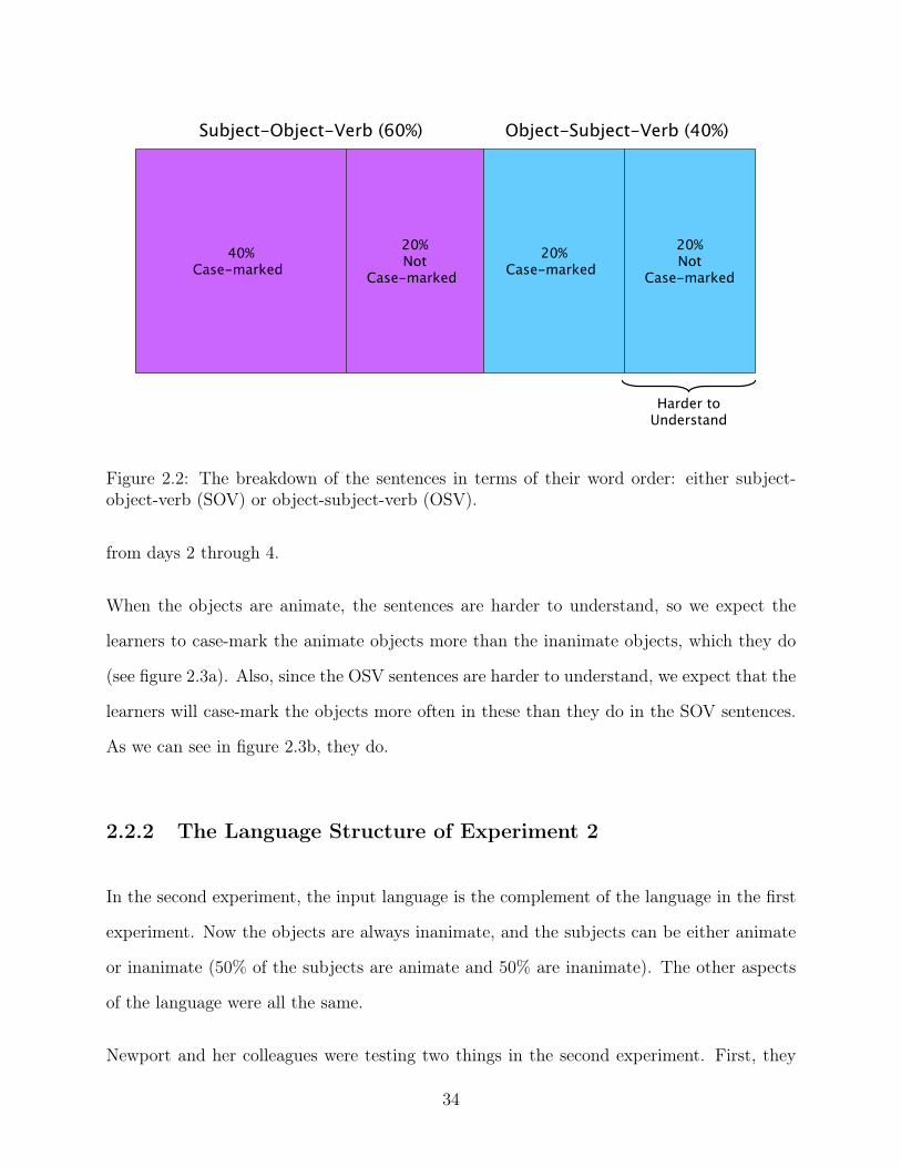
2.2 The breakdown of the sentences in terms of their word order: either subject-object-verb (SOV) or object-subject-verb (OSV). . . . . . . . . . . . . . . . 34

2.3 The results from experiment 1 in Fedzechkina et al. (2012). The black dashedline give the frequency of case marking of the source. . . . . . . . . . . . . . 35

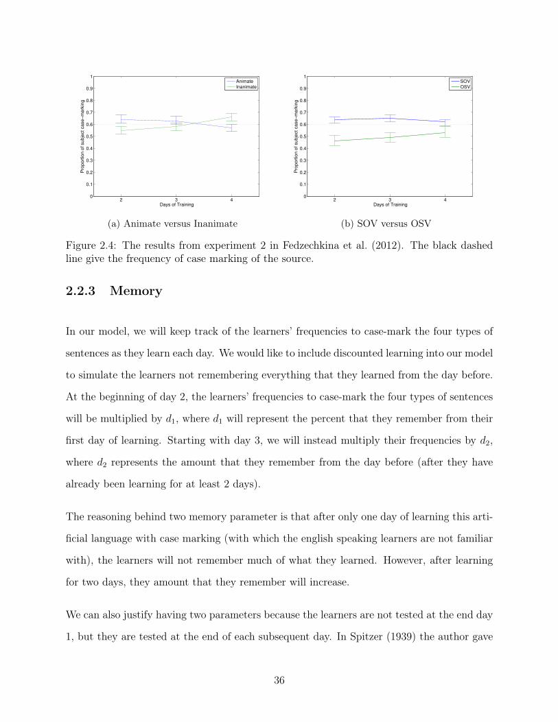
2.4 The results from experiment 2 in Fedzechkina et al. (2012). The black dashedline give the frequency of case marking of the source. . . . . . . . . . . . . . 36

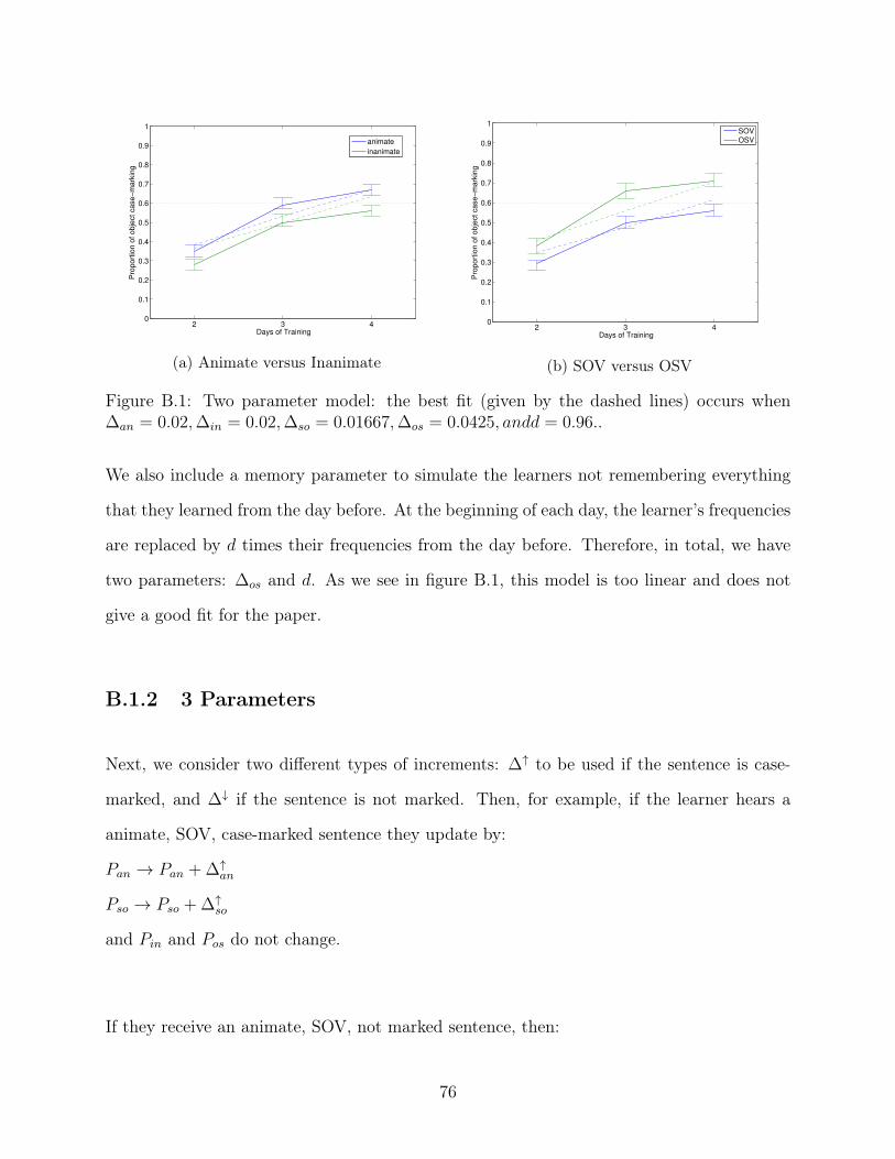
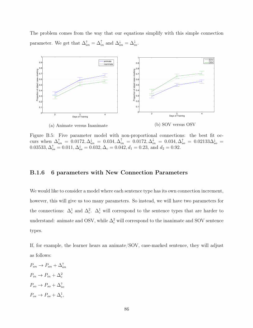
2.5 The best fit for experiment 1. It occurs when ∆+AA = 0.080,∆−AA = 0.089,∆+

UU =0.001,∆−UU = 0.017,∆+

AU = 0.0405,∆+AU = 0.0530, d1 = 0.01, and d2 = 0.97. . 40

2.6 The best fit for experiment 2. It occurs when ∆+AA = 0.013,∆−AA = 0.049,∆+

UU =0.100,∆−UU = 0.200,∆+

AU = 0.0565,∆+AU = 0.1245, d1 = 0.10, and d2 = 1.00. . 40

3.1 An example of our chosen spot (in red) and the spots within jump radius 1of it (in blue). . . . . . . . . . . . . . . . . . . . . . . . . . . . . . . . . . . . 46

3.2 An example when our our chosen spot (in red) is near the edge of the grid.The spots within jump radius 1 are in blue. . . . . . . . . . . . . . . . . . . 46

3.3 2D, 25x25, grid without talking and without mutations. . . . . . . . . . . . . 493.4 2D, 50x50, grid without talking and without mutations. . . . . . . . . . . . . 503.5 2D, 25x25, grid with talking and without mutations. . . . . . . . . . . . . . 523.6 2D, 50x50, grid with talking and without mutations. . . . . . . . . . . . . . 523.7 2D, 50x50, grid with talking and with mutation rate 0.001. . . . . . . . . . . 533.8 2D, 50x50, grid with talking and with mutation rate 0.01. . . . . . . . . . . . 533.9 1D grid without talking and without mutations. . . . . . . . . . . . . . . . . 543.10 1D grid with talking and without mutations. . . . . . . . . . . . . . . . . . . 553.11 1D grid with talking and with mutation rate 0.001. . . . . . . . . . . . . . . 55

vi

ACKNOWLEDGMENTS

First and foremost, I would like to thank my advisor, Professor Natalia Komarova, for allshe has done for me. I would also like to thank my committee members, Professor LongChen and Professor German Enciso, for their help.

Thank you to the Math department for all the help over the years.

Thank you to my friends at UCI. I have been lucky to have had wonderful officemates andfriends during my time here, and I will miss you all.

Finally, thank you to my family for all your support during this journey.

vii

CURRICULUM VITAE

Jacquelyn Leigh Rische

EDUCATION

Doctor of Philosophy in Mathematics 2014University of California, Irvine Irvine, CA

Master of Science in Mathematics 2009University of California, Irvine Irvine, CA

Bachelor of Arts in Mathematics 2007Whittier College Whittier, CA

viii

ABSTRACT OF THE DISSERTATION

Mathematical Modeling of Language Learning

By

Jacquelyn Leigh Rische

Doctor of Philosophy in Mathematics

University of California, Irvine, 2014

Professor Natalia L. Komarova, Chair

When modeling language mathematically, we can look both at how an individual learns

language, and at how language develops throughout a population. When considering indi-

vidual learning, the fascinating ability of humans to modify the linguistic input and “create”

a language has been widely discussed. In this thesis, we first look at two studies that have

investigated language learning phenomena. We create two variants of a novel learning algo-

rithm of the reinforcement-learning type which exhibits the patterns in Hudson Kam and

Newport (2009) and Fedzechkina et al. (2012), and suggests ways to explain them. Hud-

son Kam and Newport (2009) explores the differences between adults and children when it

comes to processing inconsistent linguistic input and making it more consistent. We intro-

duce an asymmetry to our algorithm that sheds light on the differences between how children

and adults regularize language. Fedzechkina et al. (2012) looks at how adults are able to

restructure their linguistic input in order to improve communication. Finally, we look at

mathematical modeling of language at the level of a population. We consider a scenario

where language is a genetic mutation that has appeared in a population without language,

and we study how language will develop in the population. We see that the language indi-

viduals have an advantage when they are able to communicate with each other and we find

conditions that enable them to “invade” the population more quickly.

ix

Introduction

The human ability to learn language is quite fascinating. As children we learn language

without formal education. We simply hear sentences from our parents and others around us.

Although the sentences we hear are not enough to recreate all the underlying grammatical

rules of our language, we, nevertheless, are able to deduce the underlying grammatical rules

and develop the same language as our parents (Komarova et al., 2001).

There are many ways to model language mathematically. For instance, it can be modeled

(i) at the level of a population, by evolutionary methods, and (ii) by focusing on the process

of individual learning. Evolutionary methods show how language emerges and develops in a

population. Using evolutionary methods, we can model how many basic features of human

language emerge (like words and grammar–see, for example, Nowak and Komarova (2001)).

We can also consider how individuals learn language. Instead of studying what is happening

in a large population, we look at how we learn as an individual, sentence by sentence, and

day by day. In this case, we focus on one specific aspect of the language, like the use

of a determiner or the concept of case marking. In particular, the fascinating ability of

humans to modify their linguistic input and “create” a language has been widely discussed.

In this thesis, we first look at two studies that have investigated such language learning

phenomena. We create a learning algorithm which exhibits the patterns reported in these

studies and suggests ways to explain them.

1

In the work of Newport and colleagues, it has been demonstrated that both children and

adults have some ability to process inconsistent linguistic input and “improve” it by making

it more consistent. In Hudson Kam and Newport (2005) and Hudson Kam and Newport

(2009), artificial miniature language acquisition from an inconsistent source was studied. It

was shown that (i) children are better at language regularization than adults, and that (ii)

adults can also regularize, depending on the structure of the input.

In Chapter 1, we create a learning algorithm of the reinforcement-learning type. We find

that in order to capture the differences between children’s and adults’ learning patterns,

we need to introduce a certain asymmetry in the learning algorithm. Namely, we have to

assume that the reaction of the learners differs depending on whether or not the source’s

input coincides with the learner’s internal hypothesis. We interpret this result in the context

of a different reaction of children and adults to positive and negative evidence. We propose

that a possible mechanism that contributes to the children’s ability to regularize an incon-

sistent input is related to their heightened sensitivity to positive evidence rather than the

(implicit) negative evidence. In our model, regularization comes naturally as a consequence

of a stronger reaction of the children to evidence supporting their preferred hypothesis. In

adults, their ability to adequately process implicit negative evidence prevents them from

regularizing the inconsistent input, resulting in a weaker degree of regularization.

Newport and colleagues have also shown that adults have the ability to restructure linguistic

input to facilitate better communication. In Fedzechkina et al. (2012), when learning an

artificial language with inefficient case marking, the learners restructure their input to make

the case marking more efficient, thus making the language easer to understand. In Chapter

2, we focus on a variant of our algorithm that models the pattens in Fedzechkina et al.

(2012). In the study, there are four sentence types, each with different degrees of ambiguity.

The meaning of an ambiguous sentence becomes clear when it is case-marked. Again, our

learning algorithm is asymmetric, and we find that the learners (who are all adults) react

2

more strongly to implicit negative feedback. Also, the learners do not remember everything

they learn. They forget a certain amount between each day of the experiment. In particular

they forget more after the first day since what they learn is not reinforced with a test at

the end of the first day (as it is at the end of each subsequent day). With these factors, the

learners are able to restructure their input and make the language more efficient.

Finally, in Chapter 3, we look at language learning on a population level. We develop and

study a model that looks at what would happen if language is a genetic mutation that

appears in a population of individuals without language. Using computer simulations, we

study how the individuals with language spread through a population of individuals without

language. We consider a population without language on one- and two-dimensional grids.

To study how the language group will grow, we focus on the effects of talking and movement.

If two individuals with language are next to each other on the grid, they can communicate.

We consider their ability to talk to be advantageous, giving them a higher reproduction rate.

Individuals are also able to move around on the grid and reproduce within a certain radius,

called the jump radius. We look at how these affect the time it takes for the individuals

with language to invade the population. We find that, for a two-dimensional grid, a jump

radius that is too small or too large will increase the time it takes to invade. However, this

phenomenon is affected by the shape of the grid. For a one-dimensional grid, we do not see

the same effect. The time to invasion decreases as the jump radius increases.

3

Chapter 1

Regularization of Languages by

Learners: A Mathematical Framework

1.1 Introduction

Natural languages evolve over time. Every generation of speakers introduces incremental

differences in their native language. Sometimes such gradual slow change gives way to an

abrupt movement when certain patterns in the language of the parents differ significantly

from those in the language of the children. The fascinating ability of humans to modify

the linguistic input and “create” a language has been widely discussed. One example is

the creation of the Nicaraguan Sign Language by children in the course of only several

years (Senghas, 1995; Senghas et al., 1997; Senghas and Coppola, 2001). Other examples

come from the creolization of pidgin languages (Andersen, 1983; Thomason and Kaufman,

1991; Sebba, 1997). It has been documented that in the time-scale of a generation, a rapid

linguistic change occurs that creates a language from something that is less than a language

(a limited pidgin language (Johnson et al., 1996), or a collection of home-signing systems in

4

the example of the Nicaraguan Sign Language).

Language regularization has been extensively studied in children, see e.g. work on the phe-

nomenon of over-regularization in children (Marcus et al., 1992). Goldin-Meadow et al.

(1984); Goldin-Meadow (2005); Coppola and Newport (2005) studied deaf children who re-

ceived no conventional linguistic input, and found that their personal communication systems

exhibited a high degree of regularity and language-like structure. The ability of adult learn-

ers to regularize has also been discussed (Klein and Perdue, 1993; Bybee and Slobin, 1982;

Cochran et al., 1999).

Much attention in the literature is paid to statistical aspects of learning, showing that learners

are able to extract a number of statistics from linguistic input with probabilistic variation

(Gómez and Gerken, 2000; Saffran, 2003; Wonnacott et al., 2008; Griffiths et al., 2010).

Identifying statistical regularities and extracting the underlying grammatical structure both

seem to contribute to human language acquisition (Seidenberg et al., 2002).

In Reali and Griffiths (2009) it was demonstrated that in the course of several generations

of learning, the speakers shift from a highly inconsistent, probabilistic language to a regular-

ized, deterministic language. A mathematical description of this phenomenon was presented

based on a Bayesian model for frequency estimation. This model demonstrated, much like

in experimental studies, that while in the course of a single “generation” no bias toward

regularization was observed, this bias became apparent after several generations. The same

phenomenon was observed in the paper Smith and Wonnacott (2010). It was suggested that

gradual, cumulative population-level processes is responsible for language regularity.

In this chapter we focus on a slightly different phenomenon. The work of Elissa Newport and

colleagues demonstrates that language regularization can also happen within one generation.

A famous example is a deaf boy Simon (see Singleton and Newport (2004)) who received all of

his linguistic input from his parents, who were not fluent in American Sign Language (ASL).

5

Simon managed to improve on this inconsistent input and master the language nearly at the

level of other children who learned ASL from a consistent source (e.g. parents, teachers, and

peers fluent in ASL). Thus he managed to surpass his parents by a large margin, suggesting

the existence of some innate tendency to regularization.

The work of Newport and her colleagues sheds light into this interesting phenomenon. In a

number of studies, it has been demonstrated that both children and adults have the ability

to process inconsistent linguistic input and “improve” it by making it more consistent. When

talking about the usage of a particular rule, this ability was termed “frequency boosting,”

as opposed to “frequency matching.” Let us suppose that the “teacher” (or the source of the

linguistic input) is inconsistent, such that it probabilistically uses several forms of a certain

rule. Frequency boosting is the ability of a language learner to increase the frequency of

usage of a particular form compared to the source. Frequency matching happens when the

learner reproduces the same frequency of usage as the source. In Hudson Kam and Newport

(2005) and Hudson Kam and Newport (2009) it was shown that (i) children are better at

frequency boosting than adults, and that (ii) adults can also frequency boost, depending on

the structure of the input.

In this chapter we create an algorithm of the reinforcement-learning type, which is capable

of reproducing the results reported in Hudson Kam and Newport (2009). It turns out that in

order to capture the differences between children’s and adults’ learning patterns, we need to

introduce a certain asymmetry in the learning algorithm. More precisely, we have to assume

that the reaction of the learners differs depending on whether or not the sources’ input

coincides with the learner’s internal hypothesis. We interpret this as learning from positive

and implicit negative evidence. We therefore propose that the differences in adults’ and

children’s abilities to regularize are related to the differences in their processing of positive

and negative evidence.

This chapter is organized as follows. In Section 1.2 we introduce the mathematical model

6

used in this paper; it belongs to a wider class of reinforcement learning models. In Section 1.3

we report the results. We describe how our model can be fitted to the data of Hudson Kam

and Newport (2009), and what parameters give rise to the observed differences between

children and adults. In Section 1.4 we summarize our findings and discuss them in terms of

processing positive and negative evidence in language acquisition.

1.2 Theory and calculations

1.2.1 Reinforcement learning in psychology and neuroscience

At the basis of our method is a mathematical model of learning which belongs to a larger

class of reinforcement-learning models (Sutton and Barto, 1998; Norman, 1972; Narendra

and Thathachar, 2012). Over the years, reinforcement models have played an important

role in modeling many aspects of cognitive and neurological processes, see e.g. Maia (2009);

Lee et al. (2012). Some of the most influential reinforcement learning algorithms have been

created by Rescorla and Wagner (1972), see also Rescorla (1968, 1988). These works have

given rise to a large number of papers in psychology and neuroscience, some of which are

reviewed in Danks (2003); Schultz (2006), see also review Miller et al. (1995) for a detailed

list of successes and failtures of the Rescorla-Wagner (RW) model.

In Schultz (2006), the neurophysiology of reward is studied. In particular, it explains that

neurons “show reward activations only when the reward occurs unpredictably and fail to

respond to well-predicted rewards, and their activity is depressed when the predicted reward

fails to occur". These arguments at the the basis of Rescorla-Wagner models, and the models

proposed below. Paper Gureckis and Love (2010) contrasts two broad classes of learning

mechanisms: one based on transformations of an internal state (e.g., recurrent network

architectures (Elman, 1990)), and the other based on learning direct associations (e.g. the

7

RW mechanism), and shows that, at least on shorter time scales, human sequence learning

appears more consistent with a process based on simple, direct associations. Models of this

kind have been used to study category learning (Love et al., 2004), learning of mathematical

concepts (Schlimm and Shultz, 2009), and visual concepts (Shultz, 2006; Baayen et al., 2011).

What is especially relevant for this work is the usage of RW type models for language learning

in humans, and even more specifically, language regularization.

Paper Ramscar and Yarlett (2007) proposes to use RW type modeling to study the process

of learning regular and irregular plural nouns. It is further shown in Ramscar et al. (2013c)

that incorporating expectation and prediction error into the model yields a surprising result

that with time, the tendency of children to over-regularize irregular plurals can be reduced

by exposing them to regular plurals.

Ramscar et al. (2013b) studied the problem of learning the meaning of words by adults

and children, and found that the informativity of objects plays a more important role for

children’s learning than for adult learning.

Ramscar et al. (2013a) studies cognitive flexibility by looking response-conflict resolution

behavior in children. The RW model is used to describe label-feature and feature-label

learning processes and predict the very different testing results by children trained by the

two methods. The success of the theory behind it is demonstrated in Ramscar et al. (2010),

where the role of negative learning and cue competition is highlighted by modeling of two

novel empirical studies. Ramscar et al. (2011) applies this theory to children’s learning of

small number words.

The theory presented below is not an attempt to explain the process of language acquisition

in its entirety (which would be a formidable task). Following a tradition in mathematical

linguistics and learning theory (see the papers cited above, as well as Steels (2000); Nowak

et al. (2001); Niyogi (2006); Lieberman et al. (2007); Hsu et al. (2013)), we have deliberately

8

simplified the task of the learner to concentrate only on certain aspects of learning. For

example, we have assumed that the learner is able to extract (segment) from all the utterances

received, the correct mutually exclusive forms 1, . . . , n of the word/rule under investigation.

This in itself is a challenge studied in the literature, see e.g. Roy and Pentland (2002);

Seidl and Johnson (2006); Monaghan et al. (2013). Once this pre-processing step has been

achieved, the learner’s task is obviously simplified.

1.2.2 The basic algorithm

Let us suppose that a certain rule has n variants (forms). A learner is characterized by a set

of n positive numbers, X = (x1, x2, . . . , xn) on a simplex:∑n

i=1 xi = 1. Each number xi is

the probability for the learner to use form i. We will call the numbers {xi} the frequencies of

the learner. If for some i = I, xI = 1, then the learner is deterministic and will consistently

use form I. The learning process is modeled as a sequence of steps, which are responses of

the learner to the input. The linguistic input (or source) emits a string of applications of the

rule, and it is characterized by a set of constant frequencies, ν1, . . . , νn (with∑n

i=1 νi = 1).

At each iteration, the learner will update its frequencies in response to the input received

from the source. If the source’s input is form j, then the learner will update its frequencies

according to the following update rules:

xk → xk − Fk(X), k 6= j, (1.1)

xj → xj +∑k 6=j

Fk(X). (1.2)

9

In this most general formulation, the function Fk can depend on any components of X. In

the case of the linear reinforcement model, we have (Narendra and Thathachar, 2012)

Fk(X) = axk, (1.3)

such that

xk → xk − axk, k 6= j, (1.4)

xj → xj + a(1− xj). (1.5)

The RW model reduces to this update rule if we assume that (1) only one stimulus is

presented at a time, and further if (2) the maximum conditioning produced by each stimulus

and the rate parameters are the same for all stimuli (the latter assumption is made for

example in Ramscar et al. (2010)).

Here we will use another version of reinforcement algorithm (1.1-1.2), whose basic form is

given by

Fk(X) =

s/(n− 1), xk > s/(n− 1),

xk, xk < s/(n− 1),(1.6)

where k 6= j, see (Mandelshtam and Komarova, 2014). Here, j is the signal emitted by

the source, and the parameter 0 < s < 1 defines the increment of a learning update. This

simple update rule states that in response to form j produced by the source, the learner

will increase its probability to use that form by a certain amount, and consequently the

probabilities of all other forms will be reduced across the board. As in the RW model, the

amount by which the strength of a certain rule is increased, depends on how “unpredictable"

10

the rule is for the current state of the learner. In RW model, the increment of learning is a

linear function of the difference between the current state xj and the maximum conditioning

(which is one). In model (1.6), it is a nonlinear function that decreases when the strength

of the rule approaches the maximum.

Learning algorithm (1.6) is a Markov process characterized by a stationary frequency dis-

tribution. That is, starting from any initial frequency vector, a learner will converge to a

quasistationary state, where the values {x1, . . . , xn} fluctuate around fixed means. Figure

1.1 demonstrates this behavior.

0 200 400 600 800 10000

0.1

0.2

0.3

0.4

0.5

0.6

0.7

0.8

0.9

1

Time Steps

Fre

quency o

f th

e L

earn

er

Form 1

Form 2

Figure 1.1: A plot of the frequency of the learner with respect to time. Here the frequencyof the learner is characterized by two forms. The frequency of the source for form 1 isν1 = .6. The increment of learning update is s = .05. Over time, the learner converges to aquasistationary state.

This algorithm possesses a source boosting property. If the (inconsistent) source is charac-

terized by a dominant usage of a certain form, on the long run the learner will use the same

form predominantly, and the frequency of usage for that form will be higher for the learner

compared to the source. Let us suppose that ν1 > 1/2 is the highest source frequency for

11

n = 2. Then at quasisteady state, the learner will use form 1 with the expected frequency

ν ′1 = 1− (1− ν1)

(s

2ν1 − 1+

1 + s

1− ν1(1 + (ν1/(1− ν1))1/s)

)> ν1, (1.7)

see Appendix A.1 for details of the calculations. Figure 1.2 demonstrates the frequency

boosting property by plotting the quasisteady state frequency ν ′1 as a function of the source

frequency, ν1. Note that the more linear reinforcement model (1.3) does not have a frequency-

boosting property, see Appendix A.2, but exhibits frequency-matching property.

0 0.2 0.4 0.6 0.8 10

0.1

0.2

0.3

0.4

0.5

0.6

0.7

0.8

0.9

1

Source Frequency: ν1

Quasis

teady S

tate

Fre

quency: ν

1’

Figure 1.2: A plot of the quasisteady state frequency ν ′1 as a function of the source frequency,ν1 (the solid line). The dashed line is the line ν ′1 = ν1. When ν1 > 1/2, we can see thefrequency boosting property (ν ′1 > ν1). For this plot, s = 0.05.

The frequency at which the dominant form is used by the source will affect the speed of

convergence of algorithm (1.6): higher frequencies lead to faster convergence. The strength

of the boosting depends on the increment of learning update, s: smaller values of s yield

larger values of ν ′. The value s also influences the speed of convergence: for higher s the

algorithm converges faster, but the frequency at which the learner uses the dominant form

decreases.

12

1.2.3 The asymmetric algorithm

The basic algorithm is characterized by a single parameter, s, which defines the increment

of learning. Next we introduce a two-parametric generalization of this algorithm, where

the update rules are different depending on whether the source’s input value matches the

highest-frequency value of the learner. Let us suppose that component xm is the largest:

xm = maxi{xi}. We define form m to be the preferred form (or the preferred hypothesis) of

the learner. Then, in responds to the source emitting form j, the update rule (1.1-1.2) will

have the following increment function:

Fk(X) =

s/(n− 1), xk > s/(n− 1), k = m,

xk, xk < s/(n− 1), k = m,

p/(n− 1), xk > p/(n− 1), k 6= m,

xk, xk < p/(n− 1), k 6= m.

(1.8)

Here is another way to express the update rules. If the source emits form j = m that matches

the largest learner’s frequency, the frequencies are updated as follows:

xk → xk − Fk, Fk =

s

n−1, xk >

sn−1

xk otherwisei 6= k

xj → xk +∑k 6=j

Fk (1.9)

13

If the source uses form j 6= m different from the learner’s preferred form, then the update is

as follows:

xk → xk − Fk, Fk =

p

n−1, xk >

pn−1

xk otherwisei 6= j

xj → xj +∑k 6=j

Fk (1.10)

If s = p, then this algorithm is the same as equation (1.6). The novel feature of the two-

parametric algorithm is that it tracks whether the source matches the learner’s “preferred”

hypothesis. If it does (that is, if the input is the form whose frequency is the largest for the

learner), then the learner increases this frequency’s value by amount defined by s. Otherwise,

the increment is defined by p (see figure 1.4). For example, in the extreme case where p� s,

the updates are only performed when the learner is reassured that its highest frequency form

is used. Otherwise the frequencies are updated very little. The two increment values, s and

p, will be refereed to as the “preferred increment” and the “non-preferred increment.”

Note that this algorithm does not simply use different reward signals on positive and negative

trials. Instead, it tracks whether the signal emitted by the source matches the current

hypothesis of the learner. For example, let us suppose that with n = 3 forms, the current

state of the learner is (0.1, 0.7, 0.2) (and we further assume that s, p < 0.05). In this case,

the preferred form of the learner is m = 2. If the source emits signal j = 1, which does not

match the preferred form, the value of x1 will receive an increment of p, and the other values

(x2 and x3) will both decrease by p/2. If the source emits signal j = 2, which matches the

preferred form, then the value of x2 will receive an increment of s, and the other values (x1

and x3) will both decrease by s/2. We can see that that depending on whether the source’s

form is the same as the preferred form of the learner, the positive increment for that form

will be different.

14

p: The Non−Preferred Increment

s: T

he P

refe

rred Incre

ment

0.1 0.2 0.3 0.4 0.5 0.6 0.7 0.8 0.9 1.0

0.1

0.2

0.3

0.4

0.5

0.6

0.7

0.8

0.9

1.0

−0.05

0

0.05

0.1

0.15

0.2

0.25

0.3

0.35

Figure 1.3: Contour plot of the value ν ′1 − ν1, which is the difference between the expectedsteady-state frequency of the learner and the frequency of the source. Here n = 2 and s andp are varied between 0.01 and 1 with step 0.01.

Figure 1.3 demonstrates the properties of the asymmetric learning algorithm depending on

the increment values, s and p, which are varied between 0.01 and 1 with step 0.01. For

the case n = 2, ν1 = 0.6, it presents the contour plot of the value ν ′1 − ν1, which is the

difference between the expected frequency of the learner at steady-state (equation (1.7)) and

the frequency of the source. All positive values correspond to the existence of the boosting

property, and the larger the value (denoted by the red colors), the stronger is the boosting

effect. We can see that the strongest boosting property is observed when the non-preferred

increment, p, is the smallest. On the other hand, the boosting effect disappears entirely if p

is significantly larger than s (the dark blue regions).

1.3 Results

In this paper we create a mathematical framework to describe adults’ and children’s learning

from an inconsistent source. We will use the results of Hudson Kam and Newport (2009) to

15

test and parametrize our model (see also Appendix A.3 for an application of our model to

the data from Hudson Kam and Newport (2005)). In Hudson Kam and Newport (2009), the

authors expose adults and children to miniature artificial languages. The participants learn

the language by listening to sentences of the language, which are presented in an inconsistent

fashion (allowing for a probabilistic usage of several forms). The structure and complexity

of the probabilistic input varies from experiment to experiment. The goal is to assess what

kinds of input are most consistent with the tendency of adults and children to regularize.

The authors also evaluate the differences in the learning patterns between adult learners and

children.

1.3.1 Regularization by adult learners

In one of the experiments performed in Hudson Kam and Newport (2009) with only adult

participants, the authors used five different types of inconsistent input. In the control case

(termed 0ND), the sentences with the “correct" (most frequent) form are given 60% of the

time, and 40% of the time sentences with an alternative form are given. In the other four

conditions, the most frequent form was also uttered 60% of the time, but different numbers

of alternative forms were used. In the 2ND case two alternative forms are each used 20%

of the time. Similarly, in each of the conditions iND with i = 2, 4, 8, 16, i alternative forms

were used (40/i)% of the time each. It was found that the adults in the control case did

not boost the frequency but rather frequency-matched the 60% of the more frequent forms.

Interestingly, as the complexity of the input increased, the learners in each of the conditions

produced the most frequent form of the language more often. That is, the frequency-boosting

increased with the number of alternative forms used.

We constructed two types of reinforcement models that describe the learning process as a

sequence of iterations. The input is a string of applications of a rule, that uses different forms

16

with certain (constant) frequencies. The learner is characterized by frequencies of usage of

each of the possible forms. After each application of the rule by the source, based on the

input, the learner updates the probabilities for each of the forms. The frequency of the

form uttered by the source increases, and all the other frequencies decrease. Figure 1.4(a)

provides a graphical illustration of this algorithm with the example of 2 alternative forms.

In the first, symmetric model, the increment is constant no matter what form is used by

the source, figure 1.4(a). In an asymmetric generalization of this model, the increments are

different depending on whether the form uttered by the source matches the most frequent

form of the learner. If the form uttered by the source is the same as the “preferred” (most

frequent) form of the learner, the corresponding frequency receives a “preferred boost,” s.

Otherwise, a “non-preferred boost” p is used. Two cases, s > p and s < p, are illustrated in

figures 1.4(b,c).

Source:

Form 1x2

x1

s>p

Source:

Form 1x2

x1

s<p

Source:

Form 1x2

x1

(a)

Source:

Form 2

Form 2

Form 1

(b)

Source:

Form 2

Form 2

Form 1

Source:

Form 2

Form 2

Form 1

(c)s=p

s

p

ss

p p

Figure 1.4: A schematic illustration of the reinforcement learning algorithm proposed here,in the case of two forms of the rule. The vertical bar represents the state of the learner: thesmall circle splits the bar into two parts, x1 and x2, with x1 + x2 = 1, such that x1 is theprobability of the learner to use form 1, and x2 is the probability of the learner to use form2. In this example, x1 > x2, that is, form 1 is the preferred form of the learner. The blackarrows show the change in the state of the learner following an utterance of the source. Ifthe source produces form 1, the value of x1 increases by amount s. If the source producesform 2, the value of x1 decreases by amount p. Three cases are presented: (a) s = p (thesymmetric learner), (b) s > p, and (c) s < p.

17

Control 2ND 4ND 8ND 16ND20%

30%

40%

50%

60%

70%

80%

90%

100%

Input Group

Me

an

Pro

du

ctio

n o

f M

ain

De

term

ine

r F

orm

s

Figure 1.5: Comparison of the results from Hudson Kam and Newport (2009) (the verticalintervals) with the results from our model (the lines), adult learners only. The dashed lineis for the best fitting symmetric reinforcement model with s = 1. The solid line is thebest-fitting asymmetric model corresponding to s = .19 and p = .50.

We performed computer simulations to study whether our models can predict the observed

patterns. For each condition, for each value of the increments s and p, we have run each

model 100 times for 1500 time steps. After each run, we noted the probability that the

learner uses the “correct" (most frequent) form by averaging its frequency found at each

time step (starting at time step 500 to give the algorithm time to converge), and averaged

these probabilities. We used these averages to calculate the least squares error compared to

the results from Hudson Kam and Newport (2009), to determine the values s and p that

best match the experimental results.

Applying the simple reinforcement model (1.6) to describe the data of Hudson Kam and

Newport (2009) we found that no parameter s gives a satisfactory fit. The best fit was

obtained for the value s = 1 and is depicted by the dashed line in figure 1.5. We can see that

this model overestimates the amount of frequency boosting compared to the experiment.

The averages that we find are (except for the 2ND group) too high when compared with the

results from the paper. Also, with s = 1 the model predicts the behavior of the learner to be

18

very unstable, characterized by frequent switchings between 0% and 100% for the frequency

of a form.

We then turned to the asymmetric model. Figure 1.6 gives a heat plot of the least square

error computed for all pairs (s, p). The dark blue areas give the best overall error. We found

that the parameters s = 0.19 and p = 0.50 give the best match. This is represented by

the solid line in figure 1.5. Therefore, for the adults, the best match comes when the “non-

preferred increment” is larger than the “preferred increment.” A similar result was obtained

when we used the data from Hudson Kam and Newport (2005), see Appendix A.3.

p: the "non−preferred increment"

s:

the

"p

refe

rre

d in

cre

me

nt"

Adults

0.1 0.2 0.3 0.4 0.5 0.6 0.7 0.8 0.9 1.0

0.1

0.2

0.3

0.4

0.5

0.6

0.7

0.8

0.9

1.0

0.1

0.2

0.3

0.4

0.5

0.6

Figure 1.6: Heat plot of least squares error of the asymmetric model compared to the resultsfrom Hudson Kam and Newport (2009). s and p vary between 0.01 and 1 with a step sizeof 0.01. The dark blue areas indicate where the smallest error occurs.

19

100% 60% + 0 ND 60% + 2 ND 60% + 4 ND0

10

20

30

40

50

60

70

80

90

100

Input Type

Mean C

orr

ect D

ete

rmin

er

Pro

duction (

%)

(a)

Child

Adult

100% 60% + 0 ND 60% + 2 ND 60% + 4 ND0

10

20

30

40

50

60

70

80

90

100

Input Group

Perc

ent S

yste

matic P

roducers

(b)

Children

Adults

Figure 1.7: Results from the experiment with children and adults in Hudson Kam andNewport (2009). (a) Correct form production. (b) Percent of systematic users broken downby children and adults for each input group.

1.3.2 Regularization by children and adults - a comparison

In order to investigate the differences in frequency boosting between children and adults,

Hudson Kam and Newport (2009) performed a similar experiment, both with children and

adult participants, by using a simpler artificial language. First, the “correct" form of the

language was used 100% of the time, and then three more conditions, 0ND, 2ND, and 4ND

were explored. Figure 1.7(a) presents the data by plotting the mean and the standard

deviation of the most frequent form production by adults and children. It was found that

children perform worse than the adults in the 100% case and similar to the adults in the

other cases.

The graphs in figure 1.7(b) contain some additional information. The authors of Hudson Kam

and Newport (2009) went a step further and measured the number of systematic users (as

opposed to “correct" users) for adults and children in each condition. Systematic users

were defined as learners that always used the same form–even if it is not the right form.

It turned out that although the number of “correct" usages (that is, usages of the most

20

frequent form of the source) in children was similar to that of the adults, the children used

their forms significantly more systematically (although their form did not always match the

most frequent form of the source). This is represented in figure 1.7(b). We can see that for

the 2 ND and 4 ND groups, the children were almost always systematic learners, while the

adults were never systematic learners.

In order to explain these data, we chose the following approach. First of all, we note that

children did not always produce the “correct" form in the 100% case. This suggests that

there was a noise factor at play here. Children did not always pay sufficient attention to the

input, which we included in the model as a noise parameter r, the probability that, although

form i was used, the child heard form j (with j 6= i). We fitted the data on the “correct"

usage (figure 1.7(a)) assuming different values of r (r = 0.2, 0.4, 0.6, and 0.8) and varying

the parameters s and p.

Figure 1.8 shows a heat-plot of the error obtained by using different values of the noise

parameter, and varying the increments. We can see that the noise level of r = 0.4 gives the

best match (it contains the most dark blue regions, which correspond to the regions with

the smallest error). However, we can see that there are two separate regions of dark blue

which correspond to two different types of learning. One is on the left side of the plot and

corresponds to very small values of p (with s > p). The other region corresponds to values

of s and p where p > s. The error estimate given by parameters from the two regions is

similar. Given the noise in the data, it is difficult to decide which parameter regime is more

consistent with reality simply on the basis of the error. Instead, we turn to the data on

systematic production.

As we know from studying the properties of the model, learners with s > p possess a larger

boosting property. This is explained graphically in figure 1.9, which assumes that there are

n = 2 forms and that form 1 is the more frequent one (ν1 > ν2 for the source). The value

of x1, the learner’s frequency for form 1, is presented by a small circle in a unit interval,

21

p

s

Children: r=0.2

20 40 60 80 100

20

40

60

80

100

p

s

Children: r=0.4

20 40 60 80 100

20

40

60

80

100

p

s

Children: r=0.6

0.2 0.4 0.6 0.8 1.0

0.2

0.4

0.6

0.8

1.0

p

s

Children: r=0.8

20 40 60 80 100

20

40

60

80

100

0.1

0.2

0.3

0.4

0.5

0.6

0.7

0.8

0.9

Figure 1.8: Error for children with four different noise rates: r = 0.2, r = 0.4, r = 0.6, andr = 0.8. For each contour plot, the values of s and p range between 0.01 and 1 with step0.01.

similar to figure 1.4. If this circle is closer to the right border of the interval, this means

that form 1 is the learner’s preferred form. Otherwise form 2 is the learner’s preferred form.

The arrows on the diagram show the direction and the relative size of the update followed

by the source’s utterance. The black arrows are the updates if the source utters form 1, and

the light green arrows are the updates if the source utters form 2.

We can see that if s > p, then the arrows pushing the dot towards the edges (zero and one)

are larger than the ones pushing it toward the middle (for s < p, this is reversed). This

means that if the learner is characterized by a stronger response to the source when the

utterance coincides with its preferred form, then the boosting tendency is observed.

22

������

������

x1

x2

x1x

1

x1

x2

x2

x2

s<ps>pForm 2 Form 2 Form 1Form 1

Form 1Form 2Form 2 Form 1

Figure 1.9: Boosting tendency occurs when s > p. The value of x1 is the learner’s frequencyfor form 1. The arrows on the diagram show the direction and the relative size of the updatefollowing the source’s utterance. The black arrows are the updates if the source utters form1, and the light green arrows are the updates if the source utters form 2.

100% 60% + 0 ND 60% + 2 ND 60% + 4 ND0

10

20

30

40

50

60

70

80

90

100

Input Type

Me

an

Co

rre

ct

De

term

ine

r P

rod

uctio

n

Child

Adult

Figure 1.10: Best fit for the children. The line gives the best fit, which corresponds tos = 1.0, p = 0.01, and r = 0.52.

From these arguments, it is clear that in order to be consistent with the data, the parameters

in the child learning model must satisfy s > p. This corresponds to the circled area in figure

1.8. Figure 1.10 presents the result of the best fit for the children. For that choice of

parameters, the learners demonstrate a large degree of consistency in their choices, even

though the choice is not always the right one. This underlies the difference between the

adult and child behavior in the experiments by Hudson Kam and Newport (2009).

23

Finally we note that for consistency, the noise parameter was also included in the fitting of

the data for the adults, see Appendix A.4. We find that the best fit for the adults occurs with

a very small noise parameter, which is consistent with the fact that the adults performed

well in the 100% case.

1.4 Discussion

In this paper we created a mathematical model of learning that is able to reproduce the

results of Hudson Kam and Newport (2009). The following summarizes our findings.

• The proposed learning algorithm is a reinforcement-type, two-parametric algorithm

(the third parameter is used to include noise). Differences in the parameters account

for the observed differences in learning patterns between adults and children. In the

algorithm, children are characterized by a stronger response to positive evidence, while

adults - by a stronger response to negative evidence.

• In our algorithm, both “adults" and “children" can demonstrate frequency-boosting be-

havior, depending on the structure of the inconsistent input. The strength of frequency

boosting increases as the number of alternative forms increases. This is consistent with

the data of Hudson Kam and Newport (2009).

• When fitted to the data, the children have a heightened ability to regularize. Most of

the child learners become “consistent users,” even if their preferred form differs from

the most frequent form of the source. Again, this is consistent with the findings of

Hudson Kam and Newport (2009).

Language regularization in children manifests itself in a number of ways, for example, children

often have difficulties learning exceptions to rules (Marcus et al., 1992). Regularization of

24

linguistic input by children has been related to overmatching or maximizing (Bever, 1982).

It has also been reported that children invent and use their own patterns (Craig and Myers,

1963).

1.4.1 Mechanisms of frequency matching and frequency boosting

The sources and mechanisms of frequency-boosting behavior have been extensively discussed

in the literature. The Language Bioprogram Hypothesis (Bickerton, 1984) has been proposed

to explain the ease with which children regularize inconsistent linguistic input when exposed

to reduced communication systems. It was argued that children utilize some innate language-

specific constraints that contribute to the process of language acquisition (DeGraff, 2001).

Overregularization in children learning grammatical rules has been explained by means of

a dual-mechanism model (Marcus, 1995), or an alternative connectionist model (Marchman

et al., 1997; Plunkett and Juola, 1999). In Wonnacott et al. (2008); Wonnacott (2011) it is

proposed that both children and adult learners use distributional statistics to make inferences

about when generalization is appropriate. The “less-is-more” hypothesis of Newport (1990)

suggests that the differences in adults’ and children’s language learning abilities can be

ascribed to children’s limited cognitive capacities. In Hudson Kam and Newport (2009), the

less-is-more hypothesis is used to explain the children’s remarkable ability to regularize.

Interestingly, the tendency of children to “maximize" has been observed in non-linguistic

contexts (see Derks and Paclisanu (1967)), where participants were asked to guess which

hand a candy is in, when the two hands contained candy at the 25:75 ratio. It was observed

that young chidren frequency boosted, and frequency matching behavior began to emerge

after the age of 4, becoing stronger in older participants. In Thompson-Schill et al. (2009);

Ramscar and Gitcho (2007) it has been suggested that, while both adults and children

have a natural tendency to regularize, the adults use their well-developed prefrontal-cortex-

25

mediated control system to override this. Adults implement their highly efficient machinery

for cognitive control and conflict processing, which has evolved for performance. In learning,

however, this may be considered an impediment as it makes regularization harder.

In this paper we explore this phenomenon further and propose an additional possible ex-

planation for the differences between adults’ and children’s abilities to generalize. This

explanation is rooted in the fundamentally different way by which adults and children deal

with negative feedback. In van Leijenhorst et al. (2006), it is suggested that while children

and adults recruit similar brain regions during risk-estimation and feedback processing, there

are some key differences between the age groups. For example, it appears that children’s

decision-making under uncertainty is associated with a high degree of response conflict, and

further, children may find negative feedback more aversive than adults do. The former fac-

tor was proposed to be responsible for the differences in learning patterns by Ramscar and

Gitcho (2007). Here we concentrate on the latter factor, the response to negative feedback,

and propose that it may be related to the observed differences in the regularization behavior

exhibited by adults and children.

By comparing simulations with data from Hudson Kam and Newport (2009), we found that

the best fitting reinforcement models were not symmetric with respect to the learning incre-

ments. That is, the increments following the source’s utterance must be different depending

on whether or not the source’s utterance coincides with the learner’s most frequent (“pre-

ferred”) form. For the child’s best fitting model, the increment following the utterance that

coincides with the learner’s most frequent form is the largest. For adults, it is the smallest.

We hypothesize that this is related to the two forms of feedback, positive and negative.

26

1.4.2 Negative feedback

The learning algorithm proposed in this paper is characterized by two parameters, s and p,

see figure 1.4. The value of s is the amount of change in the state of the learner following

the source’s input if it coincides with the learner’s present preferred hypothesis. The value

of p is the amount of change following the source’s input if it differs from the learner’s most

preferred form. Here we argue that one can regard the value s as the reaction of the learner

to positive feedback, and p as the reaction to negative feedback.

The notion of “negative evidence” or “negative feedback” is often defined as “information

about which structures are not allowed by the grammar” (Marcus, 1993; Seidenberg, 1997;

Leeman, 2003). In Chouinard and Clark (2003), negative evidence is specifically “informa-

tion that identifies children’s errors as errors during acquisition.” Most generally, negative

evidence is defined as “feedback that involves an incorrect form” (see e.g. Kang (2010), and

also in the context of second language acquisition (Doughty, 2003)). The first two definitions

are not applicable in the context of the language learning experiments of Hudson Kam and

Newport (2009). Even the latter, most general definition, cannot be used directly in the

context of learning from an inconsistent source. According to the most general definition

above, any input involving an incorrect form is negative evidence. In our setting however, the

source itself is highly probabilistic, and therefore we cannot regard the source’s utterances

of the less frequent form as “negative feedback.”

In the context of learning from an inconsistent source, it makes sense to define negative

feedback as the source’s utterances that do not coincide with the learner’s “idea”

of the correct form. A similar notion of implicit negative evidence has been proposed in the

literature, see e.g. Marcotte (2004). In Rohde and Plaut (1999) it is suggested that “ . . . one

way the statistical structure of a language can be approximated is through the formulation

and testing of implicit predictions. By comparing one’s predictions to what actually occurs,

27

feedback is immediate and negative evidence derives from incorrect predictions.” In the

illustration presented in figure 1.4, the learner’s preferred form is form 1 (because x1 > x2).

Thus negative feedback corresponds to the source’s usage of form 2.

Here we postulate that the source’s input that does not coincide with the learner’s own hy-

pothesis can be considered negative feedback. The applicability of this definition is similar

to considering “recasts" a form of negative feedback (Nicholas et al., 2001). In first language

(L1) acquisition, recasts do not occur universally, but they have been observed in Western

middle class culture, when an adult understands a child perfectly well, but chooses to re-

formulate the child’s utterance into a more adult-like form nevertheless (Tomasello, 1992).

In L1 research it has been proposed (Saxton, 1997) that this type of feedback leads to the

perception of a contrast between the original form and the adult form, which then may fa-

cilitate the child’s eventual rejection of the incorrect form. Recasts are common in second

language (L2) classroom situations. In L2 research, it has been proposed that recasts help

focus the learner’s attention on the form (as both forms convey the same meaning), and

have been considered an effective learning tool (Schmidt, 1990; Long and Robinson, 1998;

Doughty, 2001).

Although some researchers have casted doubt about the usefulness of recasts as corrective

feedback, or assumed that they simply provide positive evidence (Schwartz, 1993), much of

the literature classifies recasts as “implicit negative feedback" (Long and Robinson, 1998;

Long et al., 1998; Nicholas et al., 2001). They are thought to provide negative evidence

because they expose the gap between the learner’s form and the source’s form, by juxtaposing

target and non-target forms (Long, 2006; Adams et al., 2011). The learner compares her

own original form with the source’s input and then realizes that her language differs from

the target language. This process is called “cognitive comparison" (Nelson, 1987). The

comparison may signal that the original utterance was erroneous, thus providing the learner

with implicit negative evidence, and triggering cognitive processes that may lead to the

28

restructuring of the learner’s language (Nassaji, 2013).

1.4.3 Negative feedback in adults and children

Differences in children’s and adults’ processing of positive and negative evidence in lan-

guage acquisition have been widely discussed in the literature. It is recognized that children

preferentially utilize positive evidence while adults are relatively more successful in their

processing of negative evidence than children, see (Pinker, 1989; Birdsong, 1989; Carroll and

Swain, 1993) for language acquisition literature, and (Crone et al., 2004, 2008; Huizinga

et al., 2006) in a more general context. In the paper by Van Duijvenvoorde et al. (2008),

the authors study the neural mechanisms involved in the reaction of adults and children

to positive and negative feedback. In the experiment, the participants were shown pictures

and they had to respond whether or not the pictures followed a rule by clicking one of two

buttons. If they were correct, a plus sign was shown (to represent positive feedback) and

if they were incorrect, an “x” was shown (to represent negative feedback). The trials were

conducted in pairs. First came the “guess trial,” where the participant did not know the

rule. Next came the “repetition trial,” where the participants used the feedback from the

first trial to inform their response. The authors analyzed the participants’ MRI brain scans

obtained in the course of the experiment.

The authors looked at three different age groups: 8-9 years, 11-13 years, and 18-25 years.

Looking at the fMRI images, they found that there was activation in specific regions of the

brain. This activation was larger after negative feedback than after positive feedback for the

18-25 years old group. However, this was reversed for the young children (8-9 years old), who

had a larger activation after positive feedback. For the 11-13 years old group, the activation

amount was about the same for the positive and negative feedback. The authors concluded

that the young children had a harder time learning from negative feedback than the adults.

29

The adults were better able to process the negative feedback.

By matching our learning model with the data in Hudson Kam and Newport (2009), we

found that the best fit for the children corresponded to the learning algorithm where p was

very small and s was larger, illustrated in figure 1.4(b) (the best fit overall was for s = 1.0

and p = 0.01). This is consistent with the finding that children have a harder time processing

negative feedback. Receiving evidence that the current hypothesis is correct (which happens

when the source’s input coincides with the learner’s preferred form) evokes a strong positive

response, making the preference for that form even stronger. On the other hand, receiving

a piece of “negative” evidence (when the source’s input does not coincide with the learner’s

preferred form) is followed by a weaker response.

On the other hand, the best fit for the adults in our model occurred when s = 0.19 and

p = 0.50 (illustrated schematically in figure 1.4(c)). The adults are quick to weaken their

current hypothesis in response to the negative evidence. This is consistent with the fact that

the regions of the adult groups’ brains were activated more in reaction to negative feedback

(Van Duijvenvoorde et al., 2008).

Therefore we propose that a possible mechanism that contributes to the children’s ability to

“frequency boost” and regularize an inconsistent input is related to their heightened sensi-

tivity to positive evidence rather than the (implicit) negative evidence, in the sense defined

here. In our model, regularization comes naturally as a consequence of a stronger reaction of

the children to evidence supporting their preferred hypothesis. For adults, their ability to ad-

equately process implicit negative evidence prevents them from regularizing the inconsistent

input, resulting in a weaker degree of regularization.

30

Chapter 2

Restructuring of Languages by Learners:

A Mathematical Framework

2.1 Introduction

One way that languages get shaped is for efficient communication. In fact, many languages

have unexpected properties that make communication more efficient (see, for example, Zipf

(1949), Aylett and Turk (2004), Florian Jaeger (2010), Piantadosi et al. (2011), Qian and

Jaeger (2012), Van Son and Van Santen (2005), Piantadosi et al. (2012), Manin (2006),

andMaurits et al. (2010)). However, how these properties come about is not known.

One idea is that this shaping can happen over time, where adults might subtly change the

input for the next generation (Bates and MacWhinney (1982)). Another idea is that can also

happen as we learn, with learners changing the input they receive during language acquisition

(Florian Jaeger (2010)). In, Fedzechkina et al. (2012), Elissa Newport and colleagues look

at the later case. They consider a miniature artificial language that does not have efficient

case marking, and they want to see if the learners will make the language more efficient by

31

restructure the language as they learn it.

Consider the following two sentences: “The man the wall hit” and “The man the woman hit.”

Each sentence has a subject, an object, and a verb, but what is the subject of each sentence,

and what is the object? The meaning of the first sentence is more clear. “The man” is the

object and “the wall” is the subject. However, in the second sentence, this is not so clear.

Did the man hit the woman, or did the woman hit the man? This is an example of where

the addition of case marking would make the meaning of the sentence clear. Case marking

is the addition of marker in nouns to indicate which noun is the subject and which noun is

the object.

In Fedzechkina et al. (2012), the authors consider differential case marking systems (see,

for example, Mohanan (1994) and Aissen (2003)). In language that use differential case

marking systems, sentiences with inanimate subjects and animate objects are always case-

marked (since this combination is not typical). More typical combinations (such as animate

subjects and inanimate objects) are not marked.

2.2 Materials and Methods

2.2.1 The Language Structure of Experiment 1

In Fedzechkina et al. (2012), learners are taught an artificial language with inefficient case

marking. The artificial language consists of simple sentences with a subject, an object, and

a verb. In the first experiment, the subjects are always animate, and the objects can be

animate or inanimate. The order of the sentences can be Subject-Object-Verb (SOV) or

Object-Subject-Verb (OSV). The sentences are harder to understand when both the subject

and the object are animate. They are also harder to understand when the OSV form is used.

32

Animate Objects (50%) Inanimate Objects (50%)

Harder to Understand

30%Case-marked

20%Not

Case-marked30%

Case-marked20%Not

Case-marked

Figure 2.1: The breakdown of the sentences in terms of their object: either animate orinanimate.

The language is broken down in two ways: (i) 50% of the sentences have an animate object

and 50% of the sentences have an inanimate object, and (ii) 60% of the sentences are SOV

and 40% of the sentences are OSV. The objects are case-marked 60% of the time, with both

animate and inanimate objects being equally likely to be case-marked. Figures 2.1 and 2.2

diagram the two ways that the language is broken up.

The language has four types of sentence: (i) animate and SOV, (ii) animate and OSV, (iii)

inanimate and SOV, and (iv) inanimate and OSV. Each of these sentences will either be

case-marked or not. The way the language is presented, the case marking is not efficient.

A sentence that is harder to understand, such as an animate, OSV sentence might not

be case-marked, while an easier to understand sentence (inanimate, SOV, for example) is

case-marked.

The experiment went on for 4 days and had 20 people participating. Each day, they were

taught 80 sentences, and then tested, with the exception that they were not tested at the end

of the first day. Therefore, the paper only has data on the proportion of object case-marking

33

Subject-Object-Verb (60%) Object-Subject-Verb (40%)

Harder to Understand

40%Case-marked

20%Not

Case-marked20%

Case-marked20%Not

Case-marked

Figure 2.2: The breakdown of the sentences in terms of their word order: either subject-object-verb (SOV) or object-subject-verb (OSV).

from days 2 through 4.

When the objects are animate, the sentences are harder to understand, so we expect the

learners to case-mark the animate objects more than the inanimate objects, which they do

(see figure 2.3a). Also, since the OSV sentences are harder to understand, we expect that the

learners will case-mark the objects more often in these than they do in the SOV sentences.

As we can see in figure 2.3b, they do.

2.2.2 The Language Structure of Experiment 2

In the second experiment, the input language is the complement of the language in the first

experiment. Now the objects are always inanimate, and the subjects can be either animate

or inanimate (50% of the subjects are animate and 50% are inanimate). The other aspects

of the language were all the same.

Newport and her colleagues were testing two things in the second experiment. First, they

34

2 3 40

0.1

0.2

0.3

0.4

0.5

0.6

0.7

0.8

0.9

1

Days of Training

Pro

port

ion o

f obje

ct case−

mark

ing

animate

inanimate

(a) Animate versus Inanimate

2 3 40

0.1

0.2

0.3

0.4

0.5

0.6

0.7

0.8

0.9

1

Days of Training

Pro

port

ion o

f obje

ct case−

mark

ing

SOV

OSV

(b) SOV versus OSV

Figure 2.3: The results from experiment 1 in Fedzechkina et al. (2012). The black dashedline give the frequency of case marking of the source.

wanted to know if, in the first experiment, the preference to case-mark animate objects came

from a bias to case-mark the atypical (if this was the case, then in the second experiment,

they would expect to see the inanimate subjects being case-marked more often) or if it came

from a bias toward animate things (if this was the case, then they would expect to see the

animate sentences case-marked the most in both experiments). They found that both biases

were at play. At first, the learners case-marked animate sentences more often, but by day

three, they were case-marking the inanimate sentences more (see figure 2.4a).

With regards to the SOV and OSV sentences, the authors wanted to see if the bias was to

case-mark to avoid miscommunication (if this was the case, then we should see OSV sentences

case-marked more often again) or if it was “a bias to mention disambiguating information as

early as possible in the sentence" (if this was the case, then the SOV should be case-marked

more often). Again, they find that both biases seemed to be at play. SOV sentences are

case-marked more often than OSV, but by day 4, the rate of case-marking SOV sentences was

decreasing, while the rate of case-marking OSV sentences was increasing (see figure 2.4b).

35

2 3 40

0.1

0.2

0.3

0.4

0.5

0.6

0.7

0.8

0.9

1

Days of Training

Pro

port

ion o

f subje

ct case−

mark

ing

Animate

Inanimate

(a) Animate versus Inanimate

2 3 40

0.1

0.2

0.3

0.4

0.5

0.6

0.7

0.8

0.9

1

Days of Training

Pro

port

ion o

f subje

ct case−

mark

ing

SOV

OSV

(b) SOV versus OSV

Figure 2.4: The results from experiment 2 in Fedzechkina et al. (2012). The black dashedline give the frequency of case marking of the source.

2.2.3 Memory

In our model, we will keep track of the learners’ frequencies to case-mark the four types of

sentences as they learn each day. We would like to include discounted learning into our model

to simulate the learners not remembering everything that they learned from the day before.

At the beginning of day 2, the learners’ frequencies to case-mark the four types of sentences

will be multiplied by d1, where d1 will represent the percent that they remember from their

first day of learning. Starting with day 3, we will instead multiply their frequencies by d2,

where d2 represents the amount that they remember from the day before (after they have

already been learning for at least 2 days).

The reasoning behind two memory parameter is that after only one day of learning this arti-

ficial language with case marking (with which the english speaking learners are not familiar

with), the learners will not remember much of what they learned. However, after learning

for two days, they amount that they remember will increase.

We can also justify having two parameters because the learners are not tested at the end day

1, but they are tested at the end of each subsequent day. In Spitzer (1939) the author gave

36

reading assignments to various groups of 6th graders, and then tested their retention after

various time intervals. The students were tested on the material a total of three times over

a 63 day period. Some students were tested right after they read the article, and then again

some time later, while others were not tested right away. The students who were tested right

away did better on the subsequent tests than the other students. They found that “. . .more

is forgotten in one day without recall than is forgotten in sixty-three days with the aid of

recall.”

2.2.4 The Learning Algorithm

Suppose each individual is characterized by probabilities

Pan,so, Pan,os, Pin,so, Pin,os,

where Pan,so is the probability of the learner to case-mark an animate, SOV sentence; Pan,os is

the probability of the learner to case-mark an animate, OSV sentence; Pin,so is the probability

of the learner to case-mark an inanimate, SOV sentence; and Pin,os is the probability of the

learner to case-mark an inanimate, OSV sentence. These are numbers between 0 and 1.

In the data, these are not measured. Instead, the quantities Pan, Pin, Pso, and Pos were

presented. These are the probabilities to case-mark animate, inanimate, SOV, and OSV

sentences, respectively. Given the breakdown of the sentences (see figures 2.1 and 2.2), they

are connected with our variables as follows:

Pan = 3/5Pan,so + 2/5Pan,os, Pin = 3/5Pin,so + 2/5Pin,os, (2.1)

Pso = 1/2Pan,so + 1/2Pin,so, Pos = 1/2Pan,os + 1/2Pin,os. (2.2)

37

Note that the latter quantity is a linear combination of the first three, because

1/2Pan + 1/2Pin = 3/5Pso + 2/5Pos.

An input string can be of 8 kinds: it is characterized by a pair such as an, so, and whether

the sentence is marked or unmarked. The updates happen in the following way. Suppose a

marked an, so sentence is received. Then, we have

Pan,so →

Pan,so + ∆+an,so, Pan,so > 1/2,

Pan,so + ∆−an,so Pan,so < 1/2.

If we receive an unmarked an, so sentence, then we have

Pan,so →

Pan,so −∆−an,so, Pan,so > 1/2,

Pan,so −∆+an,so Pan,so < 1/2.

This is a variation of our model (1.9-1.10) from Chapter 1. Again, we have two different

increments that are used depending on whether or not the learner’s internal hypothesis

matches the source. For example, if the source gives a case-marked an, so sentence, and

the learner prefers to case-mark (Pan,so > 1/2), we update with the “+” increment. If the

sentence from the source does not match the learner’s hypothesis, we use the “−” increment.

(See Appendix B.1 for an alternate variation on this algorithm that also models the date

from Fedzechkina et al. (2012).)

In the simplest case, this is the only update that takes place. However, even in this simplest

case with only one sentence type updating, we have 8 variables, not including the memory

variables. To simplify, one could imagine that some of the variables are equal to each other.

The sentences in the experiment differ by the degree of ambiguity. Denoting “ambiguous"

38

by A and “unambiguous" by U, we can classify each sentence as type AA,AU,UA, or UU .

In the first experiment, animate and OSV are ambiguous, so an, so sentences are classified

as AU , as, os sentences are AA, in, so sentences are UU , and in, os sentences are UA. In

the second experiment, inanimate and OSV are ambiguous, so an, so sentences are classified

as UU , as, os sentences are UA, in, so sentences are AU , and in, os sentences are AA.

Let us consider three increment types: ∆AA,∆AU , and ∆UU (with each of they types having a

“+” and “−” increment). ∆+AA and ∆−AA will correspond to AA sentences, ∆+

AU and ∆−AU will

correspond to AU and UA sentences, and ∆+UU and ∆−UU will correspond to UU sentences.

This gives us six increment parameters and two memory parameters, for a total of eight

parameters. We can reduce the number of parameter further by assuming that

∆+AU =

∆+AA + ∆+

UU

2and ∆−AU =

∆−AA + ∆−UU2

.

This leaves us with a total of six parameters: ∆+AA,∆

−AA,∆

+UU ,∆

−UU , d1, and d2.

As in the experiments in Fedzechkina et al. (2012), we run the simulations for four days,

and the learners hear 80 sentences each day. We run the simulations for 100 learners while

varying the values of the parameters. Using least squares average, we find the parameters

that give us the best fit to the data in Fedzechkina et al. (2012).

2.3 Results

For experiment 1, the best fit occurs when ∆+AA = 0.080,∆−AA = 0.089,∆+

UU = 0.001,∆−UU =

0.017,∆+AU = 0.0405,∆+

AU = 0.0530, d1 = 0.01, and d2 = 0.97 (see figure 2.5).

For experiment 2, the best fit occurs when ∆+AA = 0.013,∆−AA = 0.049,∆+

UU = 0.100,∆−UU =

0.200,∆+AU = 0.0565,∆+

AU = 0.1245, d1 = 0.10, and d2 = 1.00 (see figure 2.6).

39

2 3 40

0.1

0.2

0.3

0.4

0.5

0.6

0.7

0.8

0.9

1

Days of Training

Pro

port

ion o

f obje

ct case−

mark

ing

animate

inanimate

(a) Animate versus Inanimate

2 3 40

0.1

0.2

0.3

0.4

0.5

0.6

0.7

0.8

0.9

1

Days of Training

Pro

port

ion o

f obje

ct case−

mark

ing

SOV

OSV

(b) SOV versus OSV

Figure 2.5: The best fit for experiment 1. It occurs when ∆+AA = 0.080,∆−AA = 0.089,∆+

UU =0.001,∆−UU = 0.017,∆+

AU = 0.0405,∆+AU = 0.0530, d1 = 0.01, and d2 = 0.97.

2 3 40

0.1

0.2

0.3

0.4

0.5

0.6

0.7

0.8

0.9

1

Days of Training

Pro

port

ion o

f subje

ct case−

mark

ing

Animate

Inanimate

(a) Animate versus Inanimate

2 3 40

0.1

0.2

0.3

0.4

0.5

0.6

0.7

0.8

0.9

1

Days of Training

Pro

port

ion o

f subje

ct case−

mark

ing

SOV

OSV

(b) SOV versus OSV

Figure 2.6: The best fit for experiment 2. It occurs when ∆+AA = 0.013,∆−AA = 0.049,∆+

UU =0.100,∆−UU = 0.200,∆+

AU = 0.0565,∆+AU = 0.1245, d1 = 0.10, and d2 = 1.00.

In both experiments, we see that the “+” increments are smaller than the “−” increments.

This agrees with our findings in Chapter 1. The adults adjust more after the inherent

negative feedback that they receive when the source’s sentence does not match their internal

hypothesis. Also in both experiments, d2 > d1, which agrees with the findings of Spitzer

(1939), who showed that we remember more of what we learn if we are tested on it right away.

We also see that in the first experiment, ∆AA > ∆UU . However, in the second experiment,

the reverse happens, and ∆UU > ∆AA.

40

2.4 Discussion

During experiment 1, Fedzechkina et al. (2012) found that the learners did restructure the

language for better communication by case-marking the ambiguous (animate and OSV)

sentences more often than the unambiguous (inanimate and SOV) sentences. Although the

sentences were broken down into animate versus inanimate and SOV versus OSV, in the

experiment each sentence was both either animate or inanimate, and either SOV or OSV.

This means that the learners could hear four types of sentences: an, so, an, os, in, so, and

in, os.

We categorized these according to their ambiguity, using A for ambiguous and U for unam-

biguous. Therefore, an, os sentences are characterized as AA, in, so sentences are character-

ized as UU , and an, so and in, os sentences are characterized as AU and UA, respectively.

With this characterization of the sentences, we have three increment types (with a “+” and

“−” increment for each type). These are ∆AA,∆AU , and ∆UU , where ∆AU =∆AA + ∆UU

2.

In our best fit for experiment 1, we found that ∆AA > ∆UU . This means that the learners

adjust more when they hear an ambiguous sentence than when they hear an unambiguous

sentence. This agrees with the finding of the experiment.

In experiment 2, we still categorize the sentences as AA,AU,UA, and UU . However, the

sentences that correspond to each of these categories is different than in the first experiment.

In the second experiment, the sentences with inanimate subjects are now the ambiguous

sentences, with OSV being ambiguous in both experiments. So now, AA corresponds to

in, os, UU corresponds to an, so, and AU/UA corresponds to in, so and an, os.

However, Fedzechkina et al. (2012) were looking a few things in the second experiment.

They wanted to know whether, in the first experiment, the learners case-marked animate

sentences more often because they were ambiguous, or because the learners had a preference

41

for animate things. If it was the former, then we would expect them to case-mark inanimate

sentences more in the second experiment (since now the inanimate sentence are ambiguous).

If it was the latter, then we would expect them to case-mark animate sentences more often

again (even though these are now unambiguous). As seen in figure 2.4a, the learner do

case-mark animate sentence more at first, but they begin to case-mark inanimate sentences

more often on day 4. In our results, we found that the best fit occurs when ∆UU > ∆AA.

This indicates that the learner’s preference towards animate sentences is stronger than their

preference to case-mark for clarity.

When comparing SOV and OSV case-marking in the second experiment, Fedzechkina et al.

(2012) were also looking at two factors. First, they were looking to see if there was a

preference towards case-marking the more ambiguous sentence (OSV), or if there was a

preference to case-mark right away. In the first experiment, the objects were case-marked

and the OSV sentences were case-marked more often. In the second experiment, the subjects

were case-marked, so they wanted to see if the SOV sentences be case-marked more often

even though they were less ambiguous. They found that the SOV sentences were indeed

case-marked more often, although by the end of day 4, it appeared that the proportion of

OSV case-marking was increasing. Again, our finding that ∆UU > ∆AA supports this. The

learner’s preference to case-mark early in the sentence is stronger than their preference to

case-mark the more ambiguous sentences.

Given the learner’s biases towards animate sentences and case-marking early in the sentence

(and thus towards SOV sentences) in the second experiment, the learners adjust more for

the unambiguous sentences. This is because, in the second experiment, the unambiguous

sentences are the sentences that they are more biased towards.

We have also seen that our asymmetric learning algorithm from Chapter 1 (model 1.9-1.10)

is versatile. We are able to use it to reproduce the results of Hudson Kam and Newport

(2005), Hudson Kam and Newport (2009) and Fedzechkina et al. (2012). We find that in all

42

the experiments, the adults’ increments are larger when their internal hypothesis does not

match the source. The adults adjust more from the inherent negative feedback they receive

in this case.

43

Chapter 3

Language as a Genetic Mutation

3.1 Introduction

We will now shift our focus to language modeled at the level of a population by evolutionary

methods. For example, Nowak and Komarova (2001) construct a mathematical framework

to develop an evolutionary theory of language. Natural selection is integrated through a

“reward” for successful communication. Using the concept of biological fitness, when indi-

viduals are able to communicate, they receive a “payoff.” This comes in the form of higher

reproductive success. Those that can communicate have a better chance at survival and will

therefore have more offspring. Evolutionary theory can show how arbitrary signals become

associated with specific referents, words are formed, syntax is developed, and grammars

evolve.

We would like to consider what happens when language first develops in a society. We will

look at a simplified case, where we have a group of individuals without language, and we

will suppose that language is a trait that appears though genetic mutation. If the offspring

of individuals without language have this mutation, they will be able to speak. We would

44

like to see how language will spread through the population, and then find conditions that

enable it to spread more quickly.

In particular, we would like to see how the ability to communicate with others will help

the individuals with language spread through the population. By being able to talk, our

individuals with language will be able to cooperate with each other. “Cooperation in hunt-

ing, making plans, coordinating activities, task sharing, social bonding, manipulation and

deception all benefit from an increase in expressive power,” (Nowak and Komarova (2001)).

3.2 Materials and Methods

We use a spatial model, where the group of individuals are set up on a grid. We look at

one- and two-dimensional grids. The one-dimensional grids consist of 625 spots in a line.

For the two-dimensional grids, we consider 25x25 grids and 50x50 grids. When we start, the

grid is randomly half filled with individuals without language. The rest of the spots on the

grid are empty. At each time step of the program, we randomly pick a spot on the grid. If

the spot is empty, we do nothing and move on to the next time step. If the spot is filled,

then the occupant has the opportunity to reproduce with probability l. They will reproduce

only if there is an empty spot near them for their offspring to go. Then they will die with

probability d. Finally, if the individual does not die, they has the opportunity to move (with

probability m) to an open spot near them (if there is an open spot).

3.2.1 Jump Radius

To define a spot to be near a given spot, we consider all the spots within a set “jump radius”

of our given spot. For a one-dimensional grid, if we look at all the spots within jump radius

r of our given spot, then we are looking at the r spots to the left and the r spots to the

45

right of our given spot (see figure 3.1a). For a two-dimensional grid, we look at the square

of spots around our given spot. If the jump radius is 1, then this is the 8 spots around our

given spot (see figure 3.1b). Jump Radius 2 gives the square of spots around jump radius

1, and so on. For both the one- and two-dimensional grids, a jump radius of infinity is the

entire grid. We consider our boundaries as being geographic barriers (see figure 3.2).

[0 0 1 1 0

](a) One-dimensional grid.

0 1 0 1 00 0 0 1 11 0 1 0 00 0 0 0 11 1 1 0 0

(b) Two-dimensional grid.

Figure 3.1: An example of our chosen spot (in red) and the spots within jump radius 1 of it(in blue).

[1 1 0 0 1

](a) One-dimensional grid.

1 1 0 1 00 0 0 1 11 0 1 0 00 0 0 0 11 1 1 0 0

(b) Two-dimensional grid.

Figure 3.2: An example when our our chosen spot (in red) is near the edge of the grid. Thespots within jump radius 1 are in blue.

We use this jump radius for both movement and reproduction. Before an individual repro-

duces or moves we consider all open spots within the given jump radius of them. We then

randomly pick one of those spots for the individual to reproduce or move to. If there are no

open spots, then the individual cannot reproduce or move.

46

3.2.2 Mutations

When an individual without language reproduces, their offspring will have a q probability

of also not having language. Therefore, there is a 1 − q probability of the offspring having

language. When q = 1, there are no mutations. When we consider cases without mutations,

in order to have individuals with language, we start with one individual with language at

the center of the grid.

3.2.3 Reproduction Rates

We have two reproduction rates in this model, l and L > l. All the individuals without

language will reproduce with the smaller rate l. When the individuals with language have

an advantage, they will reproduce with the larger rate L.

3.2.3.1 Talking

We will consider two cases. In the first case, all individuals with language will have an

advantage, and their reproduction rate will be L. We will also consider a case where the in-

dividuals with language are only advantaged if they can communicate with other individuals

with language (if there is no one near them to talk to, the ability to talk is not helpful). We

say that two individuals with language can talk when they are “near” (i.e. within jump radius

1) of each other. In this case, when an individual with language is selected to reproduce,

they will reproduce with probability l (the same as those without language) when there is

no one with language to “talk” to near them. Where there is someone to talk to, they will

reproduce with probability L > l. To study how talking will affect the spread of language,

we will compare the models with and without talking.

47

3.2.4 Time to Invasion

We define the time to invasion as the number of time steps it takes for the individuals with

language to “invade” the grid. We define “invasion” to be when the individuals without

language to die out completely. We are careful to make sure that the individuals with

language have taken over the grid (if everyone has died out, it is not an invasion).

With mutation, as long as everyone does not die out, if the individuals with language have

a higher reproduction rate, they will eventually invade. If d ≥ 0.5 or if d ≥ l, the population

will die out eventually, however, when l > 2d, the population does not die out.

The reason that language will always invade is because language individuals will keep ap-

pearing on the grid through mutation. Thus even if the language individuals die out initially,

more will appear on the grid eventually. When the individuals with language have a higher

reproduction rate, their number will eventually start to grow. Therefore, we want to look at

how the time to invasion changes as we vary the jump radius.

If we consider runs without mutations, then we start with a language individual on the grid.

It is possible for the language individuals to die out in this case (and without mutations,

they will not reappear), so if they do die out, we throw out that run and start again.

We run our simulation 1000 times, noting the time to invasion at the end of each run. We then

find the mean and standard deviation of the times to invasion. We will consider jump radius

1, 2, 3, and infinity. We would like to see how the time to invasion varies for the different

jump radii with and without talking. In all the results to follow, d = 0.2, l = 0.5, L = 0.999,

and m = 0.6.

48

3.3 Results

3.3.1 Two-Dimensional Grid without Talking

In the two-dimensional grid, without talking, we see that a larger jump radius leads to a

shorter times to invasion (see figure 3.3 for the 25x25 grid, and figure 3.4 for the 50x50

grid). This is expected, since without talking all the individuals with language have a higher

reproduction rate. Therefore, with larger jump radii, there will be more spots available to

reproduce into, and therefore more opportunity to reproduce. Therefore, they invade more

quickly.

1 2 3 Infinity4

5

6

7

8

9

10

11x 10

4 2D, Without Talking, 25x25 Grid: d=0.2, l=0.5, L=0.999, m=0.6, q=1

Tim

e t

o I

nva

sio

n

Jump Radius

Average Time to Invasion

(a) Average time to invasion, plus and minusthe standard deviation, for a 2D, 25x25, gridwithout talking and without mutations.

10.5 11 11.5 120

10

20

30

40

50

60

70

80

90

100

log(Time to Invasion)

2D, Without Talking, 25x25 Grid: d=0.2, l=0.5, L=0.999, m=0.6, q=1

Jump Radius 1

Jump Radius 2

Jump Radius 3

Jump Radius Infinity

(b) Histograms of the natural log of the timesto invasion for each jump radius.

Figure 3.3: 2D, 25x25, grid without talking and without mutations.

49

1 2 3 Infinity0.5

1

1.5

2

2.5

3

3.5

4

4.5x 10

5 2D, Without Talking, 50x50 Grid: d=0.3, l=0.5, L=0.999, m=0.6, q=1

Jump Radius

Tim

e t

o I

nva

sio

n

Average Time to Invasion

(a) Average time to invasion, plus and minusthe standard deviation, for a 2D, 50x50, gridwithout talking and without mutations.

10.5 11 11.5 12 12.5 13 13.5 140

10

20

30

40

50

60

70

80

90

1002D, Without Talking, 50x50 Grid: d=0.3, l=0.5, L=0.999, m=0.6, q=1

log(Time to Invasion)

Jump Radius 1

Jump Radius 2

Jump Radius 3

Jump Radius Infinity

(b) Histograms of the natural log of the timesto invasion for each jump radius.

Figure 3.4: 2D, 50x50, grid without talking and without mutations.

50

3.3.2 Two-Dimensional Grid with Talking

When we look at the model with talking, we expect to see a different picture. With smaller

jump radii, the offspring of individuals with language will be placed close by. Therefore, there

is more opportunity for talking to occur, and thus for the language individuals to reproduce

at the higher rate. However, with smaller jump radii, the available spots to reproduce into

will quickly fill up, leading to less reproduction. When the jump radius is too large, the

individuals with language will place their offspring farther away, so that the individuals with

language will be too far apart to talk. So although they will be able to reproduce more, they

will not be doing so with the higher rate.

We want to find the ideal jump radii such that that the offspring are not placed too far away,

but such that there are still more spots available to place their offspring. We can see this

“dip” best when we look at jump radii 1, 2, 3, and infinity. This dip is present when we do

not have mutations or when we have a very small mutation rate (see figures 3.5 and 3.6 for

q = 1, and figure 3.7 is q = .999). As the mutation rate increases, more individuals with

language appear throughout the grid due to mutation. Therefore, even when the offspring

of individuals with language are placed farther away, they are still near enough to someone

to talk to, and the dip disappears (see figure 3.8 for q = .99).

51

1 2 3 Infinity4

4.5

5

5.5

6

6.5

7

7.5

8x 10

4

Jump Radius

Tim

e t

o I

nva

sio

n

2D, With Talking, 25x25 Grid: d=0.2, l=0.5, L=0.999, m=0.6, q=1

Average Time to Invasion

(a) Average time to invasion, plus and minusthe standard deviation, for a 2D, 25x25, gridwith talking and without mutations.

10 10.2 10.4 10.6 10.8 11 11.2 11.4 11.6 11.8 120

10

20

30

40

50

60

70

80

90

100

log(Time to Invasion)

2D, With Talking, 25x25 Grid: d=0.2, l=0.5, L=0.999, m=0.6, q=1

Jump Radius Infinity

Jump Radius 1

Jump Radius 2

Jump Radius 3

(b) Histograms of the natural log of the timesto invasion for each jump radius.

Figure 3.5: 2D, 25x25, grid with talking and without mutations.

1 2 3 Infinity2

2.5

3

3.5

4

4.5

5x 10

5

Jump Radius

Tim

e t

o I

nva

sio

n

2D, With Talking, 50x50 Grid: d=0.2, l=0.5, L=0.999, m=0.6, q=1

Average Time to Invasion

(a) Average time to invasion, plus and minusthe standard deviation, for a 2D, 50x50, gridwith talking and without mutations.

12 12.2 12.4 12.6 12.8 13 13.2 13.4 13.6 13.8 140

10

20

30

40

50

60

70

80

90

100

log(Time to Invasion)

2D, With Talking, 50x50 Grid: d=0.2, l=0.5, L=0.999, m=0.6, q=1

Jump Radius Infinity

Jump Radius 1

Jump Radius 2

Jump Radius 3

(b) Histograms of the natural log of the timesto invasion for each jump radius.

Figure 3.6: 2D, 50x50, grid with talking and without mutations.

52

1 2 3 Infinity2.2

2.4

2.6

2.8

3

3.2

3.4

3.6

3.8x 10

5 2D, With Talking, 50x50 Grid: d=0.3, l=0.5, L=0.999, m=0.6, q=0.999

Jump Radius

Tim

e t

o I

nva

sio

n

Average Time to Invasion

(a) Average time to invasion, plus and minusthe standard deviation, for a 2D, 50x50, gridwith talking and with mutation rate 0.001.

12 12.5 13 13.50

10

20

30

40

50

60

70

80

90

100

log(Time to Invasion)

2D, With Talking, 50x50 Grid: d=0.3, l=0.5, L=0.999, m=0.6, q=0.999

Jump Radius Infinity

Jump Radius 1

Jump Radius 2

Jump Radius 3

(b) Histograms of the natural log of the timesto invasion for each jump radius.

Figure 3.7: 2D, 50x50, grid with talking and with mutation rate 0.001.

1 2 3 Infinity1.6

1.7

1.8

1.9

2

2.1

2.2

2.3

2.4x 10

5 2D, With Talking, 50x50 Grid: d=0.3, l=0.5, L=0.999, m=0.6, q=0.99

Jump Radius

Tim

e t

o I

nva

sio

n

Average Time to Invasion

(a) Average time to invasion, plus and minusthe standard deviation, for a 2D, 50x50, gridwith talking and with mutation rate 0.01.

11.8 11.9 12 12.1 12.2 12.3 12.4 12.5 12.6 12.7 12.80

10

20

30

40

50

60

70

80

90

100

log(Time to Invasion)

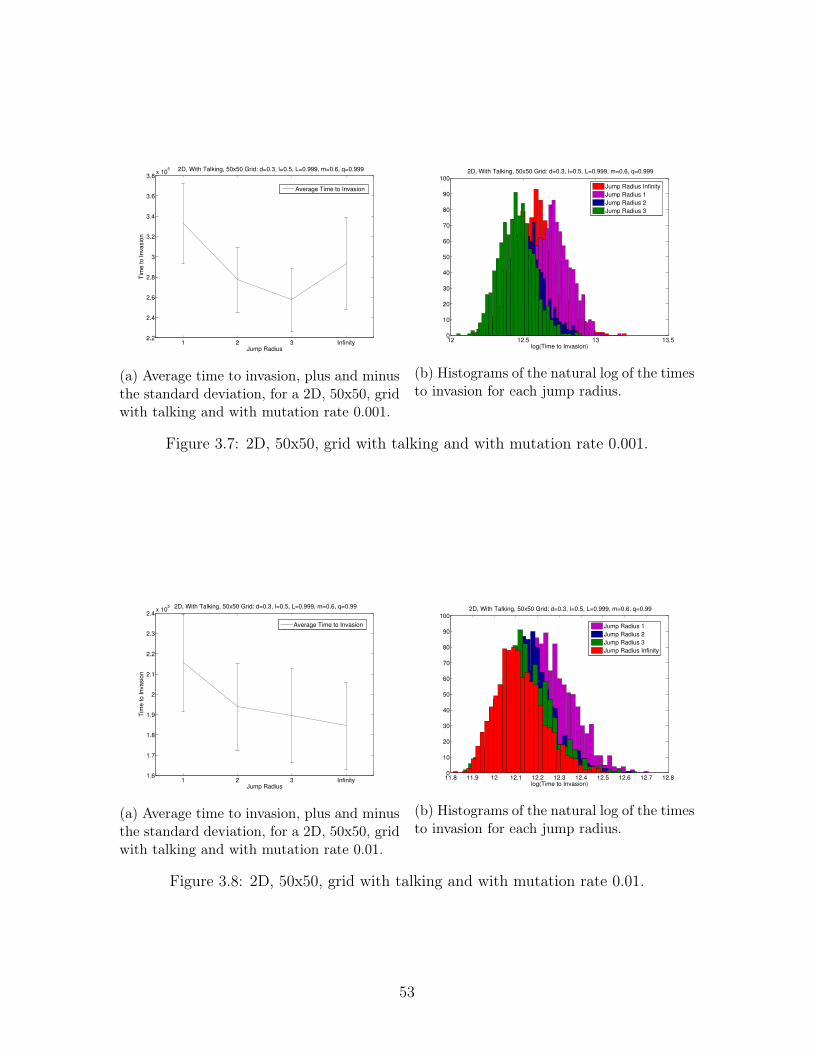
2D, With Talking, 50x50 Grid: d=0.3, l=0.5, L=0.999, m=0.6, q=0.99

Jump Radius 1

Jump Radius 2

Jump Radius 3

Jump Radius Infinity

(b) Histograms of the natural log of the timesto invasion for each jump radius.

Figure 3.8: 2D, 50x50, grid with talking and with mutation rate 0.01.

53

3.3.3 One-Dimensional Grid without Talking

In the one-dimension grid, without talking, we see that a higher jump radius leads to a

smaller time to invasion, as expected (see figure 3.9). Therefore, without talking the one-

and two-dimensional grids behave similarly.

1 2 3 Infinity0

0.5

1

1.5

2

2.5x 10

6 1D, Without Talking: d=0.2, l=0.5, L=0.999, m=0.6, q=1

Jump Radius

Tim

e t

o I

nva

sio

n

Average Time to Invasion

(a) Average time to invasion, plus and minusthe standard deviation, for a 1D grid withouttalking and without mutations.

10 10.5 11 11.5 12 12.5 13 13.5 14 14.5 150

10

20

30

40

50

60

70

80

90

1001D, Without Talking: d=0.2, l=0.5, L=0.999, m=0.6, q=1

log(Time to Invasion)

Jump Radius 1

Jump Radius 2

Jump Radius 3

Jump Radius Infinity

(b) Histograms of the natural log of the timesto invasion for each jump radius.

Figure 3.9: 1D grid without talking and without mutations.

3.3.4 One-Dimensional Grid with Talking

When we add talking to the one-dimensional grid, we can see in figure 3.10 that we do not

get the same “dip” as we do in the two-dimensional case (see figure 3.6). The overall time to

invasion does increase when we add talking, but we see that, even with talking, the time to

invasion decreases as we increase the jump radius. We get a similar graph when we add in

mutations (see figure 3.11).

54

1 2 3 Infinity0

0.5

1

1.5

2

2.5

3

3.5x 10

6 1D, With Talking: d=0.2, l=0.5, L=0.999, m=0.6, q=1

Jump Radius

Tim

e t

o I

nva

sio

n

Average Time to Invasion

(a) Average time to invasion, plus and minusthe standard deviation, for a 1D grid withtalking and without mutations.

11 11.5 12 12.5 13 13.5 14 14.5 15 15.50

10

20

30

40

50

60

70

80

901D, With Talking: d=0.2, l=0.5, L=0.999, m=0.6, q=1

log(Time to Invasion)

Jump Radius 1

Jump Radius 2

Jump Radius 3

Jump Radius Infinity

(b) Histograms of the natural log of the timesto invasion for each jump radius.

Figure 3.10: 1D grid with talking and without mutations.

1 2 3 Infinity0

1

2

3

4

5

6

7

8

9

10x 10

5

Jump Radius

Tim

e t

o I

nva

sio

n

1D, With Talking: d=0.2, l=0.5, L=0.999, m=0.6, q=0.999

Average Time to Invasion

(a) Average time to invasion, plus and minusthe standard deviation, for a 1D grid withtalking and with mutation rate 0.001.

9 10 11 12 13 14 150

20

40

60

80

100

120

1401D, With Talking: d=0.2, l=0.5, L=0.999, m=0.6, q=0.999

log(Time to Invasion)

Jump Radius 1

Jump Radius 2

Jump Radius 3

Jump Radius Infinity

(b) Histograms of the natural log of the timesto invasion for each jump radius.

Figure 3.11: 1D grid with talking and with mutation rate 0.001.

3.4 Discussion

We have seen that if we consider all the individuals with language to have an advantage,

then, the larger the jump radius, the faster the time to invasion. This makes sense, because

with a larger jump radius, there will be more reproduction, as there are more open spots

for offspring to be placed. When all the language individuals have an advantage, their

reproduction rate is larger than those without language, so they produce more offspring.

55

However, the idea that everyone with language would have an advantage is not realistic.

Language is beneficial because it allows cooperate and solve problems in parallel (see Pinker

and Bloom (1990) and Pinker (2010)). Therefore, we look at the case where the individuals

with language only have an advantage if they can talk with other individuals with language.

Thus, only the individuals with language who are able to talk to others reproduce at the

higher rate. Those who do not have anyone to talk to (as well as those without language)

reproduce at the lower rate.

We are able to see the effects of talking clearly in the two-dimensional grid. We find that we

need the jump radius to be small enough to keep those with language close enough together

so that they can talk. If the jump radius is too large, then the offspring are placed farther

away, and they do not have anyone to speak with. However, if the jump radius is too small,

then the open spots available for the offspring to be placed quickly fill, and without a place

for the offspring to go, reproduction slows. We find that the optimal jump radii are jump

radius 2 and jump radius 3. These radii are small enough that the language offspring are

kept close together so that they can talk. These radii are also large enough so that there

will be more open spots for the offspring to be placed. We find that these jump radii lead

to a faster time to invasion, both without mutations and will small mutation rates.

We do not see the same patterns in the one-dimensional grid. In these grids, even with

talking, a larger jump radius leads to a faster time to invasion. This shows a difference

between the behavior of the one- and two-dimensional grids. In the one-dimensional case,

for jump radius infinity, individuals with language appear all over the grid very quickly. This

gives the individuals with language more chances to talk to others and helps to speed up

their invasion. In the two-dimensional grid, it takes much longer for the individuals with

language to establish themselves on the grid. Once a cluster starts to develop, they will

spread quickly, but we need this cluster to appear before that will happen. This gives us an

inherent difference between the one- and two-dimensional grids.

56

Bibliography

Adams, R., NUEVO, A., and Egi, T. (2011) , The Modern Language Journal 95(s1), 42

Aissen, J. (2003) , Natural Language & Linguistic Theory 21(3), 435

Andersen, R. W. (1983) , Pidginization and Creolization as Language Acquisition., ERIC

Aylett, M. and Turk, A. (2004) , Language and Speech 47(1), 31

Baayen, R. H., Milin, P., Ðurđević, D. F., Hendrix, P., and Marelli, M. (2011) , Psychologicalreview 118(3), 438

Bates, E. and MacWhinney, B. (1982) , Language acquisition: The state of the art pp.173–218

Bever, T. G. (1982) , In Regression in mental development: Basic properties and mechanisms,pp. 153–88

Bickerton, D. (1984) , Behavioral and brain sciences 7(2), 173

Birdsong, D. (1989) , Metalinguistic performance and interlinguistic competence, Springer-Verlag Berlin

Bybee, J. L. and Slobin, D. I. (1982) , In Papers from the 5th international conference onhistorical linguistics, Vol. 21

Carroll, S. and Swain, M. (1993) , Studies in Second Language Acquisition 15(03), 357

Chouinard, M. M. and Clark, E. V. (2003) , Journal of child language 30(3), 637

Cochran, B. P., McDonald, J. L., and Parault, S. J. (1999) , Journal of Memory andLanguage 41(1), 30

Coppola, M. and Newport, E. L. (2005) , Proceedings of the National Academy of Sciencesof the United States of America 102(52), 19249

Craig, G. J. and Myers, J. L. (1963) , Child Development 34(2), 483

Crone, E. A., Richard Ridderinkhof, K., Worm, M., Somsen, R. J., and Van Der Molen,M. W. (2004) , Developmental Science 7(4), 443

57

Crone, E. A., Zanolie, K., Van Leijenhorst, L., Westenberg, P. M., and Rombouts, S. A.(2008) , Cognitive, Affective, & Behavioral Neuroscience 8(2), 165

Danks, D. (2003) , Journal of Mathematical Psychology 47(2), 109

DeGraff, M. (2001) , Language creation and language change: Creolization, diachrony, anddevelopment, The MIT Press

Derks, P. L. and Paclisanu, M. I. (1967) , Journal of Experimental Psychology 73(2), 278

Doughty, C. (2001) , Cognition and second language instruction pp. 206–257

Doughty, C. J. (2003) , The handbook of second language acquisition, Wiley-Blackwell

Elman, J. L. (1990) , Cognitive science 14(2), 179

Fedzechkina, M., Jaeger, T. F., and Newport, E. L. (2012) , PNAS 109(144), 17897

Florian Jaeger, T. (2010) , Cognitive psychology 61(1), 23

Goldin-Meadow, S. (2005) , The resilience of language: What gesture creation in deaf childrencan tell us about how all children learn language, Psychology Pr

Goldin-Meadow, S., Mylander, C., de Villiers, J., Bates, E., and Volterra, V. (1984) , Mono-graphs of the Society for Research in Child Development pp. 1–151

Gómez, R. L. and Gerken, L. (2000) , Trends in cognitive sciences 4(5), 178

Griffiths, T. L., Chater, N., Kemp, C., Perfors, A., and Tenenbaum, J. B. (2010) , Trendsin cognitive sciences 14(8), 357

Gureckis, T. M. and Love, B. C. (2010) , Cognitive science 34(1), 10

Hsu, A. S., Chater, N., and Vitányi, P. (2013) , Topics in Cognitive Science 5(1), 35

Hudson Kam, C. L. and Newport, E. L. (2005) , Language Learning and Development 1(2),151

Hudson Kam, C. L. and Newport, E. L. (2009) , Cognitive Psychology 59(1), 30

Huizinga, M. t., Dolan, C. V., and van der Molen, M. W. (2006) , Neuropsychologia 44,2017

Johnson, J. S., Shenkman, K. D., Newport, E. L., and Medin, D. L. (1996) , Journal ofMemory and Language 35(3), 335

Kang, H.-S. (2010) , The Modern Language Journal 94(4), 582

Klein, W. and Perdue, C. (1993) , In Adult language acquisition: Cross-linguistic perspectives.Volume 2. The results

Komarova, N. L., Niyogi, P., and Nowak, M. A. (2001) , J. theor. Biol. 209, 43

58

Lee, D., Seo, H., and Jung, M. W. (2012) , Annual review of neuroscience 35, 287

Leeman, J. (2003) , Studies in Second Language Acquisition 25(01), 37

Lieberman, E., Michel, J.-B., Jackson, J., Tang, T., and Nowak, M. A. (2007) , Nature449(7163), 713

Long, M. and Robinson, P. (1998) , In Focus on form in classroom second language acquisi-tion, Cambridge, UK: Cambridge University Press

Long, M. H. (2006) , Problems in SLA. Second Language Acquisition Research Series., ERIC

Long, M. H., Inagaki, S., and Ortega, L. (1998) , The modern language journal 82(3), 357

Love, B. C., Medin, D. L., and Gureckis, T. M. (2004) , Psychological review 111(2), 309

Maia, T. V. (2009) , Cognitive, Affective, & Behavioral Neuroscience 9(4), 343

Mandelshtam, Y. and Komarova, N. (2014) , arXiv preprint arXiv:1402.4678

Manin, D. (2006) , arXiv preprint cs/0612136

Marchman, V. A., Plunkett, K., and Goodman, J. (1997) , Journal of Child Language 24,767

Marcotte, J. (2004) , Journal of Linguistics pp. 1–61

Marcus, G. F. (1993) , Cognition 46(1), 53

Marcus, G. F. (1995) , Journal of Child Language 22, 447

Marcus, G. F., Pinker, S., Ullman, M., Hollander, M., Rosen, T. J., Xu, F., and Clahsen, H.(1992) , Monographs of the Society for research in child development pp. i–178

Maurits, L., Navarro, D., and Perfors, A. (2010) , In Advances in Neural InformationProcessing Systems, pp. 1585–1593

Miller, R. R., Barnet, R. C., and Grahame, N. J. (1995) , Psychological bulletin 117(3), 363

Mohanan, T. (1994) , Argument structure in Hindi, CSLI publications Stanford

Monaghan, P., White, L., and Merkx, M. M. (2013) , The Journal of the Acoustical Societyof America 134(1), EL45

Narendra, K. S. and Thathachar, M. A. (2012) , Learning automata: an introduction, CourierDover Publications

Nassaji, H. (2013) , The Grammar Dimension in Instructed Second Language Learning p.103

Nelson, K. E. (1987) , Children’s language 6, 289

59

Newport, E. L. (1990) , Cognitive Science 14(1), 11

Nicholas, H., Lightbown, P. M., and Spada, N. (2001) , Language Learning 51(4), 719

Niyogi, P. (2006) , The Computational Nature of Language Learning and Evolution, Cam-bridge: MIT Press

Norman, M. (1972) , Markov Processes and Learning Models, New York: Academic Press

Nowak, M. A. and Komarova, N. L. (2001) , TRENDS in Cognitive Sciences 5(7), 288

Nowak, M. A., Komarova, N. L., and Niyogi, P. (2001) , Science 291(5501), 114

Piantadosi, S. T., Tily, H., and Gibson, E. (2011) , Proceedings of the National Academy ofSciences 108(9), 3526

Piantadosi, S. T., Tily, H., and Gibson, E. (2012) , Cognition 122(3), 280

Pinker, S. (1989)

Pinker, S. (2010) , The language instinct: how the mind creates language, HarperCollins

Pinker, S. and Bloom, P. (1990) , Behavioral and Brain Sciences 13(4), 707

Plunkett, K. and Juola, P. (1999) , Cognitive Science 23(4), 463

Qian, T. and Jaeger, T. F. (2012) , Cognitive science 36(7), 1312

Ramscar, M., Dye, M., Gustafson, J. W., and Klein, J. (2013a) , Child development 84(4),1308

Ramscar, M., Dye, M., and Klein, J. (2013b) , Psychological science 24(6), 1017

Ramscar, M., Dye, M., and McCauley, S. M. (2013c) , Language 89(4), 760

Ramscar, M., Dye, M., Popick, H. M., and O’Donnell-McCarthy, F. (2011) , PloS one 6(7),e22501

Ramscar, M. and Gitcho, N. (2007) , Trends in cognitive sciences 11(7), 274

Ramscar, M. and Yarlett, D. (2007) , Cognitive Science 31(6), 927

Ramscar, M., Yarlett, D., Dye, M., Denny, K., and Thorpe, K. (2010) , Cognitive Science34(6), 909

Reali, F. and Griffiths, T. L. (2009) , Cognition 111(3), 317

Rescorla, R. and Wagner, A. (1972) , In Classical Conditioning II: Current Research andTheory. (A. Black and W. Prokasy eds.), New York: Appleton-Century-Crofts

Rescorla, R. A. (1968) , Journal of comparative and physiological psychology 66(1), 1

60

Rescorla, R. A. (1988) , American Psychologist 43(3), 151

Rohde, D. L. and Plaut, D. C. (1999) , Cognition 72(1), 67

Roy, D. K. and Pentland, A. P. (2002) , Cognitive Science 26(1), 113

Saffran, J. R. (2003) , Current directions in psychological science 12(4), 110

Saxton, M. (1997) , Journal of Child Language 24(01), 139

Schlimm, D. and Shultz, T. R. (2009) , In Proceedings of the 31st Annual Conference of theCognitive Science Society. Austin, TX: Cognitive Science Society, pp. 2100–5

Schmidt, R. W. (1990) , Applied linguistics 11(2), 129

Schultz, W. (2006) , Annu. Rev. Psychol. 57, 87

Schwartz, B. D. (1993) , Studies in Second Language Acquisition 15(02), 147

Sebba, M. (1997) , Contact languages: Pidgins and creoles, Macmillan London

Seidenberg, M. S. (1997) , Science 275(5306), 1599

Seidenberg, M. S., MacDonald, M. C., and Saffran, J. R. (2002) , Science 298(5593), 553

Seidl, A. and Johnson, E. K. (2006) , Developmental Science 9(6), 565

Senghas, A. (1995) , In Proceedings of the 19th Annual Boston University Conference onLanguage Development, pp. 543–552

Senghas, A. and Coppola, M. (2001) , Psychological Science 12(4), 323

Senghas, A., Coppola, M., Newport, E. L., and Supalla, T. (1997) , In Proceedings of the21st Annual Boston University Conference on Language Development, Vol. 2, pp. 550–561

Shultz, T. R. (2006) , Processes of change in brain and cognitive development: Attentionand performance 21, 61

Singleton, J. L. and Newport, E. L. (2004) , Cognitive Psychology 49(4), 370

Smith, K. and Wonnacott, E. (2010) , Cognition 116(3), 444

Spitzer, H. F. (1939) , The Journal of Educational Psyhology 30(9), 641

Steels, L. (2000) , In Parallel Problem Solving from Nature PPSN VI, pp. 17–26, Springer

Sutton, R. S. and Barto, A. G. (1998) , Reinforcement learning: An introduction, Vol. 1,Cambridge Univ Press

Thomason, S. G. and Kaufman, T. (1991) , Language contact, creolization, and geneticlinguistics, Univ of California Press

61

Thompson-Schill, S. L., Ramscar, M., and Chrysikou, E. G. (2009) , Current Directions inPsychological Science 18(5), 259

Tomasello, M. (1992) , Social development 1(1), 67

Van Duijvenvoorde, A. C., Zanolie, K., Rombouts, S. A., Raijmakers, M. E., and Crone,E. A. (2008) , The Journal of Neuroscience 28(38), 9495

van Leijenhorst, L., Crone, E. A., and Bunge, S. A. (2006) , Neuropsychologia 44(11), 2158

Van Son, R. J. and Van Santen, J. P. (2005) , Speech Communication 47(1), 100

Wonnacott, E. (2011) , Journal of Memory and Language 65(1), 1

Wonnacott, E., Newport, E. L., and Tanenhaus, M. K. (2008) , Cognitive psychology 56(3),165

Zipf, G. K. (1949)

62

Appendix A

Appendix for Chapter 1

A.1 A teacher-learner pair as a Markov walk

Consider the reinforcement learning algorithm with n = 2 forms, and suppose that the source

is characterized by the values ν1 = ν and ν2 = 1 − ν, with 0 < ν < 1. Let us describe the

reinforcement learner algorithm as a Markov walk in an interval [0, L], where the state space

consists of integer numbers in [0, L], and state i corresponse to the frequency of variant 1

being x1 = i/L. The increment of learning is denoted by ∆ and is also an integer (in this

case, increment s = ∆/L will give the increment on the interval [0, 1]). Then transition

matrix,P = {pij}, is given by the following:

pi,i+∆ = ν, for 0 ≤ i ≤ L−∆,

pi,i−∆ = 1− ν, for s ≤ i ≤ L,

pi,i+∆ = 1− ν, pL−i,L = ν for 0 ≤ i ≤ ∆− 1;

63

the rest of the entries in this matrix being zero. The stationary probability distribution is

given by the equation qP = q, where q is a string vector of probabilities. This vector has a

simple expression if the value ∆ is a divisor of L. In this case we have (for the non-normalized

eigenvector)

q =

(

1−νν

)L/∆−i, i = ks, k = 0, 1, . . . , L/∆,

0, otherwise.

The mean value for form 1 is given by

ν ′ =

∑Li=0 qii

L∑L

i=0 qi

= 1− (1− ν)

(s

2ν − 1+

1 + s

1− ν(1 + (ν/(1− ν))1/s)

).

This is a monotonically increasing function of ν with ν ′(0) = 0 and ν ′(1) = 1. We also have

the following:

ν ′(ν) < ν for ν < 1/2, ν ′(ν) > ν for ν > 1/2.

In other words, if the source uses form 1 predominantly (ν > 1/2), then the learner will be

using form 1 more often than the source, on average. The function ν ′ depends on s in the

following way. If ν < 1/2, then ∂ν ′/∂s > 0, and if ν > 1/2, then ∂ν ′/∂s < 0. In other words,

if the source uses form 1 predominantly, then increasing s will decrease the performance of

the learner.

64

A.2 The dynamical systems approach

Suppose there are only two forms, and the frequency of the source is given by ν. Let us

denote by X1 the learner’s frequency of the first form and let s be the learning increment.

The rules of the original model then can be written as follows:

If input 1 (prob. ν):

X1 → X1 + A(X1), A(X1) =

s, X1 < 1− s,

1−X1, X1 ≥ 1− s.(A.1)

If input 2 (prob. 1− ν):

X1 → X1 −B(X1), B(X1) =

s, X1 > s,

X1, X1 ≤ s.(A.2)

We would like to compare the reinforcement learning algorithm with another learning model,

the linear reward-penalty model (1.3), see also Narendra and Thathachar (2012).

For the linear reward-penalty model with two forms, we have

If input 1 (prob. ν): X1 → X1 + s(1−X1), (A.3)

If input 2 (prob. 1− ν): X1 → X1 − sX1. (A.4)

We can see that the increment of X1 is a nonlinear function of X1 in the first model, and it

is a linear function of X1 in the linear reward-penalty model. Therefore, the analysis of the

latter model is easier.

65

The mean increment in the linear reward-penalty model is given by

〈∆X1〉 = 〈νs(1−X1)− (1− ν)sX1〉 = 〈s(ν −X1)〉 = s(ν − 〈X1〉).

Therefore, at steady state, we have

〈X1〉 = ν.

For the linear reward-penalty model with n forms, we have

If input 1 (prob. ν):

X1 →

X1 + s(1−X1), max{Xj} = X1,

X1 − sX1, max{Xj} 6= X1

(A.5)

If input i (prob. 1−νn−1

):

X1 →

X1 − sX1, max{Xj} = X1,

X1 + s(

1n−1−X1

), max{Xj} 6= X1

(A.6)

where 1 < i ≤ n and 1 ≤ j ≤ n.

So if max{Xj} = X1

〈∆X1〉 =

⟨νs(1−X1)− (n− 1)

1− νn− 1

sX1

⟩= 〈s(ν −X1)〉 = s(ν − 〈X1〉).

as above in the two form case. Therefore, at steady state, we have

〈X1〉 = ν.

66

If max{Xj} 6= X1

〈∆X1〉 =

⟨ν(−sX1) + (n− 1)

1− νn− 1

s

(1

n− 1−X1

)⟩

=

⟨s

(1− vn− 1

−X1

)⟩= s

(1− νn− 1

− 〈X1〉).

Therefore, at steady state, we have

〈X1〉 =1− νn− 1

< ν

for v > 1/2 and n > 2. We conclude that the linear reward-penalty model does not possess

a frequency-boosting property.

In the original model, the above calculation does not hold because the operation of taking

the mean cannot be applied to the argument of a nonlinear function. Therefore, we have to

use the full Markov process calculation to find the mean value of X1. It is not uncommon

however to model the mean dynamics of such systems by using quasispecies equations. In

discrete time, we have

X1(t+ 1) = ν(X1 + A(X1(t))) + (1− ν)(X1 −B(X1(t))),

where the variables have the meaning of the expected values. This can also be expressed in

terms of a quasispecies-type ODE,

X1 = ν(X1 + A(X1)) + (1− ν)(X1 −B(X1))−X1.

We have three cases to consider when analyzing this equation: X1 is not near 0 or 1, X1 is

near 0, and X1 is near 1. When X1 is not near 0 or 1, the increment is given by s, so we get

67

that

X1 = (2ν − 1)s.

Therefore, when ν > 1/2, we have linear growth of X1.

When X1 is near 0, A(X1) = s and B(X1) = X1, so

X1 = (s+X1)ν −X1.

At steady state,

X1 =aν

1− ν> ν

for ν > 1− s.

When X1 is near 1, A(X1) = 1−X1 and B(X1) = s, so that

X1 = (1−X1 + s)− s.

Analyzing for steady states, we find that

X1 = 1− s(

1

ν− 1

)> ν

for ν > s.

Combining these cases together, we have a boosting property when

ν > s > 1− ν,

so

2ν > 1.

68

In other words, we see a boosting property as long as ν > 1/2. Given these conditions, at

steady state,

X1 = 1− s(

1

ν− 1

).

Note that the value obtained by this method does not coincide with the mean value obtained

by the Markov chain calculation. However, in the regime where ν is close to 1, both methods

give

X1 ≈ 1− s(1− ν).

This is because for such high frequencies, the function A(X1) is almost always linear with X1,

and the quasispecies equations describe the dynamics correctly (that is, the mean increment

is given by a linear function of the mean value of X1).

For n forms, we can see in equation (1.6) that the rules of the model are:

If input 1 (prob. ν):

X1 → X1 + A(X1), A(X1) =

s, X1 < 1− s,

1−X1, X1 ≥ 1− s.(A.7)

If input i, 1 < i ≤ n (prob. 1−νn−1

):

X1 → X −B(X1), B(X1) =

s, X1 > s,

X1, X1 ≤ s.(A.8)

69

Then in discrete time, we have

X1(t+ 1) = ν(X1 + A(X1(t))) + (n− 1)1− νn− 1

(X1 −B(X1(t)))

= ν(X1 + A(X1(t))) + (1− ν)(X1 −B(X1(t))),

where the variables have the meaning of the expected values. When we express these in

terms of an ODE, we get

X1 = ν(X1 + A(X1)) + (n− 1)1− νn− 1

(X1 −B(X1))−X1

= ν(X1 + A(X1)) + (1− ν)(X1 −B(X1))−X1

Both of these equations are the same as above, so with the same analysis, we get the for

ν > 1/2.

X = 1− s(

1

ν− 1

).

A.3 Another application of the model

In Hudson Kam and Newport (2005), Newport and her colleagues conduct experiments

similar to those from Hudson Kam and Newport (2009). In the first experiment, they create

an artificial language that is divided into two groups. The “count/mass nouns” group has the

nouns of the language divided into two classes on basis of meaning. The “gender condition”

has the nouns divided into two classes in an arbitrary fashion. Each of these is then divided

into four groups, where the determiner is used k% of the time (with k = 45 (the low group),

k = 60 (the mid group), k = 75 (the high group), and k = 100 (the perfect group)), and

70

one incorrect form is used otherwise. Altogether, there are eight groups of adults, with

five learners in each group. In this experiment, the adults were not able to regularize the

language. Their mean determiner production was almost always less than the input.

We applied model (1.9-1.10) to fit the data presented in Hudson Kam and Newport (2005).

As seen in figure A.1, for the count/mass groups, the best fit occurs when s = 0.17 and

p = 0.50. For the gender groups, the best fit occurs when s = 0.05, and p = 0.50. These

results are similar to what we found in experiment 1 from Hudson Kam and Newport (2009)

(see figure 1.5). We again find that s < p.

Low Mid High Perfect0

10

20

30

40

50

60

70

80

90

100

Input Group

Me

an

De

term

ine

r P

rod

uctio

n (

%)

Count/Mass−Paper

Gender−Paper

Input

Count/Mass−Model

Gender−Model

Figure A.1: The best fit of the model compared to the results of Hudson Kam and Newport(2005). The solid lines give the frequency of production observed in the paper (blue withcircles for the count/mass groups, and red with squares for the gender groups). The dashedlines show the best fit for each group by using model (1.9-1.10). The dashed black line givethe frequency of the input for each group. For the count/mass groups, the best fit occurswhen s = 0.17 and p = 0.50. For the gender groups, the best fit occurs when s = 0.05, andp = 0.50.

In the second experiment of Hudson Kam and Newport (2005), both children and adults were

taught a simpler artificial language. In this experiment, there were 15 children and 8 adults.

The children and adults were each divided into two groups. In one group, the determiner

was used 100% of the time. In the other, it was used 60% of the time. These groups

71

correspond to the 100% and 60% + 0ND groups in the second experiment of Hudson Kam

and Newport (2009), and their results were the same in both. The adults performed better

than the children in the 100% group, and the adults and children performed about the same

in the 60% group. However, the children were much more likely to be systematic learners.

Although it is not possible to fit these data because there are only two data points for each

group, the experimental results reported in Hudson Kam and Newport (2005) correspond to

our findings in section 1.3.2, where we modeled the second experiment of Hudson Kam and

Newport (2009).

A.4 Adding a noise parameter to the adult experiments

In figure 1.5 we found the best fit for the adults in experiment 1. Adding noise to this model

(as we did in the children’s experiment), we get a very similar best fit. With noise, the best

fit occurs when s = 0.19, p = 0.50, and r = 0.01, as shown in figure A.2.

Control 2ND 4ND 8ND 16ND20%

30%

40%

50%

60%

70%

80%

90%

100%

Input Group

Me

an

Pro

du

ctio

n o

f M

ain

De

term

ine

r F

orm

s

Figure A.2: The best fits of the model with and without noise, compared to the results ofthe paper. The solid black line gives the best fit without noise, and corresponds to s = 0.19and p = 0.50. The dashed black line gives the best fit with noise, and corresponds tos = 0.19, p = 0.50, and r = 0.01.

72

Appendix B

Appendix for Chapter 2

B.1 An Additional Variant of the Learning Algorithm

In what follows, we present another variant of our learning algorithm that is capable of

exhibiting the results from Fedzechkina et al. (2012). In the sections that follow, we will

start with a simple version of our learning algorithm, and then increase its complexity until

we are able to exhibit the patterns seen in Fedzechkina et al. (2012). With our model that

works, along with the simpler attempts that do not, we will be able to see what factors

contribute to learners restructuring the language.

B.1.1 2 Parameters

Let Pan be the learner’s frequency of the learner to case-mark an animate sentence, Pin be

the learner’s frequency of the learner to case-mark an inanimate sentence, Pso be the learner’s

frequency to case-mark a SOV sentence, and Pos be the learner’s frequency to case-mark an

OSV sentence. All the participants are native English speakers, and do not know any other

73

languages, so when we start, these frequencies will all be zero.

Given that all the sentences in the experiment are split up in two ways: animate/inanimate

(50%/50%) and SOV/OSV (60%/40%), we have the following constraint:

1

2Pan +

1

2Pin =

3

5Pso +

2

5Pos (B.1)

At each time step of the algorithm, the learner receives a sentence that is either animate or

inanimate, either SOV or OSV, and either case-marked or not (according to the probabilities

given in the paper). If the sentence is case-marked, then their frequency to case-mark will

increase by an increment. If it is not marked, then their frequency to case-mark will decrease

by an increment. The increments are given by:

∆an for animate sentences

∆in for inanimate sentences

∆so for SOV sentences

∆os for OSV sentences.

These increments also need to follow the constraint:

1

2∆an +

1

2∆in =

3

5∆so +

2

5∆os (B.2)

Let us suppose that the learner hears an animate, SOV, case-marked sentence. Then we

74

adjust as follows:

Pan → Pan + ∆an

Pso → Pso + ∆so

and Pin and Pos do not change. If they hear an animate, SOV, not marked sentence, then

we adjust as follows:

Pan → Pan −∆an

Pso → Pso −∆so

and Pin and Pos do not change.

With similar adjustments for the other types of sentences, and given (B.2), we get the

following equations:

1

2∆an =

3

5∆so

1

2∆an =

2

5∆os

1

2∆in =

3

5∆so

1

2∆in =

2

5∆os

Which we can solve to get:

∆an =4

5∆os

∆in =4

5∆os

∆so =2

3∆os

Therefore, ∆an,∆in, and ∆so all depend just on ∆os.

75

2 3 40

0.1

0.2

0.3

0.4

0.5

0.6

0.7

0.8

0.9

1

Days of Training

Pro

port

ion o

f obje

ct case−

mark

ing

animate

inanimate

(a) Animate versus Inanimate

2 3 40

0.1

0.2

0.3

0.4

0.5

0.6

0.7

0.8

0.9

1

Days of Training

Pro

port

ion o

f obje

ct case−

mark

ing

SOV

OSV

(b) SOV versus OSV

Figure B.1: Two parameter model: the best fit (given by the dashed lines) occurs when∆an = 0.02,∆in = 0.02,∆so = 0.01667,∆os = 0.0425, andd = 0.96..

We also include a memory parameter to simulate the learners not remembering everything

that they learned from the day before. At the beginning of each day, the learner’s frequencies

are replaced by d times their frequencies from the day before. Therefore, in total, we have

two parameters: ∆os and d. As we see in figure B.1, this model is too linear and does not

give a good fit for the paper.

B.1.2 3 Parameters

Next, we consider two different types of increments: ∆↑ to be used if the sentence is case-

marked, and ∆↓ if the sentence is not marked. Then, for example, if the learner hears a

animate, SOV, case-marked sentence they update by:

Pan → Pan + ∆↑an

Pso → Pso + ∆↑so

and Pin and Pos do not change.

If they receive an animate, SOV, not marked sentence, then:

76

Pan → Pan −∆↓an

Pso → Pso −∆↓so

and Pin and Pos do not change.

This gives us the following equations:

1

2∆↑an =

3

5∆↑so

1

2∆↑an =

2

5∆↑os

1

2∆↑in =

3

5∆↑so

1

2∆↑in =

2

5∆↑os

1

2∆↓an =

3

5∆↓so

1

2∆↓an =

2

5∆↓os

1

2∆↓in =

3

5∆↓so

1

2∆↓in =

2

5∆↓os

77

2 3 40

0.1

0.2

0.3

0.4

0.5

0.6

0.7

0.8

0.9

1

Days of Training

Pro

port

ion o

f obje

ct case−

mark

ing

animate

inanimate

(a) Animate versus Inanimate

2 3 40

0.1

0.2

0.3

0.4

0.5

0.6

0.7

0.8

0.9

1

Days of Training

Pro

port

ion o

f obje

ct case−

mark

ing

SOV

OSV

(b) SOV versus OSV

Figure B.2: Three parameter model: the best fit (given by the dashed lines) occurs when∆↓os, and d. The best fit occurs when ∆↑an = 0.0328,∆↓an = 0.0392,∆↑in = 0.0328,∆↓in =0.0392,∆↑so = 0.02733,∆↓so = 0.03266,∆↑os = 0.041,∆↓os = 0.049, andd = 0.91.

Which we can solve to get:

∆↑an =4

5∆↑os

∆↑in =4

5∆↑os

∆↑so =2

3∆↑os

∆↓an =4

5∆↓os

∆↓in =4

5∆↓os

∆↓so =2

3∆↓os

So we now have have three parameters: ∆↑os, ∆↓os, and d. The best fit can be seen in

figure B.2, however, it is still too linear. We do find, though, that the best fit occurs when

∆↑os < ∆↓os. This indicated that the learners are somewhat resistant to case marking, which

makes sense, given that it is a new concept to them.

78

B.1.3 4 parameters

So far, when the learner hears a sentence, we update the two sentence types contained in

that sentence, but we do nothing to the other two types. Let us consider a case where there

is a connection between the sentence types. If, for example, the learner hears an animate,

SOV, case-marked sentence, they will adjust as follows:

Pan → Pan + ∆↑an

Pin → Pin + c∆↑an

Pso → Pso + ∆↑so

Pos → Pos + c∆↑so,

and if they hear an animate, SOV, not marked sentence, they will adjust as follows:

Pan → Pan −∆↓an

Pin → Pin − c∆↓an

Pso → Pso −∆↓so

Pos → Pos − c∆↓so.

The parameter c represents how much of a connection there is between the sentence types,

and we assume that the connection amount is proportional to the amount that the main type

increased (i.e. after hearing an animate sentence, Pan increases by ∆↑an, and Pin increases by

c∆↑an).

79

With this proportional connection, our equations become:

1

2∆↑an +

1

2c∆↑in =

3

5∆↑so +

2

5c∆↑os

1

2∆↑an +

1

2c∆↑in =

3

5c∆↑so +

2

5∆↑os

1

2c∆↑an +

1

2∆↑in =

3

5∆↑so +

2

5c∆↑os

1

2c∆↑an +

1

2∆↑in =

3

5c∆↑so +

2

5∆↑os

1

2∆↓an +

1

2c∆↓in =

3

5∆↓so +

2

5c∆↓os

1

2∆↓an +

1

2c∆↓in =

3

5c∆↓so +

2

5∆↓os

1

2c∆↓an +

1

2∆↓in =

3

5∆↓so +

2

5c∆↓os

1

2c∆↓an +

1

2∆↓in =

3

5c∆↓so +

2

5∆↓os

Solving these, we get the same equations as in the 3 parameter case:

∆↑an =4

5∆↑os

∆↑in =4

5∆↑os

∆↑so =2

3∆↑os

∆↓an =4

5∆↓os

∆↓in =4

5∆↓os

∆↓so =2

3∆↓os

Now our four parameters are: ∆↑os, ∆↓os, c, and d.

80

The best fit occurs when: ∆↑os = 0.035,∆↓os = 0.042, c = 0.19, andd = 0.95 (see figure B.3).

Again, the down increments are larger than the up increments. If we consider that the

learners are all native English speakers and are not familiar with case-marking, it makes

sense that they would adjust more for the form that they are more familiar with.

2 3 40

0.1

0.2

0.3

0.4

0.5

0.6

0.7

0.8

0.9

1

Days of Training

Pro

port

ion o

f obje

ct case−

mark

ing

animate

inanimate

(a) Animate versus Inanimate

2 3 40

0.1

0.2

0.3

0.4

0.5

0.6

0.7

0.8

0.9

1

Days of TrainingP

roport

ion o

f obje

ct case−

mark

ing

SOV

OSV

(b) SOV versus OSV

Figure B.3: Four parameter model: the best fit occurs when ∆↑an = 0.028,∆↓an =0.0336,∆↑in = 0.028,∆↓in = 0.0336,∆↑so = 0.02333,∆↓so = 0.028,∆↑os = 0.035,∆↓os =0.042, c = 0.19, andd = 0.95.

B.1.4 5 Parameters

Let us consider the same model as in Section B.1.3, but with two memory parameters as

follows:

At the beginning of day 2, the learners’ frequencies to case-mark the four types of sentences

(animate, inanimate, SOV, and OSV) will be multiplied by d1, where d1 will represent the

percent that they remember from their first day of learning. Starting with day 3, we will

instead multiply their frequencies by d2, where d2 represents the amount that they remember

from the day before (after they have already been learning for at least 2 days).

The idea is that after only one day of learning this completely new, artificial language

with case marking (which the english speakers are not familiar with), the learners will not

81

remember much of what they learned. However, after learning for two days, they amount

that they remember will increase. We can also justify this change because the learners are

not tested at the end day 1, but they are tested at the end of each subsequent day. In Spitzer

(1939) the author gave reading assignments to 6th grades, and then tested their retention

after various time intervals. The students were tested on the material a total of three times

over a 63 day period. Some students were tested right after they read the article, and then

again some time later, while others were not tested right away. The students who were

tested right away did better on the subsequent tests than the other students. They found

that “. . .more is forgotten in one day without recall than is forgotten in sixty-three days

with the aid of recall.”

Our model is otherwise the same is in Section B.1.3. Recall, for example, if the learner hears

an animate/SOV, case-marked sentence, they will adjust as follows:

Pan → Pan + ∆↑an

Pin → Pin + c∆↑an

Pso → Pso + ∆↑so

Pos → Pos + c∆↑so,

and if they hear an animate/SOV, not marked sentence, they will adjust as follows:

Pan → Pan −∆↓an

Pin → Pin − c∆↓an

Pso → Pso −∆↓so

Pos → Pos − c∆↓so.

The parameter c represents how much of a connection there is.

82

So we again wind up with:

∆↑an =4

5∆↑os

∆↑in =4

5∆↑os

∆↑so =2

3∆↑os

∆↓an =4

5∆↓os

∆↓in =4

5∆↓os

∆↓so =2

3∆↓os

So now we have five parameters: ∆↑os, ∆↓os, c, d1, and d2. The best fit occurs when ∆↑os =

0.054,∆↓os = 0.065, c = 0.045, d1 = 0.11, and d2 = 0.95. We can see that in figure B.4, that

the fit is better, but we are still missing something.

2 3 40

0.1

0.2

0.3

0.4

0.5

0.6

0.7

0.8

0.9

1

Days of Training

Pro

port

ion o

f obje

ct case−

mark

ing

animate

inanimate

(a) Animate versus Inanimate

2 3 40

0.1

0.2

0.3

0.4

0.5

0.6

0.7

0.8

0.9

1

Days of Training

Pro

port

ion o

f obje

ct case−

mark

ing

SOV

OSV

(b) SOV versus OSV

Figure B.4: Five parameter model: the best fit occurs when ∆↑an = 0.0432∆↓an = 0.052,∆↑in =0.432,∆↓in = 0.052,∆↑so = 0.036,∆↓so = 0.0433,∆↑os = 0.054,∆↓os = 0.065, c = 0.045, d1 =0.11, and d2 = 0.95.

83

B.1.5 5 Parameters with Non-proportional Connections

Now let us consider a case with 5 parameters, but where the connections between the sen-

tence types is not proportional to the other type’s update as it was before. Let ∆c be the

connection increment. Then, if, for example, the learner hears an animate, SOV, case-marked

sentence, they will adjust as follows:

Pan → Pan + ∆↑an

Pin → Pin + ∆c

Pso → Pso + ∆↑so

Pos → Pos + ∆c,

and if they hear an animate, SOV, not marked sentence, they will adjust as follows:

Pan → Pan −∆↓an

Pin → Pin −∆c

Pso → Pso −∆↓so

Pos → Pos −∆c.

84

Now we get the following equations:

1

2∆↑an +

1

2∆c =

3

5∆↑so +

2

5∆c

1

2∆↑an +

1

2∆c =

3

5∆c +

2

5∆↑os

1

2∆c +

1

2∆↑in =

3

5∆↑so +

2

5∆c

1

2∆c +

1

2∆↑in =

3

5∆c +

2

5∆↑os

1

2∆↓an +

1

2∆c =

3

5∆↓so +

2

5∆c

1

2∆↓an +

1

2∆c =

3

5∆c +

2

5∆↓os

1

2∆c +

1

2∆↓in =

3

5∆↓so +

2

5∆c

1

2∆c +

1

2∆↓in =

3

5∆c +

2

5∆↓os

Solving these, we again get:

∆↑an =4

5∆↑os +

1

5∆c

∆↑in =4

5∆↑os +

1

5∆c

∆↑so =2

3∆↑os +

1

3∆c

∆↓an =4

5∆↓os +

1

5∆c

∆↓in =4

5∆↓os +

1

5∆c

∆↓so =2

3∆↓os +

1

3∆c

So now we have five parameters: ∆↑os, ∆↓os, ∆c, d1, and d2. The best fit occurs when

∆↑os = 0.011,∆↓os = 0.032,∆c = 0.042, d1 = 0.23, and d2 = 0.92, but again the fit is not great.

85

The problem comes from the way that our equations simplify with this simple connection

parameter. We get that ∆↑an = ∆↑in and ∆↓an = ∆↓in.

2 3 40

0.1

0.2

0.3

0.4

0.5

0.6

0.7

0.8

0.9

1

Days of Training

Pro

port

ion o

f obje

ct case−

mark

ing

animate

inanimate

(a) Animate versus Inanimate

2 3 40

0.1

0.2

0.3

0.4

0.5

0.6

0.7

0.8

0.9

1

Days of Training

Pro

port

ion o

f obje

ct case−

mark

ing

SOV

OSV

(b) SOV versus OSV

Figure B.5: Five parameter model with non-proportional connections: the best fit oc-curs when ∆↑an = 0.0172,∆↓an = 0.034,∆↑in = 0.0172,∆↓in = 0.034,∆↑so = 0.02133∆↓so =0.03533,∆↑os = 0.011,∆↓os = 0.032,∆c = 0.042, d1 = 0.23, and d2 = 0.92.

B.1.6 6 parameters with New Connection Parameters

We would like to consider a model where each sentence type has its own connection increment,

however, this will give us too many parameters. So instead, we will have two parameters for

the connections: ∆1c and ∆2

c . ∆1c will correspond to the sentence types that are harder to

understand: animate and OSV, while ∆2c will correspond to the inanimate and SOV sentence

types.

If, for example, the learner hears an animate/SOV, case-marked sentence, they will adjust

as follows:

Pan → Pan + ∆↑an

Pin → Pin + ∆2c

Pso → Pso + ∆↑so

Pos → Pos + ∆1c ,

86

and if they hear an animate/SOV, not marked sentence, they will adjust as follows:

Pan → Pan −∆↓an

Pin → Pin −∆2c

Pso → Pso −∆↓so

Pos → Pos −∆1c .

Or if, for example, the learner hears an inanimate/OSV, case-marked sentence, they will

adjust as follows:

Pan → Pan + ∆1c

Pin → Pin + ∆↑in

Pso → Pso + ∆2c

Pos → Pos + ∆↑os,

and if they hear an animate/SOV, not marked sentence, they will adjust as follows:

Pan → Pan −∆1c

Pin → Pin −∆↓in

Pso → Pso −∆2c

Pos → Pos −∆↓os,

So Pan and Pos both adjust by ∆1c when they are not the type that was heard, and Pin and

Pso both adjust by ∆2c when they are not the type that was heard.

87

Now we get the following equations:

1

2∆↑an +

1

2∆2c =

3

5∆↑so +

2

5∆1c

1

2∆↑an +

1

2∆2c =

3

5∆2c +

2

5∆↑os

1

2∆1c +

1

2∆↑in =

3

5∆↑so +

2

5∆1c

1

2∆1c +

1

2∆↑in =

3

5∆2c +

2

5∆↑os

1

2∆↓an +

1

2∆2c =

3

5∆↓so +

2

5∆1c

1

2∆↓an +

1

2∆2c =

3

5∆2c +

2

5∆↓os

1

2∆1c +

1

2∆↓in =

3

5∆↓so +

2

5∆1c

1

2∆1c +

1

2∆↓in =

3

5∆2c +

2

5∆↓os

Solving these, we get:

∆↑an =4

5∆↑os +

1

5∆2c

∆↑in =4

5∆↑os −∆1

c +6

5∆2c

∆↑so =2

3∆↑os −

2

3∆1c + ∆2

c

∆↓an =4

5∆↓os +

1

5∆2c

∆↓in =4

5∆↓os −∆1

c +6

5∆2c

∆↓so =2

3∆↓os −

2

3∆1c + ∆2

c

(B.3)

So we have six parameters: ∆↑os,∆↓os,∆

1c ,∆

2c , d1, and d2. The best fit occurs when: ∆↑os =

88

0.015,∆↓os = 0.032,∆1c = 0.038,∆2

c = 0.033, d1 = 0.20, and d2 = 0.88, and can be seen in

figure B.6

2 3 40

0.1

0.2

0.3

0.4

0.5

0.6

0.7

0.8

0.9

1

Days of Training

Pro

port

ion o

f obje

ct case−

mark

ing

animate

inanimate

(a) Animate versus Inanimate

2 3 40

0.1

0.2

0.3

0.4

0.5

0.6

0.7

0.8

0.9

1

Days of Training

Pro

port

ion o

f obje

ct case−

mark

ing

SOV

OSV

(b) SOV versus OSV

Figure B.6: Six parameter model: the best fit occurs when: ∆↑an = 0.0186,∆↓an =0.0322,∆↑in = 0.0136,∆↓in = 0.0272,∆↑so = 0.017667,∆↓so = 0.0290,∆↑os = 0.015,∆↓os =0.032,∆1

c = 0.038,∆2c = 0.033, d1 = 0.20, and d2 = 0.88.

B.1.7 Experiment 2

Using the same model as in section B.1.6, and assuming that the memory parameters should

be near what they were in experiment 1 we get the that the best fit occurs when: ∆↑os =

0.14,∆↓os = 0.211,∆1c = 0.005,∆2

c = 0.630, d1 = 0.17, and d2 = 0.87 (see figure B.7).

B.2 Discussion

We find that our six parameter model in B.1.6 is able to exhibit the patterns seen in both

the experiments in Fedzechkina et al. (2012). We need different increments for when the

sentences were case-marked, then for when they are not marked. We also need two connection

parameters, and 2 memory parameters.

89

2 3 40

0.1

0.2

0.3

0.4

0.5

0.6

0.7

0.8

0.9

1

Days of Training

Pro

port

ion o

f subje

ct case−

mark

ing

Animate

Inanimate

(a) Animate versus Inanimate

2 3 40

0.1

0.2

0.3

0.4

0.5

0.6

0.7

0.8

0.9

1

Days of Training

Pro

port

ion o

f subje

ct case−

mark

ing

SOV

OSV

(b) SOV versus OSV

Figure B.7: The best fit occurs when: ∆↑an = 0.238,∆↓an = 0.2948,∆↑in = 0.863,∆↓in =0.9198,∆↑so = 0.72,∆↓so = 0.76733,∆↑os = 0.14,∆↓os = 0.211,∆1

c = 0.005,∆2c = 0.630, d1 =

0.17, and d2 = 0.87.

We find that “up” parameters that correspond to case marking are smaller than the “down”

parameters. This indicates that the learners are somewhat resistant to case marking, and

react more strongly when they hear a sentence that is not marked. We also find that the

connection parameter that corresponds to the harder to understand sentences is larger than

the other connection parameter. This indicates that the learners adjust their frequencies

more for the more difficult sentences. Finally, our memory parameter for the beginning

of day 2 is much smaller than the memory parameter for the subsequent parameters. We

attribute this to the fact that the learners are not tested at the end of day 1, and therefore,

do not remember much about what they learned from that day. Once they start getting

tested at the end of each day, they are able to retain more of what they learn.

90