274
Mathematical Modeling of Transport Phenomena in Polymer Electrolyte and Direct Methanol Fuel Cells Doctoral Thesis Stockholm, Sweden 2004 ERIK BIRGERSSON

TRITA-MEKTechnical Report 2004:02
ISSN 0348-467XISRN KTH/MEK/TR—04/02—SE
www.kth.se
ERIK BIRG
ERSSON
Mathem
atical Modeling of TransportPhenom
ena in Polymer Electrolyte and D
irectMethanol Fuel Cells
Mathematical Modeling ofTransport Phenomena in
Polymer Electrolyte and Direct Methanol Fuel Cells
Doctoral ThesisStockholm, Sweden 2004
E R I K B I R G E R S S O N
KTH 20
04


Mathematical Modeling of Transport Phenomena inPolymer Electrolyte and Direct Methanol Fuel Cells
by
Erik Birgersson
February 2004Technical Reports from
Royal Institute of TechnologyDepartment of MechanicsS-100 44 Stockholm, Sweden

Typsatt i AMS-LATEX.
Akademisk avhandling som med tillstånd av Kungliga Tekniska Högskolan iStockholm framlägges till offentlig granskning för avläggande av teknologiedoktorsexamen den 4 Februari 2004 kl 10.15 i Kollegiesalen, Administrations-byggnaden, Kungliga Tekniska Högskolan, Valhallavägen 79, Stockholm.
c°Erik Birgersson 2004Universitetsservice US-AB, Stockholm 2004

Mathematical Modeling of Transport Phenomena in PolymerElectrolyte and Direct Methanol Fuel Cells
Erik BirgerssonDepartment of Mechanics, Royal Institute of TechnologySE-100 44 Stockholm, Sweden.
AbstractThis thesis deals with modeling of two types of fuel cells: the polymer elec-trolyte fuel cell (PEFC) and the direct methanol fuel cell (DMFC), for which weaddress four major issues: a) mass transport limitations; b) water management(PEFC); c) gas management (DMFC); d) thermal management.
Four models have been derived and studied for the PEFC, focusing on thecathode. The first exploits the slenderness of the cathode for a two-dimensionalgeometry, leading to a reduced model, where several nondimensional parame-ters capture the behavior of the cathode. The model was extended to threedimensions, where four different flow distributors were studied for the cathode.A quantitative comparison shows that the interdigitated channels can sustainthe highest current densities. These two models, comprising isothermal gas-phase flow, limit the studies to (a). Returning to a two-dimensional geometry ofthe PEFC, the liquid phase was introduced via a separate flow model approachfor the cathode. In addition to conservation of mass, momentum and species,the model was extended to consider simultaneous charge and heat transfer forthe whole cell. Different thermal, flow fields, and hydrodynamic conditionswere studied, addressing (a), (b) and (d). A scale analysis allowed for pre-dictions of the cell performance prior to any computations. Good agreementbetween experiments with a segmented cell and the model was obtained.
A liquid-phase model, comprising conservation of mass, momentum andspecies, was derived and analyzed for the anode of the DMFC. The impact ofhydrodynamic, electrochemical and geometrical features on the fuel cell per-formance were studied, mainly focusing on (a). The slenderness of the anodeallows the use of a narrow-gap approximation, leading to a reduced model, withbenefits such as reduced computational cost and understanding of the physi-cal trends prior to any numerical computations. Adding the gas-phase via amultiphase mixture approach, the gas management (c) could also be studied.Experiments with a cell, equipped with a transparent end plate, allowed forvisualization of the flow in the anode, as well as validation of the two-phasemodel. Good agreement between experiments and the model was achieved.
Descriptors: Fuel cell; DMFC; PEFC; one-phase; two-phase; model; visualcell; segmented cell; scale analysis; asymptotic analysis.
Preface
This thesis considers modelling of transport phenomena in polymer elec-trolyte and direct methanol fuel cells. The thesis is based on the followingpapers:
Paper 1. Vynnycky, M. and Birgersson, E. 2002, ‘Analysis of a Model ForMulticomponent Mass Transfer in the Cathode of a Polymer Electrolyte FuelCell’. SIAM (Soc. Ind. Appl. Math.) Journal of Applied Mathematics, 63,1392-1423 (2003).
Paper 2. Birgersson, E. and Vynnycky, M. 2002, ‘A Quantitative Study of theEffect of Flow-Distributor Geometry in the Cathode of a PEFC’. Manuscript.
Paper 3. Birgersson, E., Noponen, M., and Vynnycky, M., ‘Analysis of aTwo-phase Non-Isothermal Model for a PEFC’. Manuscript.
Paper 4. Noponen, M., Birgersson, E., Ihonen, J., Vynnycky, M., Lundblad,A. and Lindbergh, G., ‘A Two-Phase Non-Isothermal PEFC Model: Theoryand Validation’. Submitted to Fuel Cells - From Fundamentals to Systems(2003).
Paper 5. Birgersson, E., Nordlund, J., Ekström, H., Vynnycky, M. and Lind-bergh, G., ‘Reduced Two-Dimensional One-Phase Model for Analysis of theAnode of a DMFC’. Journal of the Electrochemical Society, 150, A1368-A1376(2003).
Paper 6. Nordlund, J., Picard, C., Birgersson, E., Vynnycky, M. and Lind-bergh, G., ‘The Design and Usage of a Visual Direct Methanol Fuel Cell’.Submitted to Journal of Applied Electrochemistry (2003).
Paper 7. Birgersson, E., Nordlund, J., Vynnycky, M., Picard, C. and Lind-bergh, G., ‘Reduced Two-Phase Model for Analysis of the Anode of a DMFC’.To be submitted to Journal of the Electrochemical Society.
The papers are re-set in the present thesis format.
iv

PREFACE v
Division of work between authors
Paper 1: The problem formulation was performed jointly by the authors. Theanalysis, coding and numerical simulations were performed by M. Vynnycky(MV). Post-processing of data was performed by MV and E. Birgersson (EB).The report was written mainly by MV, with feedback from EB.
Paper 2: The problem formulation, coding, numerical simulations and post-processing were performed by EB. The report was written mainly by EB, withfeedback from MV.
Paper 3: The problem formulation for the mathematical model, coding, nu-merical simulations and post-processing were performed in close cooperationbetween M. Noponen (MN) and EB. EB performed the analysis with feedbackfrom MV. The report was written by EB and MN, with feedback from MV.
Paper 4: The problem formulation for the mathematical model, coding, nu-merical simulations and post-processing were performed in close cooperationbetween MN and EB. The experiments were carried out by MN and J. Ihonen(JI). The report was written by EB and MN, with feedback from MV.
Paper 5: The problem formulation, analysis, coding, numerical simulationsand post-processing were performed by EB with feedback from MV. J. Nord-lund (JN) provided the electrokinetics and the main part of the constitutiverelations and parameters. The report was written in close cooperation betweenEB and JN, with feedback from MV and G. Lindbergh (GL).
Paper 6: The problem formulation was performed mainly by JN, with somefeedback from EB. The cell was designed by JN and the peripheral equipmentset up by JN and Cyril Picard (CP). The experiments and post-processing werecarried out by CP under supervision of JN for the electrochemical part and EBfor the hydrodynamic part. The report was written by JN, with feedback fromEB, CP, GL and MV.
Paper 7: The problem formulation, analysis and coding were performed byEB with feedback from MV. JN provided the electrokinetics, equilibrium con-ditions and the main part of the constitutive relations and parameters. Theexperiments were carried out by CP under supervision of JN for the electro-chemical part and EB for the hydrodynamic part. Numerical simulations andpost-processing were performed by EB and JN. The report was written in closecooperation between EB and JN, with feedback from MV.

Contents
Preface iv
Chapter 1. Introduction 8
Chapter 2. Fuel cells 101. Basic principles 102. Overview of fuel cell technologies 123. Polymer electrolyte and direct methanol fuel cells 13
Chapter 3. Basic concepts 171. Volume averaging 172. Governing equations 183. Electrokinetics and the active layers 234. Scale analysis and nondimensional numbers 255. Numerical tools and methodologies 27
Chapter 4. Summary of results 281. Polymer electrolyte fuel cells 282. Direct methanol fuel cells 33
Chapter 5. Discussion and Outlook 38
Acknowledgments 40
Bibliography 41
Paper 1: Analysis of a Model For Multicomponent Mass Transfer in theCathode of a Polymer Electrolyte Fuel Cell
Paper 2: A Quantitative Study of the Effect of Flow-Distributor Geometryin the Cathode of a PEM Fuel Cell
Paper 3: Analysis of a Two-phase Non-Isothermal Model for a PEFC
Paper 4: A Two-Phase Non-Isothermal PEFC Model: Theory andValidation
Paper 5: Reduced Two-Dimensional One-Phase Model for Analysis of theAnode of a DMFC
vi

CONTENTS vii
Paper 6: The Design and Usage of a Visual Direct Methanol Fuel Cell
Paper 7: Reduced Two-Phase Model for Analysis of the Anode of a DMFC

CHAPTER 1
Introduction
In view of ever increasing levels of environmental pollution and thus adesire to replace the fossil-fuel-based economy with a cleaner alternative, thefuel cell has in recent years emerged as a prime candidate for automotive,portable and stationary applications. These fuel cells convert hydrogen orhydrocarbon fuels directly into electricity. High efficiency, as the fuel cell isnot limited by the Carnot-efficiency, low emissions, silent operation, no movingparts and a scalable system, number among the main advantages of fuel cells.
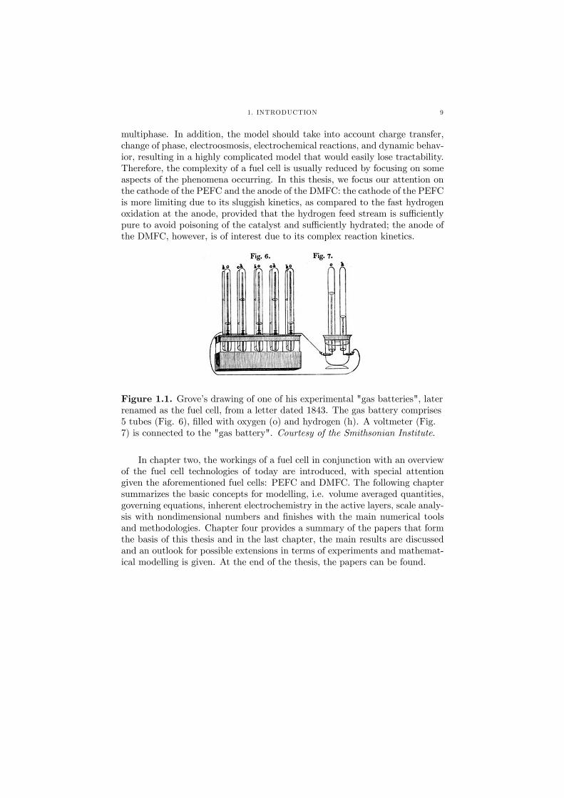
At present, however, despite vast amounts of capital dedicated to R&D,only a few commercial applications can be found, as the production cost re-mains too high to contend with traditional power sources, such as batteries andcombustion engines, without significant market drivers. In addition to reducingthe cost by developing new materials and improved construction techniques, thefuel issue has to be solved satisfactorily: either by fuel storage of pure hydro-gen or by reforming of hydrocarbon fuels. Reductions in cost and advancementof the fuel cell technology are still feasible, though hindered by the highly in-terdisciplinary nature of fuel cells systems, which is one of the reasons whycommercialisation of the fuel cell, despite its effect being discovered as early as1838 by Christian Friedrich Schönbein1 [1], is still in its cradle. Thus, althoughthe first operating fuel cell was constructed by Sir William Robert Grove in1839, a drawing of which is shown in Figure 1.1, it would take more than acentury, until the 1990s, for fuel cell activities to mushroom around the world.
This thesis addresses two types of fuel cells, namely the polymer electrolytefuel cell2 (PEFC) and its sibling, the direct methanol fuel cell (DMFC), withthe aim to further the development of mathematical models for these. Suchmodels are necessary for understanding the inherent transport processes thatoccur in a fuel cell, for improving the design and materials, as well as allow-ing for fast studies of fuel cell systems. The difficulty in modelling a fuel cellstems from the variety of engineering disciplines, ranging from material sci-ence over electrochemistry to fluid dynamics that have to be considered. Amodel, incorporating all of the relevant physics of the various components ina fuel cell, would be three-dimensional, non-isothermal, multicomponent and
1Contrary to common belief, it was C. F. Schönbein who discovered the fuel cell effectand not W. R. Grove [1].
2Also commonly referred to as proton exchange membrane fuel cell (PEMFC) or solidpolymer fuel cell (SPFC).
8
1. INTRODUCTION 9
multiphase. In addition, the model should take into account charge transfer,change of phase, electroosmosis, electrochemical reactions, and dynamic behav-ior, resulting in a highly complicated model that would easily lose tractability.Therefore, the complexity of a fuel cell is usually reduced by focusing on someaspects of the phenomena occurring. In this thesis, we focus our attention onthe cathode of the PEFC and the anode of the DMFC: the cathode of the PEFCis more limiting due to its sluggish kinetics, as compared to the fast hydrogenoxidation at the anode, provided that the hydrogen feed stream is sufficientlypure to avoid poisoning of the catalyst and sufficiently hydrated; the anode ofthe DMFC, however, is of interest due to its complex reaction kinetics.
Figure 1.1. Grove’s drawing of one of his experimental "gas batteries", laterrenamed as the fuel cell, from a letter dated 1843. The gas battery comprises5 tubes (Fig. 6), filled with oxygen (o) and hydrogen (h). A voltmeter (Fig.7) is connected to the "gas battery". Courtesy of the Smithsonian Institute.
In chapter two, the workings of a fuel cell in conjunction with an overviewof the fuel cell technologies of today are introduced, with special attentiongiven the aforementioned fuel cells: PEFC and DMFC. The following chaptersummarizes the basic concepts for modelling, i.e. volume averaged quantities,governing equations, inherent electrochemistry in the active layers, scale analy-sis with nondimensional numbers and finishes with the main numerical toolsand methodologies. Chapter four provides a summary of the papers that formthe basis of this thesis and in the last chapter, the main results are discussedand an outlook for possible extensions in terms of experiments and mathemat-ical modelling is given. At the end of the thesis, the papers can be found.

CHAPTER 2
Fuel cells
In this chapter, the basic principles of a fuel cell are introduced, comprisingthe inner workings as well as an overview of available fuel cell technologies. Aswas mentioned in the introduction, we will focus on the polymer electrolyteand direct methanol fuel cell, of which more details will be given, especially interms of already existing mathematical models.
1. Basic principles
A fuel cell is an electrochemical device that directly converts chemicalenergy into electric energy, and thus is not limited by the Carnot efficiency.
Ano
de
Cat
hode
Fuel
O2,H2O,N2
+- e-
Flow channels Porous backing
Active layer Electrolyte
Oxidant
Figure 2.1. A schematic of a fuel cell.
Fuel cells differ from primary and secondary batteries in how the fuel andoxidant are stored: a primary battery is useless once the stored fuel/oxidant isdepleted; a secondary battery can be recharged, allowing for several recharges;in the fuel cell, the fuel and oxidant are fed continuously and as such does notrequire any recharging. A schematic of a fuel cell is depicted in Figure 2.1.
10

1. BASIC PRINCIPLES 11
The basic cell consists of two porous electrodes3, termed the anode andthe cathode, separated by an electrolyte. These three components constitutethe heart of the fuel cell, also referred to as membrane electrode assembly4
(MEA), sandwiched between two porous backings5 and flow distributors. Theflow distributors usually comprise flow channels machined into a bipolar plate,as illustrated in Figure 2.1, or net-type flow fields. In the course of opera-tion, an oxidant is fed at the inlet on the cathode side and transported to theelectrolyte/cathode interface; the fuel on the other hand, is fed at the anodeinlet and is transported to the electrolyte/anode interface. The reactions atthe electrodes are kept separated by the electrolyte, with electrons that candrive a load through an external circuit, flowing from the anode to the cathodeand ions passing through the electrolyte to close the electric circuit.
The performance of a fuel cell is usually given by a polarization curve,where the cell voltage is related to the current density, or by a power densitycurve, where the power density is given as a function of the current density ofthe cell, as illustrated in Figure 2.2.
I IIIII
Vol
tage
Pow
er d
ensi
ty
Current density
Reversible cell potential
Open circuit potential
Figure 2.2. A schematic of a polarization curve and power density curve.
The polarization curve approaches the open circuit potential as the currentdecreases and not the reversible cell potential as might be expected, when nocurrent is drawn from the cell. This loss in voltage can be attributed to fuelcrossover and internal currents. In Figure 2.2, three regions can be discerned:region I, where the rapid non-linear drop in voltage originates from activationlosses; region II, where the voltage loss is more linear, stemming from ohmiclosses, such as bulk and interface resistances; region III, where the voltage falls
3Also known as active layers.4The MEA is not clearly defined and can sometimes include the porous backings.5These porous layers are sometimes referred to as "gas diffusion layers", which is mis-
leading, since the transport of mass and species is by no means limited to just diffusion andthe gas phase.
12 2. FUEL CELLS
swiftly due to mass transport limitations in the cell. The optimal operatingregime for a fuel cell is up to the maximum of the power density to avoid thesharp decrease in power density that occurs in region III.
2. Overview of fuel cell technologies
The existing fuel cell types can be classified according to the type of elec-trolyte, operating temperature or fuel/oxidant used. According to [2], thereare five types of fuel cells that are viable today; we will add a sixth, namelythe direct methanol fuel cell, to this list:
(1) Polymer electrolyte fuel cell (PEFC): The PEFC operates at low tem-peratures, ∼ 20 − 90oC, and is equipped with a solid polymer elec-trolyte. Vehicles, low power CHP6 systems and mobile applicationare feasible.
(2) Direct methanol fuel cell (DMFC): The DMFC operates at low tem-peratures, ∼ 20− 110oC, and is similar to the PEFC equipped with asolid polymer electrolyte. Potential and present applications includeportable devices.
(3) Alkaline Fuel Cell (AFC): The AFC operates at low temperatures,∼ 60− 220oC, with a liquid electrolyte, comprising OH−. This typeof fuel cell was used on the Apollo craft.
(4) Phosphoric acid fuel cell (PAFC): The PAFC operates at mediumtemperatures, ∼ 150 − 220oC, with a liquid electrolyte, comprisingconcentrated phosphoric acid. This type of fuel cell was the first tobe commercialized. It is well suited for medium scale CHP systems,such as office buildings and schools.
(5) Molten carbonate fuel cell (MCFC): The MCFC operates at high tem-peratures, ∼ 650oC, with an electrolyte, comprising molten carbon-ate. Present and potential applications are for medium to large scaleCHP systems.
(6) Solid oxide fuel cell (SOFC): The SOFC operates at high temper-atures, ∼ 500 − 1000oC, with an electrolyte, comprising a ceramicoxygen conductor. Suitable for all CHP systems.
A more detailed description of these fuel cells can be found in e.g. [2].
6Combined heat and power.

3. POLYMER ELECTROLYTE AND DIRECT METHANOL FUEL CELLS 13
3. Polymer electrolyte and direct methanol fuel cells
Out of the six aforementioned fuel cells, we will focus on the two closelyrelated fuel cells PEFC and DMFC. The main difference between the two is thefuel on the anode side: hydrogen for the former and methanol for the latter. Aschematic of a cross-section in the normal and spanwise direction for these isshown in Figure 2.3 (the streamwise direction is given by the arrows in Figure2.1).
+
-
e- Membrane Active layers
Agglomeratenucleus
Porousbacking
Porousbacking
Flowfield
Anode
Cathode
Polymer electrolyte,e.g. Nafion andliquid water
Carbon particlewith catalyst
Agglomerate
Polytetrafluorethylene(PTFE)
Carbon cloth
Coolingchannels
Figure 2.3. A schematic of a cross-section in a fuel cell. Close-ups of theporous backing and active layers are also shown. The active layer is hereassumed to contain agglomerates [3].
The main components of the cell are:Bipolar plate: The electrochemical reactions that occur at the active layersdepend on a sufficiently fast transport of reactants to, and products from, theactive sites so as to minimize mass transport limitations. Towards this end, thebipolar plates contain grooved channels, which can take a number of differentshapes. Amongst the most common designs today are:
• parallel channels, with only one pass over the porous backing, run incoflow.
• parallel channels, with only one pass over the porous backing, run incounterflow.
• interdigitated channels, where channels are terminated, in order toforce the flow into the porous backing.
• a porous material, such as a net;

14 2. FUEL CELLS
• serpentine flow channels, comprising one long channel with manypasses over the porous backing.
• a combination of some of the above.For the flow fields with channels, the regions between the channels comprise
lands7, where no fluid flow can occur. The porous flow field, in contrast, coversthe whole porous backing due to its porous nature, and thus does not give riseto any ‘dead’ zones for fluid flow. In addition, coolant channels are usuallyincorporated in the bipolar plate or added as an extra layer.Porous backing: The porous backing is made of a composite material, contain-ing carbon cloth/paper and often a hydrophobic agent, such as polytetrafluo-rethylene. It has to meet many requirements:
• electronic conductivity : The material has to be sufficiently conductiveso that the voltage loss is kept at a minimum as well as to facilitatean even current density distribution in the active layers.
• heat conductivity : The heat generated at the active layers has to beremoved through the porous backing to the bipolar plate.
• fluid flow permeability : Fluid flow and the mass transfer of reactantsto and products from the active layer are crucial for the fuel cellperformance.
• wettability : The wettability of the porous backing has to be engineeredin such a way that the membrane is kept sufficiently hydrated, whilstsimultaneously ensuring that flooding of the porous backing does notoccur.
• mechanical stability : The porous backing has to be sufficiently strongto provide support to the MEA as well as keeping the difference inclamping pressure between the land regions and channels at a min-imum. If this stability is not ensured, the porous backing might bepushed up into the flow channels and be unduly compressed under-neath the lands.
Active layer: The active layers are a porous structure, where contact betweenthe catalyst, usually carbon supported platinum, the electrolyte, the carbonand the reactants has to be provided for, in order to facilitate the electrochem-ical reactions. For the PEFC, these are
2H2(g)→ 4H+ + 4e− at the anode, (1)
O2(g) + 4H+ + 4e− → 2H2O at the cathode, (2)
which are termed the hydrogen oxidation reaction (HOR) and the oxygen re-duction reaction (ORR), respectively, and for the DMFC:
CH3OH +H2O → CO2 + 6H+ + 6e− at the anode, (3)
3
2O2 + 6H
+ + 6e− → 3H2O at the cathode. (4)
7Also referred to as ribs.

3. POLYMER ELECTROLYTE AND DIRECT METHANOL FUEL CELLS 15
The methanol is usually fed as a liquid, whereas the hydrogen is fed as agas. Note that these reactions are overall reactions, and that in reality, severalintermediate reaction steps take place.Membrane: The membrane, sandwiched between the active layers, comprisesa solid polymer, usually Nafion R°, which is a perfluorsulphonic acid polymer.The proton conductivity of the membrane hinges on the humidity level, with adecreasing conductivity for lower humidity levels. It is therefore essential thatthe membrane is hydrated throughout operation of the fuel cell.
3.1. Literature overview of models for the PEFC. There is an abun-dance of models available, dealing with both modelling and experiments of thePEFC. Perhaps the first models to provide a simplified treatment of the PEFCwere developed by Bernardi and Verbrugge [4,5] and Springer, Zawodzinski andGottesfeld [6]; a recent contribution is due to Gurau, Barbir and Lui [7]. Thesemodels are one-dimensional, and whilst they are able to address some aspects ofthe three main issues related to fuel cell performance, namely thermal-, watermanagement and mass transfer, they are not able to address these questionsat a local level: that is to say, where oxygen depletion occurs, where there isflooding or inadequate heat removal. Subsequent pseudo-two-dimensional mod-els have tackled some of these issues [8—11], with varying assumptions about thenature of the flow; in these so-called ‘along-the-channel’ models, the resultingequations are ordinary differential equations with the coordinate along the fuelcell as the independent variable. Most recently, techniques of computationalfluid dynamics have been used. Amongst models assuming single-phase gaseousflow, there are 2D isothermal models for the cathode [12—14], 2D isothermalmodels for the whole cell [15—18], and lately three-dimensional models havealso begun to appear [14,19—22,31]. Dutta, Shimpalee and van Zee consideredfirst a straight channel flow under isothermal conditions [19], followed later bya model for flow in a serpentine channel [20]; most recent work extends [19] totake into account heat transfer for a straight channel flow [21]. Costamagnaconsiders non-isothermal conditions and treats the flow distributor as a porousmaterial [22].
Only a few models, however, exist where also the possibility for liquid wa-ter is accounted for [23—32]. He, Yi and Nguyen [23], Natarajan and Nguyen[24], Wang, Wakayama and Okada [25], You and Liu [26], Wang, Wang andChen [27] focus on the mass transport limitations and water management ina two-dimensional cathode and assume isothermal conditions. All three is-sues mentioned above, are considered for the whole cell by Djilali and Lu [28],Janssen [29] and Wöhr et al. [30] for a one-dimensional geometry and by Bern-ing and Djilali [31] and Mazumder and Cole [32] for a three-dimensional geom-etry.
Most of the models are validated on a global scale with polarization curves,which are unable to capture the current density distributions on a local level;only Lum [14] validated her models with both global polarization curves andlocal current density distributions obtained from a segmented cell.
16 2. FUEL CELLS
3.2. Literature overview of models for the DMFC. There are al-ready some models, mostly one-phase, of the DMFC that aim to describe theprocesses occurring, including the electrochemistry [33—51]. Most of these con-sider mass transfer in both the gas-backing layer and the active layer [33, 37—41,44—49,51], but only a few consider streamwise effects [33,37,40,51].
The carbon dioxide gas is usually neglected in DMFC modelling literature,even though the evolution of gas at the anode can be observed in most practicalDMFC applications. Most recently, however, two models considering coexistinggas and liquid phases have been published [50,51]. Wang and Wang [50] applya multiphase mixture theory for porous media [52] to the porous backings,active layers of both the anode and cathode as well as the membrane of a two-dimensional DMFC, and treat the flow channels on the anode side with a flux-drift model to account for the gas slug flow. They use a simplified expressionfor the anode kinetics: a Tafel slope with a reaction order that is zero or onedepending on the methanol concentration exceeding a threshold value. Themodel by Divisek et al. [51] is also two-dimensional, but for a cross-sectionat a given streamwise position and is limited to the porous backings, activelayers and membrane of the cell. Common for both these published two-phasemodels is that they are only validated with global polarization curves, thuslacking any experimental details about the two-phase flow, such as e.g. theamount of gas in the flow channels. Such polarization curves are ill suited forvalidating the increasing amount of constitutive relations that arise to close thegoverning equations when proceeding from a one-phase treatment to a modelthat handles two-phase flow.
CHAPTER 3
Basic concepts
Thus far, the basic principles of fuel cells have been introduced and we haveseen that a fuel cell comprises several parts: flow distributors, porous backings,active layers on the anode and cathode side and a membrane. In addition,the available fuel cell technologies of today have been presented, with a morethorough discussion of the PEFC and DMFC. In this chapter, we proceed withthe mathematical tools for modelling of the these two fuel cells. The aforemen-tioned parts of the fuel cell have to be modelled and coupled to each other in aconvenient way. The porous backings as well as the net-type flow distributorscan be treated as porous media, for which volume averaged quantities are em-ployed. We start with the most fundamental definitions of these and continuewith the main governing equations for all parts of the fuel cell, both one- andtwo-phase, that we have used. The treatment of the inherent electrochemistryin the active layers is then summarized.
1. Volume averaging
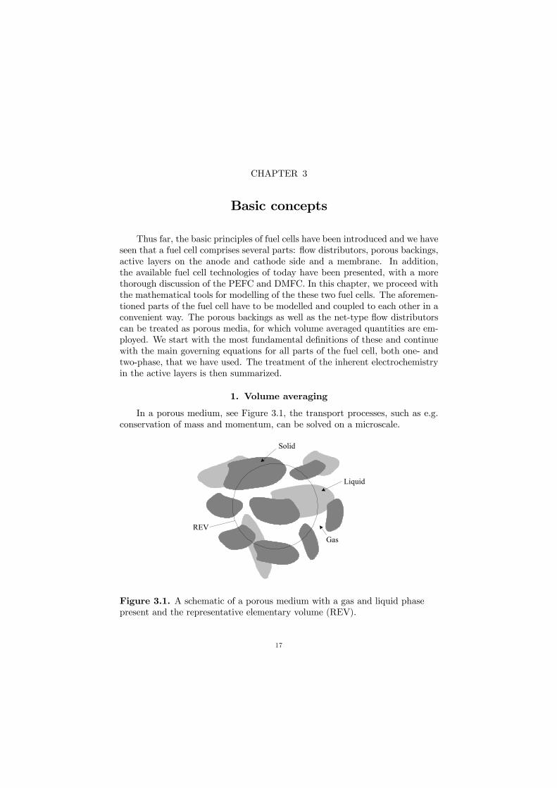
In a porous medium, see Figure 3.1, the transport processes, such as e.g.conservation of mass and momentum, can be solved on a microscale.
Liquid
Gas
Solid
REV
Figure 3.1. A schematic of a porous medium with a gas and liquid phasepresent and the representative elementary volume (REV).
17
18 3. BASIC CONCEPTS
This, however, requires that we solve for every pore throughout the porousmedium, which is computationally expensive as well as time consuming, not tomention that the often complex structure has to be known a priori. A moreconvenient approach is to average the microscale equations over a representativeelementary volume (REV), resulting in macroscale equations. For simplicity,we will here assume that we deal with a two-phase system8, comprising a liquid(l), a gas (g), and a stationary and rigid solid phase.
For the macroscale description, we define the superficial average of a quan-tity φ(k) as D
φ(k)E=1
V
ZVφ(k)dV, (5)
where V is the total volume of the REV and φ(k) is the value of the quantity φ(scalar, vector, tensor) in phase k (k = l, g). The intrinsic average is defined asD
φ(k)E(k)
=1
V(k)ZV(k)
φ(k)dV, (6)
where V(k) is the volume of phase k in the REV. Introducing the porosity
γ =V(g) + V(l)
V , (7)
and the saturation of phase k
s(k) =V(k)
V(g) + V(l) , (8)
the two averages are related throughDφ(k)
E= s(k)γ
Dφ(k)
E(k). (9)
Here, we have also used that φ(k) is zero in all the other phases than k. Wewill retain this notation for the one-phase description of porous flow but omith.i for the corresponding two-phase formulations to save on notation.
2. Governing equations
The main governing equations for the flow distributors and porous backingare summarized below for one- and two-phase flow for the cathode of the PEFCand the anode of the DMFC. For the one-phase flow treatment, we differentiatebetween plain and porous flow, where the plain flow occurs in the flow channelsof the flow field and the porous flow in the porous backing as well as in theflow field, if a net-type flow distributor is used. For the two-phase flow, we willlist the governing equations for a separate flow (PEFC, Paper 3 and 4) and amultiphase mixture (DMFC, Paper 7) approach. For brevity, we refer to thepapers for the constitutive relations and boundary conditions, which togetherwith the governing equations constitute closed systems.
8The term "two-phase", referring to the mobile liquid and gas phase, is somewhat mis-leading, since we actually consider three phases.

2. GOVERNING EQUATIONS 19
For the PEFC, the flow will remain gas-phase as long as the water va-por pressure does not exceed the saturation pressure, whereas for a liquid-fedDMFC, the flow will be in liquid form until the carbon dioxide stemming fromthe oxidation at the active layer evolves as gas. A model based on one-phaseflow will thus not be able to account for the liquid water (PEFC) or the gas(DMFC), but can nonetheless give valuable information (Paper 1, 2 and 5).
2.1. Plain Flow. The flow distributor can take many shapes, dependingon the requirements of the fuel cell: flow channels machined into a bipolarplate, comprising e.g. interdigitated, parallel or serpentine channels. In theflow channels, we solve for continuity of mass and momentum, given by
∇ · (ρv) = 0, (10)
∇ · (ρv ⊗ v) = −∇µp+
2
3µ∇ · v
¶+∇ ·
³µ³(∇v) + (∇v)T
´´, (11)
where v is the velocity, ρ is the density, p is the pressure and µ is the dynamicviscosity. The transport equations for the ternary gas mixture, comprisingoxygen, water and nitrogen are
∇ ·µρv
µwO2
wH2O
¶¶= ∇ ·
µρD
·∇wO2
∇wH2O
¸¶, (12)
where wO2 and wH2O are the mass fractions of oxygen and water and D isthe diffusion tensor. To obtain the corresponding formulation for the DMFC,substitute MeOH = O2, CO2 = H2O.
2.2. Porous flow. Conservation of mass and momentum in the porousbacking or in a net-type flow field is given respectively by
∇ ·³hρi(g) hvi
´= 0, (13)
∇ ·³hρi(g) hvi⊗ hvi
´+ µK−1 · hvi = −∇
µhpi(g) + 2
3
µ
γ∇ · hvi
¶+∇ ·
µµ
γ
³∇ hvi+ (∇ hvi)T
´¶, (14)
whereK is the permeability tensor. An alternative formulation for conservationof momentum is Darcy’s law with the Forchheimer and Brinkman extension
hvi = −κµ∇ hpi(g) + κ∇2
µhviγ
¶− F hvi , (15)
where F is the Forchheimer correction tensor.The species transport equations are described by
∇ ·Ãhρi(g) hvi
ÃhwO2i
(g)
hwH2Oi(g)
!!= ∇ ·
Ãhρi(g) γ hDi(g)
"∇ hwO2i
(g)
∇ hwH2Oi(g)
#!,
(16)
20 3. BASIC CONCEPTS
where hDi(g) is the total mass diffusion tensor, containing contributions froman intrinsic effective mass diffusion tensor and an intrinsic hydrodynamic dis-persion tensor. For a more detailed discussion of these, see paper 1. To ob-tain the corresponding formulation for the DMFC, substitute MeOH = O2,CO2 = H2O and (l) = (g).
2.3. Conservation of charge. Conservation of charge together with Ohm´slaw gives
∇2φ = 0, (17)
where φ is the electric potential of the solid phase in the porous backings orthe ionic phase in the membrane. This equation constitutes a simplification ofthe proton transport in the membrane.
2.4. Separate flow model. The PEFC is usually operated at high rela-tive humidities or even at two-phase conditions since the membrane conductiv-ity hinges on the membrane being sufficiently hydrated. To account for a liquidphase in addition to the gas phase, we apply a separate flow model (Paper 3and 4), where we treat the liquid and gas phase as immiscible.
The solubility of nitrogen and oxygen is sufficiently small to allow the liquidphase to be treated as pure liquid water. In the porous backing of the cathode,we solve for the conservation of mass and momentum of the liquid and gasphase:
∇ ·³ρ(g)v(g)
´= − ·
mH2O, (18)
∇ ·³ρ(l)v(l)
´=
·mH2O, (19)
∇p(g) = − µ(g)
κκ(g)rel
v(g), (20)
∇p(l) = − µ(l)
κκ(l)rel
v(l), (21)
where ρ(g,l) denote the phase densities, v(g,l) = (u(g,l), v(g,l)) are the phase ve-locities,
·mH2O is the interface mass transfer of water between the gas and liquid
phase, p(g,l) are the phase pressures, µ(g,l) are the phase dynamic viscosities, κis the permeability and κ
(g,l)rel are the relative permeabilities of the phases.
In addition, we solve for a ternary mixture of water, nitrogen and oxygenin the gas phase
∇ ·"n(g)O2
n(g)H2O
#+
·0
·mH2O
¸= 0, (22)
with the componential mass fluxes"n(g)O2
n(g)H2O
#= ρ(g)v(g)
"w(g)O2
w(g)H2O
#− ρ(g)γ
32 (1− s)D(g)
"∇w(g)O2
∇w(g)H2O
#, (23)
2. GOVERNING EQUATIONS 21
where D(g) is a multicomponent mass diffusion tensor, γ is the porosity, s isthe liquid saturation and w
(g)H2O
and w(g)O2
are the mass fraction of water andoxygen in the gas phase, respectively. The heat transfer is given by
−∇ · (kc∇T ) = Hvap·mH2O + σc (∇φs)
2 ; (24)
here T is the temperature (assuming thermal equilibrium), kc is a thermalconductivity and Hvap is the enthalpy of vaporization. The terms on the RHSof Eq. 24 account for the heat of vaporization and ohmic heating. Note thatthe convective heat transfer has been omitted in Eq. 24, since this term wasfound to be negligible compared to the heat conduction (Paper 3 and 4).
The governing equations are simplified by removing the liquid pressure viathe definition of the capillary pressure p(c) ≡ p(g)−p(l), in the two-phase region.By taking the gradient of the capillary pressure, and combining Eqs. 20 and21, the liquid velocity is obtained:
v(l) = mv(g) −D(c)∇s, (25)
where m is the mobility of the liquid phase andD(c) can be viewed as a capillarydiffusion coefficient
m =κ(l)relµ
(g)
κ(g)relµ
(l), (26)
D(c) = −κκ(l)rel
µ(l)dp(c)
ds. (27)
It is assumed that the capillary pressure is only a function of saturation; p(c) =p(c)(s).
2.5. Multiphase mixture model. For a liquid-fed anode, the flow throughthe anode will remain liquid as long as no current is drawn from the cell. Assoon as a current is drawn, carbon dioxide is produced from the oxidationreaction at the active layer of the anode. Provided that the carbon dioxidepartial pressure is sufficiently high and nucleation can occur, gas will evolve.Usually, the liquid dilute methanol/water mixture fuel is recirculated, whencethe entering liquid fuel is saturated with carbon dioxide. Incorporating theseeffects calls for a two-phase model, where conservation of mass, momentum andspecies are treated (Paper 7). For this purpose, we apply a multiphase mixtureformulation for porous flow, derived by [52]. The ternary gas and liquid phasesare assumed to be in equilibrium, comprising carbon dioxide, methanol andwater.
We solve for the continuity of mass and momentum of the liquid and gasphase
∇ · (ρv) = 0, (28)
∇p = −µκv+ ρkg, (29)
22 3. BASIC CONCEPTS
where ρ,v, p, µ and ρk are the mixture density, the mixture velocity, themixture pressure, mixture dynamic viscosity and kinematic mixture density,respectively, κ is the absolute permeability and g is the gravity. When refer-ring to the properties of the individual liquid and gas phases, we will use thesuperscripts (l) and (g), respectively. The mixture variables are defined as
ρ = ρ(l)s+ ρ(g)(1− s), (30)
ρk = λ(l)ρ(l) + λ(g)ρ(g), (31)
ρv = ρ(l)v(l) + ρ(g)v(g), (32)
µ =ρ(l)s+ ρ(g)(1− s)
ρ(l)κ(l)rel/µ
(l) + ρ(g)κ(g)rel /µ
(g), (33)
λ(l) =ρ(l)κ
(l)rel/µ
(l)
ρ(l)κ(l)rel/µ
(l) + ρ(g)κ(g)rel /µ
(g), (34)
λ(g) = 1− λ(l). (35)
The superficial phase velocities of the liquid and gaseous phase can be foundfrom the relations
ρ(l)v(l) =λ(l)λ(g)κρ
µ
³∇p(c) +
³ρ(l) − ρ(g)
´g´+ λ(l)ρv, (36)
ρ(g)v(g) = −λ(l)λ(g)κρ
µ
³∇p(c) +
³ρ(l) − ρ(g)
´g´+ λ(g)ρv. (37)
Species transfer is accounted for by
∇ ··NMeOH
NCO2
¸= 0, (38)
with·NMeOH
NCO2
¸= ρv
Ãλ(l)
M (l)
"x(l)MeOH
x(l)CO2
#+
λ(g)
M (g)
"x(g)MeOH
x(g)CO2
#!−Ã
sρ(l)γ hMi(l)¡M (l)
¢2"∇x(l)MeOH∇x(l)CO2
#+(1− s)ρ(g)γ hMi(g)¡
M (g)¢2
"∇x(g)MeOH∇x(g)CO2
#!+Ã
1
M (l)
"x(l)MeOH
x(l)CO2
#− 1
M (g)
"x(g)MeOH
x(g)CO2
#!λ(l)λ(g)κρ
µ
³∇p(c) +
³ρ(l) − ρ(g)
´g´;
(39)
here, NMeOH and NCO2 are the total molar fluxes of methanol and carbondioxide, hMi(l,g) , λ(l) and λ(g) are the diffusion tensors and mobilities of theliquid and gas phase, respectively, p(c) is the capillary pressure, p(g) is thepressure in the gas phase, ρ(k)and x
(k)i are the density and molar fractions of
species i of phase k, respectively.

3. ELECTROKINETICS AND THE ACTIVE LAYERS 23
The capillary pressure is defined as
p(c) = p(g) − p(l), (40)
and the mixture pressure
∇p = ∇p(l) + λ(g)∇p(c). (41)
3. Electrokinetics and the active layers
The active layers are not resolved, but rather treated as boundary or in-terface conditions. For the DMFC (Paper 5 and 7), however, the changes inpotential and concentration inside the active layer of the anode are still ac-counted for and can, if so desired, be computed a posteriori.
3.1. Polymer electrolyte fuel cell. In paper 1, a Tafel law given by [54]was applied for the current density at the cathode
i =aρ
Mexp
µαcFηcRT
¶, (42)
where αc is the transfer coefficient of the oxygen reduction reaction, ηc is theoverpotential for the oxygen reaction (defined positive) and a is a constantrelated to the exchange current density and oxygen reference concentration forthe ORR.
In paper 2, the volumetric current density iv for the cathode, given by [3],was approximated as
iv = Ai0,c¡1− γpol
¢(1− γactive) exp
µ−αrFRT
ηc
¶Fc(g)O2
crefO2
(43)
whereAi0,c is the volumetric exchange current density in the agglomerates, γpolis the volume fraction of the polymer electrolyte in the agglomerate nucleus,c(g)O2= w
(g)O2
ρ(g)/MO2 is the molar concentration of oxygen, αr is the cathodictransfer coefficient for the ORR, n is the number of electrons consumed inthe ORR per oxygen molecule, ηc is the overpotential at the cathode (definednegative), and γactive is the volume fraction of pores in the active layer. F isthe nucleus effectiveness factor, defined as
F =3
Υr
µ1
tanh(Υr)− 1
Υr
¶, (44)
with Υ given by
Υ =
sAi0
¡1− γp
¢exp
¡−αrF
RT η¢
nFD, (45)
where D is an effective oxygen permeability in the agglomerates and r is theradius of the agglomerate nucleus. This agglomerate model was validated by[53] for a small PEFC with an area of 2 cm2. The total current density is thenlocally given by ic = ivhactive. Jaouen et al. [3] discerned four different regimes,where the Tafel slope doubles or even quadruples, and subsequently suppliedthe experimental validation to support these [53]. In regime 1, the active layer

24 3. BASIC CONCEPTS
is controlled by Tafel kinetics and is first order in the oxygen concentration.Regime 2 displays a doubling of the Tafel slope, due to the active layer beinggoverned by Tafel kinetics and oxygen diffusion in the agglomerates, but stillremains first order in the oxygen concentration. A doubling of the Tafel slopeis observed in the third regime, where the active layer is controlled by theTafel kinetics, in addition to proton migration. The oxygen dependence hereis half-order. The final regime, the fourth, shows a quadrupling of the Tafelslope, and is attributable to an active layer controlled by Tafel kinetics, protonmigration and oxygen diffusion in the agglomerates. The oxygen dependenceis half-order, as in regime 3.
In paper 3, we tried to adapt the agglomerate model to a polarizationcurve obtained from a segmented cell, equipped with a net-type flow field, butit turned out that the agglomerate model reduced to
ic = ζ1(1− s)x(g)O2exp(−ζ2ηc), (46)
where ζ1 and ζ2 are the two parameters adapted. Essentially this mean thatthe nucleus effectiveness factor F = 1, which we surmise is due to the thinMEA (Gore Primea 5510) that was used in the segmented cell. In paper 4, theparameter adapted current density was also applied.
3.2. Direct methanol fuel cell. In paper 5, an expression for the currentdensity was found from parameter-adaption to experimental data [55]
hii = A³hcMeOHi(l)
´B exp¡αAFRT (EA −E0)
¢1 + exp
¡αAFRT (EA −E0)
¢ . (47)
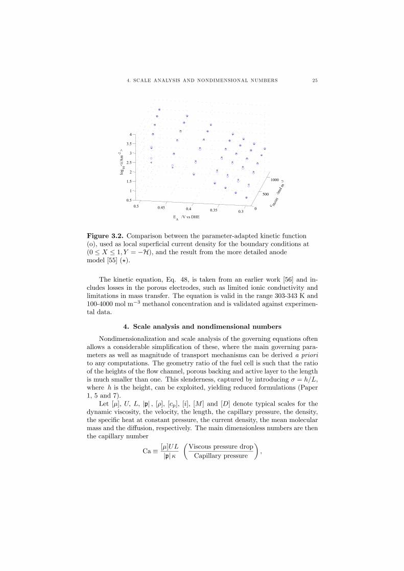
Figure 3.2 shows that this expression for the local current density correlateswell to the data from the electrode model [55] for 0.3V≤ E ≤ 0.51 V and 50mol m−3 ≤ hcMeOHi(l) ≤ 1000 mol m−3.
In paper 7, the current density at the active layer is given [56], as
i(x(l)MeOH, T,M
(l), EA) =exp
¡αAFRT (EA − EA)
¢1 +
exp³αAF
RT (EA−EA)´
ilim
, (48)
EA = c1 − c2T, (49)
ilim = tanh
x(l)MeOH
¯y=−hp
ρ(l)
M (l)¯y=−hp c3
µEAc4
¶ϑ ¡c5T
2 − c6T + c7¢, (50)
ϑ = c8 tanh
x(l)MeOH
¯y=−hp
ρ(l)
M (l)¯y=−hp c9
, (51)
where i is the local current density, EA is the anode potential measured at theactive layer/membrane interface versus a reference electrode (EA = 0.2−0.7 V[56]), αA is a measured Tafel slope , and ci are experimentally fitted parameters.
4. SCALE ANALYSIS AND NONDIMENSIONAL NUMBERS 25
0
500
1000
0.30.350.40.450.50.5
1
1.5
2
2.5
3
3.5
4
c MeO
H /
mol
m-3
EA
/V vs DHE
log 10
<i/A
m-2
>
Figure 3.2. Comparison between the parameter-adapted kinetic function(o), used as local superficial current density for the boundary conditions at(0 ≤ X ≤ 1, Y = −H), and the result from the more detailed anodemodel [55] ( ).
The kinetic equation, Eq. 48, is taken from an earlier work [56] and in-cludes losses in the porous electrodes, such as limited ionic conductivity andlimitations in mass transfer. The equation is valid in the range 303-343 K and100-4000 mol m−3 methanol concentration and is validated against experimen-tal data.
4. Scale analysis and nondimensional numbers
Nondimensionalization and scale analysis of the governing equations oftenallows a considerable simplification of these, where the main governing para-meters as well as magnitude of transport mechanisms can be derived a priorito any computations. The geometry ratio of the fuel cell is such that the ratioof the heights of the flow channel, porous backing and active layer to the lengthis much smaller than one. This slenderness, captured by introducing σ = h/L,where h is the height, can be exploited, yielding reduced formulations (Paper1, 5 and 7).
Let [µ], U, L, |p| , [ρ], [cp], [i], [M ] and [D] denote typical scales for thedynamic viscosity, the velocity, the length, the capillary pressure, the density,the specific heat at constant pressure, the current density, the mean molecularmass and the diffusion, respectively. The main dimensionless numbers are thenthe capillary number
Ca ≡ [µ]UL|p|κ
µViscous pressure dropCapillary pressure
¶,

26 3. BASIC CONCEPTS
the Damköhler numbers (F is Faraday’s constant)
Λ ≡ [i][M ]
[ρ]UF
µReaction rate
Mass transport rate
¶,
Ω ≡ Λ
σ
µReaction rate
Mass transport rate
¶,
the Darcy number
Da ≡ κ
L2(Dimensionless permeability) ,
the reciprocal of the reduced Reynolds number
∆ ≡ 1
Reσ2,
the Froude number
Fr ≡ U2
gL
µInertia forceGravity force
¶,
the gravillary number
Gl ≡ ρ(l)gl
|p|
µGravitational pressureCapillary pressure
¶,
the gravitary number
Gr ≡ [µ]U
[ρ]gκ
µViscous pressure dropGravitational pressure
¶,
the Peclet number for heat transfer
Pe(heat) ≡ U [ρ]L[cp]
k
µHeat convectionHeat conduction
¶,
and mass transfer
Pe(mass) ≡ UL
[D]
µBulk mass transfer
Diffusive mass transfer
¶,
the Reynolds number
Re ≡ [ρ]LU[µ]
µInertia forceViscous force
¶,
the Schmidt number
Sc ≡ [µ]
[ρ][D]
µMomentum diffusivityMass diffusivity
¶.

5. NUMERICAL TOOLS AND METHODOLOGIES 27
5. Numerical tools and methodologies
To solve the mathematical models for the PEFC and DMFC, various meth-ods were adopted, a summary of which is given below.
5.1. Keller Box discretization scheme. Invoking the slenderness ofthe fuel cells, the elliptic governing equations were reduced to parabolic for across-section in the normal and streamwise directions, for which the Keller Boxdiscretization scheme [57] is suitable (Paper 1 and 7). The scheme leads toa block tridiagonal matrix, allowing fast computations. The resulting systemof non-linear equations is solved with a Newton-Raphson-based algorithm inMATLAB 6 (see [58] for details).
5.2. Modified Box discretization method. The Modified Box dis-cretization scheme [59] is a reduced version of the aforementioned Keller Box,and requires more effort to derive (Paper 7). The scheme leads to a block tridi-agonal matrix, allowing fast computations. The resulting system of non-linearequations is solved with a Newton-Raphson-based algorithm in MATLAB 6.
5.3. Femlab 2.3. FEMLAB 2.3 (see [60] for details), is a commercialfinite element solver for a wide variety of engineering applications. It was usedto verify several of the reduced DMFC models (Paper 5 and 7) as well as modela cross-section in the normal and spanwise directions for the PEFC (Paper 3and 4).
5.4. CFX 4.4. A commercial computational fluid dynamics code, CFX-4.4 (see [61] for details), based on finite volumes, was used for three dimensionalcomputations of various flow fields (Paper 2), as well as for verification of areduced model (Paper 5).
5.5. Maple 7. Maple 7 (see [62] for details) was used to secure closedform solutions for the asymptotic analyses, to produce Fortran code and tofind analytical solutions, where applicable.
CHAPTER 4
Summary of results
1. Polymer electrolyte fuel cells
Four models for the cathode have been derived and analyzed. The first (Pa-per 1) sees the derivation of a gas phase isothermal 2-D model for conservationof mass, momentum and species for the cathode followed by nondimension-alization and an asymptotic analysis. The fact that the geometry is slender,see Figure 4.1, allows the use of a narrow-gap approximation, leading to asimplified formulation.
y
x
Inlet
Flow channel
Porous Backing
Active region
Figure 4.1. A schematic of the cathode.
Inspite of the highly non-linear coupling between the velocity variablesand the mole fractions, an asymptotic treatment of the problem indicates thatoxygen consumption and water production can be described rather simply inthe classical lubrication theory limit with the reduced Reynolds number as asmall parameter. In general, however, the reduced Reynolds number is O (1),requiring a numerical treatment; this is done using the Keller-Box discretiza-tion scheme. The analytical and numerical results are compared in the limitmentioned above, and further results are generated for varying inlet velocityand gas composition, channel width and porous backing thickness, pressureand current density. In addition, polarization surfaces, constituting a novel,compact way to present fuel cell performance, which take into account geomet-rical, hydrodynamical and electrochemical features, are introduced. One suchpolarization surface is shown in Figure 4.2 for varying inlet molar fractions ofoxygen and water, from which it is clear, that the greater the oxygen contentin the gas stream at the inlet of the cathode, the greater will be the currentdensity.
28

1. POLYMER ELECTROLYTE FUEL CELLS 29
Figure 4.2. Polarization surfaces for pout = 1 atm with: (a) xinO2= 1,
xinH2O = 0; (b) xinO2= 0.21, xinH2O = 0; (c) x
inO2= 0.13, xinH2O = 0.36.
The second model (Paper 2) is similar to the first, with the important dis-tinction that it is extended to account for a fully three dimensional cathode.The aim of this model was to compare the performance of different flow dis-tributors (parallel coflow, parallel counterflow, interdigitated, foam) for a givencell at a given potential, in terms of four different quantities: the obtained av-erage current density, power density, standard deviation of the current densitydistribution and pressure drop. The results show that the interdigitated flowdistributor can sustain the highest current densities, as depicted in Figure 4.3,but at a higher pressure drop than the counterflow and coflow channels. Fur-thermore, to function properly, the interdigitated channels would have to be incontact with the porous backing in such a way that channeling effects are keptat a minimum; given the high velocities required, even the slightest gap mightlead to most of the flow going through the gap and not through the porousbacking, with a resulting loss of power density. A foam distributor is able togive the lowest standard deviation for the current at high current densities,but care should be taken as to its permeability to avoid an unreasonably highpressure drop.
These two models (Paper 1 and 2) are limited to gas-phase flow and isother-mal conditions. Non-isothermal effects and the liquid water were added via aseparate flow model (Paper 3) for a two-dimensional cross-section, see Figure2.3.

30 4. SUMMARY OF RESULTS
0 0.5 1 1.5 2 2.5 3 3.5 40.2
0.3
0.4
0.5
0.6
0.7
0.8
0.9
1
<i>avg/Acm-2
E cell/V
ξ increasing
Figure 4.3. Polarisation curves for the different flow distributors atstoichiometry ξ = 1.5, 3, 5: coflow channels (o), counterflow channels (∇),interdigitated channels (x), foam (+).
This model is then analyzed and solved numerically under three differentthermal and two hydrodynamic modelling assumptions:
a) an effective heat conductivity with a capillary pressure of O(104)Nm−2 in the porous backings [27];
b) isothermal conditions with a capillary pressure of O(104) Nm−2 inthe porous backings [27];
c) thermal bulk and contact resistances with a capillary pressure ofO(104) Nm−2 in the porous backings [27];
d) an effective heat conductivity with an alternative capillary pressureof O(40) Nm−2 in the porous backings [24];
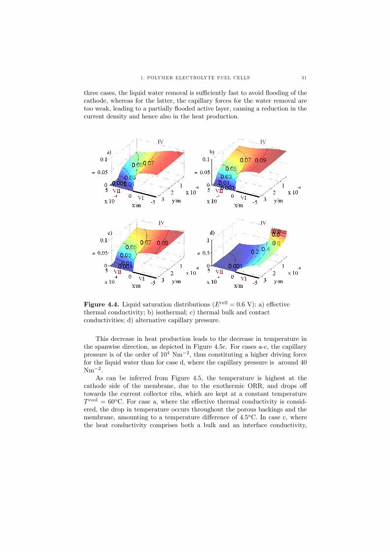
The consequences of these are then discussed in terms of thermal and watermanagement and cell performance. The study is motivated by recent experi-mental results that suggest the presence of previously unreported, and thus un-modeled, thermal contact resistances between the components of a PEFC [63],and the discrepancy in the value for the capillary pressure that is used by dif-ferent authors when modelling the two-phase flow in a PEFC. In the three casesthat deal with varying thermal conditions (a-c), see Figure 4.4, liquid satura-tions of around 10% are obtained at the cathode active layer for 1000 mAcm−2
and a cell voltage of 0.6 V, in contrast to almost 50 % (locally up to 100%)for case d, where the alternative capillary pressure is considered. For the first
1. POLYMER ELECTROLYTE FUEL CELLS 31
three cases, the liquid water removal is sufficiently fast to avoid flooding of thecathode, whereas for the latter, the capillary forces for the water removal aretoo weak, leading to a partially flooded active layer, causing a reduction in thecurrent density and hence also in the heat production.
Figure 4.4. Liquid saturation distributions (Ecell = 0.6 V): a) effectivethermal conductivity; b) isothermal; c) thermal bulk and contactconductivities; d) alternative capillary pressure.
This decrease in heat production leads to the decrease in temperature inthe spanwise direction, as depicted in Figure 4.5c. For cases a-c, the capillarypressure is of the order of 104 Nm−2, thus constituting a higher driving forcefor the liquid water than for case d, where the capillary pressure is around 40Nm−2.
As can be inferred from Figure 4.5, the temperature is highest at thecathode side of the membrane, due to the exothermic ORR, and drops offtowards the current collector ribs, which are kept at a constant temperatureT cool = 60oC. For case a, where the effective thermal conductivity is consid-ered, the drop in temperature occurs throughout the porous backings and themembrane, amounting to a temperature difference of 4.5oC. In case c, wherethe heat conductivity comprises both a bulk and an interface conductivity,
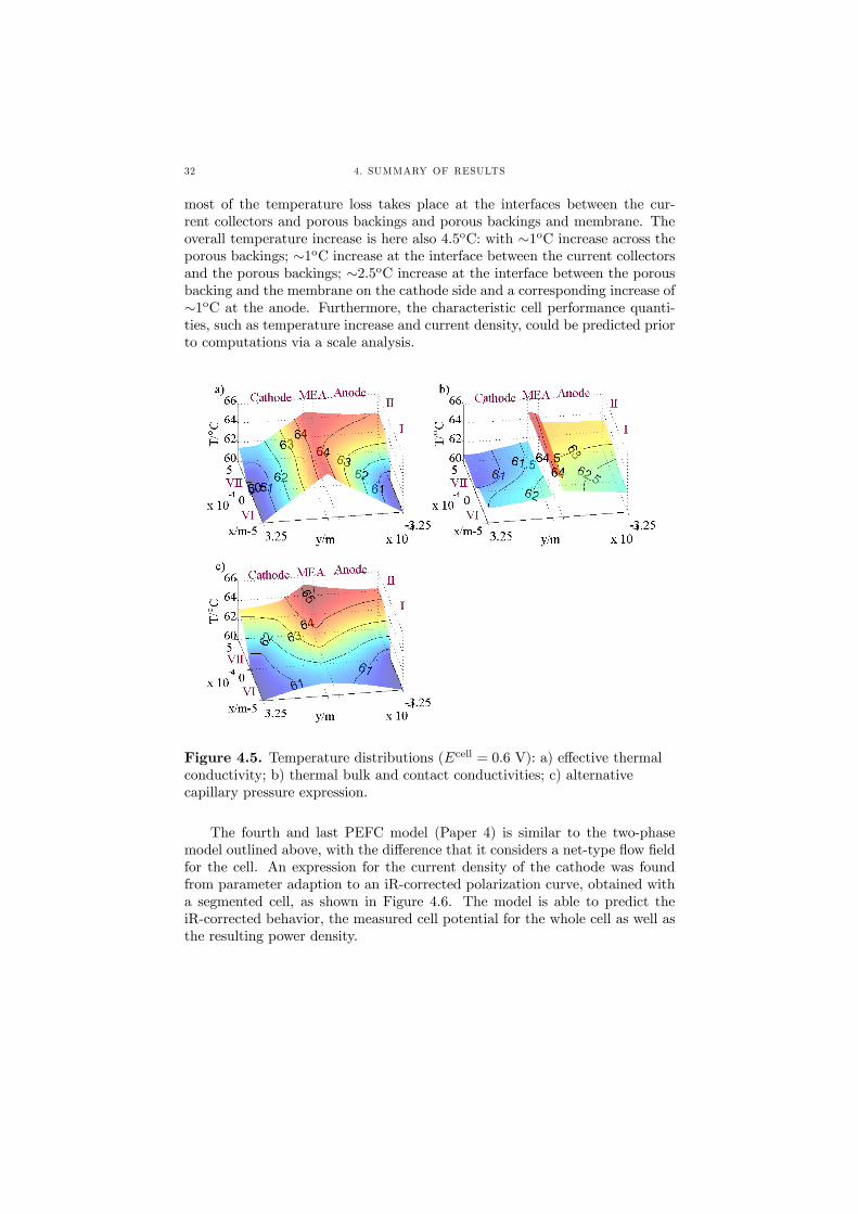
32 4. SUMMARY OF RESULTS
most of the temperature loss takes place at the interfaces between the cur-rent collectors and porous backings and porous backings and membrane. Theoverall temperature increase is here also 4.5oC: with ∼1oC increase across theporous backings; ∼1oC increase at the interface between the current collectorsand the porous backings; ∼2.5oC increase at the interface between the porousbacking and the membrane on the cathode side and a corresponding increase of∼1oC at the anode. Furthermore, the characteristic cell performance quanti-ties, such as temperature increase and current density, could be predicted priorto computations via a scale analysis.
Figure 4.5. Temperature distributions (Ecell = 0.6 V): a) effective thermalconductivity; b) thermal bulk and contact conductivities; c) alternativecapillary pressure expression.
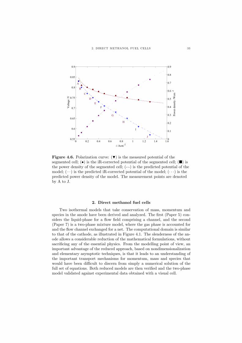
The fourth and last PEFC model (Paper 4) is similar to the two-phasemodel outlined above, with the difference that it considers a net-type flow fieldfor the cell. An expression for the current density of the cathode was foundfrom parameter adaption to an iR-corrected polarization curve, obtained witha segmented cell, as shown in Figure 4.6. The model is able to predict theiR-corrected behavior, the measured cell potential for the whole cell as well asthe resulting power density.
2. DIRECT METHANOL FUEL CELLS 33
0 0.2 0.4 0.6 0.8 1 1.2 1.4 1.60.55
0.6
0.65
0.7
0.75
0.8
0.85
0.9
i /Acm-2
Vol
tage
/V
0
0.1
0.2
0.3
0.4
0.5
0.6
0.7
0.8
0.9
Pow
er d
ensi
ty /W
cm-2
E
B
C
D
F
G
H
I
J
A
Figure 4.6. Polarization curve: (H) is the measured potential of thesegmented cell; (•) is the iR-corrected potential of the segmented cell; (¥) isthe power density of the segmented cell; (-·-) is the predicted potential of themodel; (–) is the predicted iR-corrected potential of the model; (· · ·) is thepredicted power density of the model. The measurement points are denotedby A to J.
2. Direct methanol fuel cells
Two isothermal models that take conservation of mass, momentum andspecies in the anode have been derived and analyzed. The first (Paper 5) con-siders the liquid-phase for a flow field comprising a channel, and the second(Paper 7) is a two-phase mixture model, where the gas phase is accounted forand the flow channel exchanged for a net. The computational domain is similarto that of the cathode, as illustrated in Figure 4.1. The slenderness of the an-ode allows a considerable reduction of the mathematical formulations, withoutsacrificing any of the essential physics. From the modelling point of view, animportant advantage of the reduced approach, based on nondimensionalizationand elementary asymptotic techniques, is that it leads to an understanding ofthe important transport mechanisms for momentum, mass and species thatwould have been difficult to discern from simply a numerical solution of thefull set of equations. Both reduced models are then verified and the two-phasemodel validated against experimental data obtained with a visual cell.
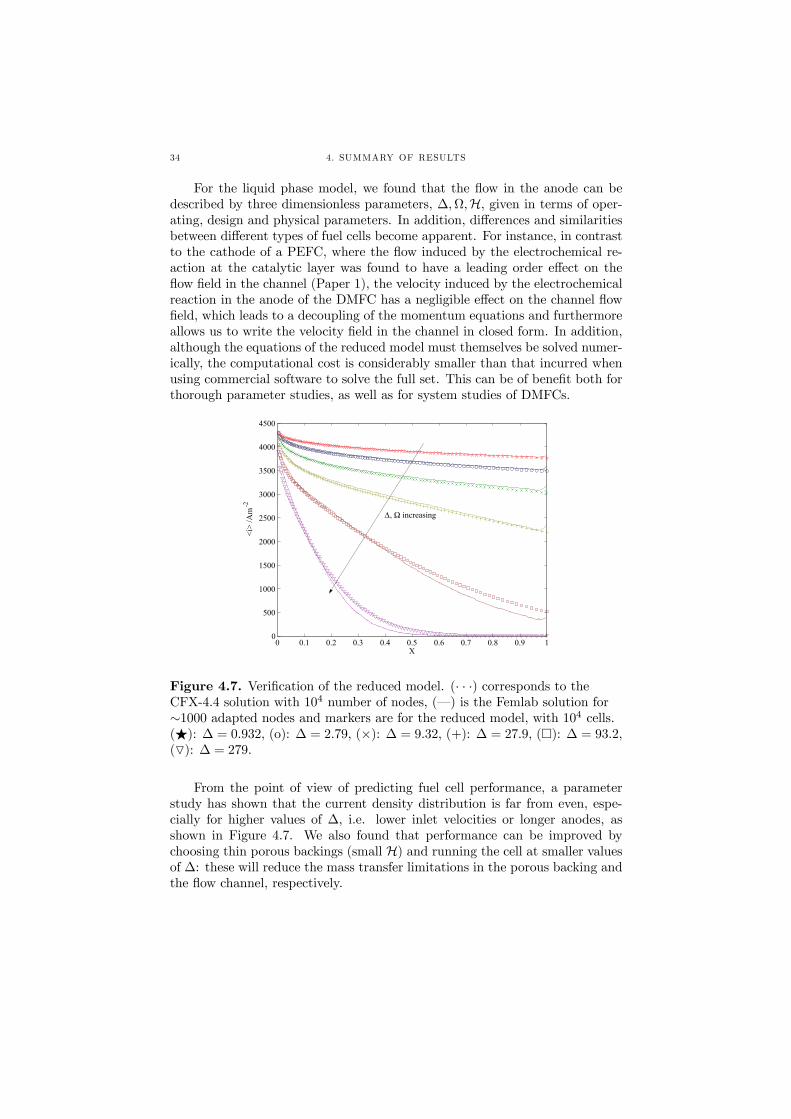
34 4. SUMMARY OF RESULTS
For the liquid phase model, we found that the flow in the anode can bedescribed by three dimensionless parameters, ∆,Ω,H, given in terms of oper-ating, design and physical parameters. In addition, differences and similaritiesbetween different types of fuel cells become apparent. For instance, in contrastto the cathode of a PEFC, where the flow induced by the electrochemical re-action at the catalytic layer was found to have a leading order effect on theflow field in the channel (Paper 1), the velocity induced by the electrochemicalreaction in the anode of the DMFC has a negligible effect on the channel flowfield, which leads to a decoupling of the momentum equations and furthermoreallows us to write the velocity field in the channel in closed form. In addition,although the equations of the reduced model must themselves be solved numer-ically, the computational cost is considerably smaller than that incurred whenusing commercial software to solve the full set. This can be of benefit both forthorough parameter studies, as well as for system studies of DMFCs.
0 0.1 0.2 0.3 0.4 0.5 0.6 0.7 0.8 0.9 10
500
1000
1500
2000
2500
3000
3500
4000
4500
X
<i>
/Am
-2
∆, Ω increasing
Figure 4.7. Verification of the reduced model. (· · ·) corresponds to theCFX-4.4 solution with 104 number of nodes, (–) is the Femlab solution for∼1000 adapted nodes and markers are for the reduced model, with 104 cells.(F): ∆ = 0.932, (o): ∆ = 2.79, (×): ∆ = 9.32, (+): ∆ = 27.9, (¤): ∆ = 93.2,(O): ∆ = 279.
From the point of view of predicting fuel cell performance, a parameterstudy has shown that the current density distribution is far from even, espe-cially for higher values of ∆, i.e. lower inlet velocities or longer anodes, asshown in Figure 4.7. We also found that performance can be improved bychoosing thin porous backings (small H) and running the cell at smaller valuesof ∆: these will reduce the mass transfer limitations in the porous backing andthe flow channel, respectively.

2. DIRECT METHANOL FUEL CELLS 35
The mass fraction of the carbon dioxide in the liquid phase leads to highsupersaturations, whence carbon dioxide will vaporize for all operationally re-alistic values of ∆ and evolve as a gas. To capture this gas phase, a multiphasemixture model was chosen, where we account for both the liquid and gas flowin the anode.
After verification, the model was validated against experiments with a vi-sual cell (Paper 6). This cell, equipped with a transparent end plate at theanode, gave valuable information in terms of pressure drops, gas saturationsand polarization curves at different temperatures.
From an analysis, the Ca, Gr, Gl and Sc numbers appear in addition to ∆,Ω and H, which emerged from the analysis of the liquid phase model.
The pressure drop increases significantly when a current is drawn, as shownin Figure 4.8.
0 0.005 0.01 0.015 0.02 0.0250
500
1000
1500
2000
2500
Uin / ms- 1
δ p(l)
/ Pa
Figure 4.8. Pressure drops δp(l) = p(l)(x=0)− p(l)(x=L) from experimentsand predictions from the reduced model. Experimental values: (H) no current,(¥) 68 mA cm−2 and ( •) 79 mA cm−2. Model predictions: (–) no current,(− ·−) 68 mA cm−2, and (−−) 79 mA cm−2. The temperature is 45oC.
The reason for this drastic increase is the high gas saturation in the mesh,measured with the visual cell to be typically & 70%. This sharp increase inthe gas saturation occurs close to the inlet, after which the increase is moremoderate, as depicted in Figure 4.9. The presence of the gas phase was foundto improve the mass transfer of methanol, especially at higher temperatures,when the mole fraction of methanol in the gas phase is also higher.
Furthermore, it was demonstrated that at low temperatures (¹30oC), aliquid-phase model can be sufficient for predicting the anode performance,which allows for a considerable reduction in computational cost.

36 4. SUMMARY OF RESULTS
0 0.1 0.2 0.3 0.4 0.5 0.6 0.7 0.8 0.9 10
0.1
0.2
0.3
0.4
0.5
0.6
0.7
0.8
0.9
1
X
s(g)
Figure 4.9. Gas saturation profiles in the streamwise direction according toexperiments and model predictions at 45oC and 68 mA cm−2. Experimentalvalues: (¥) 1.4× 10⁻³ m s−1, and (•) 1.3× 10⁻² m s−1. Model predictions:(−−) 1.4× 10⁻³ m s−1, and (· · ·) 1.3× 10⁻² m s−1.
0 0.1 0.2 0.3 0.4 0.5 0.6 0.7 0.8 0.9 10.6
0.65
0.7
0.75
0.8
0.85
0.9
0.95
1
i/[i]
X
cMeOH(l) increasing
Figure 4.10. The local current density along the streamwise axis at 50oC,and U in = 7.3× 10⁻³ m s−1. The concentrations of methanol are: 0.10, 0.50,1.0, 2.0 and 4.0 M.

2. DIRECT METHANOL FUEL CELLS 37
0 20 40 60 80 100 120 140 160 180 2000.25
0.3
0.35
0.4
0.45
0.5
0.55
0.6
0.65
0.7
i / mA cm - 2
pote
ntia
l / V
Temperature increasing
30°C
50°C
40°C
Figure 4.11. Polarization curves for experiments and model predictions.The inlet velocity U in = 7.3× 10⁻³ m s−1and the methanol concentration is 1M. Experimental values: ( •) 30oC , (H) 40oC, and (¥) 50oC. Modelpredictions: (− ·−) 30oC, (−−) 40oC and (–) 50oC.
From Figure 4.10, we discern that for the highest concentration of methanolstudied, 4 M, the local current density stays close to the current density scale[i], based on the inlet methanol concentration. At such high methanol concen-trations, the anode model can be reduced to just computing [i], which entailsvirtually no computational cost.
Polarization curves at 30oC, 40oC and 50oC were measured and as canbe inferred from Figure 4.11, the model predictions follow the measured curveswell. An increase in temperature is mirrored by an increase in cell performance,as the oxidation kinetics are faster and the gas phase contains more methanolat higher temperatures.
The observations from the flow visualization and model, suggest the char-acteristics of an ‘ideal’ flow field for the anode of a DMFC: the flow fieldshould retain the bubbles to keep the gas saturation high, whilst ensuring thatthe entrapped gas remains in contact with ”fresh” liquid fuel flowing past theentrapped bubbles.
CHAPTER 5
Discussion and Outlook
Several models have been derived for the polymer electrolyte and directmethanol fuel cell in an effort to capture the essential physics, so as to as-certain the main transport mechanisms and parameters as well as predict themain features: mass transfer limitations; cell performance; thermal and watermanagement (PEFC); gas management (DMFC). In tandem with and priorto numerical treatments, nondimensionalization, scaling arguments and ele-mentary asymptotic techniques have provided valuable insight and allowed forconsiderable reductions of the governing set of equations, alleviating computa-tional complexity and cost.
Experiments with a segmented cell (PEFC) and a visual cell (DMFC) haveallowed for parameter adaption where necessary and validation of the predictivecapabilities of several of the models (Paper 4 and 7). Throughout the work,focus has been on the most limiting half cells: the cathode of the PEFC; theanode for the DMFC.
The first model (Paper 1), considering gas phase flow for a slender cathode(PEFC), showed that the cathode performance can be conveniently summarizedin a novel and compact way by polarization surfaces, which take into accountgeometrical, hydrodynamical and electrochemical features. This model pro-vides a good framework for inclusion and subsequent study of two-phase flowand thermal effects in the cathode.
An extension (Paper 2) to allow for a fully three dimensional cathode pre-dicted that the interdigitated flow channel design can sustain the highest cur-rents, compared to parallel channels in co- and counterflow and a foam, ifchanneling effects can be avoided. As for paper 1, more physics should beadded to the model, followed by validation with the segmented cell, preferablyequipped with different flow fields, to guarantee that the model predictions areaccurate.
Upon introducing the liquid phase in addition to the gas phase, the dimen-sionality was reduced to two dimensions, taking a flow field comprising parallelchannels (Paper 3) and a net (Paper 4) into account. The electrokinetics ofthe cathode were found from parameter adaption to polarization curves from asegmented cell, equipped with a net-type flow field. The two-phase model wasfound to predict the cell performance accurately, both in terms of iR-correctedand cell voltages. Adding a more detailed membrane model and resolving theanode in terms of conservation of mass, species and momentum would yield
38

5. DISCUSSION AND OUTLOOK 39
a complete PEFC model for a cross-section, where effects such as membranedehydration could be studied.
The two models (Paper 5 and 7) derived for the anode of a DMFC, ex-ploited the slenderness, similar to the first model for the PEFC (Paper 1), andlead to reduced models, where the momentum equations were shown to decou-ple from the mass and species equations, and closed form solutions could besecured a priori to any computations. Verification against the full set of equa-tions ensured that the reduced models are valid within the limits imposed bythe operational and geometrical parameters of the anode. Furthermore, pres-sure drops, gas saturation distributions in the anode and polarization curvesfor varying temperatures, allowed for parameter adaption and subsequent val-idation (Paper 7). The presence of a gas phase was shown to facilitate thecell performance, especially so at higher temperatures, due to the increasedmethanol content in the gas. The impact of the gas phase on the anode of theDMFC should be studied further, both in terms of modeling and experiments.For this purpose, the visual cell (Paper 6) could be equipped with flow fields ofvarying gas permeability and, if possible, be segmented to obtain informationon the local current density distributions.
The models that have been derived and analyzed in this thesis focus on thelimiting half cells. While these are crucial to cell performance, the membraneand opposite electrode are still important. Inclusion of membrane models,preferably parameter adapted and validated, as well as the opposite electrodewould yield models that can predict the cell performance completely. Subse-quent analysis should allow for reductions of the governing equations, similarto the ones obtained here.
Furthermore, the dynamic behavior of the fuel cells has not been touchedupon in this thesis, and represents an interesting extension for future work.
The segmented cell is a powerful tool for acquiring experimental informa-tion about the current densities, both on a local and global level, thus providinginvaluable information for cell design and model development, and should befurther employed.
Perhaps most importantly though, is the determination of physical parame-ters of the various components of the cell, such as capillary pressures, relativepermeabilites and thermal contact conductivities. At present, there is a seriousneed to quantify these.

Acknowledgments
First of all, I would like to thank my supervisor Michael Vynnycky forhis invaluable advice during the years and for introducing me to scaling andasymptotic analysis. I am going to miss our discussions.
From the depths of my heart to Kah Wai Lum: thank you for coming to theconference in the Netherlands that destiny-laden year, and for the deepeningrelationship ever since.
The cooperation with Joakim Nordlund and Matti Noponen has been inspiringand fruitful, for which I am very grateful.
I would also like to thank Göran Lindbergh and Fritz Bark for their supportand advice and Jari Ihonen and Frédéric Jaouen for many discussions on themore practical aspects of fuel cells.
A special thanks goes to the undergraduate students that have been part of theongoing fuel cell research at FaxénLaboratoriet and the Department of AppliedElectrochemistry, KTH: H. Ekström, C. Picard and A. Björnsdotter Abrams.
To all the undergraduate students that I have had the joy and privilege toteach the basic an continuation courses in mechanics: it has been a pleasure totry to teach you the concepts of mechanics, to go strolling in the woods withyou and to see you pass the courses with a smile on your faces.
I also wish to thank my colleagues, friends and room mates at the Depart-ment of Mechanics for providing a very stimulating atmosphere and many ashared meal.
The financial support from the Swedish Foundation for Strategic Environmen-tal Research, MISTRA, and from the Swedish National Energy Administrationis gratefully acknowledged. The work was done within the framework of theJungner Center.
Finally, I dedicate this thesis to my parents, without whom I would not bewhere I am today.
Bibliography
[1] U. Bossel, The Birth of the Fuel Cell 1835-1845, European Fuel Cell Forum, (2000).[2] J. Larminie and A. Dicks, Fuel Cell Systems Explained, John Wiley & Sons, (2002).[3] F. Jaouen, G. Lindbergh and G. Sundholm, J. Electrochem. Soc., 149, A437 (2002).[4] D. M. Bernardi and M. W. Verbrugge, AIChE Journal, 37, 1151 (1991).[5] D. M. Bernardi and M. W. Verbrugge, J. Electrochem. Soc., 139, 2477 (1992).[6] T. E. Springer, T. A. Zawodzinski and S. Gottesfeld, J. Electrochem. Soc., 138,
2334 (1991).[7] V. Gurau, F. Barbir and H. Liu, J. Electrochem. Soc., 147, 2468 (2000).[8] K. Dannenberg, P. Ekdunge and G. Lindbergh, Journal of Applied Electrochemistry,
30, 1377 (2000).[9] T. F. Fuller and J. Newman, J. Electrochem. Soc., 140, 1218 (1993).[10] T. V. Nguyen and R. E. White, J. Electrochem. Soc., 140, 2178 (1993).[11] J. S. Yi and T. V. Nguyen, J. Electrochem. Soc., 145, 1149 (1998).[12] A. Kazim, H. T. Liu and P. Forges, Journal of Applied Electrochemistry, 29, 1409
(1999).[13] J. S. Yi and T. V. Nguyen, J. Electrochem. Soc., 146, 38 (1999).[14] K. W. Lum, Three Dimensional Computational Modelling of a Polymer Electrolyte Fuel
Cell, Ph.D. dissertation, University of Loughborough (2003).[15] P. Futerko and I-M. Hsing, Electrochimica Acta, 45, 1741 (2000).[16] V. Gurau, H. Liu and S. Kakac, AIChE Journal, 44, 2410 (1998).[17] I-M. Hsing and P. Futerko, Chemical Engineering Science, 55, 4209 (2000).[18] D. Singh, D. M. Lu and N. Djilali, International Journal of Engineering Science, 37,
431 (1999).[19] S. Dutta, S. Shimpalee and J. W. van Zee, J. Appl. Electrochem., 30, 135 (2000).[20] S. Dutta, S. Shimpalee and J. W. van Zee, Int. J. Heat and Mass Transfer, 44, 2029
(2001).[21] S. Shimpalee and S. Dutta, Numerical Heat Transfer, 38, Part A, 111 (2000).[22] P. Costamagna, Chem. Eng. Science, 56, 323 (2001).[23] W. He, J. S. Yi and T. V. Nguyen, AIChE J., 10, 2053 (2000).[24] D. Natarajan and T.V. Nguyen, J. Electrochem. Soc., 148, A1324 (2001).[25] L.B. Wang, Nobuko I. Wakayama and Tatsuhiro Okada, Electrochemistry Commu-
nications, 4, 584 (2002).[26] L. You and H. Liu, Int. J. Heat Mass Transfer, 45, 2277 (2002).[27] Z.H. Wang, C.Y. Wang and K.S. Chen, Journal of Power Sources, 94, 40 (2001).[28] N. Djilali and D. Lu, Int. J. Therm. Sci., 41, 29 (2002).[29] G. J. M. Janssen, J. Electrochem. Soc., 148, A1313 (2001).[30] M.Wöhr, K. Bolwin, W. Schnurnberger, M. Fischer, W. Neubrand and G. Eigen-
berger, Int. J. Hydrogen Energy, 23, 213 (1998).[31] T. Berning and N. Djilali, J. Electrochem. Soc., 150, A1598 (2003).[32] S. Mazumder and J. V. Cole, J. Electrochem. Soc., 150,A1510 (2003) .[33] E. Birgersson, J. Nordlund, H. Ekström, M. Vynnycky, G. Lindbergh, J. Elec-
trochem. Soc., 150, A1368 (2003).
41
42 BIBLIOGRAPHY
[34] K. Scott, W. Taama and J. Cruickshank, J. Power Sources, 65, 159 (1997).[35] K. Scott, W. Taama and J. Cruickshank, J. Appl. Electrochem., 28, 289 (1998).[36] S.F. Baxter, V.S. Battaglia and R.E. White, J. Electrochem. Soc., 146, 437 (1999).[37] A.A. Kulikovsky, J. Divisek and A.A. Kornyshev, J. Electrochem. Soc., 147, 953
(2000).[38] H. Dohle, J. Divisek and R. Jung, J. Power Sources, 86, 469 (2000).[39] K. Scott, P. Argyropoulos and K. Sundmacher, J. Electroanal. Chem., 477, 97
(1999).[40] A.A. Kulikovsky, J. Appl. Electrochem., 30, 1005 (2000).[41] P.S. Kauranen, Acta Polytechnica Scandinavica, 237, 1 (1996).[42] K. Sundmacher, T. Schultz, S. Zhou, K. Scott, M. Ginkel and E.D. Gilles, Chem.
Eng. Sci., 56, 333 (2001).[43] S. Zhou, T. Schultz, M. Peglow and K. Sundmacher, Phys. Chem. Chem. Phys.,
3, 347 (2001).[44] A.A. Kulikovsky, Electrochem. Comm., 3, 460 (2001).[45] A.A. Kulikovsky, Electrochem. Comm., 3, 572 (2001).[46] J. Nordlund, G. Lindbergh, J. Electrochem. Soc., 149, A1107 (2002).[47] J.P. Meyers, J. Newman, J. Electrochem. Soc., 149, A710 (2002).[48] J.P. Meyers, J. Newman, J. Electrochem. Soc., 149, A718 (2002).[49] J.P. Meyers, J. Newman, J. Electrochem. Soc., 149, A729 (2002).[50] Z.H. Wang and C.Y. Wang, Proceedings volume 2001-4, The Electroch. Soc., USA, p.
286 (2001).[51] J. Divisek, J. Fuhrmann, K. Gärtner and R. Jung, J. Electrochem. Soc., 150, A811
(2003).[52] C.Y. Wang and P. Cheng, Int. J. Heat Mass Transfer, 39, 3607 (1996).[53] J. Ihonen, F. Jaouen, G. Lindbergh, A. Lundblad and G. Sundholm, J. Elec-
trochem. Soc., 149, A448 (2002).[54] W. He, J. S. Yi and T. V. Nguyen, AIChE Journal, 46, 2053 (2000).[55] J. Nordlund and G. Lindbergh, J. Electrochem. Soc., 149, A1107 (2002).[56] J. Nordlund and G. Lindbergh, submitted to J. Electrochem. Soc.[57] T. Cebeci and P. Bradshaw, Momentum Transfer in Boundary Layers, Washington:
Hemisphere Publishing Corporation (1977).[58] Matlab, http://www.mathworks.com/.[59] J. C. Tannehill, D. A. Anderson and R. H. Pletcher, Computational Fluid Me-
chanics and Heat Transfer, 2nd ed., p 462, Taylor & Francis, USA (1997).[60] FEMLAB 2.3, http://www.comsol.se.[61] CFX-4.4, http://www.cfx.aeat.com.[62] Maple 7, http://www.maplesoft.com/.[63] J. Ihonen, Development of Characterisation Methods for the Components of the Poly-
mer Electrolyte Fuel Cell, Ph.D. dissertation, KTH, Sweden (2003).

Paper 1

Analysis of a Model for Multicomponent MassTransfer in the Cathode of a Polymer
Electrolyte Fuel CellMichael Vynnycky and Erik Birgersson
Department of Mechanics, FaxénLaboratoriet, KTH,SE-100 44, Stockholm, Sweden
Abstract. A chief factor that is thought to limit the performance of polymerelectrolyte fuel cells (PEFCs) is the hydrodynamics associated with the cathode.In this paper, a 2-D model for three-component (oxygen, nitrogen, water) gaseousflow in a PEFC cathode is derived, nondimensionalized and analyzed. The fact thatthe geometry is slender allows the use of a narrow-gap approximation leading to asimplified formulation. Inspite of the highly non-linear coupling between the velocityvariables and the mole fractions, an asymptotic treatment of the problem indicatesthat oxygen consumption and water production can be described rather simply inthe classical lubrication theory limit with the reduced Reynolds number as a smallparameter. In general, however, the reduced Reynolds number is O (1), requiring anumerical treatment; this is done using the Keller-Box discretization scheme. Theanalytical and numerical results are compared in the limit mentioned above, andfurther results are generated for varying inlet velocity and gas composition, channelwidth and porous backing thickness, pressure and current density. Also, a novel,compact way to present fuel cell performance, which takes into account geometrical,hydrodynamical and electrochemical features, is introduced.
1. Introduction
There is at present a rapidly increasing interest in improving the designof fuel cells, that is electrochemical devices that convert the chemical energyof a fuel with an oxidant directly into electricity. Fuel cells have a variety ofapplications; for instance, the alkaline fuel cell (AFC) was mainly used in spaceexploration, while the phosphoric acid fuel cell (PAFC), the solid oxide fuelcell (SOFC) and the molten carbonate fuel cell (MCFC) are most suited tostationary applications. Of the several types of fuel cells that are currentlyunder development, perhaps the one that has received the most attention,particularly from the point of view of commercialization in the automotiveindustry, has been the polymer electrolyte fuel cell (PEFC), also often referredto as the proton-exchange membrane (PEM) fuel cell or the solid polymer fuelcell (SPFC); the merit of this type of fuel cell over others for this particularapplication is that it can generate the high current densities that are requiredto power a vehicle, as well as the fact that it operates at comparatively lowtemperatures (often no higher than 100C).
A schematic diagram of a PEFC is given in Fig. 1. Essentially, this entails apolymer membrane sandwiched between two gas-diffusion electrodes, which are

46 Analysis of a model for the cathode of a PEFC
each adjacent to flow channels contained within bipolar plates. The oxidant,usually oxygen from air which is either dry or humidified to some extent, is fedin at the inlet of the channel on the cathode side, and is transported to theelectrolyte/cathode interface; the fuel on the other hand, normally hydrogen,is fed at the anode channel inlet and is transported to the electrolyte/anodeinterface.
Both interfaces contain catalyst, often platinum, to accelerate the reactions
2H2 → 4H+ + 4e− at the anode, (1)
O2 + 4H+ + 4e− → 2H2O at the cathode, (2)
in the course of which an electric current is produced to drive a given load.
O2,H2O,N2
H2,H2O,CO2
Flow Channels
Porous Backing
Active Catalyst Layer
Membrane
O2,H2O,N2
H2,H2O,CO2
Figure 1. 2-D polymer electrolyte fuel cell.
In particular, the reaction at the cathode also produces both heat and water asby-products, the latter of which may be present throughout the system as eithervapor or liquid, or both; the production of the former can lead to temperaturesat the catalytic layer in the order of 80-90C. Optimal fuel cell performanceis achieved at typical voltages of around 0.5V at current densities of about1Acm−2.
Recent years have seen the appearance of mathematical models for someor all of the parts of a typical fuel cell described above. Modelling provesnecessary because of an, as yet, incomplete understanding of several importantphenomena:
(1) mass transport limitations, that is to ensure that sufficient amounts ofoxygen reach the catalytic layer at the cathode in order that a desiredcurrent is sustained;
(2) water management, that is to ensure that the water flow in the systemis great enough to keep the membrane adequately hydrated, but lowenough to prevent flooding;
(3) thermal management, that is to ensure that the cell does not over-heat, which may well occur as the result of the heat produced byelectrochemical reactions in the catalyst layer.
Since the full problem is highly three-dimensional, non-isothermal, multi-phase, multicomponental and most likely time-dependent in nature, numeroussimplifications have been made in existing models to ensure some element of
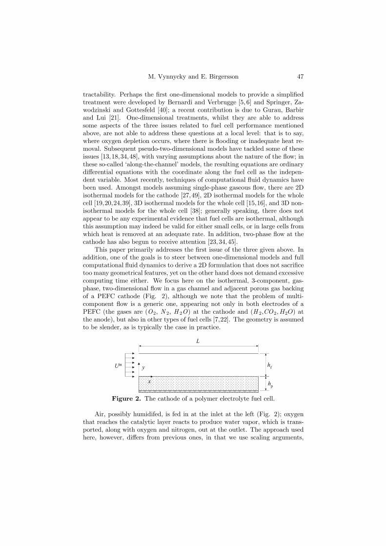
M. Vynnycky and E. Birgersson 47
tractability. Perhaps the first one-dimensional models to provide a simplifiedtreatment were developed by Bernardi and Verbrugge [5, 6] and Springer, Za-wodzinski and Gottesfeld [40]; a recent contribution is due to Gurau, Barbirand Lui [21]. One-dimensional treatments, whilst they are able to addresssome aspects of the three issues related to fuel cell performance mentionedabove, are not able to address these questions at a local level: that is to say,where oxygen depletion occurs, where there is flooding or inadequate heat re-moval. Subsequent pseudo-two-dimensional models have tackled some of theseissues [13,18,34,48], with varying assumptions about the nature of the flow; inthese so-called ‘along-the-channel’ models, the resulting equations are ordinarydifferential equations with the coordinate along the fuel cell as the indepen-dent variable. Most recently, techniques of computational fluid dynamics havebeen used. Amongst models assuming single-phase gaseous flow, there are 2Disothermal models for the cathode [27,49], 2D isothermal models for the wholecell [19,20,24,39], 3D isothermal models for the whole cell [15,16], and 3D non-isothermal models for the whole cell [38]; generally speaking, there does notappear to be any experimental evidence that fuel cells are isothermal, althoughthis assumption may indeed be valid for either small cells, or in large cells fromwhich heat is removed at an adequate rate. In addition, two-phase flow at thecathode has also begun to receive attention [23,34,45].
This paper primarily addresses the first issue of the three given above. Inaddition, one of the goals is to steer between one-dimensional models and fullcomputational fluid dynamics to derive a 2D formulation that does not sacrificetoo many geometrical features, yet on the other hand does not demand excessivecomputing time either. We focus here on the isothermal, 3-component, gas-phase, two-dimensional flow in a gas channel and adjacent porous gas backingof a PEFC cathode (Fig. 2), although we note that the problem of multi-component flow is a generic one, appearing not only in both electrodes of aPEFC (the gases are (O2, N 2, H 2O) at the cathode and (H 2,CO2,H2O) atthe anode), but also in other types of fuel cells [7,22]. The geometry is assumedto be slender, as is typically the case in practice.
hf
hp
L
y
x
Uin
Figure 2. The cathode of a polymer electrolyte fuel cell.
Air, possibly humidifed, is fed in at the inlet at the left (Fig. 2); oxygenthat reaches the catalytic layer reacts to produce water vapor, which is trans-ported, along with oxygen and nitrogen, out at the outlet. The approach usedhere, however, differs from previous ones, in that we use scaling arguments,

48 Analysis of a model for the cathode of a PEFC
nondimensionalization and asymptotics to identify the main governing para-meters and, subsequently, to obtain a reduced model. The benefits of this arethe availability of closed-form analytical solutions in certain limits, as well as amodel that is cheap to compute away from those limits; this feature is impor-tant from the point of view of extension to fuel cell stacks where transport in asmany as 125 such assemblies may need to be computed (see, e.g. [29—31, 42]).The solution of this benchmark problem is useful from several other points ofview:
• as a basis for later work and comparison when two-phase flow is in-troduced;
• to elucidate features that might not be obvious from simply solvingthe full equations.
Regarding the second point, it is clear from the majority of cathode studies thatthe mole fraction of O2 decreases monotonically along the channel, while themole fraction of H 2O increases, with the two slopes in some way dependent onphysical and operating parameters. Among the results of the present treatmentare closed-form expressions for these in certain limits.
The mathematical model is formulated in Section 2. This consists of mass,momentum and species transport equations, and allows for the possibility ofvarying mixture density, as well as the crossed diffusion of species. A nondimen-sional analysis of the governing equations in Section 3 provides an indication ofthe qualitative features one would expect in a multicomponent flow; there arefound to be similarities with classical lubrication theory, in view of the slen-derness of the geometry, except that the reduced Reynolds number is typicallyO (1) . Furthermore, transport in the porous backing is found, to a reasonableapproximation, to be one-dimensional. In Section 4, the first term in an asymp-totic series in the reduced Reynolds number is derived: at leading order, themole fractions are found to be solely a function of the distance along the fuelcell. Section 5 provides a description of a numerical scheme that is subsequentlyused when the reduced Reynolds number is O (1) ; the scheme is verified in thelubrication theory limit for which closed form solutions can be secured. Section6 presents the results. A novel feature which we demonstrate here is that thetraditional method for evaluating fuel cell performance, namely through the useof polarization curves, can be supplemented by the concept of a ‘polarizationsurface’, whereby the average current density is plotted not as a function ofcell potential, but as a function of two dimensionless parameters which dependon cell potential, channel geometry and inlet velocity; consequently, individualpolarization curves are then paths along a ‘polarization surface’. The implica-tions of these results for a PEFC are also considered, in particular as regardsthe limitations of the formulation with respect to liquid water formation, andconclusions are drawn in Section 7.
M. Vynnycky and E. Birgersson 49
2. Mathematical formulation
2.1. Basics of multicomponent flow. We define the local mass averagevelocity, v, of an n-component gas by
v =
Pni=1 ρiviPni=1 ρi
,
where vi denotes the velocity of species i with respect to stationary coordinateaxes, and ρi is the mass concentration (the mass of species i per unit of volumeof solution). For each component, the mass flux with respect to a coordinatesystem fixed in space is given by
ni = ρωiv + ji, i = 1, .., n,
with
ρ =nXi=1
ρi,
where ωi is the mass fraction of species i, given by ωi = ρi/ρ, ji is the massdiffusive flux relative to the mass-averaged velocity, and ρi denotes the densityof species i. If we consider just concentration diffusion for an ideal gas mixture[8], we have
ji =c2
ρ
nXj=1
MiMjDij∇xj , i = 1, .., n; (3)
here (Mi)i=1,..,n are the molecular weights, (Dij)i,j=1,..,n are the multicompo-nent diffusion coefficients, (xi)i=1,..,n is the mole fraction of species i and isgiven by xi = ci/c, where ci is the molar concentration of species i in molesper m3 (ci = ρi/Mi), and
c =nXi=1
ci.
Useful additional identities are c = ρ/M whereM =Pn
i=1 xiMi, and a relationbetween the mass and mole fractions
ωi = xicMi/ρ.
In general, (Dij)i,j=1,..,n are strongly dependent on composition, but can beexpressed in terms of the Stefan-Maxwell diffusion coefficients, (Dij)i,j=1,..,n ,
which are independent of composition. For a 3-component system, as will bethe case here, the relations are of the form [8],
Dij = Dij
½1 +
xk [(Mk/Mj)Dik −Dij ]
xiDjk + xjDik + xkDij
¾, i, j, k = 1, 2, 3 (i 6= j) . (4)
(Dij)i,j=1,..,n can in principle be measured experimentally [8, 41].For the mixture density, we use the constitutive relation for an ideal gas,
ρ =pM
RT, (5)
50 Analysis of a model for the cathode of a PEFC
where p is the pressure, T is the temperature and R is the universal gas con-stant (8.314 kgm2s−2mol-1K−1). We note, in addition, the possibility that themixture viscosity, µmix, will not necessarily be constant either, although wetreat it to be so here.
2.2. Channel. Consider the 2-D steady flow of a 3-component gas in achannel of height hf , adjacent to a porous medium of length L and height hp(see Figure 2). The equations of continuity of mass and momentum for themixture are taken as
∇. (ρv) = 0, (6)
∇. (ρv⊗ v) = −∇µp+
2µ
3∇.v
¶+ µ∇2v− ρgj, (7)
where g is the acceleration due to gravity and j is the unit vector in the positivey-direction; for later use, it is also convenient to define p0, the modified pressure,given by
p0 = p+2
3µ∇.v.
The continuity equation for each of the species,
∇.ni = 0, i = 1, .., 3 (8)
can be recast as, for the cathode of a fuel cell, with n = 3, in the form of twotransport equations
∇.µρv
M
·xO2
xH2O
¸¶= ∇.
µρ
M2M
·∇xO2
∇xH2O
¸¶, (9)
where
M =MN2
µDO2,N2 DO2,N2
DH2O,N2 DH2O,N2
¶−µ
0 MH2ODO2,H2O
MO2DH2O,O2 0
¶.
Here, use has been made of the relation xO2+xN2+xH2O = 1 to eliminate xN2 ,with the diffusion coefficients DO2,H2O, DH2O,O2 ,DH2O,N2 and DO2,N2 givenby (52) .
2.3. Porous backing. For the porous region, volume-averaging of (2.1-2.7) along the lines of DeVidts and White [14] or Whitaker [47] is required. Wepresent this at a moderate level of detail in order to sketch how the transportequations that are normally used, (25) below, can be arrived at; fuller details ofanalogous equations can be found elsewhere [14,47]. First, let B be a quantity(either scalar, vector, or tensor) associated with the gas phase, and let thequantity hBi be the local volume (or superficial) average of B,
hBi ≡ 1
V
ZV(g )
BdV, (10)
and hBi(g) be the intrinsic volume average of B in the gas phase
hBi(g) ≡ 1
V(g)ZV(g )
BdV, (11)

M. Vynnycky and E. Birgersson 51
Also, let γ be the porosity, given by γ = V(g)/V. A comparison of equations(10) and (11) shows that the local and intrinsic volume average for the gasphase is given by
hBi = γ hBi(g) . (12)
Taking the superficial average of (2.4) gives
h∇. (ρv)i = 0, (13)
whilst the superficial average of (2.5) gives (cf. [46])
hvi = −Kµ.³∇ hp0i(g) + hρi(g) gj
´+K.∇2
µhviγ
¶− F. hvi , (14)
where K is the Darcy Law permeability tensor, and F is the Forchheimercorrection tensor. Writing eDij = c2Dij/ρ, we have
∇. hcivi+1
V
ZAgs
cings.vdA+nXj=1
MiMj∇.ÃD eDij
E"∇ hxji+
1
V
ZAgs
xjngsdA
#!
+1
V
nXj=1
MiMjeDij
ZAgs
ngs.∇xjdA = 0, (15)
where ngs represents the unit normal vector pointing from the gas phase tothe solid phase, and Ags represents the area of the gas-solid interface containedwithin V. In the absence of surface reactions and zero normal velocity (passivedispersion), this reduces to
∇. hcivi+nXj=1
MiMj∇.ÃD eDij
E"∇ hxji+
1
V
ZAgs
xjngsdA
#!= 0, (16)
and then
∇. hcivi+nXj=1
MiMj∇.ÃeDij
"∇³γ hxji(g)
´+1
V
ZAgs
xjngsdA
#!= 0, (17)
where we have used the fact that eDij changes slowly with temperature andmole fraction within the representative elementary volume in order to be ableto write
∇.D eDij∇xj
E= ∇.
³ eDij h∇xji´. (18)
To ascertain this, we generalise the reasoning given by Whitaker [47], as follows.With
eDij =pDij
RTM
=pDij
RTM
½1 +
xk [(Mk/Mj)Dik −Dij ]
xiDjk + xjDik + xkDij
¾,
52 Analysis of a model for the cathode of a PEFC
we require
lγeDij
∂ eDij
∂p
%hpi(g )
∇ hpi(g) + ∂ eDij
∂T
%hT i(g )
∇ hT i(g) +nXl=1
∂ eDij
∂xl
%hxli(g )
∇ hxli(g)
¿ 1,
where lγ is the pore length scale. Also, for later use, we need to be able tojustify that within the representative elementary volume
∇. hcivi = ∇.³ p
RThxivi
´= ∇.
³ ρ
Mhxivi
´= ∇.
µhρihMi hxivi
¶;
this would be justified if
lγDγ
Ã∂Dγ
∂p
ºhpi(g )
∇ hpi(g) + ∂Dγ
∂T
ºhT i(g )
∇ hT i(g)!¿ 1,
where Dγ = p/RT . Thus, we would require
lγ
Ã∇ hpi(g)
p− ∇ hT i
(g)
T
!¿ 1; (19)
we verify that this relation is indeed satisfied in Section 3.2.Now, decomposing according to
φ = hφi(g) + φ0,
where φ = (xj , cj ,v, ρ) and the primed quantities denote spatial fluctuations,(13) and (17) can be shown to become, respectively,
∇.³hρi(g) hvi
´= −∇. (hρ0v0i) , (20)
∇.Ãγ hρi(g) hxii(g) hvi(g)
hMi(g)
!
+nXj=1
MiMj∇.ÃeDij
"∇³γ hxji(g)
´+1
V
ZAgs
x0jngsdA
#!
−∇.Ãhρi(g)
hMi(g)hv0x0ii
!= 0, (21)
where we again use analysis due to Whitaker [47] (cf. pp. 14-20). To keep theongoing discussion simple, we assume henceforth that γ is constant. Eventually,

M. Vynnycky and E. Birgersson 53
we arrive at
∇.Ãγ hρi(g) hxii(g) hvi(g)
hMi(g)
!+
nXj=1
MiMj∇.³hDeffij + γDhyd
j δij
i∇ hxji(g)
´= 0,
(22)where Deff
ij is an effective diffusivity tensor given by
Deffij = γ eDij
Ã1 +
1
V(g)ZAgs
ngsbgdA
!,
and δij is the Kronecker delta; here, bg is referred to as the closure variable andis found from the so-called closure problem. Dhyd
j is called the hydrodynamicdispersion tensor and is defined by
Dhydj := − hρi
(g)
hMi(g)v0x0j
®(g).
For gas diffusion electrodes, the following is often used [3, 5,6, 49]:
Deffij = eDijγ
32 ;
this would imply Ã1 +
1
V(g)ZAgs
ngsbgdA
!= γ
12 .
For the cathode, with i = O2, N2 andH2O, we have in more expedient form,on assuming the permeability to be isotropic and constant, and neglecting theForchheimer correction term in (14) and dispersion terms in (20) and (21) (seeSection 3.4),
∇.³hρi(g) hvi
´= 0, (23)
hvi = −κµ
³∇ hp0i(g) + hρi(g) gj
´+
κ
γ∇2 hvi , (24)
∇.Ãhρi(g) hvihMi(g)
"hxO2i
(g)
hxH2Oi(g)
#!
= ∇.
γ32 hρi(g)³hMi(g)
´2 hMi(g)"∇ hxO2i
(g)
∇ hxH2Oi(g)
# , (25)
where
hMi(g) = MN2
ÃhDO2,N2i
(g) hDO2,N2i(g)
hDH2O,N2i(g) hDH2O,N2i
(g)
!
−Ã
0 MH2O hDO2,H2Oi(g)
MO2 hDH2O,O2i(g)
0
!,
54 Analysis of a model for the cathode of a PEFC
with
hDiji(g) = Dij
(1 +
hxki(g) [(Mk/Mj)Dik −Dij ]
hxii(g)Djk + hxji(g)Dik + hxki(g)Dij
);
(23)-(25) are then akin to the governing equations for the porous backing usedby most authors, although with more attention having been paid here to thedistinction between intrinsic and superficial variables, the possibility of non-constant diffusion coefficients and the inclusion of crossed diffusion terms.
2.4. Boundary conditions.2.4.1. Inlet, outlet, upper wall, vertical walls. For boundary conditions in
the channel, we prescribe inlet velocity and gas composition at x = 0, 0 ≤ y ≤hf , so that
u = U in, v = 0, xO2 = xinO2, xH2O = xinH2O, (26)
where v = (u, v). At the upper channel wall (0 ≤ x ≤ L, y = hf ), there is noslip, no normal flow and no componental flux, so that
u = v =∂xO2
∂y=
∂xH2O
∂y= 0. (27)
At the outlet at x = L, 0 ≤ y ≤ hf , we have constant pressure and no diffusivecomponental flux, so that
p = pout,∂v
∂x=
∂xO2
∂x=
∂xH2O
∂x= 0. (28)
At the vertical walls of the porous electrode (x = 0, L,−hp ≤ y ≤ 0), weprescribe no normal flow, no tangential shear and no mass flux for the gascomponents, so that
hui = ∂ hvi∂x
=∂ hxO2i
(g)
∂x=
∂ hxH2Oi(g)
∂x= 0, (29)
where hvi = (hui , hvi).2.4.2. Channel/porous backing interface. In addition, matching conditions
are required for the fluid-porous interface at y = 0, 0 ≤ x ≤ L. The conditionsfor continuity of normal velocity and normal stress are given respectively as
v = hvi , (30)
p− µ∂v
∂y= hpi(g) − µeff
∂ hvi∂y
, (31)
where µeff (= µ/γ) is termed the effective viscosity of the porous medium. Theremaining two conditions that are required have been the subject of longstand-ing debate ever since the work of Beavers and Joseph [4]; a recent contributionis due to Jäger and Mikelic [25]. A summary of possible options for the mo-mentum equation is given by Alazmi and Vafai [1], of which the most relevantfor this application, and indeed most consistent in view of our use of the full
M. Vynnycky and E. Birgersson 55
Navier-Stokes equations for the fluid and a Darcy/Brinkman/Forchheimer for-mulation for the porous medium, is one due to Ochoa-Tapia and Whitaker [35]when inertial effects are important:
u = hui , (32)µ
γ
∂ hui∂y− µ
∂u
∂y=
β1µ
κ12
u+ β2ρu2, (33)
respectively. Here, β1 and β2 are O (1) constants which would need to bedetermined experimentally, although it turns out here that the leading orderproblem is dictated more by (32) than by (33) .
Finally, analogous volume-averaging techniques at the interface to thoseused for heat transfer by [36] are required for the mole fraction transport equa-tions. We do not pursue the details, but simply assume the point values forthe mole fractions of O2 and H2O in the channel to be equal to their intrinsicvalues in the porous backing, so that
hxO2i(g)= xO2 , hxH2Oi
(g)= xH2O, at y = 0, (34)
and in addition that the point values for the mole fraction fluxes of O2 andH2O are equal to their superficial values in the porous medium, so that,
nO2.n = hnO2
.ni , nH2O.n = hnH2O.ni ;using (30) and (34) , we arrive at
γ32∂
∂y
"hxO2i
(g)
hxH2Oi(g)
#=
∂
∂y
·xO2
xH2O
¸, (35)
respectively.2.4.3. Catalyst/porous backing interface. At y = −hf , we would expect
hui , hvi , hxO2i(g) and hxH2Oi
(g) to match to their counterparts in the catalyticlayer, although naturally this approach would require us to model the catalystlayer, and then by extension the membrane and the corresponding regions onthe anode side. This has been done to varying degrees by various authors [5,6,15,18—21,24,34,38—40]. An alternative approach, often adopted when the flowfield in the porous backing and gas channels rather than the electrochemistryin the catalyst and the membrane is of interest [27,33,45,49], is to prescribe acurrent density, I, at this interface. Using Faraday’s Law, the superficial massflux of oxygen is given as a function of current density, so that
hnO2 .ni = −MO2I
4F, (36)
where F is the Faraday constant. The corresponding expression for water isthen taken to be
hnH2O.ni =MH2O(1 + 2α)I
2F, (37)
where α is a parameter accounting for the water transport by electro-osmosisin the membrane; typical values encountered in the literature are α =0.3 [45]
56 Analysis of a model for the cathode of a PEFC
and 0.5≤ α ≤ 1.7 [33,48,49]. Furthermore, since nitrogen does not participatein the reaction at the catalyst layer,
hnN2 .ni = 0. (38)
This leads to the following boundary conditions for hvi, hxO2i(g) and hxH2Oi
(g):
hρi(g) hvi = I
4F(2(1 + 2α)MH2O −MO2
) , (39)
and
hρi(g) hvihMi(g)
"hxO2i
(g)
hxH2Oi(g)
#− γ
32 hρi(g)³hMi(g)
´2 M ∂
∂y
"hxO2i
(g)
hxH2Oi(g)
#=
I
4F
·−1
2(1 + 2α)
¸.
(40)
3. Analysis
3.1. Nondimensionalization. Writing
x =x
L, y =
y
L, ev = v
U in, hevi = hvi
U in, ρ =
ρ
[ρ], heρi(g) = hρi(g)
[ρ],
p =p− pout
[ρ] (U in)2 , hpi
(g) =hpi(g) − pout
[ρ] (U in)2 , p0 =
p0 − pout
[ρ] (U in)2 , hp
0i(g) = hp0i(g) − pout
[ρ] (U in)2 ,
eI = I
[I], M =
M
[M ], hMi(g) = hMi(g)
[M ], c =
c
[ρ] / [M ],
Mi =Mi
[M ], i = 1, .., 3, Dij =
Dij
[D], i, j = 1, .., 3, Deff
ij =Deffij
[D], i, j = 1, .., 3,
Re =[ρ]U inL
µ, Sc =
µ
[ρ] [D], Da =
κ
L2, Fr =
U2
gL,
M=M
[M ] [D],DME(g)
=hMi(g)
[M ] [D],
where [ρ] is a density scale, [D] is a diffusion scale, [I] is a current densityscale and [M ] is a molecular weight scale (all to be either determined or spec-ified shortly), and Re, Sc, Da and Fr are the Reynolds, Schmidt, Darcy andFroude numbers, respectively, we drop the tildes and arrive at the followingnondimensionalised forms. For the channel (0 ≤ x ≤ 1, 0 ≤ y ≤ 1),
∇. (ρv) = 0, (41)
∇. (ρv ⊗ v) = −∇µp+
2δ2
3∇.v
¶+ δ2∇2v−Fr−1ρj, (42)
∇.µρv
M
·xO2
xH2O
¸¶=
δ2
Sc∇.µ
ρ
M2M
·∇xO2
∇xH2O
¸¶, (43)

M. Vynnycky and E. Birgersson 57
where δ2 = Re−1, and for the porous medium (0 ≤ x ≤ 1, −hp/L ≤ y ≤ 0),
∇.³hρi(g) hvi
´= 0, (44)
δ2
2hvi = −∇ hp0i(g) + δ2∇2
µhviγ
¶− Fr−1 hρi(g) j,
∇.Ãhρi(g) hvihMi(g)
"hxO2
i(g)
hxH2Oi(g)
#!
=δ2
Sc∇.
γ32
hρi(g)³hMi(g)
´2 hMi(g)"∇ hxO2
i(g)
∇ hxH2Oi(g)
# , (45)
where 2 = Da. The boundary conditions are now
u = 1, v = 0, xO2= xinO2
, xH2O = xinH2O, at x = 0, 0 ≤ y ≤ hf/L; (46)
u = v =∂xO2
∂y=
∂xH2O
∂y= 0, at 0 ≤ x ≤ 1, y = hf/L; (47)
p = 0,∂v
∂x=
∂xO2
∂x=
∂xH2O
∂x= 0, at x = 1, 0 ≤ y ≤ hf/L; (48)
(49)
hui =∂ hvi∂x
=∂ hxO2i
(g)
∂x=
∂ hxH2Oi(g)
∂x= 0, at x = 0, 1, − hp/L ≤ y ≤ 0.
The boundary conditions for 0 ≤ x ≤ 1, y = −hp/L are now:
hui = 0, hρi(g) hvi = Λ½I
4(2(1 + 2α)MH2O −MO2
)
¾, (50)
hρi(g) hvihMi(g)
"hxO2i
(g)
hxH2Oi(g)
#− δ2γ
32 hρi(g)
Sc³hMi(g)
´2 hMi(g) ∂
∂y
"hxO2i
(g)
hxH2Oi(g)
#(51)
=ΛI
4
µ−1
2(1 + 2α)
¶,
where Λ = [I] [M ] /FU in [ρ] . Finally, the boundary conditions along the fluid-porous interface on y = 0 reduce to
v = hvi , (52)
p− δ2∂v
∂y= hpi(g) − δ2
∂ hvi∂y
, (53)
u = hui , (54)1
γ
∂ hui∂y− ∂u
∂y=
µβ1ε
¶u+
µβ2δ2
¶ρu2. (55)
andhxO2i
(g)= xO2 , hxH2Oi
(g)= xH2O, (56)

58 Analysis of a model for the cathode of a PEFC
γ32∂
∂y
"hxO2i
(g)
hxH2Oi(g)
#=
∂
∂y
·xO2
xH2O
¸. (57)
3.2. Parameters. Typically, U in ∼ 1 ms−1, hf ∼ 10−3 m, hp ∼ 3×10⁻⁴m, L ≥ 10−2 m, [I] ∼ 104 Am−2, pout ∼ 1 atm ∼ 105kgm−1s−2, T ∼ 300− 350K, 0.1 ≤ γ ≤ 0.5, 0.3 ≤ α ≤ 1.7, µ ∼ O(10−5) kgm−1s−1. In addition, MO2 =0.032 kgmol−1, MH2O = 0.018 kgmol−1, MN2
= 0.028 kgmol−1, F = 96487Asmol−1, from which we note that Mmin ≤M ≤Mmax, where
Mmin = M |xH2O=1,xO2=0 = 0.018 kgmol−1,
Mmax = M |xH2O=0,xO2=1 = 0.032 kgmol−1.
Further, we use the constitutive relation for an ideal gas in order to obtain thedensity scale [ρ]; with p ∼ pout, we have ρ ∼ 1 kgm−3, so that [ρ] ∼ 1 kgm−3seems appropriate. For [D], we take O
¡10−5
¢m2s−1 from available literature,
e.g. [5,6]. Note also that the relation (19) is satisfied, since the smallest lengthon the macroscale in the porous backing, hp, is still much larger than the scalefor lγ , 10−5 − 10−6m, suggested by the electrochemical literature [17,43].
Thence, for the nondimensional parameters Re, Sc,Da,Fr,Λ, we arrive at
Re ∼ 104, Sc ∼ 1, Da ≤ 10−6, Fr ∼ 1, Λ ≤ 10−2,
so that δ ∼ 10−2 and ≤ 10−3. We note here that some of these parametershave been encountered before in conjunction with the modelling of flow in solidoxide fuel cells [7,11]: in particular, the Reynolds number, Re, which representsthe ratio of inertial to viscous forces, and the product Schmidt ReSc, which isthe ratio of gas flow rate to the rate of diffusion (in fact ReSc in our formulationcorresponds to the parameter Q in [7,11]). Furthermore, the parameter Λ is ameasure of the ratio of the electrochemical flux of oxygen to the gas flow rate,and thus corresponds to the combination E/Q in [7,11]. For compeleteness, wemention that the Froude number, Fr, is the ratio of inertial to gravitationalforces, whereas the Darcy number, Da, is the ratio of the porous mediumpermeability to the square of the length scale of the entire geometry.
3.3. Narrow-gap approximation. Typically, hf/L, hp/L ¿ 1, whichleads us to further rescaling as follows. Writing
X = x, Y =y
σ, U = u, V =
v
σ, hUi = hui , hV i = hvi
σ,
P = p, P 0 = p0, hP i = hpi , hP 0i = hp0i ,
where σ = hf/L, we simplify further by neglecting terms in O (σ) or lower,although we retain for the time being terms which contain multiples of σ and theother dimensionless parameters. We introduce the dimensionless parameters∆,Σ and Ω, given by
∆ = δ2/σ2, Σ = σ2/ε, Ω = Λ/σ,

M. Vynnycky and E. Birgersson 59
and that an alternative expression for ∆ is ∆ =¡Reσ2
¢−1, i.e. the reciprocal
of the reduced Reynolds number. We have now, for the channel,
∂
∂X(ρU) +
∂
∂Y(ρV ) = 0, (58)
ρ
µU∂U
∂X+ V
∂U
∂Y
¶= −∂P
0
∂X+∆
∂2U
∂Y 2, (59)
0 = −∂P0
∂Y, (60)µ
ρU∂
∂X+ ρV
∂
∂Y
¶·1
MxO2
xH2O
¸=∆
Sc
∂
∂Y
µρ
M2M
∂
∂Y
·xO2
xH2O
¸¶, (61)
and for the porous medium,
0 =∂
∂X
³hρi(g) hUi
´+
∂
∂Y
³hρi(g) hV i
´, (62)
hUi = −∆Σ
∂ hP 0i(g)
∂X+
ε
Σγ
∂2 hUi∂Y 2
, (63)
hV i = − 1
∆Σ2∂ hP 0i(g)
∂Y+
ε
Σγ
∂2 hV i∂Y 2
, (64)
µhρi(g) hUi ∂
∂X+ hρi(g) hV i ∂
∂Y
¶Ã1
hMi(g)
"hxO2i
(g)
hxH2Oi(g)
#!
=∆
Sc
∂
∂Y
γ32 hρi(g)³hMi(g)
´2 hMi(g) ∂
∂Y
"hxO2
i(g)
hxH2Oi(g)
# . (65)
Note also that
P 0 = P +O¡δ2¢, hP 0i(g) = hP i(g) +O
¡δ2¢,
and since δ2 ¿ 1, henceforth, we use the actual pressure rather than themodified pressure. In addition, the gravitational terms in (60) and (64) areO¡Fr−1σ
¢and have therefore been dropped. The boundary conditions are:
for 0 ≤ X ≤ 1, Y = 1,
U = V =∂xO2
∂Y=
∂xH2O
∂Y= 0; (66)
for 0 ≤ X ≤ 1, Y = 0,
V = hV i , (67)
P = hP i(g) , (68)
U = hUi , (69)1
γ
∂ hUi∂Y
− ∂U
∂Y=
µβ1σ
ε
¶U +
µβ2σ
δ2
¶ρU2, (70)
hxO2i(g)= xO2 , hxH2Oi
(g)= xH2O, (71)
60 Analysis of a model for the cathode of a PEFC
γ32∂
∂Y
"hxO2i
(g)
hxH2Oi(g)
#=
∂
∂Y
·xO2
xH2O
¸; (72)
for 0 ≤ X ≤ 1, Y = −H (= hp/hf ),
hUi = 0, hρi(g) hV i = Ω½I
4(2(1 + 2α)MH2O −MO2)
¾, (73)
hρi(g) hV ihMi(g)
"hxO2
i(g)
hxH2Oi(g)
#− ∆γ
32 hρi(g)
Sc³hMi(g)
´2 hMi(g) ∂
∂Y
"hxO2
i(g)
hxH2Oi(g)
#
=ΩI
4
·−1
2(1 + 2α)
¸, (74)
The neglect of streamwise diffusion terms will of course imply that not allof the original boundary conditions at X = 0 and 1 in this reduced formulationcan be satisfied and those terms would need to be reinstated for X ∼ O (σ) and1−X ∼ O (σ) . This is beyond the scope of interest here and for a consistentformulation we simply retain
U = 1, xO2 = xinO2, xH2O = xinH2O, at X = 0, 0 ≤ Y ≤ 1; (75)
hUi = ∂ hxO2i(g)
∂X=
∂ hxH2Oi(g)
∂X= 0, at X = 0, −H ≤ Y ≤ 0. (76)
For the initial discussion, we proceed under the assumption that Σ,∆,Ω ∼O (1) ; later, we will require ΩÀ 1 also. Further simplification is now possibleby noting from (63) that hUi = 0 to leading order, which reduces (62) , (64)and (65) still further. Turning to the porous region near Y = 0−, there is noreason a priori to suppose that the porous core flow should satisfy (67)− (70) ;if it did, we would arrive at U = ∂U
∂Y = 0 at Y = 0, and there would be toomany boundary conditions for (U, V, P ) in the channel. Instead, we require aporous boundary layer for which Y ∼ ε
12 , hUi ∼ ε
12 ; writing
Y = ε12 eY , hUi = ε
12
DeUE , hP i(g) = D ePE(g) , hV i = DeV E ,we have, to leading order, in this layer
∂
∂ eY³hρi(g)
DeV E´ = 0, (77)
DeUE =∂2
∂ eY 2
DeUEγ
, (78)
0 = −∂D ePE(g)∂ eY , (79)
subject to the matching conditions as eY −→ −∞

M. Vynnycky and E. Birgersson 61
DeV E −→ hV i (X, 0) ,DeUE −→ 0,
D ePE(g) −→ hP i(g) (X, 0) ,
where
hV i (X, 0) = limY→0−
hV i , hP i(g) (X, 0) = limY→0−
hP i(g) .
At Y = eY = 0, we have
V =DeV E , (80)
P = hP i(g) , (81)
U = ε12
DeUE , (82)
1
γ
∂DeUE∂ eY − ∂U
∂Y=
µβ1σ
ε
¶U +
µβ2σ
δ2
¶ρU2. (83)
These equations are then used in the following order. First, the channel flowis determined with boundary conditions, to leading order,
U = 0, V =DeV E .
This gives P (X) which serves a boundary condition for hP i(g), and finallyDeUE can be computed, the boundary condition for this being, at leading order,simply
∂DeUE∂ eY = γ
µ∂U
∂Y
¶Y=0
at eY = 0.
As for the species equations, no such boundary layer in ε is necessary, with (65)being valid all the way up to Y = 0−. In addition, we note that the leadingorder equations are independent of β1 and β2.
3.4. Further simplifications and observations. Invoking the consti-tutive relation for an ideal gas in dimensionless variables, with
ρ =M+
Ã[ρ]¡U in
¢2pout
!P, hρi(g) = hMi(g)+
Ã[ρ]¡U in
¢2pout
!hP i(g) (84)
for the channel and porous medium respectively, which can be reduced to justρ = M, hρi(g) = hMi(g) , respectively, for the pressures and velocities beingconsidered here. The reduced system of equations is now, for 0 ≤ X ≤ 1,0 ≤ Y ≤ 1,
∂
∂X(ρU) +
∂
∂Y(ρV ) = 0, (85)
ρ
µU∂U
∂X+ V
∂U
∂Y
¶= − dP
dX+∆
∂2U
∂Y 2, (86)

62 Analysis of a model for the cathode of a PEFC
∂
∂X
µU
·xO2
xH2O
¸¶+
∂
∂Y
µV
·xO2
xH2O
¸¶=∆
Sc
∂
∂Y
µM
M∂
∂Y
·xO2
xH2O
¸¶, (87)
for 0 ≤ X ≤ 1, −H ≤ Y ≤ 0,
hρi(g) hV i = Ω
½I
4(2(1 + 2α)MH2O −MO2
)
¾,
hV i = − 1
∆Σ2∂ hP i(g)
∂Y, (88)
hV i"hxO2
i(g)
hxH2Oi(g)
#− ∆γ
32
Sc hMi(g)hMi(g) ∂
∂Y
"hxO2
i(g)
hxH2Oi(g)
#
=ΩI
4
·−1
2(1 + 2α)
¸. (89)
Note here that (88), as well a consideration of the physical parameters, nowhelps to justify neglecting inertia terms between (14) and (24) , as well asdispersion terms in (20) and (21) . First, the Forchheimer correction term (seeWhitaker [46]) will be of the order of magnitude of the Reynolds number, Reγ ,based on lγ , loosely defined by
Reγ =hρi(g) hvi(g) lγ
µ; (90)
it is justified to use hvi(g) for the velocity scale since the foregoing analysisindicates that flow in the porous backing will be unidirectional. Consequently,using (39) ,
Reγ ∼I
4Fµ(2(1 + 2α)MH2O −MO2) lγ ¿ 1,
as required. In addition, considerations based on this length scale provide somejustification for neglecting dispersion effects in the porous backing, as comparedto molecular diffusion. Experimental results for one-dimensional flows (e.g. [2,pp. 606-9]) indicate that dispersion will be negligible if the Peclet number ofmolecular diffusion, Peγ , in the porous medium, defined here by
Peγ =hvi(g) lγ[D]
,
is much smaller than one; using the parameters given in Section 3.2, this indeedturns out to be the case.
The boundary conditions are: for 0 ≤ X ≤ 1, Y = 1,
U = V =∂xO2
∂Y=
∂xH2O
∂Y= 0; (91)
and for X = 0, 0 ≤ Y ≤ 1,U = 1, xO2 = xinO2
, xH2O = xinH2O, at X = 0, 0 ≤ Y ≤ 1; (92)
M. Vynnycky and E. Birgersson 63
no boundary conditions as such prove to be necessary for X = 0, −H ≤ Y ≤ 0since only ordinary differential equations are solved for −H ≤ Y ≤ 0. At Y = 0for 0 ≤ X ≤ 1, porous and fluid quantities are matched through
U = 0, V = hV i , P = hP i , (93)
hxO2i(g) = xO2
, hxH2Oi(g) = xH2O, (94)
γ32∂
∂Y
"hxO2i
(g)
hxH2Oi(g)
#=
∂
∂Y
·xO2
xH2O
¸. (95)
In general, I will not be constant; even more generally, it cannot be de-scribed a priori, but is determined by considering the transport of species inthe catalyst, membrane and the anode side also. However, a common practicein studies which emphasize the investigation of flow in the porous backing andthe gas channel is simply to prescribe a current density as a function of molefraction. For example. if we use the dimensional form of the Tafel law givenby He, Yi and Nguyen [23],
I =aρ
Mexp
µαcFη
RT
¶,
where αc (= 2) is the transfer coefficient of the oxygen reduction reaction (2),η is the overpotential for the oxygen reaction and a
¡= 10−6 Am mol−1
¢is a
constant related to the exchange current density and oxygen reference concen-tration for the oxygen reaction, we obtain the appropriate scale for [I] as
[I] =a [ρ]
[M ]exp
µαcFη
RT
¶; (96)
consequently, in dimensionless form,
I³hρi(g) , hxO2i
(g), hxH2Oi
(g)´=hρi(g) hxO2
i(g)
hMi(g)= hxO2i
(g). (97)
A dimensional quantity of importance for the determination of polarizationcurves is the average current density, Iav, which is then given by
Iav = [I]
Z 1
0
IdX.
This completes the formulation and necessary definitions. As a next step,we consider the possibility of finding analytical soluton in certain parameterranges; an obvious choice, in view of the geometry, would be the lubricationtheory limit
¡∆−1 ¿ 1
¢. The data given in Table 1 for the base case physi-
cal parameters indicates that ∆−1 ∼ O (1). Obviously, taking channels withsmaller aspect ratio, or operating the fuel cell at lower inlet gas velocity wouldreduce ∆−1, motivating us to then consider the lubrication theory limit, sinceit provides qualitatively useful analytical solutions, as well as a quantitativecomparison with our numerical method (see Section 6).
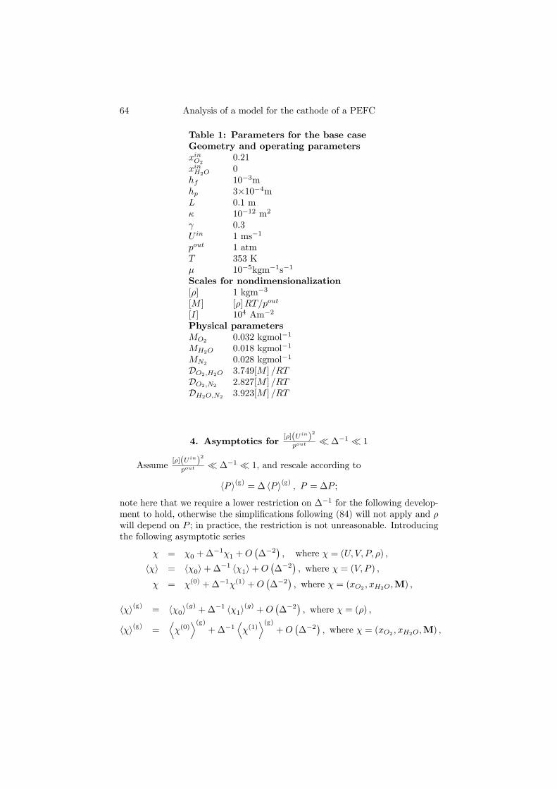
64 Analysis of a model for the cathode of a PEFC
Table 1: Parameters for the base caseGeometry and operating parametersxinO2
0.21xinH2O
0hf 10−3mhp 3×10⁻⁴mL 0.1 mκ 10−12 m2
γ 0.3U in 1 ms−1
pout 1 atmT 353 Kµ 10−5kgm−1s−1
Scales for nondimensionalization[ρ] 1 kgm−3
[M ] [ρ]RT/pout
[I] 104 Am−2
Physical parametersMO2 0.032 kgmol−1
MH2O 0.018 kgmol−1
MN20.028 kgmol−1
DO2,H2O 3.749[M ] /RTDO2,N2 2.827[M ] /RTDH2O,N2 3.923[M ] /RT
4. Asymptotics for[ρ](Uin)2
pout ¿ ∆−1 ¿ 1
Assume[ρ](Uin)
2
pout ¿ ∆−1 ¿ 1, and rescale according to
hP i(g) = ∆ hP i(g) , P = ∆P ;
note here that we require a lower restriction on ∆−1 for the following develop-ment to hold, otherwise the simplifications following (84) will not apply and ρwill depend on P ; in practice, the restriction is not unreasonable. Introducingthe following asymptotic series
χ = χ0 +∆−1χ1 +O
¡∆−2
¢, where χ = (U,V, P, ρ) ,
hχi = hχ0i+∆−1 hχ1i+O¡∆−2
¢, where χ = (V, P ) ,
χ = χ(0) +∆−1χ(1) +O¡∆−2
¢, where χ = (xO2 , xH2O,M) ,
hχi(g) = hχ0i(g)+∆−1 hχ1i
(g)+O
¡∆−2
¢, where χ = (ρ) ,
hχi(g) =Dχ(0)
E(g)+∆−1
Dχ(1)
E(g)+O
¡∆−2
¢, where χ = (xO2 , xH2O,M) ,
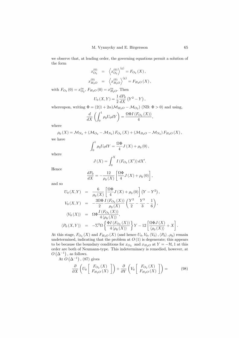
M. Vynnycky and E. Birgersson 65
we observe that, at leading order, the governing equations permit a solution ofthe form
x(0)O2
=Dx(0)O2
E(g)= FO2
(X) ,
x(0)H2O
=Dx(0)H2O
E(g)= FH2O (X) ,
with FO2 (0) = xinO2, FH2O (0) = xinH2O
. Then
U0 (X,Y ) =1
2
dP0dX
¡Y 2 − Y
¢,
whereupon, writing Φ = (2(1 + 2α)MH2O −MO2) (NB: Φ > 0) and using,
d
dX
µZ 1
0
ρ0U0dY
¶=ΩΦI (FO2 (X))
4,
where
ρ0 (X) =MN2 + (MO2 −MN2)FO2 (X) + (MH2O −MN2)FH2O (X) ,
we have Z 1
0
ρ0U0dY =ΩΦ
4J (X) + ρ0 (0) ,
where
J (X) =
Z X
0
I (FO2 (X0)) dX 0.
HencedP0dX
= − 12
ρ0 (X)
·ΩΦ
4J (X) + ρ0 (0)
¸,
and so
U0 (X,Y ) =6
ρ0 (X)
·ΩΦ
4J (X) + ρ0 (0)
¸ ¡Y − Y 2
¢,
V0 (X,Y ) = −3ΩΦ2
I (FO2 (X))
ρ0 (X)
µY 2
2− Y 3
3− 16
¶,
hV0 (X)i = ΩΦI (FO2 (X))
4 hρ0 (X)i,
hP0 (X,Y )i = −Σ2Ω½ΦI (FO2 (X))
4 hρ0 (X)i
¾Y − 12
·ΩΦJ (X)
hρ0 (X)i+X
¸.
At this stage, FO2 (X) and FH2O (X) (and hence U0, V0, hV0i , hP0i , ρ0) remainundetermined, indicating that the problem at O (1) is degenerate; this appearsto be because the boundary conditions for xO2 and xH2O at Y = −H, 1 at thisorder are both of Neumann-type. This indeterminacy is remedied, however, atO¡∆−1
¢, as follows.
At O¡∆−1
¢, (87) gives
∂
∂X
µU0
·FO2 (X)FH2O (X)
¸¶+
∂
∂Y
µV0
·FO2 (X)FH2O (X)
¸¶= (98)

66 Analysis of a model for the cathode of a PEFC
1
Sc
∂
∂Y
ÃM(0)
ρ0 (X)
∂
∂Y
"x(1)O2
x(1)H2O
#!;
for 0 ≤ X ≤ 1, −H ≤ Y ≤ 0,
ΩΦI (FO2 (X))
4 hρ0 (X)i
·FO2 (X)FH2O (X)
¸− γ
32
Sc
M(0)
®(g)hρ0 (X)i
∂
∂Y
Dx(1)O2
E(g)Dx(1)H2O
E(g) = (99)
ΩI (FO2 (X))
4
·−1
2(1 + 2α)
¸.
(98) can be rewritten as
U0
·F 0O2
(X)F 0H2O
(X)
¸+
µ∂U0∂X
+∂V0∂Y
¶·FO2 (X)FH2O (X)
¸=1
Sc
M(0)
ρ0 (X)
∂2
∂Y 2
"x(1)O2
x(1)H2O
#,
and then, on using∂
∂X(ρ0U0) +
∂
∂Y(ρ0V0) = 0,
we have
U0
½·F 0O2
(X)F 0H2O
(X)
¸− 1
ρ0 (X)
∂ρ0∂X
·FO2 (X)FH2O (X)
¸¾=1
Sc
M(0)
ρ0 (X)
∂2
∂Y 2
"x(1)O2
x(1)H2O
#.
Integrating once with respect to Y, we have
λ0 (X)
½·F 0O2
(X)F 0H2O
(X)
¸− 1
ρ0 (X)
∂ρ0∂X
·FO2 (X)FH2O (X)
¸¾µY 2
2− Y 3
3− 16
¶=1
Sc
M(0)
ρ0 (X)
∂
∂Y
"x(1)O2
x(1)H2O
#, (100)
where we have written U0 =λ0(X)ρ0(X)
¡Y − Y 2
¢, with
λ0 (X) = 6
·ΩΦ
4J (X) + ρ0 (0)
¸,
and have already implemented (91) at O¡∆−1
¢. Requiring now, at Y = 0,
γ32∂
∂Y
Dx(1)O2
E(g)Dx(1)H2O
E(g) = ∂
∂Y
"x(1)O2
x(1)H2O
#,
we combine (99) and (100) to give
− 2λ0 (X)
3Ωρ0 (X) I¡F 0O2
(X)¢ ½· F 0O2
(X)F 0H2O
(X)
¸− 1
ρ0 (X)
∂ρ0∂X
·FO2 (X)FH2O (X)
¸¾=
Φ
ρ0 (X)
·FO2 (X)FH2O (X)
¸−·
−12(1 + 2α)
¸.

M. Vynnycky and E. Birgersson 67
Note that this has led to the elimination of x(1)O2and x
(1)H2O
and has instead ledto a pair of non-linear ODEs for FO2
(X) and FH2O (X) .Next, defining
ζO2(X) = FO2 (X) /ρ0 (X) , ζH2O (X) = FH2O (X) /ρ0 (X) ,
we simplify to
−4ΩI (FO2 (X))
·ΩΦ
4J (X) + ρ0 (0)
¸∂
∂X
·ζO2
(X)ζH2O (X)
¸= Φ
·ζO2
(X)ζH2O (X)
¸−·
−12(1 + 2α)
¸,
with initial conditions
ζO2(0) =
xinO2
MN2 + (MO2 −MN2)xinO2+ (MH2O −MN2)x
inH2O
,
ζH2O (0) =xinH2O
MN2 + (MO2 −MN2)xinO2+ (MH2O −MN2)x
inH2O
.
Replacing the partial derivative, we can simplify to
dζO2
dζH2O
=ΦζO2
+ 1
ΦζH2O − 2(1 + 2α),
whence, on applying the inlet conditions,£ΦζO2
(0) + 1¤ζH2O (X)−
£ΦζH2O (0)− 2(1 + 2α)
¤ζO2
(X) = (101)
2(1 + 2α)ζO2(0) + ζH2O (0) .
Note, in addition, that this result holds regardless of the expression used forthe current density.
Returning now to
−4ΩI (FO2 (X))
·Ω
4ΦJ (X) + ρ0 (0)
¸dζO2
dX= ΦζO2
+ 1,
this too can be integrated regardless of the form of I.We have, since J (0) = 0for any current density we care to choose,
ζO2(X) =
1
Φ
½¡ΦζO2
(0) + 1¢µ 4ρ0 (0)
4ρ0 (0) +ΩΦJ (X)
¶− 1¾, (102)
which is effectively an integral equation for ζO2(X) .More convenient is a first-
order ODE for ζO2(X) , which is obtained after rearranging and differentiating,
as
I
µ MN2ζO2(X)
1− (MO2 −MN2) ζO2(X)− (MH2O −MN2) ζH2O (X)
¶= −4ρ0 (0)
Ω
¡ΦζO2
(0) + 1¢¡
ΦζO2(X) + 1
¢2 dζO2
dX,
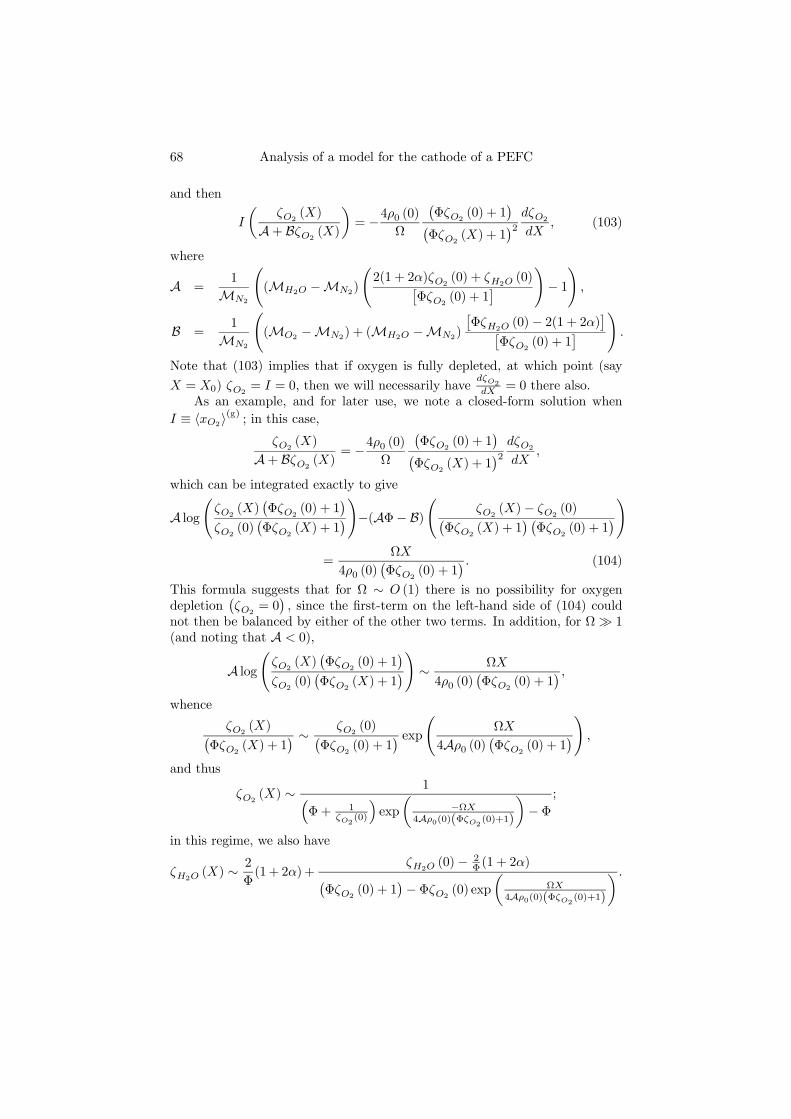
68 Analysis of a model for the cathode of a PEFC
and then
I
µζO2
(X)
A+ BζO2(X)
¶= −4ρ0 (0)
Ω
¡ΦζO2
(0) + 1¢¡
ΦζO2(X) + 1
¢2 dζO2
dX, (103)
where
A =1
MN2
Ã(MH2O −MN2
)
Ã2(1 + 2α)ζO2
(0) + ζH2O (0)£ΦζO2
(0) + 1¤ !
− 1!,
B =1
MN2
Ã(MO2 −MN2) + (MH2O −MN2)
£ΦζH2O (0)− 2(1 + 2α)
¤£ΦζO2
(0) + 1¤ !
.
Note that (103) implies that if oxygen is fully depleted, at which point (say
X = X0) ζO2= I = 0, then we will necessarily have
dζO2dX = 0 there also.
As an example, and for later use, we note a closed-form solution whenI ≡ hxO2i
(g); in this case,
ζO2(X)
A+ BζO2(X)
= −4ρ0 (0)Ω
¡ΦζO2
(0) + 1¢¡
ΦζO2(X) + 1
¢2 dζO2
dX,
which can be integrated exactly to give
A logÃζO2
(X)¡ΦζO2
(0) + 1¢
ζO2(0)¡ΦζO2
(X) + 1¢!−(AΦ− B)Ã ζO2
(X)− ζO2(0)¡
ΦζO2(X) + 1
¢ ¡ΦζO2
(0) + 1¢!
=ΩX
4ρ0 (0)¡ΦζO2
(0) + 1¢ . (104)
This formula suggests that for Ω ∼ O (1) there is no possibility for oxygendepletion
¡ζO2
= 0¢, since the first-term on the left-hand side of (104) could
not then be balanced by either of the other two terms. In addition, for ΩÀ 1(and noting that A < 0),
A logÃζO2
(X)¡ΦζO2
(0) + 1¢
ζO2(0)¡ΦζO2
(X) + 1¢! ∼ ΩX
4ρ0 (0)¡ΦζO2
(0) + 1¢ ,
whence
ζO2(X)¡
ΦζO2(X) + 1
¢ ∼ ζO2(0)¡
ΦζO2(0) + 1
¢ expà ΩX
4Aρ0 (0)¡ΦζO2
(0) + 1¢! ,
and thus
ζO2(X) ∼ 1³
Φ+ 1ζO2 (0)
´exp
µ−ΩX
4Aρ0(0)(ΦζO2 (0)+1)
¶− Φ
;
in this regime, we also have
ζH2O (X) ∼2
Φ(1+ 2α) +
ζH2O (0)−2Φ (1 + 2α)¡
ΦζO2(0) + 1
¢− ΦζO2
(0) exp
µΩX
4Aρ0(0)(ΦζO2 (0)+1)
¶ .

M. Vynnycky and E. Birgersson 69
Note also that, this far, the results are independent of whether or not crosseddiffusion is assumed, or if non-linear diffusion coefficients are used or not.
As a corollary, we observe that the solution at O¡∆−1
¢, i.e. for x(1)O2
,
x(1)H2O
,Dx(1)O2
E(g),Dx(1)H2O
E(g)still remains undetermined, since consideration of
the field equations and boundary conditions at O¡∆−1
¢merely leads to the
solution being fully determined at O (1) . By analogy, to determine the solutionsat O
¡∆−1
¢completely, we would need to consider the field equations and
boundary conditions at O¡∆−2
¢; by this stage, however, the algebra becomes
lengthy and in the interests of brevity we omit further discussion. In fact, onedoes not really gain so much by finding these solutions anyway, since there isno compact solution as there is at O (1), and we proceed instead to a numericalsolution for the general case when ∆−1 ∼ O (1) .
5. Numerical method and results
To complement the asymptotics for ∆−1 ¿ 1, so as to account for regimeswhen ∆−1 ∼ O (1) , the simplified parabolized equations were solved numeri-cally using the Keller-Box discretisation scheme and Newton iteration (see, forexample, Cebeci and Bradshaw [10]). The system of partial differential equa-tions to be solved in the channel is of 8th order, and this is coupled to a 6thorder system of ordinary differential equations in the porous region. As is well-known, the scheme is second-order accurate in both time-like and space-likevariables, and we omit any further details here. As an indication of the speedof the computations, we note that a typical run with 500 points across, and200 points along, the channel required around 100 CPU seconds on a 500 MHzCompaq Alphaserver with 3GB RAM.
Results are presented for the Tafel law given in dimensionless form by (97),and used previously for PEFC studies by [23, 27,33,49]. Throughout, we keepγ = 0.3, T = 353K, and concentrate more on the effect of changes in channelheight and length, porous backing thickness and permeability, pressure, inletspeed and composition. Physically realistic and implementable changes in anyof these will result in, at most, an order of magnitude change in the relevantdimensionless parameter. The most sensitive parameter is Ω, which varies overseveral orders of magnitude as the cell voltage Ecell decreases; note here thatwe revert to using the cell voltage rather than the overpotential, η, with thetwo being related by
Ecell = E0 − η,
where E0(= 1.1V ) is termed the open circuit voltage of the fuel cell.
5.1. Effect of ∆ and Ω. We show first results for Ecell = 0.75V, cor-responding to Ω = 10.2, ranging over several orders of magnitude in ∆, andcompare these with the analytical results in the lubrication theory limit. Fig-ures 3 and 4 are for intrinsic oxygen and water mole fraction at Y = −H,respectively, and demonstrate that the lubrication solution works well for ∆−1
as high as O¡10−2
¢.

70 Analysis of a model for the cathode of a PEFC
0 0.1 0.2 0.3 0.4 0.5 0.6 0.7 0.8 0.9 10
0.05
0.1
0.15
0.2
0.25
X
<xO
2>(g)
∆ =1.89∆ =1.89x101
∆ =1.89x10²
analytical
Figure 3. Comparison of analytical solution for hxO2i(g) at Y = −H with
numerical solutions for ∆ = 1.89, 1.89× 101, 1.89× 10² (Ecell = 0.75V ) .
On the other hand, the base case physical values given in Table 1 corre-spond to ∆ = 1.89. Figure 5 shows the streamwise velocity U at Y = 1
2 , andillustrates the extent of deviation from the classical value 3
2 . An interestinglimit occurs as Ecell is decreased.In this case, Ω increases although the quantity Ω hxO2i
(g) at Y = −H remainsO (1) ; this corresponds to the attainment of the limiting current and the cor-responding plots are given in Figures 6-8; observe that in Figures 6 and 7 thelimiting values for intrinsic oxygen and water mole fraction for the analyticalsolution are reached very rapidly, so that in Figure 6 the curve for hxO2
i(g)effectively lies on the X-axis.

M. Vynnycky and E. Birgersson 71
0 0.1 0.2 0.3 0.4 0.5 0.6 0.7 0.8 0.9 10
0.1
0.2
0.3
0.4
0.5
0.6
X
<xH
2O>(g
)
∆ =1.89∆ =1.89x10 1
∆ =1.89x10 2
analytical
Figure 4. Comparison of analytical solution for hxH2Oi(g) at Y = −H with
numerical solutions for ∆ = 1.89, 1.89× 101, 1.89× 10² (Ecell = 0.75V ) .
0 0.1 0.2 0.3 0.4 0.5 0.6 0.7 0.8 0.9 10
0.5
1
1.5
2
2.5
X
U
∆ =1.89∆ =1.89x10 1
∆ =1.89x10 2
analytical
Figure 5. Comparison of analytical solution for U at Y = 12 with numerical
solutions for ∆ = 1.89, 1.89× 101, 1.89× 10² (Ecell = 0.75V ) .

72 Analysis of a model for the cathode of a PEFC
As regards the numerics, it was found that considerably more outer loop it-erations for the density were required as Ω was increased. For instance, whereas4 iterations sufficed for Ecell = 0.75V, it was common for 20-30 to be necessaryfor Ecell = 0.65V. In addition, there were difficulties in initiating the marchingscheme at X = 0 for higher values of Ω; we surmise this to be due to increasednon-linearity near X=0, since x_O2 changes more abruptly for higher values ofOmega. Whilst setting the channel inlet values as an initial guess for the firststep along the channel was adequate for lower values of Ω, this was found notbe sufficient for Ecell lower than 0.71V ; for those cases, the first-step solutionfor Ecell = 0.71V had to be used instead, then enabling numerical solutions tobe obtained for higher and higher values of Ω until the limiting current wasreached.
0 0.1 0.2 0.3 0.4 0.5 0.6 0.7 0.8 0.9 10
0.1
0.2
0.3
0.4
0.5
0.6
0.7
0.8
0.9
1x 10⁻³
X
<xO
2>(g)
∆ =1.89∆ =1.89x10 1
∆ =1.89x10 2
analytical
Figure 6. Comparison of analytical solution for hxO2i(g) at Y = −H with
numerical solutions for ∆ = 1.89, 1.89× 101, 1.89× 10² (Ecell = 0.65V ) .

M. Vynnycky and E. Birgersson 73
0 0.1 0.2 0.3 0.4 0.5 0.6 0.7 0.8 0.9 10
0.1
0.2
0.3
0.4
0.5
0.6
X
<xH
2O>(g
)
∆ =1.89∆ =1.89x10 1
∆ =1.89x10 2
analytical
Figure 7. Comparison of analytical solution for hxH2Oi(g) at Y = −H with
numerical solutions for ∆ = 1.89, 1.89× 101, 1.89× 10² (Ecell = 0.65V ) .
0 0.1 0.2 0.3 0.4 0.5 0.6 0.7 0.8 0.9 10
0.5
1
1.5
2
2.5
3
3.5
X
U
∆ =1.89∆ =1.89x10 1
∆ =1.89x10 2
analytical
Figure 8. Comparison of analytical solution for U at Y = 12 with numerical
solutions for ∆ = 1.89, 1.89× 101, 1.89× 10² (Ecell = 0.65V ) .

74 Analysis of a model for the cathode of a PEFC
5.2. ‘Polarization surfaces’. It is customary for fuel cell performanceto be given in terms of a polarization curve where the cell potential, Ecell, isgiven as function of the average current density, Iav. Generally speaking, ifthe analysis is done dimensionally, this leads to a vast number of graphs foreach alteration made in one of the physical parameters. However, a majorbenefit of the nondimensional analysis carried out here is that the results canbe expressed considerably more compactly by plotting polarization ‘surfaces’;individual polarization curves will therefore be curves lying on those surfaces.We explain this as follows. From the nondimensionalization given above, theemergent nondimensional parameters were ∆,Σ,Ω and Sc. In addition, thereis γ, which we hold fixed in this study, and xinO2
,xinH2Oand H, whose effect on
fuel cell performance one would like to explore. First, we observe that, in theparameter range of interest, Σ has no effect on Iav, since the dimensionlessdensity is independent of pressure and the pressure in the channel serves asa boundary condition for the pressure in the porous medium. In addition, achange in Sc can only be effected by changes in [ρ] , which only occurs if thecathode is run at a different pressure. Consequently, a tidy representation ofIav is to plot it as a function of ∆ and Ω, for fixed Sc, xinO2
,xinO2and H, the
benefit of this being that the effect of four parameters, hf , L, U in and Ecell, aredisplayed on one graph; since Ω can vary over several orders of magnitude, itproves more convenient to use log (Ω) as a variable. Examples of this are givenbelow.
Figure 9. Polarization surfaces for pout = 1, 3 atm (H = 0.3) .
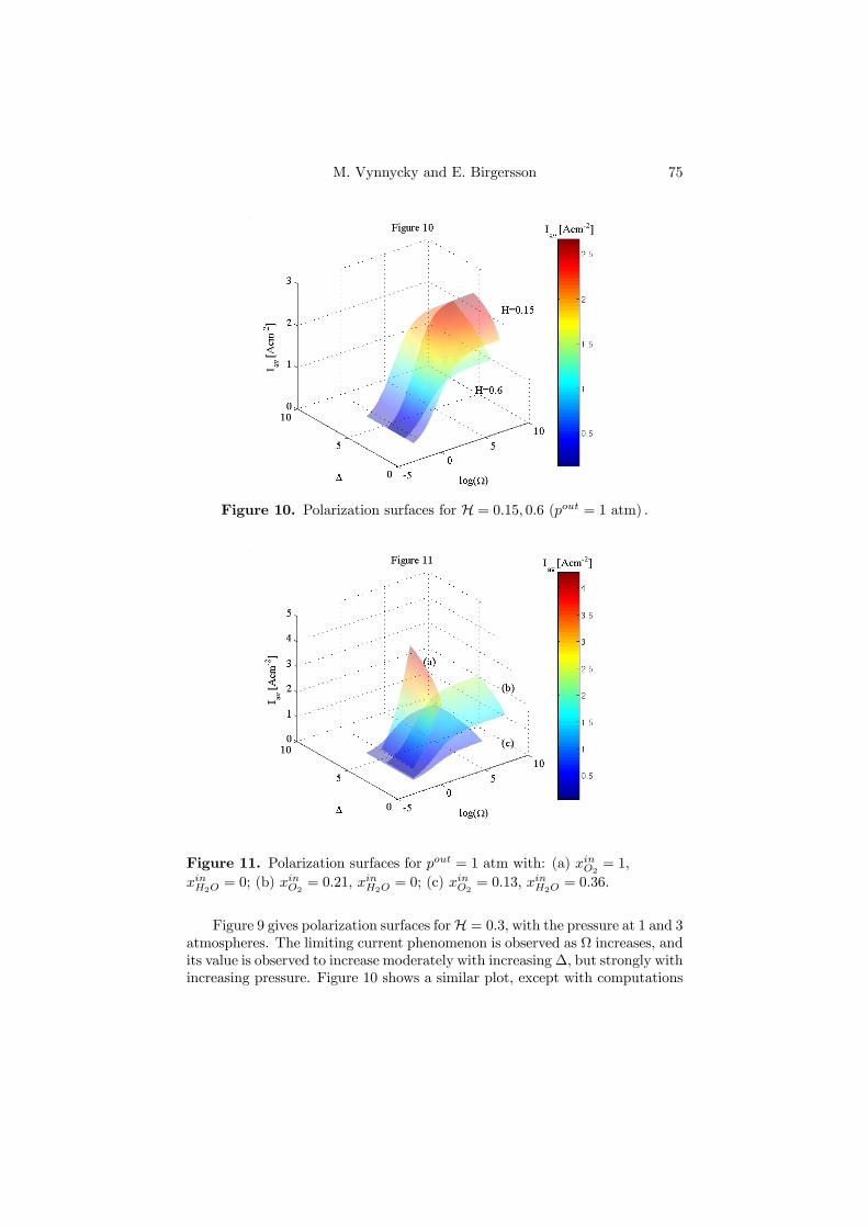
M. Vynnycky and E. Birgersson 75
Figure 10. Polarization surfaces for H = 0.15, 0.6 (pout = 1 atm) .
Figure 11. Polarization surfaces for pout = 1 atm with: (a) xinO2= 1,
xinH2O= 0; (b) xinO2
= 0.21, xinH2O= 0; (c) xinO2
= 0.13, xinH2O= 0.36.
Figure 9 gives polarization surfaces forH = 0.3, with the pressure at 1 and 3atmospheres. The limiting current phenomenon is observed as Ω increases, andits value is observed to increase moderately with increasing∆, but strongly withincreasing pressure. Figure 10 shows a similar plot, except with computations
76 Analysis of a model for the cathode of a PEFC
now for pout = 1 atm, for H = 0.15 and H = 0.6. Average current densitiesare found to be higher for the thinner porous backing, and in both cases alimiting value is evident as Ω is increased. Figure 11 compares the base casefor pout = 1 atm and xinO2
= 0.21 with two other cases at 1 atm which havediffering inlet compositions: dry oxygen
¡xinO2
= 1¢and partially humidified
air, for which xinO2= 0.13 and xinH2O
= 0.36 (corresponding to 76% relativehumidity) [15, 18, 38]. As is evident, increased oxygen content at the inletraises the average current density; for xinO2
= 1, convergence difficulties wereexperienced for quite low values of Ω, which explains the rather narrow rangeof values presented for this case, but nonetheless the average current density ismuch higher than that for the other two cases.
6. Conclusions
In this paper, we have considered a 2-D model for three-component gaseousflow in the cathode of a polymer electrolyte fuel cell. Assuming a slendergeometry, we have derived analytical solutions where possible, and comple-mented these with a numerical study. By choosing to perform the studynondimensionally, we have identified several features that are not evident fromearlier work done dimensionally. In summary, we identify four main dimen-sionless parameters (∆,Ω,Σ, Sc; see Sections 2 and 3 for definitions); otherparameters that are present in this model are the porous backing porosity, γ(held fixed at 0.3 in this study) , the temperature T (held fixed at 353K), theratio of channel and porous backing heights (H), the inlet oxygen and watercontent (xinO2
and xinH2Orespectively) and the number of water molecules affili-
ated to each proton that passes across the membrane to the cathode (α) . Wefind that the flow in the porous backing is essentially unidirectional, althoughit interacts with a fully 2-D flow in the gas channel. Furthermore, Σ is found toplay a secondary role, having next to no effect on the gas mole fraction distri-bution in the porous backing; physically, this implies an insensivity to porousbacking permeability. The fact that the cathode is more or less isobaric givesthat the density is a multiple of the molecular weight. In addition, the Schmidtnumber, Sc, can only be affected by variations in the operating pressure, andwe find that a convenient and compact way to understand fuel cell performanceis to plot average current density as a function of ∆ and Ω for different valuesof Sc and H; this gives a surface which implicitly contains an infinite familyof polarization curves, which is the customary way to assess cell performance.These surfaces have been generated numerically, and in comparatively rapidfashion, using the Keller Box scheme for systems of parabolic partial differen-tial equations, to provide a rather comprehensive parameter study.
The present work was, needless to say, limited in several respects. To beginwith, and has often been stated before, at higher current densities two-phaseflow can be expected as water droplets form at the catalytic layer; this will bethe starting point for future work. Also, we limited ourselves here to prescribingan often-used Tafel law for the current density relation at the catalytic layer, for

M. Vynnycky and E. Birgersson 77
one temperature value and one value of porosity; in addition, α was assumedto be constant along the length of the cell. Naturally, the question arises as towhether more sophisticated modeling would lead to a qualitative change in theresults. Essentially, such an approach would involve attempting to represent thecatalytic layer more faithfully, e.g as has been attempted for molten carbonatefuel cells [37]. A characteristic of this approach would be that a Tafel law isused for reactions across this layer, which would be treated as consisting of thematerial of which the gas-diffusion electrode, as well as polymer electrolyte.Combined with the fact that this layer is much thinner than the gas-diffusionelectrode, it is likely that the functional form for the current density would notbe much different from what we have used here. On the other hand, if theoverpotential and/or temperature are no longer treated as constant, then theexponential term involving these quantities in the expression for the currentdensity could indeed affect the results significantly. Needless to say, this alsois the subject of future work.
Acknowledgment
Financial support from the Swedish Foundation for Strategic Environmen-tal Research (MISTRA) is gratefully acknowledged. The work was done withinthe framework of the Jungner Centre.
Bibliography
[1] B. Alazmi and K. Vafai, Analysis of fluid flow and heat transfer interfacial conditionsbetween a porous layer and a fluid layer, Int. J. Heat and Mass Transfer, 44 (2001) pp.1735-1749.
[2] J. Bear, Dynamics of Fluids in Porous Media, Dover, New York (1988).[3] J. Bear and J. M. Buchlin, Modeling and Applications of Transport Phenomena in
Porous Media, Kluwer Academic Publishers, Boston (1991).[4] G. S. Beavers and D. D. Joseph, Boundary conditions at a naturally permeable wall,
J. Fluid Mech. 30 (1967) pp. 197-207.[5] D. M. Bernardi and M. W. Verbrugge, Mathematical model of a gas diffusion elec-
trode bonded to a polymer electrolyte, AIChE Journal 37 (1991), pp. 1151-1163.[6] D. M. Bernardi and M. W. Verbrugge, A mathematical model of the solid-polymer-
electrolyte fuel cell, J. Electrochem. Soc. 139 (1992), pp. 2477-2491.[7] J. Billingham, A. C. King, R. C. Copcutt and K. Kendall, Analysis of a model for
a loaded, planar, solid oxide fuel cell, SIAM J. Appl. Math., 60 (2000) pp. 574-601.[8] R. B. Bird, W. E. Stewart and E. N. Lightfoot, Transport Phenomena, Wiley, New
York, 1960.[9] E. Birgersson, J. Nordlund, H. Ekström, M. Vynnycky and G. Lindbergh, A
reduced two-dimensional one-phase model for analysis of the anode of a DMFC, J.Electrochem. Soc., 150 (2003) pp. A1368-A1376.
[10] T. Cebeci and P. Bradshaw, Momentum Transfer in Boundary Layers, Washington:Hemisphere Publishing Corporation, 1977.
[11] R. J. Cooper, J. Billingham and A. C. King, Flow and reaction in solid oxide fuelcells, J. Fluid Mech., 411 (2000) pp. 233-262.
[12] E. L. Cussler, Diffusion: Mass Transfer in Fluid Systems, Cambridge University Press,New York, 1984.
[13] K. Dannenberg, P. Ekdunge and G. Lindbergh, Mathematical model of the PEMFC,Journal of Applied Electrochemistry, 30 (2000) pp. 1377-1387.
[14] P. De Vidts and R. E. White, Governing equations for transport in porous electrodes,J. Electrochem. Soc., 144 (1997) pp. 1343-1353.
[15] S. Dutta, S. Shimpalee and J. W. van Zee, Three-dimensional numerical simulationof straight channel PEM cells, Journal of Applied Electrochemistry, 30 (2000) pp. 135-146.
[16] S. Dutta, S. Shimpalee and J. W. van Zee, Numerical prediction of mass exchangebetween cathode and anode channels in a PEM fuel cell, Int. J. Heat and Mass Transfer,44 (2001) pp. 2029-2042.
[17] A. Fischer, J. Jindra and H. Wendt, Porosity and catalyst utilization of thin layercathodes in air operated PEM-fuel cells, J ournal of Applied Electrochemistry, 28 (1998)pp. 277-282.
[18] T. F. Fuller and J. Newman, Water and thermal management in solid-polymer-electrolyte fuel cells, J. Electrochem. Soc. 140 (1993), pp. 1218-1225.
78
M. Vynnycky and E. Birgersson 79
[19] P. Futerko and I-M. Hsing, Two-dimensional finite-element study of the resistance ofmembranes in polymer electrolyte fuel cells, Electrochimica Acta, 45 (2000), pp. 1741-1751.
[20] V. Gurau, H. Liu and S. Kakac, Two-dimensional model for proton exchange mem-brane fuel cells, AIChE Journal, 44 (1998), pp. 2410-2422.
[21] V. Gurau, F. Barbir and H. Liu, An analytical solution of a half-cell model for PEMfuel cells, J. Electrochem. Soc. 147 (2000), pp. 2468-2477.
[22] W. He and Q. Chen, Three-dimensional simulation of a molten carbonate fuel cell stackusing computational fluid dynamics technique, Journal of Power Sources, 55 (1995), pp.25-32.
[23] W. He, J. S. Yi and T. V. Nguyen, Two-phase flow model of the cathode of PEM fuelcells using interdigitated flow fields, AIChE Journal 46 (2000) pp. 2053-2064.
[24] I-M. Hsing and P. Futerko, Two-dimensional simulation of water transport in poly-mer electrolyte fuel cells, Chemical Engineering Science, 55 (2000), pp. 4209-4218.
[25] W. Jäger and A. Mikelic, On the interface boundary condition of Beavers, Joseph,and Saffman, SIAM J. Appl. Math., 60 (2000) pp. 1111-1127.
[26] M. Kaviany, Principles of Heat Transfer in Porous Media, Springer-Verlag, 1991.[27] A. Kazim, H. T. Liu and P. Forges, Modelling of performance of PEM fuel cells
with conventional and interdigitated flow fields, Journal of Applied Electrochemistry 29(1999), pp. 1409-1416.
[28] A. C. King, J. Billingham and R. J. Cooper, Performance modelling of solid oxidefuel cells, Combustion theory and modelling, 5 (2001) pp. 639-667.
[29] J. H. Lee, T. R. Lalk and A. J. Appleby, Modeling electrochemical performance inlarge scale proton exchange membrane fuel cell stacks, Journal of Power Sources, 70(1998) pp. 258-268.
[30] J. H. Lee and T. R. Lalk, Modeling fuel cell stack systems, Journal of Power Sources,73 (1998) pp. 229-241.
[31] G. Maggio, V. Recupero and C. Mantegaza, Modelling of temperature distributionin a solid polymer electrolyte fuel cell stack, Journal of Power Sources, 62 (1996) pp.167-174.
[32] M. J. Morgan and H. N. Shapiro, Fundamentals of Engineering Thermodynamics,Wiley, New York, 1993.
[33] T. V. Nguyen, Modeling two-phase flow in the porous electrodes of proton exchangemembrane fuel cells using the interdigitated flow fields, Electrochemical Society Pro-ceedings, 99-14 (2000) pp. 222-241.
[34] T. V. Nguyen and R. E. White, A water and heat management model for proton-exchange-membrane fuel cells, J. Electrochem. Soc. 140 (1993), pp. 2178-2186.
[35] J. A. Ochoa-Tapia and S. Whitaker, Momentum jump condition at the boundarybetween a porous medium and a homogeneous fluid: inertial effects, J. Porous Media, 1(1998) pp. 201-217.
[36] J. A. Ochoa-Tapia and S. Whitaker, Heat transfer at the boundary between a porousmedium and a homogeneous fluid: the one-equation model, J. Porous Media, 1 (1998)pp. 31-46.
[37] J. A. Prins-Jansen, J. D. Fehribach, K. Hemmes and J. H. W. deWit, A three-phasehomogeneous model for porous electrodes in molten-carbonate fuel cells, J. Electrochem.Soc. 143 (1996), pp. 1617-1628.
[38] S. Shimpalee and S. Dutta, Numerical prediction of temperature distribution in PEMfuel cells, Numerical Heat Transfer, Part A, 38 (2000), pp. 111-128.
[39] D. Singh, D. M. Lu and N. Djilali, A two-dimensional analysis of mass transport inproton exchange membrane fuel cells, International Journal of Engineering Science 37(1999), pp. 431-452.
[40] T. E. Springer, T. A. Zawodzinski and S. Gottesfeld, Polymer electrolyte fuel cellmodel, J. Electrochem. Soc. 138 (1991), pp. 2334-2342.
[41] R. Taylor and R. Krishna, Multicomponent Mass Transfer, Wiley, New York, 1993.
80 Analysis of a model for the cathode of a PEFC
[42] D. Thirumalai and R. E. White, Mathematical modeling of proton-exchange-membrane fuel-cell stacks, J. Electrochem. Soc. 144 (1997), pp. 1717-1723.
[43] M. Uchida, Y. Fukuoka, Y. Sugawara, N. Eda and A. Ohta, Effects of mictrostruc-ture of carbon support in the catalyst layer on the performance of polymer-electrolytefuel cells, J. Electrochem. Soc. 143 (1996), pp. 2245-2252.
[44] M. W. Verbrugge and R. F. Hill, Transport phenomena in perfluorosulfonic acidmembranes during the passage of a current, J. Electrochem. Soc. 137 (1990), pp. 1131-1138.
[45] Z. H. Wang, C. Y. Wang and K. S. Chen, Two-phase flow and transport in the aircathode of proton exchange membrane fuel cells, Journal of Power Sources, 94 (2001)pp. 40-50.
[46] S. Whitaker, The Forchheimer equation: a theoretical development, Transport inPorous Media, 25 (1996) pp. 27-61.
[47] S. Whitaker, The method of volume averaging, Kluwer, Dordrecht, 1999.[48] J. S. Yi and T. V. Nguyen, An along-the-channel model for proton exchange membrane
fuel cells, J. Electrochem. Soc. 145 (1998), pp. 1149-1159.[49] J. S. Yi and T. V. Nguyen, Multicomponent transport in porous electrodes of proton
exchange membrane fuel cells using the interdigitated gas distributors, J. Electrochem.Soc. 146 (1999), pp. 38-45.

Paper 2


A quantitative study of the effect offlow-distributor geometry in the cathode of a
PEM fuel cellErik Birgersson and Michael Vynnycky
Department of Mechanics, FaxénLaboratoriet, KTH,SE-100 44, Stockholm, Sweden
Abstract. An isothermal three-dimensional model describing mass, momentumand species transfer in the cathode of a proton exchange membrane fuel cell has beenused to study four different flow distributors: interdigitated, coflow and counterflowchannels, and a foam. A quantitative comparison of the results shows that the inter-digitated channels can sustain the highest current densities, followed in descendingorder by the foam, the counterflow and the coflow channels. The foam yields the mostuniform current density distribution at higher currents, but also induces the greatestpressure drop.
1. Introduction
In view of ever increasing levels of environmental pollution and thus adesire to replace the fossil-fuel-based economy with a cleaner alternative, thefuel cell has in recent years become a prime candidate as a power source fortransport and stationary applications. The potential use of fuel cells rangesfrom distributed power sources and portable applications, such as laptops [1]or even for the future dismounted soldier [2], to vehicles.
One such type of cell is the proton exchange membrane fuel cell (PEMFC),a schematic representation of which is shown in figure 1. The basic cell consistsof two porous electrodes, termed the anode and the cathode, separated by aproton conducting membrane. The porous electrodes are made of a compositematerial, containing carbon cloth and a hydrophobic agent, such as polyte-trafluorethylene. Each electrode has a thin layer containing an electrocatalyst,such as platinum, that is dispersed on the carbon cloth and is in contact withthe membrane, usually a hydrated perfluorinated sulfonic acid polymer. In ad-dition a bipolar plate, essentially graphite into which flow and cooling channelshave been machined, is situated adjacent to each electrode. In the course ofoperation, an oxidant, usually oxygen from air which is either dry or humidifiedto some extent, is fed at the inlet on the cathode side and transported to theelectrolyte/cathode interface; the fuel on the other hand, normally hydrogen,is fed at the anode inlet and is transported to the electrolyte/anode interface.The reactions occurring at these interfaces are then
2H2 → 4H+ + 4e− at the anode, (1)
O2 + 4H+ + 4e− → 2H2O at the cathode, (2)
which are termed the hydrogen oxidation reaction (HOR) and the oxygen re-duction reaction (ORR), respectively. Thus, the protons produced at the anode

84 A study of flow-distributors in the cathode of a PEFC
are transported through the membrane to the cathode, whilst the electrons candrive a load through an external circuit.
Bipolar platewith flow fieldand coolingchannels
CathodeAnode +-
Agglomeratenucleus
e-
Carbon particlewith catalyst
Polytetrafluorethylene(PTFE)
Carbon cloth
MembranePorousbacking
Porousbacking
Active layers
H2H2O
O2N2H2O
Polymer electrolyte,e.g. Nafion andliquid water
Agglomerate
Flowfield
Coolingchannels
Figure 1. Schematic of a polymer electrolyte fuel cell.
During recent years, a number of mathematical models have been developed inan attempt to understand the phenomena occurring in a PEM fuel cell. Sincea complete fuel cell model would have to address mass, momentum, speciesand heat transfer in gas and liquid phases in a three-dimensional geometry,as well as the electrokinetics for the ORR and HOR, most models choose tofocus on only some of these aspects at a time. The first models to appear wereone-dimensional followed by two-dimensional, see [3] for a list of these models;lately three-dimensional models, based on computational fluid dynamics, havealso begun to appear [4-8]. Dutta, Shimpalee and van Zee considered firsta straight channel flow under isothermal conditions [4], followed later by amodel for flow in a serpentine channel [5]; most recent work extends [4] totake into account heat transfer for a straight channel flow [6]. Costamagnaconsiders non-isothermal conditions and treats the flow distributor as a porousmaterial [7]. Berning [8] introduces a non-isothermal two-phase model for astraight channel, with a simplified two-phase treatment in the porous backings,neglecting the interaction between the liquid and gaseous phase and assumingone-phase flow in the flow channel. However, none of the above consider in aquantitative and comparative way the effect of flow distributor geometry onfuel cell performance.

E. Birgersson and M. Vynnycky 85
To extend the work on three-dimensional modelling, we have conducted aquantitative comparison of the performance of four common flow distributors:parallel channels, run in both coflow and counterflow, interdigitated channelsand a porous distributor, such as a foam. To limit the computational require-ments, we assume that the anode side is run at such conditions that it is ableto fully sustain any current created at the cathode, i.e. a fully moisturizedanode that is run at high stoichiometry. In addition, we assume that sufficientcooling is provided to keep the cathode isothermal, a not unreasonable prelim-inary assumption in view of the temperature distributions obtained by [6, 8],which show that the temperature only varies by a couple of degrees in the cath-ode. These assumptions enable us then to consider isothermal, 3-component,gas-phase, three-dimensional laminar flow in the flow distributor and adjacentporous backing on the cathode side only.
The mathematical model, consisting of mass, momentum and species trans-port equations, as well as the geometries of the flow distributors considered, areintroduced in Section 2. We focus also on how a rather detailed agglomeratemodel for the electrochemical aspects of the active layer, derived by [9], canbe simply implemented into the present formulation. Details of the numericalsolver used, CFX-4.4 [10], followed by its verification against an asymptotic so-lution obtained previously [3], are given in Section 3. The results from differentflow distributors are then compared and discussed in Section 4. We finish withconclusions in Section 5.
2. Model description
2.1. Flow-distributor geometry. The electrochemical reactions thatoccur at the active layers depend on a sufficiently fast transport of reactants to,and products away from, the active sites so as to limit concentration overpoten-tials. Towards this end, the bipolar plates contain grooved channels, which cantake a number of different shapes. Amongst the most common designs todayare:
(a): parallel channels, with only one pass over the porous backing, runin coflow, as shown in figure 2a.
(b): parallel channels, with only one pass over the porous backing, runin counterflow, as shown in figure 2a.
(c): interdigitated channels, where channels are terminated, in order toforce the flow into the porous backing, see figure 2b.
(d): a porous material, such as a foam; here, the entire surface of theporous backing is in contact with the gas flow, see figure 2c, in contrastto the channel based flow distributors, which contain ‘dead’ zonesbetween the channels.
(e): serpentine flow channels, comprising one long channel with manypasses over the porous backing.
(f): a combination of some of the above, e.g. (a) and (e), (b) and (e).
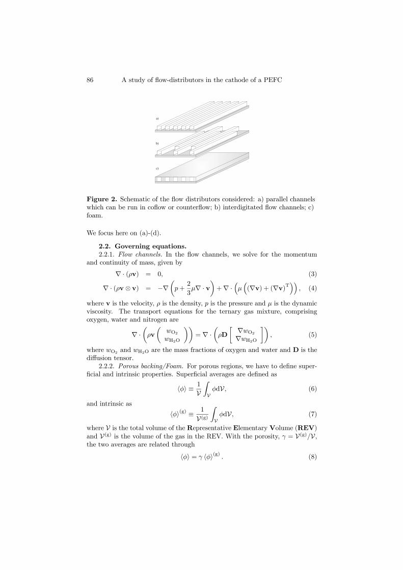
86 A study of flow-distributors in the cathode of a PEFC
a)
b)
c)
Figure 2. Schematic of the flow distributors considered: a) parallel channelswhich can be run in coflow or counterflow; b) interdigitated flow channels; c)foam.
We focus here on (a)-(d).
2.2. Governing equations.2.2.1. Flow channels. In the flow channels, we solve for the momentum
and continuity of mass, given by
∇ · (ρv) = 0, (3)
∇ · (ρv⊗ v) = −∇µp+
2
3µ∇ · v
¶+∇ ·
³µ³(∇v) + (∇v)T
´´, (4)
where v is the velocity, ρ is the density, p is the pressure and µ is the dynamicviscosity. The transport equations for the ternary gas mixture, comprisingoxygen, water and nitrogen are
∇ ·µρv
µwO2
wH2O
¶¶= ∇ ·
µρD
·∇wO2
∇wH2O
¸¶, (5)
where wO2and wH2O are the mass fractions of oxygen and water and D is the
diffusion tensor.2.2.2. Porous backing/Foam. For porous regions, we have to define super-
ficial and intrinsic properties. Superficial averages are defined as
hφi ≡ 1
V
ZVφdV, (6)
and intrinsic as
hφi(g) ≡ 1
V(g)ZVφdV, (7)
where V is the total volume of the Representative Elementary Volume (REV)and V(g) is the volume of the gas in the REV. With the porosity, γ = V(g)/V,the two averages are related through
hφi = γ hφi(g) . (8)

E. Birgersson and M. Vynnycky 87
Conservation of mass and momentum is given respectively by
∇ ·³hρi(g) hvi
´= 0, (9)
∇ ·³hρi(g) hvi⊗ hvi
´+ µK−1 · hvi = −∇
µhpi(g) + 2
3
µ
γ∇ · hvi
¶+∇ ·
µµ
γ
³∇ hvi+ (∇ hvi)T
´¶, (10)
where K is the permeability tensor.The species transport equations are described by
∇ ·Ãhρi(g) hvi
ÃhwO2i
(g)
hwH2Oi(g)
!!= ∇ ·
Ãhρi(g) γ hDi(g)
"∇ hwO2i
(g)
∇ hwH2Oi(g)
#!,
(11)where hDi(g) is the total mass diffusion tensor, containing contributions froman intrinsic effective mass diffusion tensor and an intrinsic hydrodynamic dis-persion tensor. For a more detailed discussion of these, see [3].
2.3. Boundary conditions.2.3.1. Inlet. At the inlet, we prescribe the normal velocity and the gas
composition for the channel distributors:
v · ex = U in, v · ey = v · ez = 0, wO2 = winO2, wH2O = winH2O; (12)
in addition, for the counterflow distributor, we require
v · ex = −U in, v · ey = v · ez = 0, wO2 = winO2, wH2O = winH2O, (13)
for the second channel (see figure 3b);For the foam:
hvi · ex = U in, hvi · ey = hvi · ez = 0, hwO2i(g)= winO2
, hwH2Oi(g)= winH2O.
(14)2.3.2. Outlet. At the outlet, we specify the pressure and the streamwise
gradients of the velocities and species are set to zero, corresponding to fullydeveloped flow conditions. For the channels:
p = pout, (15)
(ex ·∇) (v · ey) = 0, (16)
(ex ·∇) (v · ez) = 0, (17)
ex ·∇wO2 = ex ·∇wH2O = 0; (18)
correspondingly, for the foam:
hpi(g) = pout, (19)
(ex ·∇) (hvi ·ey) = 0, (20)
(ex ·∇) (hvi ·ez) = 0, (21)
ex ·∇ hwO2i(g) = ex ·∇ hwH2Oi
(g) = 0. (22)

88 A study of flow-distributors in the cathode of a PEFC
2.3.3. Walls. At the walls of the channels, we specify no-slip, no normalflow and no componental flux:
v = 0, (23)
n ·∇wO2= n ·∇wH2O = 0, (24)
where n is the unit normal to a wall. In the porous backing and foam, zeroshear stress, no normal flow and no componental flux conditions are applied;these are, respectively,
(n ·∇) (hvi ·t) = 0, (25)
n · hvi = 0, (26)
n ·∇ hwO2i(g) = n ·∇ hwH2Oi
(g) = 0, (27)
where t is the unit tangent to a wall.2.3.4. Symmetry conditions. The flow distributors considered in this pa-
per are all of periodic character, see figure 2, allowing us to reduce the com-putational domain for each by introducing unit cells, see figure 3, with theappropriate symmetry conditions. For the foam and porous backing:
(n ·∇) (hvi ·t) = 0, (28)
n · hvi = 0, (29)
n ·∇ hwO2i(g) = n ·∇ hwH2Oi
(g) = 0; (30)
correspondingly, for the channels:
(n ·∇) (v · t) = 0, (31)
n · v = 0, (32)
n ·∇wO2= n ·∇wH2O = 0. (33)
2.3.5. Channel/porous backing interface. At the interface between the porousbacking and the flow channels, we couple the point wise velocities, normal andshear stresses in the plain fluid (flow channels) with their superficial counter-parts in the porous medium. The mass fractions and fluxes of oxygen and waterare continuous across the interface.
2.3.6. Active region/porous backing interface. The active region in the cath-ode is sufficiently thin to allow us to treat it as a boundary condition for theporous backing. Using Faraday’s Law, the mass fluxes of oxygen and water canbe found as
hnO2i · ey = −MO2 hii · ey4F
, (34)
hnH2Oi · ey =(1 + 2α)MH2O hii · ey
2F, (35)
where hnO2i and hnH2Oi are the mass fluxes, α is the amount of water draggedthrough the membrane with each proton,Mi is the molecular mass of species i,hii is the superficial current density and F is Faraday’s constant. The superficial
E. Birgersson and M. Vynnycky 89
velocity from the reaction can be derived from the the theory of multicompo-nent mass transfer as
hρi(g) hvi · ey=hii · ey4F
((2 + 4α)MH2O −MO2) . (36)
2.4. Constitutive relations. Assuming an ideal gas, the gas density canbe found from
ρ =pM
RT, (37)
where M = (wO2/MO2 + wH2O/MH2O + wN2/MN2)−1 is the mean molecular
mass, R is the universal gas constant and T is the temperature. The massfraction of nitrogen is given by
wN2 = 1− wO2 − wH2O. (38)
We note here that the molar fractions xi are related to the mass fractions wiby
xi =wiM
Mi. (39)
Furthermore, in the most general case, the dynamic viscosity, µ, is also a func-tion of the composition, but for simplicity it is considered constant in thispaper. The corresponding constitutive properties in the porous backing andfoam are the same, but based on intrinsic values.
An expression for the diffusion tensor [11] can be found from the diffusioncoefficients eDij for the molar diffusion flux, relative to a molar-averaged velocityframe, as eD11 = DO2,N2(xO2DH2O,N2 + (1− xO2)DO2,H2O)/S, (40)eD12 = xO2DH2O,N2(DO2,N2 −DO2,H2O)/S, (41)eD21 = xH2ODO2,N2(DH2O,N2 −DO2,H2O)/S, (42)eD22 = DH2O,N2(xH2ODO2,N2 + (1− xH2O)DO2,H2O)/S, (43)
S = xO2DH2O,N2 + xH2ODO2,N2 + xN2DO2,H2O, (44)
where Dij are the binary Maxwell-Stefan diffusion coefficients. Since we usethe mass diffusion flux relative to the mass-averaged velocity, the followingtransformation is required:
D = BWX−1 eDXW−1B−1, (45)
B = δij − wi
µ1− wnxj
xnwj
¶, i, j = 1, 2, n = 3, (46)
X = xiδij, i, j = 1, 2, (47)
W = wiδij, i, j = 1, 2, (48)
where δij is the Kronecker delta. The binary Maxwell-Stefan diffusion coeffi-cients are corrected for pressure and temperature via
Dij(T, p) =p0p
µT
T0
¶ 32
Dij(T0, p0), (49)
90 A study of flow-distributors in the cathode of a PEFC
stemming from kinetic gas theory [12]. The cross terms in the diffusion tensorD are around one to two orders of magnitude lower for the operating parametersin this study than the diagonal terms, allowing us to neglect their contributions,whence
D =
·D11 00 D22
¸. (50)
In the porous media, i.e. in the foam and porous backing, we apply a Brugge-man correlation for the superficial effective mass diffusion tensor
hDi = γ32D. (51)
The permeabilities of the porous backing and foam are taken to be isotropic
K = κδij, (52)
where κ is the permeability.
2.5. Electrokinetics and the active layer. An expression is still re-quired for the current density hii ·ey given in equation (36) . A novel feature ofthis paper is to implement an expression from an agglomerate model derived byJaouen et al. [9], and subsequently validated experimentally [13]. Although [9]considers an active layer of finite thickness, it is possible to demonstrate that,for our purposes, the active layer need not be resolved explicitly, but rathercan be treated implicitly as a boundary condition. Some further details are asfollows.
The volumetric current density hivi, given by [9], is approximated as
hivi = Ai0¡1− γpol
¢(1− γa) exp
µ−αrFRT
η
¶FhcO2i
(g)
crefO2
(53)
where Ai0 is the volumetric exchange current density in the agglomerates, γpolis the volume fraction of the polymer electrolyte in the agglomerate nucleus,hcO2i
(g) = hwO2i(g) hρi(g) /MO2 is the molar concentration of oxygen, αr is the
cathodic transfer coefficient for the ORR, n is the number of electrons consumedin the ORR per oxygen molecule, η is the overpotential at the cathode (definednegative), and γa is the volume fraction of pores in the active layer. F is thenucleus effectiveness factor, defined as
F =3
Υr
µ1
tanh(Υr)− 1
Υr
¶, (54)
with Υ given by
Υ =
sAi0
¡1− γpol
¢exp
¡−αrF
RT η¢
nFD, (55)
where D is an effective oxygen permeability in the agglomerates and r is the ra-dius of the agglomerate nucleus. This agglomerate model was validated by [13]for a small PEM fuel cell with an area of 2 cm2 at conditions well above the sto-ichiometric flow rate, allowing the cell there to be modelled one-dimensionally,since concentration gradients in the streamwise direction in the cathode can
E. Birgersson and M. Vynnycky 91
be neglected. In this paper, however, the aim is to capture and study two-and three-dimensional effects. The one-dimensional agglomerate model can beused for this purpose by noting that the geometry of the active layer studied isslender, i.e. its thickness, ha, is much smaller than its width (w) and breadth(L) , implying that only gradients in the normal direction in the active layerwill contribute to mass transfer; consequently, this allows us to treat the activelayer locally as one-dimensional. Although we omit the details here, it is pos-sible to show by scale analysis that we will not have any gradients of oxygenin the normal direction in the active layer, since the magnitude of the diffusioncoefficient in the agglomerates is O(10−11) m2s−1, as compared to O(10−5)m2s−1 in the pores. The additional approximation of reducing the active layerto a boundary condition corresponds to an infinite effective proton conductiv-ity in the the active layer. The total current density is then given locally byhii · ey = hii = hiviha.
Jaouen et al. [9] discerned four different regimes, where the Tafel slope dou-bles or even quadruples, and subsequently supplied the experimental validationto support these [13]. In regime 1, the active layer is controlled by Tafel kineticsand is first order in the oxygen concentration. Regime 2 displays a doublingof the Tafel slope, due to the active layer being governed by Tafel kinetics andoxygen diffusion in the agglomerates, but still remains first order in the oxygenconcentration. A doubling of the Tafel slope is observed in the third regime,where the active layer is controlled by the Tafel kinetics, in addition to protonmigration. The oxygen dependence here is half-order. The final regime, thefourth, shows a quadrupling of the Tafel slope, and is attributable to an activelayer controlled by Tafel kinetics, proton migration and oxygen diffusion in theagglomerates. The oxygen dependence is half-order, as in regime 3.
By assuming that we have no resistance to proton migration, we limit thevalidity of the expression to regimes 1 and 2, i.e. to an active layer controlledby Tafel kinetics at low overpotentials, and at higher overpotentials by Tafelkinetics coupled with oxygen diffusion resistance in the agglomerates. We arethus able to capture the doubling of the Tafel slope due to mass transfer lim-itations in the agglomerates, although the doubling due to proton migrationresistance and a quadrupling of the slope are not modelled.
Finally, we note that of more use, as regards judging fuel cell performance,than the overpotential, η, is the cell voltage, Ecell, where
η = Ecell −E0, (56)
and E0 is the equilibrium potential.
3. Numerics and verification
A commercial computational fluid dynamics code, CFX-4.4, based on fi-nite volumes, was used to implement the model outlined above. As can be seenin figure 2, all of the flow distributors are periodic in the spanwise direction.Hence, a representative computational unit cell, with symmetry boundary con-ditions on both sides in the spanwise coordinate, can be introduced. The unit

92 A study of flow-distributors in the cathode of a PEFC
cells for the distributors are chosen so that the area of the active layer andthe contact area between the channels and porous backing are the same forall, with the exception of the foam, which covers the entire porous backing asdepicted in figure 3.
a) b)
d)c)
ex
ez
ey
w
w
w/2
w/2
hp hp
hphp
hf hf
hf hf LL
L L
wf
wf
wf
wf
wf
wf
Figure 3. Schematic of the computational unit cells: a) parallel channels runin coflow; b) parallel channels run in counterflow; c) interdigitated channels;d) foam.
Using a structured mesh, each flow distributor with porous backing was resolvedas follows:
(a): parallel channels run in coflow ; the channel contained 104 compu-tational cells and the porous backing 2 × 10⁴ cells, giving a total of3 × 104 cells. Mesh independence was assured by comparing with amesh comprising 1.2 × 10⁵ cells and the difference was found to be∼ 1% for the average current density.
(b): parallel channels run in counterflow ; the two channels with 104
cells each and the porous backing with 4 × 10⁴ cells, giving a totalof 6 × 10⁴ cells. Mesh independence was assured by comparing witha mesh comprising 2 × 10⁵ cells and the difference was found to be∼ 1% for the average current density.
(c): interdigitated channels; the two channels with 104 cells each andthe porous backing with 4× 10⁴, giving a total of 6× 10⁴ cells. Meshindependence was assured by comparing with a mesh comprising2× 105 cells and the difference was found to be ∼ 4% for the averagecurrent density. At higher currents, i.e. hii > 4 Acm−2, more than6× 104 cells were necessary to resolve the flow in the porous backing.We did not pursue these higher current densities, however.
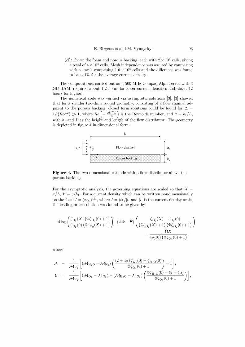
E. Birgersson and M. Vynnycky 93
(d): foam; the foam and porous backing, each with 2× 10⁴ cells, givinga total of 4×10⁴ cells. Mesh independence was assured by comparingwith a mesh comprising 1.6× 10⁵ cells and the difference was foundto be ∼ 1% for the average current density.
The computations, carried out on a 500 MHz Compaq Alphaserver with 3GB RAM, required about 1-2 hours for lower current densities and about 12hours for higher.
The numerical code was verified via asymptotic solutions [3]. [3] showedthat for a slender two-dimensional geometry, consisting of a flow channel ad-jacent to the porous backing, closed form solutions could be found for ∆ =
1/¡Reσ2
¢À 1, where Re
³= ρU inL
µ
´is the Reynolds number, and σ = hf/L,
with hf and L as the height and length of the flow distributor. The geometryis depicted in figure 4 in dimensional form.
hf
hp
L
y
x
Uin Flow channel
Porous backing
Figure 4. The two-dimensional cathode with a flow distributor above theporous backing.
For the asymptotic analysis, the governing equations are scaled so that X =x/L, Y = y/hf . For a current density which can be written nondimensionallyon the form I = hxO2i
(g), where I = hii /[i] and [i] is the current density scale,the leading order solution was found to be given by
A logÃζO2
(X)¡ΦζO2
(0) + 1¢
ζO2(0)¡ΦζO2
(X) + 1¢!−(AΦ− B)Ã ζO2
(X)− ζO2(0)¡
ΦζO2(X) + 1
¢ ¡ΦζO2
(0) + 1¢!
=ΩX
4ρ0(0)¡ΦζO2
(0) + 1¢ ,
where
A =1
MN2
·(MH2O −MN2)
µ(2 + 4α) ζO2
(0) + ζH2O(0)
ΦζO2(0) + 1
¶− 1¸,
B =1
MN2
·(MO2 −MN2) + (MH2O −MN2)
µΦζH2O(0)− (2 + 4α)
ΦζO2(0) + 1
¶¸,
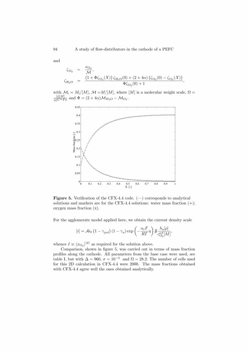
94 A study of flow-distributors in the cathode of a PEFC
and
ζO2=
xO2
M ,
ζH2O =
¡1 +ΦζO2
(X)¢ζH2O(0) + (2 + 4α)
¡ζO2
(0)− ζO2(X)
¢ΦζO2
(0) + 1,
withMi =Mi/[M ],M =M/[M ], where [M ] is a molecular weight scale, Ω =[i][M ]
[ρ]U inFσ and Φ = (2 + 4α)MH2O −MO2 .
0 0.1 0.2 0.3 0.4 0.5 0.6 0.7 0.8 0.9 10
0.05
0.1
0.15
0.2
0.25
0.3
0.35
0.4
0.45
X [-]
Mas
s fra
ctio
ns [-
]
Figure 5. Verification of the CFX-4.4 code. (–) corresponds to analyticalsolutions and markers are for the CFX-4.4 solutions: water mass fraction (+);oxygen mass fraction (x).
For the agglomerate model applied here, we obtain the current density scale
[i] = Ai0¡1− γpol
¢(1− γa) exp
µ−αrFRT
η
¶F
ha[ρ]
crefO2[M ]
,
whence I ≡ hxO2i(g) as required for the solution above.
Comparison, shown in figure 5, was carried out in terms of mass fractionprofiles along the cathode. All parameters from the base case were used, seetable I, but with ∆ = 960, σ = 10−3 and Ω = 28.2. The number of cells usedfor this 2D calculation in CFX-4.4 were 2000. The mass fractions obtainedwith CFX-4.4 agree well the ones obtained analytically.

E. Birgersson and M. Vynnycky 95
Table I. Base-case parametersPhysical parameters:γb 0.3γf 0.99DO2,H2O 3.98× 10⁻⁵ m2s−1 at 363 K, 1 atm [9]DO2,N2 2.95× 10⁻⁵ m2s−1 at 363 K, 1 atm [9]DH2O,N2 4.16× 10⁻⁵ m2s−1 at 363 K, 1 atm [9]E0 1.18 VMO2 2.8× 10⁻² kg mol−1MH2O 1.8× 10⁻² kg mol−1MN2 3.2× 10⁻² kg mol−1κp 10−12 m2
κf 10−10 m2
µ 1.812× 10⁻⁵ kgm−1s−1F 96487 As mol−1
α 0.3R 8.314 Jmol−1K−1
[M ] 10−2 kg/mol[ρ] 1.0 kgm−3
pvapH2O 4.7× 10⁴ Nm−2 [14]Operating conditions:pout 1 atmL 0.1 mhin 30%T 80Chf 10−3 mhp 3× 10⁻⁴ mwf 5× 10⁻⁴ mw 2× 10⁻³ mAgglomerate model parameters:r 5× 10⁻⁷ mαr 0.78Ai0 3× 10³ Am−3D 10−11 mol m−1s−1
ha 10−5 mγa 0.3γpol 0.3n 4crefO2
6.2 mol m−3 at h = 30%, 1 atm and 353 K

96 A study of flow-distributors in the cathode of a PEFC
4. Results & Discussion
For each flow distributor, simulations were carried out for six different cellpotentials, Ecell. However, rather than specifying the inlet velocity, U in, wespecify instead, as tends to be the practice in experimental work with fuelcells, the stoichiometry, ξ, which is defined by
ξ =
RAin n
inO2dAR
Acat
ncatO2
®dA
=ρU inwinO2
Ain
MO2
4F
RAcat hiidA0
, (57)
where ninO2and
ncatO2
®are the mass fluxes of oxygen into the cathode and of
the oxygen being consumed at the active layer, respectively, and Acat and Ain
are the total areas of the active layer and the inlet. This formulation impliesthat the inlet velocity is iterated for, its value depending on the current densityobtained at the catalytic layer on the previous iteration. We also specify therelative humidity at the inlet, Hin, given by
Hin =xinH2Op
in
pvapH2O, (58)
where pvapH2O is the vapour pressure of water; furthermore, since xO2/xN2 =21/79 and xO2 + xH2O + xN2 = 1, we have the inlet compositions for a givenrelative humidity as
xinH2O = HinpvapH2Opin
, xinO2=1− xinH2O1 + 79/21
. (59)
Consequently, xinH2O and xinO2must also be updated at every iteration.
Earlier work [15,16] suggests that the interdigitated design should be capa-ble of yielding higher current densities than either one of the straight channeldesigns considered here. Also, we expect that either the foam or the inter-digitated channels give rise to the highest average current densities, since theinterdigitated design forces the flow into the porous backing, whereas the foamcovers the whole surface of the porous backing. Parallel channels run in coun-terflow might be expected to perform better than channels in coflow, as theformer allows for alternating inlets and outlets, reducing the level of oxygendepletion along the channels. This is indeed the case, as can be seen in figure6, where the polarization curves for the stoichiometries 1.5, 3 and 5 are shown.The interdigitated design allows for average current densities of 4 Acm−2 forcell potentials between 0.3 V and 0.4 V, depending on stoichiometry. Currentdensities ranging from 2 to 3.2 Acm−2 are obtainable with the foam. Thecounterflow gives somewhat higher current densities than the coflow design,especially for the higher stoichiometry.

E. Birgersson and M. Vynnycky 97
0 0.5 1 1.5 2 2.5 3 3.5 40.2
0.3
0.4
0.5
0.6
0.7
0.8
0.9
1
<i>avg/Acm-2
E cell/V
ξ increasing
Figure 6. Polarisation curves for the different flow distributors atstoichiometry ξ = 1.5,3, 5: coflow channels (o), counterflow channels (∇),interdigitated channels (x), foam (+).
0 0.5 1 1.5 2 2.5 3 3.5 40
0.2
0.4
0.6
0.8
1
1.2
1.4
1.6
1.8
<i>avg
/Acm-2
P/W
cm-2
ξ increasing
Figure 7. Power density, P , for the different flow distributors atstoichiometry ξ = 1.5, 3, 5: coflow channels (o), counterflow channels (∇),interdigitated channels (x), foam (+).
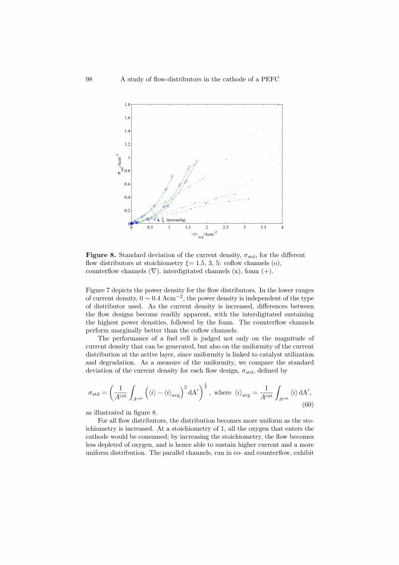
98 A study of flow-distributors in the cathode of a PEFC
0 0.5 1 1.5 2 2.5 3 3.5 40
0.2
0.4
0.6
0.8
1
1.2
1.4
1.6
1.8
<i>avg
/Acm-2
σ std/A
cm-2
ξ increasing
Figure 8. Standard deviation of the current density, σstd, for the differentflow distributors at stoichiometry ξ= 1.5, 3, 5: coflow channels (o),counterflow channels (∇), interdigitated channels (x), foam (+).
Figure 7 depicts the power density for the flow distributors. In the lower rangesof current density, 0 ∼ 0.4 Acm−2, the power density is independent of the typeof distributor used. As the current density is increased, differences betweenthe flow designs become readily apparent, with the interdigitated sustainingthe highest power densities, followed by the foam. The counterflow channelsperform marginally better than the coflow channels.
The performance of a fuel cell is judged not only on the magnitude ofcurrent density that can be generated, but also on the uniformity of the currentdistribution at the active layer, since uniformity is linked to catalyst utilizationand degradation. As a measure of the uniformity, we compare the standarddeviation of the current density for each flow design, σstd, defined by
σstd =
µ1
Acat
ZAcat
³hii− hiiavg
´2dA0
¶ 12
, where hiiavg =1
Acat
ZAcat
hiidA0,(60)
as illustrated in figure 8.For all flow distributors, the distribution becomes more uniform as the sto-
ichiometry is increased. At a stoichiometry of 1, all the oxygen that enters thecathode would be consumed; by increasing the stoichiometry, the flow becomesless depleted of oxygen, and is hence able to sustain higher current and a moreuniform distribution. The parallel channels, run in co- and counterflow, exhibit

E. Birgersson and M. Vynnycky 99
the highest deviations at current densities above ∼ 0.4 Acm−2, with the coflowbeing the less uniform of the two. At current densities below 1.5-2 Acm−2,depending on stoichiometry, greatest uniformity is obtained for the interdigi-tated design, but the extent of the non-uniformity increases with the current;ultimately, the foam design gives the greatest uniformity. These findings arealso reflected in figures A1-A4, where the local current density for differentcell potentials is given. All distributors exhibit a more non-uniform currentdensity as the overpotential is increased, i.e. as the cell voltage decreases.For coflow (see figure A1), the areas under the flow channels can sustain localhigher current densities than those under the "rib" of the bipolar plate, wheremass transfer becomes increasingly limiting with increasing overpotential. Thecathode operated in counterflow behaves similarly (figure A2), but delivers asomewhat higher overall performance, as the counterflow arrangement allowsfor exiting air with a lower oxygen concentration in one channel to be balancedby incoming fresh air in the two adjacent channels. For the foam (figure A3),the local current density is a function of the streamwise coordinate only, al-though there are minor inlet and exit effects, which become somewhat morepronounced at higher current densities. This simplification is attributable tothe inherent characteristic of the foam to cover the surface of the porous back-ing, in contrast to grooved channels in a bipolar plate comprising alternatingregions of channels and ribs. Finally, the interdigitated arrangement (figureA4) displays an increasingly spanwise behaviour for the local current densityat higher overpotentials. The overall flow increases for a given stoichiometryat higher current densities, leading to increased forced convective flow in theporous backing, whence the local current density becomes more even in thespanwise direction.
Keeping the pressure drop, ∆p¡= pin − pout
¢, at a minimum is of interest
in terms of reducing operating costs for the fuel cell, whence the optimal flowdistributor should be able to sustain high even current densities, whilst keepingthe pressure drop to a minimum. The foam, as shown in figure 9, requires thehighest pressure drop to drive the flow; this can be attributed to the rather lowpermeability chosen for the foam in this study. An increase in permeability to10−8 m2 would lead to a reduction of the pressure drop by approximately 2orders of magnitude, as can be estimated from Darcy’s law. The pressure dropfor the interdigitated distributor is higher than for the coflow and counterflow,which is to be expected since the flow is being forcibly driven through the porousbacking, in this study with a permeability of 10−12 m2. The lowest pressuredrops are obtained with the parallel channels, with no discernible difference inthe magnitude of the pressure drop between the two.

100 A study of flow-distributors in the cathode of a PEFC
0 0.5 1 1.5 2 2.5 3 3.5 4100
101
102
103
104
<i>avg
/Acm-2
∆ p/N
m-2
ξ increasing
Figure 9. Pressure drop, ∆p, for the different flow distributors atstoichiometry ξ = 1.5, 3, 5: coflow channels (o), counterflow channels (∇),interdigitated channels (x), foam (+).
0 0.5 1 1.5 2 2.5 3 3.5 40
5
10
15
20
25
30
<i>avg
/Acm-2
Uin
/ms-1
ξ increasing
Figure 10. Obtained inlet velocity, U in, for the different flow distributors atstoichiometry ξ = 1.5, 3, 5: coflow channels (o), counterflow channels (∇),interdigitated channels (x), foam (+).
E. Birgersson and M. Vynnycky 101
Since we do not specify the inlet velocity, but rather iterate on it to obtaina given stoichiometry for a specified cell potential, it is of interest to see howthe inlet velocity changes with current density and stoichiometry; this is shownin figure 10. The inlet velocity is almost proportional to the average currentdensity, and only starts to deviate from linear when the density at the inletchanges due to the pressure drop obtained. The reason why the inlet velocitiesfor the interdigitated channels are higher is because the inlet area is half aslarge as for the other flow distributors.
5. Conclusions
A study of different flow distributors, based on a gas-phase model for mass,momentum and species transport in the cathode of a PEM fuel cell, has beenconsidered. Special attention was given to the treatment of the active layer, forwhich an agglomerate model developed previously [9] was used. The numericalcode used was verified with an analytical solution also developed previously [3].The novel features of this study are: 1) a direct quantitative comparison ofthe performance of different flow distributors; 2) the use of a new Tafel lawwhich agrees well with experimental observations for a small fuel cell [13]. Thecomplete validation of the gas-phase model considered here would require moredetailed information about the local current density distribution; in future, thiswill be obtainable via experiments with a segmented cell.
The aim of the study was to compare the performance of different flow dis-tributors for a given cell at a given potential, in terms of four different quanti-ties: the obtained average current density, power density, standard deviation ofthe current density distribution and pressure drop. The results show that theinterdigitated flow distributor can sustain the highest current densities, but ata higher pressure drop than the counterflow and coflow channels. Furthermore,to function properly, the interdigitated channels would have to be in contactwith the porous backing in such a way that channeling effects are kept at aminimum; given the high velocities required, even the slightest gap might leadto most of the flow going through the gap and not through the porous backing,with a resulting loss of power density. A foam distributor is able to give thelowest standard deviation for the current at high current densities, but careshould be taken as to its permeability to avoid an unreasonably high pressuredrop.
The present work was limited to gas-phase flow and isothermal conditions.Future work will seek to incorporate both the possible production of liquidwater at the catalytic layer and non-isothermal effects.
Acknowledgements
Financial support from the Swedish Foundation for Strategic Environmen-tal Research, MISTRA, and from the Swedish National Energy Administrationis gratefully acknowledged. The work was done within the framework of theJungner Center.
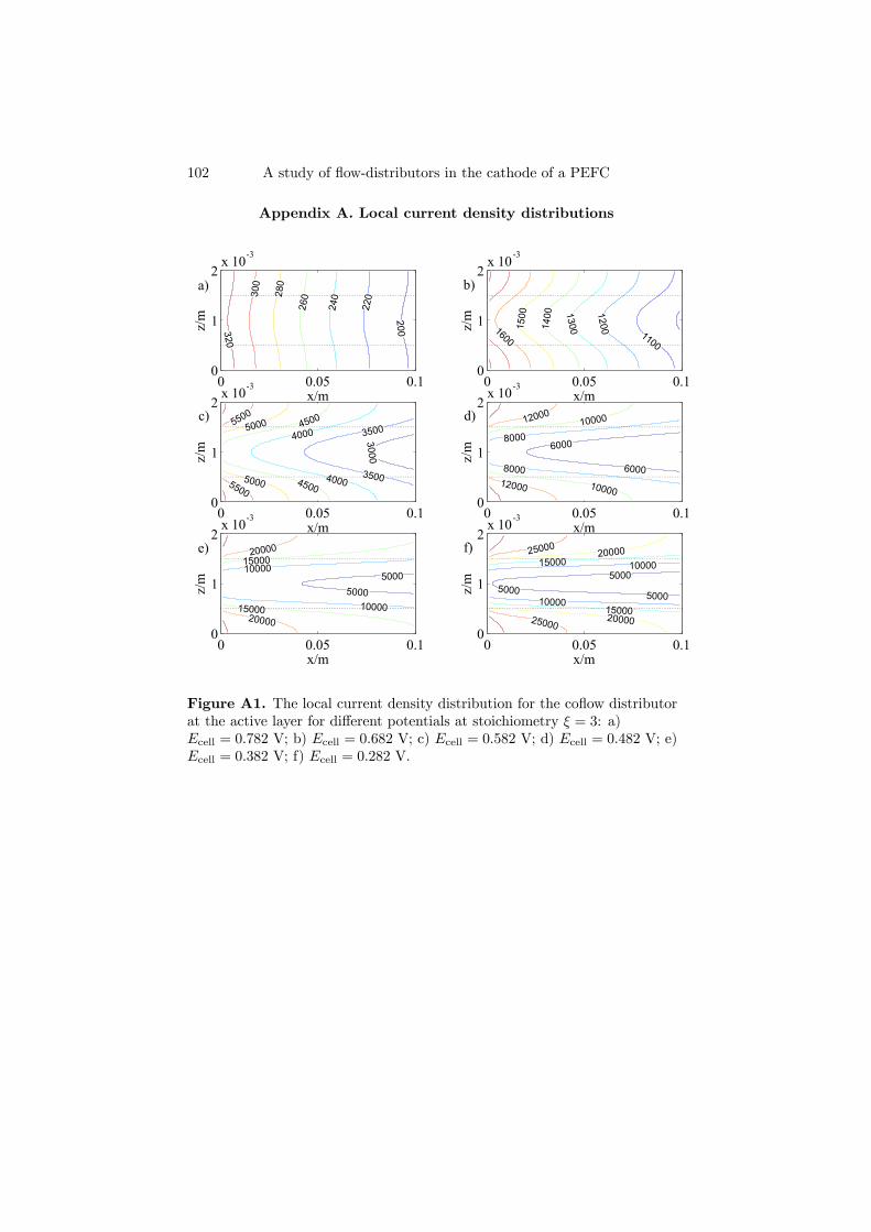
102 A study of flow-distributors in the cathode of a PEFC
Appendix A. Local current density distributions
0 0.05 0.10
1
2x 10⁻³
x/m
z/m 200
220
240
26028
0
300
320
0 0.05 0.10
1
2x 10⁻³
x/m
z/m
1100
1200
13001400
1500
1600
0 0.05 0.10
1
2x 10⁻³
x/m
z/m
3000
3500
3500
4000
4000
4500
4500
5000
5000
5500
5500
0 0.05 0.10
1
2x 10⁻³
x/m
z/m 6000
6000
8000
8000
10000
10000
12000
12000
0 0.05 0.10
1
2x 10⁻³
x/m
z/m 5000
5000
10000
10000
15000
15000
20000
20000
0 0.05 0.10
1
2x 10⁻³
x/m
z/m 5000
5000 5000
10000
10000
15000
15000
20000
20000
25000
25000
a) b)
c) d)
e) f)
Figure A1. The local current density distribution for the coflow distributorat the active layer for different potentials at stoichiometry ξ = 3: a)Ecell = 0.782 V; b) Ecell = 0.682 V; c) Ecell = 0.582 V; d) Ecell = 0.482 V; e)Ecell = 0.382 V; f) Ecell = 0.282 V.

E. Birgersson and M. Vynnycky 103
0 0.05 0.10
1
2x 10⁻³
x/m
z/m
160
160
180
180
200
200220
220
240
240
260
260
280
280
0 0.05 0.10
1
2x 10⁻³
x/m
z/m 1200
1200
1300
1300
1400
1400
1500
1500
1600
0 0.05 0.10
1
2x 10⁻³
x/m
z/m
3500
35003500
35004000
4000
4500
4500
5000
5000
0 0.05 0.10
1
2x 10⁻³
x/mz/
m
6000600060006000
80008000
8000800010000
10000
12000
12000
0 0.05 0.10
1
2x 10⁻³
x/m
z/m 5000
5000
10000
1000015000
15000
20000
20000
0 0.05 0.10
1
2x 10⁻³
x/m
z/m 5000
50005000
10000
10000
15000
1500020000
20000
25000
25000
a) b)
d) c)
e) f)
Figure A2. The local current density distribution for the counterflowdistributor at the active layer for different potentials at stoichiometry ξ = 3:a) Ecell = 0.782 V; b) Ecell = 0.682 V; c) Ecell = 0.582 V; d) Ecell = 0.482 V;e) Ecell = 0.382 V; f) Ecell = 0.282 V.

104 A study of flow-distributors in the cathode of a PEFC
0 0.05 0.10
1
2x 10⁻³
x/m
z/m
200
22024026
0
280
300320
0 0.05 0.10
1
2x 10⁻³
x/m
z/m 12
00
1300
1400
1500
16001700
18001900
0 0.05 0.10
1
2x 10⁻³
x/m
z/m
4000
45005000
5500
6000
6500
0 0.05 0.10
1
2x 10⁻³
x/m
z/m
100001200
0
1400
0
1600
0
18000
0 0.05 0.10
1
2x 10⁻³
x/m
z/m
1800
0
20000
220002400
0
2600
0
2800
0
30000
0 0.05 0.10
1
2x 10⁻³
x/m
z/m 25
000
3000
0
3500
0
a) b)
d) c)
e) f)
Figure A3. The local current density distribution for the foam distributor atthe active layer for different potentials at stoichiometry ξ = 3: a)Ecell = 0.782 V; b) Ecell = 0.682 V; c) Ecell = 0.582 V; d) Ecell = 0.482 V; e)Ecell = 0.382 V; f) Ecell = 0.282 V.

E. Birgersson and M. Vynnycky 105
0 0.05 0.10
1
2x 10⁻³
x/m
z/m
180
200
220
240260
280
300320
0 0.05 0.10
1
2x 10⁻³
x/m
z/m 1000
12001400
1600
0 0.05 0.10
1
2x 10⁻³
x/m
z/m
4000450045005000
5000
5500
5500
60006500
0 0.05 0.10
1
2x 10⁻³
x/m
z/m
120001400016000
18000
2000020000
a) b)
d) c)
Figure A4. The local current density distribution for the interdigitated flowdistributor at the active layer for different potentials at stoichiometry ξ = 3:a) Ecell = 0.782 V; b) Ecell = 0.682 V; c) Ecell = 0.582 V; d) Ecell = 0.482 V.
106 A study of flow-distributors in the cathode of a PEFC
List of symbolsA Area, m2
A Integration constant for asymptotic solutionAi0 Volumetric exchange current density, A m−3
B Transformation tensorB Integration constant for asymptotic solutionc Molar concentration, mol m−3
D Diffusion tensor, m2s−1eDij Diffusion coefficients for molar diffusive fluxrelative to a molar-averaged velocity, m2s−1
Dij Diffusion coefficients for mass diffusive fluxrelative to a mass-averaged velocity, m2s−1
Dij Binary Maxwell-Stefan diffusion coefficients, m2s−1
D Effective oxygen permeability in the agglomerates, mol m−1s−1
∆p Pressure drop, Nm−2
ex, ey, ez Coordinate vectorsE Potential, VF Faraday’s constant, As mol−1
F Nucleus effectiveness factor for the agglomerate modelh Height, mh Relative humidityi Current density, A m−2
hivi Volume current density, A m−3
I Dimensionless current densityK Permeability tensor, m2
L Length, mM Mean molecular mass, kg mol−1
M Dimensionless mean molecular massMi Molecular mass of species i, kg mol−1
Mi Dimensionless molecular mass of species in Number of electrons consumed in the ORR per oxygen moleculen Unit vector in the normal directionni Mass flux of species i, kg m−2s−1
p Pressure, Nm−2
P Power density, Wm−2
r Radius of agglomerate nucleus, mR Gas constant, J mol−1 K−1
Re Reynolds numberS Denominator for transformation of diffusion coefficients, m2s−1
t Unit vector in the tangential directionT Temperature, Kv Velocity, ms−1
V Volume of the representative elementary volume, m3
w Width, mwi Mass fraction of species i
E. Birgersson and M. Vynnycky 107
W Transformation tensorxi Molar fraction of species iX, Y Dimensionless coordinatesX Transformation tensorGreekα Coefficient for water transport
in the membraneαr Cathodic transfer coefficient for the ORRγ Porosityδij Kronecker delta∆ = 1/(Reσ2) Dimensionless parameterζ i Dimensionless fraction of species iη Overpotential, Vκ Permeability, m2
µ Dynamic viscosity, kg m−1 s−1
ξ Stoichiometryρ Density, kg m−3
σ = hf/L Dimensionless numberσstd Standard deviation for current density, Am−2
Υ Parameter for current density expressionφ General tensorΦ = (2 + 4α)MH2O −MO2 Dimensionless numberΩ = Λ/σ Dimensionless numberSubscripts0 Equilibrium, Referencea Active layercell Cellp Porous backingpol Polymer electrolyte in the active layerf Flow channelH2O WaterO2 OxygenN2 Nitrogenavg AverageSuperscriptscat Catalytic regiong Gasin Inletout Outletref Referencevap VaporisationMiscellaneous symbolsh i Superficial averageh i(g) Intrinsic average[ ] Scale

Bibliography
[1] C. K. Dyer, J. Power Sources, Proceedings of the Seventh Grove Fuel Cell Symposium,106, 31 (2002).
[2] J. M. Moore, J. B. Lakeman and G. O. Mepsted, J. Power Sources, Proceedings of theSeventh Grove Fuel Cell Symposium, 106, 16 (2002).
[3] M. Vynnycky and E. Birgersson, SIAM (Soc. Ind. Appl. Math ), 63, 1392 (2003).[4] S. Dutta, S. Shimpalee and J. W. van Zee, J. Appl. Electrochem., 30, 135 (2000).[5] S. Dutta, S. Shimpalee and J. W. van Zee, Int. J. Heat and Mass Transfer, 44, 2029
(2001).[6] S. Shimpalee and S. Dutta, Numerical Heat Transfer, 38, Part A, 111 (2000).[7] P. Costamagna, Chem. Eng. Science, 56, 323 (2001).[8] T. Berning, D. M. Lu and N. Djilali, J. Power Sources, 106, 284 (2002).[9] F. Jaouen, G. Lindbergh and G. Sundholm, J. Electrochem. Soc., 149, A437 (2002).[10] CFX-4.4, http://www.cfx.aeat.com.[11] R. Taylor and R. Krishna, Multicomponent Mass Transfer, John Wiley & Sons, USA
(1993).[12] J. R. Welty, C. E. Wicks and R. E. Wilson, Fundamentals of Momentum, Heat, and
Mass Transfer, 3rd edition, John Wiley & Sons, USA (1984).[13] J. Ihonen, F. Jaouen, G. Lindbergh, A. Lundblad and G. Sundholm, J. Elec-
trochem. Soc., 149, A448 (2002).[14] M. J. Moran and H. N. Shapiro, Fundamentals of Engineering Thermodynamics, 2nd
edition, John Wiley & Sons, USA (1993).[15] J.S.Yi and T. Van Nguyen, J. Electrochem. Soc., 146, 1 (1999).[16] A. Kazim, H.T. Liu and P. Forges, J. Appl. Electrochem., 29, 1409 (1999) .
108

Paper 3


Analysis of a Two-Phase Non-Isothermal Modelfor a Polymer Electrolyte Fuel Cell
E. Birgerssona, M. Noponenb and M. Vynnyckya
aDepartment of Mechanics, FaxénLaboratoriet, The Royal Institute of Technology,SE-100 44, Stockholm, SwedenbEnergy production, VTT Process, Biologinkuja 5, Espoo, FIN-020 44 VTT, Finland
Abstract. A non-isothermal, two-phase model for a polymer electrolyte fuelcell is presented, analysed and solved numerically under three different thermal, andtwo hydrodynamic, modelling assumptions; the consequences of these are then dis-cussed in terms of thermal and water management and cell performance. The studyis motivated by recent experimental results that suggest the presence of previouslyunreported, and thus unmodelled, thermal contact resistances between the compo-nents of a PEFC [1], and the discrepancy in the value for the capillary pressure that isused by different authors when modelling the two-phase flow in a PEFC. In the threecases that deal with varying thermal conditions (assuming: effective heat conductiv-ities for all components; isothermal flow; interfacial and bulk conductivities, betweenand for components, respectively), liquid saturations of around 10% are obtained atthe cathode active layer for 1000 mAcm−2 and a cell voltage of 0.6 V, in contrastto almost 50 % (locally up to 100%) for the fourth, where the capillary pressure istaken to be three orders of magnitude lower than in the first three. At this currentdensity and voltage, temperature differences across the cell of around 5oC are pre-dicted. The benefits of the scaling analysis conducted here, to predict correctly, priorto numerical computations, important characteristic cell performance quantities suchas current density and temperature drop, are also highlighted.
1. Introduction
The polymer electrolyte fuel cell (PEFC) is a promising alternative to tra-ditional power sources for a wide range of potential, automotive and stationaryapplications. Despite the many advantages of PEFCs, such as high efficiencyand low emissions, substantial technological improvements are still one of themain prerequisites for the PEFC to be able to contend with existing powersources. Such improvements will come through an understanding of the cou-pling of kinetics and transport phenomena at the heart of a PEFC system, aunit cell comprising several distinct components: the membrane electrode as-sembly (MEA), gas diffusion backings and bipolar plates. The MEA consistsof an electrolyte, i.e. a proton conducting membrane, sandwiched between twoelectrodes. Adjacent to each electrode is a porous backing, also known as thegas diffusion layer, and a bipolar plate, as illustrated in Figure 1. On the anodeside, hydrogen is oxidized into electrons, which can drive a load in an external
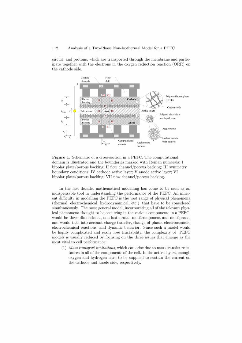
112 Analysis of a Two-Phase Non-Isothermal Model for a PEFC
circuit, and protons, which are transported through the membrane and partic-ipate together with the electrons in the oxygen reduction reaction (ORR) onthe cathode side.
+
-
e- Membrane Active layers
Agglomeratenucleus
Porousbacking
Porousbacking
Flowfield
Anode
Cathode
Polymer electrolyteand liquid water
Carbon particlewith catalyst
Agglomerate
Polytetrafluorethylene(PTFE)
Carbon cloth
Coolingchannels
Computationaldomain
I II
IV
VI
III
VII
V
III
III
III
III
III
hc
hMEA
ha
wws
ey
exez
y
x
Figure 1. Schematic of a cross-section in a PEFC. The computationaldomain is illustrated and the boundaries marked with Roman numerals: Ibipolar plate/porous backing; II flow channel/porous backing; III symmetryboundary conditions; IV cathode active layer; V anode active layer; VIbipolar plate/porous backing; VII flow channel/porous backing.
In the last decade, mathematical modelling has come to be seen as anindispensable tool in understanding the performance of the PEFC. An inher-ent difficulty in modelling the PEFC is the vast range of physical phenomena(thermal, electrochemical, hydrodynamical, etc.) that have to be consideredsimultaneously. The most general model, incorporating all of the relevant phys-ical phenomena thought to be occurring in the various components in a PEFC,would be three-dimensional, non-isothermal, multicomponent and multiphase,and would take into account charge transfer, change of phase, electroosmosis,electrochemical reactions, and dynamic behavior. Since such a model wouldbe highly complicated and easily lose tractability, the complexity of PEFCmodels is usually reduced by focusing on the three issues that emerge as themost vital to cell performance:
(1) Mass transport limitations, which can arise due to mass transfer resis-tances in all of the components of the cell. In the active layers, enoughoxygen and hydrogen have to be supplied to sustain the current onthe cathode and anode side, respectively.

E. Birgersson, M. Noponen and M. Vynnycky 113
(2) Thermal management, to ensure that the heat generated throughoutthe cell, in particular at the active layer of the cathode, is removedby adequate cooling of the cell.
(3) Water management, to prevent flooding of the various components inthe fuel cell whilst ensuring that the membrane remains sufficientlyhydrated to keep the ohmic losses at a minimum.
The most recent models [2—11] address two or more of these issues. He,Yi and Nguyen [2], Natarajan and Nguyen [3], Wang, Wakayama and Okada[4], You and Liu [5], Wang, Wang and Chen [6] focus on the mass transportlimitations (1) and water management (2) in a two-dimensional cathode andassume isothermal conditions. All three issues (1-3) are considered for the wholecell by Djilali and Lu [7], Janssen [8] and Wöhr et al. [9] for a one-dimensionalgeometry and by Berning and Djilali [10] and Mazumder and Cole [11] for athree-dimensional geometry.
With respect to thermal management alone, none of the above addressthe contact resistances that can occur between the various components of thecell. This observation is based on recent experimental findings Ihonen et al. [1],who observed that the thermal conductivity is a function of clamping pressure,and concluded that the interfacial conductivity is much lower than the bulkconductivity for heat transfer. Vie [12] measured the thermal conductivity andfound it to be approximately 0.2 W m−1K−1 for a E-TEK gas diffusion layer,whereas Ihonen et al. [1] arrived at values between 0.2 and 0.5 W m−1K−1 fordifferent materials.
With respect to the water management, on the other hand, there appearto be wide discrepancies in the value of the capillary pressure that is usedby different authors for the modelling of the two-phase flow in the porousbackings [3, 6]; how this is modelled will, in turn, have implications on thethermal management.
The main goals of this paper are to ascertain by means of a mathematicalmodel the impact of capillary pressure and interfacial conductivity, as wellas low bulk conductivities, on thermal and water management in a PEFC.First, the model, consisting of two-phase, steady-state, mass, momentum, heat,charge and species conservation equations in the porous backing of the cathode,coupled with heat transfer and conservation of charge for the membrane andanode, is introduced. The model equations are nondimensionalised, and a scaleanalysis is carried out, so as to determine the relative importance of competingtransport phenomena prior to numerical computation, as well as to provide ananalytical interpretation of the computed results. These are obtained underthree different thermal, and two hydrodynamic modelling assumptions: (a)without and with (c) thermal contact resistances; (b) isothermal conditions;(d) as in (a) but with a capillary pressure taken to be three orders of magnitudelower.

114 Analysis of a Two-Phase Non-Isothermal Model for a PEFC
2. Mathematical formulation
A cross section at a given location in the streamwise direction of the PEFCis considered in this study, as illustrated in Figure 1. This entails omitting thestreamwise direction (ez), but retaining the spanwise (ex) and normal (ey)directions. The domain under consideration consists of the porous backings ofthe anode and cathode, and the membrane, with origin in the middle of themembrane, as shown in Figure 1. The domain’s boundaries and interfaces aredenoted with roman numerals.
Since the cathode is the limiting side of the PEFC, we will consider all threeof the aforementioned phenomena (1-3) there. In the anode and membrane,only the thermal management (2) will be taken into account. Neglecting masstransfer limitations (1) and water management (3) in these two components is areasonable approximation, provided that the hydrogen feed is well humidified,the stoichiometry is sufficiently high and there is no poisoning of the catalyst atthe anode. We will later show, through scale analysis, that the convective heattransfer is negligible compared to the conductive heat transfer in the porousbackings of the cathode and anode; therefore, for the sake of brevity, the heatconvection will be excluded from the anode side from the outset. Transportphenomena in the actual flow channels and ribs are not resolved, but are treatedwith appropriate boundary conditions for the domain of interest.
The model accounts for the following transport phenomena:
• Heat transfer: Conduction is considered in the porous backings ofthe cathode and anode, as well as in the membrane; a scale analysiswill show convective heat transfer to be negligible. In addition, ohmicheating stemming from the resistance to charge transfer is accountedfor in the whole domain. The heat generated at the active layer ofthe cathode from the oxygen reduction reaction is accounted for interms of entropy change and irreversibilities. Another heat source isthe latent heat of vaporization of the liquid water originating fromthe membrane water flux and ORR at the cathode.
• Charge transfer: Conservation of charge is solved for throughoutthe domain.
• Mass, momentum and species transfer: Conservation of two-phase mass, species and momentum is considered in the cathode.
The main model assumptions/approximations are:
• Thermal equilibrium: Local thermal equilibrium is assumed be-tween the phases in the porous backings of the anode and cathode, aswell as in the membrane.
• 2D cross section: A general PEFC model would have to be three-dimensional. In order to reduce the fuel cell to a two-dimensionalgeometry which describes a cross section, the model is limited tocells, in which the changes in the streamwise direction in the flowdistributors are small. This applies to cells operated at a high oxygenand hydrogen stoichiometry. The model derived here was validated

E. Birgersson, M. Noponen and M. Vynnycky 115
by Noponen et al. [13] for case a (see below) with experimental datafrom a segmented cell with a net-type flow field, in which the currentdensity distribution could be considered constant in the streamwisedirection of the flow.
• Membrane: The water flux in a membrane is modelled with a con-stant water drag coefficient. This simplification is necessary, since noreliable data for the water transport in the type of membrane (GorePrimea 5510) that we consider here could be found from availableliterature.
• Anode: Only heat and charge transfer is considered in the anode,and thus it is assumed that the anode is running at such conditionsthat it can sustain the currents obtained, i.e. at sufficiently high hy-drogen stoichiometry, humidification and little or no carbon monoxidepoisoning of the catalyst. Since we do not solve for the mass transfer,we cannot model any heat of vaporization at the anode. The over-potential at the active layer is assumed negligible compared to theactivation overpotential at the cathode.
• Flow channels: It is assumed here that the heat transfer to thechannels from the porous backing (boundaries II, VII) is negligiblecompared to the heat transfer by conduction to the current collectors.At the flow channel of the cathode (boundary VII), we assume that theliquid water removal is sufficiently fast, so that the liquid saturationcan be set to zero there.
• Cathode active layer: The active layer on the cathode side is con-sidered as an interface and is not resolved spatially. The active layeris, however, very thin in comparison with the porous backing, so thatthe macroscopic properties such as oxygen concentration will be moreor less constant across it, see [14]. Furthermore, it is assumed that thewater from the ORR and membrane is in liquid form when it entersthe porous backing of the cathode side. An expression for the currentdensity was obtained from parameter adaption to experimental datafrom a segmented cell [13].
• Electric contact resistances: At interfaces I,V and VI, the electriccontact resistance is accounted for in the charge transfer. At thecathode active layer, the electric contact resistance is taken to benegligible compared to the activation overpotential, since the cathodeactivation overpotential at 1000 mAcm−2 is around 10−1 V, comparedto a voltage drop of ∼10−3 V for the contact resistance.
• Two-phase flow: The amount of water in the porous backing ofthe cathode is determined by properties such as the mobilities of theliquid and gas phases and the capillary pressure. No experimentaldata is currently available in the literature for these parameters. Inaddition, the solubilities of nitrogen and oxygen are sufficiently lowto allow us to treat the liquid phase as water only. The capillarypressure and relative mobilities from [6] will be applied to cases a-c,
116 Analysis of a Two-Phase Non-Isothermal Model for a PEFC
outlined below. An alternative capillary pressure [3] will be examinedin case d.
Within this framework, and as already motivated in the Introduction, thispaper will compare the consequences of four particular additional modellingassumptions:
a) an effective heat conductivity is considered for the porous backings ofthe anode and cathode;
b) isothermal conditions are assumed, where the temperature of the cellis kept at 60 oC;
c) bulk and interface contact conductivities are treated.
The fourth concerns the capillary pressure:
d) an expression employed by Natarajan and Nguyen [3] is used andan effective heat conductivity for heat transfer is assumed. This [3]differs by three orders of magnitude from the term introduced byWang, Wang and Chen [6], and, as we shall see later, the formerwill give rise to a significant increase in liquid water content in thecathode, compared to the latter.
3. Governing equations
In this paper, the superscripts (g) and (l) denote properties associated withthe gas and liquid phase, respectively, and (c) is for any quantity associated withthe capillary pressure. All properties are intrinsic, except the velocities, massfluxes and current density, which are superficial. The two-phase formulationis based on a separate flow model approach [2, 3, 7—10], where we treat theliquid and gas phases separately, in contrast to the multiphase mixture modelapproach [5, 6,11].
3.1. Cathode. In the porous backing of the cathode, we solve for theconservation of mass and momentum of the liquid and gas phase. These areexpressed by
∇ ·³ρ(g)v(g)
´= − ·
mH2O, (1)
∇ ·³ρ(l)v(l)
´=
·mH2O, (2)
∇p(g) = − µ(g)
κκ(g)rel
v(g) + ρ(g)g, (3)
v(l) =κ(l)relµ
(g)
κ(g)relµ
(l)v(g) +
κκ(l)rel
µ(l)∇p(c) + κκ
(l)rel
µ(l)(ρ(l) − ρ(g))g, (4)
where ρ(g,l) denote the phase densities, v(g,l) = (u(g,l), v(g,l)) are the phasevelocities (in the x and y directions, see Fig. 1),
·mH2Ois the interface mass
transfer of water between the gas and liquid phase, p(g,l) are the phase pressures,

E. Birgersson, M. Noponen and M. Vynnycky 117
µ(g,l) are the phase dynamic viscosities, κ is the permeability, κ(g,l)rel are therelative permeabilities of the phases.
The amount of liquid water is given by the liquid saturation, s, defined as
s =V(l)
V(l) + V(g) , (5)
where V(k) is the volume occupied by phase k in a representative elementaryvolume.
The conservation of charge together with Ohm´s law yields
∇2φs = 0, (6)
where φs is the electric potential of the solid phase of the porous backing. Inaddition, we solve for a ternary mixture of water, nitrogen and oxygen in thegas phase, given by
∇ ·"n(g)O2
n(g)H2O
#+
·0
·mH2O
¸= 0, (7)
with the species mass fluxes, n(g)O2and n(g)H2O, given by"
n(g)O2
n(g)H2O
#= ρ(g)v(g)
"w(g)O2
w(g)H2O
#− ρ(g)γ
32 (1− s)D(g)
"∇w(g)O2
∇w(g)H2O
#, (8)
where D(g) is a multicomponent mass diffusion tensor,·mH2Ois the interface
mass transfer, γ is the porosity and w(g)H2O
and w(g)O2are the mass fractions of
water and oxygen in the gas phase, respectively. The species mass fluxes in thegas phase are written in a compact form, to be read as two equations, one foroxygen and the other for water, which are coupled through the diffusion tensorD(g).
The heat transfer is given by³c(g)p,O2
n(g)O2+ c
(g)p,H2O
n(g)H2O
+ c(l)p,H2O
ρ(l)v(l)´·∇T
= ∇ · (kc∇T ) +Hvap·mH2O + σc (∇φs)
2; (9)
here T is the temperature, kc is the effective thermal conductivity (case a and d)or a bulk conductivity (case c), c(k)p,i is the specific heat capacity of species i andphase k, σc is the electric conductivity andHvap is the enthalpy of vaporization.The two last terms on the RHS of Eq. A.10 account for the heat of vaporizationand ohmic heating, respectively.
3.2. Anode. On the anode side, we solve for conservation of heat, to-gether with conservation of charge and Ohm´s law:
∇ · (ka∇T ) + σa (∇φs)2= 0,
∇2φs = 0, (10)
118 Analysis of a Two-Phase Non-Isothermal Model for a PEFC
The mass transfer of hydrogen and water in the binary mixture on the anodeside is assumed to be sufficient to sustain the currents obtained. Essentially,this means that the anode side is operated under such conditions that it doesnot limit the performance of the cell.
3.3. Membrane. In the membrane, we solve for conservation of heat andcharge together with Ohm’s law, given by
∇ ·¡keffm ∇T
¢+ σm (∇φm)
2= 0, (11)
∇2φm = 0, (12)
where φm is the potential in the ionic phase. The effective water flux throughthe membrane is modelled with a drag coefficient, α; this limits the model toheat transfer predictions, and thus effects such as dehydration of the membraneand electrodes cannot be studied. If these effects are of interest, then a moredetailed membrane and anode model should be used, see e.g. [15—18]. Aneffective conductivity of the membrane is considered for all the cases.
4. Boundary conditions
4.1. Anode bipolar plate/porous backing (I). The boundary con-dition for the potential includes the contact resistance, rcont, and is writtenas
−σa∂φs∂y
=φa,0 − φsrcont
, (13)
where we set φa,0 = 0.The boundary condition used for temperature in the case of effective heat
conductivity (a, d) is given by continuity of temperature as
T = T cool, (14)
whereas for the case of thermal interface conductivity (c), we use a similarexpression as for the potential, Eq. 13,
−kbulka
∂T
∂y= −Kcont
¡T − T cool
¢, (15)
where Kcont is the interfacial heat conductivity. This boundary condition isalso known as Newton’s law of cooling.
4.2. Anode flow channel/porous backing (II). It is assumed that theheat transfer into the flow channel is small compared to the heat flux to therib; thus, we set
∂T
∂y=
∂φs∂y
= 0. (16)
E. Birgersson, M. Noponen and M. Vynnycky 119
4.3. Symmetry boundary conditions (III). At the right and left sidesof the domain of interest, we specify symmetry boundary conditions
u(g) = n(g)O2· ex = n(g)H2O · ex =
∂φs∂x
=∂T
∂x=
∂s
∂x= 0, (cathode) (17)
∂φm∂x
=∂T
∂x= 0, (membrane) (18)
∂φs∂x
=∂T
∂x= 0, (anode) (19)
4.4. Cathode active layer (IV). The active layer is reduced to an in-terface between the membrane and the porous backing, with the gas and liquidmass fluxes there given by
ρ(g)v(g)¯IV+
= − icMO2
4F, (20)
ρ(l)v(l)¯IV+
=ic4F
(2 + 4α)MH2O, (21)
where ic is the current density. The componential fluxes in the gas phase are"n(g)O2
n(g)H2O
#IV+
· ey = −ic4F
µMO2
0
¶. (22)
For the case of an effective heat conductivity (a, d), we have continuity oftemperature, so that
T |IV− = T |IV+ , (23)
and the heat fluxes on either side of the interface are related byµ³c(g)p,O2
n(g)O2+ c
(l)p,H2O
ρ(l)v(l)´· ey(T − T cool)− keffc
∂T
∂y
¶IV+
= ic
Ã−T |IV− ∆SPt,c
4F− ηc
!+
µ−keffm
∂T
∂y
¶IV−
, (24)
where ηc (≤ 0) is the cathode overpotential. For the case of the thermalinterface conductivity (c), the appropriate conditions areµ−keffm
∂T
∂y
¶IV−
= −Ã−T |IV− ∆SPt,c
4F− ηc
!ic +Kcont
³T |IV− − T |IV+
´,
(25)µ³c(g)p,O2
n(g)O2+ c
(l)p,H2O
ρ(l)v(l)´· ey(T − T cool)− kbulkc
∂T
∂y
¶IV+
= Kcont³T |IV− − T |IV+
´. (26)
The interface conditions for the current production are
−σm∂φm∂y
¯IV−
= ic, − σc∂φs∂y
¯IV+
= ic. (27)

120 Analysis of a Two-Phase Non-Isothermal Model for a PEFC
4.5. Anode active layer (V). At the anode, the activation is assumednegligible compared to the contact resistance, so we take
−σa∂φs∂y
¯V−
=φs − φmrcont
, − σm∂φm∂y
¯V+
=φs − φmrcont
. (28)
The temperature and heat flux are continuous for the case of an effectiveheat conductivity (a), so that
T |V− = T |V+ , (29)
−keffa∂T
∂y
¯V−
= −keffm∂T
∂y
¯V+
. (30)
For the case of the interface contact resistance (c, d), only the heat flux isassumed continuous:
−keffm∂T
∂y
¯V+
= −Kcont³T |V+ − T |V−
´, (31)
−kbulka
∂T
∂y
¯V−
= −Kcont³T |V+ − T |V−
´. (32)
For the anode, the entropy production ∆SPt,a ∼10−1 J mol−1 K−1 [19] is solow that it can be neglected compared to the entropy production ∆SPt,c ∼300J mol−1 K−1 [19] at the cathode . It should be noted that these values arebased on the assumption that only the gas phase and platinum are in contact,and therefore the values are likely to be somewhat different for a PEFC, whereplatinum is also in contact with the ion and electric conductors.
4.6. Cathode bipolar plate/porous backing (VI). For the potential,we once again employ a contact resistance boundary condition:
−σc∂φs∂y
=φs −Ecell
rcont. (33)
In addition, there is no normal flow and no normal mass flux in all phases;these are then expressed as
v(g) =∂w
(g)O2
∂y=
∂w(g)H2O
∂y=
∂s
∂y= 0.
For temperature, in the case of the effective heat conductivity (a, d), we have
T = T cool, (34)
whereas for the case of the interface heat conductivity (c),
−kbulkc
∂T
∂y= Kcont
¡T − T cool
¢. (35)
E. Birgersson, M. Noponen and M. Vynnycky 121
4.7. Cathode flow channel/porous backing (VII). The mass frac-tions of oxygen and water, the gas pressure, liquid saturation and the electricand heat fluxes are prescribed as follows:
w(g)O2= w
(g)O2,0
, w(g)H2O
= w(g)H2O,0
, p(g) = p(g)0 , s = s0,
∂φs∂y
= 0,∂T
∂y= 0. (36)
It is assumed here that the heat transfer to the channel from the porous back-ing is negligible compared to the heat transfer by conduction to the currentcollector.
5. Constitutive relations
5.1. Gas. The density is given by the ideal gas law
ρ(g) =p(g)M (g)
RT, (37)
where R is the gas constant and the mean molecular mass of the gas phase isdefined as
M (g) =nXi=1
x(g)i Mi. (38)
Furthermore, the dynamic viscosity of the gas phase can be taken as constantfor the temperatures considered here [20].
5.2. Liquid density. The density of the liquid water changes by- O(10−2)kg m−3 in the temperature interval 300-363 K [20], allowing us to treat it formodelling purposes as constant. The dynamic viscosity for the liquid, however,is temperature dependent [21], and is given by
µ(l) = 0.6612(T − 229)−1.562; (39)
for the enthalpy of vaporization, we take [21]
Hvap = 2.672× 10⁵(Tcr − T )0.38, (40)
where Tcr is the critical temperature of water.
5.3. Two-phase coupling. The relative permeabilities are taken to befunctions of the saturation, s,
κ(l)rel = κ
(l)rel (s) , κ
(g)rel = κ
(g)rel (s) ,
whereas the capillary pressure, p(c), is given by
p(c) ≡ p(g) − p(l) = p(c) (τ , γ, κ, J(s)) ,
where J(s) is a Leverett function, τ is the surface tension. For examples of rela-tive permeabilities and Leverett functions, see [22]. No experimental data con-cerning these two-phase parameters is currently available in literature, whence
122 Analysis of a Two-Phase Non-Isothermal Model for a PEFC
the following empirical relationships are used:
J(s) = 1.417(1− s)− 2.120(1− s)2 + 1.263(1− s)3 [6], (41)
p(c)(s) = τ³γκ
´ 12
J(s) [10], (42)
κ(l)rel = s3 [6], (43)
κ(g)rel = (1− s)3 [6]. (44)
The expression for the capillary pressure is similar to that used by Wang etal. [6]. Their expression for the capillary pressure differs only in that they haveincluded a term for the wetting angle; however, they set the wetting angle equalto zero, and thus the term drops out. In addition to the capillary pressure, givenby Eq. 42, the capillary pressure defined by [3]
p(c) = D [exp(−A ∗ (s− C))− exp(A ∗ (s− C)) + B] ρ(l)g, (45)
is considered for case (d). Natarajan and Nguyen [3] obtained this expressionby fitting their PEFC model results to an experimental polarization curve.
The interface mass transfer, due to condensation and evaporation of water,is defined as
·mH2O =
kcondγMH2Op(g)
RT
³x(g)H2O− xSatH2O
´S+kvapsp
(g)³x(g)H2O− xSatH2O
´(1−S),(46)
where
S =(0 , x
(g)H2O
< xSatH2O
1 , x(g)H2O≥ xSatH2O
; (47)
here,xSatH2O(T, 1 atm) = 10
(28.59051−8.2 log(T )+0.0024804T−3142.31/T ) (48)
is the saturation molar fraction of water taken from [23] and kcond and kvap arethe rates of condensation and evaporation. Variations on the interface masstransfer term can be found in literature, see e.g. [3,11,24]. The prerequisite forequilibrium conditions in the two-phase regime is kcond, kvap À 1. Note alsothat the interface mass transfer is defined in terms of molar fractions, ratherthan mass fractions, but that the two are related via
w(g)i =
x(g)i Mi
M (g). (49)
In addition, relative humidity, h, which determines the gas compositions atthe porous backing/channel interfaces is better expressed in terms of molarfractions. In particular, we define
h =x(g)H2O
xSatH2O
; (50)
then, on the cathode side, by keeping x(g)O2/x
(g)N2
= 21/79 at the interface to
the flow channel (boundary VII) and using x(g)O2+ x
(g)H2O
+ x(g)N2= 1, the molar

E. Birgersson, M. Noponen and M. Vynnycky 123
fractions are
x(g)H2O,0
= hxSatH2O, x(g)O2,0
=1− x
(g)H2O,0
1 + 79/21. (51)
5.4. Diffusion tensor. An expression for this can be found from the dif-fusion coefficients eD(g)
ij for the molar diffusion flux, relative to a molar-averagedvelocity frame, as [25]eD(g)
11 = D(g)O2,N2(x(g)O2D(g)H2O,N2 + (1− x
(g)O2)D(g)O2,H2O
)/S, (52)eD(g)12 = x
(g)O2D(g)H2O,N2(D
(g)O2,N2
−D(g)O2,H2O)/S, (53)eD(g)
21 = x(g)H2O
D(g)O2,N2(D(g)H2O,N2 −D
(g)O2,H2O
)/S, (54)eD(g)22 = D(g)H2O,N2(x
(g)H2O
D(g)O2,N2+ (1− x
(g)H2O
)D(g)O2,H2O)/S, (55)
S = x(g)O2D(g)H2O,N2 + x
(g)H2O
D(g)O2,N2+ x
(g)N2D(g)O2,H2O
, (56)
where D(g)ij are the binary Maxwell-Stefan diffusion coefficients. Since we usethe mass diffusion flux relative to the mass-averaged velocity, the followingtransformation is required [25]:
D(g) = BWX−1 eD(g)XW−1B−1, (57)
B = δij − w(g)i
Ã1−
w(g)n x
(g)j
x(g)n w
(g)j
!, i, j = 1, 2, n = 3, (58)
X = x(g)i δij, i, j = 1, 2, (59)
W = w(g)i δij, i, j = 1, 2, (60)
where δij is the Kronecker delta. The binary Maxwell-Stefan diffusion coeffi-cients derived at a given temperature T0 and gas pressure p
(g)0 are corrected for
pressure and temperature via
D(g)ij (T, p(g)) =p(g)0
p(g)
µT
T0
¶ 32
D(g)ij (T0, p(g)0 ), (61)
originating from the kinetic gas theory [26].
6. Contact resistances
Heat flux and current is conserved over a nonreactive interface betweenmaterials. There can, however, be a contact resistance over the boundary, andfor gas diffusion layers these resistances can be significant for both heat transfer
and electric current. Mathias et al. [27] studied untreated and TeflonR°treated
carbon fibre papers ex situ, and determined that the electric contact resistancebetween the porous backings and a graphite plate can vary between 1 - 20mΩ cm2 depending on the clamping pressure and the electric bulk resistancefor the same materials through the plane was approximately constant, 1 mΩcm2. Vie [12] measured the temperature gradient in situ in a working PEFC

124 Analysis of a Two-Phase Non-Isothermal Model for a PEFC
and determined that a typical effective heat conductivity of a typical porousbacking layer is about 0.2 W m−1 K−1. Ihonen et al. [1] measured electricresistances and effective heat conductivities ex situ both for carbon papers andcloths that were comparable to those obtained by [27] and [12], respectively,and noticed that the effective thermal conductivity behaved in a similar way tothe effective electric resistance as a function of clamping pressure; thus, theyassumed that the thermal contact resistances were significant. However, Ihonenet al. [1] were unable to determine the exact ratio between the bulk and contactheat conductivities.
Here, we will assume the ratio between the bulk and contact resistancesfor electric current to be the same as that for heat conduction. Furthermore, itis assumed that the clamping pressure is high (& 3 MPa) and Teflon R° treatedgas diffusion layer as porous backing is used. Ratios are estimated from [27] as
reffa,crbulka,c
=rbulka,c + 2rcont
rbulka,c
=6× 10⁻⁷ Ω m21× 10−7 Ω m2 = 6,
reffa,crcont
=rbulka,c + 2rcont
rcont=
6× 10⁻⁷ Ω m22.5× 10−7 Ω m2 = 2.4,
where rcont is the area specific contact resistance.Applying these to the bulk and interface heat conductivity, we arrive at
kbulka,c = 6Keffa,cha,c = 1.2 W m-1 K-1 ,
Kcont = 2.4Keffa,c = 1600 W m-2 K-1 ;
here, Keffa,c are the effective area specific heat conductivities for the gas diffusion
layers used at the anode and cathode side.The contact resistances for the charge transfer and heat transfer (case c) are
included for interfaces, where there is contact between different components,i.e. between current collectors and porous backings (I, VI), and porous backingsand electrodes (IV, V). Here, it is further assumed that the contact resistancebetween the porous backing and electrode is the same as the resistance betweenporous backing and current collector. At the active layer of the cathode (IV),the voltage drop due to the electric contact resistance is O(10−3 V), which isnegligible in comparison with the cathode activation overpotential, O(10−1 V),allowing us to neglect the contact resistance in Eq. B.10.
7. Electrokinetics at the active layers
The active layers are not resolved, but are treated by interface conditions.
7.1. Cathode. We use the parameter adaption by Noponen et al. [13],which yielded the following expression for the current density,
ic = ζ1(1− s)x(g)O2exp(−ζ2ηc), (62)
where ζ1 and ζ2 are the two parameters adapted.

E. Birgersson, M. Noponen and M. Vynnycky 125
The overpotential at the cathode is given by
ηc = φs|IV − φm|IV −Eopen. (63)
at the interface between the porous backing and membrane on the cathodeside, region IV in Figure 1.
7.2. Anode. At the anode active layer, region V, we assume ηa ≈ 0 V,which is reasonable, provided that the anode side is operated at high humidityand high stoichiometry, and that there is negligible poisoning of the catalyst[28].
8. Scale analysis
To assist later in the interpretation of the numerical results, as well as todetermine the relative importance of the mechanisms for heat, mass, charge,species, and momentum transfer, we shall study the relevant dimensionlessnumbers and scales, which can be found via a nondimensionalisation of thegoverning equations and appropriate boundary conditions. We will base thefollowing analysis on the effective heat conductivity approach, given by casea, as outlined at the start of the section on the Mathematical formulation.Although the analysis is carried out explicitly only for cases a, b and d, it givesvalid results for the heat transfer related properties in case c also, since theeffective heat conductivity treatment for a,b and d represents an average of thebulk and contact conductivities’ treatment for case c.
We introduce
ex =x
l, ey = y
l, θc =
T − T cool
∆Tc, θa =
T − T cool
∆Ta, θm =
T − T cool
∆Tm,
Φc =φs − (Ecell + [i]rcont)
∆φc, Φm =
φm + (φa,0 +∆φa + 2[i]rcont)
∆φm,
Φa =φs + (φa,0 + [i]r
cont)
∆φa, Mi =
Mi
[M ], M(g) =
M (g)
[M ], eic = ic
[i],
ηc =ηc[ηc]
, eD(g) =D(g)£D(g)
¤ , en(g)i =n(g)i
N (g), ev(l) = v(l)
U (l), ev(g) = v(g)
U (g)
ep(c) =p(c)
|p| , ep(g) = (p(g) − p(g)0 )κ
µ(g)U (g)l,e·mH2O =
·mH2O
[·mH2O]
, ec(g,l)p,i =c(g,l)p,i
[cp],
eρ(g) =ρ(g)£ρ(g)
¤ .Here, [.] represents a typical scale, |p| is the absolute value of the ’breakthrough’pressure, which can be found by solving for p = p(c)(sb), where the break-through saturation, sb, is given by the solution to ∂2p(c)/∂s2 = 0 [29]. ∆φc,∆φm, ∆φa and ∆Tc, ∆Tm, ∆Ta are the potential and temperature drops acrossthe cathode, membrane and anode, respectively. U (l,g) are typical velocities forthe liquid and gas phase and N (g) is a scale for the species mass fluxes.
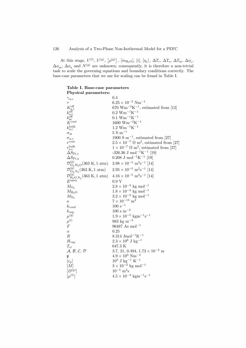
126 Analysis of a Two-Phase Non-Isothermal Model for a PEFC
At this stage, U (l), U (g),£ρ(g)
¤, [
·mH2O], [i], [ηc] , ∆Tc, ∆Ta, ∆Tm, ∆φc,
∆φm, ∆φa and N (g) are unknown; consequently, it is therefore a non-trivialtask to scale the governing equations and boundary conditions correctly. Thebase-case parameters that we use for scaling can be found in Table I.
Table I. Base-case parametersPhysical parameters:γa,c 0.4τ 6.25× 10⁻² Nm−1Keffa,c 670 Wm−2K−1, estimated from [12]
keffa,c 0.2 Wm−1K−1
keffm 0.1 Wm−1K−1
Kcont 1600 Wm−2K−1
kbulka,c 1.2 Wm−1K−1
σm 5 S m−1
σa,c 1900 S m−1, estimated from [27]rcont 2.5× 10⁻⁷ Ω m2, estimated from [27]rbulka,c 1× 10⁻⁷ Ω m2, estimated from [27]∆SPt,c -326.36 J mol−1K−1 [19]∆SPt,a 0.208 J mol−1K−1 [19]D(g)O2,H2O
(363 K, 1 atm) 3.98× 10⁻⁵ m2s−1 [14]D(g)O2,N2
(363 K, 1 atm) 2.95× 10⁻⁵ m2s−1 [14]D(g)H2O,N2(363 K, 1 atm) 4.16× 10⁻⁵ m2s−1 [14]Eopen 0.9 VMO2 2.8× 10⁻² kg mol−1MH2O 1.8× 10⁻² kg mol−1MN2 3.2× 10⁻² kg mol−1κ 7× 10⁻¹³ m2kcond 100 s−1
kvap 100 s m−2
µ(g) 1.9× 10⁻⁵ kgm−1s−1ρ(l) 983 kg m−3
F 96487 As mol−1
α 0.25R 8.314 Jmol−1K−1
Hvap 2.3× 10⁶ J kg−1Tcr 647.3 KA, B, C, D 3.7, 21, 0.494, 1.73× 10⁻⁴ mp 4.9× 10³ Nm−2[cp] 103 J kg−1 K−1
[M ] 3× 10⁻² kg mol−1[D(g)] 10−5 m2s[µ(l)] 4.5× 10⁻⁴ kgm−1s−1

E. Birgersson, M. Noponen and M. Vynnycky 127
The relevant length scale, l, is w/2 in the porous backing of the cathodeand anode, with l = hm in the membrane. Since the flow field compriseschannels (II, VII) and shoulders (I, VI) the length scale in the porous backingshould reflect the ratio of channel half-width to shoulder half-width; in our casewI,VI = wII,VII = w/2. For a net-type flow field, e.g. as in [13], the appropriatelength scale would be the height of the porous backing.
Table I. Operating conditions:p(g)0 101.325× 10³ Pahin 95%T cool 333 Khm 5× 10⁻⁵ m, estimatedha,c 3× 10⁻⁴ m, estimatedws 5× 10⁻⁴ mw 10−3 mEcell 0.6 Vφa,0 0 Vs0 0Cathode electrokinetics:ζ1 581 Am−2 [13]ζ2 30.6 V−1 [13]
8.1. Dimensionless numbers. In addition, the following dimensionlessnumbers, which will appear in the nondimensionalized form of the governingequations, are defined as follows:
Pe(mass) =U (g)l£D(g)
¤ , Pe(heat) = U (g)£ρ(g)
¤l [cp]
keff, Ca(g) =
µ(g)U (g)l
|p|κ ,
Ca(l) =[µ(l)]U (l)l
|p|κ , Gr(l) =µ(l)U (l)
ρ(l)gκ, Gr(g) =
µ(g)U (g)
ρ(g)gκ, O =
4F [ηc]
T cool |∆SPt| ,
H =Hvap l
2[·mH2O]
keff∆Tc, J =
σ(∆φ)2
keff∆T, T =
∆T
T cool, P = [µ(g)]U (g)l
p(g)0 κ
.
Here Pe(mass), Pe(heat), Ca(g,l) and Gr(g,l) are the Peclet numbers for massand heat transfer, and the capillary and gravitary numbers for gas and liquidphases, respectively. Pe(mass) and Pe(heat) give the ratio of bulk mass transferto diffusive mass transfer and heat convection to heat conduction, respectively;the capillary number gives the ratio of the viscous pressure drop to the capillarypressure; the gravitary number gives the ratio of the viscous pressure drop tothe gravitational pressure. O describes the magnitude of heat generated fromthe overpotential in relation to the heat due to entropy change, and H and Jgive the ratio of heat of condensation and ohmic heating to the heat conduction,respectively. T and P show the effect of the changes in the temperature and gaspressure, as we will see later in the analysis. Note that for J and T : ∆φ = ∆φcand ∆T = ∆Tc in the porous backing (cathode); ∆φ = ∆φa and ∆T = ∆Ta
128 Analysis of a Two-Phase Non-Isothermal Model for a PEFC
in the porous backing (anode); ∆φ = ∆φm and ∆T = ∆Tm in the membrane.For brevity, we have also referred to the effective heat conductivity and electricconductivity as keff and σ in the nondimensional parameters above, implyingkeff , σ = (keffc , σc in the porous backing (cathode); keffa , σa in the porous backing(anode); keffm , σm in the membrane).
Dropping the tildes, we consider the governing equations for the cathode,membrane and anode in turn:
8.2. Cathode.
∇p(g) = −v(g)
κ(g)rel
− ρ(g)ey
Gr(g), (64)
∇ · (ρ(g)v(g)) = − [·mH2O]l
U (g)£ρ(g)
¤ ·mH2O, (65)
∇ · v(l) =[·mH2O]l
U (l)ρ(l)·mH2O, (66)
v(l) =κ(l)rel
Ca(l)µ(l)∇p(c) + Ca
(g)
Ca(l)κ(l)rel
κ(g)relµ
(l)v(g) − κ
(l)rel
Gr(l)µ(l)(1− [ρ
(g)]
ρ(l)ρ(g))ey, (67)
∇ ·Ãρ(g)v(g)
"w(g)O2
w(g)H2O
#!+
[·mH2O]l
U (g)£ρ(g)
¤ · 0·mH2O
¸
=1
Pe(mass)∇ ·
Ãρ(g)γ
32 (1− s)D(g)
"∇w(g)O2
∇w(g)H2O
#!, (68)
∇2Φc = 0, (69)
Pe(heat)³c(g)p,O2
n(g)O2+ c
(g)p,H2O
n(g)H2O
+ c(l)p,H2O
v(l)´·∇θc = ∇2θc+H
·mH2O+J (∇Φc)
2 .
(70)In Eq. 70, we have taken N (g) = ρ(l)U (l), which is confirmed later.
To start determining the correct scales, we begin with two of the boundaryconditions at the cathode active layer (IV), Eqs. 20 and 21, which are now
ρ(g)v(g) = − [i][M ]
4F£ρ(g)
¤U (g)
icMO2 , (71)
v(l) =[i][M ]
4Fρ(l)U (l)ic(2 + 4α)MH2O. (72)
Thus, the velocity scales U (g,l) are simply
U (g) =[i][M ]
4F£ρ(g)
¤ , U (l) = [i][M ]
4Fρ(l),
and hence U (l) = U (g)£ρ(g)
¤/ρ(l), which implies that the scale for the interface
mass transfer in Eqs. 65, 66, 68, 70 is [·mH2O] = [i][M ]/(4lF ). Note, however,
E. Birgersson, M. Noponen and M. Vynnycky 129
that these scales for the phase velocities are only valid provided that the con-vection in the porous backing is governed by the reactions occurring in theactive layer, and that any forced convection, due to e.g. an interdigitated flowfield, is negligible by comparison.
The mass flux scale N (g), is also found from the active layer at the cathode.Eq. 22 is now "
n(g)O2
n(g)H2O
#· ey = −
[i][M ]
4FN (g)ic
µMO2
0
¶, (73)
from which we have N (g) = [i][M ]/(4F ).The temperature scale∆Tc is determined from the ORR at the active layer,
Eq. 24. In dimensionless form, this gives,µPe(heat)(c
(g)p,O2
n(g)O2+ c
(g)p,H2O
v(l)) · eyθc −∂θc∂y
¶IV+
=
l[i]T cool¯∆SPt
¯4Fkeffc ∆Tc
ic
³Tm θm|IV− + 1−Oηc
´+
µ−k
effm w/2
keffc hm
∆Tm∆Tc
∂θm∂y
¶IV−
,
(74)
whence ∆Tc = w/2[i]T cool¯∆SPt
¯/(4Fkeffc ), provided that Pe
(heat), Tm, O,keffm w/2keffc hm
∆Tm∆Tc
are no greater than O (1) ; we show later that these conditions areindeed satisfied.
The scale for the potential ∆φc is given by the boundary condition at theactive layer (IV), Eq. B.10
−∂Φc∂y
¯IV+
=[i]w/2
σc∆φcic, (75)
as ∆φc = [i]w/(2σc).Returning to the ideal gas law, Eq. 37, we have
ρ(g) =p(g)0 [M ]£
ρ(g)¤RT cool
µPp(g) + 1Tcθc + 1
¶M(g).
Thus, the density scale for the gas is£ρ(g)
¤= p
(g)0 [M ]/(RT
cool), provided thatPc, Tc are at most O (1) , which we will also show later.
8.3. Membrane. Now, we turn our attention towards the membrane,where we obtain
∇2θm + J (∇Φm)2 = 0, (76)
∇2Φm = 0. (77)
The scale for the potential drop can be inferred from the interface condition atthe cathode (IV), Eq. B.10,
− ∂Φm∂y
¯IV−
=[i]hm
σm∆φmic, (78)
130 Analysis of a Two-Phase Non-Isothermal Model for a PEFC
as ∆φm = [i]hm/σm.To find the temperature scale in the membrane, we return to the second
term on the RHS of Eq. 74, and require the heat conduction in the membraneto be of the same order of magnitude as that in the porous backing, i.e.
keffm w/2
keffc hm
∆Tm∆Tc
∼ O(1), (79)
whence the proper temperature scale is
∆Tm =keffc hmkeffm w/2
∆Tc. (80)
Assuming that the liquid velocity for the water transport in the membrane isof the same order of magnitude as in the porous backing of the cathode, we willbe able to estimate Pe(heat) (substitute [U (l)]ρ(l) = [U (g)][ρ(g)] in the definitionof Pe(heat)) for the membrane.
8.4. Anode. In the anode, we arrive at
∇2θa + J (∇Φa)2 = 0, (81)
∇2Φa = 0. (82)
The scale for the potential ∆φa can be found by combining the two boundaryconditions at the active layer (V), Eq. 28, which become
− ∂Φa∂y
¯V−
= − σm∆φmw/2
σa∆φahm
∂Φm∂y
¯V+
, (83)
in order to remove the contact resistance, which we shall treat separately. Thiscondition yields ∆φa = σmw/2∆φm/(hmσa), which, upon inserting ∆φm, gives∆φa = [i]w/(2σa).
The interface condition between the porous backing of the anode and themembrane, Eq. 30, which scales as
−∂θa∂y
¯V−
= −keffm ∆Tmw/2
keffa ∆Tahm
∂θm∂y
¯V+
, (84)
provides the temperature scale, namely ∆Ta = keffm ∆Tmw/(2keffa hm). ∆Tm in
turn depends on the temperature scale in the porous backing of the cathode,and inserting this expression for ∆Tm finally leads to ∆Ta = kc/ka∆Tc orsimply ∆Ta = ∆Tc (kc = ka).
8.5. Current density scale. So far, most of the scales that we havesecured in the porous backing of the cathode and anode as well as in themembrane contain the current density scale [i], i.e. most of the transportphenomena and corresponding dimensionless numbers depend on this scale.Returning to the current density expression, Eq. 62, and the definition of the
E. Birgersson, M. Noponen and M. Vynnycky 131
overpotential at the cathode, Eq. 63, these become after nondimensionalisation(N.B. Φm ≤ 0, Φc ≥ 0 )
[ηc]ηc = Ecell +∆φc Φc|IV + [i]rcont| z φs|IV
− (∆φm Φm|IV − 2[i]rcont −∆φa)| z φm|IV
−Eopen.
(85)such that
[i]ic = ζ1x(g)O2(1− s) exp
£ζ2(E
open −Ecell)¤exp [−ζ2∆φc Φc|IV]
exp [−ζ2∆φa] exp [−ζ2∆φm |Φm|IV|] exp£−3ζ2[i]rcont
¤. (86)
We can now extract the scale for the overpotential from Eq. 85 as
[ηc] = Eopen −Ecell −∆φc −∆φa −∆φm − 3[i]rcont, (87)
and the current density scale from Eq. 86 as
[i] = ζ1x(g)O2,0
exp£ζ2(E
open −Ecell)¤exp [−ζ2∆φc]
exp [−ζ2∆φa] exp [−ζ2∆φm] exp£−3ζ2[i]rcont
¤. (88)
The various contributions to the potential drop throughout the cell appear in[ηc] and the resulting current density scale [i]. Now, recalling the scales for thepotential drops,
∆φc =[i]w/2
σac, ∆φa =
[i]w/2
σa, ∆φm =
[i]hmσm
,
the current density scale reduces to
[i] = ζ1x(g)O2,0
exp£ζ2(E
open −Ecell)¤exp
¡−[i]ζ2
©3rcont .
+
·w
2σc+
w
2σa+
hmσm
¸¾¶(89)
We have here assumed that (1 − s) is a O(1) function, which as we shall seelater holds for case a-c. If the water is expected to have a leading order effecton the current, an additional scale should be introduced in Eq. 89 to accountfor this. As it stands, Eq. 89 is an implicit equation for [i]; however, referringto appendix A for the details, we arrive at
[i] ∼ − 1λlog
µlog (λµ)
λµ
¶,
where
µ = ζ1x(g)O2,0
exp£ζ2(E
open −Ecell)¤,
λ = ζ2
½3rcont +
·w
2σc+
w
2σa+
hmσm
¸¾.

132 Analysis of a Two-Phase Non-Isothermal Model for a PEFC
8.6. Magnitude of scales and dimensionless numbers. The scalesand dimensionless numbers and their magnitudes for case a are summarized inTables II and III, respectively. Note in particular the values of Pe(heat), Tm,O,
keffm w/2keffp hm
∆Tm∆Tp
and Pc, which are all small enough to ensure that our scalingsfor ∆Tc and [ρ(g)] are self-consistent; this provides a posteriori justification forthose scalings. To summarize the analysis thus far: the governing equationsdescribing conservation of mass, heat, charge, species and momentum with cor-responding boundary conditions, have been presented and nondimensionalised.A scale analysis has provided us with the proper scales to quantify the relativeimportance of different transport mechanisms in the porous backings of thecathode and anode, as well as in the membrane.
Table II. ScalesCurrent density:[i] −1/λ log (log (λµ) /(λµ)) ∼ 104 Am−2[ηc] Eopen −Ecell −∆φc −∆φa −∆φm − 3[i]rcont ∼ 0.17 Vµ ζ1x
(g)O2,0
exp£ζ2(E
open −Ecell)¤
∼ 106 Am−2λ ζ2 3rcont + [w/(2σc) + w/(2σa) + hm/σm] ∼ 3× 10⁻⁴ A−1m2Porous backing (Cathode):U (g) [i][M ]/(4F [ρ(g)]) ∼ 10−3 ms−1U (l) [i][M ]/(4F [ρ(l)]) ∼ 10−6 ms−1[ρ(g)] p
(g)0 [M ]/(RT cool) ∼ 1 kgm−3
[·mH2O] [i][M ]/(4Fw/2) ∼ 2 kgm−3s−1∆Tc w/2[i]T cool
¯∆SPt
¯/(4Fkeffc ) ∼ 8 K
∆φc [i]w/(2σc) ∼ 3× 10⁻³ VN (g) [i][M ]/(4F ) ∼ 10−3 kgm−2s−1Membrane:∆Tm keffc hm/(k
effm w/2)∆Tc ∼ 2 K
∆φm [i]hm/σm ∼ 0.1 VPorous backing (Anode):∆Ta kc/ka∆Tc (= ∆Tc) ∼ 8 K∆φa [i]w/(2σa) ∼ 3× 10⁻³ V
9. Numerics and validation
A commercial finite-element solver, FEMLAB 2.3 (see [30] for details), wasused to implement the model derived above. The heat transfer by convectionwas found to be negligible in the analysis, as will be discussed in the section onResults and discussion below, and therefore not implemented numerically. Thecomputational domain, the unit cell shown in Figure 1, was resolved with finiteelements, starting with a coarse mesh of around 900 elements. Consecutivemesh adaption of up to 2600 elements allowed for high resolution of the one-and two-phase interface. Mesh independence was ensured by comparing with

E. Birgersson, M. Noponen and M. Vynnycky 133
results obtained using a coarse mesh consisting of 900 elements, followed byseveral mesh adaptions, until the difference in computed current density wasbelow 1%.
Due to the high non-linearity and coupling of variables, the computationswere first carried out at low currents, and once convergence was obtained,the current was gradually increased. Obtaining a polarization curve requiredseveral hours with mesh adaption on a 2 GHz PC with 1 GB RAM. For someof the runs, it was found to be advantageous to solve for the model variablessequentially.
The model used here was validated previously for a net-type flow distribu-tor by Noponen et al. [13]. In that case, good agreement between experiments,conducted with a segmented cell, and the model was observed; there, however,only the normal direction (ey) had to be taken into account, which reduced thedimensionality of the model even further, whereas here, both the flow and thegeometry are fully two-dimensional.
Table III. Dimensionless parametersPorous backing (Cathode):Pe(heat) U (g)
£ρ(g)
¤w [cp] /(2k
effc ) ∼ 2× 10⁻³
Pe(mass) U (g)w/(2£D(g)
¤) ∼ 4× 10⁻²
Gr(l) µ(l)U (l)/(ρ(l)gκ) ∼ 0.1Gr(g) µ(g)U (g)/([ρ(g)]gκ) ∼ 2× 10³Ca(g) µ(g)U (g)w/(2 |p|κ) ∼ 10−3Ca(l) [µ(l)]U (l)w/(2 |p|κ) ∼ 10−5J σc(∆φc)
2/(keffc ∆Tc) ∼ 10−2O 4F [ηc]/(T
cool¯∆SPt
¯) ∼ 0.6
H Hvap(w/2)2[·mH2O]/(k
effc ∆Tc) ∼ 0.6
P [µ(g)]U (g)w/(2p(g)0 κ) ∼ 10−4
Tc ∆Tc/Tcool ∼ 2× 10⁻²
Membrane:Pe(heat) U (l)ρ(l)hm [cp] /k
effm ∼ 5× 10⁻⁴
J σm(∆φm)2/(keffm ∆Tm) ∼ 0.5
Tm ∆Tm/Tcool 5× 10⁻³
Porous backing (Anode):J σa(∆φa)
2/(keffa ∆Ta) ∼ 10−2
10. Results and discussion
The operating conditions were chosen to be the same as the conditions usedin the validation [13]. In all of the four cases (a-d), the operating conditionsand physical parameters are retained, except for the thermal conductivities andfor case d, the capillary pressure. The lengths of the current collector rib ws(boundary I and VI) and channel (boundary II and VII) are based on typicaldimensions found in a PEFC. The thickness of the porous backings, ha,c, are

134 Analysis of a Two-Phase Non-Isothermal Model for a PEFC
typical for a porous backing under compression. The MEA thickness, hm, is fora Gore Primea 5510. Simulations were carried out for cell potentials rangingfrom 0.9 V (Eopen) to 0.55 V.
First, the relative importance of the transport mechanisms will be exam-ined by returning to the dimensionless numbers and their magnitudes, afterwhich we shall study the numerically computed results for the four differentcases. Whilst discussing these, it will be instructive to recall the scalings andin particular to see how well they predict the behavior of the PEFC.
10.1. Heat transfer. The scale analysis has revealed that the Pecletnumber for heat transfer Pe(heat) ∼ 2 × 10⁻³ in the porous backing of thecathode and ∼ 5 × 10⁻⁴ in the membrane, implying that the main transportmechanism for heat transfer throughout the cell is conduction, i.e. the con-vective contribution is sufficiently small to be safely neglected. Given that theproperties in the anode are of the same magnitude as those in the cathode, thiswill also hold for the porous backing of the anode, as was assumed at the out-set. The bulk conductivity (case c) is much higher than the effective (case a,d),such that Pe(heat)(case c) < Pe(heat)(case a,d), whence convection is negligiblefor this case as well. At the cathode, the evaporation/condensation of water,will have a leading order effect on the total heat flux, since H ∼ 0.6.
10.2. Mass transfer in porous backings. The dominating mechanismis diffusion, since Pe(mass) ∼ 4 × 10⁻², and convection, originating from theactive layers, is negligible. The convective contribution can be increased byintroducing a flow field, e.g. having interdigitated channels, that induces astronger flow in the porous backing than the parallel channel arrangement wehave considered here.
10.3. Buoyancy in porous backings. The buoyancy in the gas phase,given by the gravitary number Gr(g) ∼ 2 × 10³, is negligible compared to theviscous pressure drop. For the liquid phase, Gr(l) ∼ 0.1, whence the buoyancy issomewhat larger than the viscous pressure drop. For the liquid phase, however,the capillary pressure constitutes an additional driving force, see Eq. 67; tofind the ratio between it and the gravitational force, we employ the gravillarynumber, defined as Gl(l) = ρ(l)gl/ |p| = Ca(l)/Gr(l) ∼ 10−4. This gives the ratioof the gravitational pressure to the capillary pressure, whence the buoyancy isfound to be negligible in the liquid phase compared to the capillary pressure.
10.4. Ohmic heating. The ohmic heating originating from the chargetransfer is a leading order effect in the membrane, where J ∼ 0.5, but is smallcompared to the heat conduction in the porous backings, since J ∼ 10−2. In themembrane, the high resistance of the polymer to charge transfer will thereforegive rise to appreciable heating, in contrast to the porous backing of the anodeand cathode.

E. Birgersson, M. Noponen and M. Vynnycky 135
10.5. Heat generation at the cathode active layer. At the activelayer of the cathode, the heat generated by the ORR is captured by the interfacecondition, Eq. 74, where the heat due to the overpotential is of the same orderof magnitude as the heat due to the entropy change (since O ∼ 0.6).
10.6. Thermal management. As was mentioned in the introduction,recent experimental findings [1, 12] suggest significant temperature gradientswithin the PEFC. This is also the case in our model, as can be seen in Figure2, where the temperature distributions for a cell potential of 0.6 V are depicted.
Figure 2. Temperature distributions (Ecell = 0.6 V): a) effective thermalconductivity (iav = 1080 mAcm−2); b) thermal contact resistances (iav = 1080mAcm−2); c) alternative capillary pressure expression (iav = 790 mAcm−2).
The temperature is highest at the cathode side of the membrane (boundaryIV), due to the exothermic ORR, and drops off towards the current collectorribs, which are kept at a constant temperature T cool = 60oC. At the interfacesto the channel (II, VII), the temperatures are higher for case a and d thanat the current collectors (I, VI), since the heat flux into the flow distributorchannels is assumed to be negligible compared to the heat flux to the currentcollector ribs, which are usually made out of a highly conductive material suchas graphite or steel. For case a, where the effective thermal conductivity isconsidered, the drop in temperature occurs throughout the porous backings

136 Analysis of a Two-Phase Non-Isothermal Model for a PEFC
and the membrane, amounting to a temperature difference of 4.5oC. In case c,where the heat conductivity comprises both a bulk and an interface conduc-tivity, most of the temperature loss takes place at the interfaces between thecurrent collectors and porous backings and porous backings and membrane.The overall temperature increase is here also 4.5oC: with ∼1oC increase acrossthe porous backings; ∼1oC increase at the interface between the current col-lectors and the porous backings; ∼2.5oC increase at the interface between theporous backing and the membrane on the cathode side and a correspondingincrease of ∼1oC at the anode. The temperature drops for case c are basedon the assumption that the heat interfacial contact conductivities mirror thosefound for the charge transfer, and can be expected to be larger or smaller de-pending on clamping pressure and on whether this assumption holds. For cased, with the alternative capillary pressure, the temperature distribution differsfrom the two aforementioned cases. Here, most of the temperature variationoccurs in the spanwise direction (ex), dropping from ∼65oC to ∼61oC. Theheat generated at the cathode active layer from the ORR depends on the localcurrent density, so the non-uniform temperature distribution for case d mostlikely originates from an uneven current density distribution along the activelayer of the cathode, whereas we surmise that the current density is more uni-form for case a and c. The anode side is somewhat warmer than the cathodeside for all three cases, which can be attributed to the cooling effect from thevaporization of the liquid water at the cathode side.
Taking the average temperature difference, defined as
∆Tav =1
w
Z w
0
T |IV− dx− T cool,
and depicted in Figure 3 for increasing currents, we see that the temperatureincrease for case a and c are almost identical. This is to be expected, sincethe effective heat conductivity represents an average of the bulk and interfaceconductivities. At 1000 mA cm−2, the temperature at the active layer of thecathode is ∼4.2oC higher than the current collector for case a and c, and ∼5oCfor case d, which is similar to the difference of 4-6oC that Vie [12] observedexperimentally at the cathode at this current, albeit for a cooling plate at ahigher temperature (∼70oC).
Recalling the temperature scales ∆Ta,c ∼ 8 K and ∆Tm ∼ 2 K from TablesII and III, we find that they are of the same order of magnitude as the computedtemperature increases of ∼5 K in the cathode and ∼1 K in the membrane. Thetemperature scale ∆Tc does not account for the cooling that originates fromthe vaporization of the liquid water, whence it overpredicts the temperatureincrease in the cathode. Nonetheless, it gives the proper scale of O(1-10)K.

E. Birgersson, M. Noponen and M. Vynnycky 137
0 200 400 600 800 1000 1200 14000
1
2
3
4
5
6
7
iav
/ mA cm-2
∆ Tav
/ °C
Figure 3. The temperature difference ∆Tav at the interface (boundary IV)between the porous backing and membrane on the cathode side and thecathode current collector (boundary VI) at varying current densities. (–):case a; (− ·−): case c; (· · ·): case d.
10.7. Water management. Turning our attention to the water manage-ment of the cathode, the liquid saturation distributions are depicted in Figure 4for a cell potential of 0.6 V. Several features are apparent; foremost is that thethree cases a-c all exhibit liquid saturations that are O(10−2), with a maximumof ∼ 10%, in stark contrast to case d, with saturations that exceed 90%. For thefirst three cases, the liquid water removal is sufficiently fast to avoid flooding ofthe cathode, whereas for the latter, the capillary forces for the water removalare too weak, leading to a partially flooded active layer, causing a reductionin the current density and hence also in the heat production. This decrease inheat production leads to the decrease in temperature in the spanwise directionthat was observed in Figure 2c. For cases a-c, the capillary pressure is of theorder of 104 Nm−2, thus constituting a higher driving force for the liquid waterthan for case d, where the capillary pressure is around 40 Nm−2. The liquidsaturation levels are similar in case b and c and somewhat higher than for casea; this stems from the similarity in the temperature distributions, since thetemperature in the cathode for case c is close to the cooling temperature ofthe current collector, 60oC, which is also the temperature for the isothermalcase, b. The overall lower temperature in the cathode for cases b and c alsoresult in a somewhat increased amount of liquid water compared to case a.

138 Analysis of a Two-Phase Non-Isothermal Model for a PEFC
Temperature, liquid saturation and current density profiles over the electrodeboundaries are reasonably homogeneous when the base case Leverett functionis used (cases a-c). This indicates that the water transfer profile through themembrane fairly independent of position, making the use of a constant waterdrag coefficient feasible. However, conditions on the electrode are drasticallychanged when the alternative expression for the capillary pressure is considered(case d): even though the electrode is severely flooded under the rib, the liquidsaturation drops to 10% at the section of the electrode that lies below the chan-nel. In this case, the use of a constant water drag coefficient is questionable.
Figure 4. Liquid saturation distributions (Ecell = 0.6 V): a) effectivethermal conductivity (iav = 1080 mAcm−2); b) isothermal (iav = 1080Acm−2); c) thermal contact resistances (iav = 1080 mAcm−2); d) alternativecapillary pressure expression (iav = 790 mAcm−2).
Proceeding to study the average liquid saturation at the active layer of thecathode (boundary IV), sav, defined as
sav =1
w
Z w
0
s|IV dx,
and shown in Figure 5 for increasing current densities, we find that sav is similarfor cases a-c and stays below 10% for the current densities considered. At 1000mAcm−2, case a displays an average liquid saturation of 6%, somewhat less than

E. Birgersson, M. Noponen and M. Vynnycky 139
for case b and c, with 7%, due to the higher overall temperature in the porousbacking of the cathode for case a, as compared to case b and c. The alternativecapillary expression, investigated in case d, behaves differently, displaying amaxima of around 45% at ∼ 800 mAcm−2 before apparently decreasing. Thehigh amount of liquid water for this case constitutes a high resistance to theoxygen transfer to the active layer of the cathode.
0 200 400 600 800 1000 1200 14000
0.05
0.1
0.15
0.2
0.25
0.3
0.35
0.4
0.45
0.5
iav
/ mA cm-2
s av
Figure 5. The average liquid saturation sav at the interface (boundary IV)of the porous backing and the membrane on the cathode for varying currentdensities. (–): case a; (· · ·): case b; (− ·−): case c; (−−): case d.
The disparity between the resulting amount of liquid water for the twodifferent capillary pressures requires ex situ experiments to determine the two-phase properties of the various components of the PEFC, especially in termsof capillary pressures and relative permeabilities. We can, however, based onthe flooding that arises in case d, infer that such low capillary forces are notdesirable from the point of view of water management.
Before addressing the final issue of cell performance, we will return to thescale analysis with a view to predicting the amount of liquid water from thescales alone. The removal of liquid water produced by the ORR at the activelayer of the cathode and due to the water transport through membrane is givenby Eq. 67. Here, the liquid velocity on the LHS is O(1) and has to balancewith at least one of the driving forces on the RHS, comprising capillary drivenflow, friction between the phases and buoyancy. The first term on the RHS,the capillary pressure term, is O(κ(l)rel/Ca
(l)) ∼ 105s3 (N.B. κ(l)rel = s3); the
second term on the RHS, the friction between the liquid and the gas phase, is

140 Analysis of a Two-Phase Non-Isothermal Model for a PEFC
O(κ(l)relCa
(g)/κ(g)relCa
(l)) ∼ 102s3 (κ(g)rel ∼ 1 for s . 10−1); the final term on the
RHS, the buoyancy term, is O(κ(l)rel/Gr(l)) ∼ 10s3. Clearly, the capillary term is
the dominating transfer mechanism for the liquid phase, whence we are requiredto balance it with the LHS: O(1) ∼ O(κ
(l)rel/Ca
(l)), thus κ(l)rel = s3 ∼ Ca(l) andfinally s ∼ 3
pCa(l) ≈ 2%. The scale analysis was conducted for a cell voltage
of 0.6 V, and the current density scale was found to be 1000 mAcm−2, whencewe are underpredicting the amount of liquid water in the cathode, 6-7% for thecomputed cases a-c. Nonetheless, the magnitude of O(10−2 − 10−1) is correct.Now, for the alternative capillary pressure, we find that Ca(l) ∼ 10−2 (p ∼ 40Nm−2), such that both terms on the RHS, the capillary driven and frictionbetween the liquid and gas phase, are of the same order of magnitude. Theyboth yield s ∼ 20%, once again falling below the computed liquid saturationof 45%, but still of the same correct order of magnitude (O(10−1 − 1)).
10.8. Cell performance. Thus far, we have examined the mass trans-fer, the thermal and water management of the cell, and now address the vitalcell performance. The overall cell behavior can be discerned from Figure 6,illustrating the polarization curves with and without iR-correction: the po-larization curve against the cell potential is the one that reflects the overallperformance of the cell, whilst the iR-corrected counterpart isolates the acti-vation overpotentials, in our case the cathode performance, since we take theanode activation overpotential to be negligible. The average current densities,iav, and iR-corrected potentials were obtained from
iav =1
w
Z w
0
icdx, E(iR-corrected) =1
w
Z w
0
(φs − φm)IV dx, (90)
respectively, along the cathode/membrane interface (boundary IV). Severalfeatures are apparent in the polarization curves, notably that cases a-c pre-dict almost identical fuel cell performance, both for the cell voltage and theiR-corrected voltage, and that case d performs worst. The lower performanceof the latter stems from the partial flooding of the active layer at the cathodeside, where the current density drops to almost zero due to the increased masstransfer limitations with respect to oxygen, whereas the first three all displaya liquid water content somewhat less than 10%, thus not restricting the accessof oxygen to the same extent. The different modes of heat transfer, rangingfrom an effective conductivity (a), over isothermal conditions (b), to the in-corporation of a bulk and interface conductivity (c), have a minor impact onthe cell polarization, mainly due to the fact that our expression for the currentdensity, ic, does not account for temperature changes. From the point of viewof catalyst utilization, the drop in current density along the active layer of thecathode that is observed for case d, is not desirable, since non-uniform currentdensity can be expected to influence degradation in time, thus affecting thelong-term performance of the cell.
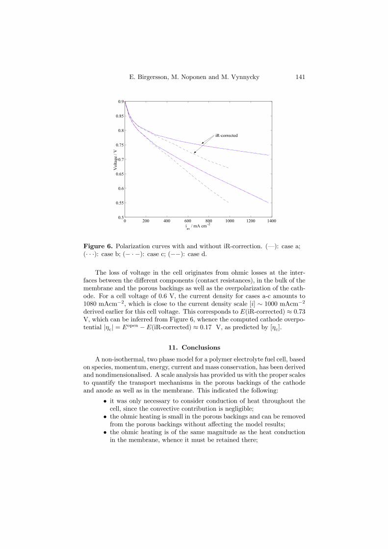
E. Birgersson, M. Noponen and M. Vynnycky 141
0 200 400 600 800 1000 1200 14000.5
0.55
0.6
0.65
0.7
0.75
0.8
0.85
0.9
iav
/ mA cm -2
Vol
tage
/ V
iR-corrected
Figure 6. Polarization curves with and without iR-correction. (–): case a;(· · ·): case b; (− ·−): case c; (−−): case d.
The loss of voltage in the cell originates from ohmic losses at the inter-faces between the different components (contact resistances), in the bulk of themembrane and the porous backings as well as the overpolarization of the cath-ode. For a cell voltage of 0.6 V, the current density for cases a-c amounts to1080 mAcm−2, which is close to the current density scale [i] ∼ 1000 mAcm−2derived earlier for this cell voltage. This corresponds to E(iR-corrected) ≈ 0.73V, which can be inferred from Figure 6, whence the computed cathode overpo-tential |ηc| = Eopen −E(iR-corrected) ≈ 0.17 V, as predicted by [ηc].
11. Conclusions
A non-isothermal, two phase model for a polymer electrolyte fuel cell, basedon species, momentum, energy, current and mass conservation, has been derivedand nondimensionalised. A scale analysis has provided us with the proper scalesto quantify the transport mechanisms in the porous backings of the cathodeand anode as well as in the membrane. This indicated the following:
• it was only necessary to consider conduction of heat throughout thecell, since the convective contribution is negligible;
• the ohmic heating is small in the porous backings and can be removedfrom the porous backings without affecting the model results;
• the ohmic heating is of the same magnitude as the heat conductionin the membrane, whence it must be retained there;

142 Analysis of a Two-Phase Non-Isothermal Model for a PEFC
• on the cathode side, diffusion of species is the dominating mecha-nism for species transfer, although this need only apply to a flow fieldwhich does not induce a forced flow in the porous backing, e.g. in-terdigitated channels. It should be noted, however, that although thehydrodynamics appears, at first sight, to decouple from heat, speciesand charge transfer, it is nevertheless present as a leading order effectthrough the saturation variable, s;
• buoyancy was also found to be negligible compared to capillary forcesfor the capillary pressure assumed in this study.
Three cases based on a) an effective heat conductivity, b) isothermal con-ditions and c) a two-fold conductivity comprising bulk and interface conduc-tivities, together with a fourth case, d) with an alternative capillary pressurehave been investigated numerically. The first three yielded similar results forthe water management, with a liquid saturation of around 10%, and the per-formance of the cell. The fourth deviated strongly due to the high liquid watercontent that was obtained at the active layer of the cathode, causing partialflooding, with a decrease in cell performance. In tandem with a discussionof these cases, the scales predicted gave good agreement with the computedquantities.
Acknowledgements
The financial support of the Swedish Foundation for Strategic Environmen-tal Research (MISTRA) and the Nordic Energy Research (NEFP) are gratefullyacknowledged. The work was done within the framework of the Jungner Cen-ter. In addition, the authors like to thank Dr. Jari Ihonen for his valuablecomments and suggestions related to the thermal and electrical properties ofgas diffusion layers.

E. Birgersson, M. Noponen and M. Vynnycky 143
Appendix A. Derivation of the current density scale
The current density scale is given by
[i] = ζ1x(g)O2,0
exp£ζ2(E
open −Ecell)¤exp
¡−[i]ζ2
©3rcont
+
·w
2σc+
w
2σa+
hmσm
¸¾¶. (A.1)
Now, with
µ = ζ1x(g)O2,0
exp£ζ2(E
open −Ecell)¤, (A.2)
λ = ζ2
½3rcont +
·w
2σc+
w
2σa+
hmσm
¸¾, (A.3)
we arrive at[i] = µ exp (−λ[i]) , (A.4)
where µÀ 1, λ¿ 1. We proceed by introducing log Y = λ[i], so that
Y log Y = λµ. (A.5)
Now, put Y = 1/Z, whence
Z
logZ= − 1
λµ. (A.6)
ThenlogZ − log (− logZ) ∼ − log (λµ) , (A.7)
whence, by combining Eq. A.6 and A.7,
Z ∼ log (λµ)λµ
. (A.8)
From the above, Z = exp(−λ[i]), which yields
exp (−λ[i]) ∼ log (λµ)λµ
, (A.9)
and finally
[i] ∼ − 1λlog
µlog (λµ)
λµ
¶. (A.10)
To verify [i], we substitute into (A.4)
− 1λlog
µlog (λµ)
λµ
¶exp
µ− log
µlog (λµ)
λµ
¶¶= µ.
The LHS reduces to
µ− µ
µlog (log (λµ))
log (λµ)
¶,
which is just µ at leading order.
144 Analysis of a Two-Phase Non-Isothermal Model for a PEFC
List of symbols
A, B, C, D constants for alternative capillary pressure,-,-,-,mB transformation tensorcp specific heat capacity, J kg−1K−1
Ca capillary numberD diffusion tensor, m2s−1eDij diffusion coefficients for molar diffusive flux, m2s−1
Dij diffusion coefficients for mass diffusive flux , m2s−1
Dij binary Maxwell-Stefan diffusion coefficients, m2s−1
ex, ey coordinate vectorsE potential, VF Faraday’s constant, As mol−1
g gravity vector, ms−2
Gr gravitary numberGl gravillary numberh height, mh relative humidityHvap heat of vaporization, J kg−1
H dimensionless numberi current density, A m−2
J(s) Leverett functionJ dimensionless numberk heat conductivity, W m−1K−1
kcond condensation rate constant, s−1
kvap evaporation rate constant, s m−2
K interfacial heat conductivity, W m−2K−1·mH2O interface mass transfer of water, kg m−3s−1
M (g) mean molecular mass of the gas phase, kg mol−1
Mi molecular mass of species i, kg mol−1
n number of electrons consumed in the ORR per oxygen moleculeni mass flux of species i, kg m−2s−1
N (g) scale for the mass fluxes, kg m−2s−1
O dimensionless numberp pressure, Nm−2
Pe Peclet numberP dimensionless numberr electric resitance, Ω m2
R gas constant, J mol−1 K−1
s liquid saturationS denominator for transformation of diffusion coefficients, m2s−1
S switch for interface mass transferT temperature, KT dimensionless numberv, u, v, U velocities, ms−1
V volume of the representative elementary volume, m3

E. Birgersson, M. Noponen and M. Vynnycky 145
w width, mwi mass fraction of species iW transformation tensorx, y coordinate, mxi molar fraction of species iX transformation tensorGreekα coefficient for water transport in the membraneγ porosityδij Kronecker delta∆T, ∆φ scales for temperature and potential∆SPt entropy change for the ORR, J mol−1 K−1
η overpotential, Vκ permeability, m2
λ parameter for current density scale, A−1m2
µ parameter for current density scale, Am−2
µ(k) dynamic viscosity of phase k, kg m−1 s−1
ρ density, kg m−3
σ electric conductivity, Sm−1
ζ1, ζ2 parameters in current density expression, Am−2, V−1
τ surface tension, Nm−1
φ potentialSubscripts0 referenceav averagea anodeb breakthroughc cathodecond condensationcr criticalH2O waterN2 nitrogenPt platinaO2 oxygenrel relatives solid phasevap vaporisation

146 Analysis of a Two-Phase Non-Isothermal Model for a PEFC
Superscriptsbulk bulk propertyc capillarycont contactcool coolingeff effectiveg gasheat heatk phase kl liquidmass massopen opensat saturation
Bibliography
[1] J. Ihonen, Development of Characterisation Methods for the Components of the PolymerElectrolyte Fuel Cell, dissertation, KTH, Sweden (2003).
[2] W. He, J. S. Yi and T. V. Nguyen, AIChE J., 10, 2053 (2000).[3] D. Natarajan and T.V. Nguyen, J. Electrochem. Soc., 148, A1324 (2001).[4] L.B. Wang, Nobuko I. Wakayama and Tatsuhiro Okada, Electrochemistry Communica-
tions, 4, 584 (2002).[5] L. You and H. Liu, Int. J. Heat Mass Transfer, 45, 2277 (2002).[6] Z.H. Wang, C.Y. Wang and K.S. Chen, Journal of Power Sources, 94, 40 (2001).[7] N. Djilali and D. Lu, Int. J. Therm. Sci., 41, 29 (2002).[8] G. J. M. Janssen, J. Electrochem. Soc., 148, A1313 (2001).[9] M. Wöhr, K. Bolwin, W. Schnurnberger, M. Fischer, W. Neubrand and G. Eigenberger,
Int. J. Hydrogen Energy, 23, 213 (1998).[10] T. Berning and N. Djilali, J. Electrochem. Soc., 150, A1598 (2003).[11] S. Mazumder and J. V. Cole, J. Electrochem. Soc., 150, (2003) A1510.[12] P. J. S. Vie, Characterisation and Optimisation of the Polymer Electrolyte Fuel cell,
dissertation, NTNU, Norway (2001).[13] M. Noponen, E. Birgersson, J. Ihonen, M. Vynnycky, A. Lundblad, G. Lindbergh, Fuel
Cells, submitted (2003).[14] F. Jaouen, G. Lindbergh and G. Sundholm, J. Electrochem. Soc., 149, (2002) A437.[15] D. M. Bernardi, M. Verbrugge, AIChE J., 37, 1151 (1991).[16] T. F. Fuller, J. Newman, J. Electrochem. Soc., 140, 1218 (1993).[17] T. E. Springer, T. A. Zawodsinski, S. Gottesfeld, J. Electrochem. Soc., 138, 2334 (1991)
.[18] A. C. West, T. F. Fuller, J. Appl. Electrochem., 26, 557 (1996).[19] M. J. Lampinen and M. Fomino, J. Electrochem. Soc., 140, 3537 (1993).[20] D.R. Lide and H.P.R. Frederikse (eds.), in CRC Handbook of Chemistry and Physics,
78th edition, CRC Press LLC, USA (1997).[21] D. Gawin, C. E. Majorana and B. A. Schrefler, Mech. Cohesiv.-Frict. Mater., 4, 37
(1999).[22] M. Kaviany, in Principles of heat transfer in porous media, Springer-Verlag (1995).[23] M.J. Lampinen, in Kemiallinen termodynamiikka energiatekniikassa (written in
Finnish), Libella painopalvelu Oy, Finland (1996).[24] T. V. Nguyen, The Electrochemical Society Proceedings, 14, 222 (1999).[25] R. Taylor and R. Krishna, Multicomponent Mass Transfer, John Wiley & Sons, USA
(1993).[26] J. R. Welty, C. E. Wicks and R. E. Wilson, Fundamentals of Momentum, Heat, and
Mass Transfer, 3rd edition, John Wiley & Sons, USA (1984).[27] M. Mathias, J. Roth, J. Fleming and W. Lehnert, in Handbook of Fuel Cells, John Wiley
& Sons, Chapter 46, W. Vielstich, H. A. Gasteiger, A. Lamm, Editors, John Wiley &Sons, Ltd (2003).
[28] A. J. Appleby and F. R. Foulkes, Fuel cell handbook, p.22, Van Nostrand Reinhold(1989).
147

148 Analysis of a Two-Phase Non-Isothermal Model for a PEFC
[29] R. Hilfer and P.E. Øren, Transp. Porous Media, 22, 53 (1996).[30] FEMLAB 2.3, http://www.comsol.com.

Paper 4


A Two-Phase Non-Isothermal PEFC Model:Theory and Validation
M. Noponen1, E. Birgersson2, J. Ihonen3, M. Vynnycky2, A. Lund-blad3 and G. Lindbergh3
1Laboratory of Advanced Energy Systems, Helsinki University of Technology, P.O.Box 2200, FIN-02015 HUT, Finland2Department of Mechanics, FaxénLaboratoriet, The Royal Institute of Technology,SE-100 44, Stockholm, Sweden3Department of Chemical Engineering and Technology, Applied Electrochemistry,The Royal Institute of Technology, SE-100 44 Stockholm, Sweden
Abstract. A two-dimensional, non-isothermal, two-phase model of a polymerelectrolyte fuel cell (PEFC) is presented. The model is developed for conditions wherevariations in the streamwise direction are negligible. In addition, experiments havebeen conducted with a segmented cell comprising net flow fields. The experimentallyobtained current distributions were used to validate the developed PEFC model.The PEFC model includes species transport and phase change of water, coupledwith conservation of momentum and mass, in the porous backing of the cathode,and conservation of charge and heat throughout the fuel cell. The current densityin the active layer at the cathode is modelled with an agglomerate model. Goodagreement was obtained between the modelled and experimental polarization curves.A temperature difference of 3.3 C between the bipolar plate and active layer on thecathode, and a liquid saturation of close to 5.5 % at the active layer in the cathodewere observed at 1 A cm−2.
1. Introduction
Recent years have seen a growing interest in fuel cells due to their potentialto reduce both carbon dioxide and local emissions (NOx, SOx, VOC, particles).One of the most promising types, especially for automotive applications, is thepolymer electrolyte fuel cell (PEFC).
The basic fuel cell consists of two porous electrodes, termed the anodeand the cathode, separated by a proton conducting membrane, as illustratedin Figure 1. Adjacent to each electrode is a porous backing, which made of acomposite material, containing carbon cloth and a hydrophobic agent, such aspolytetrafluoroethylene. The electrodes are thin porous structures, comprisinga supported electrocatalyst, such as carbon-supported platinum, and an ioniccarrier, usually a hydrated perfluorinated sulfonic acid polymer. These elec-trodes are dispersed on the membrane, forming a structure known as membraneelectrode assembly (MEA).
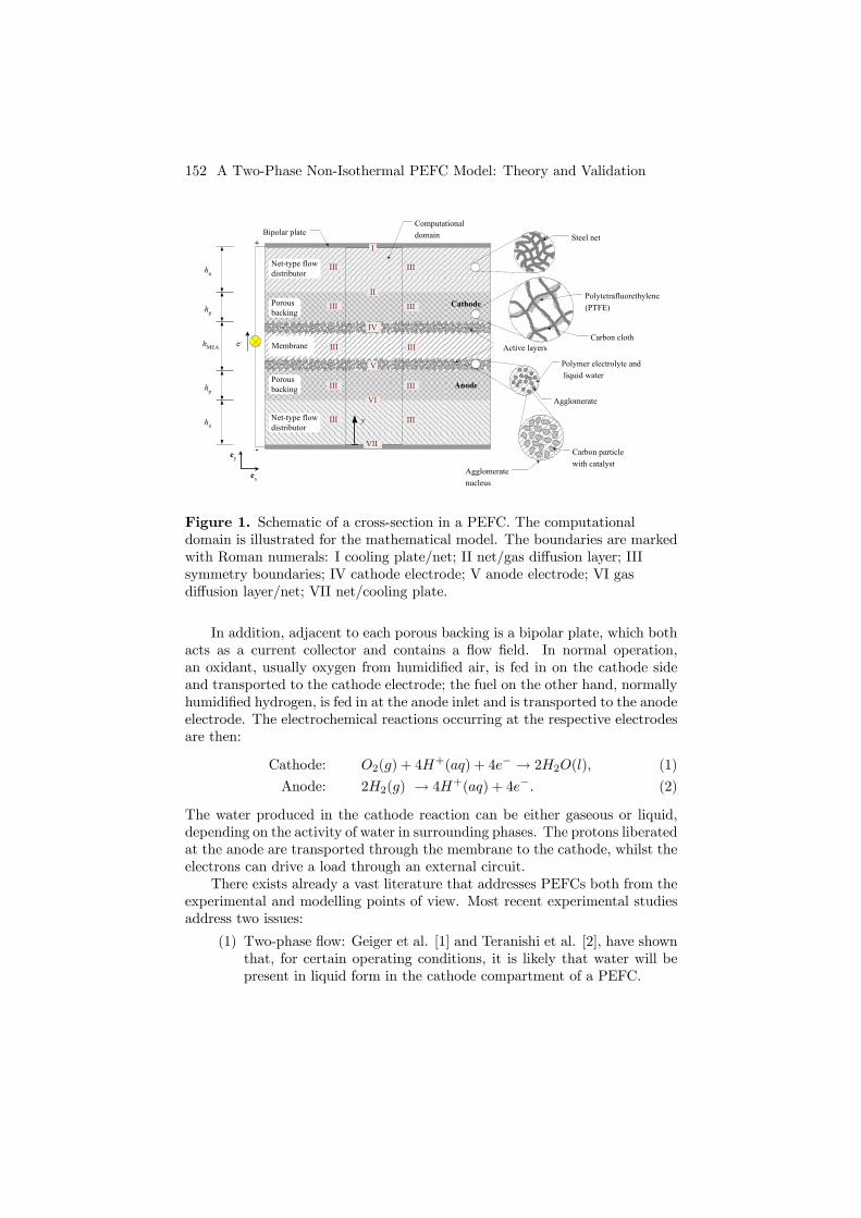
152 A Two-Phase Non-Isothermal PEFC Model: Theory and Validation
+
-
e- Membrane Active layers
Agglomeratenucleus
Porousbacking
Porousbacking Anode
Cathode
Polymer electrolyte and liquid water
Carbon particlewith catalyst
Agglomerate
Polytetrafluorethylene(PTFE)
Carbon cloth
Bipolar plate
Net-type flowdistributor
Net-type flowdistributor
I
II
IV
VI
VII
III III
III III
III III
III III
III III
V
yhn
hn
hp
hMEA
hp
Computationaldomain Steel net
ey
ex
Figure 1. Schematic of a cross-section in a PEFC. The computationaldomain is illustrated for the mathematical model. The boundaries are markedwith Roman numerals: I cooling plate/net; II net/gas diffusion layer; IIIsymmetry boundaries; IV cathode electrode; V anode electrode; VI gasdiffusion layer/net; VII net/cooling plate.
In addition, adjacent to each porous backing is a bipolar plate, which bothacts as a current collector and contains a flow field. In normal operation,an oxidant, usually oxygen from humidified air, is fed in on the cathode sideand transported to the cathode electrode; the fuel on the other hand, normallyhumidified hydrogen, is fed in at the anode inlet and is transported to the anodeelectrode. The electrochemical reactions occurring at the respective electrodesare then:
Cathode: O2(g) + 4H+(aq) + 4e− → 2H2O(l), (1)
Anode: 2H2(g) → 4H+(aq) + 4e−. (2)
The water produced in the cathode reaction can be either gaseous or liquid,depending on the activity of water in surrounding phases. The protons liberatedat the anode are transported through the membrane to the cathode, whilst theelectrons can drive a load through an external circuit.
There exists already a vast literature that addresses PEFCs both from theexperimental and modelling points of view. Most recent experimental studiesaddress two issues:
(1) Two-phase flow: Geiger et al. [1] and Teranishi et al. [2], have shownthat, for certain operating conditions, it is likely that water will bepresent in liquid form in the cathode compartment of a PEFC.
M. Noponen et al. 153
(2) Non-isothermal conditions: Vie [3] and Ihonen et al. [4] have shownthat thermal gradients can occur in PEFCs. In particular, Vie [3]measured a temperature difference of 4-5 oC between the gas chan-nel and the active layer at the cathode for a PEFC having a flowdistributor consisting of straight channels.
The need to operate a PEFC at high relative humidity levels or even attwo-phase conditions stems from the fact that the membrane conductivity isenhanced at these conditions. Too high liquid water content, however, couldresult in flooding of the electrodes, thus constituting a severe mass transferlimitation for oxygen on the cathode and hydrogen on the anode side. Numer-ous modelling studies have been carried out to investigate the water transferprocesses in a PEFC for cell optimization purposes. The models involve mul-ticomponent and multiphase mass transfer, heat transfer and electrochemicalreactions. Only a few models however exist where also the possibility for liq-uid water is accounted for. These resent models by Natarajan and Nguyen[5], Wang et al. [6], Wang et al. [7] and You and Liu [8] provide an insightinto the two-phase processes at the cathode side compartment of a PEFC andmodel by Djilali and Lu [9] even for the whole PEFC. Most of these models[5-8] assume isothermal conditions, while only Djilali and Lu [9] consider non-isothermal conditions, showing over 5 oC temperature difference between thecathode electrode and the cooling plate at 1 A cm−2. The model is howeverone dimensional and thus restricted to the cases where high stoichiometries areused.
A related issue concerns the validation of models themselves. For PEFCs,this is usually done against polarization curves via an averaged current forthe whole active region. However, whole cell polarization measurements areunable to capture any local gradients in concentrations or current productionin either the cell’s streamwise or spanwise directions. For this purpose, currentdistribution measurements could be a viable tool, even though the currentdistribution studies in polymer electrolyte fuel cells (PEFC) performed recentlyby many research groups [10-17] have seldom been used for model validation.The advantage of the segmented cell is that fuel cell models, ranging from one-to three-dimensional, can be validated.
The purpose of this paper, therefore, is to present a two-phase, non-isothermal model for a PEFC, and to validate it using via experiments ona segmented cell. The experimental setup and measurement procedure areintroduced in Section 2. The mathematical model, outlined in Section 3, is amodified version of the PEFC model derived by the authors [18]. The governingequations, boundary conditions, constitutive relations and electrokinetics aresummarized in appendices A to D. In our study [18], we used a flow distributorcomprising parallel channels, whereas here we consider a net flow field. Wesolve for two-phase mass, momentum and species transfer in the porous back-ing of the cathode and conservation of charge and heat throughout the fuelcell, i.e. in the membrane, net and anode as well. The computational domainis a cross-section of the PEFC, which limits the model to fuel cells run at high

154 A Two-Phase Non-Isothermal PEFC Model: Theory and Validation
stoichiometries, so as to avoid changes in oxygen and hydrogen concentrationalong the flow distributors. The results are presented and discussed in Section4. We finish with conclusions in Section 5.
2. Experiments
Current distribution measurements were conducted with a segmented cell,as illustrated in Figure 2.
Figure 2. (A) Structure of the segmented cell: a) current collector at thecathode; b) gasket for the cooling part; c) MEA (Gore Primea 5510) with gasdiffusion layers (CARBELTM); d) segmented flow field; e) segmented currentcollector; f) back plate for the segmented current collector; g) flow field forwater; h) gasket; i) endplate. The anode and cathode gaskets and the cathodeside steel net (flow field) are not illustrated. (B) Flow field plate with thesegment numbers. Badly operating segments are highlighted.
The three principal components of the cell comprise the segmented anodeside, the unsegmented cathode and the cooling system, based on water circu-lation. The advantage of segmenting the anode, and not the cathode, stemsfrom the fact that the electrode kinetics are much faster, and concentrationprofiles more uniform, at the anode side, resulting in only minor disturbancesin current distribution as compared to an unsegmented fuel cell.
The segmented current collector comprises of 4 spanwise and 8 streamwiseelectrically isolated segments (2e) of steel SS316 attached on a back plate (2f)made of the same material. The coordinates of a specific segment will begiven by (ξ, ψ), where ξ denotes the streamwise and ψ the spanwise position.Segments were electrically isolated from the back plate with a heat conductive
M. Noponen et al. 155
tape. A segmented platinum plated stainless steel SS2343 net was used asa flow distributor (2d). The porous backing, CARBELTM CL gas DiffusionMedia from W.L. Gore&Associates, Inc.(1c), and the the MEA, Primea 5510with 0.3 mgPt cm-2 loading at both sides from W. L. Gore&Associates, Inc.,(2c) were not segmented in the measurements. The cathode consists of thesame parts as the anode, with the important difference that no parts weresegmented.
The cell was tempered by circulating liquid water in a gold plated stainlesssteel net (2g) between the endplate (2i) and the segmented current collector(2e) on the anode and in a similar arrangement on the cathode side. The celldimensions are 90 mm in the streamwise direction and 60 mm in the spanwisedirection for the active layer. A more detailed description of the segmentedplate and measurement system can be found in [19].
Humidified air and hydrogen on the cathode and anode side, respectively,were used for the experiments. The cell was orientated vertically, with theanode and cathode gases entering from the top. The cell temperature wascontrolled by keeping the circulating cooling water at 60±1 oC. The dew pointtemperature of the humidified inlet gases was 60 oC and the stoichiometriesat the cathode and anode were 2.3 and 3.35, respectively. The measurementswere performed in galvanostatic mode. Ten measurement points were chosen,starting from low to increasingly higher currents. The fuel cell was allowed tostabilize at each current level for ten to twenty minutes, after which the currentfor each segment was recorded for an additional ten minutes. Then, the totalcell resistance was measured by means of current interruption method.
There were found to be three poorly operating segments: (3,4), (8,4) and(7,2), as shown in Figures 2 and 4. The segment (3,4) was short-circuited into(3,3). The other two segments, (8,4) and (7,2), had higher resistances thanthe other segments. It was shown earlier by Noponen et al. [20] that smalldeviations in segment resistances do not radically change the mass transfercharacteristics in the cell. Thus, it is feasible to use the segmented cell as avalidation tool.
3. Mathematical model
A two-dimensional, non-isothermal model has been derived by the authors[18] for a cross-section perpendicular to the flow direction for a polymer elec-trolyte fuel cell. The region solved for contained the porous backings and MEAof the anode and cathode, where the flow fields, serpentine or parallel channelson both sides were reduced to appropriate boundary conditions. The free flowpath of gaseous reactants and products in such parallel channels is limited tothe open channels, so that the land area between the channels is usually lessutilised. A flow field comprising a net, however, does not give rise to such landareas and the whole surface of the porous backing is in contact with the flowfield. Here, we will consider such a net flow field design. The computationaldomain is shown in Figure 1. Note that the introduction of a net reduces themodel to one length dimension, specified by the y-axis in Figure 1, since there

156 A Two-Phase Non-Isothermal PEFC Model: Theory and Validation
will be no changes in the spanwise direction. The boundary conditions aredenoted with roman numerals.
A brief overview of the modified version of the model derived by [18] willbe given in this section, with the governing equations, boundary conditions,constitutive relations and electrokinetics summarized in Appendices A to D.
We solve for two-phase conservation of mass, momentum and species inthe porous backing of the cathode and for conservation of heat and chargethroughout the fuel cell. The main features and approximations for the porousbacking of the cathode are:
• Species: The liquid is taken to be pure water, since the solubility ofoxygen and nitrogen are low in water. The gas phase consists of aternary mixture of nitrogen, oxygen and water, the transport of whichis modelled with Fick’s generalized law.
• Momentum: Conservation of momentum for both the liquid and gasphase is given by the generalized Darcy equation, where the mech-anism for the liquid transport is the mobility of the phases and thecapillary pressure.
• Mass: Conservation of mass is given by the continuity equation forboth the liquid and gas phase.
• Evaporation/condensation of water: The transport equations are mod-ified to account for the heat and mass transfer between the gas andliquid phase.
For the whole computational domain:
• Heat: The heat transfer equation takes conduction, evaporation andohmic heating into account. The resistance to heat conduction is ac-counted for by an effective heat conductivity, which represents thebulk and interfacial resistances. In [18], the interface resistance toheat transfer is investigated. Note that the heat conductivity in theporous backing of the cathode is dependent on the liquid saturation;this was not modelled here, since we use an effective heat conductiv-ity, estimated from in situ measurements by [3]. Furthermore, we as-sume here that the heat from the ORR includes the reversible entropyproduction and heat from the overpotentials, but not the energy dif-ference between open circuit and reversible cell potentials. The “opencircuit” effect was omitted because it is widely believed the differencein open circuit potential and reversible potential is caused by impuri-ties on the platinum surfaces and gas leakages through the membrane,phenomena that both produce less heat than the ORR reaction.
• Charge: Conservation of charge and Ohm’s law is considered.• Electrokinetics: The active regions (IV and V) are reduced to interfaceconditions, where the agglomerate model of [21] is implemented onthe cathode side (IV) and the potential difference at the anode (V) istaken to be negligible. The contact resistances between the current

M. Noponen et al. 157
collectors and nets, as well as between the nets and porous backings,are accounted for.
• Membrane: The membrane is assumed to be fully hydrated, and aconstant water transfer coefficient is assumed for the total water flux.The Gore membrane in this study differs from Nafion; since it is notwell characterized, in terms of transfer properties, there is little pointin using a more sophisticated model that would take into accountwater transfer by diffusion, hydraulic pressure and migration.
The governing equations, together with the constitutive relations and ap-propriate boundary conditions, constitute a highly non-linear coupled systemof equations that must be solved numerically.
4. Numerics
A commercial finite-element based solver, FEMLAB 2.3 (see [22] for de-tails), was used to implement the model. The unit cell, see Figure 1, wasresolved with finite elements. Consecutive mesh adaptation allowed for highresolution of the one- and two-phase interface, where steep gradients in liquidsaturation occur. Mesh independence was ensured by comparing with a coarsemesh, followed by several mesh adaptations, until the difference in currentdensity compared to the previous run was lower than 1%.
Due to the high non-linearity and coupling of variables, the computationswere first carried out at low current densities, and once convergence was ob-tained, the current was gradually increased. For some of the runs, it was anadvantage to solve for the dependent variables sequentially. The operating andphysical parameters for the base case are given in Table 1.

158 A Two-Phase Non-Isothermal PEFC Model: Theory and Validation
Table I. Base-case parametersPhysical parameters:γp 0.4τ 6.25×10⁻² Nm−2θ 0keffa,c 0.2 Wm−1K−1, estimated from [3]keffm 0.1 Wm−1K−1
keffn 1 Wm−1K−1
σm 5 S m−1
σc,a 500 S m−1
σn 105 S m−1
∆SPt,c -326.36 J mol−1K−1 [30]∆SPt,a 0.208 J mol−1K−1 [30]D(g)O2,H2O
3.98× 10⁻⁵ m2s−1 at 363 K, 1 atm [21]
D(g)O2,N22.95× 10−5 m2s−1 at 363 K, 1 atm [21]
D(g)H2O,N2 4.16× 10⁻⁵ m2s−1 at 363 K, 1 atm [21]Eopen, Ereversible 0.9 V, 1.23 VMO2 2.8× 10⁻² kg mol−1MH2O 1.8× 10⁻² kg mol−1MN2 3.2× 10⁻² kg mol−1κ 7× 10⁻¹³ m2kcond, kvap 100 J m−3s, 100 s m−2
µ(g) 1.9× 10⁻⁵ kgm−1s−1µ(l) 4.7× 10⁻⁴ kgm−1s−1 at 363 K, 1 atmρ(l) 983 kg m−3
F 96487 As mol−1
α 0.25R 8.314 Jmol−1K−1
rcontact 2.5× 10⁻⁷ Ω m2Hvap 2.3× 10⁶ J kg−1Tcr 647.3 KOperating conditions:p0 1 atmhin 95%Tcool 60ChMEA, hp, hf 5× 10⁻⁵ m, 3× 10⁻⁴ m, 5× 10⁻⁴ mEc,0, Ea,0 0.6 V, 0 Vs0 0Agglomerate model parameters and anode current expression:ζ1 581 Am−2
ζ2 30.7 V−1
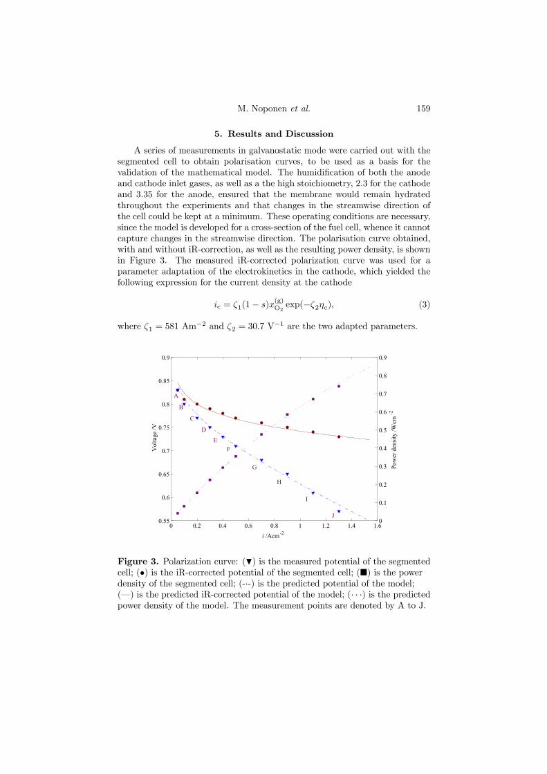
M. Noponen et al. 159
5. Results and Discussion
A series of measurements in galvanostatic mode were carried out with thesegmented cell to obtain polarisation curves, to be used as a basis for thevalidation of the mathematical model. The humidification of both the anodeand cathode inlet gases, as well as a the high stoichiometry, 2.3 for the cathodeand 3.35 for the anode, ensured that the membrane would remain hydratedthroughout the experiments and that changes in the streamwise direction ofthe cell could be kept at a minimum. These operating conditions are necessary,since the model is developed for a cross-section of the fuel cell, whence it cannotcapture changes in the streamwise direction. The polarisation curve obtained,with and without iR-correction, as well as the resulting power density, is shownin Figure 3. The measured iR-corrected polarization curve was used for aparameter adaptation of the electrokinetics in the cathode, which yielded thefollowing expression for the current density at the cathode
ic = ζ1(1− s)x(g)O2exp(−ζ2ηc), (3)
where ζ1 = 581 Am−2 and ζ2 = 30.7 V
−1 are the two adapted parameters.
0 0.2 0.4 0.6 0.8 1 1.2 1.4 1.60.55
0.6
0.65
0.7
0.75
0.8
0.85
0.9
i /Acm-2
Vol
tage
/V
0
0.1
0.2
0.3
0.4
0.5
0.6
0.7
0.8
0.9
Pow
er d
ensi
ty /W
cm-2
E
B
C
D
F
G
H
I
J
A
Figure 3. Polarization curve: (H) is the measured potential of the segmentedcell; (•) is the iR-corrected potential of the segmented cell; (¥) is the powerdensity of the segmented cell; (-·-) is the predicted potential of the model;(–) is the predicted iR-corrected potential of the model; (· · ·) is the predictedpower density of the model. The measurement points are denoted by A to J.

160 A Two-Phase Non-Isothermal PEFC Model: Theory and Validation
This expression corresponds to regime 1 [21], see Appendix D, where theactive layer is governed by the Tafel kinetics and is first order in the oxygenconcentration. Even at high currents around 1.4 A cm−2, this current den-sity expression predicts no mass transfer limitations inside the agglomerates ofthe active layer on the cathode, which would correspond to regime 2, 3 or 4,implying an active layer which is well integrated with the porous backing andthe membrane and comprising small agglomerates. Note that the temperaturedependence is hidden within the adapted parameters. Figure 3 not only showsthe ability of the model to predict the iR-corrected behaviour, but also themeasured cell potential for the whole cell, including resistances. The contactresistances between the bipolar plates and the net, as well as between the netand the porous backings, constitute 9 % of the total resistance, the bulk re-sistances of the nets and porous backings 3 % and the membrane 88 % at acurrent of 1.5 A cm−2.
The validation of the model hinges on the measured currents remaininguniform in the streamwise direction. In addition, the net gives rise to an evendistribution of the reactants to the porous backing, whence the current shouldnot vary in the spanwise direction either. Figure 4 depicts the measured currentdensity from each segment in the fuel cell.
8 7 6 5 4 3 2 11 2 3 4
0
0.050.08
8 7 6 5 4 3 2 11 2 3 4
00.10.20.3
8 7 6 5 4 3 2 11 2 3 4
0
0.25
0.5
8 7 6 5 4 3 2 11 2 3 4
0
0.5
1
8 7 6 5 4 3 2 11 2 3 4
00.5
11.5
8 7 6 5 4 3 2 11 2 3 4
0
1
2
A Flow directionC
G
JI
E
i /A
cm-2
i /A
cm-2
i /A
cm-2
i /A
cm-2
i /A
cm-2
i /A
cm-2
Spanwise position Streamwise position
Spanwise position Streamwise position
Spanwise position Streamwise position Spanwise position Streamwise position
Streamwise positionSpanwise position
Spanwise position Streamwise position
Figure 4. Current density distributions of the segmented cell for themeasurements: A, C, E, G, I and J.
Apart from the poorly operating segments, discussed in Section 2 on exper-iments, the current density distribution can be considered uniform everywhere,
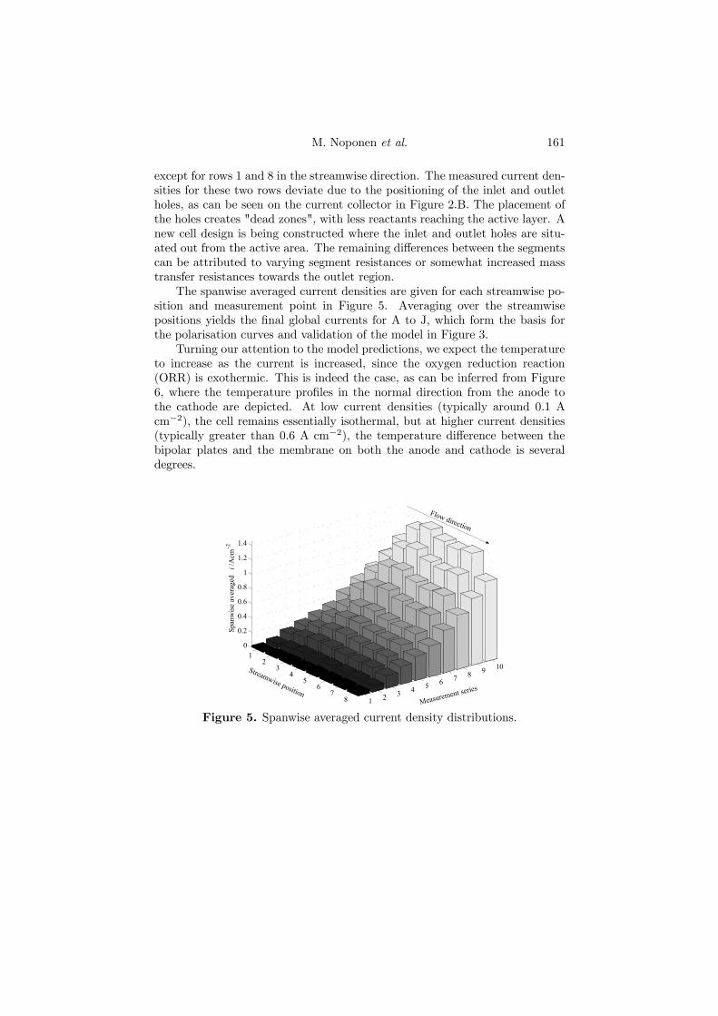
M. Noponen et al. 161
except for rows 1 and 8 in the streamwise direction. The measured current den-sities for these two rows deviate due to the positioning of the inlet and outletholes, as can be seen on the current collector in Figure 2.B. The placement ofthe holes creates "dead zones", with less reactants reaching the active layer. Anew cell design is being constructed where the inlet and outlet holes are situ-ated out from the active area. The remaining differences between the segmentscan be attributed to varying segment resistances or somewhat increased masstransfer resistances towards the outlet region.
The spanwise averaged current densities are given for each streamwise po-sition and measurement point in Figure 5. Averaging over the streamwisepositions yields the final global currents for A to J, which form the basis forthe polarisation curves and validation of the model in Figure 3.
Turning our attention to the model predictions, we expect the temperatureto increase as the current is increased, since the oxygen reduction reaction(ORR) is exothermic. This is indeed the case, as can be inferred from Figure6, where the temperature profiles in the normal direction from the anode tothe cathode are depicted. At low current densities (typically around 0.1 Acm−2), the cell remains essentially isothermal, but at higher current densities(typically greater than 0.6 A cm−2), the temperature difference between thebipolar plates and the membrane on both the anode and cathode is severaldegrees.
1 2 3 4 5 6 7 8 9 101
23
45
67
8
0
0.2
0.4
0.6
0.8
1
1.2
1.4
Span
wis
e av
erag
ed
i /A
cm-2
Streamwise positionMeasurement series
Flow direction
Figure 5. Spanwise averaged current density distributions.

162 A Two-Phase Non-Isothermal PEFC Model: Theory and Validation
0 0.2 0.4 0.6 0.8 1 1.2 1.4 1.6x 10⁻³
0
0.5
1
1.5
2
2.5
3
3.5
4
4.5
5
y/m
T-T
cool
/K
Anode side: net Anode side: porous backing
MEA
Cathode side: porous backing
Cathode side: net
i increasing
c)
e)
d)
b)
a)
VII VI V IIIV I
Figure 6. Temperature profiles in the fuel cell: a) i = 0.13 A cm−2; b) i =0.56 A cm−2; c) i = 0.86 A cm−2; d) i = 1.2 A cm−2; e) i = 1.4 A cm−2.
Figure 7. The liquid saturation in the cathode.
The temperatures are higher at the net/porous backing interface on theanode (VI) than at the cathode (II), since the liquid water from the membraneand the ORR is evaporated in the cathode, as it is transported from the activelayer (IV) to the net (II). This results in a cooling of the cathode, as can be seenfrom the change of slope in the temperature profile in the porous backing closeto the net (II). The evaporation is shown in Figures 7 and 8, where the liquid
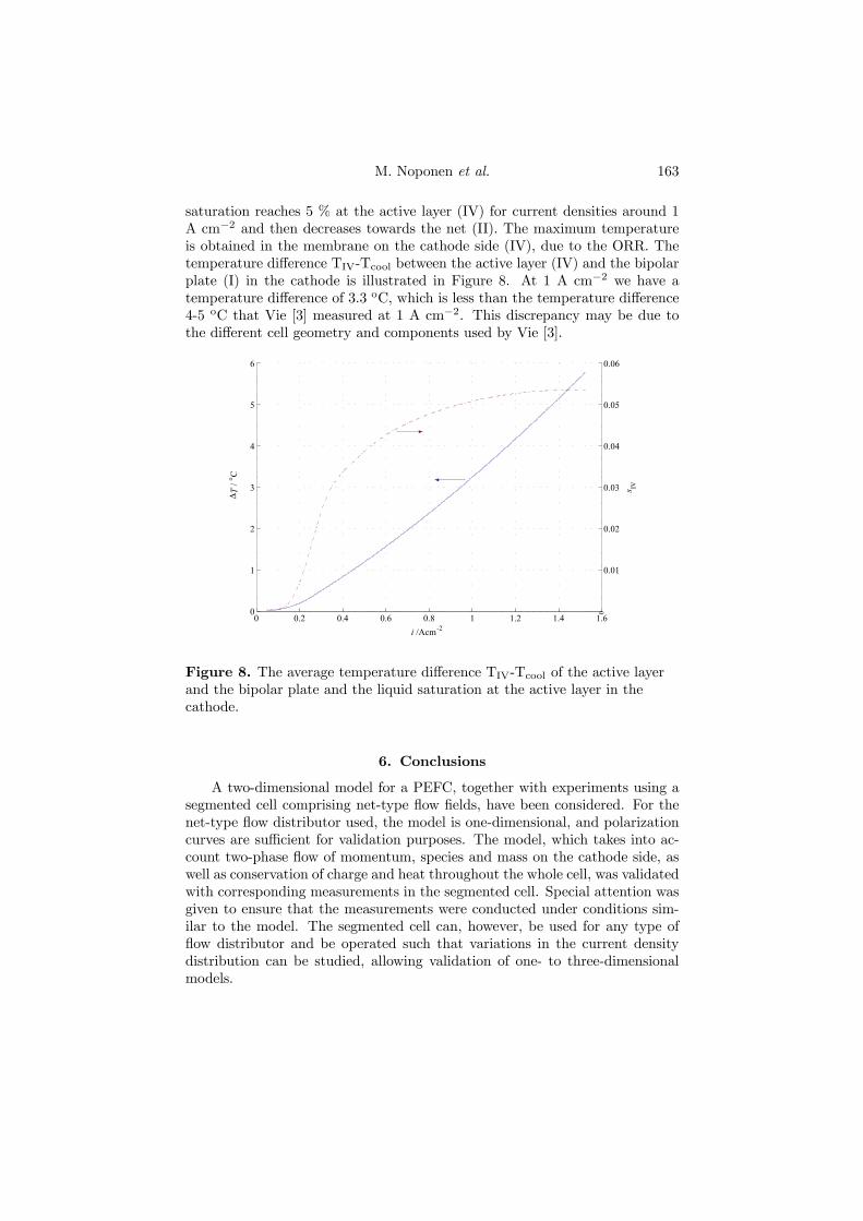
M. Noponen et al. 163
saturation reaches 5 % at the active layer (IV) for current densities around 1A cm−2 and then decreases towards the net (II). The maximum temperatureis obtained in the membrane on the cathode side (IV), due to the ORR. Thetemperature difference TIV-Tcool between the active layer (IV) and the bipolarplate (I) in the cathode is illustrated in Figure 8. At 1 A cm−2 we have atemperature difference of 3.3 oC, which is less than the temperature difference4-5 oC that Vie [3] measured at 1 A cm−2. This discrepancy may be due tothe different cell geometry and components used by Vie [3].
0 0.2 0.4 0.6 0.8 1 1.2 1.4 1.60
1
2
3
4
5
6
i /Acm-2
∆ T /
° C
s IV
0
0.01
0.02
0.03
0.04
0.05
0.06
Figure 8. The average temperature difference TIV-Tcool of the active layerand the bipolar plate and the liquid saturation at the active layer in thecathode.
6. Conclusions
A two-dimensional model for a PEFC, together with experiments using asegmented cell comprising net-type flow fields, have been considered. For thenet-type flow distributor used, the model is one-dimensional, and polarizationcurves are sufficient for validation purposes. The model, which takes into ac-count two-phase flow of momentum, species and mass on the cathode side, aswell as conservation of charge and heat throughout the whole cell, was validatedwith corresponding measurements in the segmented cell. Special attention wasgiven to ensure that the measurements were conducted under conditions sim-ilar to the model. The segmented cell can, however, be used for any type offlow distributor and be operated such that variations in the current densitydistribution can be studied, allowing validation of one- to three-dimensionalmodels.
164 A Two-Phase Non-Isothermal PEFC Model: Theory and Validation
The model predicts an increase in the temperature throughout the fuel cellas the current increases, with a maximum at the active layer on the cathodeside: at 1 A cm−2, a difference of 3.3 oC was observed between the bipolarplate and the active layer in the cathode. The liquid saturation in the cathodereached ~5.5 % at 1 A cm−2.
As a final note, it would have been of interest to run the cell up to floodingconditions, to see whether the derived model would be able to predict thisphenomenon. For this purpose, porous backings with poorer water managementproperties should be chosen, instead of the CARBELTM porous backings, whichwere shown by Ihonen et al. [4] to possess good water management properties.
Acknowledgements
The financial support of the Swedish Foundation for Strategic Environmen-tal Research (MISTRA) and the Nordic Energy Research (NEFP) are grate-fully acknowledged. The work was done within the framework of the JungnerCenter.
M. Noponen et al. 165
Appendix A. Governing Equations
In this paper, the superscripts (g) and (l) denote properties associated withthe gas and liquid phase, respectively, and (c) is for any quantity associatedwith the capillary pressure. All properties are intrinsic except for the velocity,mass fluxes and current density.
A.1 Cathode porous backing. We solve for the conservation of massand momentum of the liquid phase and gas phase:
∇ ·³ρ(g)v(g)
´= − ·
mH2O, (A.1)
∇ ·³ρ(l)v(l)
´=
·mH2O, (A.2)
∇p(g) = − µ(g)
κκ(g)rel
v(g), (A.3)
v(l) = mv(g) −D(c)∇s, (A.4)
where ρ(g,l) denote the phase densities, v(g,l) are the phase velocities,·mH2O is
the interface mass transfer of water between the gas and liquid phase, p(g,l) arethe phase pressures, µ(g,l) are the phase dynamic viscosities, κ is the perme-ability and κ
(g,l)rel are the relative permeabilities of the phases. The mobility m
and capillary diffusion D(c) are given by
m =κ(l)relµ
(g)
κ(g)relµ
(l), D(c) = −κκ
(l)rel
µ(l)dp(c)
ds. (A.5)
The conservation of charge together with Ohm´s law gives
∇2φs = 0; (A.6)
here, φs is the electric potential of the electric conductive phase. In addition,we solve for a ternary mixture of water, nitrogen and oxygen in the gas phase
∇ ·"n(g)O2
n(g)H2O
#+
·0
·mH2O
¸= 0, (A.7)
with the componental mass fluxes"n(g)O2
n(g)H2O
#= ρ(g)v(g)
"w(g)O2
w(g)H2O
#− ρ(g)γ
32 (1− s)D(g)
"∇w(g)O2
∇w(g)H2O
#, (A.8)
where D(g) is a multicomponent mass diffusion tensor, γ is the porosity, s isthe liquid saturation and w
(g)H2O
and w(g)O2
are the mass fraction of water andoxygen in the gas phase, respectively. The mass fraction of nitrogen in the gasphase can be found from
w(g)N2= 1− w
(g)H2O− w
(g)O2
. (A.9)

166 A Two-Phase Non-Isothermal PEFC Model: Theory and Validation
The heat transfer is given by
0 = ∇ ·¡keffc ∇T
¢+Hvap
·mH2O + σc (∇φs)
2 ; (A.10)
here T is the temperature, keffc is an effective thermal conductivity and Hvap
is the enthalpy of vaporization. The two last terms on the RHS of Eq. A.10account for the heat of vaporisation and ohmic heating.
A.2 Anode porous backing. On the anode side, we solve for conserva-tion of heat and together with conservation of charge and Ohm´s law
∇ ·¡keffa ∇T
¢+ σa (∇φs)
2= 0, (A.11)
∇2φs = 0, (A.12)
where φa is the electric potential.
A.3 Membrane. In the membrane, we solve for conservation of heat aswell as charge together with Ohm’s law, given by
∇ ·¡keffm ∇T
¢+ σm (∇φm)
2 = 0, (A.13)
∇2φm = 0, (A.14)
where φm is the potential in the ionic phase. The effective water flux throughthe membrane is modelled with a drag coefficient α.
A.4 Net. In the net, on both the anode and cathode side, we considerconservation of heat as well as charge with Ohm’s law
∇ ·¡keffn ∇T
¢+ σn (∇φs)
2= 0, (A.15)
∇2φs = 0, (A.16)
where φn is the potential in the net.
M. Noponen et al. 167
Appendix B. Boundary conditions
B.1 Cathode current collector/net interface (I). We require:
Tn = Tcool, -σn∂φs∂y
¯I−=
φs|I− −Ec,0rcontact
, (B.1)
where Tcool is the temperature of the current collector.
B.2 Cathode net/porous backing interface (II). We set the massfractions of oxygen and water , the gas pressure, and liquid saturation
w(g)O2= w
(g)O2,0
, w(g)H2O
= w(g)H2O,0
, p(g) = p(g)0 , s = s0, (B.2)
as well as requiring continuity of the temperature and the heat flux:
T |II− = T |II+ , keffc∂T
∂y
¯II−
= keffn∂T
∂y
¯II+
. (B.3)
At this interface, the contact resistance between the metallic net and the porousbacking yields
-σc∂φs∂y
¯II−
=φs|II− − φs|II+
rcontact, -σn
∂φs∂y
¯II+=
φs|II− − φs|II+rcontact
. (B.4)
B.3 Symmetry boundary conditions (III). At the right and left wallsin the whole cell, we specify symmetry boundary conditions:
cathode: u(g,l) = n(g)O2· ex = n(g)H2O · ex = 0,∇φs · ex = ∇T · ex = 0,
membrane: ∇φm · ex = ∇T · ex = 0,anode: ∇φs · ex = ∇T · ex = 0, (B.5)
B.4 Cathode active layer (IV). For the cathode, we treat the activelayer as an interface condition, whence the gaseous and liquid mass fluxes aregiven by:
ρ(g)v(g) · ey = − ic · eyMO2
4F, (B.6)
ρ(l)v(l) · ey =ic · ey4F
(2 + 4α)MH2O, (B.7)
and the componental fluxes in the gas phase by:"n(g)O2
n(g)H2O
#· ey = −
ic · ey4F
µMO2
0
¶. (B.8)
The temperature is taken to be continuous and the heat flux is given by:
T |IV− = T |IV+ , − keffc∂T
∂y
¯IV+
= ic · eyµ−T∆SPt,c
4F− ηc
¶− keffm
∂T
∂y
¯IV−
,
(B.9)where ηc is the cathode overpotential.
168 A Two-Phase Non-Isothermal PEFC Model: Theory and Validation
The potential is:
−σc∂φ
∂y
¯IV+
= ic · ey, − σm∂φ
∂y
¯IV−
= ic · ey, (B.10)
B.5 Anode active layer (V). We specify the continuity of current den-sity and a contineous potential:
−σm∂φs∂y
¯V+= −σa
∂φs∂y
¯V−
, φm|V+ = φs|V− . (B.11)
Here, the heat flux and continuity of temperature is:
T |V+ = T |V− , − keffm∂T
∂y
¯V+= −keffa
∂T
∂y
¯V−
. (B.12)
B.6 Anode net/porous backing interface (VI). We prescribe conti-nuity of the temperature and the heat flux:
T |VI+ = T |VI− , − keffa∂T
∂y
¯VI+
= −keffn∂T
∂y
¯VI−
. (B.13)
as well as the presence of an electric contact resistance:
-σa∂φs∂y
¯VI+
=φs|VI− − φs|VI+
rcontact, -σn
∂φs∂y
¯VI−
=φs|VI− − φs|VI+
rcontact. (B.14)
B.7 Anode current collector/net interface (VII). We require:
Tn = Tcool, -σn∂φs∂y
¯VII+
=Ea,0 − φs|VII+
rcontact. (B.15)

M. Noponen et al. 169
Appendix C. Constitutive relationships
The amount of liquid water in the cell is given by the liquid saturation s,defined as
s =γ(l)
γ, (C.1)
where γ(l) is the fraction of the total volume V occupied by the liquid phase
γ(l) =V(l)V . (C.2)
The constitutive relationship for the gas density is the ideal gas law
ρ(g) =p(g)M (g)
RT, (C.3)
where R is the gas constant and mean molecular mass of the gas phase isdefined as
M (g) =X
x(g)i Mi; (C.4)
here x(g)i is the mole fraction of species i.The density of the liquid water changes by - O(10−2 kg m−3) in the
temperature interval 300-363 K [23], allowing us to treat it as constant. Thedynamic viscosity of the gas phase can be taken as constant for the temper-atures considered here [24]. The dynamic viscosity for the liquid, however, ishighly temperature dependent [25]
µ(l) = 0.6612(T − 229)−1.562. (C.5)
The enthalpy of vaporisation [25]
Hvap = 2.672× 10⁵(Tcr − T )0.38, (C.6)
where Tcr is the critical temperature for water, can also be considered constantfor our temperature interval.
At this stage we do not have experimental data concerning the relevanttwo-phase parameters for the PEMFC, so the following empirical relationshipstaken from [7] will be used
J(s) = 1.417(1− s)− 2.120(1− s)2 + 1.263(1− s)3, (C.7)
p(c)(s) = τ cos θ³γκ
´ 12
J(s), (C.8)
κ(l)rel = s3, (C.9)
κ(g)rel = (1− s)3, (C.10)
where J(s) is a Leverett function, τ is the surface tension and θc is the wettingangle.

170 A Two-Phase Non-Isothermal PEFC Model: Theory and Validation
The interface mass transfer, due to condensation and evaporation of water,is defined as
·mH2O =
kcondγMH2Op(g)
RT
³x(g)H2O− xSatH2O
´S + kvapsp(g)
³x(g)H2O− xSatH2O
´(1−S),(C.11)
where
S =(0 , x
(g)H2O
< xSatH2O
1 , x(g)H2O≥ xSatH2O
; (C.12)
here,
xSatH2O(T, 1 bar) = 10(28.59051−8.2 log(T )+0.0024804T−3142.31/T ) (C.13)
is the saturation molar fraction of water taken from [26].The gas compositions at the porous backing/channel interfaces are deter-
mined by the relative humidity, defined as
h =x(g)H2O
xSatH2O
. (C.14)
On the cathode side, by keeping x(g)O2/x
(g)N2= 21/79 at the interface to the flow
channel (boundary VII) and utilizing x(g)O2+ x
(g)H2O
+ x(g)N2= 1, we arrive for a
given relative humidity at the mass fractions
x(g)H2O,0
= hxSatH2O, x(g)O2,0
=1− x
(g)H2O,0
1 + 79/21. (C.15)
The corresponding mass fractions can be found from
w(g)i =
x(g)i Mi
M (g). (C.16)
An expression for the diffusion tensor can be found from the diffusion coef-ficients eD(g)
ij for the molar diffusion flux, relative to a molar-averaged velocityframe, as [27]
eD(g)11 = D(g)O2,N2
(x(g)O2D(g)H2O,N2 + (1− x
(g)O2)D(g)O2,H2O
)/S, (C.17)eD(g)12 = x
(g)O2D(g)H2O,N2(D
(g)O2,N2
−D(g)O2,H2O)/S, (C.18)eD(g)
21 = x(g)H2O
D(g)O2,N2(D(g)H2O,N2 −D
(g)O2,H2O
)/S, (C.19)eD(g)22 = D(g)H2O,N2(x
(g)H2O
D(g)O2,N2+ (1− x
(g)H2O
)D(g)O2,H2O)/S, (C.20)
S = x(g)O2D(g)H2O,N2 + x
(g)H2O
D(g)O2,N2+ x
(g)N2D(g)O2,H2O
, (C.21)
where D(g)ij are the binary Maxwell-Stefan diffusion coefficients. Since we usethe mass diffusion flux relative to the mass-averaged velocity, the following
M. Noponen et al. 171
transformation is required:
D(g) = BWX−1 eD(g)XW−1B−1, (C.22)
B = δij − w(g)i
Ã1−
w(g)n x
(g)j
x(g)n w
(g)j
!, i, j = 1, 2, n = 3, (C.23)
X = x(g)i δij, i, j = 1, 2, (C.24)
W = w(g)i δij, i, j = 1, 2, (C.25)
where δij is the Kronecker delta. The binary Maxwell-Stefan diffusion coeffi-cients are corrected for pressure and temperature via
D(g)ij (T, p(g)) =p(g)0
p(g)
µT
T0
¶ 32
D(g)ij (T0, p(g)0 ), (C.26)
stemming from kinetic gas theory [28].
172 A Two-Phase Non-Isothermal PEFC Model: Theory and Validation
Appendix D. Electrokinetics at the active layers
The active layer is not resolved, but rather treated as a boundary condition.At the cathode, the volumetric current density iv, given by [21], is approximatedas
iv = Ai0,c¡1− γpol
¢(1− s) (1− γactive) exp
µ−αrFRT
ηc
¶Fc(g)O2
crefO2
(D.1)
whereAi0,c is the volumetric exchange current density in the agglomerates, γpolis the volume fraction of the polymer electrolyte in the agglomerate nucleus,c(g)O2= w
(g)O2
ρ(g)/MO2 is the molar concentration of oxygen, αr is the cathodictransfer coefficient for the ORR, n is the number of electrons consumed inthe ORR per oxygen molecule, ηc is the overpotential at the cathode (definednegative), and γactive is the volume fraction of pores in the active layer. F isthe nucleus effectiveness factor, defined as
F =3
Υr
µ1
tanh(Υr)− 1
Υr
¶, (D.2)
with Υ given by
Υ =
sAi0
¡1− γp
¢exp
¡−αrF
RT η¢
nFD, (D.3)
where D is an effective oxygen permeability in the agglomerates and r is theradius of the agglomerate nucleus. We omit the polymer film effectivenessfactor, since no experimental evidence hints at its presence. The impact ofliquid water on the current density is introduced via the linear term (1-s).The agglomerate model, without the term accounting for the liquid water, wasvalidated by [29] for a small PEFC with an area of 2 cm2. The total currentdensity is then locally given by ic = ivhactive. Jaouen et al. [21] discernedfour different regimes, where the Tafel slope doubles or even quadruples, andsubsequently supplied the experimental validation to support these [29]. Inregime 1, the active layer is controlled by Tafel kinetics and is first order inthe oxygen concentration. Regime 2 displays a doubling of the Tafel slope,due to the active layer being governed by Tafel kinetics and oxygen diffusionin the agglomerates, but still remains first order in the oxygen concentration.A doubling of the Tafel slope is observed in the third regime, where the activelayer is controlled by the Tafel kinetics, in addition to proton migration. Theoxygen dependence here is half-order. The final regime, the fourth, shows aquadrupling of the Tafel slope, and is attributable to an active layer controlledby Tafel kinetics, proton migration and oxygen diffusion in the agglomerates.The oxygen dependence is half-order, as in regime 3.
The overpotential at the cathode is given by
ηc = φs − φm −Eopen. (D.4)
at the interface between the porous backing and membrane on the cathodeside, region IV in figure 1.

M. Noponen et al. 173
On the anode, the fast kinetics of the hydrogen oxidation reaction (HOR),allows us to neglect the activtion overpotential, whence φm = φa at the interfacebetween the anode and membrane.

174 A Two-Phase Non-Isothermal PEFC Model: Theory and Validation
List of symbols
Ai0 Volumetric exchange current density, A m−3
B Transformation tensorc Molar concentration, mol m−3
Cp,i Heat capacity for species i, J kg−1K−1
D(c) Capillary diffusion, m2s−1
D Diffusion tensor, m2s−1eDij Diffusion coefficients for molar diffusive flux relativeto a molar-averaged velocity, m2s−1
Dij Diffusion coefficients for mass diffusive flux relativeto a mass-averaged velocity, m2s−1
Dij Binary Maxwell-Stefan diffusion coefficients, m2s−1
D Effective oxygen permeability in the agglomerates, mol m−1s−1
∆p Pressure drop, Nm−2
∆T Temperature drop, KE Potential, VF Faraday’s constant, As mol−1
F Nucleus effectiveness factor for the agglomerate modelh Height, mh Relative humidityHvap Heat of vaporization, J kg−1
i Current density, A m−2
iv Volume current density, A m−3
J(s) Leverett functionkeff Effective heat conductivity, W m−1K−1
kcond Condensation rate constant, J m−3skevap Evaporation rate constant, s m−2
K Interfacial heat conductivity, W m−2K−1
m Mobility of the liquid phaseM (g) Mean molecular mass of the gas phase, kg mol−1
Mi Molecular mass of species i, kg mol−1
n Number of electrons consumed in the ORR per oxygen moleculeni Mass flux of species i, kg m−2s−1
p, P Pressure, Nm−2
p Breakthrough pressure, Nm−2
r Radius of agglomerate nucleus, mR Gas constant, J mol−1 K−1
s Liquid saturationS Denominator for transformation of diffusion coefficients, m2s−1
T Temperature, Kv, U (g) Velocities, ms−1
V Volume of the representative elementary volume, m3
w Width, mwi Mass fraction of species iW, X Transformation tensorxi Molar fraction of species i

M. Noponen et al. 175
Greekα Coefficient for water transport in the membraneαr Cathodic transfer coefficient for the ORRγ Porosityδij Kronecker deltaη Overpotential, Vκ Permeability, m2
µ Dynamic viscosity, kg m−1 s−1
ρ Density, kg m−3
σ Electric conductivity, Sm−1
Υ Parameter for current density expressionφ Potential
Subscripts0 Referencea Anodec Cathodecond Condensationf Flow fieldH2O WaterMEA Membrane-electrode assemblyN2 Nitrogenp Porous backingpol Polymer electrolyte in the active layerPt PlatinumO2 Oxygenrel Relativevap VaporisationSuperscriptsc Capillaryg Gasl Liquidref References solid phasesat Saturation
Bibliography
[1] A.B. Geiger, A. Tsukada, E. Lehmann, P. Vontobel and G.G. Scherer, Fuel Cells,2, 82 (2002).
[2] K. Teranishi, S. Tsushima and S. Hirai, Thermal Science & Engineering, 10, 59(2002).
[3] P.J.S. Vie, Characterisation and optimisation of the polymer electrolyte fuel cell, Ph.D.thesis, NTNU, Trondheim (2002).
[4] J. Ihonen, M. Mikkola and G. Lindbergh, J. Electrochem. Soc., (2003) submitted.[5] D. Natarajan and T.V. Nguyen, J. Electrochem. Soc., 148, A1324 (2001).[6] L.B. Wang, N.I. Wakayama and T. Okada, Electrochem. Communications, 4, 584
(2002).[7] Z.H. Wang, C.Y. Wang and K.S. Chen, J. Power Sources, 94, 40 (2001).[8] L. You and H. Liu, Int. J. Heat and Mass Transfer, 45, 2277 (2002).[9] N. Djilali and D. Lu, Int. J. Therm. Sci., 41, 29 (2002).[10] D.J.L. Brett, S. Atkins, N.P. Brandon, V. Vesovic, N. Vasileiadis and A.R.
Kucernak, Electrochem. Commun., 3, 628 (2001).[11] S.J.C. Cleghorn, C.R. Derouin, M.S. Wilson and S. Gottesfeld, J. Appl. Elec-
trochem., 28, 663 (1998).[12] M.M. Mench, C. Y. Wang and M. Ishikawa, J. Electrochem. Soc., 150, A1052 (2003).[13] M. Noponen, T. Mennola, M. Mikkola, T. Hottinen and P. Lund, J. Power
Sources, 106, 312 (2002).[14] N. Rajalakshmi, M. Raja and K.S. Dhathathreyan, J. Power Sources, 112, 331
(2002).[15] J. Stumper, S.A. Campbell, D.P. Wilkinson, M.C. Johnson and M. Davis, Elec-
trochim. Acta, 43, (1998) 3773.[16] Ch. Wieser, A. Helmbold and E. Gulzow, J. Appl. Electrochem., 30, 803 (2000).[17] Y.-G. Yoon, W.-Y. Lee, T.-H. Yang, G.-G. Park and C.-S. Kim, J. Power Sources
(2003) in press.[18] E. Birgersson, M. Noponen, M. Vynnycky, Article in preparation.[19] M. Noponen, J. Ihonen, A. Lundblad and G. Lindbergh, J. Appl. Electrochem.,
revised version submitted October (2003)[20] M. Noponen, T. Hottinen, T. Mennola, M. Mikkola and P. Lund, J. Appl. Elec-
trochem., 32 1081 (2002) .[21] F. Jaouen, G. Lindbergh and G. Sundholm, J. Electrochem. Soc., 149, A437 (2002).[22] FEMLAB 2.3, hhtp://www.comsol.com.[23] R. C. Weast, M. J. Astle and W. H. Beyer, Handbook of Chemistry and Physics,
67th edition, (1986-1987).[24] D.R. Lide and H.P.R. Frederikse (eds.), CRC Handbook of Chemistry and Physics,
78th edition, CRC Press LLC, USA (1997).[25] D. Gawin, C. E. Majorana and B. A. Schrefler, Mech. Cohesiv.-Frict. Mater., 4,
37 (1999).[26] M.J. Lampinen, Kemiallinen termodynamiikka energiatekniikassa (written in Finnish),
Libella painopalvelu Oy, Finland (1996).
176

M. Noponen et al. 177
[27] R. Taylor and R. Krishna, Multicomponent Mass Transfer, John Wiley & Sons, USA(1993).
[28] J. R. Welty, C. E. Wicks and R. E. Wilson, Fundamentals of Momentum, Heat, andMass Transfer, 3rd edition, John Wiley & Sons, USA (1984).
[29] J. Ihonen, F. Jaouen, G. Lindbergh, A. Lundblad and G. Sundholm, J. Elec-trochem. Soc., 149, A448 (2002).
[30] M. J. Lampinen and M. Fomino, J. Electrochem. Soc., 140, 3537 (1993).


Paper 5

Reduced Two-Dimensional One-Phase Modelfor Analysis of the Anode of a DMFC
E. Birgerssona, J. Nordlundb, H. Ekströmb, M. Vynnyckya and G.Lindberghb
aDepartment of Mechanics, FaxénLaboratoriet, The Royal Institute of Technology,SE-100 44, Stockholm, SwedenbDepartment of Chemical Engineering and Technology, Applied Electrochemistry,The Royal Institute of Technology, SE-100 44 Stockholm, Sweden
Abstract. An isothermal 2-D liquid phase model for the conservation of mass,momentum and species in the anode of a DMFC is presented and analysed. Theinherent electrochemistry in the active layer is reduced to boundary conditions viaparameter adaption. The model is developed for the case when the geometry aspectratio is small, and it is shown that, under realistic operating conditions, a reducedmodel, which nonetheless still describes all the essential physics of the full model,can be derived. The significant benefits of this approach are that physical trendsbecome much more apparent than in the full model, and the considerable reductionin the time required to compute numerical solutions - a fact especially useful forwide-ranging parameter studies. Such a study is then performed in terms of thethree nondimensional parameters that emerge from the analysis, and we subsequentlyinterpret our results in terms of the dimensional design and operating parameters.In particular, we highlight the effect of these on methanol mass transfer in the flowchannel and on the current density. The results indicate the relative importance ofmass transfer resistance in both the flow channel and the adjacent porous backing.
1. Introduction
The direct methanol fuel cell (DMFC) is an attractive power source for lowpower applications. High power and energy density, low emissions, operationat or near ambient conditions, fast and convenient refuelling and a potentiallyrenewable fuel source are some of the features that make the fuel cell promising.The main advantage of the DMFC, compared to other types of fuel cells, is thesimplicity of the entire power system: there is no need to store a gas or toreform a liquid fuel at elevated temperatures, with the liquid fuel simply beingpumped through the anode of the fuel cell. The anode side of a DMFC canschematically be described as in Figure 1: methanol and water enter at theleft-hand side and react at the active layer to form carbon dioxide, protons andelectrons, according to
CH3OH +H2O→ CO2 + 6H+ + 6e−. (1)
An important tool for acquiring knowledge about the physical processesthat occur in the anode is theoretical modeling, since it is difficult to measurepotential and concentration gradients within the thin active layer or the porous
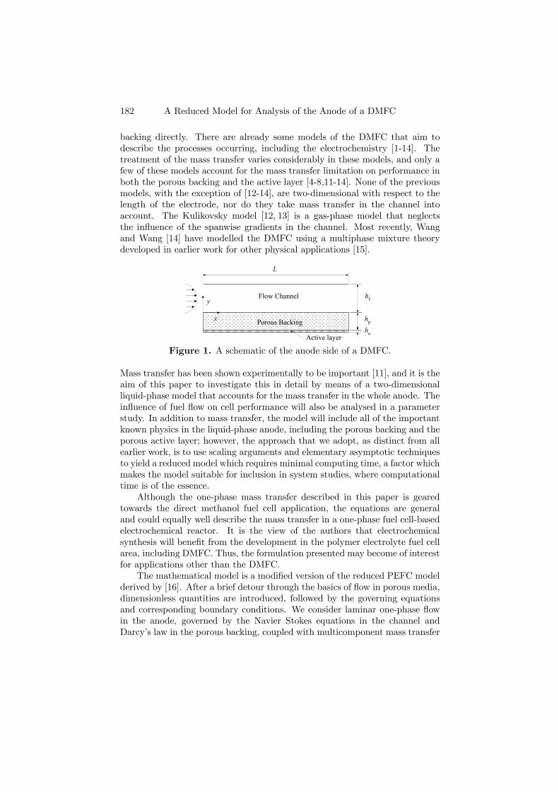
182 A Reduced Model for Analysis of the Anode of a DMFC
backing directly. There are already some models of the DMFC that aim todescribe the processes occurring, including the electrochemistry [1-14]. Thetreatment of the mass transfer varies considerably in these models, and only afew of these models account for the mass transfer limitation on performance inboth the porous backing and the active layer [4-8,11-14]. None of the previousmodels, with the exception of [12-14], are two-dimensional with respect to thelength of the electrode, nor do they take mass transfer in the channel intoaccount. The Kulikovsky model [12, 13] is a gas-phase model that neglectsthe influence of the spanwise gradients in the channel. Most recently, Wangand Wang [14] have modelled the DMFC using a multiphase mixture theorydeveloped in earlier work for other physical applications [15].
hf
hp
L
y
x
Flow Channel
Porous Backing
Active layerha
Figure 1. A schematic of the anode side of a DMFC.
Mass transfer has been shown experimentally to be important [11], and it is theaim of this paper to investigate this in detail by means of a two-dimensionalliquid-phase model that accounts for the mass transfer in the whole anode. Theinfluence of fuel flow on cell performance will also be analysed in a parameterstudy. In addition to mass transfer, the model will include all of the importantknown physics in the liquid-phase anode, including the porous backing and theporous active layer; however, the approach that we adopt, as distinct from allearlier work, is to use scaling arguments and elementary asymptotic techniquesto yield a reduced model which requires minimal computing time, a factor whichmakes the model suitable for inclusion in system studies, where computationaltime is of the essence.
Although the one-phase mass transfer described in this paper is gearedtowards the direct methanol fuel cell application, the equations are generaland could equally well describe the mass transfer in a one-phase fuel cell-basedelectrochemical reactor. It is the view of the authors that electrochemicalsynthesis will benefit from the development in the polymer electrolyte fuel cellarea, including DMFC. Thus, the formulation presented may become of interestfor applications other than the DMFC.
The mathematical model is a modified version of the reduced PEFC modelderived by [16]. After a brief detour through the basics of flow in porous media,dimensionless quantities are introduced, followed by the governing equationsand corresponding boundary conditions. We consider laminar one-phase flowin the anode, governed by the Navier Stokes equations in the channel andDarcy’s law in the porous backing, coupled with multicomponent mass transfer
E. Birgersson et al. 183
equations for methanol and carbon dioxide. The flow can be treated as a dilutemixture. In a previous paper [11], the pore diffusion, finite ionic conductivityand the complex methanol oxidation kinetics of the anode electrode were alltaken into account. In the present paper, we use that model to derive anexpression that can be used to reduce the governing equations in the active layerto a boundary condition for the flow in the rest of geometry; as a consequence,the present model implicitly accounts for the porous effects and the reactionkinetics of the previous study. The modeled electrode is 23 µm thick and iscomprised of 0.8 mg/cm2 of PtRu (1:1, 40% on carbon) and 1.7 mg/cm2 of
NafionR°. The model, as all previous DMFC models [1-14], is isothermal. For
very low fuel flow rates, this is not a particularly good assumption, althoughit becomes so if the cell is tempered. Since the kinetic equations used werederived at 70oC, all physical properties are also taken at that temperature.Adaption of the reduced model to the anode shows the conditions for whichthe the velocity field in the channel decouples from the rest of the flow and canbe solved a priori. The operating conditions at the anode enable a reduction ofthe mass transfer equations to just one scalar transport equation for methanolin the flow channel; the solutions in the active layer and porous backing are thengiven by elementary analytical expressions involving a function that requiresthe numerical solution of a simple transcendental equation. The reduced model,solved numerically with a Modified Box discretization scheme, is verified againsttwo commercial codes which solve for the full set of governing equations andboundary conditions. The results from a parameter study of the anode arediscussed and conclusions are drawn.
2. Mathematical formulation
A reduced model for tricomponent flow in the slender cathode of a polymerelectrolyte fuel cell (PEFC) has been derived recently by [16]. This reducedmodel is based on a rigorous mathematical reduction of the full elliptic gov-erning equations for two-dimensional one-phase conservation of mass, speciesand momentum in the flow channel and adjacent porous backing. Further-more, that model is general enough to be adaptable, after minor modifications,to the anode of the DMFC. To limit the algebra, however, we will here giveonly the modified equations as they pertain to the anode once the slendernessof the geometry has been invoked, and refer to [16] for the full derivation ofthese. The dimensional equations are shown in Appendix A, together with thedimensional boundary conditions in Appendix B.
In the channel, see Figure 1, conservation of momentum is given by theNavier Stokes equation for an incompressible fluid and in the porous backingby Darcy’s law. Continuity of mass and species transport equations are solvedfor the liquid mixture, containing methanol, water and carbon dioxide.
These are nondimensionalised with the parameters given below. Recogniz-ing the slenderness of the geometry, i.e. that the ratio of the heights of theflow channel, porous backing and active layer to the length is much smaller

184 A Reduced Model for Analysis of the Anode of a DMFC
than one, hf/L << 1, hp/L << 1, ha/L << 1, we rescale once more to obtainwhat is called the narrow-gap approximation. Mathematically, this additionalscaling essentially entails the reduction of elliptic PDEs to parabolic PDEs inthe flow channel and ODEs in the porous backing. The resulting equations areoutlined below.
2.1. Basics of flow in porous media. A proper description of the trans-port processes in a porous medium requires the introduction of volume-averagedequations and associated intrinsic and superficial properties, and we introducethese details first; see e.g. [17-19] for more details on volume averaging.
We let hφi and hφi(l) denote superficial and intrinsic properties, defined as
hφi ≡ 1
V
ZVφdV 0, (2)
and
hφi(l) ≡ 1
V(l)ZVφdV 0, (3)
where V is the total volume of the Representative Elementary Volume (REV)and V(l) is the volume of the void in the REV. Introducing the porosity, γ =V(l)/V, the two averages are related through
hφi = γ hφi(l) . (4)
2.2. Dimensionless quantities. The model is based on the followingnondimensionalization:
ey = y
L, ex = x
L, ep = p− pout
ρ (U in)2 , hepi(l) = hpi(l) − pout
ρ (U in)2 , Mi =
Mi
[M ],
hIi = hii[i]
, eD =D
[D],DeDE(l) = hDi(l)
[D], ev = v
U in, hevi = hvi
U in.
Here, p is the pressure (with pout as the outlet pressure), Mi is the molecularmass of species i with typical scale [M ], D and hDi(l) are the diffusion tensorsin the channel and porous backing with characteristic scale [D], i is the currentdensity with scale [i], L is the length of the channel, U in is the maximumvelocity for a fully developed laminar velocity profile at the inlet, v = (u, v)is the velocity in the channel, hvi = (hui , hvi) is the superficial velocity in theporous backing. In what follows we will take the density to be constant andequal to that of water; this is justified on physical grounds at the start of thesubsection on “Constitutive relations”. The dimensionless parameters whichappear are
Re ≡ ρU inL
µ, Sc ≡ µ
[D]ρ, Da ≡ κp
L2, Λ ≡ [i][M ]
ρU inF,
where Re, Sc and Da are the Reynolds, Schmidt and Darcy numbers, respec-tively, and Λ describes the ratio of the mass flux of the electrochemical reactionto the convective mass flux, whence it can be viewed as a Damköhler number.

E. Birgersson et al. 185
Here, κp is the permeability of the porous backing, µ is the dynamic viscosityand F is Faraday’s constant.
Since the typical anode is slender, i.e. hp/L, hf/L << 1, we scale furtherwith
X = ex, Y =eyσ, U = eu, V =
evσ,
where σ ≡ hf/L and hp is the height of the porous backing. We will later alsouse the notation H for the ratio hp/hf .
We neglect terms of O(σ) or lower, although combinations of σ and otherdimensionless properties are retained, and introduce the additional dimension-less numbers
∆ ≡ 1
Reσ2, Ω ≡ Λ
σ, Σ ≡ σ2
Da12
;
here, ∆ is the reciprocal of the reduced Reynolds number and Ω is the modifiedDamköhler number.
2.3. Governing equations. With the simplifications outlined above, thedimensionless form of the dimensional equations given in Appendix A is, forthe channel,
∂U
∂X+
∂V
∂Y= 0, (5)
U∂U
∂X+ V
∂U
∂Y= − ∂P
∂X+∆
∂2U
∂Y 2, (6)
∂P
∂Y= 0, (7)µ
U∂
∂X+ V
∂
∂Y
¶µwMeOHwCO2
¶=∆
Sc
∂
∂Y
·eD ∂
∂Y
µwMeOHwCO2
¶¸, (8)
where wMeOH and wCO2 are the mass fractions of methanol and carbon dioxide,respectively. The species transport equation, Eq. 8, is written in a compactform, to be read as two equations, one for methanol and the other for carbondioxide, which are coupled through the diffusion tensor, eD.
The equations to be solved in the porous backing are
∂ hUi∂X
+∂ hV i∂Y
= 0, (9)
hUi = 0, (10)
∂ hP i(l)
∂Y= −∆Σ2 hV i , (11)µ
hUi ∂
∂X+ hV i ∂
∂Y
¶ÃhwMeOHi(l)
hwCO2i(l)
!=∆
Sc
∂
∂Y
"γDeDE(l) ∂
∂Y
ÃhwMeOHi(l)
hwCO2i(l)
!#.
(12)We point out that the details of the derivation of Eqs. 9-11 from Eqs. A.4and A.5 can be found in [16]. Briefly, these equations require a permeabilityκp . 10−10 m2, so that the shear-stress-induced velocity in the streamwise

186 A Reduced Model for Analysis of the Anode of a DMFC
direction at the interface between the porous backing and the flow channelis negligible, and hence can be set to zero at leading order, Eq. 10; typicalpermeabilities for the porous backing found in literature range from 10−11
m2 [14] to 10−14 m2 [12].
2.4. Boundary conditions. The full boundary conditions are given inAppendix B, and here we give only those that are needed for our reducedmodel. In particular, this means that the boundary conditions at the outlet ofthe channel and at the right-hand end of the porous backing are redundant,and we therefore do not include them here.
At the inlet (X = 0, 0 ≤ Y ≤ 1), we specify
U = 4¡Y − Y 2
¢, (13)
which corresponds to fully developed laminar flow, andµwMeOHwCO2
¶=
µwinMeOHwinCO2
¶. (14)
At the upper wall in the channel (0 ≤ X ≤ 1, Y = 1), there is no slip andno normal flow, so that
U = V = 0, (15)
and no componental flux, so that
∂wMeOH∂Y
=∂wCO2
∂Y= 0. (16)
At the left wall of the porous backing, (X = 0, −H ≤ Y ≤ 0), we prescribeno normal flow and no componental flux, so that
hUi = ∂ hwMeOHi(l)
∂X=
∂ hwCO2i(l)
∂X= 0. (17)
At the channel/porous backing interface (0 ≤ X ≤ 1, Y = 0), the reducedmodel requires continuity of streamwise and normal velocity components:
U = hUi , (18)
V = hV i . (19)
For the species, continuity of mass fractions and fluxes are prescribedµwMeOHwCO2
¶=
ÃhwMeOHi(l)
hwCO2i(l)
!, (20)
eD ∂
∂Y
µwMeOHwCO2
¶= γ
DeDE(l) ∂
∂Y
ÃhwMeOHi(l)
hwCO2i(l)
!. (21)
At the interface between the porous backing and the active layer (0 ≤ X ≤1, Y = −H), we specify
hV i = −Ω hIiΦ6
, (22)
E. Birgersson et al. 187
hV iÃhwMeOHi(l)
hwCO2i(l)
!− ∆Sc
γDeDE(l) ∂
∂Y
ÃhwMeOHi(l)
hwCO2i(l)
!
=Ω hIi6
µ−MMeOH
MCO2
¶, (23)
where Φ ≡ ((1 + 6αH2O)MH2O +MMeOH −MCO2) ; in the latter, αH2O is thenumber of water molecules dragged through the membrane with each protonvia electro-osmosis. The electro-osmosis of methanol is neglected as it is con-siderably lower than the electro-osmosis of water [6]. Scott et al. [6] assumethat αMeOH ≈ xMeOH αH2O. For the cases considered, the highest value of themolar fraction of methanol is 0.019, whence the influence of the electro-osmosisof methanol is neglected. In the boundary condition for methanol we have ne-glected the diffusion of methanol through the membrane, which is a reasonableassumption for most practical DMFC applications since a high diffusion flowwould lead to considerable loss of fuel and an unfavourable mixed potential atthe cathode [22]. If the methanol crossover is substantial, then a correspondingterm could easily be added to Eq. 23, see e.g. [6] for a detailed discussion onmethanol crossover. These boundary conditions can be derived from Faraday’slaw and the theory of multicomponent mixtures, and have been used in dimen-sional form for PEFC models by [16,20,21]. The novel feature in this paper isto combine these boundary conditions with an expression for the local superfi-cial current density, which still takes concentration and potential gradients inthe active layer into account, yet does not require a spatial resolution of theactive layer in the model.
2.5. Constitutive relations. By extrapolating literature data to 70oC,the influence of methanol on the density is estimated to lower the density by0.4% at 2 wt.% methanol in the mixture [23]. This contribution can safely beneglected, whence we take the density of the mixture, ρ, as that of pure water.
The diffusion tensor in the channel can be simplified to a diagonal tensor,since the system can be treated as a dilute solution, rendering the cross termsredundant, i.e
D =
·DMeOH,H2O 0
0 DCO2,H2O
¸; (24)
in the porous backing, a Bruggeman relationship for the superficial total massdiffusion tensor, in the form
hDi = γ32D, (25)
will be used. Note that we specify the superficial diffusion tensor here and notthe intrinsic.
In order to take the porous effects of the actual active layer into account, aprevious model [11] is used to generate an expression for the local current den-sity, that can be used for the boundary conditions at the active layer/porousbacking. This current density implicitly accounts for the same effects as wereconsidered in that paper, i.e. pore diffusion in the active layer, finite ionic con-ductivity and the complex methanol oxidation kinetics. Appendix C outlines

188 A Reduced Model for Analysis of the Anode of a DMFC
how the model in the previous paper is reduced, in dimensional form, to
hii = A³hcMeOHi(l)
´B exp¡αAFRT (EA −E0)
¢1 + exp
¡αAFRT (EA −E0)
¢ , (26)
where hii is the local superficial current density, EA is the anode potential mea-sured at the active layer/membrane interface versus a DHE reference electrode(EA = 0.33 − 0.40 V [11]), αA is the Tafel slope measured at low potentials,hcMeOHi(l) = hρi(l) hwMeOHi(l) /MMeOH is the methanol concentration at theporous backing/active layer interface, and A, B and E0 are three experimen-tally fitted parameters (see Table I).
The vapor pressure of the dissolved carbon dioxide is taken from Henry’slaw for molar fractions, assuming that the low fraction of methanol in the liquidwater does not influence the Henry’s law coefficient, HCO2 :
pCO2= xCO2
HCO2. (27)
2.6. Magnitude of dimensionless numbers. To determine the magni-tude of the dimensionless numbers, we need typical scales for the anode, whichare given by [M ] ∼ 10−2 kg mol−1, [i] ∼ 4× 10³ Am−2 and [D] ∼ 10−9 m2s−1;the remaining parameters are summarized in Table I.The dimensionless numbers are thence Re ∼ 103, Sc ∼ 50, Da ∼ 10−10, Λ ∼4 × 10⁻⁴, σ ∼ 10−2, Ω ∼ 4 × 10⁻², ∆ ∼ 10 and Σ ∼ 10. Noting the ordersof magnitude of these various parameters enables us to simplify the modelequations further, as follows.
Table I. Base-case parameters.Parameter Value UnitsA 1.57× 10² [-]αA 7.9× 10⁻¹ [-]αH2O 2.5, see Ref. [3] [-]αMeOH αMeOH ≈ xMeOH αH2O [6] [-]B 6.10×10⁻¹ [-]DMeOH,H2O 6.69× 10⁻⁹ m2s−1
E0 5.04×10⁻¹ VEA 0.5 VF 96487 As mol−1
γ 8.75× 10⁻¹ [-]ha 2.3× 10⁻⁵, see Ref. [11] mhf 10−3 mhp 1.8× 10⁻⁴ mHCO2 3903, see Ref. [24] barκp 10−12 m2
L 1× 10⁻¹ m
E. Birgersson et al. 189
MCO2 4.4× 10⁻² kg mol−1
MH2O 1.8× 10⁻² kg mol−1
MMeOH 3.2× 10⁻² kg mol−1
µ 4.1× 10⁻⁴ kgm−1s−1
pout 101.325× 10³ PaR 8.314 Jmol−1K−1
ρ 978 kg m−3
T 343 KU in 3
2 × 3× 10−3 ms−1
winCO20 [-]
winMeOH 3.2× 10⁻² [-]
2.7. Adaption to the anode of a DMFC. We note that wH2O >>wMeOH and wH2O >> wCO2 , so writing
wMeOH + wCO2 = 1− winH2O, (28)
we only need to solve the mass transfer equation for methanol and this relation-ship will provide the mass fraction of carbon dioxide. This also simplifies thediffusion coefficient DMeOH,H2O, which we can treat as constant for the dilutesystem; thus, an appropriate choice for the characteristic diffusion coefficientscale, [D], is [D] = DMeOH,H2O.
Returning to the porous backing and the velocity boundary condition, Eq.22, we scale the spanwise velocity in the porous backing further according toDbV E = hV i
Ω. (29)
Using Eq. 10 to eliminate hUi in Eqs. 9 and 12, Eqs. 9, 11 and 12 become,respectively,
∂DbV E∂Y
= 0, (30)
∂ hP i(l)
∂Y= −∆Σ2Ω
DbV E , (31)
ΩDbV E ∂ hwMeOHi(l)
∂Y=∆
Scγ32∂2 hwMeOHi(l)
∂Y 2. (32)
The normal velocity in the channel is bounded by Eqs. 15 and 19, whencewe scale it with Ω. The governing equations, Eqs. 5-8 in the channel are thengiven by

190 A Reduced Model for Analysis of the Anode of a DMFC
∂U
∂X+Ω
∂ bV∂Y
= 0, (33)
U∂U
∂X+ΩbV ∂U
∂Y= − ∂P
∂X+∆
∂2U
∂Y 2, (34)
∂P
∂Y= 0, (35)µ
U∂
∂X+ΩbV ∂
∂Y
¶µwMeOHwCO2
¶=
∆
Sc
∂
∂Y
·eD ∂
∂Y
µwMeOHwCO2
¶¸. (36)
Now, since Ω ∼ O¡10−2
¢¿ 1, we can safely neglect terms of O(Ω), which
corresponds to V = 0; furthermore, Eqs. 10 and 18 imply that U = 0 at Y = 0.Consequently, we find that the inlet condition for a fully developed laminarvelocity profile satisfies the momentum equation downstream, and thence that,at leading order, the velocity decouples from the mass transfer in the channel;all that remains to be solved there is
4¡Y − Y 2
¢ ∂wMeOH∂X
=∆
Sc
∂2wMeOH∂Y 2
. (37)
Now, Eqs. 22 and 30 combine to give, for the entire porous backing,DbV E = −hIiΦ6
;
then, since the current density is a function of X alone, we haveDbV E =DbV (X)E. We can integrate Eq. 32 and, using Eq. 22 and 23, we arrive
at
−Ω hIiΦ6
hwMeOHi(l) −∆
Scγ32∂ hwMeOHi(l)
∂Y= −Ω hIi
6MMeOH. (38)
Furthermore, choosing [M ] =MMeOH, whenceMMeOH = 1, Eq. 38 becomes
Φ hwMeOHi(l) +6∆
ScΩ hIiγ32∂ hwMeOHi(l)
∂Y= 1. (39)
Returning to the expression for the current density, Eq. 40, and choosing the,as yet, unspecified current density scale, [i], to be
[i] = A
µρwinMeOHMMeOH
¶Bexp
¡αAFRT (EA −E0)
¢1 + exp
¡αAFRT (EA −E0)
¢ , (40)
we obtain
hIi =³hwMeOHi(l) (X,−H)/winMeOH
´B. (41)
Integrating Eq. 39 gives
hwMeOHi(l) (X,Y ) =1
Φ+ C exp
µ−ΦScΩ hIi
6∆γ32
Y
¶, (42)
E. Birgersson et al. 191
where C is an integration constant to be determined shortly. At Y = −H, wehave
hwMeOHi(l) (X,−H) = 1
Φ+ C exp
µΦScΩ hIi6∆γ
32
H¶, (43)
and at Y = 0,
hwMeOHi(l) (X, 0) =1
Φ+ C, (44)
whence the integration constant C is given by the methanol mass fraction at theinterface between the porous backing and the channel. Recalling the boundaryconditions for the plain/porous interface, Eqs. 20 and 21, for the methanoltransport equation, we combine these two to obtain just one boundary conditionfor the channel at Y = 0 :
∂wMeOH(X, 0)
∂Y+ΦScΩ hIi6∆
µwMeOH(X, 0)− 1
Φ
¶= 0. (45)
This is valid for any profile hIi , which is a function of the value of hwMeOHi(l)at Y = −H; for the profile considered in this paper, hIi can be determined interms of wMeOH(X, 0) through the transcendental equation
winMeOH hIi1B =
1
Φ+
µwMeOH(X, 0)− 1
Φ
¶exp
µΓ hIi6
¶, (46)
where Γ = ΦScΩH/(∆γ 32 ).
In summary, the adaption of the reduced model to the anode of a DMFCis based on the fact that the anode operates at a large water fraction and thatthe magnitude of the dimensionless parameter Ω is much smaller than 1; indimensionless form, the latter condition is
[i] [M ]L
ρU inFhf¿ 1.
Mathematically, we find that these reductions enable us to obtain solutionsfor the porous backing in simple analytical form; for the channel, we havean analytical solution for the velocity field and a linear diffusion equation forthe methanol concentration, although subject to a highly non-linear boundarycondition at the interface with the porous backing.
3. Numerics and verification
We have to resort to a numerical scheme to solve the transport equationfor methanol in the channel, since no further simplifications are possible. Thisentails solving Eq. 37, subject to the boundary conditions Eqs. 16 and 45 andthe inlet condition for methanol, Eq. 14.
The governing equations are parabolic, for which a Modified Box discretiza-tion scheme is suitable [25]. The scheme leads to a block tridiagonal matrix,allowing fast computations. The resulting system of non-linear equations issolved with a Newton-Raphson-based algorithm in MATLAB 6.
To confirm the validity of the reduced model, its predictions were comparedwith numerical results obtained using two other softwares, wherein the full

192 A Reduced Model for Analysis of the Anode of a DMFC
elliptic governing equations and boundary conditions are implemented. Oneis FEMLAB 2.2 (see [26] for details), a commercial finite element solver fora wide variety of engineering applications; the other is CFX-4.4 (see [27] fordetails), a commercial CFD software which uses finite volumes. Comparison,shown in Figure 2, was carried out in terms of the local superficial currentdensity obtained along the anode for a variety of values for the nondimensionalparameters ∆ and Ω (given in Table II).
Table II. Values of ∆ and Ω used for the verification.∆ 0.932 2.79 9.32 27.9 93.2 279Ω 3.76×10⁻³ 1.13×10⁻² 3.76×10⁻² 1.13×10⁻¹ 3.76×10⁻¹ 1.13
These were obtained by varying the inlet velocity, U in, and keeping all otherphysical parameters constant; in particular, the base case corresponds to ∆ =9.32 and Ω = 3.76× 10⁻².
0 0.1 0.2 0.3 0.4 0.5 0.6 0.7 0.8 0.9 10
500
1000
1500
2000
2500
3000
3500
4000
4500
X
<i>
/Am
-2
∆, Ω increasing
Figure 2. Verification of the reduced model. (· · ·) corresponds to theCFX-4.4 solution with 104 number of nodes, (–) is the Femlab solution for∼1000 adapted nodes and markers are for the reduced model, with 104 cells.(F): ∆ = 0.932, (o): ∆ = 2.79, (×): ∆ = 9.32, (+): ∆ = 27.9, (¤): ∆ = 93.2,(O): ∆ = 279.
Several features are apparent. First, for the higher (∆,Ω)-combinations,the reduced model starts to deviate from the full solution, since the spanwisevelocity due to the electrochemical reaction now is of the same order of mag-nitude as the streamwise inlet velocity, i.e. Ω is no longer much smaller thanunity and the spanwise velocity in the channel is no longer negligible. Never-theless, the local current densities from the reduced model remain close to the
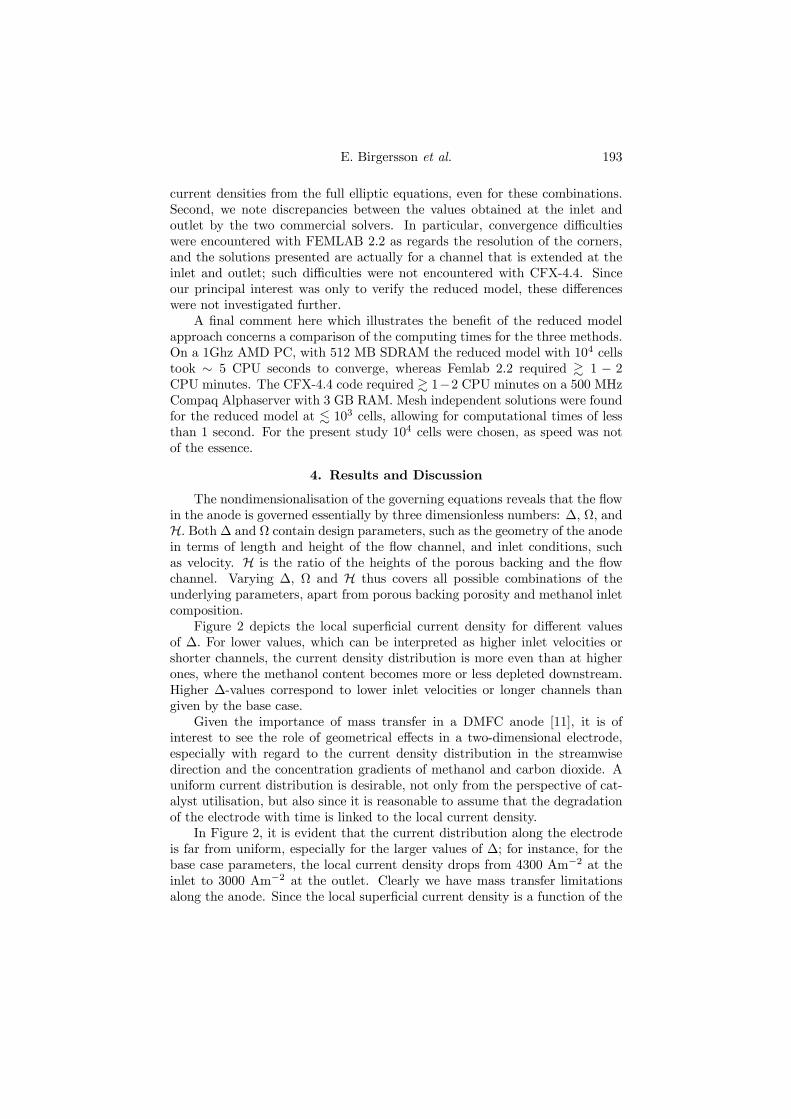
E. Birgersson et al. 193
current densities from the full elliptic equations, even for these combinations.Second, we note discrepancies between the values obtained at the inlet andoutlet by the two commercial solvers. In particular, convergence difficultieswere encountered with FEMLAB 2.2 as regards the resolution of the corners,and the solutions presented are actually for a channel that is extended at theinlet and outlet; such difficulties were not encountered with CFX-4.4. Sinceour principal interest was only to verify the reduced model, these differenceswere not investigated further.
A final comment here which illustrates the benefit of the reduced modelapproach concerns a comparison of the computing times for the three methods.On a 1Ghz AMD PC, with 512 MB SDRAM the reduced model with 104 cellstook ∼ 5 CPU seconds to converge, whereas Femlab 2.2 required & 1 − 2CPU minutes. The CFX-4.4 code required & 1−2 CPU minutes on a 500 MHzCompaq Alphaserver with 3 GB RAM. Mesh independent solutions were foundfor the reduced model at . 103 cells, allowing for computational times of lessthan 1 second. For the present study 104 cells were chosen, as speed was notof the essence.
4. Results and Discussion
The nondimensionalisation of the governing equations reveals that the flowin the anode is governed essentially by three dimensionless numbers: ∆, Ω, andH. Both ∆ and Ω contain design parameters, such as the geometry of the anodein terms of length and height of the flow channel, and inlet conditions, suchas velocity. H is the ratio of the heights of the porous backing and the flowchannel. Varying ∆, Ω and H thus covers all possible combinations of theunderlying parameters, apart from porous backing porosity and methanol inletcomposition.
Figure 2 depicts the local superficial current density for different valuesof ∆. For lower values, which can be interpreted as higher inlet velocities orshorter channels, the current density distribution is more even than at higherones, where the methanol content becomes more or less depleted downstream.Higher ∆-values correspond to lower inlet velocities or longer channels thangiven by the base case.
Given the importance of mass transfer in a DMFC anode [11], it is ofinterest to see the role of geometrical effects in a two-dimensional electrode,especially with regard to the current density distribution in the streamwisedirection and the concentration gradients of methanol and carbon dioxide. Auniform current distribution is desirable, not only from the perspective of cat-alyst utilisation, but also since it is reasonable to assume that the degradationof the electrode with time is linked to the local current density.
In Figure 2, it is evident that the current distribution along the electrodeis far from uniform, especially for the larger values of ∆; for instance, for thebase case parameters, the local current density drops from 4300 Am−2 at theinlet to 3000 Am−2 at the outlet. Clearly we have mass transfer limitationsalong the anode. Since the local superficial current density is a function of the
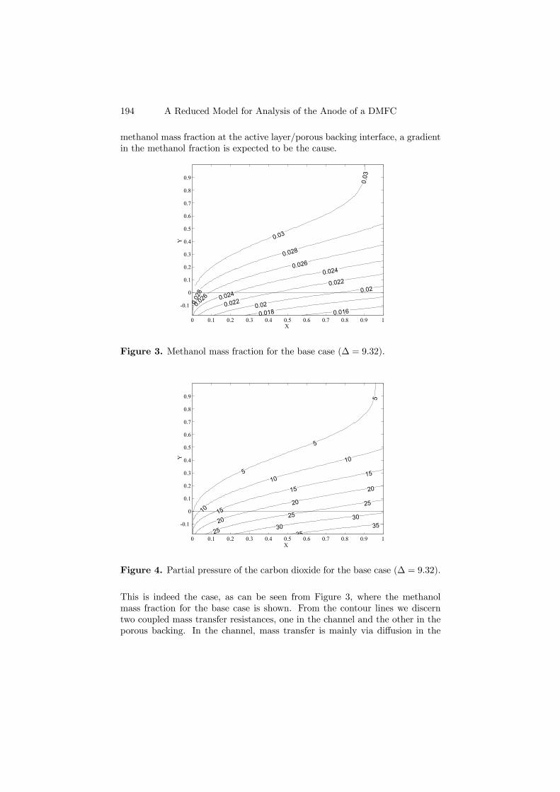
194 A Reduced Model for Analysis of the Anode of a DMFC
methanol mass fraction at the active layer/porous backing interface, a gradientin the methanol fraction is expected to be the cause.
0 0.1 0.2 0.3 0.4 0.5 0.6 0.7 0.8 0.9 1
-0.1
0
0.1
0.2
0.3
0.4
0.5
0.6
0.7
0.8
0.9
X
Y 0.03
0.03
0.02
8
0.028
0.026
0.026
0.024
0.024
0.022
0.022
0.02
0.02
0.018 0.016
Figure 3. Methanol mass fraction for the base case (∆ = 9.32).
0 0.1 0.2 0.3 0.4 0.5 0.6 0.7 0.8 0.9 1
-0.1
0
0.1
0.2
0.3
0.4
0.5
0.6
0.7
0.8
0.9
X
Y
5
5
5
10
10
10
15
15
15
20
20
20
25
25
25
3030
3535
Figure 4. Partial pressure of the carbon dioxide for the base case (∆ = 9.32).
This is indeed the case, as can be seen from Figure 3, where the methanolmass fraction for the base case is shown. From the contour lines we discerntwo coupled mass transfer resistances, one in the channel and the other in theporous backing. In the channel, mass transfer is mainly via diffusion in the
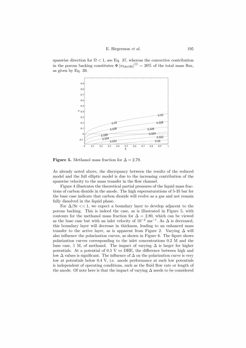
E. Birgersson et al. 195
spanwise direction for Ω < 1, see Eq. 37, whereas the convective contributionin the porous backing constitutes Φ hwMeOHi(l) ∼ 20% of the total mass flux,as given by Eq. 39.
0 0.1 0.2 0.3 0.4 0.5 0.6 0.7 0.8 0.9 1
-0.1
0
0.1
0.2
0.3
0.4
0.5
0.6
0.7
0.8
0.9
X
Y
0.03
0.03
0.028
0.028
0.026
0.026
0.0240.024
0.0220.022
0.02
Figure 5. Methanol mass fraction for ∆ = 2.79.
As already noted above, the discrepancy between the results of the reducedmodel and the full elliptic model is due to the increasing contribution of thespanwise velocity to the mass transfer in the flow channel.
Figure 4 illustrates the theoretical partial pressures of the liquid mass frac-tions of carbon dioxide in the anode. The high supersaturations of 5-35 bar forthe base case indicate that carbon dioxide will evolve as a gas and not remainfully dissolved in the liquid phase.
For ∆/Sc << 1, we expect a boundary layer to develop adjacent to theporous backing. This is indeed the case, as is illustrated in Figure 5, withcontours for the methanol mass fraction for ∆ = 2.80, which can be viewedas the base case but with an inlet velocity of 10−2 ms−1. As ∆ is decreased,this boundary layer will decrease in thickness, leading to an enhanced masstransfer to the active layer, as is apparent from Figure 2. Varying ∆ willalso influence the polarization curves, as shown in Figure 6. The figure showspolarization curves corresponding to the inlet concentrations 0.2 M and thebase case, 1 M, of methanol. The impact of varying ∆ is larger for higherpotentials. At a potential of 0.5 V vs DHE, the difference between high andlow ∆ values is significant. The influence of ∆ on the polarization curve is verylow at potentials below 0.4 V, i.e. anode performance at such low potentialsis independent of operating conditions, such as the fluid flow rate or length ofthe anode. Of note here is that the impact of varying ∆ needs to be considered

196 A Reduced Model for Analysis of the Anode of a DMFC
above a certain potential rather than above a certain current density, contraryto what one might at first expect.
0 500 1000 1500 2000 2500 3000 3500 4000 45000.3
0.32
0.34
0.36
0.38
0.4
0.42
0.44
0.46
0.48
0.5E A
/V
vs D
HE
<i>av /Am-2
∆ increasinga) b) ∆ increasing
Figure 6. Polarization curves for ∆ = 0.279, 0.932, 2.79, 9.32 and 27.9: a)winMeOH = 6.4× 10⁻³ (0.2 M) and b) winMeOH = 3.2× 10⁻² (1 M).
0 0.1 0.2 0.3 0.4 0.5 0.6 0.7 0.8 0.9 12500
3000
3500
4000
4500
5000
X
<i>
/A
m-2 h
p/h
f increasing
Figure 7. Local current density for different H = hp/hf . H = 0, 6.75× 10−2,1.35× 10−1, 2.03× 10⁻¹ and 2.70× 10⁻¹. Keeping the height of the flowchannel fixed at hf =10−3 m, these curves would correspond to hp = 0 m,6.75× 10−5 m, 1.35× 10⁻⁴ m, 2.03× 10⁻⁴ m and 2.70× 10⁻⁴ m.

E. Birgersson et al. 197
It is interesting to see the model prediction when the height of the porousbacking or the flow channels is changed. From Figure 7, where we have keptthe base case parameters and varied H, it is clear that it would be desirableto have smaller H values. This corresponds to a thin porous backing and/orbroad flow channels. The performance in terms of total current density at agiven anode potential can potentially be improved by ∼10% for the base caseset of parameters, by letting H → 0. The figure also shows that the shape ofthe local current density distribution is almost entirely unaffected by changingH.
0 5 10 15 20 250
10
20
30
40
50
60
70
80
∆
Pmax
CO
2 /b
ar a.)
b.)
c.)
2 4 60
1
2
3
4
5
∆
Pmax
CO
2 /b
ar
b)
c)
Figure 8. The maximum pressure in the porous backing (–) and theadjacent channel (· · ·) for different ∆: a) EA = 0.5 V, b) EA = 0.40 V and c)EA = 0.35 V.
An important question arises when the carbon dioxide partial pressureis as high as in the base case: can the pressure be reduced by lowering ∆?Figure 8 gives the maximum partial pressure of carbon dioxide in the twodifferent media, the porous backing and the flow channel. It is obvious fromthe figure that even for very low values of ∆, thermodynamics imply that thecarbon dioxide from the electrochemical reaction will evolve as a gas, unless thepotential is very low. The conditions for one-phase flow are thus satisfied onlyfor ∆ << 1 in conjunction with low potentials, typically EA . 0.35 V. Previouscalculations [28] indicate that carbon dioxide gas will form in the gas diffusionlayer, or even in the porous electrode, at base-case supersaturations. Sincenot even very large flows of fuel (lower values of ∆) prevent the formation ofcarbon dioxide gas at moderate current densities, it is inevitable that a modelthat aims to capture the full physics in a DMFC has to take two-phase flowinto account.
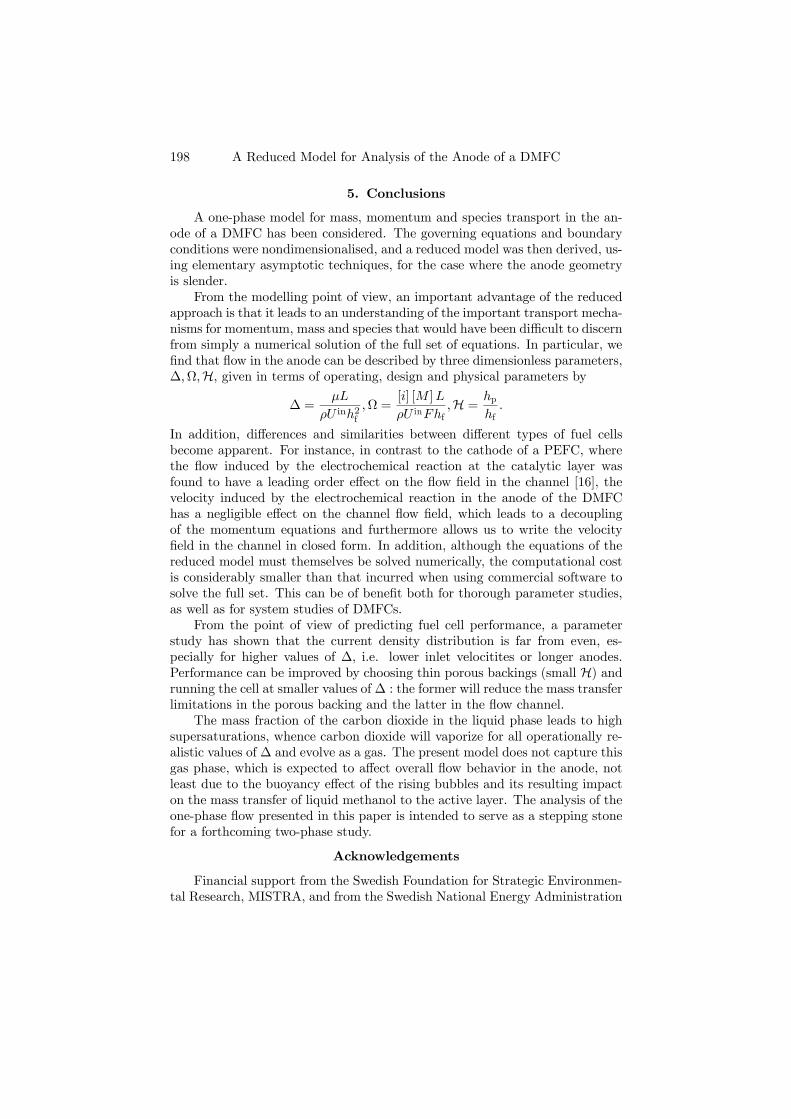
198 A Reduced Model for Analysis of the Anode of a DMFC
5. Conclusions
A one-phase model for mass, momentum and species transport in the an-ode of a DMFC has been considered. The governing equations and boundaryconditions were nondimensionalised, and a reduced model was then derived, us-ing elementary asymptotic techniques, for the case where the anode geometryis slender.
From the modelling point of view, an important advantage of the reducedapproach is that it leads to an understanding of the important transport mecha-nisms for momentum, mass and species that would have been difficult to discernfrom simply a numerical solution of the full set of equations. In particular, wefind that flow in the anode can be described by three dimensionless parameters,∆,Ω,H, given in terms of operating, design and physical parameters by
∆ =µL
ρU inh2f,Ω =
[i] [M ]L
ρU inFhf,H =
hphf
.
In addition, differences and similarities between different types of fuel cellsbecome apparent. For instance, in contrast to the cathode of a PEFC, wherethe flow induced by the electrochemical reaction at the catalytic layer wasfound to have a leading order effect on the flow field in the channel [16], thevelocity induced by the electrochemical reaction in the anode of the DMFChas a negligible effect on the channel flow field, which leads to a decouplingof the momentum equations and furthermore allows us to write the velocityfield in the channel in closed form. In addition, although the equations of thereduced model must themselves be solved numerically, the computational costis considerably smaller than that incurred when using commercial software tosolve the full set. This can be of benefit both for thorough parameter studies,as well as for system studies of DMFCs.
From the point of view of predicting fuel cell performance, a parameterstudy has shown that the current density distribution is far from even, es-pecially for higher values of ∆, i.e. lower inlet velocitites or longer anodes.Performance can be improved by choosing thin porous backings (small H) andrunning the cell at smaller values of ∆ : the former will reduce the mass transferlimitations in the porous backing and the latter in the flow channel.
The mass fraction of the carbon dioxide in the liquid phase leads to highsupersaturations, whence carbon dioxide will vaporize for all operationally re-alistic values of ∆ and evolve as a gas. The present model does not capture thisgas phase, which is expected to affect overall flow behavior in the anode, notleast due to the buoyancy effect of the rising bubbles and its resulting impacton the mass transfer of liquid methanol to the active layer. The analysis of theone-phase flow presented in this paper is intended to serve as a stepping stonefor a forthcoming two-phase study.
Acknowledgements
Financial support from the Swedish Foundation for Strategic Environmen-tal Research, MISTRA, and from the Swedish National Energy Administration

E. Birgersson et al. 199
is gratefully acknowledged. The work was done within the framework of theJungner Center. J. Nordlund gratefully acknowledges a scholarship from theErnst Johnson foundation. In addition, the authors wish to thank the refereesfor their comments on an earlier version of the paper.
200 A Reduced Model for Analysis of the Anode of a DMFC
Appendix A. Governing equations in dimensional form
Flow channel.- The equations for the conservation of mass and momentum,given respectively by
∇ · v = 0, (A.1)
∇ · (ρv⊗ v) = −∇p+ µ∇2v, (A.2)
are solved together with the scalar transport equations for methanol and carbondioxide:
∇ ·µv
µwMeOHwCO2
¶¶= ∇ ·
µD
·∇wMeOH∇wCO2
¸¶. (A.3)
Porous backing.- Darcy’s law with the Forchheimer and Brinkman exten-sion is assumed to govern the flow in the porous backing:
∇ · hvi = 0, (A.4)
hvi = −κpµ∇ hpi(l) + κp∇2
µhviγ
¶− F hvi , (A.5)
where F is the Forchheimer correction tensor. Scalar transport is given by
∇ ·Ãhvi
ÃhwMeOHi(l)
hwCO2i(l)
!!= ∇ ·
Ãγ hDi(l)
"∇ hwMeOHi(l)
∇ hwCO2i(l)
#!. (A.6)
E. Birgersson et al. 201
Appendix B. Boundary conditions in dimensional form
Inlet, outlet, upper wall, vertical walls.- For the flow channel, we specifyinlet velocity and liquid composition at x = 0, 0 ≤ y ≤ hf :
u = U in, v = 0, wMeOH = winMeOH, wCO2 = winCO2. (B.1)
At the upper channel wall (0 ≤ x ≤ L, y = hf ), there is no slip, no normalflow and no componental flux:
u = v =∂wMeOH
∂y=
∂wCO2
∂y= 0. (B.2)
At the outlet at x = L, 0 ≤ y ≤ hf , we set the pressure and no diffusivecomponental flux:
p = pout,∂v
∂x=
∂wMeOH∂x
=∂wCO2
∂x= 0. (B.3)
At the vertical walls of the porous electrode (x = 0, L, −hp ≤ y ≤ 0), we haveno normal flow, no tangential shear and no mass flux for the species:
hui = ∂ hvi∂x
=∂ hwMeOHi(l)
∂x=
∂ hwCO2i(l)
∂x= 0. (B.4)
Channel/porous backing interface.- At the fluid-porous interface at y = 0,0 ≤ x ≤ L, we specify continuity of the superificial mass fractions and fluxeswith their pointwise counterparts in the flow channel:
nMeOH · n = hnMeOHi · n, nCO2 · n = hnCO2i · n, (B.5)
hwMeOHi(l) = wMeOH, hwCO2i(l) = wCO2 , (B.6)
where n is the normal vector of the interface, coupled with continuity of thepointwise velocities, tangential and normal shear stresses in the flow channelwith their superficial counterparts in the porous backing:
v = hvi , u = hui , (B.7)
p− µ∂v
∂y= hpi− µ
γ
∂ hvi∂y
,∂u
∂y=1
γ
∂ hui∂y
. (B.8)
Active layer/porous backing interface.- At y = −hp, we treat the activelayer as a boundary condition, whence the total superficial mass flux is givenby
ρ hvi = − hii6F
((1 + 6αH2O)MH2O +MMeOH −MCO2) , (B.9)
and the componental fluxes by
ρ hviÃhwMeOHi(l)
hwCO2i(l)
!− ργ hDi(l) ∂
∂Y
ÃhwMeOHi(l)
hwCO2i(l)
!=hii6F
µ−MMeOH
MCO2
¶.
(B.10)

202 A Reduced Model for Analysis of the Anode of a DMFC
Appendix C. Reduction of the equations for the active layer
An earlier model of the porous anode electrode of the DMFC [11] showedthat the porous structure of the electrode is responsible for the mass transportlimitations and, at high currents, finite ionic conductivity. The kinetic equationof the anode reaction was also shown to be very complex. As concentrationsand potential in the active layer can vary considerably, it is desirable to takethese effects into account.
Since L >> ha, it is safe to assume that the concentration gradient in theelectrode is only a function of the distance across the electrode. For a givenpotential, any concentration of methanol at the porous backing/active layer in-terface corresponds to a local current density. As a consequence, it is possibleto express the local current density as a function of the concentration at thatlocation and the measured anode potential. Such a function will implicitly takeinto account the effects of the concentration and potential gradients. Since thekinetic equation of the anode reaction is very complex, an analytical solutionwill not be considered, but rather an expression that is parameter-adapted todata from the model of the active layer. Thus, the porous effects of the moredetailed model is considered in the resulting expression for the local superfi-cial current density. In order to obtain a simple expression, we restrict thedomain where the function is valid to 0.3V≤ E ≤ 0.51 V and 50 mol m−3 ≤hcMeOHi(l) ≤ 1000 mol m−3.
0
500
1000
0.30.350.40.450.50.5
1
1.5
2
2.5
3
3.5
4
c MeO
H /
mol
m-3
EA
/V vs DHE
log 10
<i/A
m-2
>
Figure A1. Comparison between the parameter-adapted kinetic function,used as local superficial current density for the boundary conditions at(0 ≤ X ≤ 1, Y = −H), and the result from the more detailed anodemodel [11].

E. Birgersson et al. 203
The concentration of methanol for the base case is ∼ 1000 mol m−3 at the inletand drops to about half of the inlet concentration. If the concentration or thepotential gradients within the electrode are of interest, it is always possible togenerate the gradients using the full electrode model [11].
Figure A1 gives the agreement between the adapted expression and thecurrent density from the detailed model by [11].
The parameter-adapted expression we use is then
hii = A³hcMeOHi(l)
´B exp¡αAFRT (EA −E0)
¢1 + exp
¡αAFRT (EA −E0)
¢ . (C.1)
Figure A1 shows that the new expression for the local current density correlateswell to the data from the electrode model in this region. The only exception iswhen the potential is high whilst the concentration is lower than 200 mol m−3.

204 A Reduced Model for Analysis of the Anode of a DMFC
List of symbols
A, B Experimentally fitted parametersC Integration constantDa ≡ κp
L2 Darcy numberDi,j Binary diffusion coefficients for a pair (i,j), m2s−1
E0 Experimentally fitted parameter, VEA Electrode potential of anode vs DHE, VF Faraday’s constant, A s mol−1
h Height, mH ≡ hp/hf Dimensionless height of porous backingHCO2 Henry’s law coefficient, bari Current density, Am−2
I Dimensionless current densityL Length of anode, mM Mean molecular mass, kg mol−1
Mi Molar mass of species i, kg mol−1
M, Mi Dimensionless molar massp Pressure, Paep, P Dimensionless pressuresR Gas constant, J mol−1 K−1
Re ≡ ρU inLµ Reynolds number
Sc ≡ µ[D]ρ Schmidt number
T Anode temperature, Ku, v, v Velocities, m s−1eu, ev, ev, U, V Dimensionless velocitiesV Volume of the representative elementary volume, m3
w Mass fractionx, y Coordinates in streamwise and spanwise direction, mex, ey,X, Y Dimensionless coordinates
E. Birgersson et al. 205
Greekα Coefficient for transport by
electro-osmosisαA Tafel slopeγ Porosity of the porous backingΓ ≡ ΦScΩH/(∆γ 3
2 ) Dimensionless number∆ ≡ 1
Reσ2 Dimensionless numberκp Permeability of the porous
backing, m2
Λ ≡ [i][M ]ρU inF Dimensionless number
µ Dynamic viscosity, kg m−1s−1
ρ Density, kg m−3
σ ≡ hfL Dimensionless number
Σ ≡ σ2
Da12
Dimensionless number
φ General tensorΦ ≡ ((1 + 6αH2O)MH2O +MMeOH −MCO2) Dimensionless numberΩ ≡ Λ
σ Dimensionless number
Subscriptsa Active layerCO2 Carbon dioxidef Flow channelH2O Wateri Species i(l) Liquid phaseMeOH Methanolp Porous backing
Superscriptsin Inlet(l) Liquid phaseout Outlet
Bibliography
[1] K. Scott, W. Taama and J. Cruickshank, J. Power Sources, 65, 159 (1997).[2] K. Scott, W. Taama and J. Cruickshank, J. Appl. Electrochem., 28, 289 (1998).[3] S. F. Baxter, V. S. Battaglia and R. E. White, J. Electrochem. Soc., 146, 437
(1999).[4] A. A. Kulikovsky, J. Divisek and A. A. Kornyshev, J. Electrochem. Soc., 147, 953
(2000).[5] H. Dohle, J. Divisek and R. Jung, J. Power Sources, 86, 469 (2000).[6] K. Scott, P. Argyropoulos and K. Sundmacher, J. Electroanal. Chem., 477, 97
(1999).[7] A. A. Kulikovsky, J. Appl. Electrochem., 30, 1005 (2000).[8] P. S. Kauranen, Acta Polytechnica Scandinavica, 237, 1 (1996).[9] K. Sundmacher, T. Schultz, S. Zhou, K. Scott, M. Ginkel and E. D. Gilles,
Chem. Eng. Sci., 56, 333 (2001).[10] S. Zhou, T. Schultz, M. Peglow and K. Sundmacher, Phys. Chem. Chem. Phys.,
3, 347 (2001).[11] J. Nordlund and G. Lindbergh, J. Electrochem. Soc., 149, A1107 (2002).[12] A. A. Kulikovsky, Electrochemistry Communications, 3, 460 (2001).[13] A. A. Kulikovsky, Electrochemistry Communications, 3, 572 (2001).[14] Z. H. Wang and C. Y. Wang, Proceedings Volume 2001-4, The Electroch. Soc., USA,
p. 286 (2001)[15] C. Y. Wang and P. Cheng, Int. J. Heat Mass Transfer, 39, 3607 (1996).[16] M. Vynnycky and E. Birgersson, SIAM J. Appl. Maths, 63, 1392 (2003)[17] M. Kaviany, Principles of Heat Transfer in Porous Media, 2nd ed., p. 15, Springer-
Verlag, New York (1995).[18] S. Whitaker, Transport in Porous Media, 1, 3 (1986).[19] J. C. Slattery, AIChe Journal, 13, 1066 (1967).[20] S. Dutta, S. Shimpalee and J. W. Van Zee, J. Appl. Electrochem., 30, 135 (2000).[21] J. S. Yi and T. Van Nguyen, J. Electrochem. Soc., 146, 38 (1999).[22] A. Heinzel and V.M. Barragán, J. Power Sources, 84, 70 (1999).[23] Landolt-Börnstein, New Series IV/1, p. 117, Springer, Germany (1977).[24] Solubility data series vol 62, IUPAC, Oxford, GB, (1996).[25] J. C. Tannehill, D. A. Anderson and R. H. Pletcher, Computational Fluid Me-
chanics and Heat Transfer, 2nd ed., p 462, Taylor & Francis, USA (1997).[26] FEMLAB 2.2, http://www.comsol.se.[27] CFX-4.4, http://www.cfx.aeat.com.[28] J. Nordlund, A. Roessler and G. Lindbergh, J. Appl. Electrochem., 32, 259 (2002).
206

Paper 6


The Design and Usage of a Visual DirectMethanol Fuel Cell
Joakim Nordlunda, Cyril Picardb, Erik Birgerssonc, Michael Vynny-ckyc, Göran Lindbergha
aDepartment of Chemical Engineering and Technology, Applied Electrochemistry,The Royal Institute of Technology, SE-100 44 Stockholm, SwedenbPresent address: LEGI, Ecole Nationale Supérieure d’Hydraulique et de Mécaniquede Grenoble, Saint Martin d’Hères, FrancecDepartment of Mechanics, FaxénLaboratoriet, The Royal Institute of Technology,SE-100 44, Stockholm, Sweden
Abstract. In order to better understand the influence of gas evolution on theperformance of the direct methanol fuel cell (DMFC) anode, a visual DMFC, compris-ing of a transparent anode and a cathode endplate with an integrated heat exchanger,and a picture analysis methodology were developed. The result was an inexpensive,but very powerful, tool for analyzing the role of two-phase flow. An important findingis that gas bubbles do not appear uniformly throughout the fluid flow matrix, butrather only at a few active sites. Another important finding is that the gas saturation(volume fraction of gas / volume fraction of liquid) increases along the streamwisedirection.
Key words: direct methanol fuel cell anode, two-phase flow, gas evolution,visualization, porous medium
1. Introduction
Direct methanol fuel cells (DMFCs) constitute a promising alternative tobatteries for a wide range of low power applications. Their major advantageover batteries is that they can be “recharged” with a new fuel cartridge or justtanked up with fuel. In addition, the DMFC has the potential to store energymore compactly, decreasing weight and volume or increasing time of usage.Compared to the more mature hydrogen fed fuel cell, the DMFC comprises asimpler system with more compact and safe fuel storage of liquid methanol.The electrochemical reactions occurring in a DMFC are:
Anode : CH3OH +H2O→ CO2 + 6H+ + 6e−, (1)
Cathode :3
2O2 + 6H
+ + 6e− → 3H2O, (2)X: CH3OH +
3
2O2 → CO2 + 2H2O. (3)
The carbon dioxide produced will, even at low current densities, exceedthe saturation limit for carbon dioxide in water and evolve as a gas [1]. In aseries of studies at University of Newcastle, the gas evolution on the anode side

210 The Design and Usage of a Visual Direct Methanol Fuel Cell
of a DMFC was investigated directly in the fuel cell using an end plate madeof transparent acrylic plastic [2-5]. In those studies, different flow fields weretested [5] and the importance of a well-designed flow field [2, 4] was emphasized.It was also shown that the mass transfer of methanol to the anode active layerwas reduced by the gas evolution [3]. Since mass transfer of methanol to theactive layer has been shown to be very important for the DMFC performance[1, 6], it is important to study the influence of gas evolution on the performanceto be able to reduce its adverse effects. There are, in principle, a number ofpossible measuring techniques that can be employed to study the influence ofthe gas evolution in the DMFC anode. Three of the most obvious are: probeinsertion, the use of seeding particles and still photography.
Probing will always only give local information, so a number of probeshave to be employed to give data along the anode. Probing is in principle aninexpensive and useful technique, but to insert a large amount of probes withthe required precision into the anode end plate is costly. There is also therisk of influencing the behaviour of the system, since the method is intrusive.Probing techniques that could be of interest in a study like this are: electricalprobes, optical probes, capacitance probes and hot film anemometry.
By introducing seeding particles to the fluid stream, the flow can be char-acterized by Laser Doppler Anemometry (LDA), Phase Doppler Anemometry(PDA), Particle Tracking Velocimetry (PTV) or Particle Image Velocimetry(PIV). Applying these methods, the velocities of both gas and liquid phasescan be measured [7, 8]. Both LDV and PIV have earlier been applied suc-cessfully in an electrolysis system with current-induced gas evolution [9]. Adrawback of these methods is that introducing seeding particles may well in-fluence the performance of the anode, since there are pores of a wide range ofsizes in the gas diffusion layer and the porous electrode itself where particlescould block mass transfer.
The third option, to study pictures from a visual cell, is a simple and costeffective method. It does lack the possibility to analyze the phase velocities.The method gives the gas saturation at every point of the anode at any giventime. Due to its simplicity, analyzing pictures from a visual cell is a goodstarting point for analyzing the influence of gas evolution on the performance ofthe anode. While the study and obtained results in the University of Newcastlestudies are valuable [2-5], the methodology to analyze the visual results canbe improved. There, the pictures were converted to digital images and thesubsequent analysis of the results was schematic, with no quantitative databeing gathered from the visual data.
In this work we take the data analysis a step further, in that a methodologyto acquire good visual data and to perform a high-quality and time effectiveanalysis is presented. In particular, we demonstrate how a visual cell, in com-bination with digital video recordings and picture analysis, can be used to givevaluable insight into two-phase flow in the anode of a DMFC.

J. Nordlund et al. 211
2. Experimental
2.1. The visual cell. Just as in [2-5], our cell has a plexi-glass endplateon the anode side where the current is drawn out to the sides. Figure 1 showsthe principle of the visual cell.
Transparent end plate
End plate with heat exchanger
Meshflowfield
Five layeredMEA
Humidified H2
Fuel saturatedwith CO2
Figure 1. The principle of the visual cell.
The potential drops due to the resistances in the spanwise direction of thestainless steel mesh and the current collector were computed and found to beless than 3 mV at 100 mA cm-2. Thanks to the low spanwise potential dropin the mesh, the results from a visual cell can be applied to a DMFC withthe same flow field length as the visual cell, regardless of the width of the flowfield. To minimize the contact resistances between the current collectors andthe stainless steel meshes, and between the mesh and the gas diffusion layer,the meshes and the current collectors were plated with a 10 µm thick layer ofgold.
Since it is of interest to study the DMFC at a variety of temperatures,the cell was designed to give an even temperature distribution by introducinga circuit for cooling/heating directly behind the cathode, as shown in Figure1. For the sake of temperature insulation and to provide an even clampingpressure on the flowfield mesh, the plexi-glass used in the cell is fairly thick(35 mm at the flowfield mesh). The flowfield mesh was a woven stainlesssteel mesh with the dimensions 1.50 mm, 40 mm, 130 mm in height, widthand length, respectively, and had gaps with dimensions 1.35x1.35 mm. Theporosity of the mesh was measured to be 0.87. The cell, mesh, MEA, gasketsand anode current collector are shown in Figure 2. Since the buoyancy of thecarbon dioxide bubbles is expected to have an impact on the performance ofthe DMFC, the visual cell was mounted on a rack, to allow for measurements atdifferent cell tilting angles. In this study, however, all experiments were carriedout in horizontal mode.
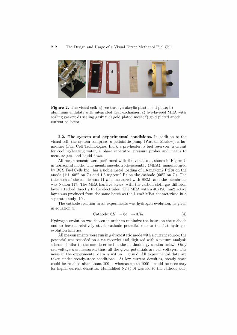
212 The Design and Usage of a Visual Direct Methanol Fuel Cell
Figure 2. The visual cell: a) see-through akrylic plastic end plate; b)aluminum endplate with integrated heat exchanger; c) five-layered MEA withsealing gasket; d) sealing gasket; e) gold plated mesh; f) gold plated anodecurrent collector.
2.2. The system and experimental conditions. In addition to thevisual cell, the system comprises a peristaltic pump (Watson Marlow), a hu-midifier (Fuel Cell Technologies, Inc.), a pre-heater, a fuel reservoir, a circuitfor cooling/heating water, a phase separator, pressure probes and means tomeasure gas- and liquid flows.
All measurements were performed with the visual cell, shown in Figure 2,in horizontal mode. The membrane-electrode-assembly (MEA), manufacturedby BCS Fuel Cells Inc., has a noble metal loading of 1.6 mg/cm2 PtRu on theanode (1:1, 60% on C) and 1.6 mg/cm2 Pt on the cathode (60% on C). Thethickness of the anode was 14 µm, measured with SEM, and the membranewas Nafion 117. The MEA has five layers, with the carbon cloth gas diffusionlayer attached directly to the electrodes. The MEA with a 40x120 mm2 activelayer was produced from the same batch as the 1 cm2 MEA characterized in aseparate study [10].
The cathode reaction in all experiments was hydrogen evolution, as givenin equation 4:
Cathode: 6H+ + 6e− → 3H2. (4)
Hydrogen evolution was chosen in order to minimize the losses on the cathodeand to have a relatively stable cathode potential due to the fast hydrogenevolution kinetics.
All measurements were run in galvanostatic mode with a current source; thepotential was recorded on a x-t recorder and digitized with a picture analysisscheme similar to the one described in the methodology section below. Onlycell voltage was measured; thus, all the given potentials are cell voltages. Thenoise in the experimental data is within ± 5 mV. All experimental data aretaken under steady-state conditions. At low current densities, steady statecould be reached after about 100 s, whereas up to 1000 s could be necessaryfor higher current densities. Humidified N2 (5.0) was fed to the cathode side,
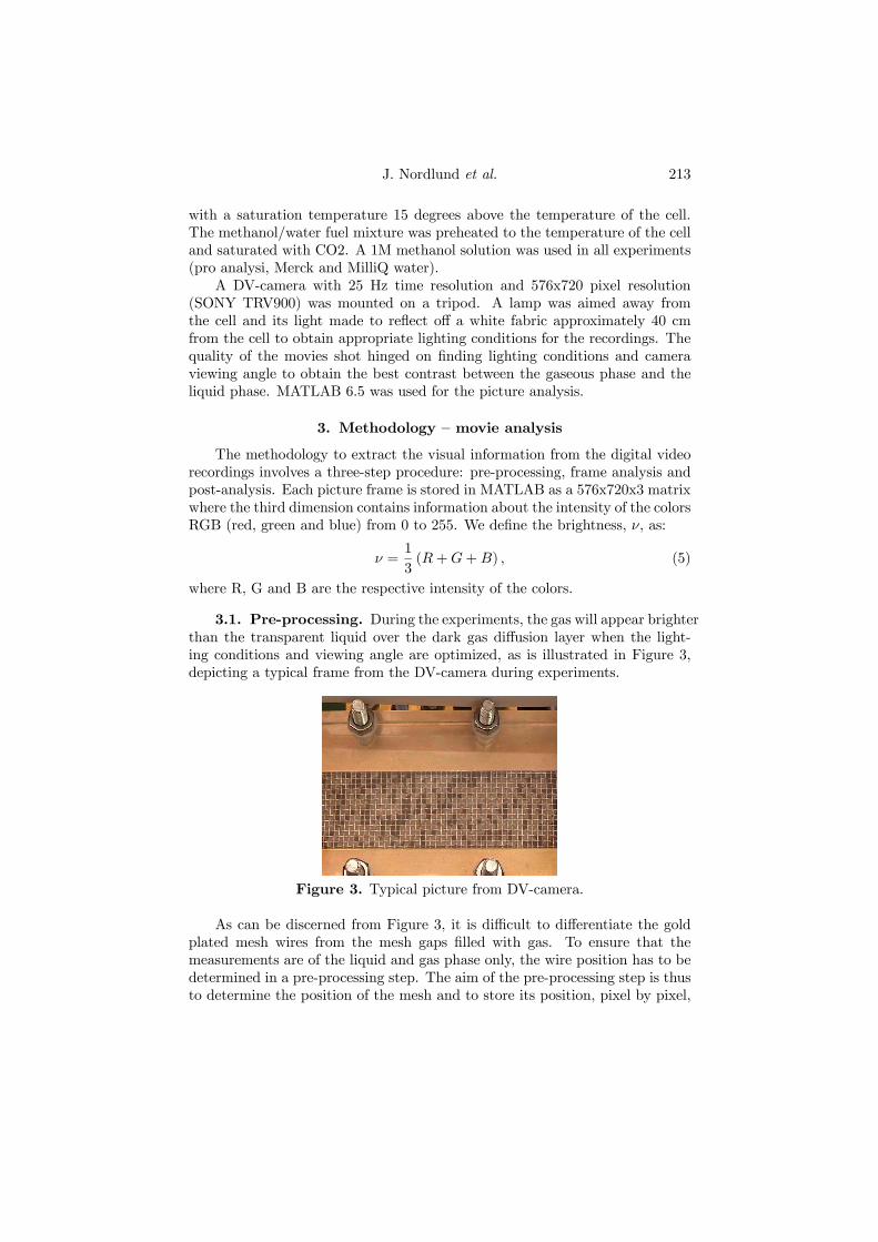
J. Nordlund et al. 213
with a saturation temperature 15 degrees above the temperature of the cell.The methanol/water fuel mixture was preheated to the temperature of the celland saturated with CO2. A 1M methanol solution was used in all experiments(pro analysi, Merck and MilliQ water).
A DV-camera with 25 Hz time resolution and 576x720 pixel resolution(SONY TRV900) was mounted on a tripod. A lamp was aimed away fromthe cell and its light made to reflect off a white fabric approximately 40 cmfrom the cell to obtain appropriate lighting conditions for the recordings. Thequality of the movies shot hinged on finding lighting conditions and cameraviewing angle to obtain the best contrast between the gaseous phase and theliquid phase. MATLAB 6.5 was used for the picture analysis.
3. Methodology — movie analysis
The methodology to extract the visual information from the digital videorecordings involves a three-step procedure: pre-processing, frame analysis andpost-analysis. Each picture frame is stored in MATLAB as a 576x720x3 matrixwhere the third dimension contains information about the intensity of the colorsRGB (red, green and blue) from 0 to 255. We define the brightness, ν, as:
ν =1
3(R+G+B) , (5)
where R, G and B are the respective intensity of the colors.
3.1. Pre-processing. During the experiments, the gas will appear brighterthan the transparent liquid over the dark gas diffusion layer when the light-ing conditions and viewing angle are optimized, as is illustrated in Figure 3,depicting a typical frame from the DV-camera during experiments.
Figure 3. Typical picture from DV-camera.
As can be discerned from Figure 3, it is difficult to differentiate the goldplated mesh wires from the mesh gaps filled with gas. To ensure that themeasurements are of the liquid and gas phase only, the wire position has to bedetermined in a pre-processing step. The aim of the pre-processing step is thusto determine the position of the mesh and to store its position, pixel by pixel,
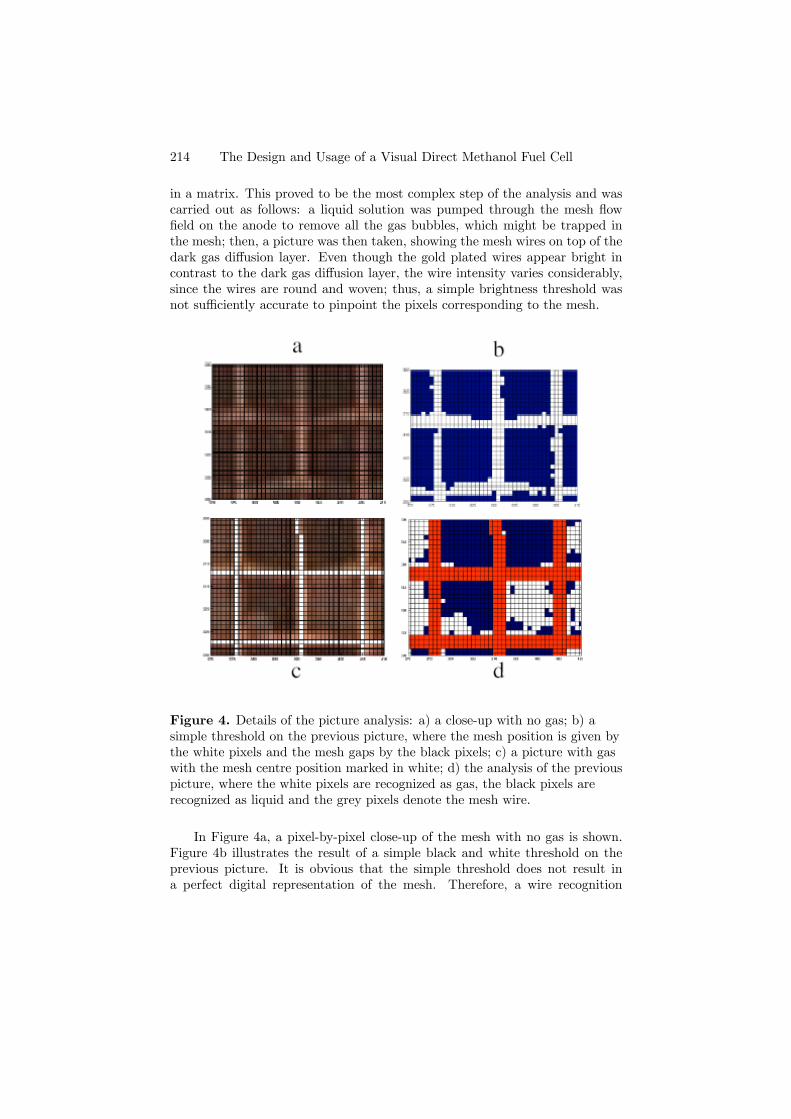
214 The Design and Usage of a Visual Direct Methanol Fuel Cell
in a matrix. This proved to be the most complex step of the analysis and wascarried out as follows: a liquid solution was pumped through the mesh flowfield on the anode to remove all the gas bubbles, which might be trapped inthe mesh; then, a picture was then taken, showing the mesh wires on top of thedark gas diffusion layer. Even though the gold plated wires appear bright incontrast to the dark gas diffusion layer, the wire intensity varies considerably,since the wires are round and woven; thus, a simple brightness threshold wasnot sufficiently accurate to pinpoint the pixels corresponding to the mesh.
Figure 4. Details of the picture analysis: a) a close-up with no gas; b) asimple threshold on the previous picture, where the mesh position is given bythe white pixels and the mesh gaps by the black pixels; c) a picture with gaswith the mesh centre position marked in white; d) the analysis of the previouspicture, where the white pixels are recognized as gas, the black pixels arerecognized as liquid and the grey pixels denote the mesh wire.
In Figure 4a, a pixel-by-pixel close-up of the mesh with no gas is shown.Figure 4b illustrates the result of a simple black and white threshold on theprevious picture. It is obvious that the simple threshold does not result ina perfect digital representation of the mesh. Therefore, a wire recognition

J. Nordlund et al. 215
program was implemented in MATLAB 6.5 to identify the centres of the meshwires. The identified grid centre is shown in Figure 4c. In this camera position,the grid is approximately three pixels wide; therefore, the grid removed fromthe processed pictures is three pixels wide with the centre taken as the centreposition of the mesh, as identified by the MATLAB program, see Figure 4d.
3.2. Frame analysis. It becomes obvious from the experiments that thegaps in the mesh normally either contain gas or liquid; a partially gas-filledmesh gap only occurs when a bubble is about to fill or leave a mesh gap. Whenstudying a snapshot of the movie, as in Figure 3, it is obvious that partially-filled mesh gaps occur significantly less frequently than mesh gaps that areeither completely filled with only gas or liquid. This observation allows asimplification of the frame analysis, since each gap thus can be considered tobe filled with either gas or liquid. We define a reduced binary M x N matrix,where M and N are the number of mesh gaps in the picture in the streamwiseand spanwise directions, respectively. As shown in Figure 4d, the mesh positionis known, and is removed from the full data matrix before the analysis. Thebrightness of every pixel in the mesh gap, see Figure 4c, is compared to athreshold value above and below which the pixel is considered white and below,respectively; the resulting matrix is shown in Figure 4d. A simple majority ofeither white or black pixels in a mesh gap could determine whether or not themesh gap should be considered as containing gas or liquid, although it wasfound that a higher precision was achieved, if the simple majority criterion wasabandoned. Instead, a 60% criterion was applied, where the mesh gap wasconsidered to “change” color only when more than 60% of the pixels in the gaphad done so.
4. Post-analysis
To ensure that the software captures and differentiates the liquid- fromthe gas-filled gaps, a verification image, produced by the software for everytenth frame, was visually examined. Figure 5 depicts such a verification image,where the recognition results are given as white (gas) or black (liquid) dots inthe actual picture.
Figure 5. The verification image for the automated gas recognition.
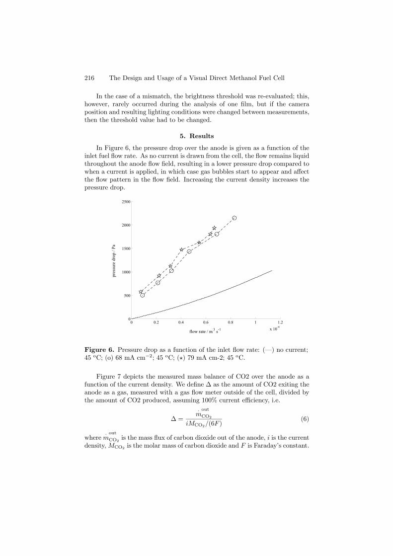
216 The Design and Usage of a Visual Direct Methanol Fuel Cell
In the case of a mismatch, the brightness threshold was re-evaluated; this,however, rarely occurred during the analysis of one film, but if the cameraposition and resulting lighting conditions were changed between measurements,then the threshold value had to be changed.
5. Results
In Figure 6, the pressure drop over the anode is given as a function of theinlet fuel flow rate. As no current is drawn from the cell, the flow remains liquidthroughout the anode flow field, resulting in a lower pressure drop compared towhen a current is applied, in which case gas bubbles start to appear and affectthe flow pattern in the flow field. Increasing the current density increases thepressure drop.
0 0.2 0.4 0.6 0.8 1 1.2x 10⁻⁶
0
500
1000
1500
2000
2500
flow rate / m 3 s-1
pres
sure
dro
p / P
a
Figure 6. Pressure drop as a function of the inlet flow rate: (–) no current;45 oC; (o) 68 mA cm−2; 45 oC; ( ) 79 mA cm-2; 45 oC.
Figure 7 depicts the measured mass balance of CO2 over the anode as afunction of the current density. We define ∆ as the amount of CO2 exiting theanode as a gas, measured with a gas flow meter outside of the cell, divided bythe amount of CO2 produced, assuming 100% current efficiency, i.e.
∆ =
·mout
CO2
iMCO2/(6F )(6)
where·mout
CO2is the mass flux of carbon dioxide out of the anode, i is the current
density,MCO2 is the molar mass of carbon dioxide and F is Faraday’s constant.

J. Nordlund et al. 217
20 30 40 50 60 70 800.45
0.5
0.55
0.6
0.65
0.7
0.75
0.8
0.85
0.9
0.95
∆
current density / mA cm - 2
Figure 7. Value of ∆ as a function of current density. Temperature is 45 oCand flow rates are (o) 1.3e 7 m3s-1 and (¤) 4.5e-7m3s-1.
0 20 40 60 80 100 120 140 1600.25
0.3
0.35
0.4
0.45
0.5
0.55
0.6
0.65
0.7
0.75
current density / mA cm -2
pot
entia
l / V
Temperature increasing
30 deg C
40 deg C
50 deg C
Figure 8. Polarization curve for T= 30, 40 and 50 oC at a fuel flow rate of4.4e-7 m3s−1 (—o—). The solid lines (–) denote experimental data from a 1cm2 DMFC with a MEA of identical composition at high stoichiometric flowat 30 and 50 oC [10].
For current densities lower than 25 mA cm−2, ∆ is less than 0.5, indicatingthat less than 50% of the CO2 produced exits the anode as a gas, even though
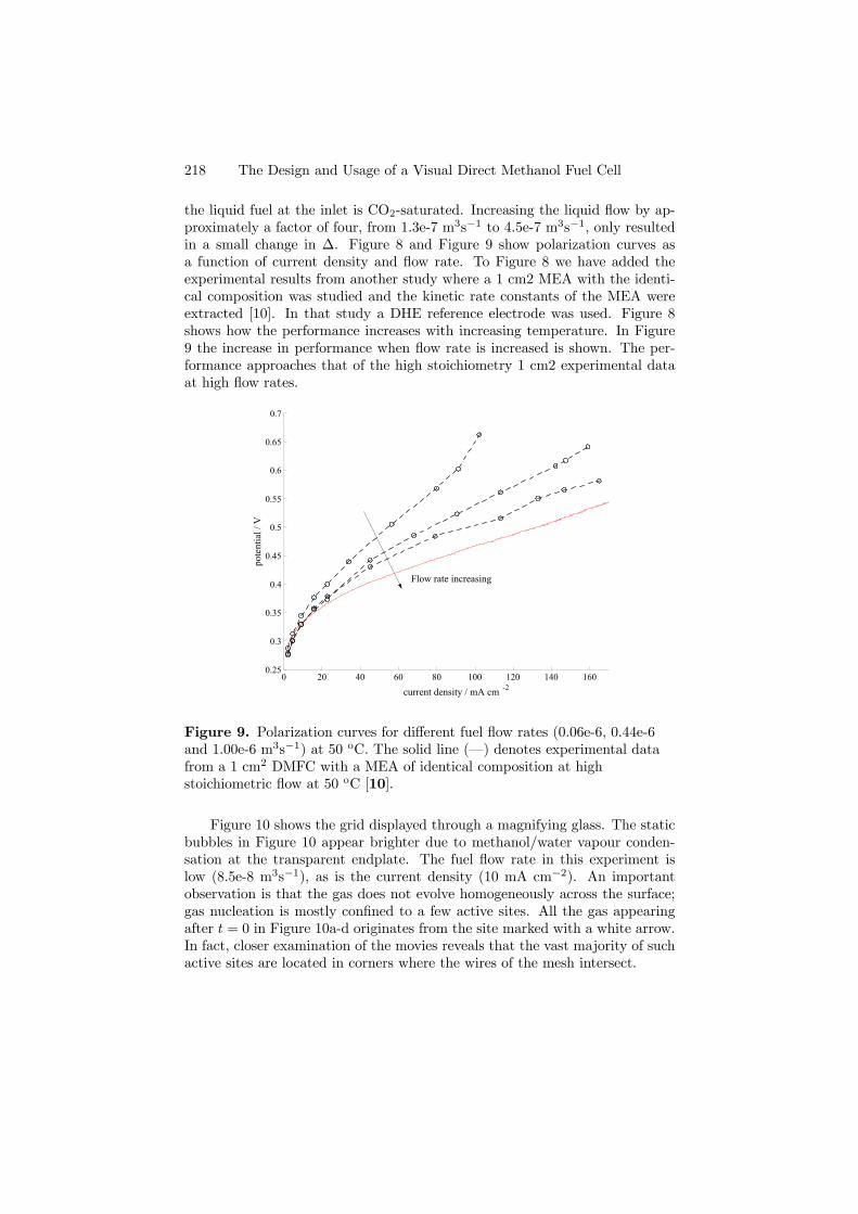
218 The Design and Usage of a Visual Direct Methanol Fuel Cell
the liquid fuel at the inlet is CO2-saturated. Increasing the liquid flow by ap-proximately a factor of four, from 1.3e-7 m3s−1 to 4.5e-7 m3s−1, only resultedin a small change in ∆. Figure 8 and Figure 9 show polarization curves asa function of current density and flow rate. To Figure 8 we have added theexperimental results from another study where a 1 cm2 MEA with the identi-cal composition was studied and the kinetic rate constants of the MEA wereextracted [10]. In that study a DHE reference electrode was used. Figure 8shows how the performance increases with increasing temperature. In Figure9 the increase in performance when flow rate is increased is shown. The per-formance approaches that of the high stoichiometry 1 cm2 experimental dataat high flow rates.
0 20 40 60 80 100 120 140 1600.25
0.3
0.35
0.4
0.45
0.5
0.55
0.6
0.65
0.7
current density / mA cm -2
pot
entia
l / V
Flow rate increasing
Figure 9. Polarization curves for different fuel flow rates (0.06e-6, 0.44e-6and 1.00e-6 m3s−1) at 50 oC. The solid line (–) denotes experimental datafrom a 1 cm2 DMFC with a MEA of identical composition at highstoichiometric flow at 50 oC [10].
Figure 10 shows the grid displayed through a magnifying glass. The staticbubbles in Figure 10 appear brighter due to methanol/water vapour conden-sation at the transparent endplate. The fuel flow rate in this experiment islow (8.5e-8 m3s−1), as is the current density (10 mA cm−2). An importantobservation is that the gas does not evolve homogeneously across the surface;gas nucleation is mostly confined to a few active sites. All the gas appearingafter t = 0 in Figure 10a-d originates from the site marked with a white arrow.In fact, closer examination of the movies reveals that the vast majority of suchactive sites are located in corners where the wires of the mesh intersect.
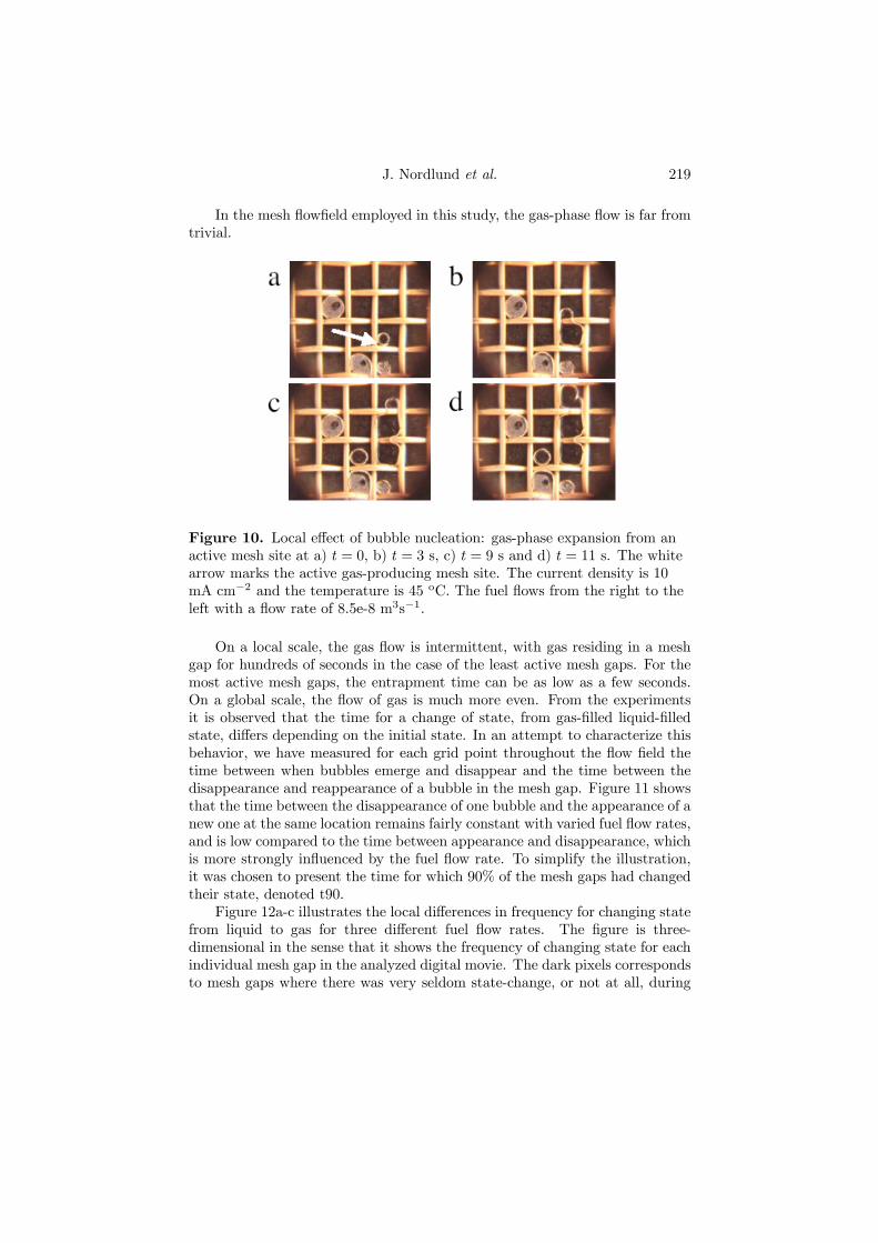
J. Nordlund et al. 219
In the mesh flowfield employed in this study, the gas-phase flow is far fromtrivial.
Figure 10. Local effect of bubble nucleation: gas-phase expansion from anactive mesh site at a) t = 0, b) t = 3 s, c) t = 9 s and d) t = 11 s. The whitearrow marks the active gas-producing mesh site. The current density is 10mA cm−2 and the temperature is 45 oC. The fuel flows from the right to theleft with a flow rate of 8.5e-8 m3s−1.
On a local scale, the gas flow is intermittent, with gas residing in a meshgap for hundreds of seconds in the case of the least active mesh gaps. For themost active mesh gaps, the entrapment time can be as low as a few seconds.On a global scale, the flow of gas is much more even. From the experimentsit is observed that the time for a change of state, from gas-filled liquid-filledstate, differs depending on the initial state. In an attempt to characterize thisbehavior, we have measured for each grid point throughout the flow field thetime between when bubbles emerge and disappear and the time between thedisappearance and reappearance of a bubble in the mesh gap. Figure 11 showsthat the time between the disappearance of one bubble and the appearance of anew one at the same location remains fairly constant with varied fuel flow rates,and is low compared to the time between appearance and disappearance, whichis more strongly influenced by the fuel flow rate. To simplify the illustration,it was chosen to present the time for which 90% of the mesh gaps had changedtheir state, denoted t90.
Figure 12a-c illustrates the local differences in frequency for changing statefrom liquid to gas for three different fuel flow rates. The figure is three-dimensional in the sense that it shows the frequency of changing state for eachindividual mesh gap in the analyzed digital movie. The dark pixels correspondsto mesh gaps where there was very seldom state-change, or not at all, during

220 The Design and Usage of a Visual Direct Methanol Fuel Cell
the measurement, whereas the brighter pixels corresponds to mesh gaps thatchange state between liquid and gas much more frequently.
0 1 2 3 4 5 6 7 8 9x 10⁻⁷
0
10
20
30
40
50
60
70
80
90
flow rate / m 3 s-1
time
t 90 /
s
Figure 11. Illustration for the change of state at 45 oC and 68 mA cm−2 asa function of fuel flow rate: (o) necessary time to observe disappearance andreappearance of a bubble in 90% of the mesh gaps, (¤) necessary time toobserve appearance and disappearance of a bubble in 90% of the mesh gaps.
Figure 12. Frequency for changing state from liquid to gas for recorded meshgaps. Each pixel corresponds to a physical gap in the mesh. The temperatureis 45 oC and the current density is 68 mAcm−2. The fuel flows from left toright and the rate is: a) 8.5e-8 m3s−1, b) 3.2e-7 m3s−1 and c) 8.0e-7 m3s−1.
Figure 13 show the spanwise average of the time-averaged gas saturationfor each individual mesh gap as a function of the streamwise position; the timeinterval used for averaging was approximately 240 — 300 s. Even though the

J. Nordlund et al. 221
data appears to be somewhat dispersed, the trend that the time averaged gassaturation increases along the streamwise axis of the fuel cell is clear. Figure13 also shows that a higher fuel flow rate reduces the gas saturation.
0 5 10 15 20 25 30 35 40 45 500.3
0.4
0.5
0.6
0.7
0.8
0.9
1
streamwise position
span
wis
e av
erag
ed g
as sa
tura
tion
Figure 13. Streamwise gas saturation at 45 oC and 68 mA cm−2. Fuel flowrates are (¤) 8.5e-8 m3s−1 and (o) 8.0 e-7 m3s−1. The dotted trend linecorresponds to the lower fuel flow rate. Trend lines were fitted withMATLAB.
6. Discussion
Figure 6 shows a considerable increase in pressure drop when a current isdrawn. This increase can be attributed to the carbon dioxide gas production,which takes place as a current is passed through the cell. The employed meshflow field traps the bubbles in the mesh gaps, as seen in Figure 12, resulting ina reduced cross section for liquid-phase flow. Taking an average gas saturationof about 0.7-0.8 from Figure 13 and assuming that the gas blocks the way forthe liquid, then the local liquid flow rate in the free passage in the mesh wouldincrease considerably, due to lessened free passage and increased tortuosity. Itis reasonable that this increase in local liquid flow rate leads to a substantialincrease in pressure drop.
At low current densities, less than 50% of the produced carbon dioxideis accounted for in the anode exhaust according to Figure 7. Since the fuelis saturated with CO2 before entering the cell, there are two possible reasonsfor this observation: mass transport through the membrane to the cathodeside or a low current efficiency for carbon dioxide production. The latter is
222 The Design and Usage of a Visual Direct Methanol Fuel Cell
less likely since the fraction accounted for in the exhaust approaches 100% athigher current densities. It has been show earlier that the concentration ofCO2 in the anode active layer may be well over the solubility limit, as thepores are too small to allow CO2 gas nucleation [6, 11]. This supersaturatedcarbon dioxide can travel one of two ways: through the membrane over to thecathode side, where the partial pressure of carbon dioxide is virtually zero,or through the gas diffusion layer, along the streamwise direction of the meshand through the anode outlet. The major contributions to the mass transferresistance on the anode side are due to: diffusion through the gas diffusionlayer to the mesh where CO2-saturated fuel flows and transport through themesh to the outlet. The latter should not be underestimated, as the fuel issaturated and the velocity of the gas, hindered by the mesh, is very low.
Qualitatively, the results shown in Figure 8 agree well with those in a sep-arate work, where the kinetics of the electrode were deduced in a 1 cm2 DMFC[10]. The agreement is best at low current densities (less than 20 mA cm−2),where depletion of methanol along the streamwise position is negligible be-cause of high stoichiometry. The observation in Figure 9 that the performanceat higher flow rates approaches the 1 cm2 cell data supports that conclusion.
None of the results displayed in Figure 6 to Figure 9 are unique for exper-iments with a visual cell. Nevertheless, by using a visual DMFC, the resultsmay be interpreted in the light of the specific knowledge obtained, thanks tothe data from the visual investigation. For instance, the increase in pressuredrop seen in Figure 6 can be directly linked to the observed stationary gasbubbles reducing the free passage for the flow of liquid fuel.
One of the most interesting observations in this work is that the gas (pro-duced in the active layer and transported through the gas diffusion layer) inthe flow field distributor is far from homogeneous. Figure 10 shows an activemesh cell and the surrounding passive cells. The movement of the gas from onemesh cell to the downstream adjacent cell is also shown. The fact that the vastmajority of such active sites are located in mesh corners, where wires intersect,is not very surprising, considering that the gas diffusion layer at those pointsis more compressed. This compression will result in reduced contact resistancebetween the mesh and the gas diffusion layer; in addition the mass transfer ofmethanol and carbon dioxide is enhanced.
As expected, there are fewer inactive mesh gaps and generally higher fre-quencies for state change from liquid to gas when the fuel flow rate is higher, asseen in Figure 12. Keeping the local differences shown in Figure 12 in mind, itis easier to understand the apparent randomness in Figure 13. Figure 13 showsthat the gas saturation increases in the streamwise direction of the fuel cell andthat the gas saturation decreases for higher fuel flow rates. These results ap-pear to make sense: the gas saturation should be higher along the streamwisedirection since gas is produced along the axis. In addition, the gas saturationshould be lower when liquid flow rate is higher, since the liquid is then moreeasily able to push the gas forward, and thereby preventing entrapment in themesh.

J. Nordlund et al. 223
To improve the performance of the DMFC, knowledge of the nature of thelimiting factors within the DMFC anode is important. Here modeling of theanode will play an important part. The methodology presented can play a vitalrole in the acquisition of the visual data needed to verify the two-phase flowmodels. A good model should not only be able predict polarization curves well;its two-phase predictions should also match experimental reality.
Some parameters that it will be of interest to vary in future experimentsand models are the flow matrix, surface tension and the gas-backing material.In addition, the influence of oscillating fuel pressure with different frequenciesand amplitudes, as well as operation in vertical mode, should be investigated.The methodology can also be used to provide knowledge about the CO2 concen-tration gradients in the system. For instance, by using a high speed DV-cameramore rapid phenomena, such as the implosion of bubbles that is observed whenthe current is interrupted, can be studied in more detail to give valuable insightinto the actual CO2 concentration gradients.
7. Conclusions
A visual DMFC system and a methodology to extract useful data fromDV-camera recordings were developed. From the experiments and analysis ofthe employed method the following can be concluded:
At low current densities, a large fraction of the carbon dioxide produced isnot transported out with the liquid flow, but rather transported through themembrane to the cathode side. The gas bubbles that form in the flow fieldtends not to move continuously: they nucleate, grow to the neighboring sitesand are finally swept away with the liquid flow. The fact that the bubbles are,in a sense, trapped in the mesh gaps leads to a sharp increase in pressure dropwhen a current is drawn, as compared to an all-liquid system.
Another important observation was that the formation of gas bubbles wasnot uniform: gas bubbles tend to form at several active mesh gaps, which aremore or less randomly located in the mesh. These active mesh gaps have a largeinfluence on the result when studying gas saturation or frequency of changingstate between liquid and gas; moreover, the results appear to be random. Aconsequence is that a visual cell with a mesh flow field should have more meshgaps in either the spanwise nor the streamwise direction than cell used in thiswork to decrease the uncertainty in the data from the random positions of themore active mesh gaps.
Despite the randomness of the local data, a clear trend can be seen: thegas saturation increases along the streamwise direction in the fuel cell. The gassaturation and how it changes along this axis is an important example of datathat can be used to verify two-phase flow models of the anode.
The final conclusion is that the combination of a visual DMFC and a DV-camera is a very simple, affordable, yet powerful, tool and methodology tostudy and improve the direct methanol fuel cell.

224 The Design and Usage of a Visual Direct Methanol Fuel Cell
Acknowledgements
The financial support from the Swedish Foundation for Strategic Environ-mental Research, MISTRA, and from the Swedish National Energy Adminis-tration is gratefully acknowledged. The work was done within the frameworkof the Jungner Center. J. Nordlund gratefully acknowledges the scholarshipfrom the Ernst Johnson foundation.

Bibliography
[1] E. Birgersson, J. Nordlund, H. Ekström, M. Vynnycky, G. Lindbergh, J. Elec-trochem. Soc., 150, (2003) A1368
[2] P. Argyropoulos, K. Scott, W.M. Taama, J. Appl. Electrochem., 29, (1999) 661[3] K. Sundmacher, K. Scott, Chem. Eng. Sci., 54, (1999) 2927[4] P. Argyropoulos, K. Scott, W.M. Taama, Electrochimica Acta, 44, (1999) 3575[5] K. Scott, P. Argyropoulos, P. Yiannopoulos, W.M. Taama, J. Appl. Electrochem.,
31, (2001) 823[6] J. Nordlund, G. Lindbergh, J. Electrochem. Soc., 149, (2002) A1107[7] C. Crow, M. Sommerfeld, Y. Tsuji, Multiphase Flow with Droplets and Particles,
Boca Raton, CRC Press, 1998[8] Flow Visualization and Image Analysis, F.T.M. Nieuwstadt ed., Delft, The Netherlands,
1993[9] P. Boissonneau, P. Byrne, J. Appl. Electrochem., 30, (2000) 767[10] J. Nordlund, G. Lindbergh, submitted to J. Electrochem. Soc.[11] J. Nordlund, A. Roessler, G. Lindbergh, J. Appl. Electrochem., 32, (2002) 259
225


Paper 7


Reduced Two-Phase Model for Analysis of theAnode of a DMFC
E. Birgerssona, J. Nordlundb, M. Vynnyckya, C. Picardc and G.Lindberghb
aDepartment of Mechanics, FaxénLaboratoriet, The Royal Institute of Technology,SE-100 44, Stockholm, SwedenbDepartment of Chemical Engineering and Technology, Applied Electrochemistry,The Royal Institute of Technology, SE-100 44 Stockholm, SwedencPresent address: LEGI, Ecole Nationale Supérieure d’Hydraulique et de Mécaniquede Grenoble, Saint Martin d’Hères, France
Abstract. An isothermal two-phase ternary mixture model that takes into ac-count conservation of momentum, mass and species in the anode of a direct methanolfuel cell (DMFC) is presented and analysed. The slenderness of the anode allows aconsiderable reduction of the mathematical formulation, without sacrificing the essen-tial physics. The reduced model is then verified and validated against data obtainedfrom an experimental DMFC outfitted with a transparent end plate. Good agreementis achieved. The effect of mass transfer resistances in the flow field and porous back-ing are highlighted. It is found that at a temperature of around 30oC, a one-phasemodel predicts the same current density distribution as a more sophisticated two-phase model. Analysis of the results from the two-phase model, in combination withthe experiments, results in a suggestion for an optimal flow field for the liquid-fedDMFC.
Key words. DMFC; two-phase; multiphase mixture, validation.
1. Introduction
The direct methanol fuel cell (DMFC) constitutes an attractive alternativeto classical power sources for many low power applications, such as mobilephones and laptops. Some of the promising features include high power andenergy densities, low emissions, operation at or near ambient conditions, fastand convenient refuelling and a potentially renewable fuel. Compared to themore traditional hydrogen-fed polymer electrolyte fuel cell, the DMFC has theadvantage of a direct liquid fuel feed: a liquid fuel has a higher energy densitythan a gaseous fuel and the excess fuel is more easily recycled within the system.The fuel, methanol, enters the flow field, see Figure 1, on the left and is oxidizedin several steps at the anode active layer, with the overall reaction being
CH3OH +H2O→ CO2 + 6H+ + 6e−. (1)
The DMFC can be operated with vaporized fuel, but it is the simpler liquid fu-elled mode of operation that attracts most attention today. Liquid fed DMFCsare operated at relatively low temperatures (< 100oC), where the producedcarbon dioxide at the anode forms a gas when the local concentration exceeds

230 A Reduced Model for Analysis of the Anode of a DMFC
the solubility limit and conditions required for nucleation are fulfilled. Due tothe low solubility, this can occur even at low current densities [1], whence thefuel flow will be two-phase in the anode flow matrix.
L
y
x
hf
hp
UinNet-type flow field
Porous backing
Active layerFigure 1. A schematic of the anode side of a DMFC.
As it is not feasible to quantify the physical processes that occur in theDMFC anode directly, because of the small scales involved, theoretical mod-elling provides an important tool for elucidating the main transport mechanismsand limitations in the anode. Several mathematical models have been devel-oped in an effort to capture and describe the physical processes in the anode,including the electrochemistry [1-19]. Most of these consider mass transfer inboth the gas-backing layer and the active layer [1,5-9,12,13,14-17,19], whereascomparatively few consider streamwise effects [1,5,8,18].
The carbon dioxide gas is usually neglected in DMFC modelling literature,even though the evolution of gas at the anode can be observed in most practicalDMFC applications. Most recently, however, two models that consider coex-isting gas and liquid phases have been published [18,19]. Wang and Wang [18]apply a multiphase mixture theory for porous media [20] to the porous back-ings, active layers of both the anode and cathode as well as the membrane ofa two-dimensional DMFC, and treat the flow channels on the anode side witha drift flux model to account for the gas slug flow. They use a simplified ex-pression for the anode kinetics: a Tafel slope with a reaction order that is zeroor one, depending on whether the methanol concentration exceeds a prescribedthreshold value. The model by Divisek et al. [19] is also two-dimensional, butfor a cross-section at a given streamwise position, and is limited to the porousbackings, active layers and membrane of the cell. Common to both of these two-phase models is that they are only validated against global polarization curves;thus, there are no local experimental details about the two-phase flow, suchas, e.g., the amount of gas in the flow channels. Such polarization curves areill-suited for validating the increasing number of constitutive relations that arenecessary to close the governing equations when proceeding from a one-phasetreatment to a model that handles two-phase flow.

E. Birgersson et al. 231
In this work we focus on the anode side of the DMFC and adopt the sameanalytic approach using scaling arguments and elementary asymptotic tech-niques as in our previous work [1], where a liquid-phase model was analyzed.Similar to the one-phase model, we will show that the complexity of the gov-erning equations can be reduced, without sacrificing any essential physics. Inaddition to reducing the computational cost, the analysis provides an insightinto the dominating transport mechanisms a priori to any computations, aswell as allowing a reduction of the considerable number of dimensional pa-rameters to a few dimensionless numbers. Experiments with a visual DMFCprovide local information about the amount of gas in the flow field at the anode,pressure drops and anode polarization curves.
The mathematical model is similar to that of Wang and Wang [18], andis based on the multiphase mixture theory derived by [20] for both the porousbacking and the flow field, in our case a net. We consider laminar two-phase flowin the anode in the streamwise and normal directions, see Figure 1, governed bythe generalized Darcy law in both the net and the porous backing, coupled withmulticomponent mass transfer in the liquid and gas phase for carbon dioxide,water and methanol, assuming equilibrium conditions throughout. The liquidflow can be treated as a dilute mixture. For the active layer, a model developedby Nordlund et al. [21] accounting for ionic conductivity, pore diffusion, and thecomplex methanol oxidation kinetics, is applied as a boundary condition. In itssimplified form, the model, which includes all porous effects in the active layer,is reduced to a simple kinetic expression that is valid in the temperature range303-343 K, the potential range 0.25-0.7 V vs DHE and 0.1-4 M methanol con-centration. Isothermal conditions are assumed, which is reasonable consideringthe low current densities. Non-dimensionalisation, followed by a scale analysis,allows for considerable reduction of the mathematical formulation: the veloc-ity field in the net decouples from the rest of the flow and can be solved for apriori to any computations; the flow in the porous backing is at leading orderin the normal direction only. The reduced model is then solved numericallywith a Keller Box scheme and verified against a commercial code that solvesfor the full set of governing equations, boundary conditions and constitutiverelations. Experiments performed with a DMFC equipped with a transparentend plate on the anode are outlined and the reduced model is validated againstexperimentally measured pressure drop, gas saturation and anode polarizationcurves. Good agreement between experimental data and the model are shown.Results from a parameter study are discussed and conclusions are drawn.
2. Mathematical formulation
We consider a slender 3D geometry consisting of a net-type flow field ad-jacent to the porous backing in the anode. The porous nature of the flow fieldand porous backing allows a reduction in dimensionality, since the changes independent variables in the spanwise direction are negligible due to slip condi-tions and no flux that can be invoked at the left and right walls of the anode.

232 A Reduced Model for Analysis of the Anode of a DMFC
The geometry that we need to resolve can thus be reduced to the streamwise(ex) and normal direction (ey), as shown in Figure 1.
For a liquid-fed anode, the flow through the anode will remain liquid aslong as no current is drawn from the cell. As soon as a current is drawn,carbon dioxide is produced from the oxidation reaction at the active layer ofthe anode. Provided that the carbon dioxide partial pressure is sufficiently highand nucleation can occur, gas will evolve. The liquid fuel, comprising dilutemethanol in water, is usually recirculated, whence it is normally saturated withcarbon dioxide. Incorporating these effects calls for a two-phase model, whereconservation of mass, momentum and species are treated. For this purpose,we apply a mixture formulation, derived by [20]. The ternary gas and liquidphases, comprising carbon dioxide, methanol and water, are assumed to be inequilibrium. The porous effects and the inherent electrochemistry in the activelayer is, as in [1], treated as a boundary condition, yet changes in potential andconcentrations inside the active layer are still captured, and can, if so desired,be computed a posteriori. This was accomplished by parameter adaption toa more detailed active layer model in [21]. In addition, we treat the anode asisothermal.
2.1. Basics of two-phase flow in porous media. Some basic conceptsare essential for two-phase modeling, the most important of which are summa-rized here, see e.g., [22] and [23] for further details.
The amount of gas and liquid in a representative elementary volume isgiven by the saturation
s(l) =V(l)
V(l) + V(g) , s(g) =
V(g)V(l) + V(g) , (2)
where s(k) and V(k) are the saturation and volume of phase k, respectively. Inaddition, s(l) + s(g) = 1. The intrinsic and superficial averages of a propertyφ(k) (scalar, vector, tensor) of the phase k are defined asD
φ(k)E(k)
=1
V(k)ZV(k)
φ(k)dV,Dφ(k)
E=1
V
ZVφ(k)dV. (3)
We will save on notation in the forthcoming analysis, by omitting h.i and re-ferring to the liquid saturation as s.
2.2. Governing equations. We solve for the continuity of mass and mo-mentum of the liquid and gas phase, given by
∇ · (ρv) = 0, (4)
∇p = −µκv+ ρkg, (5)
where ρ,v = (u, v), p, µ and ρk are the mixture density, the mixture veloc-ity, the mixture pressure, dynamic mixture viscosity and kinematic mixturedensity, respectively, κ is the absolute permeability and g is the gravitationalacceleration. When referring to the properties of the individual liquid and gas
E. Birgersson et al. 233
phases, we will use the superscripts (l) and (g), respectively. The mixture vari-ables are summarized in Appendix A. For later use, we note that the mixtureformulation for the momentum equation, Eq. 5, contains the liquid pressure,p(l), given by
∇p(l) = − µ(l)
κκ(l)rel
v(l) + ρ(l)g, (6)
Species transfer is accounted for by
∇ ··NMeOH
NCO2
¸= 0, (7)
with·NMeOH
NCO2
¸= ρv
Ãλ(l)
M (l)
"x(l)MeOH
x(l)CO2
#+
λ(g)
M (g)
"x(g)MeOH
x(g)CO2
#!−Ã
sρ(l)γ hMi(l)¡M (l)
¢2"∇x(l)MeOH∇x(l)CO2
#+(1− s)ρ(g)γ hMi(g)¡
M (g)¢2
"∇x(g)MeOH∇x(g)CO2
#!+Ã
1
M (l)
"x(l)MeOH
x(l)CO2
#− 1
M (g)
"x(g)MeOH
x(g)CO2
#!λ(l)λ(g)κρ
µ
³∇p(c) +
³ρ(l) − ρ(g)
´g´;
(8)
here, NMeOH and NCO2 are the total molar fluxes of methanol and carbondioxide, hMi(l,g) , λ(l) and λ(g) are the diffusion tensors and mobilities of theliquid and gaseous phase, p(c) is the capillary pressure, p(g) is the pressure inthe gas phase, ρ(k) and x
(k)i are the density and mole fractions of species i
in phase k, respectively. M (l,g) are the mean molecular masses and diffusiontensors for the liquid and gas phases, respectively. and are given by
M (l,g) = x(l,g)MeOHMMeOH + x
(l,g)CO2
MCO2 + x(l,g)H2O
MH2O. (9)
The total molar fluxes Ni are written in a compact form, to be read as twoequations, one for methanol and the other for carbon dioxide, which are coupledthrough the diffusion tensors hMi(l,g) .
The capillary pressure, p(c), is defined as
p(c) = p(g) − p(l), (10)
and the mixture pressure, p, as
∇p = ∇p(l) + λ(g)∇p(c). (11)
2.3. Boundary conditions. At the inlet (x = 0, 0 ≤ y ≤ hf ) we specifythe inlet velocity, liquid saturation and phase compositions:
u = U in, x(l)MeOH = x
(l),inMeOH, s = sin. (12)
At the upper net wall (0 ≤ x ≤ L, y = hf ), there is no normal flow and nocomponent flux:
v =NMeOH · ey =NCO2 · ey = 0. (13)
234 A Reduced Model for Analysis of the Anode of a DMFC
At the outlet (x = L, 0 ≤ y ≤ hf), we set no diffusive componental flux in thestreamwise direction and a reference pressure:
∂x(l)MeOH
∂x=
∂s
∂x= 0, p(l) = pref . (14)
At the vertical walls of the porous backing (x = 0, L, −hp ≤ y ≤ 0), we haveno normal flow and no mass flux:
u =∂x
(l)MeOH
∂x=
∂s
∂x= 0. (15)
At the interface between the porous backing and the net (0 ≤ x ≤ L, y = 0),we prescribe continuity of liquid saturation, the mole fraction of methanol, thenormal velocity and pressure as well as continuity of the carbon dioxide andmethanol fluxes:
s|y=0+ = s|y=0− , x(l)MeOH
¯y=0+
= x(l)MeOH
¯y=0−
, (16)
v|y=0+ = v|y=0− , p|y=0+ = p|y=0− , (17)
NMeOH|y=0+ ·ey = NMeOH|y=0− ·ey, NCO2|y=0+ ·ey = NCO2
|y=0− ·ey. (18)
At the active layer/porous backing interface (0 ≤ x ≤ L, y = −hp), the activelayer is reduced to a boundary condition, with the total mass flux ρv =
PNi·ey
and component fluxes given by
ρv = − i
6F((1 + 6αH2O)MH2O + (1 + 6αMeOH)MMeOH −MCO2)
− ρ(l)D(m)MeOHMMeOH
M (l)
³x(l)MeOH − x
(l),cathodeMeOH
´hm
, (19)
NMeOH · ey = −i
6F(1 + 6αMeOH)−
ρ(l)D(m)MeOH
M (l)
³x(l)MeOH − x
(l),cathodeMeOH
´hm
, (20)
NCO2 · ey =i
6F, (21)
where x(l),cathodeMeOH is the mole fraction of methanol in the liquid phase at theactive layer of the cathode. The first term on the RHS of Eq. 20 accounts forthe methanol consumed in the oxidation reaction, Eq. 1, and the methanoldepletion due to the electroosmotic drag through the membrane. Permeationof methanol through the membrane via diffusion is approximated by the secondterm on the RHS, where we have assumed a linear profile for methanol acrossthe membrane.
E. Birgersson et al. 235
2.4. Constitutive relations. The capillary pressure is approximated by
p(c) = p(b)J(s), (22)
where p(b) is the breakthrough pressure and J(s) = J(s)/J(s(b)) is a Leverettfunction, scaled with the corresponding Leverett function for the breakthroughliquid saturation, s(b), given by d2J/ds2 = 0 [24]. Since we do not have anyquantitative information regarding the capillary pressures of the net and porousbacking, we will assume the capillary pressure to be ∼ O(τ
pγ/κJ(s(b))), i.e.
103 Nm−2 in the net and 104 Nm−2 in the porous packing. Wang and Wang[18] and Scott et al. [7] apply a similar expression for the capillary pressure.Divisek et al. [19] derive another expression for the capillary pressure, wherep(c) ∼ O(10) Nm−2; clearly, there is a large discrepancy between the capillarypressures of different models. We will see later how such a low capillary pressureaffects the model we derive here.
The relative permeabilities are taken to be
κ(l)rel = κ
(l)rel(s), (23a)
κ(g)rel = κ
(g)rel (s). (23b)
Due to lack of experimental data at this stage the following empirical relation-ships will be used:
J(s) = 1.417(1− s)− 2.120(1− s)2 + 1.263(1− s)3, (24)
κ(l)rel(s) = sn, (25)
κ(g)rel (s) =
½ε1(1− s)(n+ε2), in the net(1− s)(n+ε2), in the porous backing
. (26)
We will later find n, ε1 and ε2 from parameter adaption to liquid saturationprofiles and pressure drops obtained with a visual cell [25]. The net-type flowfield, described in the section on the experimental setup, exhibited a high re-sistance towards the gas flow, more or less trapping the gas bubbles in eachmesh of the net, which we try to capture by introducing ε1 to the relativepermeability of the gas in the net.
Assuming equilibrium between the gas and liquid phase, we can write
x(g)MeOH = x
(g)MeOH
³p(g), T, x
(l)MeOH
´, (27)
x(g)CO2
= x(g)CO2
³p(g), T, x
(l)MeOH
´, (28)
x(l)CO2
= x(l)CO2
³p(g), T, x
(l)MeOH
´; (29)
these functions are derived in appendix B.The liquid dynamic viscosity is given by [26] as
µ(l) (T ) = 0.6612(T − 229)−1.562. (30)
236 A Reduced Model for Analysis of the Anode of a DMFC
The multicomponent diffusion tensors are as given by [27],
M(l,g) =MH2O
ÃD(l,g)MeOH,H2O
D(l,g)MeOH,H2O
D(l,g)CO2,H2O
D(l,g)CO2,H2O
!
−Ã
0 MCO2D(l,g)MeOH,CO2
MMeOHD(l,g)CO2,MeOH
0
!, (31)
with
D(l,g)ij = D(l,g)ij
1 + x(l,g)k
h(Mk/Mj)D(l,g)ik −D(l,g)ij
ix(l,g)i D(l,g)jk + x
(l,g)j D(l,g)ik + x
(l,g)k D(l,g)ij
, i, j, k = 1, 2, 3 (i 6= j).
(32)The temperature and gas pressure dependence of the binary diffusion coeffi-cients for the gas phase are [28]
D(g)ij (T, p(g)) =p(g)0
p(g)
µT
T0
¶ 32
D(g)ij (T0, p(g)0 ), (33)
assuming an ideal gas. For the liquid phase, we only need to consider [31]
D(l)MeOH,H2O
(T ) =Tµ(l)(343 K)343µ(l)
D(l)MeOH,H2O
(343 K), (34)
D(l,g)CO2,H2O
(T ) = 1.173× 10−16 × 2.260.5 × 180.5T
0.0340.6µ(l), (35)
since the liquid phase is dilute. In the membrane, Nafion 117, we use
D(m)MeOH(T ) = 4.9× 10−10 exp
·2436
µ1
333− 1
T
¶¸, (36)
for the methanol diffusion from the anode to the cathode side [29].The total superficial mass diffusivity tensor, accounting for both molecular
diffusion and dispersion, is approximated with a Bruggemann relationship,
γ hMi(l,g) = γ32M(l,g). (37)
We treat the liquid as incompressible, and furthermore take its density,ρ(l), to be that of pure water. For the density of the gas phase, we use theconstitutive relation for an ideal gas, i.e.
ρ(g)(T, p(g),M (g)) =p(g)M (g)
RT. (38)
The electroosmotic drag for methanol is assumed to be given by αMeOH =
x(l)MeOHαH2O [7].Henry’s constant HCO2 , which relates the amount of carbon dioxide in the
liquid and gas phase, is a function of temperature [30]
HCO2(T ) = exp(4.8 + 3934.3T−1 − 941290.2T−2)× 105, (39)
valid for 273-353 K and 1 atm.

E. Birgersson et al. 237
3. Electrokinetics and the active layer
The local current density at the active layer, i, is given by [21] as
i(x(l)MeOH, T,M
(l), EA) =exp
¡αAFRT (EA − EA)
¢1 +
exp³αAF
RT (EA−EA)´
ilim
, (40)
where
EA = c1 − c2T, (41)
ilim = tanh
x(l)MeOH
¯y=−hp
ρ(l)
M (l)¯y=−hp c3
µEAc4
¶ϑ ¡c5T
2 − c6T + c7¢, (42)
ϑ = c8 tanh
x(l)MeOH
¯y=−hp
ρ(l)
M (l)¯y=−hp c9
; (43)
in addition, EA is the anode potential measured at the active layer/membraneinterface versus a DHE reference electrode (EA = 0.2 − 0.7 V [21]), αA is ameasured Tafel slope , and ci are experimentally fitted parameters (see TableI).
The kinetic equation, Eq. 40, is taken from an earlier work [21] and includeslosses in the porous electrodes due to limited ionic conductivity and limitationsin mass transfer. The equation is valid in the range 303-343 K and 100-4000mol m−3 methanol concentration (mole fractions in the range 1.8e-3 to 7.4e-2),and is validated against experimental data for the whole range of validity. Theelectrode used in this work has identical composition to that used to derive thecurrent density expression, Eq. 40.
Table I. Data for electrokinetics.Constant Value UnitsαA 0.65 -c1, c2, c3 1.58, 0.0045, 2000 V, V K−1,m3mol−1
c4, c5, c6 0.7, 3.732, 2156.2 V, A m−2K−2,A m−2K−1
c7, c8, c9 313607, 1.5, 1000 A m−2,-, m3mol−1

238 A Reduced Model for Analysis of the Anode of a DMFC
4. Analysis
Non-dimensionalisation.- We introduce
ex =x
L, ey = y
L,DfME(g) = hMi(g)£
D(g)¤[M ]
,DfME(l) = hMi(l)£
D(l)¤[M ]
,
ev =v
U in, ev(l) = v(l)
U in, ev(g) = v(g)
U in, Mi =
Mi
[M ], M(l,g) =
M (l,g)
[M ],
ep(c) =p(c)
p(b)f
, ep = (p− pref)κf[µ]U inL
, ep(g) = p(g) − pref
∆p(g), ep(l) = p(l) − pref
∆p(l),
eρ(g) =ρ(g)£ρ(g)
¤ , eρ = ρ
[ρ], eρk = ρk
[ρ], µ =
µ
[µ], eNMeOH =
NMeOH[M ]
[ρ]U in,
eNCO2 =NCO2 [M ]
[ρ]U in, eD(l) =
D(l)
[D(l)], I = i
[i].
At this stage, [ρ] ,£ρ(g)
¤, [µ] , [M ], [i], ∆p(g), ∆p(l) remain unknown.
Recognizing that the liquid mixture is dilute, i.e. x(l)MeOH, x
(l)CO2
¿ x(l)H2O
,
we obtainM(l) = 1 by choosing [M ] = MH2O and the diffusion tensor for theliquid phase reduces to
eD(l) =
" eD(l)MeOH,H2O
0
0 eD(l)CO2,H2O
#.
Now, since the liquid saturation s ∼ 1 at the inlet, we chose to scale the mixtureproperties with the corresponding liquid scales, i.e.
[ρ] = ρ(l), [µ] = µ(l).
The scale for the liquid pressure drop can be inferred from Eq. 6 as ∆p(l) =µ(l)U inL/κ. The scale for the current density expression can be estimatedas [i] = i(x
(l),inMeOH), and gives the current density that we would obtain with
negligible mass transfer resistance in the net and porous backing, i.e. in an‘ideal’ anode.
In addition, the following dimensionless numbers are defined:
Re =ρ(l)U inL
µ(l), Sc(g) =
µ(g)£ρ(g)
¤ £D(g)
¤ µ(l)µ(g)
, Sc(l) =µ(l)
ρ(l)£D(l)
¤ ,Sc(c) =
¡µ(l)¢2
κfρ(l)p(b)f
, Λ1 =[i][M ]
ρ(l)U inF, Λ2 =
D(m)MeOHx
(l),inMeOH
U inhm,
Ca =µ(l)U inL
p(b)f κf
, Gl =ρ(l)gL
p(b)f
, Gr =µ(l)U in
ρ(l)gκf,
where Re, Sc(c,g,l), Λ, Ca, Gl and Gr are the Reynolds, Schmidt, Damköhler,capillary, gravillary and gravitary numbers, respectively. The capillary numberCa and the gravitary numberGr relate the viscous pressure drop to the capillary
E. Birgersson et al. 239
pressure and gravitational pressure, respectively, and the gravillary number Glgives the ratio of the gravitational pressure to the capillary pressure [24]. Toobtain a compact notation, we also introduce χp = χκ = 1 in the net and in
the porous backing χp = p(b)p /p
(b)f and χκ = κf/κp.
First, we observe from Eq. 97 that, since£ρ(g)
¤¿ ρ(l), we have ρ = s, as
given in Eq. (97). Then, dropping the tildes, we arrive at
∇ · (sv) = 0, (44)
∇p = −µχκv−Gr−1ρkey, (45)
∇ ·Ãsv
Ãλ(l)
"x(l)MeOH
x(l)CO2
#+
λ(g)
M(g)
"x(g)MeOH
x(g)CO2
#!!=
∇ ·(sγ
32D(l)
ReSc(l)
"∇x(l)MeOH∇x(l)CO2
#+(1− s)ρ(g)γ
32M(g)
ReSc(g)¡M(g)
¢2"∇x(g)MeOH∇x(g)CO2
#)
−∇·(
χpχ−1κ
ReSc(c)
Ã"x(l)MeOH
x(l)CO2
#− 1
M(g)
"x(g)MeOH
x(g)CO2
#!λ(l)λ(g)s
µ
³∇p(c) −Gley
´).
(46)
The capillary pressure is now
p(c) = J(s), (47)
and the definition of the capillary pressure, Eq. 10, yields
∆p(g)p(g) = p(b)f χpJ +∆p
(l)p(l), (48)
whence we are required to chose ∆p(g) = max(p(b)f χp,∆p
(l)). For the cases
considered here, p(b)f χp & ∆p(l), thus ∆p(g) = p(b)f χp. Now, choosing the gas
density scale as hρ(g)
i=[M ]pref
RT, (49)
gives
ρ(g) =
Ã1 +
Ãp(b)f χppref
J +∆p(l)
prefp(l)
!!M(g). (50)
The boundary conditions are now
u = 1, x(l)MeOH = x
(l),inMeOH, s = sin at x = 0, 0 ≤ y ≤ hf/L; (51)
v =∂x
(l)MeOH
∂y=
∂s
∂y= 0 at 0 ≤ x ≤ 1, y = hf/L; (52)
p(l) = 0,∂x
(l)MeOH
∂x=
∂s
∂x= 0 at x = 1, 0 ≤ y ≤ hf/L; (53)
u =∂x
(l)MeOH
∂x=
∂s
∂x= 0 at x = 0, 1, − hp/L ≤ y ≤ 0; (54)
240 A Reduced Model for Analysis of the Anode of a DMFC
At the interface between the porous backing and the net (0 ≤ x ≤ 1, y = 0),
s|y=0+ = s|y=0− , x(l)MeOH
¯y=0+
= x(l)MeOH
¯y=0−
, (55)
v|y=0+ = v|y=0− , p|y=0+ = p|y=0− , (56)
NMeOH|y=0+ ·ey = NMeOH|y=0− ·ey, NCO2 |y=0+ ·ey = NCO2 |y=0− ·ey. (57)The boundary conditions at the active region (0 ≤ x ≤ 1, y = −hp/L) are now
sv = −Λ1IΦ6− Λ2MMeOH
³x(l)MeOH − x
(l),cathodeMeOH
´x(l),inMeOH
, (58)
with Φ = ((1 + 6αH2O)MH2O + (1 + 6αMeOH)MMeOH −MCO2) , and
NMeOH · ey = −Λ1I6(1 + 6αMeOH)− Λ2
³x(l)MeOH − x
(l),cathodeMeOH
´x(l),inMeOH
, (59)
NCO2· ey =
Λ1I6
. (60)
4.1. Magnitude of dimensionless numbers. Typical scales are [i] ∼103 Am−2,
£D(g)
¤∼ 10−5 m2s−1,
£D(l)
¤∼ 10−9 m2s−1, ∆p(l) ∼ 300 Nm−2.
The remaining parameters are listed in Table II. The dimensionless numbersare Re ∼ 2 × 10³, Sc(g) ∼ 80, Sc(l) ∼ 100, Sc(c) ∼ 2 × 10⁻⁴,Λ1 ∼ 4 × 10⁻⁵,Λ2 ∼ 4 × 10⁻⁶, Ca ∼ 0.3, Gr ∼ 0.3, Gl ∼ 1, χp ∼ 10 (porous backing),χκ ∼ 2 × 10³ (porous backing). We have so far scaled with respect to thelength L of the anode and we see that: ReSc(g) À 1, ReSc(l) À 1, which meansthat convection dominates over diffusion for the species transfer; ReSc(c) ∼10−1, which implies that the capillary diffusion is somewhat stronger than theconvective transport, if λ(l,g) are not too small; both Λ1 ¿ 1 and Λ2 ¿ 1,whence the mass flux stemming from the active layer is small compared to thestreamwise convective mass flux; Ca ∼ 0.3, so that the capillary driven flow issomewhat stronger than the viscous flow and Gl ∼ 1, which means that thebuoyancy is as strong as the capillary forces.
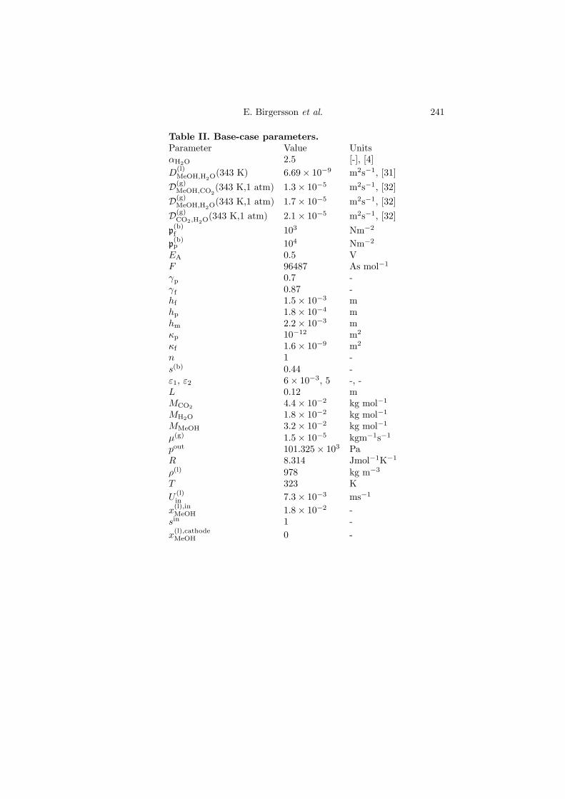
E. Birgersson et al. 241
Table II. Base-case parameters.Parameter Value UnitsαH2O 2.5 [-], [4]D(l)MeOH,H2O
(343 K) 6.69× 10⁻⁹ m2s−1, [31]D(g)MeOH,CO2
(343 K,1 atm) 1.3× 10⁻⁵ m2s−1, [32]D(g)MeOH,H2O(343 K,1 atm) 1.7× 10⁻⁵ m2s−1, [32]D(g)CO2,H2O
(343 K,1 atm) 2.1× 10⁻⁵ m2s−1, [32]p(b)f 103 Nm−2
p(b)p 104 Nm−2
EA 0.5 VF 96487 As mol−1
γp 0.7 -γf 0.87 -hf 1.5× 10⁻³ mhp 1.8× 10⁻⁴ mhm 2.2× 10⁻³ mκp 10−12 m2
κf 1.6× 10⁻⁹ m2
n 1 -s(b) 0.44 -ε1, ε2 6× 10⁻³, 5 -, -L 0.12 mMCO2
4.4× 10⁻² kg mol−1
MH2O 1.8× 10⁻² kg mol−1
MMeOH 3.2× 10⁻² kg mol−1
µ(g) 1.5× 10⁻⁵ kgm−1s−1
pout 101.325× 10³ PaR 8.314 Jmol−1K−1
ρ(l) 978 kg m−3
T 323 KU(l)in 7.3× 10⁻³ ms−1
x(l),inMeOH 1.8× 10⁻² -
sin 1 -x(l),cathodeMeOH 0 -
242 A Reduced Model for Analysis of the Anode of a DMFC
4.2. Narrow-gap approximation. Recognizing the slenderness of theanode, i.e. hf/L, hp/L¿ 1, we scale further with
X = x, Y =y
σ, U = u, V =
v
σ, U (l,g) = u(l,g), V (l,g) =
v(l,g)
σ(61)
where σ = hf/L ∼ 10−2. Neglecting terms of O(σ2) and introducing
∆ =1
Reσ2(∼ 4), Ω1 =
Λ1σ(∼ 3× 10⁻³), Ω2 =
Λ2σ(∼ 3× 10⁻⁴), (62)
yields
∂
∂X(sU) +
∂
∂Y(sV ) = 0, (63)
∂P
∂X= −µχκU, (64)
∂P
∂Y= −σ2µχκV −Gr−1σρk, (65)
∂
∂X
ÃsU
Ãλ(l)
"x(l)MeOH
x(l)CO2
#+
λ(g)
M(g)
"x(g)MeOH
x(g)CO2
#!!+
∂
∂Y
ÃsV
Ãλ(l)
"x(l)MeOH
x(l)CO2
#+
λ(g)
M(g)
"x(g)MeOH
x(g)CO2
#!!=
∂
∂Y
Ã∆sγ
32D(l)
Sc(l)∂
∂Y
"x(l)MeOH
x(l)CO2
#+∆(1− s)γ
32 ρ(g)M(g)
Sc(g)¡M(g)
¢2 ∂
∂Y
"x(g)MeOH
x(g)CO2
#!
− ∂
∂Y
Ã∆χpχ
−1κ
Sc(c)
Ã"x(l)MeOH
x(l)CO2
#− 1
M(g)
"x(g)MeOH
x(g)CO2
#!λ(l)λ(g)s
µ
∂J
∂Y
!, (66)
as Glσ ¿ 1.The corresponding boundary conditions are now given by
U = 1, x(l)MeOH = x
(l),inMeOH, s = sin at X = 0, 0 ≤ Y ≤ 1; (67)
V =∂x
(l)MeOH
∂Y=
∂s
∂Y= 0 at 0 ≤ X ≤ 1, Y = 1; (68)
∂x(l)MeOH
∂X=
∂s
∂X= 0, P (l) = 0 at X = 1, 0 ≤ Y ≤ 1; (69)
U =∂x
(l)MeOH
∂X=
∂s
∂X= 0 at X = 0, 1, −H ≤ Y ≤ 0; (70)
where H = hp/hf . At the active region (0 ≤ X ≤ 1, Y = −H),
ρV = −Ω1IΦ6− Ω2MMeOH
³x(l)MeOH − x
(l),cathodeMeOH
´x(l),inMeOH
, (71)
E. Birgersson et al. 243
and
NMeOH · eY = −Ω1I6(1 + 6αMeOH)− Ω2
³x(l)MeOH − x
(l),cathodeMeOH
´x(l),inMeOH
, (72)
NCO2 · eY =Ω1I6
. (73)
At the interface between the porous backing and the net (0 ≤ X ≤ 1, Y = 0):
s|Y=0+ = s|Y=0− , x(l)MeOH
¯Y=0+
= x(l)MeOH
¯Y=0−
, (74)
V |Y=0+ = V |Y=0− , P |Y=0+ = P |Y=0− , (75)
NMeOH|Y=0+ · eY = NMeOH|Y=0− · eY , NCO2 |Y=0+ · eY = NCO2 |Y=0− · eY .(76)
4.3. Porous backing. We proceed further by noting that V ∼ O(max(Ω1,Ω2))in Eq. 71. At sufficiently high currents (% 20 mA cm−2) Ω1 > Ω2 but the flowinduced by the methanol diffusion will dominate at lower currents, i.e. Ω2 >Ω1. To retain a general notation, we define Ω = max(Ω1,Ω2). Rescaling withΩbV = V in the porous backing, we arrive at
sbV = −IΩ1Φ6Ω
− Ω2ΩMMeOH
³x(l)MeOH − x
(l),cathodeMeOH
´x(l),inMeOH
, (77)
U = 0 +O(χ−1κ ), (78)∂P
∂Y= 0 +O(Gr−1σ), (79)
sΩbV Ãλ(l) " x(l)MeOH
x(l)CO2
#+
λ(g)
M(g)
"x(g)MeOH
x(g)CO2
#!− ∆sγ
32D(l)
Sc(l)∂
∂Y
"x(l)MeOH
x(l)CO2
#
− ∆(1− s)γ32 ρ(g)M(g)
Sc(g)¡M(g)
¢2 ∂
∂Y
"x(g)MeOH
x(g)CO2
#
+∆χpχ
−1κ
Sc(c)
Ã"x(l)MeOH
x(l)CO2
#− 1
M(g)
"x(g)MeOH
x(g)CO2
#!λ(l)λ(g)s
µ
∂J
∂Y
=
"−Ω1I/6 (1 + 6αMeOH)− Ω2
³x(l)MeOH − x
(l),cathodeMeOH
´/x
(l),inMeOH
Ω1I/6
#. (80)
Here, we have integrated the governing equations once with respect to Y , sat-isfying boundary conditions 71, 72 and 73. The transport of momentum andspecies is hence only in the normal direction of the porous backing. A similarscaling of the normal velocity was also applied for a corresponding one-phasemodel [1].

244 A Reduced Model for Analysis of the Anode of a DMFC
4.4. Net. Returning to the net, we observe that the pressure derivativein the streamwise direction, eq. 64, is balanced by the velocity term. Inaddition, the normal velocity V is O(Ω) at the interface to the porous backing(Y = 0) and O(0) as we approach the upper wall (Y = 1), hence, the governingequations in the net reduce to
∂
∂X(sU) = 0, (81)
∂P
∂X= −µU, (82)
∂P
∂Y= 0 +O(Gr−1σ), (83)
where the solution to the ODE for the streamwise velocity, Eq. 81, is given bythe inlet conditions, namely
U =sin
s, (84)
whence
sin∂
∂X
Ãλ(l)
"x(l)MeOH
x(l)CO2
#+
λ(g)
M(g)
"x(g)MeOH
x(g)CO2
#!=
∂
∂Y
Ã∆sγ
32D(l)
Sc(l)∂
∂Y
"x(l)MeOH
x(l)CO2
#+∆(1− s)γ
32 ρ(g)M(g)
Sc(g)¡M(g)
¢2 ∂
∂Y
"x(g)MeOH
x(g)CO2
#!
− ∂
∂Y
Ã∆
Sc(c)
Ã"x(l)MeOH
x(l)CO2
#− 1
M(g)
"x(g)MeOH
x(g)CO2
#!λ(l)λ(g)s
µ
∂J
∂Y
!. (85)
We have p(b)f /pref ¿ 1 and ∆p(l)/pref ¿ 1, whence we no longer need tosolve for the pressure throughout the net, since the gas density reduces toρ(g) =M(g). This assumption is reasonable, since any DMFC which requiresa pressure drop & pref , would lessen the efficiency of the cell due to the workthat has to be provided to maintain the pressure head.
4.5. Estimate of the liquid saturation. An estimate of the liquid sat-uration can be found by noticing that Sc(c) ¿ Sc(l,g), whence for the net, thetransport equation for carbon dioxide reduces, at leading order in Sc(c), to∂J/∂Y = 0, and thence ∂s/∂Y = 0, which implies that s = s (X) . Introducingthe following series expansions
s = s0 (X) + Sc(c)s1 (X,Y ) + o(Sc(c)), (86)
λ(g) = λ(g)0 + Sc(c)λ
(g)1 + o(Sc(c)), (87)
λ(l) = λ(l)0 + Sc(c)λ
(l)1 + o(Sc(c)), (88)
J = J0 + Sc(c)J1 + o(Sc(c)), (89)

E. Birgersson et al. 245
and returning to the transport equation for carbon dioxide in the net, Eq. 85,we obtain, at O(Sc(c))
sin∂
∂X
Ãλ(l)0 x
(l)CO2
+λ(g)0
M(g)x(g)CO2
!=
∂
∂Y
Ã∆s0γ
32D(l)
Sc(l)∂
∂Y
"x(l)MeOH
x(l)CO2
#
+∆(1− s0)γ
32 ρ(g)M(g)
Sc(g)¡M(g)
¢2 ∂
∂Y
"x(g)MeOH
x(g)CO2
#!
− ∂
∂Y
ÃÃ−x(g)CO2
M(g)
!λ(l)0 λ
(g)0 s0µ
dJ0ds
∂s1∂Y
!, (90)
as x(l)CO2¿ x
(g)CO2
.A useful simplification can derived by assuming the left-hand side of Eq.
90 to be independent of Y (a step justified a posteriori by examining thefunction ζ defined below by comparing with the full solution). We proceed byintegrating once with respect to Y , to obtain
sin∂
∂X
Ãλ(l)0 x
(l)CO2
+λ(g)0
M(g)x(g)CO2
!(Y − 1) = ∆s0γ
32D(l)
Sc(l)∂
∂Y
"x(l)MeOH
x(l)CO2
#
+∆(1− s0)γ
32 ρ(g)M(g)¡
M(g)¢2 ∂
∂Y
"x(g)MeOH
x(g)CO2
#−Ã−x(g)CO2
M(g)
!λ(l)0 λ
(g)0 s0µ
dJ0ds
∂s1∂Y
;
(91)
here we have applied the boundary conditions for the upper wall, Eq. 68. Theanalysis has shown that the transport is unidirectional in the porous backing,and more specifically, for our purpose, we note that NCO2 · eY is a function ofX alone, and furthermore that
NCO2· eY (X) = ΩI(X)/6
for any given position in the porous backing. At (0 ≤ X ≤ 1, Y = 0), Eqs. 91,74, 75, 76 and 80, yield
−sin ∂
∂X
Ãλ(l)x
(l)CO2
+λ(g)
M(g)x(g)CO2
!= −Ω1I(X)
6+sΩbV Ãλ(l)x(l)CO2
+λ(g)
M(g)x(g)CO2
!,
(92)and introducing sΩbV from Eq. 77, we arrive at
∂ζ
∂X=Ω1I(X)6sin
(1 +Φζ) +
Ω2MMeOH
µx(l)MeOH
¯Y=−H
− x(l),cathodeMeOH
¶sinx
(l),inMeOH
ζ, (93)
where ζ = λ(l)x(l)CO2
+ λ(g)/M(g)x(g)CO2
. This ODE for ζ replaces the transportequation for carbon dioxide in the net, provided that the capillary pressure issufficiently high to give s(X) at leading order.

246 A Reduced Model for Analysis of the Anode of a DMFC
To summarize the analysis thus far: we have found that the operatingconditions of the anode, with Ω¿ 1, leads to a decoupling of the velocity fieldin the net, where
U = sin/s+O(Ω¿ 1),
V = 0 +O(Ω¿ 1);
in addition, we only need to solve the transport equations for methanol andcarbon dioxide, and the gas density is given by ρ(g) = M(g). In the porousbacking, we arrived at
U = 0 +O(χ−1κ ¿ 1),
V = −IΩ1Φ/(6sΩ)− Ω2/(sΩ)MMeOH
³x(l)MeOH − x
(l),cathodeMeOH
´/x
(l),inMeOH
We are thus left with solving for the transport equations for methanol andcarbon dioxide, with the appropriate boundary conditions.
5. Numerics and verification
The number of unknowns to be solved are reduced by invoking the equi-librium constraints. In addition, the gradients for all mole fractions can bewritten in terms of the gradient of the liquid mole fraction of methanol. Toimprove the convergence, we treat the equilibrium conditions as independentof the gas pressure, which holds in the net, but introduces a small error in theporous backing since the capillary pressure p(b)p is not negligible compared tothe overall pressure pref .
We also have to consider the gradients of the capillary pressure for thecapillary diffusive terms in the transport equations for methanol and carbondioxide
∆χpχ−1κ
Sc(c)
Ã"x(l)MeOH
x(l)CO2
#− 1
M(g)
"x(g)MeOH
x(g)CO2
#!λ(l)λ(g)s
µ
∂J
∂s
∂s
∂Y, (94)
as s→ 1. In this limit, we see that (N.B. λ(l) ≈ 1)lims→1
λ(g) = lims→1
ε1(1− s)n+ε2 = 0, (95)
implying a vanishing diffusion coefficient. To avoid this singularity, it is advan-tageous from the numerical point of view to solve instead for the variable S,given by
S =(1− s)n+ε2+1
n+ ε2 + 1. (96)
In particular, without the above transformation, the grid density would have tobe increased significantly near the inlet to capture this increase; the variable S,on the other hand, and in particular its derivatives behaves regularly, removingthe need for an overly fine grid at the inlet, as well as improving convergence.
The reduced model is parabolic, for which a Keller Box discretizationscheme is suitable. The resulting system of non-linear equations is solved witha Newton-Raphson-based scheme in MATLAB 6. To ensure the validity of
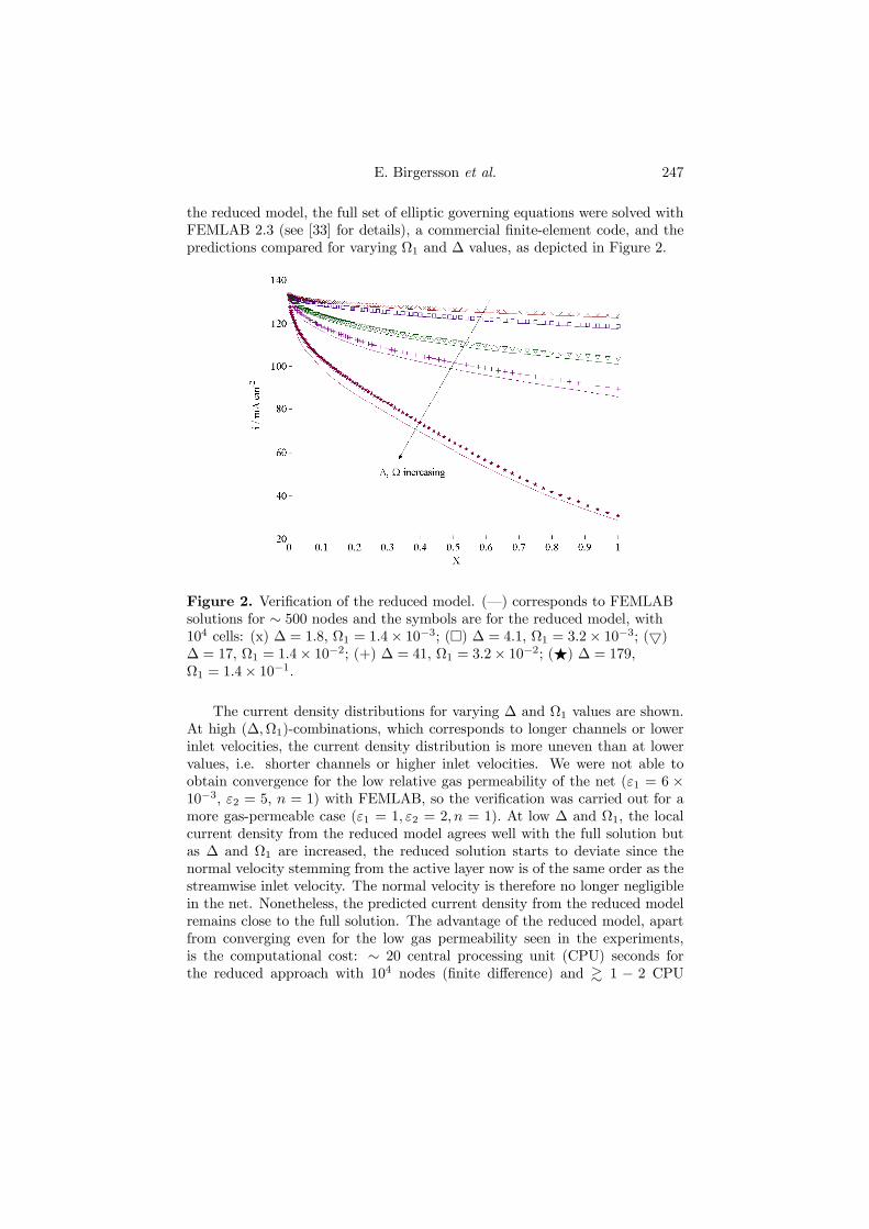
E. Birgersson et al. 247
the reduced model, the full set of elliptic governing equations were solved withFEMLAB 2.3 (see [33] for details), a commercial finite-element code, and thepredictions compared for varying Ω1 and ∆ values, as depicted in Figure 2.
Figure 2. Verification of the reduced model. (–) corresponds to FEMLABsolutions for ∼ 500 nodes and the symbols are for the reduced model, with104 cells: (x) ∆ = 1.8, Ω1 = 1.4× 10⁻³; (¤) ∆ = 4.1, Ω1 = 3.2× 10⁻³; (5)∆ = 17, Ω1 = 1.4× 10⁻²; (+) ∆ = 41, Ω1 = 3.2× 10⁻²; (F) ∆ = 179,Ω1 = 1.4× 10⁻¹.
The current density distributions for varying ∆ and Ω1 values are shown.At high (∆,Ω1)-combinations, which corresponds to longer channels or lowerinlet velocities, the current density distribution is more uneven than at lowervalues, i.e. shorter channels or higher inlet velocities. We were not able toobtain convergence for the low relative gas permeability of the net (ε1 = 6 ×10⁻³, ε2 = 5, n = 1) with FEMLAB, so the verification was carried out for amore gas-permeable case (ε1 = 1, ε2 = 2, n = 1). At low ∆ and Ω1, the localcurrent density from the reduced model agrees well with the full solution butas ∆ and Ω1 are increased, the reduced solution starts to deviate since thenormal velocity stemming from the active layer now is of the same order as thestreamwise inlet velocity. The normal velocity is therefore no longer negligiblein the net. Nonetheless, the predicted current density from the reduced modelremains close to the full solution. The advantage of the reduced model, apartfrom converging even for the low gas permeability seen in the experiments,is the computational cost: ∼ 20 central processing unit (CPU) seconds forthe reduced approach with 104 nodes (finite difference) and & 1 − 2 CPU

248 A Reduced Model for Analysis of the Anode of a DMFC
minutes for FEMLAB 2.3 with 500 nodes (finite elements) on a 2 GHz PC.Mesh-independent solutions for the reduced model were found for . 103 nodes.
6. Experimental
The experiments were run on a fuel cell with a transparent acrylic plasticendplate on the anode side (for further details, see [25]). Since it is of interestto study the DMFC at a variety of temperatures, the cell was designed to givean even temperature distribution by mounting a circuit for cooling/heatingdirectly behind the cathode, as shown in Figure 3.
Transparent end plate
End plate with heat exchanger
Meshflowfield
Five layeredMEA
Humidified H2
Fuel saturatedwith CO2
Figure 3. The principle of the visual fuel cell.
The flowfield was a gold-plated stainless steel mesh with dimensions 1.50mm, 40 mm, 130 mm in height, width and length, respectively, and having1.35x1.35 mm gaps. The porosity of the mesh was measured to be 0.87. Inaddition to the visual cell, the system comprises a peristaltic pump (WatsonMarlow), a humidifier (Fuel Cell Technologies, Inc.), a pre-heater, a fuel reser-voir, a circuit for cooling/heating water, a phase separator, pressure probesand means to measure gas- and liquid flows.
The membrane-electrode-assembly (MEA), manufactured by BCS Fuel CellsInc., has a noble metal loading of 1.6 mg/cm2 PtRu on the anode (1:1, 60%on C) and 1.6 mg/cm2 Pt on the cathode (60% on C). The thickness of theanode active layer was 14 µm, measured with SEM, and the membrane usedwas Nafion 117. The MEA has five layers, with a carbon cloth gas diffusionlayer (also referred to as porous backing) attached directly to the electrodes(also known as active layers). The MEA with a 40x120 mm2 active layer wasproduced from the same batch as the 1 cm2 MEA characterized in a separatestudy [21].
The cathode reaction in the experiments was hydrogen evolution, whichwas chosen in order to minimize the losses on the cathode and to provide arelatively stable cathode potential due to the fast hydrogen evolution kinetics.Humidified N2 (5.0) was fed to the cathode side, with a saturation temperature15 degrees above the temperature of the cell. The methanol/water fuel mixturewas preheated to the temperature of the cell and saturated with CO2. A 1Mmethanol solution was used in the experiments (pro analysi, Merck and MilliQwater).

E. Birgersson et al. 249
The measurements were run in galvanostatic mode with a current source.The noise in the experimental data is within ± 5 mV. All experimental dataare taken under steady-state conditions. At low current densities, steady statecould be reached after about 100 s, whereas up to 1000 s could be necessaryfor higher current densities.
The experimental data is not directly comparable to the modeled data asthe experimental data includes losses on the cathode due to the hydrogen evo-lution, external contact resistance, resistance through the membrane and otherinternal resistances. The external contact resistance was measured and wasfound to higher than the membrane resistance. The losses due to hydrogenevolution kinetics were neglected. The experimental data in the anode polar-ization curves was compensated for the iR-drop by fitting a term RSUM to themodel data at low potentials where methanol depletion is negligible and thusthe current density is controlled completely by the methanol oxidation kinetics.
7. Results and discussion
The analysis has shown that the flow can be described by several dimen-sionless numbers: ∆, Ω1, Ω2, H, Sc(g,l,c), Ca, Gr, Gl. In addition to these, therelative permeabilities κ(g,l)rel will have an impact on the resulting pressure dropand gas saturation throughout the anode. The absolute and relative perme-abilities can be viewed as material parameters for the net and porous backing.
7.1. Pressure drop and relative permeabilities. In order to deter-mine these for the net, the pressure drop was first measured for a pure liquidphase flow, i.e. with no current drawn from the cell, given by the lower curvein Figure 4. This case allows us to adapt the absolute permeability in the net,which we find to be 1.6 × 10⁻⁹ m2. The model overpredicts the liquid phasepressure drop, which is O(0−103) Pa, by around 30% in the intermediate rangeof 5×10⁻³-1.5×10⁻² ms−1. This deviation can be attributed to the liquid phaseflow deviating from the region of validity of Darcy’s law into a regime, where theinertial contribution becomes important. A better fit could have been obtainedby including a Forchheimer term for the liquid phase. The multiphase mixtureformulation, however, is based on the pressure drops for the phases being linearfunctions of the velocity, i.e. accounting for the surface drag from friction, butnot for form drag stemming from the solid matrix. The overall pressure drop inthe one-phase regime is still much lower than the ambient pressure, whence itscontribution to the transport of methanol and carbon dioxide is negligible, i.e.as was shown in the analysis (∆p(l)/pref ¿ 1). As soon as a current is drawnfrom the cell, carbon dioxide is created from the oxidation of methanol at theactive layer in the anode. Once the carbon dioxide pressure is sufficiently highand nucleation can occur, a gas will evolve and the pressure drop in the netincreases dramatically, even at low velocities, as is illustrated by the upper twocurves in Figure 4. This is due to increased resistance to the mixed two-phaseflow, given by the relative permeabilities κ(g,l)rel . Returning to Eq. 6, we see
that the increase in pressure head correlates directly with κ(l)rel. Based on these

250 A Reduced Model for Analysis of the Anode of a DMFC
pressure drops for coexisting liquid and gas flow and the amount of gas in thestreamwise direction, see Figure 5, the relative permeabilities were estimatedas κ(l)rel = s and κ
(g)rel = 6 × 10⁻³(1 − s)6. With these adaptions, we are able
to predict the pressure drop for the two-phase flow quite well for the velocityrange considered here.
0 0.005 0.01 0.015 0.02 0.0250
500
1000
1500
2000
2500
Uin / ms- 1
δ p(l)
/ Pa
Figure 4. Pressure drops δp(l) = p(l)(x = 0)− p(l)(x = L) from experimentsand predictions from the reduced model. Experimental values: (H) no current,(¥) 68 mA cm−2 and (•) 79 mA cm−2. Model predictions: (–) no current,(− ·−) 68 mA cm−2, and (−−) 79 mA cm−2. The temperature is 45oC.
7.2. Gas saturation in the net. The relative gas permeability mightappear surprisingly low, but the net that was employed proved to have a highresistance to the gas flow, trapping gas bubbles in its gaps, and giving rise toa large gas saturation, as illustrated in Figure 5. Here, several features areapparent; foremost are the large fluctuations in the measured gas saturationin the streamwise direction, especially for the case of the lower velocity. Theseare a consequence of local variations in gas formation activity at the interfacebetween the porous backing and the net as well, as the small number of gapsin the spanwise direction at any given streamwise position. A more detaileddiscussion of these fluctuations can be found in [25]. The pressure drop for thetwo-phase mixture is O(103) Pa, which is still small compared to that underambient conditions. Computationally, the large amount of gas, even close tothe inlet, causes problems, since the gas saturation variable, s(g), which iszero at the inlet, has to rapidly increase to around 0.7. To accommodate thisrapid change, we introduced the variable S, as described earlier. Note that
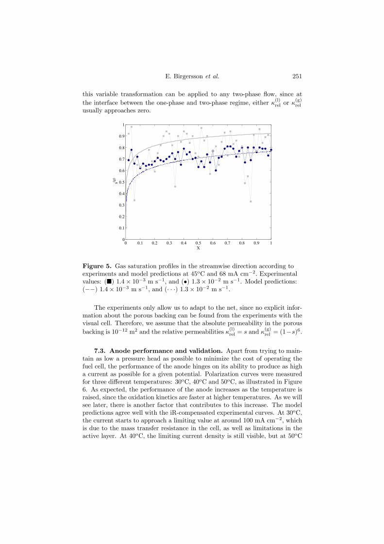
E. Birgersson et al. 251
this variable transformation can be applied to any two-phase flow, since atthe interface between the one-phase and two-phase regime, either κ(l)rel or κ
(g)rel
usually approaches zero.
0 0.1 0.2 0.3 0.4 0.5 0.6 0.7 0.8 0.9 10
0.1
0.2
0.3
0.4
0.5
0.6
0.7
0.8
0.9
1
X
s(g)
Figure 5. Gas saturation profiles in the streamwise direction according toexperiments and model predictions at 45oC and 68 mA cm−2. Experimentalvalues: (¥) 1.4× 10⁻³ m s−1, and (•) 1.3× 10⁻² m s−1. Model predictions:(−−) 1.4× 10⁻³ m s−1, and (· · ·) 1.3× 10⁻² m s−1.
The experiments only allow us to adapt to the net, since no explicit infor-mation about the porous backing can be found from the experiments with thevisual cell. Therefore, we assume that the absolute permeability in the porousbacking is 10−12 m2 and the relative permeabilities κ(l)rel = s and κ(g)rel = (1−s)6.
7.3. Anode performance and validation. Apart from trying to main-tain as low a pressure head as possible to minimize the cost of operating thefuel cell, the performance of the anode hinges on its ability to produce as higha current as possible for a given potential. Polarization curves were measuredfor three different temperatures: 30oC, 40oC and 50oC, as illustrated in Figure6. As expected, the performance of the anode increases as the temperature israised, since the oxidation kinetics are faster at higher temperatures. As we willsee later, there is another factor that contributes to this increase. The modelpredictions agree well with the iR-compensated experimental curves. At 30oC,the current starts to approach a limiting value at around 100 mA cm−2, whichis due to the mass transfer resistance in the cell, as well as limitations in theactive layer. At 40oC, the limiting current density is still visible, but at 50oC

252 A Reduced Model for Analysis of the Anode of a DMFC
we are still far from reaching such a limit, even though the current that can bedrawn from the cell is significantly higher than at lower temperatures. Thesepolarization curves represent global averages of the current obtained along theactive layer in the streamwise direction, and as we saw in Figure 2, the localcurrent density can decrease considerably.
0 20 40 60 80 100 120 140 160 180 2000.25
0.3
0.35
0.4
0.45
0.5
0.55
0.6
0.65
0.7
i / mA cm - 2
pote
ntia
l / V
Temperature increasing
30°C
50°C
40°C
Figure 6. Polarization curves for experiments and model predictions. Theinlet velocity U in = 7.3× 10⁻³ m s−1and the methanol concentration is 1 M.Experimental values: (•) 30oC , (H) 40oC, and (¥) 50oC. Model predictions:(− ·−) 30oC, (−−) 40oC and (–) 50oC.
This decrease of current along the streamwise direction stems frommethanoldepletion, as depicted in Figures 7a and 7b, where the predicted mole fractionof methanol in the liquid and gas phase, respectively, are shown. We see thatthe mole fraction of methanol is somewhat higher in the gas phase than in theliquid phase, and that gradients exist in both phases towards the active layerand the outlet. The question that arises is whether the gas phase transport ofmethanol affects the overall transport of methanol to the active layer and, ifso, to what extent. The answer is in the affirmative, with the explanation lyingin the magnitude of the dimensionless ratios: ∆/Sc(l) ∼ 3× 10⁻² for the liquidphase transport and ∆/Sc(g) ∼ 5×10⁻² for the gas phase; these are of the sameorder of magnitude, whence both phases will contribute more or less equallyto the transport of methanol, provided that the gas- and liquid mole fractionsare of the same order of magnitude and that a liquid and gas phase exist. Thegradients for the methanol mole fractions are clearly visible, whereas for thecarbon dioxide, the changes in mole fractions are negligible in both liquid and

E. Birgersson et al. 253
gas phases, as can be inferred from Figures 7c and 7d - a contrast to the ex-treme gradients predicted by the one-phase model [1]. Furthermore, most ofthe resistance to species transfer in the net lies in a boundary layer adjacentto the porous backing, since ∆/Sc(l), ∆/Sc(g) ¿ 1 for the base case.
0 0.2 0.4 0.6 0.8 1-0.1
0
0.1
0.2
0.3
0.4
0.5
0.6
0.7
0.8
0.9
X
Y
0.0130.0140.0140.015
0.0150.0160.0160.017
0.017
a) xMeOH(l)
Figure 7a. Methanol mole fraction in the liquid for the base case.
0 0.2 0.4 0.6 0.8 1-0.1
0
0.1
0.2
0.3
0.4
0.5
0.6
0.7
0.8
0.9
X
Y
0.0140.0150.0160.016
0.017
0.0170.018
0.0180.019
0.019
b) xMeOH(g)
Figure 7b. Methanol mole fraction in the gas for the base case.
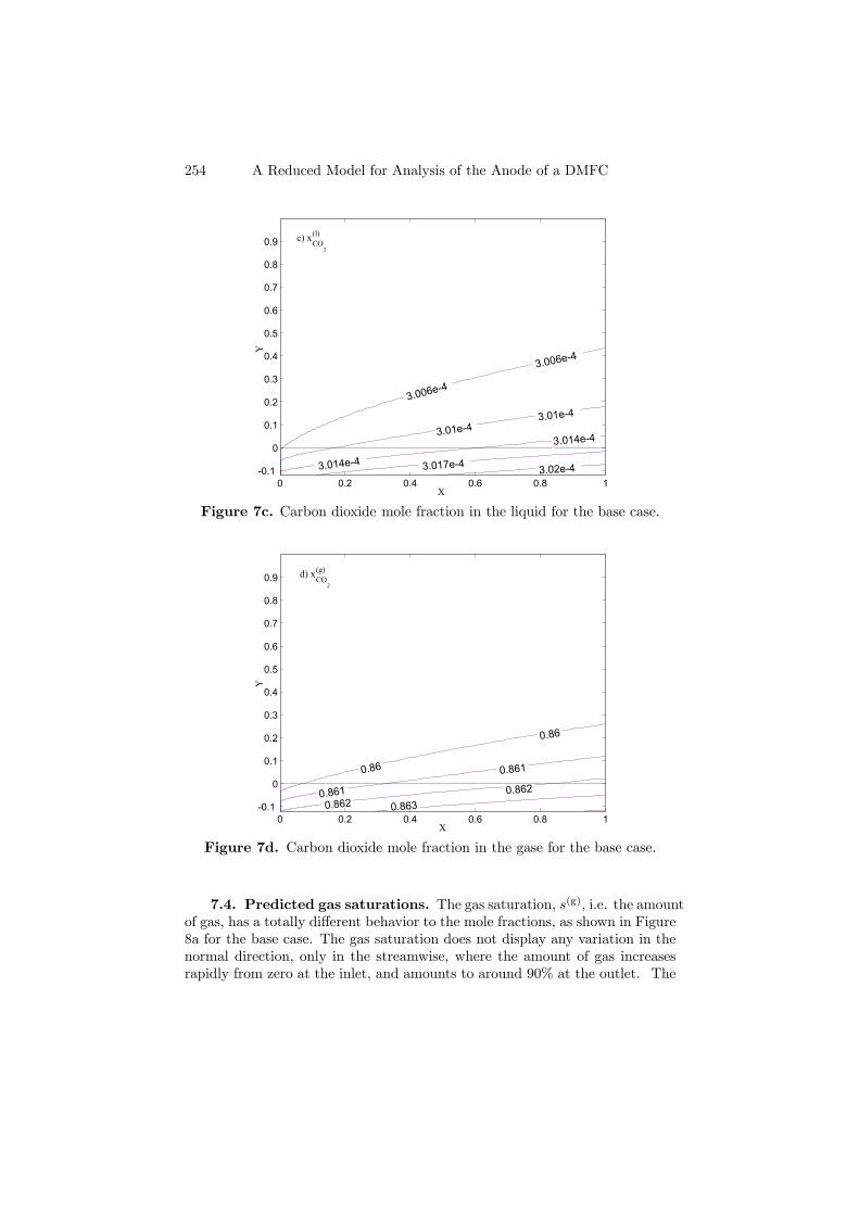
254 A Reduced Model for Analysis of the Anode of a DMFC
0 0.2 0.4 0.6 0.8 1-0.1
0
0.1
0.2
0.3
0.4
0.5
0.6
0.7
0.8
0.9
X
Y
3.006e-4
3.01e-43.014e-4
3.017e-4 3.02e-4
3.006e-4
3.01e-4
3.014e-4
c) xCO
2
(l)
Figure 7c. Carbon dioxide mole fraction in the liquid for the base case.
0 0.2 0.4 0.6 0.8 1-0.1
0
0.1
0.2
0.3
0.4
0.5
0.6
0.7
0.8
0.9
X
Y
0.86
0.86
0.861
0.861
0.8620.862
0.863
d) xCO
2
(g)
Figure 7d. Carbon dioxide mole fraction in the gase for the base case.
7.4. Predicted gas saturations. The gas saturation, s(g), i.e. the amountof gas, has a totally different behavior to the mole fractions, as shown in Figure8a for the base case. The gas saturation does not display any variation in thenormal direction, only in the streamwise, where the amount of gas increasesrapidly from zero at the inlet, and amounts to around 90% at the outlet. The
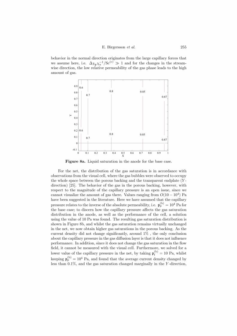
E. Birgersson et al. 255
behavior in the normal direction originates from the large capillary forces thatwe assume here, i.e. ∆χpχ
−1κ /Sc(c) À 1 and for the changes in the stream-
wise direction, the low relative permeability of the gas phase leads to the highamount of gas.
0 0.1 0.2 0.3 0.4 0.5 0.6 0.7 0.8 0.9 1-0.1
0
0.1
0.2
0.3
0.4
0.5
0.6
0.7
0.8
0.9
X
Y
0.6
0.6
0.7
0.7
0.8
0.8
0.85
0.85
0.87
0.87
Figure 8a. Liquid saturation in the anode for the base case.
For the net, the distribution of the gas saturation is in accordance withobservations from the visual cell, where the gas bubbles were observed to occupythe whole space between the porous backing and the transparent endplate (Y -direction) [25]. The behavior of the gas in the porous backing, however, withrespect to the magnitude of the capillary pressure is an open issue, since wecannot visualize the amount of gas there. Values ranging from O(10− 104) Pahave been suggested in the literature. Here we have assumed that the capillarypressure relates to the inverse of the absolute permeability, i.e. p(b)p = 104 Pa forthe base case; to discern how the capillary pressure affects the gas saturationdistribution in the anode, as well as the performance of the cell, a solutionusing the value of 10 Pa was found. The resulting gas saturation distribution isshown in Figure 8b, and whilst the gas saturation remains virtually unchangedin the net, we now obtain higher gas saturations in the porous backing. As thecurrent density did not change significantly, around 1% , the only conclusionabout the capillary pressure in the gas diffusion layer is that it does not influenceperformance. In addition, since it does not change the gas saturation in the flowfield, it cannot be measured with the visual cell. Furthermore, we solved for alower value of the capillary pressure in the net, by taking p(b)f = 10 Pa, whilst
keeping p(b)p = 104 Pa, and found that the average current density changed byless than 0.1%, and the gas saturation changed marginally in the Y -direction,

256 A Reduced Model for Analysis of the Anode of a DMFC
but gave the same overall increase in the X-direction and deviated by less than1% at the outlet.
0 0.1 0.2 0.3 0.4 0.5 0.6 0.7 0.8 0.9 1-0.1
0
0.1
0.2
0.3
0.4
0.5
0.6
0.7
0.8
0.9
X
Y
0.6
0.6
0.7
0.7
0.8
0.8
0.85
0.85
0.87
0.87
0.87
0.89
Figure 8b. Liquid saturation in the anode for the base case with p(b)p = 10Nm−2.
Can we explain the reason for the capillary pressure in the net havingvirtually no impact on the resulting flow? The answer is again in the affirmative:returning to the analysis, Eq. 85 in particular, we see that the capillary pressurein the streamwise direction for the slender net was removed in the narrow-gapapproximation. Should the capillary pressure, however, be even larger than wetake it to be in the net, this approximation might no longer hold, and capillarypressure-driven flow in the streamwise direction has to be retained, even forthe slender case.
7.5. Methanol concentration dependence. So far, the concentrationof methanol has been 1 M, but larger concentrations, as well as smaller, arefeasible, as illustrated in Figure 9. Intuitively, we expect the local current den-sity to increase as the concentration is raised, but also for the loss of methanol,given by Ω2, to increase. Since Ω2(4 M) ≈ Ω2(1 M)/4, the loss of methanolthrough the membrane does not increase substantially at the highest molar con-centration that we consider here, 4 M. The local current density does indeedincrease as more methanol is added to the fuel, and we note that the largestdeviations from [i] are obtained at the lowest concentrations. We recall that [i]is the current density for the inlet concentration of methanol and as such givesthe ‘ideal’ current density for the anode, since no mass transfer resistances ordepletion of methanol are considered. For the highest concentration, 4 M, the
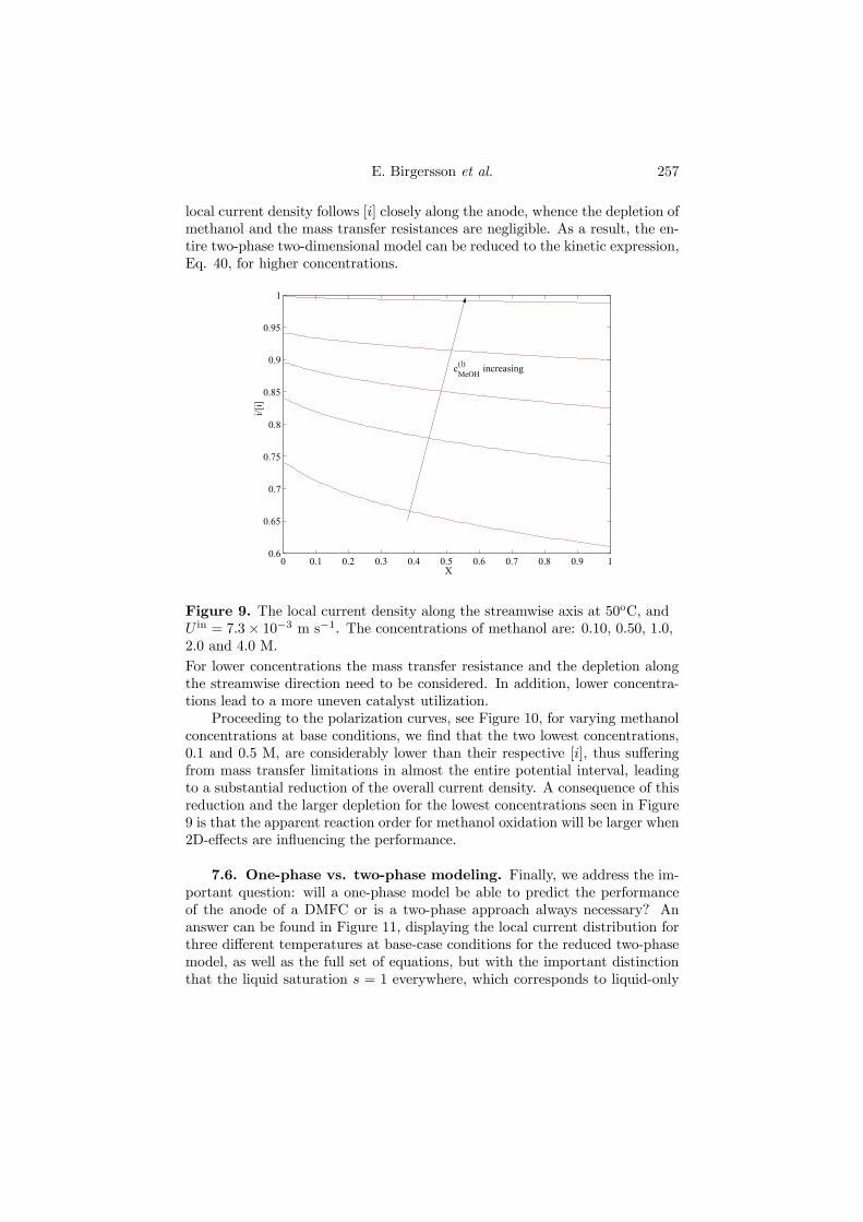
E. Birgersson et al. 257
local current density follows [i] closely along the anode, whence the depletion ofmethanol and the mass transfer resistances are negligible. As a result, the en-tire two-phase two-dimensional model can be reduced to the kinetic expression,Eq. 40, for higher concentrations.
0 0.1 0.2 0.3 0.4 0.5 0.6 0.7 0.8 0.9 10.6
0.65
0.7
0.75
0.8
0.85
0.9
0.95
1
i/[i]
X
cMeOH(l) increasing
Figure 9. The local current density along the streamwise axis at 50oC, andU in = 7.3× 10⁻³ m s−1. The concentrations of methanol are: 0.10, 0.50, 1.0,2.0 and 4.0 M.For lower concentrations the mass transfer resistance and the depletion alongthe streamwise direction need to be considered. In addition, lower concentra-tions lead to a more uneven catalyst utilization.
Proceeding to the polarization curves, see Figure 10, for varying methanolconcentrations at base conditions, we find that the two lowest concentrations,0.1 and 0.5 M, are considerably lower than their respective [i], thus sufferingfrom mass transfer limitations in almost the entire potential interval, leadingto a substantial reduction of the overall current density. A consequence of thisreduction and the larger depletion for the lowest concentrations seen in Figure9 is that the apparent reaction order for methanol oxidation will be larger when2D-effects are influencing the performance.
7.6. One-phase vs. two-phase modeling. Finally, we address the im-portant question: will a one-phase model be able to predict the performanceof the anode of a DMFC or is a two-phase approach always necessary? Ananswer can be found in Figure 11, displaying the local current distribution forthree different temperatures at base-case conditions for the reduced two-phasemodel, as well as the full set of equations, but with the important distinctionthat the liquid saturation s = 1 everywhere, which corresponds to liquid-only

258 A Reduced Model for Analysis of the Anode of a DMFC
flow. At 30oC, the local current density predicted by the liquid phase modelfollows the reduced two-phase model closely, but deviates severely at 50oC and70oC.
0 20 40 60 80 100 120 140 160 180 2000.25
0.3
0.35
0.4
0.45
0.5
0.55
0.6
0.65
0.7
i / mA cm - 2
pote
ntia
l / V
cMeOH(l) increasing
Figure 10. Polarization curves as predicted by the model. Temperature is50oC and the flow rate 0.0073 m s−1. The concentrations c(l)MeOH of methanolare: 0.10, 0.50, 1.0, 2.0 and 4.0 M. For comparison, the current density scale[i] for the kinetic expression is shown for 0.10 and 0.50 M (· · ·).
It appears as if the one-phase model thus is able to predict the currentdensity accurately for low temperatures, here 30oC, but fails as the temperatureis increased. The answer to the question posed above is thence: yes, a one-phasemodel might be employed at low temperatures, and no for higher temperatures.The cause can be found in the gas phase, where the mole fraction of methanolamounts to ∼ 7×10⁻³ at 30oC and increases to ∼ 5×10⁻² at 70oC, i.e. almostten times as high. For low temperatures it might thus possible to predict theperformance via a one-phase approach, which can reduce the computationalcost significantly, as was shown by Birgersson et al. [1]. In addition, contraryto common belief that carbon dioxide hinders methanol mass transfer, thetwo-phase model predicts better performance, which can be attributed to themethanol in the gas phase contributing to the transport of methanol to theactive layer, where it is oxidized.
Considering the improved mass transfer in the gas phase it would be easyto conclude that a high gas saturation always improves performance. There is,however, always the risk of local methanol depletion in a real system, whichwe observed whilst running the visual cell at low flow rates. Bubbles were

E. Birgersson et al. 259
entrapped for long periods of time, with local methanol depletion as a result,lowering performance. Based on the knowledge acquired from the model andfrom practical experiments with the visual cell, it is possible to suggest theproperties of an ideal flow field for the anode of a DMFC so as to minimizemass transfer resistances: the flow field should retain the bubbles to keep thegas saturation high, whilst simultaneously ensuring that the entrapped gasremains in contact with "fresh" liquid fuel flowing past.
Figure 11. Current density distributions i/[i] for varying temperatures: (–)corresponds to predictions with the FEMLAB code, without the gas phaseand (−−) are predictions from the reduced two-phase model.
8. Conclusions
A two-phase model for mass, momentum and species transport in the an-ode of a DMFC has been considered. The governing equations and boundaryconditions were nondimensionalised, and a reduced model was then derived,using elementary asymptotic techniques, for the case where the anode geome-try is slender and a net-type flow field is used. The reduced model was verifiedand subsequently validated against pressure drop, gas saturation and polariza-tion curves at different temperatures measured in a DMFC equipped with atransparent end plate at the anode.
The pressure drop increases significantly when a current is drawn for thenet-type flow distributor. The reason for this drastic increase is the high gassaturation in the mesh, measured with the visual cell to be typically & 70%.There is a sharp increase in the gas saturation at the inlet, after which the

260 A Reduced Model for Analysis of the Anode of a DMFC
increase is more moderate. The model predicts that there is no gas saturationgradient in the normal direction. Lowering the capillary pressure in the gasdiffusion layer to 10 Pa in the model resulted in gas saturation gradients in theporous backing, whilst the performance was unaffected.
For the highest concentration of methanol studied, 4 M, the local currentdensity stays close to the current density scale [i], based on the inlet methanolconcentration. At such high methanol concentrations, the anode model canbe reduced to just computing [i], which entails virtually no computationalcost. At low temperatures (¹30 oC), a liquid-phase model can be sufficient forpredicting the anode performance, which allows for a considerable reduction incomputational cost. At higher temperatures the predictions from the liquid-phase model differ substantially from the two-phase approach.
The presence of a gas phase was found to improve the mass transferof methanol, especially at higher temperatures, when the mole fraction ofmethanol in the gas phase is also higher.
The characteristics of an ‘ideal’ flow field for the anode of a DMFC isdiscussed. The flow field should retain the bubbles to keep the gas saturationhigh, but it should make sure that the entrapped gas is in contact with "fresh"liquid fuel flowing past the entrapped bubbles.
Acknowledgements
Financial support from the Swedish Foundation for Strategic Environmen-tal Research, MISTRA, and from the Swedish National Energy Administrationis gratefully acknowledged. The work was done within the framework of theJungner Center. J. Nordlund gratefully acknowledges a scholarship from theErnst Johnson foundation.
E. Birgersson et al. 261
Appendix A
Mixture variables
Dimensional mixture quantities.- The mixture variables are defined as
ρ = ρ(l)s+ ρ(g)(1− s), (A.1)
ρk = λ(l)ρ(l) + λ(g)ρ(g), (A.2)
ρv = ρ(l)v(l) + ρ(g)v(g), (A.3)
µ =ρ(l)s+ ρ(g)(1− s)
ρ(l)κ(l)rel/µ
(l) + ρ(g)κ(g)rel /µ
(g), (A.4)
λ(l) =ρ(l)κ
(l)rel/µ
(l)
ρ(l)κ(l)rel/µ
(l) + ρ(g)κ(g)rel /µ
(g), (A.5)
λ(g) = 1− λ(l). (A.6)
The superficial phase velocities of the liquid and gaseous phase can be foundfrom the relations
ρ(l)v(l) =λ(l)λ(g)κρ
µ
³∇p(c) +
³ρ(l) − ρ(g)
´g´+ λ(l)ρv, (A.7)
ρ(g)v(g) = −λ(l)λ(g)κρ
µ
³∇p(c) +
³ρ(l) − ρ(g)
´g´+ λ(g)ρv. (A.8)
Non-dimensional mixture quantities.- The mixture properties are now
ρ = s, (A.9)
ρk = λ(l), (A.10)
sv = v(l) +Θρ(g)v(g), (A.11)
µ =s
κ(l)rel + Ξρ
(g)κ(g)rel
, (A.12)
λ(l) =κ(l)rel
κ(l)rel + Ξρ
(g)κ(g)rel
, (A.13)
λ(g) =Ξρ(g)κ
(g)rel
κ(l)rel + Ξρ
(g)κ(g)rel
. (A.14)
Here, Θ =£ρ(g)
¤/ρ(l) ¿ 1 and Ξ = [ρ(g)]µ(l)/(µ(g)ρ(l)).

262 A Reduced Model for Analysis of the Anode of a DMFC
The phase velocities can be found from
U (l) = Ca−1χpχ−1κ
λ(l)λ(g)s
µ
∂J
∂X+ λ(l)sU, (A.15)
V (l) = Ca−1χpχ−1κ
λ(l)λ(g)s
µσ2
µ∂J
∂Y−Glσ
¶+ λ(l)sV, (A.16)
Θρ(g)U (g) = Ca−1χpχ−1κ
λ(l)λ(g)s
µ
∂J
∂X+ λ(g)sU (A.17)
Θρ(g)V (g) = Ca−1χpχ−1κ
λ(l)λ(g)s
µσ2
µ∂J
∂Y−Glσ
¶+ λ(g)sV. (A.18)
E. Birgersson et al. 263
Appendix B
Constitutive equations for the ternary component vapor-liquid equilibrium
The fluid will be a three-component mixture of water, methanol and carbondioxide. It is therefore not possible to find all necessary data directly in theliterature, whence we are required to introduce a few minor assumptions:
(1) x(l)CO2
¿ x(l)MeOH, x
(l)H2O
.(2) The dissolved carbon dioxide does not influence the activity coeffi-
cients for methanol and water.(3) The pressure is low (i.e. not more than a few bars).(4) The Henry constant for carbon dioxide is taken as the Henry constant
in pure water; i.e. the influence of methanol is neglected.(5) The vapor phase and the liquid phase are always in equilibrium.
To deduce the compositions of the vapor- and liquid phase we use Gibbs phaserule [34]:
Var = Co− Ph + 2, (B.1)
where Var is the number of intensive variables that can be changed indepen-dently without disturbing the number of phases in equilibrium, Co is the num-ber of components and Ph is the number of phases in equilibrium. Consideringthe two-phase case with the carbon dioxide-methanol-water mixture, the num-ber of intensive variables that can be changed independently without disturbingthe number of phases in equilibrium is 3. The practical use of this is that ifwe specify the intensive variables temperature and pressure at a given point,the composition of both the liquid- and the vapor phases can be calculatedif we know the concentration of any one component in either phase. Here,we have decided to use the liquid molar fraction of methanol to calculate thecomposition in the liquid and the vapor phases.
Using assumptions 1 - 3 above, the equilibrium vapor pressures of methanoland water can be calculated using the Wilson equation with the Wilson con-stants taken from experimental investigations in literature. Using Wilson con-stants from the Vapor-Liquid Equilibrium Data Collection [35] and the corre-sponding Wilson equations, Eqs. 97-B.6, the activity coefficients for methanoland water can be calculated. The molar volume for methanol is derived bytemperature-correcting the molar volume at its boiling point by the Yamadaand Gunn extension of Rackett’s equation [36]. Antoine’s equation and con-stants are taken from [36] to derive the vapor pressures for the pure species.The activity coefficients were calculated and plotted in Figure A1 at 298, 323,338 and 373 K.
AMeOH,H2O =MH2O
MMeOHexp
µ−kMeOH,H2O
681.6
¶, (B.2)
AH2O,MeOH =MMeOH
MH2Oexp
µ−kH2O,MeOH
681.6
¶, (B.3)

264 A Reduced Model for Analysis of the Anode of a DMFC
ln (γMeOH) = − ln³x(l)MeOH +AMeOH,H2Ox
(l)H2O
´+ x
(l)H2O
ÃAMeOH,H2O
x(l)MeOH +AMeOH,H2Ox
(l)H2O
− AH2O,MeOH
A2,MeOHx(l)MeOH + x
(l)H2O
!, (B.4)
ln¡γH2O
¢= − ln
³x(l)H2O
+AH2O,MeOHx(l)MeOH
´− x
(l)MeOH
ÃAMeOH,H2O
x(l)MeOH +AMeOH,H2Ox
(l)H2O
− AH2O,MeOH
AH2O,MeOHx(l)MeOH + x
(l)H2O
!, (B.5)
γi =x(g)i p(g)
x(l)i pvapi
; (B.6)
here, Aij are Wilson coefficients, γi are the activity coefficients of species i,M is the molar volume, kij are the Wilson parameter values at the specifictemperature, x(l)i and x
(g)i are the mole fractions in the liquid phase and the
gas phase, respectively. p(g) is the total gas pressure in the binary system andpvapi is the vapor pressure of the pure species i.
Table III. Data for equilibrium conditions.Parameter Value Units
kMeOH,H2O −59.6971 [-], [35]kH2O,MeOH 562.0507 [-], [35]MMeOH 43.1× 10⁻⁶ m3 mol−1
MH2O 18.4× 10⁻⁶ m3 mol−1
pvapH2O 105.11564−1687.537
T−273+230.17 × 101.325× 103 Nm−2, [36]pvapH2O 105.20277−
1580.08T−273+239.500 × 101.325× 103 Nm−2, [36]
k1, k2, k3 2.76, -74.8, -0.0140, -, -, K−1
k4, k5, k6 -0.578, 0.00406, 6.68 -, K−1,-k7, k8, k9 0.0108, 0.00621, 9.39 -, K−1,-k10, k11,k12, k13 1.00, 0.583, 0.00333, 4.77 -, -, K−1,-
As temperature dependance is not a part of the Wilson scheme, empiricalfunctions were fitted to the activity coefficients of methanol and water, result-ing in Eqs. B.7-B.8, which give the activity coefficients as a function of themethanol molar fraction in the liquid and the temperature. The adapted con-stants ki are given in Table III and the activity coefficient functions are plottedin Figure A1.
γadaptedMeOH (x(l)MeOH, T ) = k1+k2 exp(k3T )+k4(T k5)
k6x(l)MeOH+k7(T k8)
k9³x(l)MeOH
´2,
(B.7)
γadaptedH2O(x(l)MeOH, T ) = k10 + k11(T k12)
k13³x(l)MeOH
´2. (B.8)
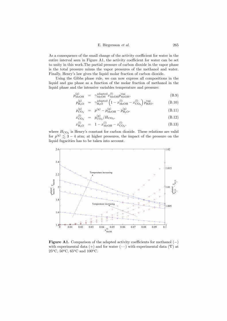
E. Birgersson et al. 265
As a consequence of the small change of the activity coefficient for water in theentire interval seen in Figure A1, the activity coefficient for water can be setto unity in this work.The partial pressure of carbon dioxide in the vapor phaseis the total pressure minus the vapor pressures of the methanol and water.Finally, Henry’s law gives the liquid molar fraction of carbon dioxide.
Using the Gibbs phase rule, we can now express all compositions in theliquid and gas phase as a function of the molar fraction of methanol in theliquid phase and the intensive variables temperature and pressure:
p(g)MeOH = γadaptedMeOH x
(l)MeOHp
vapMeOH, (B.9)
p(g)H2O
= γadaptedH2O
³1− x
(l)MeOH − x
(l)CO2
´pvapH2O, (B.10)
p(g)CO2
= p(g) − p(g)MeOH − p
(g)H2O
, (B.11)
x(l)CO2
= p(g)CO2
/HCO2 , (B.12)
x(l)H2O
= 1− x(l)MeOH − x
(l)CO2
, (B.13)
where HCO2 is Henry’s constant for carbon dioxide. These relations are validfor p(g) . 3 − 4 atm; at higher pressures, the impact of the pressure on theliquid fugacities has to be taken into account.
0 0.01 0.02 0.03 0.04 0.05 0.06 0.07 0.08 0.09 0.11.4
1.6
1.8
2
2.2
2.4
2.6
xMeOH(l)
γ MeO
Had
apte
d , γM
eOH
γ H2O
adap
ted , γ
H2O
1
1.005
1.01
1.015
1.02
Temperature increasing
Temperature increasing
Figure A1. Comparison of the adapted activity coefficients for methanol (−)with experimental data (+) and for water (· · ·) with experimental data (∇) at25oC, 50oC, 65oC and 100oC.

266 A Reduced Model for Analysis of the Anode of a DMFC
Now, recognizing HCO2 À 1, we obtain
x(g)MeOH
³p(g), T, x
(l)MeOH
´=
γadaptedMeOH x(l)MeOHp
vapMeOH
p(g), (B.14)
x(g)CO2
³p(g), T, x
(l)MeOH
´= 1−
γadaptedH2O
³1− x
(l)MeOH
´pvapH2O
p(g)
− γadaptedMeOH x(l)MeOHp
vapMeOH
p(g), (B.15)
x(l)CO2
³p(g), T, x
(l)MeOH
´=
1
HCO2
³p(g) − γadaptedMeOH x
(l)MeOHp
vapMeOH)
−γadaptedH2O
³1− x
(l)MeOH
´pvapH2O
´. (B.16)
E. Birgersson et al. 267
List of symbols
Ai,j wilson parametersci molar concentration of species i, mol m−3
ci parameters for the electrokineticsCa = µ(l)U inL/(p
(b)f κf) capillary number
Co number of componentsDij diffusion coefficients, m2 s−1
D(m)MeOH methanol diffusion in the membrane, m2s−1
Di,j binary diffusion coefficients for a pair (i,j), m2s−1
ex, ey, eX, eY, coordinate vectorsEA electrode potential of anode vs DHE, VEA potential for the electrokinetics, VF Faraday’s constant, A s mol−1
g, g gravity vector, scalar, ms−2
Gl = ρ(l)gL/p(b)f gravillary number
Gr = µ(l)U in/(ρ(l)gκf) gravitary numberh height, mH = hp/hf dimensionless height of porous backingHCO2 Henry’s law coefficient, Nm−2
i current density, Am−2
ilim limiting current density, Am−2
I dimensionless current densityJ Leverett functionkij Wilson parameterski parameters for the equilibrium conditionsL length of anode, mM mean molecular mass, kg mol−1
Mi molar mass of species i, kg mol−1
M(k), hMi(k) diffusion tensor of phase k, kg mol−1m2s−1
M, Mi dimensionless mole massMi mole volume of species i, m3 mol−1
n parameter for relative permeabilitiesNi total molar flux of species i, mol m−2s−1
p pressure, PaP dimensionless pressurep(b) breakthrough pressurePh number of phasesR gas constant, J mol−1 K−1
Re = ρ(l)U inL/µ(l) Reynolds numbers saturationS transformed liquid saturation
Sc(c) =¡µ(l)¢2/(κfρ
(l)p(b)f ) capillary Schmidt number
Sc(g) = µ(l)/(£ρ(g)
¤ £D(g)
¤) gas phase Schmidt number
Sc(l) = µ(l)/(ρ(l)£D(l)
¤) liquid phase Schmidt number
268 A Reduced Model for Analysis of the Anode of a DMFC
T anode temperature, Ku, v, v, U in velocities, m s−1
U, V, bV dimensionless velocitiesVar number of intensive variablesV volume, m3
xi mole fraction of species ix, y coordinates, mex, ey,X, Y dimensionless coordinates
Greekα coefficient for electroosmosisαA Tafel slopeγ porosityγi activity coefficientδp(l) = p(l)(x = 0)− p(l)(x = L) pressure drop, Nm−2
∆ = 1/(Reσ2) dimensionless number∆p(k) scale for pressure dropε1, ε2 parameters for rel. permeabilitiesΘ =
£ρ(g)
¤/ρ(l) dimensionless parameter
κ permeability, m2
λ mobilityΛ1 = [i][M ]/(ρ
(l)U inF ), dimensionless numberΛ2 = D
(m)MeOHx
(l),inMeOH/(U
inhm) dimensionless numberµ dynamic viscosity, kg m−1 s−1
Ξ = [ρ(g)]µ(l)/(µ(g)ρ(l)) dimensionless parameterρ density, kg m−3
σ = hf/L dimensionless numberζ = λ(l)x
(l)CO2
+ λ(g)/M(g)x(g)CO2
variable for reduced ODEτ surface tension, Nm−1
φ scalar, vector, general tensorχp = (1 net, p
(b)p /p
(b)f porous backing) dimensionless number
χκ = (1 net, κ(b)f /κ
(b)p porous backing) dimensionless number
Φ = ((1 + 6αH2O)MH2O
+(1 + 6αMeOH)MMeOH −MCO2) dimensionless numberΩ1 = Λ1/σ,Ω2 = Λ2/σ,Ω = max(Ω1,Ω2) dimensionless numbers

E. Birgersson et al. 269
Subscripts0 reference0,1 index for series expansionCO2 carbon dioxidef flow field (net)H2O wateri species ik kinematic mixturem membraneMeOH methanolp porous backingrel relative
Superscriptsadapted adapted(b) breakthrough(c) capillarycathode cathode(g) gas phasein inlet(k) phase k(l) liquid phase(m) membraneref referencevap vapor

Bibliography
[1] E. Birgersson, J. Nordlund, H. Ekström, M. Vynnycky, and G. Lindbergh, J. Elec-trochem. Soc., 150, A1368 (2003).
[2] K. Scott, W. Taama and J. Cruickshank, J. Power Sources, 65, 159 (1997).[3] K. Scott, W. Taama and J. Cruickshank, J. Appl. Electrochem., 28, 289 (1998).[4] S.F. Baxter, V.S. Battaglia, and R.E. White, J. Electrochem. Soc., 146, 437 (1999).[5] A.A. Kulikovsky, J. Divisek and A.A. Kornyshev, J. Electrochem. Soc., 147, 953 (2000).[6] H. Dohle, J. Divisek and R. Jung, J. Power Sources, 86, 469 (2000).[7] K. Scott, P. Argyropoulos and K. Sundmacher, J. Electroanal. Chem., 477, 97 (1999).[8] A.A. Kulikovsky, J. Appl. Electrochem., 30, 1005 (2000).[9] P.S. Kauranen, Acta Polytechnica Scandinavica, 237, 1 (1996).[10] K. Sundmacher, T. Schultz, S. Zhou, K. Scott, M. Ginkel and E.D. Gilles, Chem. Eng.
Sci., 56, 333 (2001).[11] S. Zhou, T. Schultz, M. Peglow and K. Sundmacher, Phys. Chem. Chem. Phys., 3, 347
(2001).[12] A.A. Kulikovsky, Electrochem. Comm., 3, 460 (2001).[13] A.A. Kulikovsky, Electrochem. Comm., 3, 572 (2001).[14] J. Nordlund, G. Lindbergh, J. Electrochem. Soc., 149, A1107 (2002).[15] J.P. Meyers, J. Newman, J. Electrochem. Soc., 149, A710 (2002).[16] J.P. Meyers, J. Newman, J. Electrochem. Soc., 149, A718 (2002).[17] J.P. Meyers, J. Newman, J. Electrochem. Soc., 149, A729 (2002).[18] Z.H. Wang and C.Y. Wang, J. Electrochem. Soc., 150, A508 (2003).[19] J. Divisek, J. Fuhrmann, K. Gärtner and R. Jung, J. Electrochem. Soc., 150, A811
(2003).[20] C.Y. Wang and P. Cheng, Int. J. Heat Mass Transfer, 39, 3607 (1996).[21] J. Nordlund and G. Lindbergh, submitted to J. Electrochem. Soc.[22] M. Kaviany, Principles of Heat Transfer in Porous Media, Springer-Verlag (1995).[23] J. Bear, Dynamics of Fluids in Porous Media, Dover Publications, Inc. (1988).[24] R. Hilfer and P.E. Øren, Transp. Porous Media, 22, 53 (1996).[25] J. Nordlund, C. Picard, E. Birgersson, M. Vynnycky and G. Lindbergh, submitted to J.
Appl. Electrochem.[26] D. Gawin, C. E. Majorana and B. A. Schrefler, Mech. Cohesiv.-Frict. Mater., 4, 37
(1999).[27] R. B. Bird, W. E. Stewart and E. N. Lightfoot, Transport Phenomena, Wiley, New York,
1960.[28] J. R. Welty, C. E. Wicks and R. E. Wilson, Fundamentals of Momentum, Heat, and
Mass Transfer, 3rd edition, John Wiley & Sons, USA (1984).[29] K. Scott, W. Taama and J. Cruickshank, J. Power Sources, 65, 159 (1997).[30] Solubility data series vol 62, IUPAC, Oxford, GB, (1996).[31] J.M. Coulson, J.F. Richardson, J.R. Backhurst, J.H. Harker, Coulson & Richardson’s
Chemical Engineering, vol 1, 4th ed, p. 469-470, Pergamon Press, Oxford (1993).[32] R.S. Brokaw, Ind. Eng. Chem. Process Des. & Dev, 8 (1969) 240.[33] Femlab 2.3, http://www.comsol.com.
270

E. Birgersson et al. 271
[34] P. W. Atkins, Physical Chemistry, 5th. ed., Oxford University Press, 1994.[35] J. Gmehling and U. Onken, “Vapour-Liquid Equilibrium Data Collection, Aqueous-
Organic Systems”, Chemistry Data Series Vol. 1, Part 1, Dechema, 1977.[36] B.E. Poling, J.M. Prausnitz, J.P. O’Connel, “The Properties of Gases and Liquids”, 5th
ed., McGraw-Hill, 2000.

TRITA-MEKTechnical Report 2004:02
ISSN 0348-467XISRN KTH/MEK/TR—04/02—SE
www.kth.se
ERIK BIRG
ERSSON
Mathem
atical Modeling of TransportPhenom
ena in Polymer Electrolyte and D
irectMethanol Fuel Cells
Mathematical Modeling ofTransport Phenomena in
Polymer Electrolyte and Direct Methanol Fuel Cells
Doctoral ThesisStockholm, Sweden 2004
E R I K B I R G E R S S O N
KTH 20
04


