www.elsevier.com/locate/hydromet

Hydrometallurgy 74 (2004) 117–130

Mathematical modelling and simulation of cotransport phenomena

through flat sheet-supported liquid membranes

G. Benzala, A. Kumarb, A. Delshamsc, A.M. Sastred,*

aDepartment of Mathematics, Chemical School, Universidad Nacional de Tucuman, Ayacucho 490, 4000 Tucuman, ArgentinabPREFRE, Bhabha Atomic Research Centre, Tarapur, India

cDepartment of Applied Mathematics I, Universitat Politecnica de Catalunya, ETSEIB, Diagonal 647, E 08028 Barcelona, SpaindDepartment of Chemical Engineering, Universitat Politecnica de Catalunya, ETSEIB, Diagonal 647, E 08028 Barcelona, Spain

Received 23 April 2002; received in revised form 26 January 2004; accepted 30 January 2004

Abstract

A mathematical model of cotransport phenomena of metal ions across flat sheet-supported liquid membranes (FSSLM) is

developed in the transient. The initial conditions of the FSSLM system, the physical characteristics of the membrane (porosity,

tortuosity and thickness), the kinetics of the chemical reaction in the feed–membrane interface and the diffusion in the

membrane phase are taken into account by the model.

By using the electroneutrality principle, an expression of the concentration of cotransport species with the metal is deduced

in terms of the temporal variation of the metal concentration in the feed phase.

From the proposed model, the maximum percentage of metal transported is derived.

Finally, a simulation is performed for the case of the transport of metal anions in alkaline solution and is checked against

experimental data corresponding to the transport of Au(CN)2� in alkaline solution by LIX 79. The proposed model reproduces

this transport phenomenon with great accuracy.

D 2004 Elsevier B.V. All rights reserved.

Keywords: Cotransport phenomena; Mathematical modelling; Flat sheet-supported liquid membrane

1. Introduction order to design an efficient recovery process. In the

Liquid membranes (LMs) have attracted significant

attention during the last few years in the field of

environment and hydrometallurgy. Before scaling up

any liquid membrane (LM) configuration, a theoreti-

cal model of the liquid membrane system is needed in

0304-386X/$ - see front matter D 2004 Elsevier B.V. All rights reserved.

doi:10.1016/j.hydromet.2004.01.005

* Corresponding author. Tel.: +34-93-401-65-57; fax: + 34-93-

401-66-00.

E-mail address: ana.maria.sastre@upc.es (A.M. Sastre).

past few years, the authors have introduced a com-

prehensive programme of kinetic modelling of liquid

membranes for the metal separation process. An

analysis of the modelling of flat sheet-supported

liquid membrane (FSSLM) is presented, considering

a cotransport mechanism that takes into account the

kinetic reactions at the interface and other important

chemical parameters. Further details of this process

are described elsewhere (Ho and Sirkar, 1992; Gyves

and Rodrigues de San Miguel, 1999; Chrisstoffels et

al., 1996; Randall and John, 1996; Misra and Gill,

G. Benzal et al. / Hydrometallurgy 74 (2004) 117–130118

1996). In the FSSLM system, the transport through a

liquid membrane takes place via the following con-

secutive steps: the partitioning of a species from the

aqueous feed phase into the membrane phase, the

complexation by the carrier inside the membrane

phase, and the transport of the metal complex through

the membrane. At the receiving side of the membrane,

decomplexation and partitioning of the species in the

aqueous receiving phase takes place. Therefore, the

FSSLM is assumed to be composed of three phases:

(i) aqueous feed phase containing metal cation,

(ii) membrane phase, which is a polymeric support

impregnated with an organic solvent containing

an extractant (carrier) and diluent,

(iii) receiving phase, in which the metal ion is

uncomplexed from the membrane phase.

Application of Fick’s first law for the metal com-

plex in the membrane phase, steady flux, assumptions

of steady state, linear concentration gradients through-

out the membrane and negligible driving force of the

transport have been developed by various authors

(Cussler, 1971, 1997; Baker et al., 1977; Danesi et

al., 1981; Komasawa et al., 1983; Plucinski and

Nitsch, 1988; Ibanez et al., 1989; Daiminger et al.,

1996).

The development of theoretical models that explain

the experimental results is essential for a complete

understanding of FSSLM transport mechanisms. The

objective of this paper is therefore to perform math-

ematical modelling of SLM in the transient, in terms

of the initial conditions, the characteristics of the

membrane, the kinetic parameters and the influence

of the driving force of the process. In this way, it is

very important to remark that the abovementioned

restrictions are overcome in this paper.

2. Modelling

In cotransport of metal ions through flat sheet-

supported liquid membranes (FSSLM), the chemical

reaction that takes place at the feed–membrane inter-

face can be written as:

(1-1)Mf þ Xf þ EVkf

krC

In this type of facilitated transport, metal ions, Mf, can

be transported across the membrane against their

gradient concentration. The transport occurs at the

expense of a large chemical potential gradient between

the two opposite sides of the membrane. The driving

force of the process is the gradient concentration of the

Xf species, generated by using aqueous solutions (feed

phase and stripping phase) of different concentration

and/or composition. The FSSLM consists of a water-

immiscible solution, a low-dielectric constant organic

diluent, of a neutral extractant (carrier), E, adsorbed on

a microporous polymeric support.

Therefore, the modelling of the flat sheet-supported

liquid membrane (FSSLM) system is divided into three

different but interrelated parts: the feed phase, the

membrane phase and the stripping phase. In the

feed–membrane interface, the chemical reaction (1-1)

takes place and is modelled by kinetic equations.

The diffusion in the membrane phase is modelled

by Fick’s second law (Bird et al., 1992; Bear, 1972;

Crank, 1975), in combination with the electroneutral-

ity principle and the kinetics of the chemical reaction.

The stripping phase is modelled taking into account

the model obtained from the diffusion in the mem-

brane phase.

Relating these processes in each of the phases, the

model of the FSSLM system is obtained. In all these

parts, apparent rate constants of the chemical reaction

play an important role. These constants are considered

as kinetic parameters, as explained below.

2.1. Assumptions of the model

Assumptions in the model are needed to analyse

the results obtained. In the present model, the assump-

tions taken into account are:

– The nonstirred layer is reduced to the Nernst film.

Therefore, bulk diffusion in the feed phase is not

considered.

– The extractant concentration is constant during the

process.

– The equilibrium constant is calculated experimen-

tally.

– The pressure and temperature are constant.

– The driving force of the FSSLM system is defined

as the concentration gradient between the aqueous

phases (feed phase and stripping phase); this

Table 1

Several cases to which model (1-8) can be applied

Case 1 Case 2

Cn +MLn� +B(OH)m Cn�MLn + +HmA

Mf =MLn� Mf ¼MLnþ

Mnþ

�

Case 1a Case 2a

Xf=[H+] Xf=[OH

�]

[H+]=((Kw/n)/[Y]� [Mf]) [OH�]=((Kw/n)/[Y]� [Mf])

[Y]=[Cn +] +m/n[Bm +] [Y]=[Cn�] +m/n[Am�]

[Y] represents the concentration of cations and/or anions.

n and m represent the charge of ions.

G. Benzal et al. / Hydrometallurgy 74 (2004) 117–130 119

gradient being determined for the species cotrans-

ported with the metal.

– The reaction is very fast.

2.2. Modelling in the feed phase

Different steps were necessary to model the feed

phase and will be explained in this section.

2.2.1. Modelling from kinetics process in the feed–

membrane interface

To model the kinetics process, we assume that the

equilibrium state is achieved very quickly. The kinet-

ics of the chemical reaction (1-1) in a feed–membrane

interface can be written by the following initial value

problem:

(1-2)

d½Mf �dt

¼ �k1½Mf �½Xf �½E� þ k2½C�

d½C�dt

¼ k1½Mf �½Xf �½E� � k2½C�

8>><>>:with the initial condition

½Cð0Þ� ¼ 0

(1-3)½Mf ð0Þ� ¼ M0

where

(1-4)k1 ¼ kf

Vwf

A2eff

and

(1-5)k2 ¼ kr1

Vwf

are the apparent rate constants of chemical reaction (1-

1). It is worth nothing that these constants depend on

the effective interfacial area Aeff, which is the geometric

area of the membrane times the porosity. It is necessary

to take Aeff into account because the chemical reaction

(1-1) takes place in a heterogeneous medium (between

two different phases) (Danesi, 1992).

Following with the modelling, from chemical reac-

tion (1-1), the species Xf is cotransported with the metal

species (for example, protons in feed phase are trans-

ported to stripping phase). The concentration gradient

of this species between the feed and stripping phases is

the driving force of the process. Since the species Xf

plays an important role in the cotransport phenomenon,

the first step will be to obtain a model for [Xf] as a

function of the metal concentration [Mf], as is shown in

the next section.

2.2.2. Mathematical model for the behaviour of [Xf]

and [Mf] in the feed phase

The aqueous solution, initially containing all the

metal ions that can permeate through FSSLM, is

generally referred to as the feed phase. The variation

of the concentration of the cotransported species with

the metal ion is modelled and is used to simulate the

behaviour of the pH in the feed phase.

To model [Xf], the electroneutrality principle

corresponding to feed phase has to be taken into

account. Starting from this principle and considering

that the aqueous solution present in the feed phase

could be acidic or basic, an equation for the [Xf] will

be obtained. From the analysis of these cases, the

behaviour of [Xf] is modelled by:

(1-6)½Xf ðtÞ� ¼Kw=n

½Y� � ½Mf �ðtÞ

The references for [Y] are explained in Table 1.

Taking into account that: nf =Vwf[Mf] is the num-

ber of moles of the metal species at any time;

nXf=Vwf[Xf] is the number of moles of the species

Xf and nY=Vwf[Y] is the number of moles of the

species Y, Eq. (1-6) can be written in terms of the

numbers of moles as:

(1-7)nXfðtÞ ¼ Kw=n

nY � nf ðtÞ

G. Benzal et al. / Hydrometallurgy 74 (2004) 117–130120

It is observed from Eq. (1-6) that the temporal

variation of [Xf] depends on the metal concentration

in the feed phase [Mf].

By inserting Eq. (1-6) in the initial value problem

Eqs. (1-2) and (1-3), the following dynamical system

is obtained:

d½Mf �dt

¼ �k1½Mf �½Xf �½E� þ k2½C�

d½C�dt

¼ k1½Mf �½Xf �½E� � k2½C�

½Xf ðtÞ� ¼Kw=n

½Y� � ½Mf �ðtÞ½Cð0Þ� ¼ 0; ½Mf ð0Þ� ¼ M0

8>>>>>>>>>><>>>>>>>>>>:

(1-8)

Model (1-8) is valid for the cases presented in

the Table 1. This model is a nonlinear dynamical

system because depends only the time. From the

kinetics of the chemical reaction at the feed–mem-

brane interface, the dynamical system (1-8) models

the transient of the metal concentration in the feed

phase.

Before solving Eq. (1-8), we will first concentrate

on the study of the stability (Hirsch and Smale, 1983;

Palis and de Melo, 1998) of the mathematical sol-

utions of the model presented.

2.2.3. Stability of the mathematical solutions of the

model

Model (1-8) satisfies the identity ½Mf � þ V0

Vwf½C� ¼

M0, and this allows us to reduce our dynamical system

(1-8) to a one-dimensional reduced system:

F1ð½Mf �Þ ¼�k2Ke

Kw

n½E� ½Mf �

½Y� � ½Mf �þ k2ðM0 � ½Mf �Þ

½Mf ð0Þ� ¼ M0

The equilibrium point Ml=(nl/Vwf) whose value

represents the metal concentration in the feed phase

when the equilibrium is achieved, is obtained from the

equation F(Mf) = 0, therefore the corresponding value

of metal concentration is given by:

(1-9)Ml ¼ 1

2Kex½E�Kw þ ½Y� þMo

� �þ 1

2

ffiffiffiffiD

p;

where D=(Kex[E]Kw+[Y] +Mo)2� 4Mo[Y].

The notation [ ] indicates the concentration in the

aqueous phase. The notation [—] refers to concentra-

tions in the membrane phase.

From Eq. (1-9), it is important to note the explicit

dependence of the value of Ml on the extraction

constant Kex and the initial conditions of the system

(initial metal concentration Mo in feed phase and

extractant concentration [E] in membrane phase),

because this value of Ml allows us to predict the

metal extraction percentage when equilibrium is

achieved.

From a mathematical point of view, the stability of

the solution Ml depends on the sign on the charac-

teristic exponent:

k ¼ dF

d½Mf � ½Mf �¼Ml

¼ � k2 þ Kexk2½E�qKw

½Y�ð½Y� �MlÞ2

!< 0 bk2

(1-10)

where the extraction constant Kex is defined by

(Danesi, 1992):

(1-11)Kex ¼k1

k2

The characteristic exponent k given in Eq. (1-10)

also depends on the initial conditions of the

FSSLM system. It turns out that it is always

negative, and consequently, the equilibrium point

Ml is stable.

This value of k will allow us to estimate the value

of the apparent rate constant k2, given by Eq. (1-5),

and will be considered as the ‘‘controlling parameter

of the model’’.

An important consequence is that the value of Ml,

jointly with initial metal concentration M0, permits us

to predict the metal extraction percentage M%E

through the rate

(1-12)M%E ¼ M0 �Ml

M0

100

Having studied the stability of the solution Ml, we

present an approximate solution of model (1-8) in the

next section.

etallurgy 74 (2004) 117–130 121

2.2.4. Solution of the mathematical model for the feed

phase

Model (1-8) presented in this work has been solved

by introducing a first-order Taylor approximation,

which gives rise to a simplified form for the solution

of system (1-8). This solution represents the metal

concentration in the feed phase from the initial time

until equilibrium is reached and depends exponential-

ly on the characteristic exponent k in the following

form:

(1-13)½Mf � ¼ Ml þ ðMo �MlÞexpðktÞ; tz0:

The characteristic exponent k = k(k2,Kex,E,Ml) <0

presented in Eq. (1-10) is a function of the apparent

rate constant k2 [see Eq. (1-5)], the extractant concen-

tration [E], the equilibrium point Ml [see Eq. (1-9)],

the Xf concentration [see Eq. (1-6)] and the extraction

constant Kex defined by Eq. (1-11), which also depend

on the effective interfacial area Aeff.

From Eq. (1-13), the number of moles in the feed

phase is given by:

(1-14)nf ðtÞ ¼ ½Mf �Vwf ¼ nfl þ ðno � nflÞexpðktÞ

where no =VwfM0 is the initial number of moles in the

feed phase, and nlf =VwfMl is the number of moles

in the feed phase when equilibrium is reached.

2.3. Modelling in the membrane phase

The metal complexes in the feed–membrane inter-

face and diffuses across the membrane up to the

membrane-stripping interface where the metal com-

plex dissociates.

This work models the cotransport metal complex

and Fick’s second law provides its diffusion across the

membrane. It is assumed that the total density, tem-

perature and pressure are constant, as is the diffusion

coefficient of the solutes in the solution because only

diluted solutions are considered. Due to the system

configuration, only one-dimensional diffusion across

the membrane phase will be considered.

2.3.1. Mathematical model from the diffusion of the

metal complex through the membrane

The transient diffusion of the metal complex in the

membrane phase is modelled by Fick’s second law in

G. Benzal et al. / Hydrom

terms of the metal complex concentration represented

by u(x,t):

(2-1)

Buðx; tÞBt

¼ De

B2uðx; tÞBx2

;

0 < x < L; xaR

t > 0

The initial and boundary conditions proposed in this

work are:

(2-2)uðx; 0Þ ¼ 0; 0xL; initial condition

Free boundary in feed–membrane interface, x = 0

(2-3)

uð0; tÞ ¼ f ðtÞ ¼ Vwf

V0

ðM0 �MlÞð1� expðktÞÞ bt > 0

Insulated boundary in membrane-stripping interface,

x= L.

(2-4)BuðL; tÞ

Bx¼ 0 bt > 0

The initial condition (2-2) indicates that there is no

metal complex in the membrane at the initial time,

t= 0.

Because the system is heterogeneous (the chemical

reaction takes place only in a restricted zone), the

source term f(t) = (Vwf /V0)(M0�Ml)(1� exp(kt)) inEq. (2-3) denotes the metal complex generation,

which can be incorporated as a boundary condition

(2-3) just on the surface (feed–membrane interface)

where the chemical reaction (1-1) arises (Bird et al.,

1992).

The simplified condition (2-4) indicates that the

metal complex does not flow to the stripping phase.

This will be explained in Eq. (2-10).

2.3.2. Solution of the model in the membrane phase

The solution u(x,t) of the initial-boundary value

problem Eqs. (2-1), (2-2), (2-3) and (2-4), obtained

using the methods of eigenfunction expansions (Hab-

erman, 1998; Zachmanoglou, 1986), is:

(2-5)

uðx; tÞ ¼ Vwf

V0

ðM0 �MlÞð1� expðktÞÞ

þ Vwf

V0

Xli¼1

biðtÞuiðx; kiÞ

G. Benzal et al. / Hydrometallurgy 74 (2004) 117–130122

where (Huang and Juang, 1988):

ki ¼ð2i� 1Þ2p2

4L20xL; tz0 i ¼ 1; 2; . . .

uiðx; kiÞ ¼ sinffiffiffik

pix; i ¼ 1; 2; . . .

biðtÞ ¼4

pk

ðMo �MlÞð2i� 1Þðk þ kiDeff Þ

½expðktÞ

� expð�kiDeff tÞ�; i ¼ 1; 2; . . . ; k < 0;

Deff ¼ DE

es2

The effective diffusion coefficient Deff plays an im-

portant role in the diffusion process. It depends on the

porosity e, the tortuosity of the support s and the

diffusion coefficient of the extractant DE. This diffu-

sion coefficient DE is essentially the same as the

diffusion coefficient of the metal complex (Chrisstof-

fels et al., 1996), because the size of the metal ion is

much smaller than the molecule of the extractant in

the organic phase.

If x = 0, then one easily concludes from Eq. (2-5)

that

(2-6)uð0; tÞ ¼ Vwf

V0

ðM0 �MlÞ½1� expðktÞ�

gives the metal complex concentration in the feed–

membrane interface and if x= L, from Eq. (2-5), the

metal complex concentration in the membrane-strip-

ping interface is obtained as:

(2-7)

uðL; tÞ ¼ Vwf

V0

ðM0 �MlÞ½1� expðktÞ�

þ Vwf

V0

Xli¼1

ð�1Þiþ1biðtÞ:

From Eq. (2-6), the number of moles in the first

interface (for x = 0) is given by

(2-8)nmð0; tÞ ¼ V0uð0; tÞ ¼ ðn0 � nflÞ½1� expðktÞ�:From Eq. (2-7), the number of moles in the second

interface (for x = L) is given by:

(2-9)nmðL; tÞ ¼ V0uðL; tÞ:The simplified condition (2-4) is neutralised with the

following mathematical strategy: the number of moles

inside the membrane (0 x L) is the difference between

the number of moles nm(0,t) reacting in the first

interface and the number of moles nm(L,t) in the

second interface, i.e.:

(2-10)

nmðtÞ ¼ nmð0; tÞ � nmðL; tÞ

¼ � 4

pkXln¼1

ð�1Þiþ1 ðno � n flÞ

ð2i� 1Þðk þ kiDeff Þ ½expðktÞ � expð�kiDeff tÞ�

From Eq. (2-10), the metal complex concentration in

the membrane phase U (t)=(nm(t)/V0), is given

bxa[0,L] by:

(2-11)UðtÞ ¼ � Vwf

V0

Xli¼1

ð�1Þiþ1biðtÞ:

Solution (2-11) simulates the behaviour of the

metal complex concentration in the membrane phase,

but does not include the second interface.

As a final check, we note that the stability of the

solution allows us to know the behaviour of the metal

complex at equilibrium. Indeed, it is easy to show that

for any 0 x L:

(2-12)Limt!l

UðtÞ ! 0:

Eq. (2-12) confirms the expected behaviour for the

metal complex at equilibrium; that is, the metal ions

will be recovered in the stripping phase.

2.4. Modelling in the stripping phase

The aqueous solution present on the opposite side

of the membrane, which is initially free from the

permeable metal ions, is generally referred to as strip

solution or stripping phase.

In this phase, a stripping agent R is added in order

to facilitate the dissociation of the metal complex to

the stripping phase by means of a second chemical

reaction that takes place at the membrane stripping

phase interface, i.e.: Cþ RVkf

krMS þ Eþ XS . The

uncomplexed metal, MS, and the species XS are

recovered in the stripping phase.

etallurgy 74 (2004) 117–130 123

2.4.1. Mathematical model for the behaviour of metal

concentration, [MS], in the stripping phase

To model [MS], we assume that the temporal

variation of the number of moles in the stripping

phase, nS =VWS[MS], is proportional to the temporal

variation of the number of moles in the second

interface, nm(L,t) =V0u(L,t), i.e.:

(3-1)

dns

dt¼ K

dnmðL; tÞdt

Velocity equation

nsð0Þ ¼ 0 Initial condition

8><>:Eq. (3-1) can be written in terms of the concentration

as:

(3-2)Vws

d½MS�dt

¼ KV0

duðL; tÞdt

MSð0Þ ¼ 0

8><>:where, from Eq. (2-7)

uðL; tÞ ¼ Vwf

V0

ðM0 �MlÞ½1� expðktÞ�

þ Vwf

V0

Xli¼1

ð�1Þiþ1biðtÞ:

The constant K is a parameter which depends on

the reextractant concentration in the stripping phase

and the affinity of this reextractant with the metal.

Eq. (3-2) models the growth of the metal concen-

tration in the stripping phase.

2.4.2. Solution of the model in the stripping phase

The solution of model (3-2) is:

(3-3)

½MSðtÞ� ¼ KV0

Vws

ðM0 �MlÞ½1� expðktÞ�

þ KV0

Vws

Xli¼1

ð�1Þiþ1biðtÞ

This solution simulates the behaviour of metal ions in

the bulk of the aqueous stripping phase.From Eq. (3-

3), the number of moles in the stripping phase is given

by

(3-4)

nSðtÞ ¼ KV0

Vws

ðM0 �MlÞ½1� expðktÞ�

þ KV0

Vws

Xli¼1

ð�1Þiþ1biðtÞ

G. Benzal et al. / Hydrom

Analysing solution (3-3) at equilibrium, it follows

that:

(3-5)

½MSðtÞ� ! MSl ¼ K

V0

Vws

ðMo �MlÞ for t ! l:

From Eq. (3-5), we conclude that when equilibrium

is achieved, the total metal concentration, MlS, recov-

ered in the stripping phase depends on the value of the

constant K. From the analysis Eq. (2-12), there is no

complex in the membrane in the steady state, so we

can assume that K = 1, and therefore Eq. (3-5)

becomes:

MSl ¼ V0

Vws

ðMo �MlÞ:

A final check on the solutions in the three different

phases is given by the relation

(3-6)nf ðtÞ þ nmðtÞ þ nSðtÞ ¼ n0 btz0

that is obtained directly from Eqs. (1-14), (2-10) and

(3-4), and which agrees with the mass balance equa-

tion for the metal.

3. Simulation

The process of simulation of the mathematical

model introduced in this paper was computed with

MATLAB (1984–2000). An algorithm is imple-

mented which includes the initial conditions of the

chemical system and the experimental concentration

of the metal transported vs. time. This algorithm is

used to perform a linear interpolation of the experi-

mental data in log scale.

The value of the characteristic exponent k is

calculated from the slope of the interpolator polyno-

mial. From this value, the controlling parameter k2 is

computed using Eq. (1-9). From theses values of k2and k, the algorithm uses 1-13), (2-11) and (3-3) to

simulate the behaviour of the metal concentration in

the feed, membrane and stripping phase, respectively,

vs. time.

The validity of the mathematical model is checked

against the experimental data obtained in the trans-

port of Au(I) in cyanide media (Madi, 1998), and

Table 2

Initial conditions in the membrane phase for the transport of

Au(CN)2� in cyanide medium

Support characteristics Durapore e = 0.75, s= 1.67,L= 125 Am, d= 3.8 cm

Effective interfacial area. A= p(d2/4)q = 8.50 cm2

Extractant E = LIX 79

Diluent Cumene

Table 4

Initial conditions in the stripping phase for the transport of

Au(CN)2� in cyanide medium

Stripping agent NaOH (1 mol/L)

pH 13

Aqueous volume Vw = 200 cm3

Stirring speed 1700 rpm

G. Benzal et al. / Hydrometallurgy 74 (2004) 117–130124

a description of the corresponding experiment is

presented.

4. Experimental

4.1. Reagent and solutions

Stock metal solutions were prepared by dissolving

the required amount of KAu(CN)2 (Johnson Matthey).

All other chemicals used in the present study were of

AR grade.

4.2. Membrane support

The organic membrane phase was prepared by

dissolving the corresponding volume of LIX 79

(kindly supplied by Henkel) in cumene (Fluka) to

obtain different concentrations of the carrier solu-

tions. The polymeric support was impregnated with

the carrier solutions containing LIX 79 in cumene by

immersion for 24 h, then left to drip for a few

seconds before being placed in the polymer-immo-

bilised liquid membrane cell. The flat sheet mem-

brane used was Millipore Durapore GVHP 4700,

whose characteristics and conditions are summarised

in Table 2.

Table 3

Initial conditions in the feed phase to the transport of Au(CN)2� in

cyanide medium

Metal transported Au(CN)2�

Initial metal concentration M0 = 5 10� 5 mol/L

Aqueous solution Basic medium

Initial pH 9.2

Aqueous volume Vw = 200 cm3

Extraction constant Ke = 1.25 1011 (Madi, 1998)

Stirring speed 1200 rpm

4.3. Transport experiments

The batch transport experiments were carried out

in a permeation cell consisting of two compart-

ments made of methacrylate and separated by a

microporous membrane. The characteristics of the

membrane and the volume of the feed and strip-

ping solution are summarised in Tables 3 and 4,

respectively.

The experiments were performed at 20 jC at a

mechanical stirring speed in the feed and the stripping

phases except in the experiments where the stirring

speed was varied (Tables 3 and 4).

The aqueous feed solutions contained different

concentrations of Au(I) =Au(CN)2�.

The permeation of gold was monitored by period-

ically sampling the feed and stripping phase, and gold

was analysed after appropriate dilution by a Perkin

Elmer 2380 atomic absorption spectrophotometer.

5. Results and discussion

Tables 2, 3 and 4 show the initial experimental

conditions at 20 jC and constant pressure used for the

simulation. The chemical reaction in the feed–mem-

brane interface is

AuðCNÞ�2 þ Eþ Hþ Vkf

krEHAuðCNÞ2:

It is clear that the transport of Au(I) =Au(CN)2�

corresponds to Cn +MLn� +B(OH)m (see case 1a in

Table 1); therefore, the introduced model will be

tested with this experimental data.

For such a case, Eq. (1-6) may be recast as:

(4-1)½Hþ�f ðtÞ ¼Kw

½Naþ� þ ½Kþ� � ½AuðCNÞ�2 �f ðtÞ

etallurgy 74 (2004) 117–130 125

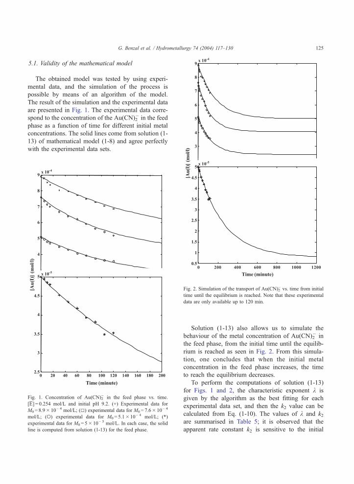
5.1. Validity of the mathematical model

The obtained model was tested by using experi-

mental data, and the simulation of the process is

possible by means of an algorithm of the model.

The result of the simulation and the experimental data

are presented in Fig. 1. The experimental data corre-

spond to the concentration of the Au(CN)2� in the feed

phase as a function of time for different initial metal

concentrations. The solid lines come from solution (1-

13) of mathematical model (1-8) and agree perfectly

with the experimental data sets.

G. Benzal et al. / Hydrom

Fig. 1. Concentration of Au(CN)2� in the feed phase vs. time.

[E] = 0.254 mol/L and initial pH 9.2. (+) Experimental data for

M0 = 8.9 10� 4 mol/L; (5) experimental data for M0 = 7.6 10� 4

mol/L; (o) experimental data for M0 = 5.110� 4 mol/L; (*)

experimental data for M0 = 5 10� 5 mol/L. In each case, the solid

line is computed from solution (1-13) for the feed phase.

Fig. 2. Simulation of the transport of Au(CN)2� vs. time from initial

time until the equilibrium is reached. Note that these experimental

data are only available up to 120 min.

Solution (1-13) also allows us to simulate the

behaviour of the metal concentration of Au(CN)2� in

the feed phase, from the initial time until the equilib-

rium is reached as seen in Fig. 2. From this simula-

tion, one concludes that when the initial metal

concentration in the feed phase increases, the time

to reach the equilibrium decreases.

To perform the computations of solution (1-13)

for Figs. 1 and 2, the characteristic exponent k is

given by the algorithm as the best fitting for each

experimental data set, and then the k2 value can be

calculated from Eq. (1-10). The values of k and k2are summarised in Table 5; it is observed that the

apparent rate constant k2 is sensitive to the initial

Table 5

Computed values of the characteristic parameters k and controlling

parameter (apparent rate constant) k2 for different initial metal

concentrations M0 and [E] = 0.254 mol/L

Initial concentration

of Au(I) M0 (mol/L)

Characteristic

exponent k(min� 1)

Controlling parameter

(apparent rate constant)

k2 (min� 1)

5 10� 5 M � 0.00376 0.000523

5.110� 4 M � 0.00750 0.00245

7.6 10� 4 M � 0.00847 0.00300

8.9 10� 4 M � 0.00563 0.00205

Fig. 4. Theoretical percentage of total metal transported, M%E,

and metal concentration when the equilibrium is reached,

Ml. [E ]=0.254 mol/L and initial pH 9.2. M0 = 5 10� 5

mol/L, Ml = 7.7 10� 6 mol/L, M%E = 84%; M0 = 110� 4

mol/L, Ml= 2.27 10� 5 mol/L, M%E = 77%; M0 = 2.5 10� 4

mol/L, Ml= 8.9 10� 5 mol/L, M%E = 64%; M0 = 5.110� 4

mol/L, Ml= 2.4 10� 4 mol/L, M%E = 52%; M0 = 7.6 10� 4

mol/L, Ml = 4 10� 4 mol/L, M%E = 46%; M0 = 8.9 10� 4

mol/L, Ml= 4.9 10� 4 mol/L, M%E = 43%.

G. Benzal et al. / Hydrometallurgy 74 (2004) 117–130126

metal concentration M0, and it is possible to establish

a relation between them as:

(4-2)k2 ¼ bðM0Þa

By plotting lnk2 vs. lnM0 (Fig. 3), a linear regression

allows us to compute the values of a = 0.65 and

lnb =� 1.06.

5.2. Estimation of the maximum percentage of

transported metal during the cotransport process

The concentration of Au(I) at the equilibrium,

Ml, given in Eq. (1-9) allows us to estimate theo-

retically the maximum percentage of transported

metal. These percentages are given by M%E=(M0�Ml/M0) 100 Eq. (1-12) and are represented in Fig.

4. In the same figure, it is observed that the percent-

Fig. 3. lnk2 vs. lnM0. (o) Values from Table 5. The straight line is

the plot of the linear regression lnk2 = alnM0 + lnb where a= 0.65and lnb=� 1.06.

age of transported metal increases when the initial

metal concentration decreases, and that the best

transport (84%) corresponds to M0 = 5 10� 5 mol/L.

A similar behaviour is observed for several initial

metal concentrations.

This indicates that the model is also sensitive to

the extractant concentration and suggests that a

possible way to increase the percentage of trans-

ported metal for a given initial metal concentration

is to increase the extractant concentration. This

sensitivity and behaviour is discussed in the next

section.

5.3. Sensitivity of the model to the extractant

concentration

It is important to note that model (1-8) is also

sensitive to the extractant concentration [E], as will be

shown in Figs. 5 and 6. This sensitivity can also be

explained in terms of the controlling parameter k2,

because [E] and k2 are related by Eq. (1-10).

Fig. 5 shows that the model agrees well with the

experimental data corresponding to the transport of

Au(I) for different extractant concentration [E]. From

Fig. 5. Concentration of Au(I) vs. time in feed phase.M0 = 5 10� 5

mol/L and initial pH 9.2. (5) Experimental data for [E] = 0.445 mol/

L (k2 = 0.44 10� 3 min� 1); (*) experimental data for [E] = 0.254

mol/L (k2 = 5.2 10� 4 min� 1). The solid line is the plot of solution

(1-13) in the feed phase.

G. Benzal et al. / Hydrometallurgy 74 (2004) 117–130 127

this figure, it is clear that the velocity of the process is

great for higher extractant concentration.

The percentage of metal transported represented in

Fig. 6 has been estimated theoretically by Eq. (1-12),

and it is observed that a 43% increase in extractant

concentration gives an increase of only 6% in the

Fig. 6. Theoretical extraction percentage of total metal transported,

M%E, when the equilibrium is reached. M0 = 5 10� 5 mol/L.

[E ] = 0.127 mol/L, M%E = 74%; [E] = 0.191 mol/L, M%E = 80%;

[E] = 0.254 mol/L, M%E = 84%; [E] = 0.382 mol/L, M%E = 88%;

[E] = 0.445 mol/L, M%E = 90%.

percentage of metal transported when the initial metal

concentration is M0 = 5 10� 5 mol/L.

5.4. Simulation of the behaviour of the pH in the feed

phase

The sensitivity of the proposed model to proton

concentration in the feed phase is explained in this

section, and the simulation of the behaviour of the pH

in the feed phase is carried out.

It is known that in the cotransport of the Au(I), the

protons are transported with the metal at the stripping

phase. Therefore, the proton concentration in the feed

phase decreases during the process as predicted by the

Eq. (1-6) as:

½Hþ� ¼ ½Xf ðtÞ� ¼Kw=n

½Y� � ½Mf �ðtÞ

From this equation, we can simulate the behaviour of

pH in the aqueous feed phase considering the equality

pH= � log[H+]. The behaviour of the pH for different

experimental data sets is seen in Fig. 7. From this

simulation, it is observed that when the initial metal

concentration increases, the pH at the steady state also

increases. Therefore, the protons concentration

decreases. This agrees with the mechanism of the

cotransport phenomenon and allows us to validate

model (1-6).

Fig. 7. Simulation of the behaviour of the pH vs. time in the feed

phase. [E] = 0.254 mol/L and initial pH 9.2. (—) M0 = 5 10� 5

mol/L; (– -– ) M0 = 7.6 10� 4 mol/L; (---) M0 = 110� 4 mol/L;

(—) M0 = 8.9 10� 4 mol/L.

etallurgy 74 (2004) 117–130

5.5. Simulation of the behaviour of metal complex

concentration in membrane phase and the metal

concentration in the stripping phase

For the simulation of the behaviour of the metal

complex concentration U (t) in the membrane phase,

G. Benzal et al. / Hydrom128

Fig. 8. (a) Evolution of the Au(I) concentration in the different

phases. M0 = 5 10� 5 mol/L, [E] = 0.254 mol/L, initial pH 9.2.

jkj= 0.003 min� 1, k2 = 5.2 10� 4 min� 1, Deff = 3.7 10� 7 dm2/

min; (1) *Experimental data for feed phase. The solid line is the plot

of solution (1-13) forMf vs. time. (2)U vs. time. The plot of solution

(2-11) for the membrane phase. (3)MS vs. time. The plot of solution

(3-3) for the stripping phase. (b) Evolution of the number of moles of

the Au(I) in the different phases. (a) nf(t) number of moles in the feed

phase. (b) 20nm(t) number of moles in the membrane phase. Twenty

is a scale factor for a better visualisation. (c) nS(t) number of moles in

the stripping phase. (d) Plot of the mass balance equation nf + nm+ nS.

solution (2-11) has been computed in the algorithm.

We notice that, due to the very small dimensions of

the membrane phase, it is not possible to obtain

experimental data on the metal complex concentra-

tion. Therefore, the simulation of metal complex

concentration and the number of moles of metal

complex in the membrane phase are analysed by the

behaviour expected for the metal complex as seen in

Fig. 8a and b, respectively. In Fig. 8a, the metal

concentrations in the three phases are simulated

simultaneously from the transient until equilibrium

is reached.

In Fig. 8b, the number of moles in each phase is

simulated simultaneously. As a final numerical check,

it can be seen that 1-13), (2-11) and (3-3) satisfy the

mass balance equation given by Eq. (3-6).

6. Conclusions

A mathematical model that describes the transport

of metal species a through flat sheet-supported liquid

membrane (FSSLM) is derived.

The advantages of the model are that it:

– consists of approximate equations for each phase,

given by Eqs. (1-13), (2-11) and (3-3), which

describe the concentration variations in the tran-

sient in terms of initial conditions and the in-

dependently measurable parameters;

– takes into account the chemical reaction in the

interface, the driving force between the feed and

stripping phase and the diffusion in the membrane

phase;

– is sensitive to the variation of initial metal

concentration and extractant concentration;

– allows us to reproduce the evolution of the

metal (concentration and number of moles) in

the feed and stripping phase and to simulate

the behaviour of the metal complex in the

membrane;

– relies on a nonconstant concentration of the species

whose gradient is the driving force and permits one

to simulate the evolution of the pH in the feed

phase in the transient as a function of metal

concentration;

– permits us to compute theoretically the maximum

percentage of metal transported;

G. Benzal et al. / Hydrometallurgy 74 (2004) 117–130 129

– allows us to estimate the value of the rate constant,

which is the controlling parameter of the velocity

of the process;

– is analytically solved and numerically implemented;

– reproduces with high accuracy the transport of

metal ion in alkaline solution when checked

against experimental data corresponding to the

transport of Au(CN)2� in alkaline solution by

LIX 79.

Nomenclature

Aeff effective interfacial area (dm2)

bi(t) generalised Fourier coefficients.

C metal ion in membrane and stripping phase

[C] metal ion concentration in membrane and

stripping phase (mol/L)

d membrane diameter (dm)

Deff effective membrane diffusion coefficient of

the metal in organic phase (dm2/min)

DE diffusion coefficient of the extractant in the

membrane phase (dm2/min)

E extractant (carrier) in membrane phase

[E] extractant concentration (mol/L)

kf forward rate constant ((dm2)2 min� 1 mol� 2)

kr reverse rate constant (min� 1)

k1 apparent forward rate constant (1/mol2 min)

k2 apparent reverse rate constant (controlling

parameter). (min� 1)

Kex extraction constant at feed–membrane

interface

Kw ionic product of water

K proportionality constant

L membrane thickness (cm)

Mf metal species in feed phase

M0 initial metal concentration in feed phase

(mol/L)

M%E metal extraction percentage

Ml equilibrium point [metal concentration in

aqueous feed phase in the steady state

(mol/L)]

[Mf] metal concentration in feed phase as a

function of time (mol/L)

[MS] metal concentration in stripping phase as a

function of time (mol/L)

MlS equilibrium point [value of metal concentra-

tion in stripping phase in the steady state

(mol/L)]

m, n the charge of ions

n0 initial number of moles in the feed phase

nlf number of moles in the feed phase in the

steady state

nf(t) number of moles in the feed phase at time t

nm(0,t) number of moles in the first interface at

time t

nm(L,t) number of moles in the second interface at

time t

nm(t) number of moles in the membrane phase at

time t

nS(t) number of moles in the stripping phase at

time t

R stripping reagent (mol/L)

[R] concentration stripping phase reagent

(mol/L)

t time variable (min)

u(x,t) metal complex concentration in membrane

phase as a function of time and the thickness

of the membrane (mol/L)

u(0,t) metal complex concentration at feed–mem-

brane interface (mol/L)

u(L,t) metal complex concentration at membrane-

stripping interface (mol/L)

U (t) average concentration of the complex in the

membrane phase (mol/L)

V0 organic volume (dm3)

Vwf aqueous volume in the feed phase (dm3)

VwS aqueous volume in the stripping phase

(dm3)

Xf species whose gradient concentration be-

tween the feed and stripping phase is the

driving force of the process

[Xf] concentration of the specie Xf (mol/L)

x thickness variable (dm)

Greek letters

e porosity of the SLM

s tortuosity of the membrane

a linear coefficient in the linear regression

b independent coefficient in the linear

regression

k eigenvalue obtained from the stability study

(min� 1)

ki eigenvalues obtained from separation of

variables and Fourier series

ui(x,ki) eigenfunctions corresponding to kiR real field

p pi number

G. Benzal et al. / Hydrometallurgy 74 (2004) 117–130130

Subscripts

f and s feed and stripping solutions respectively

w aqueous phase

o organic phase or initial condition

l infinity time or steady state

Acknowledgements

This work was supported by the MCYT (PPQ2002-

04267-C03-03) and DURSI SGR2001-00249. G.

Benzal gratefully acknowledges economic support

from F.O.M.E.C. in the form of a fellowship grant at

the Universidad Nacional de Tucuman, Tucuman,

Argentina.

References

Baker, R.W., Tutle, M.E., Kelly, D.J., Lonsdale, H.K., 1977. Cou-

ple transport membranes: I. Copper separations. J. Membr. Sci.

2, Dover Publications, New York, p. 213.

Bear, J., 1972. Dynamics of Fluid in Porous Media. Dover

Publications, New York.

Bird, R.B., Stewart, W.E., Lightfoot, E.N., 1992. Fenomenos

de Transporte. Reverte Editorial Reverte S.A., Barcelona,

Espana.

Chrisstoffels, L.A.J., de Jong, F., Reinhoudt, D., 1996. ACS Ser,

vol. 642. American Chemical Society, Washington, DC, p. 18.

Chap. 3.

Crank, J., 1975. The Mathematics of Diffusion. Oxford University

Press Inc., New York.

Cussler, E.L., 1971.Membranes which pump. AIChE J. 17 (6), 1300.

Cussler, E.L., 1997. Diffusion. Mass Transfer in Fluid Systems.

Cambridge Univ. Press, United States of America.

Daiminger, U.A., Geist, A.G., Nitsch, W., Plucinski, P.K., 1996.

Efficiency of hollow fiber modules for non dispersive chemical

extraction. Ind. Eng. Chem. Res. 35, 184.

Danesi, P.R., 1992. Solvent extraction kinetics. In: Rydberg, J.,

Musikas, C., Chopin, G.R. (Eds.), Principles and Practice of

Solvent Extraction. Marcel Dekker, New York, pp. 157–207.

Danesi, P.R., Horwitz, E.P., Vandegrift, G.F., Chiarizia, R., 1981.

Mass transfer rate through liquid membrane: interfacial chemi-

cal reactions and diffusion as simultaneous permeability control-

ling factors. Sep. Sci. Technol. 16 (2), 201.

Gyves, J.D., Rodrigues de San Miguel, E., 1999. Metal ion sepa-

rations by supported liquid membranes. Ind. Eng. Chem. Res.

38 (6), 2182–2202.

Haberman, R., 1998. Elementary Applied Partial Differential Equa-

tions, 3rd Edition. Prentice-Hall.

Hirsch, M.W., Smale, S., 1983. Differential Equations, Dynamical

Systems, and Linear Algebra. Alianza Editorial, Madrid.

Ho, W.S.W., Sirkar, K.K., 1992. Membrane Handbook Van Nos-

trand-Reinhold, New York.

Huang, T.-C., Juang, R.-S., 1988. Rate and mechanism of divalent

metal transport through supported liquid membrane containing

di(2-ethylhexyl) phosphoric acid as a mobile carrier. J. Chem.

Technol. Biotechnol. 42, 3–17.

Ibanez, J.A., Victoria, L., Hernandez, A., 1989. Flux and charac-

teristic parameters in mediated transport through liquid mem-

branes. A theoretical model. Sep. Sci. Technol. 24 (1,2), 157.

Komasawa, I., Otake, T., Yamashita, T., 1983. Mechanism and

kinetics of copper permeation through a supported liquid mem-

brane containing a hydroxyoxime as a mobile carrier. Ind. Eng.

Chem. Fundam. 22, 127.

Madi, A., 1998. Doctoral Thesis, Universitat Politecnica de Cata-

lunya, Spain.

MATLAB, 1984–2000. The language of technical computing. Ver-

sion 6.0. Release 12. Copyright 1984–2000. The Math works.

Misra, B.M., Gill, J.S., 1996. ACS Ser, vol. 642. American Chem-

ical Society, Washington, DC, p. 361. Chap. 25.

Palis Jr., J., de Melo, W. 1998. Geometric Theory of Dynamical

Systems. Springer-Verlag, New York.

Plucinski, P., Nitsch, W., 1988. The calculation of permeation rates

through supported liquid membranes based on the kinetics of

liquid– liquid extraction. J. Membr. Sci. 39, 43.

Randall, T.P., John, L., 1996. ACS Ser, vol. 642. American Chem-

ical Society, Washington, DC, p. 57. Chap. 4.

Zachmanoglou, T., 1986. Introduction to Partial Differential Equa-

tions with Applications. Dover Publications, New York.